Landscape Models and Explanation in Landscape Ecology—A Space for Generative Landscape Science?

Daniel G. BrownUniversity of Michigan

Richard AspinallMacaulay Institute

David A. BennettUniversity of Iowa

Further development of process-based spatial models is needed to facilitate explanation in landscape ecology. Wediscuss the dual modeling goals of prediction and explanation and identify challenges faced in explaining land-scape patterns. These challenges are especially acute in attempts to explain patterns that result from complexadaptive systems. We compare examples of two process models used to describe landscape changes in YellowstoneNational Park as a consequence of predator-prey interactions. Generative landscape science is offered as acomplementary approach to explanation, combining models of candidate processes that are believed to give rise toobserved patterns with empirical observations. Key Words: complex systems, spatial modeling, spatial pattern.

Acentral theoretical concern in landscapeecology is understanding the interaction

between observed landscape patterns and a di-verse set of social and environmental processes.The domain of landscape ecology in the UnitedStates has been defined, primarily, around thecauses and consequences of spatial pattern, ex-pressed primarily in terms of biotic and abioticprocesses (Naveh 1982; Risser, Karr, and For-man 1984; Turner 1989; Nassauer 1995; Mlad-enoff and Baker 1999; Turner, Gardner, andO’Neill 2001). Although Turner, Gardner, andO’Neill (2001, 7) ‘‘do not think it necessary toinclude a human component explicitly in thedefinition of landscape ecology,’’ we take a moreinclusive view, derived from the European or-igins of landscape ecology (Naveh 1982), thatconcerns itself not just with the interaction oflandscape pattern with biophysical processes,but also with human actions. This view wouldseem essential to any attempts to make claimsabout the implications and/or appropriatenessof management interventions, and to contributeto the emerging ‘‘integrated land science’’ de-scribed by Klepeis and Turner (2001). Models oflandscape change have been used extensively to

study the effects of both natural and humanprocesses on landscape patterns since the emer-gence of landscape ecology in the United Statesduring the 1980s (Baker 1989).

An important thread of work in geographicinformation science (GIScience) deals with spa-tial models that can formally represent patternsand processes (e.g., Goodchild, Parks, andSteyaert 1993). Pattern-based models focus ondescribing spatial distributions and identifyingcorrelates of those distributions (e.g., Guisanand Zimmermann 2000), whereas process-based models describe process using a numberof different representations of mechanisms.Among the variety of purposes for which land-scape models are built, two are most importantin driving the nature and structure of models: (1)to make inferences about how and why land-scapes change, sometimes (not always) with theintent to produce more favorable outcomes, and(2) to predict future landscape states and pat-terns. These two goals are difficult to separatefrom one another. On the one hand, we canhardly expect to make reasonable predictionsabout future landscape patterns if we do nothave reasonable explanations for how they

The Professional Geographer, 58(4) 2006, pages 369–382 r Copyright 2006 by Association of American Geographers.Initial submission, March 2005; revised submissions, January 2006; final acceptance, April 2006.

Published by Blackwell Publishing, 350 Main Street, Malden, MA 02148, and 9600 Garsington Road, Oxford OX4 2DQ, U.K.

change. On the other hand, given a particularexplanation, encoded in a model, we commonlyuse the model’s predictive ability as the funda-mental measure of its veracity.

Assuming that science as science is built on gen-eral explanations, we focus in this article on theuse of process models in landscape ecology forbuilding explanations of landscape patterns anddynamics. Parunak, Savit, and Riolo (1998)made a useful distinction between two forms ofprocess models, both of which encode mecha-nisms: equation-based models and agent-basedmodels (ABMs). In GIScience, equation-basedmodels might be understood as a special class ofmodels that describe the processes by which at-tributes change at locations, which we refer tohere as location-based models. We provide exam-ples of an equation-based model and an ABMfrom research on landscape change in Yellow-stone National Park.

We hope to illustrate how the use of modelsfor explanation in landscape science representsan important frontier. We believe there is anopening for further integration of GIScienceand landscape ecology in the development of anapproach to the science that we, borrowingfrom but also going beyond Epstein and Axtell(1996) and Epstein (1999), refer to as ‘‘gener-ative landscape science.’’ Generative scienceconcerns itself with understanding how micro-level processes can generate macrophenomena(Epstein 1999). For a generative landscape sci-ence, the outcome or phenomenon of interest istypically spatial pattern, though some elementsof the dynamics may be of interest, for example,a sudden surge of landscape change that lagssome environmental or social change. Workis well underway in a number of quarters todevelop the theory and tools required for thisscience in both landscape and urban studies(Manson 2001; D. C. Parker et al. 2003; Ben-enson and Torrens 2004; Laney 2004; Brownet al. 2005). Here we hope to identify how spa-tial modeling tools in GIScience contribute to agenerative landscape science and how that sci-ence can contribute in the context of the largelyempirical emphasis of much of landscapeecology (Malanson 1999).

The Challenges of Explanation

An important characteristic of a scientific ex-planation (i.e., Popper 1959; Salmon 1984) is

that it describes the process (the why or how) bywhich a phenomenon happens. In other words,it contains falsifiable cause and effect state-ments. Explanations are clearly distinct fromempirical observations that describe patterns ofa phenomenon, including its characteristics(what) and the locations (where) or times (when)it occurs. Models of process and observations ofpattern, therefore, have complementary roles inlandscape ecology. Though process models areimportant tools with which we can encode ex-planations, we contend that many of the modelsin landscape ecology and, especially, land coverchange, are models of pattern, rather than ofprocess. In pointing the way forward, we focusour discussion on models of process.

Some explanations are necessarily limited toparticular places, others are generalizable con-cepts or processes that apply to a set of, or all,places. In the context of landscape change,processes and the relative importance of proc-esses are variable from place to place, dependingon the characteristics of the natural and humansystems that exist at these locations. This issuebrings to mind the discussions about the idio-graphic versus nomothetic nature of geography(Schaefer 1953). The nearest geography has to ageneral law, Tobler’s first law of geography (Sui2004), refers to pattern rather than process. It isa description of the general organization ofspace (i.e., near things are more related thandistant things), rather than a statement abouthow or why space is organized in the way that itis. As a ‘‘law’’ it is intended to refer to all placesrather than to a specific place.

We wish to highlight two important chal-lenges in increasing our understanding throughanalysis of interactions between patterns andprocesses. The first is a well-known problem inspatial analysis that we refer to here as the in-ference problem (Figure 1A), which is that a givenpattern (described through a finite number ofdimensional metrics) can result from multipleprocesses (Fotheringham and Brunsdon 2004).For example, if we observe a fragmented patternof forest (e.g., measured using statistics describ-ing patch numbers and sizes), there is no a prioribasis, without additional information, for con-cluding that the forest is fragmented because ofthe spatial pattern of logging or other distur-bance activity or because it is growing in an areaof patchy soil resources. Models that generateforest patterns through these two processes

370 Volume 58, Number 4, November 2006

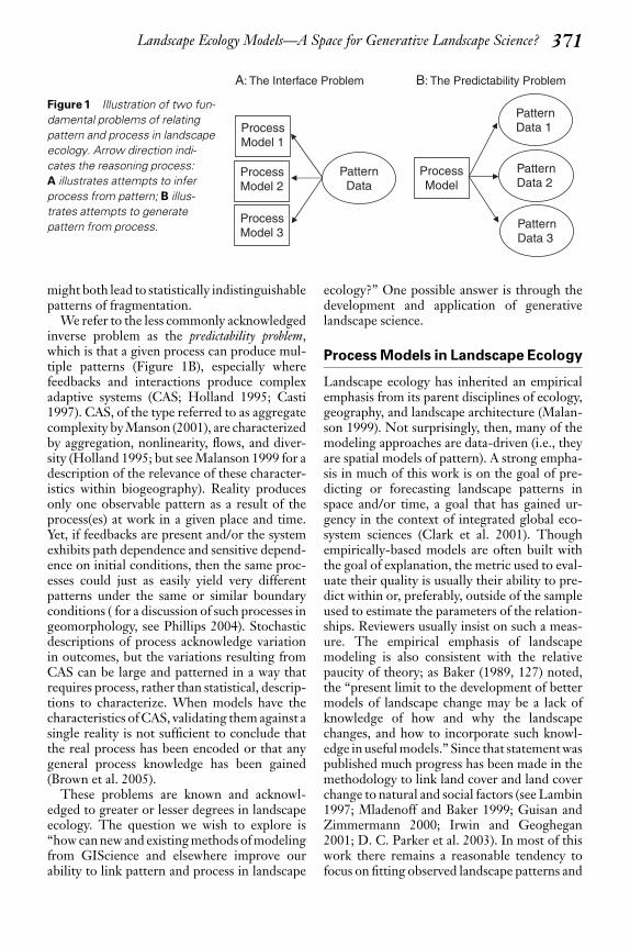
might both lead to statistically indistinguishablepatterns of fragmentation.

We refer to the less commonly acknowledgedinverse problem as the predictability problem,which is that a given process can produce mul-tiple patterns (Figure 1B), especially wherefeedbacks and interactions produce complexadaptive systems (CAS; Holland 1995; Casti1997). CAS, of the type referred to as aggregatecomplexity by Manson (2001), are characterizedby aggregation, nonlinearity, flows, and diver-sity (Holland 1995; but see Malanson 1999 for adescription of the relevance of these character-istics within biogeography). Reality producesonly one observable pattern as a result of theprocess(es) at work in a given place and time.Yet, if feedbacks are present and/or the systemexhibits path dependence and sensitive depend-ence on initial conditions, then the same proc-esses could just as easily yield very differentpatterns under the same or similar boundaryconditions ( for a discussion of such processes ingeomorphology, see Phillips 2004). Stochasticdescriptions of process acknowledge variationin outcomes, but the variations resulting fromCAS can be large and patterned in a way thatrequires process, rather than statistical, descrip-tions to characterize. When models have thecharacteristics of CAS, validating them against asingle reality is not sufficient to conclude thatthe real process has been encoded or that anygeneral process knowledge has been gained(Brown et al. 2005).

These problems are known and acknowl-edged to greater or lesser degrees in landscapeecology. The question we wish to explore is‘‘how can new and existing methods of modelingfrom GIScience and elsewhere improve ourability to link pattern and process in landscape

ecology?’’ One possible answer is through thedevelopment and application of generativelandscape science.

Process Models in Landscape Ecology

Landscape ecology has inherited an empiricalemphasis from its parent disciplines of ecology,geography, and landscape architecture (Malan-son 1999). Not surprisingly, then, many of themodeling approaches are data-driven (i.e., theyare spatial models of pattern). A strong empha-sis in much of this work is on the goal of pre-dicting or forecasting landscape patterns inspace and/or time, a goal that has gained ur-gency in the context of integrated global eco-system sciences (Clark et al. 2001). Thoughempirically-based models are often built withthe goal of explanation, the metric used to eval-uate their quality is usually their ability to pre-dict within or, preferably, outside of the sampleused to estimate the parameters of the relation-ships. Reviewers usually insist on such a meas-ure. The empirical emphasis of landscapemodeling is also consistent with the relativepaucity of theory; as Baker (1989, 127) noted,the ‘‘present limit to the development of bettermodels of landscape change may be a lack ofknowledge of how and why the landscapechanges, and how to incorporate such knowl-edge in useful models.’’ Since that statement waspublished much progress has been made in themethodology to link land cover and land coverchange to natural and social factors (see Lambin1997; Mladenoff and Baker 1999; Guisan andZimmermann 2000; Irwin and Geoghegan2001; D. C. Parker et al. 2003). In most of thiswork there remains a reasonable tendency tofocus on fitting observed landscape patterns and

A: The Interface Problem B: The Predictability Problem

Process Model 1

Process Model 2

Process Model 3

Pattern Data

Process Model

Pattern Data 1

Pattern Data 2

Pattern Data 3

Figure 1 Illustration of two fun-

damental problems of relating

pattern and process in landscape

ecology. Arrow direction indi-

cates the reasoning process:

A illustrates attempts to infer

process from pattern; B illus-

trates attempts to generate

pattern from process.

Landscape Ecology Models—A Space for Generative Landscape Science? 371

on predictive accuracy as the primary measuresof a model’s veracity (Pontius 2002; Pontius,Shusas, and McEachern 2004). But to build ourunderstanding of landscape systems, and ex-plain the human and environmental drivers ofchange in those systems, landscape ecology canmake better use of the power of additional ap-proaches to spatial-process-based modelingthat are being developed within GIScience.

What Dobson (1992) referred to as processlogic, and contrasted with spatial logic, proceedsfrom our understanding, intuition, formalproofs, or guesses of how the world works todeductions about specific outcomes (i.e., pat-terns) that can be observed and tested in theworld. Popper (1959) describes scientific inves-tigation, in practice, as an alternating process ofdeduction (loosely related to process logic) andinduction (in the case of geography, spatial log-ic). Computer simulation models of processwithin GIScience provide tools to bolster theiterative nature of this cycle in landscape ecol-ogy. Simulations have a longer history in phys-ical geography than in human geography,though new tools are making it possible thereas well (e.g., D. C. Parker et al. 2003; Benensonand Torrens 2004). The processes derived fromour understanding are necessarily general innature, though the relative importance of var-ious factors or parameters can be adjusted (i.e.,calibrated) to fit specific cases.

Scale is, of course, a matter of serious concernfor geographers. One important scale issue in-volves the level of generality of that which wewish to explain or predict. In some instances,our goal relates to predicting specific outcomesat specific times and locations (e.g., will devel-opment happen in this place or another in tenyears?). We would argue that because such pre-dictions are specific, they are less suited to ex-planation in the general sense, and hence tryingto achieve the goal of predicting finely grainedpatterns can conflict with the goal of generalexplanation. In a science of landscapes, scien-tific explanation should presumably occur at thelevel of the landscape (i.e., the macrophenome-non)—explaining why cities have particular pat-terns (e.g., sprawl), why landscapes get more/less fragmented over time, or why ecotones areabrupt or gradual. This approach mirrors ‘‘pat-tern-based modeling,’’ described recently byGrimm et al. (2005). These macrophenomenarepresent empirically observable structures that

might or might not have general or commoncauses. Spatiotemporal pattern characteristics,like those measured with landscape patternmetrics (LPMs) or temporal trajectories, canserve as indicators of such macrophenomena(D. Parker and Meretsky 2004). For example,Malanson and colleagues have used spatialmodels to identify how patterns at the alpinetreeline ecotone might have formed as a result ofenvironmental feedbacks (Bekker et al. 2001;Malanson 2001; Malanson, Xiao, and Alftine2001; Alftine and Malanson 2004; Malanson,Zeng, and Walsh 2006).

A second scale issue relates to the spatial scaleof representation, in this case representation ofprocess. If we are to represent geographicallandscape processes well, we need to be able torepresent them at the scales at which theseprocesses operate. Cause and effect representa-tions that are applied to spatially aggregate phe-nomena clearly pose challenges for actuallyrepresenting the mechanisms (the how or why)that cause many observed landscape relation-ships, as our understanding of the ecological fal-lacy cautions in statistical analysis (Robinson1950). However, neither is it sufficient to alwaysseek the finest level of disaggregation possible,because processes operate across scales and can,therefore, result in informative empirical rela-tionships at multiple scales (Walsh et al. 1999).Similar issues of scale are of concern in our rep-resentations in the temporal dimension; that is,temporal patterns and cycles can be observedover varying time scales, and time intervals ofobservation need to sufficiently resolved toobserve processes of various rates.

Location-Based Models

A whole generation of landscape simulationmodels has used locations on the landscape astheir most fundamental representational unit,and usually represent the change process as adiscrete event in which the landscape typechanges at that location. These models oftentake the form of cellular models of discreteevents of change, such as cellular automata, or oftransition probabilities (e.g., Turner 1987; Bak-er 1989; Berry et al. 1996; Batty, Couclelis, andEichen 1997; Lambin 1997; White and Engelen1997; Clarke and Gaydos 1998; Brown et al.2002). Such models can incorporate dynamicsand feedbacks and, therefore, can representCAS (Theobald and Hobbs 1998). However,

372 Volume 58, Number 4, November 2006

their utility for explanation can be limited bytheir sometimes nonintuitive relationship be-tween the process as expressed in the model (i.e.,through spatial factors that affect transitions ortransition probabilities) and our intuition aboutlandscape change (i.e., that it is carried out byorganisms and actors that take actions andchange landscapes). Landscapes do not changespontaneously; they are changed by the action of or-ganisms, human agents, and natural disturbanceprocesses.

Representing transitions as heuristic or pro-babilistic events can limit our ability to explainthe mechanisms. For example, a statement ofthe form ‘‘forest clearing is more likely at loca-tions that have better soil’’ may be consistentwith observations, and the patterns simulatedbased on it may match observed patterns well,but why this relationship exists remains open tointerpretation. Is it because these sites grow thetypes of trees that are in demand on the timbermarket, or because these sites are most desiredfor clearing, settlement, and agriculture? Howcan we adjudicate among alternative explana-tions? Of course, which process is ultimately thecorrect one has implications for implementingpolicies or management plans intended toachieve a particular landscape pattern.

One way to improve the level of explanationencoded in transition-based models is to useanalytical equations that actually describe howthe changes are made. So-called equation-basedmodeling is a specific case of location-basedmodeling that uses mathematical descriptionsof processes, as opposed to fitted heuristic orstochastic representations. The following is asimplified example that illustrates how equa-tion-based models of predator-prey processescan be represented spatially to describe vegeta-tion change in Yellowstone National Park.

Example of an Equation-Based Model

In the wintertime, elk movements within Yel-lowstone National Park can be modeled as abalance between two competing objectives:maximizing net bioenergetic return and mini-mizing the risk of predation. Vegetation bio-mass on the landscape serves as forage for elkand is affected by foraging pressure, plantphenology, and snow conditions. The proba-bility of elk death due to starvation is a functionof this biomass and an elk’s ability to efficientlyfind and consume forage. Likewise, the spatial

pattern of elk presents a resource to wolves. Elkprefer areas with high levels of forage andwolves prefer areas with high elk numbers. Thelandscape can, therefore, be conceptualized astwo dynamic and interconnected potential sur-faces: one pulling elk and wolves toward loca-tions with high resource content, the otherpushing elk away from locations that possessdeep snow (rendering forage inaccessible) orhigh predation rates. The interconnectedness ofthese species, and the resulting spatial pattern ofresources and risks, creates feedback processesthat turn the landscape into a complex adaptivesystem (Figure 2).

The ideal free distribution (IFD) was pro-posed by Fretwell and Lucas (1970) to describethe optimal distribution of mobile consumers inrelation to their food resources, and it was usedto model landscape change within YellowstoneNational Park as a function of these interac-tions. Farnsworth and Beecham (1997) haveshown that the IFD is a limiting case of a moregeneral model developed from diffusion rela-tions; they give the general model as

vi

vj¼ pi

pj

� � 2b1þ2db�a�2gð Þ

; ð1Þ

where vi is the predator density in patch i, pi

is the prey density in patch i, a is a measureof departure from the IFD, b is a sensitivityparameter for the predator-prey relationship,d is a measure of reward rate, and g is a measureof decline in reward rate due to social aggrega-tion (or predation).

Both the IFD and the generalized Farnsworthand Beacham model (the IFD models) assumethat (1) habitat quality is distributed in homo-

Spatial pattern of forage

Spatialpattern of elk

Spatial pattern of wolves

Figure 2 The spatiotemporal dynamics of forage,

prey, and predator produces a complex adaptive

system.

Landscape Ecology Models—A Space for Generative Landscape Science? 373

geneous patches, (2) mobile organisms are om-niscient and can switch between patches withnegligible cost and in negligible time, (3) ani-mals switch patches to maximize their fitness,and (4) fitness is positively related to habitatquality and negatively related to the density ofothers in a patch. The formulation and assump-tions of these IFD models parallel the descrip-tion and representation of environmentalvariability using object (vector) data types.Patches are represented in a spatial database aspolygons, measures of habitat quality are rep-resented as attributes of polygons, and the IFDmodels evaluate the relative pairwise merits ofpatches to allocate predators in the landscape.This representation, although matching thenotation of the IFD models and the patch re-presentation commonly used by landscapeecologists and found in vegetation maps, rep-resents a static landscape pattern, even if thequality of patches varies between time steps,because the location and boundaries of patchestypically cannot change through time in eitherthe GIS or IFD models. The area betweenpatches, the matrix, plays no part in the evalu-ation of patches. In essence, the IFD modelsimplemented using a patch/polygon representa-tion of environmental variability are a nonspatialtype of model, albeit one that can produce aspatial representation of the relative quality ofpatches as a measure of fitness for predators.

An alternative implementation of this modelcan be developed using a field- (raster-) basedrepresentation of environmental variability(Lees 1996). This representation treats individ-ual grid cells as the objects of interest. An ad-ditional modification to the model is to treat thevarious parameters of the model as functions ofthe local geographical neighborhood for eachgrid cell. Thus the reward rate (d) and decline inreward rate due to social aggregation or preda-tion (g) are expressed as functions of the sum ofthe prey/habitat quality within distance w ofeach grid cell. Distance w can vary for d and g.For the example of elk and wolves, these dis-tances may vary based on habitat type and thebehavioral ecology of the species. Logistic func-tions for d and g are used in this example. Thesefunctions for d and g represent the spatial be-havior of individual animals in relation to theirresources and in response to their own and otherspecies. The form of the functions can be con-structed from field experiments or empirical

studies of animal spacing and resource use. Thispresents an opportunity for field landscapeecology to provide inputs on animal behaviorto theory-based models, in this case a geograph-ically-modified IFD model.

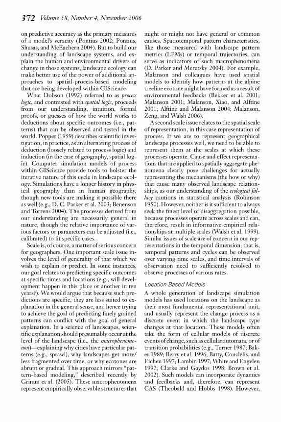
Solving the model (Equation [1]) for each pi-xel produces estimates for the distribution of elkand wolves at a particular time step (Figures 3Aand 3B). The elk model is then used to updatethe biomass dataset and the models are againcomputed for the next time step (Figure 3C).Interactions between wolves and elk are thusexplicitly represented in the model steps and canalso be mapped at each time step or as a movie.

This approach has a number of advantages.First, the result is a temporally and spatially dy-namic model of the interaction of environmen-tal conditions, plant biomass, and elk andwolves, giving insight into the spatial and tem-poral dynamics of the system. Second, by using araster representation of environmental hetero-geneity, the model can be linked with other data,such as snow depth, that modifies the environ-ment of the study area by relating the time stepof the model to calendar time. Third, a variety ofmacrolevel outcomes can also be evaluated;these are of interest in their own right and mayalso help to validate the model (Bart 1995). Forexample, model outputs of interest might in-clude density of animals integrated over time forspecific patches, population distributions in dif-ferent parts of the study area at different times,or potential impacts on vegetation based onmodeled densities of elk in different parts of thestudy area summed over the winter. Finally, themodel outputs can be evaluated with all avail-able field data since they have not used any fielddata in their development; this avoids the con-founding of training and validation datasets thatcan pose problems for pattern-based models.

Agent-Based Models

The recent development of individual-basedmodels (IBMs) and ABMs (DeAngelis andGross 1992; D. C. Parker et al. 2003) repre-sents an opportunity to improve on the processrepresentations enabled by equation-basedmodels of locations. Individuals or agents caninclude organisms, people, households, collec-tives, institutions, and the like. By representingthe behavior of each individual or agent, thesemodels can characterize the separateeffects of each at the appropriate scales and

374 Volume 58, Number 4, November 2006

simultaneously represent the interactions be-tween them, for the behavior of one agent in amodel affects the state or behavior of another.IBMs for generating landscape patterns, for ex-ample, track the growth of individual trees ordistributions of trees (He, Mladenoff, and Crow1999; Prentice and Leemans 1990) and the re-sponse of mobile organisms, including elk (Bian2003), to the environment (Westervelt andHopkins 1999). ABMs include models of farm-ers making decisions about crop types and man-agement techniques (Berger 2001; and Polhill,Gotts, and Law 2001; Balmann et al. 2002),

landowners making resource-allocation deci-sions (Evans et al. 2001), and home buyers mak-ing residential-location decisions (Benenson2004; Brown et al. 2005). The following exam-ple illustrates the use of agent-based modelingto represent the same predator-prey interac-tions in the Yellowstone ecosystem.

Example of an Agent-Based Model

Although location-based models, like the IFD-based model described above, necessarily makeassumptions concerning, for example, elk andwolf omniscience and their ability to compute

Figure 3 Distributions, after ten

time steps in the ideal free distri-

bution model, of (A) wolf density,

(B) elk density, and (C) biomass

for the Northern Range of

Yellowstone Park.

Landscape Ecology Models—A Space for Generative Landscape Science? 375

optimal strategies, these assumptions may limitthe ability of the model to accurately reflect theprocesses by which elk and wolves learn aboutand adapt to a continually changing environ-ment. Evolution may lead to near-optimal be-havior at the aggregate level, but it does notproduce individual elk with the cognitive abilityto deduce optimal routes. Instead, elk act onbounded situational and spatial knowledge anduncertain information to navigate throughcomplex landscapes during winter migration(Boyce 1989). Situational knowledge is alearned response to a perceived stimulus. Re-search suggests, for example, that an elk’s mi-gratory decisions (actions) are largely driven bysnow depth (K. L. Parker, Robbins, and Hanley1984; Sweeney and Sweeney 1984; Boyce 1989;Turner et al. 1994), perceived risks and resourc-es (stimuli), and past experience (Boyce 1989;Ripple et al. 2001; Creel and Winnie 2005; For-tin et al. 2005). Agent-based modeling, there-fore, complements the explanations providedby equation-based techniques by providing amechanism by which individual-level behaviorscan be explored.

Situational and spatial knowledge was incor-porated into an ABM of elk/wolf interaction tosimulate the spatial behavior of elk during theirwinter migration on Yellowstone’s NorthernElk Winter Range (NEWR). In ongoing re-search, machine-learning algorithms, specifi-cally evolutionary- and reinforcement-learningalgorithms, are used by elk agents to learn whento begin migrating in response to snow depth andwhere to migrate in response to the spatial pat-tern of risks and resources. Situational knowl-edge is represented as action/stimulus coupletsstored in a decision matrix. When-to-migrateknowledge, for example, is modeled as adecision matrix driven by the change in snowdepth from one time step to the next. Thevalues stored in the elements of this matrixrecord the probability of a migratory movement(the action) given a perceived change insnow depth (the stimulus). The learning algo-rithm attempts to maximize end-of-winter elkbody mass.

Spatial knowledge builds as elk repeatedlyinteract with the environment and learn how torespond to the spatial distribution of positive(e.g., high availability forage) and negative (e.g.,high predation risk) stimuli. This stored knowl-edge leads to more efficient and less risky

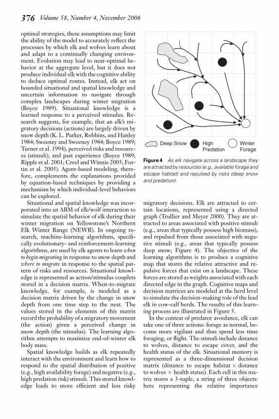
migratory decisions. Elk are attracted to cer-tain locations, represented using a directedgraph (Trullier and Meyer 2000). They are at-tracted to areas associated with positive stimuli(e.g., areas that typically possess high biomass),and repulsed from those associated with nega-tive stimuli (e.g., areas that typically possessdeep snow; Figure 4). The objective of thelearning algorithms is to produce a cognitivemap that stores the relative attractive and re-pulsive forces that exist on a landscape. Theseforces are stored as weights associated with eachdirected edge in the graph. Cognitive maps anddecision matrices are modeled at the herd levelto simulate the decision-making role of the leadelk in cow-calf herds. The results of this learn-ing process are illustrated in Figure 5.

In the context of predator avoidance, elk cantake one of three actions: forage as normal, be-come more vigilant and thus spend less timeforaging, or flight. The stimuli include distanceto wolves, distance to escape cover, and thehealth status of the elk. Situational memory isrepresented as a three-dimensional decisionmatrix (distance to escape habitat � distanceto wolves � health status). Each cell in this ma-trix stores a 3-tuple, a string of three objects:here representing the relative importance

Deep Snow High Predation

Winter Forage

Figure 4 As elk navigate across a landscape they

are attracted by resources (e.g., available forage and

escape habitat) and repulsed by risks (deep snow

and predation).

376 Volume 58, Number 4, November 2006

placed on foraging, maintaining vigilance, andflight given a specific combination of stimuli.Knowledge of the spatial pattern of risk islearned in a manner similar to the process de-scribed above. However, because wolves adaptto the changing spatial patterns of their prey, elkmust also learn to ignore or forget old knowl-edge that is no longer supported by more recentobservations.

ABMs like this one provide a means to explore(1) processes that drive individual-level behav-ior and interaction; (2) plausible hypothesesabout how aggregate-level patterns emergefrom individual-level behavior; (3) the impactthat heterogeneity and random disturbancehave on system outcomes; and (4) the conse-quences, expected and unexpected, of manage-ment decisions that are applied to CAS. Thesemodels are often inspired by, and thereforecomplement, the kinds of theories representedby equation-based simulations. However, manyof the same characteristics that make ABMsuseful also make them notoriously difficult tovalidate. It is not reasonable, for example, toexpect that the migratory path of an individual

virtual elk will match the path taken by a real elk.This difficulty of prediction creates a challengefor generative landscape science.

Challenge of Generative LandscapeScience

The goal of generative landscape science is ex-planation of landscape patterns—that is, to un-derstand the processes and conditions thatgenerate them (Grimm et al. 2005). The ap-proach is to use computer simulations that rep-resent the agents and behaviors that causechanges. Such methods, called bottom-up be-cause they work with an atomistic view of thesystem to derive system-level outcomes (i.e.,patterns), can have difficulty matching observedpatterns as well as statistically fitted models,such as aggregate and averaged patterns of elkmigration or household-level statistical rela-tionships (e.g., Laney 2004) and processes(D. C. Parker et al. 2003). In a simple empir-ical test of scaling properties, Laney (2004)found that aggregation of land cover patterns

Figure 5 A cognitive map produced by the learning algorithm illustrating the most likely routes taken by elk

to resource rich locations.

Landscape Ecology Models—A Space for Generative Landscape Science? 377

determined at the household level resulted in apoor match to observed patterns at larger scales.Jenerette and Wu (2001) developed a simulationto model land use change in central Arizona.Transition probabilities of the model were set intwo different ways: first, based on average ob-served transition rates for cells with varyingnumbers of urban neighbors; and second, basedon the outcome of a genetic algorithm that wastrained to fit observed spatial pattern, measuredthrough landscape pattern indices. Naturally,the model with optimized transition probabil-ities reproduced the landscape patterns sub-stantially better than the nonoptimized pattern.These two examples illustrate that it is hard tomatch landscape-level patterns by simply ag-gregating patterns and processes from a finerlevel of understanding.

Like the urge to ‘‘teach to the test’’ in edu-cation, there is a strong urge to focus on modelsthat maximize some measure that compares themodel output with real-world observations (i.e.,goodness of fit or prediction accuracy), some-times at the expense of intuition, deduction, andencoding of processes (Batty and Torrens 2001).The urge to fit model parameters to data has abasis in scientific rigor and is sensible when thegoal is prediction (or doing well on the test). Ithas led to novel methods to calibrate parametersand optimize fit to observed patterns throughback-casting (e.g., Clarke and Gaydos 1998;Jenerette and Wu 2001). However, when webuild models from the bottom up we need toacknowledge that we will not have all the datawe need and that the systems themselves maysimply be unpredictable. The insistence on pre-dictive power at the microlevel as the onlymeasure of the correctness of a model, there-fore, may be misplaced and has a number ofconsequences. First, although the goal is toproduce a reasonable representation of the proc-ess that produced the pattern, such fitting exer-cises focus instead on representation of thepattern itself. The logical problems associatedwith using goodness-of-fit measures to test theveracity of a model are described by Oreskes,Shrader-Frechette, and Belitz (1994), and in-clude the inference-laden nature of data and thefact that the systems they represent are neverclosed systems, as is implied by such compari-sons. Second, Brown et al. (2005) demonstrated,with a model of urban growth, how the urge tofit data in path-dependent systems can result in a

model that predicts the actual outcome too fre-quently (i.e., is overfit) because there is only oneobservation from the real process to compareagainst.

This leads us to an interesting issue: we mayunderstand well the processes that operate on alandscape, but still be unable to make accuratepredictions about the outcomes of those proc-esses. In these instances the processes them-selves are inherently unpredictable. Nonethe-less, refining our understanding—for example,about the predictability of the process—is stillan important and valuable activity.

The science of landscape ecology could ben-efit from greater integration of generative ap-proaches that complement both the inductiveand analytical-modeling approaches that aremore common in landscape science. The meth-ods, especially agent-based and individual-based modeling, are available. By encodingwhat we think we already know about process-es operating on a landscape, or about landscapeprocesses in general, and comparing the out-comes generated by those models with obser-vations, we can learn more about complexlandscape systems and identify avenues for fur-ther empirical or experimental investigation.Comparisons of insights derived from our em-pirical and inductive approaches with those de-rived from our deductive and process-basedapproaches holds particular promise.

We need new metrics for comparing modelsand empirical observations. There remains akey role for spatial analytical methods to defin-ing the outcomes in question, and comparingaggregate outcomes (e.g., D. Parker andMeretsky 2004). Brown et al. (2005) proposenew metrics for comparing model-producedpatterns with the one observed (or reference)pattern. The metrics acknowledge, first, that amodel can produce many (sometimes very dif-ferent) outcomes. Separate analysis of regionsthat are variant or invariant in model outcomescan help identify how well the model matches areference map (i.e., the one reality), as well ashow predictable the system appears to be, basedon the model. Grimm et al. (2005) argue thatcomparing many different patterns from themodel (e.g., spatial landscape patterns, tempo-ral trajectories, and health of a population) canprovide much stronger support for a model orexplanation. They suggest distinguishingbetween primary patterns—those that we seek

378 Volume 58, Number 4, November 2006

to explain—and secondary patterns—addition-al patterns in the world that our model outputcan be compared with for validation of itsmechanisms.

A generative component to landscape sciencecan help us to

� Develop and encode explanations thatcombine multiple scales. Because agentscan act on patterns at different scales(e.g., households on parcels, developerson subdivisions, and local governmentson jurisdictions), and because the out-come of interest is usually aggregate innature (e.g., overall pattern), generativelandscape science facilitates explanationsthat combine processes at multiple scales.

� Evaluate the implications of theory. Ep-stein (1999) refers to generative science asessentially ‘‘intuitionist’’; that is, it derivesits explanatory power from use of our in-tuition. Intuition is a reasonable startingplace for theory development and scien-tific investigation, but as system behaviorsget more and more complicated (e.g.,within CAS) it is difficult to intuit theoutcomes and, in many cases, our intuit-ions about the dynamics of CAS are mis-leading and biased by past experience,culture, and education. Understandingthe implications of our intuitions, andtraining them in the face of such com-plexity, can be helped with the use ofbottom-up models. One approach is toexplore the solution space of the model—for example, by ‘‘sweeping’’ the values ofthe parameters in the vein of sensitivityanalysis. Such analysis is akin to experi-ments in which we change the environ-ments or behaviors of actors in oursimulation model (i.e., experiments thatare impossible to do in the real world).For example, Schelling (1978) taught usthat agents with a surprisingly low level ofdesire for neighbors like themselves pro-duces a segregated settlement pattern.

� Identify and structure needs for empiricalinvestigation. The modeling advocatedhere is intended as a complement to, not areplacement for, empirical investigation.Data analysis and fieldwork are neededto identify patterns of interest and as asource of information about candidate

behaviors for individuals and agents. It isclear that empirical and experimentalwork is needed to evaluate the possiblemechanisms causing feedbacks, and theirrelative strengths. Models provide ameans to structure this empirical workwithin a conceptual framework and toevaluate the consequences of the findings.

� Deal with uncertainty. Though theGIScience and geostatistics literatureprovides much guidance on dealing withuncertainty in spatial data, Bankes (2002)identifies a kind of uncertainty—‘‘deepuncertainty’’— that is not well-character-ized by existing spatial modeling meth-ods. In addition to uncertainty (or error)in data and parameters, deep uncertaintyexists when there is uncertainty or disa-greement in the model or model struc-ture. Inadequate empirical support for, orthe necessary simplification of, the beha-vioral processes in a model are sources ofdeep uncertainty. By simulating processesat a level close to that of our understand-ing of behavior (e.g., at the agent orindividual level), we can substitutealternative assumptions or theories aboutbehavior and evaluate the aggregate out-comes of alternative model (e.g., rationaldecision-making versus bounded ration-ality versus satisficing).

At a minimum, incorporating ‘‘experiments’’based on models into our analysis of landscapepatterns can lead to the identification of inter-esting phenomena at the system level (e.g., tip-ping points, fragmentation or fractal patterns,and path dependence) using systems that aresimpler than, but representative of, the realworld. Also, we can hope to begin to recognizewhen prediction may not be a reasonable goal. Amore ambitious hope is that these models can beused to test, and even adjudicate between,multiple competing explanations, especiallythrough interaction and coordination withdata collection and experimentation.

Conclusions

We have outlined how the integration of spatialmodeling approaches from GIScience contrib-utes to our understanding of pattern-process

Landscape Ecology Models—A Space for Generative Landscape Science? 379

relationships in landscape ecology. In this sense,our arguments are aimed firmly at developingGIScience modeling in support of landscapeecology theory and explanation. In this sense,the representational tools of GIScience bringanalytical power to the science of landscapeecology. The two examples we provide of rep-resenting elk-wolf-landscape interactions dem-onstrate how alternative process models can beimplemented with GISystems, and illustrate thedifferences between location-based and ABMs.To fully exploit the promise of a tight integrationof landscape pattern/process representationswith hypothesis testing in landscape ecology,further work is needed both in the developmentand application of tightly coupled pattern-proc-ess representations within GIScience and intheir exploitation for pattern-based analysis oflandscape processes. Developments in both ofthese areas continue apace, and their simultane-ous development offer significant promise tolandscape ecology in being able to seriously ad-dress the mandate to understand how processesgenerate landscape patterns.’

Literature Cited

Alftine, K. J., and G. P. Malanson. 2004. Directionalpositive feedback and pattern at an alpine tree line.Journal of Vegetation Science 15 (1): 3–12.

Baker, W. L. 1989. A review of models of landscapechange. Landscape Ecology 2 (2): 111–33.

Balmann, A., K. Happe, K. Kellermann, andA. Kleingarn. 2002. Adjustment costs of agri-envi-ronmental policy switchings: A multi-agent ap-proach. In Complexity and ecosystem management: Thetheory and practice of multi-agent approaches, ed. M. A.Janssen, 127–57. Northampton, MA: Edward ElgarPublishers.

Bankes, S. C. 2002. Tools and techniques for devel-oping policies for complex and uncertain systems.Proceedings of National Academy of Science, USA 99(Suppl. 3): 263–66.

Bart, J. 1995. Acceptance criteria for using individual-based models to make management decisions.Ecological Applications 5 (2): 411–20.

Batty, M., H. Couclelis, and M. Eichen. 1997. Urbansystems as cellular automata. Environment and Plan-ning B 24 (2): 159–64.

Batty, M., and P. Torrens. 2001. Modeling complexity:The limits of prediction. CyberGeo 201: http://www.cybergeo.presse.fr/ectqg12/batty/articlemb.htm (last accessed 6 January 2006).

Bekker, M. F., G. P. Malanson, K. J. Alftine, and D. M.Cairns. 2001. Feedback and pattern in computer

simulations of the alpine treeline ecotone. In GISand remote sensing applications in biogeography andecology, ed. A. C. Millington, S. J. Walsh, and P. E.Osborne, 123–38. Dordrecht: Kluwer.

Benenson, I. 2004. Agent-based modeling: Fromindividual residential choice to urban residentialdynamics. In Spatially integrated social science:Examples in best practice, ed. M. F. Goodchild andD. G. Janelle, 67–94. New York: Oxford UniversityPress.

Benenson, I., and P. M. Torrens. 2004. Geosimulation:Automata-based modeling of urban phenomena.London: Wiley.

Berger, T. 2001. Agent-based spatial models appliedto agriculture: A simulation tool for technologydiffusion, resource-use changes, and policy analy-sis. Agricultural Economics 25 (3): 245–60.

Berry, M. W., B. C. Hazen, R. L. MacIntyre, and R. O.Flamm. 1996. Lucas: A system for modeling land-use change. IEEE Computational Science & Engineer-ing 3 (1): 24–35.

Bian, L. 2003. The representation of the environmentin the context of individual-based modeling.Ecological Modelling 159 (2–3): 279–96.

Boyce, M. S. 1989. The Jackson elk herd: Intensive wild-life management in North America. Cambridge, U.K.:Cambridge University Press.

Brown, D. G., P. Goovaerts, A. Burnicki, and M. Y. Li.2002. Stochastic simulation of land-cover changeusing geostatistics and generalized additive models.Photogrammetric Engineering and Remote Sensing 68(10): 1051–61.

Brown, D. G., S. E. Page, R. Riolo, M. Zellner, andW. Rand. 2005. Path dependence and the validationof agent-based spatial models of land use. Interna-tional Journal of Geographical Information Science 19(2): 153–74.

Casti, J. 1997. Would-be worlds: How simulation ischanging the frontiers of science. New York: Wiley.

Clark, J. S., S. R. Carpenter, M. Barber, S. Collins,A. Dobson, J. A. Foley, D. M. Lodge, M. Pascual,R. Pielke, W. Pizer, C. Pringle, W. V. Reid, K. A.Rose, O. Sala, W. H. Schlesinger, D. H. Wall, andD. Wear. 2001. Ecological forecasts: An emergingimperative. Science 293 (5530): 657–60.

Clarke, K. C., and L. J. Gaydos. 1998. Loose-couplinga cellular automaton model and GIS: Long-termurban growth prediction for San Francisco andWashington/Baltimore. International Journal ofGeographical Information Science 12 (7): 699–714.

Creel, S., and J. A. Winnie. 2005. Responses of elkherd size to fine-scale spatial and temporal variationin the risk of predation by wolves. Animal Behaviour69:1181–89.

DeAngelis, D. L., and L. J. Gross. 1992. Individual-based models and approaches in ecology: Populations,communities and ecosystems. New York: Chapmanand Hall.

380 Volume 58, Number 4, November 2006

Dobson, J. E. 1992. Spatial logic in paleogeographyand the explanation of continental drift. Annalsof the Association of American Geographers 82 (2):187–206.

Epstein, J. M. 1999. Agent-based computationalmodels and generative social science. Complexity 4(5): 41–60.

Epstein, J. M., and R. L. Axtell. 1996. Growing arti-ficial societies: Social science from the bottom up. Cam-bridge, MA: MIT Press.

Evans, T. P., A. Manire, F. de Castro, E. Brondizio,and S. McCracken. 2001. A dynamic model ofhousehold decision-making and parcel level land-cover change in the eastern Amazon. EcologicalModelling 143 (1–2): 95–113.

Farnsworth, K. D., and J. A. Beecham. 1997. Beyondthe ideal free distribution: More general models ofpredator distribution. Journal of Theoretical Biology187 (3): 389–96.

Fortin, D., H. L. Beyer, M. S. Boyce, D. W. Smith, T.Duchesne, and J. S. Mao. 2005. Wolves influenceelk movements: Behavior shapes a trophic cascadein Yellowstone National Park. Ecology 86:1320–30.

Fotheringham, A. S., and C. Brunsdon. 2004. Somethoughts on inference in the analysis of spatial data.International Journal of Geographical InformationScience 18 (5): 447–57.

Fretwell, S. D., and J. H. J. Lucas. 1970. On territorialbehaviour and other factors influencing habitat dis-tribution in birds. Acta Biotheoretica 19:16–36.

Goodchild, M. F., B. O. Parks, and L. T. Steyaert, eds.1993. Environmental modeling with GIS. Oxford,U.K.: Oxford University Press.

Grimm, V., E. Revilla, U. Berger, F. Jeltsch, W. M.Mooij, S. F. Railsback, H. Thulke, J. Weiner,T. Wiegand, and D. L. DeAngelis. 2005. Pattern-oriented modeling of agent-based complex systems:Lessons from ecology. Science 310 (11): 987–91.

Guisan, A., and N. E. Zimmermann. 2000. Predictivehabitat distribution models in ecology. EcologicalModelling 135 (2–3): 147–86.

He, H. S., D. J. Mladenoff, and T. R. Crow. 1999.Linking an ecosystem model and a landscape modelto study individual species response to climatechange. Ecological Modelling 112:213–33.

Holland, J. H. 1995. Hidden order: How adaptationbuilds complexity. Reading, MA: Addison-Wesley.

Irwin, E. G., and J. Geoghegan. 2001. Theory, data,methods: Developing spatially explicit economicmodels of land use change. Agriculture Ecosystems &Environment 85 (1–3): 7–23.

Jenerette, G. D., and J. Wu. 2001. Analysis and sim-ulation of land-use change in the central Arizona–Phoenix region, USA. Landscape Ecology 16:611–26.

Klepeis, P., and B. L. Turner. 2001. Integrated landhistory and global change science: The example ofthe southern Yucatan peninsular region project.Land Use Policy 18:239–72.

Lambin, E. F. 1997. Modelling and monitoring land-cover change processes in tropical regions. Progressin Physical Geography 21 (3): 375–93.

Laney, R. M. 2004. A process-led approach to mode-ling land change in agricultural landscapes: A casestudy from Madagascar. Agriculture Ecosystems andEnvironment 101:135–53.

Lees, B. G. 1996. Improving the spatial extension ofpoint data by changing the data model. In Proceed-ings of the Third International Conference on Integrat-ing GIS and Environmental Modeling, Santa Fe, NewMexico, ed. M. Goodchild. Available on CD fromthe National Centre for Geographic Informationand Analysis, http://www.ncgia.ucsb.edu/conf/SANTA_FE_CD_ROM/santa_fe.html.

Malanson, G. P. 1999. Considering complexity. An-nals of the Association of American Geographers 89 (4):746–53.

———. 2001. Complex responses to global change atalpine treeline. Physical Geography 22:333–42.

Malanson, G. P., N. Xiao, and K. J. Alftine. 2001. Asimulation test of the resource averaging Hypoth-esis of ecotone formation. Journal of VegetationScience 12:743–48.

Malanson, G. P., Y. Zeng, and S. J. Walsh. 2006.Landscape frontiers, geography frontiers: Lessonsto be learned. The Professional Geographer 58 (4):383–96.

Manson, S. M. 2001. Simplifying complexity: A re-view of complexity theory. Geoforum 32:405–14.

Mladenoff, D. J., and W. L. Baker, eds. 1999. Advancesin spatial modeling of forest landscape change: Approach-es and applications. Cambridge, U.K.: CambridgeUniversity Press.

Nassauer, J. I. 1995. Culture and changing landscapestructure. Landscape Ecology 10 (4): 229–37.

Naveh, Z. 1982. Landscape ecology as an emergingbranch of human ecosystem science. In Advances inecological research, ed. A. MacFadyen and E. D. Ford,189–237. New York: Academic Press.

Oreskes, N., K. Shrader-Frechette, and K. Belitz.1994. Verification, validation, and confirmation ofnumerical models in the earth sciences. Science263:641–46.

Parker, D., and V. Meretsky. 2004. Measuring patternoutcomes in an agent-based model of edge-effectexternalities using spatial metrics. Agriculture,Ecosystems, and Environment 101:233–50.

Parker, D. C., S. M. Manson, M. A. Janssen, M. J.Hoffman, and P. Deadman. 2003. Multi-agent sys-tems for the simulation of land-use and land-coverchange: A review. Annals of the Association of Amer-ican Geographers 93 (2): 314–37.

Parker, K. L., C. T. Robbins, and T. A. Hanley. 1984.Energy expenditures for locomotion by mule deerand elk. Journal of Wildlife Management 48:474–88.

Parunak, H. V., R. Savit, and R. L. Riolo. 1998. Agent-based modeling vs. equation-based modeling: A

Landscape Ecology Models—A Space for Generative Landscape Science? 381

case study and users’ guide. Proceedings, Multi-Agent-Based Simulation (MABS) 1998:10–25.

Phillips, J. D. 2004. Divergence, sensitivity, and non-equilibrium in ecosystems. Geographical Analysis 36(4): 369–83.

Polhill, J. G., N. M. Gotts, and A. N. R. Law. 2001.Imitative versus nonimitative strategies in a land-use simulation. Cybernetics and Systems 32:285–307.

Pontius, R. G. 2002. Statistical methods to partitioneffects of quantity and location during comparisonof categorical maps at multiple resolutions. Photo-grammetric Engineering & Remote Sensing 68 (10):1041–49.

Pontius, R. G., E. Shusas, and M. McEachern. 2004.Detecting important categorical land changes whileaccounting for persistence. Agriculture, Ecosystems &Environment 101 (2–3): 251–68.

Popper, K. R. 1959. The logic of scientific discovery. Lon-don: Hutchinson.

Prentice, I. C., and R. Leemans. 1990. Pattern andprocess and the dynamics of forest structure: Asimulation approach. Journal of Ecology 78:340–55.

Ripple, W. J., E. J. Larsen, R. A. Renkin, and D. W.Smith. 2001. Trophic cascades among wolves, elkand aspen on Yellowstone National Park’s northernrange. Biological Conservation 102 (3): 227–34.

Risser, P. G., J. R. Karr, and R. T. T. Forman. 1984.Landscape ecology: Directions and approaches. SpecialPub. No. 2. Champaign, Illinois: Illinois NaturalHistory Survey.

Robinson, W. S. 1950. Ecological correlations and thebehavior of individuals. American Sociological Review15:351–57.

Salmon, W. C. 1984. Scientific explanation and the causalstructure of the world. Princeton, NJ: PrincetonUniversity Press.

Schaefer, F. K. 1953. Exceptionalism in geography: Amethodological examination. Annals of the Associa-tion of American Geographers 43:226–49.

Schelling, T. S. 1978. Micromotives and macrobehavior.New York: W.W. Norton and Co.

Sui, D. 2004. Tobler’s first law of geography: A bigidea for a small world? Annals of the Association ofAmerican Geographers 94 (2): 269–77.

Sweeney, J. M., and J. R. Sweeney. 1984. Snow depthsinfluencing winter movements of elk. Journal ofMammalogy 65 (3): 524–26.

Theobald, D. M., and N. T. Hobbs. 1998. Forecastingrural land-use change: a comparison of regression-and spatial transition-based models. Geographicaland Environmental Modeling 2 (1): 65–82.

Trullier, O., and J. Meyer. 2000. Animat navigationusing a cognitive graph. Biological Cybernetics83:271–85.

Turner, M. G. 1987. Spatial simulation of landscapechanges in Georgia: A comparison of 3 transitionmodels. Landscape Ecology 1:29–36.

———. 1989. Landscape ecology: The effect of pat-tern on process. Annual Review of Ecology andSystematics 20:171–97.

Turner, M. G., R. H. Gardner, and R. V. O’Neill.2001. Landscape ecology in theory and practice: Patternand process. New York: Springer.

Turner, M. G., Y. A. Wu, L. L. Wallace, W. H. Rom-me, and A. Brenkert. 1994. Simulating winter in-teractions among ungulates, vegetation, and fire inNorthern Yellowstone Park. Ecological Applications 4(3): 472–86.

Walsh, S. J., W. F. Welsh, T. P. Evans, B. Entwisle, andR. R. Rindfuss. 1999. Scale dependent relationshipsbetween population and environment in North-eastern Thailand. Photogrammetric Engineering andRemote Sensing 65 (1): 97–105.

Westervelt, J. D., and L. D. Hopkins. 1999. Modelingmobile individuals in dynamic landscapes. Interna-tional Journal of Geographic Information Science13:191–208.

White, R., and G. Engelen. 1997. Cellular automataas the basis of integrated dynamic regional mode-ling. Environment and Planning B 24 (2): 235–46.

DANIEL G. BROWN is a Professor in the School ofNatural Resources and the Environment, Universityof Michigan, Ann Arbor, MI 48109. E-mail: dan-brown@umich.edu. His research interests includelinking observable landscape patterns, obtainedthrough remote sensing, ecological mapping, anddigital terrain analysis, with ecological and socialprocesses.

RICHARD ASPINALL is Chief Executive of theMacaulay Institute, Craigiebuckler, Aberdeen, AB158QH, United Kingdom. E-mail: r.aspinall@macaulay.ac.uk. This article was written during his tenure asChair of the Department of Geography, Arizona StateUniversity, and as Professor of Geography in theDepartment of Earth Sciences, Montana State Uni-versity. He is a member of the Science SteeringCommitte of the IHDP/IGBP Global Land Project,Editor of the Environmental Sciences section of theAnnals of the Association of American Geographers, andEditor of the Journal of Land Use Science. His researchinterests are in land use, environmental geography,landscape ecology, GISystems and GIScience, remotesensing, and quantitative geography.

DAVID A. BENNETT is an Associate Professorin the Department of Geography at the Universityof Iowa, Iowa City, IA 52240. E-mail: david-bennett@uiowa.edu. His research interests includeGIScience and environmental decision making.

382 Volume 58, Number 4, November 2006