Landmark Buildings and Diversification Opportunities in ... ANNUAL MEETINGS/2013-… · Landmark...

Landmark Buildings and Diversification Opportunities

in the Residential Market

by

Lucia Gibilaro

University of Bergamo Department of Management, Economics and Quantitative Methods

E-mail [email protected] Tel. +39 0352052675 Fax +39 0352052549

and

Gianluca Mattarocci

(corresponding author) University of Rome “Tor Vergata”

Department of Economics and Finance E-mail [email protected]

Tel. +39 0672595931 Fax +39 062040219

This paper is the result of the authors’ common efforts and continuous exchange of ideas. The individual parts of the paper can be acknowledged as follows: The introduction and conclusion were contributed by Lucia Gibilaro and the literature review and empirical analysis by Gianluca Mattarocci.

2

Landmark Buildings and Diversification Opportunities

in the Residential Market

Abstract

Landmark buildings are outstanding constructions recognizable for their

unique design, high visibility, and/or extraordinary relevance for the country.

Literature on housing markets demonstrates that their price and rent dynamics

are not comparable to those of other types of residential buildings. However, no

evidence on the advantages of their inclusion in a diversified real estate portfolio

exists.

Using a database representative of a country with some of the world’s greatest

cultural and natural heritage, Italy, this paper applies market portfolio theory to

study the advantages related to a diversification strategy in the residential sector

that includes landmark investments.

The results show that a landmark building can be a good investment

opportunity, especially for high-risk/return investors. A low correlation of the

returns of this asset class with other types of housing investments implies the

existence of a minimum investment in this asset class for almost all portfolios on

the efficient frontier. Empirical evidence supports the hypothesis that

institutional real estate investors can take advantage of investing in landmark

buildings in the residential sector as well, because there are no reasons to limit

such investments to trophy buildings in the office and commercial sectors.

Keywords: Landmark building, portfolio diversification, efficient frontier

JEL codes: H31, C61

1. Introduction

The definition of a landmark is not unique, but the market normally recognizes a landmark building on

the basis of design, visibility, and/or relevance. The design characteristics involve such features as size,

shape, and quality; visibility refers to the structure’s distinctiveness, and relevance is related to

symbolism or history (Appleyard, 1969). Empirical analyses show that residential buildings designated

as landmarks sell for a substantial premium over comparable properties (Noonan, 2007) and that a rent

premium may be paid for “good” architecture (Hough and Kratz, 1983).

The literature notes the advantages related to diversification opportunities in a real estate portfolio by

applying standard market portfolio theory (MPT) to this market (Pagliari et al. 1995). The main issue is

identification of the type of asset class in the real estate industry because the diversification benefits of

real estate investments can be accurately estimated only if the real estate investment categories are

sufficiently homogeneous (Hartzell et al. 1986). In the residential market, investment type

specifications are typically ad hoc and researchers stratify samples based on prior expectations related

3

to municipal boundaries, school districts, racial divisions, or housing types (e.g. Goodman and

Thibodeau, 1998). Studies on the price and rental trends for different types of residential buildings

normally distinguish by building size and geographical area (Brown et al., 2000) and sometimes

between standard and luxury houses (Hui et al., 2011). There is no empirical evidence of the usefulness

of historical or artistic features in identifying the best residential asset class.

This paper contributes to the existing literature about intra-sector diversification opportunities in

residential real estate units by focusing on the distinctive features of landmark buildings. Using a

representative database for the Italian market, we point out differences in the rent and appreciation

yield of landmark buildings compared to other types of residential buildings and demonstrate that,

under the assumptions of MPT, landmark buildings can play an important role in a diversified portfolio

with a high-risk/return profile. Studies show that although nowadays real estate institutional investors

mainly larger landmark buildings in the office and commercial sectors (e.g., Block, 2011), smaller

investments in the residential sector can also be a reasonable option on the basis of portfolio

optimization.

This paper presents a detailed literature review on landmark buildings characteristics and their impact

on the rental and appreciation of real estate units (Section 2). It conducts an empirical analysis of the

role of this type of asset in a diversified portfolio constructed using the standard MPT approach

(Section 3). Finally, it discusses concluding remarks and the development of future research

(Section 4).

2. Literature review

Landmark buildings are real estate units with significant historical, architectural, and cultural features

that ensure their aesthetic appeal (Moon et al., 2010). These types of buildings may survive no longer

than undistinguished structures of similar size, age, location, and function but, due to their value as

public goods, public or quasi-public authorities have instituted legal protection against their alteration

and destruction (Hough and Kratz, 1983).

Designations of historic properties or landmark buildings typically take one of two forms: the

designation of individual properties as historically significant or the designation of neighborhoods as a

historic district (Coulson and Leichenko, 2001). In the former, the landmark designation is normally

driven by the structure’s age and other culturally significant features but is also affected by

neighborhood context, such as demographic, economic, and cultural features (Noonan and Krupka,

2010). In the latter designation, the districts in question are groups of buildings with a unique

4

architectural, historical, or character worth and the historic district designation allows the definition of

laws for the preservation of exterior facades and appearance (Ford, 1989).

According to hedonic pricing models, residential buildings that are designated landmarks sell for a

substantial premium over comparable properties (Noonan, 2007), mainly due to a tax advantage or the

design’s utility for the owner/user.

Many countries support the maintenance of historical buildings, offering their owners a reduction in

property taxes in return for an agreement to not alter the exterior facade of the designated building

(Narwold et al., 2008). Empirical evidence demonstrates that the tax advantage offered has a positive

impact on the price of residential units, but some countries limit the tax saving opportunity to non–

owner-occupied residential properties (Asabere and Huffman, 1994). Thus the effect of the tax

advantage may differ according to building use.

The role of design on the prices of residential units can be studied by separately considering internal

and external appearance (Fuerst et al., 2009). Functional aspects of design inside a building (internal

appearance, internal finishes, services, facilities, and layout) should be reflected in the rental and

capital prices of the asset if the user evaluates these features positively. The quality of the building’s

exterior appearance is likely partially reflected in its price (as much as owners and tenants derive utility

from it) and generates positive spillover effects in its neighborhood. A house’s architectural style, in

terms of both functional layout and external appearance, is considered more by home buyers such as

white collar professionals (Asabere et al., 1989): The main reason behind the premium is the prestige

and style associated with ownership (Zahirovic-Herbert and Chatterjee, 2011). Due to this clientele

effect, a landmark building’s price premium is normally higher if the building is distinctive with

respect to all neighborhoods.

Looking at the externalities, the price of the neighborhood’s houses could be biased by the existence of

a landmark building and normally the price effect is higher on lower-end properties (Zahirovic-Herbert

and Chatterjee, 2012). The average price of buildings can increase due to the area’s better reputation of

the area and the expected increase in the quality of the neighborhood or could be negatively affected by

the increase of the maintenance cost, the tighter constraints in new construction and refurbishment

(Clark and Herrin, 1997). The net effect of externalities on landmark prices and rents is unclear and

depends on the characteristics of the landmark district (Leichenko et al., 2001), but when the

preservation policies imposed are too tight, the market reaction to a landmark designation is normally

negative (Schaeffer and Millerick, 1991). Considering big cities, the presence of a landmark building

normally increases the mean price of the neighborhood and, unless the creation of the historic district

5

adds to the overall demand for housing in the city, decreases that in all other areas of the city (Coffin,

1989).

Even if a landmark building affects the price of all the other residential units in the entire city, there is

no evidence of a relation between the performance trend of this asset class and that of other types of

housing. In the event of a misalignment between the trend of different real estate asset classes in the

housing sector, there may be diversification opportunities for portfolio management.

3. Empirical analysis

3.1. Sample

To study the value of landmark investments, we analyze one of the most important worldwide markets

for historic and cultural buildings, Italy. Italy has the highest concentration of properties recognized by

UNESCO as part of the cultural and natural World Heritage (around 4.5% in 2011).1 The Italian Land

Registry (Agenzia del Territorio, 2013) includes such buildings in the category of residential buildings,

with castles and palaces registered as real estate assets.2 Unlike other countries, such as the United

States (e.g., Noonan and Krupka, 2011), landmark status in the residential sector is prevalently driven

by specific historical relevance and artistic features. There is no ex ante relation with the building’s

value and/or that of the reference district because frequently landmark status is assigned only to one or

only few buildings in each district.

We collect information about all residential buildings available in Italy through the Italian Land

Registry website, classified by their city of location and building type. Due to data availability, we

consider the annual data of all Italian cities during 2007–20113 (Table 1).

[INSERT TABLE 1 ABOVE THERE]

As expected, the number of landmark buildings is significantly lower than for the other types of

buildings (less than 0.01% of the overall sample), but these buildings are not geographically

concentrated in any city or geographical area. Even if the northwest presents the highest number of

landmark buildings, certain cities in central and southern Italy (i.e., Rome) have an outstanding cultural

1 For further details about the UNESCO World Heritage list, see http://whc.unesco.org/en/list.

2 For further details about the Agenzia del Territorio’s classification, see http://www.agenziaterritorio.it and/or the

residential units category description provided in the Appendix. 3 Before 2007 the data cannot be used to estimate the market price for each type of building and only appraisal data are

available.

6

and historical heritage and therefore a high number of such buildings. Less than 5% of the cities

considered have no landmark building and, on average, each city has over 20 landmark buildings.

Some cities (e.g., Bologna, Milan, Rome, and Turin) present an outstanding historical heritage and

therefore have over 100 landmark buildings each.

For each type of residential unit in each city, we collect all the information available about the appraisal

value per square meter, the rent per square meter, and, to avoid the problem related to appraisal bias,

the average ratio between the market price and the appraisal value for each geographical area.4 Based

on the appraisal value, we define the equivalent market value as the product of the appraisal value of all

existing buildings and the ratio of the market price to the appraisal value for all real estate transactions

in the same area in the same year. We use standard winsorization to replace extreme values (lower than

5% and above 95% of the overall distribution) with the corresponding values of the bound percentiles

(e.g., Dixon, 1960). We conduct a preliminary analysis of the differences between the landmarks and

other buildings, comparing prices and rents for landmark buildings with those of other buildings (Table

2).


Landmark buildings are an upper-class investment and, on the basis of both price and rent, they are

comparable to luxury apartments and manors. Within this class of residential investments, the average

prices and average rents of landmark buildings are the lowest and similar to those of Maison.

Analysis of time trends shows that landmark buildings decreased in price per square meter in all the

years considered (excluding a small correction made in 2010). Analysis of the trend in rent per square

meter does not show a clear time pattern and, except for 2009, the annual rate of change was always

lower than 1%. The time trends identified for landmark buildings differ from those of low-quality

buildings—such as low-income apartments, economy apartments, rural houses, and crude buildings—

in the majority of the years considered and all years present increasing trends for prices and/or rental

incomes. The difference identified for landmark buildings with respect to the rest of the housing market

is consistent with affordability index dynamics: Empirical analyses proposed for the Italian real estate

market demonstrate that during the financial crisis, access to houses is worsening (e.g., Agenzia del

4 To convert appraisal data into market-equivalent data, we use data from the periodical survey released by the Italian Land

Registry, which, since 2008, publishes statistics on the difference between the appraisal value and market price for all

transactions made in the country during the year. For further details, see www.agenziaterritorio.it.

7

Territorio, 2013) and there is therefore a high probability that demand has highly likely shifted from

more expensive to less expensive buildings.

The Kolomogorov–Smirnov test (e.g. Chakravarti, Laha, and Roy, 1967) supports the hypothesis that

the price and rent dynamics of landmark buildings are not comparable with those of other types of

housing investments. The hypothesis of similarity is rejected at the 99% confidence level.

3.2. Methodology

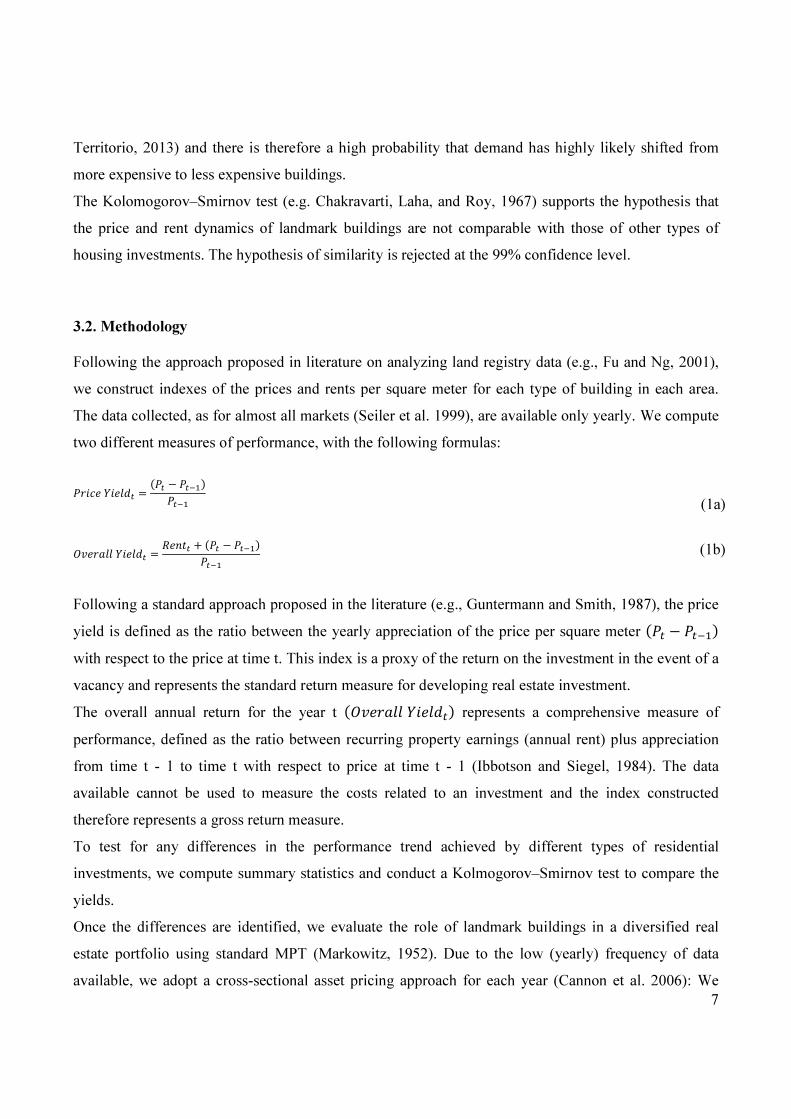
Following the approach proposed in literature on analyzing land registry data (e.g., Fu and Ng, 2001),

we construct indexes of the prices and rents per square meter for each type of building in each area.

The data collected, as for almost all markets (Seiler et al. 1999), are available only yearly. We compute

two different measures of performance, with the following formulas:

�� = �� − �� (1a)

� �� = �� + �� − �� (1b)

Following a standard approach proposed in the literature (e.g., Guntermann and Smith, 1987), the price

yield is defined as the ratio between the yearly appreciation of the price per square meter �� − ��

with respect to the price at time t. This index is a proxy of the return on the investment in the event of a

vacancy and represents the standard return measure for developing real estate investment.

The overall annual return for the year t �� represents a comprehensive measure of

performance, defined as the ratio between recurring property earnings (annual rent) plus appreciation

from time t - 1 to time t with respect to price at time t - 1 (Ibbotson and Siegel, 1984). The data

available cannot be used to measure the costs related to an investment and the index constructed

therefore represents a gross return measure.

To test for any differences in the performance trend achieved by different types of residential

investments, we compute summary statistics and conduct a Kolmogorov–Smirnov test to compare the

yields.

Once the differences are identified, we evaluate the role of landmark buildings in a diversified real

estate portfolio using standard MPT (Markowitz, 1952). Due to the low (yearly) frequency of data

available, we adopt a cross-sectional asset pricing approach for each year (Cannon et al. 2006): We

8

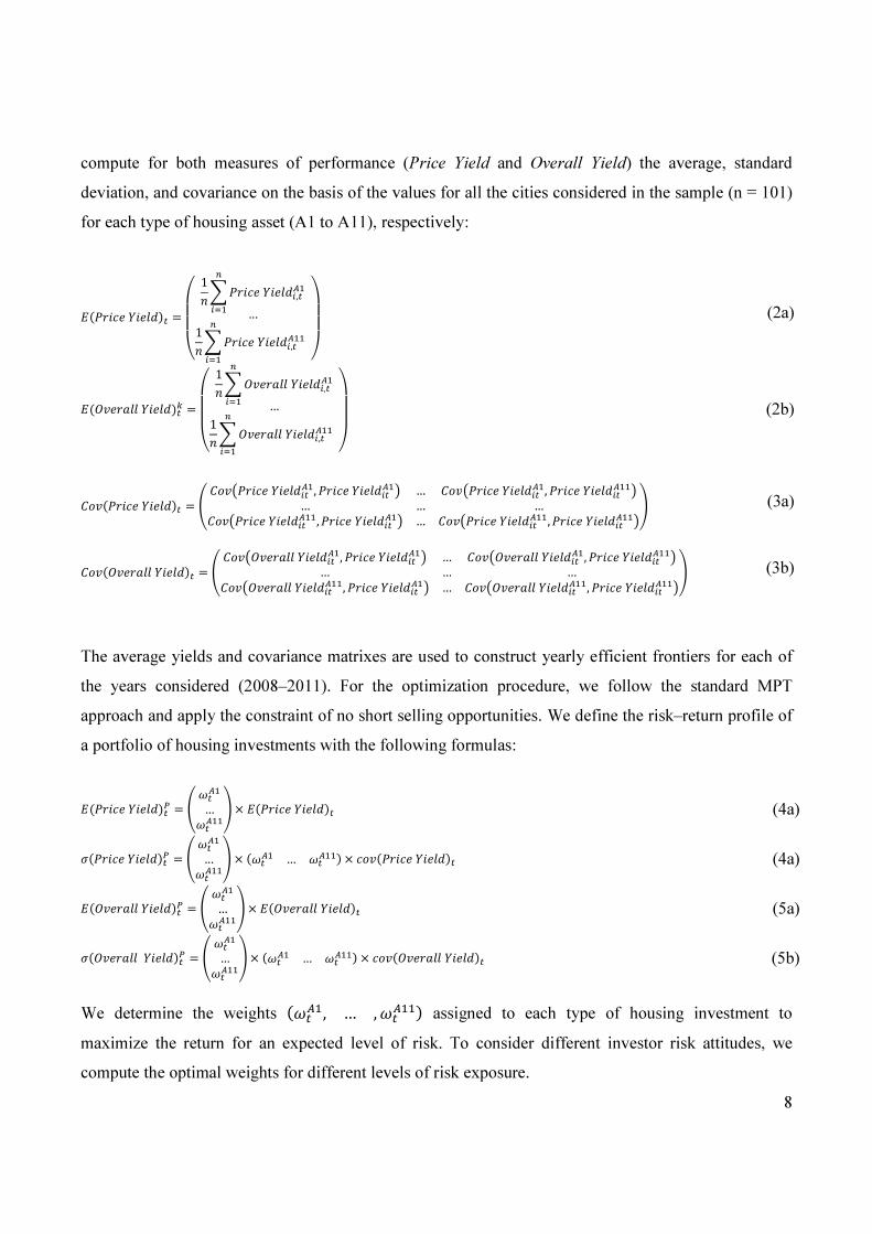
compute for both measures of performance (Price Yield and Overall Yield) the average, standard

deviation, and covariance on the basis of the values for all the cities considered in the sample (n = 101)

for each type of housing asset (A1 to A11), respectively:

�� =�� 1��,��

�� …

1��,��

��

�� (2a)

�(� ��)�� =

�� 1�� ,��

�� …

1�� ,��

��

�� (2b)

�� = �� ,�� … �� ,��… … …�� ,�� … �� ,�� (3a)

�� = � �� ,�� … �� ,��… … …�� ,�� … �� ,�� (3b)

The average yields and covariance matrixes are used to construct yearly efficient frontiers for each of

the years considered (2008–2011). For the optimization procedure, we follow the standard MPT

approach and apply the constraint of no short selling opportunities. We define the risk–return profile of

a portfolio of housing investments with the following formulas:

�(��)� = � ��

… ��

�× �� (4a)

!�� = � ��

… ��

� × �� … �

��× �� (4a)

�� = � ��

… ��

�× �� (5a)

!� �� = � ��

… ��

�× �� … �

�� × �� (5b)

We determine the weights ��

��, … ,��

�� assigned to each type of housing investment to

maximize the return for an expected level of risk. To consider different investor risk attitudes, we

compute the optimal weights for different levels of risk exposure.

9

To study the degree of efficiency of landmark buildings with respect to optimal investment portfolios,

we compute the distance of all solo portfolios with respect to the efficient frontier and compare the

distance from the efficient solution for the landmark portfolio with respect to the other specialized

portfolios. The degree of efficiency is defined as the minimum distance with respect to all the

portfolios on the efficient frontier. In other words,

"�#�� = $��%&&'&&()��

�− ��∗ �� + �!�� − !��∗ ��

…)��

�− ��∗ �� + �!�� − !��∗ ��

…)�� − ��∗ �� + �!�� − !��∗ ��*&&+&&,

(6a)

"�#�� = $��%&&'&&()��

�− �� ∗ �� + �!� �� − !� ��∗ ��

…)��

�− �� ∗ �� + �!� �� − !� ��∗ ��

…)�� − �� ∗ �� + �!� �� − !� ��∗ ��*&&+&&,

(6b)

where, for each year (t varies from 2008 to 2011) and for each type of residential investment (Aj varies

from A1 to A11), we compute n =100 distance measures of the solo portfolios with respect to the

efficient portfolios. The distance computed is a standard Euclidean measure of the square root of the

square of the horizontal differences �� − �� ∗ � and vertical differences

�� − �� ∗ � in the linear distances between the solo and efficient portfolios. We

consider the minimum distance to construct a proxy for the inefficiency of a concentrated portfolio

with respect to an optimized one for both Price Yield (formula 6a) and Overall Yield (formula 6b). The

analysis considers both a one-year time horizon and a multiple-year time horizon.

To study the role of landmark buildings in a diversification strategy, we also consider the composition

of portfolios on the efficient frontier and evaluate the role of different types of residential investments

on the basis of the risk–return profile of efficient portfolios. Summary statistics for the portfolio

composition for different levels of risk and return are presented for each year. The analysis considers

both a one-year time horizon and a multiple-year time horizon.

3.3. Results

Using data for rent and price per square meter, we compute two yearly indexes of performance (Price

Yield and Overall Yield) for 2007–2010 for all the residential types of buildings in the sample. Analysis

10

of the indexes computed for each type of residential property allows the identification of interesting

differences between landmark buildings and other types of residential investments (Table 3).


Considering the mean yield, the price yield achieved by landmark buildings is frequently higher than

for other housing investments. The results are even stronger when the overall yield is considered,

because, excluding 2007, performance is always higher with respect to other investment opportunities.

The overperformance achieved by landmark investments is partially offset by the higher risk exposure

of such investments. Landmark buildings are never the best investment solution to minimize risk for

any of the years considered because the risk assumed is normally double that of the safest solutions .

A comparison of yield distributions on the basis of Kolmogorov–Smirnov test cannot identify an

investment opportunity that has a distribution strictly comparable with that of landmark buildings. In

addition, the degree of similarity decreases over time, especially if we consider the overall trend.

The extra performance offered by landmark buildings demonstrates their usefulness as a solo portfolio

investment; however, to evaluate their usefulness in a diversified portfolio, one must also consider the

performance achieved by other types of residential investments. Analysis of the different housing

investments shows different degrees of correlations between the returns of different asset classes (Table

4).


The correlation between the returns of landmark buildings and other assets is normally higher when

overall yield is considered, due to the higher variability of price returns. During 2008–2010 the

correlation is usually high and statistically significant, whereas in 2011 the correlation decreases

significantly and is almost never statistically significant. This anomaly in 2011 can be explained on the

basis of the negative trend of transactions registered for the landmark sector due to the decrease in

demand for this type of expensive building.

To evaluate the relevance of landmark investments in a diversified portfolio, we construct the efficient

frontiers for each year for both price and overall yield measures and measure the distance of solo

portfolios with respect to the nearest efficient portfolio (those with more comparable risk–return

tradeoffs). The data are summarized in Table 5.

11


If we analyze the price dynamics, landmark buildings are not always on the efficient frontier. In 2010

and 2011 solo portfolios concentrated in other type of housing investments obtained a risk–return

tradeoff more similar to that of an efficient portfolio. When overall yield is considered, landmark

building solo portfolios are the only ones that are always on the efficient frontier; none of the other

concentrated portfolios achieves comparable results.

If we consider multiple time horizons, the results do not change significantly and the landmark building

solo portfolio is frequently an optimal investment strategy (Table 6).


Regarding price dynamics for a four-year time horizon, the landmark solo portfolio is always the

concentrated portfolio nearest to the frontier with respect to other investment opportunities, whereas

over a two- or three-year time horizon other solo portfolios may be more efficient than portfolios

investing only in landmark buildings. Lower returns for the investment strategy on two- and three-year

time horizons attain an investment strategy that includes 2011, the worst year in the period analyzed

for the landmark and all other upper class real estate investments (cf. Table 3).

Regarding overall yield, the distance with respect to the efficient frontier of solo landmark portfolios is

always zero and all other portfolios available are more distant from the efficient frontier. The distance

of the other investment opportunities with respect to the efficient portfolio normally increases with the

duration of the investment strategy (excluding low-income apartments).

To evaluate the usefulness of landmark buildings in a diversification strategy, we study the relation

between the number of real estate assets considered and the role of landmark buildings in the

composition of efficient portfolios (Figure 1).

[INSERT FIGURE 1 ABOVE THERE]

Significantly fewer types of assets were considered in 2008 and 2010 (between four and five) with

respect to 2011 (more than seven, on average). The anomaly related to the efficient portfolios

12

constructed in 2011 is related to the price performance dynamics that year, which show a significant

decrease of all the correlations between asset classes (cf. Table 4) and so an increase the usefulness of

more diversified portfolios in order to obtain the highest advantages related to a diversification

strategy. In examining the role of landmark buildings, our empirical analysis demonstrates that this

type of asset is usually useful in a diversification strategy, with the role of the asset increasing in

importance with the rise in risk assumed by the portfolio constructed.

To evaluate in more detail the relation between the risk of the portfolio constructed and the role of

landmark buildings, we classify efficient portfolios into deciles on the basis of portfolio risk and

compute statistics for each group of portfolios on only the role of landmark investments (Table 7).


If we compare the results obtained with the price return measure with those achieved with the overall

yield, the role of landmark buildings is greater for the latter on the basis of both the median and mean

values. If we consider overall yield, an efficient portfolio cannot be constructed without this asset (the

minimum is always higher than zero). Except for the price dynamics in 2011, the role of landmark

buildings grows with increases in risk and the highest-risk portfolios invest at least double in landmark

buildings with respect to the lowest-risk portfolios.

If we consider multiple time horizons, the results do not change significantly and the role of landmark

buildings in the efficient portfolios is always greater when overall yield is considered (Table 8).


Comparing the results obtained using the overall yield with those obtained with price performance, the

role of landmark buildings in efficient portfolios is greater for the former than for the latter. This

difference is relevant to both the mean and median values. The median and mean do not increase

proportionally with the increase in the duration of the investment strategy time horizon and the mean is

always higher than the median

Regarding the percentile distribution, excluding the price performance of the investment strategy for

2010 and 2011, the role of landmark buildings increases proportionally with the risk of the portfolio

constructed. Therefore, the relevance of landmark buildings is normally higher for riskier investors,

even for multiple-year time horizons.

13

4. Conclusion

Landmark buildings present price and rent dynamics that are not comparable with those of other types

of housing investments. The low correlation between the returns of this asset class with respect to those

of other types of residential investments could increase the usefulness of landmark buildings in the

construction of diversified portfolios. The standard MPT optimization usually includes landmark

buildings in the efficient portfolios and the role of this asset class increases with the rise in investor risk

tolerance. The results are relevant independently with respect to the time horizon of the investment

strategy and frequently a multiple-year time horizon magnifies the extra performance offered by

landmark investments compared to other housing investment opportunities.

Tax incentives have played an important role in transforming real estate investment trusts into one of

the main investors in landmark–trophy buildings in the commercial and office sectors (Getzedanner,

2004). The results presented in this paper support the hypothesis that landmark buildings represent an

interesting investment opportunity for the institutional investor, not only in the commercial and office

sectors but also in the residential sector. Due to the high number of specialized residential real estate

vehicles developed in the last years in both the United States and Europe (e.g., Colin, 2007), the

portfolio managers of such funds must consider the diversification benefits related to including

landmark buildings, as done by other portfolio managers not specialized in the residential sector.

Empirical evidence demonstrates a strict relation between maintenance costs or other expenses and

building appreciation/depreciation (e.g., Wilhelmsson, 2008). Therefore a more complete analysis

needs to consider not only gross returns (price or overall) but also net returns. Moreover, there is

evidence of a greater relevance of maintenance costs for historical buildings and, more generally, high-

quality standards buildings. Further investigation is thus necessary to evaluate if the extra gains related

to landmark investments still exist when net performance measures are considered.

Once the role of landmark buildings in a diversified housing portfolio is demonstrated, the next step

would be to test its usefulness in a diversified portfolio that includes other real estate asset classes (e.g.,

office, industrial, and commercial). Analysis of such diversification issue must consider the possibility

of including landmark buildings that are not classified as residential units and requires the construction

of indexes for price and/or overall performance that are comparable among different real estate asset

classes.

14

References

Agenzia del Territorio (2013), Rapporto Immobiliare 2012, available at http://www.agenziaterritorio.it/

(accessed 01/31/2013).

Appleyard D. Why Buildings Are Known: A Predictive Tool for Architects and Planners. Environment

and Behavior 1969; 1; 131-156.

Asabere PK, Hachey G, Grubaugh S., Architecture, Historic Zoning, and the value of Homes, Journal

of Real estate Finance and Economics 1989; 2; 181-195.

Asabere PK, Huffman FE. Historic Designation and Residential Market Values. Appraisal Journal

1994; 62; 396-401.

Block RL. Investing in REITs. John Wiley and Sons Inc.: Hoboken; 2011

Brown LJ, Li LH, Lusht K. A Note on Intracity Geographic Diversification of Real Estate Portfolios:

Evidence from Hong Kong. Journal of Real Estate Portfolio Management 2000; 6; 131-140.

Cannon S, Miller NG, Pandher GS. Risk and Return in the U.S. Housing Market: A Cross-Sectional

Asset-Pricing Approach. Real Estate Economics; 2006; 34; 519-552.

Chakravarti I., Laha R.G. and Roy L.J., (1967), Handbook of Methods of Applied Statistics, John Wiley

and Sons, New York.

Clark D, Herrin WE. Historical Preservation Districts and Home Sale Prices: Evidence from the

Sacramento Housing Market. Review of Regional Studies; 1997; 27; 29-48.

Coffin DA. The impact of Historic Districts on Residential Property Values. Eastern Economic Journal

1989; 15; 221-228.

Colin J. Private Investment in Rented Housing and the Role of REITS. European Journal of Housing

Policy 2007; 7; 383-400.

Coulson NE, Leichenko RM. The Internal and External Impact of Historical Designation on Property

Values. Journal of Real Estate Finance and Economics 2001; 23; 113-124.

Dixon WJ. Simplified Estimation from Censored Normal Samples. Annals of Mathematical Statistics 1960; 31; 385–391. Ford A. The Effect of Historic District Designation on Single-Family Home Prices. AREUEA Journal

1989; 17; 353-362.

Guntermann KL, Smith RL. Efficiency of the Market for Residential Real Estate. Land Economics

1987; 63; 34-45.

Fu Y, Ng LK. Market Efficiency and Return Statistics: Evidence from Real Estate and Stock Markets

Using a Present-Value Approach”, Real Estate Economics 2001; 29; 227–250.

15

Fuerst F, McAllister P, Murray C., Designer Buildings: An Evaluation of the Price Impacts of

Signature Architects, Real Estate & Planning Working Papers, 2009-10, Henley Business School,

Reading University available at http://centaur.reading.ac.uk/26999/ (accessed 07/01/2012)

Getzendanner VJ. Challenges in Representing “Trophy” Properties in Real Estate Tax Assessment

Appeals: A Tax Practitioner's Viewpoint. Journal of Property Tax Assessment & Administration 2004;

1; 87-98.

Goodman AC, Thibodeau TG. Housing Market Segmentation. Journal of Housing Economics 1998; 7;

121-143.

Hartzell D, Hekman J, Miles M. Diversification Categories in Investment Real Estate”, AREUEA

Journal 1986; 14; 230-254.

Hough DE, Kratz CG. Can “Good” Architecture Meet the Market Test?. Journal of Urban Economics

1983; 14; 40-54.

Hui ECM., Ng I, Lau OMF. Speculative bubbles in mass and luxury properties: an investigation of the

Hong Kong residential market. Construction Management and Economics 2011; 29; 781-793.

Ibbotson R.G. and Siegel L.B. (1984), “Real Estate Returns: A Comparison with Other Investments”,

AREUEA Journal, v. 12, i. 3, pp. 219-243.

Leichenko RM, Coulson NE, Listokin D. Historic Preservation and Residential Property Values: An

Analysis of Texas Cities. Urban Studies 2001; 38, 1973-1987.

Markowitz H. Portfolio selection. Journal of Finance 1952, 7, 77-91.

Moon SK, Lee SH, Min KM, Lee JS, Kim JH, Kim JJ. An Analysis of Landmark Impact Factors on

High-Rise Residential Buildings Value Assessment. International Journal of Strategic Property

Management 2010; 14; 105-120.

Narwold A, Sandy J, Tu C. Historic Designation and Residential Property Values. International Real

Estate Review 2008; 11; 83-95.

Noonan DS. Finding an Impact of Preservation Policies: Price Effects of Historic Landmarks on

Attached Homes in Chicago, 1990-1999. Economic Development Quarterly 2007; 21; 17-33.

Noonan DS, Krupka DJ. Determinants of Historic and Cultural Landmark Designation: Why We

Preserve what We Preserve. Journal of Cultural Economics 2010; 34; 1-26.

Noonan DS, Krupka DJ. Making—or Picking—Winners: Evidence of Internal and External Price

Effects in Historic Preservation Policies. Real Estate Economics 2011; 39; 379-407.

Pagliari JL, Webb JR, Del Casino JJ. Applying MPT to Institutional Real Estate Portfolios: The Good,

the Bad and the Uncertain. Journal of Real Estate Portfolio Management 1995; 1, 67-88.

16

Schaeffer PV, Millerick CA. The Impact of Historic District Designation on Property Values: An

Empirical Study. Economic Development Quarterly 1991; 5; 301-312.

Seiler, M.J., Webb J.R., Myer FCN. Diversification Issues in Real Estate Investment. Journal of Real

Estate Literature 1999; 7; 163-179.

Wilhelmsson, M. House Price Depreciation Rates and Level of Maintenance. Journal of Housing Economics 2008; 17; 88-101. Zahirovic-Herbert V, Chatterjee S. What is the Value of a Name? Conspicuous Consumption and

House Prices. Journal of Real Estate Finance and Economics 2011, 33; 105-125.

Zahirovic-Herbert V, Chatterjee S. Historic Preservation and Residential Property Values: Evidence

from Quantile Regression. Urban Studies, 2012; 49; 369-382.

Appendix

On the basis of the current law defined in 1939 (the so called “Nuovo Catasto Edilizio Urbano”), Italian houses are classified in one of the following categories: Type A1 – Luxury house: Real estate units places in highly requested areas characterized by construction standards, technology and refurbishment higher that the average for the residential sector. Type A2 - High income apartment: Real estate units characterized by construction standards, technology and refurbishment coherent with the local area demand. Type A3 - Middle income apartment: Real estate units constructed with under the average quality standards and technology limited to essential. Type A4 – Low income apartment: Real estate units constructed with lower quality standards and technology limited to essential. Type A5 – Economy apartment: Real estate units constructed with the lowest quality standards. Type A6 – Rural Houses: Real estate units constructed for agriculture purposed and used also as an house by the owners. Type A7 – Maison: Independent real estate units characterized by construction standards, technology and refurbishment coherent with the local area demand or under the average. Type A8 – Independent real estate units places in highly requested areas characterized by construction standards, technology and refurbishment higher that the average for the residential sector. Type A9 – Castles or villas characterized by outstanding / unique features with respect to other building available for the same type of households. Type A11 – Crude building: Mountain Dew, Shack, etc..

Figure 1. The role of the landmark investment in the efficient portfolios

The figure presents the role of the landmark buildings in the efficient frontier for portfolios with different level of risk. Data

are presented for both price and overall yield and.

Price Yield Overall Yield

2008

*2009

2010

2011

Source: Agenzia del territorio data processed by the author

Table 1. Sample description

Overall sample – number of residential units*

2008 2009 2010 2011

Landmark building (A9) 2,430 2,451 2,463 2519

Luxury apartment (A1) 36,732 36,385 36,291 36154

High income apartment (A2) 10,817,919 11,093,017 11,330,912 11,580,391

Middle income apartment (A3) 11,431,139 11,637,545 11,821,498 12,061,170

Low income apartment (A4) 5,673,259 5,672,572 5,665,910 5,683,426

Economy apartment (A5) 1,132,215 1,098,443 1,068,257 1,035,957

Rural Houses (A6) 859,111 833,421 808,526 782,429

Maison (A7) 1,993,667 2,058,375 2,118,819 2,193,650

Manor (A8) 34,288 34,427 34,628 35,007

Crude Building (A11) 17,086 17,435 18,061 18,696

Landmark buildings

2008 2009 2010 2011

N° of Landmark buildings in North-west 1690 1691 1693 1703

N° of Landmark buildings in North-east 96 97 97 99

N° of Landmark buildings in Center 513 553 563 604

N° of Landmark buildings in South and Islands 131 110 110 113

N° of cities with landmark buildings 86 86 86 86

N° of cities without landmark buildings 15 15 15 15

Mean landmark buildings for each city 24 24 24 25

Min landmark buildings for each city 0 0 0 0

Max landmark buildings for each city 512 505 503 502 Source: Agenzia del territorio data processed by the author

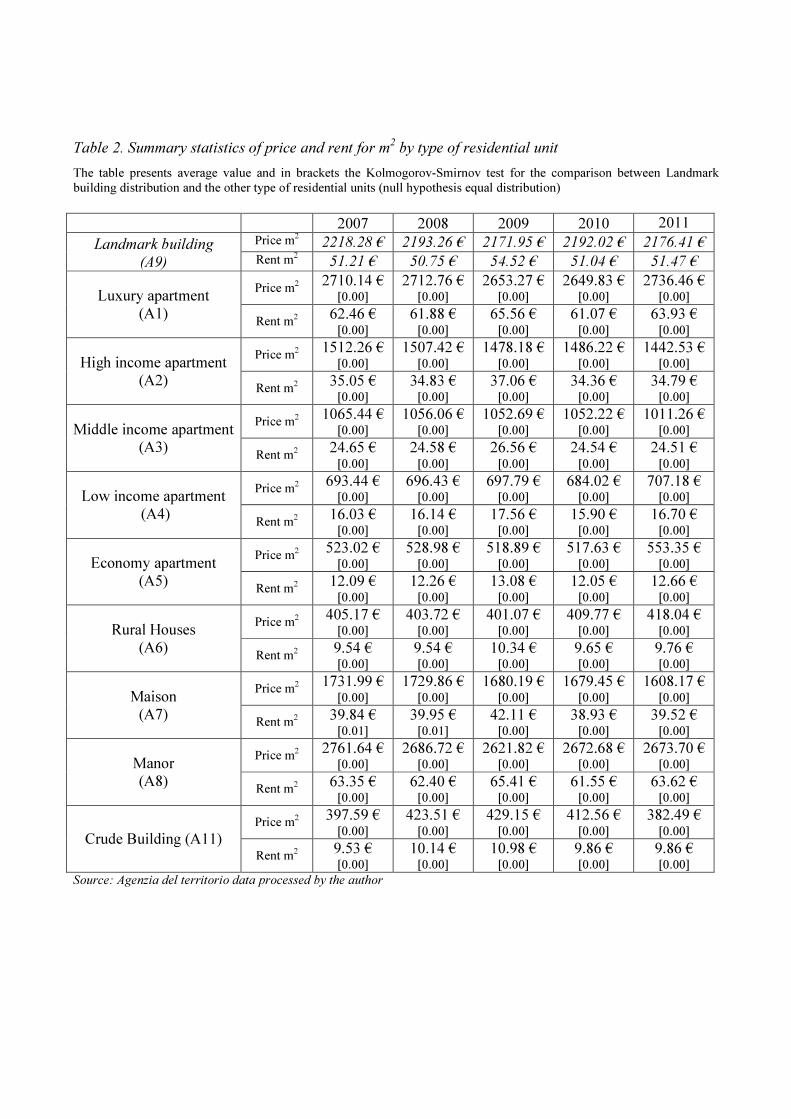
Table 2. Summary statistics of price and rent for m2 by type of residential unit

The table presents average value and in brackets the Kolmogorov-Smirnov test for the comparison between Landmark

building distribution and the other type of residential units (null hypothesis equal distribution)

2007 2008 2009 2010 2011

Landmark building

(A9)

Price m2 2218.28 € 2193.26 € 2171.95 € 2192.02 € 2176.41 €

Rent m2 51.21 € 50.75 € 54.52 € 51.04 € 51.47 €

Luxury apartment

(A1)

Price m2

2710.14 € [0.00]

2712.76 € [0.00]

2653.27 € [0.00]

2649.83 € [0.00]

2736.46 € [0.00]

Rent m2

62.46 € [0.00]

61.88 € [0.00]

65.56 € [0.00]

61.07 € [0.00]

63.93 € [0.00]

High income apartment

(A2)

Price m2

1512.26 € [0.00]

1507.42 € [0.00]

1478.18 € [0.00]

1486.22 € [0.00]

1442.53 € [0.00]

Rent m2

35.05 € [0.00]

34.83 € [0.00]

37.06 € [0.00]

34.36 € [0.00]

34.79 € [0.00]

Middle income apartment (A3)

Price m2

1065.44 € [0.00]

1056.06 € [0.00]

1052.69 € [0.00]

1052.22 € [0.00]

1011.26 € [0.00]

Rent m2

24.65 € [0.00]

24.58 € [0.00]

26.56 € [0.00]

24.54 € [0.00]

24.51 € [0.00]

Low income apartment

(A4)

Price m2

693.44 € [0.00]

696.43 € [0.00]

697.79 € [0.00]

684.02 € [0.00]

707.18 € [0.00]

Rent m2

16.03 € [0.00]

16.14 € [0.00]

17.56 € [0.00]

15.90 € [0.00]

16.70 € [0.00]

Economy apartment

(A5)

Price m2

523.02 € [0.00]

528.98 € [0.00]

518.89 € [0.00]

517.63 € [0.00]

553.35 € [0.00]

Rent m2

12.09 € [0.00]

12.26 € [0.00]

13.08 € [0.00]

12.05 € [0.00]

12.66 € [0.00]

Rural Houses

(A6)

Price m2

405.17 € [0.00]

403.72 € [0.00]

401.07 € [0.00]

409.77 € [0.00]

418.04 € [0.00]

Rent m2

9.54 € [0.00]

9.54 € [0.00]

10.34 € [0.00]

9.65 € [0.00]

9.76 € [0.00]

Maison

(A7)

Price m2

1731.99 € [0.00]

1729.86 € [0.00]

1680.19 € [0.00]

1679.45 € [0.00]

1608.17 € [0.00]

Rent m2

39.84 € [0.01]

39.95 € [0.01]

42.11 € [0.00]

38.93 € [0.00]

39.52 € [0.00]

Manor

(A8)

Price m2

2761.64 € [0.00]

2686.72 € [0.00]

2621.82 € [0.00]

2672.68 € [0.00]

2673.70 € [0.00]

Rent m2

63.35 € [0.00]

62.40 € [0.00]

65.41 € [0.00]

61.55 € [0.00]

63.62 € [0.00]

Crude Building (A11) Price m

2

397.59 € [0.00]

423.51 € [0.00]

429.15 € [0.00]

412.56 € [0.00]

382.49 € [0.00]

Rent m2

9.53 € [0.00]

10.14 € [0.00]

10.98 € [0.00]

9.86 € [0.00]

9.86 € [0.00]


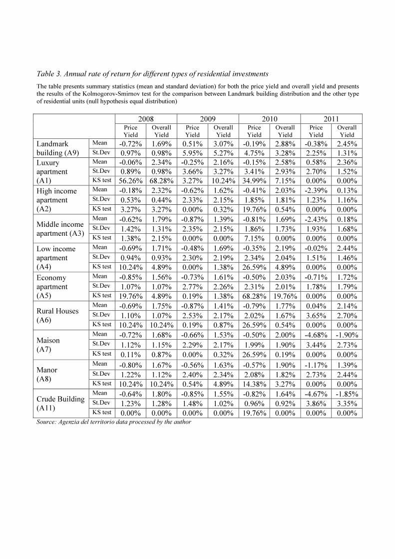
Table 3. Annual rate of return for different types of residential investments

The table presents summary statistics (mean and standard deviation) for both the price yield and overall yield and presents

the results of the Kolmogorov-Smirnov test for the comparison between Landmark building distribution and the other type

of residential units (null hypothesis equal distribution)

2008 2009 2010 2011 Price

Yield

Overall

Yield

Price

Yield

Overall

Yield

Price

Yield

Overall

Yield

Price

Yield

Overall

Yield

Landmark

building (A9)

Mean -0.72% 1.69% 0.51% 3.07% -0.19% 2.88% -0.38% 2.45% St.Dev 0.97% 0.98% 5.95% 5.27% 4.75% 3.28% 2.25% 1.31%

Luxury

apartment

(A1)

Mean -0.06% 2.34% -0.25% 2.16% -0.15% 2.58% 0.58% 2.36% St.Dev 0.89% 0.98% 3.66% 3.27% 3.41% 2.93% 2.70% 1.52% KS test 56.26% 68.28% 3.27% 10.24% 34.99% 7.15% 0.00% 0.00%

High income

apartment (A2)

Mean -0.18% 2.32% -0.62% 1.62% -0.41% 2.03% -2.39% 0.13% St.Dev 0.53% 0.44% 2.33% 2.15% 1.85% 1.81% 1.23% 1.16% KS test 3.27% 3.27% 0.00% 0.32% 19.76% 0.54% 0.00% 0.00%

Middle income

apartment (A3)


Low income

apartment

(A4)


Economy

apartment

(A5)


Rural Houses

(A6)

Mean -0.69% 1.75% -0.87% 1.41% -0.79% 1.77% 0.04% 2.14% St.Dev 1.10% 1.07% 2.53% 2.17% 2.02% 1.67% 3.65% 2.70% KS test 10.24% 10.24% 0.19% 0.87% 26.59% 0.54% 0.00% 0.00%

Maison

(A7)

Mean -0.72% 1.68% -0.66% 1.53% -0.50% 2.00% -4.68% -1.90% St.Dev 1.12% 1.15% 2.29% 2.17% 1.99% 1.90% 3.44% 2.73% KS test 0.11% 0.87% 0.00% 0.32% 26.59% 0.19% 0.00% 0.00%

Manor

(A8)


Crude Building

(A11)

Mean -0.64% 1.80% -0.85% 1.55% -0.82% 1.64% -4.67% -1.85% St.Dev 1.23% 1.28% 1.48% 1.02% 0.96% 0.92% 3.86% 3.35% KS test 0.00% 0.00% 0.00% 0.00% 19.76% 0.00% 0.00% 0.00%


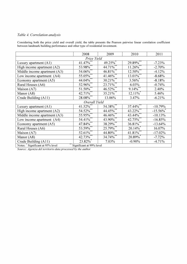
Table 4. Correlation analysis

Considering both the price yield and overall yield, the table presents the Pearson pairwise linear correlation coefficient

between landmark building performance and other type of residential investment.

2008 2009 2010 2011

Price Yield

Luxury apartment (A1) 41.47%** 49.25%* 29.89%** -7.23%

High income apartment (A2) 53.98%** 44.71%** 11.26%** -2.70%

Middle income apartment (A3) 54.06%** 46.81%

** 12.50%

** -4.12%

Low income apartment (A4) 55.05%** 41.46%

** 13.01%

** -8.68%

Economy apartment (A5) 44.04%** 30.21%

** 3.56%

* -8.18%

Rural Houses (A6) 52.96%** 23.71%

** 6.03% -0.74%

Maison (A7) 51.50%** 46.52%** 9.14%** 2.40%

Manor (A8) 42.71%** 35.21%

** 12.11%

* 5.46%

Crude Building (A11) 28.08%** 13.06% 3.47% -6.21%

Overall Yield

Luxury apartment (A1) 41.52%** 54.38%

** 37.44%

** -10.79%

High income apartment (A2) 54.52%** 44.45%

** 43.22%

** -15.56%

*

Middle income apartment (A3) 55.95%** 46.46%** 43.44%** -10.13%

Low income apartment (A4) 54.41%** 43.90%

** 42.75%

** -16.85%

Economy apartment (A5) 47.84%** 38.29%

** 36.81%

** -13.64%

Rural Houses (A6) 53.59%** 25.79%

** 20.14%

* 16.07%

Maison (A7) 52.61%** 44.80%

** 41.81%

** -17.02%

Manor (A8) 42.73%** 34.74%** 20.89%* -7.72%

Crude Building (A11) 23.82%* 7.03% -0.90% -4.71% Notes:

* Significant at 95% level

** Significant at 99% level


Table 5. Statistics on the distance between efficient frontiers and type of investments

Considering both price yield and overall yield, the table presents the minimum distance between the efficient frontier and

the solo-portfolio investment constructed on different types of residential units.


2008 2009 2010 2011 2008 2009 2010 2011

Landmark building (A9) 0.00% 0.00% 1.34% 0.81% 0.00% 0.00% 0.00% 0.00%

Luxury apartment (A1) 0.46% 0.28% 0.00% 0.26% 0.40% 0.32% 0.25% 0.23%

High income apartment (A2) 0.17% 0.28% 0.04% 1.32% 0.22% 0.49% 0.34% 1.44%

Middle income apartment (A3) 0.34% 0.52% 0.42% 1.74% 0.43% 0.71% 0.62% 1.64%

Low income apartment (A4) 0.29% 0.14% 0.08% 0.00% 0.29% 0.44% 0.29% 0.16%

Economy apartment (A5) 0.32% 0.51% 0.23% 0.73% 0.39% 0.53% 0.43% 0.88%

Rural Houses (A6) 0.46% 0.58% 0.45% 1.74% 0.39% 0.69% 0.52% 1.42%

Maison (A7) 0.21% 0.30% 0.15% 4.44% 0.28% 0.58% 0.41% 3.95%

Manor (A8) 0.35% 0.24% 0.24% 1.67% 0.37% 0.54% 0.47% 1.55%

Crude Building (A11) 0.20% 0.10% 0.12% 4.70% 0.09% 0.03% 0.15% 4.27%


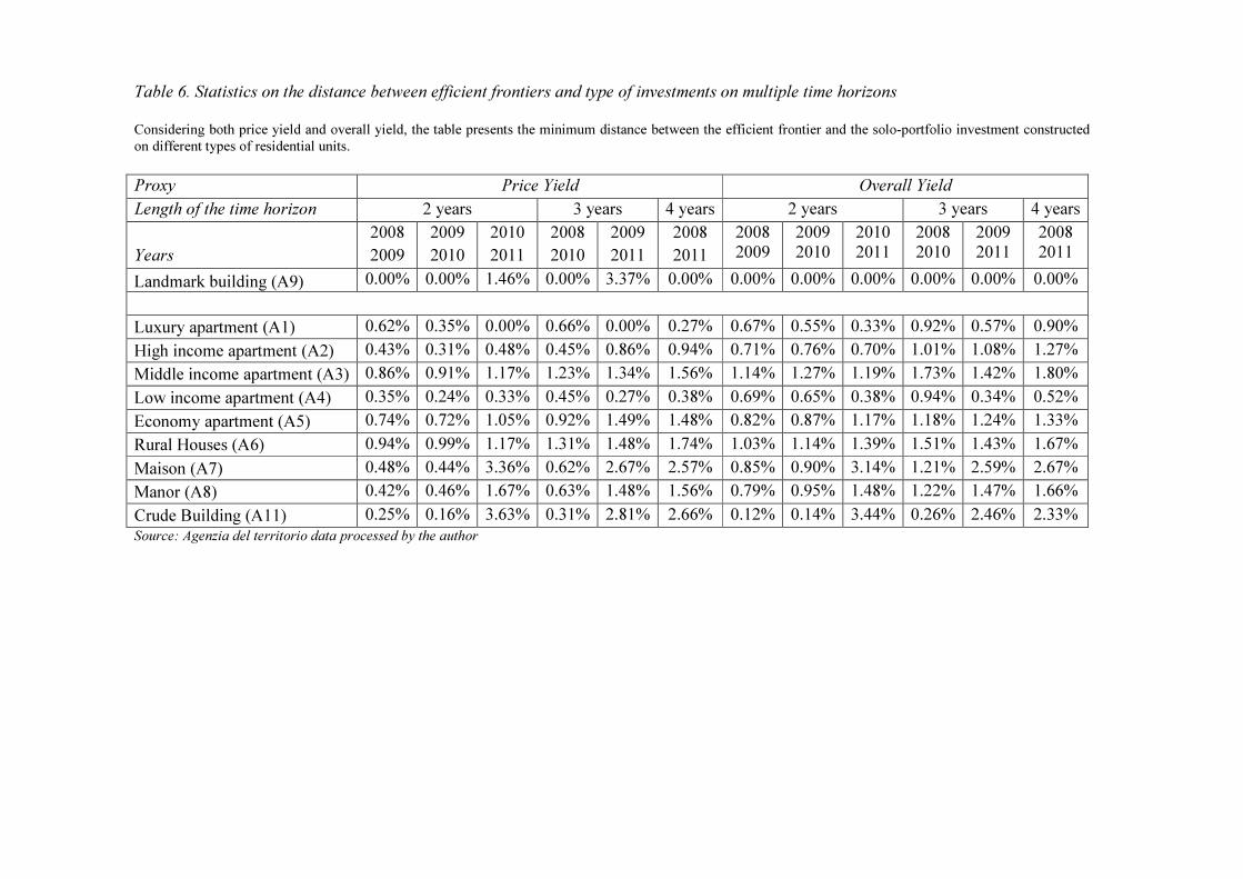
Table 6. Statistics on the distance between efficient frontiers and type of investments on multiple time horizons

Considering both price yield and overall yield, the table presents the minimum distance between the efficient frontier and the solo-portfolio investment constructed

on different types of residential units.

Proxy Price Yield Overall Yield

Length of the time horizon 2 years 3 years 4 years 2 years 3 years 4 years

Years

2008

2009

2009

2010

2010

2011

2008

2010

2009

2011

2008

2011

2008

2009

2009

2010

2010

2011

2008

2010

2009

2011

2008

2011

Landmark building (A9) 0.00% 0.00% 1.46% 0.00% 3.37% 0.00% 0.00% 0.00% 0.00% 0.00% 0.00% 0.00%

Luxury apartment (A1) 0.62% 0.35% 0.00% 0.66% 0.00% 0.27% 0.67% 0.55% 0.33% 0.92% 0.57% 0.90%

High income apartment (A2) 0.43% 0.31% 0.48% 0.45% 0.86% 0.94% 0.71% 0.76% 0.70% 1.01% 1.08% 1.27%

Middle income apartment (A3) 0.86% 0.91% 1.17% 1.23% 1.34% 1.56% 1.14% 1.27% 1.19% 1.73% 1.42% 1.80%

Low income apartment (A4) 0.35% 0.24% 0.33% 0.45% 0.27% 0.38% 0.69% 0.65% 0.38% 0.94% 0.34% 0.52%

Economy apartment (A5) 0.74% 0.72% 1.05% 0.92% 1.49% 1.48% 0.82% 0.87% 1.17% 1.18% 1.24% 1.33%

Rural Houses (A6) 0.94% 0.99% 1.17% 1.31% 1.48% 1.74% 1.03% 1.14% 1.39% 1.51% 1.43% 1.67%

Maison (A7) 0.48% 0.44% 3.36% 0.62% 2.67% 2.57% 0.85% 0.90% 3.14% 1.21% 2.59% 2.67%

Manor (A8) 0.42% 0.46% 1.67% 0.63% 1.48% 1.56% 0.79% 0.95% 1.48% 1.22% 1.47% 1.66%

Crude Building (A11) 0.25% 0.16% 3.63% 0.31% 2.81% 2.66% 0.12% 0.14% 3.44% 0.26% 2.46% 2.33%


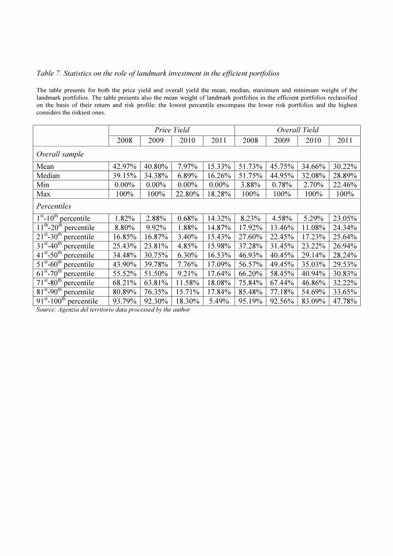
Table 7. Statistics on the role of landmark investment in the efficient portfolios

The table presents for both the price yield and overall yield the mean, median, maximum and minimum weight of the

landmark portfolios. The table presents also the mean weight of landmark portfolios in the efficient portfolios reclassified

on the basis of their return and risk profile: the lowest percentile encompass the lower risk portfolios and the highest

considers the riskiest ones.


2008 2009 2010 2011 2008 2009 2010 2011

Overall sample

Mean 42.97% 40.80% 7.97% 15.33% 51.73% 45.75% 34.66% 30.22%

Median 39.15% 34.38% 6.89% 16.26% 51.75% 44.95% 32.08% 28.89%

Min 0.00% 0.00% 0.00% 0.00% 3.88% 0.78% 2.70% 22.46%

Max 100% 100% 22.80% 18.28% 100% 100% 100% 100%

Percentiles

1st-10

th percentile 1.82% 2.88% 0.68% 14.32% 8.23% 4.58% 5.29% 23.05%

11th

-20th

percentile 8.80% 9.92% 1.88% 14.87% 17.92% 13.46% 11.08% 24.34%

21st-30th percentile 16.85% 16.87% 3.40% 15.43% 27.60% 22.45% 17.23% 25.64%

31st-40

th percentile 25.43% 23.81% 4.85% 15.98% 37.28% 31.45% 23.22% 26.94%

41st-50

th percentile 34.48% 30.75% 6.30% 16.53% 46.93% 40.45% 29.14% 28.24%

51st-60

th percentile 43.90% 39.78% 7.76% 17.09% 56.57% 49.45% 35.03% 29.53%

61st-70

th percentile 55.52% 51.50% 9.21% 17.64% 66.20% 58.45% 40.94% 30.83%

71st-80

th percentile 68.21% 63.81% 11.58% 18.08% 75.84% 67.44% 46.86% 32.22%

81st-90th percentile 80.89% 76.35% 15.71% 17.84% 85.48% 77.18% 54.69% 33.65%

91st-100

th percentile 93.79% 92.30% 18.30% 5.49% 95.19% 92.56% 83.09% 47.78%


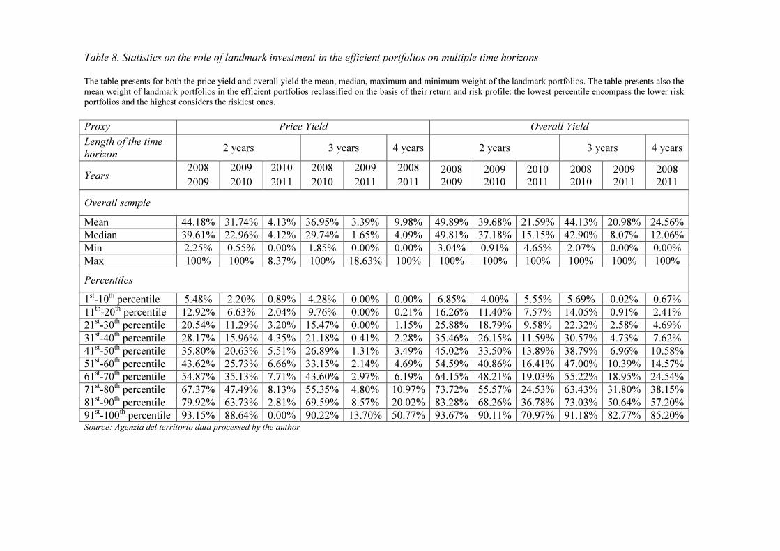
Table 8. Statistics on the role of landmark investment in the efficient portfolios on multiple time horizons

The table presents for both the price yield and overall yield the mean, median, maximum and minimum weight of the landmark portfolios. The table presents also the

mean weight of landmark portfolios in the efficient portfolios reclassified on the basis of their return and risk profile: the lowest percentile encompass the lower risk

portfolios and the highest considers the riskiest ones.

Proxy Price Yield Overall Yield

Length of the time

horizon 2 years 3 years 4 years 2 years 3 years 4 years

Years 2008

2009

2009

2010

2010

2011

2008

2010

2009

2011

2008

2011

2008

2009

2009

2010

2010

2011

2008

2010

2009

2011

2008

2011

Overall sample

Mean 44.18% 31.74% 4.13% 36.95% 3.39% 9.98% 49.89% 39.68% 21.59% 44.13% 20.98% 24.56%

Median 39.61% 22.96% 4.12% 29.74% 1.65% 4.09% 49.81% 37.18% 15.15% 42.90% 8.07% 12.06%

Min 2.25% 0.55% 0.00% 1.85% 0.00% 0.00% 3.04% 0.91% 4.65% 2.07% 0.00% 0.00%

Max 100% 100% 8.37% 100% 18.63% 100% 100% 100% 100% 100% 100% 100%

Percentiles

1st-10th percentile 5.48% 2.20% 0.89% 4.28% 0.00% 0.00% 6.85% 4.00% 5.55% 5.69% 0.02% 0.67%

11th

-20th

percentile 12.92% 6.63% 2.04% 9.76% 0.00% 0.21% 16.26% 11.40% 7.57% 14.05% 0.91% 2.41%

21st-30

th percentile 20.54% 11.29% 3.20% 15.47% 0.00% 1.15% 25.88% 18.79% 9.58% 22.32% 2.58% 4.69%

31st-40

th percentile 28.17% 15.96% 4.35% 21.18% 0.41% 2.28% 35.46% 26.15% 11.59% 30.57% 4.73% 7.62%

41st-50

th percentile 35.80% 20.63% 5.51% 26.89% 1.31% 3.49% 45.02% 33.50% 13.89% 38.79% 6.96% 10.58%

51st-60

th percentile 43.62% 25.73% 6.66% 33.15% 2.14% 4.69% 54.59% 40.86% 16.41% 47.00% 10.39% 14.57%

61st-70th percentile 54.87% 35.13% 7.71% 43.60% 2.97% 6.19% 64.15% 48.21% 19.03% 55.22% 18.95% 24.54%

71st-80

th percentile 67.37% 47.49% 8.13% 55.35% 4.80% 10.97% 73.72% 55.57% 24.53% 63.43% 31.80% 38.15%

81st-90

th percentile 79.92% 63.73% 2.81% 69.59% 8.57% 20.02% 83.28% 68.26% 36.78% 73.03% 50.64% 57.20%

91st-100

th percentile 93.15% 88.64% 0.00% 90.22% 13.70% 50.77% 93.67% 90.11% 70.97% 91.18% 82.77% 85.20%


Landmark Buildings and Diversification Opportunities in ... ANNUAL MEETINGS/2013-… · Landmark...

Documents

Transcript of Landmark Buildings and Diversification Opportunities in ... ANNUAL MEETINGS/2013-… · Landmark...