
VERIFICATION OF LAMINAR AND TRANSITIONAL FLOW SIMULATIONS ...
Upload
leslie-quintanaCategory
view
213download
1description

J. Non-Newtonian Fluid Mech. 128 (2005) 172–184
Laminar transitional and turbulent flow of yield stress fluid in a pipe
J. Peixinhoa,b,∗, C. Nouara, C. Desaubrya, B. Theronb
a LEMTA, Laboratoire d’Energetique et de M´ecanique Th´eorique et Appliqu´ee, UMR 7563,2, avenue de la Forˆet de Haye, BP 160, 54 504 Vandœuvre-l`es-Nancy Cedex, France
b Schlumberger 1, rue Becquerel, 92 140 Clamart Cedex, France
Received 6 November 2003; received in revised form 21 March 2005; accepted 29 March 2005
Abstract
This paper presents an experimental study of the laminar, transitional and turbulent flows in a cylindrical pipe facility (5.5 m length and30 mm inner diameter). Three fluids are used: a yield stress fluid (aqueous solution of 0.2% Carbopol), a shear thinning fluid (aqueoussolution of 2% CMC) without yield stress and a Newtonian fluid (glucose syrup) as a reference fluid. Detailed rheological properties (simpleshear viscosity and first normal stress difference) are presented. The flow is monitored using pressure and (laser Doppler) axial velocitymeasurements. The critical Reynolds numbers from which the experimental results depart from the laminar solution are determined andc nsition fora hilei ole sectionb ids. Finally,a ares©
1
tTtcurB
cidnr
eM
e, re-henulk
liter-on
log-inen-
then
med
-ap-from
isard
uille
0d
ompared with phenomenological criteria. The results show that the yield stress contribute to stabilize the flow. Concerning the trayield stress fluid it has been observed an increase of the root mean square (rms) of the axial velocity outside a region around the axis w
t remains at a laminar level inside this region. Then, with increasing the Reynolds number, the fluctuations increase in the whecause of the apparition of turbulent spots. The time trace of the turbulent spots are presented and compared for the different fludescription of the turbulent flow is presented and shows that thermsaxial velocity profile for the Newtonian and non-Newtonian fluids
imilar except in the vicinity of the wall where the turbulence intensity is larger for the non-Newtonian fluids.2005 Elsevier B.V. All rights reserved.
. Introduction
The present study deals with the laminar, transitional andurbulent flow of a viscoplastic fluid in a cylindrical pipe.he origin of this study comes from the oil industry, where
he control of processes requires the knowledge of the flowharacteristics in ducts for different flow rates. The fluidssed are shear thinning and possess a yield stress,τY. Theirheological behaviour is usually described by the Herschel–ulkley model.In laminar fully developed flow, the axial velocity profile is
haracterized by a plug zone around the axis of the duct mov-ng with the maximum velocity. The radiusrp of the plug zoneepends on the power law indexn and the Herschel–BulkleyumberHb also called generalized Bingham numberB (theatio of the yield stress to a nominal viscous shear stress).
∗ Corresponding author. Present address: Manchester Center for Nonlin-ar Dynamics, The University of Manchester, Brunswick Road, Manchester13 9PL, UK.E-mail address:[email protected] (J. Peixinho).
With increasing the flow rate, the viscous forces increasducing the plug zone radius. The axial velocity profile is tless flat and the ratio of the plug zone velocity to the bvelocity increases. These results are well known in theature (Bird et al.[1]) and will be presented briefly in Secti4.
Concerning the critical Reynolds number, phenomenoical criteria ([2–7]) developed in the 50’s are widely usedindustrial applications. A general approach is to use a dimsionless ratio of two physical quantities, which controlstability of the flow. The critical value of this ratio is knowor can be calculated for Newtonian fluid. It is then assuthat this value is the same for all the viscous fluids.Fig. 1presents the evolution of the critical Reynolds number,Re′
cbased on the definition of Metzner and Reed[2], as a function of Hb. A divergence between the different criteriapears when rheological behaviour departs significantlyNewtonian behaviour.
From a theoretical point of view, the main difficultyto deal with the unyielded plug zone. Nouar and Friga[8] perform a non-linear stability analysis of plane Poise
377-0257/$ – see front matter © 2005 Elsevier B.V. All rights reserved.oi:10.1016/j.jnnfm.2005.03.008

J. Peixinho et al. / J. Non-Newtonian Fluid Mech. 128 (2005) 172–184 173
Nomenclature
a dimensionless plug size(= rp
R= τY
τw
)
B Bingham number(= τY
K(U/R)
)E dimensionless spectrum energyD pipe diameter (m)
f friction factor(= 2τw
ρU2
)fN friction factor for a Newtonian fluid
Hb Herschel–Bulkley number(= τY
K(U/R)n
)k constant in the Cross model (s)k′ generalized consistency (Pa s−n′
)K constant in the Herschel–Bulkley model
(Pa sn)Le entrance length (m)Lp length between the two pressure tappings (m)m power law exponent in the Cross modeln power law exponent in the Oswald and
Herschel–Bulkleyn′ generalized index flow behaviorp pressure (Pa)r radial location within pipe (m)rp radius of constant velocity plastic plug (m)R pipe radius (m)Re Reynolds number for Newtonian fluidRec critical Reynolds number for Newtonian fluid
Re′ generalized Reynolds number
(= ρU2−n′
Rn′
8n′−1k′
)
Re′c critical generalized Reynolds number
Reg Reynolds number
(= ρU2−n′
Rn′K
)
Rew wall Reynolds number(= ρUD
µw
)t time (s)u axial velocity (m/s)u′ axial velocity fluctuation (m/s)u′
c centreline axial velocity fluctuation (m/s)uc centreline axial velocity (m/s)
uτ friction velocity(=
√τwρ
)
u+ dimensionless velocity(= u
uτ
)U bulk velocity (m/s)y distance from the wall (m)
yτ friction distance from the wall(= µw
ρuτ
)
y+ dimensionless distance from the wall(= y
yτ
)y+
c centreline dimensionless distance from thewall
z longitudinal coordinate (m)
Greek lettersγ shear rate (s−1)µ fluid viscosity (kg m−1 s−1)
µ0 zero shear stress dynamic viscosity in the Crossmodel (kg m−1 s−1)
µw dynamic viscosity of the fluid at pipe wall(kg m−1 s−1)
µ∞ infinite dynamic viscosity in the Cross model(kg m−1 s−1)
ρ fluid density (kg m−3)τ shear stress (Pa)τY yield stress (Pa)τw wall shear stress (Pa)
flow and Hagen–Poiseuille flow of a Bingham fluid, using theenergy method, bounds for non-linear stability are derived.Although very weak, these bounds provide a first rigorousdemonstration that the Poiseuille flow of a Bingham fluid ismore stable than its Newtonian counterpart. Frigaard et al.[9]perform a linear stability analysis of plane Poiseuille flow ofa Bingham fluid via Orr–Sommerfeld equations. The numer-ical results show that the critical Reynolds number based onthe plastic viscosity increase with increasingB andRec(B)is practically linear for largeB. Comparing, the theoreticalbounds (linear and non-linear) with the phenomenologicalcriteria shows that only Hanks criterion[3] is compatible withthe theoretical bounds for largeB. However, for low values ofB (the most practical application) it is not possible to deter-mine theoretically which of them is the best criterion. In thissituation, the only way to determine, which criteria is most
F lkleyn eedcci eH
ig. 1. Critical Reynolds number as a function of the Herschel–Buumber: comparison between different criteria—‘MR’ Metzner and Rriterion[2]; ‘H’ Hedstrom criterion[4], ‘R’ Ryan and Johnson[5] or Hanksriterion [3]; ‘M’ Mishra criterion [6]; ‘S’ Slatter criterion[7]. ‘5’ and ‘1’
ndicaten = 0.5 andn = 1, respectively (n is the power law index of therschel–Bulkley model).

174 J. Peixinho et al. / J. Non-Newtonian Fluid Mech. 128 (2005) 172–184
applicable is to compare with experimental results. In addi-tion, the linear and non-linear stability analyses for Binghamfluid give little insight into the actual transition mechanisms.
From an experimental point of view, the process wherebyturbulence arises is still not understood. The transition is verysensitive on the inlet conditions. Indeed, careful conditionscan permit laminar flow for very large Reynolds numbers.Using careful entrance conditions (a settling chamber and asmooth contraction at the entrance of the pipe) and Newto-nian (water) and non-Newtonian fluids (dilute polymer solu-tion), Draad et al.[10] produce some finite amplitude stabil-ity curves such that impulsive controlled disturbances largerthan the threshold produce turbulence, while smaller ones de-cay downstream. Most of the studies (including the presentone) use facilities such that the transition is triggered by in-trinsic imperfections of the setup. However Draad et al. orEscudier et al.[11] both observed the transition is delayedin the same trend with the elasticity of the polymer solu-tions used. To our knowledge, the only experimental resultsfor yield stress fluids are those obtained by Park et al.[12]and Escudier and Presti[13]. Park et al. determine the criti-cal conditions from the pressure drop, the centreline velocityand the corresponding fluctuations. The fluid used is a trans-parent slurry, which the rheological behaviour is describedby a Herschel–Bulkley model (τY = 10 Pa,K = 0.167 Pa sn,andn = 0.63). Their results are presented versus Newtonianw dD con-d ea-s ra or aL pica lkleymfi s ob-t ird met-rR me-t fec-t eb r as-s thet evi-d tionh 0t
p( ofile,a ofilea ow-e cityfl ianfl ficantd
It is clear from this brief literature review, that additionalexperimental data are needed to understand the influence ofthe rheological parameters on the transition from laminar toturbulent flow. This is the main objective of the work de-scribed here, which is organised as follow. The experimentalfacility is described in Section2 together with the instrumen-tation. Three fluids are used (a yield stress non-thixotropicpolymer solution, a shear thinning polymer solution and aNewtonian fluid). Their rheological behaviours are given inSection3. The measurements performed concern the pres-sure drop, the time averaged axial velocity profile and thevelocity fluctuation profile. Results given in Section4 showthat (i) the shear thinning solution and the yield stress solu-tion stabilize the flow; (ii) the plug zone did not disappearabruptly at the beginning of the laminar to turbulent transi-tion and (iii) the yield stress has no significant effect in theturbulent regime. In Section5, we summarize our results andmake some concluding remarks.
2. Experimental setup and instrumentation
To carry out detailed and reliable velocity and pressuredrop measurements, a flow loop is designed. A schematicdiagramm is shown inFig. 2. Flow is provided by an eccentricrotor pump (PCM Moineau) (3) from a 150 l capacity tank (1).T inA wirlfl izedt umpo thee bledp r.
d tom testfl (4)w er( t sec-t eanv thefl –3%.T e lo-c Thet tub-i thep duceri ea-s ssurem
pplera obei cityp thei -axet olu-t eon
all shear rate (8U/D), whereU is the bulk velocity anis the diameter of the pipe. It seems that the critical
itions are approximately the same from the different murements. Using their data, we findRe′
c = 3500. Escudiend Presti[13] also measure pressure drop and velocity faponite suspension flow in a pipe. This fluid is thixotrond the equilibrium curve is described by a Herschel–Buodel (τY = 4.4 Pa,K = 0.24 Pa sn, andn = 0.535). At suf-
ciently large Reynolds number, an unexpected result iained. In fact, for 900< Re′ < 1400 (calculated from theata), the velocity profile becomes increasingly asymic, although with a well defined plug zone:rp = 0.38R ate′ = 1400. According to Escudier and Presti, this asym
ry could be associated with a minor geometrical imperion in the flow loop. Then, atRe′ = 2100, the velocity profilecomes practically symmetrical with a degree of scatteociated with the intense velocity fluctuations, typical forransition. It is also interesting to note that there is noence of a plug zone. Unfortunately, there is no indicaow the plug zone evolves whenRe′ is increased from 140
o 2100.For fully developed turbulent flow, Park et al.[12] (sus-
ension of silica particles in oil) and Escudier and Presti[13]Laponite suspension) observe that the mean velocity prs well as the corresponding axial turbulent intensity prre similar to those obtained for a Newtonian fluid. Hver, far from the axis, Park et al. find that the axial velouctuations are higher for the slurry than for the Newtonuid, whereas Escudier and Presti do not observe a signiifference.
he pump flow rate can be set between 20 and 450 l m−1.t the inlet of the test section, a grid (7) prevents any sow, favouring homogeneous turbulence. A 50 l pressurank (6) and anti-vibration coupler (2), located after the putlet, act to reduce pulsations in the fluid flow beforentrance of the test section (8). The latter is an assemlexiglas tube of 5.5 m length and 30 mm inside diamete
A K thermocouple located in the supply tank is useonitor the fluid temperature. The temperature of the
uid is controlled by a tubular heat exchanger (CIAT)ith an accuracy of 0.2 ◦C. An electromagnetic flowmet
Endress + Hauser) (11) operates at the end of the tesion (8). For a given flowrate, the total error upon the melocity (taking into account the variability of the pump,owmeter error and the diameter error) is estimated as 2wo pressure tappings of 4 mm internal diameter (9) arated at 3.9 and 5.1 m from the inlet of the test section.appings are connected to cylindrical chambers, then tongs that are filled with de-ionised water and finally toressure transducer (Druck). The accuracy of the trans
s estimated to be better than 0.25% of the full range of murement (0–10 mbar). This apparatus improves the preeasurement making the total error about 1%.The velocity measurements are made using a laser Do
nemometer (LDA Dantec FlowLite) system (10). The prs perpendicular to the test section (8). The axial velorofile is measured in the horizontal plane at 4.5 m from
nlet of the test section. The probe is mounted on oneraverse allowing a radial displacement with spatial resion of 10�m. This system comprises a 10 mW helium–n
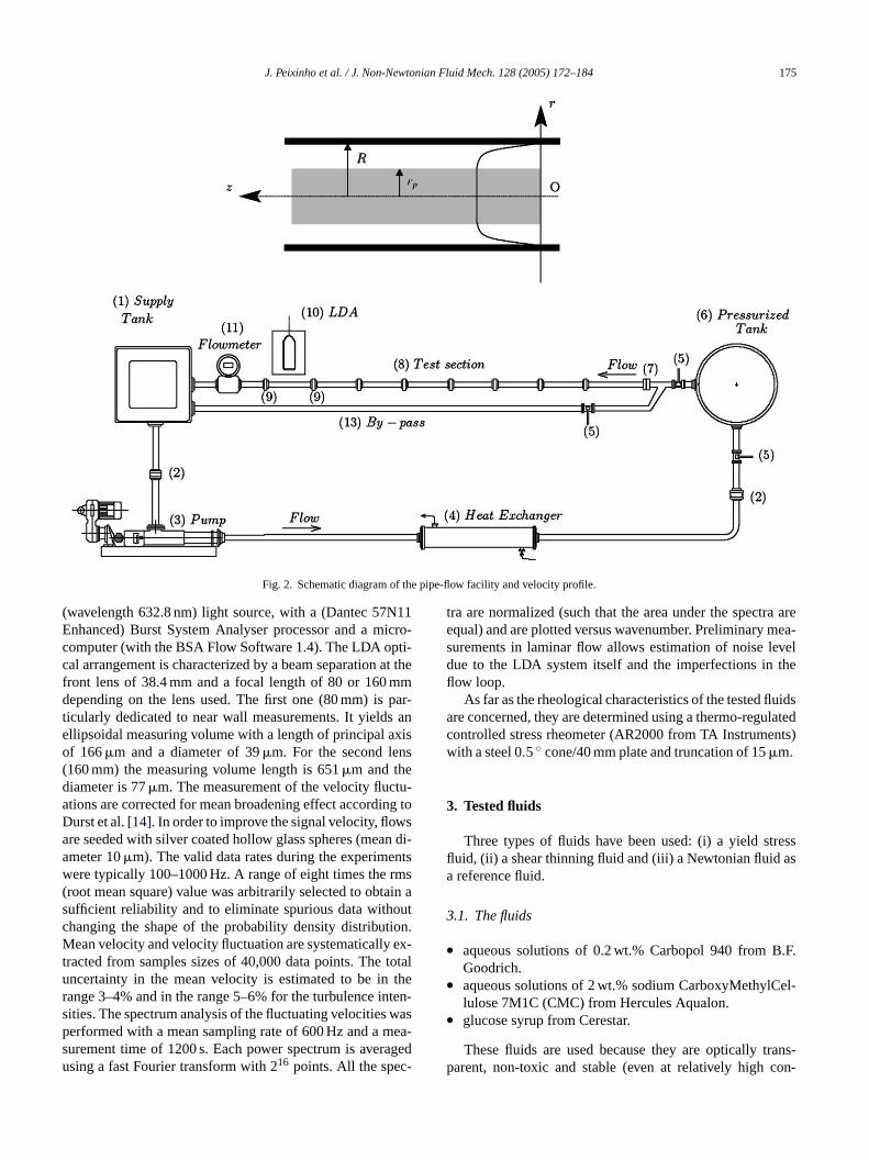
J. Peixinho et al. / J. Non-Newtonian Fluid Mech. 128 (2005) 172–184 175
Fig. 2. Schematic diagram of the pipe-flow facility and velocity profile.
(wavelength 632.8 nm) light source, with a (Dantec 57N11Enhanced) Burst System Analyser processor and a micro-computer (with the BSA Flow Software 1.4). The LDA opti-cal arrangement is characterized by a beam separation at thefront lens of 38.4 mm and a focal length of 80 or 160 mmdepending on the lens used. The first one (80 mm) is par-ticularly dedicated to near wall measurements. It yields anellipsoidal measuring volume with a length of principal axisof 166�m and a diameter of 39�m. For the second lens(160 mm) the measuring volume length is 651�m and thediameter is 77�m. The measurement of the velocity fluctu-ations are corrected for mean broadening effect according toDurst et al.[14]. In order to improve the signal velocity, flowsare seeded with silver coated hollow glass spheres (mean di-ameter 10�m). The valid data rates during the experimentswere typically 100–1000 Hz. A range of eight times the rms(root mean square) value was arbitrarily selected to obtain asufficient reliability and to eliminate spurious data withoutchanging the shape of the probability density distribution.Mean velocity and velocity fluctuation are systematically ex-tracted from samples sizes of 40,000 data points. The totaluncertainty in the mean velocity is estimated to be in therange 3–4% and in the range 5–6% for the turbulence inten-sities. The spectrum analysis of the fluctuating velocities wasperformed with a mean sampling rate of 600 Hz and a mea-surement time of 1200 s. Each power spectrum is averagedu -
tra are normalized (such that the area under the spectra areequal) and are plotted versus wavenumber. Preliminary mea-surements in laminar flow allows estimation of noise leveldue to the LDA system itself and the imperfections in theflow loop.
As far as the rheological characteristics of the tested fluidsare concerned, they are determined using a thermo-regulatedcontrolled stress rheometer (AR2000 from TA Instruments)with a steel 0.5◦ cone/40 mm plate and truncation of 15�m.
3. Tested fluids
Three types of fluids have been used: (i) a yield stressfluid, (ii) a shear thinning fluid and (iii) a Newtonian fluid asa reference fluid.
3.1. The fluids
• aqueous solutions of 0.2 wt.% Carbopol 940 from B.F.Goodrich.
• aqueous solutions of 2 wt.% sodium CarboxyMethylCel-lulose 7M1C (CMC) from Hercules Aqualon.
• glucose syrup from Cerestar.
These fluids are used because they are optically trans-p con-
sing a fast Fourier transform with 216 points. All the spec arent, non-toxic and stable (even at relatively high
176 J. Peixinho et al. / J. Non-Newtonian Fluid Mech. 128 (2005) 172–184
centrations), thereby facilitating LDA measurements. Aque-ous solutions of Carbopol and CMC are prepared by addingpowder into de-ionised water. Then, the Carbopol solutionis neutralized using sodium chloride. A gelification processaccompanies this neutralization. To prevent bacteriologicaldegradation of the fluids, a small amount of formaldehyde isadded.
3.2. Rheological properties
Fig. 3 shows the variation of shear viscosity vs. shearrate for the 0.2% Carbopol, the 2% CMC and the glucosesyrup. The rheograms are determined at the working tem-perature (20◦C). The experimental data for the 0.2% Car-bopol are fitted by the Herschel–Bulkley model accordingto Roberts and Barnes[15] and Kim et al.[16]. The rhe-ological tests were performed for a shear rate range simi-lar to that encountered in the pipe flow (0.1–4000 s−1). Onehas to note that the yield stressτY is no more than a fit-ting parameter, sensible to the resolution of the instrumen-tation at very low shear rates (some readers prefer the termapparent yield stress). For the 2% CMC solution, three re-gions can be distinguished depending on the shear rate: (i)a Newtonian region for low shear rate, (ii) a transition re-gion and (iii) a shear thinning region for high shear rate,which can be described by an Ostwald model. For the wholerr rossmt vis-c d byh gra-d og-i xperi-m th thec
s dif-f Ac-c al hes0f the2 bec ,r ievedb e.g.R
the2 andt uidsh firstn xhibits ina thee
Fig. 3. Shear stress vs. shear rate. The viscosity of the glucose syrup isµ =0.1 Pa s. The behaviour of the 2% CMC solution is described by the Crossmodel (µ0 = 0.46 Pa s,µ∞ = 13.6 mPa s,k = 4.75 ms,m = 0.71) and the0.2% Carbopol solution by the Herschel–Bulkley model (withτY = 7.2 Pa,K = 4.3 Pa sn andn = 0.47).
Fig. 4. First normal stress difference vs. shear stress. The lines are powerlaw models:N1 = 0.16τ1.4 and 0.08τ1.6, respectively for the 0.2% Carbopoland the 2% CMC solutions.
4. Results and discussion
The results are presented in three parts. The first one isdedicated to the laminar flow and the validation of our mea-surements. The second part is dedicated to the transitionalflow and the last one to the turbulent flow.
ange of shear rate, according to Escudier et al.[17], theheological behaviour can be well described by the Codel:µ = µ∞ + (µ0 − µ∞)[1 + (kγ)m]−1. On choosing
his fluid, we have in mind the regularized models ofoplastic fluids where the unsheared zone is replaceighly viscous Newtonian fluid. Due to the mechanical deation of the fluids particularly at high flow rate, the rheol
cal parameters are determined before and after each eental test, each reported experiment is associated wi
orresponding rheology.Fig. 4presents measurement of the first normal stres
erenceN1 as a function of the applied shear stress.ording to Barnes et al.[18] it can be considered thatiquid is elastic whenN1 in a shear flow is larger than thear stress. A power law fit toN1(τ) data leads toN1 =.163τ1.41 for the 2% CMC solution andN1 = 0.085τ1.63
or the 0.2% Carbopol solution. Using Barnes criteria% CMC solution and the 0.2% Carbopol solution canonsidered highly elastic fromτ > 90 Pa andτ > 110 Paespectively. These values of shear stress are not achefore reaching a fully developed turbulent flow (e′ > 4000).In summary, the flow curves of the 0.2% Carbopol and
% CMC are well described by the Herschel–Bulkleyhe Cross model, respectively. At high shear rate, both flave a similar shear thinning behaviour. According to theormal stress difference, both aqueous solutions also eimilar elastic properties. Consequently, during the flowpipe, the only difference between the two solutions is
xistence of a plug region.

J. Peixinho et al. / J. Non-Newtonian Fluid Mech. 128 (2005) 172–184 177
4.1. Laminar flow
According to Froishteter and Vinogradov[19], the en-trance length,Le, after which the laminar flow of a Herschel–Bulkley fluid is considered established is given by:
Le
RReg= 0.23
n0.31 − 0.4a (1)
wherea is the dimensionless radius of the plug zone,rp =aR and Reg is the Reynolds number defined by:Reg =ρU2−nRn/K. The Eq.(1) is used to ensure that our mea-surements concern a fully developed flow.
The Hagen–Poiseuille flow of a Herschel–Bulkley fluid ina cylindrical pipe of radiusR is described by:
0 = −dp
dz+ 1
r
d
dr(rτ) (2)
whereτ is given by:
τ = sgn(
dudr
)τY + K
∣∣∣dudr
∣∣∣n−1dudr |τ| ≥ τY
dudr = 0 |τ| ≤ τY
(3)
where, sgn (du/dr) is the sign of (du/dr), τY the yield stress,K the consistency, andn the flow behaviour index. Using theradiusRof the cylinder as length scale and the bulk velocity,U
≤ rR
< a
≤ rR
≤ 1(4)
w theyg∫
0
n’sm∞
w
Fig. 5. Dimensionless radius of the plug zone as a function of the Herschel–Bulkley number forn = 0.1,0.5 and 1.
Fig. 5showsaas a function ofHb for three values ofn: 1,0.5 and 0.1. The dashed lines show the asymptotic expansionsto a(Hb) valid for large and smallHb.
Fig. 6 is an example of measured velocity profiles forglucose syrup, 2% CMC solution and 0.2% Carbopol solution
in the laminar situation. For the yield stress fluid, the plugzone is delimited by vertical lines. For the correspondingrheology, Eq.(6) givesa = 0.17. For the shear thinning fluidthe velocity profile is determined numerically. Finally, theexperimental velocity profiles are in good agreement with thetheoretical ones (continuous, dashed and dotted lines) for thethree fluids. The maximum difference between measured andcalculated axial velocity does not exceed 2%. These resultsvalidate our velocity and rheological measurements.
In the following, the Reynolds number used is that definedby Metzner and Reed[2]. In the laminar regime, it satisfiesthe relationfRe′ = 16, weref is the Fanning friction factor.It can be shown that:
Re′ = ρU2−n′Dn′
8n′−1
k′ (8)
n
, as velocity scale, the dimensionless solution is:
u
U=
nn+1
(Hba
)1/n(1 − a)(n+1)/n 0
nn+1
(Hba
)1/n [(1 − a)(n+1)/n − (
rR
− a)(n+1)/n
]a
hereHb is the Herschel–Bulkley number (the ratio ofield stressτY to a nominal shear stressK(U/R)n). Using thelobal continuity equation:
1
0
u
U
r
Rd
( r
R
)= 1
2(5)
It can be shown that:
= (1 − a)(3n+1)/n − 3n + 1
n(1 − a)(2n+1)/n
+ (2n + 1)(3n + 1)
2n2 (1 − a)(n+1)/n
+ (3n + 1)(2n + 1)(n + 1)
2n3
( a
Hb
)1/n(6)
This equation is solved numerically using Newtoethod. The asymptotic behaviour ofa asHb → 0 orHb →are:
a ∼ (n
3+n
)nHb − 1
2n+1
(n
3+n
)2n−1Hb 2 as Hb → 0
a ∼ 1 − c1
(1Hb
)1/(1+n) + c2
(1Hb
)2/(1+n)as Hb → ∞
(7)
ith, c1 =(
1+nn
)n/(n+1)andc2 = 2n2
(2n+1)(n+1)c21
′ =
(1 − a) + 2a(1 − a)(1 + m)/(2 + m)
+(1 − a)2(1 + m)/(3 + m)
m + 1 − 3(1− a)[a2 + 2a(1 − a)(1 + m)/(2 + m)
+(1 − a)2(1 + m)/(3 + m)]
(9)

178 J. Peixinho et al. / J. Non-Newtonian Fluid Mech. 128 (2005) 172–184
Fig. 6. Laminar velocity profiles for a glucose syrup (µ = 0.1 Pa s,U =2.1 ms−1 andRe = 640), a 2% CMC (µ0 = 0.17 Pa s,µ∞ = 0.03 Pa s,k =2.24 ms,m = 0.96,U = 4.7 ms−1, andRe′ = 1200) and a 0.2% Carbopolsolution (τY = 46 Pa,K = 15 Pa s−n, n = 0.38, U = 3 ms−1, Hb = 0.42andRe′ = 280).
k′ =(Km
4
)n′ (τY
a
)1−n′m{
(1 − a)1+m
×[1 + 2(1− a)(1 + m)
a(2 + m)+ (1 − a)2(m + 1)
a2(3 + m)
]}−n′
(10)
wherem = 1/n. Expressions forn′ and k′ depend on theHerschel–Bulkley model parameters and the radius of theplug a (obtained by resolving Eq.(6)). Koziki et al. [20]determinedn′ andk′ for several rheological models and ductsarbitrary cross section.
The friction factorf is: f = 2τwρU2 with τw = R
2!pLp
, whereρ is the density and!p a pressure drop over the lengthLpbetween the two pressure tappings along the pipe. The evolu-tion of the friction factorf as a function ofRe′ is presented inFig. 7. In the laminar flow situation (e.g.Re′ < 2000), goodagreement is observed between the experimental measure-ments and the generalized Hagen–Poiseuille law (fRe′ = 16)for the three fluids used.
Fig. 8shows the dimensionless centreline velocityuc/U
versusRe′, the continuous, dashed and dotted lines representthe theoretical solutions. The ratiouc/U increases withRe′for the 0.2% Carbopol solution (the plug core dimension de-c .O d andc ea-s tup.
Fig. 7. Friction factorf vs. Reynolds numberRe′. The viscosity of theglucose syrup isµ = 50 mPa s. The behaviour of the 2% CMC solu-tion is described by the Cross model (µ0 = 67.1 mPa s,µ∞ = 4.28 mPa s,k = 1.12 ms,m = 0.68) and the 0.2% Carbopol solution by the Herschel–Bulkley model (withτY = 6.3 Pa,K = 2.2 Pa sn andn = 0.5).
4.2. Transitional flow
Fig. 9 illustrates the flow evolution from laminar (a) toturbulent (e) regime for the 0.2% Carbopol solution. With in-
F eg tioni1 kleym
reases) and it decreases withRe′ for the 2% CMC solutionnce again the maximum difference between measurealculated axial velocity does not exceed 2%. All the murements for laminar flow validate our experimental se
ig. 8. Normalized centerline velocityuc/U vs.Re′. The viscosity of thlucose syrup isµ = 50 mPa s. The behaviour of the 2% CMC solu
s described by the Cross model (µ0 = 67.1 mPa s,µ∞ = 4.28 mPa s,k =.12 ms,m = 0.68) and the 0.2% Carbopol solution by the Herschel–Bulodel (withτY = 2.3 Pa,K = 1.9 Pa sn andn = 0.5).

J. Peixinho et al. / J. Non-Newtonian Fluid Mech. 128 (2005) 172–184 179
Fig. 9. Mean velocity profiles for increasing Reynolds numbers of 0.2% Car-bopol (τy = 8 Pa,K = 2.6 Pa s−n, n = 0.49 andHb = 0.182,0.088,0.08and 0.073, respectively forRe′ = 500,1650,1800 and 3300).
creasing the Reynolds number, the experimental velocity pro-files (c–d) depart from the corresponding theoretical laminarones represented by lines. The experimental velocity profilein the transitional regime present an unexpected asymmetry.This repeatable asymmetry also has been observed by Escud-ier and Presti[13]. It is the object of ongoing investigations.
To determine the critical Reynolds number, the measuredcentreline velocity is represented as a function ofRe′ (Fig.8). At the critical condition, the experimental values startto depart from the theoretical laminar solutions given in theprevious section. The same method is used with the friction
Fig. 10. Relative velocity fluctuations vs. Metzner and Reed Reynolds num-ber. The viscosity of the glucose syrup isµ = 50 mPa s. The behaviour ofthe 2% CMC solution is described by the Cross model (µ0 = 67.1 mPa s,µ∞ = 4.28 mPa s,k = 1.12 ms,m = 0.68) and the 0.2% Carbopol solu-tion by the Herschel–Bulkley model (withτY = 2.3 Pa,K = 1.9 Pa sn andn = 0.5).
factorf (Re′) (Fig. 7) as well as the centreline velocity fluc-
tuations√
u′2c /uc(Re′) (Fig. 10). One can note that the mean
centreline velocity and the centreline velocity fluctuations areextracted from the same velocity signal. The results are sum-marized inTable 1. The critical conditions calculated fromthree different phenomenological criteria are also given forcomparison. Mishra and Hanks criteria are the most in agree-ment with the experimental results. It is clear that the shearthinning and the yield stress delay the transition as observedby Pinho and Whitelaw[21], Park et al.[12] and Escudier andPresti[13]. The results given inTable 1also show that for flu-ids without yield stress (i.e. glucose and CMC solutions), the
critical Reynolds number evaluated using√
u′2c /uc(Re′) is
lower than that obtained fromuc/U(Re′) orf (Re′) measure-
ments. The method based on the analysis of the√
u′2c /uc(Re′)
is more sensitive to detect the beginning of the transitionthan the other two methods. However, for the 0.2% Carbopol
Table 1Phenomenological and experimental criteria : the glucose syrup is a Newtonian fluid (with a viscosity of 50 mPa s)
Fluids Experimental criteria Phenomenological criteria
f (Re′) ucU
(Re′)
√u′2
cuc
(Re′) Mishra Hanks Slatter
Glucose syrup 2100 2050 1800 2100 2100 21002% CMC 2500 2300 21000.2% Carbopol 2700 2550 3300
The behaviour of the 2% CMC solution is described by the Cross model (µ0 =Carbopol solution by the Herschel–Bulkley model (withτY = 2.3 Pa,K = 1.9 Pa
2230 2268 –2485 2380 1907
67.1 mPa s,µ∞ = 4.28 mPa s,k = 1.12 ms andm = 0.68) and the 0.2%sn andn = 0.5).
180 J. Peixinho et al. / J. Non-Newtonian Fluid Mech. 128 (2005) 172–184
solution,Re′c from
√u′2
c /uc(Re′) is larger thanRe′c from
uc/U(Re′) or f (Re′). This case will be analyzed in detaillater.
Concerning the transition,Fig. 8 shows the evolution ofuc/U(Re′) for the fluids used. Different stages can be dis-tinguished. For the Newtonian fluid, an abrupt decrease ofthe ratiouc/U is observed for 2000< Re < 3000. Then, forRe > 3000, the ratio is close to values given in the literatureby Pinho and Whitelaw[21]. For the 2% CMC solution, theevolution is similar to that for a Newtonian fluid. In the caseof the Herschel–Bulkley fluid, the evolution ofuc/U versusRe′ can be described in three stages. In the first stage,uc/U
(instead of increasing goes in the opposite direction and) de-creases slightly with increasingRe′. In the second stage, anabrupt decrease ofuc/U is observed and in the third stage(Re′ > 4000), the decrease ofuc/U becomes weaker. Thevertical lines representRe′ = 2550 andRe′ = 3300.
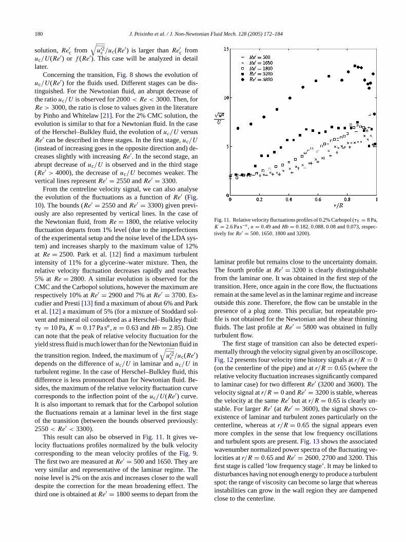
From the centreline velocity signal, we can also analysethe evolution of the fluctuations as a function ofRe′ (Fig.10). The bounds (Re′ = 2550 andRe′ = 3300) given previ-ously are also represented by vertical lines. In the case ofthe Newtonian fluid, fromRe = 1800, the relative velocityfluctuation departs from 1% level (due to the imperfectionsof the experimental setup and the noise level of the LDA sys-tem) and increases sharply to the maximum value of 12%at Re = 2500. Park et al.[12] find a maximum turbulenti ther ches5 heC arer -c rke ol-v uid:τ
c they d in
tdt thisd Be-s rvecI tiont tageo usly:2
l itycT rev Then walld Thet he
Fig. 11. Relative velocity fluctuations profiles of 0.2% Carbopol (τY = 8 Pa,K = 2.6 Pa s−n, n = 0.49 andHb = 0.182,0.088,0.08 and 0.073, respec-tively for Re′ = 500,1650,1800 and 3200).
laminar profile but remains close to the uncertainty domain.The fourth profile atRe′ = 3200 is clearly distinguishablefrom the laminar one. It was obtained in the first step of thetransition. Here, once again in the core flow, the fluctuationsremain at the same level as in the laminar regime and increaseoutside this zone. Therefore, the flow can be unstable in thepresence of a plug zone. This peculiar, but repeatable pro-file is not obtained for the Newtonian and the shear thinningfluids. The last profile atRe′ = 5800 was obtained in fullyturbulent flow.
The first stage of transition can also be detected experi-mentally through the velocity signal given by an oscilloscope.Fig. 12presents four velocity time history signals atr/R = 0(on the centerline of the pipe) and atr/R = 0.65 (where therelative velocity fluctuation increases significantly comparedto laminar case) for two differentRe′ (3200 and 3600). Thevelocity signal atr/R = 0 andRe′ = 3200 is stable, whereasthe velocity at the sameRe′ but atr/R = 0.65 is clearly un-stable. For largerRe′ (atRe′ = 3600), the signal shows co-existence of laminar and turbulent zones particularly on thecenterline, whereas atr/R = 0.65 the signal appears evenmore complex in the sense that low frequency oscillationsand turbulent spots are present.Fig. 13shows the associatedwavenumber normalized power spectra of the fluctuating ve-locities atr/R = 0.65 andRe′ = 2600,2700 and 3200. Thisfirst stage is called ‘low frequency stage’. It may be linked tod ulents ereasi nedc
ntensity of 11% for a glycerine–water mixture. Then,elative velocity fluctuation decreases rapidly and rea% atRe = 2800. A similar evolution is observed for tMC and the Carbopol solutions, however the maximum
espectively 10% atRe′ = 2900 and 7% atRe′ = 3700. Esudier and Presti[13] find a maximum of about 6% and Pat al.[12] a maximum of 5% (for a mixture of Stoddard sent and mineral oil considered as a Herschel–Bulkley flY = 10 Pa,K = 0.17 Pa sn, n = 0.63 andHb = 2.85). Onean note that the peak of relative velocity fluctuation forield stress fluid is much lower than for the Newtonian flui
he transition region. Indeed, the maximum of√
u′2c /uc(Re′)
epends on the difference ofuc/U in laminar anduc/U inurbulent regime. In the case of Herschel–Bulkley fluid,ifference is less pronounced than for Newtonian fluid.ides, the maximum of the relative velocity fluctuation cuorresponds to the inflection point of theuc/U(Re′) curve.t is also important to remark that for the Carbopol soluhe fluctuations remain at a laminar level in the first sf the transition (between the bounds observed previo550< Re′ < 3300).
This result can also be observed inFig. 11. It gives ve-ocity fluctuations profiles normalized by the bulk velocorresponding to the mean velocity profiles of theFig. 9.he first two are measured atRe′ = 500 and 1650. They aery similar and representative of the laminar regime.oise level is 2% on the axis and increases closer to theespite the correction for the mean broadening effect.
hird one is obtained atRe′ = 1800 seems to depart from t
isturbances having not enough energy to produce a turbpot: the range of viscosity can become so large that whnstabilities can grow in the wall region they are dampelose to the centerline.

J. Peixinho et al. / J. Non-Newtonian Fluid Mech. 128 (2005) 172–184 181
Fig. 12. Velocity time history for a 0.2% Carbopol solution (τY = 2.3 Pa,K = 10 Pa s−n, andn = 0.32) (a) r/R = 0 andRe′ = 3200, (b) r/R = 0.65 andRe′ = 3200, (c) r/R = 0 andRe′ = 3600 and (d) r/R = 0.65 andRe′ = 3600.
During the first stage of the transition, the centreline ve-locity signal remains similar to that in the laminar regime. Inthe second stage of the transition, turbulent spots are observedexperimentally.Fig. 12(c)is a sample of velocity time his-tory atRe′ = 3600 on the centerline of the pipe. From this, anisolated turbulent spot in dimensionless form is given byFig.14(a). Inside the spot, the plug zone is disrupted due to largevelocity variations. In the laminar phase between two spots,the presence of the plug zone is possible. Hence, if the lengthof the pipe is sufficiently long, a discontinuous plug zone canbe observed.Fig. 14shows typical spots for the CMC solu-tion (Fig. 14(b)), glucose syrup (Fig. 14(c)) and that given byDarbyshire and Mullin[22] for water (Fig. 14(d)). It can beobserved that all the spots have practically the same length
Fig. 13. Normalized power spectra of axial velocity fluctuation of a 0.2%Carbopol solution (τY = 2.3 Pa,K = 10 Pa s−n, andn = 0.32) at the posi-tion r/R = 0.65 during the first stage of transition atRe′ = 2600, 2700 and3200.
scale (� 25D). The velocity variation between the laminarand turbulent phase depends on the non-Newtonian charac-ter of the fluid as explained before. With increasingRe′, thecontinuous development of several turbulent spots leads tocompletely turbulent flow.
4.3. Turbulent flow
The analysis of the turbulent flow at low Reynolds numberfor the three fluids considered is made through friction factormeasurements as a function of the wall Reynolds numberRew (based on the wall viscosity). The mean velocity profileand the turbulent intensity profile of the axial velocity arealso considered.
4.3.1. Friction factorThe variation of friction factor withRew is presented in
Fig. 15. The experimental measurements for glucose syrupare in very good agreement with Blasius law forRe > 3000.For Carbopol solution, the experimental results are lowerthan the Dodge and Metzner correlation[23] (representedas dashed lines). Actually, at theseRew, the elasticity of thefluid leads to the drag reduction effect such that the drag re-duction coefficient (DR = 100(f − fN)/fN wherefN is thefriction factor for a Newtonian fluid) is about 30 and 35% int pols
4e
o p,y
0 mal-if re-l ela sa showd in-
he range ofRew tested, respectively for the 0.2% Carboolution and the 2% CMC solution.
.3.2. Mean velocity profileVelocity profiles are presented inFig. 16. The centrelin
f the pipe corresponds toy+c ≈ 144 for the glucose syru
+c ≈ 270 for the 2% CMC solution andy+
c ≈ 283 for the.2% Carbopol solution. For the glucose syrup, the nor
zed velocity profile agrees with the linear relation:u+ = y+or 0 < y+ < 5 and the low Reynolds number logarithmication: u+ = 2.5 lny+ + 5.5 for y+ > 30 obtained by Patnd Head[24]. Dodge and Metzner[2] and Virk correlationre represented by dashed lines. Velocity measurementsrag reduction effects. It is difficult to conclude upon the

182 J. Peixinho et al. / J. Non-Newtonian Fluid Mech. 128 (2005) 172–184
Fig. 14. Time trace of the axial velocity on the centerline of the pipe (a) for a 0.2% Carbopol solution (τY = 2.3 Pa,K = 10 Pa s−n, n = 0.32, andRe′ = 3600),(b) for a 2% CMC solution (µ0 = 67.1 mPa s,µ∞ = 4.28 mPa s,k = 1.12 ms,m = 0.68, andRe′ = 3280) , (c) for a glucose syrup (µ = 105 Pa s,Re = 2000),and (d) from Darbyshire and Mullin[22] for water (atRe � 2200).
fluence of the shear thinning since the elasticity of the fluidsis important. Indeed, from pressure measurements (Fig. 15)and first normal stress measurement (Fig. 4), one can estimatethe first normal stress is higher than the wall shear stress nearthe wall.
Fig. 15. Friction factorf vs. Reynolds numberRe′. The viscosity of theglucose syrup isµ = 50 mPa s. The behaviour of the 2% CMC solutionis described by the Cross model (µ0 = 67.1 mPa s,µ∞ = 4.28 mPa s,k =1.12 ms andm = 0.68) and the 0.2% Carbopol solution by the Herschel–Bulkley model (withτY = 6.3 Pa,K = 2.2 Pa sn andn = 0.5).
4.3.3. Turbulent intensity profile
Fig. 17 represents√
u′2/uτ as a function ofy+. It in-creases from the wall and reaches a maximum before de-creasing. For the glucose syrup, the experimental results are
Fig. 16. Mean velocity profile. The viscosity of the glucose syrup isµ = 52 mPa s andRe = 4000. The behaviour of the 2% CMC solutionis described by the Cross model (µ0 = 67.1 mPa s,µ∞ = 4.28 mPa s,k =1.12 ms andm = 0.68) andRew = 12000. The 0.2% Carbopol solution isdescribed by the Herschel–Bulkley model (withτY = 5.5 Pa,K = 3 Pa s−n
andn = 0.49) andRew = 10000.

J. Peixinho et al. / J. Non-Newtonian Fluid Mech. 128 (2005) 172–184 183
Fig. 17. Turbulent intensity profile. The viscosity of the glucose syrup isµ = 52 mPa s andRe = 4000. The behaviour of the 2% CMC solution isdescribed by the Cross model (µ0 = 67.1 mPa s,µ∞ = 4.28 mPa s,k =1.12 ms andm = 0.68) andRew = 12000. The 0.2% Carbopol solution isdescribed by the Herschel–Bulkley model (withτY = 5.5 Pa,K = 3 Pa s−n
andn = 0.49) andRew = 10000.
in a very good agreement with those given by Durst et al.[14], the peak of the turbulence intensity is 2.6 and located aty+ � 12. For the 2% CMC solution and the 0.2% Carbopolsolution, the peak is higher than for Newtonian fluid. Themeasurements of axial velocity for Carbopol and CMC solu-tions are difficult fory+ < 10 (actuallyy+ = 10 correspondto y ≈ 0.2 mm). This is why there is a lack of experimentaldata inFig. 17for low y+. Once again there is a dominanteffect of the elasticity of the fluids. Nevertheless, our mea-surement shows the peak of the axial turbulence intensity islarger than for Newtonian fluids.
5. Conclusion
In this paper, detailed measurements have been carriedout in laminar, transitional and turbulent pipe flow of a yieldstress fluid (0.2% Carbopol solution), a shear thinning fluid(2% CMC solution) and a Newtonian fluid (glucose syrup).The first normal stress differences are similar for the twonon-Newtonian fluids. In laminar flow, the experimental ve-locity profiles and the friction factor are well described bythe theoretical solution. The critical conditions from whichthe centreline velocity and the pressure drop measurementsdepart from theoretical solutions are determined. The resultss s in-c arec emst
and Mishra et al.[6] are the most appropriate to predict ourresults.
The transition for the yield stress fluid takes place in twostages. First, the experimental velocity profile departs slightlyfrom the laminar theoretical solution, however, the fluctua-tions remain at a laminar level in a zone flow around the axisand increase slightly outside this zone. In the annular zone,low frequency oscillations of the axial velocity are observed.Then, with increasing the Reynolds number, turbulent spotsfilling up the whole section appear. Inside the spot, the plugzone is disrupted due to large velocity variations. Betweentwo successive spots, the flow is laminar, then the presenceof the plug zone is possible.
In turbulent flow, the friction factor measurements andvelocity profiles show the drag reduction effect for both the2% CMC and the 0.2% Carbopol solutions. Near the axis,the longitudinal turbulence intensities are similar to that ofNewtonian fluid. However, in the vicinity of the wall, the axialrelative turbulence intensities are larger than for Newtonianfluid. This is in agreement with Park et al.[12].
Acknowledgments
The authors would like to thank our colleagues for usefuld ncials kharf
R
[ ids,
[ n of33–
[ ield
[ em.
[ in
[ ely915–
[ on-e on, pp.
[ ng-gical
[ ing-
[ entluid
[ pipe13.
how that both the shear thinning and the yield stresreases the stability of the flow. The critical conditionsompared with various phenomenological criteria. It sehat the global stability criterion given by Hanks et al.[3]
iscussion, the management of Schlumberger for finaupport and permission to publish this work and M. Belaor her assistance in some of the latest experiments.
eferences
1] R.B. Bird, G.C. Armstrong, O. Hassager, Dynamics of Polymer Liquvol. 1, Wiley, 1977.
2] A.B. Metzner, J.C. Reed, Flow of non-Newtonian fluids-correlatiolaminar, transition and turbulent-flow regions, A.I.Ch.E. J. 1 (1955) 4435.
3] R.W. Hanks, The laminar-turbulent transition for fluids with a ystress, A.I.Ch.E. J. 9 (1963) 306–309.
4] B.O.A. Hedstrom, Flow of plastics materials in pipes, Ind. Eng. Ch44 (3) (1952) 651–656.
5] N.W. Ryan, M.M. Johnson, Transition from laminar to turbulent flowpipes, A.I.Ch.E. J. 5 (1959) 433–435.
6] P. Mishra, G. Tripathi, Transition from laminar to turbulent flow of purviscous non-Newtonian fluids in tubes, Chem. Eng. Sci. 26 (1971)921.
7] P.T. Slatter, The laminar-turbulent transition prediction for nNewtonian slurries, Proceedings of the International ConferencProblems in Fluid Mechanics and Hydrology, vol. 1, Prague, 1999247–256.
8] C. Nouar, I.A. Frigaard, Non-linear stability of Poiseuille flow of a Biham fluid: theoretical results and comparison with phenomenolocriteria, J. Non-Newtonian Fluid Mech. 100 (2001) 127–149.
9] I.A. Frigaard, S.D. Howison, I.J. Sobey, On the stability flow of a Bham fluid, J. Fluid Mech. 263 (1994) 133–150.
10] A.A. Draad, G.D.C. Kuiken, F.T.M. Nieuwstadt, Laminar-turbultransition in pipe flow for Newtonian and non-Newtonian fluids, J. FMech. 377 (1996) 267–312.
11] M.P. Escudier, F. Presti, S. Smith, Drag reduction in the turbulentflow of polymers, J. Non-Newtonian Fluid Mech. 81 (1999) 197–2
184 J. Peixinho et al. / J. Non-Newtonian Fluid Mech. 128 (2005) 172–184
[12] J.T. Park, R.J. Mannheimer, T.A. Grimley, T.B. Morrow, Pipe flowmeasurement of a transparent non-Newtonian slurry, J. Fluids Eng. 111(1989) 331–336.
[13] M.P. Escudier, F. Presti, Pipe flow of a thixotropic liquid, J. Non-Newtonian Fluid Mech. 62 (1996) 291–306.
[14] F. Durst, J. Jovanovic, J. Sender, LDA measurements in the near-wallregion of a turbulent pipe flow, J. Fluid Mech. 295 (1995) 305–335.
[15] G.P. Roberts, H.A. Barnes, New measurements of the flow-curves forCarbopol dispersions without slip artefacts, Rheol. Acta 40 (2001) 499–503.
[16] J.-Y. Kim, J.-Y. Song, E.-J. Lee, S.-K. Park, Rheological propertiesand microstructures of Carbopol gel network system, Colloid Polym.Sci. 281 (2003) 614–623.
[17] M.P. Escudier, I.W. Gouldson, A.S. Pereira, F.T. Pinho, R.J. Poole, Onthe reproducibility of the rheology of shear-thinning liquids, J. Non-Newtonian Fluid Mech. 97 (2001) 99–124.
[18] H.A. Barnes, J.F. Hutton, K. Walters, An introduction to Rheology,Elsevier, 1989.
[19] G.B. Froishteter, G.V. Vinogradov, The laminar flow of plastic dispersesystems in circular tubes, Rheol. Acta 19 (1980) 239–250.
[20] W. Kozicki, C.H. Chou, C. Tiu, Non-Newtonian flow in ductsof arbitrary cross-section shape, Chem. Eng. Sci. 21 (1966) 665–679.
[21] F.T. Pinho, J.H. Whitelaw, Flow of non-Newtonian fluids in a pipe, J.Non-Newtonian Fluid Mech. 34 (1990) 129–144.
[22] A.G. Darbyshire, T. Mullin, Transition to turbulence in constant-mass-flux pipe flow, J. Fluid Mech. 289 (1995) 83–114.
[23] D.W. Dodge, A.B. Metzner, Turbulent flow of non-Newtonian systems,A.I.Ch.E. J. 5 (1959) 189–204.
[24] V.C. Patel, M.R. Head, Some observations on skin friction and velocityprofiles in fully developed pipe and channel flows, J. Fluid Mech. 38(1969) 181–201.


![Laminar-Turbulent Patterning in Transitional Flows · boundary effects enforce the spatial coherence of nonlinear modes (see §3.3.2–4 in [2]). Confinement effects are appreciated](https://static.fdocuments.net/doc/165x107/5f35854a79c86d19be0ccdf8/laminar-turbulent-patterning-in-transitional-flows-boundary-effects-enforce-the.jpg)


