Lalit Sivanandan Nookala - University of Minnesota Duluth
63
Weather Impact on Traffic Conditions and Travel Time Prediction by Lalit Sivanandan Nookala October 2006 Submitted in partial fulfillment of the Requirements for the degree of Master of Science Under the instruction of Dr. Donald Crouch Department of Computer Science University of Minnesota Duluth Duluth, Minnesota 55812 U. S. A.
Transcript of Lalit Sivanandan Nookala - University of Minnesota Duluth
Weather Impact on Traffic Conditions and Travel Time Prediction
by
Lalit Sivanandan Nookala
October 2006
Submitted in partial fulfillment of the
Requirements for the degree of
Master of Science
Under the instruction of Dr. Donald Crouch
Department of Computer Science
University of Minnesota Duluth
Duluth, Minnesota 55812
U. S. A.

UNIVERSITY OF MINNESOTA DULUTH
This is to certify that I have examined this copy of master’s thesis by
Lalit Sivanandan Nookala
And have found that it is completed and satisfactory in all aspects,
and that any and all revisions required by the final examining committee have been made.
Dr. Donald Crouch
_______________________________
Name of Faculty Advisor
______________________________
Signature of Faculty Advisor
_____________________________
Date
GRADUATE SCHOOL

i
ABSTRACT
Traffic congestion is caused by various factors such as accidents, inclement
weather conditions, road maintenance work etc. In this work, the traffic congestion
caused by weather conditions is studied and the effect of weather conditions on traffic
volume and travel time is analyzed. The weather conditions are recorded by the RWIS
sites for various locations in and around twin cities metro area. The values recorded using
RWIS gives more localized weather conditions and hence is useful in assessing the effect
on traffic. Color-coded daily traffic volume graph with the corresponding color-coded
volume/occupancy graph are analyzed to study the effect of weather conditions on traffic.
It has been observed that the traffic congestion increases due to inclement weather
conditions because the freeway capacity drops and the traffic demand does not drop
accordingly. It has also been observed that during severe snow conditions the traffic
demand also drops significantly and the congestion on the freeway disappears. Further,
the short term travel time prediction using time-varying coefficients was done for the
days that had been affected by severe weather conditions. The error in the prediction was
high due to congestion caused by the weather conditions and a part of this work was
devoted to reduce this error. It had been observed that the error in prediction is related to
the change in the traffic occupancy of the road. A new prediction model that is an
extension of the time-varying prediction model has been proposed as the part of this
thesis that incorporates the change of occupancy caused due to weather conditions. It has
been observed that the prediction error reduces with the new model.

ii
ACKNOWLEDGEMENTS
I am grateful to my thesis advisor Dr. Taek Kwon for giving me an opportunity to
work under him and for guiding me. I wish to thank him for boosting my confidence with
his constant encouragement. Without his support and contribution, this thesis would not
have been possible.
I would like to thank my thesis committee members Dr. Donald Crouch and Dr.
Gary Shute for their interest in my thesis and their helpful suggestions. I am grateful to
Carol Wolosz from the NATSRL office for her help and to Linda Meek, Lori Lucia, Jim
Luttinen and the faculty at Computer Science Department at UMD for their support. Last
but not the least, I take this opportunity to thank my family and my friends.

iii
TABLE OF CONTENTS
LIST OF FIGURES ...................................................................................................................... v
LIST OF TABLES ....................................................................................................................... vi
CHAPTER 1 : INTRODUCTION............................................................................................... 1
1.1 Traffic Congestion Issues ............................................................................................... 1
1.2 Related Work on Travel Time Prediction....................................................................... 2
1.3 Road Weather Information System (RWIS) (Kwon, Fleege 2000)................................ 3
1.4 Objective of thesis........................................................................................................... 4
CHAPTER 2 : THEORETICAL BACKGROUND................................................................... 6
2.1 Traffic Parameters ................................................................................................................. 6
2.1.1 Traffic Volume .....................................................................................................6
2.1.2 Traffic Flow Rate .................................................................................................6
2.1.3 Occupancy.........................................................................................................7
2.1.4 Traffic Density ......................................................................................................7
2.1.5 Traffic Speed .......................................................................................................7
2.1.6 Travel Time ...........................................................................................................8
2.1.7 Traffic Capacity ..................................................................................................8
2.1.8 Traffic Demand ...................................................................................................9
2.2 Prediction of Travel Time ................................................................................................... 10
2.2.1 Time-varying coefficients for short-term travel time prediction (Zhang, Rice 2001)....................................................................................................................10
2.2.2 Day to day travel time trends and travel time prediction from the loop detector data (Kwon, Coifman, Bickel 2000) .......................................................12
CHAPTER 3 : DATA SOURCE AND METHODOLOGY.................................................... 14
3.1 Site Selection and Data Source ........................................................................................... 14

iv
3.2 Relational Database............................................................................................................. 15
3.3 Methodologies Used to Analyze Weather Impact on Traffic ............................................. 16
3.3.1 Correlation coefficients...................................................................................16
3.3.2 Effect of pavement conditions on daily total volume...............................17
3.3.3 Effect of pavement conditions on traffic dynamics ..................................17
3.4 Methodology to analyze weather impact on travel time prediction .................................... 20
3.4.1 Travel time estimation......................................................................................20
3.4.2 Time-varying coefficients for travel time prediction ..................................20
CHAPTER 4 : EXPERIMENTAL RESULTS......................................................................... 24
4.1 Correlation Coefficient Matrix............................................................................................ 24
4.2 Impact of Pavement Conditions on Daily Traffic Volume ................................................. 26
4.3 Impact of Pavement Conditions on Congestion.................................................................. 30
4.3.1 Case 1: Increased congestion by snow .......................................................30
4.3.2 Case2: Reduction of congestion by a severe snow event.......................32
4.3.3 Case 3: Increased congestion by damp conditions .................................33
4.3.4 Case4: Volume decrease and increase of congestion by wet conditions....................................................................................................................34
4.3.5 Case 5: Changes in pavement conditions ..................................................37
4.4 Impact of inclement weather conditions on travel time prediction..................................... 39
4.4.1 Case1: Effect of travel time prediction when weather conditions do not cause congestion......................................................................................................39
4.4.2 Case 2: Effect of travel time prediction by before-and-after weather events ..........................................................................................................................41
4.4.3 Case3: Wet and damp pavement conditions in the morning peak time......................................................................................................................................43
4.4.4 Case 4: The whole day is affected by snow................................................45
4.4.5 Case 5: Multiple changes of weather changes during the day..............47

v
CHAPTER 5 : CONCLUSION.................................................................................................. 50
5.1 Conclusion........................................................................................................................... 50
5.2 Future Recommendations.................................................................................................... 51
REFERENCES............................................................................................................................ 53
LIST OF FIGURES
Figure 3.1: Location of R/WIS sites in and around the metro area used for the study......14
Figure 4.1: Effect of pavement conditions on the traffic volume of Little Canada on January 4th and January 11th in 2005. The volume/occupancy graphs of the corresponding days are also presented.......................................................................................................31
Figure 4.2: Effect of severe snow conditions on the traffic volume. The volume/occupancy graphs of the corresponding days are also presented..........................33
Figure 4.3: Effect of damp pavement conditions on the traffic volume. ...........................34
Figure 4.4: Effect of wet pavement conditions on the traffic volume. The volume/occupancy graphs of the corresponding days are also presented..........................36
Figure 4.5: Effect of different pavement conditions on the traffic volume. The volume/occupancy graphs of the corresponding days are also presented..........................38
Figure 4.6: Travel time is affected by the snow conditions and is adjusted but the severe snow condition reduces the total traffic volume and the congestion disappears and the travel time prediction error between the baseline estimate and the prediction model is very low. ............................................................................................................................41
Figure 4.7: Travel time is affected by the snow conditions and is adjusted by the formula given in the equation. The change in the weather condition though reduces the traffic volume but also increases the congestion which increases the travel time. The PPE graphs shows the error that occurs due to the change in weather..................................................42
Figure 4.8: Travel time is affected by the damp conditions and is adjusted. The damp conditions increases congestion and travel time that is underestimated by the prediction model..................................................................................................................................44

vi
Figure 4.9: Travel time is affected by the snow conditions and the weather condition does not change. The snow conditions increases the travel time and the prediction model is erroneous due to the weather condition. ............................................................................46
Figure 4.10: Travel time prediction is severely affected by changing weather conditions and the prediction model is unable to predict the travel time accurately. The TVWI equation computes the travel time and the error in prediction are reduced. ......................48
LIST OF TABLES
Table 2.1: Length Based Classification Boundaries ............................................................8
Table 3.1: R/WIS sites and detectors in the proximity .....................................................15
Table 4.1: The correlation coefficient matrix for January 2005 at the Little Canada site .25
Table 4.2: The correlation coefficient matrix for June 2005 at the Little Canada site ......26
Table 4.3: Surface Conditions in Number of Hours and Traffic Volume at the Little Canada Site in January 2005..............................................................................................28

1
CHAPTER 1 : INTRODUCTION
1.1 Traffic Congestion Issues
As the number of vehicles on the road steadily increases and the expansion of
roadways is remained static, congestion on urban freeways became one of the major
transportation issues in US. Urban traffic costs 3.7 billion hours of travel delay and $63
billion per annum in the USA (Shrank, Lomax, 2005). Two ways can be considered to
reduce congestion on urban freeways; one is to increase the total freeway capacity by
expanding the number of lanes on the existing roads or new roads, but this requires extra
lands and enormous expenditure on the infrastructure which is often not viable in many
urban areas. Another solution is to use various traffic control strategies in order to
efficiently use the existing freeways. The control strategies often involve predicting
congestion levels and proactively managing the traffic before congestion is reached.
Among many parameters, travel time is one of the indicators that helps in determining the
future states of the freeway sections (Ben-Avika et al, 1992)
Congestion can happen due to various conditions such as road work, peak hour
traffic, accidents, and inclement weather conditions (Chin et al 2004). The primary
objective of this thesis is to analyze the effect of inclement weather conditions on traffic.
It is known that inclement weather conditions decrease traffic demand while they also
decrease the freeway capacity (Goodwin, 2002). If the decrease rate of the freeway
capacity is faster than the decrease of the traffic demand, traffic congestion is bound to
occur. It has been noted that 15% of the congestion occur due to bad weather conditions
(Cambridge Systematics, 2005). However, it is still unclear on how much traffic
demand and freeway capacity decreases occur under adverse weather conditions. It is
also unknown what level of the demand/capacity imbalance causes the congestion and
how much the travel time is affected. This thesis will attempt to answer some of these
questions by analyzing the Twin Cities’ freeway and Road Weather Information System
(RWIS) data.

2
1.2 Related Work on Travel Time Prediction
Predicting travel time is difficult for various reasons. To predict travel time for a
section of a road, traffic conditions or the speed changes of the vehicles along the section
must be estimated. It is difficult to accurately estimate the traffic conditions since they
can widely vary in spatial and time domain (Hall, Persaud 1989).
In order to predict travel time, past history of travel time is one of the most
important measures. Several ways of collecting travel time data exist. The Automated
Vehicle Identification (AVI) is a recent technology that is being used to measuring travel
time (Dion, Rakha, TRB 2003). The AVI system has various AVI tags and AVI reader
system and a computer system to store the data that is required for processing. The AVI
data processing system computes the travel time. Several research programs presently try
to utilize cell phones in the vehicles for measuring the travel time (Yim et. Al 2000).
Video-based signature analysis for computation of travel time where the vehicle is
tracked by analyzing the video images and the speed is measured using laser detection
has also been proposed (Tam 1999/2000). Many other studies have focused on the widely
available loop detector data from the freeway network for estimating travel time. Studies
also include methods for vehicle re-identification based on sub-sampling of the freeway
loop detector data and using it for travel time measurement (Coifman, 1998), a more
recent study uses re-identification of vehicle signatures obtained from loop detectors for
travel time measurements using blind de-convolution (Parsekar, 2004;Kwon, Parsekar,
2005). Another study includes using inductive waveform for estimating travel time from
the loop detectors (Sun, Ritchie, 1999).
The flow and occupancy data available from the loop detectors placed in the
freeways is widely available; hence, many travel time prediction models make use of this
data. Spectral analysis has been suggested for predicting traffic flow (Nicholson, Swann
1974). Kalman filtering theory has been used to predict traffic flow in the immediate
future (Okutani, Stephanades 1984). Though traffic flow prediction may help in
predicting travel time, it does not necessarily lead to travel time prediction. Therefore,
recent research efforts mostly focus on direct prediction of travel time using the historic

3
and current levels of flow and occupancy data. Historical travel time information has
been used initially to predict the travel time (Schrader et al 2004). The time-varying
coefficient method utilizes a linear time-varying regression model and the coefficients are
estimated through historical travel time (Rice, van Zweet 2004, Zhang, Rice, 2001).
Another approach suggests a stepwise multiple regression model (Kwon, et. al 2000).
This model utilizes the volume and occupancy vector and the estimated travel time vector
for the given time to develop the model. The estimated travel time that the above two
approaches suggest is calculated by estimating the speed based on the volume and the
occupancy data collected by single loop detectors or speed data collected between a pair
of loop detector stations. These studies typically use artificial neural networks, support
vector machines, and regression trees for the prediction models (Kwon et. al 2000).
Studies also suggest that under various conditions these machine learning algorithms can
perform with varied degrees of success (Kwon et al 2000). Though it is still a debatable
issue whether to use neural network or statistical methods for traffic forecasting (Kirby et
al 1999).
Most of the models mentioned above use historical travel time, but do not utilize
road weather conditions on the freeway section. Several research results on weather
impact on traffic have been published, but none was directed towards incorporating the
impact of weather conditions to a travel-time prediction model (Pisano, Goodwin 2002).
To the best of the author’s knowledge, none of today’s travel time prediction models
incorporates weather conditions into their predicted travel time.
1.3 Road Weather Information System (RWIS) (Kwon, Fleege 2000)
Traditionally the weather conditions available to researchers and engineers were
the data from the National Weather Service (NWS) that does not provide the weather
condition specific to a particular segment of a freeway (Federal Highway Administration
2005). It has been frequently observed by transportation departments that freeway driving
conditions (pavement conditions) can be significantly different from one section to

4
another section within the same freeway especially during the winter storms, i.e., NWS
data in general is not detailed enough for learning the present pavement conditions.
Therefore, a relatively new system called the Road Weather Information System (RWIS)
has been implemented in many states, which reports the micro climatic conditions at a
specific location. This information is representative of the road weather conditions where
the RWIS station is located.
RWIS is a sensor network that collects sub-surface, surface and atmospheric
weather information on roadways, and has been mainly used for freeway winter
maintenance (i.e., snow/ice removal). The environmental and the road conditions are
collected by Environmental Sensors Systems (ESS). Some common parameters for which
data is collected are air temperature, dew temperature, visibility, pavement condition,
surface temperature etc. The atmospheric sensors are placed on a tower near the roadway;
the pavement sensors are embedded in the roadway; and the sub-surface sensors are
buried under the pavement. The data collected for the road and the weather conditions are
usually stored at the Remote Processing Unit (RPU). A sever (or servers) typically
located at a central facility of transportation departments pulls data from RPU’s at a
regular interval. The collected data are saved in a database and used for real-time
monitoring. It is also used to build models that forecast the location specific weather
conditions. Forecasts of weather and pavement conditions specific to the site are used in
planning winter freeway maintenance (Goodwin, 2003)
The availability of weather conditions specific to a road segment from RWIS
presents a new opportunity to study weather impacts on the traffic which was not feasible
in the past (Pisano, Ficek, Taylor, 2004). This thesis utilizes the Mn/DOT RWIS data to
study the weather impact on traffic and travel time.
1.4 Objective of thesis
The objective of this thesis is to study the impact of weather conditions on the
traffic flow, the capacity of a freeway section, and the travel time. Inclement weather

5
conditions can cause congestion thereby affecting the travel time. However, most of the
existing travel time prediction models do not incorporate the weather or pavement
conditions and they mainly rely on the traffic patterns and trends. Exclusion of traffic
conditions on travel time prediction potentially has an adverse effect on the prediction
accuracy. This thesis attempts to incorporate the pavement conditions obtainable from
RWIS into a travel time prediction model in order to improve the prediction accuracy.

6
CHAPTER 2 : THEORETICAL BACKGROUND
In this chapter the theoretical background, the basic traffic parameters and
terminologies are reviewed, and the theory related to this thesis is explained. An
overview of travel time prediction is given, and the challenges in quantifying them are
explained.
2.1 Traffic Parameters
Counting of vehicles is the most fundamental parameter in traffic, and most of the
studies that are done in traffic engineering use this count to quantify traffic volume, flow
and capacity of a section of a lane. Another important parameter is the occupancy of loop
detectors, which is the percent of time vehicles are present on the detector. Traffic speeds
measured at a single location are highly variable and not widely used. Speeds can be
averaged over time (time mean speed) or space (space mean speed), but space mean
speed is more meaningful in traffic analysis (Roess et al 1997). Another important
parameter is the travel time and commonly estimated from the flow and occupancy data.
This section describes the basic traffic parameters.
2.1.1 Traffic Volume Traffic volume is defined as the number of vehicles passing through a point of a
lane or a freeway in a given time interval (Transportation Engineers 1999). Traffic
volume is one of the measures that estimate the amount of traffic flow at a given point.
The volume of the traffic is often measured on annual, monthly, daily, hourly or sub-
minute intervals.
2.1.2 Traffic Flow Rate Traffic flow is the estimation of the number of vehicles that will pass through a
point or a section of the freeway in one hour based on the count of the vehicles in the
given interval. Flow rate is equivalent to hourly rate at which vehicles pass over a given
point of a lane or a roadway at a given time instance (Roess et al 1997).

7
Volume differs from flow rate in that volume is the actual count of the vehicles
that have passed through the point or the section of the freeway during a given time
interval whereas traffic flow represents the number of vehicles that could pass in one
hour at a time instance. Flow is a concept borrowed from the hydrodynamic theory and
frequently used to model traffic dynamics.
2.1.3 Occupancy Occupancy is the percentage of time vehicles are present at a given point (traffic
detector) during the given time interval. For example, 10% of occupancy in a 30 second
interval means that vehicles were present on the detector for 3 seconds during the 30
second interval.
2.1.4 Traffic Density Density is defined as the number of vehicles per mile for a section of a lane or a
roadway for the given time interval. Density is computed by,
( ) ( ) / ( )density k flow q speed u= (2.1)
where denotes flow in vehicles/hr, and denotes space mean speed in mph. If speed is
unknown, it is often estimated by,
/k o g= , (2.2)
where is the occupancy observed and g is a constant that quantifies an average vehicle
length.
2.1.5 Traffic Speed Traffic speed for a given time interval is the average speed of every vehicle
traveled in a section of the lane or the roadway. It is a space mean speed and computed as
the ratio of traffic flow with the corresponding density for the given time interval, that is
from Eq. (2.1).
( ) ( ) / ( )speed u flow q density k=

8
The speed that is estimated using this formula is often not accurate as the
computation of density from occupancy uses inaccurate average vehicle length (g) (Sun,
Ritchie, 1999). Accuracy of vehicle length measurements could increase the speed
computation but such measurements are rarely available. In general the average vehicle
length is estimated during the free flow condition in which the speed is more or less a
constant (usually the speed limit enforced at the section). The following table gives the
list of vehicle lengths as defined by the Federal Highway Administration (FHWA).
Table 2.1: Length Based Classification Boundaries
Primary Description of
Vehicles Included in the
class
Lower Length > Upper Length ≤
Passenger Vehicles(PV) 0ft 13ft
Single Unit Trucks(SU) 13ft 35ft
Combination Trucks(CU) 35ft 61ft
Multi-Trailer Trucks(MU) 61ft 120ft
Since different class of vehicles have different lengths and the mix of vehicles can
differ from time to time, the average vehicle length will not remain constant for a
particular section of a freeway. Without a reliable source for average vehicle length,
density calculation is not reliable and hence the average traffic speed computed from
flow and density has a margin of errors.
2.1.6 Travel Time Travel time is the time that it takes an individual vehicle to traverse a unit length
of roadway. Total travel time (TTT) is the sum of the individual travel times of all the
vehicles crossing a length of roadway.
2.1.7 Traffic Capacity Capacity of a section of a freeway is the maximum traffic flow that can pass
through the section without causing congestion (Transportation Research Board 1998).

9
Accidents, construction or repair of lanes, peak hour traffic and weather conditions affect
the capacity of the section. Capacity may be estimated from the free flow condition by
searching the maximum flow rate.
2.1.8 Traffic Demand Traffic demand is the number of vehicles that would be entering the section of a
lane or freeway. During traffic congestion the demand exceeds the capacity of the section
of the freeway.

10
2.2 Prediction of Travel Time
In this section we will discuss few travel time prediction approaches that have
been used in the past. These approaches use the historical data that has been collected by
the loop detectors. The approaches differ in their mathematical models and how they
incorporate the historical data for estimating future travel time.
2.2.1 Time-varying coefficients for short-term travel time prediction (Zhang, Rice 2001) Short term travel time prediction is helpful in congestion management, route
guidance and various other traffic management issues (Zhang, Rice 2001). This model
tries to fit predicted travel time for the freeway trip with the parameters estimated using
the freeway sensor data. The model uses a varying linear regression as stated below
(Hastie, Tibshirani 1993). The linear regression fits the curve between the travel times of
a section ( )T t with travel time predictor *( , )T t Δ which is the snapshot prediction travel
time for the section recorded at t −Δ time. Let ( ,tα Δ) and ( ,tβ Δ) be the linear
coefficients of which are function of departure time t andΔ . Δ is the parameter through
which one can specify how much time prior to the departure time the travel time is being
predicted. Based on these definitions, the travel time at future time t is modeled as:
( ) , , *( ,T t t t T tα β ε= ( Δ)+ ( Δ). Δ) + (2.3)
The data available from the freeway sensors may have a certain lag, which is
determined by the external parameterΔ . Assume that ( )nT t is the travel time that it will
take to travel in future from origin s0 to destination sn. The sensor data is recorded at s0,
s1, s2,…, sn.. Assuming that the data is available until t-Δ we can estimate the space mean
velocity of the vehicles based on the volume and the occupancy recorded at sensors.
These speed estimates are directly used in the model, i.e., the travel time predictor
*( ,T t Δ) , which is the travel time reported when the velocity profile does not change
over the period of time of t-Δ, is given as:

11
,
1
10
*( , ( ) / (i
n
i li
T t s s v x t−
+
=
Δ) = − −Δ)∑ (2.4)
where 1i is s+ − is the length of the link between two stations and ( ,.)iv s is the speed
calculated at the start of the link. This approach assumes that weighted linear
combination of the historical travel time and the current travel time predict the future
travel time. The regression model described in Eq (2.3) has the coefficients α, β as a
function of time t . This suggests that the values of the coefficients in the linear regression
can change as the time changes. This approach is intuitive as the traffic pattern changes
time-to-time and a model with constant coefficients will not be able to capture the time-
varying nature of the travel time. There is no specific function for ,tα( Δ) and ,tβ( Δ) but
we could utilize the relationship between ( )T t and *( , )T t Δ which in general does not
abruptly change from t and Δ.
The estimation of coefficients is based on the historical data. Let the set of
historical data be represented as H where a trip hn for all 1,...,n N= within the set H is
defined as
max( , ( ), *( , ),0 )n n n nh t T t T t= Δ ≤ Δ ≤ Δ (2.5)
where nt is the departure time for the trip nh , ( )nT t is the trip travel time and the
*( , )nT t Δ is the current travel time where the velocity profile remains unchanged for the
trip. In this context Δ can be regarded as the time into future we predict the travel time
based on the currently available information about the trip travel time. maxΔ is the
maximum time in the future for which the predicted travel time based on the historical
travel time data set H is still meaningful. The estimate of ,tα( Δ) and ,tβ( Δ) are then
computed by minimizing the cost function:
2[ ( ) , , . *( , ] . ( )n
n n nh H
T t t t T t w t tα β∈
− ( Δ) − ( Δ) Δ) −∑ (2.6)
The weight function (.)w is a strictly decreasing function in | |nt t− and hence the trips
which are near to the trip for which the travel time is to be predicted has a higher weight

12
assigned to it. An example for the weight function is 1 .(.) ( )w φσ σ
= . Weighted Least
Squares method is used to solve for α and β coefficients in Eq. (2.6).
2.2.2 Day to day travel time trends and travel time prediction from the loop detector data (Kwon, Coifman, Bickel 2000) Another approach also suggests the use of historical travel time information for
predicting future travel time but also uses flow and the occupancy values available from
the freeway loop detector data. The method suggests the use of linear regression with
stepwise variable selection. It uses departure time it , day of departure id , day of the week
of the trip iw , flow if and occupancy io . The if and io are flow and occupancy vectors that
have all the flow and occupancy values recorded at the loop detectors that are in place at
the section for which the travel time is to be predicted.
Since the loop detector data is inherently noisy this method suggests that a low
pass filter should be used to eliminate the noisy data. The following filtering method was
suggested:
2
2
/54
4/50
0
, , 0,1,...4i
t i t iji
j
ez a y a ie
−
−=
=
= = =∑∑
(2.7)
where ty is the original data and tz is the processed data.
This method also suggests creating ten virtual detectors stations instead of the
original ones on the section of the road for the trip. The original loop detector data is
interpolated to give the flow and occupancy data for each of the virtual station.
Henceforth, these virtual stations are treated as original stations and the flow and the
occupancy values reported by these stations are used to form the flow and the occupancy
vector. Flow and occupancy at time t and location x and on day d is denoted
by{ ( , )}df x t and{ ( , )}do x t . Hence the vector ( )df t and ( )do t represent
( ) { (1, ), (2, ),..., (10, )}d d d df t f t f t f t= (2.8)
( ) { (1, ), (2, ),..., (10, )}d d d do t o t o t o t= (2.9)

13
With the data that is collected as specified above we try to predict the travel
timeτ (sec) using the information available at t −Δ where t is the departure time for the
trip for which the travel time is being predicted. To build the regression model we use
historical information of the flow and occupancy vectors and the actual travel time for
given day and time. Therefore, (i d if f t= −Δ) is the flow vector and similarly
(i d io o t= −Δ) is the occupancy vector. Hence, the input ( , , , )i i i i iX o f t w= to the model is
the covariate vector and iτ is the response variable. These input and response vectors can
be used to build the stepwise regression model (Kwon et al) that can be used to predict
travel time for a section on a given time of the day. Further, the decision trees or neural
networks can also be used with these variables to build a model for travel time prediction.

14
CHAPTER 3: DATA SOURCE AND METHODOLOGY
The objective of this thesis is to investigate how weather conditions on freeways
impact traffic dynamics, and can be applied in future predictions. This chapter describes
the basic methodologies of the study and the data source used for the experiments and
analysis.
3.1 Site Selection and Data Source The site selection criterion used for this study was based on the availability of
RWIS sites since they are sparsely located in terms of geographical distribution. In the
Twin Cities’ freeway network, only six RWIS sites are available while more than 5,000
detectors exist for traffic monitoring. The map of the selected sites is shown in Figure
3.1. Table 3.1 shows the address of the RWIS station and freeway loop detectors in the
proximity. The detector numbers shown follow the standard loop detector identification
system used in Mn/DOT. The RWIS data was downloaded from the Mn/DOT RWIS ftp
server, and the traffic data was obtained from the data archives kept at UMD. UTSDF
format is used to archive the RWIS data (Kwon, Dhruv, 2004).
Figure 3.1: Location of RWIS sites in and around the metro area used for the study
4
3
1
6
2
5

15
Table 3.1: R/WIS sites and detectors in the proximity
Site Name
(RWIS)
Location Description Detector IDs
1 Mississippi River
I-35W over Mississippi River 2224,2225,2226, 2149,2150,2151
2 Burnsville I-35W near Exit 4B, Minnesota River
1006,1007,1008,494,495,496
3 Maple Grove
I-94 near 494/694 Split 907,908,909, 910,911,912
4 Little Canada
I-694 and I-35E 2419,2420,2421, 2426,2427,2428
5 Cayuga St. Bridge
I-35E Mile Point 108 2465,2466,2467, 2386,2387,2388
6 Minnetonka Blvd
I-494 & Minnetonka Blvd 1877,1878, 1851,1852
3.2 Relational Database A relational database was created as a part of another project at the Transportation
Data Research Laboratory (TDRL) data center. Due to the volume of data that needs to
be stored and analyzed, a database partitioning method based on monthly partition was
developed for fast retrieval and efficient management of the overall data. The partition
was done by automatically creating a new database table for each month.
The raw RWIS data from Mn/DOT system is recorded at every 10 minutes
whereas the raw loop data is recorded at every 30 seconds. Due to the discrepancy in the
time interval, one-to-one mapping or correlation study cannot be done using the original
data. Hence, the traffic data was aggregated for 10 minutes by combining 20 traffic data
points. The volume was summed up and the occupancy was averaged. After this
conversion, the timestamp for every data is in 10 minute interval and a query based on
time returns the data occurred within the same period for the analysis.

16
3.3 Methodologies Used to Analyze Weather Impact on Traffic In order to analyze how the weather conditions affect the traffic flow, several
analysis methods were employed. The methods used are correlation coefficient analysis
to understand which weather parameter affects the traffic, daily traffic volume variability
under different weather conditions to study on the influence on trip demands, congestion
analysis to gauge how severe the weather impact is on traffic. This section describes
those methods used for the analysis. The experimental results using real data are
discussed in Chapter 4.
3.3.1 Correlation coefficients Correlation coefficients for two variables signify the degree of linearity between
them. For sufficient amount of data the degree of linearity can be measured as strong,
positive, negative or no correlation (Devore, 1995). Correlation coefficient ρ for two
variable x and y is defined as:
2
1 1 1
2 2 2
1 1 1 1
( )( )
( ) ( )
n n n
i i i ii i i
n n n n
i i i ii i i i
n x y x y
n x x n y yρ = = =
= = = =
−=
− −
∑ ∑ ∑
∑ ∑ ∑ ∑ (3.1)
The correlation coefficient is computed between two variables using a set of
paired data ( , )i ix y . If there is no paired data available then an interpolation could be used
to establish the paired data or the pair could be removed from the set.
There are few properties on correlation coefficient ρ that has to be noted. Firstly,
ρ does not depend on the ordering of pair of data, i.e. correlation coefficient for paired
data ( , )i ix y is identical to that of paired data ( , )i iy x . Secondly, ρ is independent of the
units of x and y. The square of the correlation coefficient gives coefficient of
determination which is the extent of variation of the response variable due to the fitting of
the linear curve. For example ρ = 0.25 explains 25% of variation in the response variable
by the linear model. Moreover, 1 ρ− ≤ ≤1 , the value of 1 indicates that the sample data
points of ( , )i ix y lie on a straight line with a positive slope whereas the value of -1
indicates that the data points lie on a straight line with a negative slope. For analysis,

17
following rule of thumb is used; correlation is said to be weak if 0 | ρ≤ |≤ 0.5 ; the
correlation is said to be strong if 0.8 | ρ≤ |≤1.
As a first part of the analysis, we wish to examine whether a correlation exists
between weather and traffic parameters or not. The set of RWIS parameters included in
the study are: air temperature, dew temperature, relative humidity, average air speed, wet
bulb temperature, surface temperature, and sub-surface moisture. The traffic parameters
are volume and occupancy. Months used for analysis was chosen based on months with
typical winter and typical summer to observe seasonal effects.
3.3.2 Effect of pavement conditions on daily total volume Traffic patterns are similar at a given location on the same weekday unless either
one of them is affected by conditions such as holidays, traffic incidents, road
construction, etc. For example, January 10th 2005 which is a Monday and January 17th
2005 which is again a Monday on the subsequent week will have similar traffic trends if
the location is the same and they are affected by special conditions mentioned above.
This type of trend was used in data imputation in the past (Kwon, 2004). By observing
whether this similarity in traffic trend holds under different weather condition or not, we
could measure how much weather affected the traffic. It should be noted that the
information about the pavement conditions in RWIS is not numeric and hence the
correlation coefficient can not be computed.
For this analysis, five classes of pavement conditions are used, i.e., dry, snow,
frost, damp and wet. The daily traffic volume totals are then computed and compared to
observe whether snow or wet weather events reduced the total daily traffic volume. If the
daily traffic volume was reduced due to weather conditions, it indicates that trip demand
was reduced, i.e., people were discouraged from driving by weather conditions.
3.3.3 Effect of pavement conditions on traffic dynamics The trends observed in the daily volume in a given month as explained in the
previous subsection will be unable to capture information about the effect of the various
inclement conditions on traffic patterns observed at different time of the day. In order to

18
study the effect of pavement conditions on traffic dynamics, data visualization
approaches were devised.
In this approach, traffic volume is observed for the same time span of the day, for
same weekdays in different weeks in a given month for the same location to identify
traffic volume changes under different pavement conditions. The total traffic volume
recorded for every ten minute is plotted against the time of the day. Different color is
used to plot traffic volume count with different weather conditions that are recorded by
the R/WIS station at the location. For example, the traffic volume count is plotted with
green color if the pavement condition is reported to be dry by the R/WIS station. If the
pavement condition changes to damp in the next time instance, the traffic volume count
recorded at that time instance is plotted with red color. The advantage of using different
color codes to plot the traffic volume count is that it gives a visual representation of how
traffic volume is affected by the pavement conditions. In addition, volume/occupancy
scatter graphs for the corresponding days are plotted to measure the traffic congestion.
For analysis a single day is divided into three periods. They are morning peak
hour which is from 6:00AM to 9:00AM; afternoon peak hour which is from 3:00PM to
6:00PM and the rest of the time is the off-peak hours. The scatter plot points are drawn
with different colors for each of the time periods. In general, the traffic demands increase
during peak hours, and thus congestion may occur if the increase in the traffic exceeds
the capacity of the freeway section. Inclement weather conditions can reduce the capacity
of the freeway section and can add more congestion at the location. In some cases a drop
in demand can also be noticed due to inclement weather conditions, this would happen as
some people may be discouraged from driving in the inclement weather conditions. In
some cases a drastic drop in the traffic demand can be observed such that the demand is
still within the highway capacity that the freeway section can handle, hence the
congestion is eliminated.
For the analysis of weather impact we first observe the changes in traffic volume
count during the morning peak and afternoon peak for different weekdays in the same
month where the weather conditions are different. The volume vs. occupancy scatter plot
is then drawn using different colors for morning peak, afternoon peak and off peak points

19
to observe congestion levels. The percentage change in the peak hour traffic volume and
change of congestion levels together give a measure to analyze the weather impact on the
traffic conditions on the freeway.

20
3.4 Methodology to analyze weather impact on travel time prediction
Motorists experience that inclement weather conditions generally increase travel
time. This section describes the methodologies on how to analyze weather impact of
travel time and application to travel time prediction.
3.4.1 Travel time estimation Travel time estimation is computation of an average travel time for a time period
in the past at a specific location (Cortes et al 2001). The traffic data archive gives us
information about the volume and occupancy at the traffic detectors for a given date and
time and the location. A group of detectors at a location in a freeway makes up a station.
The speed at a station is then estimated by the station volume and the occupancy values
using the techniques discussed in Chapter 2. These speed values are used to compute the
travel time between each station using the known distance information. In order to more
accurately estimate the travel time, the distance between a pair of stations (origin and
destination stations) is split in three equal sections. For the first section the speed of the
origin station is used. For the final section the speed of the destination station is used. The
average of the first and last section speeds is used for the middle section. Since the
volume and occupancy data is in thirty-second interval, the speed is computed for every
thirty seconds. This three section approach was developed by Mn/DOT and used to
compute travel time notification in the Twin Cities’ freeways. The estimated travel time
is later used in the time-varying regression model to compute the coefficients which are
described in the subsequent subsection.
3.4.2 Time-varying coefficients for travel time prediction The estimated travel time ( )T t and the snapshot travel time prediction
*( ,T t Δ) can be fitted to a linear curve as the relationship between ( )T t and
*( ,T t Δ) since both are expected to slowly vary with respect to t and Δ. Snapshot

21
prediction is the future estimate of the travel time for a section of a freeway given that the
speed with which the traffic traverses the freeway remains unchanged for the time. Since
the relationship varies with time, the coefficients also vary with respect to time. Hence it
is called a time-varying regression model (Zhang, Rice; 2001) and can be expressed using
a weighted least squares cost function as follows.
2[ ( ) , . *( , )] . ( )n n nT t t t T t w t tα β− ( Δ) − ( ,Δ) Δ −∑ (3.2)
The coefficients ( , )tα Δ and ( , )tβ Δ in this model is computed by minimizing the
objective function given in Eq. (3.2). A standard solution of Eq. (3.2) in a matrix form is
given by
1( ) .( *)T TA wA A wTαβ
−⎡ ⎤=⎢ ⎥
⎣ ⎦ (3.3)
where
*1 1 1
*2 2 2
* * *1 2
*
1 1 1T
n
n n n
w w Tw w T
A wAT T T
w w T
⎡ ⎤⎢ ⎥⎡ ⎤ ⎢ ⎥= ⎢ ⎥ ⎢ ⎥⎣ ⎦ ⎢ ⎥⎢ ⎥⎣ ⎦
L
L M and
1
1 2 2** * *
1 1 2 2
nT
n n
n
Tw w w T
A wTwT w T w T
T
⎡ ⎤⎢ ⎥⎡ ⎤ ⎢ ⎥= ⎢ ⎥ ⎢ ⎥⎣ ⎦⎢ ⎥⎢ ⎥⎣ ⎦
L
L M
The above equation computes ( , )tα Δ and ( , )tβ Δ . The weight is the weight
assigned for each value of the snapshot prediction and the estimated travel time. This
weight function is chosen as a normal distribution since the travel time values that are
closer to the time for which the prediction is computed has a higher correlation.
Incorporating this idea all of the weight values in this thesis are computed using the
following function.

22
2( )12
x
eμσ
σ π2
−−
2
The mean is time instance for which the prediction is being done and the value
σ controls the decay rate and was chosen using the time window.
The travel time is predicted by using the snapshot travel time that has been
recorded Δ time before. In the experimentsΔ is set to 5, 15, 30 and 60 minutes. A time
lagΔ = 5 or 15 minutes would be applicable for real-time travel time prediction while
time lag Δ of 30 or 60 minutes is useful for trip planning. The accuracy of the predicted
travel time in Eq. (3.2) depends on the value of the Δ since traffic patterns are less
correlated as time lag Δ becomes large.
The hypothesis of this thesis is that the error in prediction of travel time will
increase during inclement weather conditions. The travel time prediction using time-
varying coefficients uses travel time information of the previous hours. Based on this
historical travel time the travel time for the next hour is predicted. The prediction of
travel time for the beginning of the hour will have error if the previous hour that has been
used as historical information for computing the coefficients was affected by weather
conditions. To reduce the error in the travel time prediction we propose to use the
changes in volume and occupancy to compute the calibration factor so that the travel time
predicted using the time-varying coefficients can be adjusted to reduce error caused by
the inclement weather conditions. We assume that the change in the occupancy and
volume can be estimated using the weather prediction.
The freeway capacity will decrease as the inclement weather conditions occurs
and the capacity also increases when the pavement conditions is normal, that is dry. The
congestion on the freeway depends on the demand by the traffic to use the freeway. If
demand does not drop considerably during this inclement pavement condition, then
congestion occurs on the freeway as the occupancy by the traffic increases. In essence,
occupancy could play an important role in travel time during the inclement weather
conditions. After numerous experiments, the following formula was devised to calibrate
the predicted travel time.

23
' ( , ( , ). ( , ). ( ,predpred predT t T t t W t T tω οΔ) = Δ) + ( Δ Δ) (3.4)
where )tω( is the coefficient that changes with time, ( , )predT t Δ is the travel time
predicted by the time varying coefficient approach, ' ( , )predT t Δ is the adjusted result, and
, )W tοΔ ( is the change in the occupancy for weather W at time instance t , the change in
occupancy is computed on hourly basis. )tω( decreases monotonically with time between
0 and 1.
For comparison of the predicted travel time, a measure of error on the prediction
is needed. The percentage prediction error (PPE) is given by (Zhang, Rice 2001) was
used in this thesis, i.e.,
( ) ( )( )
predT t T tPPET t−
= (3.5)

24
CHAPTER 4: EXPERIMENTAL RESULTS
This chapter presents experimental results of the methodologies discussed in
Chapter 4. The first section describes the results of correlation coefficient matrix. The
second section describes the experimentation results on weather impact on daily traffic
volume. In the third section, experimental results on weather impacts on traffic
congestion are presented. In the last section, a comparative study on travel prediction
incorporating weather impact is presented.
3.1 Correlation Coefficient Matrix In order to investigate which RWIS parameter (i.e., weather factor) has
correlation to traffic parameters, correlation coefficient matrices were constructed. A
correlation coefficient matrix is a table that shows the degree of linear correlation
between all possible pairs of two parameters within the set of parameters chosen. In this
case, the random variables are the parameters of RWIS and traffic from which we wish to
identify strongly correlated parameters. For the RWIS parameters, only the sensor
parameters that are recorded as numerical values were chosen since non-numerical
parameters cannot be used for computing the correlation coefficients.
Two months of 2005, January and June, each representing typical winter and
summer months were selected and tabulated. Table 4.1 shows the correlation coefficient
matrix computed for January 2005, and Table 4.2 shows the coefficients for June 2005 at
the Little Canada site. From the two tables, it can be observed that air temperature
(atemp) and dew temperature (dtemp) have a strong correlation (0.908) so as the wet bulb
temperature (wbtemp) and air temperature (atemp). Also notice that relative humidity
(relhum) has a strong correlation to dew temperature (dtemp). These strong correlations
within atmospheric parameters are expected since they are dependent variables.
Correlation between traffic parameters, i.e., occupancy (occ) and volume (vol), is also
shown strong, as expected. Another interesting observation is that wind speed showed
almost no correlation to any other weather or traffic parameters.

25
The correlations between traffic and RWIS parameters were shown to be very
weak. With respect to seasonal differences (differences between Table 2 and 3), slightly
stronger correlations between traffic and RWIS parameters were shown in the summer,
but both of them had weak correlations and the difference was insignificant. Similar
results were observed from other sites and months. From this experiment, it was clear that
no clear linear correlation exists between the traffic and quantifiable RWIS parameters. It
also suggests that predicting traffic conditions based on air temperature, humidity, or dew
temperature would be highly unreliable. However, this does not suggest that RWIS data
should not be used in traffic analysis as it will be apparent from the proceeding sections.
Especially, non-quantifiable parameters such as pavement conditions were not used in the
correlation study, but are likely to have a stronger relation to the traffic dynamics.
Table 4.1: The correlation coefficient matrix for January 2005 at the Little Canada site
atemp dtemp relhum avgspd wbtemp sur-temp
sub-moist
vol Occ
atemp 0.908 0.418 -0.002 0.995 0.865 0.003 0.028 -0.252
dtemp 0.737 -0.044 0.939 0.662 0.028 -0.087 -0.183
relhum -0.025 0.462 0.117 0.206 -0.286 0.083
avgspd -0.019 0.107 -0.174 0.109 -0.207
wbtemp 0.823 0.0599 -0.000 -0.182
sur-temp
0.065 0.136 -0.208
sub-moist
0.197 0.149
vol 0.706
Notation: atemp= “air temperature”; dtemp= “dew temperature”; relhum= “relative humidity”; avgspd= “average wind speed”; wbtemp= “wet bulb temperature”; surtemp= “surface temperature”; submoist= “sub-surface moisture”; vol= “traffic volume”; occ= “loop occupancy”

26
Table 4.2: The correlation coefficient matrix for June 2005 at the Little Canada site
atemp dtemp relhum avgspd wbtemp sur-temp
sub-moist
vol occ
atemp 0.387 -0.666 0.338 0.811 0.879 0.353 -0.068 0.038
dtemp 0.470 0.086 0.816 0.085 0.535 -0.340 -0.314
relhum -0.263 -0.025 -0.787 0.086 -0.226 -0.089
avgspd 0.245 0.380 0.126 0.015 -0.217
wbtemp 0.520 0.406 -0.239 -0.138
sur-temp
0.087 0.098 0.121
sub-most
-0.562 -0.346
vol 0.942
3.2 Impact of Pavement Conditions on Daily Traffic Volume As shown in the previous section, RWIS atmospheric parameters (air temperature,
humidity, wind speed etc.) showed weak correlations to traffic volume or occupancy. On
the other hand, we hypothesize that RWIS pavement surface conditions may have
stronger correlations to the traffic parameters. Pavement conditions in RWIS are typically
recorded in non-numeric descriptive terms, such as dry, snow, damp and wet. One way of
looking at the relationship between the RWIS pavement conditions and traffic data would
be comparing daily traffic volumes under different pavement conditions. If the traffic
volume was reduced and no other special events occurred, it would indicate reduction of
trip demand, i.e., trips were discouraged by the weather events.
Table 4 summarizes the daily traffic volumes of the same day of the week
according to the pavement conditions in number of hours in January 2005 at the Little
Canada site. January was chosen since constructions do not occur in January in
Minnesota but the month has many snow events that result in a wide range of driving
conditions on the pavement. The idea here is that the same day of the week within

27
consecutive weeks should have similar volume counts in urban freeways unless they are
affected by special events such as inclement weather conditions, accidents, or holidays.
The similarity in the same day of the week traffic trends was observed in other studies
and commonly used in data imputation (4). The basic methodology of analysis used is
thus a comparison of daily traffic volumes on the days with weather events against a
comparable dry. From Table 4, the first week of January 1st – 3rd should be excluded from
the analysis since the daily volume could be abnormal affected by a holiday.
From Table 4.3, a clear case of volume reduction by snow events is observed
from January 21st by comparing the volume with January 14th. It is a clear case since
January 14th had dry conditions while January 21st had snow presence on the pavement
all day (24 hours). According to these two same days of the weekly comparison, the daily
traffic volume on the snow day was reduced by 20%. Another case of volume reduction
by snow and frost can be observed from January 12th. However, in other cases volume
reduction is not obvious, which we believe are due to time shift (or delays) in trips to dry
conditions within the same day if the weather event does not sustain extended hours.
In general, according to the data reviewed from the table given and the other sites
under this study unless snow is present on the pavement for extensive hours, reduction of
daily traffic volume was not significant. In another perspective of the analysis, a regional
characteristic may play a role, i.e., snow removal in Minnesota is fairly effective and
timely so that motorists in Minnesota may delay the essential trips within the same day
but do not abandon them. Another factor might be that motorists in Minnesota are used to
snowy pavement conditions that they are less discouraged from daily trips. In any case,
the main observation from this experiment is that, unless the snow events are severe and
last for extensive hours, daily total traffic volumes were not significantly reduced.

28
Table 4.3: Surface Conditions in Number of Hours and Traffic Volume at the Little Canada Site in January 2005
Surface conditions in number of hours
Day Weekday Daily Traffic Volume Dry Wet Snow Frost Damp
3 Monday 105494 24 0 0 0 0
10 Monday 111185 9.17 0 14.83 0 0
17 Monday 101698 13.17 0 10.83 0 0
24 Monday 109490 5 0 10.83 0 8.17
31 Monday 108200 24 0 0 0 0
4 Tuesday 111863 24 0 0 0 0
11 Tuesday 112362 4 0 20 0 0
18 Tuesday 107450 13.5 0 9.5 1 0
25 Tuesday 112567 6 0 8.83 0 9.17
5 Wednesday 113963 24 0 0 0 0
12 Wednesday 107765 0 0 15.5 4 4.5
19 Wednesday 113696 12.5 0 11.5 0 0
26 Wednesday 114215 17.83 0 3.83 0 2.33
6 Thursday 115646 24 0 0 0 0
13 Thursday 113157 17.83 0 6.17 0 0
20 Thursday 110750 0 0 24 0 0
27 Thursday 116972 23.83 0 0.17 0 0
7 Friday 118569 0.33 0 23.67 0 0
14 Friday 114673 24 0 0 0 0

29
21 Friday 91260 0 0 24 0 0
28 Friday 122897 18.17 0 5.83 0 0
8 Saturday 88326 12.33 0 11.67 0 0
15 Saturday 80185 24 0 0 0 0
22 Saturday 73764 9.17 0 14.5 0 0.33
29 Saturday 73764 24 0 0 0 0
2 Sunday 66020 12.33 0 9.33 2.33 0
9 Sunday 71561 0 0 23.83 0.17 0
16 Sunday 66464 8.17 0 15.83 0 0
23 Sunday 71857 14.5 0 9.5 0 0
30 Sunday 77639 24 0 0 0 0

30
4.3 Impact of Pavement Conditions on Congestion In the previous section, it was observed that winter weather events do not
significantly affect the daily traffic volume unless they are extensive. However, we
hypothesize that the weather impact on traffic might be more significant during the peak
traffic hours since small variance in road capacity by inclement weather conditions
should affect the congestion dynamics. This section investigates the effect of pavement
conditions on traffic in peak hours.
In order to analyze the impact of pavement conditions on traffic in peak hours,
two types of graphs are employed. The first type is a line graph of volume changes in
time using a color code that changes according to different surface conditions. This graph
gives information on when the weather event occurred and what the traffic level was at
that time. The traffic conditions in a dry day on the same day of consecutive weeks are
again used as the baseline comparison. The second type of graphs is the
volume/occupancy scatter graphs with color coded data points for off-peak, morning
peak, and afternoon peak hours. The morning peak hours were defined as 6:00-9:00AM
and the afternoon peak hours as 3:00-6:00PM. The color-coded scatter graphs provide the
effects on congestion by the weather events identifiable to morning and afternoon peak
hours. Analysis was shown case by case, each case representing one type of traffic impact
patterns.
4.3.1 Case 1: Increased congestion by snow This is the case where the peak hour traffic volume is slightly reduced but
congestion increases. The example is taken from January 4th 2005 and January 11th
2005; both dates are one week apart and are Tuesdays. The resulting graphs are shown in
Figure 4.1. The left side shows traffic on a dry condition which is used as the baseline for
comparison, and the right side represent the case in which snow event affected the traffic.
In the morning peak of snow pavement conditions, an insignificant drop of traffic volume
is clearly observed. From the scatter graph, increase of congestion is also observed. In
the afternoon peak hours, although pavement conditions are partially dry, similar
congestion increase is observed. These observations may be explained in the following
way. The snowy pavement conditions on the freeway may have caused reduction of the

31
freeway capacity and the traffic volume. However, the reduction in freeway capacity was
not sufficient to provide the capacity required by the level of the snow event volume even
though it was reduced. Indeed the volume (or demand) reduction was minuscule, i.e. 2%,
and thus the cause of increased congestion is considered due to reduction in the freeway
capacity by a snow event in this case.
Figure 4.1: Effect of pavement conditions on the traffic volume of Little Canada. The volume/occupancy graphs of the corresponding days are shown below each line graph.

32
Little Canada January 4th 2005 January 11th 2005 % change in traffic
Total traffic volume 111863 112362
Morning peak traffic 23998 23462 Decrease by 2.23
Evening peak traffic 27387 26658 Decrease by 2.26
4.3.2 Case2: Reduction of congestion by a severe snow event This is the case where snow event actually reduces congestion. In this case the
snow event may have been severe and reduced the volume significantly during the
morning peak in comparison to a normal dry day. From Figure 4.2, we can observe that
traffic congestion was actually reduced during the snow event according to the
volume/occupancy scatter graph. A logical explanation in this case is that the capacity of
the freeway was not significantly reduced by snow as most motorists expected or the road
was quickly cleared by snow plow.

33
Figure 4.2: Effect of severe snow conditions on the traffic volume. The volume/occupancy graphs of the corresponding days are shown below each line graph.
Little Canada January 17th 2005 January 31st 2005 % change in traffic
Total traffic volume 101698 108200
Morning peak traffic 18596 21601 Increase by 14
Evening peak traffic 24924 27150 Increase by 8.1
4.3.3 Case 3: Increased congestion by damp conditions It was observed that damp condition also reduces peak hour traffic volume and
can cause increase in traffic congestion. The effect was similar to snowy conditions. In
Figure 4.3, the morning peak hour volume was reduced, and increased congestion
occurred due to a damp condition.
34
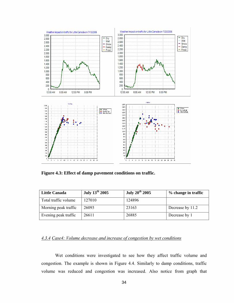
Figure 4.3: Effect of damp pavement conditions on traffic.
Little Canada July 13th 2005 July 20th 2005 % change in traffic
Total traffic volume 127010 124896
Morning peak traffic 26093 23163 Decrease by 11.2
Evening peak traffic 26611 26885 Decrease by 1
4.3.4 Case4: Volume decrease and increase of congestion by wet conditions
Wet conditions were investigated to see how they affect traffic volume and
congestion. The example is shown in Figure 4.4. Similarly to damp conditions, traffic
volume was reduced and congestion was increased. Also notice from graph that

35
congestion begins to occur at a lower volume which indicates reduction in the freeway
capacity. This reduction in capacity appears the cause of increased congestion.

36
Figure 4.4: Effect of wet pavement conditions on traffic.

37
Burnsville February 2nd 2005 February 14th 2005 % change of traffic
Total traffic volume 104683 104632
Morning peak traffic 21284 19793 Decrease by 7
Afternoon peak traffic 25003 25793 Increase by 3.1
4.3.5 Case 5: Changes in pavement conditions This is the case where changes from one kind of weather to another affected the
traffic volume and the congestion. From Figure 4.5, the morning and afternoon peak hour
volumes were reduced by 13.7% and 9.2%, respectively. The scatter graphs show that the
change in weather events increased congestion. This experiment suggests that any type of
weather events except dry conditions can affect traffic dynamics causing congestion.

38
Figure 4.5: Effect of different pavement conditions on the traffic volume. The volume/occupancy graphs of the corresponding days are also presented.
Little Canada January 5th 2005 January 12th 2005 % change of traffic
Total traffic volume 113963 107765
Morning peak traffic 24563 21194 Decrease by 13.7
Afternoon peak traffic 27565 25007 Decrease by 9.2
In summary, inclement weather conditions reduced the traffic volume while
increasing congestion during the peak hours. Traffic was not affected during the off-peak
hours. It was also observed that if the snow conditions are very severe, the traffic volume
drops considerably and the congestion was actually reduced or disappeared. The effect
damp and wet conditions were similar to snow conditions but a drastic drop of volume
that causes reduction in congestion was not observed. Finally, it was observed that when
the traffic volume was reduced during the peak hours by weather events, then more
traffic volume during the following off-peak hour was observed. This indicates that the
traffic flow shifts towards non-peak hour when weather events occur.

39
4.4 Impact of inclement weather conditions on travel time prediction
In order to analyze the impact of pavement conditions on travel time prediction, a
section of 17.5 miles from Maple Grove to Little Canada was used. Eq. 3.5 was used for
the computation of the percentage prediction error (PPE). The hypothesis is that PPE of
the time varying linear coefficient approach would be higher when inclement weather
conditions impacts the traffic dynamics. To analyze the travel time affected by weather
conditions, line graphs for the predicted travel time and the baseline travel time estimate
and its corresponding PPE values are compared. The calibrated travel time estimates (Eq.
3.4) at the same time are then plotted along with the predicted travel time values and the
baseline estimate of travel time to note any improvements. The weather impact on traffic
volume and volume/occupancy scatter graphs are presented to show the traffic
conditions.
In the following subsections, case by case analyses of various examples on
weather impact on travel time are shown. In all graphs, the legend “TV” denotes the time
varying linear coefficient approach, “Baseline” denotes actual travel time estimates, and
“TVWI” denotes travel time estimates with weather impact incorporated. The current
travel time predictor *( , )T t Δ in Eq. (2.3) is used to predict the travel time. In the
experiments, Δ was set to 5, 15, or 30 minutes, i.e., travel time prediction at 5, 15, or 30
minutes ahead. In the proceeding cases, only the prediction examples with 15Δ =
minutes are presented since the differences in performance can be more clearly observed
from the graphs. The historical information of 3 hours prior to the hour of prediction was
used to compute the time varying coefficients.
4.4.1 Case1: Effect of travel time prediction when weather conditions do not cause congestion As discussed in the previous section, severe snow conditions significantly
decrease the volume but reduction in the freeway capacity is not sufficient to cause
congestion. This case is shown in Figure 4.6. Once the traffic drops significantly the TV
travel time prediction model starts performing better sine the traffic is in a free flow state.

40
However it can be seen from the graph that during 5:00-6:00AM the traffic has not
dropped considerably, and thus the effect of weather impact can be seen on travel time
prediction for the hour. In the TVWI model, the change in the occupancy is used to adjust
the impact of inclement weather condition on travel time and the accuracy closely
approaches the baseline. The overall effect of significant drop in traffic due to severe
snow conditions is that the accuracy of travel time prediction by the TV model is well
maintained. The current travel time predictor is being used to predict the travel time 15
minutes into the future (Δ=15 minutes).
Effect of pavement conditions on travel time prediction for 01/17/2005
500
750
1000
1250
1500
5:00
5:20
5:40
6:00
6:20
6:40
7:00
7:20
7:40
8:00
8:20
8:40
9:00
Time instance
Trav
el ti
me
in s
econ
ds
TVBaselineTVWI

41
Figure 4.6: Traffic is affected by severe snow conditions that reduces the volume and avoids congestion and hence facilitates free flow conditions. The percentage prediction error of travel time is also negligible.
4.4.2 Case 2: Effect of travel time prediction by before-and-after weather events
The change in the pavement conditions can cause error in the prediction of travel
time as the prediction depends on the previous travel time information. If the weather
event changes from dry to snow, the TV prediction model underestimates the travel time
during the snow event. To illustrate this, note from Figure 4.7 that the pavement
conditions in the afternoon changes from dry conditions to snow. Congestion occurred
during the afternoon peak hours. Note from the travel time performance graph that TVWI
model performs better in comparison to the TV model under the change of weather
conditions since it incorporates the weather conditions.

42
Figure 4.7: Travel time prediction is affected by the snow conditions which causes congestion. The PPE graphs shows the error that occurs due to the change in weather.
Effect of pavement conditions on travel time prediction for 01/11/2005
500
750
1000
1250
1500
1750
15:00
15:25
15:50
16:15
16:40
17:05
17:30
17:55
18:20
18:45
Time instance of the day
Trav
el ti
me
in s
econ
ds
TV
Baseline
TVWI
Effect of calibration of weather impact on travel time prediction
-0.3-0.2
-0.10
0.10.2
0.30.4
15:00
15:25
15:50
16:15
16:40
17:05
17:30
17:55
18:20
18:45
Time instance
Perc
enta
ge p
redi
ctio
n er
ror PPETV
PPETVWI

43
4.4.3 Case3: Wet and damp pavement conditions in the morning peak time This case illustrates how the wet condition impacts travel time prediction. In
Figure 4.8, during the morning peak hours traffic volume was reduced due to wet
conditions but it caused congestion (significant increase of occupancy). As shown in the
travel time performance graphs of Figure 4.8, the TV prediction model underestimates
the travel time during the weather event and overestimates after the weather events. This
makes sense since it predicts the travel time based on the past data. Note from the TVWI
model that the rate of under and over estimate is significantly reduced since it
incorporates the weather condition. This case again demonstrates that incorporation of
weather impact to travel time prediction improves the accuracy of travel time prediction.

44
Figure 4.8: Travel time was affected by damp conditions. The damp conditions increase the travel time, and the TV prediction model underestimates the travel time. The TVWI model corrects the difference and improves the prediction accuracy.
Effect of pavement conditions on travel time prediction for 07/20/2005
500
750
1000
1250
1500
1750
5:00
5:20
5:40
6:00
6:20
6:40
7:00
7:20
7:40
8:00
8:20
8:40
9:00
Time instance
Trav
el ti
me
in s
econ
ds
TVBaselineTVWI
Effect of calibration of weather impact on travel time prediction
-0.4
-0.3
-0.2
-0.1
0
0.1
0.2
5:00
5:25
5:50
6:15
6:40
7:05
7:30
7:55
8:20
8:45
9:10
Time instance
Perc
enta
ge p
redi
ctio
n er
ror PPETV
PPETVWI

45
4.4.4 Case 4: The whole day is affected by snow Inclement weather conditions occur the whole day and can affect the travel time
prediction. As shown in Figure 4.9, traffic volume in this case tends to drop while
increasing travel time and congestion during the peak traffic hours. Note from the
performance graph that the TV prediction model consistently underestimates the travel
time in this case. The TVWI model corrects the error by incorporating the weather
conditions but it still underestimates the travel time in some instances.

46
Figure 4.9: Travel time is affected by snow conditions whole day. The snow conditions increases the travel time and the prediction tends to underestimate the travel time.
Effect of pavement conditions on travel time prediction for 01/20/2005
500750
10001250150017502000
5:00
5:30
6:00
6:30
7:00
7:30
8:00
8:30
9:00
16:05
16:35
17:05
17:35
18:05
18:35
Time instance
Trav
el ti
me
in s
econ
ds
TV
Baseline
TVWI
Effect of calibration of weather impact on travel time prediction
-0.4-0.3-0.2-0.1
00.10.20.30.4
5:00
5:30
6:00
6:30
7:00
7:30
8:00
8:30
9:00
16:0
5
16:3
5
17:0
5
17:3
5
18:0
5
18:3
5
Time instance
Perc
enta
ge p
redi
ctio
n er
ror PPETV
PPETVWI

47
4.4.5 Case 5: Multiple changes of weather changes during the day In this case, weather conditions vary during the day and change traffic conditions
and travel time. Figure 4.10 shows the condition changes from frost to snow, snow to
wet, and then wet to snow that occurs at the Little Canada site on Jan 12th 2005. The TV
model underestimated the travel time during the morning peak hours and overestimated
during the afternoon peak hours. This inconsistency is due to varying conditions. The
TVWI model corrects this error and closely approximates to the baseline estimates.

48
Figure 4.10: The TV travel time prediction is affected by changing weather conditions and is unable to predict the travel time accurately. The TVWI model reduces the error by incorporating the weather conditions.
Effect of pavement conditions on travel time prediction for 01/12/2005
500750
10001250150017502000225025002750
4:45
5:30
6:15
7:00
7:45
8:30
15:3
5
16:2
0
17:0
5
17:5
0
18:3
5
Time instance
Trav
el ti
me
in s
econ
ds
TV
Baseline
TVWI
Effect of calibration of weather impact on travel time prediction
-0.6
-0.4
-0.2
0
0.2
0.4
4:45
5:35
6:25
7:15
8:05
8:55
16:05
16:55
17:45
18:35
Time instance
Perc
enta
ge p
redi
ctio
n er
ror PPETV
PPETVWI

49
As shown through several cases the travel time is affected by changing weather
conditions. The error in the TV prediction model increases if the change in weather
conditions affects occupancy, since the TV prediction model uses past history to predict
future travel time. Weather is one of the factors that can change over time and affect the
travel time prediction. In this thesis it was demonstrated that the travel time predicted by
the TV model can be adjusted to incorporate weather impacts. In the formulation the
weather impact was estimated through increased occupancy and it was shown though
examples that the prediction error can be significantly reduced. Since all of our
experiments were done using past data, we were able to estimate and incorporate the
change of traffic conditions into the travel time prediction. In real world data, we assume
that the weather predictions can be obtained through the National Weather Service and
can be incorporated into the prediction model in terms of occupancy increase or decrease.

50
CHAPTER 5 : CONCLUSION
5.1 Conclusion The thesis first presented analyses on the weather impact on traffic utilizing
Mn/DOT RWIS and traffic data. According to the correlation coefficient study presented,
no strong correlation between the traffic and RWIS parameters was found. Next, the
effect of daily traffic volume was investigated. It was found that daily total volume under
weather events was only marginally affected (decreased). In most cases, the peak hour
traffic volume was reduced but reduced volume appeared during the off-peak hours as an
increase in volume. In order to study how weather impacts traffic during peak hours,
color coded visualization techniques were used, i.e., the traffic volume graphs were
generated with different color codes representing different pavement conditions and the
volume/occupancy scatter graphs were color coded according to morning and afternoon
peak hours and off-peak hours. The analysis of these graphs suggests that the traffic
volume generally drops during peak hours if a weather event occurs. The drop in the
traffic volume depends on the kind of weather event and the severity of the weather. It
was also observed that freeway capacity was reduced under weather events. In most
cases, congestion was increased during a weather event although the volume drops. This
happens because the weather event has reduced the freeway capacity but the trip demand
to use the freeway has not decreased accordingly. One exception was also observed.
During severe snow conditions the traffic volume drops considerably due to significant
reduction in trip demands. In those cases, congestion on the freeway was actually
reduced. The wet and damp conditions did not sufficiently reduce the trip demands
enough to ease congestion but the freeway capacity was reduced enough to cause a higher
level of congestion.
As the second part, the impact of weather events on the travel time prediction was
investigated using a time-varying linear coefficient (TV) model. Since the TV travel time
prediction model relies on the historical travel time information to estimate the future
travel time, the prediction errors were more significant under changing weather
conditions. It was observed that if the pavement conditions change from snow, damp or
wet to normal dry conditions then the TV model tends to overestimates the travel time.

51
On the other hand, if the pavement conditions change from dry to snow, damp or wet
conditions then the TV model tends to underestimates the travel time. This happens
because the prediction model assume the future travel condition is identical to the past
travel condition. In this thesis, an attempt was made to reduce the error induced by the
impact of weather changes. It was found that when the changes in occupancy of the
freeway under weather events and was compared to that of the normal dry conditions a
more accurate prediction of travel time was obtained. The calibration factor that has been
proposed in this thesis is based on the change in the occupancy that will occur due to the
impact of weather events. Various experiments that have been conducted for different
cases based on the theory and the experiments, it has been concluded that the error in the
travel time prediction increases during weather event and the travel time prediction can
be made more accurate if the change in estimated occupancy due to the weather event is
incorporated into the model.
5.2 Future Recommendations The weather impact on travel time was investigated using the color code for
different weather events and it showed the trends of traffic impact. However, one can also
try using the precipitation intensity and other weather related information to more
accurately model the impact of the weather events on traffic. Future work can also
include more specific studies on the measure of the severity of the weather events in
response to traffic impact. Such a measure would help formulate the drop in freeway
capacity and effect on congestion and could lead to more reliable prediction of future trip
times.
In the other part of this thesis we have used the change of occupancy as one of the
factors that can be used to adjust the travel time prediction during the change in weather
event. Another important area of for future work would be to predict the change in
occupancy if there is a change in weather events that are being predicted from such as the
National Weather Service. Once the change in occupancy can be predicted then the trip
time prediction can be done more reliably and this can help in trip planning. This also
relates to understanding of changes of trip demands and high way capacity by weather

52
events. If we can accurately predict the trip demands and the highway capacity, the
dependency of travel time prediction on the historical travel time can be avoided.

53
REFERENCES
Cambridge Systematics, Inc., Texas Transportation Institute 2005, Traffic congestion and
reliability: trends and advanced strategies for congestion mitigation, Federal highway
administration, Cambridge Systematics, Inc., Texas transportation institute, September
2005.
Chin, S. M., Franzese, O., Greene, D. L., Hwang, H. L., Gibson, R. C. (2004), Temporary
loss of highway capacity and impact on performance: phase 2, Oak ridge national
laboratory, Report no. ORLNL: TM-2004/209, November 2004.
Coifman, B. (1998), Vehicle reidentification and travel time measurement in real-time on
freeways using the existing loop detector infrastructure, Transportation Research Record
(1643):181-191, 1998
Cortes, C. E, Lavanya, R., Oh, J., Jayakrishnan, R. (2001), A general purpose
methodology for link travel time estimation using multiple point detection of traffic,
Department of Civil Engineering and institute of transportation studies, University of
California, Irvine, 2001.
Devore, J. L. (1995), Probability and Statistics for Engineering and the Sciences, 4th Ed,
Brooks/Cole Publishing Company, CA, USA, 1995.
Dion, F., Rakha H. (2003), Estimating Spatial Travel Time using Automatic Vehicle
Identification Data, Transportation Research Board (TRB) 2003
Goodwin, L. C., Best Practices for Road Weather Management, Federal Highway
Administration; May 2003.
Hall, F. and Persaud, B. N. (1989), Evaluation of speed estimates made with single-
detector data from freeway traffic management systems. Transportation Research Record,
1232:9-16, 1989.
Hastie, T., Tibshirani R., (1993), Varying coefficient models, Journal of the Royal
Statistical Society Series B, 55(4):757-796, 1993

54
Kirby, H. R., Watson, S. M., Dougherty, M. S. (1997), Should we use neural network or
statistical models for short-term motorway traffic forecasting?, International Journal of
Forecasting, 13(1):43-50, March 1997.
Kwon J., Coifman B., Bickel P. (2000), Day to day travel time trends and travel time
prediction from loop detector data, Transportation Research Record, 2000.
Kwon, T. M. (2004), TMC Traffic Data Automation for Mn/DOT’s Traffic Monitoring
Program, Mn/DOT; Report No. MN-RC-02004-29, July 2004.
Kwon T., Dhruv N. (2004), “Unified transportation sensor data format (UTSDF) for
efficient archiving and sharing of statewide transportation sensor data,” Proc. of the
Transportation Research Board 83nd Annual Meeting, Washington D.C., Jan. 2004.
Kwon T.M., Fleege E. (2000), “R/WIS Architecture for Integration and Expansion,”
Journal of the Transportation Research Board: Transportation Research Record 1700, pp.
1-4, The National Research Council, The National Academies, 2000.
Kwon, T. and Parsekar A. (2005), Deconvolution of vehicle inductance signature for
vehicle reidentification, Transportation Research Board 83nd Annual Meeting,
Washington D.C., Jan. 2005.
Nicholson, H., Swann, C. (1974), The prediction of traffic flow volumes based on
spectral analysis, Transportation Research, 8:533-538, 1974
Okutani I., Stephenades Y. J. (1984), Dynamic prediction of traffic volume through
Kalman Filtering, Transportation Research, 18(B):1-11, 1984
Lomax, T., Schrank, D. (2005), The 2005 urban mobility report, Texas Transportation
Institute, May 2005
Parsekar, A. (2004), Blind deconvolution of vehicle signature for travel time estimation,
November 2004.
Pisano, P., Goodwin, L.C. (2002), Surface transportation weather applications, ITE
2002Annual Meeting and Exhibit Compendium of Papers, 2002.

55
http://ops.fhwa.dot.gov/weather/best_practices/ITE2002_SurfTransWxAppl.pdf
Pisano, P. Ficek, M., Taylor, R (2004), Resources and further information: Weather and
ITS, U.S. Department of Transportation (US DoT), Federal Highway Administration
(FHWA), American Meteorological Society(AMS), Intelligent Transportation Society of
America (ITS America), January 2004
Rice, J., van Zweet, E. (2004), A simple and effective way for predicting travel times on
freeways, IEEE transactions on Intelligent Transportation Systems, 5(3):200-207,
September 2004.
Roess, R. P., McShane W. R., Prassas E. S. (1997), Traffic Engineering 2nd Edition,
Prentice-Hall, December 1997.
Schrader, C. C., Kornhauser, A. L., Friese, L. M. (2004), Using historical information in
forecasting travel times, Transportation Research Board, 2004.
Sun, C., Ritchie, S.G. (1999), Individual vehicle speed estimation using single loop
inductive waveform, Journal of Transportation Engineering, 1999.
Torday, A., Dumont, A. 2003, Link travel time estimation with probe vehicles in
signalized networks, SRTC, March 2003.
Transportation Engineers, Institute of (1999), Traffic Engineering Handbook 5th Edition,
Institute of Transportation Engineers, September 1999.
Transportation Research Board (1998), Special report 209: Highway capacity manual,
Transportation Research Board, 1998.
Yim, Y., Ygance, J., Drane, C. (2000), Travel Time Estimation on the San Francisco Bay
Area Network Using Cellular Phones as Probes, California PATH Draft Report D2000-
43.
Zhang, X., Rice, J. A. (2001), Short Term Travel Time Prediction Model using Time
Varying Coefficient Linear Model, Elsevier Reprint, March 2001.


![A Project Report Lalit[1]](https://static.fdocuments.net/doc/165x107/577cddb71a28ab9e78ad9566/a-project-report-lalit1.jpg)