Lagrangian torus fibrations

(notes in progress)

Jonny Evans

February 8, 2019

2

Contents

1 Introduction 5

2 The Arnol’d-Liouville theorem 72.1 Hamilton’s equations in 2D . . . . . . . . . . . . . . 72.2 Symplectic geometry . . . . . . . . . . . . . . . . . . 92.3 Integrable Hamiltonian systems . . . . . . . . . . . . 112.4 Liouville coordinates . . . . . . . . . . . . . . . . . . 132.5 The Arnol’d-Liouville theorem . . . . . . . . . . . . 152.6 Exercises . . . . . . . . . . . . . . . . . . . . . . . . 18

3 Hamiltonian torus actions 213.1 Global action-angle coordinates . . . . . . . . . . . . 213.2 Hamiltonian group actions . . . . . . . . . . . . . . . 223.3 Examples . . . . . . . . . . . . . . . . . . . . . . . . 273.4 Visible Lagrangian submanifolds . . . . . . . . . . . 323.5 Exercises . . . . . . . . . . . . . . . . . . . . . . . . 36

4 Focus-focus singularities 414.1 Flux map . . . . . . . . . . . . . . . . . . . . . . . . 414.2 Focus-focus singularities . . . . . . . . . . . . . . . . 444.3 Action coordinates . . . . . . . . . . . . . . . . . . . 474.4 Model neighbourhoods . . . . . . . . . . . . . . . . . 524.5 The Auroux system . . . . . . . . . . . . . . . . . . 53

4.6 Symington’s theorem . . . . . . . . . . . . . . . . . . 584.7 Exercises . . . . . . . . . . . . . . . . . . . . . . . . 59

5 Almost toric manifolds 635.1 Lagrangian torus fibrations . . . . . . . . . . . . . . 635.2 Operations . . . . . . . . . . . . . . . . . . . . . . . 645.3 Examples . . . . . . . . . . . . . . . . . . . . . . . . 745.4 Exercises . . . . . . . . . . . . . . . . . . . . . . . . 82

6 Ruan’s construction 856.1 Symplectic parallel transport . . . . . . . . . . . . . 856.2 Lagrangian torus fibrations . . . . . . . . . . . . . . 886.3 Quartic pencil . . . . . . . . . . . . . . . . . . . . . . 916.4 Exercises . . . . . . . . . . . . . . . . . . . . . . . . 96

7 Solutions to selected exercises 977.1 Chapter 1 . . . . . . . . . . . . . . . . . . . . . . . . 977.2 Chapter 5 . . . . . . . . . . . . . . . . . . . . . . . . 99

Chapter 1

Introduction

5

6 Chapter 1. Introduction

Chapter 2

The Arnol’d-Liouvilletheorem

2.1 Hamilton’s equations in 2D

The simplest nontrivial case of Hamilton’s equations is

p = −∂H∂q

, q =∂H

∂p. (2.1)

where (p(t), q(t)) is a path in the plane and H(p, q) is a function ofp and q. Physically, we could think of q as being position, p as beingmomentum and H as being energy1. Observe that

H =∂H

∂pp+

∂H

∂qq = qp− pq = 0,

1If H = p2

2m(the usual expression for kinetic energy) then Hamilton’s equa-

tions give the usual expression p = mq for momentum.

7

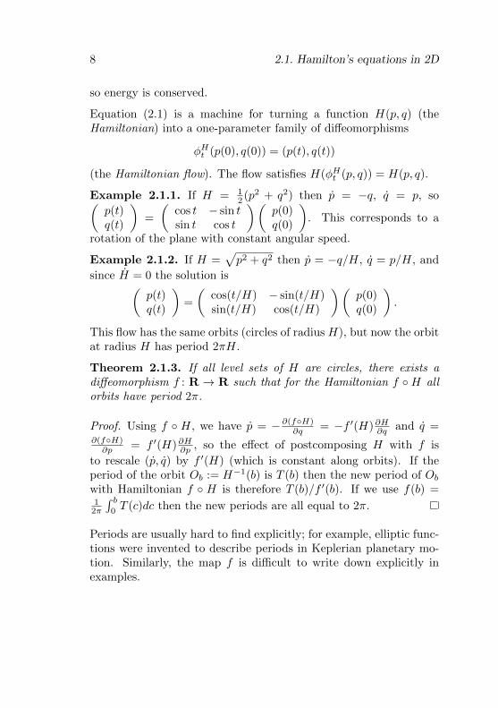
8 2.1. Hamilton’s equations in 2D

so energy is conserved.

Equation (2.1) is a machine for turning a function H(p, q) (theHamiltonian) into a one-parameter family of diffeomorphisms

φHt (p(0), q(0)) = (p(t), q(t))

(the Hamiltonian flow). The flow satisfies H(φHt (p, q)) = H(p, q).

Example 2.1.1. If H = 12 (p2 + q2) then p = −q, q = p, so(

p(t)q(t)

)=

(cos t − sin tsin t cos t

)(p(0)q(0)

). This corresponds to a

rotation of the plane with constant angular speed.

Example 2.1.2. If H =√p2 + q2 then p = −q/H, q = p/H, and

since H = 0 the solution is(p(t)q(t)

)=

(cos(t/H) − sin(t/H)sin(t/H) cos(t/H)

)(p(0)q(0)

).

This flow has the same orbits (circles of radius H), but now the orbitat radius H has period 2πH.

Theorem 2.1.3. If all level sets of H are circles, there exists adiffeomorphism f : R → R such that for the Hamiltonian f H allorbits have period 2π.

Proof. Using f H, we have p = −∂(fH)∂q = −f ′(H)∂H∂q and q =

∂(fH)∂p = f ′(H)∂H∂p , so the effect of postcomposing H with f is

to rescale (p, q) by f ′(H) (which is constant along orbits). If theperiod of the orbit Ob := H−1(b) is T (b) then the new period of Obwith Hamiltonian f H is therefore T (b)/f ′(b). If we use f(b) =1

2π

∫ b0T (c)dc then the new periods are all equal to 2π.

Periods are usually hard to find explicitly; for example, elliptic func-tions were invented to describe periods in Keplerian planetary mo-tion. Similarly, the map f is difficult to write down explicitly inexamples.

9

Theorem 2.1.4. In a 1-parameter family of closed orbits Ob, b ∈ R,of a Hamiltonian system, the period of Ob is d

db

∫Obpdq.

Remark 2.1.5. This means that f(b) = 12π

∫Obpdq is another way of

writing the function we found in Theorem 2.1.3).

Proof. Assume for simplicity2 that we have coordinates (p, q), withq ∈ R/2πZ, such that the orbits have the form Ob := (pb(q), q) :q ∈ R/2πZ for some functions pb. Then

T (b) =

∫ 2π

0

dt

dqdq =

∫ 2π

0

dq

q

=

∫ 2π

0

dq

∂H/∂pb=

∫ 2π

0

∂pb∂H

dq =d

db

∫ 2π

0

pdq.

Our goal in this first lecture is to generalise these observations toHamiltonian systems in higher dimensions. It will be convenient tointroduce the language of symplectic geometry.

2.2 Symplectic geometry

Definition 2.2.1. Let X be a manifold and ω a 2-form. Definea map3 [ : Γ(TX) → Γ(T ∗X) by [(V ) = ιV ω. We say that ω isnondegenerate if [ is an isomorphism, in which case we write ] forits inverse. A symplectic form is a closed, nondegenerate 2-form.

Definition 2.2.2. Given a smooth function H : X → R and a sym-plectic form ω on X, we get a vector field VH := −](dH) (i.e.ιVHω = −dH). We call such vector fields Hamiltonian. The flowφHt along VH is called a Hamiltonian flow.

2One can always find coordinates (p, q) in which the orbits have this form.3Γ(TX) denotes the space of vector fields and Γ(T ∗X) the space of 1-forms.

10 2.2. Symplectic geometry

Example 2.2.3. Let ω = dp∧dq on X = R2. Then, if (p(t), q(t)) =φHt (p(0), q(0)), we have VH = (p, q) and ιVHω = pdq − qdp =−∂H∂p dp−

∂H∂q dq so we recover Hamilton’s equations (2.1).

Lemma 2.2.4. A Hamiltonian flow φHt satisfies (φHt )∗ω = ω and(φHt )∗H = H.

Proof. We first show that the Lie derivatives LVHω and LVHH van-ish. For this, we use Cartan’s formula LV η = ιV dη + dιV η for theLie derivative of a differential form η along a vector field V . Wehave

LVHω = dιVHω + ιVHdω = −ddH = 0,

as dω = 0 and ιVHω = −dH, and

LVHH = ιVHdH = −ω(VH , VH) = 0,

as ω is antisymmetric.

Now note that ddt (φ

Ht )∗ω = (φHt )∗L(φHt )∗VHω and (φHt )∗VH = VH ,

so LVHω = 0 implies ddt (φ

Ht )∗ω = 0, so (φHt )∗ω = ω. Similarly, the

fact that (φHt )∗H = H follows from the vanishing of LVHH.

Remark 2.2.5. Note that if H is also allowed to depend explicitlyon t (a non-autonomous Hamiltonian flow) then the previous argu-ment for conservation of energy breaks down. Nonetheless, the flowpreserves the symplectic form.

Lemma 2.2.6. The Lie bracket of two Hamiltonian vector fieldsVF and VG is the Hamiltonian vector field VF,G, where F,G =ω(VF , VG).

Proof. We have ι[VF ,VG]ω = [LVF , ιVG ]ω. Since VF is symplectic,the term ιVGLVFω vanishes. Expanding the remaining term usingCartan’s formula, and remembering that dιVGω = −ddG = 0, weget ι[VF ,VG]ω = dιVF ιVGω. Since ιVF ιVGω = −ω(VF , VG) this tells usthat [VF , VG] = Vω(VF ,VG) as required.

11

Definition 2.2.7. The quantity F,G is called the Poisson bracketof F and G. We say that F and G Poisson commute if F,G = 0.

Lemma 2.2.8 (Exercise). If F and G are smooth functions and wedefine Ft(x) := F (φGt (x)) then Ft = G,Ft.

2.3 Integrable Hamiltonian systems

Suppose we have a symplectic manifold (X,ω) and a map H =(H1, . . . ,Hn) : X → Rn for which the components H1, . . . ,Hn sat-isfy Hi, Hj = 0 for all pairs i, j. In what follows, we will assumethat the vector fields VHi can be integrated for all time, so that theflows φHit are defined for all t ∈ R. The flows φH1

t1 , . . . , φHntn commute

with one another and hence define an action of the group Rn on X.We call this a Hamiltonian Rn-action.

Example 2.3.1. Consider the R2-action on R2 where (s, t) acts by(s, t) · (x0, y0) = (x0 +s, y0 + t) = φxt φ

ys(x0, y0). Even though φxt and

φys define Hamiltonian R-actions which commute, this example isnot a Hamiltonian R2-action because the Poisson bracket x, y = 1is not zero (i.e. they do not Poisson-commute).

More generally, for a Lie group G with Lie algebra g, a Hamilto-nian G-action is a G-action in which every one-parameter subgroup

exp(tξ) acts as a Hamiltonian flow φHξt , and the assignment ξ 7→ Hξ

is a Lie algebra map (i.e. H[ξ1,ξ2] = Hξ1 , Hξ2.

Definition 2.3.2. A submanifold L of a symplectic manifold (X,ω)is called isotropic if ω vanishes on vectors tangent to L. If dimX =2n then dimL ≤ n for an isotropic submanifold L (exercise) and wesay that L is Lagrangian if L is isotropic and dimL = n.

Lemma 2.3.3. The orbits of a Hamiltonian Rn-action on a sym-plectic manifold (X,ω) are isotropic. As a consequence, if X con-

12 2.3. Integrable Hamiltonian systems

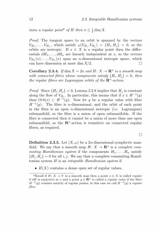
tains a regular point4 of H then n ≤ 12 dimX.

Proof. The tangent space to an orbit is spanned by the vectorsVH1

, . . . , VHn , which satisfy ω(VHi , VHj ) = Hi, Hj = 0, so theorbits are isotropic. If x ∈ X is a regular point then the differ-entials dH1, . . . , dHn are linearly independent at x, so the vectorsVH1(x), . . . , VHn(x) span an n-dimensional isotropic space, whichcan have dimension at most dimX/2.

Corollary 2.3.4. If dimX = 2n and H : X → Rn is a smooth mapwith connected fibres whose components satisfy Hi, Hj = 0, thenthe regular fibres are Lagrangian orbits of the Rn-action.

Proof. Since Hi, Hj = 0, Lemma 2.2.8 implies that Hj is constantalong the flow of VHi . In particular, this means that if x ∈ H−1(y)then Orb(x) ⊂ H−1(y). Now let y be a regular value with fibreH−1(y). The fibre is n-dimensional, and the orbit of each pointin the fibre is an open n-dimensional isotropic (i.e. Lagrangian)submanifold, so the fibre is a union of open submanifolds. If thefibre is connected then it cannot be a union of more than one opensubmanifold, so the Rn-action is transitive on connected regularfibres, as required.

Definition 2.3.5. Let (X,ω) be a 2n-dimensional symplectic man-ifold. We say that a smooth map H : X → Rn is a complete com-muting Hamiltonian system if the components H1, . . . ,Hn satisfyHi, Hj = 0 for all i, j. We say that a complete commuting Hamil-tonian system H is an integrable Hamiltonian system if

• H(X) contains a dense open set of regular values,

4Recall if H : X → Y is a smooth map then a point x ∈ X is called regularif dH is surjective at x and a point y ∈ Rn is called a regular value if the fibreH−1(y) consists entirely of regular points; in this case we call H−1(y) a regularfibre.

13

• H is proper (preimages of compact sets are compact) and hasconnected fibres.

The first assumption rules out trivial examples; the properness con-dition ensures that the flows of the vector fields VH1 , . . . , VHn existfor all time.

We write ΦHt := φH1t1 · · ·φ

Hntn for this Rn-action and Orb(x) for its

orbit through x ∈ X. Each orbit is isotropic and the orbit of aregular point is Lagrangian.

2.4 Liouville coordinates

Definition 2.4.1. A local Lagrangian section of an integrable Hamil-tonian system H : X → Rn is a Lagrangian embedding σ : U → Xwhere U ⊂ H(X) is an open set and H σ(b) = b for all b ∈ U .

Lemma 2.4.2 (Exercise). There always exists a local Lagrangiansection through any regular point x.

Theorem 2.4.3 (Liouville coordinates). Let H : X → Rn be anintegrable Hamiltonian system and σ : U → X be a local Lagrangiansection. Define

Ψ: U ×Rn → X, Ψ(b, t) = ΦHt (σ(b)).

Then Ψ is both an immersion and a submersion and Ψ∗ω =∑dbi∧

dti, where (b1, . . . , bn) are the standard coordinates on U ⊂ Rn. Thismeans that (b1, . . . , bn, t1, . . . , tn) provide local symplectic coordinateson a neighbourhood of σ(U); we call these Liouville coordinates.

Proof. • Ψ∗∂bi and Ψ∗∂bj are tangent to ΦHt (σ(U)), which isthe image of a Lagrangian under a series of Hamiltonian flows,hence Lagrangian. Therefore ω(Ψ∗∂bi ,Ψ∗∂bj ) = 0.

14 2.4. Liouville coordinates

• Ψ∗∂ti = VHi , so

ω(Ψ∗∂ti ,Ψ∗∂tj ) = ω(VHi , VHj ) = Hi, Hj = 0.

• ω(Ψ∗∂bi ,Ψ∗∂tj ) = dHj(Ψ∗∂bi), and, since (Hj Ψ)(b, t) = bj(as the flow along Ψt preserves the level sets of Hj) we havedHj(Ψ∗(∂bi)) = dbj(∂bi) = δij . Therefore Ψ∗ω =

∑ni=1 dbi ∧

dti = ω0.

Note that this implies that Ψ is both an immersion and a submersion(if it failed to be an immersion or a submersion at some point thenΨ∗ω would be degenerate there).

Definition 2.4.4. We call the subset Λ := Ψ−1(σ(U)) ⊂ U×Rn theperiod lattice. It is a Lagrangian submanifold with respect to

∑dbi∧

dti since Ψ is a local symplectomorphism and σ(U) is Lagrangian.We say that the period lattice is standard if it is equal to U×(2πZ)n.

Example 2.4.5. The period lattice in Example 2.1.1 is standard,while in Example 2.1.2 it is (r, 2πr) : r > 0, where U = R>0 isthe set of positive radii and σ(r) = r.

Example 2.4.6. Consider the Hamiltonian system on R2 whoselevel sets are shown in the figure below. This Hamiltonian generatesan R-action whose orbits are: the fixed points; the two separatrices;the closed loops. The separatrices have infinite period (it takes in-finitely long to flow around them). If we take as Lagrangian sectionthe line segment indicated in red then the period lattice looks likethe figure on the right.

15

The justification for the name period lattice comes from the followingtheorem:

Lemma 2.4.7 (Exercise). For each b ∈ U , the intersection Λb =Λ∩ (b×Rn) is a lattice in Rn, that is a discrete subgroup of Rn.The rank of the lattice is lower semicontinuous as a function of b,that is, b has a neighbourhood V such that rank(Λb′) ≥ rank(Λb)for all b′ ∈ V .

Example 2.4.8. In Example 2.4.6, the period lattice for most orbitsis isomorphic to Z, but where U intersects the separatrix orbit theperiod lattice is the zero lattice.

Recall the following result from differential topology.

Theorem 2.4.9. If Λ ⊂ Rn is a lattice then there is a basis e1, . . . , enof Rn such that Λ is the Z-linear span of the vectors e1, . . . , ek forsome k ≤ n.

Our next goal is to find a local diffeomorphism G : U → Rn suchthat G H has standard period lattice.

2.5 The Arnol’d-Liouville theorem

Theorem 2.5.1 (Little Arnol’d-Liouville theorem). Let H : X →Rn be an integrable Hamiltonian system and σ : U → X be a localLagrangian section. Each orbit Orb(σ) is diffeomorphic to

(Rk/Zk

)×

Rn−k for some k. In particular, if Orb(σ) is compact then it is atorus.

Proof. The action of Rn defines a diffeomorphism Rn/Λσ → Orb(σ).Since Λσ is a lattice, the result follows from the classification of lat-tices in Theorem 2.4.9.

We now focus attention on a neighbourhood of a compact (torus)orbit. By Lemma 2.4.7, all nearby orbits are also tori. We will

16 2.5. The Arnol’d-Liouville theorem

shrink the domain U of our local Lagrangian section so that allorbits through σ(U) are compact and, moreover, so that U is a disc.

Theorem 2.5.2 (Action-angle coordinates). There is a local changeof coordinates G : U → Rn such that G H : H−1(U) → Rn gen-erates a Hamiltonian torus action on H−1(U). In other words,the period lattice Λ is standard, equal to U × (2πZ)n and the mapΨ: U ×Rn → X defined in Theorem 2.4.3 descends to give a sym-plectomorphism U × (R/2πZ)n → H−1(U).

Proof. The following proof is due to Duistermaat [5].

For each b ∈ U , let 2πW1(b), . . . , 2πWn(b) ∈ Rn be a collectionof vectors (smoothly varying in b) which span the lattice of periodsΛb. We wish to find functions G1(b1, . . . , bn), . . . , Gn(b1, . . . , bn) suchthat ιWiω = −d(Gi H). If Wi =

∑αijVHj then this is equivalent

to requiring ∂Gi∂bj

= αij . By the Poincare lemma, we can find such

functions Gi provided∂αij∂bk

=∂αik∂bj

, (2.2)

so it remains to check this identity.

Let Ψ: U×Rn → X be the Liouville coordinates and Λ = Ψ−1(σ(U))be the period lattice. Since Ψ is symplectic and σ(U) is Lagrangian,Λ is Lagrangian. Moreover, Λ is a union of sheets, each tracedout by a single lattice point. For example, (b,Wi(b)) : b ∈ Utraces out a Lagrangian sheet for each i. In coordinates, this is(b1, . . . , bn, αi1(b), . . . , αin(b)) : b ∈ U, which is Lagrangian ifand only if Equation (2.2) holds.

Definition 2.5.3. The Liouville coordinates associated to the new,periodic Hamiltonian system are called action-angle coordinates. Moreprecisely, the new Hamiltonians G1 H, . . . , Gn H are called actioncoordinates and the new 2π-periodic conjugate coordinates t1, . . . , tnare called angle coordinates.

17

Corollary 2.5.4 (Big Arnol’d-Liouville theorem). If H : M → Rn

is an integrable Hamiltonian system and Orb(p) is a compact or-bit then Orb(p) is a torus and there is a neighbourhood of Orb(p)symplectomorphic to U × Tn, where U ⊂ Rn is an open ball andthe symplectic form is given by

∑ni=1 dbi ∧ dti. Under this symplec-

tomorphism, the orbits of the original system are sent to the torib × Tn.

18 2.6. Exercises

2.6 Exercises

Exercise 2.6.1. Let (p, q) be coordinates on R × S1 (with q ∈R/2πZ) and let ω = dp ∧ dq. Consider the Hamiltonian H =12p

2 + cos q. Find its critical points and the Hessian of H at thecritical points. Sketch the level sets of H and identify the orbitsof φHt . Physically, this Hamiltonian system corresponds to a pen-dulum swinging in a uniform gravitational field; q is the angulardisplacement from the downward vertical. What is the physical in-terpretation of the orbits you identified? Around the critical point

(0, 0), make the small angle approximation cos q ≈ 1− q2

2 and solvethe resulting Hamiltonian system. Verify Galileo’s observation thatthe period of a pendulum with small oscillation is independent of itsinitial angular displacement. ** Find the period precisely in termsof elliptic integrals.

Exercise 2.6.2. Show that in the local modelH : Rn×(R/2πZ)n →Rn, H(p, q) = p, the action coordinates of the orbit Ob := H−1(b)

are(

12π

∫c1λ0, . . . ,

12π

∫cnλ0

)where λ0 =

∑nk=1 pkdqk and ck is the

loop p = 0, qi = 0 for i 6= k. Verify that the same is true for anyλ satisfying dλ = ω.

Exercise 2.6.3. Consider the unit 2-sphere (S2, ω) where ω is thearea form. By comparing infinitesimal area elements, show thatthe projection map from S2 to a circumscribed cylinder is area-preserving5. Let H : S2 → R be the height function H(x, y, z) = z(thinking of S2 embedded in the standard way in R3). Show thatH is an action coordinate.

Exercise 2.6.4. A symplectic vector space is a vector space X to-gether with a nondegenerate alternating bilinear form ω (like thetangent space of a symplectic manifold). A subspace Y ⊂ X iscalled:

5If Cicero is to be believed, a diagram representing this theorem was engravedon the tomb of Archimedes (who proved it).

19

• symplectic if ω|Y is symplectic;

• isotropic if ω|Y = 0.

Given a subspace Y , define the symplectic orthogonal complement

Y ω := v ∈ X : ω(v, w) = 0 for all w ∈ Y .

A basis p1, q1, . . . , pn, qn for X is called symplectic if ω(pj , qk) = δjkand ω(pj , pk) = ω(qj , qk) = 0 for all j, k. Show that: a) any sym-plectic vector space admits a symplectic basis and hence has evendimension. (Hint: Work inductively using symplectic orthogonalcomplement.) b) if Y is isotropic then Y ⊂ Y ω. Deduce thatdimY ≤ n.

Exercise 2.6.5. If F and G are two functions on a symplectic man-ifold, define Ft(x) = F (φGt (x)) and show that Ft = G,Ft.

Exercise 2.6.6. Recall that the flows along two vector fields com-mute if and only if the Lie bracket of the vector fields vanishes.Deduce that two Hamiltonian flows φFt and φGt commute if and onlyif the Poisson bracket F,G is locally constant.

Exercise 2.6.7. Darboux’s theorem states that for any symplec-tic 2n-manifold (X,ω) and any point x ∈ X, there are coordinates(p1, q1, . . . , pn, qn) centred on x such that ω =

∑dpi ∧ dqi in these

coordinates. We will prove this by induction. This proof is fromArnol’d’s book [1, Section 43.B] (look there if you get stuck). As sooften in geometry proofs, we will tacitly pass to a smaller neighbour-hood at various points in the proof. a) Pick a function p1 and let Nbe a submanifold passing through x, transverse to the vector fieldVp1 in a neighbourhood of x. For points in a neighbourhood of x,define q1 to be the unique number such that φp1−q1(x) ∈ N . Computethe Lie derivative LVp1 q1 and show that p1, q1 = 1. Deduce thatthe flows φp1t and φq1t commute. Deduce Darboux’s theorem in thecase n = 1. b) Let M = p1 = q1 = 0. Why is TxM a symplecticsubspace of TxX? Why does this means that M is a symplecticsubmanifold in a neighbourhood of x? c) By induction, M admits

20 2.6. Exercises

Darboux coordinates (a2, b2, . . . , an, bn) in a neighbourhood of x.Any point x′ in a neighbourhood of x can be written uniquely asx′ = φp1s φ

q1t (m(x′)) with m(x′) ∈M , so defining pk(x′) = ak(m(x′))

and qk(x′) = bk(m(x′)) we get coordinates (p1, q1, . . . , pn, qn) on aneighbourhood of x. Check that these are Darboux coordinates, inother words: pj , qk = δjk, pj , pk = qj , qk = 0 for all j, k.

Exercise 2.6.8. There always exists a local Lagrangian sectionthrough any regular point x of an integrable Hamiltonian system.

Exercise 2.6.9. Suppose thatH : X → R is a Hamiltonian functionand L ⊂ X is a Lagrangian submanifold such that L ⊂ H−1(c) forsome c ∈ R. Prove that φHt (x) ∈ L for all x ∈ L, t ∈ R, i.e. that Lis invariant under the Hamiltonian flow of H.

Exercise 2.6.10. Let (X,ω) be a symplectic 2n-manifold, B be ann-manifold and let π : X → B be a proper submersion with con-nected Lagrangian fibres. Let (b1, . . . , bn) be local coordinates onB. Prove that b1 π, . . . , bn π Poisson commute, and deduce thatthe fibres of π are Lagrangian tori. This is the reason the words La-grangian torus fibration and integrable Hamiltonian system are oftenconflated (Hint: Use Exercise 2.6.9.)

The final two questions use the fact that the Liouville map Ψ is alocal diffeomorphism.

Exercise 2.6.11. Let H : X → Rn be an integrable Hamiltoniansystem and σ : U → X be a local Lagrangian section. Let Λ bethe associated period lattice. Prove that, for each point b ∈ U , theintersection Λb := Λ ∩ (b ×Rn) is a sublattice of Rn (that is, adiscrete subgroup of Rn).

Exercise 2.6.12. Let H : X → Rn be an integrable Hamiltoniansystem and σ : U → X be a local Lagrangian section. Show that thefunction U → Z, b 7→ rank(Λb), is lower semi-continuous (in otherwords, there is an open neighbourhood V of b such that, for b′ ∈ V ,rank(Λb′) ≥ rank(Λb)).

Chapter 3

Hamiltonian torusactions

3.1 Global action-angle coordinates

We saw in the last chapter that if H : X → Rn is a integrable Hamil-tonian system and b is a regular value then we can postcompose witha local change of coordinates G on a neighbourhood U of b to geta new system G H such that G H generates a torus action onH−1(U). The components G1 H, . . . , Gn H are called action co-ordinates and the angular coordinates on the torus fibres are calledangle coordinates. The following lemma tells us that when we haveem globally defined action-angle coordinates on X, the whole Hamil-tonian system can be recovered just from the image of X under theaction coordinates.

Lemma 3.1.1. Assume that F : X → Rn and G : Y → Rn areintegrable Hamiltonian systems such that U := F (X) and V :=

21

22 3.2. Hamiltonian group actions

G(Y ) consist only of regular values. Assume that F and G are actioncoordinates in each case and that we are given global Lagrangiansections σ : U → X and τ : V → Y . Suppose there is an integralaffine transformation A : Rn → Rn such that A(U) = V . There isa symplectomorphism Φ: X → Y such that G Φ = A F ; we callsuch a symplectomorphism fibred.

This is a wonderful compression of information: to reconstruct a2n-dimensional space, all we need is a subset of Rn. For example,if n = 2, 3, this brings 4- and 6-dimensional spaces into the range ofvisualisation. The goal of the rest of this book is to exploit this inincreasing levels of generality.

• In this chapter, we will keep the assumption that there areglobal action-angle coordinates, but allow for critical points.This will lead us to the study of toric manifolds.

• In Chapter 4, we will drop the assumption that there are globalaction-angle coordinates and see what remains. We will intro-duce more general singularities (focus-focus singularities) andstudy the asymptotics of action-angle coordinates in the neigh-bourhood of a singular fibre.

• In Chapter 5, we will combine what we have done so far tovisualise a range of interesting 4- and 6-dimensional manifolds.

• In Chapter 6, we will explain a construction due to Ruan ofintegrable Hamiltonian systems on projective varieties admit-ting toric degenerations. The singularities of these examplesare still poorly-understood.

3.2 Hamiltonian group actions

One way of stating the Arnol’d-Liouville theorem is that, after asuitable change of coordinates in the target, the Rn-action gener-ated by the Hamiltonian vector fields VH1

, . . . , VHn actually factors

23

through a Tn-action. We now work backwards, assuming that wehave a globally-defined torus action, even on the non-regular fibres,and see what kinds of singularities can occur.

Definition 3.2.1. Let H : X → Rn be an integrable Hamiltoniansystem such that the Hamiltonian Rn-action ΦHt factors through aHamiltonian Tn-action, that is ΦHt = id for any t ∈ (2πZ)n. Thenwe call H the moment map for the torus action; this is a synonymfor having globally defined action coordinates. We often write µ fora moment map, to distinguish it from a system where the periodlattice is not standard.

We saw in Lemma 3.1.1 that the image of a moment map deter-mines the Hamiltonian system completely up to fibred symplecto-morphism, at least if there are no critical points and there is a globalLagrangian section. We therefore concentrate on the image µ(X) ofthe moment map, which we will call the moment image or momentpolytope. The Atiyah-Guillemin-Sternberg convexity theorem tellsus that µ(X) indeed a polytope. Before stating this theorem, werecall some basic definitions.

Definition 3.2.2. A rational convex polytope P is a subset of Rn

defined as the intersection of a finite collection of half-spaces Sα,b =x ∈ Rn : α1x1 + · · · + αnxn ≤ b with α1, . . . , αn ∈ Q andb ∈ Rn. We say that P is a Delzant polytope if it is a convexrational polytope such that every point on a k-dimensional facet hasa neighbourhood isomorphic (via an integral affine transformation)to a neighbourhood of the origin in the polytope [0,∞)n−k ×Rk.

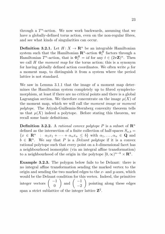
Example 3.2.3. The polygon below fails to be Delzant: there isno integral affine transformation sending the marked vertex to theorigin and sending the two marked edges to the x- and y-axes, whichwould be the Delzant condition for this vertex. Indeed, the primitive

integer vectors

(−10

)and

(−1−2

)pointing along these edges

span a strict sublattice of the integer lattice Z2.

24 3.2. Hamiltonian group actions

•

Theorem 3.2.4 (Atiyah, Guillemin-Sternberg, Delzant). Let (X,ω)be a symplectic 2n-manifold and µ : X → Rn a moment map for aHamiltonian Tn-action.

1. The image ∆ := µ(X) is a Delzant polytope.

2. If X is compact, then ∆ is the convex hull of µ(x) : x ∈Fix(X), where Fix(X) is the set of fixed points of the torusaction.

3. For any Delzant polytope ∆ ⊂ Rn there exists a symplectic 2n-manifold X∆ and a map µ : X∆ → Rn with µ(X∆) = ∆ suchthat µ generates a Hamiltonian Tn-action. Moreover, X∆ isa projective variety. Such varieties are often called projectivetoric varieties.

4. The moment polytope determines X,µ up to fibred symplecto-morphism.

We will not prove this theorem, and will focus instead on extractinggeometric information about X from the moment polytope.

Example 3.2.5. Consider the n-torus action on Cn given by

(z1, . . . , zn) 7→ (eit1z1, . . . , eitnzn).

25

This is Hamiltonian, with moment map

µ(z1, . . . , zn) =

(1

2|z1|2, . . . ,

1

2|zn|2

).

The image of the moment map is the nonnegative orthant. This is amanifold with boundary and corners: the µ-preimage of a boundarystratum of codimension k is an (n − k)-dimensional torus. For ex-ample, the preimage of the vertex is a single fixed point (the origin),the preimage of a point on the positive x1-axis is a circle with fixedradius in the z1-plane, the preimage of a point on the interior of thex1x2-plane is a 2-torus, and so forth.

C2 C3

Remark 3.2.6. The critical values of µ are precisely the boundarypoints of the moment polytope. The boundary is stratified intofacets of dimension 0 (vertices), 1 (edges), 2 (faces), etc, so we canclassify the critical values according to the dimension of the stratumto which they belong. By definition, any Delzant polytope is locallyisomorphic to Rk × [0,∞)n−k in a neighbourhood of a point in a k-dimensional facet. In Example 3.2.5, we have found a system whosemoment image is [0,∞)n−k, so by Theorem 3.2.4(4), this means thatthe integrable Hamiltonian system in a neighbourhood of a criticalpoint living over a k-dimensional facet is fibred-symplectomorphicto the system

µ : Rk × (S1)k ×Cn−k → Rn,

µ(p, q, zk+1, . . . , zn) =

(p,

1

2|zk+1|2, . . . ,

1

2|zn|2

).

26 3.2. Hamiltonian group actions

Such singularities are called toric1 and the set of all toric singularitiesis often called the toric boundary of X. It is not a boundary in theusual sense: it is a union of submanifolds of codimension 2. Instead,considering X as a projective variety, it is the boundary in the senseof algebraic geometry: it is a divisor, and is often called the toricdivisor.

Our ultimate goal is to see features of the geometry laid bare viathe moment map. As an example of what we have in mind, here is anice way to understand the genus 1 Heegaard decomposition of the3-sphere using the moment map for C2.

Example 3.2.7. Let µ : C2 → R2 be the moment map from Ex-ample 3.2.5. The preimage of the (red) line segment x1 + x2 = 1

2 ,x1, x2 ≥ 0, is the subset S := (z1, z2) ∈ C2 : |z1|2 + |z2|2 = 1,that is the unit 3-sphere. The fibre T := µ−1

(14 ,

14

)is a torus with

T ⊂ S. We can see that T separates S into two pieces S1, S2, andit is also easy to see that each piece is homeomorphic to a solidtorus S1 × D2: the “core circles” of these solid tori are the fibress1 = µ−1

(12 , 0), s2 = µ−1

(0, 1

2

)where the line segment intersects

the x1- and x2-axes.

S

S1

S2 •T

•

•

s1

s2

si

T

Si

1In fact, it is a theorem of Eliasson [6] and Dufour–Molino [4] that toric sin-gularities can be characterised purely in terms of the Hessian of the Hamiltoniansystem at the singular point. They call such critical points elliptic.

27

3.3 Examples

Example 3.3.1. We saw in Exercise 2.6.3 that the height functionon the unit 2-sphere in R3 generates a Hamiltonian circle action (i.e.T 1-action). The image of the moment map is the interval [−1, 1].One can form more examples by taking products: we get a Tn-actionon (S2)n, whose moment map is µ((x1, y1, z1), . . . , (xn, yn, zn)) =(z1, . . . , zn), with image [−1, 1]n. For example, the moment imagefor S2 × S2 is a square, for S2 × S2 × S2 it is a cube.

Example 3.3.2. If we take S2 with the area form λω (where ω isthe form giving area 4π) then the rescaled height function λz is amoment map for the circle action which rotates around the z-axiswith period 2π. The moment image is [−λ, λ].

Definition 3.3.3 (Affine length). If ` : [0, L]→ Rn is a line segment

of the form `(t) = at + b with a =

(a1

a2

)∈ Z2, gcd(a1, a2) = 1

and b ∈ Rn then we say ` is a rational line segment and the affinelength of ` is defined to be L.

Example 3.3.4. In the polygon below, the vertical edge has affinelength 2 and the other two edges both have affine length 1.

Lemma 3.3.5. If ` : [0, L] → Rnis a rational line segment whoseimage is an edge of the moment polytope then µ−1(`([0, L])) is a

28 3.3. Examples

symplectic sphere of symplectic area 2πL.

Proof. By Theorem 3.2.4(4), the preimage of such an edge is pre-cisely symplectomorphic to

(S2, Lω2

)with a rescaling of its height

function by L/2, by comparing with Example 3.3.2.

Example 3.3.6. Consider the complex projective n-space CPn,with homogeneous coordinates [z1 : · · · : zn+1]. This has a torusaction [z1 : · · · : zn+1] 7→ [eit1z1 : · · · : eitnzn : zn+1] which isHamiltonian, for the Fubini-Study form ω, with moment map

µ([z1 : · · · : zn+1] =

(1

2

|z1|2

|z|2, . . . ,

1

2

|zn|2

|z|2

),

where |z|2 =∑n+1i=1 |zi|2. The moment image is the simplex

(x1, . . . , xn) ∈ Rn : x1, . . . , xn ≥ 0, x1 + · · ·+ xn ≤ 1.

For example, µ(CP2) and µ(CP3) are drawn below. In each case,the hyperplane at infinity [z1 : · · · : zn : 0] projects via µ to thefacet x1 + · · ·+ xn = 1 of the simplex.

CP2 CP3

Example 3.3.7. The tautological bundle over CP1 is the variety

O(−1) := (x, y, [a : b]) ∈ C2 ×CP1 : ay = bx.

This has a holomorphic projection π : O(−1) → CP1, π(x, y, [a :b]) = [a : b], which exhibits it as the total space of a holomorphicline bundle over CP1. This is a fancy way of saying that π−1([a : b])

29

is a complex line (specifically (x, y) ∈ C2 : ay = bx ⊂ C2) forall [a : b] ∈ CP1. The symplectic form ωC2 ⊕ ωCP1 on C2 × CP1

pulls back to a symplectic form on O(−1), with respect to which thefollowing T 2-action is Hamiltonian:

(x, y, [a : b]) 7→ (eit1x, eit2y, [eit1a : eit2b]).

The moment map is

µ(x, y, [a : b]) =

(1

2

(|x|2 +

|a|2

|a|2 + |b|2

),

1

2

(|y|2 +

|b|2

|a|2 + |b|2

)).

The image of the moment map is the subset

∆O(−1) :=

(x1, x2) ∈ R2 : x1, x2 ≥ 0, x1 + x2 ≥

1

2

.

∆O(−1)

µ(CP1)

The zero-section CP1 = x = y = 0 ⊂ O(−1) projects down to theedge x1 + x2 = 1

2 . An alternative moment map can be obtained by

postcomposing with the integral affine transformation

(x1

x2

)7→(

1 01 1

)(x1

x2

)+

(0−1

), which sends the moment polytope to

(x1, x2) ∈ R2 : x1, x2 ≥ 0, x1 − x2 ≥ −1.

30 3.3. Examples

µ(CP1)

edge parallel to

(11

)

This is an important example because of the role played by O(−1)in birational geometry. The projection $ : O(−1) → C2 given by$(x, y, [a : b]) = (x, y) is the blow-down map: it is an isomorphismaway from (0, 0) ∈ C2, but it contracts the sphere (0, 0, [a : b]) :[a : b] ∈ CP1 (known as the exceptional sphere) to the origin. Infact, if we take a toric variety X∆ and blow-up a fixed point of thetorus action (living over a vertex v ∈ ∆), we get a new toric varietyX∆′ whose moment polytope ∆′ differs from the previous one bytruncating at the vertex v. More precisely, we use an integral affinetransformation to put ∆ in such a position that v sits at the originand ∆ is locally isomorphic to [0,∞)n near v, then we truncate ∆using the hyperplane x1 + · · ·+ xn = c for some positive c. Varyingthe constant c will give different symplectic structures (in particular,for n = 2, the symplectic area of the exceptional sphere will vary).

Example 3.3.8. The bundle O(−n) over CP1 is the variety2

O(−n) := (x, y, [a : b]) ∈ C2 ×CP1 : any = bnx

The Hamiltonians

H1 =1

2

(|x|2 +

|a|2

|a|2 + |b|2

), H2 =

1

2

(|y|2 +

|b|2

|a|2 + |b|2

)still generate circle actions, but the period lattice for the R2-actiongenerated by (H1, H2), while constant, is no longer standard: theelement φH1

2π/nφH2

2π/n now acts as the identity. This means that the

2The discerning reader will spot that this is the pullback of O(−1) along thedegree n holomorphic map CP1 → CP1, [a : b] 7→ [an : bn].

31

period lattice is spanned by Z

(2π/n2π/n

)⊕ Z

(2π0

). If we use

the combination µ =(H1,

H1+H2

n

)then we get a standard period

lattice, so this is the correct moment map. To find the moment

image, we simply apply the affine transformation

(1 0

1/n 1/n

)to

∆O(−1) (we also translate it by

(0−1/n

)so that the horizontal

edge µ(CP1) sits on the x1-axis).

µ(O(−n))

µ(CP1)

edge parallel to

(n1

)

Similarly, one can define the bundles O(n)→ CP1, n ≥ 0, and theseadmit torus actions; the moment map now sends a neighbourhoodof the zero-section in O(n) to a region as shown below. For example,a complex line in CP2 has normal bundle O(1), and in the momentimage of CP2 we see precisely the n = 1 neighbourhood surroundingthe x1-axis.

µ(O(n))

µ(CP1)

edge parallel to

(−n1

)

The following lemma now follows immediately from these examplesand Theorem 3.2.4(4).

Lemma 3.3.9. Let ∆ ⊂ R2 be a moment polygon and e ⊂ ∆ anedge connecting two vertices P,Q. Assume that this edge is tra-

32 3.4. Visible Lagrangian submanifolds

versed from P to Q as you move anticlockwise around the bound-ary of ∆. Let v, w be primitive integer vectors pointing along theother edges emerging from P and Q respectively. Then a neighbour-hood of µ−1(e) in X∆ is symplectomorphic to a neighbourhood of thezero-section in O(n) where n = detM where M is the matrix withcolumns v, w.

Proof. This is true for the local model discussed above, and any edgeis integral affine equivalent to one of these local models. Moreover,the determinant is preserved by integral affine transformations whichpreserve the orientation of the plane (and hence the anticlockwisesense of traversing the boundary). An orientation-reversing trans-formation will switch the sign of the determinant and also switch theorder of the columns because it switches anticlockwise to clockwise,so these sign effects will cancel.

3.4 Visible Lagrangian submanifolds

The action-angle coordinates are usually difficult to find explicitlyas they involve performing integrals. Even some of the simplestHamiltonian systems (like the pendulum) have action-angle coordi-nates which involve elliptic functions. For that reason, we wouldlike a way to see some of the affine geometry of the action coordi-nates without having to find them explicitly. We will see now thatLagrangian submanifolds which fibre in a nice way via the Hamilto-nians of the system always project to an affine linear subspace in anaction coordinate patch.

Theorem 3.4.1 (Symington [10, Theorem ?]). Consider the in-tegrable Hamiltonian system H : (Rn × Tn,

∑dpi ∧ dqi) → Rn,

H(p, q) = p where q1, . . . , qn are taken modulo 2π. Let L ⊂ Rn×Tnbe a Lagrangian submanifold. Suppose that H|L : L → Rn factors

33

as H|L = f g, where g : L → K is a bundle over a k-dimensionalmanifold K, k < n, and f K → Rn is an embedding. Then K isan affine linear subspace of Rn which is rational with respect to thelattice (2πZ)n.

Definition 3.4.2. We call such Lagrangian submanifolds visible.

Proof. Let s = (s1, . . . , sk) be local coordinates onK and (tk+1, . . . , tn)be local coordinates on the fibre of g. By assumption, the inclusionof L into Rn has the form (s, t) 7→ (p(s), q(s, t)) for some functions.The vectors ∂si and ∂tj pushforward to (∂sip, ∂siq) and (0, ∂tjq).The Lagrangian condition on L is equivalent to ∂sip · ∂tjq = 0 forall i, j and ∂sip · ∂sjq = ∂sjp · ∂siq. The first of these conditionsimplies that the tangent space of the fibre of g is orthogonal to thek-dimensional subspace f∗(TK) spanned by ∂s1p, . . . , ∂skp. Sincethe tangent space of the fibre of g is (n − k)-dimensional, it mustbe precisely f∗(TK)⊥; in other words, for each s ∈ K, the fibre ofg over s is an integral submanifold of the distribution on Tn givenby f∗(TK)⊥. This distribution has an integral submanifold if andonly if f∗(TK) is a rational subspace with respect to the lattice(2πZ)n. Since f∗(TK) varies smoothly in s, and must always be ra-tional, it is necessarily constant. Therefore f(K) is a rational affinesubspace.

Remark 3.4.3. Note that the dependence of qi on the coordinates sjcan be nontrivial.

Example 3.4.4. Let (p1, p2, q1, q2) be coordinates on X = R2 ×(S1)2 with symplectic form

∑dpi∧dqi. The Lagrangian embedding

i : R×S1 → X, i(s, t) = (s, 0, 0, t) is visible for the projection (p, q 7→p). The Lagrangian torus j : S1 × S1 → X, j(s, t) = (sin s, 0, s, t)is also visible3, and projects to the line segment [−1, 1] × 0 (thepreimage of each point in (−1, 1)× 0 is a pair of circles).

3Technically, it is not visible itself because the projection map is not a bundle,rather it is a union of two visible cylinders. We will tolerate this and relatedabuses of terminology.

34 3.4. Visible Lagrangian submanifolds

3.4.1 Hitting a vertex

We now suppose that we have a Hamiltonian torus action (andtoric singularities) with moment map µ : X → Rn and address thequestion of what visible Lagrangian surfaces look like when the lin-ear subspace µ(L) intersects the boundary strata of the momentpolytope. For simplicity, we will focus on the case dimX = 4,dimµ(L) = 1.

Example 3.4.5 (Exercise). Consider the Lagrangian plane L :=(z, z) : z ∈ C ⊂ C2. The projection µ(L) is the diagonal ray(t, t) : t ∈ [0,∞) ⊂ R2, so L is a visible Lagrangian surface. Ifwe look more generally over the ray (mt, nt) : t ∈ [0,∞) (bluein the figure below), with m,n ∈ Z, gcd(m,n) = 1, we find theSchoen-Wolfson cone4

(r, θ) 7→ 1√m+ n

(r√neiθ√m/n, ir

√me−iθ

√n/m

),

which is singular at the origin unless m = n = 1.

(m,n)

Modulo the freedom discussed in Remark 3.4.3 and Example 3.4.4,this exhausts all possible local models for visible Lagrangians livingover a line which hits the corner of a Delzant moment polygon.

4Schoen and Wolfson [8, Theorem 7.1] showed that these are the only La-grangian cones in C2 which are Hamiltonian stationary (i.e. critical points ofthe volume functional restricted to Hamiltonian deformations).

35

3.4.2 Hitting an edge

Example 3.4.6. We now consider visible Lagrangians whose pro-jection hits an edge. For a local model, we take X = R×S1×C, withcoordinates (p, q, z = x+ iy) (q ∈ R/2πZ) and symplectic form dp∧dq + dx ∧ dy. The moment map µ : X → R2, µ(p, q, z) =

(p, 1

2 |z|2),

has image the closed upper half-plane (x1, x2) ∈ R2 : x2 ≥ 0.Consider the ray Rm,n = (ms, ns) : s ≥ 0. The following map isa Lagrangian immersion of the cylinder

i(s, t) =(ms,−nt,

√2nseimt

), (s, t) ∈ [0∞)× S1

whose projection along µ is the ray Rm,n. This immersion is an em-bedding away from s = 0, but it is n-to-1 along the circle s = 0 (thepoints

(0, t+ 2πk

n

), k = 0, . . . , n−1, all project to (0, t mod 2π, 0)).

Rm,n

The image of the immersion is a Lagrangian which looks like a col-lection of n flanges meeting along a circle, twisting as they movearound the circle so that the link of the circle is an (m,n)-torusknot. For example, when m = 1, n = 2, this is a Mobius strip. Forn ≥ 3 it is not a submanifold. We call the image of the immersion aLagrangian (n,m)-pinwheel core.

Any integral affine transformation preserving the upper half-planeand fixing the origin acts on the set of rays Rm,n. These trans-

formations are precisely the affine shears

(1 k1 0

), which allow

us to change m by any multiple of n, so we can always assumem ∈ 0, . . . , n− 1.

36 3.5. Exercises

Again, modulo the freedom discussed in Remark 3.4.3 and Exam-ple 3.4.4, these local models exhaust the visible Lagrangians inter-secting an edge of a moment polygon.

Example 3.4.7. Consider the Lagrangian RP2 which is the closureof the visible disc [z : z : 1] : z ∈ C ⊂ CP2. This projects tothe diagonal bisector in the moment triangle. If we use the integral

affine transformation

(−1 0−1 −1

)to make the slanted edge of the

triangle horizontal then the projection of the visible Lagrangian ends

up pointing in the

(12

)-direction, which shows that the disc is

capped off with a Mobius strip to give an RP2.

3.5 Exercises

Exercise 3.5.1. Assume that F : X → Rn and G : Y → Rn are in-tegrable Hamiltonian systems such that U := F (X) and V := G(Y )consist only of regular values. Assume that F and G are actioncoordinates in each case and that we are given global Lagrangiansections σ : U → X and τ : V → Y . Suppose there is an integralaffine transformation A : Rn → Rn such that A(U) = V . Show thatthere is a symplectomorphism Φ: X → Y such that G Φ = A F ;we call such a symplectomorphism fibred. (Hint: The fibredness con-dition means that you only need to specify Φ in the angle-directions;it should also be integral affine in these directions.)

Exercise 3.5.2. Consider the group of nth roots of unity µn act-

37

ing on C2 via (z1, z2) 7→ (µz1, µmz2) where gcd(m,n) = 1. Let

X = C2/µn be the quotient by this group action. This is a sym-plectic orbifold: the origin is a singular point. Nonetheless, providedthey fix the origin, Hamiltonian flows still make perfect sense. Findthe lattice of periods for the R2-action on X generated by the Hamil-tonians H1 = 1

2 |z1|2 and H2 = 12 |z2|2 and hence find the moment

polygon. Confirm that this fails to be Delzant at its vertex (corre-sponding to the fact that X is non-smooth). These singularities arecalled cyclic quotient singularities.

Exercise 3.5.3. The cyclic group action from Exercise 3.5.2 pre-serves the unit sphere in C2, and the quotient S3/µn is the 3-manifold known as the lens space L(n,m). Show that lens spacesadmit genus 1 Heegaard splittings. If ` is a curve segment in a mo-ment polygon which connects two edges such that the edges pointin the directions v and w, find an expression in terms of v, w for thenumbers m,n such that the preimage µ−1(`) is diffeomorphic to thelens space L(n,m).

v w`

Exercise 3.5.4. Verify that the Schoen-Wolfson cone, parametrisedby

(r, θ) 7→ 1√m+ n

(r√neiθ√m/n, ir

√me−iθ

√n/m

),

is Lagrangian (at least away from its cone point, where the La-grangian condition makes sense). Check that its projection alongthe moment map is the ray from the origin pointing in the (m,n)-direction.

Exercise 3.5.5. Consider the Lagrangian antidiagonal sphere ∆ :=((x, y, z), (−x,−y,−z)) ∈ S2 × S2 : (x, y, z) ∈ S2. Find theprojection µ(∆) ⊂ [−1, 1]× [−1, 1].

Exercise 3.5.6. The square below has vertices at (−2,−2), (−2, 2),

38 3.5. Exercises

(2,−2), (2, 2). There is a smooth, closed visible Lagrangian surfaceL in the corresponding toric variety, living over the line segmentconnecting (−1,−2) to (1, 2). To which topological surface is Lhomeomorphic?

(−1,−2)

(1, 2)

Exercise 3.5.7. Consider the symplectic manifold CP1 ×C2 withthe symplectic form pr∗1ωCP1 + pr∗2ωC2 (prk denotes the projectionto the kth factor, ωCP1 is the Fubini-Study form on CP1 nor-malised so that 1

2π

∫CP1 ωCP1 = 1 and ωC2 is the standard sym-

plectic form). Sketch the moment image for the T 3-action comingfrom the standard torus actions on each factor. Check that the 3-sphere ([−z2 : z1], (z1, z2) : |z1|2 + |z2|2 = 1 ⊂ CP1 × C2 isLagrangian and sketch its projection under the moment map.

Exercise 3.5.8. Consider the map

F : (C∗)2 → CP3, F (x, y) = [xy : x : y : 1].

Show that the Zariski-closure of the image of F is a quadric surfaceQ. Let µ : CP3 → R3 be the moment map for the standard T 3-action. Find a subtorus T 2 ⊂ T 3 under which Q is invariant. Letπ : Lie(T 3)∗ → Lie(T 2)∗ be the linear map dual to the Lie algebrainclusion for the subtorus. Sketch the image ofQ under πµ. Deducethat Q is symplectomorphic to S2 × S2.

Exercise 3.5.9. More generally, let ∆ be a compact polytope inRn whose vertices are in the integer lattice. To each lattice pointpi = (p1

i , . . . , pni ) ∈ ∆, i = 0, . . . , N , consider the monomial zpi =

39

zp1i1 · · · z

pnin . Let X∆ denote the Zariski-closure of the image of

F : (C∗)n → CPN , F (z1, . . . , zn) = [zp0 : · · · : zpN ].

Check that each point of the form [0 : · · · : 0 : 1 : 0 : · · · : 0] is inX∆. Let π : RN → Rn be the projection whose matrix is

p10 p1

0 · · · p1N

p20

. . . p2N

.... . .

...pn0 · · · · · · pnN

.

If µ : CPN → RN is the moment map for the standard TN -action,show that the image of π µ is the polytope ∆. You may use thefact that the moment polytope is the convex hull of its vertices.

Exercise 3.5.10. Apply the algorithm from Exercise 3.5.9 to thepolytope ∆ with vertices (0, 0), (0, 1), (2, 1) (this contains four latticepoints). Show that X∆ is a cone in CP3 on a smooth conic curvein CP2. Identify which point in the polytope is the image of thesingular point. Identify which cyclic quotient singularity this is usingExercise 3.5.2. Using Lemma 3.3.9, find the self-intersection of thesphere living over the edge which avoids the singular point.

40 3.5. Exercises

Chapter 4

Focus-focussingularities

In this chapter, we begin by discussing what happens when thereare no global action-angle coordinates. We will see that the imageof the Hamiltonian system inherits a natural integral affine structure(different from the one it already has as a subset of Rn). We willstudy this integral affine structure in the case where our Hamilto-nian system exhibits a particular class of nondegenerate singularitiescalled focus-focus singularities.

4.1 Flux map

There is a more geometric way to characterise the action coordinates.Let H : X → Rn be an integrable Hamiltonian system. We assume

41

42 4.1. Flux map

for simplicity1 that ω = dλ for some 1-form λ. Let B ⊂ H(X)denote the set of regular values of H.

Consider the local system ξ → B whose fibre over b is the abeliangroup H1(H−1(b); Z) ∼= Zn. Let p : B → B be the universal coverand let ξ = p∗ξ. Since B is simply-connected, ξ is trivial. Letc1, . . . , cn be a Z-basis of continuous sections of ξ → B.

Definition 4.1.1 (Flux map). The flux map is defined to be themap I : B → Rn given by

I(b) = (I1(b), . . . , In(b)) :=

(1

2π

∫c1(b)

λ, . . . ,1

2π

∫cn(b)

λ

).

Lemma 4.1.2 (Flux map = action coordinates). Suppose that U ⊂B and U ⊂ B are open subsets such that p|U : U → U is a diffeo-morphism. Then I (p|U )−1 : U → Rn gives action coordinates onU .

Proof. By Corollary 2.5.4, it is sufficient to prove this for the localmodel (U × Tn, ω0) =

∑dbi ∧ dti). In that case, we can pick λ =∑

bidti and take c1, . . . , cn to be the standard basis of H1(Tn; Z).Then we get Ii(b) = bi, which recovers the action coordinates.

Definition 4.1.3 (Fundamental action domain). We call I(U) afundamental action domain for the Hamiltonian system.

Remark 4.1.4. If we pick a different λ′ such that dλ′ = dλ thenλ − λ′ is closed, so

∫ci(b)

(λ − λ′) is constant (by Stokes’s theorem)

and the flux map changes by an additive constant. If we pick adifferent Z-basis (c′1, . . . , c

′n) then we can express the new integrals

as a Z-linear combination of I1, . . . , In. This means that the fluxmap is determined up to a transformation of the form x 7→ Ax + cwhere A ∈ GL(n,Z) and c ∈ Rn. Such transformations are calledintegral affine transformations.

1You might like to think about how to remove this assumption using Stokes’stheorem.

43

Definition 4.1.5. An integral affine structure on an n-manifoldis an atlas whose transition functions are integral affine transfor-mations, that is transformations of the form x 7→ Ax + b withA ∈ GL(n,Z) and b ∈ Rn.

Corollary 4.1.6. The space B inherits a canonical integral affinestructure.

Proof. We can pull back the integral affine structure from Rn alongI to get an integral affine structure on B. Next, we show that this in-tegral affine structure on B descends to one on B, by showing that itis invariant under the action2 of deck transformations. If g : B → Bis a deck transformation of the cover p then c1(b), . . . , cn(b) andc1(bg), . . . , cn(bg) are both Z-bases for the Z-moduleH1(H−1(p(b)); Z)and therefore they are related by some change-of-basis matrixM(g) ∈GL(n,Z). This implies that I(bg) = M(g)I(b). Since M(g) is an in-tegral affine transformation, this shows that the integral affine struc-ture descends to the quotient B.

Note that M(g1g2) = M(g1)M(g2) because we wrote the action ofthe deck group on the right. Indeed, M : π1(B) → GL(n,Z) is themonodromy of the local system ξ → A.

Definition 4.1.7. We call M : π1(B) → GL(n,Z) the affine mon-odromy in what follows

Remark 4.1.8. The manifold B can be reconstructed in the usualway as a quotient of a closed fundamental domain for the universalcover B → B where the identifications are made using deck transfor-mations. If we wish to reconstruct the integral affine structure on Bthen we use a fundamental action domain and the identifications aremade using the integral affine transformations M(g) correspondingto deck transformations g.

Remark 4.1.9. Given any integral affine manifold B, there is a devel-oping map, that is a (globally-defined) local diffeomorphism I : B →

2We consider the deck group acting on the right.

44 4.2. Focus-focus singularities

Rn from the universal cover into Euclidean space such that the in-tegral affine structure inherited by B from the covering map agreeswith the pullback of the integral affine structure along the developingmap. In our context, the flux map is the developing map.

Remark 4.1.10. Note that B already has an integral affine structureas it is an open subset of Rn. This does not agree with the integralaffine structure constructed in Corollary 4.1.6 unless H1, . . . ,Hn arealready action coordinates.

Remark 4.1.11. Suppose that H has some toric singularities. Itis a result of Eliasson [6] and Dufour-Molino [4] that the integralaffine structure extends over the set H(D) where D is the locus oftoric singularities. The result is an integral affine manifold withboundary and corners. This may not be a convex polytope, and wewill see examples where it is not, but the boundary components arenonetheless rational affine linear subspaces and the boundary andcorners are Delzant (which is a local condition).

4.2 Focus-focus singularities

We now allow our Hamiltonian system to have singularities of a newsort (focus-focus singularities) and compute the action coordinatesin a neighbourhood of a singular fibre. The affine monodromy willturn out to be nontrivial.

Example 4.2.1 (Local model). Consider the following pair of Pois-son commuting Hamiltonians on (R4, dp1 ∧ dq1 + dp2 ∧ dq2),

F1 = −p1q1 − p2q2, F2 = p2q1 − p1q2.

If we introduce complex coordinates3 p = p1 + ip2, q = q1 + iq2 thenF := F1 + iF2 = −pq. The Hamiltonian F1 generates the R-action

3These complex coordinates are not supposed to be compatible with ω, indeedthe p-plane and q-plane are both Lagrangian.

45

(p, q) 7→ (etp, e−tq). The Hamiltonian F2 generates the circle action(p, q) 7→ (eitp, eitq). The orbits of the resulting R × S1-action are:the origin (fixed point); the Lagrangian cylinders P := (p, 0) :p 6= 0 and Q := (0, q) : q 6= 0; and the Lagrangian cylinders(p, q) : pq = c for c ∈ C \ 0.

The diagram below represents the projection of R4 to R2 via

(p1, p2, q1, q2) 7→ (|p|, |q|);

the projections of the φF1t -flowlines are the red hyperbolae (φF2

t -flowlines project to points). The Lagrangian cylinders P and Q areshown in blue, the fixed point is marked in black.

|p|

|q|

P

Q

•

Definition 4.2.2. A focus-focus chart for an integrable Hamilto-nian system H : X → R2 is a pair of embeddings E : U → Xand e : V → R2 where U ⊂ R4 is a neighbourhood of the origin,V = F (U) (where F is the Hamiltonian system in Example 4.2.1),E∗ω =

∑dpi ∧ dqi and H E = e F . We say that H : X → R2

has a focus-focus singularity at x ∈ X if there is a focus-focus chart(E, e) with E(0) = x.

Remark 4.2.3. This is not the standard definition of a focus-focussingularity: usually you only specify that H has a critical point atx and that the Hessian of H at x agrees with the Hessian of F at 0.The fact that these two definitions are equivalent is a special case of

46 4.2. Focus-focus singularities

Eliasson’s normal form theorem for non-degenerate singularities ofHamiltonian systems. For a proof of this special case, see [3].

Lemma 4.2.4. Let H : X → R2 be an integrable Hamiltonian sys-tem with a focus-focus singularity x over the origin and no other crit-ical points. The fibre H−1(0) is homeomorphic to a pinched torus.

Proof. The fibre H−1(0) is a union of orbits O0 ∪ O1 ∪ · · · ∪ Omof the R2-action. One of these orbits (say O0) is the fixed pointx. The complement H−1(0) \ x is a 2-manifold as x is the onlycritical point of H; the other orbits O1, . . . , Om are codimensionzero submanifolds, homeomorphic to one of T 2, R×S1, or R2 if thestabiliser is isomorphic to Z2, Z or the trivial group respectively.Since these are codimension zero submanifolds without boundary,they are open, so O1, . . . , Om are connected components of H−1(0).The closure of Ok is therefore either Ok or Ok ∪ x. There are atmost two orbits whose closure contains x, as we see by looking in afocus-focus chart (E, e) centred at x: the orbit containing E(P ) andthe orbit containing E(Q).

Let (E, e) be a focus-focus chart centred at x. Let O1 be the orbitcontaining E(P ). For each (p, 0) ∈ P , we have limt→−∞ φH1

t (E(p, 0)) =limt→−∞E(etp, 0) = x. Since the fibres of H are compact, the se-quence φH1

t (E(p, 0)) has a convergent subsequence whose limit liesin H−1(0). This limit point cannot be a regular point for H: aregular point of H has a neighbourhood

then O1∼= R × S1. If O1 also contains E(Q) then O0 ∪ O1 is a

pinched torus and there can be no further orbits as the fibre wouldbe disconnected. Otherwise, let O2

∼= R×S1 be the orbit containingE(Q). Then the union O0 ∪O1 ∪O2 is homeomorphic to a union oftwo planes, hence noncompact, and the further union O0 ∪ · · · ∪Omis still noncompact, which is a contradiction. Therefore H−1(0) =O0 ∪O1 where O1

∼= R× S1.

The figure below shows a pinched torus fibre containing a focus-focus

47

singularity. The φH1t -flowlines are shown in red, the φH2

t -flowlines inblue, and the fixed point is shown in black.

•

Remark 4.2.5. The same argument generalises to show that ifH−1(0)contains m > 1 focus-focus singularities then it will form a cyclicchain of Lagrangian spheres, each intersecting the next transverselyat a single focus-focus point (or, if m = 2, two spheres intersectingtransversely at two points).

4.3 Action coordinates

Let H : X → R2 be an integrable Hamiltonian system with a focus-focus singularity x over the origin and no other critical points. LetE : U → X, e : V → R2 be a focus-focus chart centred at x and, byshrinking U and V if necessary, assume that V = b ∈ R2 : |b| < εfor some ε > 0; write B := V \0 for the set of regular values of H.By Corollary 4.1.6, B inherits an integral affine structure, comingfrom action coordinates on the universal cover B. The next theoremidentifies these action coordinates.

Theorem 4.3.1 (San Vu Ngo.c). The action map B → R2 has theform (

1

2π(Tb1 + S(b) + b2θ − b1(log r − 1)) , b2

),

where b = b1 + ib2 = reiθ is the local coordinate on B, S(b) is asmooth function and T is a constant.

48 4.3. Action coordinates

Proof. Recall that F : U → V denotes the model Hamiltonian fromExample 4.2.1. Observe that σ1 : V → R4, σ1(b) = (−b, 1) is aLagrangian section of F which intersects the branch Q of F−1(0).In the proof of Lemma 4.2.4, we saw that the branch E(P ) is partof the same R2-orbit as the branch E(Q). Therefore, if we flowE(σ1(0)) for sufficiently long using φH1

−t , we will reach a point inE(P ). Indeed, by shrinking V , we can assume that E(σ1(V )) iscontained in E(U). This gives a Lagrangian section of H of theform e σ2, where, σ2 : V → R4 is a Lagrangian section of F whichintersects the branch P of F−1(0) (Figure 4.1).

P

Q

σ1(V )

σ2(V )

φH1

T

Figure 4.1: For sufficiently small V there exists T ∈ R such thatφH1

−T (σ1(V )) is a section in the focus-focus chart, intersecting thebranch P of the singular fibre.

Suppose that σ2(b) = (−α(b), β(b)). Then, since b = F (−b, 1), wehave α(b)β(b) = F (−α(b), β(b)) = F (φH1

−T (−b, 1)) = F (−b, 1) = b.Over B = V \ 0, let us write α(b) = exp(S1(b) + iS2(b)) for somefunctions S1, S2. Then β(b) = be−S1(b)+iS2(b). Note that

σ2(b) = φF1

S1(b)−ln |b|φF2

S2(b)+arg(b)(σ1(b)).

Since φF1

T (σ1(b)) = σ2(b) by definition, we have

σ1(b) = φH1

T+S1(b)−ln |b|φH2

S2(b)+arg(b)(σ1(b)),

49

so φF1

T+S1(b)−ln |b|φF2

S2(b)+arg(b) = id on the complement of the fibre

H−1(0). Since φF22π = id, we see that the period lattice is

Λb = Z

(T + S1(b)− ln |b|S2(b) + arg(b)

)⊕ Z

(0

2π

).

To find the action coordinates (f1, f2), we need to solve(∂f1∂b1

∂f1∂b2

∂f2∂b1

∂f2∂b2

)=

(1

2π (T + S1(b)− ln |b|) 12π (S2(b) + arg(b))

0 1

).

The integrability condition Equation (2.2) (which is equivalent to σ2

being a Lagrangian section) becomes

∂S1

∂b2=∂S2

∂b1, (4.1)

which holds if and only if S1 = ∂S∂b1

and S2 = ∂S∂b2

for some function

S : R2 → R.

Provided the integrability condition is satisfied, the solution is givenby f1(b) = 1

2π (Tb1 + S(b) + θb2 − b1(log r − 1)), f2(b) = b2, whereb = b1 + ib2 = reiθ.

Remark 4.3.2. In fact, any such S arises as we will show in thenext section. Moreover, Ngo.c [11] showed4 that the germ of S nearthe origin is unchanged by any symplectomorphism of the systempreserving the foliation by fibres of π. We will write (S)∞ for theNgo.c invariant of a focus-focus singularity.

4There is a subtlety here: the germ of S can depend on the choice of focus-focus chart. This is a finite ambiguity, overlooked in Ngo.c’s original paper, andis discussed in [9, Section 4.3]: the actual Ngo.c invariant is an equivalence classof germs under an action of the Klein 4-group.

50 4.3. Action coordinates

Remark 4.3.3. The action map does not descend to B: it dependsexplicitly on the multivalued function θ. In fact, if one moves oncearound the focus-focus singularity in the base of the Lagrangianbundle then the action map is changed by the application of thematrix

(1 10 1

).

As discussed in the proof of Corollary 4.1.6, this is therefore themonodromy of the period lattice.

Remark 4.3.4. The action map has a well-defined limit point asr → 0. We call this limit point the base node of the focus-focussingularity.

We conclude this section with some fundamental action domains fordifferent choices of fundamental domain for the covering map B → B(for the choice S ≡ 0). We include the images under the action mapof contours of constant r (in blue) and constant θ (in red).

51

Figure 4.2: In left-hand figure, we see the the image of the fundamen-tal domain θ ∈ [−π, π), in the right the image of the fundamentaldomain θ ∈ [−5π/7, 9π/7). The fact that the plot on the rightdoes not “close up” is because of the monodromy: the image of theradius θ = −5π/7 and the image of the radius θ = 9π/7 are relatedby the monodromy matrix. The fact that the first plot does “closeup” is because the line θ = π is an eigendirection for the monodromymatrix.

Figure 4.3: In the third figure, we see the image of two fundamentaldomains θ ∈ [−5π/2, 3π/2), related to one another by the actionof the monodromy matrix5.

5Anyone who has compulsively traced out the spiral of a raffia mat cannotfail to be moved by this image.

52 4.4. Model neighbourhoods

4.4 Model neighbourhoods

We now present a construction due to Ngo.c which, given a functionS : R2 → R, produces a Hamiltonian system HS : XS → R2 with afocus-focus singularity whose Ngo.c invariant is (S)∞. We will writeSi = ∂S

∂bi, i = 1, 2.

Take the subset X := (p, q) ∈ R4 : |pq| < ε equipped with theHamiltonian system F from Example 4.2.1. We will construct twoLiouville coordinate systems on different regions of this space.

We use the Lagrangian section σ1(b) = (−b, 1) and the coordinates(b1, b2) on R2 to construct Liouville coordinates in a neighbourhoodof the subset (p, q) ∈ R4 : |q| = 1. In other words, we use thesymplectic embedding Ψ1 : (b1, b2, t1, t2) 7→ φF1

t1 φF2t2 (σ1(b)), 0 ≤ t1 <

δ, t2 ∈ [0, 2π). That is

p = et1+it2 b, q = e−t1+it2 .

We use the Lagrangian section σ2(b) = (−eS1(b)+iS2(b), be−S1(b)+iS2(b))and the coordinates (b1, b2) on R2 to construct Liouville coordi-nates in a neighbourhood of the subset (p, q) : |p| = eS1(pq). Inother words, we use the symplectic embedding Ψ2 : (b1, b2, t1, t2) 7→φF1t1 φ

F2t2 (σ2(b)), 0 ≤ t1 < δ, t2 ∈ [0, 2π).

Let X ′ = (p, q) ∈ R4 : |pq| < ε, |q| ≤ 1, |p| ≤ eS1(pq) and let XS

be the quotient XS := X ′/ ∼, where ∼ identifies Ψ1(b, t) ∼ Ψ2(b, t).Since the domains of Ψ1 and Ψ2 are identical and since Ψ1,Ψ2 aresymplectomorphisms, the symplectic form on X descends to thisquotient. By construction, the map H : X → R2, π(p, q) = pqdescends to the quotient and produces the Hamiltonian system HS

we want. Also by construction, the Ngo.c invariant is (S)∞.

Remark 4.4.1. In our earlier exposition, we flowed using φH1

−T torelate the Lagrangian sections σ1 and σ2; in this model, we haveT = 0. Note that T can always be absorbed into a Tb1 term in S.

53

4.5 The Auroux system

Like many people, I first learned of the following example from thewonderful expository article [2] on mirror symmetry for Fano vari-eties by D. Auroux, where it serves to illustrate the wall-crossingphenomenon for discs.

Example 4.5.1 (Auroux system). Fix a real number c > 0. Con-sider the Hamiltonians (H1, H2) : C2 → R2 defined by H1(z1, z2) =12 |z1z2 − c|2 and H2(z1, z2) = 1

2

(|z1|2 − |z2|2

). The flow of H2 is

φH2t (z1, z2) = (eitz1, e

−itz2). This shows that H1, H2 = 0, be-cause H1 is constant along the flow of H2 (see Lemma 2.2.8). Theflow of H1 is harder to compute. We can nonetheless understandthe orbits of this system geometrically.

Consider the holomorphic map π : C2 → C, π(z1, z2) = z1z2. This isa conic fibration: the fibres π−1(p) are smooth conics except π−1(0)which is a singular conic (union of the z1- and z2-axes).

Cr

C

0 c •

The Hamiltonian H1 measures the squared distance in C from z1z2

to some fixed point c. The level set H−11 (r) is therefore the union

of all conics living over a circle Cr of radius√

2r centred at c (thered circles in the figure). The restriction of H2 to each conic canbe visualised as a “height function” whose level sets are circles asshown below. The level set H−1(r1, r2) is therefore the union of allcircles of height r2 in conics living over the circle Cr. These levelsets are clearly tori, except for the level set

(12 |c|

2, 0), which is a

54 4.5. The Auroux system

pinched torus.

Cr1

H−1(r1, r2)

r2

•

C|c|2/2

H−1(|c|2/2, 0)

•

It is an exercise to check that this system has a focus-focus singular-ity at (0, 0). It also has toric singularities along the conic z1z2 = c.

4.5.1 Fundamental action domain

Lemma 4.5.2. There is a fundamental action domain for this sys-tem of the form

(x1, x2) : 0 ≤ x1 ≤ f(x2) \ (x1, 0) : x1 ≥ m

for some function f : R → (0,∞) and some number m > 0 (seeFigure 4.4). The affine monodromy, on crossing the branch cut

(x1, 0) : x1 ≥ m, is

(1 10 1

).

Remark 4.5.3. Finding f and m precisely along with the actual mapfrom U to this domain is a nontrivial task. Technically, we should

55

×

Figure 4.4: The fundamental action domain from Lemma 4.5.2.

also specify whether the monodromy is to be applied when we crossthe branch cut clockwise or anticlockwise around the singularity; inthis case we can always postcompose with a reflection x2 7→ −x2 toswitch these two, so it is not important.

Proof of Lemma 4.5.2. The image H(C2) is the closed right half-plane: H1 is always positive and H2 can take on any value. Thevertical boundary of the half-plane is the image of the toric boundary(the conic z1z2 = c). The point p =

(12 |c|

2, 0)

is the image of thefocus-focus singularity (0, 0) and B = H(C2) \ p.

The Hamiltonian H2 gives a 2π-periodic flow, so the change of coor-dinates of R2 which gives action coordinates has the form (x1, x2) 7→(G1(x1, x2), x2)) for some (multiply-valued) function G1. In par-ticular, the monodromy of the integral affine structure around thefocus-focus singularity simply shifts amongst the branches of G1,

so has the form

(1 10 1

). We may make a branch cut along the

line R =

(x1, 0) : x1 >12 |c|

2

to get a simply-connected open set

U = B \ R and pick a fundamental domain U lying over U in theuniversal cover p : B → B.

We first compute the image (G1(0, x2), x2) : x2 ∈ R of the line0 × R under the action coordinates. We know by Remark 4.1.11that this will be a straight line S with rational slope. Moreover,there is a visible Lagrangian disc (z, z) : |z|2 ≤ c with boundaryon z1z2 = c; this visible disc lives over the horizontal line segment

56 4.5. The Auroux system

(x1, 0) : x1 ≤ |c|2/2 under the map H and hence over a horizontalline segment (G1(x1, 0), 0) : x1 ≤ |c|2/2 in the image of actioncoordinates. Since this is a disc, not a pinwheel core, comparisonwith the local models from Example 3.4.6 shows that the line S mustslope 1/n for some integer n. In particular, postcomposing action

coordinates with an integral affine shear

(1 −n0 1

), we get that S

is vertical (we always have the freedom to postcompose our actioncoordinates with an integral affine transformation). Now it is clearthat the fundamental action domain has the required form, wheref(x2) = supx1∈[0,∞)G1(x1, x2) and m = G1(p).

4.5.2 Different branch cuts

We can always pick a different simply-connected domain U ⊂ Bto get well-defined action coordinates, as illustrated in Figure 4.2.This will not in general “close-up”, and there will be two branch cutsrelated by the affine monodromy. We plot some of the associatedpictures below as the branch cut under goes a full rotation. It isimportant to emphasise that all of these are fundamental action do-mains for the same Hamiltonian system on the same manifold; theydiffer only in the choice of a fundamental domain for the coveringspace B → B.

× × × × ×

Figure 4.5: The Auroux system seen with different branch cuts; aswe move from left to right in the figure, we see the branch cut rotateby 360 degrees. The final picture is related to the first by the affinemonodromy.

57

Remark 4.5.4. In some of these pictures, the toric boundary ap-pears “broken”. This is an artefact of the fact that it intersects thebranch cut: the two segments of the toric boundary are related bythe affine monodromy and therefore form one straight line in theintegral affine structure. If you want to check this, I have chosen

the affine monodromy to be

(1 −10 1

)as you cross the branch cut

anticlockwise, so, for example in the fourth picture from the left, the

tangent vector

(0−1

)to the line above the branch cut gets sent

to

(1 −10 1

)(0−1

)=

(1−1

)below the branch cut, which is

tangent to the continuation of the boundary.

Moreover, we can apply an integral affine transformation to any

of these diagrams. Applying the matrix

(1 01 1

)to the fourth

diagram from the left yields Figure 4.6 which will be important inthe next chapter. The point is that away from the branch cut,the affine manifold looks like the standard Delzant corner. We willsee that this means we can always “implant” this local Hamiltoniansystem whenever we have a polygon with a standard Delzant corner,an operation known as a nodal trade.

×

Figure 4.6: Another fundamental action domain for the Auroux sys-tem.

58 4.6. Symington’s theorem

4.5.3 Visible Lagrangians

In our analysis of the Auroux system, the visible Lagrangian disc(z, z) : |z|2 ≤ c played an important role. The following re-sult tells us that we can always find such a disc near a focus-focussingularity.

Lemma 4.5.5. Let H : X → R2 be an integrable Hamiltonian sys-tem with a focus-focus singularity at x ∈ X, let B be the set ofregular values and B its universal cover, and let I : B → R2 be thedeveloping map for the integral affine structure on B coming fromaction coordinates. Let p ∈ R2 be the base node of x. Supposethat ` is a straight ray in R2 emanating from b and that ` points inan eigendirection for the affine monodromy around the singularity.Then there is a visible Lagrangian disc living over `.

Proof. In the focus-focus chart we can simply use the Lagrangiandisc q = p, which satisfies F (p, p) = −pp, so this lives over thenegative x1-axis (x2 = 0). By Theorem 4.3.1, passing to actioncoordinates preserves this line, which is an eigenray of the affinemonodromy.

Definition 4.5.6. By analogy with the (slightly different6) situationin Picard-Lefschetz theory, this visible Lagrangian disc is called thevanishing thimble for the focus-focus singularity, and its intersectionwith any fibre over the ray ` is a loop called the vanishing cycle.

4.6 Symington’s theorem

We now present an argument of Symington [?] which tells us that,although the Ngo.c models HS0 : XS0 → R2, HS1 : XS1 → R2 with

6In Picard-Lefschetz theory, we have a holomorphic fibration instead of aLagrangian fibration, but the thimble is still a Lagrangian disc.

59

(S0)∞ 6= (S1)∞ are not symplectomorphic via a fibred symplecto-morphism, there is nonetheless a symplectomorphism XS0

→ XS1

which is fibred outside a compact set.

Theorem 4.6.1 (Symington). Let S0 : R2 → R and S1 : R2 → R besmooth functions which coincide on the complement of a small discD centred at the origin and let HS0

: XS0→ R2 and HS1

: XS1→ R2

be the corresponding Ngo. c models. Then there is a symplectomor-phism ϕ : XS0 → XS1 which restricts to a fibred symplectomorphismH−1S0

(R2 \D)→ H−1S1

(R2 \D).

Proof. Pick a family St interpolating between S0 and S1 such thatSt|R2\D = S0|R2\D. Consider the family of symplectic manifolds

XSt ; the subsets H−1St

(R2 \ D) are canonically symplectomorphic.There is a diffeomorphism ϕt : XS0

→ XSt which extends this canon-ical symplectomorphism, so we obtain a family of symplectic formsϕ∗tωSt on XS0 . These are all exact forms and the derivative d

dtϕ∗tωSt

vanishes outside H−1S0

(R2 \D). Therefore, by Moser’s trick (see ex-ercises), there are diffeomorphisms φt : XS0

→ XS0, equal to the

identity outside H−1S0

(R2 \D), such that φ∗tϕ∗tωSt = ωS0 . The sym-

plectomorphism we want is ϕ := ϕ1 φ1 : XS0 → XS1 .

4.7 Exercises

Exercise 4.7.1. Verify that the flows of the Hamiltonians F1, F2

from Example 4.2.1 are as claimed, and that the Hamiltonians Poisson-commute.

Exercise 4.7.2. Check that σ2(b) = (eS1(b)+iS2(b), be−S1(b)+iS2(b))is a Lagrangian section of the focus-focus system if and only if ∂S1

∂b2=

∂S2

∂b1.

Exercise 4.7.3. Check that the Hessian of H1 at the origin in theAuroux system at the agrees (up to a symplectic change of basis)

60 4.7. Exercises

with that of F1 from Example 4.2.1. Together with Remark 4.2.3,this shows that the Auroux system has a focus-focus singularity atthe origin.

Exercise 4.7.4. In this exercise, we use the notation from Sec-tion 4.1, but we will allow [ω] 6= 0 ∈ H2(X; R) and attempt todefine flux coordinates. Pick a point b ∈ B. For every b′ ∈ B, picka path γ from b to b′. For each i = 1, . . . , n, let Ci be a cylinderliving over so that Ci ∩ H−1(p(γ(t))) is a circle in the homologyclass ci(γ(t)). Let Ii(b

′) =∫Ciω. Show that the resulting map

I = (I1, . . . , In) : B → Rn is well-defined independently of choicesand that it agrees with the flux map in Definition 4.1.1 when ω isexact.

Exercise 4.7.5. Moser’s trick...

Exercise 4.7.6. Take the wedge in R2 spanned by the rays (0, 1)and (p, q) and let X be the associated (singular) toric manifold. ByExercise 3.5.3, we know that the preimage of the line (x, 1) : x ∈[0, p/q] is a lens space L(p, q). By applying suitable integral affinetransformations to this wedge, prove that the lens space L(p, q+np)is diffeomorphic to L(p, q) for all integers n. Now reflect the wedge in

the vertical axis, find a matrix M ∈ SL(2,Z) such that M

(pq

)=(

01

)and hence show that L(p, q) is diffeomorphic to L(p, q) where

qq = −1 mod p.

Exercise 4.7.7. Let p(z) be a polynomial of degree n + 1 withn + 1 distinct roots. Let An = (x, y, z) ∈ C3 : xy + p(z) = 0.By considering the conic fibration π : An → C, π(x, y, z) = z, findintegrable Hamiltonian systems H : An → R2 with the followingproperties:

1. When p(z) = zn+1− 1, a line of toric singularities and a singlefibre with n+ 1 focus-focus singularities.

61

2. When p(z) = (z − 1)(z − 2) · · · (z − (n + 1)), a line of toricsingularities and n + 1 focus-focus singularities whose affinemonodromies are the same.

In each case, sketch a fundamental action domain for the system.Using your solution to Exercise 3.5.3, show that the noncompactend of An is modelled on the lens space L(n+ 1, n).

Exercise 4.7.8. Let p, q be coprime positive integers, 1 ≤ q <p. Consider the action of the group µp of pth roots of unity onthe variety Ap−1 = xy + zp = 1 from Exercise 4.7.7 given byµ · (x, y, z) = (µx, µ−1y, µqz), µ ∈ µp. Check that this action is freeand that π(µ · (x, y, z)) = µπ(x, y, z). Deduce that the Hamiltoniansystem H from Exercise 4.7.7 descends to a system H : Bp,q → R2

on the quotient space Bp,q := Ap−1/µp with a single focus-focussingularity and H(Ap−1) = H(Bp,q). By mimicking Exercise 3.5.2,find a fundamental action domain for H and show that Bp,q containsa Lagrangian (p, q)-pinwheel, that is a 2-dimensional CW complexobtained by capping off a Lagrangian (p, q)-pinwheel core with aLagrangian disc.

Exercise 4.7.9. Generalise Exercise 4.7.8 to the case where µp acts(by the same formula) on xy + (zp − 1)(zp − 4) · · · (zp − d2) = 0.

Exercise 4.7.10. Consider the variety X ⊂ CP2 ×CP2, given inhomogeneous coordinates ([a1 : a2 : a3], [b1 : b2 : b3]) by

∑aibi = 0

(this is the flag 3-fold). Let Y ⊂ X be the subvariety a1b1 = a3b3.Consider the holomorphic map

π : X \ Y → C, π(a, b) =a2b2

a3b3 − a1b1.

The general fibre of this map is biholomorphic to (C×)2, but thereare singular fibres over −1, 0, 1. Let c < −1 be a real number. Showthat the function H : X \ Y → R3 defined by

H(a, b) =

(1

2

(|a1|2

|a|2− |b1|

2

|b|2

),

1

2

(|a3|2

|a|2− |b3|

2

|b|2

),

1

2|π(a, b)− c|2

)

62 4.7. Exercises

is a Lagrangian torus fibration. The singularities comprise a plane oftoric singularities and three lines of focus-focus singularities7. Sketchthe image of H. Check that the maps

L±(θ, φ, y) =([eiθ√

1± y : eiφ√

2y :√

1∓ y],[

−e−iθ√

1± y : ±e−iφ√

2y :√

1∓ y])

define two Lagrangian 3-spheres in X \ Y and sketch their imagesunder H. Here, we are thinking of the 3-sphere as a family of 2-tori(each having coordinates (θ, φ)) parametrised by y ∈ [0, 1] such thatthe φ-circle collapses as y → 0 and the θ-circle collapses as y → 1.

Remark 4.7.11. These examples all come from smoothings of singu-larities. If we write 1

n (1,m) for the cyclic quotient singularity fromExercise 3.5.2 then:

• the An space from Exercise 4.7.7 is a smoothing of the An-singularity 1

n+1 (1, n);

• the Bp,q space from Exercise 4.7.8 is a smoothing of the Wahlsingularity 1

p2 (1, pq,−1);

• the space from Exercise 4.7.9 is a smoothing of the singu-larity 1

dp2 (1, dpq − 1). These form an important class of T-

singularities (surface singularities which admit a Q-Gorensteinsmoothing, see [7]);

• the space from Exercise 4.7.10 is a smoothing of the 3-foldsingularity obtained by taking a cone on the surface Y , whichis itself a 3-point blow-up of CP2.

In the first three cases, note that the fundamental action domain canbe obtained from the moment polygon we found in Exercise 3.5.2 bymaking some (collinear) branch cuts.

7For 6-dimensional Hamiltonian systems, with local coordinates(p1, p2, p3, q1, q2, q3), this means that the local model is F1 = −p1q2 − p2q2,F2 = p2q1 − p1q2, F3 = p3.

Chapter 5

Almost toric manifolds

5.1 Lagrangian torus fibrations

It will be convenient to allow our integrable Hamiltonian systems tohave targets other than Rn, so we introduce some new terminology.

Definition 5.1.1. Recall that a stratification of a topological spaceB is a filtration

∅ =: B−1 ⊂ B0 ⊂ · · · ⊂ Bd ⊂ Bd+1 ⊂ · · · ⊂ B,

where each Bd is a closed subset such that, for each d, the d-stratumSd(B) := Bd \ Bd−1 is a smooth d-dimensional manifold (possiblyempty) and B =

⋃d≥0Bd. We say that B is finite-dimensional if

the d-stratum is empty for sufficiently large d, and we say that B isn-dimensional if B is finite-dimensional and n is maximal such thatSn(B) is nonempty (in this case we call Sn(B) the top stratum).

We adopt the following working definition of a Lagrangian torusfibration.

63

64 5.2. Operations

Definition 5.1.2. Let (X,ω) be a 2n-dimensional symplectic mani-fold and B be an n-dimensional stratified space. A Lagrangian torusfibration H : X → B is a proper continuous map such that H is asmooth submersion over the top stratum with Lagrangian fibres andthe other fibres are themselves stratified spaces with isotropic strata.We call Sn(B) the regular locus of H and B\Sn(B) the discriminantlocus.

In Exercise 2.6.10, we saw the following result:

Theorem 5.1.3. Let H : X → B be a Lagrangian torus fibrationand let b ∈ B be a point in the top stratum. Let U ⊂ B be anopen neighbourhood of b with local coordinates (b1, . . . , bn). Then thefunctions Hi := bi H : X → Rn form an integrable Hamiltoniansystem. In particular, H−1(b) is a Lagrangian torus by the Arnol’d-Liouville theorem.

Definition 5.1.4. An almost toric fibration is a Lagrangian torusfibration H : X → B on a 4-dimensional symplectic manifold suchthat the discriminant locus comprises a collection of 0- and 1-dimensionalstrata such that the smooth structure on B extends over these strata,H is smooth with respect to this extended smooth structure and haseither toric or focus-focus singularities there.

5.2 Operations

5.2.1 Nodal trade

Recall from Figure 4.6 that there is an almost toric structure onC2 which admits a fundamental action domain as drawn on the leftin Figure 5.1 below. The red region in the figure is integral affineequivalent to the green region in the figure on the right, which isa subset of the moment polygon for the standard torus action on

65

C2. This means that the preimages of these two regions are fibred-symplectomorphic.

×

Figure 5.1: Left: A fundamental action domain for the Auroux sys-tem on C2; a subset is marked in red. Right: The moment imagefor the standard torus action on C2; the subset marked in green isclearly integral affine equivalent to the red subset on the right.

In particular, whenever we see a Delzant corner, we can excise it andglue in a copy of the Auroux system, using this fibred symplectomor-phism to make identifications. Since the identifications are fibred,this operation yields a new Lagrangian torus fibration on the samemanifold1. In fact, there are many different operations, one for eachNgo.c model, but the results are all (non-fibred) symplectomorphicto one another by Symington’s Theorem 4.6.1. We call an operationlike this a nodal trade.

Remark 5.2.1. The toric boundary near a Delzant corner comprisestwo symplectic discs meeting transversally at the vertex. When youperform a nodal trade, the toric boundary becomes a symplecticannulus which is a smoothing of this pair of discs. For example, inthe Auroux system this is the smoothing from z1z2 = 0 to z1z2 = c.

Example 5.2.2. Here are some Lagrangian torus fibrations on CP2:

1To see that the manifold does not change, observe that we are exciting asymplectic ball and gluing in another symplectic ball with the same boundary(a contact 3-sphere). Any contactomorphism of the boundary sphere extendsover the ball, because the contactomorphism group of the 3-sphere is connected[?].

66 5.2. Operations

×

×

×

×

××

The nodal trade in the lower left corner should look familiar; we callthis a standard Delzant corner. To find the eigendirection for anyDelzant corner p, if A is the unique integral affine transformationwhich maps the standard Delzant corner to p then then the eigendi-

rection at p is A

(11

). For example, the top left corner is the

image of the standard Delzant corner under

(0 1−1 −1

), so the

eigendirection is (1,−2), as shown.

As noted in Remark 4.5.4, although the toric boundary looks likethree line segments, every time it crosses a branch cut you have toapply the affine monodromy to its tangent vector, so the apparentbreaks in the line when it crosses a branch cut are just an illusion:it is really an uninterrupted straight line in the affine structure. Inthe three examples above, the toric boundary comprises:

• a conic and a line (two spheres intersecting transversely at twopoints, one having twice the symplectic area of the other),

• a nodal cubic curve (pinched torus having symplectic area

67

three),

• a smooth cubic curve (torus having symplectic area three).

This should make sense: the toric boundary for the usual toric pic-ture of CP2 comprises three lines and these configurations aboveare obtained by smoothing one or more intersections between theselines. Although I have used the terminology “line”, “conic”, and“cubic” from algebraic geometry, it is not clear for these new inte-grable Hamiltonian systems whether the toric boundary is actuallya subvariety for the standard complex structure. It is, at least, asymplectic submanifold (immersed, where there are double points),and it is known that low-degree symplectic surfaces in CP2 are iso-topic amongst symplectic surfaces to subvarieties, hence the abuseof terminology.

The figures on the next three pages show the image of the developingmap for the integral affine structure in these three cases.

68 5.2. Operations

Figure 5.2: The image of the developing map for an almost toricstructure on CP2 obtained from the standard moment triangle bya single nodal trade in the lower left corner.

69

Figure 5.3: The image of the developing map for an almost toricstructure on CP2 obtained from the standard moment triangle bya nodal trade in the lower left corner and a nodal trade in the lowerright corner.

70 5.2. Operations

Figure 5.4: The image of the developing map for an almost toricstructure on CP2 obtained from the standard moment triangle bynodal trades in all three corners.

5.2.2 Remark on monodromy

Recall from Remark 4.5.4 that the diagram below has affine mon-

odromy

(1 −10 1

)as we go anticlockwise around the branch cut

71

in order for the broken line to be “straight” in the integral affinestructure.

×

Suppose that we have a nodal trade related to this one by an integral

affine transformationA; then its affine monodromy isA

(1 −10 1

)A−1.

Example 5.2.3. Consider this diagram:

×

This is related to the previous one by the matrix A =

(0 1−1 −1

),

so the affine monodromy is

(2 −11 0

).

More generally, if the eigenray points in the direction

(pq

)then the

matrix

(1 + pq −p2

q2 1− pq

)(or its inverse) is the affine monodromy.

5.2.3 Mutation

When finding a fundamental action domain, we have the freedom tochoose a fundamental domain for the action of the deck group on theuniversal cover. Often, we choose a fundamental domain by makinga branch cut from a base node out in the eigendirection of its affinemonodromy. If v is an eigenvector then there are two choices: a ray

72 5.2. Operations

in the positive v-direction and a ray in the negative v-direction. Wecan switch between the two by rotating the branch cut through 180degrees, as we did in Figure 4.5; this operation is called a mutation(in fact, in that figure, we rotated by 360 degrees, performing twomutations).

Under a mutation, the fundamental action domain transforms inthe following way: it is sliced in two by the eigenray, and the affinemonodromy (or its inverse2) is applied to one of the two pieces.

Example 5.2.4. Take a Lagrangian torus fibration on CP2 (ob-tained by a nodal trade from the moment triangle) whose funda-mental action domain is as shown in the following picture.

ו

•

•

•

•

•

The affine monodromy is

(2 −11 0

)as we go anticlockwise around

the base node. If we perform a mutation, rotating the branch cutanticlockwise through 180 degrees, then the result is:

2Assume that the affine monodromy is M as we move anticlockwise aroundthe base node. Then, if we are rotating the branch cut anticlockwise then weapply M , while if we are rotating clockwise then we apply M−1.

73

×

•

•

•

•

•

•

We superimpose the two pictures for easier comparison.

×

•

•

•

•

•

•

•

•

5.2.4 Nodal slide

Note that there is a free parameter c > 0 in the Auroux system.As this parameter varies, we obtain a family of Lagrangian torusfibrations in which the focus-focus singularity moves in the directionof the eigenvector for its affine monodromy (see Figure 5.5). Such afamily of fibrations is called a nodal slide.

74 5.3. Examples

×

×

Figure 5.5: A nodal slide.

5.3 Examples

5.3.1 CP2 and Markov triples

By combining mutations and nodal trades, we can construct in-finitely many inequivalent Lagrangian torus fibrations on the samemanifold. The simplest example of this is CP2, where the construc-tion was exploited by Vianna [?] to construct infinitely many distinctHamiltonian isotopy classes of monotone Lagrangian tori.

Start with the moment triangle and make three nodal trades:

••••

••••

••••

••••

×

××

Pick one of the nodes, and slide it towards the opposite edge.

••••

••••

••••

••••

×

××

Once it has gone beyond the barycentre of the triangle, perform a

75

mutation.

•••••••

•••••••

•••••••

×

×

×

Now one can repeat this process ad infinitum, picking a differentnode each time.

To see that you get a different torus fibration in the example above,you can argue as follows. In the first picture, take the eigenrayfrom the lower right node pointing towards the left edge. Thereis a visible Lagrangian RP2 over this ray whose centre is at thefocus-focus singularity and meets the toric boundary along the corecircle of a Mobius strip. In the final picture, this node has moved tothe bottom left, and the same eigenray now points towards the topright edge; the visible Lagrangian is no longer an RP2, as the visibleLagrangian Mobius strip has been replaced by a visible Lagrangian(5, 1)-pinwheel core. This difference in topology distinguishes thetorus fibrations.

Remark 5.3.1. It is important to remember that it is the nodal slidewhich is changing the torus fibration, not the mutation (which onlychanges the way it is represented).

Remark 5.3.2. Note that all the eigenrays meet at the barycentreof the triangle, which is why we need to nodally slide beyond thebarycentre.

Remark 5.3.3. Visible Lagrangians obtained by capping a (p, q)-pinwheel core with a disc are quite common in this context, and

76 5.3. Examples

we call them Lagrangian (p, q)-pinwheels.

Theorem 5.3.4 (Vianna [?, ?]). The polygons you obtain by iter-ated mutation and sliding are in bijection with the Markov triples,that is positive integers a, b, c such that a2 + b2 + c2 = 3abc. If wewrite T (a, b, c) for the barycentric fibre of the polygon associated toa, b, c then T (a, b, c) is a monotone Lagrangian torus and the tori as-sociated to distinct Markov triples are not related by a Hamiltonianisotopy.

Remark 5.3.5. Each polygon looks like a triangle with three nodes,where each node is connected to a vertex by a branch cut. Over thebranch cuts we find visible Lagrangian pinwheels La,qa , Lb,qb , Lc,qcfor some numbers qa, qb, qc. These pinwheels are clearly disjointfrom T (a, b, c) as the branch cuts avoid the barycentre. For exam-ple T (1, 1, 2) (the Chekanov torus) is disjoint from the LagrangianL2,1

∼= RP2.

Remark 5.3.6. In all of these Lagrangian torus fibrations, the toricboundary is a symplectic torus in the homology class of a smoothcubic curve. Sikorav [?] has shown that such symplectic tori are allHamiltonian isotopic to a fixed smooth cubic curve C, so using thisHamiltonian isotopy, we can ensure that the Vianna tori live in thecomplement of C.

Remark 5.3.7. One can play a similar game with many rationalsurfaces beyond CP2, see [?].

5.3.2 Blow-up

Theorem 5.3.8. Let X be a symplectic 4-manifold with a Lagrangiantorus fibration H : X → B. Suppose that x ∈ X is a point on thetoric boundary. Then there is a Lagrangian torus fibration on thesymplectic blow-up of X at x; the fundamental action domain isobtained from the domain before the blow-up by an operation on sin-gular integral affine manifolds affine-isomorphic to that shown in the

77

diagram below.

×

Remark 5.3.9. The observant reader will note that we should specifythe size of the symplectic ball we are blowing up. One can read thisfrom the affine geometry: the affine area of the triangular segmentwe are excising will be proportional to the volume of the symplec-tic ball we are blowing up. By affine area, I mean that the trian-gular segment is affine-isomorphic to the triangle with vertices at(0, 0), (1, 0), (0, 1), and its affine area is defined to be square of thedeterminant of the linear part of this affine isomorphism.

Remark 5.3.10. The affine monodromy is

(1 10 1

), so the image

of the toric boundary for the blow-up forms a straight line in theintegral affine structure. The toric boundary in the blow-up is theproper transform of the original toric boundary.

Proof. It suffices to find a Lagrangian torus fibration on the holo-morphic blow-up of R× S1 ×C at the point (0, 1, 0) such that thefundamental action domain is the subset shown on the right-handside of the figure in the statement of the theorem.

We have seen that O(−1) is toric with moment polygon:

78 5.3. Examples

Make a nodal trade at the bottom left corner and a nodal slide sothat if you drop a vertical from the node it hits the slanted edge:

×

Sweep the branch cut around clockwise until we obtain the followingdiagram:

×

If we excise the horizontal part of the toric boundary and apply the

affine shear

(1 0−1 1

)to the diagram then we obtain something

which locally resembles the right-hand figure in the statement of thetheorem. It remains to show that the space we have just constructedis Bl(0,1,0)(R× S1 ×C).

Note that if we identify R× S1 with C∗ then Bl(0,1,0)(R× S1 ×C)can be written as the variety

(x, y, [a : b]) ∈ C∗ ×C×CP1 : ay = b(x− 1).

This can be embedded holomorphically into O(−1) = (z1, z2, [a :b]) : az2 = bz1 via (x, y, [a : b]) 7→ (x+1, y, [a : b]); the complementof the image of this embedding is the section z1 = 1 ⊂ O(−1).This is the graph of a meromorphic section of O(−1) with a pole at[1 : 0].

79

The part of the toric boundary we excised was a symplectic 2-planewhich, I claim, is symplectically isotopic to this graph, which com-pletes the proof. To see this, note that the toric boundary before thenodal trade comprised the zero-section and two fibres of the bundleO(−1) → CP1. When we performed a nodal trade, the new toricboundary became (up to symplectic isotopy) a union of two 2-planes,one isotopic to a fibre and one isotopic to the connected sum of afibre with the zero-section. If we think of the union of a fibre and thezero-section as the “graph” of a section modelled on a δ-function,then the connected sum of a fibre with the zero-section is the graphof a section with a pole.

Remark 5.3.11. We can see a symplectic sphere E with E2 = −1 ifwe look at the fundamental action domain for the blow-up. It livesover the vertical branch cut, and intersects each torus fibre in anorbit of H2 (where H2 is the composition of the action coordinateswith the projection to the vertical axis). This is precisely the loopin the torus fibre which collapses at the focus-focus singularity, andwhich collapses to a point at the toric boundary, so over all we geta sphere. It is easy to check that it is symplectic (to get a visibleLagrangian we would need to take an orbit of H1 over each pointin this line). The fact that it has square −1 is simply because itdefines a primitive class in the homology of O(−1) (for exampleit has intersection number 1 with the toric boundary consideredas a cycle in relative homology) and H2(O(−1); Z) is Z · E whereE2 = −1.

Remark 5.3.12. By rotating the branch cut, we obtain another fun-damental action domain for this space, shown below.

×

80 5.3. Examples

5.3.3 Rational elliptic surface, K3 surface

Let P,Q be two homogeneous cubic polynomials in three variablesand let λP+µQ be a family of cubics parametrised by [λ : µ] ∈ CP1.This gives a pencil of plane cubic curves:

C[λ:µ] = [x : y : z] : λP (x, y, z) + µQ(x, y, z) = 0 ⊂ CP2.

These curves all intersect at the points [x : y : z] : P (x, y, z) =Q(x, y, z) = 0; this set is called the base locus of the pencil. For ageneric choice of P,Q, the base locus comprises nine distinct pointsand there are twelve cubics in the pencil which are singular (havingone node each).

If we blow-up the nine basepoints then we get a surface X with awell-defined map X → CP1 whose generic fibres are elliptic curves.This is called a rational elliptic surface (the map is called an ellipticfibration). Figure 5.6 depicts a Lagrangian torus fibration on X,with twelve focus-focus singularities, such that the toric boundaryis (symplectically isotopic to) a fibre of the elliptic fibration.

If we take a pair of basis vectors and transport them around a loopvery close to the boundary in this fundamental action domain, thetotal monodromy is trivial. This means that a neighbourhood of theboundary in the integral affine base is isomorphic to a neighbourhoodof S1 × 0 in the integral affine manifold S1 × [0,∞), so the toricboundary of X is a symplectic torus with self-intersection zero.

There is an operation, called fibre sum or Gompf sum, which, giventwo symplectic 4-manifolds containing a torus of square zero, pro-duces a new symplectic 4-manifold by cutting out neighbourhoodsof these tori and identifying the common boundaries. In our case,the Lagrangian torus fibration clearly extends over the fibre sum;the integral affine base in a neighbourhood of the fibre sum surgerychanges from S1× (−∞, 0]∪ [0,∞) to S1×R, so the toric boundarydisappears after fibre sum. The fibre sum of two rational elliptic sur-faces along an elliptic fibre is called a K3 surface. We have therefore

81

constructed a Lagrangian torus fibration on a K3 surface with 24focus-focus singularities and no toric boundary. The integral affinebase is a 2-sphere with 24 base nodes.

× × ×

×

×

× ×

×

×

×

×

×

Figure 5.6: A Lagrangian torus fibration on a rational elliptic sur-face. There are six visible Lagrangian spheres living over the sixblue arcs; if we blew up differently-sized balls these spheres wouldnot exist.

82 5.4. Exercises

5.4 Exercises

×

××

Exercise 5.4.1. Consider the Lagrangian torus fibration on CP2

obtained from the standard moment triangle by making three nodaltrades (see diagram above, ignoring the blue lines for now). Whatare the affine monodromies for the three focus-focus singularities?Check that the toric boundary is a straight line closed loop in theaffine structure on the base.

Exercise 5.4.2. The blue lines in the diagram above are visible La-grangian discs with boundary on the barycentric torus fibre. Sketchthe boundaries of these discs in the torus fibre (easiest if you repre-sent the torus as a square with opposite sides identified).

Exercise 5.4.3. The diagram below shows a Lagrangian torus fi-bration on CP2 obtained from the standard moment triangle by twonodal trades and one mutation. Show that the visible Lagrangianover the red line is a Lagrangian pinwheel L5,1. Perform anothermutation by switching the branch-cut that points in the directionof this red edge and find a Lagrangian L13,2 in the result. ** Provethat CP2 contains Lagrangian pinwheels of the form LF2n+1,F2n−3

forall n, where F1, F2, F3, F4, F5, F6, F7, . . . ,= 1, 1, 2, 3, 5, 8, 13, . . . arethe Fibonacci numbers. (More generally, allowing mutations fromall three focus-focus singularities, we obtain triples of pairwise dis-joint visible Lagrangian pinwheels in bijection with Markov triples:triples of positive integers a, b, c satisfying a2 + b2 + c2 = 3abc.)

83

×

×

Exercise 5.4.4. Suppose that X has a Lagrangian torus fibrationwhere the singular fibres are only of focus-focus type. Find the Eulercharacteristic of X. What is the Euler characteristic of a K3 surface?

Exercise 5.4.5. Nemirovski and Shevchishin proved, independentlyand in very different ways, that there is no embedded LagrangianKlein bottle in CP2. Why is the following picture not a counterex-ample to their theorem? ** If it’s not an embedded LagrangianKlein bottle, what is it?

84 5.4. Exercises

•

•

•

•

•

•

•

•

•

•

•

•

•

•

•

•

•

•

•

•

•

•

•

•

•

•

•

•

Exercise 5.4.6. Draw some Lagrangian torus fibrations on the 3-point blow-up of CP2 by nodal-trading and mutating away from thestandard moment hexagon:

Chapter 6

Ruan’s construction

In this final lecture, we ask the question: where do Lagrangian torusfibrations come from? We have seen that one important source ofLagrangian torus fibrations is toric varieties. We will now presentan idea, due to Ruan, which constructs Lagrangian torus fibrationson projective varieties which admit a toric degeneration.

6.1 Symplectic parallel transport

Definition 6.1.1 (Degeneration). A degeneration is a surjectiveholomorphic map π : X → S where X is a variety and S is a complexcurve. The fibres of the degeneration we will write as Xz := π−1(z)for z ∈ S. A toric degeneration is a degeneration in which one ofthe fibres is a union of (possibly singular) irreducible toric varietieswhere the union is taken along toric subvarieties.

We tend to think of a degeneration as a family of varieties interpo-lating between a smooth fibre and another specific (usually singular)

85

86 6.1. Symplectic parallel transport

fibre. For those who are versed in the language of algebraic geom-etry, if π is moreover an algebraic map then it is a flat family ofvarieties (by [?, III, Proposition 9.7]).

Example 6.1.2. The map π : Cn → C, π(z1, . . . , zn) = z1 · · · zn isa toric degeneration; the singular fibre is z1 · · · zn = 0, which is aunion of hyperplanes, intersecting along linear subspaces.

Example 6.1.3. Let P,Q are homogeneous polynomials of degreed in n+ 1 variables, let X = (z, [λ : µ]) ∈ CPN ×CP1 : λP (z) +µQ(z) = 0 and consider the projection π : X → CP1. This isa degeneration. If P (z1, . . . , zn+1) = z1 · · · zn+1 then it is a toricdegeneration (where the specific singular fibre is π−1([1 : 0])) andthe smooth fibres are Calabi-Yau varieties of dimension n− 1.

Definition 6.1.4. Suppose we are given a degeneration π : X → S,a Kahler manifold (Y, ω) and a holomorphic map F : X → Y suchthat F |Xz : Xz → Y is an embedding for all z ∈ S. Let Ω = F ∗ω andwrite ωz for the pullback of Ω to Xz. Although Ω is closed, it couldfail to be nondegenerate. However, for each z ∈ S, ωz is a symplecticform on the smooth locus of Xz because F is holomorphic. Write Vfor the vertical distribution on X \ crit(π), that is the distributionwith Vx = Txπ

−1(π(x)). A symplectic connection on the regularlocus of π is a distribution ξ on X \ crit(π) such that:

• ξ is complementary to the vertical distribution, i.e. TxX =ξx ⊕ Vx.

• given a path γ in S which avoids the critical values, the paralleltransport map P : Xγ(0) → Xγ(1) satisfies P ∗ωγ(1) = ωγ(0).

Lemma 6.1.5. Suppose we are given a degeneration π : X → S,a Kahler manifold (Y, ω) and a holomorphic map F : X → Y suchthat F |Xz : Xz → Y is an embedding for all z ∈ S. Then there is acanonical symplectic connection, given by

ξx = v ∈ TxX : Ω(v, w) = 0 for all w ∈ Txπ−1(π(x)).

87

Proof. First note that ξx is complementary to the vertical distribu-tion: since Vx is symplectic, it has zero intersection with ξx, andsince ξx is isomorphic to the annihilator of Vx, it is a complement.

To see that the parallel transport map Pt : Xγ(0) → Xγ(t) is sym-plectic, we need to check that Ω((Pt)∗v1, (Pt)∗v2) is constant in t forany vertical vectors v1, v2. This amounts to checking that the Liederivative L˜γ(t)Ω vanishes on pairs of vertical vectors, where ˜γ(t)

denotes the horizontal lift of the tangent vector γ(t). Since Ω isclosed, Cartan’s formula tells us that this Lie derivative is equal todι˜γ(t)Ω. Since η := ι˜γ(t)Ω vanishes on vertical vectors (by definition

of the connection), its differential also vanishes on vertical vectors.To see this, note that the vertical distribution is integrable (withintegral submanifolds the fibres!) so

dη(v1, v2) = v1η(v2)− v2η(v1)− η([v1, v2]),

which vanishes because η annihilates vertical vectors and v1, v2, [v1, v2]are all vertical.

Example 6.1.6. Consider the variety X = Cn+1 and the mapπ(z) =

∑n+1i=1 z

2i . This is a degeneration whose fibres are com-

plex n-dimensional quadrics, precisely one of which is singular, X0.Note that dπ(v1, . . . , vn+1) = 2

∑n+1i=1 xivi. We use the symplectic

form Ω = i2

∑dzj∧dzj . Since the vertical distribution is annihilated

by dπ, it follows that

z1

...zn+1

is a horizontal vector field and that

v2|z|2

z1

...zn+1

is a horizontal vector at z which projects (via dπ) to

88 6.2. Lagrangian torus fibrations

the vector v ∈ C. In particular, the vector field

−1

2|z|2

z1

...zn+1

is a horizontal lift of the vector field which points in the negative realdirection in C. Parallel transport along the path γ(s) = 1− s (fromX1 to X0) can be understood by solving the differential equations

z1 = −z1

...

zn+1 = −zn+1

λ = −2|z|2

(where λ(0) = 1 and λ(t) is the projection of (z1(t), . . . , zn+1(t)) attime t). The solution starting from λ(0) = 1 is

zk(t) = ak(t) + ibk(t)

λ(t) = 1 +∑(

ak(0)2(e−2t − 1)− bk(0)2(e2t − 1))

where ak(t) = ak(0)e−t and bk(t) = bk(0)et. The real part of thequadric therefore converges to the singular point 0 ∈ X0 as t → ∞,while λ(t) → 0 for points on the real locus in X1. The real part ofthe quadric is an n-sphere, which we call the vanishing cycle of thedegeneration.

6.2 Lagrangian torus fibrations

Suppose we are given a degeneration π : X → S, two points 0, z ∈ Ssuch that X0 is a singular fibre and Xz is smooth, and a path γfrom z to 0 which avoids the critical values except γ(1) = 0. A

89

priori, the parallel transport map P : Xz → X0 is only well-definedaway from some subset of Xz, but if we understand the local modelfor π near X0 well enough then we can extend P continuously tothe whole of Xz. For example, if X0 has an ordinary double pointthen the local model from Example 6.1.6 tells us that, although theparallel transport map is not defined along the vanishing cycle, wecan extend it continuously by sending all the points in the vanishingcycle to the singularity.

Ruan’s idea for constructing Lagrangian torus fibrations is to takea toric degeneration (where X0 is a union of toric varieties gluedalong toric strata) and compose the parallel transport map P withthe moment maps for X0. The main technical difficulties in thisapproach arise from trying to understand the local models for whatvanishes in such toric degenerations.

We will start by examining the simplest local model of all, namelyExample 6.1.2, where the total space is smooth and X0 has normalcrossing singularities. We begin with a lemma.

Lemma 6.2.1. Suppose that H is a Hamiltonian function on (X ,Ω)and suppose that H has Hamiltonian flow φHt and that π(φHt (x)) =π(x) for all x ∈ X , t ∈ R then H is preserved by symplectic paralleltransport, that is

H(Pt(x)) = H(x)

for all x ∈ X , t ∈ R, where Pt is the time-t parallel transportsymplectomorphism along γ.

Remark 6.2.2. We are not assuming that Ω is symplectic, onlyclosed, so it is not immediate that the Hamiltonian vector field vHexists. Hence the wording “suppose that H has a Hamiltonian flow”in the statement of the lemma.

Proof of Lemma 6.2.1. Let ˜γ(t) be the horizontal lift of γ(t). Wewant to show that

L˜γ(t)H = 0.

90 6.2. Lagrangian torus fibrations

We have

L˜γ(t)H = i˜γ(t)dH = −Ω(v, ˜γ(t)).

Differentiating π(φHt (x)) = π(x) with respect to t, we get π∗v = 0,so v is tangent to the fibres of π. Therefore v is Ω-orthogonal to thehorizontal distribution, so Ω(v, ˜γ(t)) = 0, as required.

Theorem 6.2.3. Let X = Cn+1 and let π : X → C be the mapπ(z0, . . . , zn) = z0 · · · zn. Let Pt : : X1 → X1−t be the parallel trans-port map for the symplectic connection associated to the standardsymplectic form Ω on Cn+1. Let µ : X0 → Rn be the moment mapµ(z0, z1, . . . , zn) =

(12

(|z1|2 − |z0|2

), . . . , 1

2

(|zn|2 − |z0|2

))which re-

stricts to a moment map for the standard Tn-action on each irre-ducible component of X0. Then the composition µ P is a smoothLagrangian torus fibration with no singular fibres on X1. Indeed, if

we identify X1 =

(z0, . . . , zn) : z0 = 1z1···zn

with (C∗)n then the

fibres of µ P are precisely the product tori S1r1 × · · · × S

1rn ⊂ (C∗)n

where S1r ⊂ C∗ denotes a circle of radius r centred at 0.

Proof. The map µ is the restriction to X0 of the map µ : X → Rn

defined by the same formula. The restriction of µ to X1 gives theLagrangian torus fibration |zk|2 − 1

|z1···zn|2 = 2µk, k = 1, . . . , n,

which is precisely a system of simultaneous equations fixing theradii |zk| in terms of the numbers µk. Therefore it suffices to showthat µ(P (x)) = µ(x). This follows from Lemma 6.2.1 because eachcomponent µk generates a Hamiltonian circle action on X given by(e−itz0, z1, · · · , zk−1, e

itzk, zk+1, · · · , zn), which preserves the fibresof π.

91

•

Figure 6.1: The parallel transport for the fibration (z0, z1) 7→ z0z1

preserves the level sets of the function µ1 = 12

(|z1|2 − |z0|2

).

µ(z0 = 0)

µ(z2 = 0)

µ(z1 = 0)

Figure 6.2: The image of µ : X0 → Rn for the case n = 2.

6.3 Quartic pencil

We now try a more ambitious construction. Consider the varietyX =

([x, y, z, w], λ) ∈ CP3 ×C : xyzw + λ(x4 + y4 + z4 + w4) = 0

and the map π : X → C, π([x, y, z, w], λ) = λ, where the smoothfibre X1 is a quartic (K3) surface and the singular fibre X0 is a unionof four copies of CP2 in a “tetrahedron” configuration, like you findat the toric boundary for the standard torus action on CP3:

92 6.3. Quartic pencil

We wish to use Ruan’s idea to construct a Lagrangian torus fibrationon the smooth K3 surface, but we know that we need to introduce24 focus-focus singularities to achieve that, and in Theorem 6.2.3we did not introduce any singular fibres. Nonetheless, X0 is a nor-mal crossing variety (i.e. locally modelled on the singular fibre inTheorem 6.2.3. What is going on?

Although X0 is normal crossing, the total space X has singularitiesin the locus λ = 0. Indeed, the singularities lie at the points where

0 = xyzw + λ(x4 + y4 + z4 + w4)

0 =∂

∂λ

(xyzw + λ(x4 + y4 + z4 + w4)

)= x4 + y4 + z4 + w4,

0 =∂

∂x

(xyzw + λ(x4 + y4 + z4 + w4)

)= yzw + 4λx3

...

0 =∂

∂w

(xyzw + λ(x4 + y4 + z4 + w4)

)= xyz + 4λw3.

The first two equations imply xyzw = 0 so at least one of x, y, z, wmust vanish. The final four equations imply that if one of x, y, z, wvanish then λ = 0 and actually two of x, y, z, w must vanish. Thisimplies that the singular locus of X is contained in λ = 0 and is theintersection of x4 + y4 + z4 + w4 = 0 with the six lines x = y = 0,

93

x = z = 0, x = w = 0, y = z = 0, y = w = 0, z = w = 0. This isprecisely 24 points, four on each of the six lines.

The singularities of X are ordinary double point singularities, so weneed to analyse the local model for a degeneration of surfaces whenthe total space has an ordinary double point.

Example 6.3.1. Consider the space X = (x, y, z, λ) ∈ C2 ×C∗ ×C : xy = λ(z−1). This has an ordinary double point at (0, 0, 1, 0).The projection π : X → C, π(x, y, z, λ) = λ, is a degeneration whichgives a local model for the quartic pencil we are considering. Thesmooth fibre xy = z − 1, z ∈ C∗, has a Lagrangian torus fibrationwith a focus-focus singularity

(12 (|x|2 − |y|2), 1

2 |xy + 1|2)

which isessentially the Auroux system minus its toric boundary.

Here is how we can reconstruct this fibration using Ruan’s idea.When λ = 0, the fibre X0 is the space x = 0 ∪ y = 0, which is aunion of two copies of C×C∗ along a C∗. We birationally modify Xby making a small resolution at the ordinary double point. In otherwords, we consider the space

X := (x, y, z, λ, [a : b]) : ax = bλ, a(z − 1) = by ,

in which the preimage of the singular point (0, 0, 1, 0) under theprojection to (x, y, z, λ) is the sphere (0, 0, 1, 0) × CP1. We geta new degeneration π : X → C whose fibre Xz over z is the propertransform of Xz. Since the small resolution only affects the fibre X0,we need to find the proper transform of X0 = x = 0∪y = 0. Theproper transform of the subvariety x = 0 is (0, y, z, 0, [a : b]) :a(z−1) = by, which is isomorphic to Bl(0,1)(Cy×C∗z). The propertransform of the subvariety y = 0 is the subvariety (x, 0, z, [0 :1]), which is isomorphic to C∗×C. Overall, X0 admits a Lagrangiantorus fibration, which is given by Theorem 5.3.8 (Remark 5.3.12) onthe proper transform of x = 0, and which is toric on the propertransform of y = 0. This has one focus-focus singularity, and aline of toric singularities which disappear once we pass to the smoothfibre because these singularities are handled by Theorem 6.2.3.

94 6.3. Quartic pencil

x = 0

y = 0

X0

˜x = 0

y = 0

X0

×

Remark 6.3.2. There is a choice when making the small resolution:the variety

X ′ := (x, y, z, λ, [a : b]) : ay = bλ, a(z − 1) = bx

would do just as well, and would result in the other irreducible com-ponent of X0 being blown-up.

Finally, returning to the quartic pencil, we make a small resolutionat each of the 24 singular points. This involves 24 choices, andwe make the most symmetric possible, in which each plane in ourtetrahedron gets blown-up six times (twice on each edge). Here aretwo pictures (related by changes of branch cuts) which show whateach plane looks like after this modification:

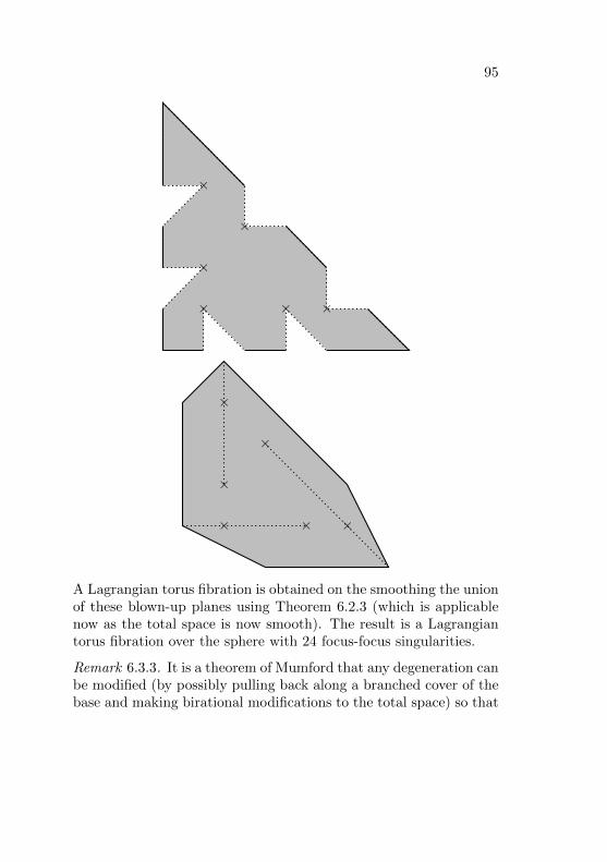
95

× ×

×

×

×

×

× ×

×

×

×

×

A Lagrangian torus fibration is obtained on the smoothing the unionof these blown-up planes using Theorem 6.2.3 (which is applicablenow as the total space is now smooth). The result is a Lagrangiantorus fibration over the sphere with 24 focus-focus singularities.

Remark 6.3.3. It is a theorem of Mumford that any degeneration canbe modified (by possibly pulling back along a branched cover of thebase and making birational modifications to the total space) so that

96 6.4. Exercises

the total space is smooth and the singular fibre is a reduced normalcrossing variety. The local model from Theorem 6.2.3 applies in thiscase provided we can find suitable Lagrangian torus fibrations onthe irreducible components.

6.4 Exercises

Exercise 6.4.1. Consider the degeneration π : C2 → C, π(z1, z2) =z1z2, and let Ω = dx1 ∧ dy1 + dx2 ∧ dy2 (with zk = xk + iyk). Checkthat the horizontal lift (for the canonical symplectic connection) of

the vector v ∈ C at (z1, z2) is v = v|z|2

(z2

z1

)where |z|2 = |z1|2 +

|z2|2. Let γ(t) = e2πit be a parametrisation of the unit circle in Cand write z1(t) = r(t)eiθ(t), z2(t) = e2πit−θ(t)/r for the path tracedout by (z1(0), z2(0)) under symplectic parallel transport. Show thatr = 0 and θ = 1

r4+1 . Hence find the parallel transport at time 1.Plot the image of the line θ = 0 under the parallel transport map.You just showed that the time 1 parallel transport is a Dehn twist.

Exercise 6.4.2. Show that the map H : C3 → R3, H(x, y, z) =(12 (|x|2 − |y|2), 1

2 (|x|2 − |z|2), 12 |xyz − c|

)is a Lagrangian torus fi-

bration. What are the singular fibres? Show that the set of singularfibres forms a Y-graph in R3.

Bibliography

[1] V. I. Arnol’d. Mathematical methods of classical mechanics,volume 60 of Graduate Texts in Mathematics. Springer-Verlag,New York, 1989. Translated from the 1974 Russian original byK. Vogtmann and A. Weinstein, second edition.

[2] D. Auroux. Mirror symmetry and T -duality in the complementof an anticanonical divisor. J. Gokova Geom. Topol. GGT, 1:51–91, 2007.

[3] M. Chaperon. Normalisation of the smooth focus-focus: a sim-ple proof. Acta Math. Vietnam., 38(1):3–9, 2013.

[4] J.-P. Dufour and P. Molino. Compactification d’actions deRn et variables action-angle avec singularites. In Travaux duSeminaire Sud-Rhodanien de Geometrie, I, volume 88 of Publ.Dep. Math. Nouvelle Ser. B, pages 161–183. Univ. Claude-Bernard, Lyon, 1988.

[5] J. J. Duistermaat. On global action-angle coordinates. Comm.Pure Appl. Math., 33(6):687–706, 1980.

[6] L. H. Eliasson. Normal forms for Hamiltonian systems withPoisson commuting integrals—elliptic case. Comment. Math.Helv., 65(1):4–35, 1990.

97

98 BIBLIOGRAPHY

[7] J. Kollar and N. I. Shepherd-Barron. Threefolds and defor-mations of surface singularities. Invent. Math., 91(2):299–338,1988.

[8] R. Schoen and J. Wolfson. Minimizing area among Lagrangiansurfaces: the mapping problem. J. Differential Geom., 58(1):1–86, 2001.

[9] D. Sepe and S. Vu Ngo.c. Integrable systems, symmetries, andquantization. Lett. Math. Phys., 108(3):499–571, 2018.

[10] M. Symington. Four dimensions from two in symplectic topol-ogy. In Topology and geometry of manifolds (Athens, GA,2001), volume 71 of Proc. Sympos. Pure Math., pages 153–208.Amer. Math. Soc., Providence, RI, 2003.

[11] S. Vu Ngo.c. On semi-global invariants for focus-focus singular-ities. Topology, 42(2):365–380, 2003.