Lagrangian Relaxation of Magnetic Fields
20
Lagrangian Relaxation of Magnetic Fields Simon Candelaresi
-
Upload
simon-candelaresi -
Category
Science
-
view
35 -
download
0
Transcript of Lagrangian Relaxation of Magnetic Fields
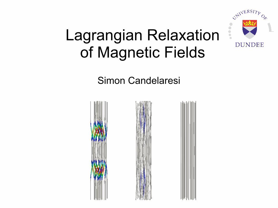
Lagrangian Relaxationof Magnetic Fields
Simon Candelaresi

2
Force-Free Magnetic Fields
NASA
Solar corona: low plasma beta and magnetic resistivity
Force-free magnetic fields
Problem:Find a force-free state for a magnetic field with given topology.
Beltrami field
Minimum energy state
Here:Numerical method for finding such states.
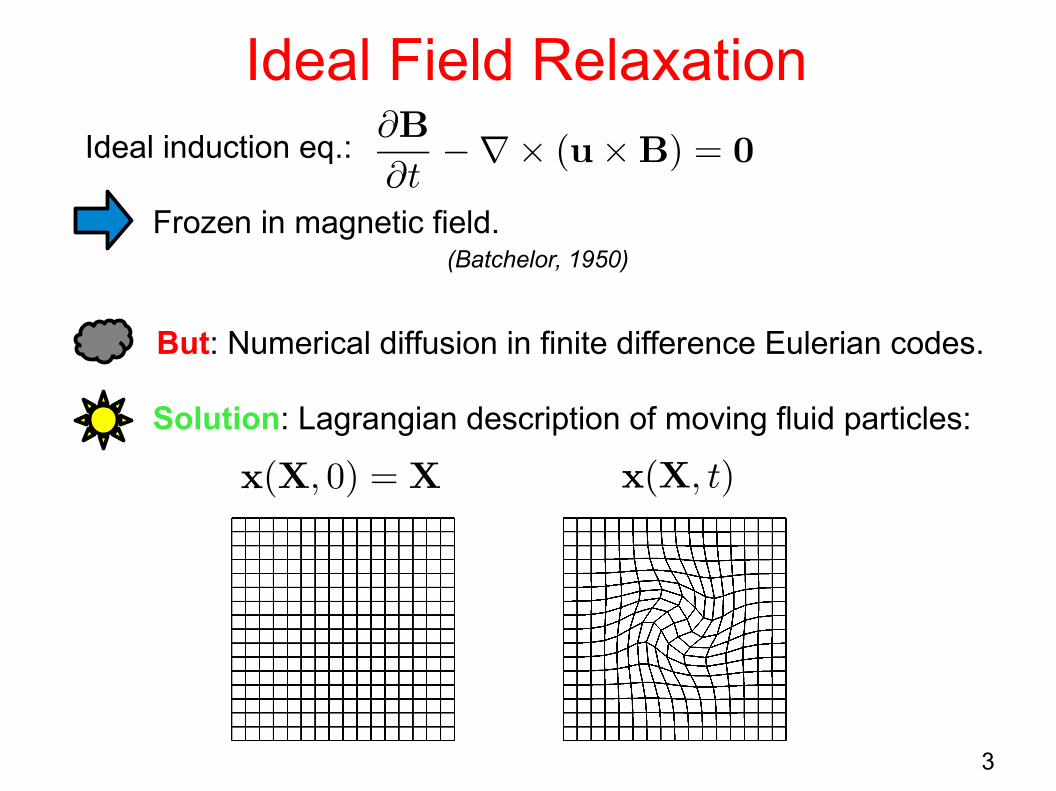
Ideal induction eq.:
Solution: Lagrangian description of moving fluid particles:
3
Ideal Field Relaxation
But: Numerical diffusion in finite difference Eulerian codes.
Frozen in magnetic field.(Batchelor, 1950)

4
Ideal Field Relaxation
Magneto-frictional term:
Field evolution:
Preserves topology and divergence-freeness.
(Craig and Sneyd 1986)
Grid evolution:

5
Numerical Curl Operator
Compute on a distorted grid:
Multiplication of several terms leads to high numerical errors.
Only reaching a certain force-freeness.
Current not divergence free:
(Craig and Sneyd 1986)
(Pontin et al. 2009)
6
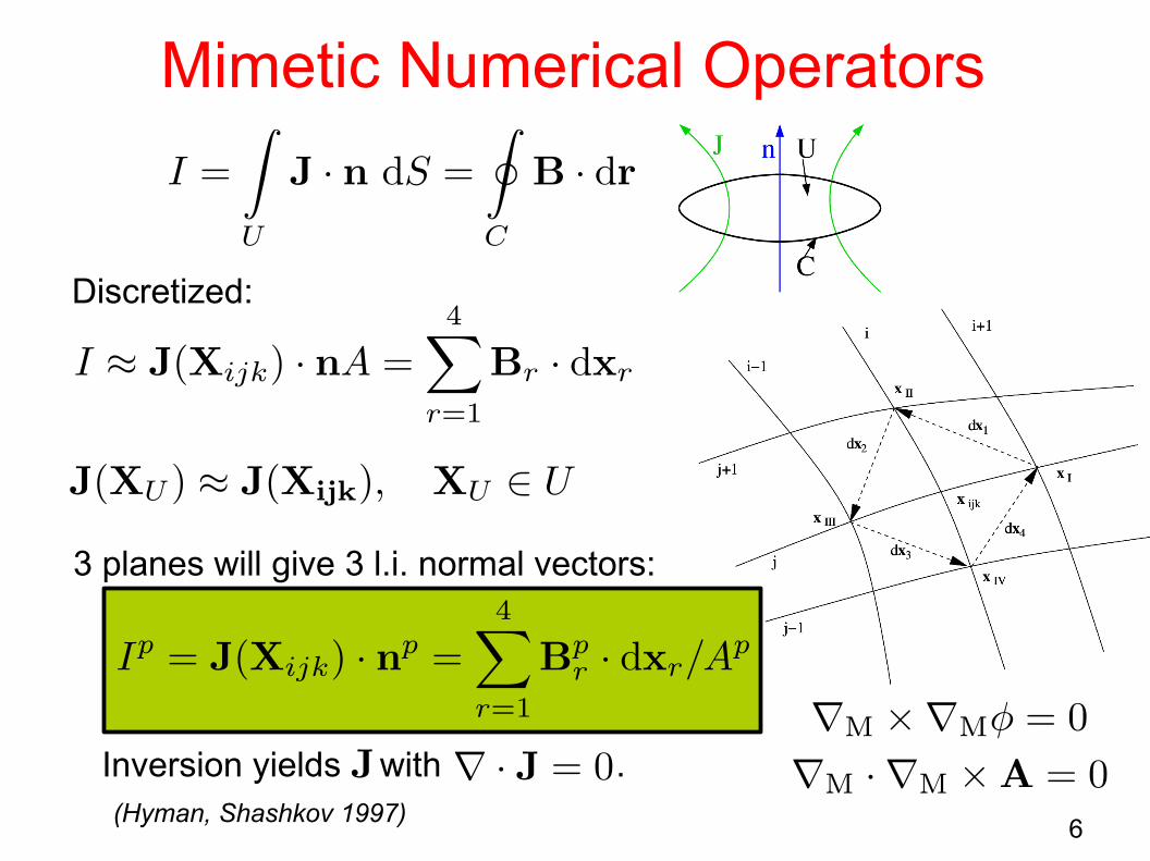
Mimetic Numerical Operators
Discretized:
3 planes will give 3 l.i. normal vectors:
Inversion yields with .(Hyman, Shashkov 1997)
7
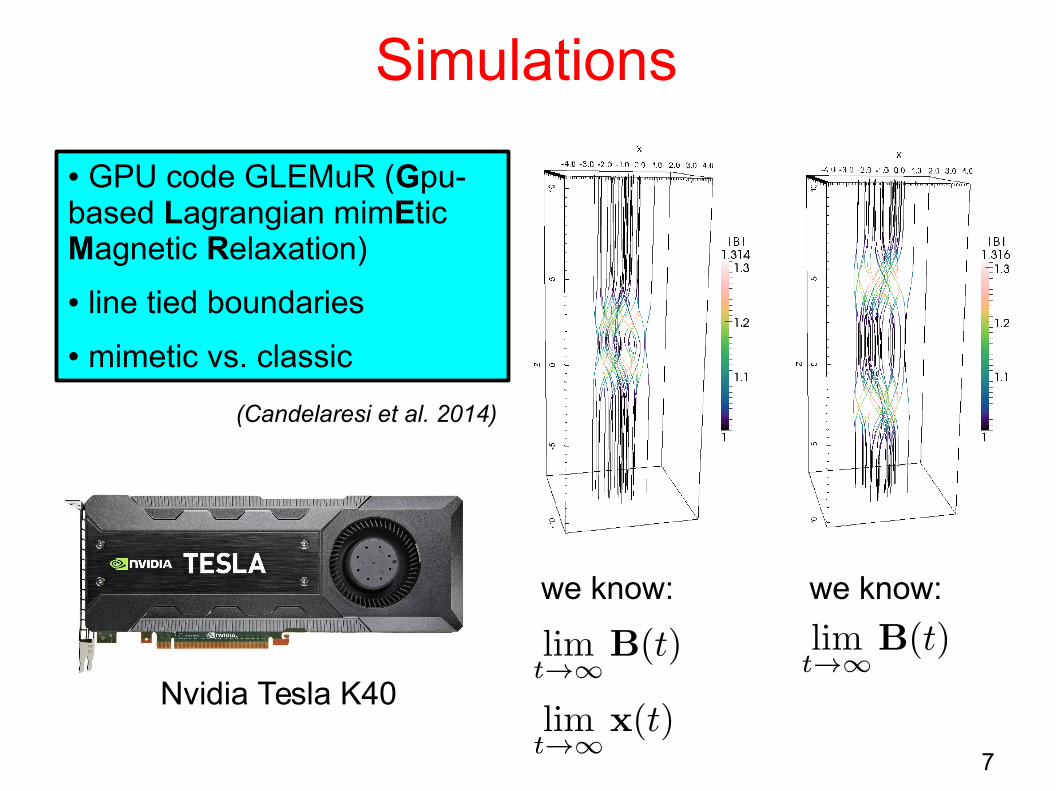
Simulations
we know: we know:
● GPU code GLEMuR (Gpu-based Lagrangian mimEtic Magnetic Relaxation)
● line tied boundaries
● mimetic vs. classic
Nvidia Tesla K40
(Candelaresi et al. 2014)

Deviation from the expected relaxed state:
8
Quality Parameters
Free magnetic energy:
9
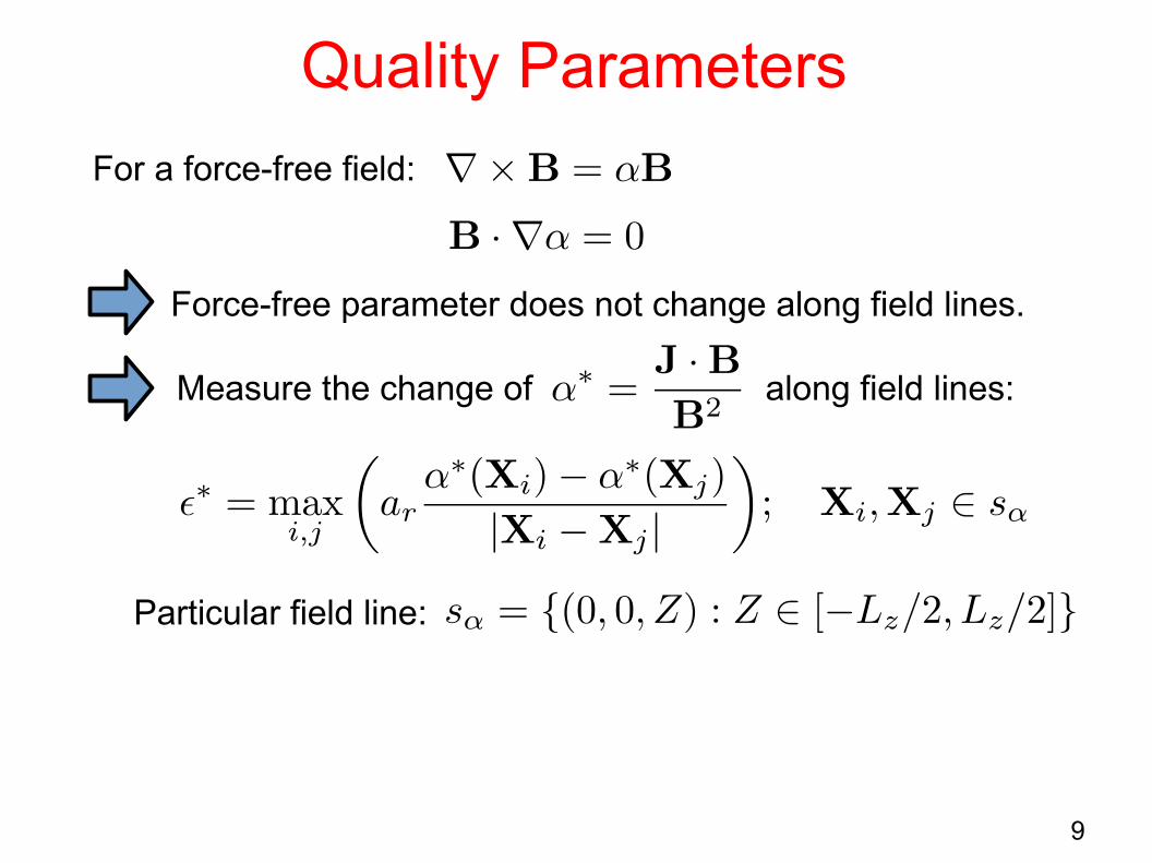
For a force-free field:
Force-free parameter does not change along field lines.
Quality Parameters
Measure the change of along field lines:
Particular field line:

10
Field Relaxation
movie
Magnetic streamlines: Grid distortion at mid-plane:
11
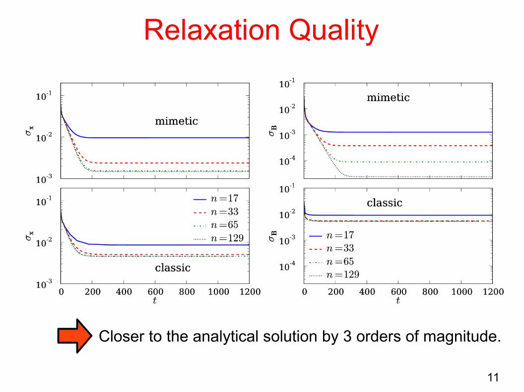
Relaxation Quality
Closer to the analytical solution by 3 orders of magnitude.

12
Relaxation Quality
Closer to force-free state by 5 orders of magnitude.
13
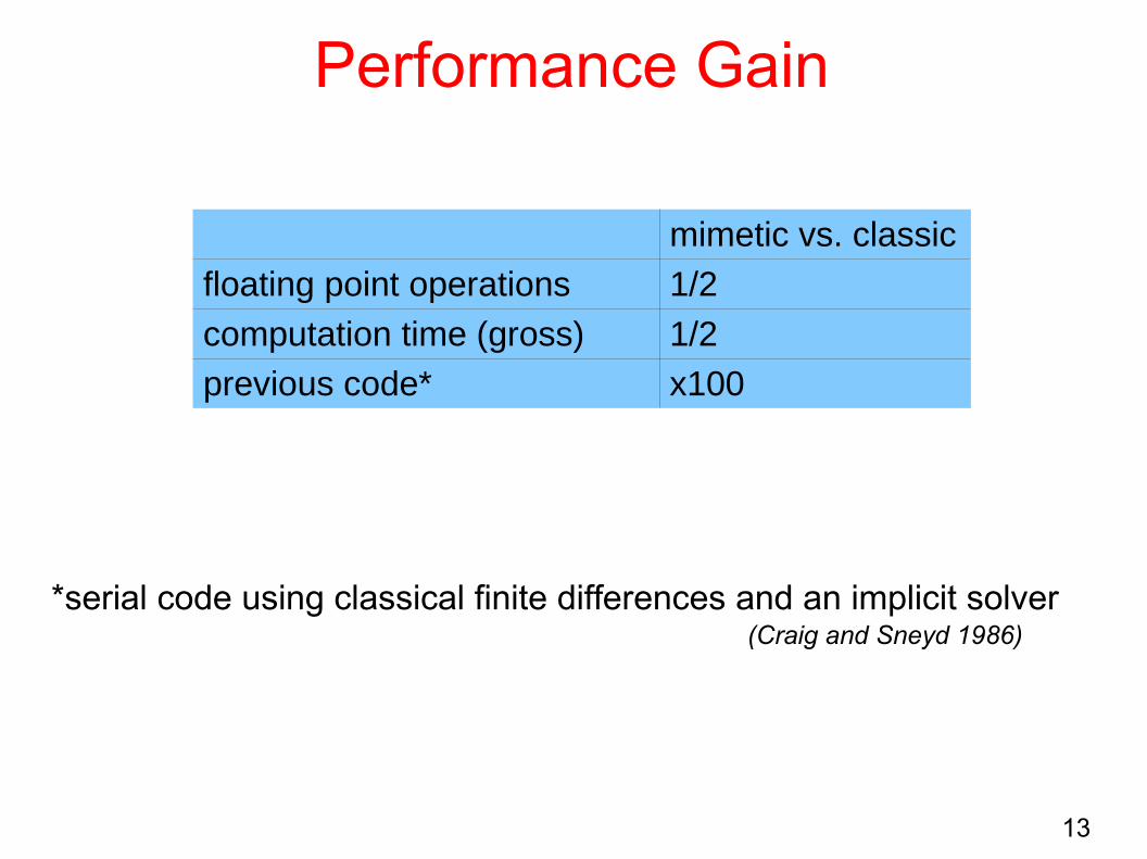
Performance Gain
mimetic vs. classic
floating point operations 1/2
computation time (gross) 1/2
previous code* x100
*serial code using classical finite differences and an implicit solver(Craig and Sneyd 1986)

14
Limitations
red: convexblue: concave
For concave cells the method becomes unstable.But: results before crash better than classic method.
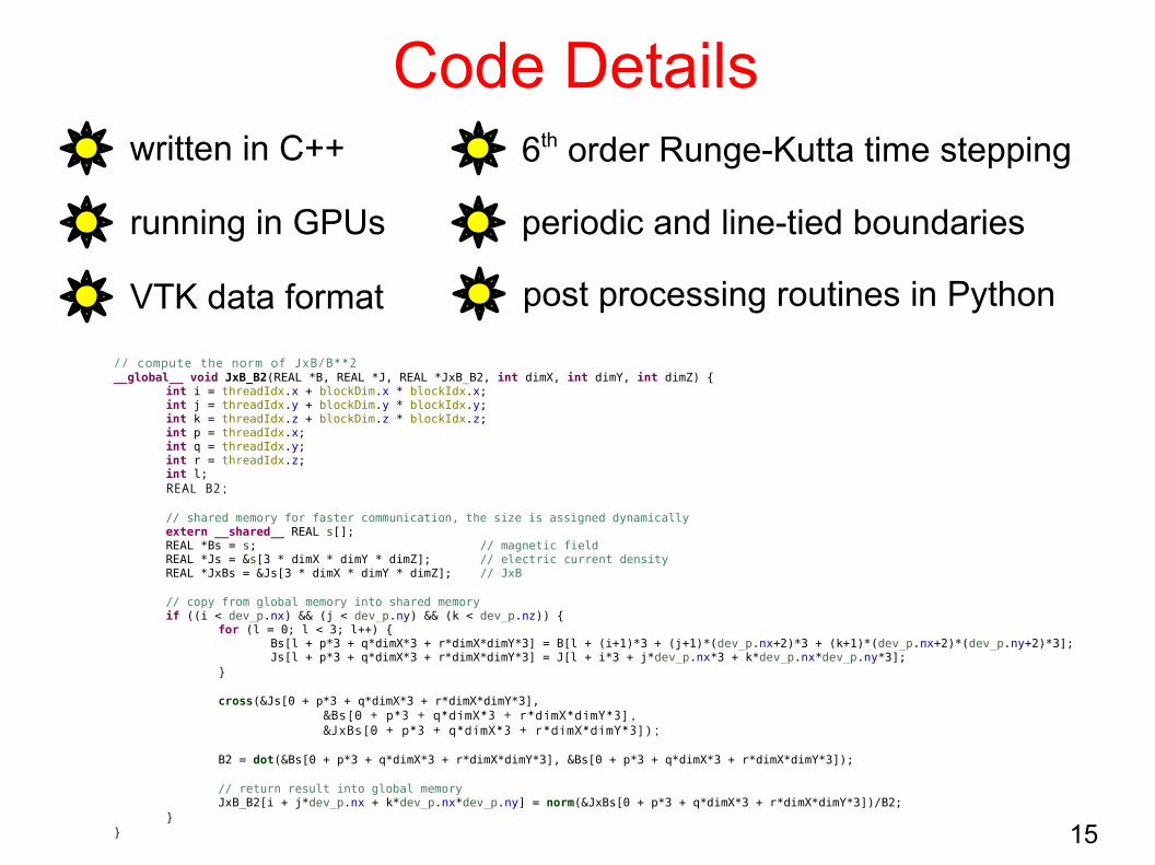
Code Details
15
// compute the norm of JxB/B**2__global__ void JxB_B2(REAL *B, REAL *J, REAL *JxB_B2, int dimX, int dimY, int dimZ) {
int i = threadIdx.x + blockDim.x * blockIdx.x;int j = threadIdx.y + blockDim.y * blockIdx.y;int k = threadIdx.z + blockDim.z * blockIdx.z;int p = threadIdx.x;int q = threadIdx.y;int r = threadIdx.z;int l;REAL B2;
// shared memory for faster communication, the size is assigned dynamicallyextern __shared__ REAL s[];REAL *Bs = s; // magnetic fieldREAL *Js = &s[3 * dimX * dimY * dimZ]; // electric current densityREAL *JxBs = &Js[3 * dimX * dimY * dimZ]; // JxB
// copy from global memory into shared memoryif ((i < dev_p.nx) && (j < dev_p.ny) && (k < dev_p.nz)) {
for (l = 0; l < 3; l++) {Bs[l + p*3 + q*dimX*3 + r*dimX*dimY*3] = B[l + (i+1)*3 + (j+1)*(dev_p.nx+2)*3 + (k+1)*(dev_p.nx+2)*(dev_p.ny+2)*3];Js[l + p*3 + q*dimX*3 + r*dimX*dimY*3] = J[l + i*3 + j*dev_p.nx*3 + k*dev_p.nx*dev_p.ny*3];
}
cross(&Js[0 + p*3 + q*dimX*3 + r*dimX*dimY*3],&Bs[0 + p*3 + q*dimX*3 + r*dimX*dimY*3],&JxBs[0 + p*3 + q*dimX*3 + r*dimX*dimY*3]);
B2 = dot(&Bs[0 + p*3 + q*dimX*3 + r*dimX*dimY*3], &Bs[0 + p*3 + q*dimX*3 + r*dimX*dimY*3]);
// return result into global memoryJxB_B2[i + j*dev_p.nx + k*dev_p.nx*dev_p.ny] = norm(&JxBs[0 + p*3 + q*dimX*3 + r*dimX*dimY*3])/B2;
}}
written in C++
running in GPUs
6th order Runge-Kutta time stepping
VTK data format post processing routines in Python
periodic and line-tied boundaries

16
GLEMuR vs. PencilCode
GLEMuR PencilCode
data format VTK PC
language C++ Fortran
change # cores
compile once
post processing Python IDL/Python
bash tools
GPU
CPU
general MHD

Similarities with the PencilCode
17
time_series.dat
Fortran name lists&comp nx = 33; ny = 33; nz = 33/
&start Lx = 0.6; Ly = 0.6; Lz = 1.0 Ox = -0.3; Oy = -0.3; Oz = -0.5 bInit = "sheared" ampl = 1. initDist = "initShearX" initShear0 = 0.7 initShearK = 1. fRestart = t/
# it t dt maxDelta JxB_B2Max epsilonStar B2 convex 0 1.29540e-06 1.29540e-06 1.78814e-07 1.50932e+02 2.81160e+02 7.12394e-01 -1.00000e+00 1 3.08508e-06 1.78967e-06 1.19209e-07 1.13175e+02 2.96738e+02 7.12170e-01 -1.00000e+00 2 5.76647e-06 2.68139e-06 1.78814e-07 8.83429e+01 3.15884e+02 7.11882e-01 -1.00000e+00 3 9.47096e-06 3.70449e-06 1.19209e-07 7.67879e+01 3.36120e+02 7.11536e-01 -1.00000e+00 4 1.50212e-05 5.55028e-06 1.78814e-07 6.44194e+01 3.57402e+02 7.11085e-01 -1.00000e+00 5 2.13638e-05 6.34253e-06 7.74860e-07 5.44002e+01 3.73753e+02 7.10636e-01 -1.00000e+00
gm_ci_run gm_inspectrun gm_newrun
Bash commands
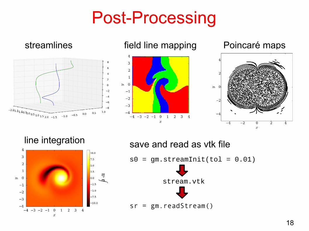
Post-Processing
18
streamlines Poincaré maps
line integration save and read as vtk file
field line mapping
sr = gm.readStream()
s0 = gm.streamInit(tol = 0.01)
stream.vtk
Outlook
19
● GLEMuR to PC data conversion
● More physics (multi purpose)
● Run on GPU clusters
● PencilCode on GPUs?
Conclusions
● Lagrangian numerical scheme for ideal evolution.
● Preserving field line topology.
● Mimetic methods more capable of producing force-free fields.
● GLEMuR code running on GPUs.
● Performance gain of x2 compared to classical approach.
● GLEMuR vs. PencilCode
● Design features from the PencilCode