Laffont & Martimort - The Theory of Incentives.pdf
381
THE THEORY OF INCENTIVES I : THE PRINCIPAL-AGENT MODEL Jean-Jacques Laffont & David Martimort February 6, 2001
Transcript of Laffont & Martimort - The Theory of Incentives.pdf

THE THEORY OF INCENTIVES I :THE PRINCIPAL-AGENT MODEL
Jean-Jacques Laffont & David Martimort
February 6, 2001

2
Contents
1 Incentives in Economic Thought 17
1.1 Introduction . . . . . . . . . . . . . . . . . . . . . . . . . . . . . . . . . . . 17
1.2 Adam Smith and Incentive Contracts in Agriculture . . . . . . . . . . . . . 18
1.3 Chester Barnard and Incentives in Management . . . . . . . . . . . . . . . 20
1.4 Hume, Wicksell, Groves: The Free Rider Problem . . . . . . . . . . . . . . 23
1.5 Borda, Bowen, Vickrey: Incentives in Voting . . . . . . . . . . . . . . . . . 25
1.6 Leon Walras and the Regulation of Natural Monopolies . . . . . . . . . . . 27
1.7 Knight, Arrow, Pauly: Incentives in Insurance . . . . . . . . . . . . . . . . 28
1.8 Sidgwick, Vickrey, Mirrlees: Redistribution and Incentives . . . . . . . . . 29
1.9 Dupuit, Edgeworth, Pigou: Price Discrimination . . . . . . . . . . . . . . . 31
1.10 Incentives in Planned Economies . . . . . . . . . . . . . . . . . . . . . . . 32
1.11 Leonid Hurwicz and Mechanism Design . . . . . . . . . . . . . . . . . . . . 34
1.12 Auctions . . . . . . . . . . . . . . . . . . . . . . . . . . . . . . . . . . . . . 36
2 The Rent Extraction-Efficiency Trade-Off 37
2.1 Introduction . . . . . . . . . . . . . . . . . . . . . . . . . . . . . . . . . . . 37
2.2 The Basic Model . . . . . . . . . . . . . . . . . . . . . . . . . . . . . . . . 40
2.2.1 Technology, Preferences and Information . . . . . . . . . . . . . . . 40
2.2.2 Contracting Variables . . . . . . . . . . . . . . . . . . . . . . . . . . 41
2.2.3 Timing . . . . . . . . . . . . . . . . . . . . . . . . . . . . . . . . . . 41
2.3 The Complete Information Optimal Contract . . . . . . . . . . . . . . . . 41
3

4 CONTENTS
2.3.1 First-Best Production Levels . . . . . . . . . . . . . . . . . . . . . . 41
2.3.2 Implementation of the First-Best . . . . . . . . . . . . . . . . . . . 42
2.3.3 A Graphical Representation of the Complete Information Optimal
Contract . . . . . . . . . . . . . . . . . . . . . . . . . . . . . . . . . 43
2.4 Incentive Feasible Menu of Contracts . . . . . . . . . . . . . . . . . . . . . 44
2.4.1 Incentive Compatibility and Participation . . . . . . . . . . . . . . 44
2.4.2 Special Cases . . . . . . . . . . . . . . . . . . . . . . . . . . . . . . 46
2.4.3 Monotonicity Constraints . . . . . . . . . . . . . . . . . . . . . . . 46
2.5 Information Rents . . . . . . . . . . . . . . . . . . . . . . . . . . . . . . . . 47
2.6 The Optimization Program of the Principal . . . . . . . . . . . . . . . . . 48
2.7 The Rent Extraction-Efficiency Trade-Off . . . . . . . . . . . . . . . . . . . 49
2.7.1 The Asymmetric Information Optimal Contract . . . . . . . . . . . 49
2.7.2 A Graphical Representation of the Second-Best Outcome . . . . . . 51
2.7.3 Shut-Down Policy . . . . . . . . . . . . . . . . . . . . . . . . . . . . 53
2.8 The Theory of the Firm under Asymmetric Information . . . . . . . . . . . 54
2.9 Asymmetric Information and Marginal Cost Pricing . . . . . . . . . . . . . 55
2.10 The Revelation Principle . . . . . . . . . . . . . . . . . . . . . . . . . . . . 56
2.11 A More General Utility Function for the Agent . . . . . . . . . . . . . . . . 58
2.11.1 The Optimal Contract . . . . . . . . . . . . . . . . . . . . . . . . . 59
2.11.2 Non-Responsiveness . . . . . . . . . . . . . . . . . . . . . . . . . . . 61
2.11.3 More Than Two Goods . . . . . . . . . . . . . . . . . . . . . . . . . 63
2.12 Ex Ante Versus Ex Post Participation Constraints . . . . . . . . . . . . . . 64
2.12.1 Risk Neutrality . . . . . . . . . . . . . . . . . . . . . . . . . . . . . 64
2.12.2 Risk Aversion . . . . . . . . . . . . . . . . . . . . . . . . . . . . . . 66
2.13 Commitment . . . . . . . . . . . . . . . . . . . . . . . . . . . . . . . . . . 70
2.13.1 Renegotiating a Contract . . . . . . . . . . . . . . . . . . . . . . . . 70
2.13.2 Reneging on a Contract . . . . . . . . . . . . . . . . . . . . . . . . 71
2.14 Stochastic Mechanisms . . . . . . . . . . . . . . . . . . . . . . . . . . . . . 71

CONTENTS 5
2.15 Informative Signals to Improve Contracting . . . . . . . . . . . . . . . . . 75
2.15.1 Ex Post Verifiable Signal . . . . . . . . . . . . . . . . . . . . . . . . 75
2.15.2 Ex Ante Nonverifiable Signal . . . . . . . . . . . . . . . . . . . . . . 76
2.15.3 More or Less Favorable Distribution of Types . . . . . . . . . . . . 77
2.16 Contract Theory at Work . . . . . . . . . . . . . . . . . . . . . . . . . . . 78
2.16.1 Regulation . . . . . . . . . . . . . . . . . . . . . . . . . . . . . . . . 78
2.16.2 Nonlinear Pricing of a Monopoly . . . . . . . . . . . . . . . . . . . 79
2.16.3 Quality and Price Discrimination . . . . . . . . . . . . . . . . . . . 80
2.16.4 Financial Contracts . . . . . . . . . . . . . . . . . . . . . . . . . . . 81
2.16.5 Labor Contracts . . . . . . . . . . . . . . . . . . . . . . . . . . . . . 82
3 Incentive and Participation Constraints 91
3.1 Introduction . . . . . . . . . . . . . . . . . . . . . . . . . . . . . . . . . . . 91
3.2 More than Two Types . . . . . . . . . . . . . . . . . . . . . . . . . . . . . 94
3.2.1 Incentive Feasible Contracts . . . . . . . . . . . . . . . . . . . . . . 94
3.2.2 The Optimal Contract . . . . . . . . . . . . . . . . . . . . . . . . . 96
3.2.3 The Spence-Mirrlees Condition . . . . . . . . . . . . . . . . . . . . 98
3.3 Multi-dimensional Asymmetric Information . . . . . . . . . . . . . . . . . . 100
3.3.1 A Discrete Model . . . . . . . . . . . . . . . . . . . . . . . . . . . . 100
3.3.2 The Optimal Contract . . . . . . . . . . . . . . . . . . . . . . . . . 102
3.3.3 Continuum of Types . . . . . . . . . . . . . . . . . . . . . . . . . . 107
3.4 State Dependent . . . . . . . . . . . . . . . . . . . . . . . . . . . . . . . . 108
3.4.1 The Optimal Contract . . . . . . . . . . . . . . . . . . . . . . . . . 108
3.4.2 Countervailing Incentives: Examples . . . . . . . . . . . . . . . . . 112
3.5 Random Participation Constraint . . . . . . . . . . . . . . . . . . . . . . . 121
3.6 Limited Liability . . . . . . . . . . . . . . . . . . . . . . . . . . . . . . . . 124
3.7 Audit Mechanisms . . . . . . . . . . . . . . . . . . . . . . . . . . . . . . . 127
3.7.1 Incentive-Feasible Audit Mechanisms . . . . . . . . . . . . . . . . . 127

6 CONTENTS
3.7.2 Optimal Audit Mechanism . . . . . . . . . . . . . . . . . . . . . . . 129
3.7.3 Financial Contracting . . . . . . . . . . . . . . . . . . . . . . . . . 131
3.7.4 The Threat of Termination . . . . . . . . . . . . . . . . . . . . . . . 132
3.8 Redistributive Concerns . . . . . . . . . . . . . . . . . . . . . . . . . . . . 135
4 Moral Hazard: The Basic Trade-Offs 147
4.1 Introduction . . . . . . . . . . . . . . . . . . . . . . . . . . . . . . . . . . . 147
4.2 The Model . . . . . . . . . . . . . . . . . . . . . . . . . . . . . . . . . . . . 150
4.2.1 Effort and Production . . . . . . . . . . . . . . . . . . . . . . . . . 150
4.2.2 Incentive Feasible Contracts . . . . . . . . . . . . . . . . . . . . . . 151
4.2.3 The Complete Information Optimal Contract . . . . . . . . . . . . 153
4.3 Risk Neutrality and First-Best Implementation . . . . . . . . . . . . . . . . 154
4.4 The Trade-Off between Limited Liability . . . . . . . . . . . . . . . . . . . 156
4.5 The Trade-Off Between Insurance and Efficiency . . . . . . . . . . . . . . . 159
4.5.1 Optimal Transfers . . . . . . . . . . . . . . . . . . . . . . . . . . . . 160
4.5.2 Optimal Second-Best Effort . . . . . . . . . . . . . . . . . . . . . . 161
4.6 More Than Two Levels of Performance . . . . . . . . . . . . . . . . . . . . 163
4.6.1 Limited Liability . . . . . . . . . . . . . . . . . . . . . . . . . . . . 163
4.6.2 Risk Aversion . . . . . . . . . . . . . . . . . . . . . . . . . . . . . . 165
4.7 Informative Signals to Improve Contracting . . . . . . . . . . . . . . . . . 167
4.7.1 Informativeness of Signals . . . . . . . . . . . . . . . . . . . . . . . 167
4.7.2 More Comparisons among Information Structures . . . . . . . . . . 169
4.8 Moral Hazard and the Theory of the Firm . . . . . . . . . . . . . . . . . . 171
4.9 Contract Theory at Work . . . . . . . . . . . . . . . . . . . . . . . . . . . 171
4.9.1 Efficiency Wage . . . . . . . . . . . . . . . . . . . . . . . . . . . . . 171
4.9.2 Sharecropping . . . . . . . . . . . . . . . . . . . . . . . . . . . . . . 172
4.9.3 Wholesale Contracts . . . . . . . . . . . . . . . . . . . . . . . . . . 174
4.9.4 Financial Contracts . . . . . . . . . . . . . . . . . . . . . . . . . . . 174

CONTENTS 7
4.9.5 Insurance Contract . . . . . . . . . . . . . . . . . . . . . . . . . . . 177
4.10 Commitment under Moral Hazard . . . . . . . . . . . . . . . . . . . . . . . 180
5 Incentive and Participation Contraints 183
5.1 Introduction . . . . . . . . . . . . . . . . . . . . . . . . . . . . . . . . . . . 183
5.2 More Than Two Levels of Effort . . . . . . . . . . . . . . . . . . . . . . . . 187
5.2.1 A Discrete Model . . . . . . . . . . . . . . . . . . . . . . . . . . . . 187
5.2.2 Two Outcomes with a Continuum of Effort Levels . . . . . . . . . . 190
5.2.3 The “first-order Approach” . . . . . . . . . . . . . . . . . . . . . . 191
5.3 The Multi-Task Incentive Problem . . . . . . . . . . . . . . . . . . . . . . 196
5.3.1 Technology . . . . . . . . . . . . . . . . . . . . . . . . . . . . . . . 196
5.3.2 The Simple Case of Limited Liability . . . . . . . . . . . . . . . . . 197
5.3.3 The Optimal Contract for a Risk Averse Agent . . . . . . . . . . . 202
5.3.4 Asymmetric Tasks . . . . . . . . . . . . . . . . . . . . . . . . . . . 208
5.3.5 Applications of the Multi-Task Framework . . . . . . . . . . . . . . 211
5.4 Nonseparability in the Utility Function . . . . . . . . . . . . . . . . . . . . 219
5.4.1 Non-Binding Participation Constraint . . . . . . . . . . . . . . . . . 219
5.4.2 A Specific Model with no Wealth Effect . . . . . . . . . . . . . . . . 222
5.5 Redistribution and Moral Hazard . . . . . . . . . . . . . . . . . . . . . . . 224
6 Non-verifiability 231
6.1 Introduction . . . . . . . . . . . . . . . . . . . . . . . . . . . . . . . . . . . 231
6.2 No Contract at Date 0 and Ex Post Bargaining . . . . . . . . . . . . . . . 233
6.3 Incentive Compatible Contract . . . . . . . . . . . . . . . . . . . . . . . . . 234
6.4 Nash Implementation . . . . . . . . . . . . . . . . . . . . . . . . . . . . . . 236
6.5 Subgame Perfect Implementation . . . . . . . . . . . . . . . . . . . . . . . 246
6.6 Risk Aversion . . . . . . . . . . . . . . . . . . . . . . . . . . . . . . . . . . 251
6.6.1 Risk Averse Agent . . . . . . . . . . . . . . . . . . . . . . . . . . . 251
6.6.2 Risk Averse Principal . . . . . . . . . . . . . . . . . . . . . . . . . . 251
8 CONTENTS
6.7 Concluding Remarks . . . . . . . . . . . . . . . . . . . . . . . . . . . . . . 253
7 Mixed Models 255
7.1 Introduction . . . . . . . . . . . . . . . . . . . . . . . . . . . . . . . . . . . 255
7.2 Adverse Selection Followed by Moral Hazard . . . . . . . . . . . . . . . . . 258
7.2.1 Random Surplus and Screening . . . . . . . . . . . . . . . . . . . . 258
7.2.2 The Extended Revelation Principle . . . . . . . . . . . . . . . . . . 263
7.2.3 Insurance Contracts with Adverse Selection . . . . . . . . . . . . . 265
7.2.4 Models with “False Moral Hazard” . . . . . . . . . . . . . . . . . . 274
7.3 Moral Hazard Followed by Adverse Selection . . . . . . . . . . . . . . . . . 280
7.3.1 The Model . . . . . . . . . . . . . . . . . . . . . . . . . . . . . . . . 281
7.3.2 The Case of Risk Neutrality . . . . . . . . . . . . . . . . . . . . . . 282
7.3.3 Limited Liability and Output Inefficiency . . . . . . . . . . . . . . . 283
7.4 Moral Hazard Followed by Non-verifiability . . . . . . . . . . . . . . . . . . 285
8 Dynamics Under Full Commitment 289
8.1 Introduction . . . . . . . . . . . . . . . . . . . . . . . . . . . . . . . . . . . 289
8.2 Adverse Selection . . . . . . . . . . . . . . . . . . . . . . . . . . . . . . . . 292
8.2.1 Perfect Correlation of Types . . . . . . . . . . . . . . . . . . . . . . 293
8.2.2 Independent Types . . . . . . . . . . . . . . . . . . . . . . . . . . . 296
8.2.3 Correlated Types . . . . . . . . . . . . . . . . . . . . . . . . . . . . 297
8.3 A Digression on Non-Commitment . . . . . . . . . . . . . . . . . . . . . . 301
8.4 Moral Hazard . . . . . . . . . . . . . . . . . . . . . . . . . . . . . . . . . . 301
8.4.1 The Model . . . . . . . . . . . . . . . . . . . . . . . . . . . . . . . . 301
8.4.2 The Optimal Long-Term Contract . . . . . . . . . . . . . . . . . . . 302
8.4.3 Renegotiation-Proofness . . . . . . . . . . . . . . . . . . . . . . . . 307
8.4.4 Reneging on the Contract . . . . . . . . . . . . . . . . . . . . . . . 308
8.4.5 Saving . . . . . . . . . . . . . . . . . . . . . . . . . . . . . . . . . . 310
8.4.6 Infinitely Repeated Relationship . . . . . . . . . . . . . . . . . . . . 313

CONTENTS 9
8.5 Application: The Dynamics of Insurance Contracts . . . . . . . . . . . . . 319
9 Limits and Extensions 321
9.1 Introduction . . . . . . . . . . . . . . . . . . . . . . . . . . . . . . . . . . . 321
9.2 Informed Principal . . . . . . . . . . . . . . . . . . . . . . . . . . . . . . . 324
9.3 Limits to Enforcement . . . . . . . . . . . . . . . . . . . . . . . . . . . . . 334
9.4 Dynamics and Limited Commitment . . . . . . . . . . . . . . . . . . . . . 338
9.5 The Hold-Up Problem . . . . . . . . . . . . . . . . . . . . . . . . . . . . . 343
9.5.1 Adverse Selection . . . . . . . . . . . . . . . . . . . . . . . . . . . . 343
9.5.2 Non-verifiability . . . . . . . . . . . . . . . . . . . . . . . . . . . . . 344
9.6 Limits to the Complexity of Contracts . . . . . . . . . . . . . . . . . . . . 346
9.6.1 Menu of Linear Contracts under Adverse Selection . . . . . . . . . . 346
9.6.2 Linear Sharing Rules and Moral Hazard . . . . . . . . . . . . . . . 350
9.7 Limits in the Action Space . . . . . . . . . . . . . . . . . . . . . . . . . . . 355
9.7.1 Extending the Action Space . . . . . . . . . . . . . . . . . . . . . . 355
9.7.2 Costly Action Space . . . . . . . . . . . . . . . . . . . . . . . . . . 357
9.8 Limits to Rational Behavior . . . . . . . . . . . . . . . . . . . . . . . . . . 359
9.8.1 Trembling-Hand Behavior . . . . . . . . . . . . . . . . . . . . . . . 359
9.8.2 Satisficing Behavior . . . . . . . . . . . . . . . . . . . . . . . . . . . 361
9.8.3 Costly Communication and Complexity . . . . . . . . . . . . . . . . 362
9.9 Endogenous Information Structures . . . . . . . . . . . . . . . . . . . . . . 362

“As the economy of incentives as a whole in terms of organization is not
usually stressed in economic theory and is certainly not well understood, I
shall attempt to indicate the outlines of the theory.”
Chester Barnard (1938)

Introduction
It is surprising to observe that Schumpeter (1954) does not mention the word of incentives
in his monumental history of economic thought. How is it possible when today, for many
economists, economics is to a large extent a matter of incentives: Incentives to work hard,
incentive to produce good quality products, incentives to study, incentives to invest,
incentives to save,... How to design institutions in order to provide good incentives for
economic agents is a central question of economics today.
Maybe, it is because economics has mostly concentrated on understanding the theory
of value in large economies. No eclassical economics in particular postulates rational in-
dividual behavior in the market. In a perfectly competitive market, this translates for
firms’ owners into profit maximization which implies cost minimization. In order words,
the pressure of competitive markets solves the problem of incentives for cost minimization.
Similarly, consumers faced with exogenous prices have the proper incentives for maximiz-
ing their utility levels. The major project of understanding how prices are formed in
competitive markets can proceed without worrying about incentives.
However, by treating the firm as a black box, the theory remains silent on how the
owners of firms succeed in aligning the objectives of its various members like workers,
supervisors, managers with profit maximization. When economists began to look more
carefully at the firm, either in agricultural economics or in managerial economics, incen-
tives became central. Indeed, for various reasons, the owner of the firm must delegate
various tasks to the members of the firm. This raises first the problems of managing infor-
mation flows within the firm. This was the first research topic for economists, once they
mastered behavior under uncertainty, thanks to Von Neumann and Morgenstern (1943).
This line of research culminated in the theory of teams (Marschak and Radner (1972)).
This theory recognized the decentralized nature of information, but postulated identical
objective functions for the members of the firm considered as a “team”. How to coordi-
nate actions among the members of the team by the proper management of information
was the central focus of this research. Incentive questions were still outside the scope of
the analysis.
However, as soon as one acknowledges that the members of a firm may have different
11
12 CONTENTS
objectives, delegation becomes more problematic as recognized early by Marschak (1955)
and also by Arrow (1968) when he observes:
“by definition the agent has been selected for his specialized knowledge and
the principal can never hope to completely check the agent’s performance.”
Delegation of a task to an agent who has different objectives than the principal who
delegates this task is problematic when information about the agent is imperfect. This is
the essence of incentive questions. If the agent had a different objective function but no
private information, the principal could propose a contract which perfectly controls the
agent and induces the latter’s actions to be what he would like to do himself in a world
without delegation. Again, incentives issues would disappear.
Conflicting objectives and decentralized information are thus the two basic ingredients
of incentive theory. That economic agents pursue at least to some extent their private
interests is the essential paradigm for the analysis of market behavior by economists. What
is proposed by incentive theory is to maintain this major assumption in the analysis of
organizations, small numbers markets and any kind of collective decision. This paradigm
has its own limits. Social behavior, in particular in small groups, is more complex, and
norms of behavior culturally inculcated play a large role in shaping societies. However, it
would be foolish not to recognize the role of private incentives in motivating behavior in
addition to these cultural phenomena. The purpose of this book is to synthesize what we
have learned from the incentives paradigm.1
We hope that the step by step approach taken here, as well as our attempt to present
many different results in a unified framework, will help the readers not only to know about
incentive theory, but to appropriate this indispensable tool for thinking about society.
The starting point of incentive theory corresponds therefore to the problem of delega-
tion of a task to an agent with private information. This private information can be of two
types : either the agent can take an action unobserved by the principal, the case of moral
hazard or hidden action ; or the agent has some private information about its cost or val-
uation that is ignored by the principal, the case of adverse selection or hidden knowledge.
The theory studies when this private information is a problem for the principal, and what
is the optimal way for the principal to cope with it. Another type of information prob-
lem has also been raised in the literature, the case of nonverifiability where the principal
and the agent share ex post the same information but no third party and, in particular,
no Court of Justice can observe this information. One can study to which extent this
nonverifiability of some piece of information is problematic for contractual design.1How do private incentives interact with cultural norms of behavior might be the next important step
of research needed to be able to offer sensible advice on the design of institutions. It is our convictionnevertheless that for such a goal the mastering of incentive theory is a must.

CONTENTS 13
We will discover that, in general, these informational problems prevent society from
achieving the first best allocation of resources which could be possible in a world where all
information is common knowledge. The additional costs that must be incurred because
of the strategic behavior of privately informed economic agents can be viewed as one
category of the transaction costs emphasized by Williamson (1975). They do not exhaust
all possible transaction costs, but economists have been rather successful during the last
thirty years, in modeling and analyzing this type of transaction costs, providing a good
understanding of the limits put by these new costs for the allocation of resources. This
work shows that the design of proper institutions for successful economic activities is more
complex than one could have thought. This whole line of research provides also a whole
set of insights on how to proceed to take into account agents’ responses to the incentives
provided by institutions.
As the next chapter will illustrate, incentive theory was pervasive in many areas of
economics, even though it was not central in economic thinking. Before describing how we
will proceed to present this theory, it may be worth mentioning how the major achievement
of economics, namely the general equilibrium theory, met incentives.
General equilibrium theory proved apt to powerful generalizations and able to deal
with uncertainty, time, externalities, extending the validity of the invisible-hand as long
as the appropriate competitive markets could be set up. However, at the beginning of
the seventies, works by Akerlof (1970), Spence (1974), and Rothschild and Stiglitz (1976)
showed in various ways that asymmetric information was posing a much greater challenge,
and could not satisfactorily be imbedded in a proper generalization of the Arrow-Debreu
theory. The problems encountered were so serious that a whole generation of general
equilibrium theorists gave up momentarily the grandiose framework of GE to reconsider
the problem of exchange under asymmetric information in its simplest form, i.e., between
two traders, and in a sense go back to basics. They joined another group trained in game
theory and in the theory of organizations to build the theory of incentives, that we take
as encompassing contract theory, principal-agent theory, agency theory and mechanism
design.
We will present incentive theory in three progressive steps. Volume I is the first step,
in which we consider the principal-agent model where the principal delegates an action
to a single agent through a take-it-or-leave-it offer of a contract.
Two implicit assumptions are made here. First, by postulating that it is the principal
who makes a-take-it-or-leave-it contract offer to the agent, we put aside the bargaining
issues which is a topic for game theory.2 Second, we assume also the availability of a
benevolent Court of Justice which is able to enforce the contract and to impose penalties
2See for example Osborne and Rubinstein (1993).

14 CONTENTS
if one of the contractual partners adopts a behavior which deviates from the that one
specified in the contract.3
Three types of information problems will be considered, adverse selection, moral
hazard and nonverifiability. Each of those informational problems leads to a different
paradigm and, possibly, to a different kind of agency costs. On top of the usual technologi-
cal constraints of neoclassical economics, these agency costs incorporate the informational
constraints faced by the principal at the time of designing the contract.
In this volume, we will assume that there are no restrictions on the contracts that
the principal can offer. As a consequence, the design of the principal’s optimal contract
reduces to a simple optimization problem.4 This simple focus will turn out to be already
enough to highlight the various trade-offs between allocative efficiency and the distribu-
tion of information rents arising under incomplete information. The mere existence of
informational constraints may generally prevent the principal from achieving allocative
efficiency. The main thrust of the analysis undertaken in this volume is therefore the char-
acterization of the allocative distortions that the principal finds desirable to implement
in order to mitigate the impact of informational constraints.
Volume II will be the second step of our analysis. We will consider there situations with
one principal and several agents, still without any restriction on the principal’s contracts.
Asymmetric information may not only affect the relationship between the principal and
each of his agents, but it may also plague the relationships between agents. Moreover,
pursuing the hypothesis that agents adopt an individualistic behavior, those organiza-
tional contexts require a new equilibrium concept, the Bayesian Nash equilibrium, which
describes the strategic interaction between agents under incomplete information. Three
main themes arise in this context. First, the organization may have been built to facili-
tate a joint decision between the agents. In such a context, the principal must overcome
the free-rider problems which might exist among agents when they must undertake a
collective decision. Second, the principal may attempt to benefit from the competition
between the agents to relax the informational constraints and better reduce the agents’
information rents. Auctions, tournaments, yardstick competition and supervision of an
agent by another one are all mechanisms designed by the principal with this purpose in
mind. Third, the mere attempt by the principal to use competition between agents may
also trigger their collusion against the principal. The principal must now worry not only
3Let us stress here the importance of this assumption which is apparently innocuous because, inequilibrium, no penalty is ever paid and the role of the court looks minimal in what follows. However,judges may have to be given proper incentives to enforce contracts. We rely here on the idea that inrepeated relationships the desire to maintain their reputation will provide the appropriate incentives.This implicit assumption is a little bit problematic since once could also appeal to the same reputationargument to justify that the principal-agent relationship may achieve allocative efficiency. It will berelaxed in Volume III.
4Hence, solving for the optimal contract requires only the simple tools of optimization theory.

CONTENTS 15
about individual incentives, but also about group incentives in a multi-agent organization.
Volume III will be the third step and will analyze the implications of various imperfec-
tions in the design of contracts: Informed principal, limited commitment, renegotiation,
imperfect coordination among various principals, incomplete contracting on the value of
trade. The dynamics of some of these imperfect contractual relationships call for the ex-
tensive use of another equilibrium concept: the Bayesian perfect equilibrium. Equipped
with this tool, we will be better able to describe the allocation of resources resulting from
such imperfect contractual relationships.
In Volume I, we proceed as follows. Chapter 1 gives a brief account of the history
of thought concerning incentive theory. It will show that incentives questions have been
present in many areas of economics over the last century even though it is only recently
that their importance has been recognized and that economists have undertaken a sys-
tematic treatment of these issues. Chapter 2 presents the basic rent extraction-efficiency
trade-off which arises in principal-agent models with adverse selection. Extensions of this
framework to more complex environments are discussed in Chapter 3. Chapter 4 presents
the two types of trade-offs under moral hazard: the trade-off between the liability rent
extraction and allocative efficiency and the trade-off between insurance and efficiency.
Again, extensions of this basic framework are discussed in Chapter 5. Chapter 6 consid-
ers the nonverifiability paradigm which in general does not call for economic distortions.
Mixed models with adverse selection, moral hazard and nonverifiability are the subject
of Chapter 7. The extension of principal-agent models with adverse selection and moral
hazard to dynamic contexts with full commitment is given in Chapter 8. Finally, Chapter
9 discusses a number of simple extensions of the basic framework used all over the book.

16 CONTENTS

Chapter 1
Incentives in Economic Thought
1.1 Introduction
Incentive theory emerges with the division of labor and exchange.1 The division of labor
induces the need for delegation and the first historical contracts appear probably in agri-
culture when a landlord contracts with his tenant. It is then no wonder that Adam Smith
encountered incentive problems in his discussion of sharecropping contracts (Section 1.2).
Delegation was also needed within firms, hence the importance of the topic in the theory
of organizations (Section 1.3).
For private goods, competitive markets ensure efficiency despite the decentralized
nature of the information about individuals’ tastes and firms’ technologies. Implicitly,
yardstick competition solves adverse selection problems and the fixed-price contracts as-
sociated with exogenous prices solve moral hazard problems. However, markets fail for
pure public goods and public intervention is thus needed. In this case, the mechanisms
used for those collective decisions must solve the incentive problem of acquiring the pri-
vate information that agents have about their preferences for public goods (Section 1.4).
Voting mechanisms are particular incentive mechanisms without any monetary transfers
for which the same question of strategic voting, i.e, not voting according to the true
preferences, can be raised (Section 1.5).
For private goods, increasing returns to scale create a situation of natural monopoly far
away from the world of competitive markets. When the monopoly has private information
about its cost or demand, its regulation by a regulatory commission becomes a principal-
agent problem (Section 1.6).
Exchange raises incentive issues when the commodity which is bought has a value
1Actually, one could also argue that incentive issues arise within the family if one postulates differentobjective functions for the members of the family.
17
18 CHAPTER 1. INCENTIVES IN ECONOMIC THOUGHT
unknown to the buyer but known to the seller. It is the case, in particular, in insurance
markets when the insurance company buys a risk plagued with moral hazard or adverse
selection. The insurance company faces a principal-agent problem with each insured agent,
but may nevertheless have a statistical knowledge of the distribution of risks (Section
1.7). A similar situation occurs when a government attempts to redistribute income
between wage earners of different and unknown productive abilities (Section 1.8) or when
a monopolist looks for the optimal discriminating contract to offer to a population of
consumers with heterogenous tastes for its product (Section 1.9). Of course, incentive
issues were encountered in managing socialist economies as profit incentives of managers
were suppressed by public ownership of the means of production (Section 1.10). The
idea that, in non-competitive economies, it is necessary to design mechanisms taking into
account communication and incentives constraints was further developed by theorists
dealing with non convex economies and this led to the mechanism design methodology
(Section 1.11). The mechanism design methodology provides a useful tool to understand
the allocation of resources in multi-agent frameworks when information is decentralized.
A natural field to apply this methodology is the theory of auctions. Auctions are indeed
mechanisms used by principals to benefit from the competition among several agents
(Section 1.12).
1.2 Adam Smith and Incentive Contracts in Agricul-
ture
In his discussion of the determination of wages (Chapter VII, Book I in Smith (1776)),
Adam Smith recognized the contractual nature of the relationship between the masters
and the workmen. He put forward the conflicting interests of those two players and
already recognized that the bargaining power was not evenly distributed between them,
the master having in general all the bargaining power. In the modern language of the
Theory of Incentives, the masters are principals and the workmen their agents.
“What are the common wages of labour, depends everywhere upon the con-
tract usually made between those two parties,whose interests are not the same.
The workmen desire to get as much, the masters to give as little as possible.”
p. 66
Smith also stressed one of the basic constraints that we model later on: The agent’s
participation constraint which limits what the principal can ask from the agent:
“A man must always live by his work, and his wages must at least be sufficient
to maintain him.” p. 67

1.2. ADAM SMITH AND INCENTIVE CONTRACTS IN AGRICULTURE 19
Smith did not have a vision of economic actors as long-run maximizers of utility. He
worried about the consequences of high-power incentives for short-run maximizers.
“Workmen, [ . . . ], when they are liberally paid by the piece, are very apt to
overwork themselves, and to ruin their health and constitution in a few years.”
p. 81
He stressed the lack of appropriate incentives for slaves:
“the work done by slaves, though it appears to cost only their maintenance,
is in the end the dearest of any. A person who can acquire no property, can
have no other interest but to eat as much, and to labour as little as possible.”
p. 365
To explain the survivance of such highly inefficient contracts, Adam Smith also ap-
pealed to non-economic motives:
“The pride of man makes him love to domineer, and nothing mortifies him so
much as to be obliged to condescend to persuade his inferiors.” p. 365
Smith’s most precise and famous discussion of incentives appears in Chapter II, Book
III, when he wants to explain the discouragement of agriculture in the ancient state of
Europe after the fall of the Roman Empire. He describes the status of metayers (Coloni
Partarii in Ancient Time, steel-bow tenants in Scotland):
“The proprietor furnished them with the seed, cattle and instruments of hus-
bandry. The produce was divided equally between the proprietor and the
farmer.” p. 366
However, Smith did not conclude that metayers will not exert the appropriate level of
effort to maximize social value, as modern incentive theory would claim.
“Such tenants, being free men, are capable of acquiring property, and having
a certain proportion of the produce of the land, they have a plain interest
that the whole produce would be as great as possible, in order that their own
proportion may be so.” p. 366

20 CHAPTER 1. INCENTIVES IN ECONOMIC THOUGHT
At several place in this volume, we will see the fundamental trade-off between incentive
and the distribution of the gains from trade. Clearly Smith was not aware of this trade-off.
Rather, he saw the most serious incentive problems in the absence of invesment in the
land by tenants and the unobservable misuse of instruments of husbandry provided by
the proprietor.
“It could never, however, be the interest even of this last species of cultivators
(the metayers) to lay out, in the further improvement of the land, any part of
the little stock they might save from their own share of the produce, because
the lord, who laid out nothing, was to get one-half of whatever it produced...
It might be the interest of metayer to make the land produce as much as
could be brought out of it by means of the stock furnished by the proprietor;
but it could never be in his interest to mix any part of his own with it. In
France,..., the proprietors complain that their metayers take every opportunity
of employing the master’s cattle rather in carriage than in cultivation; because
in the one case they get the whole profits for themselves, in the other they
share them with their landlords.” p. 367
Note the ambiguous “might”, which shows that Smith envisioned probably under-
effort but that he considered it as secondary compared to the under-investment effect.
However, the alternative use of cattle is a typical example of what we will call a hidden
action problem or a moral hazard problem.
Smith’s criticism of sharecropping has been the point of departure of a large litera-
ture in agricultural economics, in history of thought and in economic theory trying to
understand the characteristics of sharecropping contracts. Following A. Smith and un-
til Johnson (1950), economists have considered sharecropping to be a “practice which is
hurtful to the whole society”, an unexplained failure of the indivisible hand that should
be either discouraged by taxation or improved by appropriate sharing of variable fac-
tors.2 A better understanding of the phenomenon was only achieved when the economists
reconsidered the problem equipped with the principal-agent theory.3
1.3 Chester Barnard and Incentives in Management
As we saw above Smith (1776) already discussed the problems associated with piece-rate
contracts in the industry. Babbage (1835) made a further step by understanding the need
2See Schickele (1941) and Heady (1947).3See Stiglitz (1974).

1.3. CHESTER BARNARD AND INCENTIVES IN MANAGEMENT 21
for precise measurement of performances to set up efficient piece-rate or profit-sharing
contracts.
“It would, indeed, be of great mutual advantage to the industrious workman,
and to the mastermanufacturer in every trade, if the machines employed in it
could register the quantity of work which they perform, in the same manner as
a steam-engine does the number of strokes it makes. The introduction of such
contrivances gives a greater stimulus to honest industry than can readily be
imagined, and removes one of the sources of disagreement between parties.”
p. 297
Also, Babbage proposed various principles to remunerate labor:
“The general principles on which the proposed system is founded, are
1. That a considerable part of the wages received by each person should
depend on the profits made by the establishment; and,
2. That every person connected with it should derive more advantage from
applying any improvement he might discover than he could by any other
course.”
Babbage (1989, Vol. 8, p. 177).
However, Barnard (1938) can probably be credited of the first attempt to define a gen-
eral theory of incentives in management, with Chapter 11 —the economy of incentives—
and Chapter 12 —the theory of authority— of his celebrated book “The Function of the
Executive” that he wrote after a long career in management, in particular as President of
the New Jersey Bell Telephone Company:
“an essential element of organizations is the willingness of persons to con-
tribute their individual efforts to the cooperative system... Inadequate in-
centives mean dissolution, or changes of organization purpose, or failure to
cooperate. Hence, in all sorts of organizations the affording of adequate in-
centives becomes the most definitely emphasized task in their existence. It is
probably in this aspect of executive work that failure is most pronounced.”
p. 139
Actually, Barnard had a large view of incentives, involving both what we would call
nowadays monetary and non-monetary incentives:

22 CHAPTER 1. INCENTIVES IN ECONOMIC THOUGHT
“An organization can secure the efforts necessary to its existence, then, either
by the objective inducements it provides or by changing states of mind . . .
We shall call the process of offering objective incentives “the method of in-
centives”; and the processes of changing subjective attitudes “the method of
persuasion”.” p. 142
The incentives may be specific or general.
“The specific inducements that may be offered are of several classes, for exam-
ple: a) material inducements; b) personal non material opportunities; c) de-
sirable physical conditions; d) ideal benefactions. General incentives afforded
are, for example: e) associational attractiveness; f) adaptation of conditions
to habitual methods and attitudes; g) opportunity of enlarged participation;
h) the condition of communion.” p. 142
Barnard also stressed the ineffectivity of material incentives so far almost exclusively
considered by economic theory:
“even in purely commercial organization material incentives are so weak as to
be almost negligible except when reinforced by other incentives.” p. 144
“Persuasion includes: a) the creation of coercive conditions (as forced exclu-
sion of indesirables); b) the rationalization of opportunities (if the conviction
that material things are worth while... succeeds in capturing waste effort and
wasted time... it is clearly advantageous); c) the unculcation of motives.”
p. 154
Barnard pointed out the necessary delicate balance of the various types of incentives for
success. Furthermore, such a good balance is highly dependent of an unstable environment
(through competition in particular) and of the internal evolution of the organization itself
(growth, change of personel). Finally, in his chapter on authority, Barnard recognized that
incentive contracts do not rule all the activities within an organization. The distribution
of authority along communication channels is also necessary to achieve coordination and
promote cooperation.
“Authority arises from the technological and social limitations of cooperative
systems on the one hand, and of individuals on the other.” p. 184
In modern language, he is saying that the incompleteness of contracts and the bounded
rationality of members in the organization require that some leaders be given authority

1.4. HUME, WICKSELL, GROVES: THE FREE RIDER PROBLEM 23
to decide in circumstances not anticipated precisely by the contracts. His main point is
then to stress the need to satisfy ex post participation constraints of members who accept
non contractual orders only if they are compatible with their own long-run interests.
“A person can and will accept a communication as authoritative only when...,
at the time of his decision, he believes it to be compatible with his personal
interest as a whole.” p. 165
Barnard’s work emphasized the need to induce appropriate effort levels from members
of the organization -the moral hazard problem- and to create authority relationships
within the organization to deal with the necessary incompleteness of incentive contracts.
We will then have to wait for Arrow (1963) to introduce in the literature on the control
of management the idea of moral hazard borrowed from the world of insurance. This
work will be further extended by Wilson (1968) and Ross (1973) who will redefine it
explicitly as an agency problem. The chapter on authority written by Barnard directly
inspired Simon (1951)’s formal theory of the employment relationship. Finally, Williamson
(1975) followed Barnard and Simon to develop his transaction costs theory for the case
of symmetric but nonverifiable information between two parties.4
Grossman and Hart (1986) modeled this paradigm and this led to the large recent
literature on incomplete contracts.5
1.4 Hume, Wicksell, Groves: The Free Rider Prob-
lem
Hume (1740) may be credited of the first explicit statement of the “free-rider problem”.
“Two neighbours may agree to drain a meadow, which they possess in common;
because it is easy for them to know each others mind; and each must perceive,
that the immediate consequence of his failing in his part, is the abandoning the
whole project. But it is very difficult, and indeed impossible, that a thousand
persons shou’d agree in any such action; it being difficult for them to concert
so complicated a design, and still more difficult for them to execute it; while
each seeks a pretext to free himself of the trouble and expence, and wou’d lay
the whole burden on others.” p. 538
4See Williamson’s citation in Section 6.1.5See Hart (1995) for a recent synthesis.

24 CHAPTER 1. INCENTIVES IN ECONOMIC THOUGHT
At the end of the 19th century, a lively debate over public finance took place among
European economists between the “benefit” approach and the “ability to pay” approach
to taxation. In particular, Mazzola, Pantaleoni, de Viti de Marco in Italy, Sax in Austria
used the “modern” concepts of marginal utility and subjective value, extending the benefit
approach implicit in the writings of many authors of the 18th century, such as Bentham,
Locke and Rousseau. Wicksell (1896), in his discussion of Mazzola’s contribution, pointed
out what became known later as the free-rider problem, which had been ignored in the
benefit approach to taxation.
“If the individual is to spend his money for private and public uses so that
his satisfaction is maximized he will obviously pay nothing whatsovever for
public purposes... Whether he pays much or little will affect the scope of
public service so slightly, that for all practical purposes, he himself will not
notice it at all. Of course, if everyone were to do the same, the State will soon
cease to function.” p. 81
Wicksell suggested a solution: The principle of (approximative) unanimity and volun-
tary consent. Each item in the public budget must be voted simultaneously with the de-
termination of its financing and must be accepted only if unanimity (or quasi-unanimity)
is obtained.6 If we could ignore strategic behavior, this process would lead to Pareto
optimality. However, which one of the Pareto optima will be reached depends upon the
sequential realization of the decision-making process. Indeed, this is the main reason jus-
tifying strategic behavior by the participants as they try to manipulate the path of the
procedure.
With the exception of Bowen (1943)’s voting procedure discussed in the next section,
nothing was proposed until the seventies to solve the free-rider problem which appeared
really formidable. Nevertheless, in 1971, Dreze and de la Vallee Poussin extended to
public goods the literature on iterative planning procedures of the sixties. At each step of
the procedure, agents announce their marginal rates of substitution between public goods
and private good. They noted that revelation of the true marginal rates of substitution
is a maximin strategy, a weak incentive property.
Finally, Clarke (1971), Groves (1973), Groves and Loeb (1975), making strong re-
strictions on preferences to evade the Gibbard-Satterthwaite “Impossibility Theorem”,7
provided mechanisms with monetary transfers inducing truthful revelation of preferences
and making the Pareto optimal public good decision. The literature which followed8
developed substantially incentive theory and the mechanism design methodology.
6This notion was later formalized by Foley (1967).7See Section 1.5 below.8See Green and Laffont (1979) and Aspremont and Gerard-Varet (1979).

1.5. BORDA, BOWEN, VICKREY: INCENTIVES IN VOTING 25
1.5 Borda, Bowen, Vickrey: Incentives in Voting
Since the beginning of the theory on voting, the issue of strategic voting was noticed.
Borda (1781) recognized it when he proposed his famous Borda rule
“My scheme is only intented for honest men.”
We have to wait for Bowen (1943) to see a first attempt at addressing the issue of
“strategic voting”. For allocating public goods, Bowen (as we mentioned in Section 1.4)
was searching in voting an alternative to the missing expression of preferences in markets
that exists for private goods. He realized the difficulty of strategic voting:
“At first sight it might be supposed that this information could be obtained
from his vote... But the individual could not vote intelligently, unless he knew
in advance the cost to him of various amounts of the social good, and in any
case the results of voting would be unreliable if the individual suspected that
his expression of preference would influence the amount of cost to be assessed
against him.” Bowen (1943, p. 129 in Arrow and Scitovsky (1969)).
Bowen assumed that the distribution of the cost of the public good was exogenously
fixed (for example equal sharing of cost) and considered successive votes on increments of
the public good. He observed that at each step it is in the interest of each voter to vote yes
or no according to his true preferences. Such a procedure converges to the optimal level of
public good if agents are myopic and consider only their incentives at each step.9 Single-
peaked Black (1948), years after Borda, Condorcet, Laplace and Dogson, reconsidered the
theory of voting and exhibited a wide class of cases (single-peaked preferences) for which
majority voting leads to transitivity of social choice, a solution to the 1785 Condorcet
paradox. He eliminated, by assumption, strategic issues.
“When a member values the motions before a committee in a definite order, it
is reasonable to assume that, when these motions are put against each other,
he votes in accordance with his valuation.” Black (1948, p. 134 in Arrow and
Scitovsky (1969)).
When Arrow (1951) founded the formal theory of social choice by proving that there is
no “reasonable” voting method yielding to a non dictatorial social ranking of social alter-
natives which avoids intransitivity when no restriction is placed on individual preferences,
he also abstracted from the gaming issues and noticed:
9See Green and Laffont (1979, Chapter 14) for a more detailed analysis of this procedure.

26 CHAPTER 1. INCENTIVES IN ECONOMIC THOUGHT
“The point here, broadly speaking, is that, once a machinery for making social
choices from individual tastes is established, individuals will find it profitable,
from a rational point of view, to misrepresent their tastes by their actions or,
more usually, because some other individual will be made so much better off
by the first individual’s misrepresentation that he could compensate the first
individual in such a way that both are better off than if everyone really acted
in direct accordance with his tastes.”10 p. 7
In a paper which provides a very lucid exposition of Arrow’s impossibility theorem,
Vickrey (1960) raised the question of strategic misrepresentation of preferences in a social
welfare function which associates a social ranking to individual preferences.
“There is another objection to such welfare functions, however, which is that
they are vulnerable to strategy. By this is meant that individuals may be
able to gain by reporting a preference differing from that which they actually
hold.” p. 517,
and:
“Such a strategy could, of course, lead to a counterstrategy, and the process of
arriving at a social decision could readily turn into a “game” in the technical
sense.” p. 518
Dummet and Farquharson (1961) will indeed pursue the analysis of such voting games
in terms of non-cooperative Nash equilibria. Vickrey (1960) further explained that the
social welfare functions which satisfy the assumptions of Arrow’s theorem, in particu-
lar the independence assumption, are immune to strategy. Then, comes his conjecture
acknowledged by Gibbard (1973):
“It can be plausibly conjectured that the converse is also true, that is, that if
a function is to be immune to strategy and to be defined over a comprehen-
sive range of admissible rankings, it must satisfy the independence criterion,
though it is not quite so easy to provide a formal proof of this.” p. 588.
Therefore, Vickrey is led, through Arrow’s theorem, to an impossibility result, namely
the strategic manipulability of any method of aggregating individual preferences or of
10Note that the last part of this quote refers to incentives for groups.

1.6. LEON WALRAS AND THE REGULATION OF NATURAL MONOPOLIES 27
any voting mechanism. The route toward the impossibility of non-manipulable and non-
dictatorial mechanisms via Arrow’s theorem was suggested. A complete proof, the great-
est achievement of social choice theory since Arrow’s theorem, came thirteen years later
in Gibbard (1973).11 The importance of Gibbard’s theorem for incentive theory lies in
showing that with no prior knowledge of preferences, non-dictatorial collective decision
methods cannot be found where truthful behavior is a dominant strategy. The positive
results of incentive methods in practice will have to be looked for in restrictions on pref-
erences, as in the principal-agent theory, or in the relaxation of the required strength of
incentives by giving up dominant strategy implementation.
1.6 Leon Walras and the Regulation of Natural Mo-
nopolies
Walras (1897) defined a natural monopoly as an industry where monopoly is the efficient
market structure and suggested, following A. Smith (1776), to price the product of the
firm by balancing its budget. This led to the Ramsey (1927) and Boiteux (1956) theory
of optimal pricing under a budget constraint.
After some price cap regulation attempts in the 19th century, the practice of regulation
was rate of return regulation which ensures prices covering costs inclusive of a (higher than
the market) cost of capital. This led to the Averch and Johnson (1962) over-capitalization
result largely overemphasized.
In 1979, Loeb and Magat finally put the regulation literature in the framework of the
principal-agent literature with adverse selection by stressing the lack of information of the
regulator. They proposed to use a Groves dominant strategy mechanism which solves the
problem of asymmetric information at no cost when there is no social cost in transfers
from the regulator to the firm.
Baron and Myerson (1982) transformed the problem into a second-best problem by
weighting the firm’s profit with a smaller weight than consumers’ surplus in the social
welfare function maximized by the regulator. Then, optimal regulation entails a distortion
from the first-best (pricing higher than marginal cost) to decrease the information rent of
the regulated firm. Laffont and Tirole (1986) used a utilitarian social welfare function with
the same weight for profit and consumers’ surplus, but introduced a social cost for public
funds (due to distortive taxation) which creates also a rent-efficiency trade-off. Their
model features both adverse selection and moral hazard, but the ex post observability
of cost (commonly used in regulation) makes it technically an adverse selection model.12
11See also Satterthwaite (1975).12See Chapter 7 below.

28 CHAPTER 1. INCENTIVES IN ECONOMIC THOUGHT
This model is developed in Laffont and Tirole (1993) along many dimensions (dynamics,
renegotiation, auctions, political economy...).
1.7 Knight, Arrow, Pauly: Incentives in Insurance
The notion of moral hazard, i.e., the ability of insured agents to affect the probabilities
of insured events was well known in the insurance profession.13 However, the insurance
writers tended to look upon this phenomenon as a moral or ethical problem affecting their
business.
In 1963, Arrow introduced this concept in the economics literature 14 and argued that
it led to a market failure as some insurance markets would not emerge due to moral
hazard. Arrow was quite influenced by the moral connotation of the concept and looked
for solutions involving changes of ethical attitudes. Pauly (1968) rejected this approach,
by arguing that it was quite natural for agents to react to zero price —like demanding more
health consumption if health was free— and that the non-insurability of some risks did not
imply a market failure as no proof of the superiority of public intervention faced with the
same informational problems was given. Pauly (1974) and Helpman and Laffont (1975)
showed that indeed competitive insurance markets (with linear prices) were inefficient in
the sense that an uninformed government could improve upon the free market outcome.
Spence and Zeckhauser (1971) looked for more sophisticated contracts (non-linear
prices) by solving the maximization of the welfare of a representative agent with a break-
even constraint for the insurance company and the moral hazard constraint that each
agent chooses its level of self-protection optimally. When the self-protection variable is
chosen before nature selects the states of nature (i.e., who has an accident, who does
not), they obtained the moral hazard variable model with a continuum of agents and a
break-even constraint. When the self-protection variable is chosen after nature selects the
13See for example Faulkner (1960) and Dickerson (1957).14Leroy and Singell (1987) make the claim we share that, by uncertainty, Knight (1921) meant situations
in which insurance markets collapse because of moral hazard or adverse selection.
“The classification or grouping (necessary for insurance) can only to a limited extent becarried out by any agency outside the person himself who makes the decisions, because ofthe peculiarly obstinate connection of a moral hazard with this sort of risks.” p. 251“We have assumed . . . that each man in society knows his own powers as entrepreneur, butthat men know nothing about each other in this capacity... The presence of true profit,therefore, depends... on the absence of the requisite organization for combining a sufficientnumber of instances to secure certainty through consolidation. With men in completeignorance of the powers of judgement of other men it is hard to see how such organizationcan be effected.” p. 284
However, Knight did not recognize that problems of moral hazard and adverse selection can be attenuatedor eliminated with properly structured contracts.

1.8. SIDGWICK, VICKREY, MIRRLEES: REDISTRIBUTION AND INCENTIVES29
states of nature, they have both moral hazard and adverse selection, making the problem
quite close to the Mirrlees optimal income tax problem 15 (as already noted by Zeckhauser
(1970)).
Ross (1973) expressed the pure principal-one agent model with only moral hazard and
an individual rationality constraint for the agent, before it received its modern treatment
in Mirrlees (1975), Guesnerie and Laffont (1979), Holmstrom (1979), Shavell (1979) and
later in Grossman and Hart (1983).
The Pareto inefficiency of competitive insurance markets (with linear prices) with ad-
verse selection was shown in Rothschild and Stiglitz (1976)16 and their successors studied
various forms of competition in non-linear tariffs. As in the case of moral hazard, one
can also study the optimal non-linear tariff which maximizes the expected welfare of a
population of agents having private information about their own risk characteristics.17
However, this problem was encountered earlier in the literature on price discrimination
with quality replacing quantity.18
1.8 Sidgwick, Vickrey, Mirrlees: Redistribution and
Incentives
The separation of efficiency and redistribution in the second theorem of welfare economics
rests on the assumption that lump-sum transfers are feasible. As soon as the bases
for taxation can be affected by agents’ behavior, deadweight losses are created. Then,
raising money for redistributive purposes destroys efficiency. More redistribution requires
more inefficiency. A trade-off appears between redistribution and efficiency. When labor
income is taxed, the leisure-consumption choices are distorted and the incentives for work
are decreased. There exists a redistribution-incentives trade-off. Sidgwick (1883) in his
Method of Ethics was apparently the first writer to recognize the incentive problems of
redistribution policies.
“It is conceivable that a greater equality in the distribution of products would
lead ultimately to a reduction in the total amount to be distributed in conse-
quence of a general preference of leisure to the results of labor.” Chapter 7,
Section 2.
15They do not go much beyond writing first-order conditions for this problem, and refer to Mirrlees(1971) when they use the Pontryagin principle.
16See also Akerlof (1970) and Spence (1973).17See Stiglitz (1977).18See Mussa and Rosen (1978) and Guesnerie and Laffont (1984) for modern treatments.

30 CHAPTER 1. INCENTIVES IN ECONOMIC THOUGHT
The informational difficulty associated with income taxation is that the supply of
labor is not observable and therefore not controllable, hence the distortion. However, if
the wage was observable, as well as income, the supply of labor would be easily recovered.
The next stage in the modeling of the problem was to assume that wages which equate
innate abilities are private information of the agents.19 Income, the observable variable,
is the product of a moral hazard variable, the supply of labor, and of an adverse selection
variable, ability.
A major step was achieved by Vickrey, who had been senior economist of the tax
research division of the US Treasury Department and tax expert of the governor of Puerto
Rico. As early as 1945, he used the insights of Von Neumann and Morgenstern to model
the optimal income tax problem as a principal-agent problem where the principal is the
tax authority and the agents the tax payers. In Vickrey (1945) he defined the objective
function of the government:
“If utility is defined as that quantity the mathematical expression of which is
maximized by an individual making choices involving risk, then to maximize
the aggregate of such utility over the population is equivalent to choosing
that distribution of income which such an individual would select were he
asked which of various variants of the economy he would become a member
of, assuming that once he selects a given economy with a given distribution of
income he has an equal chance of landing in the shoes of each member of it.”
p. 329
Equipped with this utilitarian social welfare criterion, with, in passing, the Harsanyi
(1955) interpretation of expected utility as a justice criterion, he formulated the funda-
mental problem of optimal income taxation:20
“It is generally considered that if individual incomes were made substantially
independent of individual effort, production would suffer and there would be
less to divide among the population. Accordingly some degree of inequality
in needed in order to provide the required incentives and stimuli to efficient
cooperation of individuals in the production process.” p. 330
“The question of the ideal distribution of income, and hence of the proper pro-
gression of the tax system, becomes a matter of compromise between equality
and incentives.” p. 33019Note here a difficulty. Wages are paid by employers who must know ability. Implicitly, collusion
between employers and workers is assumed. With a profit tax it is easy to fight this type of collusion.20Vickrey viewed his work as a generalization of Edgeworth’s minimum-sacrifice principle (1897). Also,
Edgeworth’s optimal indirect taxes can be viewed also as an incentive problem.

1.9. DUPUIT, EDGEWORTH, PIGOU: PRICE DISCRIMINATION 31
He then proceeded to a formalization of the problem which is still the current one.
The utility function of any individual is made a function of his consumption and of his
productive effort. There is a relationship between the amount of output on the one hand
and the amount of effort and unknown productive characteristics of the individual on the
other hand. This leads to an alternative form of the utility function which depends now on
consumption, output and the individual’s characteristics. Taxation creates a relationship
between output and consumption. Adjusting his effort or output optimally, the individual
obtains his supply of effort characterized by a first-order condition which is the first-
order condition of incentive compatibility for an adverse selection problem. He stated the
government’s optimization problem which is to maximize the sum of individuals’ utilities
under the incentive compatibility conditions and the budget equation of the government.
Recognizing a calculus of variation problem, he wrote the Euler equation and gave up:
“Thus even in this simplified form the problem resists any facile solution.”
p. 332
The Pontryagin principle was still far away and twenty six years will be needed to
reach Mirrlees (1971)’s neat formulation and solution of the problem.21
Note that the problem analyzed here is not stricto sensu a delegation problem as
we defined it above. The principal is actually delegated by the taxpayers the task of
redistributing income, i.e., a particular public good problem. The principal observes
neither the effort level of a given agent, nor his productive characteristics. However,
by observing output which is a function of both, it can reduce the problem to a one
dimensional adverse selection problem. The principal is not facing a single agent over the
characteristics of which he has an asymmetry of information, but a continuum of them
for which he knows only the distribution of characteristics. Nevertheless, the problem is
mathematically identical to a delegation problem with a budget balance equation instead
of a participation constraint.22
1.9 Dupuit, Edgeworth, Pigou: Price Discrimination
When a monopolist or a government wants to extract consumers’ surpluses in the pricing
of a commodity, it faces in general the problem of the heterogeneity of consumers’ tastes.
Even if it knows the distribution of tastes, it does not know the type of any given consumer.
By offering different menus of price-quality or price-quantity pairs, i.e., by using second-
degree price discrimination, the government can increase its objective function. Such an21Zeckhauser (1970) and Wesson (1972) formulated special cases of the optimal incentives-redistribution
problem that they solved approximately without being aware of the Vickrey model.22At least when the types of the agents are independently distributed.

32 CHAPTER 1. INCENTIVES IN ECONOMIC THOUGHT
anonymous menu is an incentive mechanism which leads consumers to reveal their type
by their self-selection in the menu.
Dupuit (1844) developed the concept of consumer surplus and used it to discuss price
discrimination. Dupuit was well aware of the incentive problems faced by the pricing of
infrastructures.
“The best of all tariffs would be the one which would make pay those which
use a way of communication a price proportional to the utility they derive
from using this service... I do not have to say that I do not believe in the
possible application of this voluntary tariff; it would meet an insurmountable
obstacle in the universal dishonesty of passants, but it is the kind of tariff one
must try to approach by a compulsory tariff,” Dupuit (1849), p. 223.
Edgeworth (1913) extended the theory for price discrimination for the railways in-
dustry. Pigou (1920) characterized the different types of price discrimination. Gabor
(1955) discussed block tariffs or two-part tariffs which had been recently introduced in
the electricity industry in England and showed that with one type of consumers two part
tariffs are equivalent to first degree price discrimination. Oi (1971) derived an optimal
two-part tariff. Mussa and Rosen (1978), Spence (1977), Goldman, Leland and Sibley
(1984) provided the general framework to derive for a monopolist an optimal tariff which
is non-linear in prices or qualities, substantially later than similar work in the income tax
or insurance literature.
1.10 Incentives in Planned Economies
We must distinguish between the Soviet practice and the Theory of Planning developed
in the western countries. As explained by Berliner (1976, p. 401) “In the early years of the
Soviet period there was some hope that socialist society could count on the spirit of public
service as a sufficient motivation for economic activity. With the intense industrialization
drive of the thirties, however, that hope was gradually abandoned. In a historic decla-
ration in 1931, Stalin renounced the equalitarian wage ethic that had obliterated “any
difference between skilled and unskilled work, between heavy and light work”.” Following
his biting denunciation of “equality mongering”, there evolved a new policy in which per-
sonal “material incentives” —primarily money incomes— became the major instrument
for motivating economic activity.
In the Soviet Union, a general set of managerial incentive structures developed dur-
ing the thirties and lasted for three decades. In this classical period, the manager’s

1.10. INCENTIVES IN PLANNED ECONOMIES 33
incomes were decomposed in a salary, a basic bonus and the Enterprise Fund. This incen-
tive structure had many defects (problems with new products, no proper incentives for
cost minimization, ratchet effect...). It was critized and under constant evolution. With
the passing of Stalin, the discussion became more intense and quite open with the 1962
Liberman paper in the Pravda and culminated in the 1965 Reform. A literature study-
ing in detail the new incentive structure developed in the Western world among Soviet
specialists.23 In the famous socialist controversy of the thirties, incentives were largely
overlooked. Lange (1936) perceived no problem with imposing rules to managers.
“The decisions of the managers of production are no longer guided by the aim
to maximize profit. Instead, there are certain rules imposed on them by the
Central Planning Bureau which aim at satisfying consumers’ preferences in
the best way possible.
One rule must impose on each production plant the choice of the combination
of factors of production and the scale of output which minimizes the average
cost of production.
The second rule replaces the free entry of firms into an industry or their exodus
from it. This leads to an equality of average cost and the price of the product.”
Lerner (1934) pointed out the difficulty arising with a small number of firms having
increasing returns to scale and reformulated the rules as: Every producer must produce
whatever he is producing at the least total cost, and a producer shall produce any output
or any increment of output that can be sold for an amount equal to or greater than the
marginal cost of that output or increment of output.24 Even in 1967, Lange did not see
any problem of incentives in the working of the socialist economy. “Were I rewrite my
essay today my task would be much simpler. My answer to Hayek and Robbins would be:
so what’s the trouble? Let us put the simultaneous equations on an electronic computer
and we shall obtain the solution in less than a second. The market process with its
cumbersome tatonnements appears old fashioned.”25
It is therefore not surprising that the voluminous mathematical theory of iterative
23Leeman (1970), Keren (1972), Weitzman (1976),...24Note that Lerner is here simply rediscovering Laundhart (1885)’s marginal cost pricing principle that
the last author associated with government ownership. This principle will be most clearly articulated byHotelling (1939).
25When, at the end of his life around 1964, Lange recognizes more fully the role of incentives, it isabout the innovation process and not the every day life of the planning system.
“What is called optimal allocation is a second-rate matter, what is really of prime impor-tance is that of incentives for the growth of productive forces (accumulation and progressin technology)”.
See Kowalik (1976).

34 CHAPTER 1. INCENTIVES IN ECONOMIC THOUGHT
planning developed in the sixties did not pay any attention to incentives.26 Such a concern
appeared only marginally in Dreze and Vallee Poussin (1971), where truthful reporting
of private characteristics was shown to be a maximum strategy in a planning procedure
for public goods. In 1974, Weitzman, who had participated to the development of the
iterative planning literature, made a direct criticism of the implicit idea that the planning
with prices was good for incentives.
“It seems to me that a careful examination of the mechanisms of successive
approximation planning shows that there is no principal informational dif-
ference between iteratively finding an optimum by having the center name
prices while the firm responds with quantities, or by having the center assign
quantities while the firm reveals costs or marginal costs.”
Considering then an explicit planning problem with asymmetric information, he com-
pares price mechanisms and quantity mechanisms. This will be the point of departure
of the more general approach in terms of nonlinear prices by Spence (1976). From then
on, planning procedures were more systematically studied from the point of incentives.27
However, by then, the lack of interest for iterative planning was fairly general.
1.11 Leonid Hurwicz and Mechanism Design
When general equilibrium theorists attempted to extend the resource allocation mecha-
nisms to non convex environments they realized that new issues of communication and
incentives arose.
“In a broader perspective, these findings suggest the possibility of a more sys-
tematic study of resource allocation mechanisms. In such a study, unlike in
the more traditional approach, the mechanism becomes the unknown of the
problem rather than a datum...
The members of such a domain (of mechanisms) can then be appraised in
terms of their various “performance characteristics” and, in particular, of their
(static and dynamic) optimality properties, their informational efficiency, and
the compatibility of their postulated behavior with self-interest (or other mo-
tivational variables).” Hurwicz (1960, p. 62) in Arrow and Scitovsky (1969)
26See Heal (1973) for a synthesis.27See Laffont (1985) for a survey.

1.11. LEONID HURWICZ AND MECHANISM DESIGN 35
Hurwicz (1960) dedicated his paper to Jacob Marschak. Indeed Marschak was the
only major economist aware of incentive problems in the fifties, problems that he chose
not to study.
“This raises the problem of incentives. Organization rules can be devised
in such a way that, if every member pursues his own goal, the goal of the
organization is served. This is exemplified in practice by bonuses to executives
and the promises to loot to besieging soldiers; and in theory, by the (idealized)
model of the laisser faire economy. And there exist, of course, also negative
incentive (punishments).
I shall have to leave the problem of incentives aside,” Marschak (1955).
Marschak was familiar with the literature of statisticians who became aware of in-
centive problems quite early. The problem of moral hazard arose in sampling theory
for quality control. Whittle (1954) and Hill (1960) understood that the distributions
of quality were endogenous and dependent on the care taken in the production process.
They studied how to take into account this non controllable effort level in their analysis
of quality from a sample. Adverse selection appeared when forecasting probabilities of
some events. Good (1952), McCarthy (1956) and later Savage (1971) looked for payment
formulas leading forecasters to announce their true estimated probabilities and discovered
the incentive constraints for the revelation of information.
Economists around Hurwicz developed a general framework, the mechanism design
approach, which treated the competitive markets as just one particular institution in a
much more general family of mechanisms run by benevolent planners. During the sixties
the emphasis of the research was on the communication costs required by non conventional
environments until Groves (1973), influenced by Schultze (1969);28 called for considering
incentives in public policy and constructed incentive compatible mechanisms in a team
problem.
The next major step was the understanding of the Revelation Principle29 which shows
that, with adverse selection and moral hazard, any mechanism of organizing society is
equivalent to an incentive compatible mechanism by which all informed agents reveal
their private information to a planner who recommends actions.30 The Revelation Prin-
ciple provides the appropriate framework for the normative analysis of economies with28Schultze wrote, p. 151. “public action need not be simply the provision of public facilities... to offset
the economic losses caused by private actions. Rather the objectives of public policy, in such cases, shouldinclude a modification of the “signals” given and incentives provided by the market place so as to induceprivate actions consistent with public policy.”
29See Gibbard (1973), Green and Laffont (1977), Dasgupta, Hammond and Maskin (1978) and Myerson(1979).
30Maskin (1977)’s Nash implementation theorem is the major result when a principal designs a mech-anism to be played by agents who know their respective characteristics.

36 CHAPTER 1. INCENTIVES IN ECONOMIC THOUGHT
asymmetric information and contracts which can be written on all observable variables.
It delivers a neat methodology to study incentive theory that we will use in most of the
book.
1.12 Auctions
Auctions are mechanisms by which principals attempt to use the competition among
agents to decrease the information rents they have to give up to the agent they are
contracting with. It requires a modeling of the relationship between bidders (the agents)
who bid under incomplete information about the other agents’ valuations for the auctioned
good or contract.
Even though auctions have been used at least as far back as 500 BC in Babylon, the
first academic work on auctions seems to date from 1944 with a thesis on competitive
bidding for securities in which Friedman (1956) presented a method to determine optimal
bids in a first-price, sealed-bib auction. In this operation research approach he assumed
that there was a single strategic bidder. Vickrey (1961) in a monumental paper provided
the first equilibrium theoretic analysis of the first price auction that he compared to the
second price auction, often called the Vickrey auction.
It is only after the clarification of the Bayesian Nash equilibrium concept by Harsanyi
(1967, 1968) that the theory of auctions was massively developed. Three major models
were particularly developed. The independent value model due to Vickrey (1961), the
symmetric common value model due to Rothkopf (1969) and Wilson (1969, 1977) and the
symmetric common value model due to Wilson (1967, 1969). In a major synthetic paper
Milgrom and Weber (1982) showed that most of these models are special cases of the
affiliated value paradigm and they clarified the winner’s curse developed at the occasion
of empirical work about auctions for oil drilling rights in the Gulf of Mexico (Capen et
alii (1971)). Myerson (1981) used the general mechanism approach to characterize the
optimal auctions in models with private values.

Chapter 2
The Rent Extraction-EfficiencyTrade-Off
2.1 Introduction
Incentive problems arise when a principal wants to delegate a task to an agent. Delegation
can be motivated either by the possibility of benefitting from some increasing returns
associated with the division of tasks which is at the root of economic progress, by the
principal’s lack of time or lack of any ability to perform the task himself, and, finally,
by any other form of the principal’s bounded rationality when facing complex problems.
However, by the mere fact of this delegation, the agent may get access to information
which is not available to the principal. The exact opportunity cost of this task, the precise
technology used, or how good is the matching between the agent’s intrinsic ability and this
technology are all examples of pieces of information which may remain private knowledge
of the agent. In such cases, we will say that there is adverse selection.1
Even if the agency model analyzed in this chapter, as well as in most of the book, will
be cast in terms of a manager-worker relationship, examples of such agency relationships
under adverse selection abound both in terms of their scope and their economic signifi-
cance. Both private and public transactions provide examples of contracting situations
plagued with informational problems of the adverse selection type. The landlord dele-
gates the cultivation of his land to a tenant who will be the only one to observe the exact
weather conditions. A client delegates his defense to an advocate who will be the only one
to know the difficulty of the case. An investor delegates the management of his portfolio
1It is sometimes said that there is hidden knowledge, probably a better expression for describingthis situation of asymmetric information. Adverse selection is rather a possible consequence of thisasymmetric information. However, we will keep the by now classic expression of adverse selection todescribe a principal-agent problem in which the agent has private information about a parameter of hisoptimization problem.
37

38 CHAPTER 2. THE RENT EXTRACTION-EFFICIENCY TRADE-OFF
to a broker who will be the only one to know the prospects of the possible investments. A
stockholder delegates the firm’s day-to-day decisions to a manager who will be the only
one to know the business conditions. An insurance company provides insurance to agents
who privately know how good a driver they are. The Department of Defense procures a
good from the military industry without knowing its exact cost structure. A regulatory
agency contracts for service with a Public Utility without having complete information
about its technology.
The key common aspect of all those contracting settings is that the information gap
between the principal and the agent has some fundamental implications for the design of
the bilateral contract they sign. In order to reach an efficient use of economic resources,
this contract must elicit the agent’s private information. This can only be done by giving
up some information rent to the privately informed agent. Generally, this rent is costly
to the principal. This information cost just adds up to the standard technological cost of
performing the task and justifies distortions in the volume of trade achieved under asym-
metric information. The allocative and the informational roles of the contract generally
interfere. At the optimal second-best contract, the principal trades-off his desire to reach
allocative efficiency against the costly information rent given up to the agent to induce
information revelation. Under adverse selection, the characterization of the volume of
trade cannot be disentangled from the distribution of the gains from trade.
This chapter analyzes the contractual difficulties which appear more generally, when
this delegation of task takes place in a one-shot relationship. The fact that the relationship
is one-shot imposes that the principal and the agent cannot rely on the repetition of their
relationship to achieve efficient trades.2 In this case, the bilateral short-term relationship
between the principal and the agent can only be regulated by a contract. Implicit here is
the idea that there exists a legal framework for this contractual relationship. The contract
can be enforced by a benevolent Court of Justice and the agents are bound by the terms
of the contract. This implicit assumption on the legal framework of trades is not peculiar
to contract theory but prevails in most traditional studies of market economies.
The main objective of this chapter is to characterize the optimal rent extraction-
efficiency trade-off faced by the principal when designing his contractual offer to the agent.
This characterization proceeds through two different steps. First, we describe the set of
allocations that the principal can achieve despite the information gap he suffers from.
An allocation is an output to be produced and a distribution of the gains from trade.
Even under adverse selection, those allocations can be easily characterized once one has
2See Fudenberg and Tirole (1991), Myerson (1991) and Osborne and Rubinstein (1993) for textbookanalysis of these repeated relationships and applications of the so-called Folk Theorem which guaranteesthat almost Pareto optimal trades can be achieved through repeated relationships when agents have acommon discount factor close enough to one.

2.1. INTRODUCTION 39
described a set of incentive compatibility constraints which are only due to asymmetric
information. In addition to those constraints, the conditions for voluntary trade require
that some participation constraints must also be satisfied to ensure that the agent wants
to participate in a contract giving all bargaining power to the principal. Incentive and
participation constraints define the set of incentive feasible allocations. Second, once this
characterization is achieved, we can proceed to a normative analysis and optimize the
principal’s objective function within the set of incentive feasible allocations. In general,
incentive constraints are binding at the optimum, showing that adverse selection clearly
impedes the efficiency of trade. The main lessons of this optimization is that the optimal
second-best contract calls for a distortion in the volume of trade away from the first-best
and for giving up some strictly positive information rents to the most efficient agents.
Implicit in this optimization are a number of assumptions worth stressing. First, we
assume that the principal and the agent both adopt an optimizing behavior and maximize
their individual utility. In other words, they are both fully rational individualistic agents.
Given the contract he receives from the principal, the agent maximizes his utility and
chooses output accordingly. Second, the principal does not know the agent’s private
information, but the probability distribution of this information is common knowledge.
There exists an objective distribution of the possible types of the agent which is known by
both the agent and the principal, and this fact itself is known by the two players.3 Third,
the principal is a Bayesian expected utility maximizer. He moves first as a Stackelberg
leader under asymmetric information anticipating the agent’s subsequent behavior and
optimizes accordingly within the set of available contracts.
Section 2.2 describes the adverse selection canonical model that we use in most of this
book. For the sake of simplicity, we assume that the agent’s type, i.e., his cost parameter,
can only take two possible values. In Section 2.3, we provide the benchmark solution
corresponding to the case where the principal knows perfectly the agent’s cost function.
Section 2.4 describes the set of allocations that the principal can achieve despite the
information gap he suffers from. Section 2.5 explains why the principal is generally obliged
to give up an information rent to the agent because of the latter’s informational advantage.
The optimization program of the principal who wants to maximize his expected utility
under the constraints of incentive compatibility and voluntary trade is described in Section
2.6. The optimal contract of the principal is obtained and discussed in Section 2.7. Two
major illustrations offered by the results are given in Sections 2.8 and 2.9. Section 2.10
proves the Revelation Principle in the principal-agent set up. This principle guarantees
that there is no loss of generality in restricting the analysis to menus of two contrats when
the agent’s private cost information takes only two possible values. The analysis of the
previous sections is then extended to more general cost and revenue functions in Section
3More generally, they both know that they know that...

40 CHAPTER 2. THE RENT EXTRACTION-EFFICIENCY TRADE-OFF
2.11. This allows us to illustrate new features of the rent extraction-efficiency trade-off.
Appendix 2.1 to this section generalizes the results to the more technical case, often
found in the literature, where the agent’s type is drawn from a continuous distribution on
a compact and convex set of possible types. So far, the analysis assumed risk neutrality
of the agent and an interim timing of contracting, i.e., the principal offers a contract to
an agent once the latter has already learned his type. Section 2.12 considers the more
symmetric case where the contract can be offered at the ex ante stage, i.e., before the
agent learns his type. We perform this analysis under various assumptions on the degrees
of risk aversion of the principal and the agent. Implicit in our whole analysis of this
chapter is the assumption that the agent and the principal can commit to the terms of
the contract. This assumption is discussed in Section 2.13. Section 2.14 gives a closer
look at the set of incentive feasible allocations and in particular at the convexity of this
set. We show there the conditions under which stochastic mechanisms can be useful for
the principal. Given that the principal wants to reduce an information gap with the
agent, informative signals can be useful to improve contracting and the terms of the rent
extraction-efficiency trade-off. Section 2.15 studies the added value of these informative
signals. Finally, in Section 2.16, we present many examples of contracting relationships
highlighting the generality of the framework provided in this chapter.
2.2 The Basic Model
2.2.1 Technology, Preferences and Information
Consider a consumer or a firm (the principal) who wants to delegate to an agent the
production of q units of a good. The value for the principal of these q units is S(q) where
S ′ > 0, S ′′ < 0 and S(0) = 0. The marginal value of the good is thus positive and strictly
decreasing with the number of units bought by the principal.
The production cost of the agent is unobservable to the principal, but it is common
knowledge that the fixed cost is F and that the marginal cost θ belongs to the set Θ =
{θ, θ}. The agent can be either efficient (θ) or inefficient (θ) with respective probabilities
ν and 1− ν. In other words, he has the cost function:
C(q, θ) = θq + F with probability ν (2.1)
C(q, θ) = θq + F with probability 1− ν. (2.2)
We denote by ∆θ = θ − θ > 0 the spread of uncertainty on the agent’s marginal cost.
When taking his production decision the agent is informed about his type θ. We stress
that this information structure is exogenously given to the players.4
4We will come back to the endogeneity of the information structure in Chapter 9.
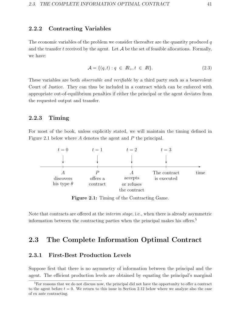
2.3. THE COMPLETE INFORMATION OPTIMAL CONTRACT 41
2.2.2 Contracting Variables
The economic variables of the problem we consider thereafter are the quantity produced q
and the transfer t received by the agent. Let A be the set of feasible allocations. Formally,
we have:
A = {(q, t) : q ∈ IR+, t ∈ IR}. (2.3)
These variables are both observable and verifiable by a third party such as a benevolent
Court of Justice. They can thus be included in a contract which can be enforced with
appropriate out-of-equilibrium penalties if either the principal or the agent deviates from
the requested output and transfer.
2.2.3 Timing
For most of the book, unless explicitly stated, we will maintain the timing defined in
Figure 2.1 below where A denotes the agent and P the principal.
-
time
? ? ??
t = 0 t = 1 t = 2 t = 3
Adiscovershis type θ
Poffers acontract
Aaccepts
or refusesthe contract
The contractis executed
Figure 2.1: Timing of the Contracting Game.
Note that contracts are offered at the interim stage, i.e., when there is already asymmetric
information between the contracting parties when the principal makes his offers.5
2.3 The Complete Information Optimal Contract
2.3.1 First-Best Production Levels
Suppose first that there is no asymmetry of information between the principal and the
agent. The efficient production levels are obtained by equating the principal’s marginal
5For reasons that we do not discuss now, the principal did not have the opportunity to offer a contractto the agent before t = 0. We return to this issue in Section 2.12 below where we analyze also the caseof ex ante contracting.

42 CHAPTER 2. THE RENT EXTRACTION-EFFICIENCY TRADE-OFF
value and the agent’s marginal cost. Hence, first-best outputs are given by the following
first-order conditions:
S ′(q∗) = θ (2.4)
and
S ′(q∗) = θ. (2.5)
The complete information efficient production levels q∗ and q∗ should be both carried out
if their social values, respectively W ∗ = S(q∗)− θq∗ − F and W ∗ = S(q∗)− θq∗ − F , are
non-negative. The social value of production when the agent is efficient, W ∗, is greater
than when he is inefficient, namely W ∗. Indeed, we have S(q∗) − θq∗ ≥ S(q∗) − θq∗ by
definition of q∗ and S(q∗)− θq∗ ≥ S(q∗)− θq∗ since θ > θ. For trade to be always carried
out, it is enough that production be socially valuable for the least efficient type, i.e., the
following condition must be satisfied:
W ∗ = S(q∗)− θq∗ − F ≥ 0, (2.6)
an hypothesis that we will maintain throughout this chapter. As the fixed cost F plays
no other role than justifying the existence of a single agent, it is set to zero from now on
in order to simplify notations.6
Note that, since the principal’s marginal value of output is decreasing, the optimal
production levels defined by (2.4) and (2.5) are such that q∗ > q∗, i.e., the optimal
production of an efficient agent is greater than that of an inefficient agent.
2.3.2 Implementation of the First-Best
For a successful delegation of the task, the principal must offer to the agent a utility
level which is at least as high as the utility level that the latter obtains outside the
relationship (for each value of the cost parameter). We refer to these constraints as the
agent’s participation constraints. If we normalize to zero the agent’s outside opportunity
utility level7 (sometimes called his status quo utility level), these participation constraints
write as:
t− θq ≥ 0 (2.7)
t− θq ≥ 0. (2.8)
To implement the first-best production levels, the principal can make the following
take-it-or-leave-it-offers to the agent: If θ = θ (resp. θ), the principal offers the transfer6We come back to the role of the fixed cost in Section 2.7.3 below.7This debatable assumption is relaxed in Section 3.4.

2.3. THE COMPLETE INFORMATION OPTIMAL CONTRACT 43
t∗ (resp. t∗) for the production level q∗ (resp. q∗) with t∗ = θq∗ (resp. t∗ = θq∗). Whatever
his type, the agent accepts the offer and makes then zero profit. The complete information
optimal contracts are thus (t∗, q∗) if θ = θ and (t∗, q∗) if θ = θ.
Importantly, under complete information, delegation is costless for the principal who
achieves the same utility level as what he would get if he was carrying the task himself
(of course with the same cost function as the agent).
2.3.3 A Graphical Representation of the Complete InformationOptimal Contract
In Figure 2.2, we draw the indifference curves of a θ-agent (solid curves) and of a θ-agent
(dotted curves) in the (q, t) space.
6
-
t
q!!!!!!!!!!!!!!!!!!!!!!!!
!!!!!!!!!!!!!!!!!!!!!!
!!!!!!!!!!!!!!!!!!!@
@I
t− θq = UÀ
t− θq = U
À
Figure 2.2: Indifference Curves of Both Types.
The iso-utility curves of both types of agent correspond to increasing levels of utility when
one moves in the north-west direction. Since θ > θ, the iso-utility curves of the inefficient
agent θ have a greater slope than those of the efficient agent. Thus, the iso-utility curves
for different types cross only once. All along this chapter and the next one, we will come
back several times to this important property called the single-crossing or Spence-Mirrlees
property.
The complete information optimal contract is finally represented in Figure 2.3 by the
pair of points (A∗, B∗). For each those two points, the strictly concave indifference curve

44 CHAPTER 2. THE RENT EXTRACTION-EFFICIENCY TRADE-OFF
of the principal is tangent to the zero rent iso-utility curve of the corresponding type.
Note that the iso-utility curves of the principal correspond to increasing levels of utility
when one moves in the south-east direction. The principal reaches thus a higher profit
when dealing with the efficient type. We denote by V ∗ (resp. V ∗) the principal’s level of
utility when he faces the θ− (resp. θ−) type. The principal having all bargaining power,
we have V ∗ = W ∗ (resp. V ∗ = W ∗).
6
-
t
q!!!!!!!!!!!!!!!!!!!!!!!!
@@I
•t∗
q∗
•t∗
q∗
B∗
A∗
SSSw
!!!!!!!!!!!
U∗ = t− θq = 0SSw ¡
¡¡ª
V ∗ = S(q)− t
?
U∗ = t− θq = 0
@@I
V ∗ = S(q)− t
Figure 2.3: First-Best Contracts.
Remark: In Figure 2.3, the payment t∗ is greater than t∗, but we note that t∗ can be
greater or smaller than t∗ depending on the curvature of the function S(·) as it can be
easily seen graphically.
2.4 Incentive Feasible Menu of Contracts
2.4.1 Incentive Compatibility and Participation
Suppose now that the marginal cost θ is the agent’s private information and let us consider
the case where the principal offers the menu of contracts {(t∗, q∗); (t∗, q∗)} hoping that an
agent with type θ will select (t∗, q∗) and an agent with type θ will select instead (t∗, q∗).
From Figure 2.3, we see that B∗ is preferred to A∗ by both types of agents. Indeed, the
θ-agent’s iso-utility curve which passes through B∗ corresponds to a positive utility level,
instead of a zero utility level at A∗. The θ-agent’s iso-utility curve which passes through
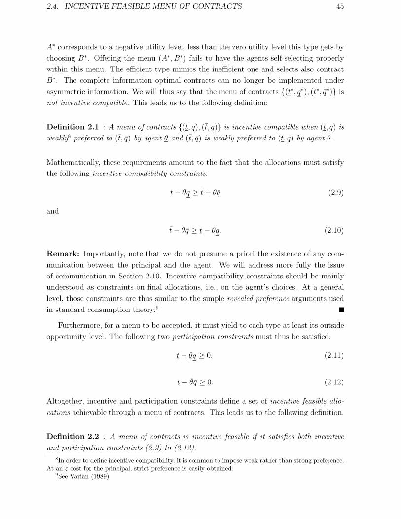
2.4. INCENTIVE FEASIBLE MENU OF CONTRACTS 45
A∗ corresponds to a negative utility level, less than the zero utility level this type gets by
choosing B∗. Offering the menu (A∗, B∗) fails to have the agents self-selecting properly
within this menu. The efficient type mimics the inefficient one and selects also contract
B∗. The complete information optimal contracts can no longer be implemented under
asymmetric information. We will thus say that the menu of contracts {(t∗, q∗); (t∗, q∗)} is
not incentive compatible. This leads us to the following definition:
Definition 2.1 : A menu of contracts {(t, q), (t, q)} is incentive compatible when (t, q) is
weakly8 preferred to (t, q) by agent θ and (t, q) is weakly preferred to (t, q) by agent θ.
Mathematically, these requirements amount to the fact that the allocations must satisfy
the following incentive compatibility constraints:
t− θq ≥ t− θq (2.9)
and
t− θq ≥ t− θq. (2.10)
Remark: Importantly, note that we do not presume a priori the existence of any com-
munication between the principal and the agent. We will address more fully the issue
of communication in Section 2.10. Incentive compatibility constraints should be mainly
understood as constraints on final allocations, i.e., on the agent’s choices. At a general
level, those constraints are thus similar to the simple revealed preference arguments used
in standard consumption theory.9
Furthermore, for a menu to be accepted, it must yield to each type at least its outside
opportunity level. The following two participation constraints must thus be satisfied:
t− θq ≥ 0, (2.11)
t− θq ≥ 0. (2.12)
Altogether, incentive and participation constraints define a set of incentive feasible allo-
cations achievable through a menu of contracts. This leads us to the following definition.
Definition 2.2 : A menu of contracts is incentive feasible if it satisfies both incentive
and participation constraints (2.9) to (2.12).
8In order to define incentive compatibility, it is common to impose weak rather than strong preference.At an ε cost for the principal, strict preference is easily obtained.
9See Varian (1989).

46 CHAPTER 2. THE RENT EXTRACTION-EFFICIENCY TRADE-OFF
The inequalities (2.9) to (2.12) fully characterize the set of incentive feasible menus of
contracts. The restrictions embodied in this set express, in addition to the usual condition
of voluntary trade, the constraints imposed on the allocation of resources by asymmetric
information between the principal and the agent.
2.4.2 Special Cases
• Bunching or Pooling Contracts: A first special case of incentive feasible menu
of contracts is obtained when the contracts targeted for each type coincide, i.e., when
t = t = tp, q = q = qp and both types of agents accept this contract. For those contracts,
we say that there is bunching or pooling of types.
The incentive constraints are all trivially satisfied by these contracts. Incentive com-
patibility is thus easy to satisfy, but at the cost of an obvious loss of flexibility in al-
locations which are no longer dependent on the state of nature. Only the participation
constraints matter now. However, the hardest participation constraint to satisfy is that
of the inefficient agent since (2.12) implies then (2.11) for a pooling contract.
• Shut-Down of the Least Efficient Type: Another particular case occurs when
one of the contracts is the null contract (0, 0) and the non-zero contract (ts, qs) is only
accepted by the efficient type. Then, (2.9) and (2.11) reduce both to:
ts − θqs ≥ 0. (2.13)
The incentive constraint of the bad type reduces also to:
0 ≥ ts − θqs. (2.14)
With such a contract, the principal gives up production if the agent is a θ-type. We will
say that it is a contract with shut-down.
As with the pooling contract just seen above, the benefit of the (0, 0) option is that it
somewhat reduces the number of constraints since the incentive (2.9) and the participation
(2.11) constraint take indeed the same form. Of course, the cost of such a contract may
be an excessive screening of types. Here, the screening of types takes the rather extreme
form of excluding the least efficient type.
2.4.3 Monotonicity Constraints
Incentive compatibility constraints reduce the set of feasible allocations. Moreover, in
well-behaved incentive problems, these constraints put lots of structure on the set of
feasible profiles of quantities. These quantities must generally satisfy a monotonicity

2.5. INFORMATION RENTS 47
constraint which does not exist under complete information. Indeed, in our simple model
adding (2.9) and (2.10) yields immediately:
q ≥ q. (2.15)
Independently of the principal’s preferences, incentive compatibility alone implies that the
production level requested from a θ-agent cannot be higher than the one requested from a
θ-agent. We will call condition (2.15) obtained by adding the two incentive constraints an
implementability condition. Any pair of outputs (q, q) which is implementable, i.e., which
can be reached by an incentive compatible contract, must satisfy this condition which is
here necessary and sufficient for implementability.
Remark: In our two-type model, the conditions for implementability take a simple form.
More generally, with more than two types or with a continuum, things might get harder
as we demonstrate in Appendix 2.1 and in Section 3.2.
2.5 Information Rents
To understand the structure of the optimal contract it is useful to introduce the concept
of information rent.
We saw in Section 2.2 that, under complete information, the principal (who has all
the bargaining power by assumption) is able to maintain all types of agents at their zero
status quo utility level. Their respective utility levels U∗ and U∗ at the first-best satisfy:
U∗ = t∗ − θq∗ = 0 (2.16)
and
U∗ = t∗ − θq∗ = 0. (2.17)
This will not be possible anymore in general under incomplete information, at least when
the principal wants both types of agents to be active.
Indeed, take any menu {(t, q); (t, q)} of incentive feasible contracts and consider the
utility level that a θ-agent would get by mimicking a θ-agent. By doing so, he would get
t− θq = t− θq + ∆θq = U + ∆θq. (2.18)
Even if the θ-agent utility level is reduced to its lowest utility level fixed at zero, i.e.,
U = t− θq = 0, the θ-agent benefits from an information rent which is worth ∆θq coming
from his ability to possibly mimic the less efficient type. So, as long as the principal

48 CHAPTER 2. THE RENT EXTRACTION-EFFICIENCY TRADE-OFF
insists on a positive output, q > 0, the principal must give up a positive rent to a θ-agent.
This information rent is generated by the informational advantage of the agent over the
principal. The principal’s problem is to determine the smartest way to give up such a
rent provided by any given incentive feasible contract.
In what follows, we use the notations U = t − θq and U = t − θq to denote the
respective information rent of each type.
2.6 The Optimization Program of the Principal
According to our timing of the contractual game, the principal must offer a menu of
contracts before knowing which type of agent he is facing. Therefore, he will compute the
benefit of any menu of contracts {(t, q); (t, q)} in expected terms. The principal’s problem
writes thus as:
(P ) : max{(t,q);(t,q)}
ν(S(q)− t
)+ (1− ν) (S(q)− t)
subject to (2.9) to (2.12).
Using the definition of the information rents U = t− θq and U = t− θq, we can replace
transfers in the principal’s objective function as functions of information rents and outputs
so that the new optimization variables are now {(U, q); (U , q)}. This change of variables
will sharpen our economic interpretations all along the book. The focus on information
rents allows us to assess the distributive impact of asymmetric information. The focus on
outputs allows us to analyze also its impact on allocative efficiency and the overall gains
from trade.
With this change of variables, the principal’s objective function can then be rewritten
as:
ν(S(q)− θq
)+ (1− ν)
(S(q)− θq
)︸ ︷︷ ︸Expected Allocative Efficiency
− (νU + (1− ν)U
).︸ ︷︷ ︸
Expected Information Rent
(2.19)
This new expression shows clearly that the principal wishes to maximize the expected
social value of trade minus the expected rent of the agent.10 The principal is ready to
accept some distortions away from efficiency to decrease the agent’s information rent. We
see below precisely how.
10Note that a social utility maximizer putting an equal weight on the principal and the agent’s expectedutility in his objective function would be interested in maximizing expected allocative efficiency only,without any concern for the distribution of information rents between the principal and the agent.

2.7. THE RENT EXTRACTION-EFFICIENCY TRADE-OFF 49
The incentive constraints (2.9) and (2.10) written in terms of information rents and
outputs are respectively:
U ≥ U + ∆θq, (2.20)
U ≥ U −∆θq. (2.21)
The participation constraints (2.11) and (2.12) become respectively:
U ≥ 0, (2.22)
U ≥ 0. (2.23)
The principal wishes to solve problem (P ) below:
(P ) : max{(U,q);(U ,q)}
ν(S(q)− θq) + (1− ν)(S(q)− θq)− (νU + (1− ν)U)
subject to (2.20) to (2.23).
We index with a superscript SB meaning “second-best” the solution to this problem.
2.7 The Rent Extraction-Efficiency Trade-Off
2.7.1 The Asymmetric Information Optimal Contract
The major difficulty of problem (P ), and more generally of incentive theory, is to deter-
mine which of the many constraints imposed by incentive compatibility and participation
are the relevant ones, i.e., the binding ones at the optimum of the principal’s problem.
A first route could be to apply Lagrangean techniques to problem (P ), once one has
checked that the problem is concave. The number of constraints calls nevertheless for a
more practical route where the modeler first guesses which are the binding constraints and
checks ex post that the omitted constraints are indeed strictly satisfied. In a well-behaved
incentive problem, this route is certainly more fruitful. In our very simple model, such
a strategy provides a quick solution to the optimization problem. Moreover, this route
turns out to be more fruitful to build the economic intuition behind this model.
Let us first consider contracts with q > 0. The ability of the θ-agent to mimic the θ-
agent implies that the θ-agent’s participation constraint (2.22) is always strictly satisfied.
Indeed, (2.23) and (2.20) imply immediately (2.22). If a menu of contracts enables an
inefficient agent to reach his status quo utility level, it will be also the case for an efficient

50 CHAPTER 2. THE RENT EXTRACTION-EFFICIENCY TRADE-OFF
agent who can produce at a lower cost. Second, (2.21) seems also irrelevant since, as
guessed from Section 2.4, the difficulty comes from a θ-agent willing to claim that he is
inefficient rather than the reverse.
This simplification in the number of relevant constraints leaves us with only two re-
maining constraints, the θ-agent’s incentive constraint (2.20) and the θ-agent’s participa-
tion constraint (2.23). Of course, both constraints must be binding at the optimum of
the principal’s problem (P ). Indeed, suppose it is not so; then the principal could either
reduce U or (and) U by a small amount ε, still keeping all outputs the same. This would
increase the principal’s payoff leading to a contradiction. Hence, we must have:
U = ∆θq, (2.24)
and
U = 0. (2.25)
Substituting (2.24) and (2.25) into (2.19), we obtain a reduced program (P ′) with outputs
as the only choice variables:
(P ′) : max{(q,q)}
ν(S(q)− θq
)+ (1− ν)
(S(q)− θq
)− ν∆θq.
Compared with the full information setting, asymmetric information alters the principal’s
optimization simply by the subtraction of the expected rent which has to be given up to
the efficient type. The inefficient type gets no rent, but the efficient type θ gets the
information rent that he could obtain anyway by mimicking the inefficient type θ. This
rent depends only on the level of production requested from this inefficient type.
Since the expected rent given up does not depend on the production level q of the
efficient type, the maximization of (P ′) calls for no distortion away from the first-best for
the efficient type’s output, namely:
S ′(qSB) = θ or qSB = q∗. (2.26)
However, maximization with respect to q yields now:
(1− ν)(S ′(qSB)− θ
)= ν∆θ. (2.27)
Increasing the inefficient agent’s output by an infinitesimal amount dq increases allocative
efficiency in this state of nature. The principal’s expected payoff is improved by a term
equal to the left-hand side of (2.27) times dq. At the same time, this infinitesimal change
in output also increases the efficient agent’s information rent and the principal’s expected
payoff is diminished by a term equal to the right-hand side above times dq.
At the second-best optimum, the principal is neither willing to increase nor to de-
crease the inefficient agent’s output and (2.27) expresses the important trade-off between

2.7. THE RENT EXTRACTION-EFFICIENCY TRADE-OFF 51
efficiency and rent extraction which arises under asymmetric information. The expected
marginal efficiency cost and the expected marginal cost of the rent brought about by an
infinitesimal change of the inefficient type’s output are equated.
For further references, it is useful to summarize the main features of the optimal
contract.
Proposition 2.1 : Under asymmetric information, the optimal menu of contracts en-
tails:
• No output distortion for the efficient type with respect to the first-best, qSB = q∗. A
downward output distortion for the inefficient type, qSB < q∗ with
S ′(qSB) = θ +ν
1− ν∆θ. (2.28)
• Only the efficient type gets a strictly positive information rent given by
USB = ∆θqSB. (2.29)
• The second-best transfers are given by tSB = θq∗ + ∆θqSB and tSB = θqSB.
To validate our approach based on the sole consideration of the efficient type’s incentive
constraint, it remains to check that the omitted incentive constraint of an inefficient agent
is satisfied, i.e., 0 ≥ ∆θqSB−∆θqSB. This latter inequality follows from the monotonicity
of the second-best schedule of outputs since we have indeed qSB = q∗ > q∗ > qSB.
2.7.2 A Graphical Representation of the Second-Best Outcome
Starting from the complete information optimal contract (A∗, B∗) which is not incentive
compatible, we can construct an incentive compatible contract (B∗, C) with the same
production levels by giving a higher transfer to the agent producing q∗. (See Figure 2.4).

52 CHAPTER 2. THE RENT EXTRACTION-EFFICIENCY TRADE-OFF
6
0
-
t
q!!!!!!!!!!!!!!!!!!!!!!!!!!
•
q∗
A∗
!!!!!!!!!!!!!!!!!!!!!!!!•C
@@@I
•B∗
q∗
t∗
t∗
V ∗ = S(q)− t
U = t− θq = ∆θq∗
U∗ = t− θq = 0
V ∗ = S(q)− t
?
¾
¢¢®
HHHY
?
U∗ = t− θq = 0
Figure 2.4: Necessary Rent to Implement the First-Best Outputs.
The contract C is on the θ-agent’s indifference curve passing through B∗. Henceforth, the
θ-agent is now indifferent between B∗ and C and (B∗, C) becomes an incentive compatible
menu of contracts. The rent which is given up to the θ-firm is now ∆θq∗.
Rather than insisting on the first-best production level for an inefficient type, the
principal prefers actually to slightly decrease q by an amount dq. By doing so, expected
efficiency is just diminished by a second-order term, since q∗ is the first-best output which
maximizes efficiency when the agent is inefficient. Instead, the information rent left to
the efficient type diminishes to the first-order. Of course, the principal stops reducing the
inefficient type’s output until a further decrease would have a greater efficiency cost than
the gain in reducing the information rent it would bring about. The optimal trade-off
finally occurs at (ASB, BSB) as shown on Figure 2.5.

2.7. THE RENT EXTRACTION-EFFICIENCY TRADE-OFF 53
6
0
-
t
q!!!!!!!!!!!!!!!!!!!!!!!!!!
•
q∗
A∗
!!!!!!!!!!!!!!!!!!!!!!!!•C
!!!!!!!!!!!!!!!!!!!!!!!!!•ASB
•B∗
q∗
t∗
t∗
•BSB
qSB
tSB
USB = t− θq = 0V SB = S(q)− t
V SB = S(q)− t
USB = t− θq = ∆θqSB
tSB!!!!!!!!!!!!!!!!!!!?
»»»»»9
»»9
¾
Figure 2.5: Optimal Second-Best Contracts ASB and BSB.
2.7.3 Shut-Down Policy
If the first-order condition (2.28) has no positive solution, qSB should be set at zero. We
are in the special case of a contract with shut-down. BSB coincides with 0 and ASB with
A∗ in Figure 2.5. Then, no rent is given up to the θ-firm by the unique non null contract
(t∗, q∗) offered and only selected by agent θ. The shut-down of the agent occurs when
θ = θ. With such a policy, a significant inefficiency emerges since the inefficient type does
not produce. The benefit of such a policy is that no rent is given up to the efficient type.
More generally, such a shut-down policy is optimal when
ν(S(q∗)− θq∗
) ≥ ν(S(qSB)− θqSB −∆θqSB
)+ (1− ν)
(S(qSB)− θqSB
)(2.30)
or, noting that q∗ = qSB, when
ν∆θqSB ≥ (1− ν)(S(qSB)− θqSB
). (2.31)
The left-hand side of (2.31) represents the expected cost of the efficient type’s rent due to
the presence of the inefficient one when the latter produces a positive amount qSB. The
right-hand side of (2.31) represents instead the expected benefit from transacting with
the inefficient type at the second-best level of output. Shut-down of the inefficient type
is optimal when this expected benefit is lower than the expected cost.

54 CHAPTER 2. THE RENT EXTRACTION-EFFICIENCY TRADE-OFF
Remark: Looking again at condition (2.28), we see that shut-down is never desirable
when the Inada condition S ′(0) = +∞ is satisfied. Indeed, qSB defined by (2.28) is
necessarily strictly positive. Then, note that we can rewrite S(qSB)− (θ + ν
1−ν∆θ
)qSB as
S(qSB)−S ′(qSB)qSB which is strictly positive since S(q)−S ′(q)q is strictly increasing with
q when S ′′(·) < 0 and is equal to zero for q = 0. Hence, S(qSB) − (θ + ν
1−ν)∆θ
)qSB > 0
and shut-down of the least efficient type does not occur.
The shut-down policy is also dependent of the status quo utility levels. Suppose that,
for both types, the status quo utility level is U0 > 0. Then (2.31) becomes (dividing by
1− ν)
ν
1− ν∆θqSB + U0 ≥ S(qSB)− θqSB. (2.32)
Therefore, for ν large enough, shut-down occurs11 even if the Inada condition S ′(0) =
+∞ is satisfied. Note that this case also occurs when the agent has a strictly positive
fixed cost F > 0.
Coming back to the principal’s problem (P ), the occurrence of shut-down can also be
interpreted as saying that the principal has, on top of the agent’s production, another
choice variable to solve the screening problem. This extra variable is the subset of types
which are induced to produce a positive amount. Reducing the subset of producing agents
obviously reduces the rent of the most efficient type. In our two-type model exclusion of
the least efficient type may thus be optimal.
2.8 The Theory of the Firm under Asymmetric In-
formation
When the delegation of task occurs within the firm, a major conclusion of the above
analysis is that, because of asymmetric information, the firm does not maximize the social
value of trade, or more precisely its profit, a maintained assumption of most economic
theory. This lack of allocative efficiency should not be considered as a failure in the
rational use of resources within the firm. Indeed, the point is that allocative efficiency
is only one part of the principal’s objective. The allocation of resources within the firm
remains constrained optimal once informational constraints are fully taken into account.
This systematic deviation away from profit maximization can be interpreted as an “X-
inefficiency” a la Leibenstein (1966). This author has indeed stressed the management
failures which take place within the largest firms, i.e., those which are the most likely to
suffer from significant internal informational problems.11Suppose the contrary. Then qSB goes to zero as ν goes to one and S(qSB)−θqSB as well as ν
1−ν ∆θqSB
go to zero. But then (2.32) must hold strictly for ν close enough to one.

2.9. ASYMMETRIC INFORMATION AND MARGINAL COST PRICING 55
Williamson (1975) has also pushed forward the view that various transaction costs may
impede the achievement of economic transactions. Among the many origins of these costs,
Williamson stresses “informational impactedness” as an important source of inefficiency.
Clearly, even in a world with a costless enforcement of contracts, a major source of
allocative inefficiency is the existence of asymmetric information between trading partners.
Of course, another important insight of Williamson’s analysis is that transaction costs
may be mitigated by the choice of convenient organizational forms. This point does not
contradict our interpretation of transaction costs as coming from informational problems
if one is ready to accept the view that various organizational forms generate different
degrees and costs of asymmetric information between partners, an issue which is clearly
high on the current research agenda of organization theory.12
The idea that various organizational forms are associated with different information
structures has been used by some authors to provide a theory of vertical integration.
Arrow (1975) suggests that an upstream firm may want to integrate backward and ac-
quire a downstream supplier to reduce the extent of asymmetric information between
those two units. An obvious limitation of this approach is that it takes as exogenous the
fact that vertical integration improves information. This exogeneity has led to an impor-
tant debate over the last fifteen years between proponents of this idea (like for instance
Williamson (1985)) and opponents (like Grossman and Hart (1986)) who would prefer to
see information structures being derived from the property rights associated with different
organizational forms.
A last point is worth stressing. Even though asymmetric information generates al-
locative inefficiencies, those inefficiencies do not call for any public policy motivated by
efficiency. Indeed, any benevolent policy maker in charge of correcting these inefficiencies
would face the same informational constraints as the principal. The allocation obtained
above is Pareto optimal in the set of incentive feasible allocations or incentive Pareto
optimal. Nevertheless, the policy-maker might want to implement different trade-offs be-
tween efficiency and rent extraction as we will see in Section 2.16.1 in the archetypical
case of regulatory intervention. Redistribution would be then the motivation for public
policy.
2.9 Asymmetric Information and Marginal Cost Pric-
ing
Let us view the principal as acting for a set of consumers and the agent as a firm producing
a consumption good. The first-best rules defined by (2.4) and (2.5) can be interpreted
12Aghion and Tirole (1997) for instance.

56 CHAPTER 2. THE RENT EXTRACTION-EFFICIENCY TRADE-OFF
as price equal to marginal cost since consumers on the market will equate their marginal
utility of consumption to price.
Under asymmetric information, price equates marginal cost only when the producing
firm is efficient (θ = θ). Using (2.28), we immediately get the expression of the price p(θ)
for the inefficient type’s output:
p(θ) = θ +ν
1− ν∆θ. (2.33)
Price is higher than marginal cost to decrease the quantity q produced by the inefficient
firm, and reduce the efficient firm’s information rent. Alternatively, we can say that price
is equal to a generalized (or virtual13) marginal cost which includes, in addition to the
traditional marginal cost of the inefficient type θ, an information cost which is worth
here ν1−ν
∆θ. What is simply required is to generalize the concept of cost to include the
information cost imposed by asymmetric information.
2.10 The Revelation Principle
In the above analysis, we have restricted the principal to offer a menu of contracts, one for
each possible type. First, one may wonder if a better outcome could be achieved with a
more complex contract allowing the agent to possibly choose among more options. Second,
one may also wonder whether some sort of communication device between the agent and
the principal could be used to transmit information to the principal so that the latter
can recommend outputs and payments as a function of transmitted information. This is
not the case. Indeed, the Revelation Principle ensures that there is no loss of generality
in restricting the principal to offer simple menus having at most as many options as
the cardinality of the type space. Those simple menus are actually examples of direct
revelation mechanisms for whom we give now a couple of definitions.
Definition 2.3 : A direct revelation mechanism is a mapping g(·) from Θ to A which
writes as g(θ) = (q(θ), t(θ)) for all θ belonging to Θ. The principal commits to offer the
transfer t(θ) and the production level q(θ) if the agent announces the value θ for all θ in
Θ.
Definition 2.4 : A direct revelation mechanism g(·) is truthful if it is incentive com-
patible for the agent to announce his true type, for any type, i.e., if the direct revelation
mechanism satisfies the following incentive compatibility constraints:
t(θ)− θq(θ) ≥ t(θ)− θq(θ) (2.34)
t(θ)− θq(θ) ≥ t(θ)− θq(θ). (2.35)13To use the expression coined by Myerson (1979).

2.10. THE REVELATION PRINCIPLE 57
Denoting transfer and output for each possible report respectively as t(θ) = t, q(θ) = q,
t(θ) = t and q(θ) = q, we get back to the notations of the previous sections and in
particular to the incentive constraints (2.9) and (2.10).
A more general mechanism can be obtained when communication between the principal
and the agent is more complex than having simply the agent report his type to the
principal. Let M be the message space offered to the agent by a more general mechanism.
This message space can be as complex as one can imagine. Conditionally on a given
message m received from the agent, the principal requests a production level q(m) and
provides a corresponding payment t(m).
Definition 2.5 : A mechanism is a message space M and a mapping g(·) from M to Awhich writes as g(m) = (q(m), t(m)) for all m belonging to M.
When facing such a mechanism, the agent with type θ chooses a best message m∗(θ)which14 is implicitly defined as
t(m∗(θ))− θq(m∗(θ)) ≥ t(m)− θq(m) for all m in M. (2.36)
The mechanism (M, g(·)) induces therefore an allocation rule a(θ) = (q(m∗(θ)), t(m∗(θ))mapping the set of types Θ into the set of allocations A. Then, we are ready to state the
Revelation Principle in the one agent case.
Proposition 2.2 : Any allocation rule a(θ) obtained with a mechanism (M, g(·)) can
also be implemented with a direct and truthful revelation mechanism.
Proof: The indirect mechanism (M, g(·)) induces an allocation rule a(θ) = (q(m∗(θ)), t(m∗(θ))from Θ into A. By composition of g(·) and m∗(·), we can construct a direct revela-
tion mechanism g(·) mapping Θ into A, namely g = g ◦ m∗, or more precisely g(θ) =
(q(θ), t(θ)) ≡ g(m∗(θ)) = (q(m∗(θ)), t(m∗(θ))) for all θ in Θ.
Figure 2.6 illustrates this construction which is at the core of the Revelation Principle:
- -Θ M Am∗(·) g(·)
6
g(·) = g ◦m∗(·)
14Possibly, the agent’s best response can be a correspondence without changing anything below; justpick one of the possible maximizers and call it m∗(θ).

58 CHAPTER 2. THE RENT EXTRACTION-EFFICIENCY TRADE-OFF
Figure 2.6: The Revelation Principle.
We check now that the direct revelation mechanism g(·) is truthful. Indeed, since
(2.36) is true for all m, it holds in particular for m = m∗(θ′) for any θ′ in Θ. We have
thus:
t(m∗(θ))− θq(m∗(θ)) ≥ t(m∗(θ′))− θq(m∗(θ′)) for all (θ, θ′) in Θ2. (2.37)
Finally, using the definition of g(·), we get:
t(θ)− θq(θ) ≥ t(θ′)− θq(θ′) for all (θ, θ′) in Θ2. (2.38)
Hence, the direct revelation mechanism g(·) is truthful.
Importantly, the Revelation Principle provides a considerable simplification of contract
theory since it enables us to restrict the analysis to a simple and well defined family of
functions, the truthful direct revelation mechanisms.
Gibbard (1973) characterized the dominant strategy (non random) mechanisms
(mappings from arbitrary strategy spaces into allocations) when feasible allocations be-
long to a finite set and when there is no a priori information on the players’ preferences
(which are strict orderings). Actually he showed that such mechanisms had to be dicta-
torial, i.e., they had to correspond to the optimal choice of single agent. As a corollary he
showed that any voting mechanism (i.e., direct revelation mechanism) for which the truth
was a dominant strategy was also dictatorial. In this environment anything achievable by
a dominant strategy mechanism can be achieved by a truthful direct revelation mecha-
nism. So, Gibbard proved one version of the Revelation Principle indirectly. For the case
of quasi-linear preferences, Green and Laffont (1977) defined dominant strategy truthful
direct revelation mechanisms and proved directly that for any other dominant strategy
mechanism there is an equivalent truthful direct revelation mechanism (and they char-
acterized the class of truthful direct revelation mechanisms). Dasgupta, Hammond and
Maskin (1979) extended this direct proof to any family of preferences. Myerson (1979)
extended this proof to Bayesian implementation. Those notions of implementation must
be analyzed in multi-agent environments which are out of the scope of the present book.
They will be studied in Volume II. The expression “The Revelation Principle” finally
appeared in Baron and Myerson (1982).
2.11 A More General Utility Function for the Agent
Still keeping quasi-linear utility functions, let U = t−C(q, θ) be now the agent’s objective
function with Cq(·) > 0, Cθ(·) > 0, Cqq(·) > 0 and Cqqθ(·) > 0. The generalization of
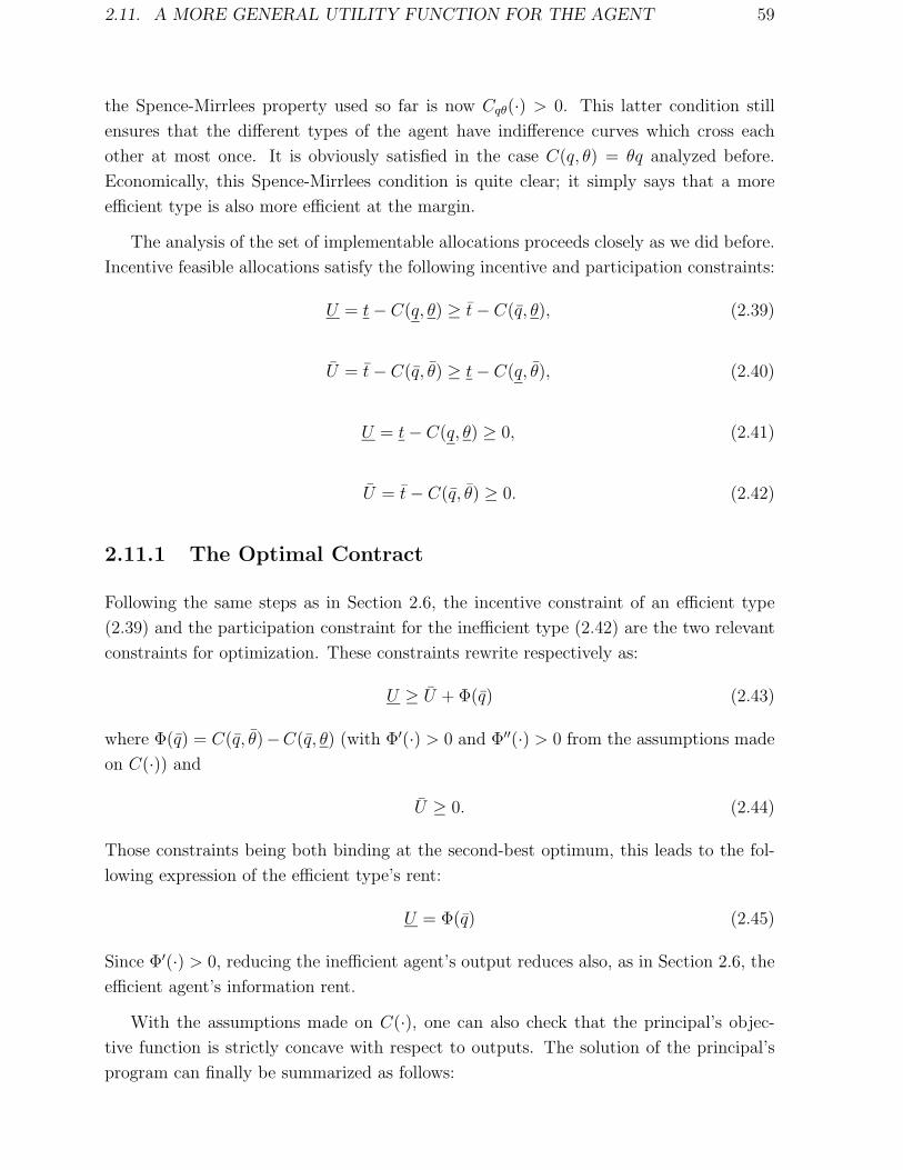
2.11. A MORE GENERAL UTILITY FUNCTION FOR THE AGENT 59
the Spence-Mirrlees property used so far is now Cqθ(·) > 0. This latter condition still
ensures that the different types of the agent have indifference curves which cross each
other at most once. It is obviously satisfied in the case C(q, θ) = θq analyzed before.
Economically, this Spence-Mirrlees condition is quite clear; it simply says that a more
efficient type is also more efficient at the margin.
The analysis of the set of implementable allocations proceeds closely as we did before.
Incentive feasible allocations satisfy the following incentive and participation constraints:
U = t− C(q, θ) ≥ t− C(q, θ), (2.39)
U = t− C(q, θ) ≥ t− C(q, θ), (2.40)
U = t− C(q, θ) ≥ 0, (2.41)
U = t− C(q, θ) ≥ 0. (2.42)
2.11.1 The Optimal Contract
Following the same steps as in Section 2.6, the incentive constraint of an efficient type
(2.39) and the participation constraint for the inefficient type (2.42) are the two relevant
constraints for optimization. These constraints rewrite respectively as:
U ≥ U + Φ(q) (2.43)
where Φ(q) = C(q, θ)−C(q, θ) (with Φ′(·) > 0 and Φ′′(·) > 0 from the assumptions made
on C(·)) and
U ≥ 0. (2.44)
Those constraints being both binding at the second-best optimum, this leads to the fol-
lowing expression of the efficient type’s rent:
U = Φ(q) (2.45)
Since Φ′(·) > 0, reducing the inefficient agent’s output reduces also, as in Section 2.6, the
efficient agent’s information rent.
With the assumptions made on C(·), one can also check that the principal’s objec-
tive function is strictly concave with respect to outputs. The solution of the principal’s
program can finally be summarized as follows:

60 CHAPTER 2. THE RENT EXTRACTION-EFFICIENCY TRADE-OFF
Proposition 2.3 : With general preferences satisfying the Spence-Mirrlees property, Cθq >
0, the optimal menu of contracts entails:
• No output distortion with respect to the first-best outcome for the efficient type,
qSB = q∗ with
S ′(q∗) = Cq(q∗, θ). (2.46)
A downward output distortion for the inefficient type, qSB < q∗ with
S ′(q∗) = Cq(q∗, θ) (2.47)
and
S ′(qSB) = Cq(qSB, θ) +
ν
1− νΦ′(qSB). (2.48)
• Only the efficient type gets a strictly positive information rent given by USB =
Φ(qSB).
• The second-best transfers are respectively given by tSB = C(q∗, θ) + Φ(qSB) and
tSB = C(qSB, θ).
The first-order conditions (2.46), (2.48) characterize the optimal solution if the ne-
glected incentive constraint (2.40) is satisfied. For this to be true, we need to have:
tSB − C(qSB, θ) ≥ tSB − C(qSB, θ) + C(qSB, θ)− C(qSB, θ), (2.49)
which amounts to
0 ≥ Φ(qSB)− Φ(qSB). (2.50)
We have Φ′(·) > 0 from the Spence-Mirrlees condition, hence (2.50) yields qSB ≤ qSB.
But, from our assumptions: qSB = q∗ > q∗ > qSB.15 So the Spence-Mirrlees condition
guarantees that only the efficient type’s incentive constraint has to be taken into account.
The critical role of the Spence-Mirrlees condition to simplify the problem will appear
even more clearly in models with more than two types.16
15Indeed, by definition of q∗, S′(q∗) = Cq(q∗, θ) < Cq(q∗, θ) since Cqθ > 0. Hence, using the fact thatS(q) − C(q, θ) is concave in q and maximum for q∗, we have q∗ > q∗. Moreover, Φ′(·) > 0 implies thatS′(qSB) > Cq(qSB , θ). Hence, we have also qSB < q∗.
16See Section 3.2 and Appendix 2.1 below.

2.11. A MORE GENERAL UTILITY FUNCTION FOR THE AGENT 61
Remark: The Spence-Mirrlees property is more generally a constant sign condition17 on
Cθq. If Cθq < 0, Proposition 2.3 is unchanged except that now the inefficient type’s output
is distorted upwards qSB > q∗ > q∗. Indeed, in such a model, the first-best production
level of the inefficient type is higher than for the efficient type. Moreover, the information
rent of the efficient type is still Φ(q) = C(q, θ) − C(q, θ), but now to decrease this rent
requires an increase of q since Cθq < 0.
2.11.2 Non-Responsiveness
Let us come back to our linear specification of the agent’s cost function, but let us also
assume that the principal’s return from contracting depends directly on θ and writes as
S(q, θ). This is an instance of a common value model where the agent’s type directly
affects the principal’s utility function. On top of the usual assumptions of a positive
and decreasing marginal value of trade, we also assume that Sqθ(q, θ) > 1. This latter
assumption simply means that the marginal gross value of trade for the principal increases
sharply with the agent’s type. For instance, the efficient agent produces a lower quality
good than the inefficient one and the principal prefers a high quality good.
The first-best productions are now defined by Sq(q∗, θ) = θ and Sq(q
∗, θ) = θ. With
our assumption on Sqθ, the first-best production schedule is such that q∗ < q∗, i.e., it does
not satisfy the monotonicity condition (2.15) implied by incentive compatibility.
In this case, there exists a strong conflict between the principal’s desire to have the
θ-type produce more than the θ-agent for pure efficiency reasons and the monotonicity
condition due to asymmetric information. This is what Guesnerie and Laffont (1984) call a
phenomenon of non-responsiveness in their general analysis of the principal-agent’s model
with a continuum of types. This phenomenon makes screening of types quite difficult.
Indeed, the second-best optimum induces screening only when qSB = q∗ and qSB defined
by:
Sq(qSB, θ) = θ +
ν
1− ν∆θ (2.51)
satisfy the monotonicity condition qSB ≥ qSB. However, when ν is small enough, qSB
defined on (2.51) is close to the first-best outcome q∗ and thus qSB > qSB which violates
the monotonicity condition (2.15). Hence, non-responsiveness forces the principal to use
a pooling allocation. Figure 2.7 illustrates this non-responsiveness.
17In Guesnerie and Laffont (1984), the Spence-Mirrlees condition is called the constant sign (CS+ orCS−) assumption.

62 CHAPTER 2. THE RENT EXTRACTION-EFFICIENCY TRADE-OFF
-
6
t
q""
""
""
""
""
""
""
""
""
""
""
"""
t = θq
··························
t = θq
•B∗
q∗
•D
q∗
•E
•A∗
•C
qp
W = S(q, θ)− t
W = νS(q, θ) + (1− ν)S(q, θ)− t
W = S(q, θ)− t
t∗
t∗
JJ
@@I
©©¼
HHY
@@@I
Figure 2.7: Non-Responsiveness.
As in Figure 2.4, the pair of first-best contracts (A∗, B∗) is not incentive compatible.
But, contrary to the case of Section 2.7.2, the contract C which makes the θ-type being
indifferent between telling the truth and taking contract A∗ is not incentive compatible
for the θ-type who also strictly prefers C to A∗.
One possibility to restore incentive compatibility would be to distort q∗ down to q∗
to decrease the θ-type’s information rent to contract D while still preserving incentive
compatibility for both types. We would obtain then a pooling allocation at D. The
principal can do better by choosing another pooling allocation which is obtained by moving
along the zero iso-utility line of a θ-type. Indeed, the best pooling allocation solves
problem (P ) below:
(P ) : max{(qp,tp)}
νS(qp, θ) + (1− ν)S(qp, θ)− tp
subject to
tp − θqp ≥ 0 (2.52)
tp − θqp ≥ 0. (2.53)
The harder participation constraint is obviously that of the least efficient type, namely

2.11. A MORE GENERAL UTILITY FUNCTION FOR THE AGENT 63
(2.53). Hence, the optimal solution is characterized by
νSq(qp, θ) + (1− ν)Sq(q
p, θ) = θ, (2.54)
and
tp = θqp (2.55)
with qp < q∗ since Sqθ > 0.
This pooling contract is represented by point E in Figure 2.6 (which can be to the left
or to the right of D) where the heavy line indifference curve of the principal corresponds
to the “average” utility function S(q)− t = νS(q, θ) + (1− ν)S(q, θ)− t.
Importantly, when non-responsiveness occurs, the sharp conflict between the prin-
cipal’s preferences and the incentive constraints (which reflect the agent’s preferences)
makes impossible the use of any information transmitted by the agent about his type.
2.11.3 More Than Two Goods
Let us now assume that the agent is producing a whole vector of goods q = (q1, . . . , qn) for
the principal. The agent’s cost function becomes C(q, θ) with C(·) being strictly convex
in q. The value for the principal of consuming this whole bundle is now S(q) with also
S(·) being strictly concave in q.
In this “multi-output” incentive problem, the principal is interested by a whole set of
activities carried out simultaneously by the agent. It is straightforward to check that the
efficient agent’s information rent writes now as U = Φ(q) with Φ(q) = C(q, θ)− C(q, θ).
This leads to the following second-best optimal outputs. The efficient type produces
the first-best vector of outputs qSB = q∗ with
Sqi(q∗) = Cqi
(q∗, θ) for all i in {1, . . . , n}. (2.56)
The inefficient type’s vector of outputs qSB is instead characterized by:
Sqi(qSB) = Cqi
(qSB, θ) +ν
1− νΦqi
(qSB), for all i in {1, . . . , n}, (2.57)
which generalizes the distortion of unidimensional models.
Without specifying further the value and cost functions, it is a priori hard to compare
these second-best outputs above with the first-best outputs defined by the n first-order
conditions:
Sqi(q∗) = Cqi
(q∗, θ). (2.58)

64 CHAPTER 2. THE RENT EXTRACTION-EFFICIENCY TRADE-OFF
Indeed, it may well be the case that the n first-order conditions (2.57) define altogether
a vector of outputs with some components qSBi above q∗i for a subset of indices i.
Turning now to incentive compatibility, and summing the incentive constraints U ≥U + Φ(q) and U ≥ U − Φ(q) for any incentive feasible contract yields:
C(q, θ)− C(q, θ) ≥ C(q, θ)− C(q, θ) (2.59)
for all implementable pairs (q, q).
Obviously, this condition is satisfied if the Spence-Mirrlees conditions Cqiθ(·) > 0 holds
for each output i and if the monotonicity conditions qi < qifor all i are all satisfied. In
this case, the neglected incentive constraint of a θ-agent is automatically satisfied when
qSBi < q∗i = qSB
ifor all i. However, the reverse is not true; it might well be the case that
qSBi > qSB
i= q∗
ifor some output i and the condition (2.59) nevertheless holds for the
second-best vector of outputs q∗ and qSB.
2.12 Ex Ante Versus Ex Post Participation Constraints
As we have already mentioned, for most of the book dealing with the case of adverse
selection, we consider the case of contracts offered at the interim stage. Sometimes, the
principal and the agent can nevertheless contract also at the ex ante stage, i.e., before
the agent discovers his type. For instance, the contours of the firm may be designed
before the agent receives any piece of information on his productivity. In this section, we
characterize for this alternative timing the optimal contract under various assumptions
about the risk aversion of the two players.
2.12.1 Risk Neutrality
Suppose that, instead of contracting after the agent has discovered θ, the principal and
the agent meet and contract ex ante, i.e., before the agent’s learning of information. If
the agent is risk neutral, his ex ante participation constraint writes now as:
νU + (1− ν)U ≥ 0. (2.60)
This ex ante participation constraint replaces the two ex post participation constraints
(2.22) and (2.23) in problem (P ). What matters now to insure participation is that the
agent’s expected information rent remains non-negative.
From (2.19), we see that the principal’s objective function is decreasing in the agent’s
expected information rent. Ideally, the principal wants to impose a zero expected rent to
the agent and have (2.60) being binding.

2.12. EX ANTE VERSUS EX POST PARTICIPATION CONSTRAINTS 65
Moreover, the principal must structure the ex post rents U and U to ensure that the
wedge between those two levels is such that the incentive constraints (2.20) and (2.21)
remain satisfied. An example of such a rent allocation which is both incentive compatible
and satisfies the ex ante participation constraint with an equality is:
U∗ = (1− ν)∆θq∗ > 0 and U∗ = −ν∆θq∗ < 0. (2.61)
With such a rent distribution, the optimal contract implements the first-best outputs
costlessly from the principal’s point of view. Note however that the first-best may not be
monotonic as requested by the implementability condition. This is for instance the case
when the non-responsiveness property holds as in Section 2.11.2. In that case, even under
ex ante contracting and risk neutrality, some inefficiency still arises.18
In the contract defined by (2.61), the agent is rewarded when he is efficient and
punished when he turns out to be inefficient. There must be some risk on the distribution
of information rents to induce information revelation, but this risk is costless for the
principal because of the agent’s risk neutrality. However, to be feasible, such an ex ante
contract requires a strong ability of the Court of Justice to enforce contracts leading
possibly to a negative payoff when a bad state of nature realizes.19
Remark: The principal has much more leeway in structuring the rents U and U so that
the incentive constraints (2.20) and (2.21) hold and the ex ante participation constraint
(2.60) is an equality. Consider the following contracts {(t∗, q∗); (t∗, q∗)} where t∗ = S(q∗)−T and t∗ = S(q∗)−T with T being a lump-sum payment to be defined below. This contract
is incentive compatible since:
t∗ − θq∗ = S(q∗)− θq∗ − T > t∗ − θq∗ = S(q∗)− θq∗ − T (2.62)
by definition of q∗ and
t∗ − θq∗ = S(q∗)− θq∗ − T > t∗ − θq∗ = S(q∗)− θq∗ − T, (2.63)
by definition of q∗.
Note that the incentive compatibility constraints are now strict inequalities. Moreover,
T can be used to satisfy the agent’s ex ante participation constraint with an equality
T = ν(S(q∗)− θq∗) + (1− ν)(S(q∗)− θq∗).
This implementation of the first-best outcome amounts to have the principal selling
the benefit of the relationship to the risk neutral agent for a fixed up-front payment T .
Then, the agent will benefit from the full value of the good and will trade-off the value
18So, one cannot say that the distortions imposed by incentive compatibility are only due in Section 2.2to the inability to contract before θ is revealed to the agent, i.e., to some sort of contractual incompleteness.
19See Section 9.1 for a weakening of this enforceability condition.

66 CHAPTER 2. THE RENT EXTRACTION-EFFICIENCY TRADE-OFF
of any production against its cost just as if he was an efficiency maximizer. We will say
that the agent is residual claimant for the firm’s profit.20
Harris and Raviv (1979) propose a theory of the firm as a mechanism allocating
resources at the ex ante stage. The first best allocation remains implementable when the
firm has a strong ability to enforce contracts. Loeb and Magat (1979) model regulation
as a principal-agent problem with adverse selection. They show that asymmetric infor-
mation is not an obstacle to the implementation of marginal cost pricing provided that
the regulated firm accepts the regulatory contract at the ex ante stage.
2.12.2 Risk Aversion
A Risk Averse Agent
The previous section has shown us that the implementation of the first-best is feasible
with risk neutrality. The counterpart of this implementation is that the agent is subject
to a significant amount of risk. Such a risk is obviously costly if the agent is risk averse.
Consider now a risk averse agent with a Von Neuman-Morgenstern utility function
u(·) defined on his monetary gains t− θq such that u′(·) > 0, u′′(·) < 0 and u(0) = 0. We
suppose, as in the previous Section 2.12.1, that the contract between the principal and
the agent is signed before the agent discovers his type.21 The incentive constraints are
unchanged but the agent’s ex ante participation constraint writes now as:
νu(U) + (1− ν)u(U) ≥ 0. (2.64)
As usual, we guess a solution such that (2.21) is slack at the optimum and we let the
reader check this ex post. The principal’s program reduces now to:
(P ) : max{(U ,q);(U,q)}
ν(S(q)− θq − U) + (1− ν)(S(q)− θq − U),
subject to (2.20) and now (2.64).
We summarize the solution in the next proposition (see Appendix 2.2 for the proof).
Proposition 2.4 : When the agent is risk averse and contracting takes place ex ante,
the optimal menu of contracts entails:
20We will come back to a similar first-best implementation under moral hazard in Chapter 4.21If the contract is signed after the risk averse agent discovers his type, the solution is the same as with
risk neutrality (Proposition 2.1) since ex post participation and incentive constraints take the same form.
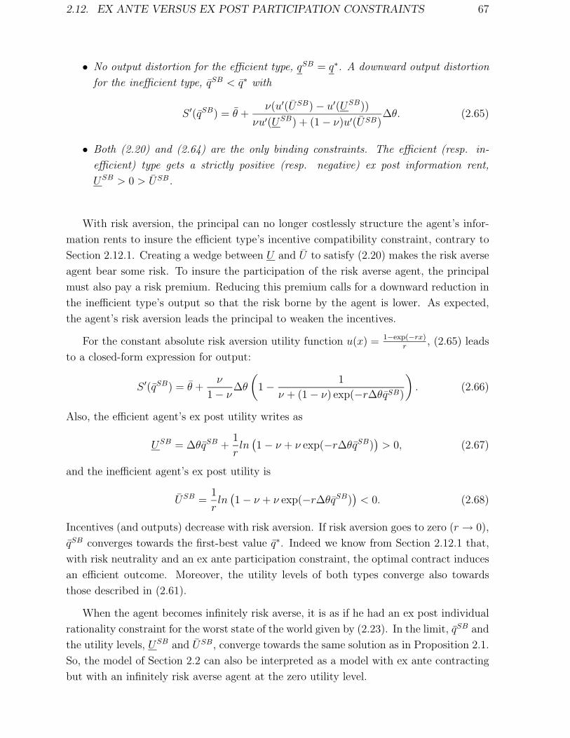
2.12. EX ANTE VERSUS EX POST PARTICIPATION CONSTRAINTS 67
• No output distortion for the efficient type, qSB = q∗. A downward output distortion
for the inefficient type, qSB < q∗ with
S ′(qSB) = θ +ν(u′(USB)− u′(USB))
νu′(USB) + (1− ν)u′(USB)∆θ. (2.65)
• Both (2.20) and (2.64) are the only binding constraints. The efficient (resp. in-
efficient) type gets a strictly positive (resp. negative) ex post information rent,
USB > 0 > USB.
With risk aversion, the principal can no longer costlessly structure the agent’s infor-
mation rents to insure the efficient type’s incentive compatibility constraint, contrary to
Section 2.12.1. Creating a wedge between U and U to satisfy (2.20) makes the risk averse
agent bear some risk. To insure the participation of the risk averse agent, the principal
must also pay a risk premium. Reducing this premium calls for a downward reduction in
the inefficient type’s output so that the risk borne by the agent is lower. As expected,
the agent’s risk aversion leads the principal to weaken the incentives.
For the constant absolute risk aversion utility function u(x) = 1−exp(−rx)r
, (2.65) leads
to a closed-form expression for output:
S ′(qSB) = θ +ν
1− ν∆θ
(1− 1
ν + (1− ν) exp(−r∆θqSB)
). (2.66)
Also, the efficient agent’s ex post utility writes as
USB = ∆θqSB +1
rln
(1− ν + ν exp(−r∆θqSB)
)> 0, (2.67)
and the inefficient agent’s ex post utility is
USB =1
rln
(1− ν + ν exp(−r∆θqSB)
)< 0. (2.68)
Incentives (and outputs) decrease with risk aversion. If risk aversion goes to zero (r → 0),
qSB converges towards the first-best value q∗. Indeed we know from Section 2.12.1 that,
with risk neutrality and an ex ante participation constraint, the optimal contract induces
an efficient outcome. Moreover, the utility levels of both types converge also towards
those described in (2.61).
When the agent becomes infinitely risk averse, it is as if he had an ex post individual
rationality constraint for the worst state of the world given by (2.23). In the limit, qSB and
the utility levels, USB and USB, converge towards the same solution as in Proposition 2.1.
So, the model of Section 2.2 can also be interpreted as a model with ex ante contracting
but with an infinitely risk averse agent at the zero utility level.

68 CHAPTER 2. THE RENT EXTRACTION-EFFICIENCY TRADE-OFF
Salanie (1990) analyzed the case of a continuum of types. Pooling for the least
efficient types occurs when risk aversion is large enough. Laffont and Rochet (1998)
showed a similar phenomenon with ex post participation constraints when a regulator
(the principal) maximizes ex ante social welfare with a risk averse firm.
A Risk Averse Principal
Consider now a risk averse principal with utility function v(·) defined on his gains from
trade S(q) − t such that v′(·) > 0, v′′(·) < 0 and v(0) = 0. Again, the contract between
the principal and the risk neutral agent is signed before the agent knows his type.
In this context, the first-best contract obviously calls for the first-best output q∗ and
q∗ being produced. It also calls for the principal being fully insured between both states
of nature and for the agent’s ex ante participation constraint being binding. This leads
us to the following two conditions which must be satisfied by the agent’s rents U∗ and
U∗:
S(q∗)− θq∗ − U∗ = S(q∗)− θq∗ − U∗, (2.69)
and
νU∗ + (1− ν)U∗ = 0. (2.70)
Solving, this system of two equations with two unknowns (U∗, U∗) yields:
U∗ = (1− ν)(S(q∗)− θq∗ − (S(q∗)− θq∗)
), (2.71)
and
U∗ = −ν(S(q∗)− θq∗ − (S(q∗)− θq∗)
). (2.72)
Note that the first-best profile of information rents satisfies both types’ incentive
compatibility constraints since:
U∗ − U∗ = S(q∗)− θq∗ − (S(q∗)− θq∗) > ∆θq∗ (2.73)
(from the definition of q∗) and
U∗ − U∗ = S(q∗)− θq∗ − (S(q∗)− θq∗) > −∆θq∗, (2.74)
(from the definition of q∗). Henceforth, the profile of rents (U∗, U∗) is incentive compatible
and the first-best allocation is easily implemented in this framework.

2.12. EX ANTE VERSUS EX POST PARTICIPATION CONSTRAINTS 69
Proposition 2.5 : When the principal is risk averse over the monetary gains S(q) − t
and contracting takes place ex ante, the optimal incentive feasible contract implements the
first-best outcome.
It is interesting to note that U∗ and U∗ obtained in (2.71) and (2.72) are also the levels
of rent obtained in (2.62) and (2.63). Indeed, the lump-sum payment T = ν(S(q∗)−θq∗)+(1− ν)(S(q∗)− θq∗) which allows the principal to make the risk neutral agent’s residual
claimant for the hierarchy’s profit provides also full insurance to the principal.
By making the risk neutral agent residual claimant for the value of trade, ex ante
contracting allows the risk averse principal to implement the first-best outcome despite
the informational problem.
Of course this result does not hold anymore if the agent’s ex post participation con-
straint must be satisfied. In this case, we still guess a solution such that (2.21) is slack at
the optimum. The principal’s program reduces now to:
(P ) : max{(U ,q),(U,q)}
νv(S(q)− θq − U
)+ (1− ν)v
(S(q)− θq − U
)subject to (2.20) and (2.23).
Inserting the values of U and U obtained from the binding constraints (2.20) and
(2.23) into the principal’s objective function and optimizing with respect to outputs leads
to qSB = q∗, i.e., no distortion for the efficient type just as in the case of risk neutrality
and a downward distortion of the inefficient type’s output qSB < q∗ given by
S ′(qSB) = θ +νv′(V SB)
(1− ν)v′(V SB)∆θ, (2.75)
where V SB = S(q∗)−θq∗−∆θqSB and V SB = S(qSB)− θqSB are the principal’s payoffs in
both states of nature. We can check that V SB < V SB since S(qSB)− θqSB < S(q∗)− θq∗
from the definition of q∗. In particular, we observe that the distortion in the right-hand
side of (2.75) is always lower than ν1−ν
∆θ, its value with a risk neutral principal. The
intuition is straightforward. By increasing q above its value with risk neutrality, the
risk averse principal reduces the difference between V SB and V SB. This gives him some
insurance and increases his ex ante payoff.
Risk aversion on the side of the principal is quite natural in some contexts. A local
regulator with a limited budget or a specialized bank dealing with relatively correlated
projects may be insufficiently diversified to become completely risk neutral. See Lewis
and Sappington (1995) for some application to the regulation of public utilities.

70 CHAPTER 2. THE RENT EXTRACTION-EFFICIENCY TRADE-OFF
2.13 Commitment
To solve our incentive problem, we have implicitly assumed that the principal has a
strong ability to commit himself to a distribution of rents inducing information revelation,
but also to some allocative inefficiency designed at reducing the cost of this revelation.
Alternatively, this assumption also means that the Court of Justice can perfectly enforce
the contract and that neither renegotiating nor reneging on the contract is a feasible
alternative for the agent or (and) the principal. What could happen when any of those
two assumptions is relaxed?
2.13.1 Renegotiating a Contract
A first source of limited commitment occurs when the principal can renegotiate the con-
tract offer to the agent along the course of actions. Renegotiation is a voluntary act which
should benefit both the principal and the agent. It should be contrasted with a breach of
contract which can hurt one of the contracting parties. On the contrary, one should view
a renegotiation procedure as the ability of the contracting partners to achieve a Pareto
improvement trade if any becomes incentive feasible along the course of actions.
Indeed, once the different types have revealed themselves to the principal by selecting
respectively the contracts (tSB, qSB) for the efficient type and (tSB, qSB) for the inefficient
type, the principal may propose a renegotiation to get around the allocative inefficiency
he has imposed on the inefficient agent’s output. The gain from this renegotiation comes
from raising allocative efficiency for the inefficient type and moving output from qSB to
q∗. To share these new gains from trade with the inefficient agent, the principal must at
least offer him the same utility level as before renegotiation. The participation constraint
of the inefficient agent can still be kept at zero when the transfer of this type is raised
from tSB = θqSB to t∗ = θq∗. However, raising this transfer also hardens the incentive
compatibility constraint of the efficient type. Indeed, it becomes more valuable for an
efficient type to hide his type to obtain this larger transfer, and truthful revelation by
the efficient type is no longer obtained in equilibrium. There is a fundamental trade-off
between raising efficiency ex post and hardening ex ante incentives when renegotiation is
an issue.
The ability to commit to a menu of contracts may not be too problematic in some
instances. Producing a quantity q may require to build a capacity up to that level.22
Raising production as requested by the renegotiation procedure asks for increasing the
productive capacity and this can be excessively costly compared to the allocative gains
coming from a larger volume of trade. Moreover, this commitment issue seems highly
22See Beaudry and Poitevin (1994) for a model along these lines.

2.14. STOCHASTIC MECHANISMS 71
dependent on the use of a direct revelation mechanism since renegotiation takes place
after the agent has revealed his type, but before the principal imposes an output target.
Let us thus consider the simple and equivalent indirect mechanism where the principal
offers the same menu to the agent, but let the agent choose the output himself (as we have
done in the beginning of this chapter). This alternative mechanism does not require any
communication from the agent to the principal before production takes place. The agent
is delegated the choice of an output and, once this choice is made, there is no scope for
renegotiation since the one-shot relationship ends. The commitment issue becomes much
more problematic in truly dynamic contexts where different actions take place at various
dates. We will return to the difficult issues raised by the renegotiation of contracts in
Chapter 9 and Volume III.
2.13.2 Reneging on a Contract
A second source of imperfection arises when either the principal or the agent may breach
the contract and thus renege on his previous contractual obligation. Let us take the
case of the principal reneging the contract.23 Indeed, once the agent has revealed himself
to the principal by selecting the contract within the menu offered by the principal, the
latter, having learned the agent’s type, may propose the complete information contract
which extracts all rents without inducing any allocative efficiency. Of course, this breach
of contract should be anticipated by the agent and these anticipations will interfer with
truthful revelation in the first place. Also, the agent may want to renege on a contract
which gives him a negative ex post utility level as we mentioned in Section 2.12.1. In
this case, the threat of the agent reneging a contract signed at the ex ante stage forces
the agent’s participation to be written in ex post terms. Such a setting justifies also the
focus of this chapter on the case of interim contracting. In Chapter 9, we will also discuss
further the issue of enforcement.
2.14 Stochastic Mechanisms
We consider here the framework of Section 2.11 with a general cost function C(q, θ). Let
us rewrite the principal’s problem as:
(P ) : max{(q,U);(q,U)}
ν(S(q)− C(q, θ)
)+ (1− ν)
(S(q)− C(q, θ)
)− νU − (1− ν)U ,
subject to
23See Section 8.4.3 and Section 9.2 for other models where the agent may renege on the contract.
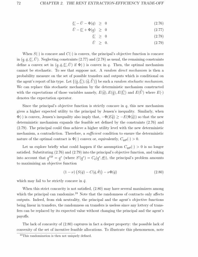
72 CHAPTER 2. THE RENT EXTRACTION-EFFICIENCY TRADE-OFF
U − U − Φ(q) ≥ 0 (2.76)
U − U + Φ(q) ≥ 0 (2.77)
U ≥ 0 (2.78)
U ≥ 0. (2.79)
When S(·) is concave and C(·) is convex, the principal’s objective function is concave
in (q, q, U, U). Neglecting constraints (2.77) and (2.78) as usual, the remaining constraints
define a convex set in (q, q, U, U) if Φ(·) is convex in q. Then, the optimal mechanism
cannot be stochastic. To see that suppose not. A random direct mechanism is then a
probability measure on the set of possible transfers and outputs which is conditional on
the agent’s report of his type. Let {(q, U); (˜q, ˜U)} be such a random stochastic mechanism.
We can replace this stochastic mechanism by the deterministic mechanism constructed
with the expectations of those variables namely, E(˜q), E(q), E(U) and E( ˜U) where E(·)denotes the expectation operator.
Since the principal’s objective function is strictly concave in q, this new mechanism
gives a higher expected utility to the principal by Jensen’s inequality. Similarly, when
Φ(·) is convex, Jensen’s inequality also imply that, −Φ(E˜q) ≥ −E(Φ(˜q)) so that the new
deterministic mechanism expands the feasible set defined by the constraints (2.76) and
(2.79). The principal could thus achieve a higher utility level with the new deterministic
mechanism, a contradiction. Therefore, a sufficient condition to ensure the deterministic
nature of the optimal contract is Φ(·) convex or, equivalently, Cqqθ(·) > 0.
Let us explore briefly what could happen if the assumption Cqqθ(·) > 0 is no longer
satisfied. Substituting (2.76) and (2.79) into the principal’s objective function, and taking
into account that qSB = q∗ (where S ′(q∗) = Cq(q∗, θ)), the principal’s problem amounts
to maximizing an objective function
(1− ν)(S(q)− C(q, θ)
)− νΦ(q) (2.80)
which may fail to be strictly concave in q.
When this strict concavity is not satisfied, (2.80) may have several maximizers among
which the principal can randomize.24 Note that the randomness of contracts only affects
outputs. Indeed, from risk neutrality, the principal and the agent’s objective functions
being linear in transfers, the randomness on transfers is useless since any lottery of trans-
fers can be replaced by its expected value without changing the principal and the agent’s
payoffs.
The lack of concavity of (2.80) captures in fact a deeper property: the possible lack of
convexity of the set of incentive feasible allocations. To illustrate this phenomenon, note24This randomization is then not uniquely defined.
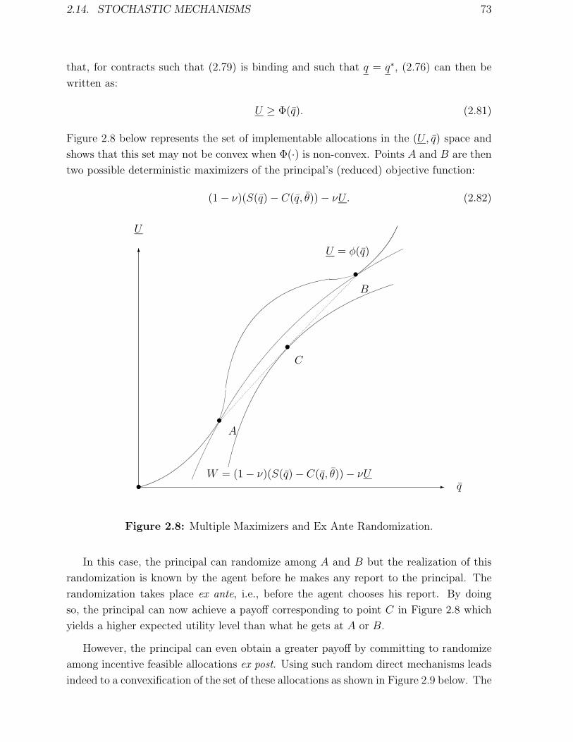
2.14. STOCHASTIC MECHANISMS 73
that, for contracts such that (2.79) is binding and such that q = q∗, (2.76) can then be
written as:
U ≥ Φ(q). (2.81)
Figure 2.8 below represents the set of implementable allocations in the (U, q) space and
shows that this set may not be convex when Φ(·) is non-convex. Points A and B are then
two possible deterministic maximizers of the principal’s (reduced) objective function:
(1− ν)(S(q)− C(q, θ))− νU. (2.82)
-
6
U
q•
•
•U = φ(q)
B
A
W = (1− ν)(S(q)− C(q, θ))− νU
•C
Figure 2.8: Multiple Maximizers and Ex Ante Randomization.
In this case, the principal can randomize among A and B but the realization of this
randomization is known by the agent before he makes any report to the principal. The
randomization takes place ex ante, i.e., before the agent chooses his report. By doing
so, the principal can now achieve a payoff corresponding to point C in Figure 2.8 which
yields a higher expected utility level than what he gets at A or B.
However, the principal can even obtain a greater payoff by committing to randomize
among incentive feasible allocations ex post. Using such random direct mechanisms leads
indeed to a convexification of the set of these allocations as shown in Figure 2.9 below. The

74 CHAPTER 2. THE RENT EXTRACTION-EFFICIENCY TRADE-OFF
objective function (2.82) being strictly convex in (U, q), there exists a unique maximizer
to the principal’s problem and it is now described by point D.
-
6
U
q
¡¡
¡¡
¡¡
¡¡
¡¡
¡¡
¡¡
¡¡
¡¡
¡¡¡
•
•B
•A
D•C
Convexification
@@
@@@R
Figure 2.9: Unique Maximizer and Ex Post Randomization.
By being able to commit to an ex post randomization through a stochastic mechanism,
the principal can achieve a payoff which is strictly greater than what he obtains with
deterministic mechanisms or with an ex ante randomization. Of course, the difficulty
may come from the fact that this randomization has to be verifiable by a Court of Justice
to be contracted upon. Ensuring this verifiability is a slightly more difficult problem than
ensuring that a deterministic mechanism is enforced since any deviation away from a given
randomization can only be statistically detected once sufficiently many realizations of the
contracts have been observed. This suggests that such a deviation can only be detected
in a repeated relationship framework or when the principal is involved in many bilateral
one-shot principal-agent relationships. The enforcement of such stochastic mechanisms is
thus particularly problematic. This has led scholars to give up those random mechanisms
or, at least, to focus on economic settings where they are not optimal.
Stochastic mechanisms have been sometimes suggested in the insurance, the
nonlinear pricing and optimal taxation literatures (see Stiglitz (1987), Arnott and Stiglitz
(1988)) as well as in the price discrimination literature (see Maskin and Riley (1984) and
Moore (1985)).

2.15. INFORMATIVE SIGNALS TO IMPROVE CONTRACTING 75
2.15 Informative Signals to Improve Contracting
In this section, we investigate the impacts of various improvements of the principal’s infor-
mation system on the optimal contract. The idea here is to see how pieces of information
exogenous to the relationship can help the principal to design the contract with the agent.
The simple observation of performances in similar principal-agent relationships and the
setting up of monitoring and auditing structures which are specific to the relationship
are all informational devices used to improve the agent’s control by somewhat filling the
information gap between the principal and his agent.
2.15.1 Ex Post Verifiable Signal
Suppose that the principal, the agent and the Court of Justice observe ex post a verifiable
signal σ which is correlated with θ. This signal is observed after the agent’s choice of
production (or alternatively after the agent’s report to the principal in a direct revelation
mechanism). The contract can then be conditioned on both the agent’s report and the
observed signal which provides useful information on the underlying state of nature.
For simplicity, we assume that this signal may take only two values σ1 and σ2. Let
the conditional probabilities of these respective realizations of the signal be µ1 = Pr(σ =
σ1/θ = θ) ≥ 1/2 and µ2 = Pr(σ = σ2/θ = θ) ≥ 1/2. Note that, if µ1 = µ2 = 1/2, the
signal σ is uninformative. Otherwise, σ1 brings “good news” on the fact that the agent
is efficient and σ2 brings “bad news” since it is more likely that the agent is inefficient in
this case.
Let us adopt the following notations for the information rents u11 = t(θ, σ1)−θq(θ, σ1),
u12 = t(θ, σ2)− θq(θ, σ2), u21 = t(θ, σ1)− θq(θ, σ1) and u22 = t(θ, σ2)− θq(θ, σ2). Similar
notations are used for the outputs qij. The agent knows his type before the signal σ
realizes. Then, the incentive and participation constraints must be written in expectation
over the realization of σ. Incentive constraints for both types write respectively as:
µ1u11 + (1− µ1)u12 ≥ µ1(u21 + ∆θq21) + (1− µ1)(u22 + ∆θq22), (2.83)
(1− µ2)u21 + µ2u22 ≥ (1− µ2)(u11 −∆θq11) + µ2(u12 −∆θq12). (2.84)
The contract being accepted by each type after learning his type but before the realization
of the signal, participation constraints for both types write as:
µ1u11 + (1− µ1)u12 ≥ 0, (2.85)
(1− µ2)u21 + µ2u22 ≥ 0. (2.86)

76 CHAPTER 2. THE RENT EXTRACTION-EFFICIENCY TRADE-OFF
Note that, for a given schedule of output qij, the system (2.83) to (2.86) has as many
equations as unknowns uij. When the determinant of the system (2.83) to (2.86) is non-
zero, it is possible to find ex post rents uij (or equivalently transfers) such that all these
constraints are binding.25 In this case, the agent receives no rent whatever his type.
Moreover, any choice of production levels, in particular the complete information optimal
ones, can be implemented this way. The determinant of the system is non-zero when:
1− µ1 − µ2 6= 0. (2.87)
Importantly, condition (2.87) holds generically. It fails only if µ1 + µ2 = 1 which corre-
sponds to the case of a uninformative signal.
Riordan and Sappington (1988) were the first to introduce the condition (2.87).
Cremer and McLean (1988) generalized this use of correlated information in their analysis
of multi-agent models. These authors use another mathematical tool to ensure that
incentive constraints are slack: Farkas’ Lemma. We will cover this important topic for
incentive theory with multiple agents in Volume II.
2.15.2 Ex Ante Nonverifiable Signal
We keep the same informational structure as in Section 2.15.1, but we suppose now that
a nonverifiable binary signal σ about θ is available to the principal at the ex ante stage.
Before offering an incentive contract, the principal computes for each value of this signal
his posterior belief that the agent is efficient, namely:
ν1 = Pr(θ = θ/σ = σ1) =νµ1
νµ1 + (1− ν)(1− µ2)(2.88)
ν2 = Pr(θ = θ/σ = σ2) =ν(1− µ1)
ν(1− µ1) + (1− ν)µ2
. (2.89)
Then, the optimal contract entails a downward distortion of the inefficient agent’s pro-
duction qSB(σi) which is, for signals σ1 and σ2 respectively:
S ′(qSB(σ1)) = θ +ν1
1− ν1
∆θ = θ +νµ1
(1− ν)(1− µ2)∆θ, (2.90)
S ′(qSB(σ2)) = θ +ν2
1− ν2
∆θ = θ +ν(1− µ1)
(1− ν)µ2
∆θ. (2.91)
In the case where µ1 = µ2 = µ > 12, we can interpret µ as an index of the informativeness
of the signal. Observing σ1, the principal thinks that it is more likely that the agent is
25In fact, using Farkas’ lemma, one can even ensure that incentive constraints are strict inequalities.

2.15. INFORMATIVE SIGNALS TO IMPROVE CONTRACTING 77
efficient. A stronger reduction in the efficient type’s information rent is called for after
σ1. (2.90) shows that incentives decrease with respect to the case without informative
signal since ( µ1
1−µ2> 1). In particular, if µ2 is large enough, the principal shuts down
the inefficient firm after having observed σ1. He offers a high powered incentive contract
to the efficient agent only which leaves him no rent. On the contrary, because it is less
likely to face an efficient type after having observed σ2, the principal reduces less the
information rent than in the case without informative signal since (1−µ1
µ2< 1). Incentives
are stronger.
See Boyer and Laffont (2000) for a comparative statics analysis of the effect of
a more competitive environment on the optimal contract. In their analysis, the competi-
tiveness of the environment is linked to the informativeness of the signal σ.
2.15.3 More or Less Favorable Distribution of Types
In the last two Sections 2.15.1 and 2.15.2, the principal benefits from improvements in
the information structure. More generally, even in the basic model of this chapter, one
may wonder how information structures can be ranked by the principal and the agent.
We will say that a distribution (ν, 1− ν) is more favorable than a distribution (ν, 1−ν)
if and only if ν > ν. Then, the expected utility of the principal is higher with a more
favorable distribution. Indeed, we can define this expected utility as:
V (ν) = ν(S(q∗)− θq∗ −∆θqSB(ν)) + (1− ν)(S(qSB(ν))− θqSB), (2.92)
where we make explicit the dependence of V and qSB on ν.
Using the Envelope Theorem, we obtain:
dV (ν)
dν= (S(q∗)− θq∗ −∆θqSB)− (S(qSB)− θqSB)
= (S(q∗)− θq∗)− (S(qSB)− θqSB), (2.93)
which is strictly positive by definition of q∗.
The rent of the efficient type, ∆θqSB, is clearly lower when the distribution is more
favorable. Indeed, as it can be seen on (2.28), qSB(ν) is a decreasing function of ν. So,
incentives decrease as the distribution becomes more favorable. Indeed, the perspective
of a more likely efficient type leads the principal to a trade-off which is tilted against
information rents, i.e., a trade-off which is less favorable to allocative efficiency. For the
ex ante rent of the agent, U(ν) = ν∆θqSB(ν), we have instead:
dU(ν)
dν= ∆θqSB(ν) + ν∆θ
dqSB(ν)
dν(2.94)

78 CHAPTER 2. THE RENT EXTRACTION-EFFICIENCY TRADE-OFF
or, using (2.28),
dU(ν)
dν= ∆θqSB(ν)︸ ︷︷ ︸
>0
+ν(∆θ)2
(1− ν)2S ′′(qSB)︸ ︷︷ ︸<0
(ν). (2.95)
Therefore, for ∆θ small enough the expected rent increases when the distribution is
more favorable but it decreases when ∆θ is rather large. Note that, if there is shut-down
when ν becomes larger, the expected rent decreases necessarily. The most interesting
result is thus that, for ∆θ small, both the principal and the agent gain from a more
favorable distribution. There is no conflict of interests on the choice of the information
structure.
See Laffont and Tirole (1993, Chapter 1) for a similar analysis in the case of a
continuum of types.
2.16 Contract Theory at Work
This section proposes several classical settings where the basic model of this chapter is
useful. Introducing adverse selection in each of these contexts has proved to be a quite
significative improvement of standard microeconomic analysis.
2.16.1 Regulation
In the Baron and Myerson (1982) regulation model, the principal is a regulator who max-
imizes a weighted average of the consumers’ surplus S(q)− t and a regulated monopoly’s
profit U = t − θq with a weight α less than one for the firm’s profit. The principal’s
objective function writes now as V = S(q)− θq− (1−α)U . Because α is less than one, it
is again socially costly to give up a rent to the firm. Maximizing expected social welfare
under incentive and participation constraints leads to qSB = q∗ for the efficient type and
to a downward distortion for the inefficient type which is given by:
S ′(qSB) = θ +ν
1− ν(1− α)∆θ. (2.96)
Note that a higher value of α reduces the output distortion since the regulator is less
concerned by the distribution of rents within society as α increases.
The regulation literature of the last fifteen years has improved greatly our under-
standing of government intervention under asymmetric information. We refer to Laffont
and Tirole (1993) for a comprehensive view of this theory and its various implications for
the design of real world regulatory institutions.

2.16. CONTRACT THEORY AT WORK 79
2.16.2 Nonlinear Pricing of a Monopoly
In Maskin and Riley (1984), the principal is the seller of a private good with production
cost cq who faces a continuum of buyers. The principal has thus a utility function V =
t − cq. The tastes of a buyer for the private good are such that his utility function is
U = θu(q) − t where q is the quantity consumed and t his payment to the principal. As
in our analysis of Section 2.6, one can view the parameter θ of each buyer as being drawn
independently from the same distribution26 on Θ = {θ, θ} with respective probabilities
1− ν and ν.
Incentive and participation constraints can, as usual, be written directly in terms of
the information rents U = θu(q)− t and U = θu(q)− t as:
U ≥ U −∆θu(q), (2.97)
U ≥ U + ∆θu(q), (2.98)
U ≥ 0, (2.99)
U ≥ 0. (2.100)
The principal’s program takes now the following form:
(P ) : max{(U ,q),(U,q)}
ν(θu(q)− cq
)+ (1− ν)
(θu(q)− cq
)− (νU + (1− ν)U
)subject to (2.97) to (2.100).
The analysis is the mirror image of that of Section 2.6 since now the “efficient type” is
the one with the highest valuation for the good θ. Hence, (2.98) and (2.99) are the two
binding constraints. As a result, there is no output distortion with respect to the first-best
outcome for the high valuation type and qSB = q∗ where
θu′(q∗) = c. (2.101)
However, there exists a downward distortion of the low valuation agent’s output with
respect to the first-best outcome. We have qSB < q∗ where(θ − ν
1− ν∆θ
)u′(qSB) = c. (2.102)
26Note that this distribution is now the actual distribution of types (i.e., ν is the frequency of type θby the Law of Large Numbers), and not a probability distribution. This interpretation also applies tothe basic model of this chapter and enlarges considerably its relevance.

80 CHAPTER 2. THE RENT EXTRACTION-EFFICIENCY TRADE-OFF
and θu′(q∗) = c.
The literature on nonlinear pricing is huge. The interested reader will find in
Tirole (1988), Varian (1988) and Wilson (1993) excellent reviews of this topic. In Chapter
9, we discuss the link between direct revelation mechanisms and nonlinear prices, and in
particular how and when the optimal direct mechanism can be implemented with a menu
of linear prices.
2.16.3 Quality and Price Discrimination
Mussa and Rosen (1978) have studied a very similar problem as in Section 2.16.2 where
agents buy one unit of a commodity with quality q but are vertically differentiated with
respect to their preferences for the good. The marginal cost (and average cost) of produc-
ing one unit of quality q is C(q) and the principal has the utility function V = t− C(q).
The utility function of an agent is now U = θq − t with θ in Θ = {θ, θ} with respective
probabilities 1− ν and ν.
Incentive and participation constraints can still be written directly in terms of the
information rents U = θq − t and U = θq − t as:
U ≥ U −∆θq, (2.103)
U ≥ U + ∆θq, (2.104)
U ≥ 0, (2.105)
U ≥ 0. (2.106)
The principal solves now:
(P ) : max{(U,q),(U ,q)}
ν(θq − C(q)
)+ (1− ν)
(θq − C(q)
)− (νU + (1− ν)U
)subject to (2.103) to (2.106).
Following similar procedures to what we have done so far, only (2.104) to (2.105) are
binding constraints. Finally, we find that the high valuation agent receives the first-best
quality qSB = q∗ where θ = C ′(q∗). However, quality is now reduced below the first-best
for the low valuation agent. We have qSB < q∗ where:
θ = C ′(qSB) +ν
1− ν∆θ. (2.107)

2.16. CONTRACT THEORY AT WORK 81
Interestingly, the spectrum of qualities (defined as the difference of qualities between what
is obtained respectively by the high valuation and by the low valuation agent) is larger
under asymmetric information than under complete information. This incentive of the
seller to put a low quality good on the market is a well documented phenomenon in the
industrial organization literature. Some authors have even argued that damaging its own
goods may be part of the firm’s optimal selling strategy when screening of the consumers’
willingness to pay for quality is an important issue.27
2.16.4 Financial Contracts
Asymmetric information affects significantly the financial markets. For instance, in Freixas
and Laffont (1990), the principal is a lender who provides a loan with size k to a bor-
rower. Capital costs Rk to the lender since it could be invested elsewhere in the economy
to earn the risk free interest rate R. The lender has thus a utility function V = t − Rk.
The borrower makes a profit V = θf(k) − t where f(k) is the return on capital and t is
the borrower’s repayment to the lender. We assume that f ′(·) > 0 and f ′′(·) < 0. The
parameter θ is a productivity shock drawn from Θ = {θ, θ} with respective probabilities
1− ν and ν.
Incentive and participation constraints can again be written directly in terms of the
information rents U = θf(k)− t and U = θf(k)− t as
U ≥ U −∆θf(k), (2.108)
U ≥ U + ∆θf(k), (2.109)
U ≥ 0, (2.110)
U ≥ 0. (2.111)
The principal’s program takes now the following form:
(P ) : max{(U,k);(U ,k)}
ν(θf(k)−Rk
)+ (1− ν) (θf(k)−Rk)− (
νU + (1− ν)U)
subject to (2.108) to (2.111).
We let the reader check that (2.109) and (2.110) are now the two binding constraints. As
a result, there is no capital distortion with respect to the first-best outcome for the high
productivity type and kSB = k∗ where θf ′(k∗) = R. In this case, the return on capital
27Edgeworth (1857).

82 CHAPTER 2. THE RENT EXTRACTION-EFFICIENCY TRADE-OFF
is equal to the risk free interest rate. However, there exists also a downward distortion
of the low productivity borrower’s loan with respect to the first-best outcome. We have
kSB < k∗ where (θ − ν
1− ν∆θ
)f ′(kSB) = R. (2.112)
and θf ′(k∗) = R.
Screening borrowers according to the size of their loans amounts to some kind of ra-
tioning for the low productivity firms. This phenomenon is well documented in the finance
literature and we refer to Freixas and Rochet (1999, Chapter 5) for further references.
We will see in Section 3.7 that the lender may also rely on other screening devices,
like auditing or the threat of termination, to get valuable information on the firm.
2.16.5 Labor Contracts
Asymmetric information undermines also the relationship between a worker and the firm
for which he works. In Green and Khan (1983) and Hart (1983) among others, the
principal is a union (or a set of workers) who provides its labor force l to a firm. To
simplify the analysis, we assume that it has full bargaining power in determining the
labor contract with the firm and the latter has a zero reservation utility.
The firm makes a profit θf(l)−t where f(l) is the return on labor and t is the worker’s
payment. We assume that f ′(·) > 0 and f ′′(·) < 0. The parameter θ is a productivity
shock drawn from Θ = {θ, θ} with respective probabilities 1 − ν and ν. In the labor
contracting literature, the firm knows the realization of the shock and the union ignores
its value. The firm is objective is to maximize its profit U = θf(`) − t. Workers have a
utility function defined on consumption and labor. If their disutility of labor is counted in
monetary terms and all payments from the firm are consumed, they get V = v(t− ψ(l))
where ψ(·) is their disutility of labor which is increasing and convex (ψ′(·) > 0, ψ′′(·) > 0)
and v(·) is increasing and concave (v′(·) > 0, v′′(·) < 0).
In this context, the firm’s boundaries are determined before the realization of the
shock and contracting takes place ex ante. The firm’s ex ante participation constraint
writes thus as (2.70). It should thus be also clear that the model is completely isomorphic
to that of Section 2.13.2 with a risk averse principal and a risk neutral agent.
Using the results above, we know that the risk averse union will propose a contract to
the risk neutral firm which provides full insurance and implements the first-best levels of
employments ¯∗ and `∗ defined respectively by θf ′(¯∗) = ψ′(¯∗) and θf ′(`∗) = ψ′(`∗).
Let us now turn to the more difficult case where workers have a utility function ex-

2.16. CONTRACT THEORY AT WORK 83
hibiting an income effect and let us assume, to simplify, that V = v(t)− ψ(`).
The first-best optimal contract would still require efficient employment in both states
of nature. Moreover, it would also call for equating the worker’s marginal utility of income
across states:
t∗ = t∗, (2.113)
and making the firm’s expected utility equal to zero
ν(θf(¯∗)− t∗) + (1− ν)(θf(`∗)− t∗) = 0. (2.114)
Solving those latter two equations for the pair of transfers (t∗, t∗) immediately yields
t∗ = t∗ = νθf(¯∗) + (1 − ν)θf(`∗) = E(θf(`∗)), where E(·) denotes the expectation
operator with respect to θ.
Inserting this value of the transfer into the union’s objective function, the principal
chooses levels of employment which are obtained as solutions to:
(P ) : max{(¯,`)}
v(νθf(¯) + (1− ν)θf(`)
)− νψ(¯)− (1− ν)ψ(`).
We immediately find the first-best levels of labor:
θf ′(¯∗) =ψ′(¯∗)
v′(E(θf(`∗))), (2.115)
and
θf ′(`∗) =ψ′(`∗)
v′(E(θf(`∗))). (2.116)
It follows that θ f ′(¯∗)ψ′(¯) = θ f ′(`∗)
ψ′(`∗) and thus, using the fact that f ′ψ′ is decreasing, we obtain
that ¯∗ > `∗.
Let us now consider the case of asymmetric information. The firm’s incentive com-
patibility constraints in both states of nature write as:
U − U ≥ ∆θf(`) (2.117)
in the good state θ, and
U − U ≥ −∆θf(¯) (2.118)
in the bad state θ.
Note that the first-best levels of information rents U∗ = θf(`∗)−t∗ and U∗ = θf(¯∗)−t∗
satisfy (2.117) but violate (2.118). Henceforth, let us look for an optimal incentive feasible

84 CHAPTER 2. THE RENT EXTRACTION-EFFICIENCY TRADE-OFF
contract where the binding incentive constraint prevents the firm from claiming that a
high shock θ has realized when, in fact, a low shock θ has realized. The union’s problem
writes thus as:
(P ) : max{(U ,¯);(U,`)}
ν(v(θf(¯)− U)− ψ(¯)
)+ (1− ν) (v(θf(`)− U)− ψ(`))
subject to (2.118) and
νU + (1− ν)U ≥ 0. (2.119)
We let the reader check that both constraints above are binding at the optimum. In
this case, we have U = (1 − ν)∆θf(¯) and U = −ν∆θf(¯). Inserting those expressions
of the firm’s information rents into the union’s objective function and optimizing with
respect to ¯ and ` yields:
θf ′(`SB) =ψ′(`SB)
v′(V SB)(2.120)
and (θ − (1− ν)∆θ(v′(V SB)− v′(V SB))
v′(V SB)
)f ′(¯SB) =
ψ′(¯SB)
v′(V SB), (2.121)
where V SB = θf(¯SB)− (1− ν)∆θf(¯SB) and V SB = θf(`SB) + ν∆θf(¯SB).
Note that V SB > V SB as long as the implementability condition ¯SB > `SB is satisfied.
The virtual shock ˜θ and the true shock θ in the good state of nature are such that
˜θ = θ − (1− ν)∆θ(v′(V SB)− v′(V SB))
v′(V SB)> θ. (2.122)
Therefore, as it can seen by comparing (2.115) and (2.121), asymmetric information
creates an incentive for the union to expand output over the first-best level ¯∗.
This optimal overemployment has often been critized in the labor literature as
coming from the fact that the worker’s utility function used in our example is such that
labor is a normal good. For more general preferences, underemployment can instead be
obtained as an optimal solution to the asymmetric information problem. For further
references on this topic, the interested reader can look at Hart and Holmstrom (1987)
and Blanchard and Fisher (1989, Chapter 9) and references therein.

2.16. CONTRACT THEORY AT WORK 85
APPENDIX 2.1: The Continuum of Types
Despite the fact that few new economic insights can be obtained in the continuum
case, we give in this appendix a brief account of this case because most of the literature
is written within this framework.
Reconsider the model of Section 2.2 with θ in Θ = [θ, θ], with a cumulative distribution
function F (θ) and a density function f(θ) > 0 on [θ, θ]. The Revelation Principle is still
valid in this context and we can restrict our analysis to direct revelation mechanisms
{(q(θ), t(θ))} which are truthful, i.e., here such that:
t(θ)− θq(θ) ≥ t(θ)− θq(θ) for any (θ, θ) in Θ2. (2.123)
In particular (2.123) implies:
t(θ)− θq(θ) ≥ t(θ′)− θq(θ′), (2.124)
t(θ′)− θ′q(θ′) ≥ t(θ)− θ′q(θ) for all pairs (θ, θ′) in Θ2. (2.125)
Adding (2.124) and (2.125) we obtain:
(θ − θ′)(q(θ′)− q(θ)) ≥ 0. (2.126)
Incentive compatibility alone requires that the schedule of output q(·) has to be non
increasing. This implies that q(·) is differentiable almost everywhere (a.e.), from which
we can derive that t(·) is also differentiable with the same points of non-differentiability.
The most general class of direct revelation mechanisms to consider is therefore the class
of a.e. differentiable functions. In practice, we use piecewise differentiable functions and
in most cases differentiable functions. Here, we will restrict the analysis to differentiable
functions, but it can be immediately extended to piecewise differentiable functions28
(2.123) implies the following first-order condition for the optimal response θ chosen by
type θ is satisfied:
dt
dθ(θ)− θ
dq
dθ(θ) = 0. (2.127)
For the truth to be an optimal response for all θ, it must be the case that
dt
dθ(θ)− θ
dq(θ)
dθ= 0, (2.128)
and (2.128) must hold for all θ in Θ since θ is unknown to the principal.
28See Laffont and Tirole (1993, Chapter 6) for an example of an optimal discontinuous direct revelationmechanism. See also Guesnerie and Laffont (1984).

86 CHAPTER 2. THE RENT EXTRACTION-EFFICIENCY TRADE-OFF
It is also necessary to satisfy the local second-order condition:
d2t(θ)
dθ2
∣∣∣θ=θ
− θd2q(θ)
dθ2
∣∣∣θ=θ
≤ 0 (2.129)
or
d2t
dθ2(θ)− θ
d2q
dθ2(θ) ≤ 0. (2.130)
But differentiating (2.128), (2.130) can be written more simply as:
−dq
dθ(θ) ≥ 0. (2.131)
(2.128) and (2.131) constitute the local incentive constraints which ensure that the
agent does not want to lie locally. We need to check now that he does not want to lie
globally either, i.e.:
t(θ)− θq(θ) ≥ t(θ)− θq(θ) for any (θ, θ) in Θ2. (2.132)
From (2.128) we have:
t(θ)− t(θ) =
∫ θ
θ
τdq(τ)
dτdu = θq(θ)− θq(θ)−
∫ θ
θ
q(τ)dτ (2.133)
or
t(θ)− θq(θ) = t(θ)− θq(θ) + (θ − θ)q(θ)−∫ θ
θ
q(τ)dτ, (2.134)
where (θ − θ)q(θ)− ∫ θ
θq(τ)dτ ≥ 0 since q(·) is non-increasing.
So, it turns out that the local incentive constraints imply also the global incentive
constraints. This is due to the fact that the Spence-Mirrlees condition holds.
In such circumstances the double infinity of incentive constraints (2.132) reduces to
a differential equation and to a monotonicity constraint. Local analysis of incentives is
enough. Truthful revelation mechanisms are then characterized by the two conditions
(2.128) and (2.131).
Let us use the rent variable U(θ) = t(θ) − θq(θ) instead of the transfer as we did in
the text of Chapter 2. The local incentive constraint writes then29 (by using (2.128)):
U(θ) = −q(θ). (2.135)
29U(θ) = −q(θ) + ( dtdθ − θ dq
dθ ) but the term in parenthesis is zero from the first-order condition (2.128).By the Envelope Theorem, the incentive constraint reduces therefore to (2.135).

2.16. CONTRACT THEORY AT WORK 87
The optimization program of the principal can then be written:
(P ) : max{(U(·),q(·))}
∫ θ
θ
(S(q(θ))− θq(θ)− U(θ)) f(θ)dθ,
subject to
U(θ) = −q(θ) (2.136)
q(θ) ≤ 0 (2.137)
U(θ) ≥ 0. (2.138)
Using (2.135), the participation constraint (2.138) simplifies to U(θ) ≥ 0. As in the
discrete case, incentive compatibility implies that only the participation constraint of the
most inefficient type can be binding. Furthermore, it is clear from the above program
that it will be binding, i.e., U(θ) = 0.
Ignoring momentarily (2.137), we can solve (2.136):
U(θ)− U(θ) = −∫ θ
θ
q(τ)dτ (2.139)
or, since U(θ) = 0,
U(θ) =
∫ θ
θ
q(τ)dτ. (2.140)
The principal’s maximand becomes∫ θ
θ
(S(q(θ))− θq(θ)−
∫ θ
θ
q(τ)dτ
)f(θ)dθ), (2.141)
which, by an integration by parts, gives:∫ θ
θ
(S(q(θ))−
(θ +
F (θ)
f(θ)
)q(θ)
)f(θ)dθ. (2.142)
Maximizing pointwise (2.142) we get the second-best optimal outputs:
S ′(qSB(θ)) = θ +F (θ)
f(θ), (2.143)
which generalizes (2.26) and (2.28) to the case of a continuum of types.
If the monotone hazard rate property ddθ
(F (θ)f(θ)
) ≥ 0 holds, then30 the solution qSB(θ) of
(2.143) is clearly decreasing and the neglected constraint (2.137) is satisfied.31 All types
choose therefore different allocations and there is no bunching in the optimal contract.30This sufficient condition is satisfied by most parametric single peaked densities (see Bagnoli and
Bergstrom (1989)).31If qSB(θ) is not non-increasing, it is not the solution. The solution which involves bunching in some
intervals (i.e., qSB constant on some intervals) can be easily obtained by the Pontrygin principle (seeAppendix 3.1 and Guesnerie and Laffont (1984)).

88 CHAPTER 2. THE RENT EXTRACTION-EFFICIENCY TRADE-OFF
From (2.143), we note that there is no distortion for the most efficient type (F (θ) = 0),
and a downward distortion for all the other types.
All types, except the least efficient type, obtain a positive information rent at the
optimal contract
USB(θ) =
∫ θ
θ
qSB(τ)dτ. (2.144)
Finally, one could allow for some shut-down of types. The virtual surplus S(q) −(θ + F (θ)
f(θ)
)q being decreasing with θ when the monotone hazard rate property holds,
shut-down (if any) occurs on an intervall [θ∗, θ]. θ∗ is obtained as a solution to
max{θ∗}
∫ θ∗
θ
(S(qSB(θ))−
(θ +
F (θ)
f(θ)
)qSB(θ)
)f(θ)dθ.
For an interior optimum, we find that
S(qSB(θ∗)) =
(θ∗ +
F (θ∗)f(θ∗)
)qSB(θ∗).
As in the discrete case, we let the reader check that the Inada condition S ′(0) = +∞ensures that θ∗ = θ.
Remark: The optimal solution above can be also derived by using the Pontryagin prin-
ciple. The Hamiltonian is then:
H(q, U, θ) = (S(q)− θq − U) f(θ)− µq, (2.145)
where µ is the co-state variable, U the state variable and q the control variable.
From the Pontryagin principle
µ(θ) = −∂H
∂U= f(θ). (2.146)
From the transversality condition (since there is no constraint on U(·) at θ)
µ(θ) = 0. (2.147)
Integrating (2.146), using (2.147), we get:
µ(θ) = F (θ). (2.148)
Optimizing with respect to q(·) yields also
S ′(qSB(θ)) = θ +µ(θ)
f(θ), (2.149)

2.16. CONTRACT THEORY AT WORK 89
and inserting the value of µ(θ) obtained from (2.148) yields again (2.143).
We have derived in three steps (use of the Revelation Principle, characterization of
truthful direct revelation mechanisms, and optimization of the principal’ expected welfare
in the class of truthful direct revelation mechanisms) the optimal truthful direct revelation
mechanism {(qSB(θ), USB(θ))} or {(qSB(θ), tSB(θ))}.It remains to inquire if there is a simple implementation of this mechanism. Since
qSB(·) is decreasing,32 we can invert this function and obtain θSB(q). Then,
tSB(θ) = USB(θ) + θqSB(θ), (2.150)
becomes
T (q) = tSB(θSB(q)) =
∫ θ
θ(q)
qSB(τ)dτ + θ(q)q. (2.151)
To the optimal truthful direct revelation mechanism, we have associated a nonlinear
transfer T (q). We can check that the agent confronted with this non linear transfer chooses
the same allocation as when he is faced with the optimal revelation mechanism. Indeed,
we have ddq
(T (q)− θq) = T ′(q)− θ = dtSB
dθ· dθSB
dq− θ = 0, since dtSB
dθ− θ dqSB
dθ= 0.
Remark: In Chapter 9, we will give one more result which is specific to the continuum
case, namely the possibility (sometimes) to implement the optimal contract by a menu of
linear contracts.
To conclude, the economic insights obtained in the continuum case are not different
from those obtained in the two-state case studied in this chapter. The case of partial
bunching where a whole set of types with non-zero measure choose the same allocation
has been omitted above, but will be illustrated in the next chapter with an example of a
three state adverse selection problem and discussed in Appendix 3.1..
The differentiable method was used in Mirrlees (1971) and Mussa and Rosen
(1978), but the systematic approach of differentiable direct revelation mechanisms was
provided in Laffont and Maskin (1980) in the more general case of dominant strategy
mechanisms for multi-agent frameworks. Baron and Myerson (1982) and Guesnerie and
Laffont (1984) extended the analysis to cases where the monotonicity condition may be
binding.
32When qSB(·) is not strictly decreasing some care must be exerted in the writing below. A “flat” inq(·) is associated with a non-differentiability of T (·).

90 CHAPTER 2. THE RENT EXTRACTION-EFFICIENCY TRADE-OFF
APPENDIX 2.2: Proof of Proposition 2.4
Let us form the following Lagrangean for the principal’s problem:
L(q, q, U, U , λ, µ) = ν(S(q)− θq − U) + (1− ν)(S(q)− θq − U)
+ λ(U − U −∆θq) + µ(νu(U) + (1− ν)u(U)) (2.152)
where λ is the multiplier of (2.20) and µ is the multiplier of (2.64).
Optimizing w.r.t. U and U yields respectively:
−ν + λ + µνu′(USB) = 0, (2.153)
−(1− ν)− λ + µ(1− ν)u′(USB) = 0. (2.154)
Summing (2.153) and (2.154), we obtain:
µ(νu′(USB) + (1− ν)u′(USB)) = 1, (2.155)
and thus µ > 0. Using (2.155) and inserting into (2.153) yields:
λ =ν(1− ν)(u′(USB)− u′(USB))
νu′(USB) + (1− ν)u′(USB). (2.156)
Moreover, (2.20) implies that USB ≥ USB and thus λ ≥ 0.
Optimizing with respect to outputs yields respectively:
S ′(qSB) = θ, (2.157)
and
S ′(qSB) = θ +λ
µ(1− ν)∆θ. (2.158)
Simplifying by using (2.155) and (2.156) yields (2.65).

Chapter 3
Incentive and ParticipationConstraints with Adverse Selection
3.1 Introduction
The main theme of Chapter 2 was to determine how the conflict between rent extraction
and efficiency can be solved in a principal-agent relationship with adverse selection. In
the models of this latter chapter, this conflict was relatively easy to understand because it
resulted from the simple interaction of a single incentive constraint with a single partici-
pation constraint. A major difficulty of Incentive Theory in general and adverse selection
models in particular lies in the numerous constraints imposed by incentive compatibility
when one moves away from the simple models of Chapter 2.1
In this chapter, we consider more complex contractual environments which all have in
common the fact that they raise further difficulties for the determination of the binding
incentive and participation constraints. Those difficulties are not only purely technical
difficulties associated with the increased mathematical complexity of the models. They are
also deeply rooted into the economics of the problems under scrutiny and they lead often
to a quite novel analysis of the rent extraction-efficiency trade-off, sometimes challenge
its main insights and always offer quite sharp and interesting economic conclusions.
We can roughly classify into three broad categories the features of the new contractual
settings analyzed in this chapter. Each of those categories yields a particular perturbation
of the standard rent extraction-efficiency trade-off. Let us now describe briefly those three
categories.
• Models with a hardening of the agent’s incentive constraints: In more complex envi-
1Even in those simple models, the optimal solution is only derived by guessing which are the bindingincentive and participation constraints and, then, by checking ex post that the remaining constraints arereally satisfied by the solution of the relaxed problem.
91
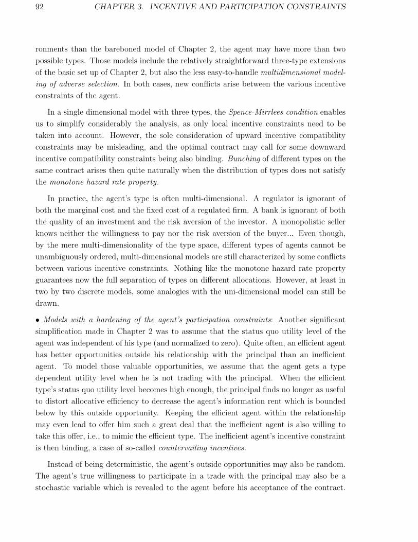
92 CHAPTER 3. INCENTIVE AND PARTICIPATION CONSTRAINTS
ronments than the bareboned model of Chapter 2, the agent may have more than two
possible types. Those models include the relatively straightforward three-type extensions
of the basic set up of Chapter 2, but also the less easy-to-handle multidimensional model-
ing of adverse selection. In both cases, new conflicts arise between the various incentive
constraints of the agent.
In a single dimensional model with three types, the Spence-Mirrlees condition enables
us to simplify considerably the analysis, as only local incentive constraints need to be
taken into account. However, the sole consideration of upward incentive compatibility
constraints may be misleading, and the optimal contract may call for some downward
incentive compatibility constraints being also binding. Bunching of different types on the
same contract arises then quite naturally when the distribution of types does not satisfy
the monotone hazard rate property.
In practice, the agent’s type is often multi-dimensional. A regulator is ignorant of
both the marginal cost and the fixed cost of a regulated firm. A bank is ignorant of both
the quality of an investment and the risk aversion of the investor. A monopolistic seller
knows neither the willingness to pay nor the risk aversion of the buyer... Even though,
by the mere multi-dimensionality of the type space, different types of agents cannot be
unambiguously ordered, multi-dimensional models are still characterized by some conflicts
between various incentive constraints. Nothing like the monotone hazard rate property
guarantees now the full separation of types on different allocations. However, at least in
two by two discrete models, some analogies with the uni-dimensional model can still be
drawn.
• Models with a hardening of the agent’s participation constraints: Another significant
simplification made in Chapter 2 was to assume that the status quo utility level of the
agent was independent of his type (and normalized to zero). Quite often, an efficient agent
has better opportunities outside his relationship with the principal than an inefficient
agent. To model those valuable opportunities, we assume that the agent gets a type
dependent utility level when he is not trading with the principal. When the efficient
type’s status quo utility level becomes high enough, the principal finds no longer as useful
to distort allocative efficiency to decrease the agent’s information rent which is bounded
below by this outside opportunity. Keeping the efficient agent within the relationship
may even lead to offer him such a great deal that the inefficient agent is also willing to
take this offer, i.e., to mimic the efficient type. The inefficient agent’s incentive constraint
is then binding, a case of so-called countervailing incentives.
Instead of being deterministic, the agent’s outside opportunities may also be random.
The agent’s true willingness to participate in a trade with the principal may also be a
stochastic variable which is revealed to the agent before his acceptance of the contract.

3.1. INTRODUCTION 93
This leads to random participation constraints and thus to a probabilistic participation of
some types. In a two-type model where only the inefficient type’s participation is random,
the contract must not only induce information revelation by the efficient type but must
also arbitrate between the benefit of trading more often with an inefficient one and the
cost of providing the latter type enough incentives to participate.
•Models with constraints on transfers: So far we have assumed that the monetary transfers
between the principal and the agent were unlimited. Several kinds of constraints can be
imposed on these transfers.
Under ex ante contracting and with a risk neutral agent, we showed in Section 2.12.1
that the first-best was implementable provided that the agent receives a negative pay-
off in the bad state of nature. However, agents are often financially constrained and
have limited liability. When such penalties are restricted by different kinds of limited
liability constraints, it becomes harder to induce information revelation. The conflict be-
tween incentive compatibility and ex ante participation constraints is no longer costless
to solve. second-best volumes of trade are then distorted away from the first-best values.
The direction of the distortion depends nevertheless of the nature of the limited liability
constraints.
In Section 2.15.1 we have already seen how informative signals on the agent’s type
enabled the principal to improve the terms of the rent extraction-efficiency trade-off.
Auditing is an endogenous way to obtain such signals. It is akin to a costly enlargement
of the principal’s tools available to screen the agent’s type. At some cost, the principal
may be able to verify with some probability the agent’s message on his type. In cases
where a lie is detected, the agent is punished and has to pay a penalty which, again, can
be limited in different ways by either the agent’s assets or his gains from trade with the
principal. Of course, this threat of an audit relaxes the incentive compatibility constraint.
But the trade-off between incentive compatibility and participation constraints is again
dependent on the particular constraints imposed on punishments.
Most of the book is concerned with principal-agent relationships where the conflict
between the principal and the agent is quite obvious and leads to binding participation
constraints. However, when the principal is a benevolent government willing to redis-
tribute income between heterogenous agents, the conflict comes from the interaction be-
tween the principal’s budget balance constraint and the agent’s incentive constraint. The
resolution of such problems does not use exactly the same methods as those we have used
so far. Indeed, for such models, one cannot determine sequentially, first, the distribution
of information rents which implement at a minimal cost a given output profile and, sec-
ond, the second-best outputs. Instead, the technical difficulties of such models come from
the simultaneous characterization of the second-best outputs and profiles of information

94 CHAPTER 3. INCENTIVE AND PARTICIPATION CONSTRAINTS
rents.
Section 3.2 presents the straightforward three-type extension of the standard model of
Chapter 2. We discuss there the Spence-Mirrlees and the monotone hazard rate property
which altogether ensure monotonicity of the optimal schedule of outputs and the absence
of any bunching of types. Section 3.3 deals with a bi-dimensional adverse selection model,
solving for the optimal outputs and comparing it with a standard uni-dimensional model.
Several economic applications are discussed. Section 3.4 offers a careful analysis of a
two-type model with reservation utilities, discussing all possible regimes of the solution.
We provide there various instances where this modeling has turned out to be useful to
understand various economic phenomena. Section 3.5 introduces random participation
constraints. In Section 3.6, we look at the impacts that different limited liability con-
straints, either on transfers or on rents, may have on the allocation of resources under ex
ante contracting. The first constraints increase the volume of trade as the second ones
reduce it. In Section 3.7, we analyze audit models and derive optimal audit policies under
various constraints for punishments. We draw there some analogy between audit models
and models where incentives for truthful revelation are based on the threat of terminat-
ing with some probability the relationship between the principal and the agent. Finally,
Section 3.8 analyzes the trade-off between efficiency and redistribution. It shows how to
optimize such efficiency-equity trade-offs.
3.2 More than Two Types
Suppose that θ may take three possible values, i.e., Θ = {θ, θ, θ} with θ− θ = θ− θ = ∆θ
for simplicity, and with respective probabilities ν, ν and ν such that ν + ν + ν = 1.
We denote by {(t, q), (t, q), (t, q)} a direct truthful revelation mechanism in this three-
type environment. Using similar notations, information rents write respectively as U =
t− θq, U = t− θq and U = t− θq. As a benchmark, note that the first-best outputs
are respectively given by S ′(q∗) = θ, S ′(q∗) = θ and S ′(q∗) = θ.
3.2.1 Incentive Feasible Contracts
For each of the three possible types, we have now the following incentive constraints: For
the most efficient type θ,
U ≥ U + ∆θq, (3.1)
U ≥ U + 2∆θq; (3.2)

3.2. MORE THAN TWO TYPES 95
for the intermediate type θ,
U ≥ U + ∆θq, (3.3)
U ≥ U −∆θq; (3.4)
for the least efficient type θ,
U ≥ U −∆θq, (3.5)
U ≥ U − 2∆θq. (3.6)
Les us show for example how (3.1) and (3.2) are obtained. We want that a θ-agent
does not announce θ. This requires:
U = t− θq ≥ t− θq = t− θq + (θ − θ)q (3.7)
or
U ≥ U + ∆θq. (3.8)
Also, we want that a θ-agent does not pretend to be θ. This requires:
U = t− θq ≥ t− θq = t− θq + (θ − θ)q (3.9)
or
U ≥ U + 2∆θq. (3.10)
Those six incentive constraints (3.1) to (3.6) can be classified into two categories: local
and global incentive constraints. Local incentive constraints involve adjacent types like
the upward incentive constraints (3.1) and (3.3) or the downward incentive constraints
(3.5) and (3.4). Global incentive constraints involve non-adjacent types like the upward
(3.2) or the downward (3.4) incentive constraint.
To simplify the analysis and find the relevant binding constraints, we proceed in two
steps. First, as in Chapter 2, intuition suggests that the most efficient types want to
lie upward and claim they are less efficient. Therefore, we can ignore momentarily the
downward constraints as we did in Chapter 2. We are left with the remaining upward
incentive constraints (3.1), (3.2) and (3.3).
Second, the incentive constraints (3.1) to (3.6) imply also some monotonicity condi-
tions on the schedule of outputs. Indeed, adding the incentive constraints for two adjacent
types yields q ≥ q (use (3.1) and (3.4)) and q ≥ q (use (3.3) and (3.5)). Finally, we get:
q ≥ q ≥ q. (3.11)

96 CHAPTER 3. INCENTIVE AND PARTICIPATION CONSTRAINTS
This monotonicity helps to further simplify the set of relevant incentive constraints by
getting rid of the global incentive constraint (3.2). Indeed, adding (3.1) and (3.3) yields:
U ≥ U + ∆θ(q + q). (3.12)
But using that q ≥ q, the second term right-hand side above is greater than 2∆θq.
Therefore, the global incentive constraint (3.2) is implied by the two local incentive con-
straints (3.1) and (3.3).
Finally, to obtain the optimal contract we will only consider the two upward local
incentive constraints with the monotonicity constraint on outputs (implying the global
upward constraint) and we will check ex post that the downward IC are also satisfied.
3.2.2 The Optimal Contract
This huge simplification in the set of incentive constraints being made, all relevant con-
straints for the principal reduce to the incentive constraints (3.1), (3.3), (3.11) and to the
least efficient type’s participation constraint:
U ≥ 0. (3.13)
The optimal contract solves thus the program (P ) below:
(P ) : max{(U,q);(U ,q);(U ,q)}
ν(S(q)− θq − U) + ν(S(q)− θq − U) + ν(S(q)− θq − U)
subject to (3.1), (3.3), (3.11) and (3.13).
It should be clear that constraints (3.1), (3.3), (3.13) are all binding at the optimum.
This leads to the following expressions of the information rents, U = ∆θ(q + q), U = ∆θq
and U = 0. Substituting into the objective function of problem (P ), we obtain that the
principal must solve program (P ′) below:
(P ′) : max{(q,q,q)}
ν(S(q)− θq −∆θ(q + q)
)+ ν(S(q)− θq −∆θq) + ν(S(q)− θq).
The next proposition summarizes the solution of the principal’s problem:
Proposition 3.1 : In a three type adverse selection model, the optimal contract entails:
• Constraints (3.1), (3.3) and (3.13) are all binding.

3.2. MORE THAN TWO TYPES 97
• When ν > νν, the monotonicity conditions (3.11) are strictly satisfied. Optimal
outputs are given by qSB = q∗, qSB < q∗ and qSB < q∗ with:
S ′(qSB) = θ +ν
ν∆θ, (3.14)
S ′(qSB) = θ +ν + ν
ν∆θ. (3.15)
• When ν < νν, some bunching emerges.We still have qSB = q∗ but now qSB = qSB =
qP < q∗ with:
S ′(qP ) = θ +2ν
ν + ν∆θ. (3.16)
When ν > νν, we have a straightforward extension of Proposition 2.1. The most
efficient type’s production level is not distorted. Since his information rent, namely U =
∆θ(q+ q), depends now on the production levels of all the types who are less efficient than
him, those production levels are distorted downward to reach the optimal rent extraction-
efficiency trade-off. The reason for this expression of the θ-agent’s rent is that all the
local upward incentive constraints are binding (and only those). The θ-agent has also an
information rent, U = ∆θq, as he can pretend to be a θ-agent. This justifies a second
downward distortion of q. Only the least efficient agent gets a zero rent U = 0. All these
features of the optimal contract are general and hold for any number of types.
If the profile of production levels obtained satisfies the monotonicity conditions (3.11),
all the other incentive constraints also hold strictly. If not, some bunching emerges as
described in the second part of Proposition 3.1. We have already seen in Chapter 2 how
bunching may arise at the optimal contract when the principal’s and the agent’s objectives
are strongly conflicting (see Section 2.11.2). Here, the origin of bunching is that the
principal would like to implement an increasing second-best schedule of output over some
range of types (namely q > q), but this monotonicity conflicts with the monotonicity
condition imposed by incentive compatibility. This can be viewed, again, as an instance
of non-responsiveness.2 Such phenomenon appears only when there are more than two
types or with a continuum. Remember, indeed, that it never holds in the standard two
type model of Section 2.4. To avoid it, modelers have often chosen to impose a sufficient
condition on the distribution of types, the “monotonicity of the hazard rate”.
Definition 3.1 : A distribution of types satisfies the monotone hazard rate property if
and only if:
Pr(θ < θ)
Pr(θ = θ)=
ν
ν<
Pr(θ < θ)
Pr(θ = θ)=
ν + ν
ν. (3.17)
2See Appendix 3.1 for an analysis of bunching in the case of a continuum of types.

98 CHAPTER 3. INCENTIVE AND PARTICIPATION CONSTRAINTS
This sufficient condition ensures that the incentive distortions on the right-hand sides
of (3.14) and (3.15) are increasing with the agent’s type. The virtual costs of the different
types, namely θ, θ + νν∆θ and θ + ν+ν
ν∆θ, are thus ranked exactly as the true physical
costs. Asymmetric information does not perturb the ranking of types.
Remark: With n types, i.e., Θ = {θ1, . . . , θn} and a distribution of types such that
Pr(θi) = νi > 0 for all i, the monotonicity of the hazard rate property says that Pr(θ<θi)Pr(θ=θi)
=∑i−1k=1 νk
νiis increasing in i.
3.2.3 The Spence-Mirrlees Condition with more than Two Types
When the local incentive constraints imply the global ones, it is sufficient to check that
the agent does not want to lie locally to be sure that he does not want to lie globally. The
incentive problem is then well behaved since there is a huge simplification in the number
of relevant constraints. This is precisely this simplification which yields the clear analysis
in the last section. This huge simplification holds for any number of types or even for a
continuum if the agent’s utility function satisfies the so-called Spence-Mirrlees condition,
i.e., if the agent’s objective function U(q, t, θ), which is defined over allocations (q, t) in
A and types θ in Θ, is such that the marginal rates of substitution between output and
money can be ranked in a monotonic way. The following property must thus be satisfied:
∂
∂θ
(Uq
Ut
)> 0
(or < 0)for any (t, q, θ) in A×Θ. (3.18)
Economically, this property means that the indifference curves move always in the
same direction as θ changes. In Figure 3.1 below, we have drawn the case where the
marginal rates of substitution Uq
Ut, which is also the slope of the agent’s indifference curve,
are increasing with the agent’s type. At point A where the indifference curves of a θ-and
a θ-type cross each other, the indifference curve of the θ-type has a greater slope.

3.2. MORE THAN TWO TYPES 99
-
6
t
q
θ
θ
θ θθ
θ
•A
Figure 3.1: The Spence-Mirrlees Property.
Of course, the particular objective function used in Chapter 2 and in Section 3.2.1,
namely U = t− θq, satisfies the Spence-Mirrlees condition since ∂∂θ
(Uq
Ut
)= −1.
-
6
t
q
½½
½½
½½
½½
½½
½½
½½
½½
½½
½½
½½
·······················
»»»»»»»»»»»»»»»»»»»»»»»»»
•
•
•S
So
q q q
t
t
t
t = θqt = θq + ∆θq
t = θq + ∆θ(q + q)
A
B
C
Figure 3.2: Indifference Curves with Three Types and U = t− θq.
Figure 3.2 illustrates why the Spence-Mirrlees condition ensures that, when upward

100 CHAPTER 3. INCENTIVE AND PARTICIPATION CONSTRAINTS
local incentive constraints are binding, global ones and downward ones are strictly satis-
fied. As it can be easily seen from the figure, the efficient type is just indifferent between
telling the truth and lying upward to θ, i.e., he is indifferent between contracts A and B.
However, lying upward up to θ would reduce significantly his utility level, since contract C
is on an indifference curve with a lower level of utility than what a θ-type get by choosing
A. Hence, the θ-type’s global incentive constraint is satisfied. Similarly, consider an agent
with type θ. This agent is indifferent between telling the truth and lying upward up to θ.
He is indifferent between choosing B and C. However, by lying downward, type θ could
get contract A which yields him a strictly lower utility level. The downward incentive
constraint is strictly satisfied.
The Spence-Mirrlees conditions make the incentive problem well-behaved in the sense
that only local constraints need to be considered. It is similar to a concavity condition
in usual maximization problems. As for a concavity condition, the optimization of the
agent’s problem is obtained by looking at the benefits of “local” changes away from his
truthful report strategy, as “global” changes are certainly dominated. The analysis of
such situations is then very similar to that developed in Chapter 2.
When the Spence-Mirrlees condition is satisfied, the above analysis can also be easily
extended3 to the case of a continuum of types [θ, θ] already considered in Appendix 2.1. If
it is not satisfied, the analysis of the continuum case becomes quickly untractable, and the
study of the finite type case requires to consider all combinations of binding constraints
and calls very quickly for numerical methods.
Spence (1973) introduced the single-crossing assumption in his theory of sig-
naling. Similarly, Mirrlees (1971) used also such an assumption in his theory of opti-
mal income tax. It was called the constant sign assumption in Guesnerie and Laffont
(1984). Araujo and Moreira (2000) provides an analysis of optimal contracts when the
Spence-Mirrlees assumption may not be satisfied and types are distributed continuously.
Matthews and Moore (1987) provides an extensive study of the set of incentive constraints.
3.3 Multi-dimensional Asymmetric Information
3.3.1 A Discrete Model
Another important limitation of our analysis of adverse selection in Chapter 2 is that
the adverse selection parameter θ was modeled as a uni-dimensional parameter. In many
3See Appendix 3.2.

3.3. MULTI-DIMENSIONAL ASYMMETRIC INFORMATION 101
instances, the agent knows several pieces of information which are payoff relevant and
affect the optimal trade. For instance, a tax authority would like to know both the
elasticity of an agent’s labor supply and his productivity before fixing his tax liability.
Similarly, an insurance company would like to know both the probability of accident of an
agent and his degree of risk aversion before fixing the risk premium that this agent should
pay. The producer of a good knows not only his marginal cost of producing this good,
but also the associated fixed cost. In all these situations, the uni-dimensional paradigm
must be given up to assess the true consequences of asymmetric information on the rent
extraction-efficiency trade-off.
We extend now the analysis of Chapter 2 to the case of multi-dimensional asymmetric
information. The simplest way to do so is to have the agent accomplish two activities
for the principal. Let us thus assume that the agent produces two goods in respective
quantities q1 and q2 with a utility function U = t − (θ1q1 + θ2q2) with θi in {θ, θ}, for
i = 1, 2. We also assume that there is no externality between the two tasks for the
principal so that the surpluses associated with both tasks just add up in the latter’s
objective function which becomes V = S(q1) + S(q2)− t.
The probability distribution of the adverse selection vector θ = (θ1, θ2) (which is again
common knowledge) is now defined by ν = Pr(θ1 = θ, θ2 = θ), ν2
= Pr(θ1 = θ, θ2 = θ) =
Pr(θ1 = θ, θ2 = θ), ν = Pr(θ1 = θ, θ2 = θ) with a positive correlation among types being
defined as ρ = νν − ν2
4> 0.
The components of the direct revelation mechanism are denoted as (t11, q11, q11) if
(θ1 = θ, θ2 = θ), (t12, q12, q21) if (θ1 = θ, θ2 = θ), (t12, q21, q12) if (θ1 = θ, θ2 = θ),
(t22, q22, q22) if (θ1 = θ, θ2 = θ), where we impose (without loss of generality) a symmetry
restriction or transfers. Similar notations are used for the information rents Uij. Because
of the symmetry of the model, there are only three relevant levels of information rents
U = U11, U = U12 = U21 and U = U22. Similarly, we denote outputs by q11 = q, q12 = q2,
q21 = q1 and q22 = q, and transfers by t11 = t, t21 = t12 = t, t22 = t. These notations,
even though they look quite cumbersome, unify the present multi-dimensional modeling
with that of Section 3.2.1 above.
Again, following the logic of the uni-dimensional model we may guess that only the
upward incentive constraints matter. The three following incentive constraints become
then relevant:
U = t− 2θq ≥ t− θ(q1 + q2) = U + ∆θq1, (3.19)
U ≥ t− 2θq = U + 2∆θq, (3.20)
U = t− (θ + θ)q ≥ t− (θ + θ)q = U + ∆θq. (3.21)
We can expect also the participation constraint of an agent who is inefficient on both

102 CHAPTER 3. INCENTIVE AND PARTICIPATION CONSTRAINTS
dimensions (θ1 = θ and θ2 = θ) to be binding, i.e.:
U = 0. (3.22)
Moreover, we let the reader check that adding incentive constraints for types taken
two by two yields the following monotonicity conditions on outputs:
q ≥ max(q1, q), (3.23)
and
q2 ≥ max(q1, q). (3.24)
3.3.2 The Optimal Contract
We can expect (3.21) to be binding at the optimum. Then (3.19) and (3.20) can be
summarized as:
U ≥ ∆θ max(2q, q + q1), (3.25)
which should also be binding at the optimum.
After substitution of the information rents as functions of outputs, the principal’s
optimization program becomes:
(P ′) : max{(q,q,q)}
ν(2S(q)− 2θq −∆θ max(2q, q1 + q))
+ν(S(q1) + S(q2)− θq2 − θq1 −∆θq) + ν(2S(q)− 2θq).
We must distinguish two cases depending on the level of correlation ρ between both
dimensions of adverse selection.
Case 1: Weak Correlation
Let us first assume that the solution is such that q ≤ q1. In this case, max(2q, q1+ q) =
q1 + q and optimizing (P ′) yields the following second-best outputs:
S ′(qSB) = S ′(qSB2 ) = θ, (3.26)
S ′(qSB1 ) = θ +
ν
ν∆θ, (3.27)
S ′(qSB) = θ +ν + ν
ν∆θ, (3.28)

3.3. MULTI-DIMENSIONAL ASYMMETRIC INFORMATION 103
This latter schedule of outputs is really the solution when the monotonicity condition
qSB ≤ qSB1 holds, i.e., when:
ν
ν≤ ν + ν
ν, (3.29)
or to put differently when ρ ≤ ν(ν+ 34ν). This condition obviously holds in the case where
θ1 and θ2 are independently drawn since then the correlation is zero, i.e., ρ = 0. We let
the reader check that all neglected incentive and participation constraints are satisfied
when (3.29) is satisfied.
The binding constraints in the case of weak correlation are only the local ones. In
Figure 3.3 below, an arrow from a point in the type space, say A, to another one, say B,
means that A is “attracted” by B, i.e., the corresponding incentive constraint is binding
at the optimum.
-
6
•θ
θ2
θ
θ
θ1
θ
>
>
∧∧
Figure 3.3: Binding Incentive Constraints with a Weak Correlation.
Case 2: Strong Correlation
If we had perfect correlation ν = 0, the binding constraint would obviously be from (θ, θ)
to (θ, θ) (see Figure 3.4).
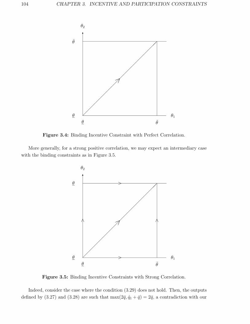
104 CHAPTER 3. INCENTIVE AND PARTICIPATION CONSTRAINTS
6
θ
θ
θ θ
θ2
θ1¡
¡¡
¡¡
¡¡
¡¡
¡¡
¡¡
¡¡
¡¡
¡¡
!!¯
Figure 3.4: Binding Incentive Constraint with Perfect Correlation.
More generally, for a strong positive correlation, we may expect an intermediary case
with the binding constraints as in Figure 3.5.
6
θ
θ
θ θ
>
>
∧∧
θ2
θ1¡
¡¡
¡¡
¡¡
¡¡
¡¡
¡¡
¡¡
¡¡
¡¡
!!¯
Figure 3.5: Binding Incentive Constraints with Strong Correlation.
Indeed, consider the case where the condition (3.29) does not hold. Then, the outputs
defined by (3.27) and (3.28) are such that max(2q, q1 + q) = 2q, a contradiction with our

3.3. MULTI-DIMENSIONAL ASYMMETRIC INFORMATION 105
starting assumption q ≤ q1. Let us thus assume that we have instead q > q1. In this case
optimizing (P ′) leads to the substitution of (3.27) and (3.28) by respectively:
S ′(q1) = θ, (3.30)
and
S ′(q) = θ +2ν + ν
ν∆θ. (3.31)
But, we immediately observe that q < q1; again this is a contradiction with our starting
assumption q > q1.
When (3.29) does not hold, we have thus necessarily q1 = q = qP and bunching
arises at the optimal contract. To understand the origin of this bunching, first note that,
because of a strong correlation, the probability that mixed states (θ, θ) occur is small.
Hence, because he fears mostly the global deviation where a (θ, θ)-type claims he is (θ, θ),
the principal would like to implement a high output q1 without much distortion. But by
doing so, the allocation of a (θ, θ)-agent becomes very attractive to the most efficient type
on both dimensions (θ, θ). This pushes now the principal to distort output q1 downward.
Torned between those two opposite incentives, the principal chooses to bunch the outputs
q1 and q.
Optimizing (P ′) with this added constraint still yields (3.26) but also
S ′(qP ) = θ +ν + ν
ν + ν∆θ. (3.32)
We can note the strong analogy between the multi-dimensional case and what we have
seen for a uni-dimensional parameter both in Chapter 2 and in Section 3.2 above. First,
note that, for a weak correlation between types, the asymmetric information distortions
on the right-hand sides of (3.27) and (3.28) are the same as those on the right-hand sides
of (3.14) and (3.15). In this case, the 4-type bi-dimensional model almost boils down to a
3-type one dimensional model. Everything happens as if there were only three fictitious
types which could be denoted by θ, θ and θ with respective probabilities ν, ν and ν and
a single dimension of output. Second, for a strong correlation, the 4-type bi-dimensional
model is almost like a 2-type uni-dimensional model with distortions similar to those of
Proposition 2.1. Everything happens now as if there were only two fictitious types θ and
θ with respective probabilities ν + ν2
and ν2
+ ν and, again, a single dimension of output.
These two results yield an important insight. In a multi-dimensional world, it is easy to
construct examples where, at the optimum, everything happens as if the principal was
using a message space with the agent which has a much lower dimensionality than the
type space itself. The detour of modeling a more complex environment also brings some
“simplicity” into the optimal contract.

106 CHAPTER 3. INCENTIVE AND PARTICIPATION CONSTRAINTS
We summarize our findings in the next proposition:
Proposition 3.2 : In a symmetric bi-dimensional adverse selection setting, the optimal
contract with a weak correlation of types keeps many features of the uni-dimensional case.
With a strong correlation, the optimal contract may instead entail some bunching.
Finally, note that more complex situations arise when the correlation is negative,
asymmetric distributions are postulated, or when the dimensionality of actions is not the
same as the dimensionality of the asymmetry of information.
We now describe a number of settings where modeling adverse selection with multi-
dimensional types has proved to be useful.
Example 1: Unknown Fixed Cost
Let us suppose that the agent has a cost function C(θ, q) = θ1q + θ2 where both the
marginal cost θ1 and the fixed cost θ2 are now unknown. As shown in Baron and Myerson
(1982) and Rochet (1984), stochastic mechanisms where the decision to produce or not
is used as a screening device are useful in this context. To see why, let us introduce x in
{0, 1} as a dummy variable which is equal to 1 when a positive production is requested
and 0 otherwise. As a function of the contracting variable q and x, the agent’s utility
function writes now as U = t − (θ1qx + θ2x) and this expression almost takes the same
form as what we have analyzed above. It is easy to show that the shut-down of some
types is also a valuable screening device to learn the value of the fixed cost θ2.
Example 2: Unknown Cost and Demand
Let us assume that the agent is a retailer who serves a market with a linear inverse
demand P (q) = a− θ1 − q, where θ1 is an intercept parameter which is the first piece of
private information of the agent. This agent has also a cost function C(q) = θ2q where the
marginal cost θ2 is the second piece of private information of the agent. The latter’s utility
function writes finally as U = t+(a− θ1− q)q− θ2q, where t is the transfer received from
the principal, here a manufacturer. To simplify, we also assume that the manufacturer
incurs no production cost for the intermediate good he provides to the agent. Introducing
a new variable t = t+aq−q2, the agent’s utility function rewrites as U = t−(θ1q1 +θ2q2).
On the other hand, the principal’s objective becomes V = aq − q2 − t.
We can then apply the previous analysis to compute the characteristics of the optimal
contract. Interestingly, a strong correlation between cost and demand parameters calls for
a relatively inflexible contract with an “almost” fixed quantity being sold on the market.
This may explain the relative simplicity of some vertical restraint arrangements between
manufacturers and retailers.

3.3. MULTI-DIMENSIONAL ASYMMETRIC INFORMATION 107
3.3.3 Continuum of Types
In Chapter 2 and in its Appendix 2.1 we have argued that the discrete model and the
model with a continuum of types were economically quite similar. Things are a little
bit different with multi-dimensional asymmetric information. The dimensionality of the
type space plays indeed a crucial role. To see this point, recall that, in a one dimensional
case, the least efficient type’s participation constraint is the only binding participation
constraint (at least as long as shut-down is not optimal). Now imagine that the same
holds with a continuum of bi-dimensional types, i.e., only the “least” efficient type on
both dimensions θ1 and θ2, i.e., (θ, θ), is put at its reservation utility. Let us imagine that
the principal slightly decreases uniformly by ε the whole transfer schedule he offers to the
agent. Of course, a whole subset of types around (θ, θ) prefers to stop producing. The
efficiency loss for the principal is roughly of order ε2. However, by reducing uniformly
the whole transfer schedule, the principal reduces all information rents of the remaining
types by ε, hence he makes a gain worth ε(1 − ε2) ≈ ε. Therefore, the shut-down of a
subset of types with non-zero measure is always optimal.4
Armstrong and Rochet (1999) provided a complete analysis of the two type
model. The case of a continuum of types has first been analyzed by McAfee and McMil-
lan (1988) who attempted to generalize the Spence-Mirrlees assumption to a multi-
dimensional case and Laffont, Maskin and Rochet (1987) who solved explicitly an example.
The result that shut-down of types is always optimal is due to Armstrong (1996) who also
offers some closed-form solutions when the set of types includes the origin. These tech-
niques are difficult and outside the scope of the present volume. See also Wilson (1993)
on this point. Rochet and Chone (1998)’s analysis is the most general. They showed that
bunching of types is always found in these multi-dimensional models and they provide
also the so-called “ironing and sweeping” techniques designed at analyzing this bunching
issue. Finally, Armstrong (1999) pushed the idea that multi-dimensional adverse selec-
tion problems may introduce a significant simplification in the optimal contract between
a seller and a buyer privately informed on his type. Instead of explicitly computing this
contract, he provides a lower bound on what can be achieved with simple two part tariffs
and, using the Law of Large Numbers, shows that those contracts can approximate the
first-best when the number of products sold to this buyer is large enough.
4Note that this dimensionality argument fails for a discrete n2−type model since the loss of efficiencyand the saving on information rent have the same dimensionality.

108 CHAPTER 3. INCENTIVE AND PARTICIPATION CONSTRAINTS
3.4 State Dependent Status Quo Utility Level and
Countervailing Incentives
The models of Sections 3.2 and 3.3 have already illustrated the difficulties that the modeler
faces when there may be no obvious order between the various incentive constraints. The
same kind of difficulties arise when the agent’s participation constraint is type dependent.
Indeed, those participation constraints may perturb the natural ordering of the incentive
and participation constraints studied in Chapter 2. To analyze those issues, we now
come back to our two type model. In Chapter 2 we made a simplifying and debatable
assumption by postulating that the outside opportunities of the two types of agents were
identical (and without loss of generality normalized to zero). Then, we know that the
binding incentive constraint is always the efficient type’s one. However, in many cases
there is a correlation (in general a positive one) between the agent’s productivity in a
given principal-agent relationship and his outside opportunity. We assume now that the
efficient agent’s outside utility level is U0 > 0 and we still normalize to zero the inefficient
agent’s one.
The efficient and inefficient type participation constraints write now respectively as:
U ≥ U0 (3.33)
U ≥ 0. (3.34)
3.4.1 The Optimal Contract
The principal’s problem writes thus as optimizing (2.19) subject to the relevant downward
incentive compatibility constraint (2.22) to (2.23) and the new type-dependent partici-
pation constraints (3.33) and (3.34). The solution to this problem exhibits five different
regimes depending on the value of U0.
Case 1- Irrelevance of Outside Opportunity: U0 < ∆θqSB
Then, the optimal second-best solution (2.22), (2.24), (2.26) obtained in Section 2.7 re-
mains valid since the neglected participation constraint (3.33) is satisfied by the solution
discussed in Proposition 2.1. When the outside option does not provide too much rent to
the efficient agent, it does not affect the second-best contract.
Case 2- Binding Outside Opportunity and Incentive Constraints: ∆θq∗ > U0 >
∆θqSB
The former solution is now no longer valid. To induce his participation more rent must be
given up to the efficient type than the information rent obtained in the optimal second-best

3.4. STATE DEPENDENT 109
contract corresponding to U0 = 0. Then, one can afford less distorsion in the inefficient
type’s production level and choose q such that U0 = ∆θq. As long as U0 belongs to
[∆θqSB, ∆θq∗], the incentive constraint of the efficient type and both participation con-
straints are simultaneously binding. (See for example the pair of contracts (A0, B0) in
Figure 3.6).
-
6
t
q³³³³³³³³³³³³³³³³³³³³³³³³³³³³
¡¡
¡¡
¡¡
¡¡
¡¡
¡¡
¡¡
¡¡
¡¡
¡¡
¡¡
¡
!!!!!!!!!!!!!!!!!!!!!!!!!!!!!
!!!!!!!!!!!!!!!!!!!!!!!!!!!!!
!!!!!!!!!!!!!!!!!!!!!!!!!!!!!!
••
•
q∗qqSB
•••
•
C
B∗
B0
BSB
A0
ASB
A∗
∆θqSBU0
Figure 3.6: Type-Dependent Participation Constraint: Case 2.
Case 3- Both Outside Opportunities Constraints Are Binding: ∆θq∗ > U0 >
∆θq∗
Still raising U0, the principal finds now no longer optimal to use the inefficient type’s
output to raise the efficient agent’s information rent and induce his participation. This
output being already efficient, the only remaining tool available to the principal to raise
the efficient agent’s rent is the transfer t and we have now t = θq∗ + U0. This solution is
obviously valid as long as the inefficient agent’s incentive constraint is not binding, i.e.,
as long as 0 = U > U0 − ∆θq∗. (See the pair of contracts (A0, B0) in Figure 3.7. This
case remains valid as long as A0 is below D). In that region, both production levels are
the efficient ones.
Case 4- The Inefficient Agent’s Incentive Constraint is Binding: U0 ≥ ∆θq∗
When U0 still increases (A0 would be above D), the inefficient type is now attracted by
the allocation given to the efficient type but both constraints (3.33) and (3.34) remain

110 CHAPTER 3. INCENTIVE AND PARTICIPATION CONSTRAINTS
binding. As a result, the efficient agent’s output is upward distorted to reach a value q
defined by U0 = ∆θq
-
6
t
q¡¡
¡¡
¡¡
¡¡
¡¡
¡¡
¡¡
¡¡
¡¡
¡¡
¡¡
¡¡¡
³³³³³³³³³³³³³³³³³³³³³³³³³³³³³
³³³³³³³³³³³³³³³³³³³³³³³³³³³³³
³³³³³³³³³³³³³³³³³³³³³³³³³³³
³³³³³³³³³³³³³³³³³³³³³³³³³³³³³
U0
•
•
•
•
•
•
q∗ q∗
A0
D
ACI
BCI
BSB = B0
•
•C
ASB
Figure 3.7: Type-Dependent Participation Constraint: Case 4.
Case 5- The Efficient Type’s Participation Constraint and the Inefficient Type’s
Incentive Constraint Are Both Binding: U0 > ∆θqCI
Let us maximize (2.19) under the constraints (3.33) and (2.23). Assuming that those two
constraints are binding, we obtain U = U0 and U = U0−∆θq. Inserting, those expressions
into the principal’s objective function, we get a reduced form program given by:
(P ) : max{(q,q)}
ν(S(q)− θq) + (1− ν)(S(q)− θq) + (1− ν)∆θq − U0.
Optimizing with respect to outputs yields no distortion for the inefficient type who
produces qCI = q∗ and now an upward distortion for the efficient type qCI > q∗ such that:
S ′(qCI) = θ − 1− ν
ν∆θ, (3.35)
where the superscript CI means countervailing incentives. As U0 becomes greater than
∆θqCI , a rent UCI = U0 −∆θqCI is now given up to the inefficient type (see the pair of
contracts (ACI , BCI) in Figure 3.8).

3.4. STATE DEPENDENT 111
-
t
q³³³³³³³³³³³³³³³³³³³³³³³³³³³
¡¡
¡¡
¡¡
¡¡
¡¡
¡¡
¡¡
¡¡
¡¡
¡¡
¡¡
¡¡¡
¡¡
¡¡
¡¡
¡¡
¡¡
¡¡
¡¡
¡¡
¡¡
¡¡
¡¡
¡
•
•6
?
U
BCI
BSB = B0
•A
•D
•ACI
q∗ q∗ qSBCI
6
Figure 3.8: Type-Dependent Participation Constraint: Case 5.
-
6
´´
´´
´´
´´
´´
´´
qSB
q∗
q∗
qCI
∆θqSB ∆θq∗ ∆θq∗ ∆θqSBU0
(ICP
) IC
PP
(
PP
) P
PIC
(
PIC
)
qBBN
qBBN
Figure 3.9 Type-Dependent Participation Constraint: Output Distortions.
112 CHAPTER 3. INCENTIVE AND PARTICIPATION CONSTRAINTS
Figure 3.9 summarizes the profiles of production levels as functions of the efficient
type’s outside opportunity utility level U0. For U0 higher than ∆θq∗, we are in the case
of countervailing incentives. To attract the efficient type who has such profitable outside
opportunities it is necessary to offer him a very high transfer. But then this contract
becomes attractive for the inefficient type who now captures a strictly positive rent. To
decrease this costly rent the production level of the efficient type is now distorted. But it
is distorted upwards rather than downwards because the inefficient type’s rent, U0−∆θq,
is decreasing with q.
Type dependent utilities with interesting economic implications have successively
appeared in Moore (1985) for a model of labor contracts, Lewis and Sappington (1989) for
an extension of the Baron and Myerson (1982) regulation model with fixed costs, Laffont
and Tirole (1990) for the regulation of bypass, Feenstra and Lewis (1991) and Brainard
and Martimort (1996) for models of international trade and, finally, Jeon and Laffont
(1999) for a model of downsizing the public sector. Jullien (2000) provides a general
theory of type-dependent reservation utility with a continuum of types.
3.4.2 Countervailing Incentives: Examples
State Dependent Fixed Costs
Lewis and Sappington (1989) (who have coined the expression countervailing incentives)
reconsidered the Baron-Myerson model with a firm having a fixed cost negatively corre-
lated with its marginal cost. The firm’s cost function is C(θ, q) = θq + F (θ), where θ
belongs to {θ, θ} with respective probabilities ν and 1− ν. The fixed costs are such that
F (θ) > F (θ), i.e., high marginal costs are associated with low fixed costs and vice versa.
In this model, incentive constraints are still unchanged and expressed as (2.20) and
(2.21). The participation constraints become instead
U ≥ F (θ) = F (θ) + (F (θ)− F (θ)) (3.36)
and
U ≥ F (θ). (3.37)
It should be clear, that, up to a constant term F (θ), the model is identical to that of
Section 3.4.1. F (θ)−F (θ) > 0 plays exactly the role of U0 and may lead to countervailing
incentives if it is large enough.

3.4. STATE DEPENDENT 113
Lewis and Sappington (1989) studied a model with a continuum of types and
emphasized the bunching region they obtain in the transition from upward to downward
binding incentive constraints. Maggi and Rodriguez-Clare (1995a) showed that bunching
is due to the concavity that Lewis and Sappington assume for the F (·) function. If F (·)is convex, countervailing incentives are compatible with fully separating contracts. To
investigate these issues in a discrete example requires a three type model.
With more than two types, let us say three as in Section 3.2, or with a continuum,
it may be that a given type θ attracts both types θ which are immediately above and
below it. The fact that θ attracts more efficient types calls for distorting downwards
output for the types close but below θ. The fact that θ attracts also less efficient types
calls for distorting upwards output for the types close to θ from above. These two distor-
tions conflict with the monotonicity requirement that output should remain decreasing
everywhere. Countervailing incentives create thus some pooling for intermediate types.
In a related context, the optimal contract has been interpreted by Lewis and Sappington
(1991) as an inflexible rule coming from the existence of countervailing incentives.
Bypass
Laffont and Tirole (1990) considered consumers of a network technology such as electricity.
They are of two possible types θ and θ having utility function U = θv(q) − t. Those
consumers can either consume the good produced by the network technology which offers
a menu of contracts,{(t, q), (t, q)
}, or they can use an alternative bypass technology
which has a fixed cost σ and a marginal cost d. By choosing this latter option, consumers
obtain the utility levels S = maxq{θv(q)− σ − dq} and S = maxq{θv(q)− σ − dq}. The
consumers’ participation constraints become then:
U = θv(q)− t ≥ S (3.38)
U = θv(q)− t ≥ S = S + S − S. (3.39)
Up to a change in the definition of the “efficient” and the “inefficient” type, S−S plays
here the role of U0 in Section 3.4.1 and can again give rise to countervailing incentives.
When the network industry is very efficient, a regulated or profit maximizing network
attracts all consumers with a discriminating menu of contracts. As its efficiency deterio-
rates, it must distort the pricing scheme to maintain the high valuation consumers in the
network and the good deal made to these consumers may attract low valuation consumers
and create countervailing incentives. Finally, as efficiency deteriorates further, the profit
maximizing network lets the high valuation consumers leave the network.

114 CHAPTER 3. INCENTIVE AND PARTICIPATION CONSTRAINTS
Downsizing the Public Sector
An inefficient public sector exhibits sometimes a considerable labor redundancy. Hence,
downsizing constitutes a natural step for every public sector reform. However, downsizing
is subject to adverse selection. To model this issue, Jeon and Laffont (1999) assumed that
a worker of the public firm has a private cost θ in {θ, θ} when working in that firm. Let
Up(θ) be the rent obtained by a θ-worker in the public firm and Um(θ) be the rent he
would obtain in the private sector with the normalization Um(θ) = 0.
A (voluntary) downsizing mechanism for a continuum [0, 1] of workers is a pair of
transfers and probabilities5 of being maintained in the firm, {(t, q), (t, p)}, which must
satisfy the participation constraints
U = t− pθ + (1− p)Um(θ) ≥ Up(θ) (3.40)
U = t− pθ ≥ Up(θ), (3.41)
and the incentive constraints
U = t− pθ + (1− p)Um(θ) ≥ t− pθ + (1− p)Um(θ) = U + p∆θ + (1− p)Um(θ) (3.42)
U = t− pθ ≥ t− pθ = U − q∆θ. (3.43)
If we define the worker’s full costs θf as the sum of the production cost and his rent in
the private sector, θf = θ + Um(θ), these equations can be rewritten as:
U = t− pθf ≥ Up(θ)− Um(θ) (3.44)
U = t− pθf ≥ Up(θ) (3.45)
U = t− pθf ≥ t− pθf = U + p∆θ (3.46)
U = t− pθf ≥ t− pθf = U − p∆θ. (3.47)
We can reduce the problem to the one treated in Section 3.4, if we rewrite the partic-
ipation constraints in the following manner:
U ≥ Up(θ) (3.48)
U ≥ Up(θ) + Up(θ)− Up(θ)− Um(θ). (3.49)
Defining U0 = Up(θ)− Up(θ)− Um(θ) we could proceed as in Section 3.4.
If θf > θf , i.e., ∆θ > Um(θ), the worker with production cost θ remains the low full
cost worker. If furthermore, Up(θ) − Up(θ) = ∆θ, i.e., the discrimination in the public
5These probabilities can also be interpreted as part time work in the public firm.

3.4. STATE DEPENDENT 115
firm fits the productivity difference, then U0 = ∆θf and we have necessarily countervailing
incentives. The rent of the high full cost is then Up(θ)−Um(θ)−p∆θf and to decrease this
information rent p is increased. This means that downsizing decreases under asymmetric
information. This situation is illustrated in Figure 3.10.
-
6
t
p
0
´´
´´
´´
´´
´´
´´
´´
´´
´´
´´
´´
´´
´´
´
(((((((((((((((((((((((((((((((((
•B •
B′′ •
•A
•A′′
•A′
Up(θ)
Up(θ) + U0
p∗ pSB 1
t = Up(θ) + θfp
t = Up(θ) + U0 + θfp
Figure 3.10: Downsizing the Public Sector.
Consider a case where downsizing is large and the complete information downsizing
entails excluding all the inefficient workers (contract A) and a proportion p∗ of efficient
ones (contract B). Under incomplete information this requires giving up a rent AA′ to the
inefficient type and creates countervailing incentives. To decrease this rent p is increased
to pSB (contracts (A′′, B′′)).
If θf < θf the high full cost is then the worker with low production cost. But we have
again countervailing incentives and the rent of the high full cost is p∆θf + Up(θ). Now
∆θf < 0 and p is decreased. Downsizing decreases also under incomplete information,
but now the workers with low production costs are excluded first.
International Trade and Protection
Private industries subject to international competition often call for some protection from
their national government to avoid delocalisation. The goal of public intervention in such

116 CHAPTER 3. INCENTIVE AND PARTICIPATION CONSTRAINTS
a context is first to provide domestic firms with at least their profits in the international
arena and, second, as in domestic regulation, to correct any market power.
To model such issues, let us consider a variation of the Baron-Myerson model discussed
in Section 2.17.1. The domestic regulator maximizes S(q + qf ) − pwqf − θq − (1 − α)U
where qf is foreign production imported at the world price pw. The domestic firm’s utility
function is U = t − θC(q) with C(q) = q2
2. Decreasing returns are here necessary to
have the national consumption being split in a non trivial way between national and
foreign productions. Again, the efficiency parameter θ can take values in Θ = {θ, θ} with
respective probabilities ν and 1− ν.
It is clear that the first-best outcome is such that the domestic firm produces at the
world price, the residual domestic demand being imported at this price. This leads to
pw = θq∗ and pw = θq∗.
Under asymmetric information and if regulation applies to a national public enterprise
having no outside option, the second best policy becomes qSB = q∗ and qSB given by:
pw =
(θ +
ν
1− ν(1− α)∆θ
)qSB. (3.50)
Consider now a private enterprise which could take all its assets away from the national
country and behave competitively in the world market. Participation constraints become
for type θ and θ respectively:
U ≥ U0 = maxq
pwq − θC(q) =p2
w
2θ, (3.51)
and
U ≥ U0 = maxq
pwq − θC(q) =p2
w
2θ. (3.52)
In this model, we can redefine U0 as U0 = U0 − U0 = p2w∆θ
2θθ. The information rents
corresponding to the first-best outputs q∗ and q∗ are now∆θq∗2
2and ∆θq∗2
2. Hence
∆θq∗2
2>
U0 > ∆θq∗22
and we are (up to a change in the cost function) in Case 3 above, leading to
no countervailing incentives.
Insurance Contracts
Standard microeconomics analysis shows that, under complete information, all agents
subject to some risk should receive complete insurance against this risk. This conclusion
fails under asymmetric information. Let us consider a risk averse agent with utility

3.4. STATE DEPENDENT 117
function u(·) which is increasing and concave (u′(·) > 0, u′′(·) < 0 with u(0) = 0). The
agent’s initial wealth is w, but with probability θ the agent suffers from a damage which
has value d. The agent is a low risk θ < 1 (resp. high risk θ < θ < 1) with probability
1 − ν (resp. ν). The agent knows his probability of accident which remains unknown
from an insurance company. The agent’s wealth level is common knowledge. The agent’s
expected utility writes thus as U = θu(w − d + ta) + (1 − θ)u(w − tn) where ta is the
agent’s reimbursement in case of a damage and tn is what he pays to the insurance
company when there is no accident. Much of the technical difficulties encountered with
this model will come from the nonlinearity of the agent’s utility function with respect
to transfers. Note nevertheless that the Spence-Mirrlees property (3.18) is satisfied sinceUtn
Uta= − (
θ1−θ
)u′(w−d+ta)u′(w−tn)
is a monotonically decreasing function of θ.
To make things simpler, we assume that the risk neutral insurance company is a
monopoly and maximizes its expected profit V = −θta + (1− θ)tn. In this model where
the quasi-linearity of the agent’s objective function is lost, it is useful to keep for the
moment incentive and participation constraints as functions of transfers. This leads to
the following expressions:
U = θu(w − d + ta) + (1− θ)u(w − tn) ≥ θu(w − d + ta) + (1− θ)u(w − tn), (3.53)
U = θu(w − d + ta) + (1− θ)u(w − tn) ≥ θu(w − d + ta) + (1− θ)u(w − tn). (3.54)
U ≥ U0, (3.55)
U ≥ U0, (3.56)
where U0 (resp. U0) is the participation constraint of the low (resp. high) probability
of accident agent. These reservation utilities are given by the expected utility that the
agent gets in the absence of any insurance, i.e., U0 = θu(w−d)+ (1− θ)u(w) = u(w) and
U0 = θu(w − d) + (1 − θ)u(w) = u(w), where w and w denote the certainty equivalents
of wealth for types θ and θ respectively. Note that θ > θ implies that U0 < U0 and thus
that w < w. The agent with a low probability of accident has thus a higher reservation
utility than the agent with a high probability of accident.
Under complete information, the insurance company would provide full insurance
against the damage for both types. In that case, we would have −d + t∗a = −t∗n = w, and
−d+ t∗a = −t∗n = w. Note that this pair of insurance contracts is not incentive-compatible.
Indeed, since w < w, the agent with a high probability of accident is willing to take the
insurance contract of the agent with a low probability of accident. By doing so, the θ-
agent gets u(w) instead of u(w) for sure. This situation has been represented in Figure

118 CHAPTER 3. INCENTIVE AND PARTICIPATION CONSTRAINTS
3.11 below. A∗ (resp. B∗) is the complete information contract of the agent with a high
(resp. low) probability of accident. A∗ and B∗ both provide full insurance. The θ-agent
prefers contract B∗ to contract A∗, as it can be easily seen in the figure.
-
6
−t2
−d + t1¡¡
¡¡
¡¡
¡¡
¡¡
¡¡
¡¡
¡¡
¡¡
¡¡
¡¡
¡¡
•
••
»»:
¡¡µ
BB
BBM
BBBBN
ZZ}
ZZZ~
´´
´3»»»:
Full insurance contracts
−d + t1 = −t2
slope −θ1−θ
Indifference curve of
a θ-agent
Indifference
curve of a θ-agent
slope −θ1−θ
B∗
A∗w
w
Figure 3.11: Full Insurance Contracts.
Under asymmetric information, the principal’s program takes now the following form:
(P ) : max{(t1,t2);(t1,t2)}
(1− ν) (−θta + (1− θ)tn) + ν(−θta + (1− θ)tn
)subject to (3.53) to (3.56).
We first assume that (3.56) and (3.53) are the two binding constraints of the pro-
gram above. We will check ex post that this conjecture is in fact true. Because of the
nonlinearity of the model, this will be a harder task than usually.
It is now useful to rewrite the program using the following change of variables u(w −d + ta) = ua and u(w − tn) = un. These new variables are thus the agent’s utility levels
whenever an accident occurs or not. Denoting by h = u−1 the inverse function of u(·) and
observing that this is an increasing and strictly convex function (h′(·) > 0, h′′(·) > 0 with
h(0) = 0), one can check that the principal’s program is in fact strictly convex with a set
of linear constraints and rewrites as:
3.4. STATE DEPENDENT 119
(P ) : max{(u1,u2);(u1,u2)}
(1− ν) (−θd + w − θh(ua)− (1− θ)h(un))
+ν(−θd + w − θh(ua)− (1− θ)h(un)
)subject to
θua + (1− θ)un ≥ θua + (1− θ)un, (3.57)
and
θua + (1− θ)un ≥ u(w). (3.58)
Let us denote by λ and µ the respective multipliers of (3.57) and (3.58). Optimizing
the Lagrangean of the principal’s problem with respect to ua and un yields respectively:
−θ(1− ν)h′(ua)− θλ + µ = 0, (3.59)
−(1− θ)(1− ν)h′(un)− (1− θ)λ + µ = 0. (3.60)
Optimizing with respect to ua and un yields also:
−θνh′(ua) + θλ = 0, (3.61)
−(1− θ)νh′(un) + (1− θ)λ = 0. (3.62)
Using (3.61) and (3.62), it is immediate to see that the high risk agent receives full
insurance at the optimum:
ua = un = u. (3.63)
From (3.61), we immediately get λ = νh′(u) > 0 and therefore (3.57) is binding.
Moreover, summing (3.59) to (3.62), we get µ = νh′(u)+(1−ν)(θh′(ua)+(1−θ)h′(un)) > 0
and thus (3.58) is also binding. Using that (3.57) and (3.58) are both binding, we also
obtain
u = −∆θ∆u + u(w) (3.64)
where un − ua = ∆u is the difference of utilities of a low risk agent between not having
and having an accident. The fact that (3.58) is binding also implies that one can write
ua = u(w)− (1−θ)∆u and un = u(w)+θ∆u. Inserting those expressions of ua, ua, un and
un into the principal’s objective function and optimizing with respect to ∆u, we obtain
that the second-best value ∆uSB is defined implicitly as a solution to:
ν∆θ
(1− ν)θ(1− θ)h′(−∆θ∆uSB + u(w)) = h′(u(w) + θ∆uSB)− h′(u(w)− (1− θ)∆uSB).
(3.65)

120 CHAPTER 3. INCENTIVE AND PARTICIPATION CONSTRAINTS
The left-hand side of (3.65) is positive and we have thus h′(u(w)+θ∆uSB) > h′(u(w)−(1− θ)∆uSB). Since h′(·) is increasing, we finally get that:
uSBn − uSB
a = ∆uSB > 0. (3.66)
To reduce the incentives of the high risk agent to pretend being a low risk one, the
insurance company let this latter agent bear some risk. Imperfect insurance arises as a
second-best optimum.
Remark: When ∆θ is small enough, a simple Taylor expansion shows that the right-hand
side of (3.65) is close to h′′(u(w))∆uSB and we get the following approximation:
∆uSB =ν
1− ν∆θ
h′(u(w))
h′′(u(w))> 0. (3.67)
The neglected participation constraint of the high risk agent amounts to USB = uSB =
−∆θ∆uSB + u(w) > u(w) which is now automatically satisfied since, when ∆θ is small
enough, u(w)− u(w) is positive and of order ∆θ and ∆θ∆uSB is instead of order ∆θ2.
More generally, the high risk agent’s participation constraint is not binding as long
as ∆θ∆uSB < u(w)− u(w) = ∆θ(u(w − d)− u(w)), or ∆uSB < u(w − d)− u(w), where
∆uSB is defined implicitly by (3.65). Using the strict concavity of the principal’s objective
function with respect to ∆u, this latter condition rewrites as:
ν∆θ
(1− ν)θ(1− θ)h′(θu(w − d) + (1− θ)u(w)) < h′(u(w))− h′(u(w − d)). (3.68)
When this latter condition does not hold, the high risk agent’s participation constraint
is also binding. We are then in a case where the participation constraints of both types
are binding. This is the equivalent of Case 3 in Section 3.4.1 with the specific features
imposed by the nonlinearity of the agent’s utility function. As long as both participation
constraints (3.55) and (3.56) are the only binding ones, we have then ∆uSB = u(w− d)−u(w).
Figure 3.12 illustrates the optimal second-best solution in the (u1, u2) plane when only
the low probability agent’s participation constraint is binding.

3.5. RANDOM PARTICIPATION CONSTRAINT 121
-
6
¡¡
¡¡
¡¡
¡¡
¡¡
¡¡
¡¡
¡¡
¡¡
¡¡
¡
JJ
JJ
JJ
JJ
JJ
JJ
JJ
JJ
JJ
JJ
JJJ
aaaaaaaaaaaaaaaaaaaaaaaa
•
••
•©©©*
¡¡ª
AAAAU
©©¼
B∗
BSB
ASB
A∗
slope −θ1−θ
Full insurance u1 = u2
Indifference curve of a θ-agent
θu1 + (1− θ)u2 = u(w)
Indifference curve of a θ-agent
θu1 + (1− θ)u2 = u(w)
u2
u1
XXXXXyIndifference curve of a θ-agent
θu1 + (1− θ)u2 = u(w)−∆θ∆uSB
½½>
slope −θ1−θ
•
Figure 3.12: The Optimal Insurance Contract under Asymmetric Information.
The contracts A∗ and B∗ are respectively offered to a θ-and a θ-agent under complete
information. Instead, ASB and BSB are now offered to those agents under asymmetric
information. The θ-agent is indifferent between ASB and BSB and thus weakly prefers
the full insurance contract ASB. The θ-type strictly prefers BSB to ASB but gets no
information rent.
3.5 Random Participation Constraint
The previous section has shown how a deterministic but type-dependent participation
constraint could perturb the standard results on the optimal rent extraction-efficiency
trade-off. We now perturb the agent’s participation constraint in another direction, by
allowing some randomness in the decision to participate. Instead of the agent’s reser-
vation utility being perfectly known, let us consider a risk neutral agent with a random
participation constraint:6
U ≥ ε, (3.69)
6It is assumed implicitly that the principal does not attempt to elicit the value taken by the randomvariable ε with a stochastic mechanism.

122 CHAPTER 3. INCENTIVE AND PARTICIPATION CONSTRAINTS
and
U ≥ ε. (3.70)
We assume that ε is drawn on the interval [−ε, ε] centered at zero with a cumulative
distribution function G(ε). We denote by g(ε) = G′(ε) the density of this random variable.
The motivation for such a stochastic specification of the reservation utility levels is that
the agent may have some random opportunity cost of accepting the contract proposed by
the principal and that this cost is already revealed to the agent at the time of contracting
even if the principal has no ability to screen this information. Alternatively, the agent may
be facing a whole set of possible trading opportunities outside of the relationship with a
given principal. Those trading opportunities yield a random profit ε to the agent. Implicit
here is thus the idea that the principal competes with other principals having unknown
characteristics. However, this competition remains under the form of an exogenous black-
box.
In this model, the incentive constraints for both types remain as usual
U ≥ U + ∆θq, (3.71)
and
U ≥ U −∆θq. (3.72)
A deterministic incentive-feasible contract {(U, q); (U , q)} will be accepted if and only
if (3.69) and (3.70) both hold. Acceptance is thus now a random event. A priori, both
types only accept the contract with some probability, respectively G(U) for the θ-type and
G(U) for the θ-type. To simplify the analysis, we will assume that ε is small with respect
to ∆θq. This assumption will imply that G(U) = 1 and only the inefficient agent may
not participate with some strictly positive probability 1 − G(U). The optimal contract
must solve the program below:
(P ) : max{(U ,q);(U,q)}
ν(S(q)− θq − U) + (1− ν)G(U)(S(q)− θq − U),
subject to (3.71) and (3.72).
Assuming the quasi-concavity of this program, its solution is described in the next
proposition. It is indexed by a superscript “R” meaning “random participation”.
Proposition 3.3 : Assume random participation constraints but ε small enough. Then
the optimal contract entails:

3.5. RANDOM PARTICIPATION CONSTRAINT 123
• The incentive constraint (3.71) is binding.
• The rent UR and the output qR of an inefficient agent are determined altogether as
the solutions to:
S ′(qR) = θ +ν∆θ
(1− ν)G(UR)(3.73)
and
S(qR)− θqR = UR +ν + (1− ν)G(UR)
(1− ν)g(UR). (3.74)
Two important remarks should be made at this point. First, since an inefficient agent
trades with the principal with a probability less than one (i.e., G(USBR) < 1), the principal
finds relatively less likely that he faces an efficient agent conditionally on trade being
carried on. Hence, the principal is more willing to distort downward the inefficient agent’s
output to reduce the relatively high expected cost of the efficient agent’s information rent.
qR defined on (3.73) is more distorted than the usual second-best distortion qSB obtained
with an exogenously given zero participation constraint.
Simultaneously, the principal chooses a level of the inefficient agent’s rent UR which
trades-off the marginal gain of inducing slightly more participation by this type against
the marginal cost of this extra participation. The marginal gain of increasing the rent by
dUR is precisely the net total surplus (S(qR)− θqR− UR) times the increase in probability
that the inefficient agent chooses to participate, namely (1 − ν)g(UR)dU . The marginal
cost takes into account the fact that this rent UR has to be given to all participating
agents, i.e., both the efficient one who trades with probability one and the inefficient one
also who comes only with a probability G(UR) less than one.
It is interesting to note that the output qR converges towards qSB defined in (2.28) as
ε goes to zero. Indeed, in this case the random participation constraint becomes almost
as the usual deterministic participation constraint with zero reservation value.
Finally, assuming that the “generalized” monotone hazard rate property ν+(1−ν)G(ε)(1−ν)g(ε)
increasing in ε guarantees that UR solution to (3.74) is strictly positive when S(qR)−θqR >
0.7 To induce a relatively more likely participation, the principal must a priori give to the
inefficient agent a strictly positive rent. Lastly, the probability that the inefficient type
shows up is strictly lower than one when S(qSB)− θqSB > ε + 1(1−ν)g(ε)
, where qSB is the
second-best optimal output with a deterministic participation constraint.
Rochet and Stole (2000) provided a complete analysis of a model with random
participation constraints and a continuum of types. They looked also at the interesting
case of competition between principals that we will analyze in Volume III.7This latter condition always holds when S(·) satisfies the Inada condition S′(0) = +∞.

124 CHAPTER 3. INCENTIVE AND PARTICIPATION CONSTRAINTS
3.6 Limited Liability
Sometimes the set of incentive-feasible contracts is constrained by some exogenous limits
on the feasible transfers between the principal and the agent. These exogenous financial
constraints often capture implicitly the existence of previous financial contracts that the
agent may have already signed.
A first possible limit on those transfers is that the transfer received by the agent should
not be lower than his liabilities which are fixed at some exogenous value −`. This leads
to the following limited liability constraints on transfers :
t ≥ −`, (3.75)
and
t ≥ −`. (3.76)
A possible motivation for these constraints is that the agent already owns assets which
have value ` and can use them to cover any negative transfer received from the principal.
The production cost θq being already sunk, it does not enter into the left-hand sides of
(3.75) and (3.76).
A second limit on transfers arises when the agent’s information rent itself must be
greater than this exogenous value `. This leads to the following limited liability constraints
on rents :
U ≥ −`, (3.77)
U ≥ −`. (3.78)
Now, the production cost θq is incurred before the transfer t takes place. Again, the
interpretation is that contracting with the principal may involve negative rents U or U as
long as those losses can be covered by the agent’s own liabilities `.
To assess the impact of these limited liability constraints, let us go back to the frame-
work of Section 2.12. When contracting takes place ex ante, we have seen that the
first-best outcome can still be obtained provided that the inefficient agent receives a neg-
ative payoff, U∗ < 0. Obviously this negative payoff may conflict with the constraints
(3.76) or (3.78).
With ex ante contracting, we have already seen that the relevant incentive and par-
ticipation constraints are respectively:8
U ≥ U + ∆θq, (3.79)
8We let the reader check that the inefficient agent’s incentive constraint is slack at the optimum.

3.6. LIMITED LIABILITY 125
and
νU + (1− ν)U ≥ 0. (3.80)
Adding the limited liability constraints, the principal’s program writes thus as:
(P ) : max{(U ,q),(U,q)}
ν(S(q)− θq − U) + (1− ν)(S(q)− θq − U),
subject to (3.79), (3.80) and (3.75), (3.76) or (3.77), (3.78).
where limited liability constraints are either on transfers or on rents.
The next two propositions summarize the features of the optimal contract with a
limited liability constraint on either rents or transfers respectively.9 We index with a
superscript “L” meaning “limited liability” the second-best optimal contracts in these
cases.
Proposition 3.4 : Assume ex ante contracting and limited liability on rents. Then the
optimal contract entails:
• For ` > ν∆θq∗, only (3.79) and (3.80) are binding and the first-best outcome of
Section 2.12.1 remains optimal.
• For ν∆θqSB ≤ ` ≤ ν∆θq∗, (3.79), (3.80) and (3.78) are all binding. The efficient
agent produces efficiently qL = q∗ and the inefficient agent’s production is downwards
distorted away from the first-best qL < q∗ with:
` = ν∆θqL. (3.81)
• For ` < ν∆θqSB, only (3.79) and (3.78) are binding. The efficient agent produces
efficiently qL = q∗ and the inefficient agent’s production is equal to the second-best
output with ex post participation constraints qL = qSB defined in (2.28).
A limited liability constraint on ex post rents may reduce the efficiency of ex ante
contracting. If the limited liability constraint on the inefficient type is stringent enough,
the principal must reduce the inefficient agent’s output to keep the limited liability con-
straint satisfied. The agent is then subject to less risk on the allocation of ex post rents.
When the limited liability constraint is even harder, the principal must give up his desire
to let the ex ante participation constraint be binding. The limited liability constraint
9The proofs of these propositions are in Appendix 3.3.

126 CHAPTER 3. INCENTIVE AND PARTICIPATION CONSTRAINTS
then implies also an ex ante information rent. Indeed, when ` is small enough, the agent’s
expected utility becomes U = −` + ν∆θqSB which is then strictly positive.
Remark: Finally, note the similarity of the solution obtained in Proposition 3.4 with that
obtained when the agent is risk averse in Section 2.12.2 (Proposition 2.4). The limited
liability constraint on rents plays a similar role as the agent’s risk aversion. Indeed,
in both cases, the risk neutral principal finds costly to create a wedge between U and
U and reducing this cost calls for lower powered incentives than with risk neutrality and
unlimited transfers. More precisely, with a limited liability constraint on rents, everything
happens as if the agent has an infinite risk aversion below a wealth of −`.
Let us now turn to the case of limited liability constraints on transfers. Restricting the
analysis to a few particular cases we have the following characterization of the optimal
contract.
Proposition 3.5 : Assume ex ante contracting and limited liability on transfers. Then
the optimal contract entails:
• For ` ≥ −(νθq∗ + (1 − ν)θq∗), only (3.80) is binding and the first-best outcome of
Section 2.12.1 remains optimal.
• For −(νθ + (1− ν)θ)q∗ ≤ ` ≤ −(νθq∗ + (1− ν)θq∗), then, (3.79), (3.80) and (3.76)
are all binding. The efficient agent produces efficiently qL = q∗ and the inefficient
agent’s production is upwards distorted away from the first-best, with q∗ > qL > q∗
and:
` = −(νθ + (1− ν)θ)qL. (3.82)
• For ` < −(νθ +(1− ν)θ)q∗, there is bunching for which both types produce the same
output qL and (3.75), (3.76), (3.79) and (3.80) are all binding. The constant output
target qL is given by:
` = −(νθ + (1− ν)θ)qL. (3.83)
The limited liability constraints on transfers give rise to allocative distortions which
are rather different from those highlighted in Proposition 3.4. As the limited liability
constraint (3.76) is more stringent, it becomes again quite difficult to create the wedge
between U and U which is necessary to ensure incentive compatibility. However, to relax
the limited liability constraint (3.76), the principal increases now the inefficient type’s
output. Indeed, using the information rent to rewrite (3.76), we obtain:
U ≥ −`− θq. (3.84)

3.7. AUDIT MECHANISMS 127
Hence, distorting the inefficient type’s output upwards relaxes this limited liability
constraint. A limited liability constraint on transfers implies thus higher powered incen-
tives for the agent. It is therefore almost the same as what we would obtain by assuming
that the agent is a risk lover. The limited liability constraint on transfers somewhat
convexifies the agent’s utility function.
Of course, the principal cannot raise indefinitively the inefficient agent’s output with-
out introducing some bunching in the allocation. In this case, the agent receives a fixed
payment which covers in expectation his cost. This transfer also satisfies the limited
liability constraints (3.75) and (3.76) which both take the same form.
Sappington (1983) and Lewis and Sappington (2000) derived optimal contracts
under adverse selection and limited liability constraints.
3.7 Audit Mechanisms and Costly State Verification
Sometimes the principal would like to relax the efficient type’s incentive constraint by
making somewhat costly for the efficient agent to lie and claim that he is inefficient.
One important way to do so is by using an audit technology which may detect the agent’s
nontruthful report and allows some punishment when such a false report is detected. This
audit technology allows, at a cost, to verify the state of nature announced by the agent.
Of course, the mere fact that this technology is costly may prevent its systematic use by
the principal.
Let us thus assume that the principal owns such an audit technology and that the
agent’s true type can be observed with probability p if the principal incurs a cost c(p)
with c′(·) > 0 and c′′(·) > 0. To always insure interior solutions, we assume that the
following Inada conditions c′(0) = 0 and c′(1) = +∞ both hold.
3.7.1 Incentive-Feasible Audit Mechanisms
The possibility of an audit significantly enlarges the set of incentive feasible mechanisms.
An incentive mechanism includes not only the transfer t(θ) and output targets q(θ), but
also a probability of audit p(θ) and a punishment P (θ, θ) if the agent’s announcement θ dif-
fers from its observed true type θ. We denote thereafter by{(U, q, p, P ); (U , q, p, P )
}this
audit mechanism with the obvious notations P = P (θ, θ) and P = P (θ, θ). In equilibrium,
the Revelation Principle applies and reports are truthful. Therefore, those punishments
are never used. They will nevertheless significantly affect the incentive constraints.

128 CHAPTER 3. INCENTIVE AND PARTICIPATION CONSTRAINTS
Remark: We stress that the principal has the ability to commit to this mechanism. We
will comment on the importance of this assumption later on.
The Revelation Principle still applies in this context and there is no loss of generality
in focusing on truthful direct mechanisms satisfying the following incentive constraints:
U = t− θq ≥ t− θq − pP , (3.85)
U = t− θq ≥ t− θq − pP . (3.86)
Note that the positive punishments P and P relax those incentive constraints if audit
is performed with a strictly positive probability.
Let us now turn to a description of those punishments. Punishments used in the
literature can be classified into two subsets:
• Exogenous Punishments: P (resp. P ) cannot be greater than some exogenous
threshold `
P ≤ `, (3.87)
P ≤ `. (3.88)
These exogenous punishments can be viewed as the maximal amount of the agents’
assets which can be seized in case of a detected lie.
• Endogenous Punishments: P (resp. P ) cannot be greater than the lying agent’s
benefit from his false announcement:
P ≤ t− θq, (3.89)
P ≤ t− θq. (3.90)
In this case, the agent may have no asset to be seized by the principal. Only his
profit from the relationship can now be taken back.
Of course, those two sets of constraints on punishments are mutually exclusive.
On top of the constraints (3.85) to (3.90), the usual participation constraints:
U ≥ 0, (3.91)
U ≥ 0, (3.92)
must still be satisfied by any incentive-feasible audit mechanism.

3.7. AUDIT MECHANISMS 129
3.7.2 Optimal Audit Mechanism
The principal’s problem writes now as:
(P ) : max{(U ,q,p,R);(U,q,p,R)}
ν(S(q)− θq − U − c(p)) + (1− ν)(S(q)− θq − U − c(p))
subject to (3.85), (3.86), {(3.87), (3.88)} or {(3.89), (3.90)}, (3.91), (3.92).
A preliminary remark should be made. Although punishments help to relax incentive
constraints, they do not enter directly into the principal’s objective function since, in
equilibrium, the Revelation Principle tells us that the agent’s report are truthful and lies
never occur.
As usual, we conjecture (and let the reader check ex post) that only the upward
incentive constraint (3.85) and the least efficient type’s participation constraint (3.92) are
relevant.
Let us now turn to the value of the punishments. In both cases of endogenous and
exogenous punishments, constraint (3.87) or constraint (3.89) should be respectively bind-
ing. Indeed, by raising as much as possible the punishment in case of a detected lie by
the efficient type, the principal can reduce as much as possible the right-hand side of
the efficient agent’s incentive constraint, making it easier to satisfy. This is the so-called
“Maximal Punishment Principle”.
Another important remark should be made at this point: there is no need to audit an
agent claiming that he is efficient since the inefficient type’s incentive constraint (3.86)
is slack anyway and since audit is costly. Henceforth, we have necessarily p = 0 at the
optimum. Similarly, the value of P is irrelevant when (3.86) holds strictly.
Once (3.85) and (3.92) are both binding, we can also rewrite (3.89) as:
P ≤ ∆θq. (3.93)
We are thus led to optimize a reduced-form problem which writes as:
(P ′) : max{(q,q,p,P )}
ν(S(q)− θq −∆θq + pP ) + (1− ν)(S(q)− θq − c(p))
subject to either (3.87) or (3.89).
The next proposition summarizes the solution. The superscript “A” means “audit”.
Proposition 3.6 : With audit, the optimal contract entails:

130 CHAPTER 3. INCENTIVE AND PARTICIPATION CONSTRAINTS
• Maximal punishments and either (3.87) (with exogenous punishments) or (3.89)
(with endogenous punishments) is binding.
• No output distortion with respect to the first-best outcome for the efficient type,
qA = q∗, and a downward distortion for the less efficient type
S ′(qA) = θ +ν
1− ν∆θ, (3.94)
with exogenous punishment; and
S ′(qA) = θ +ν
1− ν(1− pA)∆θ, (3.95)
with endogenous punishment.
• Only the inefficient type is audited with a strictly positive probability pA such that
c′(pA) =ν
1− νP, (3.96)
with exogenous punishment;
c′(pA) =ν
1− ν∆θqA, (3.97)
with endogenous punishment.
A comparison of the results obtained respectively with endogenous and with exogenous
punishments shows that, in both cases, a strictly positive probability of auditing the least
efficient type is obtained. This probability trades-off the physical cost of audit against its
benefit in diminishing the efficient type’s information rent. In the case of an exogenous
punishment, increasing by a small amount dp the probability of audit of the inefficient
agent allows the principal to reduce the transfer t of the efficient type by an amount
Pdp where P is the exogenous maximal punishment. There is no output distortion of
production which is still equal to the second-best optimal output without audit. We have
qA = qSB where qSB is defined in (2.28). Audit is only useful in reducing the incentive
transfer, but has no impact on allocative efficiency.
With an endogenous punishment, the small increase dp in the probability of auditing
allows the principal to reduce the transfer t to the efficient type by an amount ∆θqdp.
Output distortions become less valuable to reduce the efficient type’s information rent
and the audit becomes a substitute for higher-powered incentives shifting output upwards
towards the first-best. We have qA > qSB. Audit has now an allocative impact.
Finally, note that the solution exhibited in Proposition 3.6 in the case of an exogenous
punishment is really the solution as long as the efficient type’s participation constraint

3.7. AUDIT MECHANISMS 131
(3.91) is slack, i.e., when `pA < ∆θqA. Otherwise, the constraint ∆θq − `p ≥ 0 must
be taken into account in the principal’s organization. The production distortion is then
smaller, and the probability of audit p lower.
Remark: Let us briefly comment now on the commitment assumption. The key lesson of
these audit models is that the principal must commit to audit an inefficient firm with some
probability to relax the efficient type’s incentive constraint. Of course, such commitment
is ex post inefficient. Indeed, once the principal knows that only the inefficient firm claims,
in equilibrium, that it is inefficient, he has no longer any incentive to incur the audit cost.
However, if he does not audit, the efficient agent anticipates this. This latter agent will
not tell the truth anymore. Quite naturally, the lack of commitment to an audit strategy
generates a mixed strategy equilibrium where the efficient agent mixes between telling
the truth or not and the principal mixes between auditing or not an inefficient report.
The study of such a game is left to Volume III, where we will more generally analyze the
issues associated to the lack of commitment.
The Maximal Punishment Principle is due to Baron and Besanko (1984a). The
Revelation Principle has been first stated and proved in this context by Border and Sobel
(1989). Those authors also provide a careful analysis of the set of binding incentive
constraints with a finite number of types. The fundamental difficulty here is that those
models lose the Spence-Mirrlees condition and thus the incentive problem with more than
two types is badly behaved and becomes quickly untractable as the number of types
grows. Finally, Mookherjee and P’ng (1989) analyze an audit problem in an insurance
setting. The specificity of their model comes from the fact that the agent is no longer
risk-neutral. A random audit significantly helps in relaxing the incentive constraint. This
gives another reason for using a stochastic audit mechanism, namely, increasing the risk
exposure of an efficient agent if he lies and mimics an inefficient one. Khalil (1997) offers
a nice treatment of the case without commitment.
3.7.3 Financial Contracting
Audit models have been mainly developed in the financial and taxation contracting lit-
erature10. Those models are different from our model above because of their focus on a
continuum of types for the agent (let us think of him as a borrower to fix ideas), but
also because the only screening instrument for the principal (a lender) is the probability
of audit. In our model of Section 3.7.2, the screening instruments are less crude since
the principal could use the agent’s production even in the absence of an audit. Let us
sketch such a financial contracting model. If the profit θ can take two possible values θ
10See Townsend (1978), Gale and Hellwig (1985), and Williamson (1987).
132 CHAPTER 3. INCENTIVE AND PARTICIPATION CONSTRAINTS
in {θ, θ} with respective probabilities 1 − ν and ν, the incentive contract writes thus as
{(t, p); (t, p)}. Note that again there is no point in auditing the high profit agent and
p = 1 at the optimum. The high-profit agent’s incentive constraint becomes thus:
θ − t ≥ θ − t− pP ; (3.98)
and the low profit agent’s participation constraint writes as:
θ − t ≥ 0. (3.99)
In general the financial contracting literature assumes endogenous punishment so that:
P ≤ θ − t. (3.100)
The justification of this assumption comes from the interpretation of the audit model
made by the financial contracting literature. The audit is indeed often viewed as a costly
bankruptcy procedure following a strategic announcement of default by the manager of
the indebted firm. In this case, the debtholders reap all possible profits from the firm
following a default. The lender’s problem becomes then:
(P ) : max{(t,t,p)}
νt + (1− ν)(t− c(p)),
subject to (3.98) to (3.100).
All those constraints are binding at the optimum as it can be easily seen. This leads
to the transfers tA = θ, tA = θ − (1 − pA)∆θ, PA = ∆θ and an optimal probability of
auditing an inefficient firm which is now given by c′(pA) = ν1−ν
∆θ where ∆θ is in fact the
efficient firm’s information rent when it is not audited by the principal.
In a model with a continuum of types, Gale and Hellwig (1985) showed that
the optimal contract with a deterministic audit involves two different regions. In the first
one, there is verification of low profits below a threshold R and a full repayment over this
region. In the second region, there is no verification and a fixed repayment R. This is
akin to a debt contract.
3.7.4 The Threat of Termination
In a model with two levels of profit, Bolton and Sharfstein (1990) argue that the threat
of termination of a long term relationship between a lender and his borrower may play
the same role as an audit and relaxes also the efficient agent’s incentive constraint. They
interpret their model as a debt contract where the probability of refinancing is contingent

3.7. AUDIT MECHANISMS 133
on past performance. To understand the analogy between the Bolton and Sharfstein
(1990) model and the costly state verification literature discussed above, let us consider
the following model stressing the threat of termination as an incentive device.
A cashless agent requires an amount of funds F to finance a project. With probability
ν (resp. 1 − ν) this project yields profit θ (resp. θ). We will assume that the project
is socially valuable, νθ + (1 − ν)θ > F. Moreover, the worst profit is already enough to
finance the project, θ > F . As in the costly state verification literature, the level of profit
is non-observable by the lender. The lender will have to rely on the agent’s announcement
of the realized profit to fix a repayment. Moreover, we assume that the agent is protected
by limited liability and can never get a negative payoff.
Suppose now that the contractual relationship lasts for two periods with independently
and identically distributed profits at each date and without any discounting. Then, the
lender can use the threat of terminating the financing to induce information revelation.
In the second period, it is still true that the maximal repayment that can be obtained by
the lender is θ. Note that such a repayment yields an expected information rent ν∆θ to
the borrower if the relationship continues for the second period.
We denote a first period direct mechanism by {(t, p); (t, p)}. p (resp. t) is the proba-
bility of not refinancing the firm (resp. the borrower’s payment) when the agent reports
having a high profit θ in the first period. A similar definition applies to p (resp. t).
The first period incentive compatibility constraints for both types write therefore as:
θ − t + (1− p)ν∆θ ≥ θ − t + (1− p)ν∆θ, (3.101)
and
θ − t + (1− p)ν∆θ ≥ θ − t + (1− p)ν∆θ. (3.102)
The intertemporal participation constraints for both types write also as:
θ − t + (1− p)ν∆θ ≥ 0, (3.103)
and
θ − t + (1− p)ν∆θ ≥ 0. (3.104)
Finally, the agent being cashless to start with, the following first period limited liability
constraints must be satisfied:
θ − t ≥ 0, (3.105)

134 CHAPTER 3. INCENTIVE AND PARTICIPATION CONSTRAINTS
and
θ − t ≥ 0. (3.106)
Knowing that the repayment he gets in the second period is always θ, the principal’s
program is thus:
(P ) : max{(t,p);(t,p)}
ν (t + (1− p)(θ − F )) + (1− ν)(t + (1− p)(θ − F )
)− F
subject to (3.101) to (3.106).
We let the reader check that (3.101) and (3.106) are the only two constraints which
are binding at the optimum. Henceforth, we obtain the following values of the first
period payments: t = θ and t = θ + (p − p)ν∆θ. Inserting those expressions into the
principal’s objective function yields a reduced program depending only on the probabilities
of refinancing p and p:
(P ′) : max{(p,p)}
ν(θ + (1− p)(νθ + (1− ν)θ − F )− (1− p)ν∆θ
)+(1− ν)(θ + (1− p)(θ − F ))− F.
We index with a “R” meaning “refinancing” this optimal contract. Since the project
is valuable in expectation, it would be costly for the principal not to refinance the project
following a high first period profit and therefore we have pR = 0. Following a first high
period profit, the project is therefore always refinanced with probability one.
Even if θ > F , it may well be that the fixed investment F is such that
θ − ν2
1− ν∆θ − F < 0. (3.107)
In this case, it is never optimal to refinance a project following a low first period
profit and pR = 1. There exists a whole set of values for the cost of the project F , F
in [θ − ν2
1−ν∆θ, θ], which are such that it is efficient to finance the project, but asym-
metric information implies that those projects are nevertheless not renewed following the
announcement of a low first period profit.
It is interesting to note that the probability of not refinancing the project plays the
same role as the probability of audit in a Townsend-Gale-Hellwig model. First, it relaxes
the high profit agent’s incentive constraint. Second, not renewing finance is also costly
for the principal since projects are always socially valuable.
Finally, note that the lender’s intertemporal profit under asymmetric information be-
comes V SB = νθ + (1− ν)θ − F + θ − F .

3.8. REDISTRIBUTIVE CONCERNS 135
It is obviously lower than the intertemporal profit when profit is verifiable V FB =
2(νθ + (1− ν)θ − F ), but greater than realizing the project each period and asking for a
payment θ which yields 2(θ − F ).
3.8 Redistributive Concerns and the Efficiency-Equity
Trade-Off
In the rent extraction-efficiency trade-off analyzed so far, the principal wants to minimize
the information rent left to the agent for a given level of output. The principal has no
redistributive concerns vis-a-vis the agent. In the optimal taxation literature, starting
with the seminal paper of Mirrlees (1971) that we will cover more extensively in Chapter
7, the principal (generally a government or a tax authority) wants to redistribute wealth
among members of society according to a particular social objective function G(·) that
we will assume increasing and concave (G′(·) > 0 and G′′(·) < 0). Of course, for the
redistribution problem to be non trivial, agents have to be heterogenous. We will thus
assume that with probability ν (resp. 1− ν) an agent is a high (resp. low) productivity
one having a cost of production θ (resp. θ). An agent’s utility function writes thus as
usual as U = t−θq. The principal’s objective is instead V = νG(U)+(1−ν)G(U), where
U = t− θq and U = t− θq.
This redistributive objective of the government is constrained by the State’s budget
constraint. Typically, if the return from production of each type is S(q), the budget
constraint requires that the government cannot redistribute more than what is actually
produced, i.e.:
νS(q) + (1− ν)S(q) ≥ νt + (1− ν)t. (3.108)
Using the definition of the information rents U and U , the budget constraint can be
rewritten as:
ν(S(q)− θq
)+ (1− ν)
(S(q)− θq
) ≥ νU + (1− ν)U .11 (3.109)
Under complete information, i.e., when the principal can distinguish between high
and low productivity agents, the optimal redistributive scheme must solve the following
problem:
11If the government must also cover a fixed spending B out of the society production, B should beadded on the right-hand side above.

136 CHAPTER 3. INCENTIVE AND PARTICIPATION CONSTRAINTS
(P ) : max{(U,q);(U ,q)}
νG(U) + (1− ν)G(U)
subject to (3.109).
The problem is concave and the first-order Kuhn and Tucker are necessary and suffi-
cient conditions for optimality. Optimizing with respect to U and U respectively yields:
µ = G′(UFB) = G′(UFB), (3.110)
where µ is the positive multiplier of (3.109).
When G(·) is strictly concave, the full information policy calls for complete redistribu-
tion so that: UFB = UFB = U∗.
Optimizing with respect to outputs yields the usual first-best productions q∗ and q∗.Henceforth, any agent, whatever his type, gets:
U∗ = E(S(q∗)− θq∗), (3.111)
where E(·) denotes the expectation operator with respect to θ.
Under complete information, the government chooses to maximize the “size of the
cake” before redistributing equal shares of it to everybody. There is no conflict between
efficiency and equity.
Let us now turn to the more realistic case where the agent’s productivity is non-
observable. An incentive-feasible redistribution policy must now satisfy not only the
budget constraint (3.109), but also the following incentive constraints:
U − U ≥ ∆θq, (3.112)
and
U − U ≥ −∆θq. (3.113)
First, note that the optimal first-best policy is such that: UFB − UFB = 0 < ∆θqFB,
i.e., the high productivity agent’s incentive constraint is violated. Hence, we suspect
(3.112) to be binding under asymmetric information and we look for an optimal second-
best policy as a solution to the following program:
(P ) : max{(U,q);(U ,q)}
νG(U) + (1− ν)G(U),
subject to (3.109) and (3.112).12
12We let the reader check that the inefficient agent’s incentive constraint is slack at the optimum.

3.8. REDISTRIBUTIVE CONCERNS 137
Denoting by µ and λ the respective multipliers of (3.109) and (3.112), the first-order
Kuhn and Tucker conditions for optimality with respect to U and U yield respectively:
νG′(USB) = µν − λ, (3.114)
and
(1− ν)G′(USB) = µ(1− ν) + λ. (3.115)
Summing those last two equations, we obtain:
µ = νG′(USB) + (1− ν)G′(USB) > 0, (3.116)
and the budget constraint is again binding. Also, we compute:
λ = ν(1− ν)(G′(USB)−G′(USB)
). (3.117)
Since G(·) is concave and USB > USB is necessary to satisfy the incentive constraint
(3.112), we have λ > 0 and the incentive compatibility constraint is also binding.
Optimizing with respect to outputs yields immediately qSB = q∗, i.e., “no distortion
at the top” and a downward distortion of the low productivity agent’s output. We have
indeed qSB < q∗ where
S ′(qSB) = θ +λ
(1− ν)µ∆θ. (3.118)
Using the definitions of λ and µ given above, we finally obtain:
S ′(qSB) = θ + ν
(G′(USB)−G′(USB)
νG′(USB) + (1− ν)G′(USB)
)∆θ. (3.119)
We summarize all those results as a proposition.
Proposition 3.7 : Under asymmetric information, the optimal redistributive policy calls
for a downward distortion of the low productivity agent’s output, qSB < q∗, and a positive
wedge between the low and the high productivity agents’ utilities, USB > USB.
To induce information revelation by the high productivity type, the principal raises
his after tax utility level and reduces that of the low productivity type. Introducing this
unequal distribution of utilities is costly for the principal who maximizes a strictly concave
social objective. To reduce this cost, and thereby to reduce inequality, the principal
decreases the low productivity agent’s output. Under asymmetric information, there
exists a true trade-off between equity and efficiency.

138 CHAPTER 3. INCENTIVE AND PARTICIPATION CONSTRAINTS
Remark: It is interesting to give an approximation of the distortion described on (3.117)
when ∆θ is small enough. Using simple Taylor expansions, we get G′(USB)−G′(USB) ≈−G′′(U∗)(USB − USB) = −G′′(U∗)∆θqSB, and νG′(USB) + (1 − ν)G′(USB) ≈ G′(U∗).Hence, we finally obtain
S ′(qSB) = θ − νG′′(U∗)G′(U∗)
(∆θ)2qSB. (3.120)
As the degree of government’s inequality aversion −G′′(U∗)G′(U∗) increases, the principal
becomes more averse to inequality and he must reduce more significantly the low produc-
tivity agent’s output.
The taxation literature has been mostly developed, following Mirrlees (1971), in
the case of a continuum of productivity shocks. The technical difficulties of such models
come from the fact that one can no longer proceed in two steps as usual, i.e., first, find
the distribution of utilities and, second, optimize with respect to output. Those two steps
must indeed be performed simultaneously by relying on complex optimization techniques
(calculus of variations or Pontryagin Principle). This makes the analysis quite difficult
and explicit solutions are generally not available (see Atkinson and Stiglitz (1981), Stiglitz
(Chapter 15) and Myles (1998) for the techniques needed to solve this problem). A second
peculiarity of the optimal solution with a continuum of types is that both the lowest and
the highest productivity agents produce the first-best output (provided that second-order
conditions are satisfied, see Lollivier and Rochet (1983); otherwise, it may be sometimes
optimal to have the least productive agents producing zero output). For all other types,
the production is downwards distorted as in our two type example. The clear advantage
of the continuum model is that it gives realistic predictions on the taxation schedule.
This allows to discuss the progressivity or regressivity of this schedule. In fact, the “no
distortion at the top” result also implies that the marginal tax rate faced by the highest
productivity agents should be zero in the optimal taxation literature. This seems to
contradict some empirical observations (see Saez (1999) and Chapter 7 for more on this
issue).

3.8. REDISTRIBUTIVE CONCERNS 139
APPENDIX 3.1: Bunching in the case of a continuum of types
We analyze in this appendix the bunching problem in the case of a continuum of types.
The framework is thus that of Appendix 2.1.
In the case of a continuum of types, the principal’s optimization program writes (see
Appendix 2.1):
(P ) : max{(U(θ),q(θ))}
∫ θ
θ
(S(q(θ))− θq(θ)− U(θ)) f(θ)dθ
subject to
U(θ) = −q(θ) (3.121)
q(θ ≥ 0 (3.122)
U(θ) ≥ 0 for all θ in Θ, (3.123)
where (3.122) is the local second-order condition of the agent’s problem.
We can solve (3.121) for U(θ) and using U(θ) = 0, substitute in the principal’s objec-
tive program. Then, we can define q(θ) as the new state variable and y(θ) = q(θ) as the
control variable. (P ) reduces to:
(P ′) : max{(q(θ),y(θ))}
∫ θ
θ
(S(q(θ))− θq(θ)− F (θ)
f(θ)q(θ)
)f(θ)dθ
q(θ) = y(θ) (3.124)
y(θ) ≤ 0. (3.125)
We denote by µ(θ) the multiplier of (3.124).
The Hamiltonian is then:
H(q, y, µ, θ) =
(S(q)−
(θ +
F (θ)
f(θ)
)q
)f(θ) + µy. (3.126)
From the Pontryagin principle, we have:
µ(θ) = −∂H
∂q=
(S ′(q(θ))−
(θ +
F (θ)
f(θ)
))f(θ). (3.127)
Maximizing with respect to y(·) with the constraint (3.125) yields µ(θ) ≥ 0, with
y(θ) = 0 if µ(θ) > 0.
140 CHAPTER 3. INCENTIVE AND PARTICIPATION CONSTRAINTS
Consider an interval where the monotonicity constraint (3.125) is not binding. Then,
µ(θ) is zero on this interval (and therefore µ(θ) = 0 also on this interval). Maximizing
with respect to q(·) we find then the second-best solution characterized by:
S ′(qSB(θ)) = θ +F (θ)
f(θ). (3.128)
So, when the monotonicity constraint is not binding, the optimal solution coincide
with the second-best solution.
Consider now an interval [θ0, θ1] where the monotonicity constraint is binding. Then
q(·) is constant in the interval. Denote by q this value. Since (3.125) is not binding to
the left of θ0 and to the right of θ1, and, from the continuity of the Pontryagin multiplier
µ(θ), we have µ(θ0) = µ(θ1) = 0. Integrating (3.127) between θ0 and θ1, we obtain:
∫ θ1
θ0
(S ′(q)−
(u +
F (u)
f(u)
))f(u)du = 0, (3.129)
or putting it differently:
S ′(q) =
∫ θ1
θ0(uf(u) + F (u))du∫ θ1
θ0f(u)du
. (3.130)
Integrating by parts the numerator of (3.130), we get:
S ′(q) =θ1F (θ1)− θ0F (θ0)
F (θ1)− F (θ0). (3.131)
To determine the three unknowns θ0, θ1, and q, we have three equations, namely
(3.128) and q = qSB(θ0) = qSB(θ1) (see Figure 3.13).

3.8. REDISTRIBUTIVE CONCERNS 141
-
6
¡¡
¡ª
qSB(·)
q
q
θ
θθ1θ0θ
Figure 3.13: Bunching.
There is bunching in the interval [θ0, θ1].
See Guesnerie and Laffont (1984) for more general solutions.

142 CHAPTER 3. INCENTIVE AND PARTICIPATION CONSTRAINTS
APPENDIX 3.2: The Spence-Mirrlees Conditions
The goal of this appendix is to see the importance of the Spence-Mirrlees condition in
a general incentive problem.
Consider the general utility function U(q, t, θ) for the agent with Ut > 0. Local
incentive compatibility for the direct revelation mechanism {(q(θ), t(θ))} writes:
Uq(q(θ), t(θ), θ)q(θ) + Ut(q(θ), t(θ), θ)t(θ) = 0. (3.132)
The local second-order condition writes:
Uqθ(q(θ), t(θ), θ)q(θ) + Utθ(q(θ), t(θ), θ)t(θ) ≥ 0, (3.133)
or, using the first-order condition:
q(θ)
(Uqθ(q(θ), t(θ), θ) + Utθ(q(θ), t(θ), θ) · Uq(q(θ), t(θ), θ)
Ut(q(θ), t(θ), θ)
)≥ 0,
or, finally
q(θ) · Ut(q(θ), t(θ), θ) · ∂
∂θ
(Uq(q(θ), t(θ), θ)
Ut(q(θ), t(θ), θ)
)∣∣∣∣∣θ=θ
≥ 0. (3.134)
Using the Spence-Mirrlees condition at θ = θ
∂
∂θ
(Uq
Ut
)> 0, (3.135)
and Ut > 0, we conclude that q(θ) ≥ 0.
Global incentive compatibility requires:
U(q(θ), t(θ), θ) ≥ U(q(θ), t(θ), θ) for all (θ, θ) in Θ2, (3.136)
(3.136) can be rewritten:
∫ θ
θ
(Uq(q(τ), t(τ), θ)q(τ) + Ut(q(τ), t(τ), θ)t(τ)
)dτ ≥ 0, (3.137)
or, using again the first-order condition to express t(u)
∫ θ
θ
q(τ)Ut(q(τ), t(τ), θ)
(Uq(q(τ), t(τ), θ)
Ut(q(τ), t(τ), θ)− Uq(q(τ), t(τ), τ)
Ut(q(τ), t(τ), τ)
)dτ ≥ 0. (3.138)

3.8. REDISTRIBUTIVE CONCERNS 143
Since q(τ) ≥ 0, Ut > 0, and using the Spence-Mirrlees condition with τ < θ, we can
conclude that∫ θ
θ
q(τ)Ut(q(τ), t(τ), θ)
(Uq(q(τ), t(τ), θ)
Ut(q(τ), t(τ), θ)− Uq(q(τ), t(τ), τ)
Ut(q(τ), t(τ), τ)
)dτ
≥∫ θ
θ
q(τ)Ut(q(τ), t(τ), θ)
(Uq(q(τ), t(τ), τ)
Ut(q(τ), t(τ), τ)− Uq(q(τ), t(τ), τ)
Ut(q(τ), t(τ), τ)
)dτ = 0(3.139)
Hence, the local second-order condition q(τ) ≥ 0 also implies global optimality of the
truthtelling strategy when the Spence-Mirrlees condition (3.136) holds.
Remark: It is important to notice that, for reducing the second-order condition to
q(θ) ≥ 0, we need only to use the Spence-Mirrlees condition at (q(θ), t(θ), θ), but to reach
global incentive compatibility, we need this condition at (q(τ), t(τ), θ) for any (τ, θ), i.e.,
for any (q, t, θ), which is a much stronger requirement.
For models linear in θ, such as θu(q) + t, the “local Spence-Mirrlees condition”.∂∂θ
(θUq(q(θ)))θ=θ > 0 for all θ which is equivalent to Uq(q(θ)) > 0 for all θ implies the
“global Spence-Mirrlees condition” ∂∂θ
(θUq(q(τ))) > 0 for all (θ, τ), which is equivalent to
Uq(q(τ)) > 0 for all τ .

144 CHAPTER 3. INCENTIVE AND PARTICIPATION CONSTRAINTS
APPENDIX 3.3: Proofs of Propositions 3.4 and 3.5
We start with Proposition 3.4. Suppose first that ` < ν∆θqSB; we conjecture that
the relevant constraints are (3.79) and (3.78). Those constraints are obviously binding to
minimize the expected rent νU + (1− ν)U left to the agent. Hence, UL = −` and UL =
−` + ∆θq. Inserting those values into the principal’s objective function and optimizing
with respect to q∗ and qSB yields qL = q∗ and qL = qSB.
This solution is valid as long as the agent’s ex ante participation constraint is strictly
satisfied, i.e., νUL + (1− ν)UL = −` + ν∆θqSB > 0.
Note that the θ-agent’s incentive constraint and the limited liability constraint (3.77)
are both slack. Suppose now that ν∆θqSB ≤ ` ≤ ν∆θq∗, then we conjecture that (3.80)
is also binding. In this case we obtain that νUL + (1− ν)UL = −` + ν∆θqL = 0 and thus
the output distortion is explicitly defined by (3.81). This distortion continues to hold as
long as q ≥ q∗. For ` > ν∆θq∗, the principal implements the first-best outcome by fixing
UL = (1 − ν)∆θq∗ and UL = −ν∆θq∗. These rents satisfy (3.79) and (3.80) with an
equality. Moreover the limited liability constraints (3.77) and (3.78) also hold.
We now turn to the proof of Proposition 3.5. Note first that we can rewrite (3.75) and
(3.76) respectively as:
U ≥ −`− θq, (3.140)
U ≥ −`− θq. (3.141)
The best way to solve the problem is graphically. In Figure 3.14, we have drawn the set
of pairs (U, U) which are implementable and satisfy the ex ante participation constraint
(3.80) and the limited liability constraints (3.140) and (3.141).
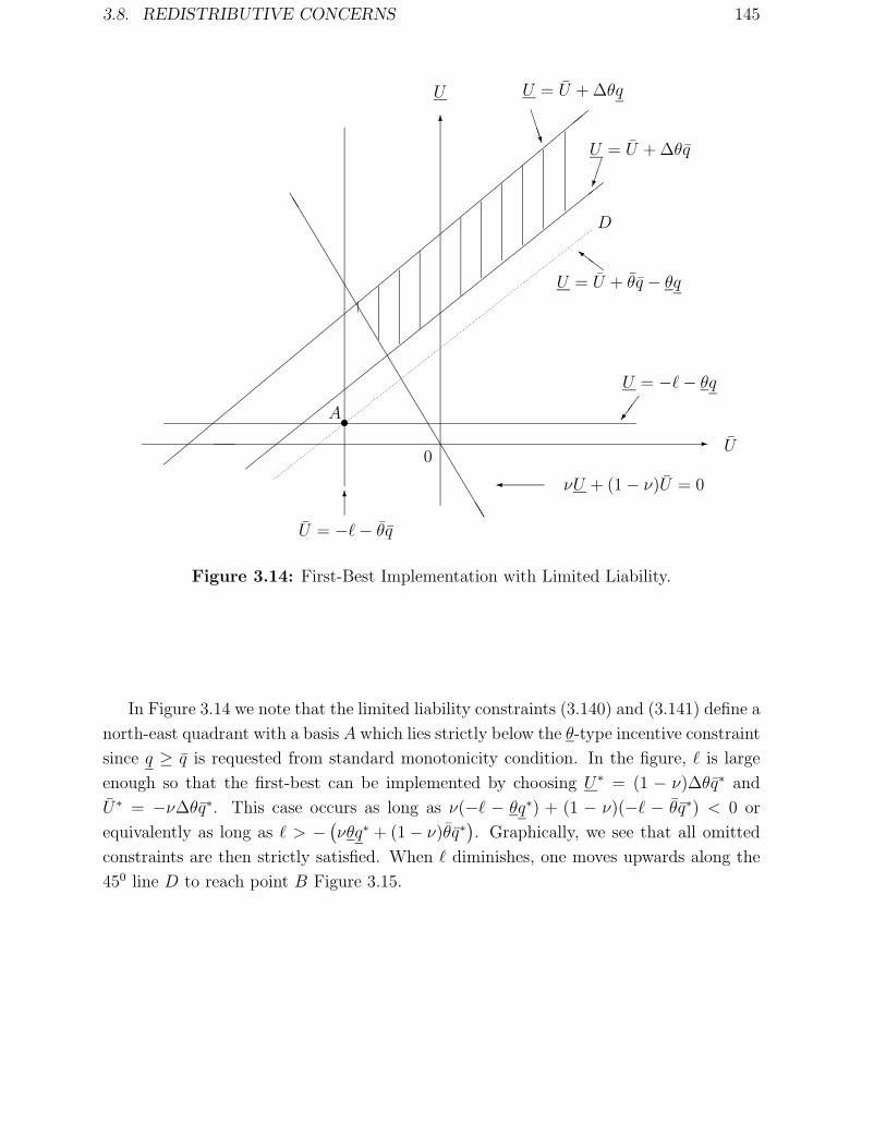
3.8. REDISTRIBUTIVE CONCERNS 145
6
-0
U
U#
##
##
##
##
##
##
##
##
##
##
##
##
,,
,,
,,
,,
,,
,,
,,
,,
,,
,,
,,
,,
,,
,,
,,
•A
U = U + ∆θq
BBBN
U = U + ∆θq££°
U = U + θq − θqZZ}
U = −`− θq
¶¶/
νU + (1− ν)U = 0¾
U = −`− θq
6
D
TT
TT
TT
TT
TT
TT
TT
TT
TT
TTTTTT
Figure 3.14: First-Best Implementation with Limited Liability.
In Figure 3.14 we note that the limited liability constraints (3.140) and (3.141) define a
north-east quadrant with a basis A which lies strictly below the θ-type incentive constraint
since q ≥ q is requested from standard monotonicity condition. In the figure, ` is large
enough so that the first-best can be implemented by choosing U∗ = (1 − ν)∆θq∗ and
U∗ = −ν∆θq∗. This case occurs as long as ν(−` − θq∗) + (1 − ν)(−` − θq∗) < 0 or
equivalently as long as ` > − (νθq∗ + (1− ν)θq∗
). Graphically, we see that all omitted
constraints are then strictly satisfied. When ` diminishes, one moves upwards along the
450 line D to reach point B Figure 3.15.

146 CHAPTER 3. INCENTIVE AND PARTICIPATION CONSTRAINTS
6
-0
U
U#
##
##
##
##
##
##
##
##
##
##
##
##
,,
,,
,,
,,
,,
,,
,,
,,
,,
,,
,,
,,
,,
,,
,,
U = U + ∆θq
BBBN
U = U + ∆θq££°
U = U + θq − θqZZ}
νU + (1− ν)U = 0¾
D
@@
@@
@@
@@
@@
@@
@@
@@
@@
@@
@@
•
B
U = −`− θqS
SSSw
U = −`− θq
?
BBBB
BBBB
BBBB
BBBBB
BBBB
BBBBB
BBBB
BBBBB
BBBBB
BBBBB
BBBBB
BBBBB
LLLLL
AAAA
AAAA
Figure 3.15: Distortion with Limited Liability.
In Figure 3.15, we see that (3.76), (3.79) and (3.80) are all binding. In this case, we
obtain UL = ∆θqL−`− θqL, UL = −`− θqL and ` = −θqL +ν∆θqL = −(νθ+(1−ν)θ)qL.
This solution entails a distortion of a θ-agent’s output. It is valid as long as qL ≤ q∗ to
keep the usual monotonicity condition satisfied. Finally, when ` < −(νθ + (1 − ν)θ)q∗,both types are bunched together and produce q such that ` = −(νθ + (1− ν)θ)q.

Chapter 4
Moral Hazard: The Basic Trade-Offs
4.1 Introduction
In the introduction to Chapter 2, we have stressed that the delegation of task creates an
information gap between the principal and his agent when the latter may have learned
some piece of information relevant for determining the efficient volume of trade. Adverse
selection is not the only informational problem one can imagine. Agents to whom a task
has been delegated by a principal may also choose actions which affect the value of trade
or, more generally, the agent’s performance. By the mere fact of delegation, the principal
loses any ability to control those actions when those actions are no longer observable,
either by the principal who offers the contract, or by the Court of Justice which enforces
it. Those actions cannot be contracted upon because no one can verify the value of the
agent’s actions. We will then say that there is moral hazard.1
The leading candidates for such moral hazard actions are effort variables which influ-
ence positively the agent’s level of production but also create a disutility for the agent.
For instance, the yield of a field depends on the amount of time that the tenant has spent
selecting the good crops, or the quality of the harvesting he has made. Similarly, the
probability that a driver gets a car crash depends on how safely he drives and this affects
his demand for insurance. Also, a regulated firm may have to perform a costly and non
observable investment to reduce its cost of producing a socially valuable good. However,
the agent’s action can also be a more complex array of decisions which defines the agent’s
task or his job attributes. The agent can sometimes choose among various projects to be
carried out on behalf of the principal with each project being associated with a particular
non-transferable private benefit that he may get if this project is selected. As an example,
the manager of a large corporation may divert the firm’s resources in perquisites rather
1This situation is sometimes also referred to as hidden action. See Section 1.7 for the origin of theexpression moral hazard.
147

148 CHAPTER 4. MORAL HAZARD: THE BASIC TRADE-OFFS
than in hiring new engineers for the firm’s research lab.
It is important to stress that, as adverse selection, moral hazard would not be an issue
if the principal and the agent had the same objective function. Crucial to the agency cost
arising under moral hazard is the conflict between the principal and the agent over which
action should be carried out. The non-observability of the agent’s action may then prevent
an efficient resolution of this conflict of interest since a contract can never stipulate which
action should be taken by the agent.
As under adverse selection, asymmetric information plays here also a crucial role in
the design of the incentive contract under moral hazard. However, instead of being an
exogenous uncertainty for the principal, uncertainty is now endogenous. The probabilities
of the different states of nature and thus the expected volume of trade depend now
explicitly on the agent’s effort. In other words, the realized production level is only a noisy
signal of the agent’s action. This uncertainty is key to understand the contractual problem
under moral hazard. Had the mapping between effort and performance been completely
deterministic, the principal and the Court of Justice would have no difficulties in inferring
the agent’s effort from the observed output. Even if effort is non-observable directly,
it could be indirectly contracted upon since output is itself observable and verifiable.
The non-observability of the effort would not put any real constraint on the principal’s
ability to contract with the agent and their conflict of interest would be costless to solve.
Contrary to what occurs in the adverse selection paradigm, the resolution of uncertainty
is now common knowledge ex post and contracting takes place before output realizes, i.e.,
at the ex ante stage.
In a moral hazard context, the random output aggregates the agent’s effort and the
realization of pure luck. However, the principal can only design a contract based on the
agent’s observable performance. Through this contract, the principal wants to induce,
at a reasonable cost, a good action of the agent despite the impossibility to condition
directly the agent’s reward on his action. In general, the non-observability of the agent’s
effort affects the cost of implementing a given action. To illustrate this point, we present
a model where a risk averse agent can choose a binary effort, and the production level
can be either high or low. A first step of the analysis made in this chapter is to study
the properties of incentive schemes which induce a positive and costly effort. Such a
scheme must thus satisfy an incentive constraint. Also, inducing the agent’s voluntary
participation imposes a standard participation constraint. Incentive feasible contracts are
those satisfying those two constraints. Among such schemes, the principal prefers the one
which implements the positive level of effort at minimal cost. This cost minimization yields
the characterization of the second-best cost of implementing this effort. In general, this
second-best cost is greater than the first-best cost which would be obtained by assuming
that effort is verifiable. The reason is that an incentive constraint is generally binding for

4.1. INTRODUCTION 149
the incentive scheme implementing a positive effort at minimal cost.
Once this first step of the analysis is performed, we can characterize the second-
best effort chosen by the principal. This second-best effort trades-off the benefit for the
principal of inducing a given effort against the second-best cost of implementing this
effort. The main lesson of this second step of the analysis is that the second-best effort
may differ from the first-best one. An allocative inefficiency emerges as the result of the
conflict of interest between the principal and the agent.
Let us now see in more detail the terms of the moral hazard trade-offs. When the
agent is risk neutral, the non-observability of effort has no bite on the efficiency of trade.
Moral hazard does not create any transaction cost. The principal can achieve the same
utility level as if he could directly control the agent’s effort. This first-best outcome is
nevertheless obtained through a contract which is contingent on the level of production.
The agent is incentivized by being rewarded for good production levels and penalized
otherwise. Since the agent is risk neutral, he is ready to accept penalties and rewards
as long as the expected payment he receives satisfies his ex ante participation constraint.
Transfers can be structured to saturate the agent’s participation constraint while inducing
the desirable effort level. One way of doing so is to make the agent residual claimant for
the gains from trade and to grasp from him this gain through an ex ante lump-sum
transfer.
If the risk neutral agent has no wealth and cannot be punished, a new limited liability
constraint must be satisfied on top of the usual incentive and participation constraint.
There is then a conflict between the limited liability and the incentive constraints. Indeed,
punishment being infeasible, the principal is restricted to use only rewards to induce
effort. This restriction in the principal’s instruments implies that he must give up some
ex ante rent to the agent. This limited liability rent is costly for the principal who then
distorts the second-best effort level below its first-best value to reduce the cost of this
rent. As for adverse selection and ex post participation constraints, we have a quite similar
limited liability rent extraction-efficiency trade-off leading to a downward distortion in the
expected volume of trade.
If the agent is risk averse, a constant wage provides full insurance but induces no
effort provision. Inducing effort requires to let the agent bear some risk. To accept such
a risky contract, the agent must receive a risk premium. There is now a conflict between
the incentive and the participation constraints. This leads to an insurance-efficiency
trade-off. To solve this trade-off, the principal must distort the complete information risk
sharing agreement between him and the agent to induce effort provision. As we will see
in Chapter 5 below, there is no general lesson on how the second-best and the first-best
effort can be compared in a moral hazard environment. However, in a model with two

150 CHAPTER 4. MORAL HAZARD: THE BASIC TRADE-OFFS
effort levels, one can still easily show that a high effort is less often implemented by the
principal than under complete information.
In Section 4.2, we present the general moral hazard model highlighting the stochastic
nature of the production process in a two-effort-two-outcome setting. We also describe
there the set of incentive feasible contracts inducing a high level of effort and we derive
as a benchmark the first-best decision rule. In Section 4.3, we show that the agent’s
risk neutrality imposes no real transaction cost on the efficiency of contracting. Section
4.4 focuses on the trade-off between extraction of the limited liability rent and allocative
efficiency under risk neutrality. Section 4.5 deals with the trade-off between insurance
and efficiency under risk aversion. These latter two sections are the core of the chapter.
We then extend the basic framework to provide various comparative statics results on
the optimal contract. In Section 4.6, we briefly generalize our previous insights to the
case of more than two levels of performance. This extension is worth pursuing to analyze
the conditions on the information structure which ensure the monotonicity of the agent’s
compensation schedule. In Section 4.7, we investigate the properties of various information
systems from an agency point of view. We prove there an important property: any
signal which is informative on the agent’s effort should be included as an argument of his
compensation payment. Section 4.8 proposes a brief overview of the insights obtained from
the moral hazard paradigm to understand the theory of the firm. Section 4.9 develops
a number of bareboned examples where the moral hazard paradigm has proved to be
extremely useful.
4.2 The Model
4.2.1 Effort and Production
We consider an agent who can exert a costly effort e. e can take two possible values
that we normalize respectively as a zero effort level and a positive effort of one: e in
{0, 1}. Exerting effort e implies a disutility for the agent which is equal to ψ(e) with the
normalizations ψ(0) = ψ0 = 0 and ψ(1) = ψ1 = ψ.
The agent receives a transfer t from the principal and we assume that his utility func-
tion is separable between money and effort2, U = u(t)− ψ(e), with u(·) being increasing
and concave (u′(·) > 0, u′′(·) < 0). Sometimes, we will use the function h = u−1, the
inverse function of u(·), which is also increasing and convex (h′(·) > 0, h′′(·) > 0).
Production is stochastic and effort affects the production level as follows. The stochas-
2This assumption facilitates notations and is irrelevant in this chapter. See Chapter 5 for the case ofnon-separability and its possible impact on the main features of the optimal contract.

4.2. THE MODEL 151
tic production level q can only take two values {q, q}, with q − q = ∆q > 0, and the
stochastic influence of effort on production is characterized by the probabilities Pr(q =
q/e = 0) = π0, and Pr(q = q/e = 1) = π1, with π1 > π0. We will denote by ∆π = π1 − π0
the difference between these two probabilities.
Note that effort improves production in the first-order stochastic dominance sense,
i.e., Pr(q ≤ q∗|e) is decreasing with e for any given production q∗. Indeed, we have:
Pr(q ≤ q|e = 1) = 1− π1 < 1− π0 = Pr(q ≤ q|e = 0) and Pr(q ≤ q|e = 1) = 1 = Pr(q ≤q|e = 0). This property implies that any principal who has an utility function v(·) which
is increasing in production prefers the stochastic distribution of production induced by
the positive effort level e = 1 to that induced by the null effort e = 0. Indeed, we have:
π1v(q)+(1−π1)v(q) = π0v(q)+(1−π0)v(q)+(π1−π0)(v(q)−v(q)) which is greater than
π0v(q) + (1− π0)v(q) if v(·) is increasing. So, an increase in effort improves production in
a strong sense in this model with two possible levels of performance.
4.2.2 Incentive Feasible Contracts
Mimicking what we did in Chapters 2 and 3, we now describe incentive feasible contracts
in a moral hazard environment. In such an environment, the agent’s action is not directly
observable by the principal. The principal can only offer a contract based on the observable
and verifiable production level, i.e., a function {t(q)} linking the agent’s compensation to
the random output q. With two possible outcomes q and q, the contract can equivalently
be defined by a pair of transfers t and t. t (resp. t) is the payment received by the agent
if the production q (resp. q) realizes. Keeping the same notations as in Chapter 2, the
risk neutral principal’s expected utility writes now as:
V1 = π1(S(q)− t) + (1− π1)(S(q)− t), (4.1)
if the agent makes a positive effort (e = 1), and
V0 = π0(S(q)− t) + (1− π0)(S(q)− t), (4.2)
if the agent makes no effort (e = 0). For notational simplicity, we will denote all along
this chapter the principal’s benefits in each state of nature respectively by S(q) = S and
S(q) = S.
The problem of the principal is now to decide whether to induce the agent to exert
effort or not, and if he chooses to do so, which incentive contract should be used.
To each level of effort that the principal wishes to induce corresponds a set of contracts
ensuring participation and incentive compatibility. In our model with two possible levels
of effort, we will say that a contract is incentive feasible if it induces a positive effort and

152 CHAPTER 4. MORAL HAZARD: THE BASIC TRADE-OFFS
ensures the agent’s participation. The corresponding moral hazard incentive constraint
writes thus as:
π1u(t) + (1− π1)u(t)− ψ ≥ π0u(t) + (1− π0)u(t). (4.3)
(4.3) is the incentive constraint which imposes that the agent prefers to exert a positive
effort. If he exerts effort, the agent faces the lottery which gives t (resp. t) with probability
π1 (resp. 1 − π1) and not the lottery which yields t (resp. t) with probability π0 (resp.
1 − π0). However, when he does not exert effort, the agent incurs no disutility of effort
and saves an amount ψ.
Still normalizing at zero the agent’s reservation utility, the agent’s participation con-
straint writes now as:
π1u(t) + (1− π1)u(t)− ψ ≥ 0. (4.4)
(4.4) is the agent’s participation constraint requiring that exerting effort yields to the
agent at least his outside opportunity utility level. Note that this participation constraint
is ensured at the ex ante stage, i.e., before the realization of the production shock.3
Definition 4.1 : An incentive feasible contract satisfies the incentive and participation
constraints (4.3) and (4.4).
Finally, the timing of the contracting game under moral hazard can be summarized
as follows:
-? ??? ?
t = 0 t = 1 t = 2 t = 3 t = 4
Poffers a contract
{(t, t)}.
Aaccepts
or refusesthe contract
Aexerts an
effort or not
The outcome q
is realizedThe contractis executed
time
Figure 4.1: Timing of Contracting under Moral Hazard.
3See Section 2.12 for the case of ex ante contracting under adverse selection.

4.2. THE MODEL 153
4.2.3 The Complete Information Optimal Contract
As a benchmark, let us first assume that the principal and a benevolent Court of Justice
can observe effort and that this variable is now observable and verifiable and can thus be
included into a contract enforced by this Court. Then, if he wants to induce effort, the
principal’s problem becomes:
(P ) : max{(t,t)}
π1(S − t) + (1− π1)(S − t)
subject to (4.4).
Indeed, only the agent’s participation constraint matters for the principal since the
agent can be forced to exert the positive level of effort. If the agent were not choosing this
level of effort, the agent’s deviation could be perfectly detected by both the principal and
the Court of Justice. The agent could be heavily punished and the Court could enforce
such a punishment.
Denoting by λ the multiplier of this participation constraint and optimizing with
respect to t and t yields respectively the following first-order conditions:
−π1 + λπ1u′(t∗) = 0, (4.5)
−(1− π1) + λ(1− π1)u′(t∗) = 0, (4.6)
where t∗ and t∗ are the first-best transfers.
From (4.5) and (4.6) we immediately derive that λ = 1u′(t∗) = 1
u′(t∗) > 0, and finally
that t∗ = t∗ = t∗.
With a verifiable effort, the agent obtains therefore full insurance from the risk neutral
principal and the transfer t∗ he receives is the same whatever the state of nature. Since
the participation constraint is binding, we also obtain the value of this transfer which is
just enough to cover the disutility of effort, namely t∗ = h(ψ). This is also the expected
payment made by the principal to the agent or the first-best cost CFB of implementing
the positive effort level. For the principal, inducing effort yields therefore an expected
payoff equal to:
V1 = π1S + (1− π1)S − h(ψ). (4.7)
Had the principal decided to let the agent exert no effort, e = 0, he would make a zero
payment to the agent whatever the realization of output. Thereby, the principal would
obtain instead a payoff:
V0 = π0S + (1− π0)S. (4.8)

154 CHAPTER 4. MORAL HAZARD: THE BASIC TRADE-OFFS
Inducing effort is thus optimal from the principal’s point of view when V1 ≥ V0, i.e.:
π1S + (1− π1)S − h(ψ) ≥ π0S + (1− π0)S, or to put it differently when:
∆π∆S︸ ︷︷ ︸Expected
gainof effort
≥ h(ψ)︸︷︷︸first-best costof inducing
effort
, (4.9)
where ∆S = S − S > 0.
The left-hand side of (4.9) captures the gain of increasing effort from e = 0 to e = 1.
This gain comes from the fact that the return S, which is greater than S, arises more
often when a positive effort is exerted. The right-hand side of (4.9) is instead the first-best
cost of inducing the agent’s acceptance when he exerts a positive effort.
Denoting by B = ∆π∆S the benefit of inducing a strictly positive effort level, the
first-best outcome calls for e∗ = 1 if and only if B ≥ h(ψ) as shown in Figure 4.2.
¾-¾e∗ = 0 e∗ = 1
CFB = h(ψ)
-
-
First-Best Effort
Benefit
e
B
Figure 4.2: First-Best Level of Effort.
4.3 Risk Neutrality and First-Best Implementation
If the agent is risk neutral, we have (up to an affine transformation) u(t) = t for all t
and h(u) = u for all u. The principal who wants to induce effort must thus choose the
contract which solves the following problem:
(P ) : max{(t,t)}
π1(S − t) + (1− π1)(S − t)
π1t + (1− π1)t− ψ ≥ π0t + (1− π0)t (4.10)
π1t + (1− π1)t− ψ ≥ 0. (4.11)
With risk neutrality, the principal can for instance choose incentive compatible trans-
fers t and t which saturate the agent’s participation constraint and leave no rent to the
agent. Indeed, solving (4.10) and (4.11) with equalities, we obtain immediately:
t∗ = − π0
∆πψ, (4.12)

4.3. RISK NEUTRALITY AND FIRST-BEST IMPLEMENTATION 155
and
t∗ =1− π0
∆πψ. (4.13)
The agent is rewarded if production is high. His net utility in this state of nature
U∗ = t∗ − ψ is then U∗ = 1−π1
∆πψ > 0. The agent is instead punished if production is low.
His corresponding net utility U∗ = t∗ − ψ is thus U∗ = − π1
∆πψ < 0.
The principal (who is risk neutral with respect to transfers) makes an expected pay-
ment π1t∗ + (1 − π1)t
∗ = ψ which is equal to the disutility of effort he would incur if he
could perfectly control the effort level or if he was carrying the agent’s task himself. The
principal can costlessly structure the agent’s payment so that the latter has the right in-
centives to exert effort. Indeed, by increasing effort from e = 0 to e = 1, the agent receives
more often the transfer t∗ than the transfer t∗. Using (4.12) and (4.13), his expected gain
from exerting effort is thus ∆π(t∗− t∗) = ψ, i.e., it exactly compensates the agent for the
extra disutility of effort that the agent incurs when increasing his effort from e = 0 to
e = 1.
Delegation is here costless to the principal. Therefore, if effort is socially valuable in
the first-best world, it will also be implemented by the principal with the incentive scheme
{(t∗, t∗)} when effort is no longer observed by the principal and the agent is risk neutral.
Summarizing, we have:
Proposition 4.1 : Moral hazard is not an issue with a risk neutral agent despite the
non-observability of effort. The first-best level of effort is still implemented.
Remark 1: The reader will have recognized the similarity of those results with those
described in Section 2.12. In both cases, when contracting takes place ex ante, i.e.,
before the realization of the state of nature, the incentive constraint, either under adverse
selection, or now under moral hazard, does not conflict with the ex ante participation
constraint with a risk neutral agent and the first-best outcome is still implemented.
Remark 2: The transfers (t∗, t∗) defined in (4.12) and (4.13) yield only one possible
implementation of the first-best outcome, an implementation such that the incentive con-
straint (4.10) is exactly binding. Other pairs of transfers can be used which may induce
a strict preference of the agent for exerting effort.
Let us for instance consider the following transfers t∗′= S − T ∗, and t∗
′= S − T ∗,
where T ∗ is an upfront payment made by the agent before output realizes. Those transfers
satisfy the agent’s incentive constraint since:
∆π(t∗′ − t∗
′) = ∆π∆S > h(ψ) = ψ (4.14)

156 CHAPTER 4. MORAL HAZARD: THE BASIC TRADE-OFFS
where the right-hand side inequality comes from the fact that effort is socially optimal in
a first-best world. Moreover, the upfront payment T ∗ can be adjusted by the principal to
have the agent’s participation constraint binding. The corresponding value of this transfer
is T ∗ = π1S + (1 − π1)S − ψ. With the transfers t∗′
and t∗′
above, the agent becomes
residual claimant for the profit of the firm. T ∗ is thus precisely equal to this expected
profit. The principal requires this ex ante payment to reap all gains from delegation.
Making the risk neutral agent residual claimant for the hierarchy’s profit is an optimal
response to the moral hazard problem. In other words the principal must sell the property
rights over the firm to the agent. Indeed a proper allocation of property rights is sufficient
to induce efficiency.4
On the contrary, inefficiencies in effort provision due to moral hazard will arise when
the agent is no longer risk neutral. There are two alternative ways to model these trans-
action costs. One is to maintain risk neutrality for positive income levels, but impose
a limited liability constraint, which requires transfers not to be too negative. The other
is to let the agent be strictly risk averse. We analyze in turn those two contractual
environments and the different trade-offs they respectively imply.
4.4 The Trade-Off between Limited Liability Rent
Extraction and Efficiency
Let us thus consider a risk neutral agent. As we have already seen, (4.3) and (4.4) take
now the following forms:
π1t + (1− π1)t− ψ ≥ π0t + (1− π0)t, (4.15)
and
π1t + (1− π1)t− ψ ≥ 0. (4.16)
Let us also assume that the agent’s transfer must always be greater than some ex-
ogenous level −` with ` ≥ 0. The framework is thus quite similar to that of Section 3.6,
and we refer to that section for some motivations and discussions of the origins of such
limited liability constraints on transfers. Limited liability constraints in both states of
nature write thus as:
t ≥ −`, (4.17)
4See Tirole (1999) for a more general discussion of when a proper allocation of property rights imple-ments the optimal contract. See also Section 5.3.5.
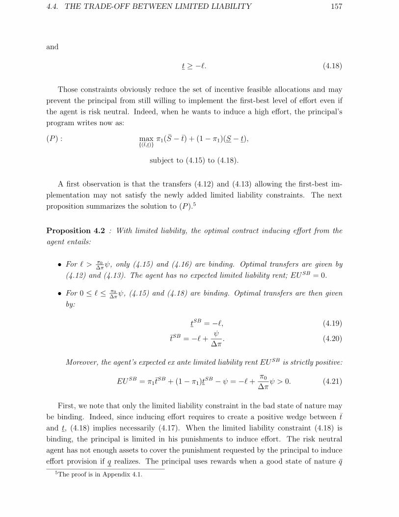
4.4. THE TRADE-OFF BETWEEN LIMITED LIABILITY 157
and
t ≥ −`. (4.18)
Those constraints obviously reduce the set of incentive feasible allocations and may
prevent the principal from still willing to implement the first-best level of effort even if
the agent is risk neutral. Indeed, when he wants to induce a high effort, the principal’s
program writes now as:
(P ) : max{(t,t)}
π1(S − t) + (1− π1)(S − t),
subject to (4.15) to (4.18).
A first observation is that the transfers (4.12) and (4.13) allowing the first-best im-
plementation may not satisfy the newly added limited liability constraints. The next
proposition summarizes the solution to (P ).5
Proposition 4.2 : With limited liability, the optimal contract inducing effort from the
agent entails:
• For ` > π0
∆πψ, only (4.15) and (4.16) are binding. Optimal transfers are given by
(4.12) and (4.13). The agent has no expected limited liability rent; EUSB = 0.
• For 0 ≤ ` ≤ π0
∆πψ, (4.15) and (4.18) are binding. Optimal transfers are then given
by:
tSB = −`, (4.19)
tSB = −` +ψ
∆π. (4.20)
Moreover, the agent’s expected ex ante limited liability rent EUSB is strictly positive:
EUSB = π1tSB + (1− π1)t
SB − ψ = −` +π0
∆πψ > 0. (4.21)
First, we note that only the limited liability constraint in the bad state of nature may
be binding. Indeed, since inducing effort requires to create a positive wedge between t
and t, (4.18) implies necessarily (4.17). When the limited liability constraint (4.18) is
binding, the principal is limited in his punishments to induce effort. The risk neutral
agent has not enough assets to cover the punishment requested by the principal to induce
effort provision if q realizes. The principal uses rewards when a good state of nature q
5The proof is in Appendix 4.1.

158 CHAPTER 4. MORAL HAZARD: THE BASIC TRADE-OFFS
realizes. As a result, the agent receives a strictly positive ex ante limited liability rent
described by (4.21). Comparing with the case without limited liability this rent is actually
the additional payment that the principal must incur because of the conjunction of moral
hazard and limited liability.
As the agent is endowed with more assets, i.e., as ` gets larger, the conflict between
moral hazard and limited liability diminishes and disappears whenever ` is large enough.
In this case, the agent avoids bankruptcy even when he has to pay the principal in the
bad state of nature.
Let us now assume that ` = 0 so that only positive transfers are feasible. We model
therefore a contractual environment where the agent owns no asset at the time of starting
the relationship with the principal. When he induces effort from the agent, the principal’s
expected utility can be computed as:
V SB1 = π1S + (1− π1)S − π1ψ
∆π. (4.22)
If the principal gives up the goal of inducing effort from the agent, he can choose
t = t = 0 and obtain instead the expected utility level (4.8). It is worth inducing effort if
V SB1 is greater than V0, i.e., when:
∆π∆S ≥ π1ψ
∆π. (4.23)
The left-hand side of (4.23) is the gain of inducing effort, i.e., the gain of increasing the
probability of a high production level. The right-hand side is instead the second-best cost
CSB of inducing effort which is the disutility of effort ψ plus now the limited liability rentπ0ψ∆π
. This second-best cost of implementing effort obviously exceeds the first best cost. As
it can easily been seen by comparing (4.23) and the right-hand side of (4.9) (taken for the
case of risk neutrality, i.e., for h(ψ) = ψ), limited liability and moral hazard altogether
make costlier to induce effort.
Figure 4.3 below describes the reduced subset of values of B justifying a high effort
from the agent when limited liability and moral hazard interact.
-¾-
¾-
eSB = 1eSB = 0
e∗ = 0 e∗ = 1
CFB = ψ CSB = π1ψ∆π
First-Best Effort
Second-Best EffortBenefit
-
-
Figure 4.3: First- and Second-Best Efforts with Moral Hazard and Limited Liability.

4.5. THE TRADE-OFF BETWEEN INSURANCE AND EFFICIENCY 159
Moral hazard justifies an underprovision of effort when the benefit B of a strictly
positive effort lies between ψ and π1
∆πψ. Summarizing our analysis, we have:
Proposition 4.3 : With moral hazard and limited liability, there is a trade-off between
inducing effort and giving up an ex ante limited liability rent to the agent. The principal
chooses less often to induce a high effort from the agent.
4.5 The Trade-Off Between Insurance and Efficiency
Let us now turn to the second source of inefficiency in a moral hazard context: the agent’s
risk aversion. When the agent is risk averse, the principal’s program writes now as:
(P ) : max{(t,t)}
π1(S − t) + (1− π1)(S − t),
subject to (4.3) and (4.4).
It is not obvious that (P ) is a concave program for which the first-order Kuhn and
Tucker conditions are necessary and sufficient. The reason for this possible lack of concav-
ity is that the concave function u(·) appears on both sides of the incentive compatibility
constraint (4.3). However, the following change of variables shows that concavity of the
program is ensured. Let us define u = u(t) and u = u(t) or equivalently let t = h(u) and
t = h(u). These new variables are the levels of ex post utility obtained by the agent in
both states of nature. The set of incentive feasible contracts can now be described by two
linear constraints:
π1u + (1− π1)u− ψ ≥ π0u + (1− π0)u, (4.24)
which replaces the incentive constraint (4.3) and also
π1u + (1− π1)u− ψ ≥ 0, (4.25)
which replaces the participation constraint (4.4).
Program (P ) can now be replaced by a new program (P ′) which writes as:
(P ′) : max{(u,u)}
π1(S − h(u)) + (1− π1)(S − h(u))
subject to (4.24) and (4.25).
Note that the principal’s objective function is now strictly concave in (u, u) since h(·)is strictly convex. The constraints being linear, (P ′) is thus a concave problem with
the Kuhn and Tucker conditions being both sufficient and necessary for characterizing
optimality.

160 CHAPTER 4. MORAL HAZARD: THE BASIC TRADE-OFFS
4.5.1 Optimal Transfers
Letting λ and µ be the non-negative multipliers associated respectively with constraints
(4.24) and (4.25), the first-order conditions of this program can be expressed respectively
as:
−π1h′(uSB) + λ∆π + µπ1 = − π1
u′(tSB)+ λ∆π + µπ1 = 0, (4.26)
−(1− π1)h′(uSB)− λ∆π + µπ1 = −(1− π1)
u′(tSB)− λ∆π + µ(1− π1) = 0, (4.27)
where tSB and tSB are the second-best optimal transfers. Rearranging terms, we get:
1
u′(tSB)= µ + λ
∆π
π1
, (4.28)
1
u′(tSB)= µ− λ
∆π
1− π1
. (4.29)
The four variables (tSB, tSB, λ, µ) are simultaneously obtained as the solution to the
system of four equations (4.24), (4.25), (4.28) and (4.29). Multiplying (4.28) by π1 and
(4.29) by 1− π1 and adding those two modified equations, we obtain:
µ =π1
u′(tSB)+
1− π1
u′(tSB)> 0. (4.30)
Hence, the participation constraint (4.25) is necessarily binding.
Using (4.30) and (4.28), we obtain also:
λ =π1(1− π1)
∆π
(1
u′(tSB)− 1
u′(tSB)
). (4.31)
λ must also be strictly positive. Indeed, from (4.24), we have uSB − uSB ≥ ψ∆π
> 0,
and thus tSB > tSB implying that the right-hand side of (4.31) is strictly positive since
u′′ < 0.
Henceforth, the risk averse agent does not receive full insurance anymore. This result
must be contrasted with what we have seen under complete information in Section 4.2.3.
Indeed, with full insurance, the incentive compatibility constraint (4.3) can no longer be
satisfied. Inducing effort requires to let the agent bear some risk. Summarizing, we can
state:
Proposition 4.4 : When the agent is strictly risk averse, the optimal contract which
induces effort saturates both the agent’s participation and incentive constraints. This
contract does not provide full insurance. Moreover, second-best transfers are obtained as:
tSB = h
(ψ + (1− π1)
ψ
∆π
), (4.32)

4.5. THE TRADE-OFF BETWEEN INSURANCE AND EFFICIENCY 161
and
tSB = h
(ψ − π1
ψ
∆π
). (4.33)
It is also worth noting that the agent receives more than the complete information
transfer when a high output realizes, tSB > h(ψ). When a low output realizes, the agent
receives instead less than the complete information transfer, tSB < h(ψ). A risk premium
must be paid to the risk averse agent to induce his participation since he incurs now a
risk coming from the fact that tSB < tSB. Indeed, when (4.4) is binding, we have:
ψ = π1u(tSB) + (1− π1)u(tSB) < u(π1tSB + (1− π1)t
SB), (4.34)
where the right-hand side inequality in (4.34) follows from Jensen’s inequality. The ex-
pected payment π1tSB +(1−π)tSB given by the principal is thus larger than the first-best
cost CFB1 = h(ψ) which is incurred by the principal when effort is observable as we have
seen in Section 4.2.3.
4.5.2 Optimal Second-Best Effort
Let us now turn to the question of the second-best optimality of inducing a high effort
from the principal’s point of view. The second-best cost CSB of inducing effort under
moral hazard is the expected payment made to the agent CSB = π1tSB + (1 − π1)t
SB.
Using (4.32) and (4.33), this cost rewrites as:
CSB = π1h
(ψ + (1− π1)
ψ
∆π
)+ (1− π1)h
(ψ − π1ψ
∆π
). (4.35)
The benefit of inducing effort is still B = ∆π∆S and a positive effort e∗ = 1 is the
optimal choice of the principal whenever:
∆π∆S ≥ CSB = π1h
(ψ + (1− π1)
ψ
∆π
)+ (1− π1)h
(ψ − π1ψ
∆π
). (4.36)
h(·) being strictly convex, Jensen’s inequality implies that the right-hand side of (4.36)
is strictly greater than the first-best cost of implementing effort CFB = h(ψ). Therefore,
inducing a high effort occurs less often with moral hazard than when effort is observable.
Figure 4.4 represents this phenomenon graphically.

162 CHAPTER 4. MORAL HAZARD: THE BASIC TRADE-OFFS
-
CFB CSB
Benefit
e∗ = 0 e∗ = 1
eSB = 0 eSB = 1Second-Best Effort
First-Best Effort
B
- ¾
¾-
-
-
Figure 4.4: Second-Best Level of Effort with Moral Hazard and Risk Aversion.
For B belonging to the interval [CFB, CSB], the second-best level of effort is zero and
is thus strictly below its first-best value. There is now under-provision of effort because
of moral hazard and risk aversion.
Proposition 4.5 : With moral hazard and risk aversion, there is a trade-off between
inducing effort and providing insurance to the agent. The principal induces less often a
positive effort from the agent than with risk neutrality.
To get further insights on the dependency of the second-best cost of implementation
on various parameters, let us thus specialize the model and assume that h(u) = u + ru2
2
where r > 0.6 Equivalently, this means that u(x) = −1+√
1+2rxr
. From (4.35), we have now
the following expression of CSB:
CSB = ψ +rψ2
2+
rψ2π1(1− π1)
2(∆π2). (4.37)
The first-best cost of implementing effort with such a utility function would instead
be:
CFB = ψ +rψ2
2. (4.38)
Henceforth, the agency cost AC, which is also the principal’s loss between his first-best
and his second-best expected profit when he implements a positive effort in both cases
can be defined as:
AC = CSB − CFB =rψ2π1(1− π1)
2(∆π)2. (4.39)
This agency cost increases with r, a measure of the agent’s degree of risk aversion, with
ψ the cost of one unit of effort, and with η = π1(1−π1)∆π
. η is a measure of the informational
6This quadratic specification can be viewed as a reasonable approximation of any inverse functionh(u) whenever u is small enough. Note that r can then be considered as the agent’s degree of absoluterisk aversion around zero.

4.6. MORE THAN TWO LEVELS OF PERFORMANCE 163
problem for the principal. Everything else being kept equal, it becomes harder, and less
often optimal for the principal, to induce a high effort as η increases. η is larger when π1 is
close to 12. In this case, the variance of the measured performance q is the greatest possible
one: the observable output is a rather poor indicator of the agent’s effort. Therefore, more
noisy measures of the agent’s effort will more often call for inducing a low effort at the
optimum and for a fixed wage without any incentives being provided. Finally, note that
η is also larger when ∆π is small, i.e., when the difference in utilities u(tSB) − u(tSB)
necessary to incentivize the agent gets larger. More generally, this dependence of the
agency cost on η shows that the informational content of the observable output plays a
crucial role in the design of the optimal contract. This is a general theme of agency theory
that we will cover more extensively in Section 4.7 below.
4.6 More Than Two Levels of Performance
We now extend our previous models to allow for more than two levels of performance.7
We consider a production process where n possible outcomes can be realized. Those
performances can be ordered so that q1 < q2 . . . < qi < . . . < qn. We denote also
by Si = S(qi) the principal’s return in each of those states of nature. In this context,
a contract is a n-uple of payments {(t1, . . . , tn)}. Let also πik be the probability that
production qi takes place when the effort level is ek. We assume that πik > 0 for all pairs8
(i, k) with∑n
i=1 πik = 1. Finally, we keep the assumption that only two possible levels of
effort are feasible, i.e., ek in {0, 1}. We still denote ∆πi = πi1 − πi0.
4.6.1 Limited Liability
Consider first the limited liability model of Section 4.4. The optimal contract inducing a
positive effort must now solve the following program:
(P ) : max{(t1,... ,tn)}
n∑i=1
πi1(Si − ti)
subject to
n∑i=1
πi1ti − ψ ≥ 0, (4.40)
7See Appendix 4.2 for the case of a continuum of performances.8Mirrlees (1999) has shown that if the support of probabilities varies with the level of effort, then the
first-best can be achieved. This is because there is then a non zero probability that the agent revealsthat he has not taken the postulated effort level and he can be punished strongly in that case.

164 CHAPTER 4. MORAL HAZARD: THE BASIC TRADE-OFFS
n∑i=1
(πi1 − πi0)ti ≥ ψ, (4.41)
ti ≥ 0, for all i in {1, . . . , n}. (4.42)
(4.40) is the agent’s participation constraint. (4.41) is his incentive constraint. (4.42)
are all the limited liability constraints that we simplify, with respect to Section 4.4, by
assuming that the agent cannot be inflicted a negative payment, i.e., the agent has no
asset of his own before starting the relationship with the principal.
First, note that the participation constraint (4.40) is implied by the incentive (4.41)
and the limited liability constraints (4.42). Indeed, we have:
n∑i=1
πi1ti − ψ ≥n∑
i=1
(πi1 − πi0)ti − ψ︸ ︷︷ ︸≥ 0 from (4.41)
+n∑
i=1
πi0ti︸ ︷︷ ︸≥ 0 from (4.42)
Hence, we can neglect (4.40) in the optimization of problem (P ).
Denoting by λ the multiplier of (4.41) and by ξi the respective multipliers of (4.42),
the first-order conditions of program (P ) lead to
−πi1 + λ∆πi + ξi = 0, (4.43)
with the slackness conditions ξiti = 0 for each i in {1, . . . , n}.For i such that the second-best transfer tSB
i is strictly positive, ξi = 0 and we must
have λ = πi1
πi1−πi0for any such i. If the ratios πi1−πi0
πi1are all different, there exists an
index j such thatπj1−πj0
πj1is the highest possible such ratio. Then, the structure of the
optimal payments is “bang-bang”. The agent receives a strictly positive transfer only in
this particular state of nature j and this payment is such that the incentive constraint
(4.41) is binding, i.e., tSBj = ψ
πj1−πj0. In all other states, the agent receives no transfer and
tSBi = 0 for all i 6= j. Finally, the agent gets a strictly positive ex ante limited liability
rent which is worth EUSB =πj0ψ
πj1−πj0.
The important point here is that the agent is rewarded in the state nature which is the
most informative one about the fact that he has exerted a positive effort. Indeed, πi1−πi0
πi1
can be interpreted as a likelihood ratio. The principal uses therefore a maximum likelihood
ratio criterion to reward the agent. The agent is only rewarded when this likelihood ratio
is maximum. Like an econometrician, the principal tries thus to infer from the distribution
of observed outputs what has been the “parameter” (effort) underlying this distribution.
But here the “parameter” is endogenous and affected by the incentive contract.

4.6. MORE THAN TWO LEVELS OF PERFORMANCE 165
Definition 4.2 : The probabilities of success satisfy the monotone likelihood ratio prop-
erty9 (MLRP ) if πi1−πi0
πi1is non-decreasing in i.
When this monotonicity property holds, the structure of the agent’s rewards is quite
intuitive and described in the next proposition.10
Proposition 4.6 : If the probability of success satisfies MLRP, the second-best payment
tSBi received by the agent increases with the level of production qi.
The benefit of offering to the agent a schedule of rewards which is increasing in the
level of production is that such a scheme does not create any incentive for the agent to
sabotage or destroy production to increase his payment.11 However, only the rather strong
assumption of a monotone likelihood ratio ensures this quite intuitive property. To show
why, consider a simple example where MLRP does not hold. Let the probabilities in the
different states of nature be π10 = π30 = 16, π20 = 2
3when the agent exerts no effort and
π11 = π21 = π31 = 13
when he exerts an effort. Then, we have
π11 − π10
π11
=π31 − π30
π31
=1
2>
π21 − π20
π21
= −1,
and thus MLRP fails. Of course, when the principal’s benefits are such that S3 is much
larger than S2 and S1, the principal would like to implement a positive effort in order
to increase the probability that the state of nature 3 realizes. However, since outputs
q1 and q3 are equally informative on the fact the agent has exerted a positive effort, the
agent must receive the same transfer in both states. Since output q2 is also particularly
informative on the fact that the agent has exerted no effort, the second-best payment
should be null in this state of nature. Hence, the non-monotonic schedule reduces the
agent’s incentives to shirk and reduces therefore the probability that state 2, which is bad
from the principal’s point of view, realizes.
Milgrom (1981) proposed an extensive discussion of the MLRP assumption.
4.6.2 Risk Aversion
Suppose now that the agent is strictly risk averse. The optimal contract inducing effort
must solve the program below:9If i = 2, this property reduces to the assumption made in Section 4.2, π1 > π0.
10See Appendix 4.2 for the proof.11Implicit here is the idea that the principal does not observe the production q but that the agent can
show hard evidence that he has produced some amount q. This evidence can always be hidden to theprincipal by destroying production. “Lying upwards” and pretending having produced more than whathas really been done is instead impossible.
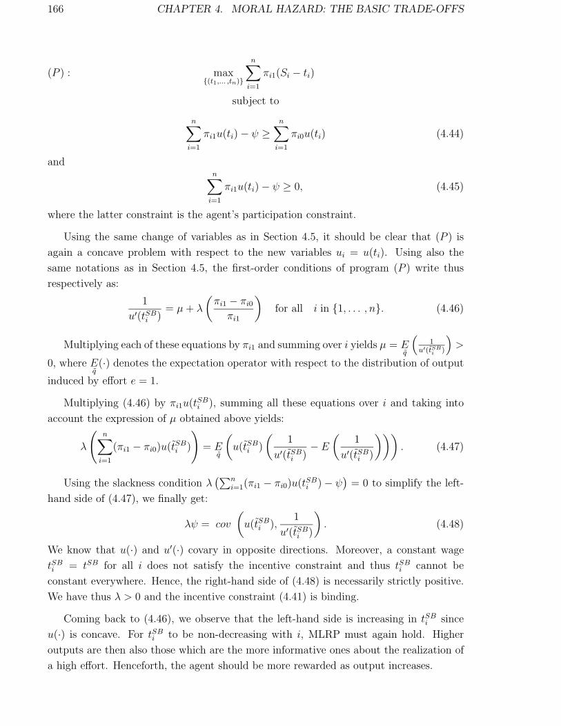
166 CHAPTER 4. MORAL HAZARD: THE BASIC TRADE-OFFS
(P ) : max{(t1,... ,tn)}
n∑i=1
πi1(Si − ti)
subject to
n∑i=1
πi1u(ti)− ψ ≥n∑
i=1
πi0u(ti) (4.44)
andn∑
i=1
πi1u(ti)− ψ ≥ 0, (4.45)
where the latter constraint is the agent’s participation constraint.
Using the same change of variables as in Section 4.5, it should be clear that (P ) is
again a concave problem with respect to the new variables ui = u(ti). Using also the
same notations as in Section 4.5, the first-order conditions of program (P ) write thus
respectively as:
1
u′(tSBi )
= µ + λ
(πi1 − πi0
πi1
)for all i in {1, . . . , n}. (4.46)
Multiplying each of these equations by πi1 and summing over i yields µ = Eq
(1
u′(tSBi )
)>
0, where Eq(·) denotes the expectation operator with respect to the distribution of output
induced by effort e = 1.
Multiplying (4.46) by πi1u(tSBi ), summing all these equations over i and taking into
account the expression of µ obtained above yields:
λ
(n∑
i=1
(πi1 − πi0)u(tSBi )
)= E
q
(u(tSB
i )
(1
u′(tSBi )
− E
(1
u′(tSBi )
))). (4.47)
Using the slackness condition λ(∑n
i=1(πi1 − πi0)u(tSBi )− ψ
)= 0 to simplify the left-
hand side of (4.47), we finally get:
λψ = cov
(u(tSB
i ),1
u′(tSBi )
). (4.48)
We know that u(·) and u′(·) covary in opposite directions. Moreover, a constant wage
tSBi = tSB for all i does not satisfy the incentive constraint and thus tSB
i cannot be
constant everywhere. Hence, the right-hand side of (4.48) is necessarily strictly positive.
We have thus λ > 0 and the incentive constraint (4.41) is binding.
Coming back to (4.46), we observe that the left-hand side is increasing in tSBi since
u(·) is concave. For tSBi to be non-decreasing with i, MLRP must again hold. Higher
outputs are then also those which are the more informative ones about the realization of
a high effort. Henceforth, the agent should be more rewarded as output increases.

4.7. INFORMATIVE SIGNALS TO IMPROVE CONTRACTING 167
4.7 Informative Signals to Improve Contracting
As in the case of adverse selection analyzed in Section 2.15, various verifiable signals can
be used by the principal to improve the provision of incentives to the agent in a moral
hazard framework. These pieces of information can be gathered by different kinds of
information systems which can be internal to the organization or which can be market
information obtained by comparing the agent’s performances with those of other related
agents in the market place. Those practices are known as “benchmarking” or “yardstick
competition”.
4.7.1 Informativeness of Signals
The framework of Section 4.6 with multiple levels of performance is extremely useful
to assess the principal’s benefit from other sources of information than the agent’s sole
performance. To assess the role of improved information structures let us still assume
that there are only two levels of production q and q, and that the principal learns also a
binary signal σ belonging to the set Σ = {σ0, σ1}, which depends directly on the agent’s
effort. More precisely, the following matrix gives the probabilities of each signal σi for i
in {0, 1} as a function of the agent’s effort:
@@
@@
@@
Effort
Signal
e = 0 e = 1
σ1 ν0
1− ν0
ν1
1− ν1σ0
<
>
Note that the signal σ1 (resp. σ0) is “good news” (resp. “bad news”) about the fact
that the agent has exerted a high level of effort. The signal is uninformative on the agent’s
effort when ν0 = ν1.
The signal σ being verifiable, the principal has now the ability to condition the agent’s
performance on four possible different states of nature, yi, for i in {1, . . . , 4}, where each
of these states is defined as follows:

168 CHAPTER 4. MORAL HAZARD: THE BASIC TRADE-OFFS
State of nature Probability Probabilitywhen e0 when e1
y1 = {q, σ1} π0ν0 π1ν1
y2 = {q, σ0} π0(1− ν0) π1(1− ν1)
y3 = {q, σ1} (1− π0)ν0 (1− π1)ν1
y4 = {q, σ0} (1− π0)(1− ν0) (1− π1)(1− ν1)
The signal σ being not related to output, but only to effort, we assume that it does
not affect the principal’s return from the relationship and we have of course S1 = S2 = S
and S3 = S4 = S.12
Denoting by λ and µ the respective multipliers of the agent’s incentive and participa-
tion constraints, the first-order conditions (4.46) become now:
1
u′(tSB1 )
= µ + λ
(π1ν1 − π0ν0
π1ν1
), (4.49)
1
u′(tSB2 )
= µ + λ
(π1(1− ν1)− π0(1− ν0)
π1(1− ν1)
), (4.50)
1
u′(tSB3 )
= µ + λ
((1− π1)ν1 − (1− π0)ν0
(1− π1)ν1
), (4.51)
1
u′(tSB4 )
= µ + λ
((1− π1)(1− ν1)− (1− π0)(1− ν0)
(1− π1)(1− ν1)
). (4.52)
Note that tSB1 = tSB
2 and tSB3 = tSB
4 only when ν1 = ν0, i.e., when σ is not informative
on the agent’s effort. In this case, conditioning the agent’s contribution on an extra risk
σ unrelated to the agent’s effort is of no value for the principal. This can only increase
risk without any incentive benefit. Any compensation t(σ, q) yielding utility u(t(σ, q)) to
the agent can indeed be replaced by a new scheme t(q) which is independent of σ and
such that u(t(q)) = Eσ(u(t(σ, q))) for any q without changing the agent’s incentive and
participation constraints. Furthermore, this new scheme is also less costly to the principal
since Eq(t(q)) < E
(σ,q)t(σ, q). To prove that, note that using the definition of t(q), we have
t(q) = h(Eσ(u(t(σ, q)))
), and thus
Eq(t(q)) = E
q
(h(E
σ(u(t(σ, q))))
)< E
q
(Eσ(h ◦ u(t(σ, q)))
)= E
(σ,q)(t(σ, q)), (4.53)
12In fact, we could allow for some differences in the values of those surpluses in a more general modelwhere the principal’s surplus would write as S(q, σ).

4.7. INFORMATIVE SIGNALS TO IMPROVE CONTRACTING 169
where the first inequality comes from using Jensen’s inequality for h(·) convex, and the
second equality is the Law of Iterated Expectations.
Instead, when σ is informative on the agent’s effort, conditioning the agent’s contri-
bution on the realization of σ has some positive incentive value as shown on equations
(4.49) to (4.52). We state this as a proposition:
Proposition 4.7 : Any signal σ which is informative on the agent’s effort should be used
to condition the agent’s reward.
This result is known as Holmstrom (1979)’s “Sufficient Statistics” Theorem. It
was initially proved in a model wich a continuum of outcomes and a continuum of effort
levels but its logic is the same as above.
4.7.2 More Comparisons among Information Structures
The previous section has shown how the principal can strictly prefer a given information
structure {q, σ} to another structure {q} as soon as the signal σ is informative on the
agent’s effort. More generally, the choice between various information structures will
trade-off the direct cost of these systems, which may increase as the principal uses signals
on the agent’s performance which are more informative, and the possible benefits provided
by these structures in reducing the agency costs.
Let us thus define an information structure π(e) as a n-uple {πi(e)}i∈{1,... ,n} such that
πi(e) ≥ 0 for all i and∑n
i=1 πi(e) = 1. Again, we assume that e can be either 0 or 1 and
to simplify, we denote π(1) = π.
A natural ordering of information systems is provided by Blackwell’s condition stated
below.
Definition 4.3 : The information structure π(e) is sufficient in the sense of Blackwell
for the information structure π(e) if and only there exists a transition matrix13 P =
(pij), (i, j) ∈ {1, . . . , n}2, which is independent of e and which is such that πj(e) =∑ni=1 pjiπi(e), for all e in {0, 1}.
An intuitive example of this ordering is given by the garbling of an information struc-
ture. Then, each signal of information structure 1 is transformed by a purely random
mechanism (independent of the signal considered) into a vector of signals. The new in-
formation, say structure 2, is such that the information structure 1 is sufficient for the
13A transition matrix is such that pij ≥ 0 for all i, and∑n
i=1 pij = 1 for all j.

170 CHAPTER 4. MORAL HAZARD: THE BASIC TRADE-OFFS
information structure 2. The ordering implied by the Blackwell conditions is an inter-
esting expression of dominance since it is a necessary and sufficient condition for any
decision maker to prefer the information structure 1 to information structure 2. We
want to understand whether this natural statistical ordering among information struc-
tures allows us to rank the agency costs in the incentive problems associated with the
information structures π and π.14 To see that, let us define CSB(π) as the second-best
cost of implementing a positive effort when the information structure is π. By definition,
we have CSB(π) =∑n
i=1 πi1tSBi (π) =
∑ni=1 πi1h(uSB
i (π)), where tSBi (π) is given by (4.46).
Note that we make explicit the dependence of these transfers on the information system
since different informations systems may not yield the same second-best transfers and
implementation costs.
We are interested in comparing information structures according to their agency costs.
Let us state first the following definition.
Definition 4.4 : The information structure π is weakly more efficient than the informa-
tion structure π if and only if CSB(π) ≤ CSB(π).
We can then obtain the following comparison:
Proposition 4.8 : If the information structure π is sufficient for the information struc-
ture π in the sense of Blackwell, then π is weakly more efficient than π.
Proof: To prove this result, note first that the definition of the information system π
implies that:
CSB(π) =n∑
i=1
πi1h(uSBi (π)) =
n∑i=1
(n∑
k=1
pikπk1
)h(uSB
i (π)) =n∑
k=1
πk1
(n∑
i=1
pikh(uSBi (π))
)
≥n∑
k=1
πk1h
(n∑
i=1
pikuSBi (π)
), (4.54)
where the second equality uses the definition of π and the last line is obtained from
Jensen’s inequality.
However, uSBi (π) implements a positive effort at a minimal cost when the informa-
tion structure is π so that the agent’s incentive compatibility constraint∑n
i=1(πi1 −πi0)u
SBi (π) = ψ, and his participation constraint
∑ni=1 πi1u
SBi (π) = ψ are both binding.
Using again the definition of π, those two last equations write respectively as:
n∑i=1
(n∑
k=1
pik(πk1 − πk0)
)uSB
i (π) =n∑
k=1
((πk1 − πk0)
(n∑
i=1
pikuSBi (π)
))= ψ (4.55)
14If the principal wants to induce zero effort, he does so by offering a wage which is identically nulwhatever the information system.
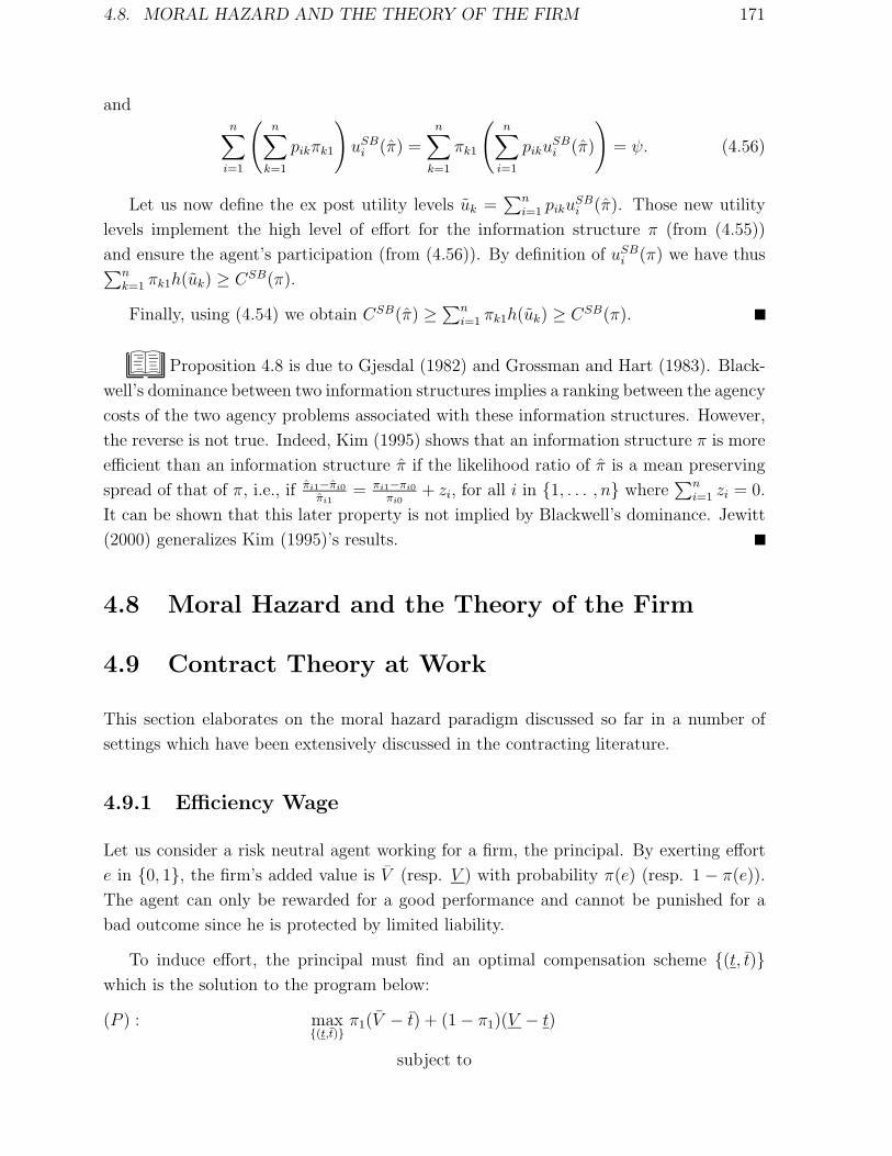
4.8. MORAL HAZARD AND THE THEORY OF THE FIRM 171
andn∑
i=1
(n∑
k=1
pikπk1
)uSB
i (π) =n∑
k=1
πk1
(n∑
i=1
pikuSBi (π)
)= ψ. (4.56)
Let us now define the ex post utility levels uk =∑n
i=1 pikuSBi (π). Those new utility
levels implement the high level of effort for the information structure π (from (4.55))
and ensure the agent’s participation (from (4.56)). By definition of uSBi (π) we have thus∑n
k=1 πk1h(uk) ≥ CSB(π).
Finally, using (4.54) we obtain CSB(π) ≥ ∑ni=1 πk1h(uk) ≥ CSB(π).
Proposition 4.8 is due to Gjesdal (1982) and Grossman and Hart (1983). Black-
well’s dominance between two information structures implies a ranking between the agency
costs of the two agency problems associated with these information structures. However,
the reverse is not true. Indeed, Kim (1995) shows that an information structure π is more
efficient than an information structure π if the likelihood ratio of π is a mean preserving
spread of that of π, i.e., if πi1−πi0
πi1= πi1−πi0
πi0+ zi, for all i in {1, . . . , n} where
∑ni=1 zi = 0.
It can be shown that this later property is not implied by Blackwell’s dominance. Jewitt
(2000) generalizes Kim (1995)’s results.
4.8 Moral Hazard and the Theory of the Firm
4.9 Contract Theory at Work
This section elaborates on the moral hazard paradigm discussed so far in a number of
settings which have been extensively discussed in the contracting literature.
4.9.1 Efficiency Wage
Let us consider a risk neutral agent working for a firm, the principal. By exerting effort
e in {0, 1}, the firm’s added value is V (resp. V ) with probability π(e) (resp. 1 − π(e)).
The agent can only be rewarded for a good performance and cannot be punished for a
bad outcome since he is protected by limited liability.
To induce effort, the principal must find an optimal compensation scheme {(t, t)}which is the solution to the program below:
(P ) : max{(t,t)}
π1(V − t) + (1− π1)(V − t)
subject to

172 CHAPTER 4. MORAL HAZARD: THE BASIC TRADE-OFFS
π1t + (1− π1)t− ψ ≥ π0t + (1− π0)t, (4.57)
π1t + (1− π1)t− ψ ≥ 0, (4.58)
t ≥ 0. (4.59)
The problem is completely isomorphic to that analyzed in Section 4.4. The limited
liability constraint is binding at the optimum and the firm chooses to induce a high effort
when ∆π∆V ≥ π0ψ∆π
. At the optimum, tSB = 0 and tSB > 0. The positive wage tSB = ψ∆π
,
is often called an efficiency wage because it induces the agent to exert a high (efficient)
level of effort. To induce production, the principal must give up to the agent a share of
the firm’s return.
4.9.2 Sharecropping
The moral hazard paradigm has been one of the leading tools used by development
economists to analyze agrarian economies. In the sharecropping example, the princi-
pal is now a landlord and the agent is his tenant. By exerting an effort e in {0, 1}, the
tenant increases (resp. decreases) the probability π(e) (resp. 1 − π(e)) that a large q
(resp. small q) quantity of an agricultural product is produced. The price of this good
is normalized to one so that the principal’s stochastic return of the activity is also q or q
depending on the state of nature.
It is often the case that peasants in developing countries are subject to strong financial
constraints. To model such a setting we assume that the agent is risk neutral and protected
by limited liability. When he wants to induce effort, the principal’s optimal contract must
solve:
(P ) : max{(t,t)}
π1(q − t) + (1− π1)(q − t)
subject to (4.57) to (4.59).
The optimal contract satisfies therefore tSB = 0 and tSB = ψ∆π
. This is again akin to
an efficiency wage. The expected utilities obtained respectively by the principal and the
agent are then given by:
EV SB = π1q + (1− π1)q − π1ψ
∆π, (4.60)
and
EUSB =π0ψ
∆π. (4.61)
The flexible second-best contract described above has sometimes been criticized as
not corresponding to the contractual arrangements observed in most agrarian economies.

4.9. CONTRACT THEORY AT WORK 173
Contracts take often the form of simple linear schedules linking the tenant’s production
to his compensation. Let us now analyze such a simple linear sharing rule between the
landlord and his tenant, with the landlord offering to the agent a fixed share α of the
realized production. Such a sharing rule satisfies automatically the agent’s limited liability
constraint which can therefore be omitted in what follows. Formally, the optimal linear
rule inducing effort must solve:
(P ) : maxα
(1− α)(π1q + (1− π1)q)
subject to
α(π1q + (1− π1)q)− ψ ≥ α(π0q + (1− π0)q), (4.62)
α(π1q + (1− π1)q)− ψ ≥ 0. (4.63)
Obviously, only (4.62) is binding at the optimum and one finds the optimal linear
sharing rule:
αSB =ψ
∆π∆q. (4.64)
Note that αSB < 1 since, for the agricultural activity to be a valuable venture in
the first-best world, we must have ∆π∆q > ψ. Henceforth, the return of the agricultural
activity is shared between the principal and the agent, with high powered incentives (α
close to one) being provided when the disutility of effort ψ is large or when the principal’s
gain from an increase in effort ∆π∆q is small.
This sharing rule yields also the following expected utilities respectively to the principal
and the agent:
EVα = π1q + (1− π1)q −(
π1q + (1− π1)q
∆q
)ψ
∆π, (4.65)
and
EUα =
(π0q + (1− π0)q
∆q
)ψ
∆π. (4.66)
Comparing respectively (4.60) and (4.65) on the one hand and (4.61) and (4.66) on
the other hand, we observe that the constant sharing rule benefits the agent but not the
principal. A linear contract is less powerful than the optimal second-best contract since
the former is an inefficient way to extract rent from the agent even if it still provides
sufficient incentives to exert effort. Indeed, with a linear sharing rule, the agent always
benefits from a positive return on his production even in the worst state of nature. This

174 CHAPTER 4. MORAL HAZARD: THE BASIC TRADE-OFFS
positive return yields to the agent more than what is requested by the optimal second-
best contract in the worst state of nature, namely zero. Punishing the agent for a bad
performance is thus found to be rather difficult with a linear rule.
A linear sharing rule allows the agent to keep some strictly positive information rent
EUα. If the space of available contracts is extended to allow for fixed fees β, the principal
can nevertheless bring down the agent to the level of his outside opportunity by setting a
fixed fee βSB equal to(
π0q+(1−π0)q
∆q
)ψ
∆π.
4.9.3 Wholesale Contracts
Let us now consider a manufacturer-retailer relationship. The manufacturer supplies at
constant marginal cost c an intermediate good to the risk averse retailer who sells this
good on a final market. Demand on this market is high (resp. low) D(p) (resp. D(p))
with probability π(e) where, again, e is in {0, 1} and p denotes the price for the final
good. Effort e is exerted by the retailer who can increase the probability that demand
is high if after-sales services are efficiently performed. The wholesale contract consists of
a retail price maintenance agreement specifying the prices p and p on the final market
with a sharing of the profits, namely {(t, p); (t, p)}. When he wants to induce effort, the
optimal contract offered by the manufacturer solves therefore the following problem:
(P ) : max{(t,p);(t,p)}
π1((p− c)D(p)− t) + (1− π1)((p− c)D(p)− t)
subject to (4.3) and (4.4).
The solution to this problem is obtained by appending to the transfers given in (4.32)
and (4.33) the following expressions of the retail prices p∗+ D(p∗)D′(p∗) = c, and p∗+
D(p∗)D′(p∗) = c.
4.9.4 Financial Contracts
Moral hazard is a quite important issue in financial markets. Let us now assume that
a risk averse entrepreneur wants to start a project which requires an initial investment
worth an amount I. The entrepreneur has no cash of his own and must raise money from
a bank or any other financial intermediary. The return on the project is random and
equal to π (resp. π) with probability π(e) (resp. 1−π(e)) where the effort exerted by the
entrepreneur e belongs to {0, 1}. We denote by ∆V = V − V > 0 the spread of profits.
The financial contract consists of repayments {(z, z)} depending on whether the project
is successful or not.
To induce effort from the borrower, the risk neutral lender’s program writes as:

4.9. CONTRACT THEORY AT WORK 175
(P ) : max{(t,t)}
(π1z + (1− π1)z − I)
subject to
π1u(V − z) + (1− π1)u(V − z)− ψ ≥ π0u(V − z) + (1− π0)u(V − z), (4.67)
π1u(V − z) + (1− π1)u(V − z)− ψ ≥ 0, (4.68)
where (4.67) and (4.68) are respectively the agent’s incentive and participation constraints.
Note that the project is a valuable venture if it provides to the bank a positive expected
profit.
With the change of variables, t = V − z and t = V − z, the principal’s program takes
its usual form. This change of variables also highlights that everything happens as if the
lender was benefitting himself directly from the return of the project paying then to the
agent only a fraction of the returns in these different states of nature.
Let us define the second-best cost of implementing a positive effort CSB as in Section
4.5 and let us assume that ∆π∆V ≥ CSB, so that the lender wants to induce a positive
effort level even in a second best environment. The lender’s expected profit is worth:
V1 = π1V + (1− π1)V − CSB − I. (4.69)
Let us now parameterize projects according to the size of the investment I. Only the
projects with positive value V1 > 0 will be financed. This requires that investment is low
enough and, typically, we must have:
I < ISB = π1V + (1− π1)V − CSB. (4.70)
Under complete information and no moral hazard, the project would instead be fi-
nanced as soon as
I < I∗ = π1V + (1− π1)V . (4.71)
For intermediary values of the investment, i.e., for I in [ISB, I∗], moral hazard implies
that some projects are financed under complete information, but no longer under moral
hazard. This is akin to some form of credit rationing.
Finally, note that the optimal financial contract offered to the risk averse and cashless
entrepreneur does not satisfy the limited liability constraint t ≥ 0. Indeed, we have
tSB = h(ψ − π1∆ψ
∆π
)< 0. To induce effort, the agent must bear some risk which implies
a negative payoff in the bad state of nature. Adding the limited liability constraint,

176 CHAPTER 4. MORAL HAZARD: THE BASIC TRADE-OFFS
the optimal contract would instead entail tLL = 0 and tLL = h(
ψ∆π
). Interestingly, this
contract has sometimes been interpreted in the finance literature as a debt contract, with
no money being left to the borrower in the bad state of nature and the residual being
pocketed by the lender in the good state of nature.
Finally, note that:
tLL − tLL = h
(ψ
∆π
)< tSB − tSB = h
(ψ + (1− π)
ψ
∆π
)− h
(ψ − πψ
∆π
), (4.72)
since h(·) is strictly convex and h(0) = 0. This inequality shows that the debt contract
has less incentive power than the optimal incentive contract. Indeed, it becomes harder
to spread the agent’s payments between both states of nature to induce effort if the agent
is protected by limited liability. The agent being interested only by his payoff in the high
state of nature, only rewards are attractive.
Remark: The finance literature starting with Jensen and Meckling (1976) has stressed
that moral hazard within the firm may not be due to the desire of the manager to avoid
costly effort but, instead, to his desire of choosing projects with private benefits. Those
private benefits arise, for instance, when the manager devotes the resources of the firm to
consume perquisities.
The modeling of these private benefits is very similar to that of the standard moral
hazard problem viewed so far.15 Let us consider that the risk-neutral manager can choose
between a “good” and a “bad” project. The shareholders’ return of the good project is V
with probability π1 and 0 otherwise. However, by choosing the bad project, the manager
gets a private benefit B which is strictly positive. A contract is again a pair of transfers
{(t, t)} where, assuming limited liability, t = 0.
The manager chooses the good project when the following incentive constraint is sat-
isfied:
π1t ≥ π0t + B, (4.73)
which amounts to:
t ≥ B
∆π. (4.74)
This constraint being obviously binding at the optimum of the financier’s problem,
the latter gets an expected payoff V1 such that:
V1 = π1
(V − B
∆π
)− I (4.75)
15The private benefit is an output which is not observed by the principal, while effort was an unobservedinput.

4.9. CONTRACT THEORY AT WORK 177
where I is the investment cost that financiers have incurred. Obviously, compared with
complete information, the set of valuable investments is reduced under moral hazard
because of the agency cost incurred to avoid private benefits.
4.9.5 Insurance Contract
Moral hazard also undermines the functioning of insurance markets. We consider now a
risk averse agent with utility function u(·) and initial wealth w. With probability π(e)
(resp. 1− π(e)) the agent has no (resp. an) accident and pays an amount z (resp. z) to
an insurance company. The damage incurred by the agent is worth d. Effort e in {0, 1}can now be interpreted as a level of safety care.
Monopoly: To make things simpler, and as in Section 2.16.6, the insurance company
is first assumed to be a monopoly and has all the bargaining power when offering the
insurance contract to the insuree. To induce effort from the insuree, the optimal insurance
contract must solve:
(P ) : max{(z,z)}
π1z + (1− π1)z
subject to
π1u(w − z) + (1− π1)u(w − d− z)− ψ ≥ π0u(w − z) + (1− π0)u(w − d− z), (4.76)
π1u(w − z) + (1− π1)u(w − d− z)− ψ ≥ u(w), (4.77)
where w is the certainty equivalent of the agent’s wealth when he does not subscribe any
insurance and exerts no effort. w is implicitly defined as u(w) = π1u(w) + (1− π1)u(w−d)− ψ.16
Note that the right-hand side of (4.77) is not zero. Except for this non zero reservation
value, the problem is very close to that of Section 4.5 after having replaced variables so
that the net transfers received by the agent are t = w − z and t = w − d− z and noticed
that S = w and S = w −D.
Both constraints (4.76) and (4.77) are again binding at the optimum and the second-
best cost of inducing effort writes now as:
CSB(w) = π1h
(ψ + u(w) + (1− π1)
ψ
∆π
)+ (1− π1)h
(ψ + u(w)− π1ψ
∆π
). (4.78)
16We assume that the agent wants to exert an effort in the absence of an insurance contract, i.e.u(w) − u(w − d) > ψ
∆π . One could assume instead that he does not want to exert effort when he is notinsured. Then, his status quo utility level is π0u(w) + (1− π0)u(w − d) = u(w′).

178 CHAPTER 4. MORAL HAZARD: THE BASIC TRADE-OFFS
Without moral hazard this cost of inducing effort would instead be:
CFB(w) = h(ψ + u(w)). (4.79)
Let us thus denote by AC(w) = CSB(w) − CFB(w), the agency cost incurred by the
principal, i.e., the difference between the second-best and the first-best cost of inducing
effort. This difference is the agency cost from moral hazard. Differentiating with respect
to w, we have:
AC ′(w) = u′(w)
(π1h
′ (ψ + u(w) + (1− π1)ψ
∆π
)+ (1− π1)h
′ (ψ + u(w)− π1ψ∆π
)−h′(ψ + u(w))
)> 0, (4.80)
if h′(·) is convex. In fact, we let the reader check that this latter concavity is insured when
pu(x) < 3ru(x) where pu(x) = −u′′′(x)u′′(x)
is the agent’s degree of prudence and ru(x) = −u′′(x)u′(x)
is his degree of risk aversion.17
The fact that AC(·) is monotonically increasing with w can be interpreted as saying
that, as the agent’s wealth increases, there is more distortion due to moral hazard in the
decision of the insurance company to induce effort or not. However, the sufficient condition
on h(·) needed to obtain this result is somewhat intricate. This highlights the important
difficulties that modelers often face when they want to derive simple comparative statics
results from even a simple agency problem.
Competitive Market: The insurance market is often viewed as an archetypical ex-
ample of a perfectly competitive market where insurers’ profits are driven to zero. Without
entering too much into the difficult issues of competitive markets plagued by agency prob-
lems, it is nevertheless useful to characterize the equilibrium contract inducing a positive
effort. Because of perfect competition among insurance companies, this contract should
maximize the agent’s expected utility subject to the standard incentive compatibility
constraint (written with our usual change of variables)
u− u ≥ ψ
∆π, (4.81)
and the non zero-profit constraint of the insurance company:
π1(w − h(u)) + (1− π1)(w − d− h(u)) ≥ 0. (4.82)
The equilibrium contract must therefore solve the following problem:
(P ) : max{(u,u)}
π1u + (1− π1)u− ψ
subject to (4.81) and (4.82).17This latter property holds when u(·) is CARA. See also Wambach (2000) for such comparative statics.

4.9. CONTRACT THEORY AT WORK 179
Denoting by λ and µ the respective multiplier of those two constraints, the necessary
and sufficient Kuhn and Tucker conditions for this concave problem write respectively as:
π1 + λ = µπ1h′(uM), (4.83)
and
1− π1 − λ = µ(1− π1)h′(uM). (4.84)
Summing those two equations immediately yields that:
µ =1
π1h′(uM) + (1− π1)h′(uM)> 0. (4.85)
Henceforth, the zero profit constraint is automatically satisfied by this equilibrium
contract. Similarly, we also find that:
λ = π1(1− π1)(h′(uM)− h′(uM))
π1h′(uM) + (1− π1)h′(uM)> 0, (4.86)
since h(·) is convex and uM > uM is necessary to guarantee that (4.81) holds. The
incentive compatibility constraint is also binding at the equilibrium contract.
Denoting by UM the agent’s expected utility when exerting a positive effort, the
binding insurer’s zero profit constraint can thus be rewritten as:
π1h
(UM + ψ + (1− π1)
ψ
∆π
)+ (1− π1)h
(UM + ψ − π1
ψ
∆π
)= w − d(1− π1). (4.87)
The market does not break down as long as (4.87) defines implicitly a value UM which
is greater than what the agent gets by not taking any insurance contract. Let denote by
U this utility level:
U = maxe∈{0,1}
π(e)u(w) + (1− π(e))u(w −D)− ψ(e).
Note that, under complete information, the agent would be perfectly insured and would
exert a positive effort. He would then get a positive expected utility U∗ such that h(U∗+
ψ) = w − d(1− π1). Again, the market does not breakdown as long as U∗ > U .
Let us take a case where U∗ is greater than U under complete information, i.e., inducing
effort has a positive social value w− d(1− π1)− h(ψ) > 0. Then, this condition certainly
does not guarantee that UM defined implicitly by (4.87) remains greater than U . Indeed,
from Jensen’s inequality and h(·) convex, the left-hand side of (4.87) is strictly greater
than h(UM+ψ). Moral hazard may then imply an inefficiency of the competitive insurance
market, in the sense that it cannot induce a positive effort level.

180 CHAPTER 4. MORAL HAZARD: THE BASIC TRADE-OFFS
4.10 Commitment under Moral Hazard
The assumption of full commitment to an incentive scheme was already discussed in
Section 2.11 in the case of adverse selection. This issue is also quite important under
moral hazard. Indeed to induce a positive effort level, the principal must let the risk
averse agent bear some risk. However, once this effort is sunk and before uncertainty is
resolved, the principal would like to offer more insurance to the agent to avoid paying an
excessive agency cost. For this reinsurance stage to have any impact, the principal must
be aware, maybe through a direct observation of the effort itself, or by indirectly getting
a signal correlated with this effort, that effort has already been performed. Of course,
the renegotiation stage would be perfectly anticipated by the rational agent at the time
of exerting effort. Renegotiation is then unlikely to lead to complete insurance ex post,
since the agent would then have no incentive to exert effort in the first place.18 We will
discuss the issues of moral hazard and renegotiation more fully in Volume III.
18See Fudenberg and Tirole (1990).
4.10. COMMITMENT UNDER MORAL HAZARD 181
APPENDIX 4.1: Proof of Proposition 4.2
• Suppose first that 0 ≤ ` ≤ π0
∆πψ. We conjecture that (4.15) and (4.16) are the only
relevant constraints. Of course, since the principal is willing to minimize the payments
made to the agent, both constraints must be binding. Hence, tSB = −` and tSB = −`+ ψ∆π
.
We check that (4.17) is satisfied since −`+ ψ∆π
> −`. We check also that (4.16) is strictly
satisfied since π1tSB + (1− π1)t
SB − ψ = −` + π0
∆πψ > 0.
• For ` > − π0
∆πψ, note that the transfers t∗ = − π0
∆πψ and t∗ = −ψ + (1−π1)
∆πψ > t∗ are
such that both constraints (4.17) and (4.18) are strictly satisfied and such that (4.15) is
binding.
APPENDIX 4.2: A Continuum of Performances
Let us now assume that the level of performance q is drawn from a continuous dis-
tribution with a cumulative function F (·|e) on the support [q, q]. This distribution is
conditional on the agent’s level of effort which still takes two possible values e in {0, 1}.We denote by f(·|e) the density corresponding to the above distributions. A contract t(q)
inducing a positive effort in this context must satisfy the incentive constraint∫ q
q
u(t(q))f(q|1)dq − ψ ≥∫ q
q
u(t(q))f(q|0)dq, (4.88)
and the participation constraint∫ q
q
u(t(q))f(q|1)dq − ψ ≥ 0. (4.89)
The risk neutral principal’s problem writes thus as:
(P ) : max{t(q)}
∫ q
q
(S(q)− t(q))f(q|1)dq,
subject to (4.88) and (4.89).
Denoting by λ and µ the respective multipliers of (4.88) and (4.89), the Lagrangean of
(P ) writes as L(q, t) = (S(q)− t)f(q|1)+λ(u(t)(f(q|1)−f(q|0))−ψ)+µ(u(t)f(q|1)−ψ).
Optimizing pointwise with respect to t yields:
1
u′(tSB(q))= µ + λ
(f(q|1)− f(q|0)
f(q|1)
). (4.90)

182 CHAPTER 4. MORAL HAZARD: THE BASIC TRADE-OFFS
Multiplying (4.90) by f1(q) and taking expectations,19 we obtain as in the main text:
µ = E
(1
u′(tSB(q))
)> 0, (4.91)
where Eq(·) is the expectation operator with respect to the probability distribution of
output induced by an effort eSB. Finally, using this expression of µ, inserting into (4.90)
and multiplying by f(q|1)u(tSB(q)), we obtain:
λ(f(q|1)− f(q|0))u(tSB(q)) = f(q|1)u(tSB(q))
(1
u′(tSB(q))− E
(1
u′(tSB(q))
)). (4.92)
Integrating over [q, q] and taking into account that λ(∫ q
q(f(q|1)− f(q|0))u(tSB(q))dq − ψ
)=
0 yields λψ = cov(u(tSB(q)), 1
u′(tSB(q))
)> 0.
Hence, λ ≥ 0 since u(·) and u′(·) vary in opposite directions. λ = 0 only if tSB(q)
is a constant but, then, the incentive constraint is necessarily violated. Hence, we have
necessarily λ > 0. Finally, tSB(π) is monotonically increasing in π when the monotone
likelihood property ddq
(f(q|1)−f(q|0)
f(q|1)
)> 0 is satisfied.
APPENDIX 4.3: Proof of Proposition 4.6
Indeed, let J be the set of indices j such thatπj1−πj0
πj1= maxi
{πi1−πi0
πi1
}. If J = {n},
then we have tn = ψπn1−πn0
and ti = 0 for i < n. Otherwise ti = 0 if i 6∈ J and for i ∈ J ,
the transfer ti must satisfy the incentive constraint as an equality.∑
i∈J(πi1− πi0)ti = ψ,
and the principal (and the agent) are indifferent to the profiles of positive transfers. They
can be chosen positive and increasing for example.
19Note that∫ q
qf(q|e)dq = 1 for e in {0, 1}.

Chapter 5
Incentive and ParticipationContraints with Moral Hazard
5.1 Introduction
In Chapter 4, we have already stressed the various conflicts which may appear in a moral
hazard environment. The analysis of these conflicts, either under limited liability or risk
aversion, was made easy because of our focus on a simple 2 by 2 environment with a binary
effort and two levels of performance. The simple interaction between a single incentive
constraint with either a limited liability constraint or a participation constraint was then
quite straightforward.
However, moral hazard models inherit also the major difficulties of Incentive Theory
already present in our investigation of complex adverse selection models made in Chapter
3. Indeed, when one moves away from the 2 by 2 (by far too simplistic) model of Chapter
4, numerous incentive constraints have also to be taken into account in complex moral
hazard environments. The analysis becomes much harder and characterizing the optimal
incentive contracts is a difficult task. Examples of such complex contracting environments
abound. Effort may no longer be binary but, instead, may be better characterized as a
continuous variable. A manager may no longer choose between working or not on a
project but may be able to fine tune the exact spend on this project. Even worse, the
agent’s actions may no longer be summarized by a one-dimensional parameter but may be
better described by a whole array of control variables which are technologically linked. For
instance, the manager of a firm has to choose how to allocate his effort between productive
activities and monitoring his peers or other workers. The manager’s performances, i.e., his
profit, may also be better approximated as a continuous variable, a less crude assumption
than that made in Chapter 4.1 Real world incentive schemes for the manager of the firm
1Appendix 4.1 already gives an example of such an analysis with a continuum of performances and
183

184 CHAPTER 5. INCENTIVE AND PARTICIPATION CONTRAINTS
are not based on a discrete number of performances but on the more continuous level of
profit of the firm. Lastly, the agent’s preferences over effort and consumption may no
longer be separable as we have assumed in Chapter 4.
Mirroring as much as possible the analysis made in Chapter 3 for the case of adverse
selection, we argue here that complex contractual environments with moral hazard raise
also many new difficulties for the characterization of the binding incentive and participa-
tion constraints. Again mimicking what was done in Chapter 3, we propose a classification
of the new contractual settings analyzed in the present chapter. Each of those categories
corresponds to a particular perturbation of the standard moral hazard trade-offs analyzed
in Chapter 2.
• Models with a hardening of the agent’s incentive constraints: Let us consider a first class
of models where the agent can exert more than two possible levels of effort. The agent may
choose his one-dimensional action within a finite set or may be able to fine tune continously
his effort supply. In both cases, the agent’s performance remains nevertheless a single
dimensional vector. Alternatively, the agent may be performing several tasks on the
principal’s behalf, controlling thus various dimensions of effort with each of those efforts
affecting a particular aspect of the agent’s performance. In those complex contracting
environments, a major difficulty is to ensure that local incentive constraints, which are
the easiest ones to handle, still drive the design of incentives.
When the agent’s performance has a single dimension, we first derive the second-best
cost of implementing any given level of effort. This cost is obtained by minimizing the
agent’s expected payment subject to his incentive and participation constraints. As in
Chapter 4, it is generally true that the second-best cost is greater than the first-best
cost as soon as one incentive contraint is binding. Second, we generalize the second-best
analysis of Chapter 4 to find the optimal effort level that the principal wants to induce
under moral hazard. This analysis already shows that there is no general lessons on the
nature of the distortion entailed by moral hazard. The second-best level of effort may
be either higher or lower than its first-best value, contrary to our findings in the binary
effort model of Chapter 4. We then develop the so-called “first-order approach” to moral
hazard problems where effort is a continuous variable. This approach replaces the set of
possible incentive constraints by a local incentive constraint, a legitimate step provided
that the agent’s problem is concave. This concavity is, in turn, obtained under rather
stringent assumptions, namely the cumulative distribution function of the performance
level should be a convex function of the agent’s effort (CCFD) and the monotone likeli-
hood property (MLRP ) should also be satisfied. As we have already seen in Chapter 4,
this latter property also implies that the agent’s compensation schedule is increasing with
two levels of effort.

5.1. INTRODUCTION 185
this performance.
In practice, the agent’s effort is often better characterized as a multi-dimensional
variable. For instance, a retailer selling goods on the manufacturer’s behalf must reduce
retailing costs but also improve after-sales services. A worker is not only involved in
productive tasks but must sometimes be also involved in monitoring his peers. A tenant
must simultaneously choose the quality of the crops he seeds and the level of physical
investment he should make. A teacher must allocate his time between doing research
and supervising students. All these examples belong to the class of multi-task incentive
problems. In those models, agency costs are significantly affected by the possible conflicts
in incentivizing the various tasks performed by the agent. The characterization of the
optimal contract depends on the complementarity or substitutability of the tasks. The
technological relationship between tasks has thus strong incentive consequences. Viewing
the relationship between the principal and his agent as a cluster of various transactions
significantly extends standard theory. New issues arise in such a framework. For instance,
one can study how the distribution of efforts along those different dimensions of the agent’s
activity or the degrees of informativeness of the different performances affect the power
of incentives, deriving from such analysis rich lessons for organizational design.
Even though the relevant literature2 has been mostly developed in a particular frame-
work,3 we have found useful to recast the lessons of this literature in a discrete framework
which extends quite naturally the standard model of Chapter 4. Doing so, we clearly
gain in consistency by offering an integrated framework all over the book. Moreover,
this discrete modeling allows us to discuss the conditions under which non-local incentive
constraints affect the design of incentives, giving us strong economic intuitions about the
economic phenomenon at stakes in this multi-task environment. Keeping this framework,
we also present a number of important examples of the multi-task principal-agent models.
These applications cover a broad range of issues like the interlinking of agrarian contracts,
the design of incentive schemes based on aggregate performances, and finally the choice of
vertically integrating or not a downstream unit and its consequences for the comparison
between the power of incentives in market environments and within firms.
• Models with a hardening of the agent’s participation constraint: One peculiarity of the
principal-agent models presented so far is that, even though various incentive constraints
might be taken into account by the principal, the separability of the agent’s utility function
between consumption and effort implies that giving up an ex ante rent to the agent is
never optimal from the principal’s point of view. Instead, with a non-separability between
2See Holmstrom and Milgrom (1991) and (1994).3This framework considers the case of a continuum of possible performances, a continuum of possible
effort levels on each task and a disutility of effort being evaluated in monetary terms with CARA utilityfunctions.

186 CHAPTER 5. INCENTIVE AND PARTICIPATION CONTRAINTS
consumption and effort in the agent’s utility function, the conflict between incentive and
participation constraints may be better solved by leaving a positive ex ante rent to the
agent. Leaving such a rent allows the principal to benefit from wealth effects which may
reduce the cost of providing incentives.
• Models with constraints on transfers: Finally, we also replace the conflict between incen-
tive and participation constraints by the conflict between incentive and budget balance
constraints which appears in the optimal taxation literature. Again, in a model with a
binary level of effort, under-provision of effort appears with moral hazard.
Section 5.2 presents the straightforward extensions of the standard model of Chapter
4 to the cases where the agent can perform more than two and possibly a continuum of
levels of effort. We discuss there the two-step characterization of the second-best optimum
with, first, the derivation of the second-best cost of implementing a level of effort, and
second the analysis of the trade-off between the benefit and the cost of implementing
any given effort. We prove, by exhibiting an example, that the second-best level of effort
in an insurance-efficiency trade-off can be upwards distorted. This shows therefore that
complex moral hazard models may fail to perpetuate the simple lessons of Chapter 4.
Nevertheless, we also provide a limited liability rent-efficiency trade-off with a continuum
of levels of effort where the basic lessons of Section 4.6.1 carry over. The trade-off between
the extraction of the limited liability rent and allocative efficiency always calls for a
reduction in the expected volume of trade. Finally, this section ends with an exposition
of the “first-order approach” and the many technical problems it raises. When it applies,
the “first-order approach” allows the modeler to replace the infinitely many incentive
constraints arising when the agent controls a continuous effort variable by a simple first-
order condition. Section 5.3 deals with a multi-task model, solving first for the optimal
contracts inducing efforts on both dimensions of the agent’s activity and then deriving the
second-best level of effort on each of these dimensions. This analysis is first performed in
the simple framework of a risk neutral agent who is protected by limited liability. Then, we
turn to the somewhat more complex case of risk aversion. We show the possible origins
of diseconomies of scope in agency costs and we discuss their precise origins. Several
examples of multi-task agency models are then presented. Section 5.4 analyzes the case
where the agent’s utility function is no longer separable between consumption and effort.
We discuss there the conditions under which the agent’s participation constraint may
not be binding at the optimum. We also provide in that section a simple example of
preferences where the disutility of effort can be expressed in monetary terms. Despite the
non-separability between effort and consumption, the optimal contract keeps almost the
same features as in the case of separability.4 Finally, Section 5.5 analyzes the trade-off
4This example will be useful later on in Chapter 9, when we will investigate how optimal contratsmay be linear in moral hazard environments.
5.2. MORE THAN TWO LEVELS OF EFFORT 187
between efficiency and redistribution in a moral hazard context.
5.2 More Than Two Levels of Effort
5.2.1 A Discrete Model
Let us first extend the basic model of Chapter 4 by now allowing more than two levels
of effort. Consider the more general case with n levels of production q1 < q2 < . . . < qn
and K levels of effort with 0 = e0 < e1 < . . . < eK−1 and the following disutilities of
effort ψ(ek) = ψk for all k in {0, . . . , K− 1}. We still make the normalization ψ0 = 0 and
assume that ψk is increasing in k. Let πik for i in {1, . . . , n} also denote the probability
of production qi when the effort level is ek. The agent has still a separable utility function
over monetary transfer and effort U = u(t) − ψ(e) where u(·) is increasing and concave
(u′(·) > 0 and u′′(·) ≤ 0). In such an environment, a contract is a set of transfers {t1, ...tn}corresponding to each possible output levels.
As usual, we proceed in two steps. First, we compute the second-best cost of inducing
effort ek for the principal. We denote this cost by CSBk . Second, we find the optimal level
of effort from the principal’s point of view, taking into account both the costs and benefits
of each action ek.
Let us thus define (Pk) the cost minimization problem of a principal willing to imple-
ment effort ek. Using our, by now standard, change of variables, the important variables
are the utility levels in each state of nature, i.e., ui = u(ti) or alternatively ti = h(ui)
where h = u−1. (Pk) is a concave problem which writes as:
(Pk) : min{(u1,... ,un)}
n∑i=1
πikh(ui)
subject to
n∑i=1
(πik − πik′)ui ≥ ψk − ψk′ for all k′ 6= k, (5.1)
n∑i=1
πikui − ψk ≥ 0. (5.2)
(5.1) is the incentive constraint preventing the agent from exerting effort ek′ , for k′ 6= k,
when the principal wants to implement effort ek. There are K − 1 such constraints. (5.2)
is the agent’s participation constraint when he exerts effort ek. We denote by λk′k the

188 CHAPTER 5. INCENTIVE AND PARTICIPATION CONTRAINTS
multiplier of (5.1) and still, as in Chapter 4, by µ the multiplier of (5.2). The value of
this problem is the second-best cost of implementation CSBk for effort ek.
It should be immediately clear that the second-best cost of implementing effort ek is
such that CSBk ≥ CFB
k = h(ψk), where CFBk denotes the first-best cost of implementing
effort ek. This is so because the presence of incentive constraints in problem (Pk) implies
that the value of this problem is necessarily not greater than under complete information.
Note that the inequality above is strict whenever one of the incentive constraints (5.1) is
binding at the optimum of (Pk).
The necessary and sufficient first-order conditions for the optimization of program (Pk)
write thus as:
1
u′(tik)= µ +
∑k′ 6=k
λk′k
(πik − πik′
πik
), i = 1, . . . , n, (5.3)
where tik is the transfer given to the agent in state i when the principal wants to implement
effort ek.
The new difficulty coming with more than two levels of effort is that there may be
several incentive constraints binding, i.e., several multipliers λk′k which may be different
from zero. Looking only at local incentive constraints may not be enough to characterize
the solution to (Pk) and the optimal payments are then the solutions of a complex system
of nonlinear equations. However, if the only binding incentive constraint is the local
downward incentive constraint, the first-order condition for problem (Pk) writes simply
as:
1
u′(tik)= µ + λk−1
k
(πik − πi(k−1)
πik
). (5.4)
When the cumulative distribution function of production is a convex function of the
level of effort, and when the monotone likelihood ratio assumption holds, the local ap-
proach described above can be validated as it has been shown by Grossman and Hart
(1983). We prove this proposition in Section 5.2.3. for the case of a continuum of effort
levels and a continuum of performances.
Even if describing the behavior of the second-best cost of implementation CSBk is in
general a difficult task, one may try to already get some insights on how the principal
chooses the second-best level of effort. The optimal second-best effort is indeed defined
as eSB = arg maxek
∑ni=1 πikSi − CSB
k .5
Finding this second-best effort eSB is a rather difficult problem and there is, a priori,
no reason to be sure that it is below its first-best value. Under- as well as over-provision
of effort may be obtained at the second-best.5If there are several such maximizers, just pick any of them.

5.2. MORE THAN TWO LEVELS OF EFFORT 189
Under-provision was already obtained in Chapter 4. To see that over-provision may
also arise, let us consider the following example with three possible levels of effort e0, e1
and e2, and two possible outcomes yielding respectively S and S to the principal. The
probabilities that S realizes are respectively π0, π1 and π2 with π0 < π1 < π2 and the
corresponding disutilities of effort are ψ0 = 0 < ψ1 < ψ2. Under complete information,
the intermediate effort is chosen when:
h(ψ1)
π1 − π0
< S − S <h(ψ2)− h(ψ1)
π2 − π1
. (5.5)
The first inequality means that effort e1 is preferred to e0. The second inequality
means that e1 is also preferred to e2.
Under moral hazard, let us first observe that the first-best effort e1 may no longer be
implementable. Indeed, let denote by u and u the levels of utility offered to the agent
when S and S realize. Incentive compatibility requires that:
u− u ≥ ψ1
π1 − π0
(5.6)
so that the agent prefers exerting effort e1 rather than e0. Similarly, we must also have
u− u ≤ ψ2 − ψ1
π2 − π1
(5.7)
to insure that the agent prefers exerting effort e1 than e2. However, when ψ2−ψ1
π2−π1< ψ1
π1−π0,
the set of payoffs (u, u) such that (5.6) and (5.7) are both satisfied is empty. Hence, e1
can no longer be implemented.
Effort e0 remains obviously implementable with a null payment in each state of nature.
Finally, effort e2 is implementable when the incentive constraint
u− u ≥ max
{ψ2 − ψ1
π2 − π1
;ψ2
π2 − π0
}(5.8)
which ensures that effort e2 is preferred to both e1 and e0, and the participation constraint
π2u + (1− π2)u− ψ2 ≥ 0, (5.9)
are both satisfied.
When ψ2−ψ1
π2−π1< ψ2
π2−π0, the maximand on the right-hand side of (5.8) is ψ2
π2−π0. Hence,
the second-best cost of implementing effort e2 can be easily computed as:
CSB2 = π2h
(ψ2 +
(1− π2)ψ2
π2 − π0
)+ (1− π2)h
(ψ2 − π2ψ2
π2 − π0
). (5.10)

190 CHAPTER 5. INCENTIVE AND PARTICIPATION CONTRAINTS
Therefore, effort e2 is second-best optimal when
S − S >CSB
2
π2 − π0
. (5.11)
It is easy to check that one can find values of S−S so that (5.5) and (5.11) both hold
simultaneously. We conclude from that:
Proposition 5.1 : With more than two levels of effort, the second-best effort level may
be greater than the first-best level.
5.2.2 Two Outcomes with a Continuum of Effort Levels
To reduce the cumbersome difficulty of the discrete case, modelers have often preferred to
allow for a continuum of effort levels. With more than two states of nature, one meets soon
important technical problems analyzed in Section 5.2.3 below. With only two possible
levels of performance, the analysis remains nevertheless quite tractable as we see in this
section.
To make some progress in this direction, we reparametrize the model by assuming
that π(e) = e, for all e in [0, 1]. Henceforth, the agent’s effort level equals the probability
of a high performance. The disutility of effort function ψ(e) is increasing and convex in
e (ψ′ > 0 and ψ′′ ≥ 0). Moreover, to insure always interior solutions, we assume that
the Inada conditions ψ′(0) = 0 and ψ′(1) = +∞ both hold. Let us finally consider a risk
neutral agent with zero initial wealth who is protected by limited liability constraints:
t ≥ 0 (5.12)
and
t ≥ 0. (5.13)
Faced with an incentive contract {(t, t)}, this agent chooses an effort e such that
e = arg maxe∈[0,1]
et + (1− e)t− ψ(e). (5.14)
By strict concavity of the agent’s objective function, the incentive constraint rewrites
with the following necessary and sufficient first-order condition:
t− t = ψ′(e). (5.15)
The principal’s program writes now as:

5.2. MORE THAN TWO LEVELS OF EFFORT 191
(P ) : max{(e,t,t)}
eS + (1− e)S − et− (1− e)t
subject to (5.12), (5.13) and (5.15).
As in the model of Section 4.3, the limited liability constraint (5.12) (resp. (5.13)) is
again binding (resp. slack). Replacing t by ψ′(e) into the principal’s objective function,
the principal’s reduced program (P ′) writes thus as:
(P ′) : maxe∈[0,1]
eS + (1− e)S − eψ′(e).
When ψ′′′(·) > 0, the principal’s objective function is strictly concave in e and direct
optimization leads to the following expression for the second-best level of effort eSB:
∆S = ψ′(eSB) + eSBψ′′(eSB). (5.16)
This second-best effort is obviously lower than the first-best effort e∗ which is defined
by
∆S = ψ′(e∗). (5.17)
The first-best effort is such that the marginal benefit ∆S of increasing effort by a
small amount de is just equal to the marginal disutility of doing so ψ′(e∗)de. Under
moral hazard, the marginal benefit ∆Sde must equal the marginal cost ψ′(eSB)de plus
the marginal cost of the agent’s limited liability rent eSBψ′′(eSB)de.
Indeed, with moral hazard, the limited liability rent of the agent is strictly positive
since this rent rewrites also as EUSB = eSBψ′(eSB) − ψ(eSB) > 0 where the right-hand
side inequality is derived from the convexity of ψ(·) and the fact that eSB > 0. Reducing
this rent which is costly from the principal’s point of view calls for decreasing effort below
the first-best.
Remark: The model with a risk neutral agent protected by limited liability bears some
strong resemblance with the adverse selection model of Chapter 2. Indeed, in both models
the principal reduces the expected volume of trade with the agent to reduce the latter’s
information rent. Effort is now replacing output to reduce this information rent.
5.2.3 The “first-order Approach”
Let us now consider the case where the agent may exert a continuous level of effort e in
a compact interval [0, e] and incurs by doing so a disutility ψ(e) which is increasing and
convex (ψ′(·) > 0 and ψ′′(·) > 0). To avoid corner solutions, we will also assume that the
Inada conditions ψ′(0) = 0 and ψ′(e) = +∞ are satisfied.

192 CHAPTER 5. INCENTIVE AND PARTICIPATION CONTRAINTS
The agent’s performance q may take any possible value in the compact interval Q =
[q, q] with the conditional distribution F (q|e) and the everywhere positive density function
f(q|e). We assume that F (·|e) is twice differentiable with respect to e and that those
distributions have all the same full support Q.
Formally a contract {t(q)} which implements a given level of effort e must now satisfy
the following incentive constraints:∫ q
q
u(t(q))f(q|e)dq − ψ(e) ≥∫ q
q
u(t(q))f(q|e)dq − ψ(e), for all e in [0, e]; (5.18)
and the participation constraint:∫ q
q
u(t(q))f(q|e)dq − ψ(e) ≥ 0. (5.19)
The principal’s problem is thus:
(P ) : max{(t(·),e)}
∫ q
q
(S(q)− t(q))f(q|e)dq
subject to (5.18) and (5.19).
We denote by {(tSB(·), eSB)} the solution to (P ). The first difficulty with this problem
is to insure that such an optimum exists within the class of all admissible functions t(·).For instance, Mirrlees (1999) has shown that the problem above may sometimes have
no optimal solution among the class of unbounded sharing rules. The difficulty comes
here from the lack of compacity of the set of incentive feasible contracts.6 We leave
aside these technicalities to focus on what we think is the main difficulty of problem (P ):
“simplifying” the infinite number of global incentive constraints (5.18) and replacing those
constraints by the simpler “local” incentive constraint:∫ q
q
u(t(q))fe(q|e)dq − ψ′(e) = 0. (5.20)
This constraint simply means that the agent is indifferent between choosing effort e
and increasing (or decreasing) slightly his effort by an amount de when he receives the
compensation schedule {t(q)}.Let us thus define (PR) as the “relaxed” problem of the principal where the infinite
number of constraints (5.18) have now been replaced by (5.20):6To solve this technical issue, some authors like Holmstrom (1979), Page (1987) and Bergeman (1993)
have put further restrictions on the class of incentive schemes like equicontinuity or bounded variations.A set H of functions on IR, is equicontinuous if and only if, for all ε > 0, there exists σ > 0 such that||x− x0|| ≤ σ implies ||f(x)− f(x0)|| ≤ ε for all f ∈ H. A function f(·) on IR is of bounded variations ifand only if it is the difference of two monotone functions.

5.2. MORE THAN TWO LEVELS OF EFFORT 193
(PR) : max{(t(q),e)
∫ q
q
(S(q)− t(q))f(q|e)dq
subject to (5.19) and (5.20).
We denote by {(tR(·), eR)} the solution to this relaxed problem. We will first charac-
terize this solution. Then, we will find sufficient conditions under which the solution of the
relaxed problem (PR) satisfies the constraints of the original problem (P ). Henceforth,
we will have obtained a characterization of the solution for problem (P ).
Let us first characterize the solution to the relaxed problem (PR). Denoting by λ the
multiplier of (5.20) and µ the multiplier of (5.19) we can form the Lagrangean L of this
problem:
L(t, e) = (S(q)− t)f(q|e) + λ (u(t)fe(q|e)− ψ′(e)) + µ (u(t)f(q|e)− ψ(e)) . (5.21)
Pointwise optimization with respect to t(q) yields:
1
u′(tR(q))= µ + λ
fe(q|eR)
f(q|eR). (5.22)
The left-hand side of (5.22) is increasing with respect to tR(q) since u′′ < 0. Provided
that λ > 0, the “monotone likelihood ratio property” (thereafter MLRP)
∂
∂q
(fe(q|e)f(q|e)
)> 0 for all q, (5.23)
guarantees that the right-hand side of (5.22) is also increasing in q. Hence, under MLRP,
tR(q) is strictly increasing with respect to q.
Remark: Note that the probability that the realized output is greater than a given q
when effort e is exerted is 1−F (q|e). Let us check that increasing e raises this probability
when MLRP holds. We have indeed:
Fe(q|e) =
∫ q
q
fe(q|e)f(q|e) f(q|e)dq =
∫ q
q
v(q, e)f(q|e)dq, (5.24)
where v(q, e) = ∂∂e
(log f(q|e)) = fe(q|e)f(q|e) is the derivative of the log-likelihood of f(·).
But, by MLRP, v(q, e) is increasing in q. v(q, e) cannot be everywhere negative since,
by definition: Fe(q|e) = 0 =∫ q
qf(q|e)v(q, e)dq. Henceforth, there exists q∗ such that:
v(q, e) ≤ 0 if and only if q ≤ q∗. Fe(q|e) is decreasing in q (resp. increasing) on [q, q∗](resp. [q∗, q]). Since Fe(q|e) = Fe(q|e) = 0, we have necessarily Fe(q|e) ≤ 0 for any q in
[q, q]. Hence, when the agent exerts an effort e which is greater than e′, the distribution
of output with e dominates the distribution of output with e′ in the sense of first-order
stochastic dominance.

194 CHAPTER 5. INCENTIVE AND PARTICIPATION CONTRAINTS
We now show that indeed λ > 0. Let us first denote by eR the effort solution of (PR).
Multiplying (5.22) by f(q|eR) and integrating over [0, q] yields
µ =
∫ q
q
1
u′(tR(q))f(q|eR)dq = E
q
(1
u′(tR(q)
),
since∫ q
qfe(q|eR)dq = 0. E
q(·) denotes the expectation operator with respect to the distri-
bution of output induced by effort eR. Since u′(·) > 0, we have µ > 0 and the participation
constraint (5.19) is binding.
Using (5.22) again, we also find
λfe(q|eR)
f(q|eR)=
1
u′(tR(q))− E
q
(1
u′(tR(q))
). (5.25)
Multiplying both sides of (5.25) by u(tR(q))f(q|eR) and integrating over [q, q] yields:
λ
∫ q
q
u(tR(q))fe(q|eR)dq = cov
(u(tR(q)),
1
u′(tR(q))
), (5.26)
where cov (·) is the covariance operator.
Using the slackness condition associated with (5.20), namely λ(∫ q
qu(tR(q))fe(q|e)dq − ψ′(e)
)=
0, we get:
λψ′(eR) = cov
(u(tR(q)),
1
u′(tR(q))
). (5.27)
Since u(·) and u′(·) covary in opposite directions, we have necessarily λ ≥ 0. Moreover,
the only case where this covariance is exactly zero is when tR(q) is a constant for all q.
But then, the incentive constraint (5.22) can no longer be satisfied at a positive level of
effort. Having proved that λ > 0, we derive from above the following proposition.
Proposition 5.2 : Under MLRP, the solution tR(q) to the relaxed problem (PR) is in-
creasing in q.
We can rewrite the agent’s expected utility when he receives the scheme {tR(q)} and
exerts an effort e as:
U(e) =
∫ q
q
u(tR(q))f(q|e)dq − ψ(e),
=[u(tR(q))F (q|e)]q
q−
∫ q
q
u′(tR(q))(tR(q))′F (q|e)dq − ψ(e)
= u(tR(q))−∫ q
q
u′(tR(q))(tR(q))′F (q|e)dq − ψ(e), (5.28)

5.2. MORE THAN TWO LEVELS OF EFFORT 195
where the second line is obtained by simply integrating by parts and the second uses
F (q|e) and F (q|e) = 1 for all e.
Since ψ′′(·) > 0, u′(·) > 0 and tR(q) is increasing, U(e) is concave in e as soon as
Fee(q|e) > 0 for all (q, e). This last property is called the Convexity of the Cumulative
Distribution Function (CCDF).
Remark 1: Joined to MLRP, CCDF captures the idea that increasing the agent’s effort
increases the probability 1−F (q|e) that the realized output is greater than q but does so
at a decreasing rate.
Remark 2: Note finally that CCDF may not be very intuitive in some contexts. Let us
assume, for instance, that production is linked to effort as follows q = e + ε where ε is
distributed on ] − ∞, +∞[ with a cumulative distribution function G(·). Then, CCDF
implies that the distribution of ε has an increasing density, a stringent assumption which
may sometimes be hard to justify.
Remark 3: It may seem surprising that such stringent assumptions are needed to prove
the simple and intuitive result that the agent’s reward should be increasing in his perfor-
mance. But remember that the dependence of tR(·) on q (which is bad from the insurance
point of view) is interesting only to the extent that it creates incentives for effort. For
a higher q to be a signal of a high effort, it must be that an increase of effort increases
unambiguously production (this is insured by first-order stochastic dominance), but also
that the informativeness of q about e increases also with q (this is insured by MLRP).
Since U(e) is concave for a solution of the relaxed problem, the first-order condition
(5.20) is sufficient to characterize the incentive constraints. Accordingly, the first-order
conditions of problem (P ) are the same as those of problem (PR). Summarizing, we have:
Proposition 5.3 : Assume that both MLRP and CCDF hold. If the optimal effort level is
positive, it is characterized by the solution of a relaxed problem (PR) using the first-order
approach (5.20). We have {(tSB(·), eSB(·))} = {(tR(·), eR(·))}.
This solution {(tSB(·), eSB)} is then characterized by the binding participation con-
straint (5.18), the incentive constraint (5.20) and the two first-order conditions of the
principal’s problem, namely (5.22) and∫ q
q
(S(q)− tSB(q))fe(q|eSB)dq + µ
(∫ q
q
u(tSB(q))fee(q|eSB)dq − ψ′′(eSB)
)= 0. (5.29)
Given the highly restrictive assumptions imposed to prove this proposition, the va-
lidity of the first-order approach is somewhat limited. Furthermore, when the first-order
approach is not valid, using it can be very misleading. The true solution may not even be

196 CHAPTER 5. INCENTIVE AND PARTICIPATION CONTRAINTS
one among the multiple solutions of the first-order conditions for the relaxed problem.7
As a consequence a lot of the applied moral hazard literature adopts the discrete {0, 1}formalization of Chapter 4.
The “first-order approach” has been one of the most debated issues in contract
theory in the late seventies, early eighties. Mirrlees (1999) was the first to point out
the limits of this approach and argued that it is valid only when the agent’s problem
has a unique maximizer.8 He later (1979) offered a proof for the use of this approach
when the conditions MLRP and CCDF both hold. This proof was based on an invalid
and circular argument. It somewhat assumed that the “first-order approach” was true
to prove it. This proof was finally corrected by Rogerson (1985a). Finally, Jewitt (1988)
was the first to offer a direct proof that the multiplier of the incentive constraint was
positive.9 Second, he also showed that CCDF can be relaxed provided that the agent’s
utility function satisfies further fine properties. Sinclair-Desgagne (1994) generalized the
“first-order approach” to the case where the principal observes several dimensions of the
agent’s performance. Grossman and Hart (1983) gave an exhaustive characterization of
the agent’s incentive scheme. Their approach is based on a complete description of the
incentive and participation constraints when the performances take n ≥ 2 values and the
agent’s effort belongs to any compact and possibly finite set.
5.3 The Multi-Task Incentive Problem
It is often the case that the agent does not exert a single dimensional effort, in partic-
ular when he is involved in many related activities associated with the same job. Such
examples abound as we will see in Section 5.3.3 below. When the agent performs simulta-
neously several tasks for the principal, new issues are raised: How does the technological
interaction between those tasks affect incentives? What sort of optimal incentive contracts
should be provided to the agent? How do incentive considerations affect the optimal mix
of efforts along each dimension of the agent’s performance?
5.3.1 Technology
To answer these questions, we now extend the simple model of Chapter 4 and let the agent
perform for the principal two tasks with respective efforts e1 and e2. For simplicity, we
first assume that those two tasks are completely symmetric and have the same stochastic
7Grossman and Hart (1983) offer a graphical illustration of this phenomenon.8See also Guesnerie and Laffont (1978).9This is his proof that we have used in the text.

5.3. THE MULTI-TASK INCENTIVE PROBLEM 197
returns Si = S or S (for i = 1, 2) which are independently distributed with respective
probabilities π(e1) and π(e2). Since there are basically three possible outcomes yielding
respectively 2S, S + S and 2S to the principal, a contract is in fact a triplet of corre-
sponding payments (t, t, t). t is given in case of success on both tasks, t is given in case
of success on only one task and t is given when none of the task have been successful.10
Again, we normalize each effort to belong to {0, 1}. Note that the model has, by
symmetry, three possible levels of “aggregate” effort. The agent can exert a high effort
on both tasks, on only one or on no task at all. The reader will recognize that the
multi-task agency model should thus inherit many of the difficulties discussed in Section
5.2. However, the multi-task problem has also more structure thanks to the technological
assumption generally made on these tasks. We will denote respectively by ψ2, ψ1, and
ψ0 = 0, the agent’s disutilities of effort when he respectively exerts two high effort levels,
only one or none. Of course, we have ψ2 > ψ1 > 0. Moreover, we say that the two tasks
are substitutes when ψ2 > 2ψ1, and complements when instead ψ2 < 2ψ1. When tasks are
substitutes, it is at the margin harder to accomplish the second task when the first one
is already performs. The reverse holds when the two tasks are complements.
5.3.2 The Simple Case of Limited Liability and Substitutabilityof Tasks
In this Section, we start by analyzing a simple example with a risk neutral agent protected
by limited liability.
First-best outcome: Let us first assume that the principal performs the tasks himself
or alternatively that he uses a risk neutral agent to do so and that effort is observable.
Because the performances on each task are independent variables, the principal’s net
benefit of choosing to let the agent exert a positive effort on both tasks is V FB2 = 2(π1S +
(1 − π1)S) − ψ2. Note also that CFB2 = ψ2 is the first-best cost of implementing both
efforts.
If he chooses to have the agent exerting only one positive level of effort, the principal
gets instead V FB1 = π1S + (1 − π1)S + π0S + (1 − π0)S − ψ1. CSB
1 = ψ1 is the first-best
cost of implementing only one effort.
Finally, if he chooses to let the agent exert no effort at all the principal gets: V FB0 =
2(π0S + (1− π0)S).
Hence, exerting both efforts is preferred to any other allocation when V FB2 ≥ max(V FB
1 , V FB0 )
10It is a straightforward extension to allow the principal’s payoff to be a symmetric and a nonlinearfunction S(q1, q2) of the random outputs q1 and q2. Various asymmetries can also be handled as we willsee in Section 5.3.3 below.

198 CHAPTER 5. INCENTIVE AND PARTICIPATION CONTRAINTS
or to put it differently when:
∆π∆S ≥ max
{ψ2
2, ψ2 − ψ1
}. (5.30)
When the two tasks are substitutes, we have ψ2 − ψ1 > ψ2
2and the more stringent
constraint on the right-hand side of (5.30) is obtained when the principal let the agent
exert only one positive level of effort.11 Figure 5.1 below summarizes the first-best choices
of effort made by the principal as a function of the incremental benefit ∆π∆S associated
with each task.
-
- First-Best Efforts
Benefit ∆π∆S
¾for i = 1, 2
e∗i = 0e∗2 = 0e∗1 = 1
for i = 1, 2e∗i = 1
CFB1 = ψ1 CFB
2 − CFB1 = ψ2 − ψ1
- ¾ -
Figure 5.1: First-Best Levels of Effort with Substitutes.
When tasks are substitutes, there exists also a whole range of intermediate values of
∆π∆S which are simultaneously large enough to justify a positive effort on one task and
small enough to prevent the principal from willing to let the agent exert both efforts.
Moral hazard: Let us now turn to the case where efforts are non-observable and the
risk neutral agent is protected by limited liability.
Suppose first that the principal wants to induce a high effort on both tasks. We let
the reader check that the best way to do so for the principal is by rewarding the agent
only when q1 = q2 = q, i.e., when both tasks are successful. Differently stated, we have
t > t = t = 0.
The local incentive constraint preventing the agent to exert only one effort writes thus
as:
π21 t− ψ2 ≥ π1π0t− ψ1. (5.31)
The global incentive constraint preventing the agent to exert no effort at all writes
instead as:
π21 t− ψ2 ≥ π2
0 t. (5.32)
11In this latter case, given the symmetry of the model, there is no loss of generality in assuming thatthe only high effort is performed on task 1.

5.3. THE MULTI-TASK INCENTIVE PROBLEM 199
Both incentive constraints (5.31) and (5.32) can finally be summarized as:
t ≥ 1
∆πmax
{ψ2 − ψ1
π1
,ψ2
π1 + π0
}.12 (5.33)
The principal’s problem (P ) writes thus as:
(P ) : max{t}
π21(2S − t) + 2π1(1− π1)(S + S) + 2(1− π1)
2S
subject to (5.33).
The latter constraint is obviously binding at the optimum of (P ). The second-best cost
of implementing both efforts is thus CSB2 = π1
∆πmax
{ψ2 − ψ1,
π1ψ2
π1+π0
}. For the principal,
the net benefits from inducing a positive effort on both activities writes finally as:
V SB2 = 2(π1S + (1− π1)S)− π1
∆πmax
{ψ2 − ψ1,
π1ψ2
π1 + π0
}. (5.34)
If the principal chooses to induce only one effort, say on task 1, he offers instead a
transfer t = ψ1
∆πeach time that q1 = q and zero otherwise just as in Chapter 4. The second-
best cost of implementing effort on a single task is thus CSB1 = π1ψ1
∆π. The second-best net
benefit for the principal of inducing this single dimension of effort is thus:
V SB1 = π1S + (1− π1)S + π0S + (1− π0)S − π1ψ1
∆π. (5.35)
Finally, the second-best choices of effort made by the principal can be summarized in
Figure 5.2 below.
-
- Second-Best Efforts
Benefit ∆π∆S
¾¾-
CSB1 CSB
2 − CSB1
for i = 1, 2eSB
i = 0eSB2 = 0
eSB1 = 1
for i = 1, 2eSB
i = 1
-
CFB1 CFB
2 − CFB1
Figure 5.2: Second-Best Levels of Effort with Substitutes (for π0ψ2
π1+π0≥ ψ1).
Again, there are three possible sets of parameters corresponding each to a different
combination of optimal efforts.
12Note that the right-hand side of (5.33) is strictly positive. Hence, the limited liability constraintt ≥ 0 is automatically satisfied.

200 CHAPTER 5. INCENTIVE AND PARTICIPATION CONTRAINTS
It is first easy to check that the principal chooses now to exert zero effort more often
than under complete information since:
CSB1 =
π1ψ1
∆π> ψ1 = CFB
1 . (5.36)
Let us turn to the determination of whether or not the principal induces less often
two positive efforts under moral hazard than under complete information.
We isolate two cases. First, when π0ψ2
π1+π0≥ ψ1, one can check that the local incentive
constraint is the more constraining one for a principal willing to induce both efforts from
the agent. This means that t = ψ2−ψ1
π1∆π. Then, when π0ψ2
π1+π0≥ ψ1, we have also:
CSB2 − CSB
1 =π1
∆π(ψ2 − 2ψ1) ≥ CFB
2 − CFB1 = ψ2 − ψ1. (5.37)
This inequality means that the principal induces less often those two efforts than under
complete information.
The intuition behind this result is the following. Under moral hazard, the cost of
implementing either two or one effort is of course greater than under complete information.
Because of the technological substitutability between tasks, what matters for evaluating
whether both tasks should be incentivized less often than under complete information
is how the second-best incremental cost CSB2 − CSB
1 can be compared to the first-best
incremental cost CFB2 −CFB
1 . When the local incentive constraint is binding, it is harder
to incentivize effort on a second task when a positive effort is already implemented on
the first one. The second-best cost of inducing effort increases more quickly than the
first-best cost as the number of tasks increases.
Remark: Note that π0 < π1 implies that the condition π0ψ2
π1+π0> ψ1 is more stringent
than the condition for task substitutability, namely ψ2 > 2ψ1. For the second best cost of
implementation to satisfy (5.37), it must be true that efforts are in fact strong substitutes.
It is then at the margin much harder to accomplish the second task when the first one is
already done.
Let us now turn to the case where π0ψ2
π1+π0< ψ1. For such a weak substitutability,
the global incentive constraint is now the more constraining one for a principal willing to
induce both efforts from the agent. The transfer received by the agent is thus t = ψ2
(π1+π0)∆π.
Then, π0ψ2
π1+π0< ψ1 implies that we have also:
CSB2 − CSB
1 =π1(π1ψ2 − (π1 + π0)ψ1)
∆π(π1 + π0)< CFB
2 − CFB1 = ψ2 − ψ1. (5.38)
The principal prefers now to induce both efforts rather than only one more often than
under complete information. The second-best cost of inducing effort increases less quickly
than the first-best cost as the number of tasks increases. Intuitively, the complementarity

5.3. THE MULTI-TASK INCENTIVE PROBLEM 201
of tasks which arises from incentives goes counter to the technological diseconomies of
scope.
We summarize these findings in the next proposition.
Proposition 5.4 : Under moral hazard and limited liability, the degree of diseconomies
of scope between substitute tasks increases or decreases depending on whether local or
global incentive constraints are binding in the principal’s problem.
The Case of Complements: Let us turn now quickly to the case where the two tasks are
complements. The principal finds now harder to induce both efforts than under complete
information as it can be seen in Figure 5.3 below:
-
- First-Best Efforts
Benefits ∆π∆S
¾-
CFB2
2= ψ2
2
for i = 1, 2e∗i = 0
for i = 1, 2e∗i = 1
Figure 5.3: First-Best Levels of Effort with Complements.
Under moral hazard, the global incentive constraint is now always binding for a princi-
pal willing to induce both efforts. Indeed, the inequality ψ2
π1+π0> ψ2−ψ1
π1always holds when
ψ2 < 2ψ1. Hence, we have also CSB2 =
π21ψ2
(π1+π0)∆π. It is easy to check that the principal
finds again harder to induce both efforts rather than none as it can be seen in Figure 5.4
below.
-
- Second-Best Efforts
Benefit ∆π∆S
for i = 1, 2eSB
i = 0for i = 1, 2eSB1 = 1
CSB2
2
- ¾
CFB2
2
Figure 5.4: Second-Best Levels of Effort with Complements.
Finally, we observe that CSB2 > ψ2. Hence, the principal induces less often a pair of
high efforts under moral hazard than under complete information. Intuitively, the case of
complementarity is very much like the case of a single activity analyzed in Chapter 4.

202 CHAPTER 5. INCENTIVE AND PARTICIPATION CONTRAINTS
5.3.3 The Optimal Contract for a Risk Averse Agent
We assume in this section and the following ones that the agent is strictly risk averse.
Because of the symmetry between tasks, there is again no loss of generality in assuming
that the principal offers a contract {(t, t, t)} where t is given in case of success on both
tasks, t is given when only one task is successful and t is given when no task succeeds.
Let us now describe the set of incentive feasible contracts inducing effort on both
dimensions of the agent’s activity. We have to consider the possibility for the agent to
shirk not only on one dimension of effort but also on both dimensions. The first incentive
constraint is a local incentive constraint which writes as:
(π1)2u(t) + 2π1(1− π1)u(t) + (1− π1)
2u(t)− ψ2 ≥π1π0u(t) + (π1(1− π0) + π0(1− π1)) u(t) + (1− π1)(1− π0)u(t)− ψ1. (5.39)
The second incentive constraint is a global incentive constraint and writes as:
(π1)2u(t) + 2π1(1− π1)u(t) + (1− π2
1)u(t)− ψ2 ≥(π0)
2u(t) + 2π0(1− π0)u(t) + (1− π0)2u(t). (5.40)
Finally, the agent’s participation constraint is:
(π1)2u(t) + 2π1(1− π1)u(t) + (1− π1)
2u(t)− ψ2 ≥ 0. (5.41)
As usual, it is useful to express these constraints with the agent’s utility levels in each
state of nature as the new variables. Let us thus define u = u(t), u = u(t) and u = u(t).
(5.39) rewrites now as a linear constraint:
(π1)2u + 2π1(1− π1)u + (1− π1)
2u− ψ2 ≥π1π0u + (π1(1− π0) + π0(1− π1)) u + (1− π1)(1− π0)u− ψ1. (5.42)
(5.40) becomes:
(π1)2u + 2π1(1− π1)u + (1− π1)
2u− ψ2 ≥(π0)
2u + 2π0(1− π0)u + (1− π0)2u. (5.43)
Finally, (5.41) becomes:
(π1)2u + 2π1(1− π1)u + (1− π1)
2u− ψ2 ≥ 0. (5.44)
If he wants to induce both efforts, the principal’s problem can be stated as:

5.3. THE MULTI-TASK INCENTIVE PROBLEM 203
(P ) : max{(u,u,u)}
(π1)2(2S − h(u)) + 2π1(1− π1)(S + S − h(u)) + (1− π1)
2(2S − h(u)),
subject to (5.42) to (5.44).
Structure of the Optimal Contract: A priori, the solution to problem (P ) may entail
either one or two incentive constraints being binding. Moreover, when there is only one
such binding constraint it might be either the local or the global incentive constraint. We
derive the full-fledged analysis when the inverse utility function h = u−1 is quadratic, i.e.,
h(u) = u + ru2
2for some r > 0 in Appendix 5.1 of this chapter. The next proposition
summarizes our findings.
Proposition 5.5 : In the multi-task incentive problem (P ), the optimal contract inducing
effort on both dimensions is such that the participation constraint (5.44) is always binding.
Moreover, the binding incentive constraints are:
• The local incentive constraint (5.42) in the case of substitute tasks such that ψ2 >
2ψ1.
• Both local and global incentive constraints (5.42) and (5.43) in the case of weak
complements tasks such that(
∆π2+2π1(1−π1)∆π2+π1(1−π1)
)ψ1 ≤ ψ2 ≤ 2ψ1.
• The global incentive constraint (5.43) in the case of strong complements tasks such
that ψ2 ≤ ∆π2+2π1(1−π1)∆π2+π1(1−π1)
ψ1.
The incentive problem in a multi-task environment with risk aversion has a quite in-
tuitive structure which is somewhat similar to the one obtained in Section 5.3.2. When
effort are substitutes, the principal finds harder to provide incentives for both tasks si-
multaneously rather than for only one. Indeed, the agent is more willing to reduce his
effort on task 1 if he exerts also a high effort on task 2. The local incentive constraint is
thus binding. On the contrary, with a strong complementarity between tasks, inducing
the agent to exert a positive effort on both tasks simultaneously rather than on none
becomes the most difficult constraint of the principal. The global incentive constraint is
now binding. For intermediary cases, i.e., with weak complements, the situation is less
clear. All incentive constraints, both local and global ones, are then binding.
Remark: The reader will have recognized the strong similarity between the structure
of the optimal contract in the moral hazard multi-task problem and the structure of the
optimal contract in the multi-dimensional adverse selection problem already discussed
in Section 3.3. In both cases, it may happen that either local or global incentive con-
straints bind. A strong complementarity of efforts plays almost the same role as a strong
correlation in the agent’s types under adverse selection.

204 CHAPTER 5. INCENTIVE AND PARTICIPATION CONTRAINTS
Optimal Effort: Let us turn now to the characterization of the optimal effort chosen
by the principal in this second-best environment. To better understand these choices
it is useful to start with the simple case where tasks are technologically unrelated, i.e.,
ψ2 = 2ψ1.
Suppose that the principal wants to induce effort on only one task. Under complete
information, the expected incremental benefit of doing so, ∆π∆S, should exceed the
first-best cost CFB1 of implementing this effort:
∆π∆S ≥ CFB1 = h(ψ1) = ψ1 +
rψ21
2. (5.45)
With two tasks and still under complete information, the principal prefers to induce
effort on both tasks rather than on only one when the incremental expected benefit from
implementing one extra unit of effort, which is again ∆π∆S, exceeds the increase in the
cost of doing so, i.e., CFB2 − CFB
1 , where CFB2 = h(2ψ1) = 2ψ1 + r
2(2ψ1)
2 is the first-best
cost of implementing two efforts. This leads to the condition:
∆π∆S ≥ CFB2 − CFB
1 = ψ1 +3rψ2
1
2. (5.46)
It is easy to check that the right-hand side of (5.46) is greater than the right-hand side
of (5.45) since CFB2 > 2CFB
1 as soon as r > 0. This means that it is less often valuable
for the principal to induce both efforts rather than at least one when effort is verifiable.
The latter inequality also means that the first-best cost of implementing efforts exhibits
some diseconomies of scope. Adding up tasks makes more costly to induce effort from the
agent even if those tasks are technologically unrelated and contracting takes place under
complete information. The point here is that inducing the agent to exert more tasks re-
quires to increase the certain wealth level necessary to satisfy his participation constraint.
Adding more task changes therefore the cost borne by the principal for implementing an
extra level of effort. The agent having now a decreasing marginal utility of consumption,
multiplying by two the cost of effort requires to multiply by more than two the transfer
needed to insure the agent’s participation. For that reason, the diseconomies of scope
isolated above can be viewed as pure participation diseconomies of scope.
Now, still with unrelated tasks, let us move to the case of moral hazard. Under moral
hazard, we already know from Section 4.5 that, with the specification made on the agent’s
utility function, the second-best cost of implementing a single effort writes as:
CSB1 = ψ1 +
rψ21
2+
rψ21π1(1− π1)
2∆π2. (5.47)
The principal prefers now to induce one effort rather than none when:
∆π∆S ≥ CSB1 = CFB
1 +rψ2
1π(1− π)
2∆π2. (5.48)

5.3. THE MULTI-TASK INCENTIVE PROBLEM 205
In Appendix 5.2, we compute also CSB2 the second-best cost of implementing a positive
effort on both tasks. For unrelated tasks, this cost writes as:
CSB2 = 2ψ1 +
r
2(2ψ1)
2 +rψ2
1π1(1− π1)
∆π2,
= CFB2 +
rψ21π1(1− π1)
∆π2. (5.49)
This cost has again an intuitive meaning. Since tasks are technologically unrelated,
providing incentives on one of those tasks does not affect the cost of incentives on the
other. Just as in Chapter 4, the principal must incur an agency cost rψ2π1(1−π1)2∆π2 per
task on top of the complete information cost CFB2 which is needed to insure the agent’s
participation.
Being given this agency cost, the principal prefers to induce two positive efforts rather
than only one when:
∆π∆S ≥ CSB2 − CSB
1 = CFB2 − CFB
1 +rψ2
1π1(1− π1)
2∆π2. (5.50)
(5.50) is more stringent than (5.48) since CFB2 > 2CFB
1 . In fact, one can easily observe
that the second-best rules (5.50) and (5.48) are respectively “translated” from the first-
best rules (5.46) and (5.45) by adding the same termrψ2
1π1(1−π1)
2∆π2 which is precisely the
extra cost paid by the principal to induce a positive effort on a single dimension of the
agent’s activities when there is moral hazard.
We conclude from this analysis that, with technologically unrelated tasks, agency
problems do not reduce the set of parameters over which the principal induces only one
effort from the agent as it can be seen on Figure 5.5 below:13
13In this figure, we assume that this is task 1 which is performed when only incentivizing one effort isoptimal. This is without loss of generality by symmetry.

206 CHAPTER 5. INCENTIVE AND PARTICIPATION CONTRAINTS
-
-
- First-Best Efforts
Benefit ∆π∆S
Second-Best Efforts
- ¾ - ¾
- ¾ - ¾
-¾
-¾
Participation diseconomies of scope
e∗i = 0for i = 1, 2
e∗1 = 1e∗2 = 0
e∗i = 1for i = 1, 2
CSB2 − CSB
1
CFB2 − CFB
1
CSB1
CFB1
eSBi = 0
for i = 1, 2eSB1 = 1
eSB2 = 0
eSBi = 1
for i = 1, 2
??66
¡¡µ
?
Figure 5.5: First-Best and Second-Best Efforts with Unrelated Tasks.
Let us now turn to the more interesting case where efforts are substitutes, i.e., ψ2 > 2ψ1.
On top of the participation diseconomies of scope already seen above, our analysis will
highlight the existence of incentives diseconomies of scope. To see their origins, we proceed
as before and first analyze the complete information decision rule. The principal still
prefers to induce one effort rather than none when (5.46) holds. However, the principal
prefers now to induce two efforts rather than only one when
∆π∆S ≥ CFB2 − CFB
1 , (5.51)
where CFB2 = h(ψ2) = ψ2 +
rψ22
2.
Again, we can check that the right-hand side of (5.51) is greater than the right-hand
side of (5.45) since
CFB2 − 2CFB
1 = h(ψ2)− 2h(ψ1) > h(2ψ1)− 2h(ψ1) > 0, (5.52)
where the first inequality uses the facts that h(·) is increasing and that ψ2 > 2ψ1 and the
second inequality is simply Jensen’s inequality.
Moving now to the case of moral hazard, the principal still prefers to induce one effort
rather than none when (5.48) still holds. Moreover, the second-best cost of inducing two

5.3. THE MULTI-TASK INCENTIVE PROBLEM 207
efforts is now:14
CSB2 = ψ2 +
rψ22
2+
r(ψ2 − ψ1)2π1(1− π1)
∆π2,
= CFB2 +
r(ψ2 − ψ1)2π1(1− π1)
∆π2. (5.53)
Again, this expression has an intuitive meaning. To induce the agent to exert two
efforts which are substitutes, the principal must consider the more constraining local
incentive constraint which prevents the agent from exerting effort on only one dimension
of his activities. For each of those two local incentives constraints, the incentive cost
that should be added to the first-best cost of implementing both efforts is r(ψ2−ψ1)2π1(1−π1)2∆π
where ψ2−ψ1 is the incremental disutility of effort when moving from one to two efforts.
Hence, the principal prefers to induce both efforts rather than only one when:
∆π∆S ≥ CSB2 − CSB
1 = CFB2 − CFB
1 +rπ1(1− π1)
∆π2
((ψ2 − ψ1)
2 − ψ21
2
). (5.54)
In a second-best environment, both efforts are incentivized less often than only one.
Indeed, the second-best decision rule to induce both efforts (5.54) is more stringent than
the second-best decision rule (5.48) to induce only one since:
CFB2 − CFB
1 +rπ1(1− π1)
∆π2
((ψ2 − ψ1)
2 − ψ2
2
)> CFB
1 +rπ1(1− π1)ψ
21
2∆π2. (5.55)
We notice that there are again some diseconomies of scope in implementing both
efforts. However, those diseconomies of scope have now a double origin. First, there are
still the participation diseconomies of scope which ensures that (5.52) holds. Second, and
contrary to the case of technological unrelated tasks, incentives diseconomies of scope
now appear since:
rπ1(1− π1)
∆π2
((ψ2 − ψ1)
2 − ψ2
2
)>
rπ1(1− π1)ψ21
2∆π2(5.56)
if and only if ψ2 > 2ψ1.
Moving from a first-best world to moral hazard, it becomes even harder to induce
effort on both tasks rather than on only one when goods are substitutes because of those
incentives diseconomies of scope. Figure 5.6 below shows graphically the impact of those
new agency diseconomies of scope on the optimal decision rule followed by the principal.
14See Appendix 5.2 of this chapter for a derivation of this formula.

208 CHAPTER 5. INCENTIVE AND PARTICIPATION CONTRAINTS
- First-Best Efforts
Benefit ∆π∆S
Second-Best Efforts
- ¾ - ¾
- ¾
-¾
-¾
Participation diseconomies of scope
e∗i = 0for i = 1, 2
e∗1 = 1e∗2 = 0
e∗i = 1for i = 1, 2
CFB2 − CFB
1
CSB1
CFB1
eSBi = 0
for i = 1, 2eSB1 = 1
eSB2 = 0
eSBi = 1
for i = 1, 2
CSB2 − CSB
1
??6 6
- ¾
¾ -
©©©*
?
Incentivesdiseconomies of scope
-
-
Figure 5.6: First-Best and Second-Best Efforts with Substitute Tasks.
We also summarize our findings in the next proposition.
Proposition 5.6 : When tasks are substitutes and with moral hazard, the principal must
face some new incentives diseconomies of scope which reduce the set of parameters such
that inducing both efforts is second-best optimal.
This proposition highlights the new difficulty faced by the principal when incentivizing
the agent on two tasks under moral hazard. Incentives diseconomies of scope can become
so important than the principal will choose more often than under complete information to
induce effort on only one task. Task focus may be a response to these agency diseconomies
of scope.
Remark: The case of complements could be treated similarly. It would highlight that
there exist incentives economies of scope when an agent performs two tasks which are
complements.
5.3.4 Asymmetric Tasks
The analysis that we have performed in Section 5.3.2 was made significantly easier by
our assumption of symmetry between the two tasks. In a real world contracting envi-
ronment, those tasks are likely to differ along several dimensions like the noises in the

5.3. THE MULTI-TASK INCENTIVE PROBLEM 209
agent’s performances, the expected benefits of those tasks or the sensitivity of the agent’s
performance on his effort. The typical example along these lines is that of a university
professor who must devote efforts both on research and teaching. Those two tasks are
substitutes: giving more time to teaching reduces the time spent on research. Moreover,
the performances on each of those tasks cannot be measured with the same accuracy.
Research records may be viewed as highly precise measures of the performance along this
dimension of the professor’s activity. Teaching quality is instead harder to assess.
To model such settings, we now generalize the multi-task framework to the case of
asymmetric tasks that we still index with a superscript i in {1, 2}. Task i yields a benefit Si
to the risk neutral principal with probability πi(eik) = πi
k and a benefit Si with probability
1 − πik. Effort ei
k still belongs to {0, 1}. Benefits and probabilities distribution may now
differ across tasks.
A contract is now a four-uple {(t, t1, t2, t)} where t1 is offered when the outcome is
(S1, S2) and t2 is offered when (S1, S2) realizes. Now, we must allow for the possibility
that t1 is possibly different from t2, contrary to our previous assumption in Section 5.3.2.
Indeed, to take avantage of the asymmetry between tasks, the principal may distinguish
these latter two payments.
Let us again use our usual change of variables so that transfers are replaced by utility
levels in each state of nature: u = u(t), u1 = u(t1), u2 = u(t2), and u = u(t). An
incentive feasible contract inducing a positive effort on both tasks must satisfy two local
incentive constraints:
π11π
21u + π1
1(1− π21)u1 + (1− π1
1)π21u2 + (1− π1
1)(1− π21)u− ψ2
≥ π10π
21u + π1
0(1− π21)u1 + (1− π1
0)π21u
2 + (1− π10)(1− π2
1)u− ψ1, (5.57)
π11π
21u + π1
1(1− π21)u1 + (1− π1
1)π21u2 + (1− π1
1)(1− π21)u− ψ2
≥ π11π
20u + π1
1(1− π20)u1 + (1− π1
1)π20u
2 + (1− π11)(1− π2
0)u− ψ1; (5.58)
and a global incentive constraint,
π11π
21u + π1
1(1− π21)u1 + (1− π1
1)π21u2 + (1− π1
1)(1− π21)u− ψ2
≥ π10π
20u + π1
0(1− π20)u1 + (1− π1
0)π20u
2 + (1− π10)(1− π2
0)u. (5.59)
Finally, a contract must also satisfy the usual participation constraint,
π11π
21u + π1
1(1− π21)u1 + (1− π1
1)π21u2 + (1− π1
1)(1− π21)u− ψ2 ≥ 0. (5.60)
The principal’s problem writes thus as:

210 CHAPTER 5. INCENTIVE AND PARTICIPATION CONTRAINTS
(P ) : max{(u,u1,u2,u)}
π11π
21(S
1 + S2 − h(u))
+π11(1− π2
1)(S1 + S2 − h(u1)
)+ (1− π1
1)π21
(S1 + S2 − h(u2)
)+(1− π1
1)(1− π21)
(S1 + S2 − h(u)
),
subject to (5.57) to (5.60).
Again, to obtain an explicit solution to (P ) we specify the utility function so that
h(u) = u + ru2
2for some r > 0.
The intuition built in Section 5.3.2 suggests that local incentive constraints are the
most difficult ones to satisfy in the case where tasks are substitutes, i.e., when ψ2 >
2ψ1. This is indeed the case as it is confirmed in the next proposition which generalizes
Proposition 5.5 to the case of asymmetric tasks.
Proposition 5.7 : When tasks are substitutes, the solution to (P ) is such that the local
incentive constraints (5.57) and (5.58) and the participation constraint (5.60) are all
binding. The global incentive constraint (5.59) is always slack.
Using the second-best values of uSB, u1uSB, uSB
2 and uSB derived in Appendix 5.2, we
can compute the second-best cost of implementing two positive levels of effort CSB2 . After
easy computations, we find:
CSB2 = ψ2 +
rψ22
2︸ ︷︷ ︸CFB
2
+r(∆ψ)2
2
(π1
1(1− π11)
(∆π1)2+
π21(1− π2
1)
(∆π2)2
)︸ ︷︷ ︸
Incentive cost.
, (5.61)
where ∆ψ = ψ2 − ψ1, ∆π1 = π11 − π1
0 and ∆π2 = π21 − π2
0.
This second-best cost can be given an intuitive interpretation. Under complete infor-
mation, insuring the agent’s participation costs CFB2 = ψ2 +
rψ22
2to the principal. This is
the first term of the right-hand side of (5.61). Under moral hazard and with substitute
tasks, each tasks i can be incentivized by giving a bonus ∆ψ∆π
when Si = S, i.e., with
probability πi1, and imposing a similar punishment ∆ψ
∆πwhen Si = S, i.e., with probability
1 − πi1. Success and failure on each task being independent events, the incentive costs
of inducing those two independent risks in the agent’s payoff just add up. These costs
represent the second bracketed term on (5.61). The above expression of CSB2 will be used
throughout the next subsection.

5.3. THE MULTI-TASK INCENTIVE PROBLEM 211
5.3.5 Applications of the Multi-Task Framework
Aggregate Measures of Performances
Let us suppose that S1+S2 = S1+S2, i.e., the principal, by simply observing the aggregate
benefit of his relationship with the agent, cannot distinguish the successful task from the
unsuccessful one. In this case, the only contracts which can be written are conditional on
the agent’s aggregate performance. They are thus of the form {(t, t, t)} with the added
constraint t = t1 = t2. This restriction in the space of available contracts is akin to an
incomplete contract assumption. To show the consequences of such an incompleteness,
it is useful to use the expressions for uSB1 and uSB
2 found in Appendix 5.2 in order to
compute the difference of payoffs uSB1 − uSB
2 = ∆ψ(
1∆π1 − 1
∆π2
). Given this value, the
only case where the measure of aggregate performance does as well as the measure of
individual performances on both tasks is when ∆π1 = ∆π2, i.e., in the case of symmetric
tasks analyzed in Section 5.3.3. Otherwise, there is a welfare loss incurred by the principal
from not being able to distinguish between the two intermediate states of nature.
Let us assume now that ∆π1 < ∆π2. This condition means that task 1 is harder
to incentivize than task 2 since an increase of effort has less impact on performances.
In this case, uSB1 should thus be greater than uSB
2 . With only an aggregate measure of
performances, the principal is forced to set u1 = u2 and it becomes more difficult to
provide incentives on task 1 which is the more costly from the incentive point of view and
easier to give incentives on task 2 which is the least costly. Consequently, there may be a
misallocation of the agent’s efforts who prefers to shift his effort towards task 2. Even if
task 1 is as valuable as task 2 for the principal, the latter will find less often optimal to
incentivize this first task.
To illustrate this point with a simple example, consider a retailer who must allocate
his efforts between improving cost and raising demand for the product he sells on behalf of
a manufacturer. If the only aggregate observable is profit, the optimal franchise contract
is a sharing rule which may nevertheless induce the manager to exert effort only on one
task, for instance the one which consists of enhancing demand if the latter task is easier
to incentivize for the principal.
More or Less Informative Performances
Let us thus assume that the principal can still observe the whole vector of performances
(S1, S2) and offers a fully contingent contract {(t, t1, t2, t)}. We now turn to the rather
difficult question of finding the second-best choice of efforts that the principal would like
to implement when tasks are asymmetric.

212 CHAPTER 5. INCENTIVE AND PARTICIPATION CONTRAINTS
We have already derived the second-best cost CSB2 of implementing two positive efforts
in Section 5.3.4. Had the principal chosen to implement only a positive effort on task 1,
the second-best cost of implementing this effort would instead be:
C1 = ψ1 +rψ2
1
2+
rψ21π
11(1− π1
1)
2(∆π1)2. (5.62)
Similarly, the second-best cost of implementing a positive effort on task 2 only writes
also as:
C2 = ψ1 +rψ2
1
2+
rψ21π
21(1− π2
1)
2(∆π2)2. (5.63)
Let us denote respectively by B1 = ∆π1∆S1 and B2 = ∆π2∆S2 the benefits obtained
by the principal on each activity when he induces a high level of effort. The principal
prefers inducing e1 = e2 = 1 rather than e1 = e2 = 0, when B1 + B2 − CSB2 ≥ 0.
The principal prefers also inducing e1 = e2 = 1 rather than (e1 = 1, e2 = 0) when
B1 + B2 − CSB2 ≥ B1 − C1. Similarly e1 = e2 = 1 is preferred to (e1 = 0, e2 = 1) when
B1 + B2 − CSB2 ≥ B2 − C2.
Proceeding similarly, we could determine the set of values of the parameters where
inducing the pairs of efforts (e1 = 1, e2 = 0) and (e1 = 0, e2 = 1) are respectively optimal.
Figure 5.7 below offers a complete characterization of all these areas of dominance where it
has been taken into account that there exist some diseconomies of scope in implementing
both tasks (i.e., CSB2 > C1 + C2) when those tasks are substitutes.
-
6
!!!!!!!!•
•
(0,1) (1,1)
(1,0)(0,0)
B2
B1
C2
CSB2 − C1
C1 CSB2 − C2
•©©©©©©©©©©©©©©©•
B
A
A′
B′
CSB′2 − C ′
C2′
CSB′2 − C2′
66
¸
µ
¡¡
¡¡
¡¡
¡¡
¡¡
¡¡
¡¡
¡¡
¡¡
¡¡
¡¡
¡¡
¡¡
¡¡
¡¡
¡¡
¡¡¡
¡¡
¡¡
¡¡
¡¡
¡¡
¡¡¡
¡¡
¡¡
¡¡
¡¡
¡¡
¡¡¡
¡¡
¡¡
¡¡
¡¡
¡¡
¡¡¡
¡¡
¡¡
¡¡
¡¡
¡¡
¡¡¡
¡¡
¡¡
¡¡
¡¡
¡¡
¡¡
¡¡
¡¡
¡¡
¡¡¡
¡¡
¡¡
¡¡
¡¡¡
f fff
ff f
ff ff
ffff
f ff f fff
f fff
ffff
ff
ff
f f
f
ff f
ff
f ff
f f f ff f f
f
ff
f

5.3. THE MULTI-TASK INCENTIVE PROBLEM 213
Figure 5.7: Areas of Dominance with Asymmetric Tasks.
¡¡
¡¡
¡
¡¡
¡
¡¡
f ffff f
Area where e1 = 1 and e2 = 0 when the varianceof output q2 is π2
1(1− π21)(q
2 − q2)2
Area where e1 = 1 and e2 = 0 when the variance
of output q2 is π2′1 (1− π2′
1 )(q2 − q2)2 > π21(1− π2
1)(q2 − q2)2.
All pairs of parameters (B1, B2) lying on the north-east quadrant of point B justify
the implementation of two positive efforts. On the south-west quadrant of point A, no
effort is implemented. On the south-east (resp. north-west) of the line joining A and B,
only task 1 (resp. task 2) is incentivized.
When the performance on task 2 becomes more noisy, the variance of output q2 which
is π21(1−π2
1)(q2− q2)2 increases to π2′
1 (1−π2′1 )(q2− q2)2. Comparing (5.61) and (5.63) we
observe that the cost CSB2 increases more quickly than C2 with this variance. This effect
increases the area of parameters (B1, B2) where the principal wants to induce e1 = 1 and
e2 = 0 since point A is shifted to A′ and point B to B′ as it can be seen in Figure 5.7.
The intuition behind this phenomenon is clear. When the performance on task 2
becomes a more noisy signal of the corresponding effort, inducing effort along this dimen-
sion becomes harder for the principal. By rewarding only the more informative task 1,
the principal reduces the agent’s incentives to substitute effort e2 against effort e1. This
relaxes the incentive problem on task 1, making it easier to induce effort on this task.
The principal chooses more often to have the agent exerting effort only on task 1. Finally,
the agent receives higher powered incentives only on the less noisy task, the one which is
the most informative on his effort. This can be interpreted as saying that the principal
prefers that the agent focuses his attention on the more informative activity.
The Interlinking of Agrarian Contracts
In various contracting environments, a principal is not involved in a single transaction
with the agent but requires from the latter a bundle of different services or activities.
This phenomenon, called the interlinking of contracts, is pervasive in agrarian economies
where landlords offer sometimes consumption services, finance and various inputs to their
tenants. This bundling of different contracting activities also occurs in more developed
economies when input suppliers also offer lines of credit to their customers.

214 CHAPTER 5. INCENTIVE AND PARTICIPATION CONTRAINTS
This phenomenon can be easily modeled within a multi-task agency framework. To
see this, let us consider a relationship between a risk-neutral landlord and a risk averse
tenant similar to that described in Section 4.10.2. The landlord and the tenant want to
share the production of an agricultural product (the price of which is normalized to one for
simplicity). However, and this is the novelty of the multi-task framework, the tenant can
also make an investment I which, together with his effort, affects the stochastic production
process. The probability that q realizes becomes now π(e, I) where effort e belongs to
{0, 1}. We will assume also that ∂π∂I
(e, I) > 0, i.e., a greater investment improves the
probability that a high output realizes. For simplicity, we will assume that I can only
take two values, respectively 0 and I > 0. Denoting by R the interest rate, the cost
incurred by the agent when investing I is thus (1 + R)I. If I is not observed by the
landlord, the framework is akin to a multi-task agency model where the principal would
like to control not only the agent’s choice of effort e but also his investment I.
As a benchmark, let us suppose that the investment I is verifiable at a cost C by
the landlord. If the principal wants to make a positive investment, the incentive feasible
contract inducing effort must satisfy the following simple incentive constraint:
π(1, I)u(t− (1 + R)I) + (1− π(1, I))u(t− (1 + R)I)− ψ
≥ π(0, I)u(t− (1 + R)I) + (1− π(0, I))u(t− (1 + R)I). (5.64)
Similarly, the following participation constraint must be satisfied:
π(1, I)u(t− (1 + R)I) + (1− π(1, I))u(t− (1 + R)I)− ψ ≥ 0. (5.65)
The optimal incentive feasible contract inducing effort is thus a solution to the follow-
ing problem:
(P ) : max{(t,t)}
π(1, I)(q − t) + (1− π(1, I))(q − t)− C
subject to (5.64) and (5.65).
We will denote thereafter by tv and tv the solution to this problem.
Let us now assume that the investment is non-observable by the landlord. The choice
of the investment level cannot be included into the contract. An incentive feasible con-
tract must now induce the choice of a positive investment if the principal still finds this
investment valuable. Two new incentive constraints must be added to describe the set
of incentive feasible contracts. First, the constraint below prevents an agent who has
invested and exerted effort from reducing simultaneously his effort and his investment.
π(1, I)u(t− (1 + R)I) + (1− π(1, I))u(t− (1 + R)I)− ψ
≥ π(0, 0)u(t) + (1− π(0, 0))u(t). (5.66)

5.3. THE MULTI-TASK INCENTIVE PROBLEM 215
Finally, we must also take into account the incentive constraint inducing investment
when the agent already exerts an effort:
π(1, I)u(t− (1 + R)I) + (1− π(1, I))u(t− (1 + R)I)− ψ
≥ π(1, 0)u(t) + (1− π(1, 0))u(t)− ψ. (5.67)
To simplify the possible binding constraints, let us assume that:
∆π(I) = π(1, I)− π(0, I) > π(1, 0)− π(0, 0) = ∆π(0). (5.68)
This assumption ensures that investment has more impact on the probability that q real-
izes when the agent already exerts a positive effort. There is thus a strong complementarity
between effort and investment.
In this case, any contract inducing effort at minimal cost when the investment is
performed will not induce this effort when no such investment is made. Indeed, to check
this assertion note that:
u(t)− u(t) < u(t− (1 + R)I)− u(t− (1 + R)I) =ψ
∆π(I)<
ψ
∆π(0). (5.69)
The first inequality uses t > t, and the fact that u(·) is concave. The equality uses the fact
that (5.64) is binding if the effort is induced at minimal cost. The second inequality finally
uses the assumption (5.68). Therefore, (5.66) is more stringent than (5.67). (5.66) may
thus be the more constraining of the incentive constraints when both investment and effort
are nonverifiable. In this case, the contract offered when I is verifiable, namely (tv, tv),
may no longer be optimal. When I is nonverifiable, a simultaneous shirking deviation
along both the effort and the investment dimensions may occur.15 The principal must now
take into account the simultaneous deviations along both the effort and the investment
dimensions which arises in the multi-task environment. The benefit from controlling the
agent’s investment comes therefore from the reduction in the agency cost. Of course, this
benefit should be traded-off against the possible fixed cost C that the principal must incur
if he wants to establish the monitoring system making I directly controlable.
To conclude, the interlinking of contracts can thus appear as an institutional response
to the technological complementarity between effort and investment in a world where
investment is too costly to be verified.
Braverman and Stiglitz (1982) analyze a model of tenancy-cum-credit contracts
and show that the landlord may encourage the tenant to get indebted to him when, by
15The reader will recognize here the similarity of the analysis with the case of strong complementsanalyzed in Section 5.3.3. The difference comes from the fact that the cost of investment is now taken inmonetary terms.

216 CHAPTER 5. INCENTIVE AND PARTICIPATION CONTRAINTS
altering the terms of the loan contract, he induces the landlord to work harder. Bardhan
(1991) reviews the other justifications for interlinking transactions. The interlinking of
contracts may help, in nonmonetized economies, by reducing enforcement costs or may
be a way around the incompleteness of markets.
Vertical Integration and Incentives
Sometimes the return on some of the agent’s activities may be hard to contract on.
A retailer’s building up of a good reputation or his goodwill, the maintenance of a pro-
ductive asset are all examples of activities which are hard or even impossible to measure.
Even though no monetary payments can be used to do so, those activities should still
be incentivized. The only feasible contract is then to allocate or not the return of the
activity to the agent. Such an allocation is thus akin to a simple “bang-bang” incentive
contract. Henceforth, some authors like Demsetz (1967), Holmstrom and Milgrom (1991)
and Cremer (1995) have argued that ownership of an asset entitles its owner with the
returns of this asset. We stick to this definition of ownership in what follows and analyze
the interaction between the principal’s willingness to induce effort from the agent and the
ownership structure.
Let us thus consider a multi-task principal-agent’s relationship which is somewhat
similar to that in Section 5.3.2. By exerting a maintenance effort e1 normalized to one,
the risk averse agent can improve the value of an asset by an amount V . This improvement
is assumed to take place with probability one to simplify the analysis. We assume that V
is large enough so that inducing a maintenance effort is always optimal. The important
assumption is that the proceeds V cannot be shared between the principal and the agent.
Who owns the asset benefits directly of all proceeds from this asset. The only feasible
incentive contract is the allocation of the asset returns between the principal and the
agent.
The agent must also perform a productive effort e2 in {0, 1} whose stochastic return
is, on the contrary, fully verifiable. As usual, with probability π1 (resp. π0) the return to
this activity is S and, with probability 1 − π1 (resp. 1 − π0), this return is S when the
agent exerts e2 = 1 (resp. e2 = 0). Efforts on production and maintenance are substitutes
so that ψ2 > 2ψ1. Finally, we assume that the inverse utility function is again quadratic:
h(u) = u + ru2
2for some r > 0.
In this context, a contract entails first a remuneration {(t, t)} contingent on the re-
alization of the contractible return and, second, an allocation of ownership for the asset.
We analyze in turn the two possible ownership structures:
Case 1: The principal owns the asset. When the principal owns the asset, he benefits
from any improvement on its value. Since the agent does not benefit from his maintenance

5.3. THE MULTI-TASK INCENTIVE PROBLEM 217
effort but bears all the cost of this effort, he exerts no such effort and e1 = 0. Of course,
when V is large enough, this outcome is never socially optimal.
The optimal contract in this case can be derived as usual. The following second-
best optimal transfers tSBP = h(ψ1 + (1−π1)ψ1
∆π
)and tSBP = h
(ψ1 − π1ψ1
∆π
)implement a
positive productive effort.
Conditionally on the fact that the maintenance effort is null, e1 = 0, inducing effort
on the productive task is then optimal when:
∆π∆S > CSB1 = ψ2
1 +rψ2
1
2+
rψ21π1(1− π1)
2∆π2. (5.70)
Case 2: The agent owns the asset. When V is large enough, the agent is always willing
to exert the maintenance effort. Nevertheless, inducing also effort on the productive task
requires now to have the following incentive constraint being satisfied:
π1u(t + V ) + (1− π1)u(t + V )− ψ2 ≥ π0u(t + V ) + (1− π0)u(t + V )− ψ1, (5.71)
as well as the participation constraint
π1u(t + V ) + (1− π1)u(t + V )− ψ2 ≥ 0. (5.72)
As usual, both constraints above are binding at the optimum of the principal’s prob-
lem. This yields the following expression of the second-best transfers: tSBA = −V +
h(ψ2 + (1−π1)∆ψ
∆π
)and tSBA = −V + h
(ψ2 − π1∆ψ
∆π
).
Under agent’s ownership, the principal gets the following payoff by inducing a produc-
tive effort:
V A1 = π1S + (1− π1)S + V − CSB
2 , (5.73)
where
CSB2 = π1h
(ψ2 +
(1− π1)∆ψ
∆π
)+ (1− π1)h
(ψ2 − π1∆ψ
∆π
)
= ψ22 +
rψ22
2+
r(ψ2 − ψ1)2π1(1− π1)
2∆π2. (5.74)
By offering a fixed wage t = t = t, no productive effort is induced and t is chosen so
that the agent’s participation constraint u(t + V )− ψ1 ≥ 0 is binding. One easily finds:
V A0 = π0S + (1− π0)S + V − CFB
1 , (5.75)
where CFB1 = ψ2
1 +rψ2
1
2.
218 CHAPTER 5. INCENTIVE AND PARTICIPATION CONTRAINTS
When V is large enough, the agent should own the asset to obtain this socially valuable
proceed. The principal induces then a productive effort only when V A1 > V A
0 , i.e., if and
only if ∆π∆S ≥ CSB2 − CFB
1 .
Under the assumption that tasks are substitutes, it is easy to check that CSB2 −CFB
1 ≥CSB
1 . Hence, when the agent owns the asset, inducing a productive effort becomes more
costly for the principal than when the agent does not own it. The principal chooses less
often to induce a productive effort than when he owns himself the asset.
However, it is worth noting that, conditionally on the fact that inducing effort remains
optimal, the agent should be put under a higher powered incentive scheme when he also
owns the asset. Indeed, under agent’s ownership, we have:
tSBA − tSBA = h
(ψ2 + (1− π1)
∆ψ
∆π
)− h
(ψ2 − π1
∆ψ
∆π
),
=∆ψ
∆π
(1 +
r((1− 2π0)ψ2 − (1− 2π1)ψ1)
2∆π
). (5.76)
When the principal owns the asset, the power of incentives is instead given by:
tSBP − tSBP =ψ1
∆π
(1 +
r(1− 2π0)ψ1
2∆π
). (5.77)
If r is sufficiently small, the comparison of those incentive powers amounts to compar-
ing ∆ψ and ψ1. For substitute tasks, the agent is thus given higher powered incentives
when he owns the asset.
The intuitive explanation is the following. Under vertical separation, the agent has
greater incentives to exert effort on maintenance. The only way for the principal to
incentivize the agent along the production dimension is then to put him also under a
high powered incentive. Otherwise, the agent would systematically substitute away effort
on production to improve maintenance. Asset ownership by the agent comes also with
high powered incentives akin to piece rate contracts. Instead, less powered incentives, i.e.,
fixed wages, are more likely to occur under principal’s ownership.
Holmstrom and Milgrom (1994) have discussed the strong complementarity be-
tween asset ownership and high powered incentive schemes, arguing in a model along the
lines above, that this complementarity comes from some substitutability between efforts
in the agent’s cost function of effort. They build their theory to fit a number of empir-
ical facts, noticeably those illustrated by the studies of Anderson (1985) and Anderson
and Schmittlein (1984). Those latter authors have argued that the key factor explaining
the choice between an in-house sales office and an external sales firm is the difficulty of
measurement of the agent’s performance. More costly measurement systems calls for the

5.4. NONSEPARABILITY IN THE UTILITY FUNCTION 219
choice of in-house sales. Even if our analysis above is incomplete and does not consider
cases where V is small enough to justify vertical integration of the agent’s asset, this model
is certainly useful to understand how a more precise measure of the production16 reduces
the second-best cost of implementation and makes it more likely that high powered in-
centives arise under vertical integration. Holmstrom (1999) has also pushed forward the
idea that measurement costs may be part of an explanation of the firm’s boundaries.
5.4 Nonseparability in the Utility Function
5.4.1 Non-Binding Participation Constraint
Let us now assume that the agent has a general utility function defined over transfers
and effort, namely U = u(t, e). Contrary to the standard framework used so far, we no
longer postulate a priori the separability between transfer and effort. Effort can still take
either of two values e in {0, 1} and to simplify notations, let us denote u1(t) = u(t, 1) and
u0(t) = u(t, 0). Effort being costly, we obviously have u1(t) < u0(t) for all t. Moreover,
for i in {0, 1}, ui(·) is still increasing and concave in t for all t (u′i(·) > 0, u′′i (·) < 0).
For what follows, it is also interesting to define the inverse function of u0(·) as h0(·)which is increasing and convex (h′0(·) > 0 and h′′0(·) > 0). We denote by g(·) = u1 ◦ h0(·)the composition of u1(·) by h0(·). g(·) is increasing. We will also assume that g(·) is
concave. u1(·) is thus a concave transformation of u0(·). Intuitively, this means that
exerting effort makes the agent more averse to monetary lotteries.
In this framework, incentive and participation constraints write respectively as:
π1u1(t) + (1− π1)u1(t) ≥ π0u0(t) + (1− π0)u0(t), (5.78)
and
π1u1(t) + (1− π1)u1(t) ≥ 0. (5.79)
Extending the methodology of Chapter 4, we now introduce the following change
of variables u0 = u0(t) and u0 = u0(t). With these new variables, the incentive and
participation constraints (5.78) and (5.79) write respectively as:
π1g(u0) + (1− π1)g(u0) ≥ π0u0 + (1− π0)u0, (5.80)
and
π1g(u0) + (1− π1)g(u0) ≥ 0. (5.81)
16Such a more precise measure is obtained for instance by having π1 being closer to one so that theincentive cost is close to zero.

220 CHAPTER 5. INCENTIVE AND PARTICIPATION CONTRAINTS
The risk neutral principal’s problem writes thus as:
(P ) : max{(u0,u0)}
π1(S − h0(u0)) + (1− π1)(S − h0(u0))
subject to (5.80) and (5.81).
The fact that g(·) is concave ensures that the constrained set C of incentive feasible
contracts (u0, u0) is a convex set. Since the principal’s objective function is strictly con-
cave, the first-order Kuhn et Tucker conditions will again be necessary and sufficient to
characterize the solution to this problem.
Instead of proposing a general resolution of this problem, we restrict ourselves to a
graphical description of the possible features of the solution for general functions u1(·) and
u0(·) satisfying the above properties. As a benchmark, it is useful to represent graphically
the usual case of separability where, in fact, we have u1(t) = u0(t)−ψ for all t. In this case,
we have immediately g(u) = u − ψ for all u, and u1(·) is simply a linear transformation
of u0(·).
-0
6
¡¡
¡¡
¡¡
¡¡
¡¡
¡¡
¡¡
¡¡
¡¡
¡¡
¡¡
¡¡¡
¡¡
¡¡
¡¡
¡¡
¡¡
¡¡
¡¡
¡¡
¡¡
¡¡
¡¡¡
@@
@@
@@
@@
@@
@@
@@
@@
@@
-¾
•
•
u0
u0u∗ = ψ
u∗ = ψ
A
¹¸º·C
IC : u0 ≥ u0 + ψ∆π
u0 = u0
π1(S − h0(u0)) + (1− π1)(S − h(u0)) = 0
IR : π1u0 + (1− π1)u0 = ψ³³)
JJ
¡¡µ
Figure 5.8: Graphic Representation of the Solution in the Case of Separability.
In Figure 5.8, we have represented the set C of incentive feasible contracts in the case
of a separable utility function. It is a dieder turned downwards and lying strictly above

5.4. NONSEPARABILITY IN THE UTILITY FUNCTION 221
the 450 line. The principal’s indifference curve is inverse U -shaped with its maximand
on this full insurance 450 line. It is graphically obvious that the optimal contract must
therefore be on the extremal point A of the dieder. We easily recover our usual analytical
result of Chapter 4. The risk averse agent receives less than full insurance at the optimum
and the agent’s participation constraint is also binding.
Let us now turn to the case of non-separability. We have then Figure 5.9.
-
6
¡¡
¡¡
¡¡
¡¡
¡¡
¡¡
¡¡
¡¡
¡¡
¡¡
¡¡
¡¡¡
¡¡
-¾
•
•
u0
u0u0 such that g(u0) = 0
u0
A
¹¸º·C
IC : π1g(u0) + (1− π1)g(u0) = π0u0 + (1− π0)u0
π1(S − h(u0)) + (1− π1)(S − h(u0))
IR : π1g(u0) + (1− π1)g(u0) = 0
• B
½½½>rent
³³)
JJ
¡¡µ
Figure 5.9: Graphic Representation of the Solution in the Case of Non-Separability.
With nonseparability, the binding incentive constraint (5.80) defines a locus of con-
tracts which is no longer a straight line but a strictly convex curve in the plan (u0, u0).
Moreover, note that this curve is increasing whenever 1−π0
1−π1> g′(u0) > g′(u0) > π0
π1.
Similarly, the binding participation constraint (5.81) defines also a convex locus. The
set C of incentive feasible contracts is again strictly convex with an extremal point A still
obtained when both constraints are binding. However, the strict convexity of C leaves now
some scope for the optimal contract being at point B where only the incentive constraint
is binding. In this case, the best way to solve the incentive problem is to give up a strictly
222 CHAPTER 5. INCENTIVE AND PARTICIPATION CONTRAINTS
positive ex ante rent to the agent. This case is more likely to take place when the IC
constraint defines a very convex curve, i.e., when g(·) is very concave. This occurs when
the agent is much more risk averse when he exerts a positive effort than when he does
not. In this case offering a risky lottery to induce effort and keeping the agent’s expected
utility relatively low is costly for the principal. The principal prefers to raise the agent’s
expected utility to move towards areas where a risky lottery is much less costly.
Remark: Before closing this section, let us notice that we have already presented in
Chapter 4 a simple example of a contracting environment where the agent’s participation
constraint is slack at the optimum, that is when the risk neutral agent is protected by
limited liability.
5.4.2 A Specific Model with no Wealth Effect
Sometimes, even without any separability between transfer and effort in the agent’s utility
function, the agent receives zero ex ante rent. To see that suppose now that the agent’s
cost of effort is counted in monetary terms. The agent’s utility function is no longer
separable between income and effort and it writes as u(t − ψ(e)) where u(·) is again
increasing and concave. With our usual notations, the moral hazard incentive constraint
writes now as:
π1u(t− ψ) + (1− π1)u(t− ψ) ≥ π0u(t) + (1− π0)u(t). (5.82)
The participation constraint is now:
π1u(t− ψ) + (1− π1)u(t− ψ) ≥ u(0), (5.83)
where u(0) is the agent’s reservation utility obtained when refusing the contract.
Let us now assume that the agent has a constant risk aversion, namely u(x) =
− exp(−rx). When facing a binary lottery yielding wealths a and b with respective prob-
abilities π and 1− π, this agent obtains a certainty equivalent of his final wealth defined
as:
we = πa + (1− π)b− c(π, a− b), (5.84)
where c(π, x) = 1rln(π exp(r(1 − π)x) + (1 − π) exp(−rπx)) is a risk premium. One can
check that c(π, x) is increasing with x for all x ≥ 0.
Using this formulation based on certainty equivalents, we can now rewrite (5.82) and
(5.83) as
π1t + (1− π1)t− ψ − c(π1, t− t) ≥ π0t + (1− π0)t− c(π0, t− t), (5.85)

5.4. NONSEPARABILITY IN THE UTILITY FUNCTION 223
and
π1t + (1− π1)t− ψ − c(π1, t− t) ≥ 0. (5.86)
The principal problem becomes:
(P ) : max{(t,t)}
π1(S − t) + (1− π1)(S − t)
subject to (5.85) and (5.86).
It is important to note that these constraints depend in a separable way on, first, the
average transfer (π1t + (1 − π1)t) received by the agent and, second, the risk on these
transfers (t− t). More precisely, the principal can ensure that the participation constraint
(5.86) is binding by reducing the agent’s average transfer without perturbing the power of
the incentive contract, i.e., still keeping satisfied the incentive constraint (5.85). Indeed,
this latter constraint can also be written as:
∆π∆t ≥ ψ + c(π1, ∆t)− c(π0, ∆t), (5.87)
where ∆t = t− t is the incentive power of the contract. We let the reader check that this
incentive constraint is as costless as possible for the principal when ∆t is such that (5.87)
is binding. The second-best power of incentives ∆tSB is thus the unique positive solution
to:
∆π∆tSB = ψ + c(π1, ∆tSB)− c(π0, ∆tSB). (5.88)
Being given that (5.86) should be binding, optimal second-best transfers are thus:
tSB = ψ + c(π1, ∆tSB) + (1− π1)∆tSB (5.89)
and
tSB = ψ + c(π1, ∆tSB)− π1∆tSB. (5.90)
By inducing effort, the principal gets therefore:
V SB1 = π1S + (1− π1)S − ψ − c(π1, ∆tSB). (5.91)
When not inducing effort the principal would offer t = t = 0. He would finally get an
expected payoff V0 = π0S + (1− π0)S. Henceforth, the principal prefers to induce effort
when ∆π∆S ≥ ψ + c(π1, ∆tSB). Under complete information, the principal would induce
a first-best effort by offering a constant wage t = t = ψ and the effort would be positive
when ∆π∆S ≥ ψ.

224 CHAPTER 5. INCENTIVE AND PARTICIPATION CONTRAINTS
Therefore, as in a model with separability between consumption and effort, the prin-
cipal induces an effort less often than in the first-best world since c(π1, ∆tSB) is strictly
positive.
Remark 1: The fact that the principal can play independently on the agent’s expected
transfer to insure his participation and on the power of incentives to induce him to exert
effort is, of course, a direct consequence of the agent having CARA preferences. The
agent’s average wealth level is not useful as an incentive instrument.
Remark 2: The second direct consequence of this model is that the power of incentives
and the decision to induce effort would be the same if the agent’s certainty equivalent
from not working with the principal was w instead of zero as we have assumed above. The
solution to this new problem is directly translated from the solution in the case where
w = 0 and we obtain tSB = tSB + w, and tSB(w) = tSB + w. This translation result will
be particularly useful in Section 9.4.2.
Remark 3: When r is small enough, we have c(π, x) ≈ rπ(1−π)x2
2. The model is then akin
to assuming that the agent has mean-variance preferences E(t) − ψ − r2
var (t) over the
monetary payoff t− ψ. In this more general case, we can solve explicitly (5.88) for ∆tSB
and we find
∆tSB =−1 +
√1 + 2rψ
∆π(1− π1 − π0)
r(1− π1 − π0),
which is approximatively equal to ψ∆π
when r is small.
5.5 Redistribution and Moral Hazard
In Chapter 3, we have already seen how the conflict between incentive compatibility and
budget balance leads to the under-provision of output in an adverse selection model. The
same qualitative result still holds in a moral hazard environment. Expected volume of
trade may be reduced by the threat of moral hazard. To see this, we consider a simple
model of redistribution and moral hazard. There is a unit mass population of agents
who are all ex ante identical and have a utility function U = u(t) − ψ(e) where u(·)(u′(·) > 0, u′′(·) < 0) is defined over monetary gains and ψ(e) is a disutility of effort. Each
of those agents exerts an effort e ∈ {0, 1}, and, may be successful or not in producing
output. When successful (resp. unsuccessful), i.e., with probability π(e) (resp. 1− π(e)),
the return of this effort is q (resp. q < q). Agents being all ex ante identical, the
government maximizes an objective function V = U which corresponds to utility of a
representative agent.
A redistributive scheme is a pair of transfers {(t, t)} depending on whether the agent

5.5. REDISTRIBUTION AND MORAL HAZARD 225
is successful or not. To be incentive feasible, such a scheme must satisfy the following
budget constraint :
π1(q − t) + (1− π1)(q − t) ≥ 0, (5.92)
as well as the usual incentive compatibility constraint:
π1u(t) + (1− π)u(t)− ψ1 ≥ π0u(t) + (1− π0)u(t). (5.93)
Note that (5.92) means that the budget is balanced in expectations over the whole
population of agents. Indeed, by the Law of Large Numbers, π1 can also be viewed as the
fraction of successful agents in society.
When effort is verifiable, the government solves the following problem if it wants to
implement a high level of effort:
max{(t,t)}
π1u(t) + (1− π1)u(t)− ψ1
subject to (5.92).
Let us denote by µ the multiplier of the budget constraint (5.92). The necessary and
sufficient Kuhn and Tucker optimality conditions with respect to t and t lead then to:
µ = u′(tFB) = u′(tFB) > 0. (5.94)
The complete information optimal redistributive scheme calls for complete insurance
and the constant transfer received by each agent in both states of nature is:
tFB = tFB = tFB = π1q + (1− π1)q, (5.95)
i.e., it is equal to the average output. The optimal redistributive scheme amounts to a
perfect insurance system.
Let us now consider the case where effort is non-observable by the government. If the
government wants to induce zero effort, he relies still on the complete insurance scheme
similar to that above and the agent gets an expected utility u(π0q + (1− π0)q).
If the government wants to induce a high effort, it solves instead the problem below:
(P ) : max{(t,t)}
π1u(t) + (1− π1)u(t)− ψ1
subject to (5.92) and (5.93).
Denoting by µ and λ the respective multipliers of those two constraints. The first-order
conditions for optimality with respect to t and t can be written respectively as:
u′(tSB)(π1 + λ∆π) = π1µ, (5.96)

226 CHAPTER 5. INCENTIVE AND PARTICIPATION CONTRAINTS
and
u′(tSB)(1− π1 − λ∆π) = (1− π1)µ. (5.97)
Dividing (5.96) by u′(tSB) and (5.97) by u′(tSB), and summing we obtain that µ is
strictly positive since µ = u′(tSB)u′(tSB)π1u′(tSB)+(1−π1)u′(tSB)
> 0. Therefore, the budget constraint is
binding. Similarly, we also find that λ = π1(1−π1)∆π
(u′(tSB)− u′(tSB)
)> 0, since tSB > tSB
is necessary to satisfy the incentive compatibility constraint (5.93) and u(·) is concave.
Hence, this latter constraint is also binding and tSB and tSB are obtained as solutions to
the following system:
π1tSB + (1− π1)t
SB = π1q + (1− π1)q (5.98)
and
u(tSB)− u(tSB) =ψ
∆π. (5.99)
Under moral hazard, it is socially optimal to induce a high effort when:
π1u(tSB) + (1− π1)u(tSB)− ψ1 ≥ u(π0q + (1− π0)q). (5.100)
Because u(·) is strictly concave and tSB > tSB, Jensen’s inequality implies that the
left-hand side above is strictly lower than:
u(π1t
SB + (1− π1)tSB
)− ψ1 = u(π1q + (1− π1)q
)− ψ1. (5.101)
Hence, the second-best rule (5.100) is more stringent than the first-best rule which
calls for a positive effort if and only if
u(π1q + (1− π1)q
)− ψ1 ≥ u(π0q + (1− π0)q
). (5.102)
A high effort is less often implemented under moral hazard because the benefit of doing
so is lower. The reader will have recognized the similarity of this section with Section
4.10.5. Indeed, the redistributive scheme analyzed above is akin to the insurance contract
which would be offered by a competitive sector.

5.5. REDISTRIBUTION AND MORAL HAZARD 227
APPENDIX 5.1: Proof of Proposition 5.5.
We first write the Lagrangean of problem (P ):
L(u, u, u) = (π1)2(2S − h(u)) + 2π1(1− π1)(S + S − h(u)) + (1− π1)
2(2S − h(u))
+λ`
(π2
1u + 2π1(1− π1)u + (1− π1)2u− ψ2
−(π1π0u + (π1(1− π0) + π0(1− π1))u + (1− π1)(1− π0)u− ψ1
))+
+λg
(π2
1u + 2π1(1− π1)u + (1− π1)2u− ψ2 −
(π2
0u + 2π0(1− π0)u + (1− π0)2u
))+µ
(π2
1u + 2π1(1− π1)u + (1− π1)2u− ψ2
), (5.103)
where λ`, λg and µ denote respectively the multipliers of (5.42), (5.43) and (5.44).
Optimizing L(·) respectively with respect to u, u and u yields:
π21h′(u) = λ`∆ππ1 + λg∆π(π1 + π0) + µπ2
1, (5.104)
2π1(1− π1)h′(u) = λ`∆π(1− 2π1) + 2λg∆π(1− π1 − π0) + µ2π1(1− π1), (5.105)
(1− π1)2h′(u) = −λ`∆π(1− π1)− λg∆π(1− π1 − π0) + µ(1− π1)
2. (5.106)
Taking into account that h′(u) = ru and summing equations (5.104) to (5.106) yields:
rE(u) = µ, (5.107)
where E(·) denotes the expectation operator with respect to the distribution of q1 and q2
induced by high efforts. Because (5.44) must hold, we have µ ≥ rψ2 > 0 and thus (5.44)
is binding. Inserting into (5.107), we obtain that µ = rψ2.
We now investigate three classes of solutions to (P ) depending on the parameter values
ψ1 and ψ2.
Case 1: Only the local incentive constraint is binding. Let us first assume that
λ` > 0 and λg = 0. Using (5.104) to (5.106) allows us to express all utility levels as
functions of λ`:
u = ψ2 +λ`∆π
rπ1
, (5.108)
u = ψ2 +λ`∆π(1− 2π1)
2π1(1− π1), (5.109)

228 CHAPTER 5. INCENTIVE AND PARTICIPATION CONTRAINTS
u = ψ2 − λ`∆π
1− π1
. (5.110)
Inserting those values of u, u and u into the binding local incentive constraint yields
the value of λ`, namely λ` = 2r(ψ2−ψ1)π1(1−π1)∆π2 . Inserting this value into (5.108) to (5.110),
we obtain:
u = ψ2 +2(ψ2 − ψ1)(1− π1)
∆π, (5.111)
u = ψ2 +(ψ2 − ψ1)(1− 2π1)
∆π, (5.112)
u = ψ − 2(ψ2 − ψ1)π1
∆π. (5.113)
The global incentive constraint (5.43) is strictly satisfied when
π20u + 2π0(1− π0)u + (1− π0)
2u < 0. (5.114)
Inserting the corresponding values of u, u and u given by (5.111) to (5.113) into (5.114)
yields (after some computations) the condition ψ2 > 2ψ1, i.e., tasks are substitutes.
Case 2: Only the global incentive constraint is binding. Let us now assume that
λ` = 0 and λg > 0. Using (5.104) to (5.106) allows us again to express all utility levels as
functions of λg:
u = ψ2 +λg∆π(π1 + π0)
rπ21
, (5.115)
u = ψ2 +λg∆π(1− π1 − π0)
rπ1(1− π1), (5.116)
u = ψ2 − λg∆π(2− π1 − π0)
r(1− π1)2. (5.117)
Inserting those latter values of u, u and u into the binding global incentive constraint
yields λg =rψ2π2
1(1−π1)2
∆π2(∆π2+2π1(1−π1)). Inserting this value into (5.115) to (5.117) yields:
u = ψ2 +ψ2(π1 + π0)(1− π1)
2
∆π(∆π2 + 2π1(1− π1)), (5.118)
u = ψ2 +ψ2(1− π1 + π0)π1(1− π1)
∆π(∆π2 + 2π1(1− π1)), (5.119)
u = ψ2 − ψ2(2− π1 − π0)π21
∆π(∆π2 + 2π1(1− π1)). (5.120)
The local incentive constraint (5.42) is strictly satisfied when:
π1u + (1− 2π1)u− (1− π1)u >ψ2 − ψ1
∆π. (5.121)

5.5. REDISTRIBUTION AND MORAL HAZARD 229
Inserting the values of u, u and u obtained in (5.118) to (5.120) into (5.121) yields the
condition ψ2
(π1(1−π1)+∆π2
2π1(1−π1)+∆π2
)< ψ1.
Note that π1 > π0 implies that π1(1−π1)+∆π2
2π1(1−π1)+∆π2 > 12. Hence, the global incentive constraint
is the only binding one in the case of a strong complementarity between both tasks.
Case 3: For the intermediate case, i.e.,(
2π1(1−π1)+∆π2
π1(1−π1)+∆π2
)ψ1 < ψ2 < 2ψ1, both the local
and the global incentive constraints are simultaneously binding. This case is somewhat
less interesting. Using (5.104) to (5.105) and the binding constraints (5.42) to (5.43) yields
a system of 6 equations with 6 unknowns, the solutions of which can be easily computed.
APPENDIX 5.2: Second-best Cost of Implementation
We compute the second-best cost CSB2 of implementing two high levels of effort in the
case of substitutes:
CSB2 = π2
1h(uSB) + 2π1(1− π1)h(uSB) + (1− π1)2h(uSB), (5.122)
where uSB, uSB and uSB are given by equations (5.111) to (5.113). Using the quadratic
specification of h(·), we can rewrite:
CSB2 = E(h(uSB)) = E(uSB) +
r
2(E(uSB))2 +
r
2var (uSB), (5.123)
where E(·) and var(·) denote respectively the expectation and the variance operators
with respect to the joint distribution of output (q1, q2). We finally find CSB2 = ψ2 +
rψ22
2+
r2var(uSB), where var(uSB) = 2(ψ2−ψ1)2π1(1−π1)
∆π2 . Simplifying, we obtain:
CSB2 = ψ2 +
rψ22
2+
r(ψ2 − ψ1)2π1(1− π1)
∆π2. (5.124)
In the case of strong complements, we have again
CSB2 = E(uSB) +
r
2(E(uSB))2 +
r
2var(uSB), (5.125)
where still E(uSB) = ψ2 and now using (5.118) to (5.125) we get that var(uSB) =ψ2
2π21(1−π1)2
∆π2(∆π2+2π1(1−π1)). Finally, using (5.124) we get:
CSB2 = ψ2 +
rψ22
2+
rψ22π
21(1− π1)
2
∆π2 (2∆π2 + 2π1(1− π1)). (5.126)

230 CHAPTER 5. INCENTIVE AND PARTICIPATION CONTRAINTS
APPENDIX 5.3: Optimal Contracts with Asymmetric Tasks
Proof of Proposition 5.7: We first denote by λ1, λ2 and µ the respective multipliers
of (5.57), (5.58) and (5.60). Forming the Lagrangean corresponding to problem (P ) where
(5.59) has been omitted and optimizing with respect to u, u1, u2 and u yields respectively:
π11π
21h′(u) = λ1∆π1π2
1 + λ2∆π2π11 + µπ1
1π21, (5.127)
π11(1− π2
1)h′(u1) = λ1∆π1(1− π2
1)− λ2∆π2π11 + µπ1
1(1− π21), (5.128)
(1− π11)π
21h′(u2) = −λ1∆π1π2
1 + λ∆π2(1− π11) + µ(1− π1
1)π21, (5.129)
(1− π11)(1− π2
1)h′(u) = −λ1∆π1(1− π2
1)− λ2∆π2(1− π11) + µ(1− π1
1)(1− π21).(5.130)
Summing equations (5.127) to (5.130) and taking into account that h′(u) = ru, we
obtain µ = rE(u) = rψ2 where E(·) is the expectation operator with respect to the joint
distribution of outputs (q1, q2) induced by a positive effort on each task.
We let the reader check that the linear system (5.127) to (5.130) plus the binding
constraints (5.57) and (5.58) admits the following solutions:
λ1 =r∆ψπ1
1(1− π11)
∆π1> 0, (5.131)
λ2 =r∆ψπ2
1(1− π21)
∆π2> 0, (5.132)
and
uSB = ψ2 + ∆ψ
((1− π1
1)
∆π1+
(1− π21)
∆π2
), (5.133)
uSB1 = ψ2 + ∆ψ
((1− π1
1)
∆π1+
(1− π21)
∆π2
), (5.134)
uSB2 = ψ2 + ∆ψ
(− π1
1
∆π1+
(1− π21)
∆π2
), (5.135)
uSB = ψ2 + ∆ψ
(− π1
1
∆π1− π2
1
∆π2
), (5.136)
where ∆ψ = ψ2 − ψ1, ∆π1 = π11 − π1
0 and ∆π2 = π21 − π2
0. We check that (5.59) is slack
at the optimum. For this to be true, we must have:
π10π
20u
SB + π10(1− π2
0)uSB1 + (1− π1
0)π20u
SB2 + (1− π1
0)(1− π20)u
SB < 0, (5.137)
or using equations (5.133) to (5.136) and simplifying, we obtain ψ2 > 2ψ1.
Chapter 6
Non-verifiability
6.1 Introduction
It is often the case that, when two parties engage in a relationship, they are uncertain
about the values of some parameter which will affect their future payoffs. This uncertainty
is represented by assuming that the parameter can take several values, two values in this
chapter, corresponding to two different states of nature whose probability distribution is
common knowledge. Even though they will both learn the value of the parameter in the
future, they cannot write ex ante contracts contingent on the state of nature because this
state of nature is not verifiable by a third party, a benevolent Court of Justice, which
could enforce their contract. As this quote from Williamson (1975) p. 32 suggests, such
situations might entail transaction costs:
“Both buyer and seller have identical information and assume, furthermore,
that this information is entirely sufficient for the transaction to be completed.
Such exchanges might nevertheless experience difficulty if, despite identical
information, one agent makes representations that the true state of the world
is different than both parties know it to be and if in addition it is costly for an
outside arbiter to determine what the true state of the world is”.
However, in this chapter, we show that the non-verifiability of the state of nature alone
does not create transaction costs, as long as a benevolent Court of Justice is available as
we assume throughout this whole volume.
Section 6.2 considers first the case where the principal and the agent do not write any
contract ex ante. Bargaining over the gains from trade takes place ex post. If the principal
has all the bargaining power ex post,1 the first-best allocation is implemented with the1In Chapter 2, we have assumed that the principal has all the bargaining power either at the ex ante
stage (before the state of nature realizes) or at the interim stage (after the agent has learned the state of
231

232 CHAPTER 6. NON-VERIFIABILITY
agent being put at his status quo utility level. However, ex post the agent might have
gained some bargaining power from the relationship. Then, the first-best quantity is still
implemented, but the principal obtains a lower level of utility. This possible evolution
of the bargaining power between the ex ante and the ex post stages may induce the
principal to sign a contract at the ex ante stage when he still has all the bargaining
power. In Section 6.3, we argue that the simple incentive contracts already analyzed in
Chapter 2 in an adverse selection context with ex ante contracting perform quite well in
the case of non-verifiability and risk neutrality of the agent. Efficiency is achieved when
the Spence-Mirrlees conditions are satisfied for the agent’s objective function. However,
in the case of non responsiveness or when the agent is risk averse, the optimal ex ante
contract entails inefficiencies.
In Section 6.3, we elaborate a more complex mechanism to achieve the first best with
Nash implementation. The principal offers a mechanism which is designed to ensure
that the non-cooperative play of the game yields the desired first-best allocation. In this
context, we first extend our methodology of Chapter 2 and prove a Revelation Principle
when both the principal and the agent report messages over the state of the world to
a benevolent Court of Justice. In playing such a two-agent mechanism, the principal
and the agent adopt a Nash behavior. An allocation rule is said to be implementable in
Nash equilibrium if there exists a mechanism and a Nash equilibrium of this mechanism
where the agents choose strategies which induce the desired allocation in each state of the
world. We show that the standard principal-agent models are such that the first-best is
implementable in Nash equilibrium with rather simple mechanisms.
In more complex models, Nash implementation may not be sufficient to ensure that
there exists a unique equilibrium in each state of nature yielding the desired allocation.
Multiple equilibria may arise, with some being non-truthful. In other words, an allocation
rule may fail to be uniquely implementable. We then define the notion of monotonicity
of an allocation rule and show that unique Nash implementation implies monotonicity.
With a more involved model which lacks monotonicity and thus do not allow unique
Nash implementation, we ask the following question: Is it possible to design an extensive
form game whose subgame perfect equilibrium implements uniquely a given allocation
rule? In Section 6.5, instead of providing a full theory of subgame perfect implementation,
we construct a simple extensive form which solves the problem in our specific example.
Finally, Section 6.6 presents some extensions about the case of risk aversion, and Section
6.7 offers some concluding remarks about the paradigm of non-verifiability.
nature).
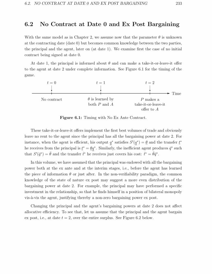
6.2. NO CONTRACT AT DATE 0 AND EX POST BARGAINING 233
6.2 No Contract at Date 0 and Ex Post Bargaining
With the same model as in Chapter 2, we assume now that the parameter θ is unknown
at the contracting date (date 0) but becomes common knowledge between the two parties,
the principal and the agent, later on (at date 1). We examine first the case of no initial
contract being signed at date 0.
At date 1, the principal is informed about θ and can make a take-it-or-leave-it offer
to the agent at date 2 under complete information. See Figure 6.1 for the timing of the
game.
- Time
t = 0 t = 1 t = 2
? ??
No contract θ is learned by
both P and AP makes a
take-it-or-leave-itoffer to A
Figure 6.1: Timing with No Ex Ante Contract.
These take-it-or-leave-it offers implement the first best volumes of trade and obviously
leave no rent to the agent since the principal has all the bargaining power at date 2. For
instance, when the agent is efficient, his output q∗ satisfies S ′(q∗) = θ and the transfer t∗
he receives from the principal is t∗ = θq∗. Similarly, the inefficient agent produces q∗ such
that S ′(q∗) = θ and the transfer t∗ he receives just covers his cost: t∗ = θq∗.
In this volume, we have assumed that the principal was endowed with all the bargaining
power both at the ex ante and at the interim stages, i.e., before the agent has learned
the piece of information θ or just after. In the non-verifiability paradigm, the common
knowledge of the state of nature ex post may suggest a more even distribution of the
bargaining power at date 2. For example, the principal may have performed a specific
investment in the relationship, so that he finds himself in a position of bilateral monopoly
vis-a-vis the agent, justifying thereby a non-zero bargaining power ex post.
Changing the principal and the agent’s bargaining powers at date 2 does not affect
allocative efficiency. To see that, let us assume that the principal and the agent bargain
ex post, i.e., at date t = 2, over the entire surplus. See Figure 6.2 below.

234 CHAPTER 6. NON-VERIFIABILITY
- Time
t = 0 t = 1 t = 2
? ??
No contract θ is learned by
both P and A
Bargaining
between P and Aover (t, q)
Figure 6.2: Timing with No Ex Ante Contract and Ex Post Bargaining.
To model this bargaining, we use the cooperative Nash bargaining solution with the
principal and the agent having now equal weights in the negotiation. In state θ, they
agree on a transfer t and production q which are solutions to the following problem:
(P ) : max{(q,t)}
(S(q)− t)(t− θq).
We easily find that the Nash bargaining solution consists of the first best output q∗(θ)and a transfer tNB(θ) which satisfy:
tNB(θ) =S(q∗(θ)) + θq∗(θ)
2, (6.1)
and
S ′(q∗(θ)) = θ. (6.2)
As a result, both the principal and the agent receive an equal share of the first-best
gains from trade. Denoting respectively by V NB(θ) and UNB(θ) the principal and the
agent’s shares of the surplus, we have thus:
V NB(θ) = UNB(θ) =1
2(S(q∗(θ))− θq∗(θ)) =
1
2W ∗(θ), (6.3)
where W ∗(θ) is the first best surplus in state θ.
Hence, waiting for date t = 2 to contract is detrimental to the principal if he loses
some bargaining power ex post. This justifies that the principal may prefer to offer a
contract at the ex ante stage.
Remark: Similar results would also hold with any kind of cooperative or non-cooperative
bargaining solution like the Rubinstein (1982) alternative offers bargaining game. The
particular way of splitting the ex post surplus has no allocative impact. The volume of
trade remains always at its first best value.
6.3 Incentive Compatible Contract
Instead of waiting for the realization of the state of nature, the principal can offer to the
agent, at the ex ante stage (date 0), a contract which may ensure ex post efficiency under
some rather weak conditions as we see below.

6.3. INCENTIVE COMPATIBLE CONTRACT 235
This contract can only be written in terms of the verifiable variables available to the
trading partners at date 0, namely the transfer t and the production q. For instance, a
contract saying “If state θ realizes, the agent must produce q∗(θ) and be paid t∗(θ) by the
principal” cannot be enforced because the state of nature θ is not verifiable at the ex
post contracting stage and consequently cannot be written into a contract. However, a
nonlinear price t(q) or a menu {(t, q); (t, q)} are feasible instruments at the ex ante stage.
When he accepts such a contract, the agent anticipates that his choice of outputs q(θ)
in state θ will satisfy the following constraints:
t(q(θ))− θq(θ) ≥ t(q)− θq, (6.4)
for all q where t(·) is defined and all θ in Θ.
These constraints are the same as the standard incentive compatibility constraints
highlighted in Chapter 2 as the reader will have recognized. Henceforth, there is a formal
correspondence between the case where contracting takes place under asymmetric infor-
mation between the principal and the agent and the case of ex ante contracting when the
state of nature is not verifiable. The Revelation Principle also applies in this context and
the class of direct revelation mechanisms of the form {(t, q); (t, q)} is enough to describe
all feasible contracts which command trade at date 2 and which can be signed at date
0 between the principal and the agent. Pushing this analogy, we call from now on these
contracts incentive compatible contracts.
The benefit of such incentive compatible contracts is that there is no need for the
principal to act ex post (i.e., at date 2) as shown in Figure 6.3 below. The fact that the
principal knows θ ex post is not used in such a mechanism. The mechanism is thus not
very demanding on the communication side.
- Time
t = 0 t = 1 t = 2
? ??
P offers a menu{(t, q); (t, q)} to A
θ is learned by
both P and AA chooses an
element of the menu.P does not act.
Figure 6.3: Timing with Ex Ante Contracting and Non-verifiability.
We already know from Section 2.12.1 that the first best outcome can still be achieved
with ex ante contracting provided that the agent is risk neutral in a two type environment.
Note nevertheless that the transfers with ex ante contracting are different from those
obtained with no contract at date 0, as we can easily observe by comparing the results of
Sections 2.12.1 and 6.2.1. The reason for this difference is simple. With no contract at
236 CHAPTER 6. NON-VERIFIABILITY
all, the transfers t∗ = θq∗ and t∗ = θq∗ which are offered by the principal at date 2 are no
longer incentive compatible2 as it is requested with ex ante contracting.
However, this result generalizes to several types and more general utility functions
U = t − C(q, θ) for the agent only if the Spence-Mirrlees condition Cθq > 0 is satisfied.
Otherwise, the second-order conditions for incentive compatibility may create some inef-
ficiencies and may require some bunching as in the case of non-responsiveness of Section
2.11. The superiority of ex ante contracting over ex post contracting with less bargaining
power is then questionable.
Similarly, as also shown in Section 2.12, ex ante contracting fails also to achieve ef-
ficiency when the agent is risk averse. The non-verifiability of the state of nature may
conflict with the insurance concerns of the agent if the principal offers an incentive com-
patible contract. Section 2.12.2 provides, therefore, also an analysis of the efficiency loss
incurred when ex ante contracting limited to incentive compatible contracts takes place
in a world of non-verifiability and risk aversion.
6.4 Nash Implementation
In Section 6.3, we have just seen how the principal and the agent can achieve ex post
efficiency through an ex ante contract when they are both risk neutral. This contract uses
only the agent’s message but fails to achieve efficiency when the agent is risk averse or when
non-responsiveness occurs. We propose now a slightly more complicated implementation
of the ex post efficient allocation which works also in these cases. The new feature of this
implementation comes from the fact that both the principal and the agent must send a
report on the state of nature at date 2. Requesting both the principal and the agent to
report the state of nature moves us somewhat beyond the focus of this volume which has
been to emphasize incentive mechanisms in a single agent environment. However, under
complete information, the analysis of two-agent mechanisms is relatively straightforward.
In this context, a general mechanism should involve two message spaces, one for the
principal, say Mp, and one for the agent Ma. Still denoting by A the set of feasible
allocations, we have the following definition.
Definition 6.1 : A mechanism is a pair of message spaces Ma and Mp and a mapping
g(·) from M = Ma×Mp into A which writes as g(ma,mp) = {q(ma,mp), t(ma,mp)} for
all pairs (ma,mp) belonging to M.
Let us assume that the principal and the agent have respective utility functions V =
2Indeed, we have 0 = t∗ − θq∗ < t∗ − θq∗ = ∆θq∗.

6.4. NASH IMPLEMENTATION 237
S(q, θ) − t and U = t − C(q, θ). In this context, the first-best allocation rule a∗(θ) =
(t∗(θ), q∗(θ)) is such that:
Sq(q∗(θ), θ) = Cq(q
∗(θ), θ) (6.5)
and
t∗(θ) = C(q∗(θ), θ). (6.6)
When the players face a mechanism, a Nash equilibrium (m∗a(θ),m
∗p(θ)) of their mes-
sages satisfies the following incentive conditions: For the principal,
S(q(m∗a(θ),m
∗p(θ)), θ)− t(m∗
a(θ),m∗p(θ)) ≥ S(q(m∗
a(θ), mp), θ)− t(m∗a(θ), mp), (6.7)
for all θ in Θ and mp in Mp;
and for the agent,
t(m∗a(θ),m
∗p(θ))− C(q(m∗
a(θ),m∗p(θ)), θ) ≥ t(ma,m
∗p(θ))− C(q(ma,m
∗p(θ)), θ), (6.8)
for all θ in Θ and ma in Ma.
When the principal conjectures that the agent’s reporting strategy is given by m∗a(θ)
in state θ, he reports his best response m∗p(θ). Similarly, the agent’s report strategy m∗
a(θ)
is a best response to the principal’s behavior. Then, the pair of strategies (m∗a(θ),m
∗p(θ))
forms a Nash equilibrium of the game form induced by the mechanism g(·).3
An allocation rule a(θ) from Θ to A is implemented in Nash equilibrium by a mecha-
nism (M, g(·)) if there exists a Nash equilibrium (m∗a(θ),m
∗p(θ)) in M such that a(θ) =(
q(m∗a(θ),m
∗p(θ)), t(m
∗a(θ),m
∗p(θ))
)for all θ in Θ.
When the message spaces Ma and Mp are reduced to the set of possible types Θ, we
have the following definition:
Definition 6.2 : A direct revelation mechanism is a mapping g(·) from Θ2 to A which
writes as g(θa, θp) = {q(θa, θp), t(θa, θp)} where θa (resp. θp) is the agent (resp. principal)’s
report in Θ.
We have also:
Definition 6.3 : A direct revelation mechanism g(·) is truthful if it is a Nash equilibrium
for the agent and the principal to report truthfully the state of nature.
3We focus on pure-strategy equilibria for the sake of simplicity, but without loss of generality.

238 CHAPTER 6. NON-VERIFIABILITY
Denoting by Ng(θ) the set of Nash equilibria of the direct revelation mechanism g(·)in state θ, we have the following definition:
Definition 6.4 : The allocation a(θ) is implementable in Nash equilibrium by the direct
revelation mechanism g(·) if the pair of truthful strategies of the principal and the agent
forms a Nash equilibrium of g(·) ((θ, θ) ∈ Ng(θ) for all θ in Θ) such that a(θ) = g(θ, θ)
for all θ in Θ.
Truthful direct revelation mechanisms must thus satisfy the following Nash incentive
constraints:
S(q(θ, θ), θ)− t(θ, θ) ≥ S(q(θ, θp), θ)− t(θ, θp) (6.9)
for all (θ, θp) in Θ2,
and
t(θ, θ)− C(q(θ, θ), θ) ≥ t(θa, θ)− C(q(θa, θ), θ), (6.10)
for all (θa, θ) in Θ2.
We can now prove a new version of the Revelation Principle.
Proposition 6.1 : Any allocation rule a(θ) which is implemented in Nash equilibrium by
a mechanism (M, g(·)) can also be implemented in Nash equilibrium by a truthful direct
revelation mechanism.
Proof: The mechanism (M, g(·)) induces an allocation a(θ) = (q(m∗a(θ),m
∗p(θ)), t(m∗
a(θ),m∗p(θ))).
Let us define a direct mechanism g(·) from Θ2 into A such that g = g ◦ m∗ where
m∗ = (m∗a,m
∗p). For all states of nature θ, we have thus g(θ) = (q(θ), t(θ)) ≡ g(m∗(θ)) =
(q(m∗a(θ),m
∗p(θ)), t(m
∗a(θ),m
∗p(θ))). We check that it is a Nash equilibrium for the players
to report the truth when they face the direct revelation mechanism g(·). For the principal,
we have indeed:
S(q(θ, θ), θ)− t(θ, θ) = S(q(m∗a(θ),m
∗p(θ)), θ)− t(m∗
a(θ),m∗p(θ))
≥ S(q(m∗a(θ), mp), θ)− t(m∗
a(θ), mp)
for all mp in Mp and for all θ in Θ.
Taking mp = m∗p(θ
′) for any θ′ in Θ, we obtain:
S(q(θ, θ), θ)− t(θ, θ) ≥ S(q(m∗a(θ),m
∗p(θ
′)), θ)− t(m∗a(θ),m
∗p(θ
′))
for all (θ, θ′) in Θ2.
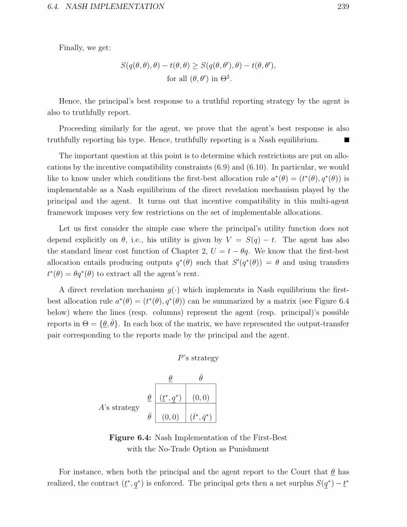
6.4. NASH IMPLEMENTATION 239
Finally, we get:
S(q(θ, θ), θ)− t(θ, θ) ≥ S(q(θ, θ′), θ)− t(θ, θ′),
for all (θ, θ′) in Θ2.
Hence, the principal’s best response to a truthful reporting strategy by the agent is
also to truthfully report.
Proceeding similarly for the agent, we prove that the agent’s best response is also
truthfully reporting his type. Hence, truthfully reporting is a Nash equilibrium.
The important question at this point is to determine which restrictions are put on allo-
cations by the incentive compatibility constraints (6.9) and (6.10). In particular, we would
like to know under which conditions the first-best allocation rule a∗(θ) = (t∗(θ), q∗(θ)) is
implementable as a Nash equilibrium of the direct revelation mechanism played by the
principal and the agent. It turns out that incentive compatibility in this multi-agent
framework imposes very few restrictions on the set of implementable allocations.
Let us first consider the simple case where the principal’s utility function does not
depend explicitly on θ, i.e., his utility is given by V = S(q) − t. The agent has also
the standard linear cost function of Chapter 2, U = t − θq. We know that the first-best
allocation entails producing outputs q∗(θ) such that S ′(q∗(θ)) = θ and using transfers
t∗(θ) = θq∗(θ) to extract all the agent’s rent.
A direct revelation mechanism g(·) which implements in Nash equilibrium the first-
best allocation rule a∗(θ) = (t∗(θ), q∗(θ)) can be summarized by a matrix (see Figure 6.4
below) where the lines (resp. columns) represent the agent (resp. principal)’s possible
reports in Θ = {θ, θ}. In each box of the matrix, we have represented the output-transfer
pair corresponding to the reports made by the principal and the agent.
P ’s strategy
θ θ
θ (t∗, q∗) (0, 0)A’s strategy
θ (0, 0) (t∗, q∗)
Figure 6.4: Nash Implementation of the First-Best
with the No-Trade Option as Punishment
For instance, when both the principal and the agent report to the Court that θ has
realized, the contract (t∗, q∗) is enforced. The principal gets then a net surplus S(q∗)− t∗

240 CHAPTER 6. NON-VERIFIABILITY
and the agent gets t∗ − θq∗ if the true state of nature is θ. If they disagree the no-trade
option is enforced, with no output being produced and no transfer being made.
The important point to note is that the same game form must be played by the
agent and the principal whatever the true state of nature θ. Indeed, the state of na-
ture being nonverifiable, the transfers and outputs in each box of the matrix cannot
be made contingent on it. The goal of this mechanism is to ensure that there exists
a truthful Nash equilibrium in each state θ which implements the first-best allocation
a∗(θ) = (t∗(θ), q∗(θ)).
Let us check that telling the truth is a Nash equilibrium of the direct revelation
mechanism g(·) in each state of nature. Consider first state θ. Given that the agent
reports θ, the principal gets S(q∗) − t∗ = S(q∗) − θq∗ by reporting the truth and zero
otherwise. By assumption, trade is valuable when θ realizes (S(q∗)− θq∗ > 0) and telling
the truth is a best response for the principal. The agent is indifferent between telling the
truth or not when the principal reports θ since t∗ − θq∗ = 0. Hence, he weakly prefers to
tell the truth as a best response.
Consider now state θ. Given that the agent reports θ, the principal gets S(q∗)− t∗ =
S(q∗) − θq∗ by reporting the truth and zero otherwise. By assumption trade is valuable
also when θ realizes (S(q∗) − θq∗ > 0). Telling the truth is a best response for the
principal. Similarly, the agent is indifferent between telling the truth or not when the
principal reports truthfully since t∗ − θq∗ = 0. He weakly prefers to tell the truth.
Importantly, note that, when θ realizes, the pair of truthful strategies is not the
unique Nash equilibrium of the direct mechanism g(·). (θ, θ) is indeed another Nash
equilibrium. The agent strictly gains from misreporting if the principal does so since
t∗ − θq∗ = ∆θq∗ > 0. Also, the principal prefers to report θ if the agent does so since
S(q∗)− t∗ > 0.
There are two possible attitudes vis-a-vis this multiplicity problem. First, one may
forget about it and argue that telling the truth should be a focal equilibrium. This is a
relatively shaky argument in the absence of a theory of equilibrium selection. Moreover,
some authors have argued in related models that the non-truthful equilibrium may Pareto
dominate the truthful one from the players’ point of view.4 This second argument is less
effective in our context since the two equilibria cannot be Pareto-ranked: in the non-
truthful equilibrium the agent does better than in the truthful one, but the principal does
worse.
The second possible attitude towards the multiplicity of equilibria is to take it seri-
ously and to look for mechanisms which ensure that the first-best allocation is uniquely
4See Demski and Sappington (1984) for such a model.

6.4. NASH IMPLEMENTATION 241
implementable.
Definition 6.5 : The first-best allocation rule a∗(θ) is uniquely implementable in Nash
equilibrium by the mechanism (M, g(·)) if the mechanism has a unique Nash equilibrium
for each θ in Θ and it induces the allocation a∗(θ).
In the definition above, we do not restrict a priori the mechanism g(·) to be a direct
one. It could well be that the cost of obtaining unique implementation is to expand a
little bit the space of messages that the agent and the principal use to communicate with
the Court. Such extensions are often used in multi-agent (more than three) frameworks.
In our principal-agent model, those extensions are often not needed provided that one
defines conveniently the out-of-equilibrium path punishments.
For the time being, let us consider a direct revelation mechanism as in Figure 6.5
below.
P ’s strategy
θ θ
θ (t∗, q∗) (t2, q2)A’s strategy
θ (t1, q1) (t∗, q∗)
Figure 6.5: Nash Implementation of the First-Best
with More General Punishments.
The outcomes (t1, q1) and (t2, q2) may be different from the no-trade option in order
to give more flexibility to the Court in designing off-the-equilibrium path punishments
ensuring both truthful revelation and uniqueness of the equilibrium.
The conditions for having a truthful Nash equilibrium in state θ are: For the principal
S(q∗)− t∗ > S(q2)− t2, (6.11)
and for the agent
0 = t∗ − θq∗ > t1 − θq1. (6.12)
Similarly, the conditions for having a truthful Nash equilibrium in state θ are: For the
principal
S(q∗)− t∗ > S(q1)− t1, (6.13)

242 CHAPTER 6. NON-VERIFIABILITY
and for the agent
0 = t∗ − θq∗ > t2 − θq2. (6.14)
Let us now turn to the conditions ensuring that there is no non-truthful pure-strategy
Nash equilibrium in either state of nature. Let us consider a possible non-truthful equi-
librium (θ, θ) when state θ realizes. Given that (6.13) is needed to satisfy the principal’s
incentive constraint in state θ, the only way to break the possible equilibrium is to have:
t∗ − θq∗ < t2 − θq2. (6.15)
Let us consider also a possible non-truthful pure-strategy Nash equilibrium (θ, θ) when
state θ realizes. Given that (6.11) is needed to ensure the principal’s incentive constraint
in state θ, the only way to break the possible equilibrium is to have:
t∗ − θq∗ < t1 − θq1. (6.16)
A truthful direct revelation mechanism g(·) which uniquely implements the first-best
as a Nash equilibrium exists when the conditions (6.11) to (6.16) are all satisfied by a
pair of off-the-equilibrium path contracts (t1, q1) and (t2, q2). We have:
Proposition 6.2 : A truthful direct revelation mechanism g(·) which uniquely imple-
ments in Nash equilibrium the first-best allocation rule a∗(θ) exists.
Proof: The clearest way of doing this proof is to draw a picture. In Figure 6.6 below, we
have represented the first-best allocation a∗(θ) and the possible punishments (t1, q1) and
(t2, q2).

6.4. NASH IMPLEMENTATION 243
-
6
""
""
""
""
""
""
""
""
""
""
""
""
""
""
""
¢¢¢¢¢¢¢¢¢¢¢¢¢¢¢¢¢¢¢¢¢¢¢¢¢¢¢¢
•B∗
•A∗
q∗
t∗
q∗
t∗
t
q""¦¦6
E
C
D
U∗ = 0 = t− θq
´´
´´
´
U∗ = t− θq = 0
W ∗ = S(q)− t
W ∗ = S(q)− t
¢¢
¢¢
¢¢
¢¢
¢¢
¢¢
¢¢
¢¢
¢¢
¢¢
¢¢"""""""""""""""""""""""
ll
ZZ
ZZ
bb
HHH
HHHHH
HHHHHHH
HHHHHHHHH
HHHHHHHHHHH
HHHHHHHHHHHHH
ZZ
ZZ
ZZZ
""
ZZ~
BBN
@@@I
©©
@@
@@I
""""""""""""""""""""""""""
Figure 6.6: Off-The-Equilibrium Path Punishments.
In the figure, the indifference curves of the principal are tangent to the zero-profit lines
of the agent in each state of nature. First, the θ-agent incentive compatibility constraint
(6.12) and (6.16) define a subset C where (t1, q1) may lie (crossed area in Figure 6.6).
Within this subset, the principal’s incentive constraint (6.13) further reduces the set of
possible punishments (t1, q1) to the area E close to the origin (shaded area in Figure 6.6).
This set is non-empty since the principal’s indifference curve W ∗ = S(q)− t does not go
through the origin when trade is valuable in state θ(S(q∗)− t∗ > 0).
Similarly, the agent’s incentive constraints (6.14) and (6.15) define a subset D of
possible values for the punishment (t2, q2) (crossed area in Figure 6.6). In Figure 6.6, this
full set satisfies the principal’s incentive compatibility constraint (6.11). More generally,
by strict concavity of the principal’s indifference curve W ∗ = S(q)− t going through B∗,there exists a non-empty subset of D which lies strictly above this indifference curve. All
those points lie obviously above the principal’s indifference curve W ∗ = S(q) − t going
through A∗.
Proposition 6.2 yields a quite striking result. It says that direct revelation mechanisms

244 CHAPTER 6. NON-VERIFIABILITY
are enough to ensure always efficiency if the Court can design punishments in a clever way.
There is no need to use more complex mechanisms in this simple and rather structured
principal-agent model.
More generally, one may wonder if the requirement of unique Nash implementation
imposes some structure on the set of allocation rules a(θ) = (t(θ), q(θ)) which can be
implemented this way. Indeed, this structure exists. Before describing it, we need another
definition that we cast in the general case where V = S(q, θ)− t and U = t− C(q, θ).
Definition 6.6 : An allocation rule a(θ) = (t(θ), q(θ)) is monotonic if and only if for
any θ in Θ such that a(θ) 6= a(θ′) for some θ′ in Θ, there exists an allocation (t, q) such
that one of the two conditions below is true:
(P )
S(q(θ), θ)− t(θ) ≥ S(q, θ)− tand
S(q, θ′)− t > S(q(θ), θ′)− t(θ),
or
(A)
t(θ)− C(q(θ), θ) ≥ t− C(q, θ)and
t− C(q, θ′) > t(θ)− C(q(θ), θ′).
These inequalities have a simple meaning.5 The allocation rule a(·) selects the pair
a(θ) = (t(θ), q(θ)) in state θ and not in state θ′, if there exists another allocation (t, q)
such that either the principal or the agent prefers this allocation to a(θ) when the state
of nature is θ′.
Under the assumptions of Proposition 6.2, the first-best allocation rule a∗(·) is mono-
tonic. Indeed, first we note that a∗(θ) 6= a∗(θ). Second, the principal’s utility function
being independent of θ, there does not exist any allocation (t, q) such that condition (P )
holds. Lastly, there exist (t, q) such that condition (A) holds. In state θ, the set of such
pairs is contains the set C in Figure 6.6. In state θ, it is the set D.
The monotonicity of allocation rules is an important property which follows immedi-
ately from unique implementation as it is shown in Proposition 6.3 below.
Proposition 6.3 : Consider an allocation rule a(·) which is uniquely implemented in
Nash equilibrium by a mechanism (M, g(·)); then the allocation rule a(·) is monotonic.
5An alternative definition which explains better the expression “monotonicity” is intuitively as follows.If a(θ) is selected in state θ and if the allocation a(θ) “progresses” in the preferences of both players inanother state of nature θ′, a(θ) must also be chosen in state θ′.

6.4. NASH IMPLEMENTATION 245
Proof: The mechanism (M, g(·)) uses the message spaces Ma and Mp. If the allocation
rule a(·) is uniquely implementable in Nash equilibrium by g(·), we know that, in state θ,
there exists a pair of strategies (m∗a(θ),m
∗p(θ)) such that (q(θ), t(θ)) = (q(m∗
a(θ),m∗p(θ)),
t(m∗a(θ), m
∗p(θ))) and:
S(q(m∗a(θ),m
∗p(θ)), θ)− t(m∗
a(θ),m∗p(θ)) ≥ S(q(m∗
a(θ), mp), θ)− t(m∗a(θ), mp) (6.17)
for all mp it Mp;
t(m∗a(θ),m
∗p(θ))− C(q(m∗
a(θ),m∗p(θ)), θ) ≥ t(ma,m
∗p(θ))− C(q(ma,m
∗p(θ)), θ)(6.18)
for all ma in Ma.
Moreover, a(θ) being different from a(θ′) for a θ′ different from θ, a(θ) is not a Nash
equilibrium in state θ′. This means that either the principal, or the agent, finds then
strictly better to send a message mp rather than m∗p(θ) or ma rather than m∗
a(θ). For the
principal this means that:
S(q(θ), θ′)− t(θ) < S(q(m∗a(θ), mp), θ
′)− t(m∗a(θ), mp). (6.19)
For the agent this means that
t(θ)− C(q(θ), θ′) < t(ma,m∗p(θ))− C(q(ma,m
∗p(θ)), θ
′). (6.20)
In each case show that the allocation rule a(·) is monotonic. Take (t, q) = (t(m∗a(θ), mp),
q(m∗a(θ), mp))) in the first case (principal’s deviation) and (t, q) = (t(ma,m
∗p(θ)), q(ma,m
∗p(θ)))
in the second case (agent’s deviation).
The intuitive meaning of Proposition 6.3 is rather clear. In order to prevent an allo-
cation implemented in one state of nature θ to be also chosen in another state θ′, either
the principal or the agent must deviate and choose another message in state θ′. Hence,
the mechanism g(·) which uniquely implements the allocation rule a(·) must include an
allocation (t, q) which is worse than (t(θ), q(θ)) for both agents in state θ, but better for
at least one in state θ′. In this case, the latter player’s preferences are reversed between
states θ and θ′, breaking a possible equilibrium which would implement a(θ) also in state
θ′.
The monotonicity property is a necessary condition satisfied by an allocation
rule which is uniquely implementable in Nash equilibrium. The remaining question is
to know how far away this property is from sufficiency. With more than two agents
(n ≥ 3), Maskin (1999) shows that monotonicity plus another property, no veto power,6
6This property says that whenever n − 1 agents prefer an allocation to all others in one state ofnature, the nth agent cannot veto it and this allocation belongs to the allocation rule. The no veto powerproperty is a rather innocuous property to satisfy in economic contexts with more than two agents.

246 CHAPTER 6. NON-VERIFIABILITY
is also sufficient for unique Nash implementation. With two agents only, Dutta and Sen
(1991) and Moore and Repullo (1990) have provided necessary and sufficient conditions
for unique Nash implementation in more general environments than those analyzed in
this chapter.
6.5 Subgame Perfect Implementation
From Proposition 6.3, a necessary condition for unique Nash implementation is that an
allocation rule a(·) be monotonic. Any allocation rule which fails to be monotonic will also
fail to guarantee unique Nash implementation. Then, one may wonder if refinements of the
Nash equilibrium concept can be used to still ensure unique implementation. A natural
refinement is to move to a game with sequential moves where the principal and the agent
take turn in sending messages to the Court. An allocation rule a(θ) is implementable
uniquely in subgame perfect equilibrium by a mechanism g(·) if the unique subgame
perfect equilibrium yields allocation a(θ) in any state θ.
Instead of presenting the general theory of subgame perfect implementation which is
quite complex, we propose a simple example showing the mechanics of the procedure.
Let us first single out a principal-agent setting where the first-best allocation rule is non-
monotonic. Consider a principal with utility function V = S(q) − t independent of the
state of nature θ. For simplicity, we will assume that S(q) = µq − λq2
2where µ and λ are
common knowledge. The agent has instead a utility function U = t − θ1q − θ2q2
2where
θ = (θ1, θ2) is the bidimensional state of nature.
First-best outputs q∗(θ1, θ2) are given by the first-order conditions S ′(q∗(θ1, θ2)) =
θ1 + θ2q∗(θ1, θ2). We immediately find that q∗(θ1, θ2) = µ−θ1
λ+θ2.
We assume that each parameter θi belongs to Θ = {θ, θ}. A priori, there are 4 possible
states of nature and 4 first-best outputs. Assuming that µ−θλ+θ
= µ−θλ+θ
, i.e., µ − λ = θ + θ,
we are left with three first-best outputs q∗ = µ−θλ+θ
, q∗ = µ−θλ+θ
= 1 and q∗ = µ−θλ+θ
that we
assume to be positive.
Of course, even if the production level is the same in states (θ, θ) and (θ, θ), the agent
has different costs and should receive different transfers t∗1 and t∗2 from the principal. We
denote by t∗ and t∗ the transfers in the other states of nature.
In Figure 6.7, we have represented the first-best allocations corresponding to the dif-
ferent states of nature.
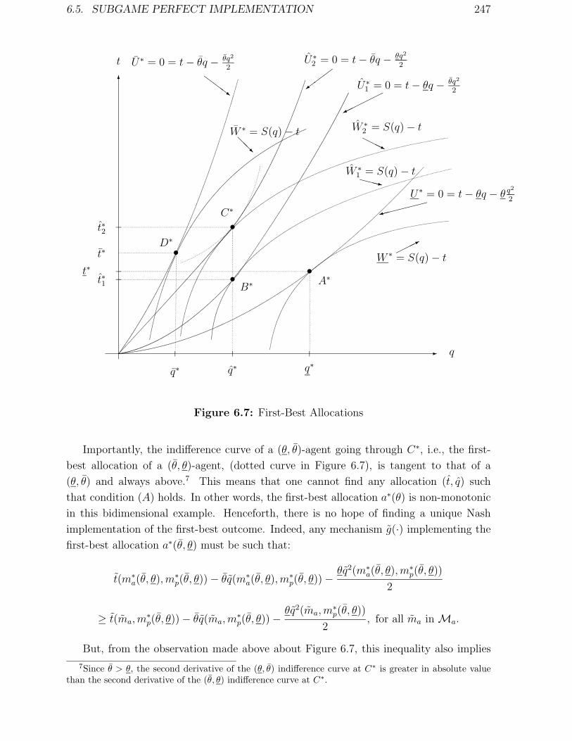
6.5. SUBGAME PERFECT IMPLEMENTATION 247
-
6
•
•
C∗
B∗
q∗
t∗1
t∗2
t
q
••
q∗
t∗A∗
t∗
q∗
D∗
U∗ = 0 = t− θq − θq2
2
ZZZ~
U∗2 = 0 = t− θq − θq2
2½
½½= U∗
1 = 0 = t− θq − θq2
2©©©©©¼
W ∗ = S(q)− t@@R
W ∗2 = S(q)− tHHHj
W ∗1 = S(q)− tXXXz
W ∗ = S(q)− t©©©*
U∗ = 0 = t− θq − θ q2
2»»»»»»9
Figure 6.7: First-Best Allocations
Importantly, the indifference curve of a (θ, θ)-agent going through C∗, i.e., the first-
best allocation of a (θ, θ)-agent, (dotted curve in Figure 6.7), is tangent to that of a
(θ, θ) and always above.7 This means that one cannot find any allocation (t, q) such
that condition (A) holds. In other words, the first-best allocation a∗(θ) is non-monotonic
in this bidimensional example. Henceforth, there is no hope of finding a unique Nash
implementation of the first-best outcome. Indeed, any mechanism g(·) implementing the
first-best allocation a∗(θ, θ) must be such that:
t(m∗a(θ, θ),m
∗p(θ, θ))− θq(m∗
a(θ, θ),m∗p(θ, θ))−
θq2(m∗a(θ, θ),m
∗p(θ, θ))
2
≥ t(ma,m∗p(θ, θ))− θq(ma,m
∗p(θ, θ))−
θq2(ma,m∗p(θ, θ))
2, for all ma in Ma.
But, from the observation made above about Figure 6.7, this inequality also implies
7Since θ > θ, the second derivative of the (θ, θ) indifference curve at C∗ is greater in absolute valuethan the second derivative of the (θ, θ) indifference curve at C∗.

248 CHAPTER 6. NON-VERIFIABILITY
that:
t(m∗a(θ, θ),m
∗p(θ, θ))− θq(m∗
a(θ, θ),m∗p(θ, θ))−
θq2(m∗a(θ, θ),m
∗p(θ, θ))
2
≥ t(ma,m∗p(θ, θ))− θq(ma,m
∗p(θ, θ))−
θq2(ma,m∗p(θ, θ))
2, for all ma in Ma.
Since the principal’s utility function does not depend directly on θ, the pair of strate-
gies (m∗a(θ, θ); m
∗p(θ, θ)) which implements the allocation a∗(θ, θ) = (t2, q
∗) remains an
equilibrium in state (θ, θ).
Let us now turn to a possible unique implementation using a three stage extensive
form mechanism and the more stringent concept of subgame perfection.
The reader should be convinced that there is not too much problem in eliciting the
preferences of the agent in states (θ, θ) and (θ, θ). Hence, we will focus on a “reduced”
extensive form which is enough to highlight the logic of subgame perfect implementation.
The objective of this extensive form is to have the agent truthfully reveal the state of
nature when (θ, θ) or (θ, θ) occurs.
In Figure 6.8 below, we have represented such an extensive form.
A
¢¢
¢¢
¢¢
¢¢
AAAAAAAA
(t1, q1) (t2, q2)
AA
AA
AA
AA
P
¢¢
¢¢
¢¢
¢¢
(t∗2, q∗)
chooses chooses
AA
AA
AA
AA
A
¢¢
¢¢
¢¢
¢¢
(t∗1, q∗)
agrees challenges
announces announces
(θ, θ)(θ, θ)
•
•
Figure 6.8: Subgame Perfect Implementation.
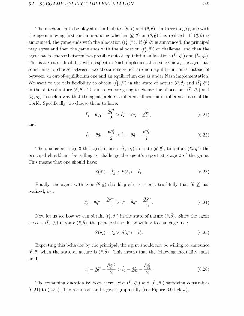
6.5. SUBGAME PERFECT IMPLEMENTATION 249
The mechanism to be played in both states (θ, θ) and (θ, θ) is a three stage game with
the agent moving first and announcing whether (θ, θ) or (θ, θ) has realized. If (θ, θ) is
announced, the game ends with the allocation (t∗1, q∗). If (θ, θ) is announced, the principal
may agree and then the game ends with the allocation (t∗2, q∗) or challenge, and then the
agent has to choose between two possible out-of-equilibrium allocations (t1, q1) and (t2, q2).
This is a greater flexibility with respect to Nash implementation since, now, the agent has
sometimes to choose between two allocations which are non-equilibrium ones instead of
between an out-of-equilibrium one and an equilibrium one as under Nash implementation.
We want to use this flexibility to obtain (t∗1, q∗) in the state of nature (θ, θ) and (t∗2, q
∗)in the state of nature (θ, θ). To do so, we are going to choose the allocations (t1, q1) and
(t2, q2) in such a way that the agent prefers a different allocation in different states of the
world. Specifically, we choose them to have:
t1 − θq1 − θq21
2> t2 − θq2 − θ
q22
2, (6.21)
and
t2 − θq2 − θq22
2> t1 − θq1 − θq2
1
2. (6.22)
Then, since at stage 3 the agent chooses (t1, q1) in state (θ, θ), to obtain (t∗2, q∗) the
principal should not be willing to challenge the agent’s report at stage 2 of the game.
This means that one should have:
S(q∗)− t∗2 > S(q1)− t1. (6.23)
Finally, the agent with type (θ, θ) should prefer to report truthfully that (θ, θ) has
realized, i.e.:
t∗2 − θq∗ − θq∗2
2> t∗1 − θq∗ − θq∗2
2. (6.24)
Now let us see how we can obtain (t∗1, q∗) in the state of nature (θ, θ). Since the agent
chooses (t2, q2) in state (θ, θ), the principal should be willing to challenge, i.e.:
S(q2)− t2 > S(q∗)− t∗2. (6.25)
Expecting this behavior by the principal, the agent should not be willing to announce
(θ, θ) when the state of nature is (θ, θ). This means that the following inequality must
hold:
t∗1 − θq∗ − θq∗2
2> t2 − θq2 − θq2
2
2. (6.26)
The remaining question is: does there exist (t1, q1) and (t2, q2) satisfying constraints
(6.21) to (6.26). The response can be given graphically (see Figure 6.9 below).

250 CHAPTER 6. NON-VERIFIABILITY
-
6
•
•
C∗
B∗
q∗
t∗1
t∗2
• (t2, q2)
• (t1, q1)
U∗2 = t− θq − θq2
2J
JJ U∗1 = t− θq − θq2
2AAU
W ∗1 = S(q)− t¡
¡µ
W ∗2 = S(q)− t½
½>
t
q
Figure 6.9: Subgame-Perfect Implementation.
By definition, (t1, q1) (resp. (t2, q2)) should be above (resp. below) the principal’s
indifference curve going through C∗. Note that for q > q∗, the indifference curves of an
agent with (θ, θ) have a greater slope than those of an agent with type (θ, θ). This helps
to construct very easily the out-of-equilibrium allocations (t1, q1) and (t2, q2) as in Figure
6.9.
Remark: Subgame perfect implementation is beautiful and attractive but it should be
noted that it has been sometimes criticized because it relies excessively on rationality.
The kind of problem at hand can be illustrated with our example of Figure 6.8. Indeed,
when state (θ, θ) realizes and the principal has to decide to move at the second stage, he
knows that the agent has already made a suboptimal move. Why should he believe that
the agent will behave optimally at stage 3 as needed by subgame perfect implementation?
Moore and Repullo (1990) present a set of conditions ensuring subgame perfect
implementation in general environments, noticeably those with more than two agents. The
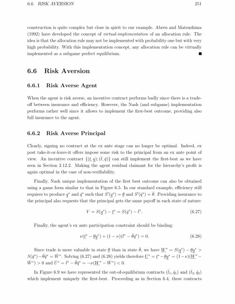
6.6. RISK AVERSION 251
construction is quite complex but close in spirit to our example. Abreu and Matsushima
(1992) have developed the concept of virtual-implementation of an allocation rule. The
idea is that the allocation rule may not be implemented with probability one but with very
high probability. With this implementation concept, any allocation rule can be virtually
implemented as a subgame perfect equilibrium.
6.6 Risk Aversion
6.6.1 Risk Averse Agent
When the agent is risk averse, an incentive contract performs badly since there is a trade-
off between insurance and efficiency. However, the Nash (and subgame) implementation
performs rather well since it allows to implement the first-best outcome, providing also
full insurance to the agent.
6.6.2 Risk Averse Principal
Clearly, signing no contract at the ex ante stage can no longer be optimal. Indeed, ex
post take-it-or-leave-it offers impose some risk to the principal from an ex ante point of
view. An incentive contract {(t, q); (t, q)} can still implement the first-best as we have
seen in Section 2.12.2. Making the agent residual claimant for the hierarchy’s profit is
again optimal in the case of non-verifiability.
Finally, Nash unique implementation of the first best outcome can also be obtained
using a game form similar to that in Figure 6.5. In our standard example, efficiency still
requires to produce q∗ and q∗ such that S ′(q∗) = θ and S ′(q∗) = θ. Providing insurance to
the principal also requests that the principal gets the same payoff in each state of nature:
V = S(q∗)− t∗ = S(q∗)− t∗. (6.27)
Finally, the agent’s ex ante participation constraint should be binding:
ν(t∗ − θq∗) + (1− ν)(t∗ − θq∗) = 0. (6.28)
Since trade is more valuable in state θ than in state θ, we have W ∗ = S(q∗) − θq∗ >
S(q∗)− θq∗ = W ∗. Solving (6.27) and (6.28) yields therefore U∗ = t∗−θq∗ = (1−ν)(W ∗−W ∗) > 0 and U∗ = t∗ − θq∗ = −ν(W ∗ − W ∗) < 0.
In Figure 6.9 we have represented the out-of-equilibrium contracts (t1, q1) and (t2, q2)
which implement uniquely the first-best. Proceeding as in Section 6.4, these contracts

252 CHAPTER 6. NON-VERIFIABILITY
must again satisfy the following constraints:
t1 − θq1 < t∗ − θq∗, (6.29)
t1 − θq1 > t∗ − θq∗, (6.30)
S(q∗)− t∗ > S(q1)− t1; (6.31)
and
t2 − θq2 < t∗ − θq∗, (6.32)
t2 − θq2 > t∗ − θq∗, (6.33)
S(q∗)− t∗ > S(q2)− t2. (6.34)
We let the reader check that the set E (crossed area) (resp. F (dotted area ◦))of possible values of (t1, q1) (resp. (t2, q2)) satisfying constraints (6.29) to (6.31) (resp.
(6.32)) to (6.34) can be represented as in Figure 6.10.
-
6
t
q!!!!!!!!!!!!!!!!!!!!!!!!!!!!!!!!!
!!!!!!!!!!!!!!!!!!!!!!!!!!!!!!!!!!!!
t∗
q∗
•
!!!!!!!!!!!!!!!!!!!!!!!!!!!!!!!!!!
¯¯¯¯¯¯¯¯¯¯¯¯¯¯¯¯¯¯¯¯¯¯¯¯¯¯¯¯¯¯¯
££££££££££££££££££££££££££££££££
•
q∗
t∗B∗
E
F
0 = t− θq
U∗ = t− θq
(t2, q2)
(t1, q1)
•
CCCCCCW
0 = t− θq@
@@I
W = S(q)− t½
½½>
U∗ = t− θqJJ
@@
@@@
@@@
@@
@@
@@
@@
@@
@
@@@
@@@@
@@@@e e
e eee e ee e
e eee
e
e e e ee ee
eeeee
ee e e e
e•
¯¯¯¯¯¯¯¯¯¯¯¯¯¯¯¯¯¯¯¯¯¯¯¯¯¯¯¯¯
Figure 6.10: Nash Unique Implementation with Risk Aversion.

6.7. CONCLUDING REMARKS 253
6.7 Concluding Remarks
The overall conclusion of this chapter is that the non-verifiability of the state of nature ex
ante is not enough to impose any transaction cost in contracting if the Court of Justice can
credibly enforce punishments out of the equilibrium path. The non-verifiability paradigm
becomes only useful under various incomplete contracting assumptions such as the inabil-
ity to commit to ex post inefficiency or the possibility of collusion in environments with
at least three agents.8
8See Volume III.

254 CHAPTER 6. NON-VERIFIABILITY

Chapter 7
Mixed Models
7.1 Introduction
The pure models of Chapter 2 for adverse selection, Chapter 4 for moral hazard and
Chapter 6 for the case of non-verifiability were highly stylized contracting settings. Each
of those models was aimed at capturing a single dimension of the incentive problems
that may be faced by a principal at the time of designing the contract of his agent. In
Chapters 2, 4 and 6 respectively, the analysis of each of these respective paradigms has
already provided a number of important insights which concern, on the one hand, the
conflict (if any) between allocative efficiency and the distribution of the gains from trade
and, on the other hand, the form of the optimal compensation schedule. Moreover, our
investigation of more complex models than those of Chapters 2 and 4 has also shown how
the insights gleaned from these simple models turn out to be quite robust to changes in
the economic environment.1
In real world settings, contracts are rarely designed with the objective of solving a
single dimension of the incentive problem. Most often, the principal’s control of the agent
requires to deal simultaneously with both adverse selection and moral hazard, or with
both the non-verifiability of the state of nature and moral hazard. The most important
question is thus to know how the agency costs due to the different paradigms interact.
More precisely, we would like to assess whether the lessons from the pure models continue
to hold in those more complex environments and, if they do not hold anymore, one would
like to understand in which directions those lessons should be modified.
This chapter is not aimed at giving a complete overview of the huge and extremely
heterogeneous literature which analyzes settings where several paradigms are simultane-
ously useful to understand the economic problem at hand. Instead, we have tried to
1See Chapter 3 for adverse selection and Chapter 5 for moral hazard.
255

256 CHAPTER 7. MIXED MODELS
isolate three important lessons from those models. More specifically, we assess whether
blending together more incentive problems increases or decreases allocative distortions.
This simple criterion allows us indeed to clarify somewhat the rather noisy messages of
these mixed models.2
Lesson 1: Adding the agency costs of the different paradigms may lead to more alloca-
tive inefficiency: Consider first a model where the agent knows perfectly his type before
contracting with the principal and performing a task on his behalf. For instance, as in
Chapter 2, an agent who is privately informed on his marginal cost of production may
be supplying a good for the principal, but may also exert some costly and nonverifiable
effort affecting the probability that an efficient trade with the principal will take place.
Adverse selection occurs before moral hazard. With a risk neutral agent protected by
limited liability, we know from Chapter 4 that the principal cannot costlessly structure
the payments given to the agent for providing the moral hazard incentive. A limited lia-
bility rent must be given to the agent to induce effort provision. This rent plays the role
of an added fixed cost from the principal’s point of view. Inducing participation by the
agent becomes now more difficult. The conflict between the participation and the adverse
selection incentive constraints is thus exacerbated by the moral hazard dimension. This
leads to possibly more shut-down of types and to greater allocative distortions than in the
absence of any moral hazard.
One archetypical kind of contracts where adverse selection and moral hazard strongly
interact are insurance contracts. A risk averse driver has often private information on how
good a driver he is and also how safely he drives. To induce the high risk agent to reveal
his probability of accident, we saw in Chapter 3 that the low risk agent must receive less
than full insurance. Under pure moral hazard, both types of agent should instead receive
incomplete insurance to induce them to exert safety care. When adverse selection takes
place before moral hazard, the mere fact that the high risk agent should now bear some
risk to solve the moral hazard problem makes his adverse selection rent more costly for
the principal. This leads to more distortion for the low risk agent who now bears an even
greater amount of risk than under pure adverse selection.
The general insight gleaned from this latter two models is that solving the moral
hazard problem ex post leads the principal to introduce distortions in the agent’s payoff
which increase the cost of his adverse selection information rent. This leads to further
allocative distortions and to a reduction in the expected gains from trade with respect to
the case of pure adverse selection.
2Of course, as we have seen in Chapter 2, allocative efficiency is not the principal’s criterion forevaluating different contracting environments. However, taking the principal’s objective as a criterionwould lead to the straightforward conclusion given that adding incentive problems leads always to a moreconstrained (at least weakly) problem from the principal’s point of view.
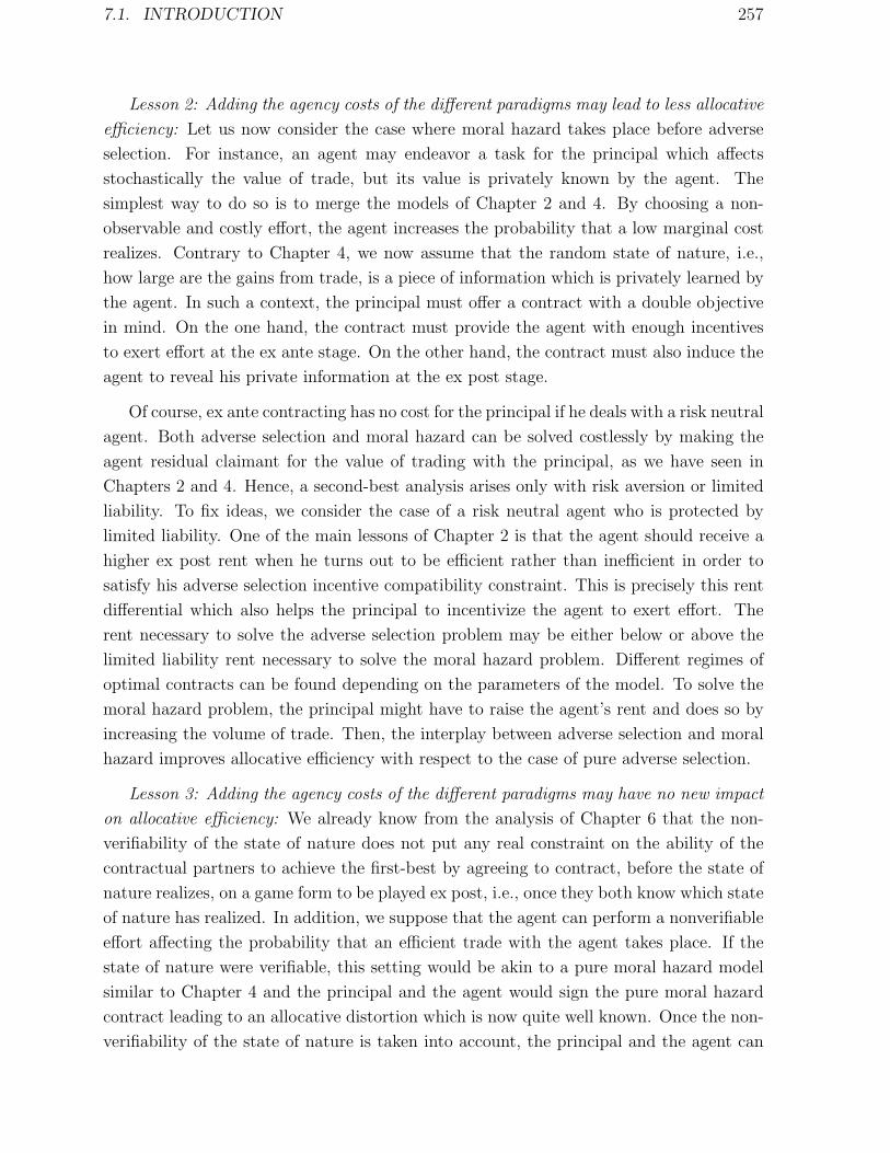
7.1. INTRODUCTION 257
Lesson 2: Adding the agency costs of the different paradigms may lead to less allocative
efficiency: Let us now consider the case where moral hazard takes place before adverse
selection. For instance, an agent may endeavor a task for the principal which affects
stochastically the value of trade, but its value is privately known by the agent. The
simplest way to do so is to merge the models of Chapter 2 and 4. By choosing a non-
observable and costly effort, the agent increases the probability that a low marginal cost
realizes. Contrary to Chapter 4, we now assume that the random state of nature, i.e.,
how large are the gains from trade, is a piece of information which is privately learned by
the agent. In such a context, the principal must offer a contract with a double objective
in mind. On the one hand, the contract must provide the agent with enough incentives
to exert effort at the ex ante stage. On the other hand, the contract must also induce the
agent to reveal his private information at the ex post stage.
Of course, ex ante contracting has no cost for the principal if he deals with a risk neutral
agent. Both adverse selection and moral hazard can be solved costlessly by making the
agent residual claimant for the value of trading with the principal, as we have seen in
Chapters 2 and 4. Hence, a second-best analysis arises only with risk aversion or limited
liability. To fix ideas, we consider the case of a risk neutral agent who is protected by
limited liability. One of the main lessons of Chapter 2 is that the agent should receive a
higher ex post rent when he turns out to be efficient rather than inefficient in order to
satisfy his adverse selection incentive compatibility constraint. This is precisely this rent
differential which also helps the principal to incentivize the agent to exert effort. The
rent necessary to solve the adverse selection problem may be either below or above the
limited liability rent necessary to solve the moral hazard problem. Different regimes of
optimal contracts can be found depending on the parameters of the model. To solve the
moral hazard problem, the principal might have to raise the agent’s rent and does so by
increasing the volume of trade. Then, the interplay between adverse selection and moral
hazard improves allocative efficiency with respect to the case of pure adverse selection.
Lesson 3: Adding the agency costs of the different paradigms may have no new impact
on allocative efficiency: We already know from the analysis of Chapter 6 that the non-
verifiability of the state of nature does not put any real constraint on the ability of the
contractual partners to achieve the first-best by agreeing to contract, before the state of
nature realizes, on a game form to be played ex post, i.e., once they both know which state
of nature has realized. In addition, we suppose that the agent can perform a nonverifiable
effort affecting the probability that an efficient trade with the agent takes place. If the
state of nature were verifiable, this setting would be akin to a pure moral hazard model
similar to Chapter 4 and the principal and the agent would sign the pure moral hazard
contract leading to an allocative distortion which is now quite well known. Once the non-
verifiability of the state of nature is taken into account, the principal and the agent can

258 CHAPTER 7. MIXED MODELS
agree, on top of this moral hazard contract, on a game form solving the non-verifiability
constraint ex post, just as in Chapter 6. We are then back to a standard pure moral
hazard problem.
In Section 7.2, we first analyze the case of adverse selection taking place before moral
hazard. With an example, we show that solving the moral hazard problem exacerbates the
allocative distortions due to adverse selection. This section also provides a version of the
Revelation Principle generalizing its applicability to models with both adverse selection
and moral hazard. Lastly, we analyze “false moral hazard problems” where the moral
hazard and the adverse selection unknowns are blend together in a deterministic way into
a single observable available for contracting. These models end up being pure adverse
selection models. They have been extensively used in the regulation and in the optimal
taxation literatures. In Section 7.3, we change the timing above and focus on models
where moral hazard takes place before adverse selection. We show that those models tend
to reduce allocative efficiency with respect to the case of pure adverse selection. Finally,
Section 7.4 analyzes the case of moral hazard followed by the nonverifiabilty of the state of
nature. We show there that non-verifiability does not put a real constraint on contracting.
7.2 Adverse Selection Followed by Moral Hazard
In the standard moral hazard framework of Chapter 3, it was first assumed that the
agent had no private information of his own. In insurance markets, insurees have often
some prior information on how risky they are before exerting any effort to prevent this
risk. Similarly, in credit markets, a borrower may know the average return of his project
before exerting any effort and sharing the resulting profits with a lender. Those examples
illustrate how frequent the interwining of adverse selection and moral hazard is. A general
formulation of these mixed models where adverse selection takes place before moral hazard
would be cumbersome to present. However, a few dimensions of the analysis can already
be singled out by studying some examples. To simplify the analysis, we start with the
case where adverse selection takes place before moral hazard.
7.2.1 Random Surplus and Screening
In the pure adverse selection framework of Chapter 2, the principal was able to verify
and contract on all the agent’s actions. Of course, when moral hazard also occurs, this
complete contractibility is no longer possible: some actions of the agent are, by definition,
under his own control only.
Consider a situation where moral hazard affects the random benefit that the principal

7.2. ADVERSE SELECTION FOLLOWED BY MORAL HAZARD 259
draws from his relationship with the agent. In the mixed model we analyze below, the
principal has already at his disposal a screening device to start with. The random benefit
S(q) he gets from dealing with the agent depends indeed on an observable, the agent’s
production q, which can be used to screen the agent’s type.
Let us thus assume that, with probability π(e) (resp. 1−π(e)) the benefit of production
obtained by the principal is Sh(q) (resp. Sl(q)) with Sh(q) > Sl(q) where, the moral hazard
variable e belongs to {0, 1}. Of course, we assume that Si(·), for i = h, l, is increasing and
strictly concave (S ′i(·) > 0 and S ′′i (·) < 0) and satisfies the Inada condition S ′i(0) = ∞. To
motivate this random surplus model, one can think of effort as improving the quality of the
product sold by the agent to the principal. Of course, exerting effort costs a non-monetary
disutility ψ(e) to the agent with, as always, the normalization ψ(0) = 0 and ψ(1) = ψ.
Moreover, the agent produces at a constant marginal cost θ. As usual, we assume that θ
belongs to Θ = {θ, θ} with respective probabilities ν and 1 − ν. For simplicity, we also
assume that the agent is risk neutral and protected by limited liability.
In this framework, the principal has two observables to screen the agent’s efficiency
parameter and we are, in fact, in a special case of the multi-output framework studied in
Section 2.11. These two observables are first, whether the good sold has a high or a low
quality and second, the amount of this good which is actually produced.
The timing of the contractual game with adverse selection being followed by moral
hazard is as in Figure 7.1:
- time
t = 0 t = 1 t = 2 t = 3
? ? ? ?
θ is realizedOnly A
learns θ
P offersa contract {t(q)}
to A
A accepts
or refusesthe contract
A exertsan effort echooses
an output qand receives t(q)
Figure 7.1: Timing of the Contractual Game
with Adverse Selection Followed by Moral Hazard.
Typically, a direct revelation mechanism is thus a menu of triplets {(th(θ), tl(θ), q(θ))}θ∈Θ
stipulating the transfers th and tl made to the agent depending on the quality of the good
and an output q as functions of the agent’s report on his type, θ.3 Moreover, we assume
3For the time being, we leave unanswered the question of whether the Revelation Principle applies inour framework and refer to Section 7.2.2 below for a formal proof that it does.

260 CHAPTER 7. MIXED MODELS
that contracting takes place at the interim stage, i.e., after the agent has learned his
private information, but before the quality of the good realizes.4 In what follows, we
also assume that the principal finds extremely valuable to always induce a high level of
effort from both types of agent.5 Using our usual notations, the efficient agent’s adverse
selection incentive constraint writes then as:
U = π1th + (1− π1)tl − θq − ψ ≥ maxe∈{0,1}
π(e)th + (1− π(e))tl − θq − ψ(e), (7.1)
with, in addition, the moral hazard incentive constraint
th − tl ≥ψ
∆π, (7.2)
so that the efficient agent exerts a positive effort.
Similarly the inefficient agent’s adverse selection incentive constraint becomes:
U = π1th + (1− π1)tl − θq − ψ ≥ maxe∈{0,1}
π(e)th + (1− π(e))tl − θq − ψ(e), (7.3)
and his moral hazard incentive constraint is:
th − tl ≥ ψ
∆π. (7.4)
Since contracting takes place at the interim stage, the agent’s participation constraints
write respectively as:
U ≥ 0, (7.5)
U ≥ 0. (7.6)
Finally, the following limited liability constraints must be satisfied. For the efficient
type:
th − θq ≥ 0, (7.7)
tl − θq ≥ 0; (7.8)
and for the inefficient type:
th − θq ≥ 0, (7.9)
tl − θq ≥ 0. (7.10)4Note that the agent must decide how much to produce before he knows whether his good will be
a good or a bad match with the agent. Transfers are instead delayed until the quality of the good islearned.
5Hence our focus is not on determining the conditions ensuring that the high effort level is second-bestoptimal.

7.2. ADVERSE SELECTION FOLLOWED BY MORAL HAZARD 261
The number of constraints is huge and our first goal should be to get rid of some of
them. A preliminary remark is useful to simplify significantly this problem. Indeed, note
that both types must be given the same transfer differential th − tl to exert effort at a
minimal cost for the principal, namely th − tl = th − tl = ψ∆π
. Hence, the right-hand sides
of both incentive constraints (7.1) and (7.3) can be simplified to yield respectively:
U = ul +π0ψ
∆π≥ ul + ∆θq +
π0ψ
∆π, (7.11)
and
U = ul +π0ψ
∆π≥ ul −∆θq +
π0ψ
∆π, (7.12)
where ul = th − θq and ul = tl − θq must remain positive by (7.7) and (7.10).
We let the reader check that the only relevant constraints are the adverse selection
incentive compatibility constraint of an efficient type (7.11) and the limited liability con-
straint of the inefficient type (7.10). The principal’s problem writes thus as:
(P ) : max{(q,ul);(q,ul)}
ν(π1Sh(q) + (1− π1)Sl(q)− θq − ul −
π1
∆πψ
)
+(1− ν)
(π1Sh(q) + (1− π1)Sl(q)− θq − ul − π1ψ
∆π
)
subject to (7.10) and (7.11).
This optimization leads immediately to ul = ∆θq + ul and ul = 0. Hence, we can
compute the rent of each type of agent respectively as
U = ∆θq +π0ψ
∆π, (7.13)
and
U =π0ψ
∆π. (7.14)
The reader will have recognized that those rents are precisely those obtained under
pure adverse selection (∆θq and 0 respectively, as in Chapter 2) added up with the limited
liability rent obtained under pure moral hazard (π0ψ∆π
, as in Chapter 4). In this simple
model with a risk neutral agent protected by limited liability constraints, the agent’s rent
coming from the mixed model is simply obtained by adding up the rents due to adverse
selection and moral hazard.
Solving for the optimal contract, the optimal outputs are obtained by equating ex-
pected marginal benefits and marginal virtual costs. For the efficient type, we find no

262 CHAPTER 7. MIXED MODELS
output distortion as in a pure adverse selection model. Indeed, we have qSB = q∗ where
the first-best production is defined by:
π1S′h(q
SB) + (1− π1)S′l(q
SB) = θ. (7.15)
For the inefficient type, we have instead:
π1S′h(q
SB) + (1− π1)S′(qSB) = θ +
ν
1− ν∆θ. (7.16)
The production of the inefficient type is distorted downwards below the first-best q∗
given by π1S′h(q
∗) + (1 − π1)S′l(q
∗) = θ. As in the case of pure adverse selection, this
downward distortion helps to reduce the agent’s information rent coming from his private
information on θ.6
The reader might think that adding moral hazard in this model has no allocative
impact on the distortion due to adverse selection which is exactly the same as if effort
was observable. This is not completely true. Indeed, the output qSB is only the solution
as long as shut-down of the least efficient type is not optimal, i.e., as long as the expected
surplus that the inefficient type generates is greater than the expected rent given up to
both types. This leads to the condition:
(1− ν)(π1Sh(q
SB) + (1− π1)Sl(qSB)− θqSB
)︸ ︷︷ ︸Expected Surplus with a θ-Type
− ν∆θqSB︸ ︷︷ ︸AdverseSelection
Rent of theθ-Type.
− π0ψ
∆π︸︷︷︸LimitedLiability
Rentof both Types
> 0.
With this condition, we see the role played by moral hazard in hardening the adverse
selection problem. Inducing effort requires to give up a limited liability rent to the ineffi-
cient type. This rent plays exactly the same role as a fixed cost in a pure adverse selection
framework (see Section 2.7.3) and it makes the shut-down of the least efficient type more
valuable for the principal.
In this particular example, we can thus conclude that moral hazard hardens the adverse
selection incentive problem. We state this as a general (but rather imprecise) proposition.
Proposition 7.1 : In mixed models with adverse selection before moral hazard, pre-
venting moral hazard hardens the adverse selection problem and allocative distortions are
greater than in a pure adverse selection setting.
6Note that the Inada condition ensures that qSB remains always positive.

7.2. ADVERSE SELECTION FOLLOWED BY MORAL HAZARD 263
Laffont (1995) analyzes a related model of environmental regulation where Sl(q) =
Sh(q) − d(q) and d(q) is an environmental damage. The added complexity of his model
comes from the fact that the disutility of effort depends on the level of production.
7.2.2 The Extended Revelation Principle
In Section 7.2.1, we have studied a simple example, assuming a priori that the Revelation
Principle holds in this context with both adverse selection and moral hazard. We prove
now this principle, still using for pedagogical purposes the basic structure of the model
of Section 7.2.1. The framework is nevertheless slightly more general since we allow now
the probability of having a high quality good to be a function of both the agent’s effort e
and his type θ. This added complexity turns out to be a useful intermediate step before
analyzing the more complex model of the insurance market covered in Section 7.2.3.
Just as in Section 2.10, let us first consider a general mechanism in this context. As
usual, a mechanism stipulates a message space M and an outcome function. Since the
quality of the good is observed, a mechanism is a triplet {th(m), tl(m), q(m)} stipulating
a transfer for each quality and an output level, as functions of the agent’s message m
which belongs to M.
Our goal is to show a Revelation Principle in such a context and to do so, we must first
describe the agent’s behavior in front of any such mechanism. This description is more
complex than in Chapter 2. Indeed, given his type, the agent must now choose not only
a message to be sent to the principal but also, given this message, what is the best effort
that he should exert. Denoting by m∗(θ) and e∗(θ) these optimal message and effort,7 we
have:
(m∗(θ), e∗(θ)) ∈ arg max(m,e)
π(θ, e)th(m) + (1− π(θ, e))tl(m)− θq(m)− ψ(e)
for all θ in Θ, e in {0, 1}, and m in M. (7.17)
Rewriting (7.17), we find:
π(θ, e∗(θ))th(m∗(θ)) + (1− π(θ, e∗(θ)))tl(m∗(θ))− θq(m∗(θ))− ψ(e∗(θ))
≥ π(θ, e)th(m) + (1− π(θ, e))tl(m)− θq(m)− ψ(e)
for all θ in Θ, in e in {0, 1} and m in M. (7.18)
Just as in Section 2.10, let us construct a direct revelation mechanism {th(θ), tl(θ), q(θ)}as follows th(θ) = t(m∗(θ)), tl(θ) = tl(m
∗(θ)) and q(θ) = q(m∗(θ)) for all θ in Θ. We can
now state our version of the Revelation Principle.7These optimal message and effort may not be unique. The Revelation Principle below holds for any
possible selection within these optimal choices.

264 CHAPTER 7. MIXED MODELS
Proposition 7.2 : There is no loss of generality in restricting the principal to offer a
truthful direct revelation mechanism {th(θ), tl(θ), q(θ)}θ∈Θ and to recommend a choice of
effort e∗(θ). With such a mechanism, the agent truthfully reveals his type to the principal
and obeys to his recommendation on the choice of effort.
Proof: The proof is straightforward and follows almost the same path as that of Propo-
sition 2.2.
Using (7.18) and the definition of the direct revelation mechanism {th(θ), tl(θ), q(θ)}associated with any mechanism {th(m), tl(m), q(m)}, we have from (7.18):
π(θ, e∗(θ))th(θ) + (1− π(θ, e∗(θ)))tl(θ)− θq(θ)− ψ(e∗(θ))
= π(θ, e∗(θ))th(m∗(θ)) + (1− π(θ, e∗(θ)))tl(m∗(θ))− θq(m∗(θ))− ψ(e∗(θ))
≥ π(θ, e)th(m) + (1− π(θ, e))tl(m)− θq(m)− ψ(e)
for all θ in Θ, e in {0, 1} and m in M. (7.19)
This latter inequality being true for all m it is in particular true for m = m∗(θ) for all
θ in Θ. Hence, we have:
π(θ, e∗(θ))th(θ) + (1− π(θ, e∗(θ)))tl(θ)− θq(θ)− ψ(e∗(θ))
≥ π(θ, e)tl(θ) + (1− π(θ, e))tl(θ)− θq(θ)− ψ(e),
for all pairs (θ, θ) in Θ2, and e in {0, 1}. (7.20)
This latter constraint means that the agent with type θ prefers to reveal his type to
the principal and obey to his recommendation on what should be the level of effort.
The Revelation Principle that we have just proved above has the same flavor as in a
pure adverse selection framework. The logic is similar: the principal can always replicate
the agent’s choices by incorporating the agent’s optimal message strategy into the initial
contract he offers. However, on top of requesting that the agent sends a truthful message
on his type, the principal also recommends now that the agent chooses a particular level
of effort.
Myerson (1982) developed in a more abstract setting the extended Revelation
Principle above. He used the expression “obedience” to characterize the fact that the
agent must follow the principal’s instructions on his choice of effort.
Remark: Instead of insisting on the principal recommending a choice of effort to the
agent, one could view this choice as being completely delegated and incorporated into the
adverse selection problem in a way that affects the different parties’ utility functions. To

7.2. ADVERSE SELECTION FOLLOWED BY MORAL HAZARD 265
see more precisely this point, let us define the agent’s indirect utility function U I(·) as:
U I(θ, q, th, tl) = maxe∈{0,1}
π(θ, e)th + (1− π(θ, e))tl − θq − ψ(e). (7.21)
The Revelation Principle can be directly applied at this stage to get the following pure
adverse selection incentive compatibility constraints:
U I(θ, q(θ), th(θ), tl(θ)) ≥ U I(θ, q(θ), th(θ), tl(θ)), for all (θ, θ) in Θ2. (7.22)
The difficulty for the modeler comes then from the fact that those incentive compat-
ibility constraints may not be as easily ordered as those of the pure adverse selection
models of Chapters 2 and 3. The indirect utility function U I(·) can indeed fail to satisfy
the Spence-Mirrlees property even in highly structured settings.
7.2.3 Insurance Contracts with Adverse Selection and MoralHazard Simultaneously
Insurance contracts are good examples of contracts designed to solve simultaneously an
adverse selection problem, how risky the agent is, and a moral hazard problem, how to
induce enough safety care from the agent. We have already touched on the analysis of
each of those two problems separately in Chapters 3 and 4. This section is aimed at
explaining how those two problems interact.
Remark: In view of the analysis of Section 7.2.1, with an insurance contract, the principal
has now only two instruments, namely a transfer whether an accident occurs or not,
to perform two tasks: incentivizing the agent to exert effort and inducing information
revelation. This creates much of the complexity of this kind of models.
Let us thus assume, that a monopoly insurer, the principal, offers an insurance contract
to agents having an initial wealth w. Agents differ ex ante according to their risk type θ.
To make things simpler, we assume that for each agent θ belongs to Θ = {θ, θ} and that
those types are independently drawn between agents with respective probabilities8 1− ν
and ν. θ (resp. θ) corresponds to a high (resp. low) risk for all levels of the moral hazard
variable e. By exerting an effort e, an agent with type θ increases his probability π(θ, e)
of not having an accident. We have thus πθ(θ, e) < 0 and πe(θ, e) > 0 for all pairs (θ, e).
Of course, the agent suffers from a disutility ψ(e) when exerting an effort. As usual, we
assume that effort belongs to {0, 1} with ψ(1) = ψ and ψ(0) = 0.
The insurance company requests from the agent a payment tn when no accident occurs
and gives a transfer ta in case of an accident. Its objective function is thus V = π(θ, e)tn−8Note that θ which refers to the “good” type has now probability 1− ν.


7.2. ADVERSE SELECTION FOLLOWED BY MORAL HAZARD 267
Truthful revelation is obtained when the following adverse selection incentive con-
straints are satisfied: For the high risk agent,
U ≥ maxe∈{0,1}
π(θ, e)u(w − tn) + (1− π(θ, e))u(w − d + ta)− ψ(e); (7.30)
and for the low risk agent,
U ≥ maxe∈{0,1}
π(θ, e)u(w − tn) + (1− π(θ, e))u(w − d + ta)− ψ(e). (7.31)
Remark: The complexity of those latter two incentive constraints already shows some of
the technical difficulties faced by the economist in modeling mixed environments. Indeed,
when he considers deviating along the adverse selection dimension and not telling the
truth anymore to the principal, the agent may also choose to change his supply of effort.
Even if inducing a high effort is optimal for the principal when both types tell the truth,
the mechanism may not require that an agent continues to exert this high effort if he lies
on his type. Even in this simple environment, the right-hand sides of (7.30) and (7.31)
can be hard to describe, since finding the values of these maximands requires to trace
out how an agent with a given risk attitude changes his effort supply when he chooses
different insurance contracts.
To simplify this problem, let us assume that effort increases more the probability that
no accident occurs when the agent is a high risk one than when he is a low risk. This
means that the following condition must be satisfied:
∆π(θ) < ∆π(θ). (7.32)
This condition ensures that the moral hazard incentive constraint for a high risk
type (7.28) is easier to satisfy than the one associated with a low risk one (7.29). In
this case, inducing effort from the low risk agent requires a wedge between u(w − tn)
and u(w − d + ta) which is large enough to ensure that a high risk agent also prefers
to exert a high effort even when he lies and mimics a low risk one. Indeed, we have
u(w − tn) − u(w − d + ta) ≥ ψ∆π(θ)
> ψ∆π(θ)
. This condition simplifies a lot the writing of
the high risk adverse selection incentive constraint which becomes now:
U ≥ π(θ, 1)u(w − tn) + (1− π(θ, 1)u)(w − d + ta)− ψ. (7.33)
Let us now introduce a new set of variables: ua = u(w − d + ta), un = u(w − tn),
ua = u(w − d + ta) and un = u(w − tn). These new variables will help us to describe
in a simpler way the set of relevant constraints. We denote also by h = u−1 the inverse
function of u(·). Using this changes of variables, the expected profit of the insurance

268 CHAPTER 7. MIXED MODELS
company writes as
ν(π(θ, 1)(w − h(un)) + (1− π(θ, 1))(w − d− h(ua)))
+(1− ν)(π(θ, 1)(w − h(un)) + (1− π(θ, 1))(w − d− h(ua)))
= w − ν(d(1− π(θ, 1))− π(θ, 1)h(un)− (1− π(θ, 1))h(ua))
−(1− ν)(d(1− π(θ, 1))− π(θ, 1)h(un)− (1− π(θ, 1))h(ua)).
The high risk agent’s adverse selection incentive constraint (7.33) becomes now:
π(θ, 1)un + (1− π(θ, 1))ua ≥ π(θ, 1)un + (1− π(θ, 1))ua. (7.34)
The high risk agent’s moral hazard incentive constraint is:
un − ua ≥ ψ
∆π(θ). (7.35)
The low risk agent’s moral hazard incentive constraint writes as:
un − ua ≥ψ
∆π(θ). (7.36)
Finally, the low risk agent’s participation constraint can be expressed as:
π(θ, 1)un + (1− π(θ, 1))ua − ψ ≥ U0. (7.37)
Neglecting the other constraints which will be checked only ex post, the insurance
company’s problem writes:
(P ′) : max{(ua,un);(ua,un)}
w − ν(d(1− π(θ, 1)) + π(θ, 1)h(un) + (1− π(θ, 1))h(ua)
)−(1− ν) (d(1− π(θ, 1)) + π(θ, 1)h(un) + (1− π(θ, 1))h(ua)))
subject to (7.34) to (7.37).
To solve this problem it is useful to recall the main features of the optimal contracts
found respectively in the case of pure adverse selection and pure moral hazard.
In Figure 7.2, we have represented the indifference curves of the high and low risk
agents when they are forced to exert a positive effort and this effort can be verified by a
Court of Justice.

7.2. ADVERSE SELECTION FOLLOWED BY MORAL HAZARD 269
-
6
un
ua¡¡
¡¡
¡¡
¡¡
¡¡
¡¡
¡¡
¡¡
¡¡
¡¡
¡Full insurance un = ua
AA
AA
AA
AA
AA
AA
AA
AA
AA
AA
APPPPPPPPPPPPPPPPPPPPPP
U0 = π(θ, 1)un + (1− π(θ, 1))ua − ψ
U0 = π(θ, 1)un + (1− π(θ, 1))ua − ψ
AA
AA
AA
AA
AA
AA
AA
AA
•BAS
•B∗
•AAS
•A∗
©©©*
Indifference curve of a θ-agent
Indifference curve of a θ-agent
¶¶/
¢¢
PPi
Figure 7.2: Insurance Contracts: The Case of Pure Adverse Selection
In Figure 7.2, the indifference curve of the agent with a low probability of accident
has a smaller slope than the indifference curve of an agent with a high such probability.
As we have shown in Section 3.4.8, if θ were perfectly known by the principal, the
agent would receive the full insurance contracts A∗ and B∗. Under pure adverse selection
instead, the high risk agent still receives full insurance at point AAS, but the low risk
agent receives contract BAS and is now imperfectly insured. Moving from B∗ to BAS
entails only a second-order loss on the profit made by the principal with the low risk
agent. However, it allows to reduce the information rent left to the high risk agent to the
first-order.

270 CHAPTER 7. MIXED MODELS
-
6
¡¡
¡¡
¡¡
¡¡
¡¡
¡¡
¡¡
¡¡
¡¡
¡¡
¡¡¡
Full insurance un = ua
¡¡
¡¡
¡¡
¡¡
¡¡
¡¡
¡¡
¡¡
¡¡
¡¡
¡¡
¡¡
¡¡
¡¡
¡¡
¡¡
¡¡un = ua + ψ
∆π(θ)
un = ua + ψ∆π(θ)
un
ua
U0 = maxe∈{0,1}
π(θ, e)un + (1− π(θ, e))ua − ψ(e)
U0 = maxe∈{0,1}
π(θ, e)un + (1− π(θ, e))ua − ψ(e)
AAAAAAAAAAEEEEEEEEEEEEE
•AMH
Incentive constraint of a θ-agent un = ua +ψ
∆π(θ)CCCW Incentive constraint of a θ-agent un = ua +
ψ
∆π(θ)?
»»»9
Indifference curve of a θ-agent³³)
Indifference curve of a θ-agent³³)
@@
@@
@@
@@
@@
@@
@@
@
XXXXXXXXXXXXXXXXXXXXXX
AAAAAAAAAEEEEEEEEEEEEEE
•uMHn
uMHn
uMHa uMH
a
³³³³1
´´
´3
BMHXXXX@
@@
@@
@@
@@
@@
@@
@@
Figure 7.3: Insurance Contracts: The Case of Pure Moral Hazard.
Let us now turn to the case of pure moral hazard where effort is non-observable but
the agent’s type is perfectly known to the insurance company. The indifference curves
of the different types have now a kink where the agent is indifferent between exerting
effort or not. Note that the assumption π(θ, 1) > π(θ, 0) for each type θ implies that
the indifference curve of each type has a smaller slope (in absolute value) when the agent
exerts a positive effort than not. Moreover, when π(θ, 0) > π(θ, 1), the indifference curves
of the two different types can only cross each other once. This single-crossing property will
play the same role as the Spence-Mirrlees condition in pure adverse selection problems. It
will help to classify the agent’s type by determining which type should attract the other
one when there will be also asymmetric information on θ. The analysis of Chapter 4 has
shown us that the insurance company would like to offer a contract AMH or BMH to the
agent depending on his observable type. Each of these contracts is lying on an indifference
curve, where, a given type of the agent is exactly indifferent between exerting effort or
not. Of course, these contracts are above the 450 line to induce effort. Therefore, they
provide only partial insurance to the agent whatever his type. See Figure 7.3.
Under pure moral hazard, we could replicate the analysis of Chapter 4, taking into
account that an agent with type θ has a non-zero reservation utility given by U0 to show

7.2. ADVERSE SELECTION FOLLOWED BY MORAL HAZARD 271
that point BMH corresponds to the ex post utility levels uMHn = U0 + ψ + (1−π(θ,1))ψ
∆π(θ)
and uMHa = U0 + ψ − π(θ,1)ψ
∆π(θ). Similarly, taking into account that a θ-agent has a non-
zero reservation utility given by U0, point AMH corresponds to the ex post utility levels
uMHn = U0 + ψ + (1−π(θ,1))ψ
∆π(θ)and uMH
a = U0 + ψ − π(θ,1)ψ
∆π(θ).
Let us now consider the more complex case entailing both moral hazard and adverse
selection. Graphically, we see that the menu of contracts (AMH , BMH) is no longer incen-
tive compatible. Following the logic of the case with pure adverse selection, the high risk
agent would like to take also contract BMH to increase his expected utility. Graphically,
the new level of utility which can be achieved is obtained by moving up the indifference
curve of a θ-agent in the north-east direction until it reaches point BMH .
More formally, the high risk agent wants to mimic the low risk one and exert an effort
when:
π(θ, 1)uMHn + (1− π(θ, 1))uMH
a − ψ = U0 −(π(θ, 1)− π(θ, 1))ψ
∆π(θ)
> π(θ, 1)uMHn + (1− π(θ, 1))uMH
a − ψ = U0.
This latter inequality holds when:
U0 − U0 = (π(θ, 1)− π(θ, 1))(u(w)− u(w − d)) >(π(θ, 1)− π(θ, 1))ψ
∆π(θ)(7.38)
which is true when assumption (7.27) is made.
To prevent the high risk agent from lying, the principal offers the pair of contracts
(ASB, BSB) described in Figure 7.4 below. Following the logic of the model with pure ad-
verse selection, the contract BSB offered to the low risk agent entails more risk than under
pure moral hazard to reduce the costly information rent of the high risk type. Graphi-
cally, the indifference curve of a θ-agent crosses now the indifference curve of a θ-agent at
a point BSB on the north-west of point BMH . The high risk agent is indifferent between
contracts ASB and BSB and the low risk agent strictly prefers BSB to ASB. Contract
BSB entails imperfect insurance to induce this type to exert an effort. It corresponds to
an expected utility greater than U0 to reward the high risk agent for having revealed his
information. Importantly, contrary to the case of pure adverse selection, by moving from
BMH to BSB, the principal no longer suffers from a second-order loss in profit, but now
from a first-order loss. This is because, contract BMH no longer maximizes the principal’s
expected profit because of moral hazard.

272 CHAPTER 7. MIXED MODELS
-
Full insurance un = ua
¡¡
¡¡
¡¡
¡¡
¡¡
¡¡
¡¡
¡¡
¡¡
¡¡
¡¡
¡¡
¡¡
¡¡
¡¡
¡¡
¡¡
ua¡¡
¡¡
¡¡
¡¡
¡¡
¡¡
¡¡
¡¡
¡¡
¡¡
¡¡
¡
6
un
@@
@@
@@
@@
@@
BBBBBBBBBBBBBBBB
@@
@@
@@
@@
@@
BBBBBBBBBBBBBBBBB
hhhhhhhhh@
@@
@@
@@
@@
@@
@@@
••
• • •BMHBAS
BSB
¡¡
¡¡
¡¡¡
AMHASB
Incentive constraint of a θ-agent un = ua +ψ
∆π(θ)AAU
Incentive contraint of a θ-agent un = ua +ψ
∆π(θ)CCW
Indifference curve of a θ-agent
U0 = maxe
π(θ, e)un + (1− π(θ, e))ua − ψ(e)¤¤²
Indifference curve of a θ-agent
U = maxe∈{0,1}
π(θ, e)un + (1− π(θ, e))ua − ψ(e)
PPPPi
Figure 7.4: Insurance Contracts: Adverse Selection and Moral Hazard.
BSB lies strictly above the low risk agent’s moral hazard incentive constraint but is affected
by moral hazard. Because of moral hazard, the high risk agent must bear some risk. This
risk affects the cost of his information rent from the principal’s point of view. This in
turn has an impact on the risk borne by the low risk agent to reduce this rent.
To see precisely how, note first that the participation constraint (7.26) is slack. Second
the adverse selection incentive compatibility constraint (7.33), the moral hazard incentive
constraint (7.36) and the participation constraint of the low risk agent are all binding at
the solution to (P ). This yields the following expressions of the second-best utilities of
each agent in each state of nature:
un(∆u) = U0 + ψ + (1− π(θ, 1))∆u (7.39)
ua(∆u) = U0 + ψ − π(θ, 1)∆u (7.40)
un(∆u) = U0 + ψ + (1− π(θ, 1))ψ
∆π(θ)− (
π(θ, 1)− π(θ, 1))∆u (7.41)

7.2. ADVERSE SELECTION FOLLOWED BY MORAL HAZARD 273
ua(∆u) = U0 + ψ − π(θ, 1)ψ
∆π(θ)− (
π(θ, 1)− π(θ, 1))∆u, (7.42)
where we make explicit the dependence of those variables on ∆u = un−ua the risk borne
by the low risk agent.
Inserting these expressions into the principal’s objective function yields a new problem:
(P ′) : max{∆u}
w − ν(d(1− π(θ, 1)) + π(θ, 1)h(un(∆u)) + (1− π(θ, 1))h(ua(∆u))
)−ν (d(1− π(θ, 1)) + π(θ, 1)h(un(∆u)) + (1− π(θ, 1))h(ua(∆u)))
subject to
∆u ≥ ψ
∆π(θ), (7.43)
where (7.43) is the low risk agent’s moral hazard incentive constraint.
Assuming that the latter constraint is slack at the optimum and optimizing with
respect to ∆u yields the following first-order condition which implicitly defines ∆uSB:
h′(uSBn )− h′(uSB
a ) =
(ν
1− ν
)(π(θ, 1)− π(θ, 1))
π(θ, 1)(1− π(θ, 1)
(π(θ, 1)h′(uSB
n ) + (1− π(θ, 1))h′(uSBa )
).
(7.44)
Since π(θ, 1) > π(θ, 1), the right-hand side above is positive and we conclude that
uSBn − uSB
a = ∆uSB > 0. Hence, the high risk agent must now bear some risk contrary to
the case of pure adverse selection.
We let the reader check that a sufficient condition to ensure that (7.43) is slack is that
the payoffs in the case of pure moral hazard, namely uMHn , uMH
a , uMHn and uMH
a are such
that:
h′(uMHn )− h′(uMH
a ) <
(ν
1− ν
)(π(θ, 1)− π(θ, 1))
π(θ, 1)(1− π(θ, 1))
(π(θ, 1)h′(uMH
n ) + (1− π(θ, 1))h′(uMHa )
).
(7.45)
Note that, when h′(·) is convex,9 Jensen’s inequality implies that the bracketed term
on the right-hand side of (7.44) is greater than h′(π(θ, 1)uSB
n + (1− π(θ, 1))uSBa
)=
h′(U0 + ψ − (π(θ, 1)− π(θ, 1))∆uSB
). Hence, we have
h′(uSBn )− h′(uSB
a ) >
(ν
1− ν
)(π(θ, 1)− π(θ, 1))
π(θ, 1)(1− π(θ, 1))h′
(U0 + ψ − (π(θ, 1)− π(θ, 1))∆uSB
).
(7.46)
9We let the reader check that this convexity property is ensured when pu(x) < 3ru(x) where pu(·) andru(·) are respectively the coefficients of prudence and risk aversion of the agent. The reader will checkthat this latter condition is, for instance, satisfied when u(·) has constant relative risk aversion.

274 CHAPTER 7. MIXED MODELS
Using the same techniques as those in Section 3.4.8, one can check that, with pure
adverse selection, the insurance company would choose to let the low risk agent bear a
positive risk ∆uAS = uASn − uAS
a such that:
h′(uASn )− h′(uAS
a ) =
(ν
1− ν
)(π(θ, 1)− π(θ, 1))
π(θ, 1)(1− π(θ, 1))h′
(U0 + ψ − (π(θ, 1)− π(θ, 1))∆uAS
),
(7.47)
where uASn = U0 + ψ + (1− π(θ, 1))∆uAS and uAS
a = U0 + ψ − π(θ, 1)∆uAS.
Under pure adverse selection, the principal’s objective function is concave with respect
to ∆u, at least when ∆θ is small enough. Using (7.46) and (7.47), it is thus immediate to
conclude that ∆uSB > ∆uAS. With adverse selection and moral hazard, the amount of
risk borne by the low risk agent is greater than with pure adverse selection. The intuition
behind this result is the following: The high risk agent must bear some risk to exert an
effort as it can be easily seen by comparing uSBn and uSB
a . This randomness of the high
risk agent’s payoff in each state of nature increases the marginal cost his information rent
when h′(·) is convex. Hence, reducing this rent calls for increasing the risk borne by the
low risk agent even more than under pure adverse selection. Point BSB lies on the north-
west of BAS on an indifference curve of the low risk agent corresponding to his expected
utility without any insurance U0.
Putting together ours findings here and those of Section 7.2.1, we can finally conclude
again that the agency costs of adverse selection and moral hazard are not simply added
one to the other as in Proposition 7.1 but strongly reinforce each other.
7.2.4 Models with “False Moral Hazard”
Another important class of mixed models entails actually no randomness at all in the
benefit obtained by the principal when dealing with the agent. The link between effort,
types and the contractual variable available to the principal is completely deterministic.
The difficulty of such models comes now from the fact that the observation of this vari-
able does not allow the principal to perfectly disentangle the type of the agent and his
level of effort. Typically, q being the observable and Q(·) being a deterministic mapping
between type and effort pairs into observables, we have q = Q(θ, e). Hence, given a target
value of q which can be imposed by the principal and given the agent’s type, effort is
completely determined by e = E(θ, q), where E(·) is implicitly defined by the identity
q = Q(θ, E(θ, q)) for all θ in Θ and all q.
Those models can be classified under the name of “false moral hazard” since the agent
has no real freedom in choosing his effort level when he has chosen how much to produce.
This lack of freedom makes the analysis of those models closely related to that of models

7.2. ADVERSE SELECTION FOLLOWED BY MORAL HAZARD 275
with pure adverse selection seen in Chapter 2. To illustrate those “false moral hazard”
models, we present two models of procurement and optimal taxation which have been
extensively used in the literature.
Example 1: The Procurement Model
Let us assume that the principal requests from the agent only one unit of good yielding
a gross surplus S. The cost of producing this unit is assumed to be observable. Had we
kept the usual specification C(θ, q) = θq with θ in Θ = {θ, θ} according to the common
knowledge distribution (ν, 1−ν), the knowledge of C = C(θ, 1) would give to the principal
complete information on θ.10 To avoid this indirect finding of the efficiency parameter
θ, let us assume that the cost of producing one unit of the good is not only related
to the efficiency parameter θ, but also to the agent’s effort e in an additive manner:
C(θ, e) = θ − e. The point is that the observation of the cost C = θ − e is not enough
to infer perfectly the agent’s productivity parameter. Intuitively, an efficient agent θ can
exert an effort e−∆θ and still produce at the same cost target as a less efficient agent θ
exerting a costly effort e.
Let us denote by t the transfer received by the agent. Since cost is observable, it is
an accounting convention to have this transfer being net of cost. The principal’s profit
writes thus as V = S − t − C. The agent’s utility becomes U = t − ψ(e), where ψ(·) is
the disutility of effort which is such that ψ′ > 0, ψ′′ > 0 and ψ′′′ ≥ 0.11 Expressed only in
terms of observables, the agent’s utility can finally be written as U = t− ψ(θ − C).
The reader will have recognized a pure adverse selection model. In this context, the
Revelation Principle tells us that there is no loss of generality in restricting the principal
to offer direct revelation mechanisms {(t(θ), C(θ))}θ∈Θ which are truthtelling.
With our usual notations, the following incentive constraints have thus to be satisfied:
U = t− ψ(θ − C) ≥ t− ψ(θ − C) = U + Φ(θ − C), (7.48)
U = t− ψ(θ − C) ≥ t− ψ(θ − C) = U − Φ(θ − C), (7.49)
where Φ(e) = ψ(e)−ψ(e−∆θ) is increasing and convex in e. The participation constraints
are also:
U ≥ 0, (7.50)
U ≥ 0. (7.51)
10See Section 9.6.2 for the case where C can also be contracted upon.11The condition on the third-derivative of ψ(·) ensures that stochastic mechanisms are never optimal.
See Section 2.14.

276 CHAPTER 7. MIXED MODELS
Note that the indifference curves of both types in the space (t, C) satisfy the single-
crossing property with those of the efficient type having a smaller slope. The reader will
have recognized the Spence-Mirrlees condition which allows us to conclude that, at the
optimal contract, the relevant binding constraints are (7.48) and (7.51). The principal’s
problem writes thus as:
(P ) : max{(U,C);(U ,C)}
S − ν (C + ψ(θ − C) + U)− (1− ν)(C + ψ(θ − C) + U)
subject to (7.48) and (7.51).
Both constraints above are binding at the optimum and we have thus USB = Φ(θ −CSB) and USB = 0.
Optimizing with respect to the cost targets C and C amounts to optimize with respect
to the effort levels e and e indirectly requested respectively from an efficient type and
from an inefficient one, once one has recognized that those costs targets and efforts are
respectively linked by the relationships C = θ−e and C = θ−e. Expressing the principal’s
objective function in terms of efforts and taking into account that (7.48) and (7.51) are
both binding at the optimum, the principal’s problem becomes:
(P ′) : max{e,e}
S − ν(θ − e + ψ(e) + Φ(e))− (1− ν)(θ − e + ψ(e)).
Optimizing with respect to e and e yields:
ψ′(eSB) = 1, (7.52)
and
ψ′(eSB) = 1− ν
1− νΦ′(eSB). (7.53)
Note that under complete information, both types would be asked to exert the same
first-best level of effort e∗ such that the marginal disutility of effort equals the marginal
cost reduction, i.e., ψ′(e∗) = 1. Under asymmetric information, only the most efficient
type continues to exert this first-best level of effort. To reduce the costly information rent
of this efficient type, the effort of the less efficient one is reduced below the first-best and
eSB < e∗.
These results are not surprising in view of Chapter 2. However, the novelty comes here
from the interpretation of the model. The efficient agent being residual claimant for his
effort, we will say that he is put on a “high-powered incentive scheme” which is akin to a
fixed fee contract. The inefficient agent under-supplies effort because he is only partially
residual claimant for his effort. We will say that he is put instead on a “low-powered
incentive scheme” which is closer to a cost-plus contract.

7.2. ADVERSE SELECTION FOLLOWED BY MORAL HAZARD 277
To better understand these denominations, let us assume that the principal offers
a nonlinear contract {T (C)} with is defined over all C in [0, +∞[. This mechanism
should implement precisely the second-best allocation computed above, when the agent
finds optimal to exert effort eSB and eSB. Assuming differentiability of the schedule
T (C) at points CSB and CSB, we must have T ′(CSB) = ψ′(θ − CSB) = ψ′(eSB) and
T ′(CSB) = ψ′(θ − CSB) = ψ′(eSB).12 Identifying with (7.52) and (7.53), we find that
T ′(CSB) = 1 and T ′(CSB) < 1. This shows that only the efficient agent is given full
incentives in cost reduction. The inefficient agent gets only a function of his marginal
effort in cost reduction and thus under-provides effort.
Let us now turn to the shape of the nonlinear schedule {T (C)}. To get some ideas on
this shape, it is useful to look at Figure 7.5:
-
6
LLLLLLLLLL
•
•
C∗ CSB
Tt
C
A
B
-Nonlinear schedule T (C)
Indifference curve of aθ-agent
U = 0 = t− ψ(θ − C)´+
tSB
tSB
Indifference curve of aθ-agent
U = Φ(eSB) = t− ψ(θ − C)
©©*
@@
@@
@
Figure 7.5: Implementation through a Nonlinear Schedule T (C).
To ensure that the agent, whatever his type, chooses the second best cost target
computed by the principal, it is enough that the nonlinear transfer T (C) be tangent to
12We will see in Figure 7.5 below that this differentiability is not exactly satisfied. In this case, thefirst-order condition above is only true for the right-hand side derivative of T (C) at CSB .

278 CHAPTER 7. MIXED MODELS
each indifference curve at points A and B. We may thus define T (C) as:
T (C) =
tSB + ψ′(e∗)(C − C∗) for C ≤ C∗ = θ − e∗,ψ(θ − C) for C in [C∗, CSB],tSB + ψ′(eSB)(C − CSB) for C ≥ CSB = θ − eSB.
Remark: In the case of a continuum of types, we will see in Chapter 9 when the optimal
contract can be implemented through a menu of linear contracts.
This procurement model is due to Laffont and Tirole (1986 and 1993) who have
built a whole theory of regulation and procurement with elements of both moral hazard
and adverse selection. Interesting issues arise in the case where output is no longer zero or
one as in this model. Indeed, output can then be used as a screening variables. Depending
on the exact mapping between cost, output, effort and types, the pricing rule may or may
not be distorted under asymmetric information. When it is not, Laffont and Tirole argue
that there is a dichotomy between the pricing rule and the provision of incentives.
Example 2: The Income Taxation Model
Let us now return to the optimal redistribution model studied in Section 3.8. One weak-
ness of that model was the fact that the government was assumed to be unable to observe
the income of each agent. Standard taxation models relax this somewhat irrealistic as-
sumption. To still have a meaningful informational problem, we assume now that each
agent produces an amount q = θe when his productivity parameter is θ. θ belongs to
Θ = {θ, θ} with respective probabilities 1 − ν and ν and his effort e. Effort costs to the
agent a disutility ψ(e) with ψ′ > 0, ψ′′ > 0 and ψ′′′ ≥ 0 as before.
Normalizing the price of the production good at one, q also represents the agent’s
income which is now assumed to be observable by the government. Note the similarity of
this model with the procurement model above. Instead of being blended additively, type
and effort are now blended multiplicatively into the observable available to the principal.
When exerting effort e and paying a tax τ , the agent with productivity θ gets a utility
U = q − τ − ψ(e), or, replacing effort as a function of the agent’s type and his income,
U = q− τ −ψ(
qθ
). Again, the reader will have recognized that we are now back to a pure
adverse selection model. In this context, a taxation mechanism can be viewed as a menu
{τ , q); (τ , q)} where q is the agent’s revenue and τ is the tax. The incentive compatibility
constraints for this model write as:
U = q − τ − ψ( q
θ
)≥ q − τ − ψ
(q
θ
)= U + Φ(e), (7.54)
and
U = q − τ − ψ
(q
θ
)≥ q − τ − ψ
(q
θ
)= U − Φ(e), (7.55)

7.2. ADVERSE SELECTION FOLLOWED BY MORAL HAZARD 279
where Φ(e) = ψ(e)−ψ(e θ
θ
)is increasing and convex in e from the assumptions made on
ψ(·), (Φ′ > 0, Φ′′ > 0).
On top of these incentive constraints, a taxation scheme is feasible if it satisfies the
government budget constraint ντ + (1− ν)τ ≥ 0.13 Expressing taxes as a function of the
rents U and U and efforts e and e, this budget constraint becomes:
ν(θe− ψ(e)) + (1− ν)(θe− ψ(e)) ≥ νU + (1− ν)U. (7.56)
The government wants to maximize the social welfare function νG(U) + (1− ν)G(U),
where G(·) is increasing and concave (G′ > 0, G′′ < 0). The principal’s problem is thus:
(P ) : max{(U,e);(U ,e)}
νG(U) + (1− ν)G(U),
subject to (7.54) to (7.55).
We let the reader check that the relevant incentive constraint is, as usual, that of the
most productive type θ. Denoting by µ the multiplier of the budget constraint (7.56) and
by λ the multiplier of the incentive constraint (7.54), we can write the Lagrangean of the
problem as L(U , U, e, e) = νG(U) + (1− ν)G(U) + µ(ν(θe− ψ(e)− U))
+ (1− ν)(θe−ψ(e)−U)) + λ(U −U −Φ(e)). Optimizing with respect to U and U yields
respectively:
νG′(USB) = µν − λ, (7.57)
(1− ν)G′(USB) = µ(1− ν) + λ. (7.58)
Summing (7.57) and (7.58), we obtain:
µ = νG′(USB) + (1− ν)G′(USB) > 0, (7.59)
and thus the budget constraint (7.55) is binding. Inserting this value of µ into (7.57), we
get:
λ = ν(1− ν)(G′(USB)−G′(USB)
). (7.60)
Since USB > USB is necessary to satisfy the incentive constraint (7.54) and since G(·)is concave, we have λ > 0. Hence, the incentive constraint (7.54) is also binding.
Optimizing with respect to efforts, we immediately find that:
ψ′(eSB) = θ, (7.61)
13As in Section 3.8, we normalize public expenditure to zero without loss of generality.

280 CHAPTER 7. MIXED MODELS
and
ψ′(eSB) = θ − ν(G′(USB)−G′(USB))
νG′(USB) + (1− ν)G′(USB)Φ′(eSB). (7.62)
In the complete information framework, the government could perfectly redistribute
wealth between both groups of agents to equalize their utilities. Moreover, the government
could recommend to exert first-best efforts e∗ and e∗ such that the marginal disutility of
effort of each type equals his productivity in each state of nature, i.e., ψ′(e∗) = θ and
ψ′(e∗) = θ.
Under asymmetric information, only the most productive agent still exerts the first-
best level of effort. Inducing information revelation calls for creating a positive wedge
between the utilities of the high and the low productivity agents. Because the principal is
adverse to inequality in the distribution of utilities, this risk is socially costly. To reduce
this cost, the principal reduces the low productivity agent’s effort below its first-best value
eSB < e∗.
Interestingly, it is worth to recast these results in terms of the progressiveness or not
of the tax schedule. Indeed, as in the procurement model above, let us think of this
optimal allocation as being implemented by a nonlinear income tax {τ(q)}. When he
faces this nonlinear tax, the high (resp. low) productivity agent will respectively choose
to exert the second best level of efforts eSB and eSB such that θ− τ ′(θeSB) = ψ′(eSB) and
θ − τ ′(θeSB) = ψ′(eSB). Using (7.61) and (7.62), the marginal tax rates which concern
each type are thus τ ′(q) = 0 and τ ′(q) > 0. Hence, the high productivity agent is not
taxed at the margin. The marginal tax rate at the top of the distribution is zero. The
low productivity agent has instead a positive marginal tax rate. The optimal taxation
scheme is thus regressive at the margin, a surprising feature which has emulated much
debate in the optimal taxation literature.
The basic model above is that of Diamond (1998) who simplifies the initial
framework of Mirrlees (1971) by restricting the analysis to quasi-linear utility functions.
7.3 Moral Hazard Followed by Adverse Selection
Sometimes an agent undertakes an initial nonverifiable investment or performs an effort
before producing any output for the principal. For instance, the agent can choose a
costly technology which affects the distribution of his marginal cost of production. At
the time of choosing whether to incur the nonverifiable investment or not, the agent is
still uninformed on what will be the realization of his efficiency parameter ex post. If this

7.3. MORAL HAZARD FOLLOWED BY ADVERSE SELECTION 281
efficiency parameter is privately known, we are now in a framework where moral hazard
takes place before adverse selection.
7.3.1 The Model
We assume that the agent can change the stochastic nature of the production process by
exerting a costly effort e which again belongs to {0, 1}. The disutility of effort is as usual
normalized so that ψ(0) = 0 and ψ(1) = ψ. When exerting effort e, the agent induces a
distribution of the productivity parameter θ on Θ = {θ, θ}. With probability ν(e) (resp.
1 − ν(e)), the agent will be efficient (resp. inefficient) and we denote for the sake of
simplicity ν(1) = ν1, ν(0) = ν0 and ∆ν = ν1− ν0. To capture the fact that exerting effort
is valuable, we assume that effort increases the probability that the agent is efficient, i.e.,
∆ν > 0.
If the efficiency parameter is θ, when the agent produces an output q and receives
a transfer t from the principal, his utility writes as U = u(t − θq) − ψ(e), where u(·)is increasing and concave (u′(·) > 0, u′′(·) ≤ 0) with h = u−1 the inverse of the utility
function.14 The principal is risk neutral and has the usual utility function V = S(q)− t.
Through the contract he offers to the agent, the principal wants to control both the
agent’s effort and the agent’s incentives to tell the truth on the state of nature which
realizes ex post. The timing of the contractual game is described in Figure 7.5 below.
- time
t = 0 t = 1 t = 2 t = 3 t = 4
? ? ? ? ?
P offersa contract {t(q)}
to A
A accepts
or refusesthe contract
A exertsan effort e
θ is realizedOnly A
learns θ
A chooses qand receives t(q)
Figure 7.6: Timing of the Contractual Game
with Moral Hazard Followed by Adverse Selection.
In this mixed environment, the contract {t(q)} must not only induce effort if the
principal finds it sufficiently valuable, but it must also induce information revelation.
Applying the Revelation Principle at t = 3, there is no loss of generality in restricting the
14Note that the utility function is separable between monetary gains and effort. This is without lossof generality for what follows.
282 CHAPTER 7. MIXED MODELS
principal to offer a direct revelation mechanism {(t, q); (t, q)}. Through this contract, the
agent will be induced to reveal his private information on the state of nature θ.
Of course, this contract being signed before the realization of the state of nature, we
are in the case of ex ante contracting similar albeit more complex than that in Sections
2.12 and 4.4.
7.3.2 The Case of Risk Neutrality
To explain the new issues arising with this type of mixed models, we start by analyzing
the case of risk neutrality. We already know that the agent’s risk neutrality calls for
no allocative distortions either under pure moral hazard or under pure adverse selection.
With pure adverse selection as well as with pure moral hazard, the first-best outcome can
be implemented by letting the agent be residual claimant for the hierarchy’s profit. One
may wonder whether adding those two informational problems leads to significant new
problems even with risk neutrality.
Let us start by describing the first-best outcome. The first-best outputs equalize the
marginal benefit and the marginal cost of production so that S ′(q∗) = θ, and S ′(q∗) = θ.
Denoting by W ∗ = S(q∗)− θq∗ and W ∗ = S(q∗)− θq∗ the first-best surplus in each state
of nature, inducing effort is socially optimal whenever:
∆ν(W ∗ − W ∗) > ψ. (7.63)
We will assume that this last condition holds in what follows.
Let us now look at the case of moral hazard and adverse selection. One may wonder
if making the agent residual claimant still helps in this framework. Consider thus the
following transfer t∗ = S(q∗)− T and t∗ = S(q∗)− T where the constant T will be fixed
below.
First, we claim that the contract {(t∗, q∗); (t∗, q∗)} induces information revelation by
both types. Indeed, t∗ − θq∗ = S(q∗) − θq∗ − T > t∗ − θq∗ = S(q∗) − θq∗ − T by the
definition of q∗ and t∗ − θq∗ = S(q∗) − θq∗ − T > t∗ − θq∗ = S(q∗) − θq∗ − T by the
definition of q∗. Second, the contract {(t∗, q∗); (t∗, q∗)} also induces effort. Indeed, the
agent’s expected payoff from exerting effort is ν1W∗ + (1− ν1)W
∗− (ψ + T ). It is greater
than his expected payoff from not exerting effort which is ν0W∗ + (1− ν0)W
∗ − T when
(7.63) holds. Finally, the principal fixes the lump sum payment T to reap all ex ante
gains from trade with the agent, namely T = ν1W∗ + (1 − ν1)W
∗ − ψ. Henceforth, we
can state:
Proposition 7.3 : When moral hazard takes place before risk aversion and the agent

7.3. MORAL HAZARD FOLLOWED BY ADVERSE SELECTION 283
is risk neutral, the first-best outcome can still be achieved by making the agent residual
claimant for the hierarchy’s profit.
Note also that the contract which makes the agent residual claimant for the hierarchy’s
profit ensures the principal against any risk since S(q∗)−t∗ = S(q∗)−t∗ = T . This contract
works also perfectly well if the principal is risk averse.
7.3.3 Limited Liability and Output Inefficiency
Introducing the agent’s risk aversion or protecting the risk neutral agent with limited
liability makes the implementation of the first-best outcome obtained above no longer
optimal. To see this, let us assume that the agent is still risk neutral, but is now protected
by limited liability. Assuming that he has no asset to start with, the limited liability
constraints in the two states of nature write as:
U = t− θq ≥ 0, (7.64)
and
U = t− θq ≥ 0. (7.65)
Moreover, inducing information revelation at date 4 through a direct revelation mecha-
nism requires to satisfy the following adverse selection incentive compatibility constraints:
U ≥ U + ∆θq, (7.66)
and
U ≥ U −∆θq. (7.67)
In our mixed environment, the rents U and U must also serve to induce effort. To in-
duce effort as under complete information, the following moral hazard incentive constraint
must now be satisfied:
U − U ≥ ψ
∆ν. (7.68)
Finally, the agent accepts the contract at the ex ante stage when his ex ante partici-
pation constraint is satisfied:
ν1U + (1− ν1)U − ψ ≥ 0. (7.69)

284 CHAPTER 7. MIXED MODELS
Still focusing on the case where it is always worth inducing the agent’s effort, the
principal’s problem is thus:
(P ) : max{(U,q);(U ,q)}
ν1(S(q)− θq − U) + (1− ν1)(S(q)− θq − U),
subject to (7.64) to (7.69).
Depending on the respective importance of the moral hazard and adverse selection
problems, the optimal contract may exhibit different properties. Some of the possible
regimes of this optimal contract are summarized in the next proposition.
Proposition 7.4 : With moral hazard followed by adverse selection and with a risk neu-
tral agent protected by limited liability, the optimal contract has the following features:
• For ψ∆ν
≤ ∆θqSB(ν1), (7.65) and (7.66) are both binding. Outputs are given by
qSB = q∗ when θ realizes and qSB = qSB(ν1) < q∗ when θ realizes with:
S ′(qSB(ν1)) = θ +ν1
1− ν1
∆θ. (7.70)
• For ∆θqSB(ν1) ≤ ψ∆ν≤ ∆θq∗, (7.65), (7.66) and (7.68) are all binding.
The first-best output q∗ is still requested when θ realizes. Instead, production is
downward distorted below the first-best when θ realizes. We have qSB < q∗ with:
qSB =ψ
∆θ∆ν. (7.71)
• For ∆θq∗ < ψ∆ν
< ∆θq∗, (7.65) and (7.68) are both binding. In both states of nature
the first-best outputs are implemented.
To understand how those different regimes emerge, first, note that solving the pure
adverse selection problem requires to create a differential between the rents U and U .
This rent differential may be enough to induce effort when the corresponding disutility is
small. In this case, moral hazard has no impact and second-best distortions are completely
driven by adverse selection. As effort becomes more costly, the pure adverse selection rent
may no longer be enough to induce effort. The output when θ realizes must be distorted
upward to provide enough rent so that, ex ante, the agent wants to perform an effort.
Finally, still increasing the disutility of effort, output distortions are no longer worth to
be made and the principal prefers to maintain allocative efficiency in both states of nature
and to reward the agent sufficiently to induce his effort. The design of the contract is
then purely driven by moral hazard.

7.4. MORAL HAZARD FOLLOWED BY NON-VERIFIABILITY 285
Remark: The reader will have recognized the similarity of the analysis above with that
made in Section 3.4 when we analyzed type dependent reservation values in pure adverse
selection models. Indeed, one can view the design of incentives in this mixed model as a
two-step procedure. The first step consists for the principal in offering a reward when θ
realizes which is large enough to induce effort provision at the ex ante stage. By doing so,
the principal commits to solve the moral hazard problem. Then, the second step consists
in solving the adverse selection problem and inducing information revelation. At this ex
post stage, the principal may or may not be constrainted by his previous commitment in
extracting the agent’s private information on the state of nature which has realized.
To conclude, we stress that the main impact of the initial stage of moral hazard may
be to reduce allocative distortions and to call for higher information rents with respect to
the case of pure adverse selection.
Proposition 7.5 : Mixed models with moral hazard followed by adverse selection tend
to be characterized by less allocative distortions and higher information rents than models
with pure adverse selection.
7.4 Moral Hazard Followed by Non-verifiability
The last stage of our travel among mixed models brings us to the analysis of the case
where the agent exerts first a non-observable effort which affects the realization of the
state of nature, but this state of nature is nonverifiable even though it remains common
knowledge between the principal and the agent. The timing of the contractual game is
thus exactly the same as in Figure 7.5, except that, at date 3, the state of nature θ is
observed by both the principal and the agent.
If effort was observable, we would be in the case of models with pure non-verifiability
of the state of nature θ. The analysis we made in Chapter 6 has shown how the principal
and the agent can then agree ex ante, i.e., at date 0, on a mechanism, more precisely an
extensive form game, which ensures that the first-best outcome can be uniquely imple-
mented. An important issue is thus to know how much of this result still holds when effort
is not observable by the principal. The answer is quite unsurprising: the first-best can
generally be no longer implemented, but the non-verifiability of the state of nature does
not bring more distortion than what we find in a model with only moral hazard. In other
words, an upper bound of what can be achieved by the principal in a mixed model with
moral hazard and non-verifiability is obtained in the model with pure moral hazard where
the state of nature could be described ex ante and used to write the contract. Moreover,

286 CHAPTER 7. MIXED MODELS
this upper bound is actually achieved.
To prove this result, let us consider the pure moral hazard model of Section 4.5. Only
the agent’s effort cannot be verified. Assuming that the principal wants to induce a high
effort from a risk averse agent, we know that he must let the latter bear some risk.
Still denoting by U = t− θq and U = t− θq the rents obtained by the agent in each
state of nature, the agent’s moral hazard incentive compatibility constraint writes as:
u(U)− u(U) ≥ ψ
∆ν. (7.72)
The agent’s participation constraint is
ν1u(U) + (1− ν1)u(U)− ψ ≥ 0. (7.73)
Under pure moral hazard, the principal’s problem becomes:
max{(U,q);(U ,q)}
ν1(S(q)− θq − U) + (1− ν1)(S(q)− θq − U)
subject to (7.72) and (7.73).
Repeating the analysis of Chapter 4, we know that (7.72) and (7.73) are both binding.
This yields the following expressions of the moral hazard rents in each state of nature:
UMH = h
(ψ + (1− ν1)
ψ
∆ν
)> 0, (7.74)
and
UMH = h
(ψ − ν1
ψ
∆ν
)< 0, (7.75)
Moreover, the optimal outputs chosen by the principal in each state of nature are
equal to their first-best values: q∗ such that S ′(q∗) = θ when θ realizes and q∗ such
that S ′(q∗) = θ when θ realizes. Transfers in each state of nature are thus given by
tMH = θq∗ + UMH and tMH = θq∗ + UMH .
Let us now describe in Figure 7.7 these contracts by points AMH and BMH .

7.4. MORAL HAZARD FOLLOWED BY NON-VERIFIABILITY 287
-
6
©©©©©©©©©©©©©©©©©©©©©©©©©©©©©©©©©
©©©©©©©©©©©©©©©©©©©©©©©©©©©©©©©©©
¢¢¢¢¢¢¢¢¢¢¢¢¢¢¢¢¢¢¢¢¢¢¢¢¢¢¢¢¢
•
•
t
q
q∗
tMH
q∗
tMH
BMH
AMH
•(t2, q2)
F
E
6
UMH = t− θq
WMH = S(q)− t
CCCW
UMH = t− θqSSw
WMH = S(q)− t½
½½>
•
(t1, q1)¤¤¤¤¤
@@
@@
@@
@
@@
@@
@@
@@
@
@@
@@
@@
@@
@@
@@
@
Figure 7.7: Moral Hazard and Non-verifiability.
Let us now turn to the case where the state of nature θ is nonverifiable. We know
that signing no contract ex ante is generally a dominated outcome. Indeed, assuming
that the principal keeps all bargaining power in the ex post bargaining stage, the agent
gets zero rent in each state of nature. Anticipating this, the agent has thus no incentive
to exert effort at the ex ante stage. This is an instance of the “hold-up” problem that we
will more extensively discuss in Section 9.5.2. Signing at the ex ante stage an incentive
compatible contract implies also some allocative inefficiency with a risk averse agent as
we know from Section 2.12.2. Those inefficiencies can be avoided if the agent and the
principal agree to play a mechanism ex post where both report messages over the state
of nature. To implement the pure moral hazard outcome (AMH , BMH), we will thus have
to rely on Nash implementation which now gets all its strength.
Taking the same notations as in Chapter 6, the game form to be played in each state
of nature is as in Figure 7.8 below.

288 CHAPTER 7. MIXED MODELS
P ’s strategy
θ θ
θ (tMH , q∗) (t2, q2)A’s strategy
θ (t1, q1) (tMH , q∗)
Figure 7.8: Nash Implementation in a Mixed Model.
The conditions for Nash implementation of the outcome with pure moral hazard are
then easy to obtain.
To have a truthful Nash equilibrium in state θ, we should have:
tMH − θq∗ > t1 − θq1, (7.76)
S(q∗)− tMH > S(q2)− t2. (7.77)
Similarly, to have a truthful Nash equilibrium in state θ, we should have:
tMH − θq∗ > t2 − θq2, (7.78)
S(q∗)− tMH > S(q1)− t1. (7.79)
Finally, unique Nash implementation in both states of nature is obtained when:
tMH − θq∗ < t2 − θq2, (7.80)
and
tMH − θq∗ < t1 − θq1. (7.81)
The possible values of (t1, q1) (resp. (t2, q2)) satisfying constraints (7.76), (7.79) and
(7.81) (resp. (7.77)), (7.80) and (7.81) belong to set E (resp. F ) in Figure 7.7.
We let the reader check that those sets are non-empty and thus the moral hazard
contract (tMH , q∗) and (tMH , q∗) appended with the out-of-equilibrium punishments (t1, t2)
and (t2, q2) allows to get rid of the non-verifiability constraint.

Chapter 8
Dynamics Under Full Commitment
8.1 Introduction
Contracts are often repeated over time. Examples of such long-term relationships abound
and span all areas of contract theory. Let us just describe a few. The insurance contract of
an agent entails bonuses and maluses which link his current coverage and risk premium to
his past history of accidents. Labor contracts often still continue to reward in the future
the past performances of an agent either in monetary terms or by means of promotions.
Lastly, in many regulated sectors, regulatory contracts often stipulate the current price-
caps which apply to a given firm as a function of the past realizations of its costs.
In view of the analysis of the previous chapters, the general framework to understand
those repeated contractual relationships must be one where the principal controls sev-
eral activities performed by the agent at different points in time. In an adverse selection
setting, the reader will probably have recognized the multi-output framework of Section
2.11. Under moral hazard, the setting is akin to a multi-task model along the general
lines of Section 5.3. With respect to those general frameworks, the repeated contracting
setting has nevertheless its own peculiarities which are worth studying. Let us mention
a few: the principal and the agent’s utility functions are separable over time, the infor-
mation structures may change as time passes, lastly, the arrow of time creates a natural
asymmetry between the control of today and tomorrow relationships.
Indeed, the analysis of repeated contractual relationships raises a number of questions.
How does the repeated contractual relationships compare with the one-shot relationship
studied in previous chapters? How does the repetition of the relationship changes the
terms of the statics trade-offs? How should we model changes in information structures?
What are the benefits, if any, of long lasting relationships? Does the past history of the
agent’s performance play any role on current compensation and why is it so?
289

290 CHAPTER 8. DYNAMICS UNDER FULL COMMITMENT
To answer these questions, we remain in the general framework of this volume1 and
assume that the principal has the ability to commit to the contract he proposes to the
agent. The principal designs the rules of a game that is going to be played over time by
the agent and sticks to these rules no matter what happens during the relationship.2
Even though the information structures associated with moral hazard and adverse
selection dynamic models look somewhat different, they can be classified within three
broad categories which give rise to similar conclusions in both paradigms.
• Permanent Shocks: In an adverse selection setting, the agent’s private information on
the value of the trades that can be performed at different points of time may be constant
over time. For instance, a regulated firm has a constant technology over the whole length
of the regulated contract. A worker has a constant ability over the length of the labor
contract. An insuree has a driving ability, i.e., a probability of having an accident, which
does not change over his entire life. In such a setting, the optimal long-term contract
is straightforwardly obtained as the replica of the one-shot optimal contract described in
Chapter 2. To see that, note that, under the assumptions of separability of the principal’s
and the agent’s utility functions between today and tomorrow trades, the intertemporal
benefits of a given profile of trades and its intertemporal costs, including informational
costs, are just obtained as the discounted sum of the benefit and cost of the volumes of
trades chosen in the different periods. In each given period, the optimal trade-off between
rent extraction and efficiency is similar to that in a one-shot static relationship. The
optimal long-term contract is thus obtained as the replica of the static optimal contract.
Importantly, one way of implementing this long-term optimal contract is given by
the dynamic version of the Revelation Principle under full commitment. With a direct
mechanism, the agent is requested to reveal his type once and for all to the principal
before any trade takes place. The principal commits then to replicate the one-shot optimal
contract in each period of their relationship.3
1See Chapters 2 and 4.2In particular, commitment implies that the agents still continue to play the same game no matter what
the principal may have learned about the agent during the first rounds of contracting. This assumptionis an important one because the endogenous changes in the information structures which may arisein a repeated relationship may open the door to valuable renegotiations as time passes. Even thoughthose issues are particularly important for the understanding of enduring relationships, they are byand large beyond the scope of this volume and are relegated, by mean of an example, to Chapter 9.Note nevertheless, that, in a number of the contractual settings that we analyze in this chapter, theassumption of commitment does not represent a restriction since the optimal long-term contract turnsout to be sequentially optimal, i.e., recontracting from a given date on would not improve on what isspecified by the full commitment optimal contract.
3Even if we do not develop the corresponding analysis in the present chapter, it is worth mentioningbriefly what would be the moral hazard counterpart to this model. Let us assume that the agent isperforming a single effort in an initial period and then the random stochastic production process associatedwith this performance is replicated over several periods. It is straightforward to see that all that mattersfor the principal and the agent is the overall performance over the whole relationship. Hence, the optimal
8.1. INTRODUCTION 291
Because of these analogies between the optimal dynamic contract and a static optimal
contract, those models have sometimes been coined under the general terminology of
“false dynamics”.
• Correlated Shocks: Still in an adverse selection setting, let us now turn to the more
general case where the agent has private information on the values of trade with the
principal in each period and those values are correlated over time. For instance, the cost of
producing a good for a seller may be the sum of two components: a permanent component
linked to the production technology and a transient component linked to short-term shocks
on the price of inputs. Similarly, because of learning by doing, a worker’s ability may
change over time, but still with some correlation across periods. Those contractual settings
are interesting because the mere realizations of the first period volumes of trade convey
information on the future values of trade. The Revelation Principle still applies to those
contractual relationships if one requests the agent to report any information he learns
over the course of actions. In a direct revelation mechanism, the agent decides to report
truthfully his type to the principal in any given period, knowing that the principal uses this
information to possibly update his beliefs on the agent’s future types and may therefore
specify different continuations of the long-term contract depending on this latter report.
This effect allows us to derive dynamic incentive constraints in a simple model with two
periods and a risk neutral agent. We then show how the principal should design the
intertemporal contract by using earlier revelations of information in order to improve the
terms of the dynamic rent extraction-efficiency trade-off.
It is interesting to observe the link between those latter models and the model of
informative signals improving contracting already studied in Section 2.15. In that section,
we analyzed how the principal may benefit from exogenous signals which are correlated
with the agent’s information to improve the terms of the rent extraction-efficicency trade-
off in a static model. In dynamic relationships with correlated shocks, the past history
of reports offers an endogenous signal which is correlated with the agent’s current type.
History-dependent contracts are useful to take into account the informativeness of earlier
performances. As a corollary, the optimal long-term contract is no longer obtained as the
replica of the one-shot optimal contract.
Again, it is worth pointing out the moral hazard counterpart to this model. Let us
assume that the agent is performing a different effort at each date of his relationship
with the principal but that the random stochastic productions at each different date are
correlated. In such a framework, it is a simple corollary of the Sufficient Statistics Theorem
of Section 4.7.1 that the current performances should be used in future compensations.
contract is again akin to an optimal static contract where the stochastic returns of the agent’s effort aresimply the discounted sum of the per period profits.

292 CHAPTER 8. DYNAMICS UNDER FULL COMMITMENT
• Independent Shocks: Let us now envision a case where there is no correlation across
periods among the values of trade. For instance, an agent may be looking for insurance
against independently distributed income shocks or a seller may be subject to one-period
independent shocks on his costs. In such a model, the past history of the agent’s perfor-
mances loses any informative role on the current values of trade. It does not mean that
history plays no longer any role. Indeed, history may allow to smooth the cost of incentive
compatibility over time.
To stress this new effect, we develop a two period simple moral hazard model in the
context of an efficiency-insurance trade-off. The model is basically a twice-replica of that
of Chapter 4.4 We derive the dynamic incentive compatibility constraint and optimize the
principal’s intertemporal objective function. We show that the optimal contract exhibits a
martingale property linking current compensations with future rewards and punishments.
The source of this property comes from the desire of the principal to smooth the cost
of incentive compatibility over time. We discuss how this smoothing can be somewhat
perturbed if the agent can save part of his wealth or can end the relationship in any given
period. Then, we develop an infinitely repeated version of the model to explore issues such
that the intertemporal distribution of utilities achieved in the long run or the behavior of
the contract as the discount factor goes to one. We show that agency problems disappear
in the limit by mean of a complete diversification of the risk borne by the agent in any
given period.
Section 8.2 presents the dynamics of adverse selection models for a two period example.
We make there various assumptions on the information structure and derive some of
the conclusions stressed above. In Section 8.3, we briefly discuss the full commitment
assumptions. Section 8.4 deals with the case of moral hazard both in a two-period model
with various contractual limits but also in an infinitely repeated setting. We provide there
the basic dynamic programming methods necessary to analyze such a setting. Section 8.5
concludes by discussing an application: the insurance market.
8.2 Adverse Selection
Consider the twice repetition of the model in Chapter 2 where we can make various
assumptions on the information structure and, in particular, on how it evolves over time.
4Similarly, smoothing the cost of the incentive compatibility constraint would also be present in anadverse selection framework with ex ante contracting and risk-aversion on the agent’s side.
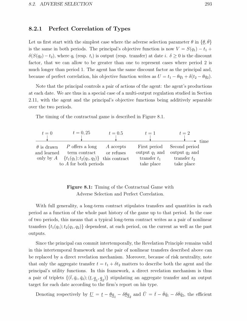
8.2. ADVERSE SELECTION 293
8.2.1 Perfect Correlation of Types
Let us first start with the simplest case where the adverse selection parameter θ in {θ, θ}is the same in both periods. The principal’s objective function is now V = S(q1) − t1 +
δ(S(q2)− t2), where qi (resp. ti) is output (resp. transfer) at date i. δ ≥ 0 is the discount
factor, that we can allow to be greater than one to represent cases where period 2 is
much longer than period 1. The agent has the same discount factor as the principal and,
because of perfect correlation, his objective function writes as U = t1 − θq1 + δ(t2 − θq2).
Note that the principal controls a pair of actions of the agent: the agent’s productions
at each date. We are thus in a special case of a multi-output regulation studied in Section
2.11, with the agent and the principal’s objective functions being additively separable
over the two periods.
The timing of the contractual game is described in Figure 8.1.
- time??? ? ?
t = 0 t = 0, 25 t = 0.5 t = 1 t = 2
θ is drawnand learnedonly by A
P offers a longterm contract
{t1(q1); t2(q1, q2)}to A for both periods
A accepts
or refusesthis contract
First periodoutput q1 and
transfer t1take place
Second periodoutput q2 and
transfer t2take place
Figure 8.1: Timing of the Contractual Game with
Adverse Selection and Perfect Correlation.
With full generality, a long-term contract stipulates transfers and quantities in each
period as a function of the whole past history of the game up to that period. In the case
of two periods, this means that a typical long-term contract writes as a pair of nonlinear
transfers {t1(q1); t2(q1, q2)} dependent, at each period, on the current as well as the past
outputs.
Since the principal can commit intertemporally, the Revelation Principle remains valid
in this intertemporal framework and the pair of nonlinear transfers described above can
be replaced by a direct revelation mechanism. Moreover, because of risk neutrality, note
that only the aggregate transfer t = t1 + δt2 matters to describe both the agent and the
principal’s utility functions. In this framework, a direct revelation mechanism is thus
a pair of triplets {(t, q1, q2); (t, q1, q
2)} stipulating an aggregate transfer and an output
target for each date according to the firm’s report on his type.
Denoting respectively by U = t − θq1− δθq
2and U = t − θq1 − δθq2, the efficient

294 CHAPTER 8. DYNAMICS UNDER FULL COMMITMENT
and the inefficient agents’ information rents over both periods, the following incentive
constraints must thus be satisfied:
U ≥ U + ∆θ(q1 + δq2), (8.1)
U ≥ U −∆θ(q1+ δq
2). (8.2)
The intertemporal participation constraints of both types are respectively:
U ≥ 0, (8.3)
U ≥ 0. (8.4)
Remark: Note that those participation constraints stipulate that only the agent’s in-
tertemporal rent must be positive. So, we assume momentarily that agent commits to
stay in the relationship once he has accepted the contract at date 0. In period 1, the
agent can make a loss if it is covered by a gain in period 2 and vice versa.
The principal’s problem becomes:
(P ) : max{(U,q
1,q
2),(U ,q1,q2)}
ν(S(q
1)− θq
1+ δ(S(q
2)− θq
2)− U
)
+(1− ν)(S(q1)− θq1 + δ(S(q2)− θq2)− U
),
subject to (8.1) to (8.4).
Of course, the relevant constraints are, again, the efficient type’s incentive constraint
(8.1) and the inefficient type’s participation constraint (8.4). For the optimal dynamic
contract only the efficient type gets a positive intertemporal rent which is worth U =
∆θ(q1 + δq2) and the inefficient type’s participation constraint is binding so that U = 0.
Inserting these expressions of the intertemporal rents into the principal’s objective func-
tion and optimizing with respect to outputs, we get immediately the following proposition
where we index this solution with a superscript “D” meaning “dynamics”.
Proposition 8.1 : With perfectly correlated types, the optimal dynamic contract over
two periods is twice the repetition of the optimal static contract.
• The efficient agent produces efficiently in both periods, qD1
= qD2
= qD = q∗ such
that S ′(q∗) = θ.

8.2. ADVERSE SELECTION 295
• The inefficient agent produces less than the first-best output in both periods, qD1 =
qD2 = qD ≤ q∗ such that:
S ′(qD) = θ +ν
1− ν∆θ. (8.5)
It is the same output as in the optimal static contract qD = qSB.
• Only the efficient agent gets a positive intertemporal rent UD = ∆θ(1 + δ)qD.
Remark 1: Note that, even if the optimal long term contract implements the same
output levels and the same intertemporal rents as the optimal static contract of Chapter
1 repeated twice, some indeterminacy remains concerning the intertemporal distribution
of these rents.
Remark 2: Let us instead assume that the principal offers to the agent a contract covering
both periods at the ex ante stage, i.e., before the agent learns his private information.
Moreover, let us consider the case where the agent has an infinite degree of risk aversion
below zero wealth. In that case, the agent’s intertemporal participation constraints (8.3)
and (8.4) would have been replaced respectively by a pair of participation constraints for
each period, namely, U1 = t1 − θq1≥ 0, U2 = t2 − θq
2≥ 0 and U1 = t1 − θq1 ≥ 0,
U2 = t2 − θq2 ≥ 0. Under those assumptions, the same result as in Proposition 8.1 still
holds. Moreover, because the agent would have a positive rent in any given period, there
would be no need for him to commit to stay in the relationship. The agent would never
have the incentive to renege on the long-term contract offered by the principal.
We let the reader check that the outputs implemented in the optimal intertemporal
contract are again given by Proposition 8.1. The main difference with the case of risk
neutrality is that the intertemporal distribution of rents is now completely defined. The
efficient type gets a positive rent in both periods UDi = ∆θqD, for i = 1, 2. The
inefficient type gets instead zero in both periods.
Importantly, Proposition 8.1 shows the importance of the principal’s ability to commit.
If the firm is inefficient, this fact is now common knowledge at the beginning of period 2.
Still, the principal implements an inefficient contract with under-production. We come
back to this commitment issue in Section 8.4 below.
The dynamics of the optimal contract with full commitment was first established
in different settings by Roberts (1983) and Baron and Besanko (1984b). At a more
abstract level, the applicability of the Revelation Principle to a dynamic context (with
possibly more complex information structures than those with perfect correlation) was
demonstrated by Myerson (1986) and Forges (1986) (see also Myerson (1991) for a review
of the argument).
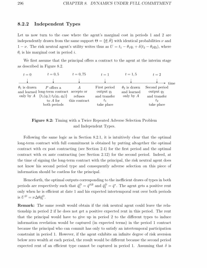
296 CHAPTER 8. DYNAMICS UNDER FULL COMMITMENT
8.2.2 Independent Types
Let us now turn to the case where the agent’s marginal cost in periods 1 and 2 are
independently drawn from the same support Θ = {θ, θ} with identical probabilities ν and
1− ν. The risk neutral agent’s utility writes thus as U = t1 − θ1q1 + δ(t2 − θ2q2), where
θi is his marginal cost in period i.
We first assume that the principal offers a contract to the agent at the interim stage
as described in Figure 8.2.
- time??????
t = 0 t = 0, 5 t = 0, 75 t = 1 t = 1, 5 t = 2
P offers along-term contract{t1(q1); t2(q1, q2)}
to A forboth periods
Aaccepts or
refusesthis contract
θ1 is drawnand learnedonly by A
First periodoutput q1
and transfert1
take place
θ2 is drawnand learnedonly by A
Second periodoutput q2
and transfert2
take place
Figure 8.2: Timing with a Twice Repeated Adverse Selection Problem
and Independent Types.
Following the same logic as in Section 8.2.1, it is intuitively clear that the optimal
long-term contract with full commitment is obtained by putting altogether the optimal
contract with ex post contracting (see Section 2.4) for the first period and the optimal
contract with ex ante contracting (see Section 2.12) for the second period. Indeed, at
the time of signing the long-term contract with the principal, the risk neutral agent does
not know his second period type and consequently adverse selection on this piece of
information should be costless for the principal.
Henceforth, the optimal outputs corresponding to the inefficient draws of types in both
periods are respectively such that qD1 = qSB and qD
2 = q∗. The agent gets a positive rent
only when he is efficient at date 1 and his expected intertemporal rent over both periods
is UD = ν∆θqD1 .
Remark: The same result would obtain if the risk neutral agent could leave the rela-
tionship in period 2 if he does not get a positive expected rent in this period. The rent
that the principal would have to give up in period 2 to the different types to induce
information revelation would be captured (in expected terms) in the period 1 contract
because the principal who can commit has only to satisfy an intertemporal participation
constraint in period 1. However, if the agent exhibits an infinite degree of risk aversion
below zero wealth at each period, the result would be different because the second period
expected rent of an efficient type cannot be captured in period 1. Assuming that δ is

8.2. ADVERSE SELECTION 297
small enough and that this rent can be captured in period 1 from an efficient type, we
obtain the solution characterized in Proposition 8.2 below for the case ν2(θ) = ν2(θ) = ν1.
8.2.3 Correlated Types
Let us generalize the previous information structure and turn now to the more general
case where the agent’s types are imperfectly correlated over time. In this framework, a
direct mechanism requires that the agent reports at each date the new information he has
learned on his current type. Typically, a direct revelation mechanism is thus a four-uple{t1(θ1), t2(θ1, θ2), q1(θ1), q2(θ1, θ2)
}for all pairs (θ1, θ2) belonging to Θ2, where θ1 (resp.
θ2) is date 1 (resp. date 2) announcement on his first period (resp. second period) type.
The important point to note here is that the first period report can now be used by
the principal to update his beliefs on the agent’s second period type. This report can be
viewed as a soft information signal to improve second period contracting. This idea is
quite similar to that seen in Section 2.15.1. The difference is that, now, the signal used
by the principal to improve second period contracting is not exogenously given by nature
but comes from the first period report of the agent on his type in this latter period.
Let us assume that the contract is offered ex ante and that the agent is infinitely risk
averse below zero wealth in both periods, i.e., has a utility function:
u(x) =
{x if x ≥ 0,
−∞ if x < 0.(8.6)
This definition of the utility function imposes that the agent’s payoff in any period
must remain positive whatever his type.5
We denote by ν1 (resp. 1 − ν1) the probability that the first period cost is θ (resp.
θ). Similarly, we denote by ν2(θ1) (resp. 1− ν2(θ1)) the second period probabilities that
the agent is efficient (resp. negative) following a cost realization θ1 in the first period. A
positive correlation between costs in both periods is thus obtained when ν2(θ) > ν2(θ).
In period 2, following a first period report θ1 made by the agent, the principal will
choose outputs q2(θ1) for the efficient type and q2(θ1) for the inefficient type and propose
second period rents U2(θ1) and U2(θ1). Of course, we have U2(θ1) = t2(θ1)− θq2(θ1) and
U2(θ1) = t2(θ1)− θq2(θ).
The agent being infinitely risk averse below zero wealth, the ex post participation
5The same constraints would obtain if the contract was offered after the agent discovers θ1 and if thereis no commitment for the agent to stay in the relationship.

298 CHAPTER 8. DYNAMICS UNDER FULL COMMITMENT
constraint in period 2
U2(θ1) ≥ 0 (8.7)
is binding for any first period announcement θ1 belonging to Θ.
Moreover, inducing information revelation by the agent when he is efficient in period
2 requires to have:
U2(θ1) ≥ U2(θ1) + ∆θq2(θ1), (8.8)
for any first period announcement θ1. As usual this incentive constraint for date 2 is
binding at the optimum.
In period 2, the second period optimal contract following any announcement θ1 must
thus solve the problem below:
(P (θ1)) : max{(q
2(θ1),U2(θ1));(q2(θ1),U2(θ1))}
ν2(θ1)(S(q
2(θ1))− θq
2(θ1)− U2(θ1)
)
+(1− ν2(θ1))(S(q2(θ1))− θq2(θ1)− U2(θ1)
)subject to (8.7) and (8.8).
(8.7) and (8.8) being both binding, the principal’s second period profit, that we denote
thereafter by V2
(θ1, q2
(θ1), q2(θ1)), writes as a function of second period outputs as:
V2
(θ1, q2
(θ1), q2(θ1))
= ν2(θ1)(S(q
2(θ))− θq
2(θ1)
)+(1− ν2(θ1))
(S(q2(θ1))− θq2(θ1)
)− ν2(θ1)∆θq2(θ1). (8.9)
Let us now move backwards to period 1. Knowing what will be the consequences of
his first period report θ1 on the principal’s updated beliefs, the agent with a low first
period cost will truthfully reveal his type whenever the following intertemporal incentive
constraint is satisfied:
U1 + δν2(θ)∆θq2(θ) ≥ U1 + ∆θq1 + δν2(θ)∆θq2(θ). (8.10)
where U1 = t1 − θq1
and U1 = t1 − θq1 are the first period rents.
The terms δν2(θ)q2(θ) and δν2(θ)q2(θ) represent the expected information rents that
the agent can get in the second period continuation of the contract if he reports respec-
tively θ1 = θ or θ1 = θ to the principal, knowing that the probability of his second period
type is θ is ν2(θ).

8.2. ADVERSE SELECTION 299
Similarly, the agent with a high first period cost truthfully reveals when:
U1 + δν2(θ)∆θq2(θ) ≥ U1 −∆θq1+ δν2(θ)∆θq2(θ). (8.11)
Again, infinite risk aversion below zero wealth requires that the ex post participation
constraints
U1 ≥ 0, (8.12)
U1 ≥ 0, (8.13)
be both satisfied.
The principal’s problem writes thus as:
(P ) : max{(q
1,q
2(θ),q2(θ),U1);(q1,q
2(θ),q2(θ),U1)}
ν1
(S(q
1)− θq
1− U1
)+ (1− ν1)
(S(q1)− θq1 − U1
)+δ
(ν1V2(θ, q2
(θ), q2(θ)) + (1− ν1)V2(θ, q2(θ), q2(θ))
)subject to (8.10) to (8.13).
We let the reader check that the two relevant constraints are again the incentive con-
straint (8.10) and the participation constraint (8.13). The next proposition summarizes
the dynamics of the optimal long-term contract.
Proposition 8.2 : The optimal long-term contract with full commitment entails:
• Constraints (8.10) and (8.13) are both binding.
• The agent always produces the first-best output qD1
= qD2(θ) = qD
2(θ) = q∗ when he
is efficient.
• The agent produces generally below the first-best output when he is inefficient.
In period 1, the inefficient agent produces:
S ′(qD1 ) = θ +
ν1
1− ν1
∆θ. (8.14)
In period 2, following θ1 = θ, the inefficient agent produces:
S ′(qD2 (θ)) = θ +
(ν2(θ)
1− ν2(θ)+
ν1ν2(θ)
(1− ν1)(1− ν2(θ))
)∆θ, (8.15)
In period 2, following θ1 = θ, the inefficient agent produces the first-best output
qD2 (θ) = q∗.

300 CHAPTER 8. DYNAMICS UNDER FULL COMMITMENT
• The agent’s expected information rent over both periods is:
UD = ∆θ(ν1q
D1 + δ(ν1ν2(θ)q
D2 (θ) + (1− ν1)ν2(θ)q
D2 (θ))
). (8.16)
In this proposition we have assumed that the first period participation constraint of
the efficient type was never binding. Indeed, when (8.10) and (8.13) are both binding, we
have UD1 = ∆θqD
1 + δ∆θ(qD2 (θ)− qD
2 (θ)) and UD1 is positive as long as the first period rent
∆θqD1 is larger than the second period expected rent differential δν2(θ)∆θ(qD
2 (θ)− qD2 (θ)).6
Then, for an agent who is efficient in the first period, the second period expected rent
can be recaptured in period 1 and the principal can afford an efficient production level
qD2 (θ) = q∗ for the inefficient type in period 2 following an announcement of θ in period 1.
However, for an inefficient agent who has no rent in period 1, this is not possible. Hence,
the principal requires some output distortion for an inefficient type in period 2 following
the announcement of θ in period 1.
Note that those results encompass both the case of independent draws and the case
of perfectly correlated draws when the agent is infinitely risk averse below zero wealth in
both periods. For independent draws, we have ν2(θ) = ν2(θ) = ν1 and we find that the
second period average marginal surplus is Eθ1
(S ′(qD2 (θ1))) = θ+ ν1
1−ν1∆θ where E
θ1
(·) denotes
the expectation operator with respect to θ1. In the case of perfectly correlated types, we
have instead ν2(θ) = 0 and ν2(θ) = 1. Hence, we obtain immediately (as in Section
8.2.1) that the only second period inefficient output given with a positive probability is:
S ′(qD2 (θ)) = θ + ν1
1−ν1∆θ and thus qD
2 (θ) = qD1 .
More generally, decreasing (resp. increasing) qD2 (θ) (resp. qD
2 (θ)) below (resp. above)
qD1 helps the principal to reduce the intertemporal incentive constraint of an agent who
has a low cost in the first period as it can be easily seen on (8.10).
Baron and Besanko (1984b) derived optimal contracts with types correlated
over time and full commitment of the principal. Laffont and Tirole (1996) provided an
application of dynamic contracting models with adverse selection to explain the regulation
of pollution rights as well as an interpretation of the optimal mechanisms in terms of
markets with options. The case of types independently distributed has also been used in
models of infinitely repeated relationships starting with Townsend (1982), Green (1987),
Phelan and Townsend (1990), Green and Oh (1991), Atkeson and Lucas (1992), Thomas
and Worall (1990) and Wang (1995). Those papers are interested in deriving the properties
of the long run distribution of the agent’s utility and consumption and draw sometimes
some macroeconomic implications of the analysis of these distributions. Generally, they
6Note that this condition always holds for δ small enough.

8.3. A DIGRESSION ON NON-COMMITMENT 301
also assume that screening in a one-shot relationship is not feasible since the principal has
only one instrument to control the agent. In a long-term relationship the specification
of the continuation payoffs of the contracts is then the second crucial instrument needed
to screen the agent. In Section 8.3.4 below, we will analyze for the case of moral hazard
some of the recursive techniques used in this latter literature to characterize the optimal
long-term contract.
8.3 A Digression on Non-Commitment
From the analysis above, it appears that the generalization of incentive theory to a dy-
namic context is straightforward provided that the principal has the ability to commit.
However, in the case where there is some correlation of types between both periods,
the principal could use the information learned over time to propose a renegotiation of
the initial long-term contract he has initially offered to improve the terms of the rent
extraction-efficiency trade-off over the course of the contract. In other words, this op-
timal long-term contract may fail to be renegotiation-proof. In Section 2.11, we have
already touched on this commitment issue in one-shot relationships, arguing that simple
indirect mechanism can be a way around this commitment problem and that the possibil-
ity for renegotiating the contract comes only as an artefact of the use of a direct revelation
mechanism between the principal and the agent. In an intertemporal context, the com-
mitment problem is much more a concern because the course of actions leaves open dates
for recontracting. It is out of the purpose of this volume to solve for the optimal dynamic
renegotiation-proof long-term contract. However, we provide in Section 9.3 a few remarks
and some preliminary formal analysis for this case.
8.4 Moral Hazard
8.4.1 The Model
We come back to the framework of Chapter 4, but now, we assume that the relationship
between the principal and the agent is repeated for two periods. The risk averse agent
has thus an intertemporal utility given by U = u(t1) − ψ(e1) + δ(u(t2) − ψ(e2)), where
ti (resp. ei) is the agent’s transfer (resp. effort) at date i. Again, we assume that ei
belongs to {0, 1} with disutilities normalized as usual as ψ(1) = ψ and ψ(0) = 0. In
each period, the agent’s effort yields a stochastic return qi = q (resp. q) with probability
π(ei) (resp. 1 − π(ei)). We denote π0 = π(0), π1 = π(1) and ∆π = π1 − π0. Stochastic
returns are independently distributed over time so that the past history of realizations

302 CHAPTER 8. DYNAMICS UNDER FULL COMMITMENT
does not yield any information on the current likelihood of a success or a failure of the
production process. As usual, the principal is risk neutral and has a separable utility
function V = S(q1)− t1 + δ(S(q2)− t2).
In this two period environment, the principal offers a long-term contract to the agent.
In full generality, this contract involves transfers at each date which are contingent
on the whole past history of outcomes. Typically a long-term contract writes thus as
{t1(q1), t2(q1, q2)} where q1 and q2 are output realizations in periods 1 and 2 respectively.
Such a contract stipulates thus 2 + 2 × 2 = 6 possible transfers depending on the real-
izations of outcomes. For simplicity of notation, we will use t1(q) = t1 and t1(q) = t1 to
denote first period first period transfers. Similarly, t2(q1) and t2(q1) denote transfers in
the second period. As usual, the description of participation and incentive constraints is
easier when one introduces the new variables u1 = u(t1), u1 = u(t1), u2(q1) = u(t2(q1))
and u2(q1) = u(t2(q1)).
For further references, the timing of the game is shown in Figure 8.3 below:
- time??????
t = 0 t = 0, 5 t = 0, 75 t = 1 t = 1, 5 t = 2
P offers along-term contract{t1(q1); t2(q1, q2)}
to A
Aaccepts or
refusesthis contract
A exertseffort e1
First periodoutput q1 isrealized and
transfert1(q1) is paid
A exertseffort e2
Second periodoutput q2 isrealized and
transfert2(q1, q2) is paid
Figure 8.3: Timing with a Twice Repeated Moral Hazard Problem.
Remark: The reader will have recognized the framework of a multi-task moral hazard
problem along the lines of that presented in Chapter 5. There are two main differences.
First, the sequentiality of actions which are now taken at different dates implies that
payments take place also at two different dates. Second, the separability of the agent’s
disutility of efforts over time will allow a somewhat simpler characterization of the optimal
contract as we will see below.
8.4.2 The Optimal Long-Term Contract
We focus on the case where effort is extremely valuable for the principal who always wants
to implement a high level of effort in both periods. We can thus describe the second period
incentive constraints as:
u2(q1)− u2(q1) ≥ ψ
∆πfor all q1 in {q, q}. (8.17)

8.4. MORAL HAZARD 303
In full generality, these constraints obviously depend on the first period level of output
q1, i.e., on the history of past performances.
Let us move backwards. In period 1, the agent anticipates his future stream of random
payoffs to evaluate the current benefit of exerting a first period effort or not. The first
period incentive constraint writes thus as:
u1 + δ(π1u2(q) + (1− π1)u2(q))−(u1 + δ(π1u2(q) + (1− π1)u2(q))
) ≥ ψ
∆π. (8.18)
The terms u1 and u1 represent the current utilities associated with the transfers received
by the agent in period 1 depending on the realized production. The terms δ(π1u2(q) +
(1− π1)u2(q)) and δ(π1u2(q) + (1− π1)u2(q)) represent the discounted expected utilities
associated with the transfers received by the agent in period 2 following each possible
first period output. Clearly, these continuations affect the first period incentives to exert
effort.
Finally, the agent accepts the long-term contract before q1 and q2 realize. His in-
tertemporal participation constraint writes as:
π1 (u1 + δ(π1u2(q) + (1− π1)u2(q)))
+(1− π1)(u1 + δ(π1u2(q) + (1− π1)u2(q))
)− (1 + δ)ψ ≥ 0. (8.19)
Denoting again by h = u−1 the inverse function of the agent’s utility function, the
principal’s problem is to solve:
(P ) : max{(u1;u1);(u2(q),u2(q),u2(q),u2(q))}
π1
(S − h(u1) + δ(π1(S − h(u2(q)) + (1− π1)(S − h(u2(q))))
)+(1− π1)
(S − h(u1) + δ(π1(S − h(u2(q)) + (1− π1)(S − h(u2(q))))
)subject to (8.17) to (8.19).
Solving this problem highlights the particular role played by the agent’s average levels
of utility for the second period following the first period realization q1, namely π1u2(q1)+
(1−π1)u2(q1)−ψ. Indeed, if the agent has been promised an expected second period utility
u2(q1), the levels of utility u2(q1) and u2(q1) must satisfy the second period participation
constraints
π1u2(q1) + (1− π1)u2(q1)− ψ ≥ u2(q1), for any q1. (8.20)
Only these second period continuation payoffs u2(q1) matter from the agent’s point
of view when he has to decide his effort in period 1 and to accept the contract that the
principal has offered.

304 CHAPTER 8. DYNAMICS UNDER FULL COMMITMENT
Given the promise made by the principal (which is credible because of our implicit
assumption of full commitment) of a future utility u2(q1) for the agent following a first
period output q1, the continuation contract for the second period solves the problem
below:
(P2(q1)) : max{u2(q1),u2(q1)}
π1
(S − h(u2(q1))
)+ (1− π1) (S − h(u2(q1)))
subject to (8.17) and (8.20).
We denote by V2(u2(q1)) the value of problem (P2(q1)). This is the principal’s second
period payoff when he has promised a level of utility u2(q1) to the agent.
This problem is almost the same as the static problem of Chapter 4 and its solution
can be derived similarly. The only difference is that the agent receives the promise of
a second period utility u2(q1) when the first period output which has already realized is
q1 instead of zero as in the static model of Chapter 4. Applying the same techniques as
in Chapter 4, it is straightforward to show that both constraints (8.17) and (8.20) are
binding at the optimum. Hence, we can compute the second period agent’s payoffs in
both states of nature as:
uSB2 (q1) = ψ + u2(q1) + (1− π1)
ψ
∆π, (8.21)
and
uSB2 (q1) = ψ + u2(q1)− π1
ψ
∆πfor all q1 in {q, q}. (8.22)
This yields the following expression of the second-best cost CSB2 (u2(q1)) of implement-
ing a high effort in period 2 following the promise of a second period utility u2(q1):
CSB2 (u2(q1)) = π1h
(ψ + u2(q1) + (1− π1)
ψ
∆π
)+ (1− π1)h
(ψ + u2(q1)− π1ψ
∆π
).
(8.23)
Finally, we find the continuation value of the contract for the principal:
V2(u2(q1)) = π1S + (1− π1)S − CSB2 (u2(q1)). (8.24)
For further references, note also that V ′2(u2(q1)) = −CSB′
2 (u2(q1)).
These optimal continuations of the contract being defined, we can now move backwards
to solve for the optimal long-term contract. Taking into account the expressions above,
the principal’s problem (P ) can thus be rewritten as:
(P ′) : max{(u1,u1);(u2(q),u2(q))}
π1(S−h(u1))+(1−π1)(S−h(u1))+δ(π1V2(u2(q)) + (1− π1)V2(u2(q))
)

8.4. MORAL HAZARD 305
subject to
u1 + δu2(q)− (u1 + δu2(q)) ≥ ψ
∆π, (8.25)
π1(u1 + δu2(q)) + (1− π1)(u1 + δu2(q)) ≥ ψ, (8.26)
where (8.25) is the first period incentive constraint and (8.26) the intertemporal participa-
tion constraint. Both constraints are rewritten as functions of the expected continuation
payoffs u2(q) and u2(q). As in Section 8.2 we index the solution to this problem with a
superscript “D” meaning “dynamics.”
Let us introduce the respective multipliers λ and µ of these constraints. (P ′) is a con-
cave problem with linear constraints for which the Kuhn and Tucker first-order conditions
are necessary and sufficient to characterize optimality. Optimizing with respect to u1 and
u1 yields respectively:
π1h′(uD
1 ) = λ + µπ1, (8.27)
(1− π1)h′(uD
1 ) = −λ + µ(1− π1). (8.28)
Summing those two equations, we obtain:
µ = π1h′(uD
1 ) + (1− π1)h′(uD
1 ) > 0, (8.29)
and thus the agent’s intertemporal participation constraint (8.26) is necessarily binding.
Also, from (8.27) and (8.28) we get immediately:
λ = π1(1− π1)(h′(uD
1 )− h′(uD1 )
). (8.30)
Optimizing with respect to u2(q) and u2(q) yields also:
π1CSB′2 (uD
2 (q)) = λ + µπ1, (8.31)
(1− π1)CSB′2 (uD
2 (q)) = −λ + µ(1− π1). (8.32)
Hence, we have another way of writing the multiplier λ as:
λ = π1(1− π1)(CSB′
2 (uD2 (q))− CSB′
2 (uD2 (q))
). (8.33)
Direct identifications of (8.27) with (8.31) and of (8.28) with (8.32) yield respectively:
h′(uD1 ) = CSB′
2 (uD2 (q)) = π1h
′(uD2 (q)) + (1− π1)h
′(uD2 (q)), (8.34)
and
h′(uD1 ) = CSB′
2 (uD2 (q)) = π1h
′(uD2 (q)) + (1− π1)h
′(uD2 (q)). (8.35)

306 CHAPTER 8. DYNAMICS UNDER FULL COMMITMENT
Those two equations show that the following martingale property must be satisfied at
the optimum:
h′(uD1 (q1)) = E
q2
(h′(uD2 (q1)), for all q1 in {q, q}, (8.36)
where Eq2
(·) denotes the expectation operator with respect to the distribution of second
period output q2 induced by a high effort at this date and uD2 is the random value of
second period utilities.
This martingale property shows that the marginal cost of giving up some rent to the
agent in period 1 following any output q1 must be equal to the marginal cost of giving up
rent in the corresponding continuation of the contract.
This property is rather important. It says that, because of the agent’s risk aversion,
the principal spreads intertemporally the agent’s rewards and punishments to minimize
the cost of implementing a high effort in period 1. To give all rewards and punishments
necessary to induce effort in period 1 in this period only is clearly suboptimal. The
principal prefers to smooth the burden of the cost of the incentive constraint between
today and tomorrow.
Moreover, since λ ≥ 0 and CSB′2 (·) is increasing,7 (8.33) implies that uD
2 (q) ≤ uD2 (q).
But the equality is impossible, since, from (8.34) and (8.35), it would imply that uD1 ≤ uD
1
and (8.25) would be violated. Henceforth, the high first period output is not only rewarded
in period 1 but also in period 2. The optimal long-term contract with full commitment
exhibits memory. Note that this memory property implies more generally that the first
period payments and their expected continuations covary positively.
The main features of the optimal contract are summarized in the next proposition.
Proposition 8.3 : With a twice repeated moral hazard problem, the optimal long term
contract with full commitment exhibits memory and the martingale property h′(uD1 (q1)) =
Eq2
(h′(uD2 (q1)) is satisfied.
To get further insights on the structure of the agent’s payments in a long-term rela-
tionship, let us come back to our usual quadratic example and assume that h(u) = u+ ru2
2
for some r > 0. The martingale property (8.36) yields immediately that uD1 (q1) =
π1uD2 (q1) + (1 − π1)u
D2 (q1), for all q1 in {q, q}. Inserting those equalities into (8.25) and
(8.26) yields respectively uD1 − uD
1 = ψ∆π(1+δ)
and π1uD1 + (1− π1)u
D1 = ψ.
7This monotonicity is obtained because h(·) is convex.

8.4. MORAL HAZARD 307
Finally, the structure of the payments at each date can be fully derived as:
uD1 = ψ +
(1− π1)ψ
∆π(1 + δ), (8.37)
uD1 = ψ − π1ψ
∆π(1 + δ), (8.38)
uD2 (q) = ψ +
(1− π1)ψ
∆π(1 + δ)+
(1− π1)ψ
∆π, (8.39)
uD2 (q) = ψ +
(1− π1)ψ
∆π(1 + δ)− π1ψ
∆π, (8.40)
uD2 (q) = ψ − π1ψ
∆π(1 + δ)+
(1− π1)ψ
∆π, (8.41)
uD2 (q) = ψ − π1ψ
∆π(1 + δ)− π1ψ
∆π. (8.42)
The values of these transfers immediately highlight two phenomena. First, compared
with a static one-shot relationship, the first period power of incentives needed to induce a
first period effort is lower. A factor 11+δ
< 1 reduces the risk borne by the agent during this
first period in order to induce effort at this date. Second, an early success (resp. failure)
is translated into future compensations which are shifted upwards (resp. downwards).
This captures the effect of the past history of performances on future compensations.
Malcomson and Spinnewin (1988), Rogerson (1985b) and Lambert (1983) have
all shown that the optimal long-term contract exhibits memory. Rey and Salanie (1990)
have shown how long-term contracts can be generally replaced by two period short-term
contracts in a framework with T periods. Chiappori, Macho, Rey and Salanie (1994)
offers an interesting survey of the literature.
Proposition 8.3 provides a useful benchmark with respect to which we can assess the
impact of various limitations that the principal may face in contracting with the agent in
a long-term relationship.
8.4.3 Renegotiation-Proofness
Importantly, the recursive procedure that we have used in Section 8.4.2 to compute the
optimal long-term contract shows that it is in fact sequentially optimal. Given the promise
u2(q1) made by the principal following a first period outcome q1, there is no point for the
principal in offering another contract than the continuation for the second period of the
optimal long-term contract above. By definition, the optimal long-term contract is thus
renegotiation-proof.

308 CHAPTER 8. DYNAMICS UNDER FULL COMMITMENT
8.4.4 Reneging on the Contract
In the previous analysis, once accepted, the optimal contract with full commitment has
only a single participation constraint. This contract forces the agent to stay in the re-
lationship in period 2 even if his expected payoff is then negative. This a rather strong
assumption on the enforcement of a contract. Suppose now that the agent cannot commit
himself to stay in a relationship if he gets less than his reservation value normalized at
zero. To avoid any breach of contract, the average promised payoffs u2(q1) following a
first period output q1 must now satisfy the second period participation, or renegation-
proofness, constraints:
u2(q1) ≥ 0, for all q1 in {q, q}. (8.43)
Considering the possibility of a breach of contract puts therefore further constraints
on the principal’s problem (P ′). If he were unconstrained, the principal would like to
decrease u2(q) and increase u2(q) because playing on future promises helps to provide
also first period incentives as equation (8.26) has already shown us. However, diminishing
u2(q) until its optimal value with no renegation of contract conflicts now with the second
period participation constraints (8.43). Indeed, using (8.41) and (8.42), we observe that
the optimal long-term contract always violates constraint (8.43) since uD2 (q) = π1u
D2 (q) +
(1 − π1)uD2 (q) − ψ = − π1ψ
∆π(1+δ)< 0. Hence, when the agent can walk away from the
relationship in the second period, the constraint (8.43) must be binding following a low
first period output. The principal is then strongly limited in the second period punishment
he can inflict to the agent following such a history of the game.
The optimal renegation-proof contract entails thus (8.43) being binding for q1 = q.
Following such a low first period output, it should be clear that the continuation contract
is the replica of the static contract of Chapter 4. Let us now derive the other components
of the long-term contract, i.e., the levels of utilities in the first period contract and in the
second period following a high first period continuation output q1 = q. The intertemporal
incentive constraint writes now as:
u1 + δu2(q)− u1 ≥ψ
∆π. (8.44)
Similarly, the intertemporal participation constraint is obtained as:
π1(u1 + δu2(q)) + (1− π1)u1 ≥ ψ. (8.45)
Taking into account the binding renegation-proofness constraint u2(q) = 0, the prin-
cipal’s problem can be rewritten as:

8.4. MORAL HAZARD 309
(P ) : max{(u1,u1);u2(q)}
π1
(S − h(u1) + δV2(u2(q)
)+ (1− π1) (S − h(u1) + δV2(0))
subject to (8.44) and (8.45).
We index with a superscript “R” meaning “renegation-proof” the solution to this
problem. We denote now by λ and µ the respective multipliers of the two constraints of
(P ). The corresponding first-order conditions obtained by optimizing with respect to u1,
u1 and u2(q) write as:
−π1h′(uR
1 ) + λ + µπ1 = 0, (8.46)
−(1− π1)h′(uR
1 )− λ + µ(1− π1) = 0, (8.47)
−π1CR′2 (uR
2 (q)) + λ + µπ1 = 0, (8.48)
where uR1 and uR
2 are the optimal payoffs in the first period and uR2 (q) is the optimal
continuation payoffs following a high output in the first period.
Summing (8.46) to (8.47), we obtain µ = π1h′(uR
1 ) + (1 − π1)h′(uR
1 ) > 0, and the
participation constraint (8.45) is binding. Inserting this value of µ into (8.46), we finally
get λ = π1(1− π1)(h′(uR
1 )− h′(uR1 )). Using (8.46) and (8.48) we also obtain that:
h′(uR1 ) = CSB′
2 (uR2 (q))
= π1h′(
ψ + uR2 (q) +
(1− π1)ψ
∆π
)+ (1− π1)h
′(
ψ + uR2 (q)− π1ψ
∆π
).(8.49)
This equation is again a martingale property which now applies only following a first
period success. Smoothing the rewards for a first period success between the two periods
calls for equalizing the agent’s utility in period 1 with its future expected value in period
2.
Using the quadratic specification of h(·), we find that
uR1 = uR
2 (q) + ψ = π1uR2 (q) + (1− π1)u
R2 (q). (8.50)
We let as an exercice to the reader to check that necessarily λ > 0.
Using (8.50) with the binding constraints (8.44) and (8.45) yields a linear system with
three unknowns and three equations. Solving this system, we first obtain the following
expressions of ex post utilities in each state of nature: uR1 = ψ + (1−π1)ψ
∆π(1+δ), uR
1 = ψ − π1ψ∆π
,
uR2 (q) = ψ + (1−π1)ψ
∆π(1+δ)+ (1−π1)ψ
∆π, uR
2 (q) = ψ + (1−π1)ψ∆π(1+δ)
− π1ψ∆π
. Taking into account that
uR2 (q) = 0, we have also uR
2 (q) = ψ + (1−π1)ψ∆π
and uR2 (q) = ψ − π1ψ
∆π.
Comparing these expressions of the ex post utilities with those obtained when the
agent cannot leave the relationship in period 2, we get the next proposition.
310 CHAPTER 8. DYNAMICS UNDER FULL COMMITMENT
Proposition 8.4 : Assume that h(·) is quadratic, with a twice repeated moral hazard
problem and a renegation-proofness constraint, the optimal long-term contract is the same
as with full commitment except for the payoffs corresponding to a low first period output:
uR1 < uD
1 , uR2 (q) > uD
2 (q), and uR2 (q) > uD
2 (q).
The renegation-proofness constraint (8.43) affects quite significantly the structure of
the agent’s payoffs following a low first period output. However, the optimal long-term
contract still exhibits memory and tracks the agent’s performances over time as with full
commitment. An early success implies also some greater rewards later on. Because the
principal can no longer spread a punishment following a low first period output q1 = q
between period 1 and period 2, all this punishment must be inflicted to the agent in the
first period.8 Following such a low first period output, the agent receives in period 2 the
optimal static contract corresponding to a zero participation constraint.
8.4.5 Saving
In the framework of Section 8.4.2, we have assumed that the principal has the full abil-
ity to restrict the agent’s access to the capital market. This seems a rather strong
assumption, in particular, given the fact that the agent would like to save a positive
amount in the first period when he receives the second best optimal long-term contract
that we have described in Proposition 8.3. To see this point, consider the impact of
saving an amount s in the first period. The agent’s expected utility writes thus as
u(tD1 (q1) − s) + δEq2
(u
(tD2 (q1, q2) + (1 + R)s
)), where, in a perfect credit market, the
interest rate is 1 + R = 1δ
and where Eq2
denotes the expectation operator with respect
to the second period production induced by a high effort. Marginally increasing s above
zero improves the agent’s intertemporal utility whenever:
−u′(tD1 (q1)) + Eq2
(u′(tD2 (q1, q2))
)> 0. (8.51)
Because the optimal contract satisfies the martingale property (8.36), we have also1
h′(uD1 (q1))
= 1Eq2
(h′(uD2 (q1)))
< Eq2
(1
h′(uD2 (q1))
), where the last inequality is obtained by applying
Jensen’s inequality to the strictly convex function 1x. Finally, using 1
h′(uD1 (q1))
= u′(tD1 (q1))
and 1h′(uD
1 (q1))= u′(tD2 (q1, q2)), we obtain that the strict inequality (8.51) holds and a
positive saving is thus optimal.
8In more general models, the principal may also be willing to increase the rewards offered to the agentin case of a success to restore efficient incentives. The renegation-proofness constraint along a path wherethe agent has performed poorly may also have an impact on a path where the agent has performed better.

8.4. MORAL HAZARD 311
More generally, the amount of money saved by the agent being non observable by the
principal, it plays the role of another moral hazard variable which can only be indirectly
controlled by the principal through the long-term contract he offers.
Let us now characterize some features of the optimal contract with saving. First, note
that, given a first period output q1 and any long-term contract {t1(q1); t2(q1, q2)}, the
agent chooses to save an amount s∗(q1) such that it equalizes his marginal utilities of
income in both periods:
u′(t1(q1)− s∗(q1)) = Eq2
(u′
(t2(q1, q2) +
1
δs∗(q1)
)), for any q1 in {q, q}. (8.52)
When s∗(q1) < 0, the agent is in fact borrowing from the capital market. Note that
the agent’s objective function being strictly concave in s, saving is always deterministic.
In computing the expectation above, we have assumed that the agent anticipates that
he will exert a high effort in period 2 so that the probability that q2 is equal to q is π1.
Of course the choice of effort in the continuation is in fact endogenous and depends on
how much the agent would like to save. We come back to this issue below.
By shifting income from one period to the other, the agent is able to play on the
incentive power of the long-term contract he receives from the principal. Now let us
imagine that the principal replaces this initial contract by a new long-term contract
{t1(q1); t2(q1, q2)} which is designed to replicate the agent’s choice and the final allo-
cation of utilities that the latter gets in each state of nature. This new contract should
thus satisfy t1(q1) = t1(q1)− s∗1(q1), for all q1 in {q, q}, and t2(q1, q2) = t2(q1, q2)+ 1δs∗1(q1),
for all (q1, q2) in {q, q}2. With this new contract, the marginal utilities of income are the
same in both periods since by definition:
u′(t1(q1)) = Eq2
(u′(t2(q1, q2)), for all q1 in {q, q}; (8.53)
and the agent chooses neither to save nor to borrow. Moreover, the intertemporal costs
of both contracts are the same for the principal since:
t1(q1) + δEq2
(t2(q1, q2)) = t1(q1) + s∗1(q1) + δEq2
(t2(q1, q2)− 1
δs∗1(q1))
= t1(q1) + δEq2
(t2(q1, q2)), for all q1 in {q, q}. (8.54)
Hence, there is no loss of generality in restricting the principal to offer saving-proof
long-term contracts.
The saving-proofness constraint, however, imposes that the following martingale prop-
erty, obtained from (8.53), be satisfied:
1
h′(u1(q1))= E
q2
(1
h′(u2(q1, q2))
), for any q1 in {q, q}. (8.55)
312 CHAPTER 8. DYNAMICS UNDER FULL COMMITMENT
(8.55) constrains significantly the set of implementable allocations and raises the
agency cost of implementing a high effort. The principal can no longer spread the future
expected payoffs u2(q) and u2(q) as he would like to facilitate the first period provision of
incentives without inducing saving.
The martingale property (8.55) is not the only constraint on the principal’s problem.
Indeed, it would be the case if the stochastic production process in period 2 were exoge-
nous. However, under moral hazard, the choice of effort in this period is endogenous: it
depends on the past consumption made in the first period and the current contract in a
rather complex way. This means that, if the principal can be restricted to saving-proof
long-term contracts on the equilibrium path, this restriction is no longer valid when the
agent decides to change his first period saving so that he prefers exerting low effort in
the second period continuation. Given a long-term contract {t1(q1), t2(q1, q2)} which is
saving-proof on the equilibrium path, the agent, by saving s0 and exerting no effort in
period 2, gets u(t1(q1)− s0) + δ(π0u
(t2(q1, q) + s0
δ
)+ (1− π0)u
(t2(q1, q) + s0
δ
)).
To induce the agent to exert effort in period 2, the following incentive constraint must
thus be satisfied by a saving-proof long term contract:
u(t1(q1)) + δ(π1u(t2(q1, q)) + (1− π1)u(t2(q1, q)))− δψ
≥ max{s0} u(t1(q1)− s0) + δ(π0u
(t2(q1, q) + s0
δ
)+ (1− π0)u
(t2(q1, q) + s0
δ
)).(8.56)
Let us thus consider a second period contract such that t2(q1, q) > t2(q1, q) for any
q1 in {q, q}. It should be noticed that s∗0 defined as the maximizer of the right-hand-side
above is such that:
u′(t1(q1)− s∗0) = π0u′(
t2(q1, q) +s∗0δ
)+ (1− π0)u
′(
t2(q1, q) +s∗0δ
)
> π1u′(
t2(q1, q) +s∗0δ
)+ (1− π1)u
′(
t2(q1, q) +s∗0δ
),
since u′(·) is decreasing. Using the fact that the agent’s objective function is concave in
s and maximized at zero saving when effort a positive effort is exerted, we can conclude
that s∗0 > 0.
It should be also noticed that this double deviation, both along the saving and the ef-
fort dimension, introduces a positive slackness into the second period incentive constraint.
Indeed, the right-hand side of (8.56) is strictly greater than what the agent can get by not
saving at all and exerting no effort, i.e., u(t1(q1))+δ(π0u(t2(q1, q2)) + (1− π0)u(t2(q1, q2
))).
Simplifying, we get finally: u(t2(q1, q2))− u(t2(q1, q2)) > ψ
δ∆π, for any q1 in {q, q}.
This strict inequality implies that the optimal contract with full commitment and
saving is not sequentially optimal. Indeed, once the first period output has been realized
8.4. MORAL HAZARD 313
and the corresponding zero saving has been made, the principal would like to offer a
renegotiation to the agent in order to have the second period incentive constraint being
instead binding.
The design of the optimal contract with saving and non-commitment is rather
complex. Chiappori et al. (1993) provided some insights on the structure of the solution.
8.4.6 Infinitely Repeated Relationship
The two-period model is a highly stylized view of a long-term principal-agent relationship.
Financial contracts, labor contracts, tenancy contracts are all enduring relationships last-
ing for a long period of time. Let us move now to an infinite horizon model still keeping
the basic framework of Section 8.5.2.9 As we will see below, the design of the optimal
long-term contract still exhibits many of the features of our two period example. The
novelty is that the second period is no longer the end of the relationship. All periods are
alike and the principal faces a similar problem of control in each period. It is rather in-
tuitive to see that the whole structure of the contract is now solved recursively. Given an
initial promise of rent (typically zero) from any period on, the principal computes an op-
timal contract which stipulates not only the agent’s current payments but also determines
what are the utility levels which are promised from that period on following each current
realization of the production process. Then, the continuation of the optimal contract in
any period is similar to the contract itself, with possibly, the principal making different
promises of expected utility to the agent from next period on.
The recursive structure of the optimal contract also implies that the contract at any
given date depends on the whole history of past outcomes only through the utility level
promised following such a history. This utility level can be viewed as a stochastic state
variable which summarizes the past history of the agent’s performances. Therefore, the
optimal contract exhibits the Markov property.10
To better describe the optimal contract, let us denote by V (·) the value function
associated with the following dynamic programming problem:
(P ) : V (U) = max{u,u,U ,U}
π1(S − h(u)) + (1− π1)(S − h(u)) + δ(π1V (U)) + (1− π1)V (U)))
subject to
9Hence, the principal can perfectly control the agent’s access to the capital market.10This feature of the optimal contract could be derived more rigorously; however, for the purpose of
this volume, we contend ourselves with the heuristic argument above.

314 CHAPTER 8. DYNAMICS UNDER FULL COMMITMENT
u + δU − (u + δU) ≥ ψ
∆π, (8.57)
π1(u + δU) + (1− π1)(u + δU)− ψ ≥ U. (8.58)
V (U) is the value of the principal’s problem (P ) in an infinitely repeated relationship
with moral hazard, assuming that the principal wants to induce a high effort in each
period and promise an expected utility level U to the agent over the whole relationship.11
Note that the principal must not only stipulate the current payments of the agents but
also the levels of future utilities U and U which are promised in the continuation of the
contract following the respective realizations of q and q. Constraints (8.57) and (8.58)
are respectively the incentive and participation constraints when an expected amount of
rent U has been promised to the agent. These constraints make explicit the role of these
continuation payoffs. Given that the principal has promised an expected level of utility U
to the agent at a given period, he can get the expected payoff V (U) from that period on.
By offering the continuation payoffs U and U , the principal knows, by the mere definition
of the value function V (·), that he will get himself the continuation payoffs V (U) and
V (U).
Let us denote by λ and µ the respective multipliers of the constraints (8.57) and (8.58).
Assuming the concavity of the value function V (·),12 the optimizations with respect to U
and U yield respectively:
π1V′(U(U)) + λ + π1µ = 0, (8.59)
(1− π1)V′(U(U))− λ + (1− π1)µ = 0, (8.60)
where we make explicit the dependence of the solution on the level of promised utility U .
Summing these two equations, we obtain also:
µ = −E(V ′(U(U))), (8.61)
where E(·) is the expectation operator with respect to the distribution of current output
induced by a high effort.
Optimizing with respect to u and u yields also:
π1h′(u(U)) = λ + π1µ, (8.62)
(1− π1)h′(u(U)) = −λ + (1− π1)µ. (8.63)
Summing these two equations, we finally get
µ = E(h′(u(U))) > 0. (8.64)
11We show in Appendix 8.1 of this chapter that it is optimal to induce a high effort in each period ofthe dynamic problem if it is also optimal to do so in a one-shot relationship similar to that in Chapter 4.
12See Stockey and Lucas (1989, Theorem 4.8, p. 81) who show that such a value function exists and isconcave for a dynamic problem like (P ).

8.4. MORAL HAZARD 315
Hence, the participation constraint (8.58) is necessarily binding.
From equations (8.62) and (8.63), we also derive that
λ = π1(1− π1) (h′(u(U))− h′(u(U)))
= π1(1− π)(V ′(U(U))− V ′(U(U))
). (8.65)
h(·) being convex, (8.65) implies that U(U) ≥ U(U) if and only if u(U) ≥ u(U) when
V (·) is concave. To satisfy (8.57), it cannot be that u(U) ≤ u(U) and U(U) ≤ U(U) hold
simultaneously. Hence, we have necessarily u(U) > u(U) and U(U) < U(U).
The economic interpretation of this condition is clear. In an infinitely repeated re-
lationship, the optimal long-term contract exhibits again the memory property. The
explanation is the same. To smooth the agency costs of the relationship with the agent,
the principal spreads the agent’s rewards and punishments between the current period
and its continuation which now involves the whole future of the relationship.
Moreover, using the Envelope Theorem, we have also V ′(U) = −µ. Hence, the
marginal value function satisfies the martingale property :
V ′(U) = E(V ′(U(U))). (8.66)
This property characterizes how the principal smoothes intertemporally the agent’s
reward over time in such a way that one more unit of utility promised today costs him to-
day exactly what he gains from having less to promise tomorrow following any realization
of output.
In general, it is hard to go any further without computing the value function explicitly.
It is interesting to compute such a value function when h(·) is quadratic, i.e., h(u) = u+ ru2
2
for all u where h(·) is increasing and r > 0. Let us also conjecture a quadratic form for the
value function V (U) = α− βU − γU2
2, for any U in IR, and for some parameters (α, β, γ)
in IR× IR2+ to be defined below.
When the agent exerts a positive effort in each period, the martingale property yields
immediately
U = π1U(U) + (1− π1)U(U). (8.67)
Moreover, using (8.65), we have:
r(u(U)− u(U)) = γ(U(U)− U(U)). (8.68)
Since (8.57) is binding, it yields(
γr
+ δ)(U(U) − U(U)) = ψ
∆π, and using (8.67), we

316 CHAPTER 8. DYNAMICS UNDER FULL COMMITMENT
obtain:
U(U) = U +(1− π1)ψ
(γr
+ δ)∆π, (8.69)
U(U) = U − π1ψ
(γr
+ δ)∆π. (8.70)
Similarly, inserting these values of U(U) and U(U) into the binding participation
constraint (8.58), we get π1u(U) + (1 − π1)u(U) = ψ + U(1 − δ), and, using (8.68), we
obtain (γr
+ δ)(u(U)− u(U)) = ψγ∆πr
.
Solving for U(U) and U(U) and inserting those values into (8.69) and (8.70), we get:
u(U) = ψ + U(1− δ) +(1− π1)ψγ
(γ + rδ)∆π; (8.71)
u(U) = ψ + U(1− δ)− π1ψγ
(γ + rδ)∆π. (8.72)
These latter values of U , U, u and u allow us to compute the value function as:
V (U) = π1S + (1− π1)S − ψ − rψ2
2− π(1−π)ψ2
2∆π2
(r( γ
r)2+γδ
( γr+δ)2
)−1
2(r(1− δ)2 + γδ)U2 − ((1− δ)(1 + r) + δβ)U. (8.73)
Indentifying with the quadratic expression of V (U) yields immediately the following
values of the parameters α, β and γ: α = 11−δ
(π1S + (1− π1)S − ψ − rψ2
2
)− rπ1(1−π1)ψ2
2∆π2 ,
β = 1 + r, and γ = r(1− δ).
Normalizing the length of the period by 1 − δ, it is interesting to note that the per
period value function V (U) writes as:
V (U) = (1− δ)V (U) = W ∗ − (1− δ)rπ1(1− π1)ψ2
2∆π2− (1− δ)(1 + r)U − r(1− δ)2
2U2;
(8.74)
where W ∗ = π1S +(1−π1)S−ψ− rψ2
2is the complete information expected surplus from
inducing a high effort.
From the above expression, it should be clear that, as δ goes to one, the per period
value function converges uniformly towards the first-best expected surplus.
Proposition 8.5 : As δ goes to one, the principal’s per period expected profit in an
infinitely repeated relationship with moral hazard converges towards its first-best value.
The intuition for this result is straightforward. Recall from Chapter 4 that the source
of inefficiency in a static moral hazard problem is the fact that the principal must let the

8.4. MORAL HAZARD 317
risk averse agent bear some risk. The principal benefits from the repetition of the game
since he can thereby spread the agent’s rewards and punishments over time and let the
agent only bear a small fraction of the risk associated with his effort in a given period.
When δ is close to one, the risk borne by the agent in each period is made arbitrarily close
to zero as it can be easily seen by computing the difference u(U) − u(U) = (1 − δ)ψ
∆πwhich converges towards 0 as δ goes to 1. Therefore, the cost of moral hazard in a given
period almost disappears and the first-best level of profit is achieved when δ is close to 1.
Another interpretation of this result should be stressed. As the contractual relationship
is repeated, the risk averse agent is subject to many independent risks which arise at
different points in time. The principal structures the intertemporal contract of the agent
to let him being perfectly diversified. As a result of this complete diversification, the agent
is almost risk neutral and the first-best outcome can be obtained just as in a static model
with risk neutrality.
It is finally interesting to compute the distribution of utilities that the agent gets
after i periods. Given that the martingale property (8.67) holds, the distribution Ui of
utilities which are promised to the agent from any period i on is such that Ui = Eqi+1
(Ui+1)
where Eqi+1
denotes the expectations with respect to the output in period i + 1 when the
agent exerts a positive effort in this period. Using the Law of Iterated Expectations, we
get Eqi
(Ui|qi) = Eqi
(E
qi+1
(Ui+1)
)= E
(qi,qi+1)(Ui+1). Proceeding recursively, we finally obtain
U0 = Eq1
(U1) = Ehi+1
(Ui+1), where U0 = 0 is the agent’s reservation utility at the start of
the relationship and hi+1 = (qi+1, qi, . . . , q1) is the whole history of past outcomes up to
period i + 1. Note that the distribution of output in each period induces a distribution
over all possible histories. The martingale property ensures that the agent’s expected
continuation utility from any date i on taken with respect to the distribution of histories
hi is always zero whatever i.
This property is also useful to compute the whole distribution of expected utilities Ui
from any period i on. The laws of motion are given by (8.69) and (8.70) when γ = r(1−δ).
Figure 8.4 below explains how this distribution evolves over time.

318 CHAPTER 8. DYNAMICS UNDER FULL COMMITMENT
U1 = 0 ¢¢¢¢¢¢¢¢
AAAAAAAAU
(1− π1)ψ
∆π= U2(q)
−π1ψ
∆π= U2(q)
π1
1− π1
Á
JJ
JJ
JJ
JJ
Á
JJ
JJ
JJ
JJ
π1
1− π1
π1
1− π1
2(1− π1)ψ
∆π= U3(q, q)
(1− 2π1)ψ
∆π= U3(q, q) = U3(q, q)
−2π1ψ
∆π= U3(q, q)
etc.
etc.
etc.
Figure 8.4: Distribution of Future Expected Utilities up to Period 3.
It is straightforward to observe that the future expected utility Ui(hi) following any
history hi depends only on the number of high outcomes q which have been realized
up to period i. Typically, assuming n realizations of q in a given history hi, we have
U(hi) = Ui(n) = n(
(1−π1)ψ∆π
)+ (i − n)
(−π1ψ∆π
)where (1−π1)ψ
∆πis the agent’s reward when
a high output realizes and −π1ψ∆π
is his punishment following a low output. Note that
the probability that such an history with n high outcomes up to period i takes place is
Cni πi
1(1− π1)n−i, i.e., the probability of n successes in a i Bernoulli trial.
The structure of the incentive scheme is also easily obtained. If there has been n
successes up to date t, the incentive scheme is such that:
ti(n) = h
(ψ + (1− δ)
((1− π1)ψ
∆π+ Ui(n)
)), (8.75)
and
ti(n) = h
(ψ + (1− δ)
(−π1ψ
∆π+ Ui(n)
)). (8.76)

8.5. APPLICATION: THE DYNAMICS OF INSURANCE CONTRACTS 319
The term Ui(n) constitutes a bonus if n is rather large and a punishment if n is rather
low. As i gets larger, the Central Limit Theorem applies and the distribution of the
random variable Ui converges in Law towards a normal distribution, i.e., Uiψ
∆π
√π1(1−π1)i
−→Law
N(0, 1) where N(0, 1) is a normal distribution with zero mean and unit variance. This
latter convergence allows also to obtain the convergence of the random transfers, ˜ti and
ti, towards two limit distributions.
Spear and Srivastava (1987) were the first to state the infinitely repeated moral
hazard problem as a recursive problem. Using the first-order approach, they focused on
the case of a continuum of possible levels of efforts and, thus, found many difficulties
in the characterization of the optimal contract. They also proved the Markov property
of the optimal contract. At a more abstract level, repeated principal-agent relationships
are examples of repeated games with strategies based on the public information available
up to any date. The earlier contributions of the repeated principal-agent literature were
precisely casted in a game theoretic setting. Rubinstein (1979) and Yaari (1983) showed
that the first-best effort can also be implemented when agents do not discount the future
by use of a so-called review strategies. Such a strategy punishes the agent’s deviations
when he no longer exerts the first-best level of effort if those deviations are “statistically”
detectable. Radner (1985) used also review strategies in the case of discounting. Those
latter papers were not interested in computing the optimal dynamic contract, but they
already showed that a repeated relationship could alleviate much of the agency problem.
Radner, Maskin and Myerson (1986) provided an example (involving however not a single
agent but team production) such that efficiency is lost even when the common discount
factor δ goes to one. The general theory of repeated games with public information
is due to Fudenberg, Levine and Maskin (1994). They derived sufficient conditions on
the information structure to insure first-best implementation when δ goes to one. They
devoted a whole section to the case of principal-agent models and compared their approach
based on dynamic programming with that used by Radner (1985), Rubinstein (1979) and
Rubinstein and Yaari (1983).
8.5 Application: The Dynamics of Insurance Con-
tracts

320 CHAPTER 8. DYNAMICS UNDER FULL COMMITMENT
APPENDIX 8.1: Infinitely Repeated Relationship
In the text, we have assumed that the principal wants always to implement a high level
of effort at any date, for any promise U he may have made to the agent from that date on.
If the principal chooses instead to induce no effort at a given date, he does so at minimal
cost by fully insuring the agent, i.e., u = u = u, and by requesting the same continuation
expected utilities whatever the output realization, i.e., U = U = U where the last equality
comes from the fact that the principal wants to equalize the marginal value of his payoff
across periods. Henceforth, from the agent’s intertemporal participation constraint, we
have necessarily U = u + δU , or u = (1− δ)U
In a given period, a high effort is thus optimal when
π0S + (1− π0)S − h((1− δ)U) + δV (U) < π1S + (1− π1)S
− (π1h(u(U) + (1− π1)h(u(U)))) + δ(π1V (U(U)) + (1− π1)V (U(U))), (8.77)
where u(U), u(U) U(U) and U(U) are given in the text by equations (8.71) to (8.72) and
(8.69) to (8.70) respectively and V (·) is the value function expressed in (8.73).
Using the corresponding expressions and simplifying yields the condition
∆π∆S > ψ +rψ2
2+ rπ1(1− π1)
ψ2
2∆π2(1 + δ)(1− δ)2,
which is independent of U . It turns out that (1 + δ)(1 − δ)2 ≤ 1, for any δ in [0, 1].
Hence, as soon as inducing effort in a static relationship is optimal under moral hazard,
it remains optimal at any period in an infinitely repeated relationship.

Chapter 9
Limits and Extensions
9.1 Introduction
The goal of this concluding chapter is to point out a number of possible extensions of the
basic paradigms developed in the preceding chapters. All these chapters, even though they
deal with different kinds of agency costs, have in common a number of key assumptions.
These assumptions are respectively:
• The absence of private information for the principal,
• The existence of a costless and benevolent judicial system enforcing contracts,
• The ability of players to commit to the contract they have signed,
• The signing of the contract taking place before the partners perform any specific
investment valuable for their relationship,
• The availability of a whole range of verifiable observables which can be used in a
contract as screening devices,
• The complete rationality of all players,
• The exogeneity of the information structures.
For each of those assumptions, we devote below one full section aimed at showing
how the standard analysis can be extended in order to relax that assumption. These
extensions are often not the only possible ones one can think of and our purpose is not
to be exhaustive and definitive in our treatment of each of the possible perturbations of
the basic paradigms. Instead, we view these extensions as only indicative of the routes
321

322 CHAPTER 9. LIMITS AND EXTENSIONS
which can be pursued beyond the sometimes stringent assumptions made in the previous
chapters.
• Informed Principal: In the whole book we have assumed that the principal was never
more informed than his agent. In some instances, this assumption seems somewhat irre-
alistic. The government may want to elicit the consumer’s preferences for a public good,
but has certainly a better knowledge of the cost of producing this good than taxpayers.
In general, mechanism design by an informed principal may raise difficult issues to take
into account the informational leakage taking place when the principal already knows
his information at the time of offering a contract to the agent. Those issues are largely
outside the scope of the present chapter and are left for Volume III. However, in Section
9.2 below, we illustrate with a very simple model of ex ante contracting the role played
by the principal’s incentive constraint to justify a new allocative inefficiency.
• Imperfection of the judicial system and limited enforcement : Implicit in our whole anal-
ysis throughout this volume is the fact that a benevolent Court of Justice can costlessly
enforce the contract signed by the principal and his agent. The lack of perfect ability to
enforce contracts would be without any consequence if none of the contractual partners
were actually willing to renege on the contractual agreement. However, it cannot be the
case if the optimal contract calls for punishing the agent in some states of nature.1 To
ensure the contract enforceability, the Court must first be able to verify that an agent has
disobeyed to the agreed clauses of the contract. Second, the Court must also be able to
impose punishments on this agent to ensure his compliance. Of course, this enforcement
system itself is not perfect. Using the judicial system to enforce the contract is obviously
costly and the punishments which can be imposed on the agent are most often limited
by the agent’s own liabilities. We present in Section 9.2 a simple model with adverse
selection and ex ante contracting which shows that the contractual partners can without
loss of generality be restricted to offer enforcement-proof mechanisms. Under ex ante
contracting and with a risk neutral agent, we show how the distortions imposed by an
imperfect enforcement can be parametrized by the enforcement technology of the judicial
system and the agent’s liabilities.
• Limits on commitment and renegotiation: A related point concerns the lack of commit-
ment of the agents to the contract. Would the judicial system be perfect, it could certainly
ensure that the validity of any long-term contract extends over its whole length of dura-
tion. However, it is not always the case. Partners to the contracts are often willing to
renegotiate the terms of the contracts if some Pareto improving new agreement becomes
feasible along the course of actions. The analysis of Chapters 2, 4 and 8 has already
shown us how the optimal contract under full commitment requires that the parties to
1Remember that under ex ante contracting with either adverse selection (Section 2.12) or moral hazard(Section 4.5), it is optimal to use such punishments.

9.1. INTRODUCTION 323
the contract commit themselves to some ex post inefficiency in order to ensure ex ante op-
timality.2 Ex post, a Pareto improving renegotiation may be valuable for the contractual
partners. Anticipating this renegotiation, agents take actions in the earlier periods of the
relationship which reduce ex ante optimality. Therefore, renegotiation puts constraints
on any long-term contract. Without loss of generality the principal can restrict himself to
renegotiation-proof contracts. Taking into account a renegotiation-proofness constraint,
we analyze in Section 9.4 the optimal two-period renegotiation-proof contract, restricting
ourselves to deterministic mechanisms. We show that the common discount factor of the
agent and the principal plays an important role in determining whether the full separation
of types takes place in the initial round of the relationship or whether a pooling allocation
is preferred by the principal.
• Limits on commitment and the “hold-up” problem: In the standard moral hazard
paradigm of Chapter 4 or in some of the mixed models of Chapter 7, the agent’s ef-
fort is fully anticipated by the principal at the time of contracting. The principal can
commit to a set of rewards and punishments which are both necessary to incentivize the
agent and to compensate him for his effort. We could instead envision a less perfect con-
tractual setting where the principal and the agent cannot meet at all and contract before
the agent performs some specific investment which improves the value of trade. In this
mixed model, the principal has no ability to promise any reward to the agent for inducing
his costly investment. This lack of commitment may reduce the agent’s incentives to in-
vest with respect to the case of full commitment, an instance of contractual opportunism
in a mixed model. This opportunism is analyzed in Section 9.5.
• Limits on the complexity of contracts: In deriving optimal contracts in various environ-
ments, we have put no actual limit on the complexity of the feasible contracts. In most
real world settings, contracts take often the form of simple linear arrangements. In the
absence of any significant and manageable breakthrough in modeling the cost of writing
various contingencies in a contract, theorists have felt more confident in deriving those
simple contracts from optimality in highly structured environments. In Section 9.6 we
review two results of the literature which derive optimal linear contracts. First, under
adverse selection and with a continuum of possible types, the optimal contract can some-
times be implemented through a menu of linear contracts. Second, under moral hazard,
some assumptions on the agent’s utility function and the observability of his performances
may also lead to the optimality of single linear contract.
• Limits on the verifiability of actions: In an adverse selection framework, the principal
may sometimes be limited in his ability to screen the agent. For instance, the principal
may be only interested in buying one unit of good produced by the agent. Using quantity
2See Sections 2.11, 4.10 and 8.3 for discussions of these trade-offs between ex ante and ex post opti-mality.
324 CHAPTER 9. LIMITS AND EXTENSIONS
as a screening variable is not possible. Following the insight of Spence (1973) and (1974),
the principal and the agent may look for other screening devices to avoid the allocative
inefficiency associated with such a pooling mechanism. One such signaling device can be
for the agent to exert an observable and verifiable effort, the cost of which is correlated with
the agent’s type. We develop a simple model showing how useful these screening devices
can be. A related question concerns the choice among alternative screening instruments
when using each of these instruments is costly for the principal. To illustrate this issue in
a simple model, we discuss for instance when the agent’s contract should be based on his
input or on his output. Section 9.7 deals with these two topics related to the endogenous
determination of the principal’s screening ability.
• Limits on rational behavior: The whole principal-agent relationship has been devel-
oped in a framework where agents are fully rational maximizers. There is no doubt that
consumers facing the complex nonlinear prices offered by a seller may find difficulties in
signing for one or the other of the proposed options. In this case, the agent may fail to
optimize within those options and exhibit some irrational behavior. There are lots of pos-
sible ways to model a boundedly rational behavior. In Section 9.8, we favor two particular
ways of modeling bounded rationality which are amenable to slight modifications of the
complete contracting framework used throughout the book. In the first one, the agent
may make some small errors in deciding which contract he should choose within the menu
that he receives from the principal. In the second one, the agent is not a global optimizer
and only compares nearby contracts before making his choice in a menu. Finally, we also
notice in passing the consequence of introducing communication costs and complexity
considerations in the realm of incentive theory.
• Endogenous information structures: Very recently, a new class of models have been
developed to relax the somewhat strong assumption made by incentive theory that infor-
mation structures are exogenously given to the agents. We present such a model in Section
9.9 and show that the standard lessons from incentive theory require certainly more re-
visions when information structures are endogenous than with other of the extensions
discussed above.
9.2 Informed Principal
In the basic framework of Chapter 2, we have assumed that the uninformed party has
all the bargaining power and makes a contractual offer to the privately informed agent.
Let us now flip the other way around the roles of those two players and assume that
the privately informed player makes the contractual offer. To avoid the difficult issues
of signaling, we assume that the informed principal makes his contractual offer before he

9.2. INFORMED PRINCIPAL 325
learns the state of nature θ. The principal has now a utility function V = S(q, θ)− t for
which we assume that the Spence-Mirrlees condition Sqθ(q, θ) < 0 is satisfied. The agent
gets a payoff U = u(t − θq) where u(·) is some increasing and strictly concave utility
function (u′(·) > 0, u′′(·) < 0 with u(0) = 0). As usual θ belongs to Θ = {θ, θ} with
respective probabilities ν and 1− ν. Since θ enters both in the principal and the agent’s
utility functions, we are in a common value environment.
By the Revelation Principle, there is no loss of generality in restricting the principal
to offer direct revelation mechanisms of the kind {(t, q); (t, q)}. For further references, we
denote by V = S(q, θ) − t and V = S(q, θ) − t the principal’s information rents in both
states of nature. As usual, we can replace the menu of contracts {(t, q); (t, q)} by the
menu of output-rent pairs to perform optimization.
The principal being informed on his type ex post, any contract that he offers at the
ex ante stage must satisfy the principal’s incentive constraints below:
V ≥ V + Φ(q), (9.1)
V ≥ V − Φ(q), (9.2)
where Φ(q) = S(q, θ) − S(q, θ). Because of the assumptions made on S(·), Φ(·) is an
increasing function of q. Of course, summing those two incentive constraints and using
the Spence-Mirrless conditions Sqθ(q, θ) < 0, we obtain the monotonicity condition:
q ≥ q. (9.3)
Moreover, the contract being offered at the ex ante stage, the risk averse agent’s ex
ante participation constraint writes as:
νu(t− θq) + (1− ν)u(t− θq) ≥ 0. (9.4)
Expressing transfers as functions of the principal’s information rents V and V , we
obtain:
νu(S(q, θ)− θq − V ) + (1− ν)u(S(q, θ)− θq − V ) ≥ 0. (9.5)
In what follows, we can neglect the principal’s ex ante participation constraint because
the latter has all the bargaining power at the ex ante stage when the contract is offered.
The principal’s problem can thus be written as:
(P ) : max{(V ,q);(V ,q)}
νV + (1− ν)V
subject to (9.1) to (9.5).

326 CHAPTER 9. LIMITS AND EXTENSIONS
Indeed, the principal is willing to maximize his ex ante payoff subject to his own
incentive constraints ensuring that ex post, i.e., once he will have learned the state of
nature, he will reveal truthfully this state of nature.
Let us forget for a while about the incentive constraints (9.1) and (9.2) and solve
for the optimal contract under symmetric information, i.e., when the state of nature is
common knowledge ex post. This contract requests efficient production for both type q∗
and q∗ such that Sq(q∗, θ) = θ and Sq(q
∗, θ) = θ. Moreover, this contract provides full
insurance to the risk averse agent. Formally, we must have:
0 = S(q∗, θ)− θq∗ − V ∗ = S(q∗, θ)− θq∗ − V ∗. (9.6)
The Spence-Mirrlees property Sqθ(q, θ) < 0 ensures that the monotonicity condition
always holds for the first-best outputs, i.e., q∗ > q∗. To make the problem interesting we
assume that the incentive constraint (9.2) may not be satisfied by the first-best allocation.
Using (9.6), this occurs if V ∗−V ∗ = S(q∗, θ)−θq∗−(S(q∗, θ)−θq∗) < −S(q∗, θ)+S(q∗, θ) =
−Φ(q∗) which holds if:
S(q∗, θ)− θq∗ < S(q∗, θ)− θq∗. (9.7)
Graphically, we have represented in Figure 9.1 the optimal first-best contracts A∗ and
B∗ offered respectively in states of nature θ and θ.

9.2. INFORMED PRINCIPAL 327
-
6
¡¡
¡¡
¡¡
¡¡
¡¡
¡¡
¡¡
¡¡
¡¡
¡¡
¡¡
¡¡¡
U∗ = t− θq = 0@@R
t∗
q∗!!!!!!!!!!!!!!!!!!!!!!!!!!!!!
t∗
q∗
••
t
q
B∗
A∗
V ∗ = S(q, θ)− t©©©©*
V ∗ = S(q, θ)− tQ
QQs
!!!!!!!!!!!!!!
U∗ = t− θq = 0
BBBN
Figure 9.1: First-Best Contracts with an Informed Principal.
Let us move now to the case of asymmetric information ex post. By moving from
B∗ to A∗ when state θ realizes, the principal can increase his expected profit.3 On the
contrary in state θ, the principal never wants to offer B∗ when he should offer A∗.
The previous analysis suggests that (9.2) is the relevant incentive constraint in problem
(P ) when (9.7) holds. Denoting respectively by λ and µ the multipliers of (9.2) and (9.5)
and optimizing with respect to V and V yields immediately :
ν − λ− µνu′(S(qIP , θ)− θqIP − V IP
)= 0, (9.8)
1− ν + λ− µ(1− ν)u′(S(qIP , θ)− θqIP − V IP
)= 0, (9.9)
where the index IP means “informed principal”.
Summing those two equations, we obtain:
µ =1
νu′(U IP ) + (1− ν)u′(U IP )> 0, (9.10)
3Note that the Spence-Mirrless property ensures that the principal’s indifference curve in state θ hasa lower slope than the principal’s indifference curve in state θ as it is seen in Figure 9.1.

328 CHAPTER 9. LIMITS AND EXTENSIONS
where U IP = S(qIP , θ) − θqIP − V IP and U IP = S(qIP , θ) − θqIP − V IP are the agent’s
payoffs in each state of nature. Hence, (9.5) is necessarily binding at the optimum.
Lastly, we have also:
λ =ν(1− ν)(u′(U IP )− u′(U IP ))
νu′(U IP ) + (1− ν)u′(U IP ). (9.11)
Hence, u(·) being concave, λ is positive if and only if U IP < U IP .
Optimizing (P ) with respect to outputs yields the second-best outputs qIP = q∗ and
qIP which are such that:
S ′(qIP , θ) = θ − λΦ′(qIP )
νµu′(U IP ). (9.12)
We can summarize our findings in the next proposition.
Proposition 9.1 : Assume that the agent is strictly risk averse and that the informed
principal makes the contractual offer at the ex ante stage. Then, the optimal contract
entails:
• Both the principal’s incentive constraint in state θ (9.2) and the agent’s ex ante
participation constraint (9.5) are binding.
• No output distortion for the production obtained when θ realizes, q∗ = qIP .
• An upward distortion for the production obtained when θ realizes, qIP > q∗ where:
S ′(qIP , θ) = θ − (1− ν)(u′(U IP − u′(U IP ))Φ′(qIP )
u′(U IP ). (9.13)
To ensure that λ > 0, we must check that U IP < 0 < U IP or equivalently that
S(qIP , θ)− θqIP − V IP > S(q∗, θ)− θq∗ − V IP . This yields the condition:
S(qIP , θ)− θqIP > S(q∗, θ)− θq∗ (9.14)
which has to be checked ex post.
To understand the results of Proposition 9.1, note that the principal’s incentive con-
straint (9.2) in state θ is more easily satisfied when V increases, V decreases and q increases
with respect to the contracts. Since only this incentive constraint is binding, there is no
need to distort the production when state θ realizes. Under complete information, full
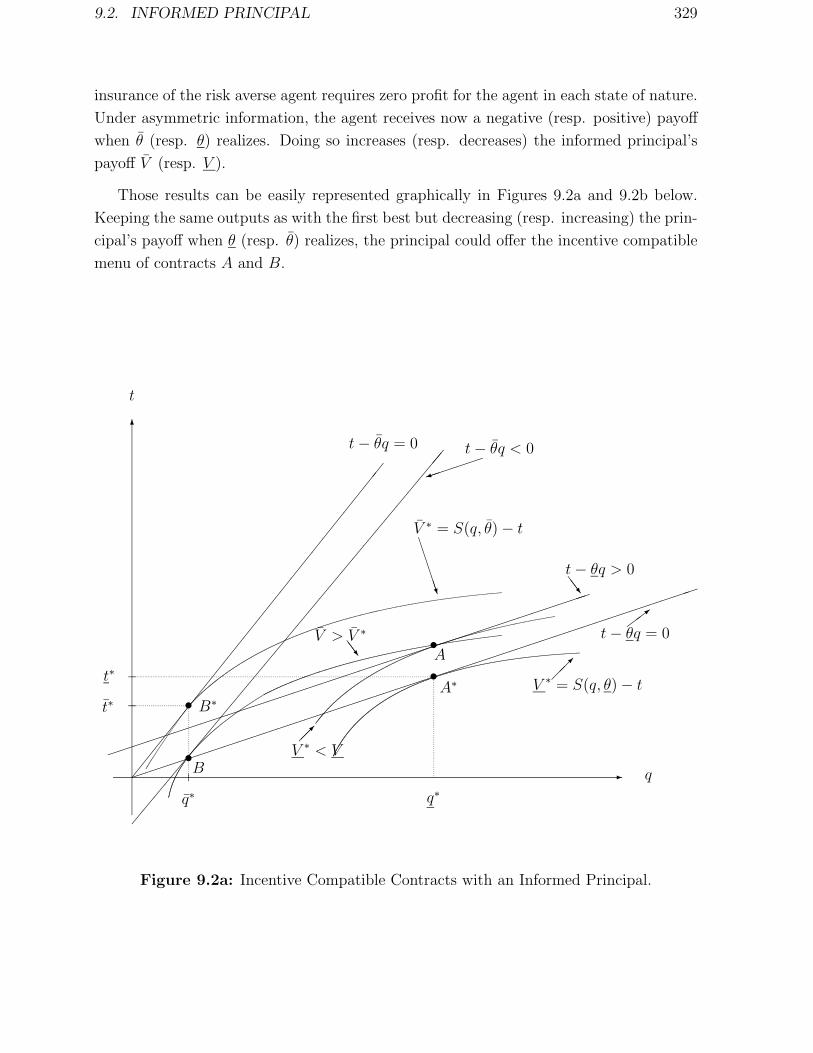
9.2. INFORMED PRINCIPAL 329
insurance of the risk averse agent requires zero profit for the agent in each state of nature.
Under asymmetric information, the agent receives now a negative (resp. positive) payoff
when θ (resp. θ) realizes. Doing so increases (resp. decreases) the informed principal’s
payoff V (resp. V ).
Those results can be easily represented graphically in Figures 9.2a and 9.2b below.
Keeping the same outputs as with the first best but decreasing (resp. increasing) the prin-
cipal’s payoff when θ (resp. θ) realizes, the principal could offer the incentive compatible
menu of contracts A and B.
-
6
t
q¿¿
¿¿
¿¿
¿¿
¿¿
¿¿
¿¿
¿¿
¿¿
¿¿
¿¿
¿¿
t− θq = 0
³³³³³³³³³³³³³³³³³³³³³³³³³³³³³³³³³³³³³³³³³³³
t∗
t∗ ••
B∗A∗
q∗ q∗
³³³³³³³³³³³³³³³³³³³³³³³³³³³³³³³³³³³³³
%%
%%
%%
%%
%%
%%
%%
%%
%%
%%
%%
%%
%%
%%%
t− θq < 0
•A
V ∗ = S(q, θ)− t¡¡µ
t− θq > 0SSw
V > V ∗SSw
³³³³³)
•B
t− θq = 0½½>
V ∗ < V¡¡µ
V ∗ = S(q, θ)− tBBBBBN
Figure 9.2a: Incentive Compatible Contracts with an Informed Principal.

330 CHAPTER 9. LIMITS AND EXTENSIONS
-
6
t
q!!!!!!!!!!!!!!!!!!!!!!!!!!!!!!!!!!!
!!!!!!!!!!!!!!!!!!!!!!!!!!!!!!!!!!!!
££££££££££££££££££££££££££
££££££££££££££££££££££££££££££
•
•B∗
•BIP
B
tIP
t∗
q∗
t− θq = 0
•AIP
qIP
•
q∗
A∗
•A
t− θq = 0
¶¶7
V IP = S(θ, q)− t@
@R
V IP = S(θ, q)− tCCCW
Figure 9.2b: Second-Best Contracts with an Informed Principal.
This menu is incentive compatible since the principal is indifferent between contracts
A and B in state θ and strictly prefers A to B in state θ. However, this menu imposes too
much risk on the agent who gets a negative payoff when θ realizes and a positive payoff
when instead θ realizes. Slightly increasing t, i.e., moving from B to BIP , while moving A
to AIP on the indifference curve of the principal in state θ through BIP decreases this risk
while still preserving incentive compatibility (see Figure 9.2.b). Reducing the risk borne
by the agent enables the principal to decrease the expected transfer to the first-order
while creating only a second-order loss since q∗ is maximizing allocative efficiency. This
distortion is optimal for the pair of contracts (AIP , BIP ).
Starting from the analysis above, it is useful to stress two important limiting cases.
Risk Neutrality: Let us assume that the agent is risk neutral. Then u′(x) = 1 for all
x and (9.11) suggests that λ = 0. Indeed, with risk neutrality, the first-best outcome
can still be implemented by the informed principal. To see that, consider the following

9.2. INFORMED PRINCIPAL 331
information rents:
V ∗ = ν(S(q∗, θ)− θq∗) + (1− ν)(S(q∗, θ)− θq∗) + (1− ν)Φ(q∗), (9.15)
V ∗ = ν(S(q∗, θ)− θq∗) + (1− ν)(S(q∗, θ)− θq∗)− νΦ(q∗). (9.16)
It is easy to check that (9.1), (9.2) and (9.5) are all satisfied by those information rents
of the principal. As a result, the principal’s incentive constraints do not conflict with the
agent’s participation constraint when contracting takes place ex ante and the agent is
risk neutral. Juxtaposing this insight with the result of Section 2.12.1, we can conclude
that ex ante contracting never entails any allocative efficiency when both agents are risk
neutral whatever the allocation of bargaining power at the ex ante contracting stage.
Infinite Risk Aversion: Let us now assume that the agent is infinitely risk averse
below zero wealth and risk neutral above. The ex ante participation constraint (9.5) is
now replaced by a pair of ex post participation constraints, one for each state of nature:
U = S(q, θ)− θq − V ≥ 0, (9.17)
U = S(q, θ)− θq − V ≥ 0. (9.18)
Obviously those two constraints are binding at the optimum of the principal’s problem.
Inserting the expression of V and V obtained when (9.17) and (9.18) are binding leads to
a reduced form problem:
(P ′) : max{(q,q)}
ν(S(q, θ)− θq) + (1− ν)(S(q, θ)− θq)
subject to
S(q, θ)− θq ≥ S(q, θ)− θq. (9.19)
(9.19) is the principal’s incentive constraint when θ realizes. It has been rewritten by
using the expressions of V and V obtained from (9.17) and (9.18).
The solution of this problem is clear. There is no output distortion when θ realizes
and again qIP = q∗. Alternatively, there is an output distortion when θ realizes. Since
(9.8) holds and since S(θ, q) − θq is decreasing over the interval [q∗, +∞[4 the incentive
constraint is satisfied for a whole interval of output q in [qIP , +∞[ where qIP < q∗ and
S(θ, q∗)− θq∗ = S(θ, qIP )− θqIP . (9.20)
4Indeed, Sq(q, θ)− θ < Sq(q, θ)− θ < 0 for q ≥ q∗ where the first inequality comes from Sqθ(q, θ) < 0and the second inequality comes from the fact that S(q, θ) − θq is strictly concave in q and maximizedfor q = q∗.

332 CHAPTER 9. LIMITS AND EXTENSIONS
Moreover, since qIP < q∗ allocative efficiency is maximized over the interval by picking
qIP .
It is worth representing this distortion graphically.
-
6
t
q¿¿
¿¿
¿¿
¿¿
¿¿
¿¿
¿¿
¿¿
¿¿
¿¿
¿¿
¿¿
t− θq = 0
³³³³³³³³³³³³³³³³³³³³³³³³³³³³³³³³³³³³³³³³³³³t− θq = 0
t∗
t∗
tIP
••
•
BIP = B∗A∗
AIP
q∗ q∗ qIP
S(q, θ)− t = V ∗A
AAK S(q, θ)− t = V ∗
Figure 9.3: First-Best and Second-Best Contracts with
an Informed Principal and an Infinitely Risk Averse Agent.
In Figure 9.3, we show that the contracts A∗ and B∗ lie on the zero-profit lines of
the agent for each possible realization of the state of nature. For those contracts, the
zero-profit lines are tangent to the principal’s indifference curves in each state of nature.
Under asymmetric information, the inefficient principal still receives the allocation B∗.Instead, the efficient principal over-consumes the good and chooses contract AIP . The
corresponding output lies at the intersection between the inefficient principal’s first-best
indifference curve and the agent’s zero profit line when θ realizes. This allocation ensures
incentive compatibility since the principal strictly prefers AIP to B∗ in state θ and is
indifferent between those two allocations in state θ. Moreover, incentive compatibility is
ensured at a minimal cost from an ex ante point of view.
Remark 1: The reader who is knowledgeable in the theory of signaling will have probably

9.2. INFORMED PRINCIPAL 333
recognized the similarity of the second-best outcome obtained above with the so-called
“least costly separating equilibrium” of signaling games. Indeed, let us consider the follow-
ing game. First, the principal learns the state of nature θ, second he chooses a “capacity of
consumption” q and third, a competitive market of sellers, the “agent,” offers the good to
the principal up to his consumption capacity. One can show that this game has different
classes of perfect Bayesian equilibria:5 pooling equilibria where the principal chooses the
same capacity in each state of nature and separating equilibria where those capacities are
different. Separating equilibria are thus revealing the private information learned by the
principal to the competitive market. We let the reader check that those latter equilibria
entail over-investment in capacity by the efficient type in order to credibly commit to
signal his type to the market.6 Moreover, the Cho-Kreps (1987) “intuitive criterion” se-
lects among those equilibria the “least-cost separating allocation” which is precisely that
obtained when the principal chooses qIP in state θ, exactly as under ex ante contracting.
In our model, the inefficiency of some equilibria of the signaling game can be overcome
by writing an ex ante contract. However, not all inefficiency disappears even in this case
because incentive compatibility must be preserved.
Remark 2: The allocative inefficiency obtained above is strongly linked to the assumption
of common values. Suppose instead that θ does not enter into the agent’s utility function
which writes as U = t − q for t − q ≥ 0, −∞ otherwise. Then, it is easy to check that
t∗ = q∗ and t = q∗ implement the first-best productions. To have inefficiency, we must
have an informational externality between the two types of principal.
The literature on informed principals is relatively thin and will be covered more
extensively in Volume III. Myerson (1983), Maskin and Tirole (1990) and (1992) were all
interested in models with ex post contracting, i.e., when the principal offers the contract
to the agent once he already knows the state of nature. These models belong thus to the
realm of signaling theory. Maskin and Tirole (1990) offered a non-cooperative analysis of
the game with private values. They showed that the principal’s private information had
no value when he is risk averse. With risk aversion, they also showed that the perfect
Bayesian equilibria of the game were obtained as Walrasian equilibria of an exchange
economy among the different types of principal. Maskin and Tirole (1992) analyzed a
game with common values and showed that the perfect Bayesian equilibria of this game
could be easily obtained as contracts giving higher payoffs to each type of principal than
what they get in the least cost separating allocation.7 Taking a cooperative perspective,
5See Fudenberg and Tirole (1991) for a definition.6The analogy with a Spencian model of the labor market is straightforward and the method of reso-
lution used in standard textbooks like, for instance, Green, Mas-Colell and Whinston (1995, Chapter 13)can be used to derive those equilibria.
7This allocation is often called the Rotschild-Stiglitz-Wilson allocation (see Rotschild and Stiglitz(1976) and Wilson (1976).

334 CHAPTER 9. LIMITS AND EXTENSIONS
Myerson (1983) showed as “inscrutability principle” arguing that the principal could al-
ways build into the mechanism itself the revelation of his type. He went on by presenting
various concepts of solution, some of them being cooperative. Stoughton and Talmor
(1990) compared the signaling and the screening distortions in a model of transfer pric-
ing. Finally, Beaudry (1991) analyzed a mixed model where the principal privately knows
the distribution of outcomes that the agent may generate by exerting a non-observable
effort.
9.3 Limits to Enforcement
In this volume, we have assumed that the judicial system is perfect and benevolent, and
consequently can enforce any contract. Implicit behind this enforcement is the use of
penalties which prevent both partners to breach the contract. We now discuss briefly a
model of imperfect contractual enforcement.
Consider the model of Section 2.12.1 with adverse selection, risk neutrality and ex ante
contracting, i.e., the principal offers a contract before the risk neutral agent discovers its
private information. We know that the first-best is then implementable. However, the ex
post utility level of the agent is negative when θ realizes. Indeed, the inefficient agent’s
payoff is U∗ = t∗ − θq∗ = −ν∆θq∗ < 0. Then, this agent may be tempted to renege on
the contract proposed by the principal to avoid this negative payoff.
Let us first assume that the judicial system is so inefficient that the principal can never
enforce a contract with such a negative payoff. Anticipating this fact, the principal reverts
to self-enforcing contracts which are such that both ex post participation constraints
U = t − θq ≥ 0 and U = t − θq ≥ 0 are satisfied. In this case, we are exactly in
the same situation as if the agent knew his private information at the time of signing the
contract. The optimal self-enforcing contract is thus identical to the contract characterized
in Section 2.7.
The expected loss LSB incurred by the principal because of the complete absence of
enforcement can be easily computed as:
LSB =(ν(S(q∗)− θq∗) + (1− ν)(S(q∗)− θq∗)
)− (
ν(S(q∗)− θq∗ −∆θqSB) + (1− ν)(S(qSB)− θqSB))
= ν∆θqSB︸ ︷︷ ︸Rent Loss
+(1− ν)((S(q∗)− θq∗)− (S(qSB)− θqSB)
)︸ ︷︷ ︸Efficiency Loss
. (9.21)
The expected loss associated with the complete absence of a judicial system enforcing
contracts is thus composed of two terms: First, the information rent needed to elicit

9.3. LIMITS TO ENFORCEMENT 335
information when the agent’s ex post participation constraints must be satisfied; and
second, the corresponding allocative inefficiency when θ realizes.
Let us now analyze the case where the judicial system can enforce any contract stipu-
lating a negative payoff with some probability p at a cost c(p). We assume that the cost
of enforcement is increasing and convex: c(0) = 0, c′(·) ≥ 0 (with the Inada conditions
c′(0) = 0 and c′(1) = +∞), and c′′(·) > 0.
A mechanism is enforcement-proof if the inefficient agent finds always optimal to
comply and prefers taking the promised rent U rather than refusing to produce. If he
refuses to comply, the Court enforces nevertheless the contract with probability p and
imposes an exogenous penalty P on the agent.8 The enforcement-proofness constraint
writes thus as:
U ≥ p(U − P ), (9.22)
or putting it differently as
U ≥ − pP
1− p. (9.23)
As in our analysis of auditing models made in Section 3.7, the monetary punishment
P can be either endogenous or exogenous. In the first case, P is bounded above by the
value of the agent’s assets ` plus the latter’s information rent:
P ≤ U + `. (9.24)
In the case of exogenous punishments, P is only bounded by the value of the agent’s
assets:
P ≤ `. (9.25)
We will focus on this latter case in what follows. When the principal chooses to
implement an enforcement-proof mechanism, he solves therefore the following program:
(P ) : max{(U ,q);(U,q)}
ν(S(q)− θq − U
)+ (1− ν)
(S(q)− θq − U − c(p)
)subject to (9.23), (9.25) and9
U ≥ U + ∆θq, (9.26)
νU + (1− ν)U ≥ 0. (9.27)8In fact, only the inefficient agent is willing to renege on the contract since the efficient agent always
gets a positive payoff. Hence, the Court and the principal know for sure the agent’s type when the latterrefuses to enforce the contract.
9We neglect the inefficient agent’s incentive constraint which is satisfied as it can be easily checked expost.

336 CHAPTER 9. LIMITS AND EXTENSIONS
First, note that the principal incurs the cost of the judicial system. Specifically, we
assume that the principal pays an amount (1 − ν)c(p) to maintain a judicial system of
quality p. Second, the principal’s objective function takes into account the fact that
the contract is always enforced on the equilibrium path when it is enforcement-proof.
Henceforth, the punishment P is only used as an out-of-equilibrium threat to force the
inefficient agent’s compliance. Of course, the maximal punishment principle already seen
in Section 3.7 still applies in this context and the constraint (9.25) is binding at the
optimum.
Remark: The reader will have noticed that the model above is somewhat similar to the
models of audit studied in Section 3.7. The only difference comes from the role played by
the probability of enforcement p. Instead of being used to relax an incentive constraint,
a greater probability of audit relaxes a participation constraint.
It is outside the scope of this section to analyze all possible regimes which may arise
at the optimum. However, note that (9.25) is binding when:
ν∆θq >p
1− p`. (9.28)
In this case, the agent’s information rents in the states of nature θ and θ are respectively
given by U = ∆θq− p1−p
` and U = − p1−p
`. Inserting those expressions into the principal’s
objective function and optimizing with respect to q and q leads to the following expressions
of the second-best outputs: qEP = q∗ and S ′(qEP ) = θ + ν1−ν
∆θ where the superscript
EP means “enforcement-proof.” These outputs are thus exactly the same as in the case
of self-enforcing contracts seen above.
Omitting terms which do not depend on p, the principal finds the optimal probability
of enforcement as a solution to the following problem:
(P ′) : max{p}
p`
1− p− (1− ν)c(p).
This objective function is strictly concave with respect to p when c(·) is sufficiently
convex. Hence, its maximand is obtained for pEP such that 0 < pEP < 1.
The judicial system commits therefore to an optimal probability of enforcement pEP
which is the unique solution to:
`
(1− ν)(1− pEP )2= c′(pEP ). (9.29)
Note also that the probability of enforcement pEP is increasing in the liability of the
agent ` when c(·) is sufficiently convex.
Of course, the pair (qEP , pEP ) is really the solution we are looking for when the con-
dition (9.28) holds for pEP defined in (9.29). In particular, this condition holds when the

9.3. LIMITS TO ENFORCEMENT 337
cost of enforcing contract is large enough and pEP is close to zero.
With the optimal enforcement-proof mechanism, the principal obtains an expected
payoff:
V EP = ν(S(q∗)− θq∗) + (1− ν)(S(qSB)− θqSB)− ν∆θqSB − (1− ν)c(pEP ) +pEP `
1− pEP.
(9.30)
Compared with the full enforcement outcome, the expected loss Le incurred by the
principal when the judicial system ensures a random enforcement of the contract writes
now as:
LEP = LSB − (1− ν)c(pEP ) +pEP `
1− pEP. (9.31)
From the assumptions made on the cost of enforcement c(·), p = 0 is always a dom-
inated choice and therefore LEP < LSB. Hence, the principal finds always optimal to
use an enforcement-proof mechanism involving the threat of some random intervention
by the judge. Because pSB is strictly positive, the principal does strictly better with an
enforcement-proof mechanism than what he can get by writing a self-enforcing contract.
Note in particular that the information rent obtained by the inefficient type remains
negative, just as in the case of full enforcement.
We can summarize this section as:
Proposition 9.2 : There is no loss of generality in using enforcement-proof contracts.
The judicial system is not used on the equilibrium path but the mere possibility that it
could be used improves ex ante contracting.
Laffont and Meleu (2000) analyzed a model similar to the one we presented
above but allowed for endogenous punishments and possibly fixed costs of enforcement.
In particular, they observed that self-enforcing contracts may be optimal because of the
fixed cost of using the judicial system. Fafchamps and Minten (1999) showed empirically
that contracts used in LDCs are designed for low exposure to the breach of contracts.
Indeed, low liabilities call for a reduction in the probability of using the judicial system.
Krasa and Villamil (2000) analyzed the issue of costly enforcement in the case of financial
contracts. They showed that, under some conditions, the optimal renegotiation-proof
financial contract is actually a debt contract with deterministic audit. This result provides
a rationalization for the assumption of deterministic contracts often made in the costly
state verification literature.10
10See Section 3.7.

338 CHAPTER 9. LIMITS AND EXTENSIONS
9.4 Dynamics and Limited Commitment
In an intertemporal framework, what is needed for the optimal dynamic contract to be
credible is not only the ability of the contractual partners to commit to a contract, but the
stronger assumption that those two contractual partners have also the ability to commit
not to renegotiate their initial agreement. The assumption that economic agents have the
ability to commit not to renegotiate is an extreme assumption about the perfection of
the judicial system. Clearly, weakening the assumption that the court is perfect implies
that, as we know in practice, it is very difficult and often impossible to commit not to
renegotiate.
Starting with Dewatripont (1986), the literature has explored the implications of this
institutional “imperfection” corresponding to the agents’ inability to commit not to rene-
gotiate. Moving away from the framework of full commitment raises numerous issues such
as how should we model the renegotiation game,11 how do agents update their beliefs dy-
namically and, finally, how can we characterize implementable allocations.
We sketch below the nature of the difficulty due to an imperfect commitment in
repeated adverse selection models. Take the two-period model of Section 8.2.1 and assume
now that the principal cannot commit not to renegotiate the long term agreement he has
signed with the agent. The agent knows that any information he might reveal in the first
period of the relationship will be fully used by the principal in the second period 2 if a
renegotiation is feasible. We assume that the principal still has all the bargaining power
at the renegotiation stage. Let us thus envision two possible classes of renegotiation-proof
contracts12 giving rise to two different classes of implementable allocations.
Separating Contracts:
Suppose that, in period 1, the agent behaves differently when θ = θ and when θ = θ
as it is requested by the full commitment optimal contract. The first period action
signals the agent’s type perfectly to the principal. The principal is therefore informed
on the agent’s type when period 2 comes. In particular, if the agent is a θ-type, the
principal would like to raise allocative efficiency in period 2 by increasing the second period
output still maintaining the second period rent which was promised in the optimal long-
term contract with full commitment to the θ-type. However, raising allocative efficiency
ex post has a drawback on the first period incentives. Indeed, the efficient agent is
no longer indifferent between telling the truth or not in the first period. Instead he
would like to lie to benefit from the higher rent promised in period 2. Raising ex post
11The reader has already seen in Chapter 6 instances of contracting environments where the allocationof bargaining power may change during the relationship. The same issue arises when one allows forrenegotiation.
12There is, in the same spirit as in the Revelation Principle, no loss for the principal to restrict himselfto renegotiation-proof contracts.

9.4. DYNAMICS AND LIMITED COMMITMENT 339
efficiency through the renegotiation procedure hardens first period incentives. Offering
a first period contract which fully separates both types facilitates information learning
in the organization and improves the value of recontracting in period 2. However, this
information learning may be quite costly for the principal from a first period point of
view since he must further compensate the efficient agent for an early revelation of his
type. Such a fully separating allocation is robust to the possibility of renegotiation, i.e., is
renegotiation-proof, if conditionally on the information learned after the choice of output
made at date 1, the principal cannot propose to the agent a Pareto-improving second
period contract.
Let us denote with a subscript i the contract offered at date i. If the first period
contract fully separates both types, the second period outputs are efficient in both states
of nature13 and are thus (with our usual notations) given by q∗ and q∗ depending on
the agent’s type. The efficient agent’s intertemporal incentive constraint which must be
satisfied to induce information revelation in period 1 writes finally as:
U ≥ U + ∆θ(q1 + δq∗), (9.32)
where ∆θq1 (resp. δ∆θq∗) is the first (resp. second) period benefit of a θ-agent from
mimicking the θ-agent.
The inefficient agent’s intertemporal participation constraint writes also as:
U ≥ 0. (9.33)
With such a separating contract, the principal promises to the efficient (resp. in-
efficient) agent that he will get a rent ∆θq∗ (resp. 0) in period 2. Given this initial
commitment, and the fact that the principal is fully informed on the agent’s type at the
renegotiation stage, the principal cannot raise further second period ex post efficiency
since it is already maximized with outputs q∗ and q∗. Hence, such a long term separating
contract is clearly renegotiation-proof.
Within the class of contracts which are fully separating and renegotiation-proof, the
principal finds the optimal one as a solution to the problem below:
(P S) :
max{(q
1,U);(q1,U)}
ν(S(q
1)− θq
1+ δ(S(q∗)− θq∗)− U
)+(1−ν)
(S(q1)− θq1 + δ(S(q∗)− θq∗)− U
)subject to (9.32) and (9.33).
We index with a superscript RPS meaning “renegotiation-proof and separating” the so-
lution to this problem.
13Indeed, renegotiation takes place under complete information and leads to an efficient outcome.

340 CHAPTER 9. LIMITS AND EXTENSIONS
We let the reader check that (9.32) and (9.33) are the only two binding constraints of
the problem above.
The optimal fully separating contract entails no allocative distortion for the efficient
type in both periods qRPS1
= q∗. On the contrary, it entails a downward distortion in the
first period only for the inefficient type, i.e., qRPS1 = qSB < q∗ = qRPS
2 where, as usual,
S ′(qSB) = θ + ν1−ν
∆θ.
Let us denote by V (q, q) the principal’s profit when he implements at minimal cost a
pair of outputs (q, q) in a one-period static relationship. We know from Chapter 2 that
the following equality holds:
V (q, q) = ν(S(q)− θq) + (1− ν)
(S(q)− θq − ν
1− ν∆θq
). (9.34)
It is easy to check that the intertemporal profit achieved with the optimal fully sepa-
rating contract can be written as:
V S = V (q∗, qSB) + δV (q∗, q∗). (9.35)
Pooling Contracts:
Suppose instead that, in period 1, the agent chooses the same behavior whatever his type
θ. Then, the principal learns nothing from the first period actions. The continuation
contract for period 2 should thus be equal to the optimal static contract conditional on
the prior beliefs (ν, 1− ν) since beliefs are unchanged. This contract is well-known from
Chapter 2. We index with a superscript RPP meaning renegotiation-proof and pooling
the optimal contract.
Fist, note that the second-period outputs qRPP and qRPP are thus defined by q∗ = qRPP
and qRPP = qSB. With a first period single contract (t, q) which induces full pooling be-
tween both types in the first period, the intertemporal incentive constraint of the efficient
agent writes then as:
U ≥ U + ∆θ(q + δqSB), (9.36)
where ∆θq (resp. δ∆θqSB) is the first (resp. second) period benefit of a θ-agent from
mimicking a θ-agent.
The principal’s problem which consists in finding the best long term contract inducing
full pooling in the first period is then:
(P P ) :
max{(q,U,U)}
ν(S(q)− θq + δ(S(q∗)− θq∗)− U
)+(1−ν)
(S(q)− θq + δ(S(qSB)− θqSB)− U
)

9.4. DYNAMICS AND LIMITED COMMITMENT 341
subject to (9.36) and (9.33).
Again, those latter two constraints are binding at the optimum and we find that
qRPP = q∗. The second period contract being the optimal static contract computed with
prior beliefs, it is obviously renegotiation-proof, i.e., optimal in period 2 given the common
knowledge information structure at that date.
The principal’s intertemporal profit with a pooling contract becomes now:
V P = V (qRPP , qRPP ) + δV (q∗, qSB). (9.37)
First note that, by definition of the optimal static contract, we have:
max(V (qRPP , qRPP ), V (q∗, q∗)
) ≤ V (q∗, qSB). (9.38)
The comparison of V P and V S is now immediate.
Proposition 9.3 : There exists δ0 > 0 such that the principal prefers to offer a separating
and renegotiation-proof contract rather than a renegotiation-proof pooling contract if and
only if 0 ≤ δ ≤ δ0. We have:
δ0 =V (q∗, qSB)− V (qRPP , qRPP )
V (q∗, qSB)− V (q∗, q∗). (9.39)
This proposition illustrates the basic trade-off faced by the principal under renego-
tiation. When the future does not count much (δ small), the principal can afford full
revelation in the first period without having too much (in discounted terms) to offer for
the second period. The separating long term contract dominates. When the future mat-
ters much more (δ large14), the principal would like to commit in a renegotiation-proof
way to offer the full commitment static solution in period 2. He can do so at almost no
cost (again in discounted terms) by offering a pooling contract in the first period since
this first period does not count too much. The pooling long term contract dominates.
Remark 1: The last proposition yields also some insights about the optimal speed of
information revelation in the hierarchy. This speed is a decreasing function of the discount
factor.
Remark 2: The previous analysis has focused on two simple classes of renegotiation-proof
mechanisms: fully separating and fully pooling contracts. More generally, it is optimal
14We consider that δ can be larger than one to capture the idea that the second period is much longerthan the first one.

342 CHAPTER 9. LIMITS AND EXTENSIONS
for the principal to offer in period 1 a menu of contracts which induces the efficient agent
to randomize between the long term contract intended for the efficient agent and the long
term contract intended for the inefficient one. The θ-agent chooses the latter contract
with probability one. Therefore, when the principal observes the first choice, he knows
that it is the efficient agent who made this choice for sure. When he observes the second
choice, the principal is still unsure of the agent’s type. Both types of agent may have
taken this contract. He must update his beliefs on the agent’s type from the equilibrium
strategies of the agent and he offers in period 2 the optimal menu of contracts conditional
on his new beliefs. For an equilibrium to hold, mixing is quite crucial. The efficient
agent must be indifferent between the first period rent he gets if he reveals his type in
period 1 and the sum of the rent he gets in period 1 by mimicking the θ-type and of the
rent he gets in period 2 by choosing its best element within the menu offered. Inducing
randomization by the θ-agent is the only way available to “indirectly commit” to leave a
rent to the θ-agent in period 2. Indeed, leaving a rent in period 2 is ex post optimal for
a principal who suffers from asymmetric information about the agent’s type.
As the reader may have guessed from the discussion above, a careful analysis of the op-
timal contract with renegotiation, requires a complex notion of equilibrium involving both
dynamic considerations and asymmetric information: the perfect Bayesian equilibrium.15
This analysis will be undertaken in Volume III.
Dewatripont (1989) analyzed long term renegotiation-proof labor contracts in
a T -period environment. The focus was on the choice between separating and pooling
mechanisms. Dewatripont (1986) and Hart and Tirole (1988) provided proofs of the
Renegotiation-Proofness Principle which allows the modeler to restrict the principal to
offer renegotiation-proof long term contracts. Hart and Tirole (1988) studied also a T pe-
riod environment with quantities traded being restricted to {0, 1}. The main achievement
of the paper was to provide an analysis of the process by which information is gradually
revealed over time. Laffont and Tirole (1990b) offered a complete analysis of the 2-period
model with randomized strategies and unrestricted quantities. Rey and Salanie (1996)
discussed the conditions under which the optimal long term contract over T periods can
be replicated by a sequence of two period short-term contracts. Bester and Strauss (1999)
have extended the Revelation Principle in this context and have shown that there is no
loss of generality in looking at first period mechanisms stipulating as many transfers and
outputs as the cardinality of the type space.
15The same holds for short-term contracts (one-period commitment).

9.5. THE HOLD-UP PROBLEM 343
9.5 The Hold-Up Problem and the Limits of Com-
mitment
9.5.1 Adverse Selection
Let us return to the mixed model of Section 7.3.3. Contrary to what we have assumed
there, we analyze now a case where the principal has no ability to commit to a contract
before the agent exerts his binary effort e to improve the probability ν(e) that θ realizes.
We denote ν(1) = ν1 and ν(0) = ν0, and ∆ν = ν1−ν0 > 0 the increase in the probability of
having an efficient type when the agent increases his effort. The timing of the contractual
game is thus the following:
- time? ??? ?
t = 0 t = 1 t = 2 t = 3 t = 4
Aexerts an effort
e which isnot observed
by P
θ is realizedOnly A
learns this piece
of information
Poffers
a contract t(q)
to A
Aaccepts or not
the contract
Achooses theproduction q
and receivesthe transfer t(q)
Figure 9.4: Timing of the Hold-Up Problem.
In the hold-up problem, the principal cannot commit to reward ex ante the agent for
his non-observable effort. Ex post (in period 2), when the principal offers the contract,
the agent’s effort has already been sunk. The motivation for this contractual setting is
that the agent and the principal can only meet each other once the agent’s investment
has already been made.
The principal having now lost his role of Stackelberg leader in the design of incentives
for effort, we must look for a Nash equilibrium between the principal and the agent. The
principal offers a contract anticipating a particular choice of effort made by the agent. The
agent chooses an effort level anticipating the contract he will receive from the principal.
Let us denote by νe the conjecture of the principal over the probability that type
θ realizes. Using the results of Chapter 2, the “best-response” of the principal is thus
characterized by an output distortion (for the inefficient type only) q(νe) which is defined
by
S ′(q(νe)) = θ +νe
1− νe
∆θ; (9.40)
and a positive information rent (for the efficient type only) given by U(νe) = ∆θq(νe).
Note that q(νe) and U(νe) are both decreasing with νe.

344 CHAPTER 9. LIMITS AND EXTENSIONS
Anticipating such a contract and more specifically the rent ∆θqe he will get when he
turns out to be efficient, the agent invests in increasing this probability according to the
following best response e = 1 if ∆ν∆θqe > ψ, e = 0 if ∆ν∆θqe < ψ, and e in [0, 1] if
∆ν∆θqe = ψ.
This yields the following characterization of the Nash equilibrium contract and effort
in this framework without any commitment.
Proposition 9.4 : Assume that the principal cannot commit to a contract before the
agent exerts effort. Then, the equilibrium allocation is characterized as follows:
• If ∆θq(ν1) > ψ∆ν
, the agent exerts a positive effort and q(ν1) is chosen by the prin-
cipal.
• If ∆θq(ν0) < ψ∆ν
, the agent does not exert any effort and q(ν0) is chosen by the
principal.
• If ∆θq(ν1) ≤ ψ∆ν≤ ∆θq(ν0), the agent randomizes between exerting effort or not with
respective probabilities ε and 1−ε. We have νe = εν1 +(1−ε)ν0 and ∆θq(νe) = ψ∆ν
.
When ψ∆ν
≥ ∆θq(ν1), under-investment occurs with respect to the case with full
commitment seen in Section 7.3.3.16 The logic underlying this result is simple. The agent
only receives a share (his information rent) of the overall surplus of production which
occurs in period 4; hence he may not have enough incentives to exert effort.
Schmidt (1996) used the under-investment problem above to build a theory of
privatization. In this theory, the cost of public ownership is the inability of the State to
reward a specific investment made at the ex ante stage by the public utility.
9.5.2 Non-verifiability
The hold-up problem may also arise in the framework of mixed models with non-verifiability
of the state θ instead of adverse selection. Still keeping the timing of Figure 9.4, θ is now
commonly learned by the agent and the principal at date 1. Suppose, as we did in Sec-
tion 6.2.1, that no contract is ever signed between t = 0 and t = 1 and that the agent
and the principal bargain ex post over the gains from trade. Taking the Nash bargain-
ing solution with equal weights to compute their final payoffs,17 we find that the agent’s
16Recall that we made there the assumption that the principal’s benefit from inducing a high effortwas large enough.
17See Section 6.2 for a model with the Nash bargaining solution.

9.5. THE HOLD-UP PROBLEM 345
ex ante expected utility writes as 12
(ν(e)W ∗ + (1− ν(e))W ∗) − ψ(e), where, as usual,
W ∗ = S(q∗) − θq∗ and W ∗ = S(q∗) − θq∗ denote the first-best surpluses in each state of
nature. Henceforth, the agent invests if and only if:
∆ν
2(W ∗ − W ∗) > ψ. (9.41)
Effort may be optimal when ∆ν(W ∗ − W ∗) > ψ, but the condition (9.41) may no
longer hold when ∆ν2
(W ∗ − W ∗) < ψ < ∆ν(W ∗ − W ∗). In this case, there is again
under-investment and the hold-up problem reappears.
Proposition 9.5 : Assume that the state of nature is nonverifiable and that the agent
has only a limited bargaining power in the negotiation over the ex post gains from trade;
then an under-investment may occur.
The intuition behind this proposition is straightforward. Since the agent only gets half
of the ex post gains from trade, he has only half of the social incentives to exert effort.
Under-provision of effort follows.
Remark: Simple solutions to this hold-up problem can nevertheless be found by the
contractual partners. First, the ex post bargaining power could be fully allocated to the
agent, making him residual claimant for the social return to investment. Of course, this
solution may not be optimal if the principal also has to invest in the relationship18 or if
the agent is risk averse since he would then bear too much risk.
Second, let us assume that the principal and the agent can agree ex ante on an ex
post allocation (t0, q0) which stipulates the status quo payoffs of both the agent and the
principal in the ex post bargaining taking place when θ has realized. This contract is
relatively simple to write since it stipulates only one transfer and an output. Moreover,
we assume that the principal keeps all the bargaining power in the ex post bargaining
stage. He must therefore solve the following problem:
(P ) : max{(q,t)}
S(q)− t
subject to
t− θq ≥ t0 − θq0 (9.42)
where (9.42) is the agent’s participation constraint which is obviously binding at the
optimum since the principal wants to reduce the agent’s transfer as much as possible.
18This kind of model requires that both the principal and the agent exert a nonverifiable investmentat the ex ante stage.

346 CHAPTER 9. LIMITS AND EXTENSIONS
Since there is complete information ex post, the efficient production levels q∗ and q∗
are chosen by the principal depending on which state of nature realizes. The agent’s
expected payoff writes thus as t0 −(ν(e)θ + (1− ν(e))θ
)q0 − ψ(e) when he exerts effort
e. The agent exerts a positive effort when q0 is fixed so that ∆ν∆θq0 = ψ. The status
quo output q0 defines therefore the agent’s marginal incentives to invest. Then, t0 can be
adjusted so that the agent’s expected utility is zero, i.e., t0 =(ν1θ + (1− ν1)θ
)q0 + ψ.
The principal’s expected payoff becomes then ν1W∗ + (1 − ν1)W
∗ − ψ, exactly as in a
world of complete contracts.
Hence, since the principal is residual claimant of the social surplus, this procedure
would also induce him to invest efficiently if he could affect the probability ν1(ep) by some
costly effort ep.
This very nice solution to the hold up problem is due to Chung (1991). Various
other solutions have been found in the incomplete contracts literature that we will analyze
in Volume III.
9.6 Limits to the Complexity of Contracts
In most of this book, we have deliberately chosen to emphasize simple models where
shocks are discretely distributed both in the case of adverse selection and moral haz-
ard. However, the analysis of Appendix 2.1 and Appendix 4.2 suggests also that optimal
contracts may have quite complex shapes in the richer case where those shocks are contin-
uously distributed. This complexity has often been viewed as a failure of contract theory
to capture the simplicity of real world contracting environments. We now illustrate in
this section how incentive theory can be reconciled with this observed simplicity provided
that the contractual environment is sufficiently structured.
9.6.1 Menu of Linear Contracts under Adverse Selection
Let us reconsider the optimal contract obtained in Appendix 2.1, in the case of a contin-
uum of types distributed according to the cumulative distribution F (·) with density f(·)on the interval [θ, θ]. Let us slightly generalize the framework of that appendix and also
assume that the agent has a production function θc(q) where c′(·) > 0 and c′′(·) > 0.
This extension is straightforward and we let it as an exercise to the reader. The optimal
second-best production levels qSB(θ) under asymmetric information are characterized by:
S ′(qSB(θ)) =
(θ +
F (θ)
f(θ)
)c′(qSB(θ)). (9.43)

9.6. LIMITS TO THE COMPLEXITY OF CONTRACTS 347
When the monotone hazard rate property ddθ
(F (θ)f(θ)
)> 0 is satisfied, the schedule of
output qSB(θ) is invertible. Let θSB(q) be its inverse function. The transfer tSB(θ) paid
to the agent is such that:
tSB(θ)− θc(qSB(θ)) =
∫ θ
θ
c(qSB(x))dx (9.44)
where the right-hand side above is θ-type’s information rent U(θ).
Instead of using the direct revelation mechanism {(tSB(θ), qSB(θ))}, the principal could
give up any communication with the agent and let him choose directly an output within
a nonlinear schedule T SB(q). This procedure is basically the reverse of the Revelation
Principle; it is sometimes called the Taxation Principle.19 To reconstruct the indirect
mechanism T SB(q) from the direct mechanism {tSB(θ), qSB(θ)} is rather easy. Indeed, we
must have T SB(q) = tSB(θSB(q)).
When he faces the nonlinear payment T SB(q), the agent replicates the same choice
of output as with the direct revelation mechanism {(tSB(θ), qSB(θ))}. Indeed, we have
T SB(q) = tSB(θSB(q))θSB(q), and thus
T SB(qSB(θ)) =tSB(θ)
qSB(θ), for any θ in [θ, θ]. (9.45)
Differentiating (9.44) with respect to θ yields immediately tSB(θ) = θc′(qSB(θ))qSB(θ).20
Inserting into (9.45) we obtain
T SB(qSB(θ)) = θc′(qSB(θ)), (9.46)
which is precisely the first-order condition of the agent’s problem when he chooses an
output within the nonlinear schedule T SB(·).That the agent’s choice can be implemented with a nonlinear payment T SB(·) is im-
portant. However, in practice, one observes quite often menus of linear contracts to choose
from. This is for instance the case for the relationship between regulatory agencies and
regulated firms or the relationship between a buyer and a seller.21
To obtain an implementation of the second-best outcome with a menu of linear con-
tracts requires to be able to replace the nonlinear schedule T SB(q) by the menu of its
tangents. The slope of the tangent at a given point qSB(θ) is the same as that of T SB(q)
19See Guesnerie (1995) and Rochet (1985).20The reader will have recognized the first-order condition associated with the fact that telling the truth
is an optimal strategy for the agent with type θ when he faces the truthful direct revelation mechanism{(tSB(θ), qSB(θ))}.
21Wilson (1993) argues that a menu with very few linear contracts can almost replicate the performancesof a nonlinear prices.

348 CHAPTER 9. LIMITS AND EXTENSIONS
at this point. Hence, the type θ agent’s marginal incentives to deviate away from qSB(θ)
are the same with both mechanisms. Moreover the tangent has also the same value as
T SB(q) at qSB(θ). Hence, the nonlinear schedule T SB(·) and its menu of tangents provide
the agent with the same information rent. This equivalence is nevertheless only possible
when T SB(q) is in fact convex. Figure 9.5 below represents this case.
-
6
½½
½½
½½
½½
½½
½½
½½½
··
··
··
··
··
··
···
@@I
Indifference curve of a θ-agent
t− θc(q) = U(θ)
T SB(q)
q
t
•
qSB(θ)
tSB(θ)S
SSSo
6
Tangents
PPPPPq
Figure 9.5: Convexity of the Nonlinear Schedule T SB(q).
Let us thus derive the conditions ensuring this convexity. Differentiating (9.46), we
obtain:
T SB(qSB(θ)) =c′(qSB(θ))
qSB(θ)+ θc′′(qSB(θ)), (9.47)
where qSB(θ) is obtained by differentiating (9.43) with respect to θ and we find:
qSB(θ)
c′(qSB(θ))=
1 + ddθ
(F (θ)f(θ)
)S ′′(qSB(θ))− c′′(qSB(θ))S′(qSB(θ))
c′(qSB(θ))
. (9.48)

9.6. LIMITS TO THE COMPLEXITY OF CONTRACTS 349
Inserting this latter expression into (9.47), we get:
T SB(qSB(θ)) = c′′(qSB(θ))
θ +
S′′(qSB(θ))c′′(qSB(θ))
−(θ + F (θ)
f(θ)
)1 + d
dθ
(F (θ)f(θ)
)
=c′′(qSB(θ))(
1 + ddθ
(F (θ)f(θ)
)) (θ
d
dθ
(F (θ)
f(θ)
)− F (θ)
f(θ)+
S ′′(qSB(θ))
c′′(qSB(θ))
). (9.49)
We obtain immediately:
Proposition 9.6 Assume that F (θ)θf(θ)
is increasing with θ and that S ′′(q) = 0 for all q.
Then, T SB(·) is convex and can be implemented with the menu of its tangents.
Indeed, let us now consider the menu of tangents to T SB(·). The equation of the
tangent T (·, q0) to T SB(·) at a point q0 can be obtained as:
T (q, q0) = T SB(q0) + T SB′(q0)(q − q0). (9.50)
Facing the family {T (·, q0)}, the agent has now to choose which tangent is its most
preferred one and what output to produce according to this contract. The agent solves
therefore:
(P ) : max{(q,q0)}
T (q, q0)− θc(q).
The first-order conditions for this problem are respectively:
T SB(q0) = θc′(q), (9.51)
and
T SB(q0)(q − q0) = 0. (9.52)
If these necessary conditions are also sufficient, the agent with type θ chooses q = q0 =
qSB(θ). Sufficiency of (9.51) and (9.52) is guaranteed when T (q, q0)− θc(q) is concave in
(q, q0). Computing the corresponding Hessian H of second-order derivatives at the point
(qSB(θ), qSB(θ)) yields:
H =
(−θc′′(qSB(θ)) T SB(qSB(θ))
T SB(qSB(θ) T SB(qSB(θ))
). (9.53)
This Hessian is strictly definite negative when T SB(qSB(θ)) > 0 (i.e., if T SB(·) is
convex as already assumed) and T SB(qSB(θ))(θc′′(qSB(θ))− T SB(qSB(θ))
)> 0, but the
latter condition is satisfied as it can be easily seen by using (9.49).

350 CHAPTER 9. LIMITS AND EXTENSIONS
Remark: Note that if the principal observes only a random signal of q, say q + ε,
where ε is a random variable with zero mean (E(ε) = 0), the menu of linear contracts
still implements the same allocation. Indeed, the random variable ε disappears in the
incentive problem of the agent by the linearity of the expectation operator. Hence, the
menu of linear contracts is robust to the addition of some noise.
The implementation of the optimal contract with the menu of its tangents has
been extensively used in the field of regulation by Laffont and Tirole (1986) and (1993).
Caillaud, Guesnerie and Rey (1992) survey various extensions of these results and in
particular its robustness when the observation of production is noisy.
9.6.2 Linear Sharing Rules and Moral Hazard
Moral hazard environments can also have enough structure to let the linearity of contracts
emerge at the optimum. To see that, we now consider a twice repeated version of the
model of Section 5.4.2 where we neglect discounting. The agent has thus a utility function
U = u(t−ψ(e)) which is defined over monetary gains and the disutility of effort is counted
in monetary terms. We assume constant risk aversion so that u(x) = −exp(−rx) for some
r > 0. We denote by qi the outcome of the stochastic production function in period i.
These realizations are independently distributed over time. In each period, the agent can
exert a binary effort ei with a monetary cost ψi.
We assume that only the whole history of outputs can be used by the principal to
remunerate the agent. Given an history (q1, q2), the agent receives therefore a transfer
t(q1, q2) only in period 3 (see Figure 9.6 for a timing of the game after the offer of the
contract by the principal and its acceptance by the agent). Because there are two possible
outputs in each period, the number of possible histories and thus the number of final
transfers t(q1, q2) is 2× 2 = 4.
- time? ??? ?
t = 0, 5 t = 1 t = 1, 5 t = 2 t = 3
Aexerts effort e1
The first periodoutput q1
is realized
Aexerts effort e2
The secondperiod outputq2 is realized
The paymentt(q1, q2)
is madeto A
Figure 9.6: Timing of the Contractual Game.

9.6. LIMITS TO THE COMPLEXITY OF CONTRACTS 351
The logic underlying this model is that the principal can only incentivize the agent at
the end of the working period, but the agent has to choose an effort in each subperiod.22
Let us denote by U1 the agent’s value function from period 1 on, i.e., his expected
payoff if he exerts a positive effort in each period. We have:
U1 = E(q1,q2)
(u(t(q1, q2)− 2ψ)) , (9.54)
where E(q1,q2)
(·) denotes the expectation operator with respect to the distribution of histories
induced by the agent exerting a high effort in both periods. Note that the agent’s disutility
of effort being counted as a monetary term, one must subtract the total cost of efforts
along the whole history to evaluate the net monetary gain of the agent.
Using that u(x) = −exp(−rx) and the Law of Iterated Expectations, we obtain:
U1 = exp(−rψ)Eq1
(U2(q1)), (9.55)
where U2(q1) = Eq2
(u(t(q1, q2)− ψ)) is actually the agent’s value function from exerting a
positive effort in period 2 following a first period output q1.
Using the certainty equivalents (denoted by w2(q1)) of the random continuation mon-
etary gains t(q1, q2)− ψ, we can in fact rewrite U2(q1) = u(w2(q1)). Hence, inserting into
(9.56), we obtain U1 = Eq1
(u(w2(q1)− ψ)).
Inducing effort in period 1 requires that the following incentive constraint be satisfied:
U1 = −π1exp(−r(w2(q)− ψ))− (1− π1)exp(−r(w2(q)− ψ))
≥ −π0exp(−rw2(q))− (1− π0)exp(−rw2(q)). (9.56)
Similarly, inducing participation from period 1 on requires that the agent gets more
utility than by refusing to work and obtaining a zero wealth certainty equivalent. Hence,
the agent’s participation constraint writes as:
U1 ≥ −1. (9.57)
From the analysis of Section 5.4.2, the pair of certainty equivalents {(w2(q), w2(q))}belongs to the set of incentive feasible transfer pairs {(t, t)} inducing effort and partici-
pation with the agent being given a zero wealth outside opportunity in the static model
of Section 5.4.2.
Let us denote by F (0) the set of incentive feasible transfers defined by constraints
(9.56) and (9.58). We have: w2(q) = t1 and w2(q) = t1 for some pair (t1, t1) which
belongs to F (0).22Note the difference with the repeated moral hazard problem of Section 8.4 where a monetary transfer
is also given at the end of date 1, once the first period output has already been observed.

352 CHAPTER 9. LIMITS AND EXTENSIONS
Let us now move to period 2. In period 2, following a first period output q1, the
agent knows that he will receive the certainty equivalent w2(q1). Hence, the following
participation constraint is satisfied U2(q1) = −exp(−rw2(q1)). To induce effort in period
2 following a first period output q1, it must be that the following incentive constraints
(which are dependent on q1) are also satisfied:
U2(q1) = −π1exp(−r(t(q1, q)− ψ))− (1− π1)exp(−r(t(q1, q)− ψ))
≥ −π0exp(−rt(q1, q))− (1− π0)exp(−rt(q1, q)). (9.58)
Immediate observation shows that the pair of transfers {(t(q1, q), t(q1, q))}must belong
to the set of incentive feasible transfers inducing effort and participation in the static
model of Section 5.4.2 when the agent has an outside opportunity leaving him a wealth
certainty equivalent w2(q1).
From Remark 2, in Section 5.4.2, we know that we can write those transfers as t(q1, q) =
w2(q1)+ t2, and t(q1, q) = w2(q1)+t2, where the pair {(t2, t2)} belongs, as {(w2(q), w2(q))},to F (0). Henceforth, the overall transfers t(q1, q2) is the sum of two contracts belonging
to F (0). This property constitutes thus a significant reduction of the space of available
contracts.
Using the fact that shocks in each period are independently distributed, the principal’s
problem becomes now:
(P ) :
max{(t1,t1);(t2,t2)}
π21(2S− t1− t2)+π1(1−π1)(2S +2S− t1− t1− t2− t2)+(1−π1)
2(2S− t1− t2)
subject to {(ti, ti)} in F (0) for i = 1, 2.
It is straightforward to see that the optimal solution to this problem is the twice
replica of the solution (tSB, tSB) to the static problem discussed in Section 5.4.2. We
obtain immediately the linearity of the optimal schedule.
Proposition 9.7 : The optimal sharing rule tSB(q1, q2) is linear in the number of suc-
cesses or failures of the production process. We have: tSB(q, q) = 2tSB, tSB(q, q) =
tSB(q, q) = tSB + tSB, and tSB(q, q) = 2tSB.
This result obviously generalizes to T ≥ 2 periods and more than two outcomes.
Understanding this linearity result requires to come back to the main features of the
solution to the static problem of Section 5.4.2. The CARA specification for the agent’s
utility function implies the absence of any wealth effect. The wage as well as the cost of
effort in period 1 (which is counted in monetary terms) are sunk from the point of view of

9.6. LIMITS TO THE COMPLEXITY OF CONTRACTS 353
date 2 and have no impact on the incentive pressure which is needed at this date to induce
effort. This incentive pressure is exactly the same as in a static one-shot moral hazard
problem. Therefore, the principal views periods 1 and 2 as equivalent both in terms of the
stochastic processes generating output in each period and the incentive pressures needed
to induce effort. The principal just offers the same contract in each period and the overall
sharing rule based only on the whole history of outputs up to date 2 is linear in the
number of successes and failures.
Assume now that there are T ≥ 2 periods. Then, following the same logic as above, the
transfer associated with n successes and T−n failures only depends on the total production
and not on the dates at which those successes and failures take place. More precisely,
denoting by tSB(·) the common value of these transfers we have tSB(nq + (T − n)q) =
ntSB + (T −n)tSB where n is the number of successes. Denoting also by X the aggregate
output in the T -Bernoulli trials where, at each date, q is obtained with probability π1 and
q is obtained with probability 1− π1. We have X = nq + (T − n)q, and
tSB(X) = T
(tSB − q
(tSB − tSB
q − q
))︸ ︷︷ ︸
Fixed Fee
+
(tSB − tSB
q − q
)︸ ︷︷ ︸
Marginal Incentives
X. (9.59)
This relationship shows that the sharing rule between the principal and the agent is
linear in X. However, in the analysis above, the fixed fee in (9.59) becomes infinitely
large as T goes to infinity. Holmstrom and Milgrom (1987) solved this difficulty by using
a continuous time model where the agent controls in each period the drift of a Brownian
process. Typically, on an infinitesimal interval of time [t, t + dt], the aggregate output
q(t) up to date t is such that q(t + dt) − q(t) − edt is the sum of dt independently and
identically distributed random variables with mean zero. For a uni-dimensional Brownian
motion, we have thus:
dq = edt + σ2dB, (9.60)
where B is a uni-dimensional Brownian motion with unit variance and e is the agent’s
effort on the interval [t, t + dt].
In the continuous time model above, the principal can only use the overall aggregate
output q(1) = q at the end of a [0, 1] interval of time to incentivize the agent. Note
that (9.60) holds on all intervals [t, t + dt] and that the principal offers the same in-
centive pressure on each of those intervals so that effort is constant over time. Hence,
the aggregate output q(1) is a normal variable with mean e and variance σ2. When
the principal offers a linear contract t(q) = a + bq, the agent’s final wealth is also a
normal variable with mean a + be and variance b2σ2. Because the agent has constant
relative risk aversion, his certainty equivalent wealth we is thus such that exp(−rwe) =

354 CHAPTER 9. LIMITS AND EXTENSIONS
∫ +∞−∞ exp(−r(a+ bq−ψ(e)))
exp
(− (q−e)2
2σ2
)√
2πσ2dq, where
exp
(− (q−e)2
2σ2
)√
2πσ2is the density of the normal
distribution with mean e and variance σ2. We easily find that:
we = a + be− ψ(e)− rb2σ2
2. (9.61)
When the agent’s disutility of effort is quadratic, i.e., ψ(e) = e2
2, the sufficient and
necessary condition for the optimal choice of effort is e = b. The fixed fee a can be set so
that the agent’s certainty equivalent wealth is zero: a = (rσ2 − 1) e2
2.
The risk neutral principal’s expected payoff can be computed as:
∫ +∞
−∞(q − t(q))
exp(− (q−e)2
2σ2
)√
2πσ2dq = (1− b)e− a. (9.62)
The principal’s problem writes thus in a reduced form as follows:
(P ) : max{b,a,e}
(1− b)e− a
subject to
b = e and a = (rσ2 − 1)e2
2.
Replacing b and a by their values as functions of e, the principal’s problem becomes:
(P ′) : maxe
e− e2
2(1 + rσ2).
Optimizing, we find easily the second-best effort eSB:
eSB =1
1 + rσ2< 1 = eFB. (9.63)
It is interesting to note that, as the index of absolute risk aversion increases, the
second best effort is further distorted downwards. Similarly, as the output becomes a less
informative measure of the agent’s effort, i.e., as σ2 increases, this effort is also reduced.
These insights were already highlighted by our basic model of Chapter 4.
The Holmstrom and Milgrom (1987) model can be extended to the case of a
multi-dimensional Brownian process corresponding to the case where the agent’s output
is multi-dimensional. Schattler and Sung (1993) showed that a time-dependent technol-
ogy calls for the optimal contract to be nonlinear. Sung (1995) showed that the optimal
contract can still be linear when the agent controls the variance of the stochastic pro-
cess. Hellwig and Schmidt (1997) proposed further links between the discrete and the

9.7. LIMITS IN THE ACTION SPACE 355
continuous time model. Hellwig (1997) generalized the linearity result to the case of
mean-variance preferences. Lastly, Bolton and Harris (1997) generalized the Brownian
motion. Diamond (1998) proposed a static model with limited liability, risk neutrality
and three possible outcomes; linearity emerges because the agent has a rich set of choices
in the distribution of these outcomes.
9.7 Limits in the Action Space
Let us now come back to an adverse selection context. Our goal in this section is to
understand how one can possibly endogenize the action space used to contract with the
agent.
9.7.1 Extending the Action Space
We start with a highly stylized model of procurement between a principal (the buyer) and
an agent (the seller). We assume that the agent’s marginal cost θ belongs to Θ = {θ, θ}with respective probabilities ν and 1 − ν. Let us also suppose that the principal desires
only one unit of the good and has a valuation S for this unit. In this setting, the only
screening variable available is the set of types with whom he wants to contract. If the
price of the unit is θ, only the efficient agent produces and the principal gets ν(S − θ).
If the price is instead θ, both types of agent produce and the principal gets instead
ν(S − θ) + (1 − ν)(S − θ) − ν∆θ. Having both types producing is thus optimal when
ν(S − θ) < ν(S − θ) + (1− ν)(S − θ)− ν∆θ, i.e., when
S − θ >ν
1− ν∆θ. (9.64)
When (9.64) holds, there is no screening between both types.23
Let us now consider the case where the seller can incur some cost c(s, θ) to credibly
signal his type θ to the principal. We assume that c(s, θ) ≥ 0 with c(0, θ) = 0, cθss(s, θ) >
0, css(s, θ) > 0 and cθs(s, θ) < 0. Moreover, we assume that the Inada conditions cs(0, θ) =
cs(0, θ) = 0 both hold. The Spence-Mirrlees condition cθs(θ, s) < 0 means that the efficient
agent finds easier to signal his type than the inefficient one. In a Spencian tradition,24
one can think of this signal as a quality investment.
This signaling stage can be incorporated into the contract which stipulates a transfer
t(θ) and a signal s(θ) as a function of the agent’s announcement on his type θ. A direct
23The reader will have recognized a condition similar to the one obtained in Section 2.7.3 when weanalyze the issue of shut-down.
24See Spence (1973) and (1974).

356 CHAPTER 9. LIMITS AND EXTENSIONS
revelation mechanism is thus a pair {(t, s); (t, s)} which satisfies the following incentive
constraints
U = t− θ − c(s, θ) ≥ U + ∆θ + c(s, θ)− c(s, θ), (9.65)
U = t− θ − c(s, θ) ≥ U −∆θ + c(s, θ)− c(s, θ), (9.66)
and the standard participation constraints
U ≥ 0, (9.67)
U ≥ 0. (9.68)
By adding the incentive constraints (9.65), and (9.66), we get:
c(s, θ)− c(s, θ) ≥ c(s, θ)− c(s, θ), (9.69)
which can only be satisfied when s ≥ s since the Spence-Mirrlees property cθs < 0 holds.
Note this property also implies that any positive signal made by the inefficient type relaxes
the incentive constraint (9.65) because c(s, θ)− c(s, θ) < 0 when s > 0.
In general, the fact that cθs < 0 may create countervailing incentives. Let us focus
on the case where ∆θ > c(s, θ)− c(s, θ) so that θ remains the “efficient type” and (9.65)
remains the binding incentive constraint when the signal is added. In this case, the
principal’s problem becomes
(P ) : max{(s,U);(s,U)}
ν(S − θ − c(s, θ)− U) + (1− ν)(S − θ − c(s, θ)− U),
subject to (9.65) and (9.67).
Those two constraints are binding at the optimum and the principal’s problem rewrites
as:
(P ′) : max{s,s}
ν(S − θ − c(s, θ)− (c(s, θ)− c(s, θ)
)+ (1− ν)(S − θ − c(s, θ)).
Direct optimization of this strictly concave problem yields:
cs(sSB, θ) = 0, (9.70)
and
cs(sSB, θ) =
−ν
1− ν
(cs(s
SB, θ)− cs(sSB, θ)
)> 0. (9.71)
Hence, we have sSB = 0 and the most efficient type does not send any signal. However,
and more interestingly the inefficient type is induced to send a positive signal sSB > 0.

9.7. LIMITS IN THE ACTION SPACE 357
This signal relaxes the efficient type’s incentive constraint and allows the principal to
recover some screening ability since now both types choose different allocations.
Of course, inducing such a signal is costly for the principal. Starting from a setting
where the principal would contract only with the efficient agent in the absence of any
signal, the principal wants to use the costly signaling device as a new contracting tool
only when it improves his expected payoff, i.e., when the following condition holds:
ν(S − θ) < ν(S − θ)− ν∆θ
+(1− ν)
(S − θ − c(sSB, θ)− ν
1− ν(c(sSB, θ)− c(sSB, θ))
), (9.72)
i.e., when,
S − θ > c(sSB, θ) +ν
1− ν
(c(sSB, θ)− c(sSB, θ)
)+
ν
1− ν∆θ. (9.73)
It is worth noting that the right-hand side of (9.73) is smaller than the right-hand side
of (9.64). Hence, screening becomes easier when the agent has at his disposal a signaling
technology. By creating a new action whose cost for the agent is correlated with his type,
the principal can extend the space of mechanisms and makes it easier to elicit the agent’s
types. Moreover, allocative efficiency is also improved because now trade occurs with
both types.
Spence (1974) was the first to use this idea to elicit agents’ productivities from
their education level in his signaling theory. Maggi and Rodriguez-Clare (1995b) present a
model which is closely related to the one above. In their model, the principal can observe
on top of output a noisy signal θ + s on the agent’s marginal cost. The agent manipulates
this observable by playing on the noise s at a cost. Countervailing incentives may arise
from the fact that the Spence-Mirrlees conditions may no longer be satisfied.
9.7.2 Costly Action Space
When a principal-agent problem is defined, some variables are assumed to be verifiable
and contracts can be conditioned on those variables. For example, in our canonical models
of Chapter 2 and 4 it is assumed that the production level is contractible because it is
observable and verifiable by a Court of Justice. However, observability and verifiability
are generally costly and one may have the choice of observing and verifying more or less
variables. In our basic adverse selection model, we have potentially two observables, the
production level q and the ex post cost C = C(q, θ). Suppose that there is a fixed cost of
observing either q or C. If both C and q are observed by the principal, he can perfectly
infer the value of θ and achieve the first-best. This outcome is assumed to be too costly
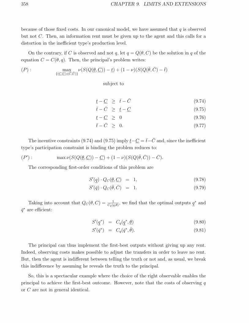
358 CHAPTER 9. LIMITS AND EXTENSIONS
because of those fixed costs. In our canonical model, we have assumed that q is observed
but not C. Then, an information rent must be given up to the agent and this calls for a
distortion in the inefficient type’s production level.
On the contrary, if C is observed and not q, let q = Q(θ, C) be the solution in q of the
equation C = C(θ, q). Then, the principal’s problem writes:
(P ) : max{(C,U);(C,U)}
ν(S(Q(θ, C))− t) + (1− ν)(S(Q(θ, C)− t)
subject to
t− C ≥ t− C (9.74)
t− C ≥ t− C (9.75)
t− C ≥ 0 (9.76)
t− C ≥ 0. (9.77)
The incentive constraints (9.74) and (9.75) imply t−C = t−C and, since the inefficient
type’s participation constraint is binding the problem reduces to:
(P ′) : max ν(S(Q(θ, C))− C) + (1− ν)(S(Q(θ, C))− C).
The corresponding first-order conditions of this problem are
S ′(q) ·QC(θ, C) = 1, (9.78)
S ′(q) ·QC(θ, C) = 1. (9.79)
Taking into account that QC(θ, C) = 1Cq(q,θ)
, we find that the optimal outputs q∗ and
q∗ are efficient:
S ′(q∗) = Cq(q∗, θ) (9.80)
S ′(q∗) = Cq(q∗, θ). (9.81)
The principal can thus implement the first-best outputs without giving up any rent.
Indeed, observing costs makes possible to adjust the transfers in order to leave no rent.
But, then the agent is indifferent between telling the truth or not and, as usual, we break
this indifference by assuming he reveals the truth to the principal.
So, this is a spectacular example where the choice of the right observable enables the
principal to achieve the first-best outcome. However, note that the costs of observing q
or C are not in general identical.

9.8. LIMITS TO RATIONAL BEHAVIOR 359
The literature has studied more generally the comparison of regulation by the
output or regulation by the input (see Maskin and Riley (1985), Crampes (1986), Khalil
and Lawarree (1995)). The levels of information rent are affected by the choice of the
contractible variables which must be optimized at the time of contracting.
9.8 Limits to Rational Behavior
Even though incentive theory has been developed under the standard assumption that all
players are rational, it can take into account whatever bounded rationality assumption
one may wish to choose. However, there is an infinity of possible theories of bounded
rationality and, in each case, the modeler must derive specific optimal contracts. Let
us consider a few examples which allows the modeler to introduce bounded rationality
without perturbing too much the basic lessons of incentive theory.
9.8.1 Trembling-Hand Behavior
Let us come back to the canonical model of Chapter 2. We will assume that the agent is
ex ante rational when he accepts the contract but makes a mistake with some probability
when he chooses the contract ex post. Ex ante rationality implies that the agent antici-
pates the impact of these future errors on his expected utility at the time of acceptance.
This possibility of an ex post irrational behavior only matters for the efficient type
when the size of the mistakes is small enough. Indeed, recall that, in the standard solution
to Chapter 2, only the efficient type is indifferent between taking his contract and that of
the inefficient type. The latter agent strictly prefers his contract and will continue to do
so as long as mistakes are small enough.
Let us denote by ε the error term in the efficient agent’s choice. The latter agent
chooses the contract (t, q) when:
U ≥ U + ∆θq + ε, (9.82)
i.e., with probability G(U − U −∆θq) where G(·) is the cumulative distribution of ε on
some centered interval [−ε, ε]. g(·) denotes the density of this random variable. Moreover,
we will assume that the monotone hazard rate property ddε
(G(ε)g(ε
)> 0 is satisfied. When
ε ¿ ∆θq, the inefficient agent does not make any error and chooses the right contract
with probability one. His acceptance is thus ensured when:
U ≥ 0.25 (9.83)

360 CHAPTER 9. LIMITS AND EXTENSIONS
The principal problem becomes then:
(P ) : max{(U ,q);(U,q)}
νG(U−U−∆θq)(S(q)−θq−U)+(1− νG(U − U −∆θq)
)(S(q)−θq−U).
subject to (9.83).
Introducing the slack ε in the efficient type’s incentive constraint, this problem rewrites
as:
(P ′) : max{(ε,q,q)}
νG(ε)(S(q)− θq −∆θq − ε) + (1− νG(ε))(S(q)− θq),
since (9.83) is necessarily binding at the optimum.
We index the optimal contract by a superscript BR meaning “bounded rationality”.
Proposition 9.8 : With a trembling-hand behavior, the optimal contract entails no out-
put distortion for the efficient type, qBR = q∗, and a downward distortion for the inefficient
type, qBR < q∗, such that:
S ′(qBR) = θ +νG(εBR)
1− νG(εBR)∆θ, (9.84)
where εBR > 0 is given by:
S(q∗)− θq∗ − (S(qBR)− θqBR) = εBR +G(εBR)
g(εBR)
(S(q∗)− θq∗ − (S(qBR)− θqBR)
).
(9.85)
Because qBR < q∗, the left-hand side of (9.85) is strictly positive. This left-hand side is
the difference between the first-best surplus and what would be obtained, had the efficient
agent made a mistake and taken the contract of an inefficient one. Since G(·) satisfies the
monotone hazard property, εBR is thus necessarily positive. Moreover, since G(εBR) < 1,
everything happens as if the efficient type was less likely. The rent differential ∆θq given
up to the efficient agent is less costly than in a model with no mistake. Hence qBR > qSB
and the output distortion is less important than without mistake.
Remark: The reader will have recognized the similarity of this section with the model
of Section 3.5. There, mistakes did not impact on the efficient type’s incentive constraint
but instead on the inefficient type’s participation constraint.
25The efficient agent’s participation constraint is instead
G(U − U −∆θq)U + (1−G(U − U −∆θq)(U + ∆θq) ≥ 0.
Again, when ε is small enough this participation constraint is strictly satisfied and can be omitted in theanalysis.

9.8. LIMITS TO RATIONAL BEHAVIOR 361
9.8.2 Satisficing Behavior
Consider a three type example along the lines of Section 9.4 with a general cost function
C(q, θ). The incentive constraints of each type write respectively as:
t− C(q, θ) ≥ t− C(q, θ) (9.86)
≥ t− C(q, θ) (9.87)
t− C(q, θ) ≥ t− C(q, θ) (9.88)
≥ t− C(q, θ) (9.89)
t− C(q, θ) ≥ t− C(q, θ) (9.90)
≥ t− C(q, θ). (9.91)
Suppose that the agent has a satisficing behavior and only looks at the nearby contracts
which are ordered as{(t, q); (t, q); (t, q)
}. Starting from an initial contract choice which
may be suboptimal, the agent moves to another contract choice if the nearby contract
yields a higher payoff.
Then, it is immediate to see that, if the Spence-Mirrlees condition is satisfied, the agent
will discover the optimal contract for him, and neglecting temporary misallocations, the
theory can proceed as if the agent was rational.26 Indeed, whatever his initial choice in
the menu, he will move in the right direction in this set.
For example, let us take the case where C(q, θ) = θq. If the agent has type θ and starts
from the contract (t, q), he moves then to (t, q) if and only if t− θq ≥ t− θq, which can be
rewritten t− θq ≥ t− θq + ∆θ(q− q). This last inequality holds since both q ≤ q and the
θ-incentive compatibility t− θq ≥ t− θq are satisfied. In a second step of the tatonnement
process, the θ-agent will move to contract (t, q) since by the incentive compatibility of the
contract, the following inequality t− θq ≥ t− θq holds.
However, if the Spence-Mirrlees condition is not satisfied, the agent may get stuck
at a non-optimal contract at some point in the tatonnement process. The principal
might then want to take into account those potential inefficiencies (which depend on the
starting choices) in his structuring of a menu. As an extreme case he might choose a single
bunching contract which gives up screening but avoids these temporaries inefficiencies.
There are many examples where an approach taking into account the agent’s bounded
rationality could be fruitful. An obvious case is when the choice is made by a group of
agents (a family, a firm or an organization) which does not reach an efficient collective
decision mechanism.
26We assume here for simplicity that the principal cannot change the menu of contracts he offeredduring the discrete-time “tatonnement” of the agent.

362 CHAPTER 9. LIMITS AND EXTENSIONS
9.8.3 Costly Communication and Complexity
The complexity of information places some limits on the possibility of its full commu-
nication and utilization. Costs of transmission, storage, and information processing are
among the factors that could cause a principal to limit the potential for information flows
between his agent and himself.
Little analysis of the interaction of incentive and communication constraints
exists (see however Green and Laffont (1986b), (1986a) and (1987).) Various papers
introduce explicitly the cost of including multiple contingencies in contracts (see Dye
(1985), Allen and Gale (1992) and Anderlini and Felli (2000) for a recent synthesis).
9.9 Endogenous Information Structures
One often heard criticism of incentive theory is that it takes information structures as
given. A more complete view of organizational design should account for the endogeneity
of these information structures. To investigate these new issues, we assume now that the
agent does not know his type a priori but can decide or not to acquire information about
his type at a cost c. Results depend finely on the precise extensive form of the game
representing the sequence of events and, in particular, when information is acquired. We
consider here the following timing (see Figure 9.7 below):
- time? ? ? ? ? ?
t = 1 t = 2 t = 3 t = 4 t = 5 t = 6
Natureselects θ
P offers acontract
{(t, q); (t, q)}
Aaccepts
or notthe contract
Achoosesor not
to learnhis type θ
The type θ
is learnedby A if
he has paid thelearning cost
Otherwise nothing
is learned
The contractis executed
Figure 9.7: Timing of the Contractual Game with Endogenous Information Structures.
The principal can decide to offer contracts which induce or not information gathering
by the agent, at a strictly positive cost c.
If the principal was not delegating the tasks of productions and information gathering,
he would choose to invest in information gathering when:
ν(S(q∗)− θq∗) + (1− ν)(S(q∗)− θq∗)− c ≥ maxq{S(q)− E(θ)q}, (9.92)

9.9. ENDOGENOUS INFORMATION STRUCTURES 363
where E(θ) = νθ + (1− ν)θ.
To implement this outcome with the delegation, the principal can offer a nonlinear
schedule t(q) = S(q)− T . With such a schedule, the agent is made residual claimant for
the hierarchy’s profit. When choosing of being informed, the agent would q∗ and q∗ in
both states of nature. Information gathering would thus occurs whenever:
ν(S(q∗)− θq∗) + (1− ν)(S(q∗)− θq∗)− T − c ≥ maxq{S(q)− E(θ)q} − T,
which is equivalent to (9.92).
Finally, when (9.92) holds, the principal fixes T to reap all ex ante gains from trade
and T = ν(S(q∗)− θq∗) + (1− ν)(S(q∗)− θq∗)− c. Otherwise, T = S(q)− E(θ)q where
S ′(q) = E(θ).
Cremer, Khalil and Rochet (1999) offered a similar analysis when the agent
accepts or rejects the contract after the information gathering stage and there is a con-
tinuum of possible types. Kessler (1998) analyzed a similar model with only two types.
Essentially, the upward/downward distortions for c small occur now with respect to the
optimal second-best contract rather than the first-best contract (participation constraints
are written at the ex post stage rather than at the ex ante stage). Lewis and Sappington
(1991), (1993), (1997) and Cremer and Khalil (1992) presented models where information
gathering takes place before signing the contract.

364 CHAPTER 9. LIMITS AND EXTENSIONS

References
Abreu, D. and H. Matsushima, (1992), “Virtual Implementation in Iteratively
Undominated Strategies: Complete Information,” Econometrica, 56: 1259-
1281.
Akerlof, G., (1970), “The Market for ’Lemons’: Quality Uncertainty and the
Market Mechanism,” Quarterly Journal of Economics, 84, 488-500.
Allen, F. and D. Gale, (1992), “Measurement Distortion and Missing Contin-
gencies in Optimal Contracts,” Economic Theory, 2: 1-26.
Anderlini, L. and L. Felli, (2000), “Bounded Rationality and Incomplete Con-
tracts,” mimeo, London School of Economics.
Anderson, E. and D. Schmittlein, (1984), “Integration of the Sales Force: An
Empirical Investigation,” Rand Journal of Economics, 15: 385-395.
Araujo, A. and H. Moreira, (2000), “Adverse Selection Problems without the
Spence-Mirrlees Condition,” Mimeo.
Armstrong, M., (1996), “Multiproduct Nonlinear Pricing,” Econometrica, 64:
51-76.
Armstrong, M., (1999), “Price Discrimination by a Many-Product Firm,” Re-
view of Economic Studies, 66:151-168.
Armstrong, M. and J.C. Rochet, (1999), “Multidimensional Screening: A
User’s Guide,” European Economics Review, 43:959-979.
Arnott, R. and J. Stiglitz, (1988), “Randomization with Asymmetric Infor-
mation,” Rand Journal of Economics, 19: 344-362.
Arrow, K., (1951), Social Choice and Individual Values, T. Wiley, New York.
Arrow, K., (1963a), “Research in Management Controls: A Critiqual Synthe-
sis,” in Management Controls: New Directions in Basic Research, Ed. C.
Bonini, R. Jaediche and H. Wagner, McGraw-Hill, New-York.
Arrow, K., (1963b), “Uncertainty and the Welfare Economics of Medical
Care,” American Economic Review, 53: 91-96.
365

366 CHAPTER 9. LIMITS AND EXTENSIONS
Arrow, K., (1975), “Vertical Integration and Communication,” Bell Journal
of Economics, 6: 173-183.
Arrow, K. and T. Scitovsky, (1969), Readings in Welfare Economics, R. Irwin,
Inc, Homewood, Ontario.
Aspremont, C. d’ and L.A. Gerard-Varet, (1979), “Incentives and Incomplete
Information“ Journal of Public Economics, 11: 25-45.
Atkeson, A. and R. Lucas, (1992), “On Efficient Distribution with Private
Information,” Review of Economic Studies, 59: 427-453.
Atkinson, A. and J. Stiglitz, (1980), Lectures in Public Economics, McGraw-
Hill, New-York.
Averch, H. and L.L. Johnson, (1962), “Behavior of the Firm under Regulatory
Constraint,” American Economic Review, 52: 1053-1069.
Babbage, C., (1835), On the Economy of Machinery and Manufactures, Lon-
don, Charles Knight.
Babbage, C., (1989), The Works of Charles Babbage, London, William Pick-
ering.
Bagnoli, M. and T. Bergstrom, (1989), “Log-Concave Probability and Its Ap-
plications,” CREST WP # 89-23, University of Michigan.
Bardhan, P., (1991), The Economic Theory of Agrarian Institutions, Claren-
don Press, Oxford.
Barnard, C., (1938), The Functions of the Executive, Cambridge.
Baron, D. and D. Besanko, (1984a), “Regulation, Asymmetric Information,
and Auditing,” Rand Journal of Economics, 15: 447-470.
Baron, D. and D. Besanko, (1984b), “Regulation and Information in a Con-
tinuing Relationship,” Information Economics and Politics, 1: 447-470.
Baron, D. and R. Myerson, (1982), “Regulating a Monopolist with Unknown
Costs,” Econometrica, 50: 911-930.
Beaudry P. and M. Poitevin, (1994), “The Commitment Value of Contracts
under Dynamic Renegotiation,” Rand Journal of Economics, 25: 501-517.
Berliner, J., (1975), Innovation in Soviet Industry, MIT Press, Cambridge,
USA.
Black, D., (1948a), “On the Rationale of Group Decision Making,” Journal of
Political Economy, 56: 23-34.
Blanchard, O. and S. Fisher, (1989), Lectures on Macroeconomics, MIT Press,
Cambridge.

9.9. ENDOGENOUS INFORMATION STRUCTURES 367
Boiteux, M., (1956), “Sur la gestion des monopoles naturels astreints a l’equilibre
budgetaire,” Econometrica, 24: 22-40.
Bolton, E. and D. Scharfstein, (1990), “A Theory of Predation Based on
Agency Problems in Financial Contracting,“ American Economic Review,
80: 93-106.
Bolton, P. and C. Harris, (1997), “The Continuous-Time Principal-Agent
Problem: First-Best Risk-Sharing Contracts and their Decentralization,”
mimeo.
Borda, J.C. de, (1781), Memoire sur les Elections au Scrutin, Histoire de
l’Academie Royale des Sciences.
Border, D. and J. Sobel, (1989), “Samourai Accountant: A Theory of Auditing
and Plunder,” Review of Economic Studies, 54: 525-540.
Bowen, H., (1913), “The Interpretation of Voting in the Allocation of Eco-
nomic Resources,” The Quaterly Journal of Economics, 58: 27-48.
Boyer, M. and J.J. Laffont, (2000), “Competition and the Reform of Incentives
in the Public Sector,” mimeo.
Brainard, L. and D. Martimort, (1996), “Strategic Trade Policy for Unin-
formed Policy-Makers,” Journal or International Economics, 42: 33-65.
Braverman, A. and J. Stiglitz, (1982), “Sharecropping and the Interlinking of
Agrarian Markets,” American Economic Review, 72: 695-715.
Caillaud, B., R. Guesnerie and P. Rey, (1992), “Noisy Observation in Adverse
Selection Models,” Review of Economic Studies, 59: 596-615.
Capen, E.C., R.V. Clapp and W.M. Campbell, (1971), “Competitive Bidding
in High-Risk Situations,” Journal of Petroleum Technology, 23: 641-653.
Chiappori, P.A., I. Macho, P. Rey and B. Salanie, (1994), “Repeated Moral
Hazard: The Role of Memory, Commitment, and the Access to Credit
Markets,” European Economic Review, 38: 1527-1555.
Ching, T., (1991), “Incomplete Contracts, Specific Investments, and Risk-
Sharing,” Review of Economic Studies, 58: 1031-1042.
Cho, I.K. and D. Kreps, (1987), “Signaling Games and Stable Equilibria,”
Quarterly Journal of Economics, 102: 179-22.
Clarke, E., (1971), “Multipart Pricing of Public Goods,” Public Choice, 11:
17-33.
Cremer, J., (1995), “Arm’s-Length Relationships,” Quarterly Journal of Eco-
nomics, 60: 275-295.
368 CHAPTER 9. LIMITS AND EXTENSIONS
Cremer, J. and F. Khalil, (1992), “Gathering Information before Signing a
Contract,” European Economic Review, 38: 675-682.
Cremer, J. and R. McLean, (1988), “Full Extraction of the Surplus in Bayesian
and Dominant Strategy Auctions,” Econometrica, 56: 1247-1258.
Cremer, J., F. Khalil and J.C. Rochet, (1998), “Strategic Information Gath-
ering before a Contracts is Offered,” Journal of Economic Theory, 81,
163-200.
Dasgupta, P., P. Hammond and E. Maskin, (1980), “A Note on the Imperfect
Information and Optimal Pollution Control,” Review of Economic Studies,
47: 857-860.
Demsetz, H., (1967), “Towards a Theory of Property Rights,” American Eco-
nomic Review.
Demski, J. and D. Sappington, (1984), “Optimal Incentive Contracts with
Multiple Agents,” Journal of Economic Theory, 33: 152-171.
Dewatripont, M., (1986), “Renegotiation and Information Revelation over
Time in Optimal Labor Contracts,” in On the Theory of Commitment with
Applications to the Labor Market, Ph.D. Dissertation, Harvard University.
Dewatripont, M., (1989), “Renegotiation and Information Revelation over
Times: The Case of Optimal Labor Contracts,” Quarterly Journal of Eco-
nomics, 104: 489-620.
Diamond, P., (1998a), “Managerial Incentives: On the Near-Optimality of
Optimal Compensation,” Journal of Political Economy, 106: 931-957.
Diamond, P., (1998b), “Optimal Income Taxation: An Example with a U-
Shaped Pattern of Optimal Marginal Tax Rates,” American Economic
Review, 88: 83-95.
Dickerson, (1959), Health Insurance, Hanewood.
Dreze J. and D. de la Vallee Poussin, (1971), “A Tatonnement Process for
Public Goods,” Review of Economic Studies, 38: 133-150.
Dummett, M. and R. Farquharson, (1961), “Stability in Voting,” Economet-
rica, 29: 33-43.
Dupuit, J., (1844), “De la mesure de l’utilite des travaux publics,” Annales
des Points et Chaussees, Paris.
Dupuit, J., (1849), “De l’Influence des Peages sur l’Utilite des Voies de Com-
munications,” Annales des Ponts et Chaussees.

9.9. ENDOGENOUS INFORMATION STRUCTURES 369
Dutta, B. and A. Sen, (1991), “A Necessary and Sufficient Condition for Two-
person Nash-Implementation,” Review of Economic Studies, 58:121-128.
Dye, R. (1985), “Costly Contract Contingencies,” International Economic Re-
view, 26: 233-250.
Edgeworth, F.Y., (1897), “The Pure Theory of Taxation,” Economic Journal,
46-70: 223-38, 550-71.
Edgeworth, F.Y., (1913), “Contributions to the Theory of Railways,” Eco-
nomic Journal.
Fafchamps, M. and B. Minten, (1999), “Property Rights in a Flea Market
Economy,” mimeo, Center for the Study of African Economies, University
of Oxford.
Faulkner, (1960), Health Insurance, New-York.
Feenstra, R. and T. Lewis, (1991), “Negotiated Trade Restrictions with Private
Political Pressure,” Quarterly Journal of Economics, 56: 1287-1307.
Foley, D., (1967), “Resource Allocation and the Public Sector,” Yale Economic
Essays, 7: 45-98.
Forges, F., (1986), “An Approach to Communication Equilibrium,” Econo-
metrica, 54: 1375-1385.
Freixas, X. and J.J. Laffont, (1980), “Optimal Banking Contracts,” in Es-
says in Honor of Edmond Malinvaud, Vol. 2, Macroeconomics, ed. P.
Champsaur and al. MIT Press, Cambridge.
Freixas, X. and J.C. Rochet, (1999), Microeconomics of Banking, MIT Press,
Cambridge.
Fudenberg, D. and J. Tirole, (1990), “Moral Hazard and Renegotiation in
Agency Contracts,“ Econometrica, 58: 1279-1320.
Fudenberg, D. and J. Tirole, (1991), Game Theory, MIT Press, Cambridge.
Fudenberg, D., D. Levine and E. Maskin, (1994), “The Folk Theorem with
Imperfect Public Information,” Econometrica, 62:997-1040.
Gabor, A., (1955-56), “A Note on Block-Tariffs,” Review of Economic Studies,
23.
Gale, D. and M. Hellwig, (1995), “Incentive-Compatible Debt Contracts: The
One-Period Problem, Review of Economic Studies, 52: 647-663.
Gibbard, A., (1973), “Manipulation of Voting Schemes: A General Result,”
Econometrica, 41: 587-601.

370 CHAPTER 9. LIMITS AND EXTENSIONS
Gjesdal, F., (1982), “Information and Incentives: The Agency Information
Problem,“ Review of Economic Studies, 49: 373-390.
Goldman, M.H., Leland, H., and D. Sibley, (1984), “Optimal Nonuniform
Pricing,” Review of Economic Studies, 51: 305-320.
Good, I.J., (1952), “Rational Decisions,” Journal of the Royal Economic So-
ciety, B. 14: 1, 105-115.
Green, E., (1987), “Lending and the Smoothing of Uninsurable Income,” in
Contractual Arrangements for Intertemporal Trade, eds. E. Prescott and
N. Wallace; Minnesota Press, Minnesota.
Green, E. and S.N. Oh, (1991), “Contracts, Constraints and Consumption,”
Review of Economic Studies, 58: 883-899.
Green, J. and C. Kahn, (1983), “Wage-Employment Contracts,” Quarterly
Journal of Economics, 98, supplement: 173-188.
Green, J. and J.J. Laffont, (1977), “Characterization of Satisfactory Mecha-
nisms for the Revelation of Preferences for Public Goods,” Econometrica,
45: 427-438.
Green, J. and J.J. Laffont, (1979), Incentives in Public Decision Making,
North-Holland, Amsterdam.
Green, J. and J.J. Laffont, (1986a), “Incentive Theory with Data Compres-
sion,” in W. Heller, R. Starr and D. Starret (eds.), Essays in Honor of
K.J. Arrow, Vol. 3, Cambridge University Press.
Green, J. and J.J. Laffont, (1986b), “Partially Verifiable Information and
Mechanism Design,” Review of Economic Studies, 53: 447-456.
Green, J. and J.J. Laffont, (1987), “Limited Communication and Incentive
Compatibility,” in Information, Incentives and Economic Mechanisms, T.
Groves, R. Radner, and S. Reiter (eds.), University of Minnesota Press.
Green, J., A. Mas-Colell and M. Whinston, (1995), Microeconomic Theory,
Oxford University Press, Oxford.
Grossman, S. and O. Hart, (1983), “An Analysis of the Principal-Agent Prob-
lem,“ Econometrica, 51: 7-45.
Grossman, S. and O. Hart, (1986), “The Costs and Benefits of Ownership: A
Theory of Vertical and Lateral Integration,” Journal of Political Economy,
94: 691-719.
Groves, T., (1973), “Incentives in Teams,” Econometrica, 41: 617-631.

9.9. ENDOGENOUS INFORMATION STRUCTURES 371
Groves, T. and M. Loeb, (1975), “Incentives and Public Inputs,” Journal of
Public Economics, 4: 311-326.
Guesnerie, R. and J.J. Laffont, (1978), “Advantageous Reallocation of Initial
Resources,” Econometrica.
Guesnerie, R. and J.J. Laffont, (1979), “Taxing Price Makers,” Journal of
Economic Theory, 19: 423-455.
Guesnerie, R. and J.J. Laffont, (1984), “A Complete Solution to a Class of
Principal-Agent Problems with an Application to the Control of a Self-
Managed Firm,” Journal of Public Economics, 25: 329-369.
Guesnerie, R., (1995), A Contribution to the Pure Theory of Taxation, Cam-
bridge University Press, Cambridge.
Harris, M. and A. Raviv, (1979), “Optimal Incentive Contracts with Imperfect
Information,” Journal of Economic Theory, 20: 231-259.
Harsanyi, J., (1955), “Cardinal Welfare, Individualistic Ethics, and Interper-
sonal Comparisons of Utility,” Journal of Political Economy, 63: 309-321.
Harsanyi, J., (1967, 1968), “Games of Incomplete Information Played by
Bayesian Players,” Management Science, 14: 159-82, 320-34, 486-502.
Hart, O., (1983), “Optimal Labour Contracts under Asymmetric Information:
An Introduction,” Review of Economic Studies, 50: 3-35.
Hart, O., (1995), Firms Contracts and Financial Structure, Oxford University
Press, Oxford.
Hart, O. and B. Holmstrom, (1987), “The Theory of Contracts,” in Advances
in Economic Theory: Fifth World Congress T. Bewley ed. Cambridge
University Press. Cambridge.
Hart, O. and J. Tirole, (1988), “Contract Renegotiation and Coasian Dynam-
ics,” Review of Economic Studies, 55: 509-540.
Heady, E., (1947), “Economics of Farm Leasing System,” Journal of Farm
Economics, 29: 659-678.
Heal, G., (1973), The Theory of Economic Planning, North Holland, Amster-
dam.
Hellwig, M. and K. Schmidt, (1997), “Discrete-Time Approximations of the
Holmstrom-Milgrom Brownian Motion Model of Intertemporal Incentive
Problems,” mimeo.
Helpman, E., and J.J. Laffont, “On Moral Hazard in General Equilibrium
Theory,” Journal of Economic Theory, 15: 8-23.

372 CHAPTER 9. LIMITS AND EXTENSIONS
Hill, D.H., (1960), “The Economic Incentive Provided by Sampling Inspec-
tion,” Applied Statistics, 2: 69-81.
Holmstrom, B., (1979), “Moral Hazard and Observability,“ Bell Journal of
Economics, 10: 74-91.
Holmstrom, B., (1999), “The Firm as a Subeconomy,” Journal of Law, Eco-
nomics and Organization, 15: 74-103.
Holmstrom, B. and P. Milgrom, (1987), “Aggregation and Linearity in the
Provision of Intertemporal Incentives,” Econometrica, 55: 303-328.
Holmstrom, B. and P. Milgrom, (1991), “Multi-Task Principal Agent Analy-
ses,” Journal of Institutional and Theoretical Economics, 147: 24-52.
Holmstrom, B. and P. Milgrom, (1994), “The Firm as an Incentive System,“
American Economic Review, 84: 972-991.
Hotelling, H., (1939), “The Relation of Prices to Marginal Costs in an Opti-
mum System,” Econometrica, 7: 151-155.
Hume, D.A., (1740), Treatise of Human Nature, Oxford University Press, Ox-
ford.
Hurwicz, L., (1960), “Optimality and Informaational Efficiency in Resourc
Allocation Processes,” in Mathematical Methods in the Social Sciences,
Arrow, K., S. Karlin and P. Suppes ed., Stanford University Press, Stan-
ford.
Jensen, M. and W. Meckling, (1979), “The Theory of the Firm, Managerial
Behavior, Agency Costs and Ownership Structure,“ Journal of Financial
Economics, 3: 305-360.
Jeon, D.S. and J.J. Laffont, (1999), “The Efficient Mechanism for Downsizing
the Public Sector,” The World Bank Economic Review, 13: 67-88.
Jewitt, I., (1988), “Justifying the First-Order Approach to Principal-Agent
Problems,” Econometica, 56: 1177-1190.
Johnson, G., (1950), “Resource Allocation and Share Contracts,” Journal of
Political Economy, 58: 111-123.
Jullien, B., (2000), “Participation Constraint in Adverse-Selection Models,”
Journal of Economic Theory.
Keren, M., (1972), “On the Tautness of Plans,” Review of Economic Studies.
Kessler, A., (1998), “The Value of Ignorance,” Rand Journal of Economics,
29: 339-354.

9.9. ENDOGENOUS INFORMATION STRUCTURES 373
Khalil, F., (1997), “Auditing without Commitment,” Rand Journal of Eco-
nomics, 28: 629-640.
Khalil, F. and J. Lawaree, (1995), “Input versus Output Monitoring: Who is
the Residual Claimant,” Journal of Economic Theory, 66: 139-157.
Kim, S. K., (1995), “Efficiency and Information System in an Agency Model,“
Econometrica, 63: 89-102.
Knight, F., (1921), Risk, Uncertainty and Profit, Boston, Houghton.
Kowalick, T., (1976), “Oscar Lange,” in Problems of the Planned Economy,
ed. J. Eatwell, M. Milgate and P. Neuman.
Krasa, S. and A. Villamil, (2000), “Optimal Contract when Enforcement is a
Decision Variable,” Econometrica, 68: 119-134.
Lacker, J.M. and J.A. Weinberg, (1989), “Optimal Contracts under Costly
State Verification,” Journal of Political Economy, 97: 1345-1363.
Laffont, J.J., (1985), “Incitations dans les procedures de planification,” An-
nales de l’INSEE, 58: 3-36.
Laffont, J.J., (1995), “Regulation, Moral Hazard and Insurance of Environ-
mental Risks,” Journal of Public Economics, 58: 319-336.
Laffont, J.J. and E. Maskin, (1980), “A Differential Approach to Dominant
Strategy Mechanisms,” Econometrica, 48: 1507-1520.
Laffont, J.J. and M. Meleu, (2000), “Enforcement of Contracts with Adverse
Selection in LDCs,” mimeo IDEI Toulouse.
Laffont, J.J. and J. Tirole, (1986), “Using Cost Observation to Regulate
Firms,” Journal of Political Economy, 94: 614-641.
Laffont, J.J. and J. Tirole, (1990a), “Bypass and Greamskimming,” American
Economic Review, 80: 1042-1061.
Laffont, J.J. and J. Tirole, (1990b), “Adverse Selection and Renegotiation in
Procurement,” Review of Economic Studies, 57: 597-626.
Laffont, J.J. and J. Tirole, (1993), A Theory of Incentives in Procurement and
Regulation, MIT Press, Cambridge.
Laffont, J.J. and J. Tirole, (1996), “Pollution Permits and Compliance Strate-
gies,” Journal of Public Economics, 62: 85-125.
Laffont, J.J., and R. Rochet, (1998), “Regulation of a Risk Averse Firm,”
Games and Economic Behavior, 25: 149-173.

374 CHAPTER 9. LIMITS AND EXTENSIONS
Laffont, J.J., E. Maskin and J.C. Rochet, (1987), “Optimal Nonlinear Pricing
with two Characteristics,” in Information, Incentives and Economic Mech-
anism eds. T. groves, R. Radner and S. Reiter. University of Minnesota
Press, Minneapolis.
Lamber, R., (1983), “Long-Term Contracts and Moral Hazard,” Bell Journal
of Economics, 14: 255-275.
Lange, O., (1936), “On the Economic Theory of Socialism,” Review of Eco-
nomic Studies, 4.
Laundhart, W., (1885), “Mathematische Begrundung der Voklswitchafslehre“.
Leeman, (1970), “Bonus Formulae and Soviet Management,” Southern Eco-
nomic Journal.
Leibenstein, H., (1966), “Allocative Efficiency Versus ’X-Efficiency’,” Ameri-
can Economic Review, 56: 392-415.
Lerner, P.P., (1934), “The Concept of Monopoly and the Measurement of
Monopoly Power,” Review of Economic Studies.
LeRoy, S., and L. Singell, (1987), “Knight on Risk and Uncertainty,” Journal
of Political Economy, 95: 394-406.
Lewis, T. and D. Sappington, (1989), “Countervailing Incentives in Agency
Problems,” Journal of Economic Theory, 49: 294-313.
Lewis, T. and D. Sappington, (1991), “All or Nothing Information Control,”
Economic Letters, 37: 111-113.
Lewis, T. and D. Sappington, (1993), “Ignorance in Agency Problems,” Jour-
nal of Economic Theory, 61: 169-183.
Lewis, T. and D. Sappington, (1995), “Optimal Capital Structure in Agency
Relationships,” Rand Journal of Economics,
Lewis, T. and D. Sappington, (1997), “Information Management in Incentive
Problems,” Journal of Political Economy, 105: 796-821.
Lewis, T. and D. Sappingon, (2000), “Contracting with Wealth-Constrained
Agents,” International Economic Review, 41: 743-768.
Loeb, M., and W. Magat, (1979), “A Decentralized Method of Utility Regu-
lation,” Journal of Law and Economics, 22: 399-404.
Maggi, G. and A. Rodrigues-Clare, (1995a), “On Countervailing Incentives,”
Journal of Economic Theory, 66: 238-263.
Maggi, G. and A. Rodriguez-Clare, (1995b), “Costly Distortion of Information
in Agency Problems,” Rand Journal of Economics, 26,4: 675-689.

9.9. ENDOGENOUS INFORMATION STRUCTURES 375
Malcomson, J. and F. Spinnevin, (1988), “The Multiperiod Principal-Agent
Problem,” Review of Economic Studies, 55: 391-408.
Marschak, J., (1955), “Elements for a Theory of Teams,” Management Science,
1: 127-137.
Marschak, J. and R. Radner, (1972), Economic Theory of Teams, Yale Uni-
versity Press, New Haven.
Maskin, E., (1977), “Nash Implementation and Welfare Optimality,” mimeo.
Maskin, E., (1999), “Nash Equilibrium and Welfare Optimality,” Reveiw of
Economic Studies, 66: 23-38.
Maskin, E. and J. Riley, (1984), “Monopoly with Incomplete Information,”
Rand Journal of Economics, 15: 171-196.
Maskin, E. and J. Riley, (1985), “Input vs. Output Incentive Schemes,” Jour-
nal of Public Economics, 28: 1-23.
Maskin, E. and J. Tirole, (1990), “The Principal-Agent Relationship with an
Informed Principal, I: Private Values,” Econometrica, 58: 379-410.
Maskin, E., and J. Tirole, (1992), “The Principal-Agent Relationship with an
Informed Principal, II: Common Values,” Econometrica, 60: 1-42.
Matthews, S. and J. Moore, (1987), “Monopoly Provision of Quality and War-
ranties: An Exploration in the Theory of Multidimensional Screening,”
Econometrica, 55: 441-467.
McCarthy, J., (1956), “Measures of the Value of Information,” Proc. Nat.
Acad. Sciences, 42: 654-655.
Milgrom, P., (1981), “Good News and Bad New: Representation Theorems
and Application,“ Bell Journal of Economics, 12: 380-391.
Milgrom, P. and R. Weber, (1982), “A Theory of Auctions and Competitive
Bidding,” Econometrica, 50: 1089-1122.
Mirrlees, J., (1971), “An Exploration in the Theory of Optimum Income Tax-
ation,” Review of Economic Studies, 38: 175-208.
Mirrlees, J., (1975), “The Theory of Moral Hazard and Unobservable Behavior,
Part. I,” Mimeo.
Mirrlees, J., (1999), “The Theory of Moral Hazard with Unobservable Behav-
ior: Part I”, 66: 3-22
Mookherjee, D. and I. P’ng, (1989), “Optimal Auditing, Insurance and Redis-
tribution,” Quarterly Journal of Economics, 104: 399-415.

376 CHAPTER 9. LIMITS AND EXTENSIONS
Moore, J., (1985), “Optimal Labour Contracts When Workers Have a Variety
of Privately Observed Reservation Wages,” Review of Economic Studies,
52: 37-67.
Moore, J., (1992), “Implementation, Contracts and Renegotiation in Environ-
ments with Complete Information,” Chapter 5, in Advances in Economic
Theory, Sixth World Congress, Vol. 1, J.J. Laffont (ed.), Cambridge Uni-
versity Press, Cambridge.
Moore, J. and R. Repullo, (1988), “Subgame-Perfect Implementation,” Econo-
metrica, 56: 1191-1220.
Moore, J. and R. Repullo, (1990), “Nash Implementation: A Full Characteri-
zation,” Econometrica, 28: 1083-1099.
Mussa, M., and S. Rosen, (1978), “Monopoly and Product Quality,” Journal
of Economic Theory,” 18: 301-317.
Myerson, R., (1979), “Incentive Compatibility and the Bargaining Problem,”
Econometrica, 47: 61-73.
Myerson, R., (1981), “Optimal Auction Design,” Mathematics of Operations
Research, 6: 58-63.
Myerson, R., (1982), “Optimal Coordination Mechanisms in Generalized Principal-
Agent Models,” Journal of Mathematical Economics, 67-81.
Myerson, R., (1983), “Mechanism Design by an Informed Principal,” Econo-
metrica, 51: 1767-1798.
Myerson, R., (1986), “Multistage Games with Communication,” Economet-
rica, 54: 323-358.
Myerson, R., (1991), Game Theory: Analysis of Conflict, Harvard University
Press, Cambridge.
Myles, G., (1997), Public Economics, Cambridge University Press, Cambridge.
Oi, W.Y., (1971), “A Disneyland Dilemma: Two Part Tariffs for a Mickey
Mouse Monopoly,” Quarterly Journal of Economics.
Osborne, M.J. and A. Rubinstein, (1990), Bargaining and Markets, Academic
Press, San Diego.
Osborne, M.J. and A. Rubinstein, (1994), A Course in Game Theory, MIT
Press, Cambridge.
Page, F. (1987), “The Existence of Optimal Contracts in the Principal-Agent
Model,” Journal of Mathematical Economics, 16: 157-167.

9.9. ENDOGENOUS INFORMATION STRUCTURES 377
Pauly, M.V., (1968), “The Economics of Moral Hazard,” Quarterly Journal of
Economics, 88: 44-62.
Pauly, M.V., (1974), “Overinsurance and Public Provision of Insurance: The
Roles of Moral Hazard and Adverse Selection,” Quarterly Journal of Eco-
nomics, 88: 44-62.
Phelan, C. and R. Townsend, (1991), “Computing Multi-Period, Information
Constrained Optima,” Review of Economic Studies, 58: 853-881.
Pigou, A.C., (1920), The Economics of Welfare, MacMillan, London.
Radner, R., (1985), “Repeated Principal-Agent Games with Discounting,”
Econometrica, 53: 1173-1198.
Radner, R., E. Maskin and R. Myerson, (1986), “An Example of a Repeated
Partnership Game with Discounting and with Uniformly Inefficient Equi-
libria,” Review of Economic Studies, 53: 59-70.
Ramsey, F., (1927), “A Contribution to the Theory of Taxation,” Economic
Journal, 37: 47-61.
Rey, P. and B. Salanie, (1990), “Long-Term, Short-Term and Renegotiation:
On the Value of Commitment in Contracting,” Econometrica, 58: 597-619.
Rey, P. and B. Salanie, (1996), On the Value of Commitment with Asymmetric
Information,” Econometrica, 64: 1395-1414.
Riordan, M. and D. Sappington, (1988), “Optimal Contracts with Public Ex
Post Information,” Journal of Economic Theory, 45, 189-199.
Roberts, K., (1983), “Long Term Contracts,” mimeo, University of Warwick.
Rochet, J.C., (1984), “Monopoly Regulation with Two Dimensional Incer-
tainty,” Mimeo, Universite Paris IX.
Rochet, J.C., (1985), “The Taxation Principle and Multi-Time Hamilton-
Jacoby Equations,” Journal of Mathematical Economics, 14: 113-128.
Rochet, J.C. and L. Stole, (2000), “Nonlinear Pricing with Random Partici-
pation,” forthcoming Review of Economic Studies.
Rogerson, W., (1985a), “The First-Order Approach to Principal-Agent Prob-
lems,” Econometrica, 53: 1357-1368.
Rogerson, W., (1985b), “Repeated Moral Hazard,” Econometrica, 58: 597-
619.
Ross, S., (1973), “The Economic Theory of Agency: The Principal’s Problem,”
American Economic Review, 63: 134-139.

378 CHAPTER 9. LIMITS AND EXTENSIONS
Rothkopf, P., (1969), “A Model of Rational Competitive Bidding,” Manage-
ment Science, 15: 774-777.
Rothschild, M., and J. Stiglitz, (1976), “Equilibrium in Competitive Insurance
Markets,” Quarterly Journal of Economics, 93: 541-562.
Rubinstein, A., (1979), “Offenses That May Have Been Committed by Accident-
An Optimal Policy of Retribution” in Applied Game Theory S. Brams, A.
Shotter and G. Scwodiauer, eds., 406-413.
Rubinstein, A., (1982), “Perfect Equilibrium on a Bargaining Game,” Econo-
metrica, 50: 97-109.
Rubinstein, A. and M. Yaari, (1983), “Insurance and Moral Hazard,” Journal
of Economic Theory, 14: 441-452.
Salanie, B., (1990), “Selection Adverse et Aversion pour le Risque,” Annales
d’Economie et Statistique, 18: 131-150.
Sappington, D., (1983), “Limited Liability Contracts Between Principal and
Agent,” Journal of Economic Theory, 29: 1-21.
Satterthwaite, M., (1975), “Strategy-Proofness and Arrow’s Conditions: Ex-
istence and Correspondance Theorems for Voting Procedures and Social
Welfare Functions,” Journal of Economic Theory, 10: 187-217.
Savage, L.J., (1971), “Elicitation of Personal Probabilities and Expectations,”
Journal of the American Statistical Association, 66: 783-801.
Schattler, H. and J. Sung, (1993), “The First-Order Approach to the Contin-
uous Time Principal-Agent Problem with Exponential Utility,” Journal of
Economic Theory, 61: 331-371.
Schmidt, K., (1996), “The Costs and Benefits of Privatization,” Journal of
Law, Economics and Organization, 12: 1-24.
Schultze, C., (1969), “The role of Incentives, Penalties, and Rewards in Attain-
ing Effective Policy,” The Analysis and Evaluation of Public Expenditures:
The PPB System, Vol. 1, Joint Economic Committee Compendium, 91st
Congress, 1st Session.
Sckickele, R., (1941), “Effect of Tenure Systems on Agriculture Efficiency,”
Journal of Farm Economics, 23: 187-207.
Shavell, S., (1979), “On Moral Hazard and Insurance,” Quarterly Journal of
Economics, 93: 541-562.
Sidgwick, H., (1883), Principles of Political Economy, MacMillan, London.

9.9. ENDOGENOUS INFORMATION STRUCTURES 379
Simon, H., (1951), “A Formal Theory of the Employment Relationship,”
Econometrica, 19: 293-305.
Sinclair-Desgagne, B., (1994), “The First-Order Approach to Multi-Signal
Principal-Agent Problems,” Econometrica, 62: 459-466.
Smith, A., (1776), “The Wealth of Nations,” The Modern Library, New York.
Spear, S. and S. Srivastava, (1989), “On Repeated Moral Hazard with Dis-
counting,” Review of Economic Studies, 54: 599-617.
Spence, M., (1973), “Job Market Signaling,” Quarterly Journal of Economics,
87: 355-74.
Spence, M., (1974), Market Signalling: Informational Transfer in Hiring and
Related Processes, Harvard University Press, Cambridge.
Spence, M., (1977), “Nonlinear Prices and Welfare,” Journal of Public Eco-
nomics, 8: 1-18.
Spence, M., and R. Zeckhauser, (1971), “Insurance Information, and Individ-
ual Action,” American Economic Review, 61: 380-387.
Stiglitz, J., (1974), “Incentives and Risk Sharing in Sharecropping,” Review
of Economic Studies, 41: 219-255.
Stiglitz, J., (1977), “Monopoly Non Linear Pricing and Imperfect Information:
The Insurance Market,” Review of Economic Studies, 44: 407-430.
Stiglitz, J., (1987), “Pareto Efficient and Optimal Taxation and the New Wel-
fare Economics,” in A. Auerbach and M. Feldstein (eds.), Handbook of
Public Economics, Amsterdam, Elsevier Science Publishers BV.
Stockey, N. and R. Lucas, (1989), Recursive Methods in Economic Dynamics,
Harvard University Press, Cambridge.
Stoughton, N. and E. Talmor, (1990), “Screening vs. Signalling in Transfer
Pricing,” miemo, UC-Irvine and Tel-Aviv University.
Sung, J., (1995), “Linearity with Project Selection and Controllable Diffu-
sion Rate in Continuous-Time Principal-Agent Problem,” Rand Journal of
Economics, 26: 270-743.
Thomas, J. and T. Worrall, (1990), “Income Fluctuation and Asymmetric
Information: An Example of a Repeated Principal-Agent Problem, Journal
of Economic Theory, 51: 367-390.
Tirole, J., (1988), The Theory of Industrial Organization, MIT Press, Cam-
bridge.

380 CHAPTER 9. LIMITS AND EXTENSIONS
Tirole, J., (1990), “Incomplete Contracts: Where Do We Stand”, Economet-
rica, 67: 741-782.
Townsend, R., (1978), “Optimal Contracts and Competitive Markets with
Costly State Verification,” Journal of Economic Theory, 21: 417-425.
Townsend, R., (1982), “Optimal Multi-period Contracts, and the Gain from
Enduring Relationship under Private Information,” Journal of Political
Economy, 90: 1166-1186.
Varian, H., (1988), “Price Discrimination,” Handbook of Industrial Organiza-
tion, R. Schmalensee and R. Willig eds., North Holland.
Varian, H.R., (1992), Microeconomic Analysis, W.W. Norton.
Vickrey, W., (1945), “Measuring Marginal Utility by Reactions to Risk,”
Econometrica, 13: 319-333.
Vickrey, W., (1960), “Utility, Strategy, and Social Decision Rules,” The Quar-
terly Journal of Economics, 74: 507-535.
Vickrey, W., (1961), “Counterspeculation, Auctions, and Sealed Tenders,”
Journal of Finance, 16: 8-37.
Walras, L., (1992), “L’Etat et les Chemins de Fer,” Revue du Droit Public
et de la Science Politique, reprinted in August et Leon Walras Nuvres
Economiques Completes, Vol. X, Econometrica, Paris.
Wang, C., (1995), “Dynamic Insurance with Private Information and Balanced
Budget,” Review of Economic Studies, 62:577-598.
Weitzman, M.L., (1974), “Prices versus Quantities,” Review of Economic
Studies.
Weitzman, M.L., (1976), “The New Soviet Incentive Model,” The Bell Journal
of Economics, 7: 251-257.
Wesson, J., (1972), “On the Distribution of Personal Incomes,” Review of
Economic Studies, 39: 77-86.
Whittle, P., (1954), “Optimum Preventive Sampling,” Journal of Operat. Res.
So. Am., 2: 197.
Wicksell, K., (1986), Finanztheoretische Untersuchungen und das Steuerwesen
Schweden’s, Jena, Germany.
Williamson, O., (1975), Markets and Hierarchies, The Free Press, New-York.
Williamson, O., (1985), The Economic Institutions of Capitalism, The Tree
Press, New-York.

9.9. ENDOGENOUS INFORMATION STRUCTURES 381
Williamson, S., (1987), “Costly Monitoring, Loan Contracts and Equilibrium
Rationing,” Quarterly Journal of Economics, 52: 135-146.
Wilson, R., (1967), “Competitive Bidding with Asymmetric Information,”
Management Science, 13: 816-820.
Wilson, R., (1968), “The Theory of Syndicates,” Econometrica, 36: 119-132.
Wilson, R., (1969), “Competitive Bidding with Disparate Information“ Man-
agement Science, 15: 446-448.
Wilson, R., (1977), “A Bidding Model for Perfect Competition,” Review of
Economic Studies, 44: 511-518.
Wilson, R., (1993), “Nonlinear Pricing,” Oxford University Press, Oxford.
Yaari, M., (1976), “A Law of Large Numbers in the Theory of Consumer’s
Choice under Uncertainty,” Journal of Economic Theory, 12: 202-217.
Zeckhauser, R., (1970), “Medical Insurance: A Case Study of the Trade-Off
Between Risk Spreading and Appropriate Incentives,” Journal of Economic
Theory, 2: 10-26.


![[compensation & benefits] by James THE BENEFITS OF INCENTIVESfiles.meetup.com/267946/The Benefits of Incentives.pdf · achievement of a specific productivity or profit ini-tiative,](https://static.fdocuments.net/doc/165x107/608537fc1d89403370191632/compensation-benefits-by-james-the-benefits-of-benefits-of-incentivespdf.jpg)