LabVIEW Tutorial on Spectral Analysis - National...
14
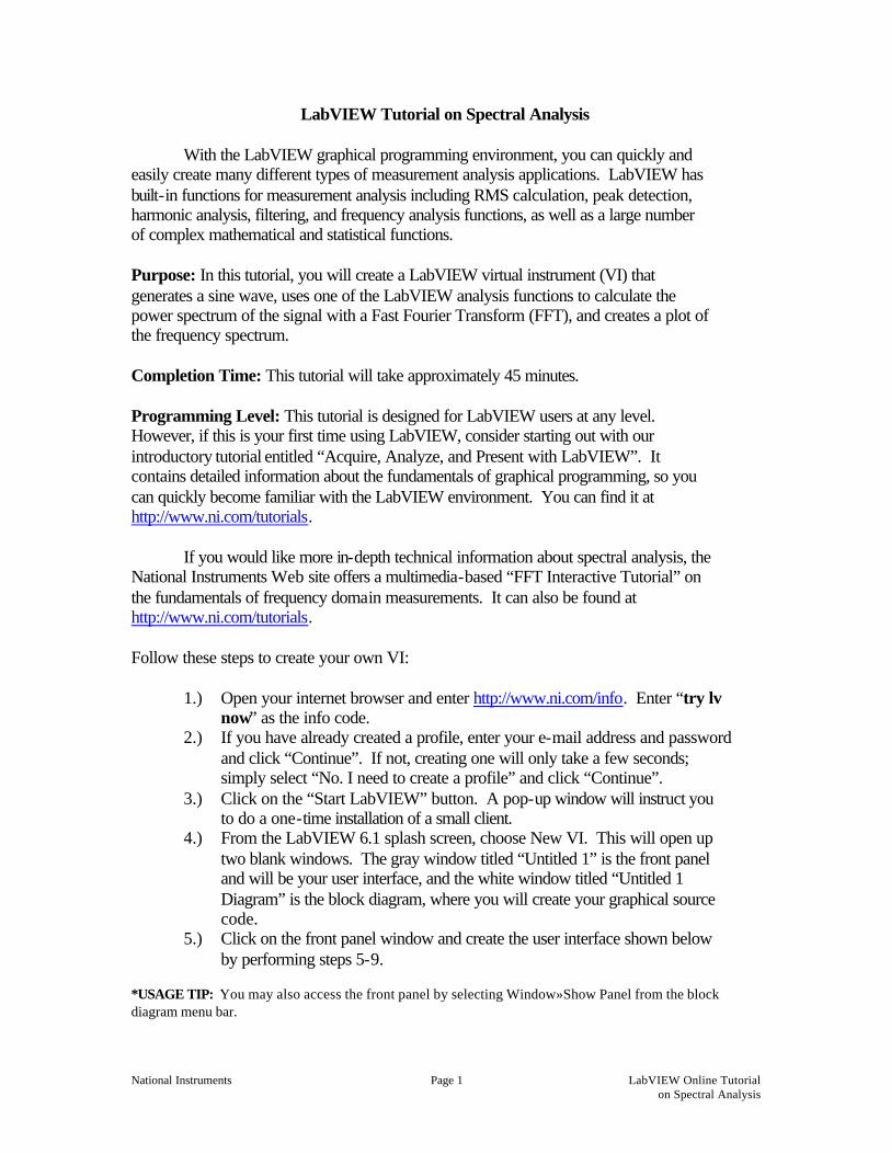
National Instruments Page 1 LabVIEW Online Tutorial on Spectral Analysis LabVIEW Tutorial on Spectral Analysis With the LabVIEW graphical programming environment, you can quickly and easily create many different types of measurement analysis applications. LabVIEW has built-in functions for measurement analysis including RMS calculation, peak detection, harmonic analysis, filtering, and frequency analysis functions, as well as a large number of complex mathematical and statistical functions. Purpose: In this tutorial, you will create a LabVIEW virtual instrument (VI) that generates a sine wave, uses one of the LabVIEW analysis functions to calculate the power spectrum of the signal with a Fast Fourier Transform (FFT), and creates a plot of the frequency spectrum. Completion Time: This tutorial will take approximately 45 minutes. Programming Level: This tutorial is designed for LabVIEW users at any level. However, if this is your first time using LabVIEW, consider starting out with our introductory tutorial entitled “Acquire, Analyze, and Present with LabVIEW”. It contains detailed information about the fundamentals of graphical programming, so you can quickly become familiar with the LabVIEW environment. You can find it at http://www.ni.com/tutorials . If you would like more in-depth technical information about spectral analysis, the National Instruments Web site offers a multimedia-based “FFT Interactive Tutorial” on the fundamentals of frequency domain measurements. It can also be found at http://www.ni.com/tutorials . Follow these steps to create your own VI: 1.) Open your internet browser and enter http://www.ni.com/info . Enter “try lv now ” as the info code. 2.) If you have already created a profile, enter your e-mail address and password and click “Continue”. If not, creating one will only take a few seconds; simply select “No. I need to create a profile” and click “Continue”. 3.) Click on the “Start LabVIEW” button. A pop-up window will instruct you to do a one-time installation of a small client. 4.) From the LabVIEW 6.1 splash screen, choose New VI. This will open up two blank windows. The gray window titled “Untitled 1” is the front panel and will be your user interface, and the white window titled “Untitled 1 Diagram” is the block diagram, where you will create your graphical source code. 5.) Click on the front panel window and create the user interface shown below by performing steps 5-9. *USAGE TIP: You may also access the front panel by selecting Window»Show Panel from the block diagram menu bar.
Transcript of LabVIEW Tutorial on Spectral Analysis - National...
National Instruments Page 1 LabVIEW Online Tutorial on Spectral Analysis
LabVIEW Tutorial on Spectral Analysis With the LabVIEW graphical programming environment, you can quickly and easily create many different types of measurement analysis applications. LabVIEW has built-in functions for measurement analysis including RMS calculation, peak detection, harmonic analysis, filtering, and frequency analysis functions, as well as a large number of complex mathematical and statistical functions. Purpose: In this tutorial, you will create a LabVIEW virtual instrument (VI) that generates a sine wave, uses one of the LabVIEW analysis functions to calculate the power spectrum of the signal with a Fast Fourier Transform (FFT), and creates a plot of the frequency spectrum. Completion Time: This tutorial will take approximately 45 minutes. Programming Level: This tutorial is designed for LabVIEW users at any level. However, if this is your first time using LabVIEW, consider starting out with our introductory tutorial entitled “Acquire, Analyze, and Present with LabVIEW”. It contains detailed information about the fundamentals of graphical programming, so you can quickly become familiar with the LabVIEW environment. You can find it at http://www.ni.com/tutorials.
If you would like more in-depth technical information about spectral analysis, the National Instruments Web site offers a multimedia-based “FFT Interactive Tutorial” on the fundamentals of frequency domain measurements. It can also be found at http://www.ni.com/tutorials.
Follow these steps to create your own VI:
1.) Open your internet browser and enter http://www.ni.com/info. Enter “try lv now” as the info code.
2.) If you have already created a profile, enter your e-mail address and password and click “Continue”. If not, creating one will only take a few seconds; simply select “No. I need to create a profile” and click “Continue”.
3.) Click on the “Start LabVIEW” button. A pop-up window will instruct you to do a one-time installation of a small client.
4.) From the LabVIEW 6.1 splash screen, choose New VI. This will open up two blank windows. The gray window titled “Untitled 1” is the front panel and will be your user interface, and the white window titled “Untitled 1 Diagram” is the block diagram, where you will create your graphical source code.
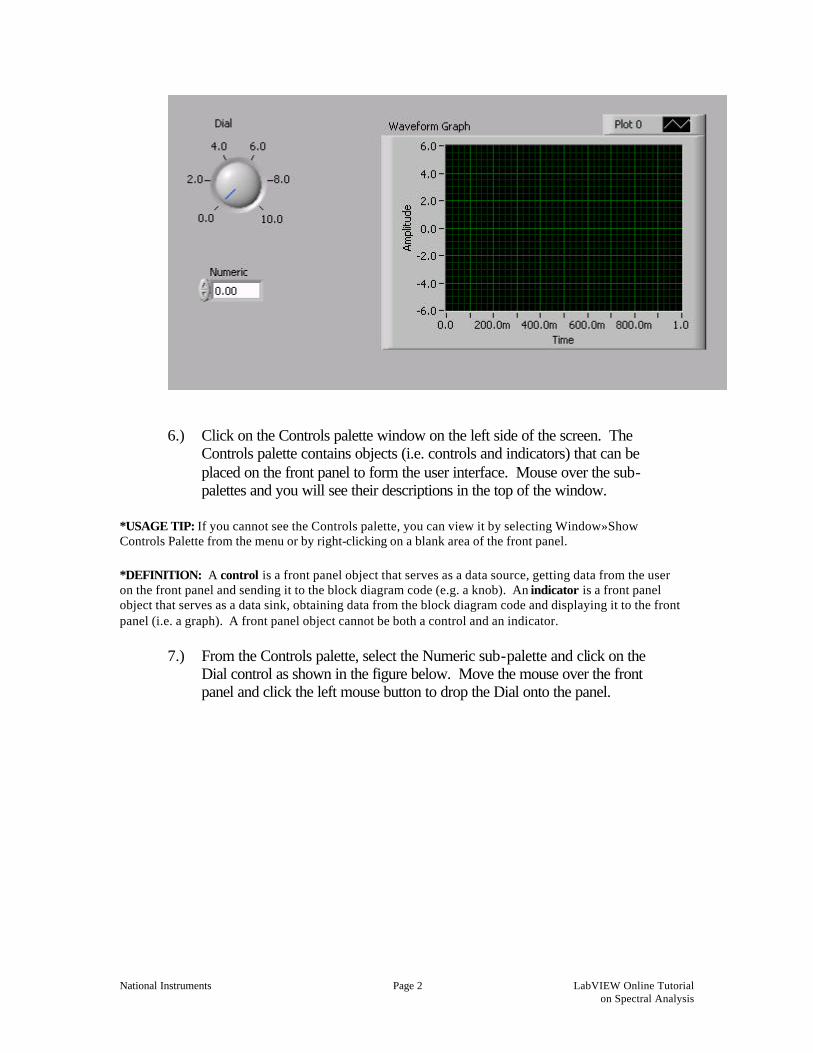
5.) Click on the front panel window and create the user interface shown below by performing steps 5-9.
*USAGE TIP: You may also access the front panel by selecting Window»Show Panel from the block diagram menu bar.
National Instruments Page 2 LabVIEW Online Tutorial on Spectral Analysis
6.) Click on the Controls palette window on the left side of the screen. The
Controls palette contains objects (i.e. controls and indicators) that can be placed on the front panel to form the user interface. Mouse over the sub-palettes and you will see their descriptions in the top of the window.
*USAGE TIP: If you cannot see the Controls palette, you can view it by selecting Window»Show Controls Palette from the menu or by right-clicking on a blank area of the front panel.
*DEFINITION: A control is a front panel object that serves as a data source, getting data from the user on the front panel and sending it to the block diagram code (e.g. a knob). An indicator is a front panel object that serves as a data sink, obtaining data from the block diagram code and displaying it to the front panel (i.e. a graph). A front panel object cannot be both a control and an indicator.
7.) From the Controls palette, select the Numeric sub-palette and click on the
Dial control as shown in the figure below. Move the mouse over the front panel and click the left mouse button to drop the Dial onto the panel.

National Instruments Page 3 LabVIEW Online Tutorial on Spectral Analysis
*USAGE TIP: You can reposition the Dial control on the panel by clicking and dragging with the positioning tool, shown as an arrow on the Tools palette. To select the positioning tool, either click on it in the Tools palette or press the <TAB> key to switch the currently selected tool until the positioning tool is shown. *USAGE TIP: If you cannot see the Tools palette, select Window»Show Tools Palette from the menu.
8.) From the Numeric sub-palette, choose the Digital Control, and drop it onto
the front panel. 9.) Click on the up arrow at the top of the Numeric sub-palette window to go
back to the Controls palette, as shown below.
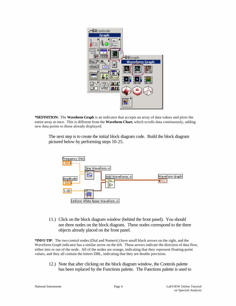
10.) From the Controls palette, select the Graph sub-palette and click on the
Waveform Graph as shown below. Place it onto the front panel.
National Instruments Page 4 LabVIEW Online Tutorial on Spectral Analysis
*DEFINITION: The Waveform Graph is an indicator that accepts an array of data values and plots the entire array at once. This is different from the Waveform Chart, which scrolls data continuously, adding new data points to those already displayed.
The next step is to create the initial block diagram code. Build the block diagram pictured below by performing steps 10-25.
11.) Click on the block diagram window (behind the front panel). You should see three nodes on the block diagram. These nodes correspond to the three objects already placed on the front panel.
*INFO TIP: The two control nodes (Dial and Numeric) have small black arrows on the right, and the Waveform Graph indicator has a similar arrow on the left. These arrows indicate the direction of data flow, either into or out of the node. All of the nodes are orange, indicating that they represent floating-point values, and they all contain the letters DBL, indicating that they are double precision.
12.) Note that after clicking on the block diagram window, the Controls palette has been replaced by the Functions palette. The Functions palette is used to
National Instruments Page 5 LabVIEW Online Tutorial on Spectral Analysis
build the block diagram. It contains all of the LabVIEW functions that can be combined to create your custom application.
13.) Reposition the Functions palette so that you can view the entire window on your screen.
*USAGE TIP: If you cannot see the Functions palette, you may show it manually by selecting Window»Show Functions Palette from the menu.
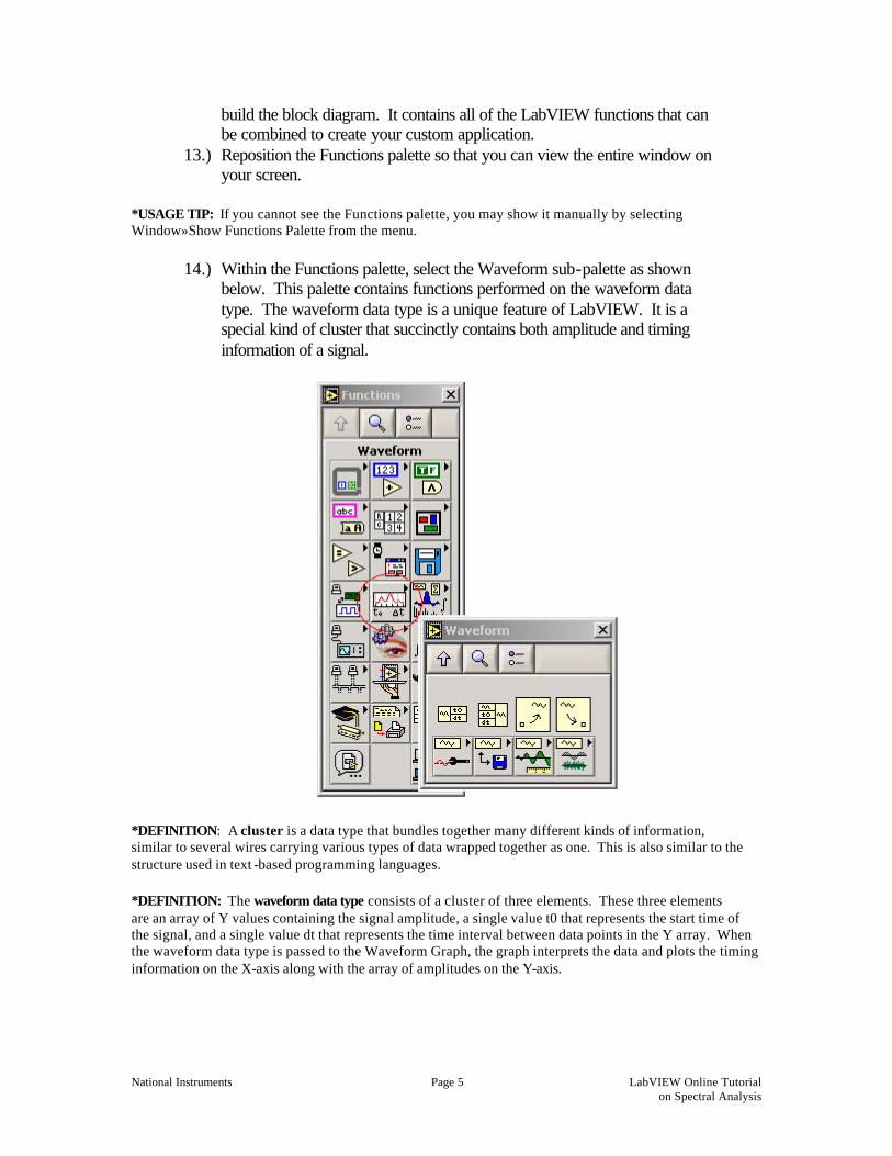
14.) Within the Functions palette, select the Waveform sub-palette as shown
below. This palette contains functions performed on the waveform data type. The waveform data type is a unique feature of LabVIEW. It is a special kind of cluster that succinctly contains both amplitude and timing information of a signal.
*DEFINITION: A cluster is a data type that bundles together many different kinds of information, similar to several wires carrying various types of data wrapped together as one. This is also similar to the structure used in text -based programming languages.
*DEFINITION: The waveform data type consists of a cluster of three elements. These three elements are an array of Y values containing the signal amplitude, a single value t0 that represents the start time of the signal, and a single value dt that represents the time interval between data points in the Y array. When the waveform data type is passed to the Waveform Graph, the graph interprets the data and plots the timing information on the X-axis along with the array of amplitudes on the Y-axis.
National Instruments Page 6 LabVIEW Online Tutorial on Spectral Analysis
14.) Within the Waveform palette, select the Waveform Generation menu. The functions in this menu automatically generate many commonly used waveforms.
15.) Choose the Sine Wave.vi and drop it onto the block diagram.
*USAGE TIP: If you would like more information on how the Sine Wave.vi or any other VI works, simply activate the Context Help by selecting Help»Show Context Help or by pressing <CTRL><H>. Put the mouse pointer on any object in the block diagram, and the context help window will give a description of that VI or object. For additional in-depth information about a VI click on the “Click here for more help” button inside the Context Help window to open the LabVIEW Help page for that item. The LabVIEW Help page contains specific information about each input and output and about the function of the VI. You can also view the front panel and/or block diagram of the SineWave.vi by double-clicking on the node or right-clicking on it and selecting Open Front Panel.
16.) From the same Waveform Generation menu, choose the Uniform White Noise Waveform.vi and place it on the block diagram.
17.) Using the wiring tool (shown as a spool of wire in the Tools palette), place the mouse over the Sine Wave.vi and notice that the input and output terminals appear on the edges of the VI icon. The input or output terminal that the wiring tool is currently pointing to blinks on the block diagram as well as in the Context Help window (press <CTRL><H>), and its label is displayed in a tip-strip.
18.) Select the ‘frequency’ input by clicking on the upper left input terminal. A broken wire will now trail the mouse as you move it.
19.) Click on the Dial control and notice that a solid orange wire has been connected from the Dial control node to the Sine Wave.vi ‘frequency’ input. The orange color of the wire symbolizes a floating-point value.
*USAGE TIP: You can click the left mouse button anytime during wiring to lock the current position of the wire onto the screen. Then you can move the mouse up or down to better control how the wire is placed. You can also move wires around by clicking and dragging them with the positioning tool (arrow). To cancel the placement of a wire, click the right mouse button during wiring or highlight the undesired wire and press <DELETE>. To eliminate all broken wires on the block diagram at once, press <CTRL><B>. The VI will not run if there are broken wires.
20.) Rename the Dial control by double-clicking on the label with the labeling
tool (capital “A”). This will highlight the label, allowing you to type in new text. Change the label to “Frequency (Hz)”, since this dial has been wired to control the frequency input to the Sine Wave.vi.
21.) Using the same method explained in steps 16-18 above, wire the ‘amplitude’ input of the Sine Wave.vi to the Numeric digital control node and change the label of the Numeric control to “Amplitude.”
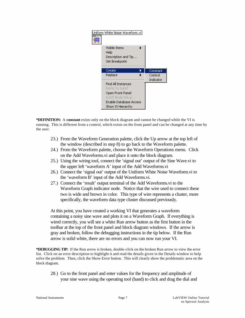
22.) With the wiring tool, right-click on the ‘amplitude’ input of the Uniform White Noise Waveform.vi and select Create»Constant as shown below. The default amplitude of the noise is 1.00. You can change this value by double-clicking on it with the labeling tool (capital “A”) and typing in a new number.
National Instruments Page 7 LabVIEW Online Tutorial on Spectral Analysis
*DEFINITION: A constant exists only on the block diagram and cannot be changed while the VI is running. This is different from a control, which exists on the front panel and can be changed at any time by the user.
23.) From the Waveform Generation palette, click the Up arrow at the top left of the window (described in step 8) to go back to the Waveform palette.
24.) From the Waveform palette, choose the Waveform Operations menu. Click on the Add Waveforms.vi and place it onto the block diagram.
25.) Using the wiring tool, connect the ‘signal out’ output of the Sine Wave.vi to the upper left ‘waveform A’ input of the Add Waveforms.vi
26.) Connect the ‘signal out’ output of the Uniform White Noise Waveform.vi to the ‘waveform B’ input of the Add Waveforms.vi.
27.) Connect the ‘result’ output terminal of the Add Waveforms.vi to the Waveform Graph indicator node. Notice that the wire used to connect these two is wide and brown in color. This type of wire represents a cluster, more specifically, the waveform data type cluster discussed previously.
At this point, you have created a working VI that generates a waveform containing a noisy sine wave and plots it on a Waveform Graph. If everything is wired correctly, you will see a white Run arrow button as the first button in the toolbar at the top of the front panel and block diagram windows. If the arrow is gray and broken, follow the debugging instructions in the tip below. If the Run arrow is solid white, there are no errors and you can now run your VI.
*DEBUGGING TIP: If the Run arrow is broken, double-click on the broken Run arrow to view the error list. Click on an error description to highlight it and read the details given in the Details window to help solve the problem. Then, click the Show Error button. This will clearly show the problematic area on the block diagram.
28.) Go to the front panel and enter values for the frequency and amplitude of
your sine wave using the operating tool (hand) to click and drag the dial and
National Instruments Page 8 LabVIEW Online Tutorial on Spectral Analysis
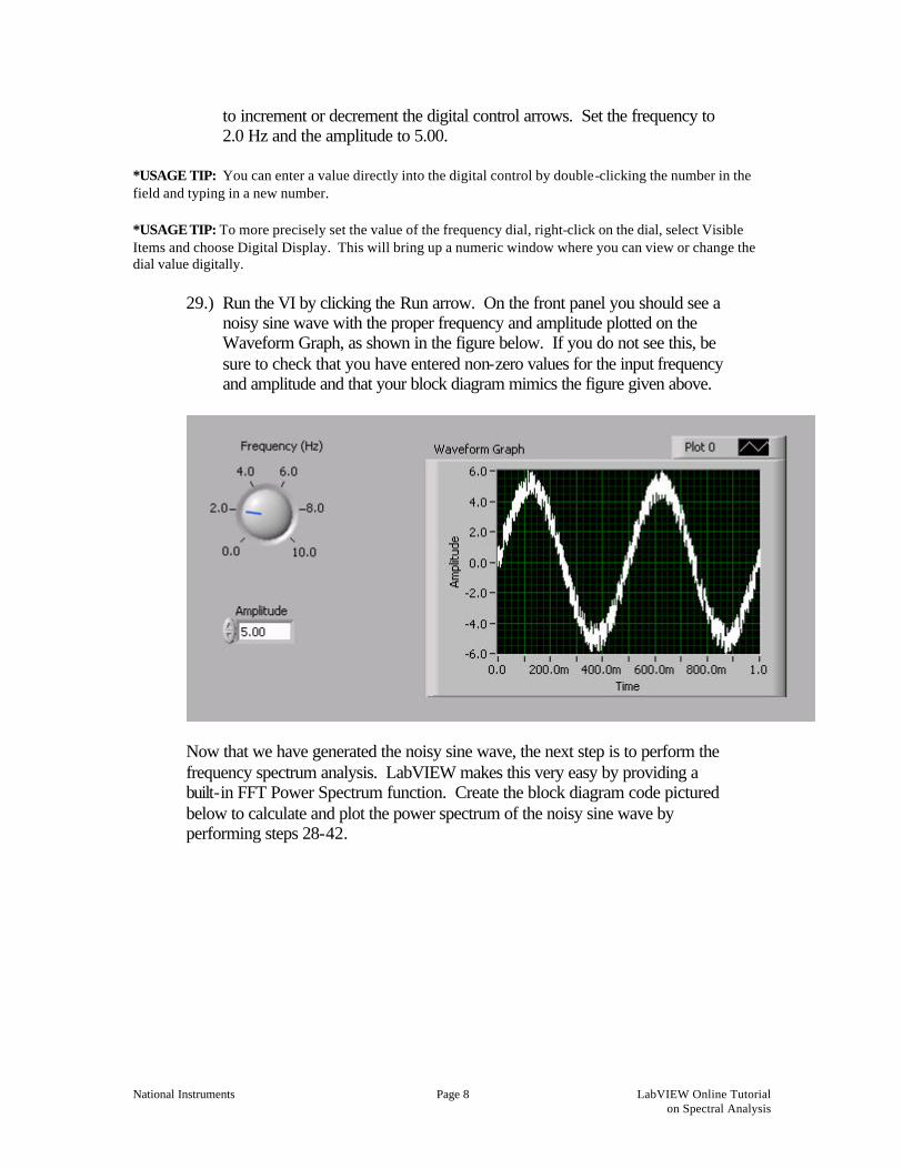
to increment or decrement the digital control arrows. Set the frequency to 2.0 Hz and the amplitude to 5.00.
*USAGE TIP: You can enter a value directly into the digital control by double-clicking the number in the field and typing in a new number.
*USAGE TIP: To more precisely set the value of the frequency dial, right-click on the dial, select Visible Items and choose Digital Display. This will bring up a numeric window where you can view or change the dial value digitally.
29.) Run the VI by clicking the Run arrow. On the front panel you should see a
noisy sine wave with the proper frequency and amplitude plotted on the Waveform Graph, as shown in the figure below. If you do not see this, be sure to check that you have entered non-zero values for the input frequency and amplitude and that your block diagram mimics the figure given above.
Now that we have generated the noisy sine wave, the next step is to perform the frequency spectrum analysis. LabVIEW makes this very easy by providing a built-in FFT Power Spectrum function. Create the block diagram code pictured below to calculate and plot the power spectrum of the noisy sine wave by performing steps 28-42.
National Instruments Page 9 LabVIEW Online Tutorial on Spectral Analysis
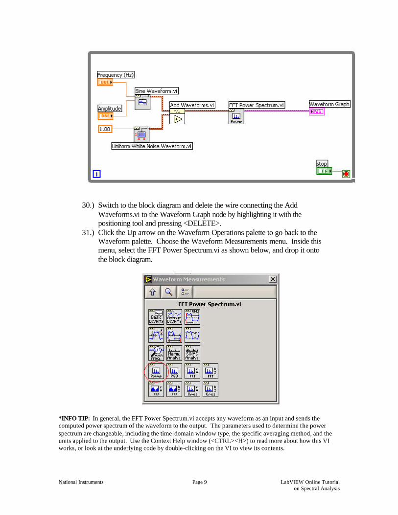
30.) Switch to the block diagram and delete the wire connecting the Add
Waveforms.vi to the Waveform Graph node by highlighting it with the positioning tool and pressing <DELETE>.
31.) Click the Up arrow on the Waveform Operations palette to go back to the Waveform palette. Choose the Waveform Measurements menu. Inside this menu, select the FFT Power Spectrum.vi as shown below, and drop it onto the block diagram.
*INFO TIP: In general, the FFT Power Spectrum.vi accepts any waveform as an input and sends the computed power spectrum of the waveform to the output. The parameters used to determine the power spectrum are changeable, including the time-domain window type, the specific averaging method, and the units applied to the output. Use the Context Help window (<CTRL><H>) to read more about how this VI works, or look at the underlying code by double-clicking on the VI to view its contents.
National Instruments Page 10 LabVIEW Online Tutorial on Spectral Analysis
32.) Place the wiring tool on the FFT Power Spectrum.vi icon to view the input and output terminals.
33.) Connect the ‘time signal’ input of the FFT Power Spectrum.vi to the ‘result’ output of the Add Waveforms.vi.
34.) Connect the ‘power spectrum’ output of the FFT Power Spectrum.vi to the Waveform Graph indicator node. Notice that the wire connecting the FFT Power Spectrum.vi to the Waveform Graph is pink. The pink color in this case denotes a general cluster data type.
*DEFINITION: The Waveform Graph node itself has also changed from brown to pink. This graph is polymorphic, meaning that it accepts many different types of data, including waveforms, clusters, and arrays. The ability to use polymorphic functions is a feature of LabVIEW that provides versatility in your programming by not restricting you to traditional explicit type casting rules.
Next, we will add a While Loop to run continuous iterations of the sine wave generation and frequency analysis. This is necessary in order to utilize the averaging features of the FFT Power Spectrum.vi.
35.) From the Waveform Measurements palette, click the Up arrow twice to go
back to the general Functions palette. 36.) Select the Structures sub-palette and choose the While Loop structure. Then,
place the While Loop around the existing code by clicking and holding down the mouse button at the upper left corner of the block diagram window and dragging the box to enclose the entire diagram.
37.) Go to the front panel. Click the Up arrow until you see the general Controls palette.
38.) Select the Boolean sub-palette, and choose the STOP button. Drop the STOP button onto the front panel.
*USAGE TIP: It is important to always have a way to stop any loops that you create in LabVIEW. The STOP button is the best way to easily control while loops.
39.) Go back to the block diagram and locate the STOP button node. Use the positioning tool to drag this node into the while loop, if it is not already there.
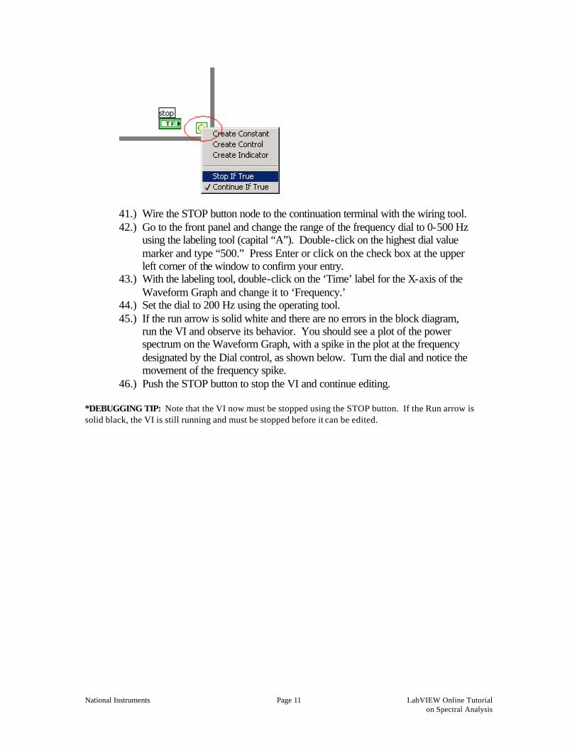
40.) Right-click on the continuation terminal (green circular arrow) of the while loop in the bottom right corner and select Stop if True, as shown below. You will see the terminal change from a green arrow to a red stop sign.
National Instruments Page 11 LabVIEW Online Tutorial on Spectral Analysis
41.) Wire the STOP button node to the continuation terminal with the wiring tool. 42.) Go to the front panel and change the range of the frequency dial to 0-500 Hz
using the labeling tool (capital “A”). Double-click on the highest dial value marker and type “500.” Press Enter or click on the check box at the upper left corner of the window to confirm your entry.
43.) With the labeling tool, double-click on the ‘Time’ label for the X-axis of the Waveform Graph and change it to ‘Frequency.’
44.) Set the dial to 200 Hz using the operating tool. 45.) If the run arrow is solid white and there are no errors in the block diagram,
run the VI and observe its behavior. You should see a plot of the power spectrum on the Waveform Graph, with a spike in the plot at the frequency designated by the Dial control, as shown below. Turn the dial and notice the movement of the frequency spike.
46.) Push the STOP button to stop the VI and continue editing.
*DEBUGGING TIP: Note that the VI now must be stopped using the STOP button. If the Run arrow is solid black, the VI is still running and must be stopped before it can be edited.
National Instruments Page 12 LabVIEW Online Tutorial on Spectral Analysis
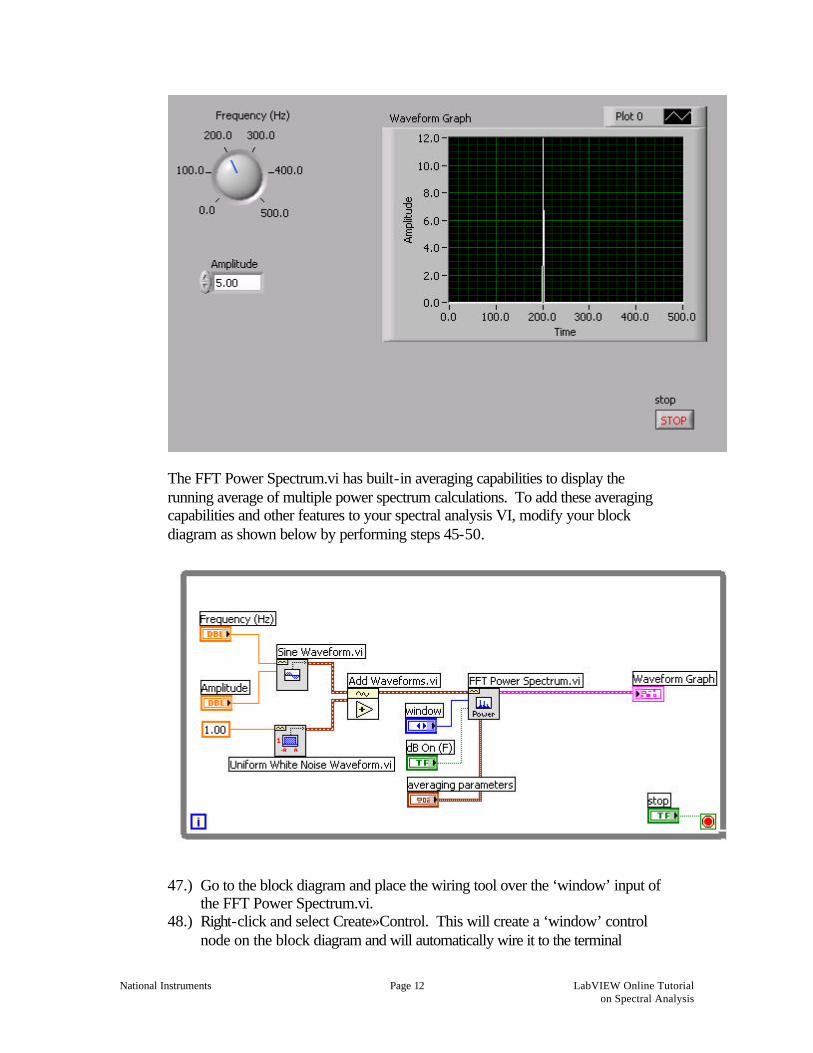
The FFT Power Spectrum.vi has built-in averaging capabilities to display the running average of multiple power spectrum calculations. To add these averaging capabilities and other features to your spectral analysis VI, modify your block diagram as shown below by performing steps 45-50.
47.) Go to the block diagram and place the wiring tool over the ‘window’ input of
the FFT Power Spectrum.vi. 48.) Right-click and select Create»Control. This will create a ‘window’ control
node on the block diagram and will automatically wire it to the terminal
National Instruments Page 13 LabVIEW Online Tutorial on Spectral Analysis
from which it was created. It will also place a new control on the front panel.
49.) Use the positioning tool to click on the ‘window’ node and move it away from the other input terminals. Be sure when you are moving objects to highlight the entire object, not just the label.
50.) Locate the new ring control on the front panel (it may be off the screen below). Use the positioning tool to click on the ‘window’ control and drag it to a better location near the other front panel objects.
51.) Repeat the above steps to create controls for the ‘averaging parameters’ input, and the ‘dB On’ input. Doing this will add to the front panel a cluster control with elements specifying the ‘averaging parameters’, as well as a vertical slide switch control for ‘dB On’.
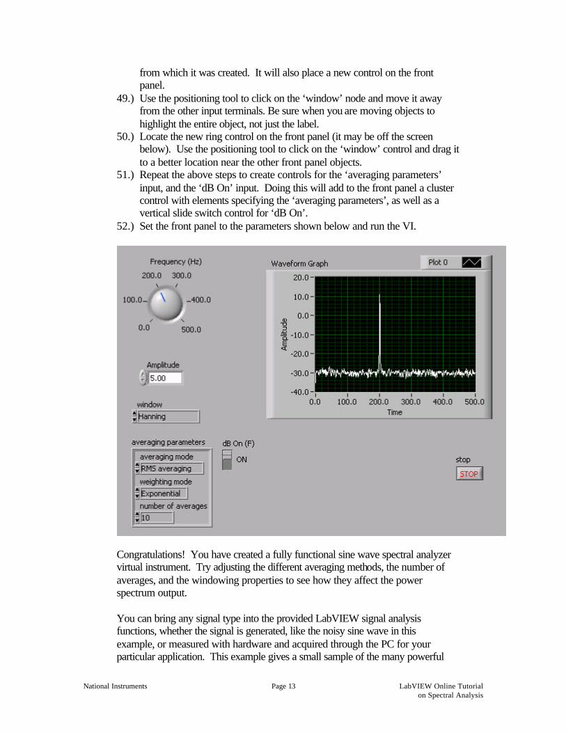
52.) Set the front panel to the parameters shown below and run the VI.
Congratulations! You have created a fully functional sine wave spectral analyzer virtual instrument. Try adjusting the different averaging methods, the number of averages, and the windowing properties to see how they affect the power spectrum output. You can bring any signal type into the provided LabVIEW signal analysis functions, whether the signal is generated, like the noisy sine wave in this example, or measured with hardware and acquired through the PC for your particular application. This example gives a small sample of the many powerful
National Instruments Page 14 LabVIEW Online Tutorial on Spectral Analysis
tools that LabVIEW has to offer and demonstrates the ease with which you can create your own custom signal analysis applications.