Laboratory scale experiments and preliminary modelling to investigate basin scale tidal stream

energy extraction Scott Draper#1, Tim Stallard*2, Peter Stansby*3, Stephen Way+4 and Thomas Adcockǂ5

#Centre for Offshore Foundation Systems, The University of Western Australia 35 Stirling Highway, Crawley, 6009, Australia.

1scott.draper@uwa.edu.au *School of Mechanical, Aerospace and Civil Engineering, The University of Manchester

Manchester, M13 9PL, UK. 2tim.stallard@manchester.ac.uk

3peter.k.stansby@manchester.ac.uk #GL Garrad Hassan

+St Vincent’s Works, Silverthorne Lane, Bristol, BS2 0QD, UK. 4Stephen.Way@gl-garradhassan.com

ǂDepartment of Engineering Science, University of Oxford Parks Road, Oxford, OX1 3PJ, UK.

5thomas.adcock@eng.ox.ac.uk

Abstract— This paper summarizes a set of model scale experiments that were undertaken to investigate the momentum deficit imparted by strips of porous discs emulating model scale tidal stream turbine fences. This was undertaken as part of the Energy Technologies Institute PerAWAT project. In the experiments the strips were placed in (1) a uniform model scale tidal channel and (2) a model scale tidal channel containing a headland with sloping sides. Both steady and oscillatory flow experiments were performed. Experimental results are discussed in terms of the effect of the emulators on the flow field, and the measured drag force on the emulators.

For the tidal channel experiments the emulator had a notable ‘blockage’ effect, leading to a depth-averaged velocity deficit behind the emulator and a faster depth-averaged bypass velocity around the emulator. Furthermore, the force on the emulator increased as it occupied a greater fraction of the channels width. For the headland experiments, when the emulator was placed near to the tip of the headland, point velocity measurements indicated an acceleration of flow in the gap between the fence and the headland tip. Surprisingly, however, there was little change in force on the emulator as its position relative to the tip of the headland was varied.

Comparisons are made between the experimental results and depth-averaged numerical simulations. Assuming a fixed resistivity coefficient and blockage ratio for the porous discs within the emulator, the numerical simulations reproduce the emulator force measurements reasonably well across the full range of experiments, but tend to underestimate the velocity deficit behind the emulator.

Keywords— Tidal stream energy, shallow water flow, resource characterisation, depth-averaged modelling.

I. INTRODUCTION Previous modelling of tidal stream energy extraction at the

scale of a coastal site has been almost exclusively confined to theoretical models (i.e. Garrett and Cummins (2005) and Vennell (2010)) or depth-averaged numerical modelling (i.e. Sutherland et al. (2007), Karsten et al. (2008), Draper et al. (2013) and Adcock et al. (2013)), in which energy extraction is modelled as a simple added bed roughness or momentum sink. Validation of such models (numerical or theoretical) has therefore been limited to cross comparison with different numerical or theoretical models and fails to assess directly if the physics captured by the models is adequate for useful quantification of the change in shallow water flows due to energy extraction.

In this paper we present results from a series of large scale laboratory experiments in which tidal devices are emulated by strips of porous discs and are placed in a uniform tidal channel and close to a coastal headland with sloping sides. The choice to model a tidal channel and a coastal headland was made because numerous sites around the UK where tidal streams are significant resemble these coastal features (i.e. Pentland Firth (channel), Anglesey (headland), Mull of Kintyre (headland), etc.). The experiments were specifically designed to provide detailed information on the changes to natural tidal currents due to the presence of tidal devices, and the momentum deficit of the tidal devices (in terms of drag force).

We also present a preliminary comparison of experimental measurements of the flow field and momentum deficit with predictions from a depth-averaged numerical model. Tidal devices in the numerical model are represented as a line

Fig. 1 Experimental setup. (Top) plan view, axes are in m. (Bottom) Section A-A, not to scale.

sink of momentum using the approach outlined in Draper et al. (2010).

The remainder of the paper is structured as follows. First we outline the experimental setup and present the experimental results. Next we introduced the depth-averaged model and calibrate it for the momentum sink of the emulators and natural friction in the channel. We then compare depth-average modelling results with the experimental results, and finally provide discussion and conclusions.

II. EXPERIMENTAL SETUP A 20 m long by 9 m wide channel was constructed in the

wave and current basin at HR Wallingford, UK (see Fig. 1 and Fig. 2). The walls of the channel were constructed with breeze blocks and the bed of the channel comprised gravel stones (to a depth of approximately 15 mm) with median grain diameter of 8.43 mm and coefficient of uniformity ~1.5.

Tests were conducted in the channel alone and with the addition of a headland, which measured 2.5 m at the channel wall and extended 1.5 m out into the channel (see Fig. 1). The headland was skirted by a linearly sloping bathymetry extending over a width of 1.5 m. This bathymetry was at a depth of 0.1 m below still water level adjacent to the headland, and sloped at a gradient of 1V:15H.

In each of the experiments the still water depth was set to approximately 0.2 m (see Table 1 for actual measured values) and both oscillatory and steady flows conditions were simulated. For the tidal channel experiments the depth-averaged steady flow velocity was ~0.54 m/s, and the oscillatory flow had period 1200 seconds and amplitude of ~ 0.54 m/s. For experiments in the channel with the headland the depth-averaged steady flow velocity (at the inlet to the channel) was ~0.33 m/s, and the oscillatory flow had period 1200 seconds and reached a peak velocity of ~ 0.33 m/s.

A. Scaling of tidal flow The channel and headland were built as large as possible in

the experiments to minimize scaling effects. Based on channel length, the model tidal channel represents a 1:100-350 scale model of an actual tidal channel in the UK, whilst based on breadth of the headland, the headland model represents a 1:200-2000 scale representation of an actual UK headland.

To ensure the experimental flow conditions were a reasonable reproduction of that at actual coastal sites, the geometry, seabed roughness and flow velocities discussed above were chosen to best achieve similitude in Froude number, tidal excursion and stability number. Similarity of

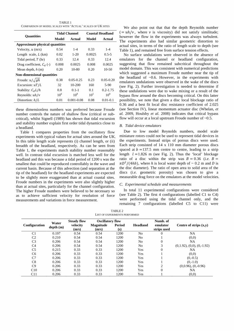
TABLE 1 COMPARISON OF MODEL SCALES WITH ‘ACTUAL’ SCALES OF UK SITES

Quantities Tidal Channel Coastal Headland

Model Actual Model Actual Approximate physical quantities Velocity, 𝑢 (m/s) 0.54 1-4 0.33 1-4 Length scale, 𝐿 (km) 0.02 1-20 0.0025 0.5-5 Tidal period, 𝑇 (hr) 0.33 12.4 0.33 12.4 Drag coefficient, 𝐶𝑑 (-) 0.008 0.0025 0.008 0.0025 Mean depth, h (m) 0.20 10-80 0.20 10-50

Non-dimensional quantities Froude: 𝑢/�𝑔ℎ 0.38 0.05-0.25 0.23 0.05-0.20 Excursion: 𝑢𝑇/𝐿 32 10-200 160 5-90 Stability: 𝐶𝑑𝐿/ℎ 0.8 0.1-1 0.1 0.2-1.75 Reynolds: 𝑢ℎ/𝜈 106 108 105 108 Distortion: ℎ/𝐿 0.01 0.001-0.08 0.08 0.01-0.1

these dimensionless numbers was preferred because Froude number controls the nature of shallow flow (critical or sub-critical), whilst Signell (1989) has shown that tidal excursion and stability number explain first order tidal dynamics close to a headland.

Table 1 compares properties from the oscillatory flow experiments with typical values for actual sites around the UK. In this table length scale represents (i) channel length, or (ii) breadth of the headland, respectively. As can be seen from Table 1, the experiments match stability number reasonably well. In contrast tidal excursion is matched less well for the headland and this was because a tidal period of 1200 s was the smallest that could be reproduced controllably in the wave and current basin. Because of this advection (and separation at the tip of the headland) for the headland experiments are expected to be slightly more exaggerated than at actual coastal sites. Froude numbers in the experiments were also slightly higher than at actual sites, particularly for the channel configuration. The higher Froude numbers were believed to be necessary so as to achieve sufficient velocity for resolution of force measurements and variations in force measurement.

We also point out that that the depth Reynolds number

( = 𝑢ℎ/𝜈 , where 𝜈 is viscosity) did not satisfy similitude; however the flow in the experiments was always turbulent. The experiments also had similar geometric distortion to actual sites, in terms of the ratio of length scale to depth (see Table 1), and remained free from surface tension effects.

No surface undulations were observed in the absence of emulators for the channel or headland configuration, suggesting that flow remained subcritical throughout the model domain. This was consistent with numerical predictions which suggested a maximum Froude number near the tip of the headland of ~0.6. However, in the experiments with emulators undulations were observed in the wake of the discs (see Fig. 2). Further investigation is needed to determine if these undulations were due to wake mixing or a result of the bypass flow around the discs becoming critical. On this latter possibility, we note that given a disc local blockage ratio of 0.36 and a best fit local disc resistance coefficient of 2.025 (see Section IV), linear momentum actuator disc (Whelan, et al. 2009, Houlsby et al. 2008) indicates that critical bypass flow will occur at a local upstream Froude number of ~0.5.

B. Tidal device emulators Due to low model Reynolds numbers, model scale

miniature rotors could not be used to represent tidal devices in the experiments. Instead strips of porous discs were used. Each strip consisted of 14 x 110 mm diameter porous discs spaced at 𝑏 =137.5 mm centre to centre, leading to a strip length 𝑙 =1.826 m (see Fig. 2). Thus the ‘local’ blockage ratio of a disc within the strip was 𝐵 = 0.36 (i.e. 𝐵 =𝜋𝐷2/(4ℎ𝑏), where ℎ is local water depth of ~ 0.2 m and 𝐷 is the disc diameter). The ratio of open area to solid area of the discs (i.e. geometric porosity) was chosen to give a measurable drag force on the emulators at the model velocities.

C. Experimental schedule and measurements In total 11 experimental configurations were considered

(see Table 2). The first 4 configurations (labelled C1 to C4) were performed using the tidal channel only, and the remaining 7 configurations (labelled C5 to C11) were

TABLE 2 LIST OF EXPERIMENTS PERFORMED

Configuration Water depth (m)

Steady flow velocity

(m/s)

Oscillatory flow Headland

Numb. of emulator

strips used Centre of strips (x,y) Magnitude

(m/s) Period

(s) C1 0.197 0.54 0.54 1200 No 0 NA C2 0.210 0.54 0.54 1200 No 1 (0,0) C3 0.206 0.54 0.54 1200 No 0 NA C4 0.206 0.54 0.54 1200 No 3 (0,1.92), (0,0), (0,-1.92) C5 0.215 0.33 0.33 1200 Yes 0 NA C6 0.206 0.33 0.33 1200 Yes 1 (0,0) C7 0.206 0.33 0.33 1200 Yes 1 (0,-0.5) C8 0.206 0.33 0.33 1200 Yes 1 (0,-1.0) C9 0.206 0.33 0.33 1200 Yes 2 (0,0.96), (0,-0.96) C10 0.206 0.33 0.33 1200 Yes 0 NA C11 0.206 0.33 0.33 1200 Yes 1 (0,0)

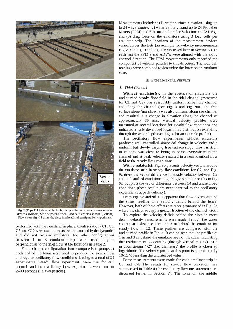
Fig. 2 (Top) Tidal channel, including support beams to mount measurement devices. (Middle) Strip of porous discs. Load cells are also shown. (Bottom) Flow (from right) behind the discs in a headland configuration experiment.

performed with the headland in place. Configurations C1, C3, C5 and C10 were used to measure undisturbed hydrodynamics and did not require emulators. For other configurations between 1 to 3 emulator strips were used, aligned perpendicular to the inlet flow at the locations in Table 2.

For each test configuration four computerised pumps at each end of the basin were used to produce the steady flow and regular oscillatory flow conditions, leading to a total of 22 experiments. Steady flow experiments were run for 400 seconds and the oscillatory flow experiments were run for 2400 seconds (i.e. two periods).

Measurements included: (1) water surface elevation using up to 24 wave gauges; (2) water velocity using up to 24 Propeller Meters (PPM) and 6 Acoustic Doppler Velocimeters (ADVs); and (3) drag force on the emulators using 3 load cells per emulator strip. The locations of the measurement devices varied across the tests (an example for velocity measurements is given in Fig. 9 and Fig. 10; discussed later in Section V). In each test the PPM’s and ADV’s were aligned with the along channel direction. The PPM measurements only recorded the component of velocity parallel to this direction. The load cell readings were combined to determine the force on an emulator strip.

III. EXPERIMENTAL RESULTS

A. Tidal Channel Without emulator(s): In the absence of emulators the

undisturbed steady flow field in the tidal channel (measured for C1 and C3) was reasonably uniform across the channel and along the channel (see Fig. 3 and Fig. 9a). The free surface slope (not shown) was also uniform along the channel and resulted in a change in elevation along the channel of approximately 30 mm. Vertical velocity profiles were measured at several locations for steady flow conditions and indicated a fully developed logarithmic distribution extending through the water depth (see Fig. 4 for an example profile).

The oscillatory flow experiments without emulators produced well controlled sinusoidal change in velocity and a uniform but slowly varying free surface slope. The variation in velocity was close to being in phase everywhere in the channel and at peak velocity resulted in a near identical flow field to the steady flow conditions.

With emulator(s): Fig. 9b presents velocity vectors around the emulator strip in steady flow conditions for C2, and Fig. 9c gives the vector difference in steady velocity between C2 and undisturbed conditions. Fig. 9d gives similar results to Fig. 9c, but plots the vector difference between C4 and undisturbed conditions (these results are near identical to the oscillatory experiments at peak velocity).

From Fig. 9c and 9d it is apparent that flow diverts around the strips, leading to a velocity deficit behind the fence. However, both of these effects are more pronounced in Fig. 9d, where the strips occupy a greater fraction of the channel width.

To explore the velocity deficit behind the discs in more detail, velocity measurements were made through the water column at a distance 1 m and 3 m behind the emulator for steady flow in C2. These profiles are compared with the undisturbed profile in Fig. 4. It can be seen that the profiles at 1 m and 3 m behind the emulator are not the same, indicating that readjustment is occurring (through vertical mixing). At 3 m downstream (~27 disc diameters) the profile is closer to logarithmic. The velocity profile at this point is approximately 10-15 % less than the undisturbed value.

Force measurements were made for each emulator strip in C2 and C4. The results for steady flow conditions are summarised in Table 4 (the oscillatory flow measurements are discussed further in Section V). The force on the middle

Row of discs

Fig. 3 Variation in velocity across the channel.

Fig. 4 Thick solid line is a logarithmic fit to velocity measurements for

configuration C1 without an emulator (crosses). Remaining points are for configuration C2 with emulator at location (1,0) (circles) and (3,0) (triangles).

Vertical axes are height above seabed in meters.

emulator in C4 is smaller than the end emulators, indicating that the force is not uniform along the fence; although the variation is small. The emulator force is measurably greater in C4, where the strips occupy a greater fraction of the channel cross-section, than in C2. This is indicative of a ‘blockage effect’ at the scale of the strip; i.e. the blockage 𝑙/𝑊, where 𝑊 is channel width.

B. Coastal Headland Without emulator(s): Velocity measurements obtained for

configurations C5 and C10 in steady flow are shown in Fig. 10a. Unfortunately, some of the measurement devices did not return measurements; however the data that has been obtained suggests that upstream of the headland the flow was relatively uniform across the width of the channel. The upstream inlet velocity at 𝑥 = −10 m is approximately 0.3 m/s (at 100 mm above flume bed). In contrast, close to the headland there is a

clear acceleration as the flow passes around the tip of the headland, and an associated reduction in velocity downstream of the headland (for 𝑦 < ~ −2.5 m) in the wake behind the headland.

Close to the tip of the headland velocity measurements through the water depth were measured for steady flow conditions. These measurements were obtained for three locations: (-1,-1), (2,-2) and (-1,-2), and are given in Fig. 5. At points (-1,-1) and (-1,-2), which are located upstream of the headland, the velocity measurements are reasonably consistent with a logarithmic distribution. In contrast, downstream of the headland at point (2,-2) the flow is no longer logarithmic. This is consistent with secondary flows close to the tip of the headland.

Unfortunately no data was recovered for oscillatory flow without emulators, however from observations during the experiments the peak velocity in the oscillatory experiments was very similar to the steady flow results.

With emulator(s): Fig. 10b presents velocity vectors around the emulator strip and headland for configuration C6 in steady flow. To better explore the difference between these measurements and the flow measurements without emulators, Fig. 10c gives the vector difference in steady velocity between C6 and undisturbed conditions. Although the measurement points are sparse the results tend to indicate an acceleration of flow in the gap between the fence and the headland tip. This is most pronounced in Fig. 10d, which presents the vector difference in steady velocity between C9 and undisturbed conditions (i.e. C5).

Very similar results to those shown in Fig. 10 were obtained at peak flow conditions in the positive 𝑥-direction for the oscillatory flow experiments. At peak conditions on the reverse flow (i.e. negative 𝑥 -direction) the velocities were generally smaller in magnitude, but this was due to an unintentional asymmetry in the inlet flow rate over the tidal cycle.

Fig. 5 Velocity near to headland tip in configuration C5 without an emulator. A logarithmic distribution is fitted to measurements at (-1,-2)

(circles). Velocities are also given at (-1,-1) (triangles) and (2,-2) (crosses). Vertical axes are height above seabed in meters.

0

0.2

0.4

0.6

0.8

1

-4.5 -3.5 -2.5 -1.5 -0.5 0.5 1.5 2.5 3.5 4.5

Vel

ocity

in x

-dire

ctio

n [m

/s]

y [m]

x = 3 mx = 1 mx = -1 mx = -3 m

0

0.02

0.04

0.06

0.08

0.1

0.12

0.14

0.16

0 0.5Velocity, u [m/s]

0.01

0.1

0 0.5Velocity, u [m/s]

0

0.02

0.04

0.06

0.08

0.1

0.12

0.14

0.16

0 0.5Velocity, u [m/s]

0.01

0.1

0 0.5Velocity, u [m/s]

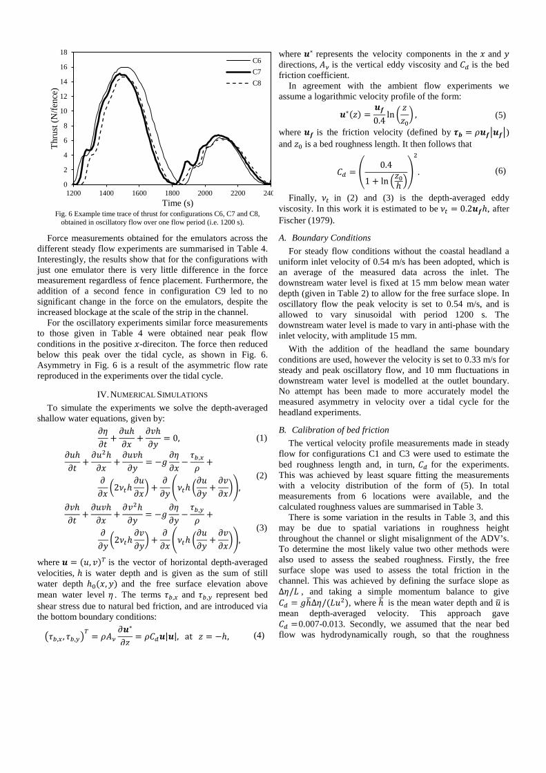
Fig. 6 Example time trace of thrust for configurations C6, C7 and C8,

obtained in oscillatory flow over one flow period (i.e. 1200 s).

Force measurements obtained for the emulators across the different steady flow experiments are summarised in Table 4. Interestingly, the results show that for the configurations with just one emulator there is very little difference in the force measurement regardless of fence placement. Furthermore, the addition of a second fence in configuration C9 led to no significant change in the force on the emulators, despite the increased blockage at the scale of the strip in the channel.

For the oscillatory experiments similar force measurements to those given in Table 4 were obtained near peak flow conditions in the positive 𝑥-direciton. The force then reduced below this peak over the tidal cycle, as shown in Fig. 6. Asymmetry in Fig. 6 is a result of the asymmetric flow rate reproduced in the experiments over the tidal cycle.

IV. NUMERICAL SIMULATIONS To simulate the experiments we solve the depth-averaged

shallow water equations, given by: 𝜕𝜂𝜕𝑡

+𝜕𝑢ℎ𝜕𝑥

+𝜕𝑣ℎ𝜕𝑦

= 0, (1)

𝜕𝑢ℎ𝜕𝑡

+𝜕𝑢2ℎ𝜕𝑥

+𝜕𝑢𝑣ℎ𝜕𝑦

= −𝑔𝜕𝜂𝜕𝑥

−𝜏𝑏,𝑥

𝜌+

𝜕𝜕𝑥

�2𝜈𝑡ℎ𝜕𝑢𝜕𝑥� +

𝜕𝜕𝑦

�𝜈𝑡ℎ �𝜕𝑢𝜕𝑦

+𝜕𝑣𝜕𝑥��,

(2)

𝜕𝑣ℎ𝜕𝑡

+𝜕𝑢𝑣ℎ𝜕𝑥

+𝜕𝑣2ℎ𝜕𝑦

= −𝑔𝜕𝜂𝜕𝑦

−𝜏𝑏,𝑦

𝜌+

𝜕𝜕𝑦

�2𝜈𝑡ℎ𝜕𝑣𝜕𝑦� +

𝜕𝜕𝑥

�𝜈𝑡ℎ �𝜕𝑢𝜕𝑦

+𝜕𝑣𝜕𝑥��,

(3)

where 𝒖 = (𝑢, 𝑣)𝑇 is the vector of horizontal depth-averaged velocities, ℎ is water depth and is given as the sum of still water depth ℎ0(𝑥,𝑦) and the free surface elevation above mean water level 𝜂 . The terms 𝜏𝑏,𝑥 and 𝜏𝑏,𝑦 represent bed shear stress due to natural bed friction, and are introduced via the bottom boundary conditions:

�𝜏𝑏,𝑥 , 𝜏𝑏,𝑦�𝑇 = 𝜌𝐴𝜈

𝜕𝒖∗

𝜕𝑧= 𝜌𝐶𝑑𝒖|𝒖|, at 𝑧 = −ℎ, (4)

where 𝒖∗ represents the velocity components in the 𝑥 and 𝑦 directions, 𝐴𝜈 is the vertical eddy viscosity and 𝐶𝑑 is the bed friction coefficient.

In agreement with the ambient flow experiments we assume a logarithmic velocity profile of the form:

𝒖∗(𝑧) =𝒖𝒇0.4

ln �𝑧𝑧0� , (5)

where 𝒖𝒇 is the friction velocity (defined by 𝝉𝒃 = 𝜌𝒖𝒇�𝒖𝒇�) and 𝑧0 is a bed roughness length. It then follows that

𝐶𝑑 = �0.4

1 + ln �𝑧0ℎ ��

2

. (6)

Finally, 𝜈𝑡 in (2) and (3) is the depth-averaged eddy viscosity. In this work it is estimated to be 𝜈𝑡 = 0.2𝒖𝒇ℎ, after Fischer (1979).

A. Boundary Conditions For steady flow conditions without the coastal headland a

uniform inlet velocity of 0.54 m/s has been adopted, which is an average of the measured data across the inlet. The downstream water level is fixed at 15 mm below mean water depth (given in Table 2) to allow for the free surface slope. In oscillatory flow the peak velocity is set to 0.54 m/s, and is allowed to vary sinusoidal with period 1200 s. The downstream water level is made to vary in anti-phase with the inlet velocity, with amplitude 15 mm.

With the addition of the headland the same boundary conditions are used, however the velocity is set to 0.33 m/s for steady and peak oscillatory flow, and 10 mm fluctuations in downstream water level is modelled at the outlet boundary. No attempt has been made to more accurately model the measured asymmetry in velocity over a tidal cycle for the headland experiments.

B. Calibration of bed friction The vertical velocity profile measurements made in steady

flow for configurations C1 and C3 were used to estimate the bed roughness length and, in turn, 𝐶𝑑 for the experiments. This was achieved by least square fitting the measurements with a velocity distribution of the form of (5). In total measurements from 6 locations were available, and the calculated roughness values are summarised in Table 3.

There is some variation in the results in Table 3, and this may be due to spatial variations in roughness height throughout the channel or slight misalignment of the ADV’s. To determine the most likely value two other methods were also used to assess the seabed roughness. Firstly, the free surface slope was used to assess the total friction in the channel. This was achieved by defining the surface slope as Δ𝜂/𝐿 , and taking a simple momentum balance to give 𝐶𝑑 = 𝑔ℎ�Δ𝜂/(𝐿𝑢2), where ℎ� is the mean water depth and 𝑢� is mean depth-averaged velocity. This approach gave 𝐶𝑑 =0.007-0.013. Secondly, we assumed that the near bed flow was hydrodynamically rough, so that the roughness

0

2

4

6

8

10

12

14

16

18

1200 1400 1600 1800 2000 2200 240

Thru

st (N

/fenc

e)

Time (s)

C6C7C8

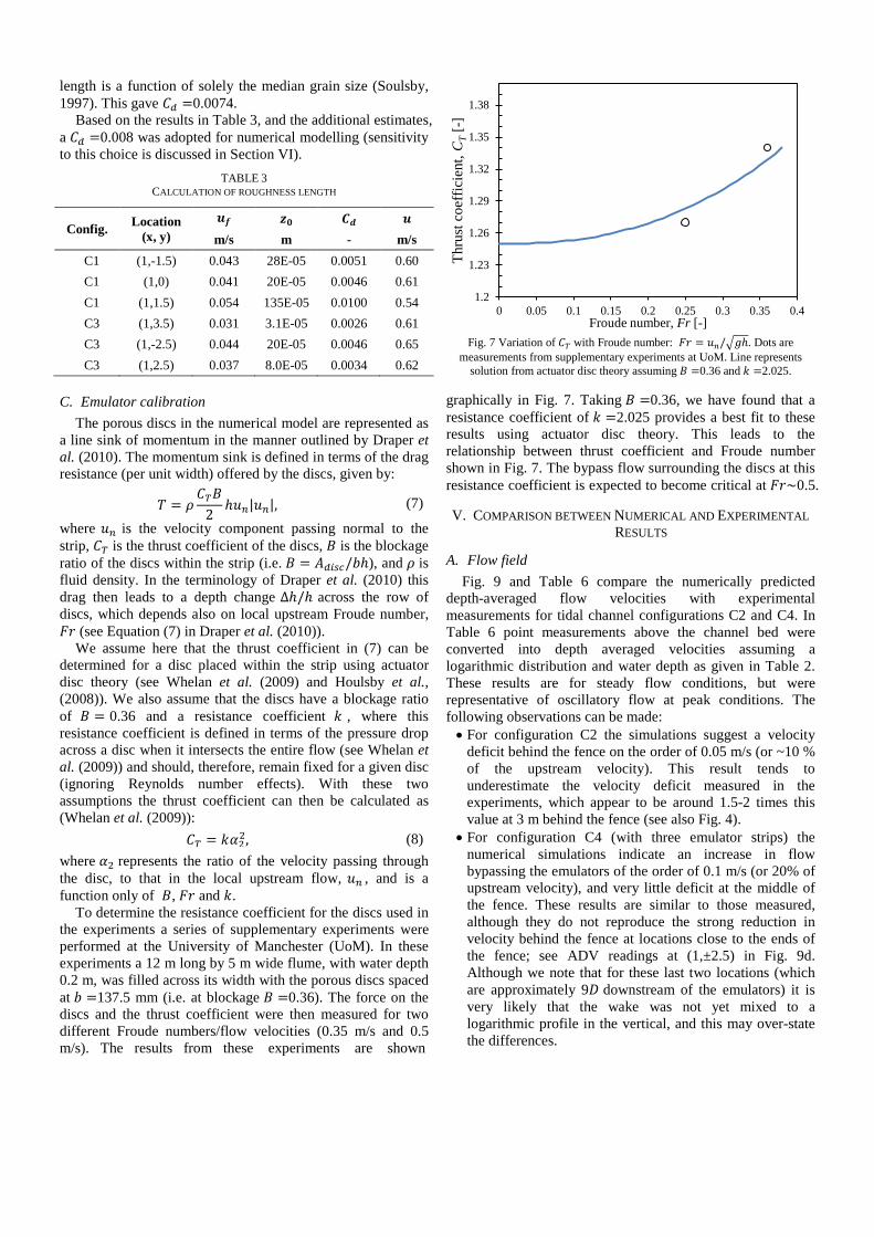
length is a function of solely the median grain size (Soulsby, 1997). This gave 𝐶𝑑 =0.0074.

Based on the results in Table 3, and the additional estimates, a 𝐶𝑑 =0.008 was adopted for numerical modelling (sensitivity to this choice is discussed in Section VI).

TABLE 3 CALCULATION OF ROUGHNESS LENGTH

Config. Location (x, y)

𝒖𝒇 𝒛𝟎 𝑪𝒅 𝒖 m/s m - m/s

C1 (1,-1.5) 0.043 28E-05 0.0051 0.60 C1 (1,0) 0.041 20E-05 0.0046 0.61 C1 (1,1.5) 0.054 135E-05 0.0100 0.54 C3 (1,3.5) 0.031 3.1E-05 0.0026 0.61 C3 (1,-2.5) 0.044 20E-05 0.0046 0.65 C3 (1,2.5) 0.037 8.0E-05 0.0034 0.62

C. Emulator calibration

The porous discs in the numerical model are represented as a line sink of momentum in the manner outlined by Draper et al. (2010). The momentum sink is defined in terms of the drag resistance (per unit width) offered by the discs, given by:

𝑇 = 𝜌𝐶𝑇𝐵

2ℎ𝑢𝑛|𝑢𝑛|, (7)

where 𝑢𝑛 is the velocity component passing normal to the strip, 𝐶𝑇 is the thrust coefficient of the discs, 𝐵 is the blockage ratio of the discs within the strip (i.e. 𝐵 = 𝐴𝑑𝑖𝑠𝑐/𝑏ℎ), and 𝜌 is fluid density. In the terminology of Draper et al. (2010) this drag then leads to a depth change Δℎ/ℎ across the row of discs, which depends also on local upstream Froude number, 𝐹𝑟 (see Equation (7) in Draper et al. (2010)).

We assume here that the thrust coefficient in (7) can be determined for a disc placed within the strip using actuator disc theory (see Whelan et al. (2009) and Houlsby et al., (2008)). We also assume that the discs have a blockage ratio of 𝐵 = 0.36 and a resistance coefficient 𝑘 , where this resistance coefficient is defined in terms of the pressure drop across a disc when it intersects the entire flow (see Whelan et al. (2009)) and should, therefore, remain fixed for a given disc (ignoring Reynolds number effects). With these two assumptions the thrust coefficient can then be calculated as (Whelan et al. (2009)):

𝐶𝑇 = 𝑘𝛼22, (8) where 𝛼2 represents the ratio of the velocity passing through the disc, to that in the local upstream flow, 𝑢𝑛 , and is a function only of 𝐵, 𝐹𝑟 and 𝑘.

To determine the resistance coefficient for the discs used in the experiments a series of supplementary experiments were performed at the University of Manchester (UoM). In these experiments a 12 m long by 5 m wide flume, with water depth 0.2 m, was filled across its width with the porous discs spaced at 𝑏 =137.5 mm (i.e. at blockage 𝐵 =0.36). The force on the discs and the thrust coefficient were then measured for two different Froude numbers/flow velocities (0.35 m/s and 0.5 m/s). The results from these experiments are shown

Fig. 7 Variation of 𝐶𝑇 with Froude number: 𝐹𝑟 = 𝑢𝑛/�𝑔ℎ. Dots are

measurements from supplementary experiments at UoM. Line represents solution from actuator disc theory assuming 𝐵 =0.36 and 𝑘 =2.025.

graphically in Fig. 7. Taking 𝐵 =0.36, we have found that a resistance coefficient of 𝑘 =2.025 provides a best fit to these results using actuator disc theory. This leads to the relationship between thrust coefficient and Froude number shown in Fig. 7. The bypass flow surrounding the discs at this resistance coefficient is expected to become critical at 𝐹𝑟~0.5.

V. COMPARISON BETWEEN NUMERICAL AND EXPERIMENTAL RESULTS

A. Flow field Fig. 9 and Table 6 compare the numerically predicted

depth-averaged flow velocities with experimental measurements for tidal channel configurations C2 and C4. In Table 6 point measurements above the channel bed were converted into depth averaged velocities assuming a logarithmic distribution and water depth as given in Table 2. These results are for steady flow conditions, but were representative of oscillatory flow at peak conditions. The following observations can be made: • For configuration C2 the simulations suggest a velocity

deficit behind the fence on the order of 0.05 m/s (or ~10 % of the upstream velocity). This result tends to underestimate the velocity deficit measured in the experiments, which appear to be around 1.5-2 times this value at 3 m behind the fence (see also Fig. 4).

• For configuration C4 (with three emulator strips) the numerical simulations indicate an increase in flow bypassing the emulators of the order of 0.1 m/s (or 20% of upstream velocity), and very little deficit at the middle of the fence. These results are similar to those measured, although they do not reproduce the strong reduction in velocity behind the fence at locations close to the ends of the fence; see ADV readings at (1,±2.5) in Fig. 9d. Although we note that for these last two locations (which are approximately 9𝐷 downstream of the emulators) it is very likely that the wake was not yet mixed to a logarithmic profile in the vertical, and this may over-state the differences.

1.2

1.23

1.26

1.29

1.32

1.35

1.38

0 0.05 0.1 0.15 0.2 0.25 0.3 0.35 0.4

Thru

st c

oeffi

cien

t, C

T [-]

Froude number, Fr [-]

A similar comparison between the depth-averaged predicted flow velocities and experimental measurements are given in Fig. 10 and Table 7 for configurations C6 and C9. In Table 7 point measurements above the channel bed were converted into depth averaged velocities assuming a logarithmic distribution and water depth as given in Table 2. Again these results are for steady flow conditions only, but were representative of oscillatory flow at peak flow conditions. The following observations can be made: • The numerical model is in good agreement on the

‘upstream side’ of the headland, but shows much less agreement near to the boundary of the recirculation zone (i.e. 𝑦~ −2.5 m) immediately downstream of the headland.

• The numerical model tends to suggest an increase in velocity in the gap between the emulator and the tip of the headland, which depends on the location of the emulator(s). This increase varies from ~0.05 m/s (for C6) to ~0.2 m/s (for C9). This is somewhat consistent with the experiments, although it should also be noted that the measurement points were sparse for the headland configuration experiments and the velocity vector differences (for example Fig. 10a and Fig. 10b) may have larger relative error than other results due to, for example, slight movement of the ADV between experiments.

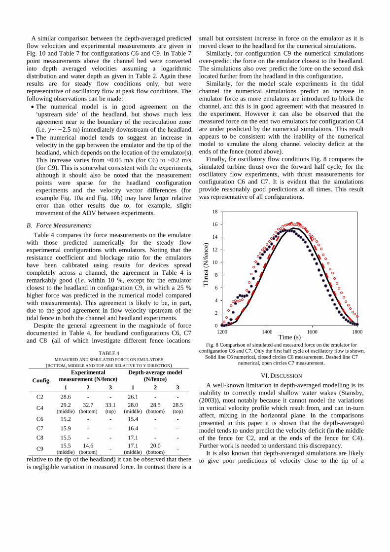
B. Force Measurements Table 4 compares the force measurements on the emulator

with those predicted numerically for the steady flow experimental configurations with emulators. Noting that the resistance coefficient and blockage ratio for the emulators have been calibrated using results for devices spread completely across a channel, the agreement in Table 4 is remarkably good (i.e. within 10 %, except for the emulator closest to the headland in configuration C9, in which a 25 % higher force was predicted in the numerical model compared with measurements). This agreement is likely to be, in part, due to the good agreement in flow velocity upstream of the tidal fence in both the channel and headland experiments.

Despite the general agreement in the magnitude of force documented in Table 4, for headland configurations C6, C7 and C8 (all of which investigate different fence locations

TABLE 4

MEASURED AND SIMULATED FORCE ON EMULATORS (BOTTOM, MIDDLE AND TOP ARE RELATIVE TO Y DIRECTION)

Config. Experimental

measurement (N/fence) Depth-average model

(N/fence) 1 2 3 1 2 3

C2 28.6 - - 26.1 - -

C4 29.2 (middle)

32.7 (bottom)

33.1 (top)

28.0 (middle)

28.5 (bottom)

28.5 (top)

C6 15.2 - - 15.4 - - C7 15.9 - - 16.4 - - C8 15.5 - - 17.1 - -

C9 15.5 (middle)

14.6 (bottom) - 17.1

(middle) 20.0

(bottom) -

relative to the tip of the headland) it can be observed that there is negligible variation in measured force. In contrast there is a

small but consistent increase in force on the emulator as it is moved closer to the headland for the numerical simulations.

Similarly, for configuration C9 the numerical simulations over-predict the force on the emulator closest to the headland. The simulations also over predict the force on the second disk located further from the headland in this configuration.

Similarly, for the model scale experiments in the tidal channel the numerical simulations predict an increase in emulator force as more emulators are introduced to block the channel, and this is in good agreement with that measured in the experiment. However it can also be observed that the measured force on the end two emulators for configuration C4 are under predicted by the numerical simulations. This result appears to be consistent with the inability of the numerical model to simulate the along channel velocity deficit at the ends of the fence (noted above).

Finally, for oscillatory flow conditions Fig. 8 compares the simulated turbine thrust over the forward half cycle, for the oscillatory flow experiments, with thrust measurements for configuration C6 and C7. It is evident that the simulations provide reasonably good predictions at all times. This result was representative of all configurations.

Fig. 8 Comparison of simulated and measured force on the emulator for

configuration C6 and C7. Only the first half cycle of oscillatory flow is shown. Solid line C6 numerical, closed circles C6 measurement. Dashed line C7

numerical, open circles C7 measurement.

VI. DISCUSSION A well-known limitation in depth-averaged modelling is its

inability to correctly model shallow water wakes (Stansby, (2003)), most notably because it cannot model the variations in vertical velocity profile which result from, and can in-turn affect, mixing in the horizontal plane. In the comparisons presented in this paper it is shown that the depth-averaged model tends to under predict the velocity deficit (in the middle of the fence for C2, and at the ends of the fence for C4). Further work is needed to understand this discrepancy.

It is also known that depth-averaged simulations are likely to give poor predictions of velocity close to the tip of a

0

2

4

6

8

10

12

14

16

18

1200 1400 1600 1800

Thru

st (N

/fenc

e)

Time (s)

headland if secondary flows are significant (Signell, (1989)). Measurements made in steady flow (see Fig. 5) indicate that secondary flows are present in the experiments close to the headland, and these may explain in part why the numerical model over-predicted the measured emulator force as the fence was placed closer to the tip of the headland (i.e. the model may over-predict stream wise velocity near to the headland). However, further work is needed to determine if this was indeed the case.

Despite the discrepancies between the numerical model and the measurements for flow velocity, the present results show that the depth-averaged model can give reasonable estimates of force on a tidal fence. However we caution that the tidal devices in this paper were not placed in the wake of another fence, and the simulated velocities upstream of the emulator were in good agreement with the measurements.

Lastly we note that the numerical results discussed in Section V were obtained with best-estimate input parameters for bed friction, upstream velocity and water depth. Analysis has been conducted to investigate the sensitivity of the results to changes in these inputs. Table 5 summarises this analysis in terms of the simulated force on the emulator for C6 in steady flow. Collectively, the results in Table 5 indicate that small variations in the inputs can lead to a sizeable difference in emulator force; the most sensitive input being velocity. Across the different input parameters bed friction is likely to be the most uncertain; Table 5 suggests that the simulated results could vary between 10-20% across a likely range of drag coefficient.

TABLE 5 SENSITIVITY ANALYSIS FOR C6

Case 𝑪𝒅 Inlet velocity at mid-depth

(m/s)

Depth (m)

Force on emulator

(N) Best estimate 0.008 0.35 0.2 15.4 Low 𝐶𝑑 0.0025 0.35 0.2 14.5 High 𝐶𝑑 0.012 0.35 0.2 17.8 Low velocity 0.008 0.3 0.2 11.5 High velocity 0.008 0.4 0.2 22.5 Small depth 0.008 0.35 0.175 17.3 Large depth 0.008 0.35 0.25 14.9

VII. CONCLUSIONS Resource characterization for tidal stream energy is almost

exclusively performed with depth-averaged numerical models, guided by theoretical models. In this paper a series of large scale laboratory experiments have provided a data set by which to compare with depth-averaged simulations. The experimental results clearly show the ‘blockage effect’ experience by a tidal fence when it is placed in a narrow uniform channel, and provide data on the diversion of flow around a tidal fence placed close to coastal headland.

Comparisons between preliminary depth-averaged numerical modeling and the experimental measurements have shown that the numerical model can provide reasonable predictions of force on tidal fence (and presumably the power they extract), at least when the fence is not placed in a disturbed flow (i.e. a flow in the wake of a coastal feature or another fence). The simulations were less successful in reproducing velocity deficits behind the fence and in the wake of the headland. Further work is required to reconcile these differences.

ACKNOWLEDGMENT This work forms part of the ETI PerAWaT project. The ETI

is a public-private partnership between global industries – BP, Caterpillar, EDF, E.ON, Rolls-Royce and Shell – and the UK Government tasked with accelerating affordable, clean, secure technologies needed to help meet the UK meet its 2050 climate change targets. It makes targeted investments in projects in offshore wind, marine, distributed energy, buildings, energy storage and distribution, carbon capture and storage, transport and bio energy.

The authors would like to thank Mat Thomson and James Sutherland for valuable discussion on the experiments. The first author would like to acknowledge the support of the Lloyds Register Foundation.

REFERENCES [1] C. Garrett and P. Cummins (2005), The power potential of tidal

currents in channels, Proceedings of the Royal society London A, 461, pp. 2563-2572.

[2] R. Vennell (2010), Tuning turbines in a tidal channel, Journal Fluid Mechanics, 663, pp. 253-267.

[3] G. Sutherland, M. Foreman, and C. Garrett, (2007), Tidal current energy assessment for Johnstone Stait, Vancouver Island, Proc. IMechE, Part A: J. Power and Energy, 221(2), pp. 147-157.

[4] R.H. Karsten, J. M. McMillan, M.J. Lickley, and R.D. Haynes, (2008), Assessment of tidal current energy in the Minas Passage, Bay of Fundy, IMechE (222), pp. 493-507.

[5] T. A. A. Adcock, S. Draper, G. T. Houlsby, A. G. L. Borthwick, and S. Serhadlioglu, (2013a) Tidal energy resource of the Pentland Firth, Proceedings of the Royal Society, Part A, 469:20130072.

[6] S. Draper, A.G.L. Borthwick, and G. T. Houlsby, (2013). Energy Potential of a Tidal Fence Deployed near a Coastal Headland. Phil. Trans. Royal Society A, Vol. 371: 20120176

[7] S. Draper, G. T. Houlsby, M. L. G. Oldfield, and A. G. L. Borthwick (2010). Modeling Tidal Energy Extraction in a Depth Averaged Domain. IET Joun. Renew. Powr. Gen., Vol. 4, pp.545-554.

[8] G. T. Houlsby, S. Draper, and M.L.G. Oldfield, (2008). Application of linear momentum actuator disc theory to open channel flow. Oxford University Engineering Library Report No. 2297/08.

[9] R. Soulsby (1997) Dynamics of marine sands, Thomas Telford. [10] R.P. Signell. (1989) Tidal Dynamics and Dispersion around Coastal

Headlands. PhD thesis, Massachusetts Institute of Technology, 1989. [11] P. K. Stansby (2003) A mixing-length model for shallow turbulent

wakes, Journal Fluid Mechanics, 495, pp. 369-384. [12] J.I. Whelan, J.M.R. Graham, and J. Perio. (2009) A Free-Surface and

Blockage Correction for Tidal Turbines. Journal Fluid Mechanics, 624, pp. 281-291.

[13] H. B. Fischer, (1979) Mixing in inland and coastal waters, Academic Pr, 1979.

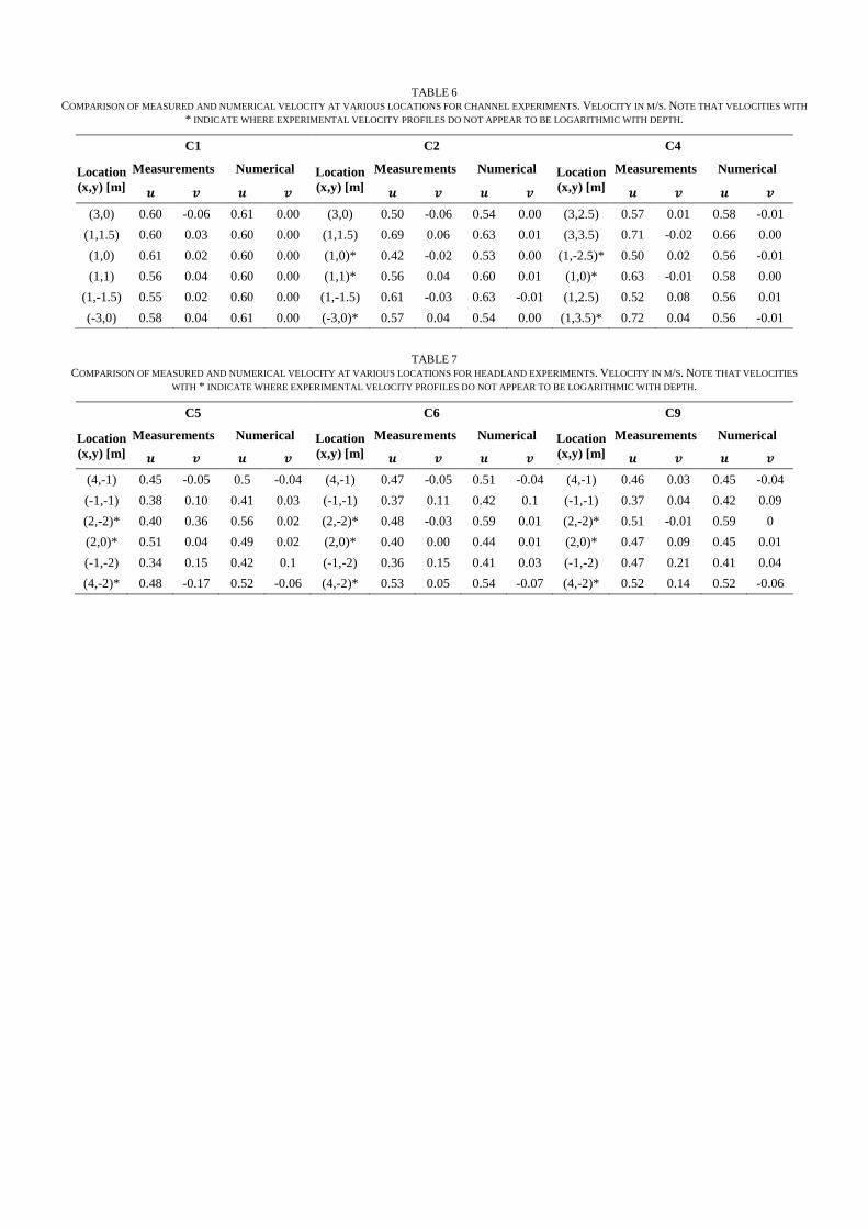
TABLE 6 COMPARISON OF MEASURED AND NUMERICAL VELOCITY AT VARIOUS LOCATIONS FOR CHANNEL EXPERIMENTS. VELOCITY IN M/S. NOTE THAT VELOCITIES WITH

* INDICATE WHERE EXPERIMENTAL VELOCITY PROFILES DO NOT APPEAR TO BE LOGARITHMIC WITH DEPTH.

C1 C2 C4

Location (x,y) [m]

Measurements Numerical Location (x,y) [m]

Measurements Numerical Location (x,y) [m]

Measurements Numerical

𝒖 𝒗 𝒖 𝒗 𝒖 𝒗 𝒖 𝒗 𝒖 𝒗 𝒖 𝒗 (3,0) 0.60 -0.06 0.61 0.00 (3,0) 0.50 -0.06 0.54 0.00 (3,2.5) 0.57 0.01 0.58 -0.01

(1,1.5) 0.60 0.03 0.60 0.00 (1,1.5) 0.69 0.06 0.63 0.01 (3,3.5) 0.71 -0.02 0.66 0.00 (1,0) 0.61 0.02 0.60 0.00 (1,0)* 0.42 -0.02 0.53 0.00 (1,-2.5)* 0.50 0.02 0.56 -0.01 (1,1) 0.56 0.04 0.60 0.00 (1,1)* 0.56 0.04 0.60 0.01 (1,0)* 0.63 -0.01 0.58 0.00

(1,-1.5) 0.55 0.02 0.60 0.00 (1,-1.5) 0.61 -0.03 0.63 -0.01 (1,2.5) 0.52 0.08 0.56 0.01 (-3,0) 0.58 0.04 0.61 0.00 (-3,0)* 0.57 0.04 0.54 0.00 (1,3.5)* 0.72 0.04 0.56 -0.01

TABLE 7 COMPARISON OF MEASURED AND NUMERICAL VELOCITY AT VARIOUS LOCATIONS FOR HEADLAND EXPERIMENTS. VELOCITY IN M/S. NOTE THAT VELOCITIES

WITH * INDICATE WHERE EXPERIMENTAL VELOCITY PROFILES DO NOT APPEAR TO BE LOGARITHMIC WITH DEPTH.

C5 C6 C9

Location (x,y) [m]

Measurements Numerical Location (x,y) [m]

Measurements Numerical Location (x,y) [m]

Measurements Numerical

𝒖 𝒗 𝒖 𝒗 𝒖 𝒗 𝒖 𝒗 𝒖 𝒗 𝒖 𝒗 (4,-1) 0.45 -0.05 0.5 -0.04 (4,-1) 0.47 -0.05 0.51 -0.04 (4,-1) 0.46 0.03 0.45 -0.04 (-1,-1) 0.38 0.10 0.41 0.03 (-1,-1) 0.37 0.11 0.42 0.1 (-1,-1) 0.37 0.04 0.42 0.09 (2,-2)* 0.40 0.36 0.56 0.02 (2,-2)* 0.48 -0.03 0.59 0.01 (2,-2)* 0.51 -0.01 0.59 0 (2,0)* 0.51 0.04 0.49 0.02 (2,0)* 0.40 0.00 0.44 0.01 (2,0)* 0.47 0.09 0.45 0.01 (-1,-2) 0.34 0.15 0.42 0.1 (-1,-2) 0.36 0.15 0.41 0.03 (-1,-2) 0.47 0.21 0.41 0.04 (4,-2)* 0.48 -0.17 0.52 -0.06 (4,-2)* 0.53 0.05 0.54 -0.07 (4,-2)* 0.52 0.14 0.52 -0.06

(a)

(b)

(c)

(d)

Fig. 9 (a) Velocity measurements at 50 mm ASB from C1 and C3. (b) Measurements (in red) and numerical velocities (in black) for C2. (c) Vector difference in velocity between C2 minus C1. Measurements at 50 mm ASB in

red, 70 mm ASB in green, 100 mm ASB in blue and 120 mm ASB in cyan. Numerical velocities in black. (d) Vector difference in velocity between C4 minus C3. Measurements at 50 mm above the flume bed in red. Numerical velocities in black. In all plots circles represent PPMs, and squares are ADVs, and blue line represents emulator. Scales: 0.5 m/s in figures (a) and (b); 0.1 m/s in figures (c) and (d).

-10 -8 -6 -4 -2 0 2 4 6 8 10

-4

-3

-2

-1

0

1

2

3

4

x [m]

y [m

]

-4 -2 0 2 4 6 8-2.5

-2

-1.5

-1

-0.5

0

0.5

1

1.5

2

2.5

x [m]

y [m

]

-4 -2 0 2 4 6 8-2.5

-2

-1.5

-1

-0.5

0

0.5

1

1.5

2

2.5

x [m]

y [m

]

-4 -2 0 2 4 6 8

-4

-3

-2

-1

0

1

2

3

4

x [m]

y [m

]

(a)

(b)

(c)

(d)

Fig. 10 (a) Velocity measurements at 120 mm ASB from C5 and C10. (b) Measurements (in red) and numerical velocities (in black) for C6. (Bottom left) Vector difference in velocity between C6 minus C5. Measurements at 120 mm ASB in red. Numerical velocities in black. (d) Vector difference in velocity between C9 minus C5. Measurements at 120 mm above the flume bed in red. Numerical velocities in black. In all plots circles represent

PPMs, and squares are ADVs. Blue line represents emulator. Scales: 0.3 m/s in top left and right figures. 0.1 m/s in bottom left and right figures.

-10 -8 -6 -4 -2 0 2 4 6 8 10

-4

-3

-2

-1

0

1

2

3

4

x [m]

y [m

]

-6 -4 -2 0 2 4 6 8

-4

-3

-2

-1

0

1

2

x [m]

y [m

]-6 -4 -2 0 2 4 6 8

-4

-3

-2

-1

0

1

2

x [m]

y [m

]

-6 -4 -2 0 2 4 6 8

-4

-3

-2

-1

0

1

2

x [m]y

[m]