Labor Markets and Poverty in Village Economies¤

Oriana Bandiera, Robin Burgess, Narayan Das,

Selim Gulesci, Imran Rasul, Munshi Sulaimany

March 2016

Abstract

We study how women’s choices over labor activities in village economies correlate with

poverty and whether enabling the poorest women to take on the activities of their richer

counterparts can set them on a sustainable trajectory out of poverty. To do this we conduct

a large-scale randomized control trial, covering over 21,000 households in 1,309 villages sur-

veyed four times over a seven year period, to evaluate a nationwide program in Bangladesh

that transfers livestock assets and skills to the poorest women. At baseline, the poorest

women mostly engage in low return and seasonal casual wage labor while wealthier women

solely engage in livestock rearing. The program enables poor women to start engaging in

livestock rearing, increasing their aggregate labor supply and earnings. This leads to asset

accumulation (livestock, land and business assets) and poverty reduction, both accelerating

after four and seven years. These gains do not come at the expense of others: non-eligibles’

livestock rearing businesses are not crowded out and wages received for casual jobs increase

as the poor reduce their labor supply in such labor activities. Our results show that: (i)

the poor are able to take on the work activities of the non-poor but face barriers to do-

ing so, and, (ii) one-o¤ interventions that remove these barriers lead to sustainable poverty

reduction. JEL Classi…cation: J22, O12.

¤Earlier drafts were circulated under the titles “Can Basic Entrepreneurship Transform the Economic Livesof the Poor?” and “The Misallocation of Labor in Village Economies”. We thank all BRAC sta¤ and especiallySir Fazle Abed, Mushtaque Chowdhury, Mahabub Hossain, W.M.H. Jaim, Imran Matin, Anna Minj, MuhammadMusa and Rabeya Yasmin for their collaborative e¤orts in this project. We thank Wahiduddin Mahmud and HafeezRahman of the IGC Bangladesh o¢ce and Clare Balboni outstanding research assistance. We received valuablecomments from Arun Advani, Orazio Attanasio, Abhijit Banerjee, Timothy Besley, Gharad Bryan, Francisco Buera,Anne Case, Arun Chandrasekhar, Jonathan Colmer, Angus Deaton, Dave Donaldson, Esther Du‡o, PascalineDupas, Greg Fischer, Doug Gollin, Chang-Tai Hsieh, Dean Karlan, Eliana La Ferrara, Costas Meghir, Ted Miguel,Mush…q Mobarak, Benjamin Olken, Michael Peters, Steve Pischke, Mark Rosenzweig, Esteban Rossi-Hansberg,Juan Pablo Rud, Jeremy Shapiro, Chris Udry, Chris Woodru¤ and numerous seminar and conference participants.This project was …nanced by BRAC and its CFPR-TUP donors, including DFID, AusAID, CIDA and NOVIB,OXFAM-AMERICA. This document is an output from research funding by the DFID as part of the iiG. Supportwas also provided by the IGC. The views expressed are not necessarily those of DFID. All errors remain our own.

yBandiera [LSE and IGC: o.bandiera@lse.ac.uk]; Burgess [LSE and IGC: r.burgess@lse.ac.uk]; Das [BRAC:narayan.cd@brac.net]; Gulesci [Bocconi: selim.gulesci@unibocconi.it]; Rasul [UCL and IGC: i.rasul@ucl.ac.uk];Sulaiman [BRAC: munshi.slmn@gmail.com].

1

1 Introduction

As of today around a billion people are deemed to be living in extreme poverty. Since labor is

their primary endowment, attempts to lift them out of poverty require us to understand the link

between poverty and labor markets and whether policy interventions that move them into higher

return labor activities can set them on a sustainable trajectory out of poverty. To shed light on

the issue we combine a detailed labor survey that tracks over 21 000 households, drawn from the

entire wealth distribution in 1 309 rural Bangladeshi villages, four times over a seven year period,

with the randomized evaluation of the nationwide roll-out of a program that transfers assets and

skills to the poorest women in these villages.

Our survey gathers detailed data on hours worked, days worked and earnings for each labor

activity of each household member. We …nd that, at baseline, the choice of labor activity for women

is limited as they allocate over 80% of hours worked to three activities: maid services, agricultural

labor and livestock rearing. These labor activities are strongly correlated with poverty: poor

women engage mostly in casual wage labor as maids and agricultural laborers, while wealthier

women specialize in livestock rearing. The main di¤erences between these activities are that

the returns to casual wage labor are lower and work is only available on some days of the year.

Consequently, we …nd that poor women work two months less per year than wealthier women.

These …ndings are consistent with evidence in other settings where the rural landless poor are

employed in low-pay and insecure activities (Bardhan 1984a; Dreze 1988; Dreze and Sen 1991;

Rose 1999; Kaur 2014).1

The key question we examine in the paper is whether enabling the poorest women to take on

the same work activities as the better o¤ women in their villages can set them on a sustainable

path out of poverty. To answer this question we evaluate BRAC’s Targeting the Ultra-Poor

(TUP) program that provides a one-o¤ transfer of assets and skills to the poorest women with

the aim of instigating occupational change. Intuitively, if the poor face barriers to entering high

return work activities and this is what keeps them in poverty, we expect program bene…ciaries

to change their labor allocation and escape poverty once such barriers are removed. Because the

intervention is bundled, however, we cannot measure the separate relevance of credit constraints

and skills constraints, both of which could be relaxed by the program.2 Of course, the one-o¤

asset transfer mechanically reduces poverty in the very short run because it makes bene…ciaries

1According to the Indian National Sample Survey, 46% of the female rural workforce have agricultural wageemployment as their main occupation. As is also the case in our setting for maids and agricultural laborers, 98%of agricultural wage employment is through casual employment typi…ed by spot markets (Kaur 2014). On the factthat such agricultural wage employment is only available on some days of the year, Khandker and Mahmud (2012)and Bryan et al. (2014) document how lean seasons between planting and harvesting are both observed throughoutSouth Asia and Sub-Saharan Africa, and are characterized by a lack of demand for casual wage labor and highergrain prices as food becomes scarce. As a result, households face extreme poverty and food insecurity.

2Indeed, this is a bundled, multi-faceted program that also provides some consumption support in the …rst 40weeks post asset transfers, as well as health support and training on legal, social and political rights across the twoyears of the program. As discussed throughout, we do not aim to separate out the impacts of each component.

2

instantly wealthier and they can consume that wealth. The question of interest here is whether

such one-o¤ asset and skills transfers set the poorest households on a sustainable trajectory out of

poverty, where their consumption and asset holdings keep increasing long after the one-o¤ transfer,

as they are able to alter their labor allocation permanently.

To evaluate the causal impacts of the program, we randomly assign forty BRAC branch o¢ces

serving 1 309 villages to either treatment or control for four years. A participatory wealth ranking

is conducted before baseline in both treatment and control villages, followed by the application

of TUP eligibility criteria by BRAC o¢cers. This process classi…es households into four groups

in all villages: ultra-poor, near-poor, middle class and upper class. Ultra-poor households, who

account for 6% of the population, are eligible to receive the program whereas other households are

ineligible. We survey all the ultra-poor and near-poor households and a 10% sample of the middle

and upper class households. Our design is thus a partial population experiment (Mo¢tt 2001)

that allows us to identify indirect treatment e¤ects on ineligible households in the same village,

at di¤erent points of the wealth distribution. This is relevant because the program aims to induce

occupational change among ultra-poor women to take on the same work activities as richer women

(livestock rearing). It is thus natural to trace through the economic impacts on richer women as

they face increased competition in output markets for livestock produce, and in markets related

to inputs into livestock rearing.

We …nd the program transforms the labor activity choices of ultra-poor women. They increase

hours devoted to livestock rearing by 361% after four years post-transfer, and reduce hours to agri-

cultural labor and maid services by 17% and 36% respectively. Aggregating across labor activities,

the net e¤ect on hours worked and days worked is an increase of 22% and 25%, respectively, sug-

gesting poor women had idle work capacity and that the program enables them to put it to a

productive use by taking on livestock rearing activities. Overall, the results demonstrate that the

poor are able to take on the labor activities of the non-poor but face barriers to doing so, which

the one-o¤ asset and skills transfers from the program relax.

The reallocation of labor supply across work activities by the ultra-poor leads their earnings

to increase by 37% after four years relative to controls, and there is a 15% fall in the probability

that an ultra-poor household is below the $125 extreme poverty line. Per capita consumption

expenditure increase by 10% and the value of household durables by 110%, with both e¤ects being

larger after four years than after two. In line with this, earnings from livestock rearing are not

entirely consumed, but rather also used to save and invest further in productive assets. Four years

post-transfer, savings of the ultra-poor have increased ninefold and they are more likely to receive

and give loans to other households. On the accumulation of productive assets, after four years

the value of cows owned by ultra-poor households has increased by 208% (net of the value of the

asset transfer itself). We …nd that ultra-poor households are 190% more likely to rent land, 38%

more likely to own land and that the value of land owned increases by a similar in magnitude to

the increase in the value of cows owned. Households also start to accumulate more business assets

3

such as livestock sheds, rickshaws, vans, pumps and trees whose value rises by 283% relative to

the controls over the same period.3

Since individuals are likely to di¤er in their ability to raise livestock and manage a small busi-

ness, the e¤ect of the program is likely to be heterogeneous and potentially negative if there are

individuals who (mistakenly) engaged in livestock rearing even if they would have been better o¤

liquidating the asset. The scale of our evaluation, covering more than 6 000 ultra-poor households,

allows us to estimate quantile treatment e¤ect estimates. These indeed reveal a large degree of

heterogeneity in program responses among the ultra-poor: the e¤ect on consumption, for instance,

is ten times larger at the 95th than at the 5th centile and di¤erences for savings and productive as-

sets are even larger. However, the e¤ects are non-negative throughout the distribution, suggesting

that no ultra-poor household was worse-o¤ on these margins.

The e¤ects of the program on the labor allocation of the bene…ciaries raise the possibility that

ineligible households residing in treatment villages might be a¤ected through general equilibrium

e¤ects, such as changes in livestock produce prices. Our estimates of the indirect treatment e¤ects

on ineligibles however show no evidence that the livestock rearing businesses of richer women are

crowded out by the entrance of the poor into this activity: they neither reduce their labor supply

nor experience a signi…cant reduction in earnings. A likely explanation for these muted impacts

is that even after four years, the ultra-poor still constitute a relatively small share of the market

overall. In contrast, we do …nd general equilibrium impacts on the casual wage labor activities that

the ultra-poor dominated at baseline: the agricultural and maid wages paid to ineligible women

increase by 13% and 17%, respectively after four years. At the same time, the hours the ineligible

devote to these work activities decreases, so their earnings remain constant. Taken together the

estimated indirect labor market impacts indicate that the gains of the ultra-poor do not come at

the expense of others in the same villages.

The partial population experiment design also allows us to estimate treatment e¤ects of the

program on the gap between wealth classes and so shed light on the distributional consequences

of the intervention. This exercise reveals that the ultra-poor close the gap with the near-poor in

consumption expenditures and household assets, while they actually overtake this group and end

up with four times the level of savings and twice the value of productive assets. The program thus

has an overall powerful distributional impacts, both between wealth classes as well as within the

ultra-poor, as highlighted by the quantile treatment e¤ect estimates.

At a combined cost of USD 1 120 in purchasing power parity (PPP) terms per household

(or USD 280 in non-PPP terms), both the asset and skill components constitute large transfers

benchmarked against the baseline wealth and human capital of the ultra-poor.4 We can use our

3Land is the key asset in the densely populated rural areas of Bangladesh we study. Laboring for others isnecessary, in part, because the ultra-poor do not have access to land and livestock rearing is a viable alternative,in part, because it does not require a land input (Bardhan 1984a).

4Throughout the paper we stick to the convention of reporting values in USD PPP terms.

4

estimates to benchmark the program’s bene…ts against its costs. Under the assumption that

the estimated consumption bene…ts at year four are repeated in perpetuity, the program has an

average bene…t/cost ratio of 54 and the ratio is above one at every decile, ranging from 19 at

the bottom decile to 115 at the top decile. The estimated internal rate of return (IRR) of the

program is between 16% and 23%, depending on the assumed opportunity cost of time that must

be taken into account as the program causes the ultra-poor’s labor supply to increase overall.

Using quantile treatment e¤ects we derive the entire distribution of the IRR and show that, under

the most (least) conservative assumption, this is above the interest rate o¤ered by formal banks at

all centiles above the 23rd (10th) and above the micro…nance lending rate at all centiles above the

77th (69th), indicating that it would have been pro…table for bene…ciaries to borrow to …nance

these activities.

The …nal part of the analysis sheds light on long term impacts of the intervention. To do so

we surveyed the same households again in 2014, seven years after the intervention began. While

49% of the control group had been treated by then, we are able to trace the trajectory of the

original bene…ciaries and compare the seven year changes to the earlier estimates, as well as

compute bounds on the treatment e¤ect after seven years by using our QTE estimates to create

counterfactuals for the treated controls. This comparison reveals that changes after seven years

are at least as large as the four year impacts. While these results must be interpreted with caution

as our counterfactuals might be imperfect, a major trend break would be needed to reverse the

conclusion that the original bene…ciaries are escaping poverty at a steady rate.

Overall, the results show that one-o¤ asset and skills transfers to the ultra-poor, enable them

to overcome barriers to accessing high return labor activities. These reallocations of labor supply

across work activities leads to increases in their consumption, and a diversi…cation of their asset

base, especially through accessing land, and that this process sets them on a sustained trajectory

out of poverty.

By the end of our study in 2014, the program had reached 360 000 households in Bangladesh

containing 1.2 million individuals, and it has subsequently been piloted in other countries (Banerjee

et al. 2015a). We compare our results for Bangladesh to those from six pilot studies in Ethiopia,

Ghana, Honduras, India, Pakistan and Peru (Banerjee et al. 2015a). Across ten dimensions

covering consumption, food security, assets, …nancial inclusion, labor supply, income, physical

health, mental health, political awareness and women’s empowerment we …nd the three year results

for these pilot studies are strikingly similar to our four year results. The fact the program has

positive e¤ects across such a wide range of outcomes increases con…dence that it has a profound

e¤ect on the lives of ultra-poor women. The comparison of our …ndings to those of other pilots

suggests that speci…cally promoting occupational change is e¤ective in di¤erent contexts. This

lends support to the argument that the program may be able to be scaled-up in di¤erent contexts

with di¤erent implementing partners to achieve sizeable and sustainable improvements in outcomes

for the poorest.

5

The paper is organized as follows. Section 2 describes key features of rural labor markets

underlying our analysis. Section 3 describes the TUP intervention, our data and research design.

Section 4 documents treatment e¤ects on the ultra-poor. Section 5 looks across the wealth distri-

bution to provide estimates of indirect treatment e¤ects on ineligible households and the extent to

which the ultra-poor close the gap with the near-poor. Section 6 presents a cost-bene…t analysis

and estimates internal rates of return. Section 7 examines the trajectories of bene…ciaries after

seven years. Section 8 concludes by discussing the broader implications of our study.

2 Labor Markets and Poverty at Baseline

2.1 Poverty and Wealth Classes

We study labor markets in 1 309 villages located in Bangladesh’s 13 poorest districts. These

districts were chosen by BRAC to implement the TUP program in based on food security maps of

the World Food Program. Our sample is drawn from two randomly selected sub-districts in each

district, which contain the 40 BRAC branches that serve the 1 309 villages where the evaluation

takes place.5

To construct our sample we …rst conducted a census of the 99 775 households in the 1 309

villages. To draw a sample for the baseline survey, we combine this data with information on

household wealth, derived from a participatory wealth ranking organized by BRAC in each village.

This exercise places all households into one of several wealth bins corresponding to the poor, the

middle class, and the upper class. Pre-randomization, BRAC o¢cers use inclusion and exclusion

criteria to further subdivide the poorer households into the ultra-poor, who are eligible for the

TUP program, and the near-poor who are not. The four wealth classes account for 6%, 22%,

58% and 14% of the village populations, respectively (Table 1). We survey almost all ultra-poor

and near-poor households, and a 10% random sample of households from higher wealth classes

at baseline in 2007, and then at follow-ups in 2009, 2011 and 2014. Overall the sample covers

over 21 000 households in 1 309 villages, of which over 6700 are ultra-poor. Our research design

allows us to study the program’s: (i) intent-to-treat e¤ect on the ultra-poor, where the number of

ultra-poor households that we track allows us to further estimate quantile treatment e¤ects to shed

light on heterogeneous impacts of the program among the ultra-poor; (ii) its general equilibrium

and distributional impacts on near-poor, middle class and upper class households.

The top two panels of Table 1 con…rm that the participatory ranking exercise is successful

in identifying the poorest households: 53% of the households identi…ed as ultra-poor are below

the $125 a day poverty line, while the corresponding …gures for the near-poor, middle and upper

5There is a concentration of study sites in the Northern part of the country. This is because this is the poorestand most vulnerable region, often referred to as the monga or famine region (Bryan et al. 2014). Our evaluationis representative of the areas in which the nationwide TUP program was scaled-up in after 2007.

6

classes are 49%, 37% and 12%. Due to BRAC’s targeting strategy, the primary woman is the

sole earner in 41% of the ultra-poor households, while this only occurs in 25%, 14% and 12%

of near-poor, middle and upper class households. Illiteracy is also much higher for ultra-poor

women: a staggering 93% of them are illiterate compared to 83%, 74% and 49% in the other three

wealth classes. These data con…rm that the ultra-poor are severely disadvantaged relative to their

wealthier counterparts in the same village. They also con…rm that these village economies have a

signi…cant fraction of middle and upper class households lying below the extreme poverty line.

Looking across household assets, savings, livestock, land and business assets the distinguishing

feature of the ultra-poor is that they are largely assetless. As we look across Table 1 there is a

marked increase in asset accumulation on all these dimensions as households become wealthier.

The value of cows owned by the ultra-poor is only 22% of the value owned by the upper classes

and the corresponding …gure for goats is 111%. This gap in the value of livestock is driven both

by the ultra-poor being much less likely to own livestock (particularly cows) and then conditional

on owning livestock being more likely to own goats (the average value of which is close to USD 54

in PPP terms) rather than cows (the average value of which is USD 542). As households get richer

they focus on accumulating cows not goats with the former accounting for 96% of the value of

livestock owned by upper class households. Therefore, as the comparison of cow and goat values in

Table 1 shows, cows are the key livestock asset in these village economies. Table 1 also shows that

rental markets do not equalize access to productive assets: only 7% of the poor in our sample rent

in cows from other households, likely because of various transactions costs associated with renting

out livestock to others, that have been shown to be relevant in rural labor markets (Shaban 1987,

Foster and Rosenzweig 1994).6

The …nal panel of Table 1 shows that the poor are much less likely to own land than wealthier

households. Only 7% of ultra-poor households own land at baseline compared to 11%, 49% and

91% for near-poor, middle class and upper class households. Also only a small fraction of the ultra-

poor, 6%, rent land for cultivation. The majority of ultra-poor households are therefore landless

and the value of land they own is tiny compared to middle class and upper class households. Land

is the asset that most clearly di¤erentiates rich from poor households in these villages.

What is also clear from Table 1 is that inequality in asset holdings across the village wealth

distribution is much more marked than inequality in consumption. Average consumption expen-

diture per adult equivalent for ultra-poor households is 51% of that for upper class households.

The corresponding …gures for household assets, savings, business assets, value of cows, value of

6Even though wealthier households can in principle gain by renting livestock to the poor to take advantage oftheir lower labor costs, the transaction costs from doing so are high for at least three reasons: (i) the ultra poor lackexperience of livestock rearing: for centuries they have been landless and engaged in casual wage labor activities;(ii) the quality of labor inputs in livestock rearing are critical: there can be large variations in the productivity oflivestock due to di¤erences in feeding, veterinary and other practices; (iii) the economic opportunities of wealthierhouseholds means they face high opportunity costs of supervising, or training, other households when rearinglivestock. More generally, Shaban (1987) and Foster and Rosenzweig (1994) provide evidence of the quantitativeimportance of moral hazard in labor contracts in rural India.

7

goats and value of land owned are 22%, 16%, 15%, 22%, 11% and 05%. The upper classes in

the villages are distinguished mainly by owning more assets, particularly agricultural land. The

ultra-poor, in contrast, have negligible asset holdings.

These characteristics of ultra-poor women combined with the fact that they have a median

age of 40 and an average of one dependent child below the age of 10 imply that they are likely to

be captive in these village labor markets. Migration to other labor markets in towns and cities is

unlikely to be a possibility for the majority of ultra-poor women. In common with many ultra-poor

women around the world they have to choose from the work activities on o¤er within the villages

where they currently reside.7

2.2 Labor Markets

Our survey collects information on all labor activities, for each household member, during the

previous year. For each activity, we ask whether the individual was self-employed or hired by a

third party as a wage laborer, the number of hours worked per day, the number of days worked per

year, wage rates and total earnings. We collect data related to the entire year because employment

in casual wage jobs, especially those in agriculture, is irregular so a that a shorter time frame (days,

weeks) is likely to severely mismeasure aggregate hours devoted to these activities. As the program

targets the primary woman in ultra-poor households, de…ned as the head’s spouse or the female

head, we focus the analysis on women’s labor market activities.8

Figure 1A begins to describe the working lives of women in rural Bangladesh. It identi…es

the main labor activities in these villages by showing the share of women’s work hours devoted to

various work activities in each of the 40 BRAC branches our sample covers. The …gure reveals that

the set of labor activities that women engage in is extremely limited. Around 80% of women’s labor

hours are devoted to three activities: casual jobs in agriculture, casual jobs as domestic maids and

livestock rearing. The …rst two are activities where unskilled labor is the only input and where

women are hired daily without any guarantee of future employment.9 For the third, women are

self-employed, working with cows and goats to generate income through the sale of milk, meat,

manure and young calves. The key di¤erence between these two sets of activities is that the latter

requires a capital input. It is also likely that livestock rearing requires higher levels of skills.10

7Later we present experimental evidence that the program did not lead to di¤erential attrition in treatmentversus control villages which is consistent with this hypothesis. Cultural barriers also imply that migration, and inparticular seasonal migration, is typically practised by males in Bangladesh (Bryan et al. 2014).

8Bardhan (1984b) and Foster and Rosenzweig (1996) document a marked di¤erentiation in agricultural tasksby gender, which is also observed in our setting.

9In our data 99% (96%) of women working in agricultural wage labor (as maids) report being hired and paiddaily through spot contracts. This is also what Kaur (2014) observes in India using NSS data. We do not thereforeobserve coexistence of temporary and permanent wage labor contracts (Eswaran and Kotwal 1985).

10Expertise is needed to (i) give beef cows, dairy cows and goats the right diets, (ii) be able to detect diseasesand know when to contact the vet; (iii) know about vaccines and when they need to be given; (iv) be able to workwith arti…cial insemination services (for cows); (v) be able to construct livestock sheds and keep them clean.

8

Figure 1A shows that while livestock rearing is present in all labor markets, either agricultural

or maid labor tends to dominate in a particular location. Hence in most villages within a given

BRAC branch, women e¤ectively choose between two labor activities – agricultural/maid labor

and livestock rearing.11

Figure 1B presents hours of work broken out by wealth class and activity to investigate whether

there is a correlation between labor market activities and poverty. The …gure demonstrates that

there is a pronounced shift towards livestock rearing as we move up the wealth distribution.

Ultra-poor and near-poor women engage predominately in casual wage labor, although ultra-poor

women are distinguished from near-poor women by relying almost exclusively on unskilled casual

labor which requires no capital input and where they rely on others to employ them, primarily

as agricultural laborers or domestic maids. In contrast, women from middle and upper class

households are predominantly engaged in livestock rearing. Across all four wealth classes these

three activities account for 80% of hours worked.12

Figure 1C graphs, for each BRAC branch in our sample in 2007, the average hourly returns for

the three main work activities. Hourly returns for casual jobs are equal to the average hourly wage.

To compute average hourly earnings for livestock rearing we divide yearly pro…ts (revenues minus

input costs) by total hours devoted to livestock rearing over the year. Two things are apparent

from this plot. The …rst is that the average returns for those engaged in livestock rearing are

higher than those for casual wage labor in nearly all rural labor markets in our sample. Table 2

shows that, at the village level, hourly earnings in livestock rearing are USD 072 per hour, more

than double the hourly earnings for agricultural wage labor (USD 034 per hour) and maid work

(USD 027 per hour). The choice over labor activities however depends on the marginal returns

to labor in each. For competitive casual wage labor markets, that are governed by spot contracts

without any future employment guarantee, the hourly wage closely matches the . For capital-

intensive activities such as livestock rearing, measuring the requires knowing the production

function for how capital and labor are combined. Assuming a Cobb-Douglas technology, is

proportional to , with the constant of proportionality being labor’s share of income. Given

the measured returns across activities, we note that for the average branch, the in livestock

11Due to the geographical separation of casual wage labor activities described in Figure 1A, agricultural workand maid work are rarely combined to make a full time job. Only 10% of women who report any wage activityare engaged in both casual agricultural labor and domestic maid work. We also note that 43% of poor womengenerate small amounts of income from poultry: however, the returns from such activities are far lower than even forcasual wage labor. Following the earlier literature that has argued for bu¤er stock motivations of animal ownership(Rosenzweig and Wolpin 1993), we consider poultry holdings as a form of illiquid savings rather than representinga key choice over labor market activities.

12The remaining 20% of hours is distributed across several other activities which typically account for less than1% of hours each (where work on the household’s own land is counted as own cultivation not agricultural labor).The activities that account for more than 1% for the ultra-poor are: begging (6%), tailoring (4%), casual day laboroutside agriculture (4%), land cultivation (1%). For the near-poor they are: begging ( 3%), tailor (3%), casualday labor outside agriculture (3%), land cultivation (4%). For the middle classes they are: tailoring (3%), landcultivation (4%). For the upper classes they are: tailoring (1%), teacher (1%), land cultivation (5%).

9

rearing is larger than the in agricultural (maid) work as long as the labor share is larger

than 48 (37). Macro-wide estimates from developing countries typically lie in the range of 65-80

(Gollin 2002).13

The second observation from Figure 1C is that returns to casual wage labor are highly uniform

across space whereas returns to livestock rearing vary strongly across space. The uniformity of

returns to casual labor across geography re‡ects the fact that there is an abundant supply of low

skilled women willing to work in these work activities and wages o¤ered in village spot markets

tend to fall within narrow bands (Kaur 2014). In contrast, returns to livestock rearing will vary

according to location-speci…c features such as linkages to urban markets and other trade networks

(Donaldson 2015).

Figure 1 exposes the puzzle at the heart of our study – why do the poor not allocate their labor

to the activity with the highest return? One possibility is that the observed cross-sectional returns

to activities might not represent the returns available to the poor if they engaged in them. The

di¤erences could be due to di¤erences in innate ability correlated with poverty or to increasing

returns to scale. To explore the latter, Figure 1D graphs non-parametric estimates of the returns

to activities by the value of livestock owned by households. While the estimated returns need to

be cautiously interpreted given livestock holdings are endogenous, across the whole distribution

the returns to livestock rearing are higher than for casual wage labor activities (that themselves

do not vary with livestock ownership as expected). The vertical bars on Figure 1D indicate the

average value of livestock owned by the ultra-poor pre- and post- the TUP program intervention

we evaluate. Over this range, the returns to livestock rearing are higher than for both forms of

casual wage labor, and these returns are also clearly rising with livestock value, indicating there

might be increasing returns to livestock rearing.14 Evaluating the TUP program allows us to assess

whether di¤erences in returns can be explained by di¤erences in innate ability, or re‡ect multiple

barriers that the poor face in accessing labor activities that they are otherwise able to engage in.

Besides having di¤erent hourly returns and capital requirements, the two types of work activ-

ities also exhibit a di¤erent distribution of hours worked across days of the year. Table 2 shows

that the average woman engaged in casual agricultural labor works in this activity for only 127

days of the year; engagement in domestic maid work is for only 167 days per year. In contrast,

women engaged in livestock rearing work almost every day of the year. However, conditional on

working, women employed in casual wage activities work many more hours per day: 76 daily hours

for casual agricultural work, 70 for maid work, versus 18 daily hours for livestock rearing. Absent

large …xed costs of daily labor supply or concave daily costs of work e¤ort, women should prefer to

smooth their labor supply. The observed bunching of labor supply for casual wage activities into

13A body of …eld experiments work examining the returns to capital in developing country contexts …nds thatthese returns are higher than the returns to labor (de Mel et al. 2008, Blattman et al. 2014).

14That there are increasing returns to livestock rearing is in line with evidence from other settings in rural SouthAsia (Anagol et al. 2014, Attanasio and Augsburg 2014).

10

fewer days of the year is indicative of constrained or low aggregate demand for both forms of casual

wage labor. This is not surprising for agricultural wage labor because of inherent seasonality in

labor demand including the well documented pre-harvest lean season in the agricultural cycle in

Bangladesh, during which the demand for labor is almost non-existent (Khandker and Mahmud

2012, Bryan et al. 2014).

Table 3 shows the implications of low demand for casual labor on the distribution of hours

worked across wealth classes: over the course of a year, poor women bunch their work into fewer

days of the year than wealthier women, but work more hours in the year overall. This bunching is

driven by the concentration of poor women’s labor supply into casual wage activities that are only

available for less than half the year. In contrast, wealthier women specialize in livestock rearing,

enabling them to smooth their labor supply over the year.

Taken together, the evidence suggests a clear correlation between poverty and labor market

activities with poor women allocating most their labor to low-return, irregular, casual jobs and

richer women specializing in high-return, regular, livestock rearing. The key question is whether

poor women would be better o¤ engaging in the same activities of their wealthier counterparts but

face barriers in accessing capital or skills that keep them in poverty. The bene…ciaries’ response

to the TUP program, which simultaneously relaxes these capital and skills barriers, sheds light on

this question. If ultra-poor women prefer employment in casual jobs they will sell (or rent out)

the asset without changing their labor market choices. If they prefer livestock rearing but face

asset and/or skills related barriers in engaging in such activities, they will retain the asset and

work with it once barriers are removed.

3 Intervention and Research Design

3.1 The Intervention: TUP

The TUP program is designed and implemented by BRAC to reach the very poorest women in

rural Bangladesh who are not targeted by other forms of assistance such as micro…nance. Pre-

randomization, eligible households are selected by BRAC o¢cers from the list of poor households

produced by a village participatory wealth ranking.15 To qualify for the program, the household

needs to have an able adult woman present, not to be borrowing from a micro…nance organization

or receiving transfers from government anti-poverty programs, and meet three out of …ve inclusion

15For the participatory wealth ranking exercise, villages are asked to rank all households into wealth bins andreach a consensus on the wealth class of each household. People who own su¢cient amounts of land, have a salariedjob, live in a tin or paddy sheafhouse, own cows, goats or other livestock or own power tiller, rice mill etc. areconsidered wealthy and people who are landless and who own nothing outside their homestead, work as casuallaborers, small traders or beg, do not own any livestock or assets and live in straw houses are considered to bepoor (BRAC 2004). Alatas et al. (2012) show that, compared to proxy means tests, participatory methods resultin higher satisfaction and greater legitimacy.

11

criteria.16 Eligibility is not conditional on participating in other BRAC activities.

The program targets the leading woman in eligible ultra-poor households. Women are presented

with a menu of assets, each of which can be used in an income generating activity. These assets

include livestock and those relevant for small-scale retail operations, tree nurseries and vegetable

growing. Each asset is o¤ered with a package of complementary training and support.

Of those households identi…ed as ultra-poor at the outset, 86% eventually receive an asset.

The other 14% either cease to meet the eligibility criteria when transfers are implemented, or

choose not to take-up the program.17 All the o¤ered asset bundles are similarly valued at USD

560 in PPP terms (USD 140 in non-PPP terms). The scale of asset transfers corresponds to a

near doubling of baseline wealth for the ultra-poor, values that are far higher than households

could borrow through informal credit markets. All eligible women chose one of the six available

livestock asset bundles from the asset menu and 91% of them choose an asset bundle containing

at least one cow. As stated in Table 1, pre-intervention, the value of livestock owned by the 47%

of ultra-poor households with either a cow or a goat at baseline is just USD 497.

Assets are typically transferred one month after choices are …rst made. Eligibles are encouraged

by BRAC to retain the transferred asset for two years, after which they can liquidate it. Thus,

whether the livestock asset is retained or liquidated by the time of our four-year follow up is itself

an outcome of interest that ultimately determines whether the program impacts the long run

allocation of time across work activities, or just contributes to a potentially short run increase in

household welfare.

The associated support and training package is also valued at around USD 560 per bene…ciary.

This component comprises initial classroom training at BRAC regional headquarters, followed

by regular assistance through home visits. A livestock specialist visits eligibles every one to two

months for the …rst year of the program, and BRAC program o¢cers provide weekly visits for two-

years post transfer. As the ultra-poor have limited experience with large livestock (particularly

cows), this assistance is designed to cover the life cycle of livestock. Ultimately, this training

component is intended to mitigate earnings risks from working with livestock and to increase the

overall return to livestock rearing.18

The program also provides a subsistence allowance to eligible women for the …rst 40 weeks

after the asset transfer to help smooth any short-run earnings ‡uctuation due to adjustments

across work activities. This allowance ends 15 months before our …rst follow-up and is therefore

16The eligibility criteria are (i) total land owned including homestead land does not exceed 10 decimals; (ii) thereis no adult male income earner in the household; (iii) adult women in the household work outside the homestead;(iv) school-aged children work; and (v) the household has no productive assets.

17It is likely most did not receive assets because they had become ineligible, not because of take-up refusal. Forexample, compared to those receiving assets, those who did not were twice as wealthy and more likely to own land.

18Training is designed to help women maintain the animals’ health, maximize the animals’ productivity throughbest practices relating to feed and water, learn how to best inseminate animals to produce o¤spring and milk, rearcalves, and to bring produce to market. The training is su¢ciently long-lasting to enable women to learn how torear livestock through their calving cycle and across seasons.

12

not part of the earnings measures reported. To empower ultra-poor women along non-economic

dimensions the program also provides health support and training on legal, social and political

rights. The program also sets up committees made up of village elites which o¤er support to

program recipients and deal with any con‡icts and problems they encounter. Finally, the program

encourages savings and borrowing from BRAC micro…nance, but neither is a pre-condition to

obtain the asset-training bundle.

The program thus represents a bundle of asset and skills transfers. Given the economic cir-

cumstances and life experiences of the ultra-poor, there are good theoretical reasons why these

components need to be o¤ered together. The strong focus on continual training and support over

a two year period is one way in which the TUP program di¤ers from previous asset transfer pro-

grams (Dreze 1990; Ashley et al. 1999). In short, the program can potentially change a number

of dimensions of poor women’s lives. Transferring assets has a large impact on their wealth and

the program provides key asset and skill inputs needed to take on labor activities engaged in by

richer women. Continued support during the period of learning can further improve their chances

of being successful in taking on these activities. It may also make women more assured and con-

…dent that they can take on work activities other than casual labor (including those that are not

encouraged by the program) and may change cultural attitudes toward these women. We evaluate

the full impacts of the bundled version of the program, and thus do not aim to identify speci…c

constraints on occupational change that the program may be operating through.

3.2 Research Design

The TUP program evaluation sample comes from among the 13 poorest districts in rural Bangladesh,

as described earlier. In most cases we randomly selected two sub-districts (upazilas) from each

district and within each subdistrict we randomly assigned one BRAC branch o¢ce to be treated

and one to be held as a control.19 All villages in an 8 kilometer radius of a BRAC branch in treat-

ment branches receive the program in 2007 while villages in control branches receive it after 2011.

We randomize at the branch rather than village level to mitigate spillovers between treatment and

control villages either through markets or through programme o¢cers. We are evaluating a scaled

version of the TUP program: by 2014, this had reached over 360 000 households containing 1.2

million individuals.20

19The average subdistrict has an area of approximately 250 square kilometers (97 square miles) and constitutesthe lowest level of regional division within Bangladesh with administrative power and elected members. For eachdistrict located in the poorer Northern region we randomly select two subdistricts, and for each district locatedin the rest of the country we randomly select one subdistrict, restricting the draw to subdistricts containing morethan one BRAC branch o¢ce. For the one district (Kishoreganj) that did not have subdistricts with more than oneBRAC branch o¢ce, we randomly choose one treatment and one control branch without stratifying by subdistrict.

20A variant of the program where the poor have to repay the cost of the asset transferred to BRAC had reachedan additional 1.1 million households containing 3.6 million members by 2014 (BRAC 2015).The TUP programstarted in 2002 and there was a second wave in 2004. The scale of these waves was smaller than the wave thatstarted in 2007 and these were used, in part, to inform the design of the scale-up that took place in 2007. The

13

For the purpose of the evaluation, the participatory wealth ranking is conducted in both

treatment and control areas and BRAC o¢cers identify eligible ultra-poor women in identical ways

in both areas. To avoid anticipation e¤ects, information about the availability of the program and

eligibility status is not made public until program operations begin in a given area (in mid 2007

in treatment areas, after 2011 in control areas) and the participatory wealth ranking is presented

as a part of regular BRAC activities rather than associated with a speci…c program.

Table A1 provides evidence on whether the characteristics of the ultra-poor are balanced be-

tween treatment and control villages. For each outcome considered, we report means and standard

deviations in treatment and control villages (Columns 1 and 2), the p-value on a test of equality

of means (Column 3) and the normalized di¤erence of means (Column 4). For each family of

outcomes we also report the average standardized di¤erence following Kling et al. (2007). The

samples are well balanced on outcomes: only one out of 22 tests yields a p-value below 05, and

we cannot reject the null hypothesis of equal means for any of the average standardized di¤er-

ences. Furthermore, Column 4 shows that all normalized di¤erences are smaller than 16th of the

combined sample variation, suggesting linear regression methods are unlikely to be sensitive to

speci…cation changes (Imbens and Wooldridge 2009).

Over the four years from baseline to endline, 15% of ultra-poor households attrit, a rate

comparable to other asset transfer program evaluations (Banerjee et al. 2015a). Table A2 estimates

the probability of not attriting as a function of treatment status and baseline work activities. This

shows: (i) attrition rates do not di¤er between treatment and control villages; (ii) women engaged

in livestock rearing are more likely to be surveyed in all three waves; (iii) crucially, there is no

di¤erential attrition by baseline work activities between treatment and control individuals: the

coe¢cients on interaction terms between treatment status and activity choice at baseline are all

precisely estimated and close to zero. To ease comparability our working sample is based on those

households that are tracked in both follow-ups, covering 6 732 ultra-poor households.

4 Treatment E¤ects on the Ultra-Poor

We evaluate the impacts of the TUP program on individual and household level outcomes ex-

ploiting the experimental variation caused by the random assignment of villages to treatment and

control. We estimate the following di¤erence-in-di¤erence speci…cation:

= +X2

=1 ( £ ) + +

X2

=1 + + (1)

where is the outcome of interest for individual/household in subdistrict at time , where

time periods refer to the 2007 baseline ( = 0), 2009 midline ( = 1) and 2011 endline ( =

2). are survey wave indicators. = 1 if individual lives in a treated community and

2002-2006 period therefore involved signi…cant piloting and experimentation (Hossain and Matin 2004).

14

0 otherwise. are subdistrict …xed e¤ects and are included to improve e¢ciency because the

randomization is strati…ed by subdistrict. The error term is clustered by BRAC branch, the

unit of randomization. All monetary values are de‡ated to 2007 prices using the Bangladesh

Bank’s rural CPI estimates and converted into USD PPP.

identi…es the intent-to-treat impact of the program on ultra-poor individual/household

under the twin identifying assumption of random assignment and no spillovers between treatment

and control villages. This estimate compares changes in outcomes among ultra-poor residing in

treated villages pre- and post- intervention, to changes among counterfactual ultra-poor in control

villages in the same subdistrict. As discussed earlier, the ultra-poor are identi…ed in identical

ways in treatment and control locations pre-randomization. Speci…cation (1) controls for time-

varying factors common to ultra-poor in treatment and control villages, and for all time-invariant

heterogeneity within subdistrict.

The subsections below test the impact of the program at each step of the causal chain that links

choices over labor activities to earnings, to consumption, savings and investment. The comparison

between two and four years e¤ects reveals whether the e¤ects become stronger over time, which is

important for understanding whether the program sets the ultra-poor on a sustainable trajectory

out of poverty.

4.1 Labor Supply and Earnings

Table 4 shows program impacts on labor supply (Panel A) and earnings (Panel B) for the three

main labor activities for women in Bangladeshi villages. Column 1 of Panel A shows that the

program succeeds in its aim to induce ultra-poor women to take up livestock rearing: four years

after baseline ultra-poor women allocate 415 more hours to livestock rearing per annum, a 361%

increase since baseline relative to controls. This corresponds to ultra-poor women working 172

days in this activity per annum representing an increase of 255% relative to baseline (Column

2). Comparing two and four-year impacts we note that the change in hours devoted to livestock

rearing is immediate, in line with the fact that bene…ciaries move into livestock rearing as soon as

they receive the assets. The increase represents 114 more hours per day which matches well with

the time allocation to this activity observed at baseline (Table 2).

In short, livestock rearing has become a central element in the working lives of ultra-poor

women, having been a marginal element at baseline. The …ndings further indicate that: (i) bene…-

ciaries hold on to the asset instead of liquidating it for consumption, despite the fact that the value

of the transfer is equal to one year’s worth of consumption for the average adult; (ii) bene…ciaries

are able to maintain the asset once assistance is removed.

Columns 3 to 6 show some evidence that ultra-poor women start pulling out of casual wage

labor activities, but the fall in labor supply to such activities is modest relative to the increase

in labor allocated to livestock rearing. Moreover, while the change in hours devoted to livestock

15

rearing is immediate, the e¤ect on casual labor hours is gradual. The reduction in agricultural

labor (46 hours, 17% relative to baseline) is not precisely estimated while the fall in maid hours

increases in magnitude between two and four years and is signi…cant only after four years (117

hours, 36% relative to baseline). This is intuitive because the wage rate for agricultural labor tends

to be higher than that for maid work (Figure 1C and 1D and Table 2). Overall, ultra-poor women

are dropping some of the least attractive casual labor hours but still hold on to the majority even

as they signi…cantly increase livestock hours.21

Aggregating across labor activities, Column 7 shows that by four years post-intervention, total

hours worked over the year increases by 206 hours (22%) and in Column 8 we see that days worked

per year also show a large and signi…cant increase of almost two months more days worked (or a

25% increase over the baseline). This suggests that the poor had idle labor capacity at baseline

which they were able to successfully combine with the bundled asset-skills transfer as a result of

the program. This improvement in the regularity of employment is a key labor market impact

of the program. At baseline ultra-poor women, like many of the poorest women in rural parts

of the developing world, were captive in occupations at the bottom of the employment ladder

using labor, their only endowment. Signi…cantly, demand for this labor was highly irregular. The

opportunity to engage in livestock rearing that the program provides allows the women to …ll in

the days when they had previously been idle. The shift away in hours devoted to casual wage

labor is more gradual. While economically signi…cant, the magnitude of the reduction in hours

devoted to casual wage labor implies that four years after the program ultra-poor women still

engage in these activities so that di¤erences in labor activities relative to middle and upper class

women remain.

Panel B of Table 4 then focuses on earnings from work activities. In Column 9 we see that

earnings from livestock rearing increase from USD 80 to USD 115 between years two and four

post-intervention. The four year e¤ect is signi…cantly larger than the two year e¤ect despite a

modest drop in labor supply (Column 1) indicating that ultra-poor women are becoming more

productive in this activity over time.

In Columns 10 and 12 we see that declines in supply of agricultural labor and maid services are

associated with signi…cant increases in wage rates in those activities after four years (by 16% and

29% respectively). These wage e¤ects are insightful as they rule out that the aggregate supply of

casual labor by ultra-poor women is perfectly elastic, as in Lewis (1954) and Fei and Ranis (1964)

and are consistent with an upward sloping supply curve because as ultra-poor women remove

21The small scale of livestock rearing that ultra-poor women operate at, corresponding to keeping a couple ofcows or a cow and several goats, may constrain both the labor input and returns to this activity, making continuedengagement in casual wage labor necessary. In other settings, there is also evidence that even small-scale farmersresort to these occupations because they are unable to cover short-term consumption needs with savings or credit(Fink et al. 2014). The slightly smaller daily time allocation of ultra-poor women to livestock rearing relative toother women (Table 2 shows that pre-intervention, women allocated 18 hours per day to livestock rearing) mightalso be due to them operating at a smaller scale than middle and upper class women.

16

their labor from village labor markets for these activities, prices need to rise to clear the market

(Rosenzweig 1978; Rosenzweig 1988; Rose 2001; Jayachandran 2006; Goldberg 2010; Kaur 2014).22

The removal of ultra-poor labor from these activities and the consequent rise in wages therefore

may have positive general equilibrium e¤ects for the wages received by other women who continue

to work in these activities. We examine this issue in Section 5.

Increased wages will of course also bene…t the majority of ultra-poor women who continue to

devote some hours to agricultural labor and maid services. For agricultural labor we see that the

modest reduction in labor supply and the modest increase in wages cancel out so that there is no

signi…cant impact on earnings from this activity (Column 11). In Column 13 we see, however, that

for maid labor the reduction in labor supply dominates the increase in wages and total earnings

from maid labor fall by 35% after four years. This equates to a statistically signi…cant loss of USD

25 from casual wage labor per annum after four years (Column 12). This, however, is modest

relative to the gain of USD 115 from livestock rearing over the same period (Column 9).

Aggregating across activities, the reallocation of time from casual labor to a more-than-

o¤setting increase in livestock rearing leads to a signi…cant increase in net annual earnings (earnings

net of input costs of livestock rearing) of 37% relative to baseline after four years (Column 14).

A key impact of the program therefore is to make earnings from livestock a signi…cant additional

source of income for ultra-poor households. In short, the program allows women to both raise

their net earnings, and to smooth their labor supply and earnings stream over the year. Taken

together, these imply that the poorest women in these villages are able and willing to take on the

same labor activities of their wealthier counterparts, suggesting the program lifted barriers they

must have faced to entering such work activities at baseline.23

It is possible that the program may a¤ect the labor market choices of household members

other than the targeted female and these must be taken into account to evaluate the e¤ects on

household welfare. In Table A3 we show that, while all household members devote some more

hours to livestock rearing, the e¤ect is about one tenth of the size of that on ultra-poor women and

does not crowd out other work activities or schooling. This allays the potential concern that the

program increases women’s earnings at the expense of the earnings of other family members, or

children’s education. Another possible channel through which the program might a¤ect the labor

market choices of other household members is by inducing some of them to migrate. We …nd no

evidence that this occurs in our setting (Table A2), likely because 47% of ultra-poor households

have no adult members other than the main woman and her husband (if present) and 35% have

22We can rule out that the wage increases are due to selection, namely to lower paid individuals dropping out ofthese activities. Indeed the estimated e¤ect on wages is the same in the balanced sample of individuals that engagein these activities in all three waves of the survey (see Section 5). This is consistent with these being low-skilledactivities that pay similar wages across locations and across the wealth distribution as shown in Figure 1C.

23The stability of the impact on net earnings at two and four years post-intervention suggests the ultra poor arenot necessarily being exposed to more intertemporal risk in livestock rearing, even though 2009 was a low rainfallyear in many parts of rural Bangladesh. This is of note given the …ndings in Attanasio and Augsburg (2014).

17

just one, and because females do not typically engage in seasonal migration in Bangladesh for

cultural reasons (Bryan et al. 2014). Given these null impacts on migration, we can rule out any

program impacts being driven by income e¤ects of migrant remittances.24

4.2 Consumption Expenditures, Savings and Credit

Table 5 analyzes the consequences of ultra-poor women reallocating their labor supply across

activities, for the welfare of their households. Column 1 shows that relative to the controls, the

share of households below the USD 125 poverty line drops by 84pp, or 15% of the baseline mean

after four years. In Column 2 we see that consumption expenditure per adult equivalent increases

by 5% after two years and by 10% after four (with the p-value on the equality of these being 11).25

One potential concern is that while the program is bene…cial on average, a share of ultra-

poor women are subject to endowment e¤ects so that they hold on to the asset and change their

labor allocation even if it makes their households worse o¤. Program e¤ects are also likely to be

heterogeneous depending on the innate ability for livestock rearing and the underlying constraints

faced. To provide evidence on this we estimate the following quantile treatment e¤ects (QTE)

speci…cation:

Quant(¢)= + , (2)

where ¢ corresponds to the di¤erence between the four year and baseline values of outcome

for individual in subdistrict .

Reassuringly, Figure 2A shows that treatment e¤ects on consumption are non-negative at each

centile, but they are signi…cantly larger at higher centiles with the e¤ect at the 5th centile being

roughly one tenth of that at the 95th centile. Thus even within the narrow group of ultra-poor

households, there is signi…cant variation in the uplift in living standards experienced. Uncovering

the root causes of these di¤erences among the ultra-poor represents a key priority for future

research. We will take into account these di¤erences when estimating the returns to the program

in Section 6.

In Column 3 of Table 5 we see that, after four years, household assets (which include jewelry,

sarees, radios, televisions, cell phones, bicycles and furniture) increase in value by 110% relative

to baseline. The increase in the value of household assets is signi…cantly larger after four years

relative to two years. In Figure 2B we see that, although household asset e¤ects are positive and

signi…cant for all centiles, asset accumulation is much more pronounced in the upper centiles of

24On the migration channel we …nd that: (i) household size actually increases, rather than decreases, for treatedhouseholds; (ii) this is partly driven by more adults remaining in the household; (iii) there is no signi…cant changein out-migration.

25The consumption expenditure items covered are: food (both purchased and produced, accounting for thenumber of people taking meals in the household), fuel, cosmetics, entertainment, transportation, utilities, clothing,footwear, utensils, textiles, dowries, education, charity and legal expenses. Further decomposition of consumptionexpenditures into food and non-food reveals the e¤ect is driven mostly by the latter but nutrition improves as theconsumption of milk and meat increases.

18

the household asset distribution, mirroring the pattern for consumption expenditure in Figure 2A.

Columns 4 to 6 of Table 5 analyze the impact of the program on …nancial assets. In Column

4 we see that household cash savings held with micro…nance organizations, banks and saving

guards increase signi…cantly after two and four years. Given that ultra-poor household savings

are negligible at baseline (USD 617) the increase in savings of USD 53 after four years is highly

signi…cant and represents a ninefold increase relative to baseline. Though it remains a choice

variable, households are encouraged to open and manage savings accounts during the …rst two

years. The fact that the savings e¤ect remains signi…cant after four years indicates that households

are choosing to save more two years after there is any encouragement to do so. Figure 2C shows that

as with consumption expenditure and household assets, the program impact on savings is much

larger for households in higher savings centiles though it is positive across the whole distribution.

In Column 5 of Table 5 we see that, after four years, households are 11pp more likely to receive

loans which represents a 61% increase relative to baseline. The program is thus enabling ultra-

poor households to obtain access to credit two years after they are encouraged to do so as part

of the program. On the other side of …nancial intermediation, at baseline only 1% of ultra-poor

households give loans. Column 6 shows that they are 5pp more likely to do so after four years

representing a 464% increase relative to baseline.

The savings, borrowing and lending results all point to improved …nancial inclusion for ultra-

poor households. Moreover, the enhanced lending by the ultra-poor to others is a key indicator

that their …nancial position in the village has improved – a proportion of ultra-poor households

now have surplus capital that they lend to others. This creates another channel through which

the program can a¤ect other households in the village, discussed further in Section 5.

4.3 Productive Assets

Table 6 examines the program’s impacts on the accumulation of productive assets, as this is central

to whether the one-o¤ asset and skills transfers lead to sustainable gains in welfare. Columns 1

and 2 analyze the e¤ect on the value of assets transferred by the program, that is cows and goats.

The …rst thing to note is that ultra-poor women mainly choose cows in their asset transfer package:

the mean value of goats transferred is only 86% of the value of cows transferred. In Column 1 we

see that, after four years, the value of cows owned by ultra-poor households has increased by 208%

(net of the transfer value) relative to baseline. At year four the value of cows is 16% larger than

the value of the asset transfer. We see that this is because the value of cows has increased from

USD 485 to USD 540 between years two and four where the original value of the cows transferred

was USD 464. This signals that the majority of ultra-poor households have been able to grow the

value of this productive asset via the enlargement of herds.26

26Set against a backdrop where attempts to transfer cattle to the poor have a highly chequered history this is asigni…cant …nding (Dreze 1990; Ashley et al. 1999).

19

Column 2 shows that the value of goats held by ultra-poor households (net of the transfer

value) actually declines after four years suggesting that some animals have been liquidated or

have died. However, after four years, the cow value e¤ect is 26 times the goat value e¤ect so,

overall, ultra-poor households experience a large and signi…cant increase in the value of livestock

held as a result of the program.

Land is the key asset in the densely populated rural areas of Bangladesh which are dominated

by agriculture and ultra-poor households have very limited access to cultivable land. In Columns

3-5 we see that the program impacts the access ultra-poor household have to land, even though

this is not an explicit aim of the program. Ultra-poor households become 11pp more likely to rent

land after four years, representing a 190% increase relative to a low baseline of 58%. In Column 4

we see that ultra-poor households are 26pp more likely to own land after four years representing

a 382% increase from a low baseline of 68%, and the value of land owned increases signi…cantly

by an average of USD 327 by four years post-intervention (Column 5). This accumulation of land

takes places between years two and four with the four year e¤ect being signi…cantly higher than

the two year e¤ect. This indicates, importantly, that ultra-poor households are using part of the

surpluses generated by their reallocation of labor supply towards livestock businesses, to invest in

land acquisition.

The acquisition of assets also extends to other business assets such as livestock sheds, rickshaws,

vans, pumps and trees: Column 6 shows that after four years the value of such assets held by the

ultra-poor is 283% higher than at baseline, relative to the controls. As with land, accumulation

of these assets accelerates between years two and four with the latter e¤ect being signi…cantly

larger than the former. This is mostly driven by the acquisition of livestock sheds (an obvious

complement to livestock) and means of transport such as rickshaws and vans.

Combining all productive assets – livestock, land and other business assets – the QTE esti-

mates in Figure 2D reveal considerable heterogeneity in gains across the productive asset holding

distribution. No ultra-poor households reduce their holding of productive assets, but households in

the lower centiles gain little. At higher centiles the gains increase markedly. Figure 2 emphasizes

that the program clearly increases inequality among ultra-poor households, and more so for asset

holdings and savings than in terms of consumption inequality. Understanding the causes of this

heterogeneity in returns is critical to comprehending how to reach all ultra-poor households, and

is an important matter to take up in future research.

The materialization of asset accumulation and diversi…cation after four years underlines the

value of having longer run data to study poverty trajectories. We return to examine the issue in

Section 7, where we exploit data tracking the same ultra-poor households seven years after the

program …rst started.

20

4.4 Comparison with Program E¤ects in Other Contexts

The program evaluated in this paper was started by BRAC in 2002 in Bangladesh and is still the

only fully scaled version of the program which, by the end of our study in 2014, had reached over

360 000 ultra-poor households containing 1.2 million individuals. It has served as a template for

similar programs that have been implemented in a variety of contexts by di¤erent implementing

partners. Results from randomized evaluations of pilots of these programs in six countries –

Ethiopia, Ghana, Honduras, India, Pakistan and Peru – have recently been published (Banerjee et

al. 2015a).27 Using our data from Bangladesh we replicate the ten key outcome variables studied

in Banerjee et al. (2015a). These are all index variables capturing changes along ten dimensions

– consumption, food security, assets, …nancial inclusion, labor supply, income, physical health,

mental health, political awareness and women’s empowerment.2829

Table 7 contains a comparison of the e¤ects we observe in our study after four years relative

to those observed by Banerjee et al. (2015a) after three years. What is striking is how similar

the pattern of e¤ects is across the broad set of ten outcome variables. In all settings: (i) per

capita (non-durable) consumption and food security (which captures food adequacy and whether

meals are skipped) is signi…cantly increased by the program (Columns 1 and 2); (ii) households are

accumulating more household and productive assets as well as saving, borrowing and lending more

(Columns 3 and 4); (iii) adult labor supply, both for the main woman in Bangladesh (Column 5)

and for all adults in the six pilots (Column 6) also increases; (iv) income and revenues received

by the main ultra-poor women are increased (Column 7).

This comparison of studies bolsters the external validity of the scaled version of the program

we have evaluated in Bangladesh. In a variety of settings the combined evidence suggests the

arrival of livestock rearing opportunities for the ultra-poor, through asset and skill transfers and

other components of the TUP approach, enables them to expand their labor supply, increase their

income and accumulate assets. This, in turn, leads to improvements in welfare along consumption

27The implementing partners, mainly NGOs some of which received state support (e.g. Pakistan, Ethiopia)visited or were visited by BRAC Bangladesh at least twice during the design phase to seek guidance on programdesign. Thus, though they had to be adapted to particular circumstances of a country these programs share manyof the features of the Bangladeshi BRAC TUP program.

28Our evaluation di¤ers from those in Banerjee et al. (2015a) in four respects: (i) we collect information onhours worked in every labor activity for each household member over the course of one year rather than the last24 hours or week, which is key as most jobs are seasonal or casual in these settings; (ii) we survey a representativesample of households across the entire wealth distribution rather than ultra-poor households only, which allows usto quantify general equilibrium e¤ects; (iii) we track bene…ciaries four and seven years after the intervention, whichallows us to study poverty trajectories; (iv) as we are evaluating a scaled up version of the program and surveyingall poor households we are able to estimate treatment e¤ects at di¤erent quantiles.

29The Appendix describes the construction of outcome variables that we use to compare with Banerjee et al.(2015a) and notes any di¤erences in how our variables are constructed. Even though the survey instruments weredesigned independently, we are able to construct similar variables along each of the ten outcome dimensions. Theexceptions are mental health and political awareness where we use variables that di¤er somewhat from Banerjee etal. (2015a). Furthermore, for labor supply we use annual labor supply converted to a daily measure to account forseasonal variation whereas Banerjee et al. (2015a) use labor supply as measured for the past 48 hours or week.

21

and food security dimensions. A key di¤erence of the TUP program from cash or food transfer

programs is this focus on occupational change. The fact the program has proven to be e¤ective in

reducing poverty through occupational change in di¤erent contexts makes us more con…dent that

this type of program can be successfully implemented in contexts other than Bangladesh and by

organizations other than BRAC.30

In Panel B of Table 7 we compare non-economic impacts of the program across studies. Physical

health, covering ability to perform physical tasks, work interruptions due to ill-health and self-

perception of physical health, is signi…cantly improved by the program (Column 8). Mental

health, captured by a happiness perception measure and measures of experiencing anxiety and

worry, is also improved (Column 9), and in Column 10 we see that the program enhances political

awareness, captured by political activity or awareness of political representatives at di¤erent levels

of government. Women also exert greater in‡uence over household decisions after they become

bene…ciaries of the program (Column 11)). Across contexts, the program thus seems to have far

reaching e¤ects on physical and mental health, political empowerment and empowerment within

the household for ultra-poor women. Economic and social empowerment are both key objectives

of the program and may reinforce one another. Du‡o (2012), for example, hypothesizes that

improved mental health may (partly) be what gave ultra-poor women in the India pilot the energy

to work more, save, and invest in their children. Looking at these links and interactions to better

understand the mechanisms behind the Table 7 results represents a fertile area for future research.

5 General Equilibrium and Distributional E¤ects

The magnitude of the asset and skills transfers, and the fact that treated ultra-poor households

comprise, on average, 6% of the village population imply that the program might also a¤ect

economic outcomes for households in other wealth classes through general equilibrium e¤ects

and other spillovers. In Section 5.1 we provide evidence on these indirect e¤ects which could

be negative or positive. For instance, the new engagement in livestock rearing activities started

by the ultra-poor could compete away the …nancial returns to non-poor women already engaged

in these activities. Alternatively, the additional income generated by the ultra-poor could allow

them to increase …nancial intermediation, thus developing village credit markets to the bene…t of

all. Our partial population experiment also allows us to quantify distributional e¤ects, where in

Section 5.2 we focus on the extent to which the program enables the ultra-poor to close the gap

with the near-poor.

30Despite being given a choice, livestock was the main asset taken up in all six pilots, as was the case inBangladesh. The type of livestock, however, varied strongly – sheep, goats and oxen in Ethiopia, goats and hens inGhana, chickens and pigs in Honduras, goats and cows in India, goats in Pakistan, guinea pigs and hens in Peru.

22

5.1 Indirect Treatment E¤ects on Ineligible Households

To estimate the indirect treatment e¤ect on ineligible households we can simply estimate the same

di¤erence-in-di¤erence speci…cation (1) on the sample of ineligibles (Angelecci and De Giorgi 2009).

To estimate the indirect treatment e¤ect (ITE) on each wealth class of ineligible households we

further interact treatment and survey waves indicators with class indicators:

=X2

=1

X3

=1 ( £ £ ) + (3)

+X2

=1 +

X3

=1 +

X2

=1

X3

=1 +

X3

=1 + +

where are dummies that take value 1 if belongs to class (near poor, middle and upper class)

and all other variables are as de…ned previously.

As the primary objective of the program is to induce occupational change of ultra-poor women

by enabling them to shift their labor supply towards livestock rearing, Table 8 …rst examines

general equilibrium impacts on the livestock businesses of ineligible women. Panel A shows indirect

treatment e¤ects pooling all ineligible households, and Panel B breaks these out by wealth group.

In Columns 1 and 2 we see that the program has no signi…cant impact on the value of cows or

goats held by ineligible households, and Column 3 shows that annual hours devoted by ineligible

women to livestock rearing are una¤ected. This is prima facie evidence that the entry of ultra-poor

women into this work activity does not crowd out richer women who were the main participants

in these markets at baseline. In line with this, village level regressions on the price of milk and

the transaction value of cows show no signi…cant reductions.

Part of the explanation for these muted general equilibrium e¤ects is that the cows transferred

to the ultra-poor through the program only constitute 7% of the baseline village level stock of

cows. So although the gains in cow holdings brought about by the program are highly signi…cant

for the ultra-poor, they only have modest e¤ects on the total number of village cows as the herds

of wealthier women are much larger. Markets where livestock and livestock products are sold tend

to cover a larger area than the area of operations of a BRAC o¢ce with sub-district and regional

markets being particularly important in the Bangladesh context. Also important is the fact the

livestock transferred to the ultra-poor are procured in regional markets (and not from livestock

owners within villages).

Though ultra-poor women have limited involvement in livestock rearing at baseline they are

heavily involved in casual wage labor activities, accounting for 47% (58%) of the aggregate hours

supplied in agricultural labor (maid services). The changes in labor allocation of the bene…ciaries

residing in treatment villages might therefore have general equilibrium e¤ects on ineligible house-

holds in the village, and these might di¤er by wealth class. In Columns 4 and 5 of Panel A in Table

8, we see that agricultural labor and maid wages for ineligible women rise signi…cantly as a result

of the program. This result was already observed for ultra-poor women in Table 4 as a result of

23

them signi…cantly reducing their casual labor supply. What Table 8 illustrates is that ineligible

women who continue to work in these labor activities also bene…t from these wages increases.

When we break out the results by wealth class in Columns 4 and 5 of Panel B we see that

upper class households do not participate in casual wage labor and that e¤ects are similar across

other ineligible wealth classes, consistent with the fact that these are unskilled activities where

the return does not vary much across individuals. In Columns 6 and 7 we see that ineligible

women respond to the wage increase by reducing hours worked, although none of the e¤ects are

precisely estimated. Given the muted responses on labor supply across the three main female

work activities practised in these village economies it is not surprising that the yearly earnings of

ineligible women are una¤ected by the program (Column 9).

In Table 9 we estimate indirect treatment e¤ects to gauge if there are spillovers of the program

on the expenditures and asset accumulation of ineligible households. Columns 1 and 2 show

no changes in poverty rates or consumption expenditure per equivalent adult. This is true for

ineligible households taken as a whole (Panel A) and when we break out by wealth class (Panel

B). All coe¢cients are small and precisely estimated. This is a key result as it shows that ineligible

households are not being made worse or better o¤ by the program. In Figure A1A in the Appendix

we graph out the four year quantile treatment e¤ects on consumption for ineligible households.

Unlike Figure 2A, which shows large positive e¤ects for eligibles, this …gure is ‡at and lies along

the zero line for the entire consumption distribution.

Column 3 of Table 9 shows that there is no spillover e¤ect of the program on the value of

household assets held by ineligible households taken together (Panel A) but we do see a positive

e¤ect that is signi…cant at the 10% level for middle class households when we break out by wealth

class (Panel B). In Figure A1B we see some limited evidence of an e¤ect for households in higher

quantiles but this is very muted. Columns 4-6 of Table 9 show no signi…cant changes in the value of

savings for ineligibles, nor in the probability that these households give or receive a loan. Though

imprecisely estimated there is some suggestion that middle and upper class households are less

likely to give loans after the program.

Land is an important asset to examine as it is a …xed resource in the village. Column 7 shows

that although it is not precisely estimated there is evidence that ineligibles are losing land as whole

(Panel A) and this is entirely coming from upper class households (Panel B). The magnitude of

the gain in value of land for ultra-poor households (Table 6) is similar to the loss for upper class

households (Table 9). This provides suggestive evidence that land is transferred from the richest

to the poorest in these villages but what are relatively large gains for the ultra-poor (187%) are

relatively small losses (2%) for the upper classes.

Finally, Column 8 shows that the value of other business assets (livestock sheds, rickshaws,

vans, pumps etc.) signi…cantly increases overall (Panel A) and for the near-poor and middle class

wealth classes (Panel B). The e¤ect represents a 30% increase overall and a 63%, 47% and 8%

increase for near poor, middle and upper class households respectively. This could be due to the

24

ultra-poor channeling some of their newly accumulated resources to others in the village or to

other households reducing support to the ultra-poor. These …ndings are consistent with earlier

studies that have shown causal links between savings behavior of the poor and improved outcomes

for the non-poor through greater …nancial intermediation (Angelucci and De Giorgi 2009; Dupas

et al. 2015).31 However, the value of these business assets is low relative to the value of livestock

and land (see Table 1), thus the indirect treatment e¤ect on total productive assets is negligible.

Figure A1D, which plots quantile treatment e¤ects for the combined value of all productive assets

(livestock, land and other productive assets), shows that, although there is evidence of a small

improvement in asset accumulation for households in upper quantiles, none of these e¤ects are

statistically signi…cant.

Taken together, the indirect treatment e¤ect impacts presented in Tables 8 and 9 indicate that

the gains of the ultra-poor do not come at the expense of others in the same village economy.

5.2 Distributional E¤ects

Table 1 documented that, at baseline, the near-poor are better o¤ than ultra-poor households

as regards consumption expenditure, value of household assets, savings and all dimensions of

productive asset holdings (livestock, land and other business assets). The partial population

experiment allows us to compare how the lives of ultra-poor households have changed relative

to the near-poor after four years. To do so we estimate a triple di¤erence speci…cation between

baseline and year four, treatment and control villages, and ultra-poor and near-poor households.

All outcomes are divided by the average di¤erence between ultra-poor and near-poor in treatment

villages at baseline, thus an estimated triple di¤erence of one indicates that the gap has entirely

closed between the two groups.

The results from this exercise are shown in Figure 3. The …rst bar in the …gure indicates

that by four years post-intervention, ultra-poor households have closed the (small) gap with near-

poor households in terms of consumption expenditure. More remarkably, the same is true for

the value of household assets, as shown in the second bar, despite the value of household assets

held by the ultra-poor being half of that held by the near-poor at baseline. When we examine

savings in the third bar we see that …nancial savings held by ultra-poor households are four times

those held by near-poor households, from a baseline ratio of 13. This is a striking result as this

e¤ect is measured four years after the program …rst starts, and so two years after BRAC’s direct

involvement and when there is no encouragement to hold savings. The result for productive assets

in the …nal bar in Figure 3 is also striking as we see that ultra-poor households now hold twice

31While other papers have of course used …eld experiments to estimate spillover and general equilibrium impacts(such as Angelucci and De Giorgi 2009), our data allows us to further examine such distributional impacts ofthe program between the ultra-poor and near poor, as discussed in the next Subsection. Dupas et al. (2015)estimate how access to bank accounts impacts household’s …nancial engagement, where they vary the spousewithin the household to whom the bank account is assigned. The spillover e¤ects are estimated through howtreated households report changes in transfers they send and receive from others.

25

the value of productive assets held by the near-poor, including in areas that are not covered by

the program such as land and business assets.

This set of …ndings suggest the program has signi…cant distributional impacts between the

ultra-poor and near-poor, and that on many dimensions the ultra-poor can be classi…ed as …rmly

entrenched within or above the near-poor wealth class, four years after the program began.

6 Cost-Bene…t Analysis

Table 10 makes use of the estimated program impacts to gauge the magnitude of the bene…ts

relative to the program costs and to estimate its internal rate of return (IRR). Throughout we

exploit our estimates of quantile treatment e¤ects to compute the entire distribution of cost-

bene…t ratios and internal rates of return. The average cost per treated household for the two

year program is USD 1120 in 2007 PPP terms (equivalent to USD 280 in non-PPP terms). We

initially set the social discount rate at 5% in line with World Bank guidelines and report sensitivity

analysis to alternative rates.

Since the ultimate goal of the program is to reduce poverty, we follow Banerjee et al. (2015a)

and use changes in household consumption as our core measure of bene…ts. These include yearly

changes in consumption expenditure and a one-o¤ change in household assets as measured in year

four. The underlying assumption is that the e¤ect of increased …nancial and productive assets is

fully incorporated in consumption changes. To the extent that asset accumulation as of year four

will lead to even greater increases in consumption in the future we will underestimate the bene…ts

of the program. Moreover, we make no attempt to price the utility gains to the ultra-poor arising

from a smoother allocation of labor hours across days of the year (as was shown in Table 4).32

Rows 1-4 in Table 10 report ITT estimates of the program on consumption, for every year

after the intervention up to year four. Throughout we use estimated impacts at the mean as well

as the 10th, 25th, 50th, 75th and 90th quantiles as we have previously documented that program

impacts are stronger in the right tail. The year two and four e¤ects are estimated from our midline

and end-line surveys, respectively, while the one- and three-year e¤ects are imputed using linear

interpolation. Row 5 reports the net present value of future consumption changes from year 5

onward, assuming that year four changes are repeated in perpetuity. Below we present sensitivity

analysis to alternative time horizons. Row 6 reports the year four change in the value of household

assets (i.e. durables) and Row 7 adds these up to compute the net present value of bene…ts. This

is divided by the cost of the program to obtain the bene…t/cost ratio in Row 8.

The estimates show that the average bene…ts of the program are 540 times larger than its

32We focus on the bene…ts accruing to the ultra-poor alone as the program had no e¤ect on the consumptionof ineligible households (Table 9, Column 2). Table 9 however shows that after four years the program increasesthe business asset holdings of ineligible households. We therefore underestimate the bene…ts accruing to thesehouseholds to the extent that this will allow them to increase future consumption.

26

cost and the ratio is above one at every quantile, ranging from 19 at the bottom decile to 115

at the top.33 Row 8 also shows sensitivity to di¤erent values of the discount rate and di¤erent

time horizons. The ratio of average bene…ts to costs remains above one in all cases except if we

assume that bene…ts disappear the year after our end-line, in which case the ratio falls just below

the break-even point for the average ultra-poor household.

Row 9 shows the IRR under alternative assumptions about outside options and time horizons.

The average internal rate of return in our baseline speci…cation is 22% and it is positive and above

the discount rate at every quantile and goes to zero only when we assume that bene…ts disappear

altogether one year after our endline (…ve years after the transfer).34 While these calculations

take into account that bene…ciaries substitute away from casual wage labor and hence lose some

earnings from that activity (see Table 4), they do not take into account that bene…ciaries work

219 more hours and 61 more days over the course of a year. The value of this time depends on its

opportunity cost. We consider two scenarios: (i) assuming aggregate demand constraints for wage

labor bind so there is zero opportunity cost of spending additional hours in livestock rearing; (ii)

assuming unconstrained demand in casual wage labor and so the lost hourly wage is USD 034 per

hour, that is for agricultural wage labor (and is higher than for for causal maid work, as Table 1

shows). This is likely to be an upper bound as recent micro studies suggest the true opportunity

cost of labor is likely below the prevailing wage rate (Foster and Rosenzweig 2010; Kaur 2014).35

The …nal row of Panel B in Table 10 reports lower bounds for the IRR under the latter assumption

where we use the fact that the increase in hours worked is stable at di¤erent quantiles and we

deduct the value of 219 hours at USD 034 per hour from estimated consumption bene…ts. With

this adjustment the IRR falls from 22% to 16% but it remains positive and larger than the social

discount rate of 5% throughout the distribution.

Figure 4 graphs the IRR at every quantile based on our estimated quantile treatment e¤ects

for consumption, with and without the adjustment for the opportunity cost of labor supplied to

livestock rearing. The …gure makes precise that the distribution of the estimated IRR exhibits

considerable dispersion and that a sizeable share of households have rate of returns that exceed

both formal sector lending rates and even the MFI borrowing rate for rural Bangladesh in the

study period (22%). This suggests that if the ultra-poor could access formal or micro…nanced

credit, they would be able to …nance these highly pro…table investments.

Finally, Panel C of Table 10 measures program bene…ts in terms of productive asset accu-

mulation (livestock, land, agricultural equipment and other machinery used for production) and

33Using the same methods, Banerjee at al. (2015a) report an average bene…t/cost ratio of 159 for the six pilots.34This is also above the average internal rate of return of 12% reported in Banerjee et al. (2015a).35Foster and Rosenzweig (2010) use data from rural India to document that various market imperfections such as

supervision costs, credit market imperfections and scale economies lead to a surplus of labor on small farms: theyquantify that 20% of the Indian agricultural labor force is surplus to requirement. Kaur (2014) …nds that casualwage labor markets in rural India are well characterized by downward nominal wage rigidity (that are driven byfairness concerns of employers).

27

…nancial assets (savings plus net lending). Row 12 shows that four years after the asset transfers,

the average household has further accumulated productive assets valued at almost twice as much

as the original transfer. Financial assets are included in this calculation but they account for less

that 10% of the total. Asset accumulation is positive at every quantile, ranging from 18% to 268%

of the value of the asset transferred. The high rates of asset accumulation, especially at the top

quantiles, suggest that future consumption gains might be much higher than those used to derive

the earlier bene…t/cost ratio and IRR. The next section uses descriptive data from seven year

follow-up on the same households to provide indicative evidence on this issue.

7 The Ultra-Poor in the Long Run

To assess whether the one-o¤ asset and skills transfers provided by the program set the ultra-poor

on a long-run trajectory out of poverty, we …elded a survey to the same ultra-poor households in

2014, seven years after the program’s implementation. We were able to trace 93% of the original

bene…ciaries. As described above, the evaluation design was such that the program would be

o¤ered in control villages starting in 2011 (i.e. after the year four follow-up survey). By 2014,

every control BRAC branch o¢ce had treated some villages within its radius, with 49% of the

villages originally assigned to control now having been treated.

To provide evidence on the long run impact of the program we follow two strategies. The

…rst, illustrated in Figure 5, describes the time series of changes separately for treatment and

control without making any assumptions about the e¤ect of the program on the treated controls,

that is leaving controls blank at year 7. The second strategy requires exploits the QTE estimates

on the original treated to create counterfactuals of the e¤ect of the program on the treated con-

trols. Throughout we focus on the outcomes used in the cost-bene…t analysis above: household

consumption expenditures, household assets, savings and productive assets.

Figure 5 plots the estimated changes between each survey year and baseline, as well as the

previously estimated di¤erence in di¤erence coe¢cients for 2009 and 2011. The …ve panels display

a consistent picture: changes after seven years are larger than or equal to changes after four or two

years. The pattern for consumption expenditure is striking with the seven year change being about

25 times the four year change (Figure 5A). This suggests that the program has put ultra-poor

households on a stable trajectory out of poverty. These …ndings also suggest that, by assuming

that consumption gains remained stable after year four, the cost-bene…t analysis carried out in

Section 6 likely underestimates the program bene…ts. In Figure 5B we see a similar pattern for

household assets which capture the value of durables held by households.

Turning to …nancial savings in Figure 5C, we see that moving from a position of negligible

savings at baseline in 2007, savings increase in value in 2009, gains are held onto in 2011 and then

decrease by 2014. The value of household assets and savings are small relative to the value of

28

productive assets which comprise livestock, land and other business assets. Taken together their

gains in 2014 only represent a tenth of the gains in productive assets. It is productive assets that

are the big ticket item as regards asset accumulation by ultra-poor households.

In Figure 5D we see that gains in the value of productive assets achieved in 2011 are held onto

in 2014. It is striking how, starting from a low base at baseline, the value of these productive

assets held by ultra-poor households increases sharply both in 2009 and 2011 and is sustained in

2014. Indeed from the distributional analysis summarized in Figure 3, we know that this is one

of the dimensions where ultra-poor households overtake near-poor households, achieving gains in

productive assets of double those seen in near-poor households.

Part of the increase in productive asset values is due to ultra-poor households receiving a large

livestock transfer at baseline which they build the value of over time (Table 6). But even when we

examine other dimensions of productive assets, such as land and other business assets which are

not transferred by the program, we see evidence of signi…cant gains in 2011 four years after the

start of the program (Table 6). In Figure 5E we plot the proportion of ultra-poor households that

own or rent in land over the seven years post-intervention: we see that gains are greater in 2014

than they are in 2011. Access to land increases by 26 after 7 years versus 13 after four. This

implies that seven years after the program nearly 4 in 10 of the original bene…ciaries have access

to land, o¤ a baseline value of 1 in 10. Given that agricultural land is a key asset in the villages

we study and is also the asset which most clearly di¤erentiates poor from non-poor households,

this is a striking change.

Table A4 reports di¤erence-in-di¤erence estimates at each survey wave (2009, 2011, 2014)

using our estimated ITTs on the original treated group to form a counterfactual for the treated

controls. Since by 2014 these have been treated for three years, we interpolate between our two-

and four-year estimates of the ITT on the originally treated group to derive a counterfactual e¤ect

for the treated controls in 2014. As we do not know how controls were selected for treatment we

use our QTE estimates to provide bounds. Table A4 thus reports three di¤erence in di¤erence

estimates derived by assuming that the e¤ect on the treated controls is equal to the median, 75th

percentile and 25th percentile treatment e¤ect on the original treated group. The results indicate

sustained improvement on all four outcomes. The seven year ITT estimates are generally slightly

larger than the four year estimates, which are larger than the two year estimates. While these

results must be interpreted with caution as the responses of the original bene…ciaries might be

an imperfect counterfactual for the responses of the treated controls, a major di¤erence would be

needed to reverse the conclusion that a one-o¤ transfer of assets and skills allows them to escape

poverty in a sustainable way.

29

8 Conclusions

The question of how to eliminate extreme poverty by 2030 has now risen to the top of the devel-

opment policy agenda and there is a growing realization that the poorest may be being bypassed

both by economic growth and by current anti-poverty programs.36 Our results suggest the labor

activities the poor can access and their ability to exit poverty are intrinsically linked. The women

we study possess no means of production other than their labor and lie at the bottom rung of the

employment ladder in rural villages, facing low return and irregular demand for their labor. They

live predominately in the monga or famine areas of Bangladesh and in the work they do they

are not very di¤erent from the majority of Indian famine victims in the 19th and 20th centuries

(Dreze 1988).

We …nd that the TUP program enables these ultra-poor women to take on the labor market

activities of better o¤ women in the same villages as they dramatically expand overall labor supply,

principally by working more hours in livestock rearing. As their labor supply expands and their

employment becomes more regular, they experience a 37% increase in earnings which allows them

to accumulate further productive and assets and set o¤ on a sustainable trajectory out of poverty.

Our evidence demonstrates that enabling the poor to allocate their labor to the activities chosen

by richer women in their villages may have a central role to play in eliminating extreme poverty.

However, given the TUP program has multiple components bundled together, we understand little

so far about which elements are critical to unleashing this process of change. Getting a better sense

of this is therefore a key priority. Understanding why we observe this heterogeneity in program

returns is also critical for gaining a better understanding of the determinants of poverty.

After four years we …nd that the program was highly cost-e¤ective with an IRR of 22%, and

that a sizeable fraction of ultra-poor households would have enjoyed positive returns had they

been able to …nance these investments from either the formal or micro…nance sectors. Given these

…ndings it would also seem worthwhile exploring versions of the program where households have

to repay some fraction of the cost of the asset transfer as means of reducing program costs.

What is also important is to understand how di¤erent ways of …nancing the program a¤ect

the cost bene…t analysis. Buera et al. (2014) study the scale-up properties of TUP-style pro-

grams using a quantitative general equilibrium model of occupational choice with credit market

imperfections to simulate the aggregate impacts of a one-time redistribution of assets (ignoring

skill transfers): their simulations generate muted long run impacts because they …nd only the top

quartile most productive individuals transit to capital intensive activities. This does not match

our micro evidence where the TUP program appears well targeted so the share of ultra-poor en-

gaged in livestock rearing rises by 48pp four years post transfer. More work needs to be done

to bring together these macro and micro approaches, including developing structural models that

incorporate the skills transfer component of the program.

36This was part of a longer set of Sustainable Development Goals agreed in 2015.

30

A key di¤erence of the TUP program from most cash or food transfer programs is that it is

a one-o¤, big push intervention. Though big push programs require large up-front investment,

our evidence suggests they are cost-e¤ective and lead to sustained increases in household welfare.

Indeed, the observed pattern of increasing asset accumulation between years two, four and seven

indicates that, although the cost of the two year program is …xed, the bene…ts grow over time.

This may be a key advantage relative to cash and food transfer programs which do not encourage

occupational change, where annual costs are lower but need to be recurrent in order to exert an

in‡uence on consumption (see also Blattman et al. 2014; Banerjee et al. 2015a, Banerjee 2016).37

Understanding whether and how governments can take up these programs and whether they

can be adapted to urban settings are all unknowns that will have a critical bearing on whether this

idea spreads and scales. The juxtaposition of the goal of eliminating extreme poverty by 2030 and

the promising set of initial results in this and related papers does, however, suggest that taking

up these research challenges would be a worthwhile endeavour.

References

[1] alatas.v, a.v.banerjee, r.hanna, b.olken and j.tobias (2012) “Targeting the Poor:

Evidence from a Field Experiment in Indonesia,” American Economic Review 104: 1206-40.

[2] anagol.s, a.etang and d.karlan (2014) Continued Existence of Cows Disproves Central

Tenets of Capitalism?, mimeo, Yale University.

[3] angelucci.m and g.de giorgi (2009) “Indirect E¤ects of an Aid Program: How Do Liquid-

ity Injections A¤ect Non-Eligibles’ Consumption?,” American Economic Review 99: 486-508.

[4] ashley.s s.holden and p.bazeley (1999) Livestock in Poverty-focused Development,

Crewkerne, UK: Livestock in Development.

[5] attanasio.o and b.augsburg (2014) Holy Cows or Cash Cows?, IFS WP W14/14.

[6] banerjee.a.v, e.duflo, n.goldberg, d.karlan, r.osei, w.pariente, j.shapiro,

b.thuysbaert and c.udry (2015a) “A Multi-faceted Program Causes Lasting Progress

for the Very Poor: Evidence from Six Countries,” Science 348: Issue 6236.

[7] banerjee.a.v, r.hanna, g.kreindler and b.a.olken (2015b) Debunking the Stereotype

of the Lazy Welfare Recipient: Evidence from Cash Transfer Programs Worldwide, mimeo,

MIT.

37At the same time, Banerjee et al. (2015b) analyze data from seven randomized controlled trials of government-run cash transfer programs in six developing countries and …nd no systematic evidence that cash transfer programsdiscourage work.

31

[8] banerjee.a.v (2016) “Policies for a Better-fed World,” Review of World Economics 152:

3-17.

[9] bardhan.k (1984a) “Work Patterns and Social Di¤erentiation: Rural Women of West Ben-

gal,” in H.P.Binswanger and M.R.Rosenzweig (ed.) Contractual Arrangements, Employment

and Wages in Rural South Asia New Haven, CT: Yale University Press.

[10] bardhan.p (1984b) Land, Labor and Rural Poverty, New York: Columbia University Press.

[11] blattman.c, n,.fiala and s.martinez (2014) “Generating Skilled Self-employment in De-

veloping Countries: Experimental Evidence from Uganda,” Quarterly Journal of Economics

129: 697-752.

[12] brac (2004) Stories of Targeting: Process Documentation of Selecting the Ultra Poor for

CFPR/TUP Programme, CFPR-TUP WP Series No.1, BRAC RED.

[13] brac (2014) BRAC 2014 Annual Report, BRAC, Dhaka, Bangladesh

[14] brac (2015) CFPR Programme Annual Progress Report, BRAC, Dhaka, Bangladesh

[15] bryan.g, s.chowdhury and a.m.mobarak (2014) “Underinvestment in a Pro…table Tech-

nology: The Case of Seasonal Migration in Bangladesh,” Econometrica 82: 1671-758.

[16] buera.f, j.p.kaboski and y.shin (2014) “Macro-Perspective on Asset Grants Programs:

Occupational and Wealth Mobility,” American Economic Review 104: 159-64.

[17] chambers.r (1983) Rural Development: Putting the Last First, Routledge: London and New

York.

[18] de mel.s, d.mckenzie and c.woodruff (2008) “Returns to Capital in Microenterprises:

Evidence from a Field Experiment,” Quarterly Journal of Economics 123: 1329-72.

[19] de mel.s, d.mckenzie and c.woodruff (2009) “Are Women More Credit Constrained?

Experimental Evidence on Gender and Microenterprise Returns,” American Economic Jour-

nal: Applied Economics 1: 1-32.

[20] deaton.a (1997) The Analysis of Household Surveys: A Microeconometric Approach to De-

velopment Policy, World Bank Publications.

[21] donaldson.d (2015) “The Gains from Market Integration,” Annual Review of Economics,

forthcoming.

[22] dreze.j (1988) Famine Prevention in India, WIDER Working Papers (UNU).

32

[23] dreze.j (1990) “Poverty in India and the IRDP delusion,” Economic and Political Weekly,

A95-A104.

[24] dreze.j and a.sen (1991) Hunger and Public Action, OUP: Oxford.

[25] duflo.e (2012) Human Values and the Design of the Fight Against Poverty, Tanner Lectures

on Human Values.

[26] dupas.p, a.keats and j.robinson (2015) The E¤ect of Savings Accounts on Interpersonal

Financial Relationships: Evidence from a Field Experiment in Rural Kenya, mimeo, Stanford.

[27] eswaran.m and a.kotwal (1985) “A Theory of Contractual Structure in Agriculture,”

American Economic Review 75: 352-67.

[28] fei.j.c.h and g.ranis (1964) Development of the Labor Surplus Economy: Theory and Pol-

icy, Economic Growth Centre, Yale University.

[29] fink.g, b.k.jack and f.masiye (2014) Seasonal Credit Constraints and Agricultural Labor

Supply: Evidence from Zambia, NBER WP 20218.

[30] foster.a and m.r.rosenzweig (1994) “A Test for Moral Hazard in the Labor Market:

Contractual Arrangements, E¤ort, and Health,” Review of Economics and Statistics 76: 213-

27.

[31] foster.a and m.r.rosenzweig (1996) “Comparative Advantage, Information and the Al-

location of Workers to Tasks: Evidence from an Agricultural Labor Market,” Review of

Economic Studies 63: 347-74.

[32] foster.a and m.r.rosenzweig (2010) Is There Surplus Labor in India?, mimeo, Yale

University.

[33] goldberg.j (2016) “Kwacha Gonna Do? Experimental Evidence about Labor Supply in

Rural Malawi,” American Economic Journal: Applied Economics, forthcoming.

[34] gollin.d (2002) “Getting Income Shares Right,” Journal of Political Economy 110: 458-74.

[35] gulesci.s (2015) Labor-Tying and Poverty in a Rural Economy: Evidence from Bangladesh,

mimeo, Bocconi.

[36] hossain.n and i.matin (2004) Engaging Elite Support for the Poorest? BRAC’s Expereince

with the Ultra Poor Programme, CFPR-TUP WP Series No.3, BRAC RED.

[37] imbens.g and j.m.wooldridge (2009) “Recent Developments in the Econometrics of Pro-

gram Evaluation,” Journal of Economic Literature 47: 5-86.

33

[38] jayachandran.s (2006) “Selling Labor Low: Wage Responses to Productivity Shocks in

Developing Countries,” Journal of Political Economy 114: 538-75.

[39] khan.z.r (1992) Women, Work and Values: Contradictions in the Prevailing Notions and the

Realities of Women’s Lives in Rural Bangladesh, Centre for Social Studies: Dana Publishers,

Dhaka.

[40] kaur.s (2014) Nominal Wage Rigidity in Village Labor Markets, mimeo, Columbia Univer-

sity.

[41] khandker.s.r and w.mahmud (2012) Seasonal Hunger and Public Policies: Evidence from

Northwest Bangladesh, Washington DC: World Bank.

[42] kling.j.r, j.b.liebman and l.f.katz (2007) “Experimental Analysis of Neighborhood Ef-

fects,” Econometrica 75: 83-119.

[43] kremer.m, j.n.lee, j.m.robinson and o.rostapshova (2010) The Return to Capital for

Small Retailers in Kenya: Evidence from Inventories, mimeo, Harvard University.

[44] lewis.w.a (1954) “Economic Development with Unlimited Supplies of Labor,” Manchester

School of Economic and Social Studies 22: 139-91.

[45] moffitt.r.a (2001) “Policy Interventions, Low-Level Equilibria and Social Interactions,” in

S.N.Durlauf and H.Peyton Young (eds.) Social Dynamics, Cambridge, MA: MIT Press.

[46] rose.e (2001) “Ex Ante and Ex Post Labor Supply Response to Risk in a Low-income Area,”

Journal of Development Economics 64: 371-88.

[47] rosenzweig.m.r (1978) “Rural Wages, Labor Supply, and Land Teform: A Theoretical and

Empirical Analysis,” American Economic Review 68: 847-61.

[48] rosenzweig.m.r (1988) “Labor Markets in Low-income Countries,” in Handbook of Devel-

opment Economics Vol.1, H.Chenery and T.N.Srinivasan (ed.), Elsevier.

[49] rosenzweig.m.r and k.i.wolpin (1993) “Credit Market Constraints, Consumption

Smoothing, and the Accumulation of Durable Production Assets in Low-Income Countries:

Investment in Bullocks in India,” Journal of Political Economy 101: 223-44.

[50] shaban.r (1987) “Testing Between Competing Models of Sharecropping,” Journal of Political

Economy 95: 893-920.

[51] world bank (2014) World Bank Annual Report, World Bank.

34

9 Online Appendix: Construction of Data Set for Com-

parison with Banerjee et al. (2015a)

The outcomes we replicate are indices corresponding to the ten primary outcome measures studied

in Banerjee et al. (2015a). Each outcome is a composite index that combines outcomes for

individual/household related to outcome , denoted . Following Banerjee et al. (2015a), we

construct each index by …rst de…ning every outcome within the relevant group of outcomes such

that higher values correspond to better outcomes. We then standardize each outcome into a z-

score by subtracting the control group mean and dividing by the control group standard deviation

(SD) for the corresponding survey round. We then average all the z-scores and again standardize

to the control group within each round. We convert all monetary values to 2014 USD PPP terms.

Following Banerjee et al. (2015a), we estimate the following speci…cation:

= + 1 +

+ + (4)

where is the outcome of interest for either household or adult , is an indicator

for having been randomly selected into the program, is the household’s baseline value of the

outcome variable , is the vector of all variables included in strati…cation (i.e. subdistrict

…xed e¤ects). Standard errors are clustered at the branch level (unit of randomization).

The dependent variable in Column 1 of Table 7 is the standardized total per capita consumption

per month. To ensure comparability with Banerjee et al. (2015a), this consumption measure

di¤ers from that used in the rest of the paper in the following ways: (i) expenditures on income-

generating activities are excluded; (ii) expenditure is de…ned per household member (as opposed

to adult-equivalent household member); (iii) monthly expenditure is used; (iv) monetary values

are reported in 2014 USD PPP terms.

The dependent variable in Column 2 is a food security index. To build the food security

index, Banerjee et al. (2015a) use …ve indicators: (i) everyone gets enough food every day; (ii)

no adult skips meals; (iii) no one went a whole day without food; (iv) no child skipped meals; (v)

everyone regularly eats two meals a day. We build the most comparable indicators we can using

our survey instrument. In particular, to build a comparable measure for (i) we de…ne a variable

equal to 1 if the respondent reported that her household’s status in terms of food availability was

“neither de…cit nor surplus” or “food surplus” and 0 if she said it was “always de…cit” or “de…cit

sometimes”. For (iii), we de…ne a variable equal to 1 if the respondent reported that in the month

preceding the survey, her household never had less than enough food to eat and 0 otherwise. Since

our survey did not ask this question separately for adult versus child members, we cannot build

indicators for measures (ii) and (iv). Finally, for (v) we de…ne a dummy variable equal to 1 if the

respondent reported that her household could a¤ord to have two meals per day most of the time

during the last year and 0 otherwise.

35

The dependent variable in Column 3 is an asset index, based on the total value of productive

and household assets. To ensure comparability with Banerjee et al. (2015a), we construct the

measure via the following steps: (i) calculate the median unit value for each type of asset; (ii)

calculate the value of each asset in terms of goats (the numeraire asset) by dividing the unit value

of each asset by the median unit value of goats; (iii) calculate total asset value by multiplying

the unit value of each asset (expressed in terms of goats) by the number of each asset owned; (iv)

standardize the total asset value.

The dependent variable in Column 4 is a …nancial inclusion index. Banerjee et al. (2015a) use

…ve indicators to construct this index: (i) total amount borrowed in the last 12 months; (ii) amount

borrowed from informal sources (neighbor, friend, shopkeeper, family, work place, moneylender,

etc.) in the last 12 months; (iii) amount borrowed from formal sources (MFI, NGO, government)

in the last 12 months; (iv) total savings at the time of the survey; (v) total amount deposited in

savings during the last 12 months. We have data on all but the last indicator, so we use (i)-(iv)

to construct the index.

The dependent variable in Column 5 is a standardized measure of the total time spent by

the main woman of the household in productive activities on a typical day during the past year.

Banerjee et al. (2015a) measure individual labor supply as the total minutes spent on all productive

activities in the day prior to survey day. To build this measure, they convert weekly or 48 hour

labor supply (depending on survey/country) to minutes per 24 hours. We collected information

on annual labor supply, asking respondents for the number of days they spent during the last year

on each income-generating activity and the number of hours worked during a typical working day.

Using this information, we build a measure of the number of hours worked during an average day

during the last year in each activity, and multiply this by 60 to get minutes per day. Banerjee

et al. (2015a) aggregate individuals’ labor supply, however many adults were surveyed. Across

countries, this ranges from one to seven adults per household. We collected individual labor

supply information by work activity (separating self-employment from wage-labor) only for the

main female respondent and (when applicable) for the male head of the household. Thus, we

report the labor supply of the female respondent (in Column 5) and the pooled value for both

respondents (in Column 6) for those households that had a male respondent. As in Banerjee et

al. (2015a), we standardize each measure using the control group’s mean for each survey wave.

The dependent variable in Column 7 is an income and revenues index, as reported by the main

female respondent. Banerjee et al. (2015a) use …ve variables to construct this index: (i) house-

hold livestock revenue per month; (ii) household agricultural income per month; (iii) household

non-farm micro-enterprise income per month; (iv) household income from paid labor per month;

(v) self-reported economic status (0/1) which is de…ned based on the classi…cation of household

economic status on a ladder from 0 to 10. We collected information on all except the last indicator,

so we use variables (i)-(iv) to construct the index. We did not ask for total household income by

activity, but we did ask for each household member’s income from each income-generating activity

36

he/she was engaged in. In order to avoid double-counting of income from household businesses,

we only use the earnings of the main female respondent.

The dependent variable in Column 8 is a physical health index consisting of three variables.

Banerjee et al. (2015a) use three variables to measure physical health: (i) activities of daily living

scores based on respondents’ self-reported ability (on a binary (0/1) scale) to perform the following

physical tasks: lift a heavy object, work all day in the …eld, walk a certain distance without getting

tired; these are averaged to give the daily living score; (ii) no adult member missed any work days

due to illness; (iii) self-perception of physical health on a scale from 1-5 based on asking respondents

about their satisfaction with their physical health. We build corresponding variables using our

data as follows: for (i), we use information on whether the respondent would be able to perform

…ve physical activities on a scale from 1 to 3 where 1=easily, 2=with trouble and 3=unable. We

rescale these so that higher values imply better health status and take the average to build the

index. The physical activities we asked about were: walking one mile at a normal speed, carrying

a heavy load (e.g. 10 seer rice) for 20 yards, drawing a pail of water from a tube-well, standing up

from a sitting position on the ‡oor without help, using a ladder to climb to a storage place at least

5 feet high. For (ii), we use information on whether any household member had an illness in the

15 days before the survey, and if so whether this “interfered with any income-generating activity”.

For (iii), we use data on the respondent’s self-perception of her current health on a 3-point scale

(1=good, 2=average, 3=bad), scaled such that higher values imply better health status.

The dependent variable in Column 9 is a mental health index consisting of two variables.

Banerjee et al. (2015a) use three indicators to construct this index: (i) self-reported happiness (in

some countries based on satisfaction with mental health on a scale from 1 to 10, in others based

on satisfaction with life on a scale from 1 to 5); (ii) a stress index (for which speci…c indicators

vary across countries) which combines z-scores based on the number of times in the past week

that the respondent felt sad, cried a lot, did not feel like eating, did not feel like working, had

restless sleep, or whether the respondent had a period of worry lasting at least 30 days in a year;

(iii) a dummy variable equal to 1 if the respondent did not experience worry that lasted for more

than one month. For (i), we used a variable describing how the respondent considers her life in

terms of happiness on a scale from 1 to 3 where 3=very happy, 2=happy and 1=unhappy. We do

not have corresponding variables that can be used to construct indicator (ii). For (iii), we asked

respondents whether they experienced any mental anxiety that “hampered their daily activities”

during the past month (giving a binary variable). We rescaled indicators such that higher values

imply better outcomes and then constructed the aggregate index using the same steps as Banerjee

et al. (2015a).

The dependent variable in Column 10 is a political awareness index. Banerjee et al. (2015a) use

four indicators to construct this index: (i) whether the respondent voted in the last election; (ii)

whether the respondent was a member of a political party; (iii) whether the respondent attended a

village meeting in the last year; (iv) whether the respondent has spoken with village leaders about

37

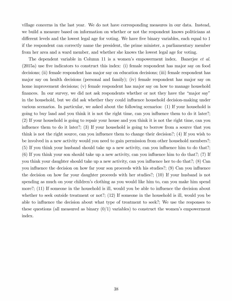
village concerns in the last year. We do not have corresponding measures in our data. Instead,

we build a measure based on information on whether or not the respondent knows politicians at

di¤erent levels and the lowest legal age for voting. We have …ve binary variables, each equal to 1

if the respondent can correctly name the president, the prime minister, a parliamentary member

from her area and a ward member, and whether she knows the lowest legal age for voting.

The dependent variable in Column 11 is a women’s empowerment index. Banerjee et al.

(2015a) use …ve indicators to construct this index: (i) female respondent has major say on food

decisions; (ii) female respondent has major say on education decisions; (iii) female respondent has

major say on health decisions (personal and family); (iv) female respondent has major say on

home improvement decisions; (v) female respondent has major say on how to manage household

…nances. In our survey, we did not ask respondents whether or not they have the “major say”

in the household, but we did ask whether they could in‡uence household decision-making under

various scenarios. In particular, we asked about the following scenarios: (1) If your household is

going to buy land and you think it is not the right time, can you in‡uence them to do it later?;

(2) If your household is going to repair your house and you think it is not the right time, can you

in‡uence them to do it later?; (3) If your household is going to borrow from a source that you

think is not the right source, can you in‡uence them to change their decision?; (4) If you wish to

be involved in a new activity would you need to gain permission from other household members?;

(5) If you think your husband should take up a new activity, can you in‡uence him to do that?;

(6) If you think your son should take up a new activity, can you in‡uence him to do that?; (7) If

you think your daughter should take up a new activity, can you in‡uence her to do that?; (8) Can

you in‡uence the decision on how far your son proceeds with his studies?; (9) Can you in‡uence

the decision on how far your daughter proceeds with her studies?; (10) If your husband is not

spending as much on your children’s clothing as you would like him to, can you make him spend

more?; (11) If someone in the household is ill, would you be able to in‡uence the decision about

whether to seek outside treatment or not?; (12) If someone in the household is ill, would you be

able to in‡uence the decision about what type of treatment to seek?; We use the responses to

these questions (all measured as binary (0/1) variables) to construct the women’s empowerment

index.

38

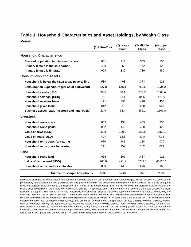
Table 1: Household Characteristics and Asset Holdings, by Wealth Class

Means

(1) Ultra-Poor(2) Near-

Poor

(3) Middle

Class

(4) Upper

Class

Household Characteristics

Share of population in this wealth class .061 .219 .585 .135

Primary female is the sole earner .409 .250 .142 .120

Primary female is illiterate .929 .832 .736 .489

Consumption and Assets

Household is below the $1.25 a day poverty line .530 .493 .373 .121

Consumption Expenditure (per adult equivalent) 627.8 645.1 759.5 1234.2

Household assets [USD] 36.5 68.1 279.9 1663.4

Household savings [USD] 7.9 22.1 84.5 481.9

Household receives loans .191 .393 .498 .433

Household gives loans .012 .018 .030 .067

Business assets (excl. livestock and land) [USD] 22.9 54.4 286.1 1569.8

Livestock

Household owns cows .055 .154 .469 .733

Household owns goats .092 .142 .300 .425

Value of cows [USD] 33.8 120.2 633.8 1559.1

Value of goats [USD] 7.97 12.8 39.8 71.3

Household rents cows for rearing .070 .148 .118 .030

Household rents goats for rearing .111 .157 .102 .021

Land

Household owns land .066 .107 .487 .911

Value of land owned [USD] 200.0 491.2 6789.6 40125.1

Household rents land for cultivation .060 .143 .276 .168

Number of sample households 6732 6743 6328 2036

Notes: All statistics are constructed using baseline household data from both treatment and control villages. Wealth classes are based on the

participatory rural assessment (PRA) exercise: the ultra-poor are ranked in the bottom wealth bins (4th if 4 bins are used, 5th if 5 are used) and

meet the program eligibility criteria, the near-poor are ranked in the bottom wealth bins and do not meet the program eligibility criteria, the

middle class are ranked in the middle wealth bins (2nd and 3rd if 4 are used, 2nd, 3rd and 4th if 5 are used) and the upper classes are those

ranked in the top bin. The number of sample households in each wealth class at baseline is reported at the foot of the table. The poverty line

threshold used is $1.25 per person per day. Consumption expenditure is defined as total household expenditure over the previous year divided

by adult equivalents in the household. The adult equivalence scale gives weight .5 to each child younger than 10. The expenditure items

covered are: food (both purchased and produced), fuel, cosmetics, entertainment, transportation, utilities, clothing, footwear, utensils, textiles,

dowries, education, charity and legal expenses. Household assets include jewelry, sarees, radio, television, mobile phones, furniture, etc.

Household savings refer to value of savings held at home, at any bank, at any MFI and with saving guards. Loans are from both formal and

informal sources. Business assets include pumps, livestock sheds, trees, rickshaws and others. All monetary amounts are PPP-adjusted USD

terms, set at 2007 prices and deflated using CPI published by Bangladesh Bank. In 2007, 1USD=18.46TK PPP.

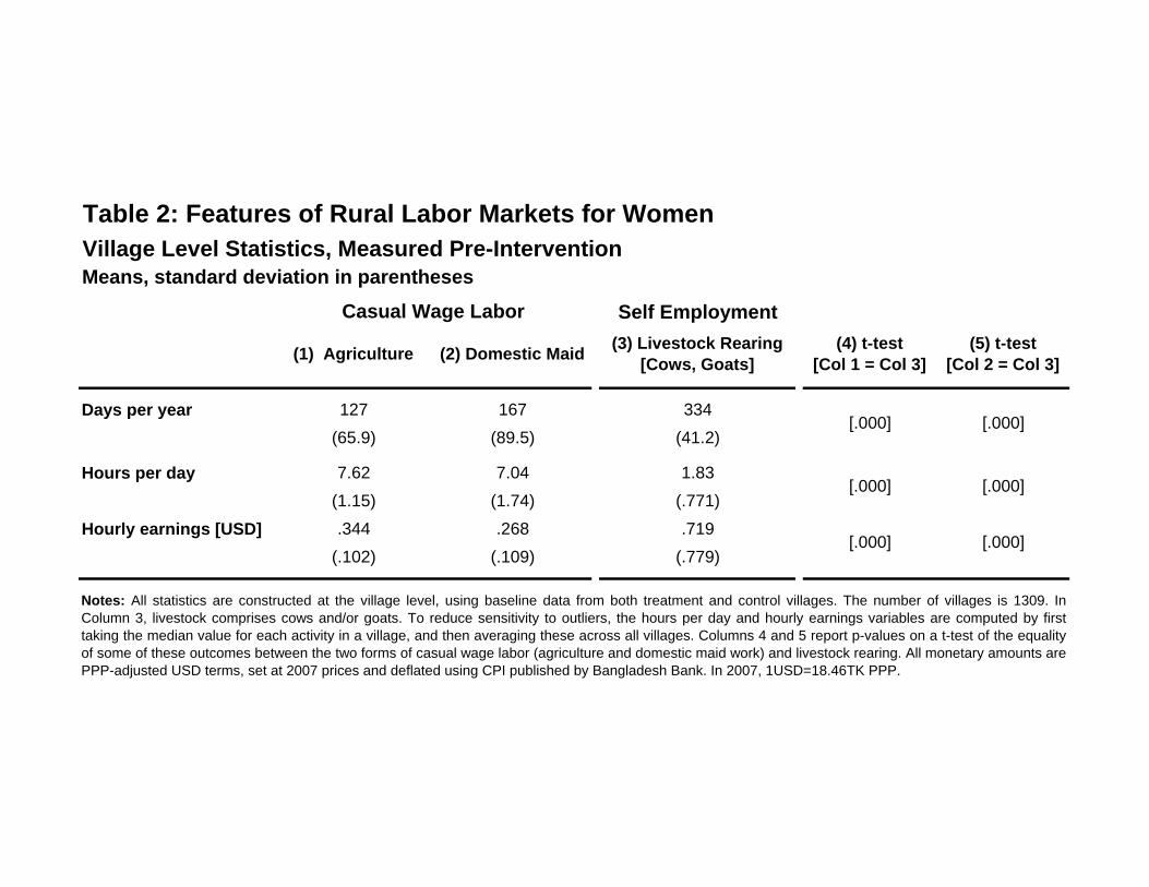
Table 2: Features of Rural Labor Markets for Women

Village Level Statistics, Measured Pre-InterventionMeans, standard deviation in parentheses

Self Employment

(1) Agriculture (2) Domestic Maid(3) Livestock Rearing

[Cows, Goats]

(4) t-test

[Col 1 = Col 3]

(5) t-test

[Col 2 = Col 3]

Days per year 127 167 334

(65.9) (89.5) (41.2)

Hours per day 7.62 7.04 1.83

(1.15) (1.74) (.771)

Hourly earnings [USD] .344 .268 .719

(.102) (.109) (.779)

[.000] [.000]

Notes: All statistics are constructed at the village level, using baseline data from both treatment and control villages. The number of villages is 1309. InColumn 3, livestock comprises cows and/or goats. To reduce sensitivity to outliers, the hours per day and hourly earnings variables are computed by firsttaking the median value for each activity in a village, and then averaging these across all villages. Columns 4 and 5 report p-values on a t-test of the equalityof some of these outcomes between the two forms of casual wage labor (agriculture and domestic maid work) and livestock rearing. All monetary amounts arePPP-adjusted USD terms, set at 2007 prices and deflated using CPI published by Bangladesh Bank. In 2007, 1USD=18.46TK PPP.

Casual Wage Labor

[.000] [.000]

[.000] [.000]

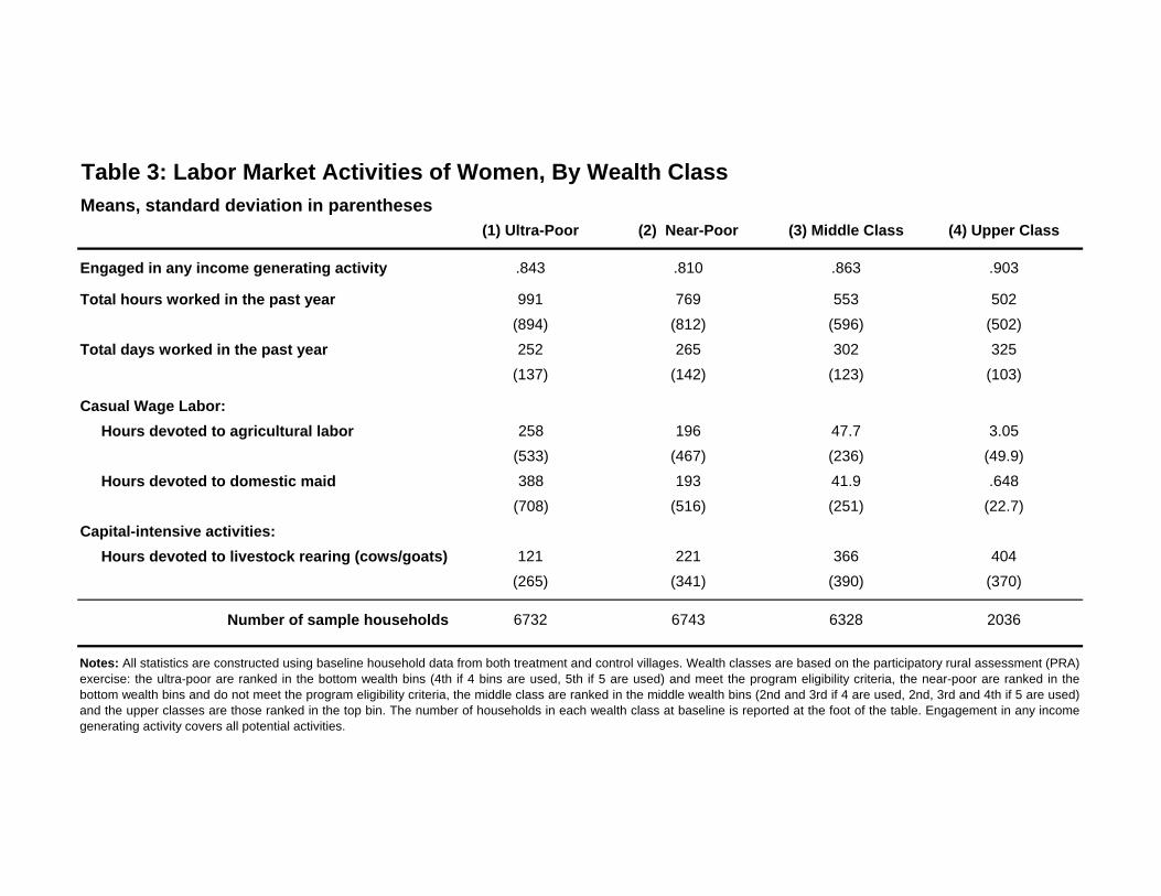
Table 3: Labor Market Activities of Women, By Wealth Class

Means, standard deviation in parentheses

(1) Ultra-Poor (2) Near-Poor (3) Middle Class (4) Upper Class

Engaged in any income generating activity .843 .810 .863 .903

Total hours worked in the past year 991 769 553 502

(894) (812) (596) (502)

Total days worked in the past year 252 265 302 325

(137) (142) (123) (103)

Casual Wage Labor:

Hours devoted to agricultural labor 258 196 47.7 3.05

(533) (467) (236) (49.9)

Hours devoted to domestic maid 388 193 41.9 .648

(708) (516) (251) (22.7)

Capital-intensive activities:

Hours devoted to livestock rearing (cows/goats) 121 221 366 404

(265) (341) (390) (370)

Number of sample households 6732 6743 6328 2036

Notes: All statistics are constructed using baseline household data from both treatment and control villages. Wealth classes are based on the participatory rural assessment (PRA)

exercise: the ultra-poor are ranked in the bottom wealth bins (4th if 4 bins are used, 5th if 5 are used) and meet the program eligibility criteria, the near-poor are ranked in the

bottom wealth bins and do not meet the program eligibility criteria, the middle class are ranked in the middle wealth bins (2nd and 3rd if 4 are used, 2nd, 3rd and 4th if 5 are used)

and the upper classes are those ranked in the top bin. The number of households in each wealth class at baseline is reported at the foot of the table. Engagement in any income

generating activity covers all potential activities.

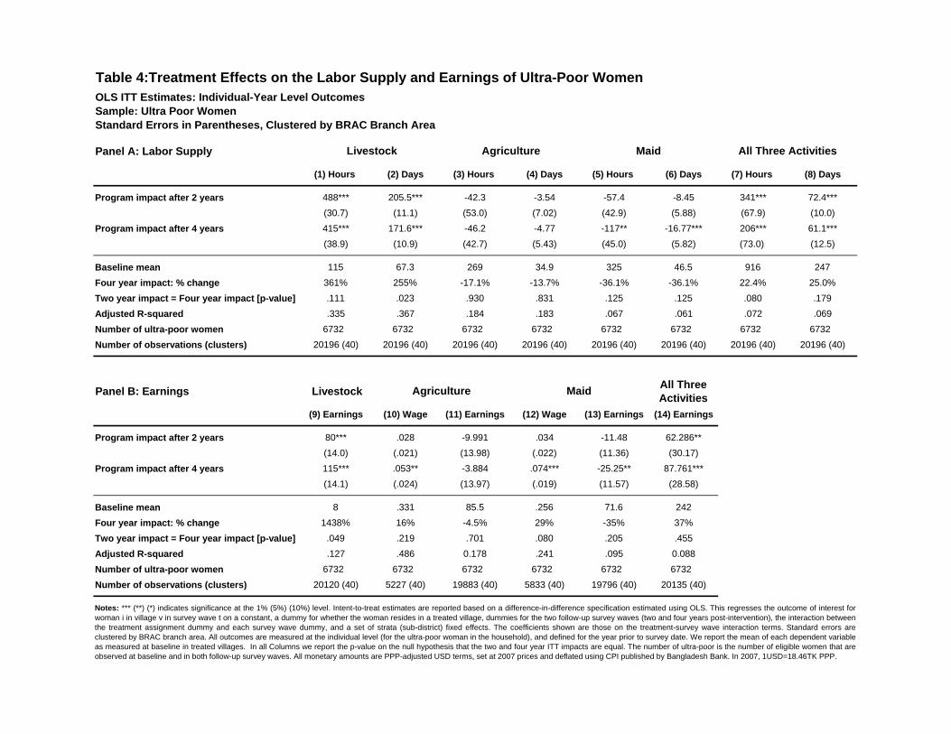
Table 4:Treatment Effects on the Labor Supply and Earnings of Ultra-Poor Women

OLS ITT Estimates: Individual-Year Level Outcomes

Sample: Ultra Poor Women

Standard Errors in Parentheses, Clustered by BRAC Branch Area

Panel A: Labor Supply

(1) Hours (2) Days (3) Hours (4) Days (5) Hours (6) Days (7) Hours (8) Days

Program impact after 2 years 488*** 205.5*** -42.3 -3.54 -57.4 -8.45 341*** 72.4***

(30.7) (11.1) (53.0) (7.02) (42.9) (5.88) (67.9) (10.0)

Program impact after 4 years 415*** 171.6*** -46.2 -4.77 -117** -16.77*** 206*** 61.1***

(38.9) (10.9) (42.7) (5.43) (45.0) (5.82) (73.0) (12.5)

Baseline mean 115 67.3 269 34.9 325 46.5 916 247

Four year impact: % change 361% 255% -17.1% -13.7% -36.1% -36.1% 22.4% 25.0%

Two year impact = Four year impact [p-value] .111 .023 .930 .831 .125 .125 .080 .179

Adjusted R-squared .335 .367 .184 .183 .067 .061 .072 .069

Number of ultra-poor women 6732 6732 6732 6732 6732 6732 6732 6732

Number of observations (clusters) 20196 (40) 20196 (40) 20196 (40) 20196 (40) 20196 (40) 20196 (40) 20196 (40) 20196 (40)

Panel B: Earnings LivestockAll ThreeActivities

(9) Earnings (10) Wage (11) Earnings (12) Wage (13) Earnings (14) Earnings

Program impact after 2 years 80*** .028 -9.991 .034 -11.48 62.286**

(14.0) (.021) (13.98) (.022) (11.36) (30.17)

Program impact after 4 years 115*** .053** -3.884 .074*** -25.25** 87.761***

(14.1) (.024) (13.97) (.019) (11.57) (28.58)

Baseline mean 8 .331 85.5 .256 71.6 242

Four year impact: % change 1438% 16% -4.5% 29% -35% 37%

Two year impact = Four year impact [p-value] .049 .219 .701 .080 .205 .455

Adjusted R-squared .127 .486 0.178 .241 .095 0.088

Number of ultra-poor women 6732 6732 6732 6732 6732 6732

Number of observations (clusters) 20120 (40) 5227 (40) 19883 (40) 5833 (40) 19796 (40) 20135 (40)

Notes: *** (**) (*) indicates significance at the 1% (5%) (10%) level. Intent-to-treat estimates are reported based on a difference-in-difference specification estimated using OLS. This regresses the outcome of interest for

woman i in village v in survey wave t on a constant, a dummy for whether the woman resides in a treated village, dummies for the two follow-up survey waves (two and four years post-intervention), the interaction betweenthe treatment assignment dummy and each survey wave dummy, and a set of strata (sub-district) fixed effects. The coefficients shown are those on the treatment-survey wave interaction terms. Standard errors areclustered by BRAC branch area. All outcomes are measured at the individual level (for the ultra-poor woman in the household), and defined for the year prior to survey date. We report the mean of each dependent variableas measured at baseline in treated villages. In all Columns we report the p-value on the null hypothesis that the two and four year ITT impacts are equal. The number of ultra-poor is the number of eligible women that areobserved at baseline and in both follow-up survey waves. All monetary amounts are PPP-adjusted USD terms, set at 2007 prices and deflated using CPI published by Bangladesh Bank. In 2007, 1USD=18.46TK PPP.

Livestock Agriculture Maid All Three Activities

Agriculture Maid

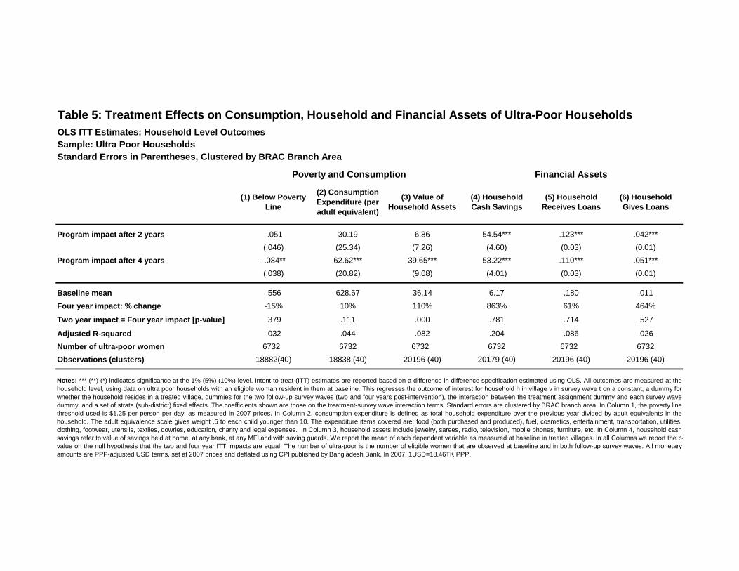
Table 5: Treatment Effects on Consumption, Household and Financial Assets of Ultra-Poor Households

OLS ITT Estimates: Household Level Outcomes

Sample: Ultra Poor Households

Standard Errors in Parentheses, Clustered by BRAC Branch Area

(1) Below Poverty

Line

(2) Consumption

Expenditure (per

adult equivalent)

(3) Value of

Household Assets

(4) Household

Cash Savings

(5) Household

Receives Loans

(6) Household

Gives Loans

Program impact after 2 years -.051 30.19 6.86 54.54*** .123*** .042***

(.046) (25.34) (7.26) (4.60) (0.03) (0.01)

Program impact after 4 years -.084** 62.62*** 39.65*** 53.22*** .110*** .051***

(.038) (20.82) (9.08) (4.01) (0.03) (0.01)

Baseline mean .556 628.67 36.14 6.17 .180 .011

Four year impact: % change -15% 10% 110% 863% 61% 464%

Two year impact = Four year impact [p-value] .379 .111 .000 .781 .714 .527

Adjusted R-squared .032 .044 .082 .204 .086 .026

Number of ultra-poor women 6732 6732 6732 6732 6732 6732

Observations (clusters) 18882(40) 18838 (40) 20196 (40) 20179 (40) 20196 (40) 20196 (40)

Poverty and Consumption Financial Assets

Notes: *** (**) (*) indicates significance at the 1% (5%) (10%) level. Intent-to-treat (ITT) estimates are reported based on a difference-in-difference specification estimated using OLS. All outcomes are measured at the

household level, using data on ultra poor households with an eligible woman resident in them at baseline. This regresses the outcome of interest for household h in village v in survey wave t on a constant, a dummy for

whether the household resides in a treated village, dummies for the two follow-up survey waves (two and four years post-intervention), the interaction between the treatment assignment dummy and each survey wave

dummy, and a set of strata (sub-district) fixed effects. The coefficients shown are those on the treatment-survey wave interaction terms. Standard errors are clustered by BRAC branch area. In Column 1, the poverty line

threshold used is $1.25 per person per day, as measured in 2007 prices. In Column 2, consumption expenditure is defined as total household expenditure over the previous year divided by adult equivalents in the

household. The adult equivalence scale gives weight .5 to each child younger than 10. The expenditure items covered are: food (both purchased and produced), fuel, cosmetics, entertainment, transportation, utilities,

clothing, footwear, utensils, textiles, dowries, education, charity and legal expenses. In Column 3, household assets include jewelry, sarees, radio, television, mobile phones, furniture, etc. In Column 4, household cash

savings refer to value of savings held at home, at any bank, at any MFI and with saving guards. We report the mean of each dependent variable as measured at baseline in treated villages. In all Columns we report the p-

value on the null hypothesis that the two and four year ITT impacts are equal. The number of ultra-poor is the number of eligible women that are observed at baseline and in both follow-up survey waves. All monetary

amounts are PPP-adjusted USD terms, set at 2007 prices and deflated using CPI published by Bangladesh Bank. In 2007, 1USD=18.46TK PPP.

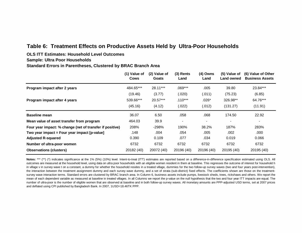
OLS ITT Estimates: Household Level Outcomes

Sample: Ultra Poor Households

Standard Errors in Parentheses, Clustered by BRAC Branch Area

(1) Value ofCows

(2) Value ofGoats

(3) RentsLand

(4) OwnsLand

(5) Value ofLand owned

(6) Value of OtherBusiness Assets

Program impact after 2 years 484.65*** 28.11*** .069*** .005 39.80 23.84***

(19.46) (3.77) (.020) (.011) (75.23) (6.85)

Program impact after 4 years 539.66*** 20.57*** .110*** .026* 326.98** 64.76***

(45.16) (4.12) (.022) (.012) (131.27) (11.91)

Baseline mean 36.07 6.50 .058 .068 174.50 22.92

Mean value of asset transfer from program 464.03 39.9 - - - -

Four year impact: % change (net of transfer if positive) 208% -298% 190% 38.2% 187% 283%

Two year impact = Four year impact [p-value] .148 .004 .054 .005 .002 .000

Adjusted R-squared 0.390 0.109 .077 .034 0.019 0.066

Number of ultra-poor women 6732 6732 6732 6732 6732 6732

Observations (clusters) 20182 (40) 20072 (40) 20196 (40) 20196 (40) 20195 (40) 20195 (40)

Notes: *** (**) (*) indicates significance at the 1% (5%) (10%) level. Intent-to-treat (ITT) estimates are reported based on a difference-in-difference specification estimated using OLS. All

outcomes are measured at the household level, using data on ultra poor households with an eligible women resident in them at baseline. This regresses the outcome of interest for household h

in village v in survey wave t on a constant, a dummy for whether the household resides in a treated village, dummies for the two follow-up survey waves (two and four years post-intervention),

the interaction between the treatment assignment dummy and each survey wave dummy, and a set of strata (sub-district) fixed effects. The coefficients shown are those on the treatment-

survey wave interaction terms. Standard errors are clustered by BRAC branch area. In Column 6, business assets include pumps, livestock sheds, trees, rickshaws and others. We report the

mean of each dependent variable as measured at baseline in treated villages. In all Columns we report the p-value on the null hypothesis that the two and four year ITT impacts are equal. The

number of ultra-poor is the number of eligible women that are observed at baseline and in both follow-up survey waves. All monetary amounts are PPP-adjusted USD terms, set at 2007 prices

and deflated using CPI published by Bangladesh Bank. In 2007, 1USD=18.46TK PPP.

Table 6: Treatment Effects on Productive Assets Held by Ultra-Poor Households

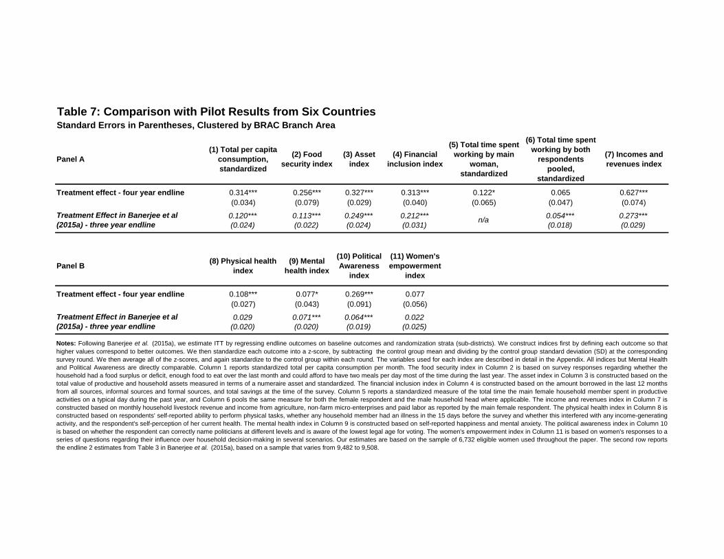
Table 7: Comparison with Pilot Results from Six CountriesStandard Errors in Parentheses, Clustered by BRAC Branch Area

Panel A

(1) Total per capita

consumption,

standardized

(2) Food

security index

(3) Asset

index

(4) Financial

inclusion index

(5) Total time spent

working by main

woman,

standardized

(6) Total time spent

working by both

respondents

pooled,

standardized

(7) Incomes and

revenues index

Treatment effect - four year endline 0.314*** 0.256*** 0.327*** 0.313*** 0.122* 0.065 0.627***

(0.034) (0.079) (0.029) (0.040) (0.065) (0.047) (0.074)

0.120*** 0.113*** 0.249*** 0.212*** 0.054*** 0.273***(0.024) (0.022) (0.024) (0.031) (0.018) (0.029)

Panel B(8) Physical health

index

(9) Mental

health index

(10) Political

Awareness

index

(11) Women's

empowerment

index

Treatment effect - four year endline 0.108*** 0.077* 0.269*** 0.077

(0.027) (0.043) (0.091) (0.056)

0.029 0.071*** 0.064*** 0.022(0.020) (0.020) (0.019) (0.025)

Treatment Effect in Banerjee et al(2015a) - three year endline

n/a

Treatment Effect in Banerjee et al(2015a) - three year endline

Notes: Following Banerjee et al. (2015a), we estimate ITT by regressing endline outcomes on baseline outcomes and randomization strata (sub-districts). We construct indices first by defining each outcome so that

higher values correspond to better outcomes. We then standardize each outcome into a z-score, by subtracting the control group mean and dividing by the control group standard deviation (SD) at the corresponding

survey round. We then average all of the z-scores, and again standardize to the control group within each round. The variables used for each index are described in detail in the Appendix. All indices but Mental Health

and Political Awareness are directly comparable. Column 1 reports standardized total per capita consumption per month. The food security index in Column 2 is based on survey responses regarding whether the

household had a food surplus or deficit, enough food to eat over the last month and could afford to have two meals per day most of the time during the last year. The asset index in Column 3 is constructed based on the

total value of productive and household assets measured in terms of a numeraire asset and standardized. The financial inclusion index in Column 4 is constructed based on the amount borrowed in the last 12 months

from all sources, informal sources and formal sources, and total savings at the time of the survey. Column 5 reports a standardized measure of the total time the main female household member spent in productive

activities on a typical day during the past year, and Column 6 pools the same measure for both the female respondent and the male household head where applicable. The income and revenues index in Column 7 is

constructed based on monthly household livestock revenue and income from agriculture, non-farm micro-enterprises and paid labor as reported by the main female respondent. The physical health index in Column 8 is

constructed based on respondents' self-reported ability to perform physical tasks, whether any household member had an illness in the 15 days before the survey and whether this interfered with any income-generating

activity, and the respondent's self-perception of her current health. The mental health index in Column 9 is constructed based on self-reported happiness and mental anxiety. The political awareness index in Column 10

is based on whether the respondent can correctly name politicians at different levels and is aware of the lowest legal age for voting. The women's empowerment index in Column 11 is based on women's responses to a

series of questions regarding their influence over household decision-making in several scenarios. Our estimates are based on the sample of 6,732 eligible women used throughout the paper. The second row reports

the endline 2 estimates from Table 3 in Banerjee et al. (2015a), based on a sample that varies from 9,482 to 9,508.

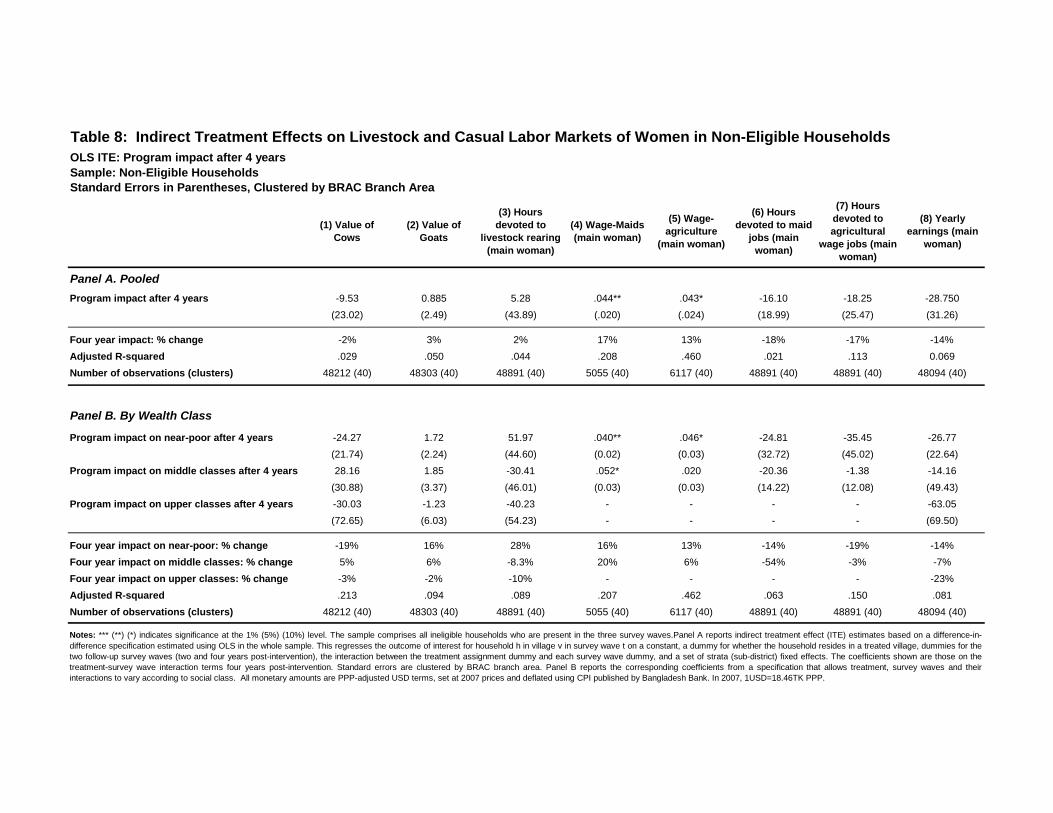
Table 8: Indirect Treatment Effects on Livestock and Casual Labor Markets of Women in Non-Eligible Households

Sample: Non-Eligible Households

Standard Errors in Parentheses, Clustered by BRAC Branch Area

(1) Value of

Cows

(2) Value of

Goats

(3) Hours

devoted to

livestock rearing

(main woman)

(4) Wage-Maids

(main woman)

(5) Wage-

agriculture

(main woman)

(6) Hours

devoted to maid

jobs (main

woman)

(7) Hours

devoted to

agricultural

wage jobs (main

woman)

(8) Yearly

earnings (main

woman)

Panel A. Pooled

Program impact after 4 years -9.53 0.885 5.28 .044** .043* -16.10 -18.25 -28.750

(23.02) (2.49) (43.89) (.020) (.024) (18.99) (25.47) (31.26)

Four year impact: % change -2% 3% 2% 17% 13% -18% -17% -14%

Adjusted R-squared .029 .050 .044 .208 .460 .021 .113 0.069

Number of observations (clusters) 48212 (40) 48303 (40) 48891 (40) 5055 (40) 6117 (40) 48891 (40) 48891 (40) 48094 (40)

Panel B. By Wealth Class

Program impact on near-poor after 4 years -24.27 1.72 51.97 .040** .046* -24.81 -35.45 -26.77

(21.74) (2.24) (44.60) (0.02) (0.03) (32.72) (45.02) (22.64)

Program impact on middle classes after 4 years 28.16 1.85 -30.41 .052* .020 -20.36 -1.38 -14.16

(30.88) (3.37) (46.01) (0.03) (0.03) (14.22) (12.08) (49.43)

Program impact on upper classes after 4 years -30.03 -1.23 -40.23 - - - - -63.05

(72.65) (6.03) (54.23) - - - - (69.50)

Four year impact on near-poor: % change -19% 16% 28% 16% 13% -14% -19% -14%

Four year impact on middle classes: % change 5% 6% -8.3% 20% 6% -54% -3% -7%

Four year impact on upper classes: % change -3% -2% -10% - - - - -23%

Adjusted R-squared .213 .094 .089 .207 .462 .063 .150 .081

Number of observations (clusters) 48212 (40) 48303 (40) 48891 (40) 5055 (40) 6117 (40) 48891 (40) 48891 (40) 48094 (40)

Notes: *** (**) (*) indicates significance at the 1% (5%) (10%) level. The sample comprises all ineligible households who are present in the three survey waves.Panel A reports indirect treatment effect (ITE) estimates based on a difference-in-

difference specification estimated using OLS in the whole sample. This regresses the outcome of interest for household h in village v in survey wave t on a constant, a dummy for whether the household resides in a treated village, dummies for the

two follow-up survey waves (two and four years post-intervention), the interaction between the treatment assignment dummy and each survey wave dummy, and a set of strata (sub-district) fixed effects. The coefficients shown are those on the

treatment-survey wave interaction terms four years post-intervention. Standard errors are clustered by BRAC branch area. Panel B reports the corresponding coefficients from a specification that allows treatment, survey waves and their

interactions to vary according to social class. All monetary amounts are PPP-adjusted USD terms, set at 2007 prices and deflated using CPI published by Bangladesh Bank. In 2007, 1USD=18.46TK PPP.

OLS ITE: Program impact after 4 years

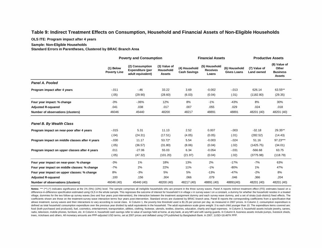
Table 9: Indirect Treatment Effects on Consumption, Household and Financial Assets of Non-Eligible Households

Sample: Non-Eligible HouseholdsStandard Errors in Parentheses, Clustered by BRAC Branch Area

(1) Below

Poverty Line

(2) Consumption

Expenditure (per

adult equivalent)

(3) Value of

Household

Assets

(4) Household

Cash Savings

(5) Household

Receives

Loans

(6) Household

Gives Loans

(7) Value of

Land owned

(8) Value of

Other

Business

Assets

Panel A. Pooled

Program impact after 4 years -.011 -.46 33.22 3.69 -0.002 -.013 626.14 63.55**

(.05) (29.90) (28.60) (6.03) (0.04) (.01) (1182.80) (29.35)

Four year impact: % change -3% -.06% 12% 8% -1% -43% 8% 30%

Adjusted R-squared .041 .038 .017 .007 .055 .029 .024 .018

Number of observations (clusters) 46046 45440 48200 48217 48891 48891 48201 (40) 48201 (40)

Panel B. By Wealth Class

Program impact on near-poor after 4 years -.015 5.31 11.13 2.52 0.007 -.003 -32.18 29.35**

(.04) (24.31) (17.51) (4.05) (0.05) (.01) (282.52) (14.43)

Program impact on middle classes after 4 years -.030 11.17 53.72* 5.54 -0.003 -.024 51.16 97.23***

(.05) (36.57) (31.80) (8.06) (0.04) (.02) (1425.75) (34.01)

Program impact on upper classes after 4 years .011 -27.06 55.03 6.34 -0.054 -.031 -566.68 63.75

(.05) (47.32) (101.20) (21.97) (0.04) (.02) (3775.98) (118.79)

Four year impact on near-poor: % change -3% 1% 18% 13% 2% -17% -7% 63%

Four year impact on middle classes: % change -7% 2% 22% 11% -1% -80% 1% 47%

Four year impact on upper classes: % change 8% -3% 5% 5% -13% -47% -2% 8%

Adjusted R-squared .100 .156 .304 .066 .079 .046 .366 .204

Number of observations (clusters) 46046 (40) 45440 (40) 48200 (40) 48217 (40) 48891 (40) 48891(40) 48201 (40) 48201 (40)

Poverty and Consumption Financial Assets

Notes: *** (**) (*) indicates significance at the 1% (5%) (10%) level. The sample comprises all ineligible households who are present in the three survey waves. Panel A reports indirect treatment effect (ITE) estimates based on a

difference-in-difference specification estimated using OLS in the whole sample. This regresses the outcome of interest for household h in village v in survey wave t on a constant, a dummy for whether the household resides in a treated

village, dummies for the two follow-up survey waves (two and four years post-intervention), the interaction between the treatment assignment dummy and each survey wave dummy, and a set of strata (sub-district) fixed effects. The

coefficients shown are those on the treatment-survey wave interaction terms four years post-intervention. Standard errors are clustered by BRAC branch area. Panel B reports the corresponding coefficients from a specification that

allows treatment, survey waves and their interactions to vary according to social class. In Column 1, the poverty line threshold used is $1.25 per person per day, as measured in 2007 prices. In Column 2, consumption expenditure is

defined as total household consumption expenditure over the previous year divided by adult equivalents in the household. The adult equivalence scale gives weight .5 to each child younger than 10. The expenditure items covered are:

food (both purchased and produced), fuel, cosmetics, entertainment, transportation, utilities, clothing, footwear, utensils, textiles, dowries, education, charity and legal expenses. In Column 3, household assets include jewelry, sarees,

radio, television, mobile phones, furniture, etc. In Column 4, household cash savings refer to value of savings held at home, at any bank, at any MFI and with saving guards. In Column 8, business assets include pumps, livestock sheds,

trees, rickshaws and others. All monetary amounts are PPP-adjusted USD terms, set at 2007 prices and deflated using CPI published by Bangladesh Bank. In 2007, 1USD=18.46TK PPP.

Productive Assets

OLS ITE: Program impact after 4 years

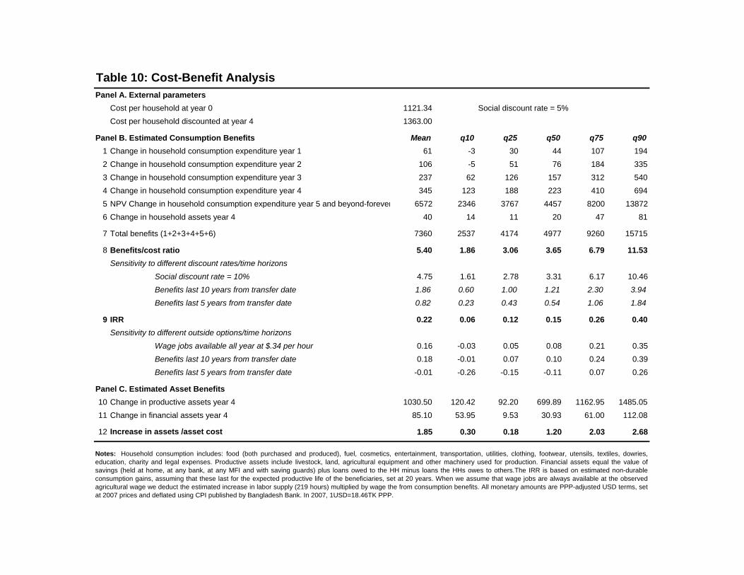
Table 10: Cost-Benefit Analysis

Panel A. External parameters

Cost per household at year 0 1121.34 Social discount rate = 5%

Cost per household discounted at year 4 1363.00

Panel B. Estimated Consumption Benefits Mean q10 q25 q50 q75 q90

1 Change in household consumption expenditure year 1 61 -3 30 44 107 194

2 Change in household consumption expenditure year 2 106 -5 51 76 184 335

3 Change in household consumption expenditure year 3 237 62 126 157 312 540

4 Change in household consumption expenditure year 4 345 123 188 223 410 694

5 NPV Change in household consumption expenditure year 5 and beyond-forever 6572 2346 3767 4457 8200 13872

6 Change in household assets year 4 40 14 11 20 47 81

7 Total benefits (1+2+3+4+5+6) 7360 2537 4174 4977 9260 15715

8 Benefits/cost ratio 5.40 1.86 3.06 3.65 6.79 11.53

Sensitivity to different discount rates/time horizons

Social discount rate = 10% 4.75 1.61 2.78 3.31 6.17 10.46

Benefits last 10 years from transfer date 1.86 0.60 1.00 1.21 2.30 3.94

Benefits last 5 years from transfer date 0.82 0.23 0.43 0.54 1.06 1.84

9 IRR 0.22 0.06 0.12 0.15 0.26 0.40

Sensitivity to different outside options/time horizons

Wage jobs available all year at $.34 per hour 0.16 -0.03 0.05 0.08 0.21 0.35

Benefits last 10 years from transfer date 0.18 -0.01 0.07 0.10 0.24 0.39

Benefits last 5 years from transfer date -0.01 -0.26 -0.15 -0.11 0.07 0.26

Panel C. Estimated Asset Benefits

10 Change in productive assets year 4 1030.50 120.42 92.20 699.89 1162.95 1485.05

11 Change in financial assets year 4 85.10 53.95 9.53 30.93 61.00 112.08

12 1.85 0.30 0.18 1.20 2.03 2.68Increase in assets /asset cost

Notes: Household consumption includes: food (both purchased and produced), fuel, cosmetics, entertainment, transportation, utilities, clothing, footwear, utensils, textiles, dowries,education, charity and legal expenses. Productive assets include livestock, land, agricultural equipment and other machinery used for production. Financial assets equal the value ofsavings (held at home, at any bank, at any MFI and with saving guards) plus loans owed to the HH minus loans the HHs owes to others.The IRR is based on estimated non-durableconsumption gains, assuming that these last for the expected productive life of the beneficiaries, set at 20 years. When we assume that wage jobs are always available at the observedagricultural wage we deduct the estimated increase in labor supply (219 hours) multiplied by wage the from consumption benefits. All monetary amounts are PPP-adjusted USD terms, setat 2007 prices and deflated using CPI published by Bangladesh Bank. In 2007, 1USD=18.46TK PPP.

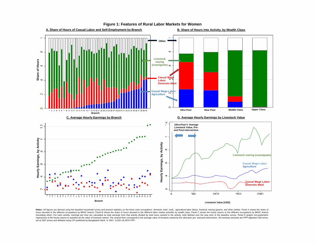
Figure 1: Features of Rural Labor Markets for Women

C. Average Hourly Earnings by Branch D. Average Hourly Earnings by Livestock Value

A. Share of Hours of Casual Labor and Self-Employment by Branch

Notes: All figures are derived using the baseline household survey and present statistics on the three main occupations: domestic maid (red), agricultural labor (blue), livestock rearing (green), and other (white). Panel A shows the share ofhours devoted to the different occupations by BRAC branch. Panel B shows the share of hours devoted to the different labor market activities by wealth class. Panel C shows the hourly returns to the different occupations by BRAC branch(excluding other). For each activity, earnings per hour are calculated as total earnings from that activity divided by total hours worked in the activity, both defined over the year prior to the baseline survey. Panel D graphs non-parametricregressions of the hourly returns to activities by the value of livestock owned. The vertical lines correspond to the average value of livestock owned by the ultra-poor pre- and post-intervention. All monetary amounts are PPP-adjusted USD terms,set at 2007 prices and deflated using CPI published by Bangladesh Bank. In 2007, 1USD=18.46TK PPP.

B. Share of Hours into Activity, by Wealth Class

Livestock Value [USD]

Ultra-Poor's' AverageLivestock Value, Pre-and Post-intervention.

Ho

url

yE

arn

ing

s,

by

Ac

tivit

y

Ho

url

yE

arn

ing

s,

by

Ac

tivit

yS

ha

reo

fH

ou

rs

Casual WageLabor:Domestic Maid

Livestockrearing

(cows/goats)

Casual Wage Labor:Agriculture

Branch

Branch

Livestock rearing (cows/goats)

Casual Wage Labor:Agriculture

Casual Wage Labor:Domestic Maid

Other

Ultra Poor Near Poor Middle Class Upper Class

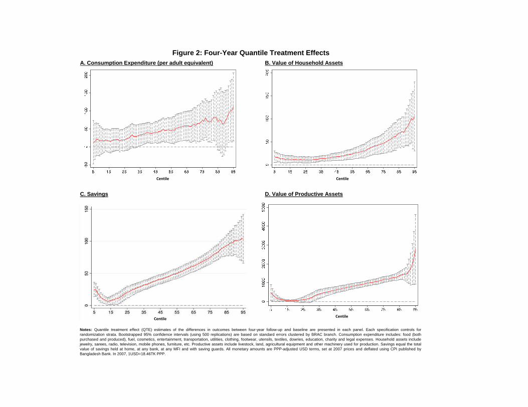
A. Consumption Expenditure (per adult equivalent) B. Value of Household Assets

C. Savings D. Value of Productive Assets

Notes: Quantile treatment effect (QTE) estimates of the differences in outcomes between four-year follow-up and baseline are presented in each panel. Each specification controls forrandomization strata. Bootstrapped 95% confidence intervals (using 500 replications) are based on standard errors clustered by BRAC branch. Consumption expenditure includes: food (bothpurchased and produced), fuel, cosmetics, entertainment, transportation, utilities, clothing, footwear, utensils, textiles, dowries, education, charity and legal expenses. Household assets includejewelry, sarees, radio, television, mobile phones, furniture, etc. Productive assets include livestock, land, agricultural equipment and other machinery used for production. Savings equal the totalvalue of savings held at home, at any bank, at any MFI and with saving guards. All monetary amounts are PPP-adjusted USD terms, set at 2007 prices and deflated using CPI published byBangladesh Bank. In 2007, 1USD=18.46TK PPP.

Figure 2: Four-Year Quantile Treatment Effects

CentileCentile

CentileCentile

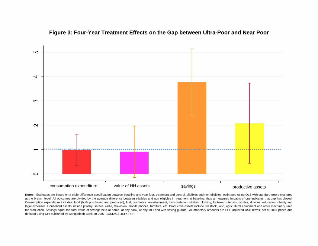
Figure 3: Four-Year Treatment Effects on the Gap between Ultra-Poor and Near Poor

Notes: Estimates are based on a triple-difference specification between baseline and year four, treatment and control, eligibles and non eligibles. estimated using OLS with standard errors clustered

at the branch level. All outcomes are divided by the average difference between eligibles and non eligibles in treatment at baseline, thus a measured impacts of one indicates that gap has closed.

Consumption expenditure includes: food (both purchased and produced), fuel, cosmetics, entertainment, transportation, utilities, clothing, footwear, utensils, textiles, dowries, education, charity and

legal expenses. Household assets include jewelry, sarees, radio, television, mobile phones, furniture, etc. Productive assets include livestock, land, agricultural equipment and other machinery used

for production. Savings equal the total value of savings held at home, at any bank, at any MFI and with saving guards. All monetary amounts are PPP-adjusted USD terms, set at 2007 prices and

deflated using CPI published by Bangladesh Bank. In 2007, 1USD=18.46TK PPP.

consumption expenditure value of HH assets savings productive assets

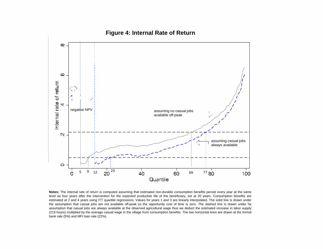
Notes: The internal rate of return is computed assuming that estimated non-durable consumption benefits persist every year at the samelevel as four years after the intervention for the expected productive life of the beneficiary, set at 20 years. Consumption benefits areestimated at 2 and 4 years using ITT quantile regressions. Values for years 1 and 3 are linearly interpolated. The solid line is drawn underthe assumption that casual jobs are not available off-peak so the opportunity cost of time is zero. The dashed line is drawn under heassumption that casual jobs are always available at the observed agricultural wage thus we deduct the estimated increase in labor supply(219 hours) multiplied by the average casual wage in the village from consumption benefits. The two horizontal lines are drawn at the formalbank rate (5%) and MFI loan rate (22%).

Figure 4: Internal Rate of Return

negative NPV assuming no casual jobsavailable off-peak

assuming casual jobsalways available

5 129 2369 77

A. Consumption Expenditure (per adult equivalent) B. Value of Household Assets

C. Savings D. Value of Productive Assets E. Owns or Rents Land

Notes: For each outcome the graphs report estimated changes between baseline and years 2009, 2011, 2014 in treatment and control separately, controlling for sub-district (strata). Vertical bars represent the 95% confidence intervals based on standard errors clustered at the BRAC branch

level. The reported difference in differences estimates are from Tables 5 and 6. Consumption expenditure includes: food (both purchased and produced), fuel, cosmetics, entertainment, transportation, utilities, clothing, footwear, utensils, textiles, dowries, education, charity and legal

expenses. Household assets include jewelry, sarees, radio, television, mobile phones, furniture, etc. Productive assets include livestock, land, agricultural equipment and other machinery used for production. Savings equal the total value of savings held at home, at any bank, at any MFI and

with saving guards. Owns or rents land equals 1 if the individual owns or rents land for cultivation. All monetary amounts are PPP-adjusted USD terms, set at 2007 prices and deflated using CPI published by Bangladesh Bank. In 2007, 1USD=18.46TK PPP.

Figure 5: Yearly Changes in Key Outcomes After 2,4 and 7 years

diff in diff

estimate: 54.5*** diff in diff

estimate:53.2**

diff in diff

estimate: 117*

diff in diff

estimate: 348** diff in diff

estimate: 6.8

diff in diff

estimate:39.6**

diff in diff

estimate:604***

diff in diff

estimate:1030***

diff in diff

estimate:.068***

diff in diff

estimate:.122***

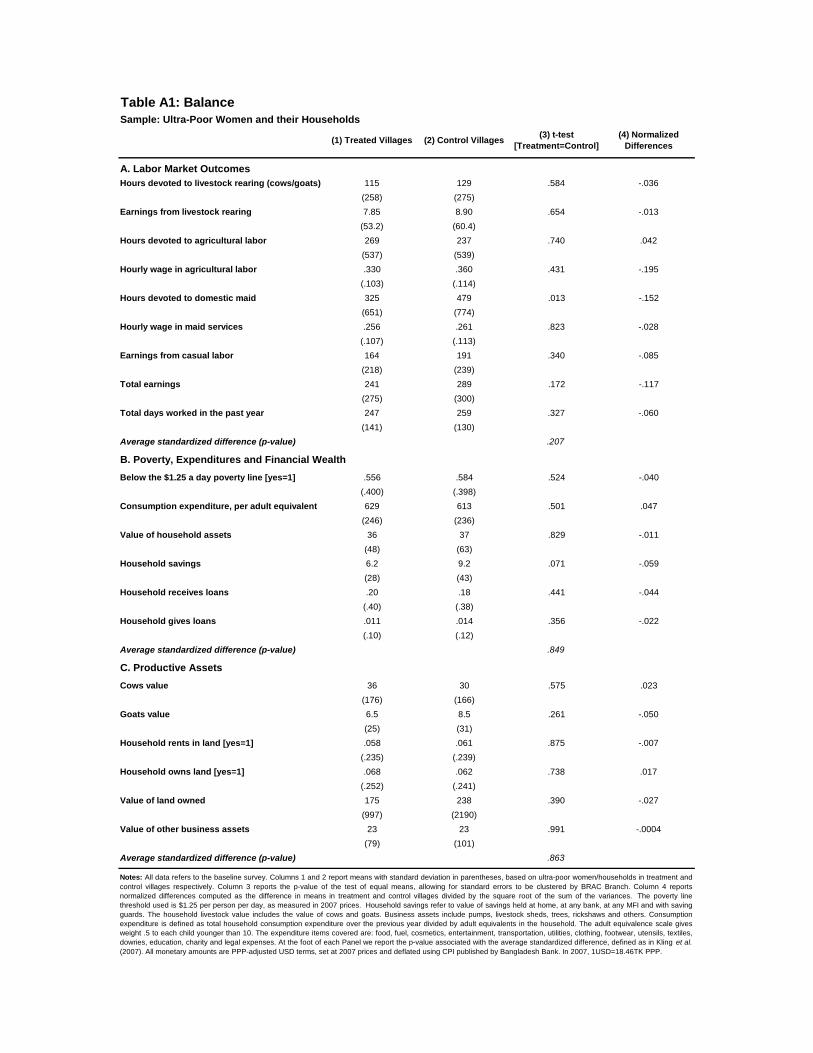
Table A1: BalanceSample: Ultra-Poor Women and their Households

(1) Treated Villages (2) Control Villages(3) t-test

[Treatment=Control]

(4) Normalized

Differences

A. Labor Market Outcomes

Hours devoted to livestock rearing (cows/goats) 115 129 .584 -.036

(258) (275)

Earnings from livestock rearing 7.85 8.90 .654 -.013

(53.2) (60.4)

Hours devoted to agricultural labor 269 237 .740 .042

(537) (539)

Hourly wage in agricultural labor .330 .360 .431 -.195

(.103) (.114)

Hours devoted to domestic maid 325 479 .013 -.152

(651) (774)

Hourly wage in maid services .256 .261 .823 -.028

(.107) (.113)

Earnings from casual labor 164 191 .340 -.085

(218) (239)

Total earnings 241 289 .172 -.117

(275) (300)

Total days worked in the past year 247 259 .327 -.060

(141) (130)

Average standardized difference (p-value) .207

B. Poverty, Expenditures and Financial Wealth

Below the $1.25 a day poverty line [yes=1] .556 .584 .524 -.040

(.400) (.398)

Consumption expenditure, per adult equivalent 629 613 .501 .047

(246) (236)

Value of household assets 36 37 .829 -.011

(48) (63)

Household savings 6.2 9.2 .071 -.059

(28) (43)

Household receives loans .20 .18 .441 -.044

(.40) (.38)

Household gives loans .011 .014 .356 -.022

(.10) (.12)

Average standardized difference (p-value) .849

C. Productive Assets

Cows value 36 30 .575 .023

(176) (166)

Goats value 6.5 8.5 .261 -.050

(25) (31)

Household rents in land [yes=1] .058 .061 .875 -.007

(.235) (.239)

Household owns land [yes=1] .068 .062 .738 .017

(.252) (.241)

Value of land owned 175 238 .390 -.027

(997) (2190)

Value of other business assets 23 23 .991 -.0004

(79) (101)

Average standardized difference (p-value) .863

Notes: All data refers to the baseline survey. Columns 1 and 2 report means with standard deviation in parentheses, based on ultra-poor women/households in treatment and

control villages respectively. Column 3 reports the p-value of the test of equal means, allowing for standard errors to be clustered by BRAC Branch. Column 4 reports

normalized differences computed as the difference in means in treatment and control villages divided by the square root of the sum of the variances. The poverty line

threshold used is $1.25 per person per day, as measured in 2007 prices. Household savings refer to value of savings held at home, at any bank, at any MFI and with saving

guards. The household livestock value includes the value of cows and goats. Business assets include pumps, livestock sheds, trees, rickshaws and others. Consumption

expenditure is defined as total household consumption expenditure over the previous year divided by adult equivalents in the household. The adult equivalence scale gives

weight .5 to each child younger than 10. The expenditure items covered are: food, fuel, cosmetics, entertainment, transportation, utilities, clothing, footwear, utensils, textiles,

dowries, education, charity and legal expenses. At the foot of each Panel we report the p-value associated with the average standardized difference, defined as in Kling et al.

(2007). All monetary amounts are PPP-adjusted USD terms, set at 2007 prices and deflated using CPI published by Bangladesh Bank. In 2007, 1USD=18.46TK PPP.

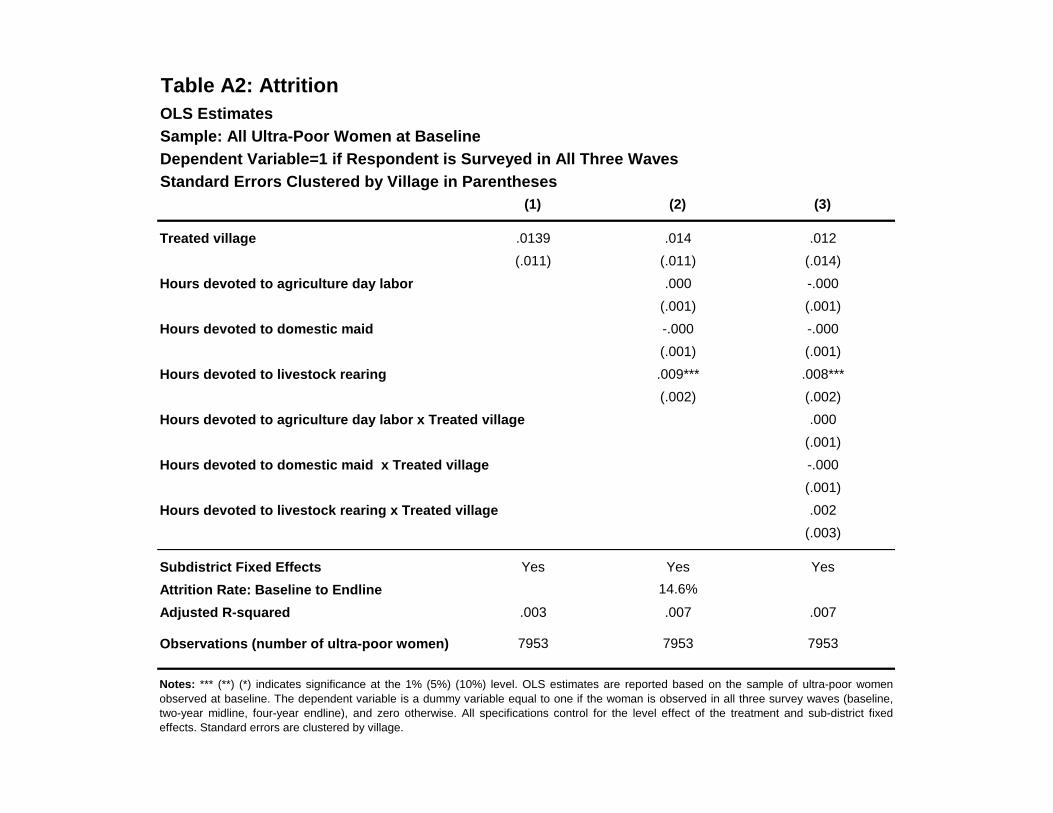
Table A2: Attrition

OLS Estimates

Sample: All Ultra-Poor Women at Baseline

Dependent Variable=1 if Respondent is Surveyed in All Three Waves

Standard Errors Clustered by Village in Parentheses

(1) (2) (3)

Treated village .0139 .014 .012

(.011) (.011) (.014)

Hours devoted to agriculture day labor .000 -.000

(.001) (.001)

Hours devoted to domestic maid -.000 -.000

(.001) (.001)

Hours devoted to livestock rearing .009*** .008***

(.002) (.002)

Hours devoted to agriculture day labor x Treated village .000

(.001)

Hours devoted to domestic maid x Treated village -.000

(.001)

Hours devoted to livestock rearing x Treated village .002

(.003)

Subdistrict Fixed Effects Yes Yes Yes

Attrition Rate: Baseline to Endline

Adjusted R-squared .003 .007 .007

Observations (number of ultra-poor women) 7953 7953 7953

Notes: *** (**) (*) indicates significance at the 1% (5%) (10%) level. OLS estimates are reported based on the sample of ultra-poor women

observed at baseline. The dependent variable is a dummy variable equal to one if the woman is observed in all three survey waves (baseline,two-year midline, four-year endline), and zero otherwise. All specifications control for the level effect of the treatment and sub-district fixedeffects. Standard errors are clustered by village.

14.6%

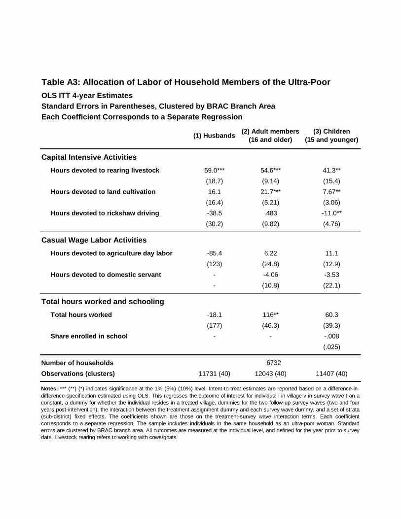
Table A3: Allocation of Labor of Household Members of the Ultra-Poor

OLS ITT 4-year Estimates

Standard Errors in Parentheses, Clustered by BRAC Branch Area

Each Coefficient Corresponds to a Separate Regression

(1) Husbands(2) Adult members

(16 and older)

(3) Children

(15 and younger)

Capital Intensive Activities

Hours devoted to rearing livestock 59.0*** 54.6*** 41.3**

(18.7) (9.14) (15.4)

Hours devoted to land cultivation 16.1 21.7*** 7.67**

(16.4) (5.21) (3.06)

Hours devoted to rickshaw driving -38.5 .483 -11.0**

(30.2) (9.82) (4.76)

Casual Wage Labor Activities

Hours devoted to agriculture day labor -85.4 6.22 11.1

(123) (24.8) (12.9)

Hours devoted to domestic servant - -4.06 -3.53

- (10.8) (22.1)

Total hours worked and schooling

Total hours worked -18.1 116** 60.3

(177) (46.3) (39.3)

Share enrolled in school - - -.008

(.025)

Number of households

Observations (clusters) 11731 (40) 12043 (40) 11407 (40)

6732

Notes: *** (**) (*) indicates significance at the 1% (5%) (10%) level. Intent-to-treat estimates are reported based on a difference-in-

difference specification estimated using OLS. This regresses the outcome of interest for individual i in village v in survey wave t on a

constant, a dummy for whether the individual resides in a treated village, dummies for the two follow-up survey waves (two and four

years post-intervention), the interaction between the treatment assignment dummy and each survey wave dummy, and a set of strata

(sub-district) fixed effects. The coefficients shown are those on the treatment-survey wave interaction terms. Each coefficient

corresponds to a separate regression. The sample includes individuals in the same household as an ultra-poor woman. Standard

errors are clustered by BRAC branch area. All outcomes are measured at the individual level, and defined for the year prior to survey

date. Livestock rearing refers to working with cows/goats.

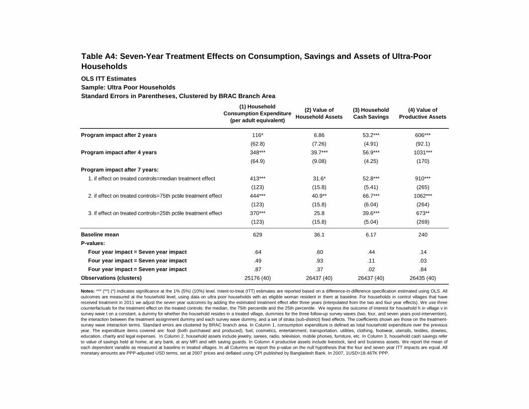
OLS ITT Estimates

Sample: Ultra Poor Households

Standard Errors in Parentheses, Clustered by BRAC Branch Area

(1) Household

Consumption Expenditure

(per adult equivalent)

(2) Value of

Household Assets

(3) Household

Cash Savings

(4) Value of

Productive Assets

Program impact after 2 years 116* 6.86 53.2*** 606***

(62.8) (7.26) (4.91) (92.1)

Program impact after 4 years 348*** 39.7*** 56.9*** 1031***

(64.9) (9.08) (4.25) (170)

Program impact after 7 years:

1. if effect on treated controls=median treatment effect 413*** 31.6* 52.8*** 910***

(123) (15.8) (5.41) (265)

2. if effect on treated controls=75th pctile treatment effect 444*** 40.9** 66.7*** 1062***

(123) (15.8) (6.04) (264)

3. if effect on treated controls=25th pctile treatment effect 370*** 25.8 39.6*** 673**

(123) (15.8) (5.04) (269)

Baseline mean 629 36.1 6.17 240

P-values:

Four year impact = Seven year impact .64 .60 .44 .14

Four year impact = Seven year impact .49 .93 .11 .03

Four year impact = Seven year impact .87 .37 .02 .84

Observations (clusters) 25176 (40) 26437 (40) 26437 (40) 26435 (40)

Notes: *** (**) (*) indicates significance at the 1% (5%) (10%) level. Intent-to-treat (ITT) estimates are reported based on a difference-in-difference specification estimated using OLS. All

outcomes are measured at the household level, using data on ultra poor households with an eligible woman resident in them at baseline. For households in control villages that have

received treatment in 2011 we adjust the seven year outcomes by adding the estimated treatment effect after three years (interpolated from the two and four year effects). We use three

counterfactuals for the treatment effect on the treated controls: the median, the 75th percentile and the 25th percentile. We regress the outcome of interest for household h in village v in

survey wave t on a constant, a dummy for whether the household resides in a treated village, dummies for the three follow-up survey waves (two, four, and seven years post-intervention),

the interaction between the treatment assignment dummy and each survey wave dummy, and a set of strata (sub-district) fixed effects. The coefficients shown are those on the treatment-

survey wave interaction terms. Standard errors are clustered by BRAC branch area. In Column 1, consumption expenditure is defined as total household expenditure over the previous

year. The expenditure items covered are: food (both purchased and produced), fuel, cosmetics, entertainment, transportation, utilities, clothing, footwear, utensils, textiles, dowries,

education, charity and legal expenses. In Column 2, household assets include jewelry, sarees, radio, television, mobile phones, furniture, etc. In Column 3, household cash savings refer

to value of savings held at home, at any bank, at any MFI and with saving guards. In Column 4 productive assets include livestock, land and business assets. We report the mean of

each dependent variable as measured at baseline in treated villages. In all Columns we report the p-value on the null hypothesis that the four and seven year ITT impacts are equal. All

monetary amounts are PPP-adjusted USD terms, set at 2007 prices and deflated using CPI published by Bangladesh Bank. In 2007, 1USD=18.46TK PPP.

Table A4: Seven-Year Treatment Effects on Consumption, Savings and Assets of Ultra-Poor

Households

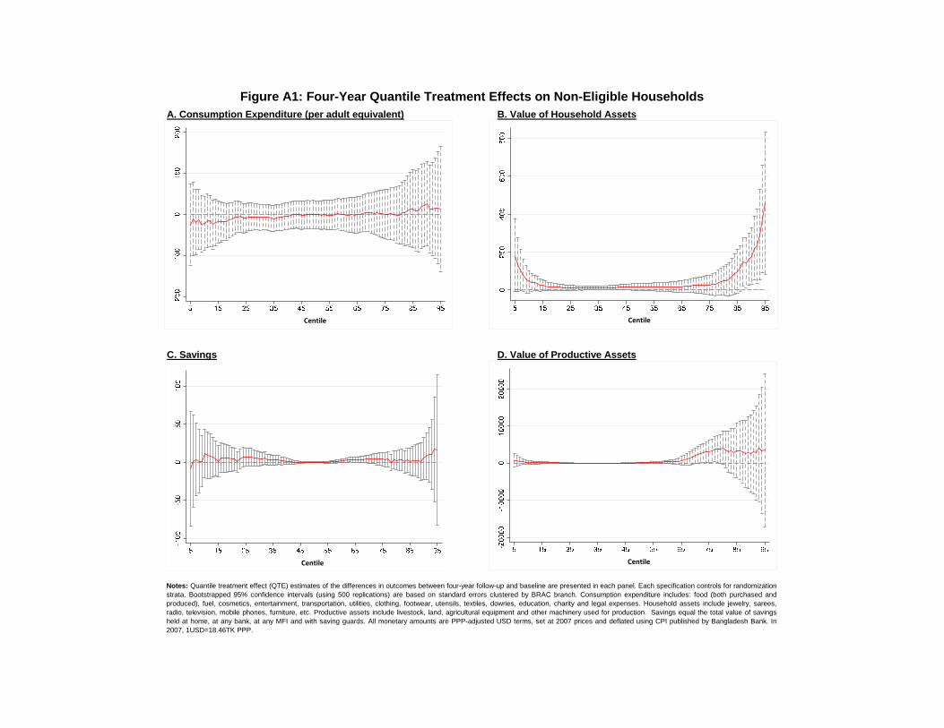
A. Consumption Expenditure (per adult equivalent) B. Value of Household Assets

C. Savings D. Value of Productive Assets

Figure A1: Four-Year Quantile Treatment Effects on Non-Eligible Households

Notes: Quantile treatment effect (QTE) estimates of the differences in outcomes between four-year follow-up and baseline are presented in each panel. Each specification controls for randomization

strata. Bootstrapped 95% confidence intervals (using 500 replications) are based on standard errors clustered by BRAC branch. Consumption expenditure includes: food (both purchased and

produced), fuel, cosmetics, entertainment, transportation, utilities, clothing, footwear, utensils, textiles, dowries, education, charity and legal expenses. Household assets include jewelry, sarees,

radio, television, mobile phones, furniture, etc. Productive assets include livestock, land, agricultural equipment and other machinery used for production. Savings equal the total value of savings

held at home, at any bank, at any MFI and with saving guards. All monetary amounts are PPP-adjusted USD terms, set at 2007 prices and deflated using CPI published by Bangladesh Bank. In

2007, 1USD=18.46TK PPP.

Centile

CentileCentile

Centile