Lab 1 - Path Models, Indirect Effects, and Single Indicator FactorsStructural Equation Modeling ED 216F - Instructor: Karen Nylund-Gibson

Adam Garber

April 03, 2020

DATA SOURCE: This lab exercise utilizes the NCES public-use dataset: Education Longitu-dinal Study of 2002 (Lauff & Ingels, 2014) See website: nces.ed.gov

Tools for reproducibility:

Tool/Package Purpose/Utility Advantages{MplusAutomation} package Current capabilities supporting full SEM modeling High flexibilityR Project Unbreakable file paths & neatness Reproducibility (kindness to your future self){tidyverse} package Intuitive/descriptive function names Accessibility to new users{here} package Unbreakable/consistent file paths across OS Reproducibility (for Science’s sake!){haven} package View-able metadata in R from SPSS data-files Getting to know your measures{ggplot2} package Clear, customizable, reproducible figures Publication quality data visualizationspipe operator (%>%) notation Ease of reading/writing scripts e.g., first() %>% and_then() %>% and_finally()

1

Creating a version-controlled R-Project by downloading repository from Github

Download ropository here: https://github.com/garberadamc/SEM-Lab1

Create a class folder (to save labs and assignments)

a. click “NEW PROJECT” (upper right corner of window)b. choose option Version Controlc. choose option Gitd. paste the repository web URL path coppied from the clone or download button on the repo pagee. choose location of the R-Project (too many nested folders will result in filepath error)

Create sub-folders within the project folder. In R-studio under the files pane . . .

a. click “New Folder” and name folder “data”b. click “New Folder” and name folder “mplus_files”c. click “New Folder” and name folder “figures”

Install the “rhdf5” package to read gh5 files

if (!requireNamespace("BiocManager", quietly = TRUE))install.packages("BiocManager")

BiocManager::install("rhdf5")

Load packages

library(MplusAutomation)library(haven)library(rhdf5)library(tidyverse)library(here)library(corrplot)library(kableExtra)library(reshape2)library(janitor)library(ggridges)library(DiagrammeR)library(semPlot)library(sjPlot)

Keyboard shortcuts

• ALT + DASH(-) = <-• SHIFT + CONTROL = %>%

2

Read in SPSS data

spss_data <- read_spss(here("data", "els_sub1_spss.sav")) %>%janitor::clean_names() # makes all variable names lowercase

Preparations: subset, rename, and reorder columns

1. subset: select columns in 3 ways, remove columns with (-), select by index number, and select bycolumn name

2. rename: change variable names to be descriptive and within the Mplus 8 character limit3. reorder: this makes it easy to choose sequential variables for {MplusAutomation}

spss_sub0 <- spss_data %>%select(-stu_id, -sch_id, -byrace,

-byparace, -byparlng, -byfcomp,-bypared, -bymothed, -byfathed,-bysctrl, -byurban, -byregion)

Select the first 9 columns (by index) and select the next 17 columns (by name)

spss_sub1 <- spss_sub0 %>%select(1:9,

bys20a, bys20h, bys20j, bys20k, bys20m, bys20n,bys21b, bys21d, bys22a, bys22b, bys22c, bys22d,bys22e, bys22g, bys22h, bys24a, bys24b) %>%

rename("stu_exp" = "bystexp", # "NEW_NAME" = "OLD_NAME""par_asp" = "byparasp","mth_read" = "bytxcstd","mth_test" = "bytxmstd","rd_test" = "bytxrstd","freelnch" = "by10flp","stu_tch" = "bys20a","putdownt" = "bys20h","unsafe" = "bys20j","disrupt" = "bys20k","gangs" = "bys20m","rac_fght" = "bys20n","fair" = "bys21b","strict" = "bys21d","stolen" = "bys22a","drugs" = "bys22b","t_hurt" = "bys22c","p_fight" = "bys22d","hit" = "bys22e","damaged" = "bys22g","bullied" = "bys22h","late" = "bys24a","skipped" = "bys24b")

3

More housekeeping: reorder columns

spss_sub2 <- spss_sub1 %>%select(

bystlang, # dichotomous (yes,no)freelnch, byincome, # ordinal (binned, continuous scale)stolen, t_hurt, p_fight, hit, damaged, bullied, # ordinal frequency (3-point)unsafe, disrupt, gangs, rac_fght, # ordinal Likert (4-point scale)late, skipped, # ordinal frequency (4-point scale)mth_test, rd_test) # continuous (standardized test scores)

Make a codebook including metadata using ‘sjPlot‘

sjPlot::view_df(spss_sub2)

Types of data for different tasks

• SAV (e.g., spss_data.sav): this data format is for SPSS files & contains variable labels (meta-data)• CSV (e.g., r_ready_data.csv): this is the preferable data format for reading into R (no labels)• DAT (e.g., mplus_data.dat): this is the data format used to read into Mplus (no column names or

strings)

NOTE: Mplus also accepts TXT formatted data (e.g., mplus_data.txt)

Converting data between 3 formats: writing and reading data

Write a CSV datafile (preferable format for reading into R, with SPSS labels removed)

write_csv(spss_sub2, here("data", "els_sub6_data.csv"))

Write a SPSS datafile (preferable format for reading into SPSS, labels are preserved)

write_sav(spss_sub2, here("data", "els_sub6_data.sav"))

Read the unlabeled data back into R

tidy_data <- read_csv(here("data", "els_sub6_data.csv"))

Write a DAT datafile for Mplus (this function removes header row & converts missing values to non-string)

4

prepareMplusData(tidy_data, here("data", "els_sub6_data.dat"))

Make a ‘tribble‘ table

var_table <- tribble(~"Name", ~"Labels", ~"Value Labels (limit)",

#-----------|-----------------------------------------------|--------------------------------------|,"bystlang" , "Whether English is students native language" ,"0=No, 1=Yes","freelnch" , "Grade 10 percent free lunch-categorical" ,"0=0-5%, 7=76-100%","byincome" , "Total family income from all sources 2001" ,"1=None, 13=$200,001 or more","stolen" , "Had something stolen at school" ,"1=Never, 3=More than twice","t_hurt" , "Someone threatened to hurt 10th grader at school","1=Never, 3=More than twice","p_fight" , "Got into a physical fight at school" ,"1=Never, 3=More than twice" ,"hit" , "Someone hit 10th grader" ,"1=Never, 3=More than twice" ,"damaged" , "Someone damaged belongings" ,"1=Never, 3=More than twice" ,"bullied" , "Someone bullied or picked on 10th grader" ,"1=Never, 3=More than twice" ,"unsafe" , "Does not feel safe at this school" ,"1=Strongly agree, 4=Strongly disagree" ,"disrupt" , "Disruptions get in way of learning" ,"1=Strongly agree, 4=Strongly disagree" ,"gangs" , "There are gangs in school" ,"1=Strongly agree, 4=Strongly disagree" ,"rac_fght" , "Racial-ethnic groups often fight" ,"1=Strongly agree, 4=Strongly disagree" ,"late" , "How many times late for school" ,"1=Never, 4=10 or more times" ,"skipped" , "How many times cut-skip classes" ,"1=Never, 4=10 or more times" ,"mth_test" , "Math test standardized score" ,"0-100" ,"rd_test" , "Reading test standardized score" ,"0-100" ,

)

var_table %>%kable("latex", booktabs = T, linesep = "") %>%kable_styling(latex_options = c("striped"),

full_width = F,position = "left")

5

Name Labels Value Labels (limit)bystlang Whether English is students native language 0=No, 1=Yesfreelnch Grade 10 percent free lunch-categorical 0=0-5%, 7=76-100%byincome Total family income from all sources 2001 1=None, 13=$200,001 or morestolen Had something stolen at school 1=Never, 3=More than twicet_hurt Someone threatened to hurt 10th grader at school 1=Never, 3=More than twicep_fight Got into a physical fight at school 1=Never, 3=More than twicehit Someone hit 10th grader 1=Never, 3=More than twicedamaged Someone damaged belongings 1=Never, 3=More than twicebullied Someone bullied or picked on 10th grader 1=Never, 3=More than twiceunsafe Does not feel safe at this school 1=Strongly agree, 4=Strongly disagreedisrupt Disruptions get in way of learning 1=Strongly agree, 4=Strongly disagreegangs There are gangs in school 1=Strongly agree, 4=Strongly disagreerac_fght Racial-ethnic groups often fight 1=Strongly agree, 4=Strongly disagreelate How many times late for school 1=Never, 4=10 or more timesskipped How many times cut-skip classes 1=Never, 4=10 or more timesmth_test Math test standardized score 0-100rd_test Reading test standardized score 0-100

Take a look at the data - some practice with ‘ggplot2‘

Make a facetted box plot

# some formatting, add labels to `bystlang` for plottidy_data <- tidy_data %>%

mutate(bystlang = factor(bystlang,labels = c(`0` = "Non-English", `1` = "English")))

ggplot(data=drop_na(tidy_data), aes(y=mth_test)) +geom_boxplot() +facet_wrap(~bystlang) +labs(x = "Native language",

y = "Math test (standardized score)")

6

Non−English English

−0.4 −0.2 0.0 0.2 0.4−0.4 −0.2 0.0 0.2 0.4

40

60

80

Native language

Mat

h te

st (

stan

dard

ized

sco

re)

Make a density plot

ggplot(data=drop_na(tidy_data), aes(x=mth_test)) +geom_density(aes(fill = bystlang),

color = NA,show.legend = FALSE) +

facet_wrap(~bystlang) +theme_light()

7

Non−English English

40 60 80 40 60 80

0.00

0.01

0.02

0.03

0.04

mth_test

dens

ity

Ridgeline plot {ggridges}

# A ridgeline plot is good way to compare distributions across groups.# In the plot below the distribution of reading test scores is grouped# by level of the freelunch variable.

ridge_graph <- ggplot(data = drop_na(tidy_data),aes(x = rd_test, y = factor(freelnch))) +

geom_density_ridges(aes(fill = factor(freelnch)),size = 0.2,alpha = 0.7,show.legend = FALSE) +

scale_x_continuous(lim = c(0,100)) +scale_y_discrete(lim = levels(tidy_data$freelnch),

labels = c("0-5%", "6-10%", "11-20%","21-30%","31-50%", "51-75%", "76-100%")) +

labs(x = "Reading test (standardized score)",y = "Percent Free Lunch",

title = "Grade 10 Reading Test Scores by Percent Free Lunch in School",subtitle = "Source: ElS 2002") +theme_minimal()

ridge_graph

8

0−5%

6−10%

11−20%

21−30%

31−50%

51−75%

76−100%

0 25 50 75 100Reading test (standardized score)

Per

cent

Fre

e Lu

nch

Source: ElS 2002

Grade 10 Reading Test Scores by Percent Free Lunch in School

Look at all bivariate relations

t_cor <- cor(tidy_data[,4:17], use = "pairwise.complete.obs")

corrplot(t_cor,method = "color",type = "upper",tl.col="black",tl.srt=45)

9

−1

−0.8

−0.6

−0.4

−0.2

0

0.2

0.4

0.6

0.8

1stolen

t_hu

rt

p_fig

ht

hit dam

aged

bullie

d

unsa

fe

disru

pt

gang

s

rac_

fght

late

skipp

ed

mth

_tes

t

rd_t

est

stolen

t_hurt

p_fight

hit

damaged

bullied

unsafe

disrupt

gangs

rac_fght

late

skipped

mth_test

rd_test

Run some path models with MplusAutomation

Practice run, use type=basic to get descriptives

m_basic <- mplusObject(TITLE = "RUN TYPE = BASIC ANALYSIS - LAB 1",VARIABLE =

" ! an mplusObject() will always need a 'usevar' statement! ONLY specify variables that will be used in analysis! lines of code in MPLUS ALWAYS end with a semicolon ';'

usevar =bystlang freelnch byincome stolen t_hurt p_fighthit damaged bullie, unsafe disrupt gangs rac_fghtlate skipped mth_test rd_test;",

ANALYSIS ="type = basic" ,

MODEL = "" ,

PLOT = "",

10

OUTPUT = "",

usevariables = colnames(tidy_data), # tell MplusAutomation the column names to userdata = tidy_data) # this is the data object used (must be un-label)

m_basic_fit <- mplusModeler(m_basic,dataout=here("mplus_files", "Lab1.dat"),modelout=here("mplus_files", "m0_basic_Lab1.inp"),check=TRUE, run = TRUE, hashfilename = FALSE)

Run a path model with model indirect (to estimate the indirect effect)

Figure 1. Path Diagram of Multiple Indirect Paths Model

Visualize the path diagram using the {DiagrammeR} package

mermaid("graph LR

bystlang-->latebystlang-->skippedbystlang-->mth_testlate-->skippedlate-->mth_testskipped-->mth_test

")

11

Run model depicted above with multiple indirect paths

m1_ind <- mplusObject(TITLE = "m1 model indirect - Lab 1",VARIABLE ="usevar =bystlang ! covariatelate skipped ! mediatorsmth_test; ! outcome ",

ANALYSIS ="estimator = MLR" ,

MODEL ="late on bystlang ;skipped on late bystlang ;mth_test on late skipped bystlang;

Model indirect:mth_test ind bystlang;mth_test via late skipped bystlang; " ,

OUTPUT = "sampstat standardized",

usevariables = colnames(tidy_data),rdata = tidy_data)

m1_ind_fit <- mplusModeler(m1_ind,dataout=here("mplus_files", "Lab1.dat"),

modelout=here("mplus_files", "m1_indirect_Lab1.inp"),check=TRUE, run = TRUE, hashfilename = FALSE)

Generate a path diagram from Mplus output with {semPlot}

order2_model <- readModels(here("mplus_files","m1_indirect_Lab1.out"))

# plot model:semPaths(order2_model,

intercepts=FALSE)

Single indicator factors

Model specifications:

• Fix the loading to 1

12

• Then fix the residual variance to a specific value (you are not estimating a measurement parameter)

Using reliability you fix the residual variance at:

(1 − reliabilty) ∗ variance

Lab example of single indicator factor model:

Figure 2. Path Diagram of Single Indicator Factor Model

create a mean score variable called mean_score

tidy_data2 <- tidy_data %>%mutate(mean_scr = rowSums(select(., late:skipped))/2)

- Reliability = .8 (set to)- Variance = .77 (mean_score)

Function to fix the residual variance

13

# r = reliability, v = variance

resid_var <- function(r,v) {

y <- ((1-r)*v)return(y)

}

y01 <- resid_var(.8,.77)

print(y01)

## [1] 0.154

Run model with single indicator factor

m2_sif <- mplusObject(TITLE = "m2 single indicator factor - Lab 1",VARIABLE ="usevar =unsafe disrupt gangs rac_fght ! factor 1mth_test ! outcomemean_scr; ! mediator ",

ANALYSIS ="estimator = MLR" ,

MODEL ="! measurement modelfactor1 by unsafe, disrupt, gangs, rac_fght;

SIF by mean_scr@1; ! fix factor loading to 1

mean_scr@.154; ! fix residual variance

! structural modelmth_test on factor1 SIF;SIF on factor1; ",

OUTPUT = "sampstat standardized",

usevariables = colnames(tidy_data2),rdata = tidy_data2)

m2_sif_fit <- mplusModeler(m2_sif,dataout=here("mplus_files", "Lab1.dat"),

modelout=here("mplus_files", "m2_sif_Lab1.inp"),check=TRUE, run = TRUE, hashfilename = FALSE)

14

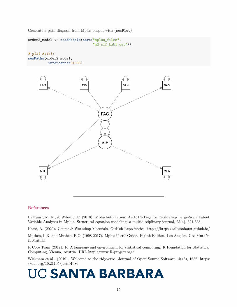
Generate a path diagram from Mplus output with {semPlot}

order2_model <- readModels(here("mplus_files","m2_sif_Lab1.out"))

# plot model:semPaths(order2_model,

intercepts=FALSE)

References

Hallquist, M. N., & Wiley, J. F. (2018). MplusAutomation: An R Package for Facilitating Large-Scale LatentVariable Analyses in Mplus. Structural equation modeling: a multidisciplinary journal, 25(4), 621-638.

Horst, A. (2020). Course & Workshop Materials. GitHub Repositories, https://https://allisonhorst.github.io/

Muthén, L.K. and Muthén, B.O. (1998-2017). Mplus User’s Guide. Eighth Edition. Los Angeles, CA: Muthén& Muthén

R Core Team (2017). R: A language and environment for statistical computing. R Foundation for StatisticalComputing, Vienna, Austria. URL http://www.R-project.org/

Wickham et al., (2019). Welcome to the tidyverse. Journal of Open Source Software, 4(43), 1686, https://doi.org/10.21105/joss.01686

15