arX

iv:1

903.

0697

4v1

[cs

.SY

] 1

6 M

ar 2

019

Prescribed-time convergence with input constraints: A control

Lyapunov function based approach

Kunal Garg Ehsan Arabi Dimitra Panagou

Abstract— In this paper, we present a control frameworkfor a general class of control-affine nonlinear systems underspatiotemporal and input constraints. Specifically, the proposedcontrol architecture addresses the problem of reaching a givenfinal set S in a prescribed (user-defined) time with boundedcontrol inputs. To this end, a time transformation technique isutilized to transform the system subject to temporal constraintsinto an equivalent form without temporal constraints. Thetransformation is defined so that asymptotic convergence in thetransformed time scale results into prescribed-time convergencein the original time scale. To incorporate input constraints, wecharacterize a set of initial conditions DM such that startingfrom this set, the closed-loop trajectories reach the set S withinthe prescribed time. We further show that starting from outsidethe set DM , the system trajectories reach the set DM in a finitetime that depends upon the initial conditions and the controlinput bounds. We use a novel parameter µ in the controller, thatcontrols the convergence-rate of the closed-loop trajectories anddictates the size of the set DM . Finally, we present a numericalexample to showcase the efficacy of our proposed method.

I. INTRODUCTION

In many real-world applications, various types of con-

straints are present due to the structural and operational

requirements of the considered system. For example, spatial

constraints are common in safety-critical applications. There

are a lot of studies on forward invariance of sets where the

objective is to design a control law such that the closed-

loop system trajectories are contained in a given set for

all times. Some examples include: [1], where a Lyapunov-

like barrier function based approach is utilized to guarantee

asymptotic tracking, as well as ensuring that the system

output always remains inside a given set; [2], [3], where

conditions using zeroing barrier functions are presented to

ensure forward invariance of a desired set. The authors of

[4] present sufficient conditions in terms of existence of a

barrier certificate for forward invariance of a given set, and

propose a sum-of-squares formulation to find the certificate.

In addition to spatial constraints, temporal constraints

appear in time-critical applications where completion of a

task is required upon a given time instance. The concept

of finite-time stability (FTS) has been studied to ensure

convergence of solutions in finite time. In the seminal work

[5], the authors introduce necessary and sufficient conditions

in terms of a Lyapunov function for continuous, autonomous

systems to exhibit FTS. Fixed-time stability (FxTS) [6] is a

The authors are with the Department of Aerospace Engineering,University of Michigan, Ann Arbor, MI, USA; {kgarg, earabi,

dpanagou}@umich.edu.The authors would like to acknowledge the support of the Air Force

Office of Scientific Research under award number FA9550-17-1-0284.

stronger notion than FTS, where the time of convergence

does not depend upon the initial conditions. Prescribed-time

stability, or user-defined time stability or strongly predefined-

time stability [7]–[9], imposes that the convergence time

can be chosen arbitrarily. The authors of [7], [10] study

a time transformation approach to stretch the finite-time

domain of interest [0, T ) to an infinite-time domain [0,∞).With a proper choice of the transformation, the asymptotic

convergence in the new stretched time domain inherently

implies the finite-time convergence at the prescribed time

T in the original time domain (see also [11]–[14] for more

details). Input constraints, such as actuator saturation, is an-

other class of constraints that is inevitable in practice. Since

a limited control input can affect the region of fixed-time

convergence, addressing spatiotemporal and input constraints

simultaneously is a challenging control problem.

In contrast to the forward invariance problem, the problem

of reaching a user-defined set deals with designing a control

law such that the closed-loop system trajectories, starting

from outside some set S, reach the set S in a given time.

When the set S contains only the equilibrium, then reaching

the set S reduces to the regular point stabilization problem.

Control synthesis for the problem of reaching a general

set S has received much attention. A recent result in [15]

introduces the notion of FTS of closed sets for hybrid

dynamical systems. The authors of [16] formulate a quadratic

program to ensure finite-time convergence to a set with

input constraints. Although they consider input bounds, the

approach does not yield closed-form controllers. Under the

traditional notion of FTS, as defined in [5], the convergence

time in [15], [16] depends upon the initial conditions.

In this paper, we study the problem of reaching a given

set in a prescribed-time T for a general class of control-

affine systems with input constraints. We present sufficient

conditions for reaching a general set S = {x | h(x) ≤ 0}in time T . We present novel sufficient conditions in terms

of existence of a CLF to guarantee existence of a controller

that derives the closed-loop trajectories to the set S.

In contrast to the results in [16], we propose a control

law in closed-form. Furthermore, in contrast to the results in

[15], the closed-loop system trajectories resulting from our

controller reach the given set in a prescribed-time that can be

chosen arbitrarily and independently of the initial conditions

in the absence of input constraints. To incorporate input

constraints, we then characterize a set of initial conditions

DM starting from which, the closed-loop trajectories reach

the set S in the prescribed time T . As expected, assigning

an arbitrary prescribed convergence time for any initial

condition may not be possible in the presence of actuator

saturation. To this end, we derive a lower bound on the

prescribed time of convergence T , so that the control input

remains bounded at all times. When the initial conditions

of the system are outside the set DM , we show that the

proposed controller yields convergence to the set DM within

a finite time that depends on the initial conditions and the

control input bounds. We use a novel tuning parameter µ in

the controller and show how the size of the set DM and the

convergence rate can be adjusted based on the value of this

parameter.

The rest of the paper is organized as follows. Section II

presents the notation used in the paper and some mathe-

matical preliminaries. In Section III, we detail the controller

design and present the main results of the paper. In Section

IV, we present a numerical example to explain the various

aspects of the proposed method and we conclude the paper

with our thoughts for future work in Section V.

II. MATHEMATICAL PRELIMINARIES

In the rest of the paper, R denotes the set of real numbers,

R+ denotes the set of non-negative real numbers, Rn denotes

the set of n×1 real column vectors, and f(T−) (respectively,

f(T+)) denotes the left (respectively, the right) limit of the

function f at T . In addition, we write bd(S) for the boundary

of the closed set S, and ‖x‖S = infy∈S ‖x − y‖ for the

distance of the point x /∈ S from the set S. A function α :R+ → R+ is said to belong to class-K, denoted as α ∈ K,

if α(0) = 0 and α is strictly increasing. The Lie derivative

of a function V : Rn → R along a vector field f : Rn → Rn

at a point x ∈ Rn is denoted as LfV , ∂V

∂x f(x).

Next, we introduce the notion of prescribed-time stability.

Consider a nonlinear system given by

x(t) = f(x(t)), x(0) = x0, (1)

where x ∈ Rn and f : Rn → R

n is continuous with f(0) =0. The origin is said to be an FTS equilibrium of (1) if

it is Lyapunov stable and finite-time convergent, i.e., for all

x(0) ∈ N \{0}, where N is some open neighborhood of the

origin, limt→T x(t) = 0, where T = T (x(0)) < ∞ depends

upon the initial condition x(0) [5]. The authors in [6] define

the notion of FxTS, where the time of convergence does not

depend upon the initial condition. The following notion of

prescribed-time stability allows the time of convergence Tto be chosen a priori.

Definition 1 ( [7]–[9]): The origin of (1) is called as

prescribed-time stable if the trajectories of (1) reach the

origin in time T < ∞, where T > 0 is a user defined

constant.

We introduce a time transformation technique for con-

verting a user-defined time interval of interest [0, T ) into

a stretched infinite-time interval [0,∞) [7], [10], [11]. Con-

sider the function θ : R+ → R+ defined as

t = θ(s), (2)

where t ∈ [0, T ), s ∈ [0,∞), and the function θ(s) satisfies

θ(0) = 0, θ′(0) = 1, (3a)

s1 > s2 ≥ 0 =⇒ θ(s1) > θ(s2), (3b)

lims→∞

θ(s) = T, lims→∞

θ′(s) = 0. (3c)

We need (3a) to ensure continuity of the proposed controller,

(3b) implies that θ(s) is strictly increasing, while (3c) is

needed to ensure that asymptotic convergence in s results

into prescribed time convergence in t. A candidate time

transformation function satisfying (3) is given by

t = θ(s) , T (1− e−sT ), (4)

where T > 0 is the user-defined finite time.

Remark 1 ( [17] Section 1.1.1.4): Let ξ(t) denote a solu-

tion to the dynamical system

x(t) = f(t, x(t)), x(0) = x0. (5)

Let t = θ(s) satisfy (3), and define χ(s) = ξ(t) so that

χ′(s) = θ′(s)f(θ(s), χ(s)), χ(θ−1(0)) = x0, (6)

where χ′(s) , dχ(s)/ds, θ′(s) , dθ(s)/ds and

lims→∞ χ(s) = limt→T ξ(t).Remark 2: For the sake of simplicity, considering the time

transformation t = θ(s) and any signal η(t), we write ηs(s)to denote the signal η(t) in the transformed time coordinate

s, i.e., ηs(s) , η(θ(s)).

III. PRESCRIBED-TIME CONTROL DESIGN

Consider the system

x(t) = f(x) + g(x)u(t), x(0) = x0, (7)

where x(t) ∈ Rn is the system state vector, f : Rn → R

n,

g : Rn → Rn and u ∈ R is the control input. The problem

statement is as follows.

Problem 1: Design the control input u(t) so that

• The closed-loop trajectories of (7) reach the set S ={x | h(x) ≤ 0} for a given function h : Rn → R in a

user-defined time T , i.e., ∀t ≥ T and ∀x0 ∈ D ⊂ Rn,

x(t) ∈ S;

• For a user-defined control bound uM > 0, u satisfies

−uM ≤ u(t) ≤ uM , ∀ t ≥ 0. (8)

First, we utilize the time transformation given in (2) to

represent the system dynamics in (7) in the new stretched

infinite time interval [0,∞). From Remarks 1 and 2, we

obtain

x′s(s) = f(s, xs(s)) + g(s, xs(s))us(s), (9)

where xs(s) = x(t), xs(θ−1(0)) = x0, f(s, x) = f(x)θ′(s)

and g(s, x) = g(x)θ′(s). We now re-state Problem 1 in the

new time-scale for (9).

Problem 2: Design the control input us(s) such that

• The closed-loop trajectories of (9) reach the set S ={x | h(x) ≤ 0} for a given function h : Rn → R asymp-

totically, i.e., ∀xs(0) ∈ D ⊂ Rn, lims→∞ xs(s) ∈ S;

• The control input satisfies

−uM ≤ us(s) ≤ uM , ∀ s ≥ 0, (10)

for a user-defined control bound uM > 0.

The control Lyapunov function (CLF) is defined as fol-

lows.

Definition 2 ( [18]): A continuously differentiable, posi-

tive definite function V : Rn → R is called CLF for (7) if

for all t ≥ 0 it satisfies

infu{LfV (x(t)) + LgV (x(t))u} ≤ 0, (11)

We make the following assumption for system (7).

Assumption 1: There exists a CLF V for (7).

Remark 3: In contrast to [16], where the authors use the

function h(x) as the CLF, Assumption 1 is more general

and gives more freedom to choose the CLF as some function

other than h(x). It also allows more general class of set Sthat can be considered since we do not need the function

h(x) to be continuously differentiable.

From Definition 2, V is positive definite. Using [19,

Lemma 4.3], there exist α1, α2 ∈ K such that:

α1(‖x‖S) ≤ V (x) ≤ α2(‖x‖S), ∀x. (12)

Now, we present the controller for (9) so that its trajecto-

ries reach the set S asymptotically. Define the functions a, bas

a(s, xs) = LfV (xs), b(s, xs) = LgV (xs). (13)

Also, define the functions a0, b0 as

a0(xs) = LfV (xs), b0(xs) = LgV (xs). (14)

Note that for time-invariant functions f, g, the functions

a0, b0 are also time invariant. From (13) and (14), we have

a0(xs) =1

θ′(s)a(s, xs), b0(xs) =

1

θ′(s)b(s, xs). (15)

Using (13) and inspired from Sontag’s formula [18], we

define the control signal u(·) as

u(θ′(s), xs(s)) =

−a+ µ

θ′(s)

√

a2+ b4

(θ′(s))2

b , b 6= 0,

0, b = 0,

(16)

where µ > 0 is a tuning parameter (see Remark 7 for details

on how to choose this parameter). In order to incorporate

input constraints (10), define the set D0 as

D0 = {x | |u(·, ·)| ≤ uM}. (17)

Remark 4: The system (9) is a time-varying system, hence,

a stabilizing feedback law for time-invariant system (7) does

not necessarily stabilize (9) (see [20] for details).

Lemma 1: Along the closed-loop trajectories of (9) with

us = u, the CLF V satisfies:

V ′(xs) ,dV (xs)

ds= −µ

√

a0(xs)2 + b0(xs)4, (18)

for all xs such that b(s, xs(s)) 6= 0.

Proof: For xs such that b 6= 0, the control input is

given as u = −(

a+ µθ′(s)

√

a2 + b4

(θ′(s))2

)

/b. The derivative

of V along the closed-loop trajectories of (9) results in

V ′ = LfV + LgV u = a+ b

−a+ µ

θ′(s)

√

a2 + b4

(θ′(s))2

b

,

= −µ

√

( a

θ′(s)

)2

+( b

(θ′(s))

)4 (15)= −µ

√

a20 + b40.

We make the following assumptions.

Assumption 2: There exist positive constants k1, k2, l such

that the following hold for all x ∈ D1 ⊂ Rn:

‖a0(x)‖ =∥

∥

∥

∂V

∂xf(x)

∥

∥

∥ ≤ l‖x‖2S, (19a)

k1‖x‖S ≤ ‖b0(x)‖ =∥

∥

∥

∂V

∂xg(x)

∥

∥

∥ ≤ k2‖x‖S , (19b)

where D1 is an open set containing S.

Note that (19b) implies that

W (x) ,√

a0(x)2 + b0(x)4 ≥ c‖x‖2S , (20)

where c = k21 , for all x ∈ D1 ⊂ Rn.

Assumption 3: There exist c1, c2 > 0 such that

c1‖x‖2S ≤ α1(‖x‖S), (21a)

α2(‖x‖S) ≤ c2‖x‖2S, (21b)

for all x ∈ D2 ⊂ Rn, D2 is an open set containing S.

Remark 5: Similar assumptions have been used in liter-

ature previously. Authors in [21] use these assumptions to

define an exponentially stabilizing CLF (ES-CLF); [22] uses

(21) to show asymptotic stability; [23] uses (20) in the

definition of CLF (see [24, Remark 5] as well).

We state the following results on boundedness and conti-

nuity of u.

Lemma 2: The following holds for some k > 0, for all

s ≥ 0

|u(θ′(s), xs(s))| ≤ k

√

V0

c1e(

1T− µc

2c2)s. (22)

Additionally, if T > 2c2µc , then lims→∞ u = 0.

Proof: See Appendix I.

In what follows, we assume that T > 2c2µc . Define

DM = {x | V (x) ≤ c1

(uM

k

)2

}, (23)

and m2 = µc2c2

, so that for x0 ∈ DM , we have

|u| ≤ k

√

V0

c1e−m2s+s/T ≤ k

√

V0

c1≤ uM .

Note that DM ⊆ D0 where D0 is defined as in (17). We

propose the control input as

u(t) =

u(θ′(θ−1(t− TM )), x(t)), x(t) ∈ DM ,

u(1, x(t)), x(t) ∈ D0 \DM ,

uMu(1,x(t))|u(1,x(t))| , x(t) /∈ D0,

(24)

where TM is the time instant when the trajectories of (7)

enter the set DM , i.e., x(TM ) ∈ bd(DM ) and x(t) /∈ DM

for all t < TM , and

u(y, x) =

−a0(x)+µy

√a0(x)2+b0(x)4

b0(x), b0(x) 6= 0,

0, b0(x) = 0.(25)

From (25), we obtain that

u(1, x) = −a0(x) + µ√

a0(x)2 + b0(x)4

b0(x),

which is time-invariant and depends only on x. Note that

the time transformation technique is utilized only within the

set DM , i.e., t = TM + θ(s) and we have s = 0 when the

system trajectories of (7) enter the set DM at t = TM .

Lemma 3: The control input u(t) defined as (24) is con-

tinuous and satisfies the control input constraints (8).

Proof: See Appendix II.

We divide the problem in two parts:

• In Theorem 1, we show that for x(0) ∈ DM , the closed

loop trajectories reach the set S in time T .

• In Theorem 2, we show that if x(0) /∈ DM , then the

closed loop trajectories of (7) reach the set DM in a

finite time T0(x0) + T1.

Define D = D1

⋂

D2, where D1 is defined in Assumption

2, and D2 is defined in Assumption 3.

Theorem 1: Under the effect of control input (24), the

trajectories of (7) reach the set S in the prescribed time

T for all xs(0) ∈ DM

⋂

D.

Proof: Based on (12), V (xs) = 0 implies ‖xs‖S = 0.

So, it is sufficient to prove that V (xs(s)) = 0 as s → 0.

Now, for xs ∈ bd(DM ), it follows from (18), (20) and (21)

that V ′(xs) ≤ − cc2V (xs) < 0. Hence, we obtain that the

set DM is forward-invariant. This implies that xs(s) ∈ DM

for all s ≥ 0. From (24), we have u(t) = u(θ′(s), xs) for

xs ∈ DM and hence, V ′(xs) ≤ − cc2V (xs) holds for all

s ≥ 0. Therefore, lims→∞ V (xs(s)) = 0, which in turn

implies that lims→∞ ‖xs(s)‖S = limt→T ‖x(t)‖S = 0.

Remark 6: Based on (23), the set DM grows larger as the

input bound uM increases. So, for larger input bounds, the

set of initial conditions, from which the trajectories converge

to the set S in the prescribed time, is larger.

Theorem 2: If x0 /∈ DM , then the closed-loop trajectories

of (7) reach the set DM in a finite-time T0(x0) + T1 for

all x0 ∈ D⋂

D where D = {x | ‖x‖S ≤ µcuMc1lc2k

}. If, in

addition, x0 ∈ D0 \DM , then T0(x0) = 0.

Proof: Consider the case when x0 /∈ D0. From (24), we

have u(t) = uMu(1,x)|u(1,x)| . The time derivative V (x(t)) reads

V = a0 + b0u = a0 − b0uM

|u(1, x)|a0 + µ

√

a20 + b40b0

= a0 −uM

|u(1, x)| (a0 + µ√

a20 + b40)

= a0(1−uM

|u(1, x)| )−uMµ

|u(1, x)|√

a20 + b40.

Now, if a0 < 0, we obtain that a0(

1 − uM

|u(1,x)|)

< 0 since

|u(1, x)| > uM . Using this, we obtain

V ≤ − uMµ

|u(1, x)|√

a20 + b40(20)

≤ −cµuM

|u(1, x)| ‖x‖2S

(33)

≤ −cµuM

k‖x‖‖x‖2S = −δµ‖x‖S , (26)

where k =(

l(1 + µ)/k1+µk2)

and δ = cuM/k. Now, using

(12), (21) and (26), we obtain

V ≤ −γV12 , (27)

where γ = µδc− 1

22 . Define V = min

x∈bd(D0)V (x). Now, since

x0 /∈ D0, we know that V (x(0)) > V . Denote t = T such

that V (x(T )) = V . From (27), using Comparison lemma

[19, Lemma 3.4], we obtain that

V (0)12 − V

12 ≥ 1

2γT =⇒ T ≤ 2(V (0)

12 − V

12 )

γ.

For the case when a0 > 0, we have

V = a0(1−uM

|u(1, x)| )−uMµ

|u(1, x)|√

a20 + b40

(19)

≤ l‖x‖2 − uMµ

|u(1, x)|√

a20 + b40

(27)

≤ l‖x‖2 − γV12

(21)

≤ l

c1V − γV

12 .

Now, for x0 ∈ D = {x | ‖x‖S ≤ γc1l√c2}, we know that l

c1V−

γV12 < 0. Using [25, Lemma 1], we obtain that for all x0 ∈

D, there exists a finite time T (x0), such that V (x(T )) =0, which implies that there exists a time T (x0) such that

V (x(T )) = V . Choose T0(x0) = max{T (x0), T (x0)} so

that for all x0 ∈ D, the trajectories of (7) reach the set D0

in time T0(x0).Once the trajectories reach D0, the control input is defined

as u(t) = u(1, x), so the inequality (31) holds. Let xmax =max

x∈bd(D0)‖x‖S . Using (31), we obtain

‖x(t+ T0)‖ ≤ m1e−m2t =

√

V (T0)

c1e−m2t

(21)

≤√

c2‖x(T0)‖2c1

e−m2t ≤√

c2c1

e−m2txmax.

(28)

Let t = T0 + T1 be the time instant when the trajectories

of (7) enter the set DM , i.e., x(T0 + T1) ∈ bd(DM ) and

x(t) /∈ DM for all t < T0 + T1. From (23), we know that

x ∈ bd(DM ) =⇒ ‖x‖S ≤ uM

k

(

c1c2

)12

. Using this and (28),

we obtain

uM

k

(c1c2

)12 ≤

√

c2c1e−m2txmax =⇒ t ≥

log(

c1c2

uM

k

)

logm2,

which implies that for all t ≥log

(

c1c2

uMkxmax

)

logm2, x(t) ∈ DM .

Since the above analysis computes the worst case time to

reach the set DM , i.e., starting from xmax, we obtain that

T1 ≤log

(

c1c2

uMkxmax

)

logm2. Hence, for any x0 ∈ D, the closed-

loop trajectories of (7) reach the set DM in a finite-time

T0(x0) + T1. Since T0(x0) is the time required to reach the

set D0, we obtain that if x0 ∈ D0, then T0(x0) = 0.

Note that T0 + T1, i.e., the time of convergence to the set

DM , depends upon the initial condition x(0) and the control

bound uM . Now we can state the main result of the paper.

Theorem 3: Under the effect of control input (24), the

closed-loop trajectories of (7) reach the set S in a finite

time T ≤ T + T0(x0) + T1 for all x0 ∈ D⋂

D, where T is

the user-defined time as in Problem 1.

Proof: It follows from Theorem 1 that for x(0) ∈ DM ,

the closed-loop trajectories reach the set S in the prescribed

time T . From Theorem 2, we obtain that for x(0) /∈ DM ,

the closed-loop trajectories reach the set D0 in time T0(x0)and from D0, the closed-loop trajectories reach the set DM

in time T1. Hence, we have that for all t ≥ T , where T ≤T + T0(x0) + T1, x(t) ∈ S for all x(0) ∈ D

⋂

D.

Remark 7: Note that constant k = l(1+µ)k1

+ µk2 in the

definition of set DM decreases as the tuning parameter µdecreases. Hence, for smaller values of µ, the set DM is

larger. On the other hand, the parameter γ in the definition

of set D is such that γ ∝ µl(1+µ)/k1+µk2

. So, γ decreases

with µ, and saturates to the maximum value γ∞ = 1l/k1+k2

as µ increases. Hence, the set D shrinks as µ decreases and

saturates as µ grows larger. On the basis of these trade-offs,

the user can choose appropriate value of µ, depending upon

requirements on the sets DM and D for a given problem.

IV. NUMERICAL EXAMPLE

We consider the following system:

x1 = x2 + x1(x21 + x2

2 − 1) + x1u,

x2 = −x1 + ζ(x2)(x21 + x2

2 − 1) + x2u,

where ζ(x) = (0.8 + 0.2e−100|x|) tanh(x) and the set Sdefined as S = {x | ‖x‖ ≤ 1}. Note that in the absence of

the control input, the trajectories diverge away from the set

S, i.e., the set S is unstable for the open-loop system. We

choose uM = 7, µ = 0.05 and use V = 12 (x

21 + x2

2 − 1)2. In

addition, we set T = 5 seconds for the time transformation

function in (4). With ‖x‖S = x21+x2

2−r2, Assumptions 2, 3

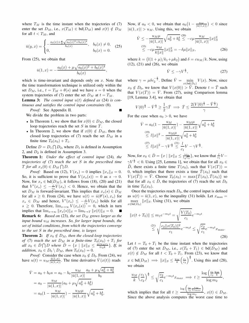
are satisfied. Figures 1 and 2 respectively show the closed-

loop system trajectories and the control input for different

initial conditions. In Figure 1, the set D0 is denoted with red

dashed-line and set DM is denoted with black dotted-line.

Figure 3 shows the variation of control Lyapunov function

V with time. The control Lyapunov function drops to 1e−15

within 5 sec for the case when x(0) ∈ DM and within 5.5

sec for the other cases. One can see from these figures that

the system trajectories reach the set S with bounded control

input u(t) ∈ [−uM , uM ] within the prescribed finite time

T = 5 seconds when x(0) ∈ DM and within a finite time

greater than 5 sec when x(0) /∈ DM .

We use log-scale to plot V (t) with time, so that the

variation of the function is clear when the values are very

-3 -2 -1 0 1 2 3 4

-2

-1

0

1

2

3

4

Fig. 1. Closed-loop system trajectories for different initial conditions.

Fig. 2. Control input signal u(t) for the system trajectories in Figure 1.

small. Also, note that unlike asymptotic convergence, which

is plotted as a straight line on the log-scale, the control

Lyapunov functions drops super-linearly from 1e−3 to 1e−15.

This verifies the finite-time convergence nature of the pro-

posed controller.

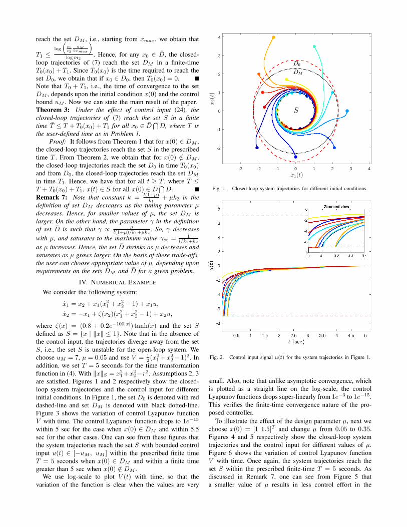
To illustrate the effect of the design parameter µ, next we

choose x(0) = [1 1.5]T and change µ from 0.05 to 0.35.

Figures 4 and 5 respectively show the closed-loop system

trajectories and the control input for different values of µ.

Figure 6 shows the variation of control Lyapunov function

V with time. Once again, the system trajectories reach the

set S within the prescribed finite-time T = 5 seconds. As

discussed in Remark 7, one can see from Figure 5 that

a smaller value of µ results in less control effort in the

0.5 1 1.5 2 2.5 3 3.5 4 4.5 5

10-15

10-10

10-5

100

Fig. 3. The evolution of the control Lyapunov function V (t) with timefor the system trajectories in Figure 1.

-1.5 -1 -0.5 0 0.5 1 1.5 2

-1

-0.5

0

0.5

1

1.5

Fig. 4. Closed-loop system trajectories for different values of µ ∈[0.05, 0.35] (blue to red).

beginning. Also, from (18), it is evident that smaller value

of µ would lead to a slower convergence-rate, which is also

clear from Figure 4.

V. CONCLUSIONS

We presented a method of designing control law for a

class of control-affine systems with input constraints so that

the closed-loop trajectories reach a given set in a prescribed

time. We showed that the set of initial conditions DM from

which this convergence is guaranteed, is a function of the

convergence time, and that this set grows larger as the input

bound or the time of convergence increases. Furthermore, the

proposed controller drives the system trajectories to this set

0.5 1 1.5 2 2.5 3 3.5 4 4.5 5

-8

-6

-4

-2

0

2

4

6

8

0 0.05 0.1 0.15-8

-6

-4

-2

0Zoomed view

Fig. 5. Control input signal u(t) for the system trajectories in Figure 4.

0.5 1 1.5 2 2.5 3 3.5 4 4.5 5

10-30

10-20

10-10

100

Fig. 6. The evolution of the control Lyapunov function V (t) with timefor the system trajectories in Figure 4.

within a finite time, that depends upon the initial condition.

Finally, we introduced a new set of sufficient conditions to

ensure the existence of a prescribed-time stabilizing con-

troller.

REFERENCES

[1] K. P. Tee, S. S. Ge, and E. H. Tay, “Barrier lyapunov functions for thecontrol of output-constrained nonlinear systems,” Automatica, vol. 45,no. 4, pp. 918–927, 2009.

[2] A. D. Ames, X. Xu, J. W. Grizzle, and P. Tabuada, “Control barrierfunction based quadratic programs for safety critical systems,” IEEE

Transactions on Automatic Control, vol. 62, no. 8, pp. 3861–3876,2017.

[3] A. D. Ames, J. W. Grizzle, and P. Tabuada, “Control barrier functionbased quadratic programs with application to adaptive cruise control,”in Conference on Decision and Control. IEEE, 2014, pp. 6271–6278.

[4] A. J. Barry, A. Majumdar, and R. Tedrake, “Safety verification ofreactive controllers for uav flight in cluttered environments usingbarrier certificates,” in International Conference on Robotics and

Automation. IEEE, 2012, pp. 484–490.

[5] S. P. Bhat and D. S. Bernstein, “Finite-time stability of continuousautonomous systems,” SICON, vol. 38, no. 3, pp. 751–766, 2000.

[6] A. Polyakov, “Nonlinear feedback design for fixed-time stabilizationof linear control systems,” IEEE Transactions on Automatic Control,vol. 57, no. 8, p. 2106, 2012.

[7] Z. Kan, T. Yucelen, E. Doucette, and E. Pasiliao, “A finite-time con-sensus framework over time-varying graph topologies with temporalconstraints,” Journal of Dynamic Systems, Measurement, and Control,vol. 139, no. 7, p. 071012, 2017.

[8] R. Aldana-Lopez, D. Gomez-Gutierrez, E. Jimenez-Rodrıguez,J. Sanchez-Torres, and M. Defoort, “On the design of new classesof predefined-time stable systems: A time-scaling approach,” arXiv

preprint arXiv:1901.02782, 2019.

[9] J. C. Holloway and M. Krstic, “Prescribed-time observers for linearsystems in observer canonical form,” IEEE Transactions on Automatic

Control, 2019.

[10] T. Yucelen, , Z. Kan, and E. Pasiliao, “Finite-time cooperative engage-ment,” IEEE Transactions on Automatic Control, (to appear).

[11] E. Arabi, T. Yucelen, and J. R. Singler, “Further results on finite-timedistributed control of multiagent systems with time transformation,”in ASME Dynamic Systems and Control Conference, 2018.

[12] ——, “Robustness of finite-time distributed control algorithm withtime transformation,” in American Control Conference, 2019.

[13] E. Arabi and T. Yucelen, “Control of uncertain multiagent systems withspatiotemporal constraints,” in American Control Conference, 2019.

[14] Y. Song, Y. Wang, J. Holloway, and M. Krstic, “Time-varying feedbackfor regulation of normal-form nonlinear systems in prescribed finitetime,” Automatica, vol. 83, pp. 243–251, 2017.

[15] Y. Li and R. G. Sanfelice, “Finite time stability of sets for hybriddynamical systems,” Automatica, vol. 100, pp. 200–211, 2019.

[16] A. Li, L. Wang, P. Pierpaoli, and M. Egerstedt, “Formally correct com-position of coordinated behaviors using control barrier certificates,” in2018 IEEE/RSJ International Conference on Intelligent Robots and

Systems. IEEE, 2018, pp. 3723–3729.

[17] P. Benner, R. Findeisen, D. Flockerzi, U. Reichl, K. Sundmacher,and P. Benner, Large-scale networks in engineering and life sciences.Springer, 2014.

[18] E. D. Sontag, “A” universal” construction of artstein’s theorem onnonlinear stabilization.” Systems & control letters, vol. 13, no. 2, pp.117–123, 1989.

[19] H. K. Khalil and J. Grizzle, Nonlinear systems. Prentice hall UpperSaddle River, NJ, 2002, vol. 3.

[20] Z. Jiang, Y. Lin, and Y. Wang, “Stabilization of nonlinear time-varyingsystems: A control lyapunov function approach,” Journal of Systems

Science and Complexity, vol. 22, no. 4, p. 683, 2009.

[21] A. D. Ames, K. Galloway, K. Sreenath, and J. W. Grizzle, “Rapidlyexponentially stabilizing control lyapunov functions and hybrid zerodynamics,” IEEE Transactions on Automatic Control, vol. 59, no. 4,pp. 876–891, 2014.

[22] M. Z. Romdlony and B. Jayawardhana, “Stabilization with guaranteedsafety using control lyapunov–barrier function,” Automatica, vol. 66,pp. 39–47, 2016.

[23] M. Jankovic, “Control lyapunov-razumikhin functions and robuststabilization of time delay systems,” IEEE Transactions on Automatic

Control, vol. 46, no. 7, pp. 1048–1060, 2001.

[24] P. Pepe, “On sontags formula for the input-to-state practical stabiliza-tion of retarded control-affine systems,” Systems & Control Letters,vol. 62, no. 11, pp. 1018–1025, 2013.

[25] Y. Shen and X. Xia, “Semi-global finite-time observers for nonlinearsystems,” Automatica, vol. 44, no. 12, pp. 3152–3156, 2008.

APPENDIX I

PROOF OF LEMMA 2

Proof: It follows from (18) and (20) that

V ′(xs) ≤ −cµ‖xs‖2S ≤ −µc

c2V (xs), (29)

where (12) and (21b) are used in the last inequality. Per

Comparison lemma, the function V (xs(s)) satisfies

V ≤ V0e−µ c

c2s, (30)

with V0 = V (xs(0)). Using (21) and (30) in (12) yields

‖xs‖S ≤ m1e−m2s. (31)

with m1 =√

V0

c1and m2 = µc

2c2> 0. Now, using (15) for

the case when b0 6= 0, the control input (16) can be rewritten

as

u = −a0b0

− µ|b0|b0

√

( a0b0θ′(s)

)2

+( b0θ′(s)

)2

, (32)

The control input upper bound can be written as

|u| ≤ |a0||b0|

(

1 +µ

θ′(s)

)

+ µ|b0|θ′(s)

(19)

≤(

l(θ′(s) + µ)

k1+ µk2

)‖xs‖Sθ′(s)

.

For the considered candidate time transformation function in

(4), one can further obtain

|u| ≤(

l(1 + µ)

k1+ µk2

)‖xs‖Se−s/T

(12)

≤ k√c1

√V

e−s/T, (33)

where k =( l(1+µ)

k1+ µk2

)

. Using (29), we obtain

|u| ≤ k√c1

√

V0e−µ c

2c2s+s/T . (34)

Hence, for T > 2c2µc , we obtain that lims→∞ |u| = 0.

APPENDIX II

PROOF OF LEMMA 3

Proof: It is clear from (24) that |u(t)| ≤ uM for all

t ≥ 0. From (34), we know that for any ǫ > 0, there exists a

δ > 0 such that if ‖x‖S < δ, then |u| < ǫ , m3δm4 . Also,

for δ <(

uM

m3

)1

m4, we know that |u| < uM , which implies

that V ′(x) < 0. So, u satisfies the small-gain property [18]

and hence, it is continuous at the origin. Since functions a, bare continuous and due to (2), |b| > 0 for ‖x‖S > 0, we

have that u is continuous for all x.

Now, assume that x(0) /∈ D0 and t = T0 is the instant

when the trajectories of (7) enter the set D0, i.e., x(T0) ∈bd(D0) and x(t) /∈ D0 for all t < T0. Then, control input at

time instant T−0 is given by

u(T−0 ) = uM

u(1, x(T0))

|u(1, x(T0))|= u(1, x(T0)),

since x(T0) ∈ bd(D0) implies |u| = uM . At time instant

T+0 , we have u(T+

0 ) = u(1, x(T0)). This implies u(T−0 ) =

u(T+0 ). Now, let t = TM be the time instant when the

trajectories of (7) reach the set DM . From (24), we know

that

u(T+M ) = u(θ′(θ−1(t− TM )), x(t))|t=TM

= u(θ′(θ−1(0)), x(TM ))(3)= u(1, x(TM )) = u(T−

M ),

which completes the proof.