KRANNERT SCHOOL OF MANAGEMENT · Krannert School of Management Purdue ... Buyers then decide...

KRANNERT SCHOOL OF MANAGEMENT Purdue University West Lafayette, Indiana

Costly Buyer Search in Laboratory Markets with Seller

Advertising

By

Timothy N. Cason Shakun Datta

Paper No. 1212 Date: April, 2008

Institute for Research in the Behavioral, Economic, and Management Sciences

Costly Buyer Search in Laboratory Markets with Seller Advertising*

Timothy N. Cason Department of Economics

Krannert School of Management Purdue University

West Lafayette, IN 47907

and

Shakun Datta Department of Economics Robins School of Business

University of Richmond Richmond, VA 23238

April 2008

Abstract In this laboratory experiment sellers simultaneously post prices and choose whether to advertise. Buyers then decide whether to buy from a seller whose advertisement they have received, or engage in costly sequential search to obtain price quotes from other sellers. In the unique symmetric equilibrium, sellers either charge a high unadvertised price or randomize in an interval of lower advertised prices. Increases in either search or advertising costs raise equilibrium prices, and equilibrium advertising intensity decreases with lower search costs and higher advertising costs. Our results are consistent with most of these comparative static predictions, and sellers also post lower advertised than unadvertised prices as predicted. In all treatments, however, sellers price much lower than the equilibrium interval and earn very low profits. Although buyers’ search decisions are approximately optimal, sellers advertise more intensely than predicted. Consequently, market outcomes more closely resemble a perfect information, Bertrand-like equilibrium than the imperfect information, mixed strategy equilibrium that features significant seller market power.

JEL Classification: D43; D83; L13 Keywords: Experiment; Posted offer; Market power; Mixed strategy; Uncertainty; Shopping

*We thank Jacques Robert, Emmanuel Dechenaux, David Reiley, Andrew Yates, the editor, and two anonymous referees for helpful suggestions, Jeff Bayer for research assistance, and seminar audiences at Harvard and Michigan State Universities, the Universities of Amsterdam, Arizona, Nottingham and Tilburg, and the Wissenschaftszentrum Berlin (WZB) for useful feedback. The Purdue University Faculty Scholar program and the Purdue Research Foundation provided financial support.

1. Introduction

If buyers are perfectly informed about seller prices of a homogeneous product, then the

outcome of Bertrand competition is marginal-cost pricing. Imperfect information about seller

prices, however, can lead to market power. At the extreme, if buyers must search for prices

sequentially with strictly positive search costs, then in equilibrium no buyer would search and all

sellers would charge the monopoly price (Diamond, 1971). But as Robert and Stahl (1993)

emphasize, sellers have an incentive to advertise lower prices, thereby undermining the

monopoly equilibrium. They introduce advertising in a sequential costly buyer search model,

where the differentially-informed buyers yield a market equilibrium that is characterized by price

dispersion. This price variance gives buyers the incentive to search for lower prices. Non-

dispersed price equilibria do not exist because of a cyclical best response structure for the sellers:

the best response to a rival charging some price p is to charge a price fractionally below p (as in

Bertrand competition), but unlike perfect information models there typically exists some lowest

price p for which the best response is not undercutting but is instead charging a high

unadvertised price and selling only to uninformed buyers.

The “law of one price” is not an empirical regularity; in fact, even Stigler (1961, pg. 213)

observed that “dispersion [of prices] is ubiquitous even for homogenous goods.” Economists’

interest in price dispersion has been renewed recently based in part on field evidence that it

persists even as information technologies have reduced search costs. For example, Brynjolfsson

and Smith (2000) document substantial price dispersion on Internet price comparison sites, and

Baye, Morgan and Scholten (2004) find large and persistent price dispersion in what appears to

be essentially homogenous goods markets. But one limitation of the field evidence is that it

rarely can include truly homogeneous products as typically assumed in theory. Even when the

items being purchased are identical products produced by the same manufacturer (as Baye et al.

consider), the retail distribution typically features differences in customer service, reputations,

and (particularly relevant for Internet retailing) beliefs in delivery reliability. The observed price

dispersion in the field data might therefore reflect some of these unobserved differences between

sellers of an identical product. Laboratory methods provide alternative empirical evidence by

controlling and manipulating these variables that are difficult to measure in the field.

In this paper we examine laboratory markets that are broadly consistent with assumptions

typically made in competitive models of costly buyer search and informative price advertising.

2

The experiment is specifically structured by Robert and Stahl’s stylized model in which buyers’

information is endogenously determined along with seller prices, advertising and profitability.

Sellers are not capacity constrained, and buyers demand at most one unit per trading period. In

the unique symmetric Bayesian equilibrium, sellers either charge a high unadvertised price or

randomize in an interval of lower advertised prices, and buyers conduct at most one search per

period. Increases in either search or advertising costs raise equilibrium prices, and equilibrium

advertising intensity decreases with lower search costs and higher advertising costs. Our results

are consistent with the pattern from previous posted-price market experiments in that behavior

deviates from the quantitative theoretical predictions, but broadly conforms to the equilibrium

comparative statics (Brown-Kruse et al., 1994, Morgan et al. 2006a,b). Sellers in our experiment

also post lower advertised than unadvertised prices, as predicted. In all treatments, however,

prices are significantly lower than the equilibrium price interval and sellers earn profits that are a

fraction (12 to 40 percent) of the equilibrium level. Prices are also not as dispersed as predicted

by theory. Buyers’ search decisions, although approximately optimal, exhibit a small bias

towards under-searching. Sellers advertise more intensely than in equilibrium, which results in

widespread diffusion of information. Consequently, market outcomes more closely resemble a

perfect information, Bertrand-like equilibrium than the imperfect information, mixed strategy

equilibrium that features significant seller market power.

These results with human buyers contrast sharply with our previous study (Cason and

Datta, 2006), which reports sessions with robot buyers that are pre-programmed to search

according to an observable equilibrium reservation price strategy. Those sessions with robot

buyers provide almost uniformly positive support for the theoretical model. The data support all

of the model’s comparative static predictions; and similar to this study, the only systematic

deviation from the quantitative predictions is that observed advertising rates exceed the predicted

rates. The crucial difference is that unlike this study, the observed price levels in robot buyer

sessions are broadly consistent with the predicted equilibrium price levels. A comparison

between these two studies indicates that a fundamental difference exists in the behavioral

equilibrium when the robot buyers’ reservation price search strategies are replaced with human

buyers. The robot buyers’ expectations and behavior is unaffected by observation of non-

equilibrium prices, while human buyers’ expectations can adjust to low seller prices. Seller

advertising pushes prices to still lower levels, away from equilibrium, and buyers observe more

3

than one price before purchase 2 to 6 times more frequently than the rate expected by the

equilibrium analysis.

We return later to the contrast between sessions with human and robot buyers, and only

point out here that such dramatic differences in outcomes are not anticipated by earlier research

that does not feature seller advertising. For example, Cason and Friedman (2003) and Davis and

Williams (1991) employ both robot and human buyers in different posted offer market

treatments. These earlier experiments indicate more variable market outcomes in the human

buyer sessions than in the robot buyer sessions, but the equilibrium predictions were generally

supported even with human buyers.

The remainder of the paper is organized as follows. Section 2 presents Robert and Stahl’s

(1993) model of costly advertising and search, simplified to the experimental conditions and

parameters chosen for our laboratory implementation. It also summarizes the model’s

comparative statics and hypotheses for the experiment, based on formal propositions and proofs

drawn from Cason and Datta (2006). Section 3 provides details of the experimental design and

procedures, and Section 4 contains the empirical results and discussion. Section 5 concludes.

2. Theoretical Model

Consider a market where n identical sellers compete to supply a homogenous product to a

fixed number of buyers who have an identical valuation v for one unit of the good. Each seller

produces at a constant marginal cost, which is normalized to zero, and has no fixed costs or

capacity constraints. The sellers can inform the buyers about their price through advertising at a

cost A. If sellers choose to advertise, they reach a fixed proportion α of the buyers.1

Buyers are a priori uninformed about the prices in the market but can obtain this

information either through receiving an advertisement from sellers or by conducting search at a

cost c per price quote. This search is without replacement and with perfect recall. Each buyer has

an independent probability of being informed of seller j’s price. The ads are randomly distributed

across buyers; i.e., sellers cannot target their advertising nor can the buyers influence the

probability of receiving an advertisement.

At the beginning of each period, all sellers choose simultaneously their price and make

1 This is a simplifying assumption. In the original Robert and Stahl model, sellers also choose their advertising intensity; i.e., the proportion of buyers that they wish to reach. Making the advertising intensity decision exogenous, however, has no impact on the qualitative results.

4

their binary advertising decision—whether or not to advertise this price. After advertised prices

are conveyed to (some of the) buyers, buyers make their search decisions. Buyers who receive no

ad must search to receive their first price quote. Buyers who receive an ad can choose to buy

from a seller whose ad they have received or conduct costly sequential search to obtain

additional price quotes from other sellers.

Optimal buyer search endogenously determines a unique reservation price, r, which equates

the marginal benefits of search to the cost of search, c. According to the reservation price

strategy, buyers will continue search until they find a price that is less than or equal to r. Further,

each buyer buys one unit of the good from the seller offering the lowest advertised price, pj, only

if pj + c ≤ min{r, v}.2, 3

In the unique symmetric perfect Bayesian equilibrium the sellers randomize between

advertising and not advertising. The (mixed) price strategy is given by the price distribution F(.)

with support contained in (0, v). More specifically, the support of the distribution is the union of

the interval [pl, r-c] and the reservation price {r}, where pl is the lower bound of the equilibrium

distribution.4 Since buyers will never purchase at a price greater than their reservation price, r is

the maximum price that the sellers will ever charge. Moreover, the distribution has a mass point

at r since the sellers will never charge a price between r and r-c.5 Finally, there is no mass point

in the distribution at or below r-c since it is always profitable to break a potential tie by

marginally decreasing the advertised price.

The specific functional form of the equilibrium seller advertising and pricing strategy is

summarized in the following proposition (for formal proof see Cason and Datta, 2006).

Proposition 1: Given search cost c>0, advertising intensity α>0 and n≥2 sellers, if the

advertising cost A is strictly less than ( )( 1)v c nn

α− − , there exists a unique symmetric mixed

strategy equilibrium such that:

Sellers advertise ( , )lp p r c∈ − but do not advertise p = r; and set price according to the

2 This follows from the fact that a buyer who decides to buy at the advertised price will still have to incur a one-time transportation cost of c to procure the good from the seller. 3 This reservation price rule holds only if there is at least one unknown price. In the case where buyers receive prices ads from all sellers, they purchase at the lowest advertised prices pj, as long as pj + c ≤ v. 4 Since advertising intensity is exogenously fixed at α>0, the equilibrium outcome does not converge to Bertrand equilibrium as information costs go to zero. 5 The choice of a price less than r is justified only if the seller decides to advertise the price, but given the buyer’s search/transportation cost c to purchase at the advertised price, this price must be at most r-c.

5

following distribution function:

( )( )

11α 1 ( ) (1 )1

α α α 1 ( )( ) 1 if [ , ]

( ) if ( , )1 if

nA n r c plp n r c rF p p p r c

F r c p r c rp r

α α

α

−+ − − − −⎡ ⎤⎣ ⎦+ − − −⎡ ⎤⎣ ⎦

⎧ ⎡ ⎤⎡ ⎤≡ − ∈ −⎪ ⎢ ⎥⎣ ⎦⎪ ⎣ ⎦⎨

− ∈ −⎪⎪ ≥⎩

where the lower bound of the distribution is given by ( )( )( )

α 1 ( )α α 1 ( ) (1 )

A n r cl n r c r Ap α

α α+ − −

+ − − − + −= ;

and the (maximum) buyers’ reservation price, r, is implicitly given by [ ]

(1 ) ( )

1 ( )l

r c

p

F p dpc

F r c

α−

−

=− −

∫.

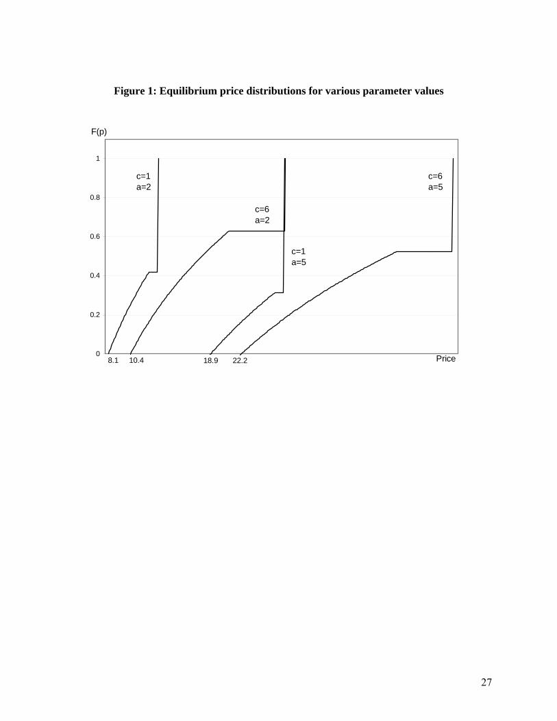
Figure 1 illustrates the equilibrium price distributions for parameter values used in the

experiment. It also provides a graphical presentation of the comparative statics regarding search

and advertising costs. Formal statements of the comparative statics and other technical details are

contained in Proposition 2 and 3 of Cason and Datta (2006) but the rationale underlying each

comparative static prediction is detailed in the hypothesis below.

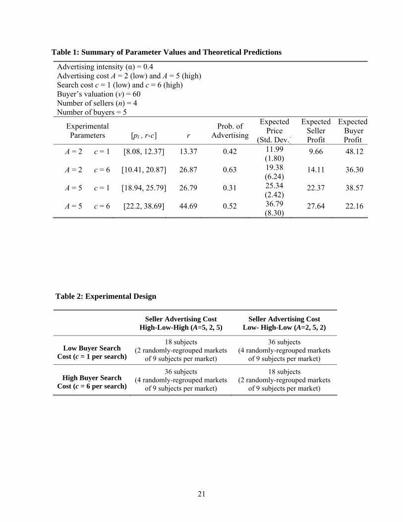
Table 1 summarizes the parameter values used in the experiment and the theoretical

predictions for the various treatments. The expected price refers to the overall weighted average

of posted prices, including both advertised and unadvertised prices. Since strong quantitative

predictions such as those shown in Table 1 rarely hold precisely in experimental studies, our

empirical analysis will focus on the weaker, comparative static predictions summarized by the

following hypotheses. The first three hypotheses concern the sellers’ equilibrium pricing and

advertising behavior in response to varying levels of search and advertising cost. The last two

hypotheses concern buyer search behavior.

Hypothesis 1a: An increase in search cost results in higher prices.

Hypothesis 1b: An increase in search cost results in increased incentives for the sellers to

advertise, and higher seller profits.

As search cost increases, buyer search propensity decreases. This decline in buyer search has two

effects. One, it gives the sellers more market power, resulting in higher prices. Two, it creates an

incentive for the sellers to inform the buyers through advertising. Since the benefit of higher

prices may be offset by increased advertising expenditures, the impact of search cost on seller

profit would appear to be ambiguous. However, for a wide range of parameters the price effect

6

dominates the increased advertising expenditure effect so that profit increases as c increases.

Hypothesis 2a: An increase in advertising cost results in higher prices.

Hypothesis 2b: An increase in advertising cost reduces the sellers’ propensity to advertise

and results in higher profits.

The direct effect of an increase in advertising cost is to reduce the seller’s incentive to advertise.

The indirect effect of an increase in advertising cost is a shift in the cumulative price distribution

so that sellers place a greater weight on higher prices. Higher prices combined with lower

propensity to advertise result in increased profits.

Hypothesis 3: Unadvertised prices are higher than advertised prices.

This follows directly from the characterization of the equilibrium: sellers either charge a high

unadvertised price or randomize in the interval of lower advertised prices. The reservation price r

is the maximum price charged by a seller. Advertising this price will not induce the informed

buyers to visit the seller to make a purchase, since the effective purchase price becomes r+c.

Conversely, a seller will choose a price below r-c only if she advertises it.

Hypothesis 4: Controlling for observed prices and beliefs, buyers search more frequently

when search costs are lower.

In the present model, a lower cost of search implicitly yields a lower reservation price r.

Therefore, the likelihood that any given price distribution includes prices greater than r is higher

when the search cost is low. Accordingly, buyers are more likely to search in case of low search

cost. Laboratory studies by Schotter and Braunstein (1981) and Cason and Friedman (2003) have

also documented the monotonic relationship between cost of search and propensity to search.

Hypothesis 5: Buyers search according to an optimal search rule.

The perfect Bayesian Nash equilibrium is characterized by “no real search.” That is, in

equilibrium, sellers do not price above the reservation price r and therefore, buyers do not find it

optimal to search more than one seller. This result, however, is based on a number a strong

assumptions that may not hold in practice. Differing experience is likely to encourage differing

beliefs and behavior, which may delay or even prevent convergence to equilibrium. In particular,

7

buyers in the experiment may hold imprecise beliefs because they face an endogenous price

distribution that is both unknown and unstable. Sellers’ pricing and advertising strategies may in

turn be responsive to the (possibly non-equilibrium) buyer search strategy.

Therefore, while it is plausible that human buyers follow some search rule, they may not

strictly follow a reservation price strategy, much less an identical and unchanging reservation

price strategy as called for in the equilibrium. Accordingly, the assessment of the optimality of

some particular search behavior should account for the actual price draws the buyer can receive,

and additional search should be regarded as optimal if the expected price reduction exceeds the

cost of search. Our analysis compares the buyers’ search decisions to an optimal search rule that

is based on an “empirical” reservation price which changes over time in response to the history

of seller price offers.6

3. Experimental Design and Procedures

3.1 Experimental Design

Each market comprises 4 sellers and 5 buyers. The trading institution modifies the standard

posted-offer environment by incorporating two treatment variables – seller advertising and buyer

search. Sellers can reach a fixed proportion α = 0.4 of the buyers (that is, 2 of the 5 buyers) by

incurring an advertising cost A. Buyers can obtain price quotes from sellers by engaging in

search at a cost c per quote. The experimental design is summarized in Table 2.

We vary advertising costs within sessions and search costs across sessions. In six of the

markets, referred to as “High-Low-High,” sellers face a high advertising cost (A = 5) in the first

25 periods, low advertising cost (A = 2) in the next 25 periods and high advertising cost again in

the last 25 periods. The order is reversed for the six “Low-High-Low” markets. The two levels of

buyer search cost used in the experiment are c =1 and c = 6. The data identify the effect of a

change in search cost by making the relevant across-sessions comparisons while within-session

comparisons assess the effect of change in advertising cost.

To minimize repeated game effects and reduce the incentives for collusive behavior, we 6 This is only an approximation since buyers’ beliefs are not observed directly. Moreover, since our design limits the number of sellers in each market, consistent with the finite horizon search literature, the reservation price should be increasing in the number of searches. In a labor market context with a search environment similar to ours, both the theoretical (e.g. Gronau, 1971, and Lippman and McCall, 1976) and the experimental literature (e.g. Schotter and Braunstein, 1981, and Cox and Oaxaca, 1989) have concluded that “the introduction of a finite horizon leads to abandonment of the constant reservation wage property …[although] the qualitative implications of the model for changes in variables such as the direct costs of search are unchanged” (Cox and Oaxaca, 1989, pg. 306).

8

randomly re-match subjects each period. We made this design choice because we are testing a

static model. The drawback of this design feature is that only the six pairs of the 12 markets are

statistically independent; however, the data analysis accounts for the correlation of repeated

observations contributed by individual subjects through random effects error specifications.

3.2 Experimental Procedures

The experiment consisted of six 2-hour sessions, each containing 18 subjects, all conducted

in the Vernon Smith Experimental Economics Laboratory at Purdue University. A computerized

interface using the software z-Tree was used to implement the experiment (Fischbacher, 2007).

The subjects were recruited from undergraduate economics classes, and all were inexperienced

in the sense that no one participated in more than one session of this type. Upon arrival, the

subjects were seated at separate, visually isolated computer terminals and no communication was

permitted throughout the session. Each subject received a set of instructions and record sheets,

included as a supplementary materials Appendix on the journal web page. The instructions were

read aloud, so we assume that the information contained in them was common knowledge.

Each session proceeded through a sequence of 75 trading periods. All sellers had the same

homogenous good whose cost of production was normalized to zero. The sellers did not face any

capacity constraint. Each buyer demanded at most one unit, and received a resale value of 60

experimental francs if they purchased this unit. At the start of a trading period, each seller posted

a single price offer and chose whether to advertise this price. After all sellers made their pricing

and advertising decision, some of the buyers received a price advertisement. Each advertising

seller’s price was equally likely to be shown to each buyer and the advertisements were

distributed randomly. Note that some buyers could receive multiple ads while others in the same

market might not receive any ads. Buyers then made their search and purchase decisions. The

buyers who received advertisement(s) decided whether to search for other prices or to buy a unit

at an advertised price. If a buyer decided to search other sellers, he had to pay the transportation

cost for each different price quote. If he decided to buy at the advertised price, he had to pay a

one-time transportation cost to obtain the good from the seller. All transactions, costs and

earnings were in experimental francs, which were converted to U.S. dollars at the end of the

experiment using a known but private dollar conversion rate. The earnings typically ranged

between $15 and $40 per subject, with an average of $25.50.

9

At the end of each period, each seller was informed about the number of units he or she

sold, and each buyer and seller received a summary of their own current period and cumulative

earnings. Following Cason and Friedman (2003) and Morgan, Orzen and Sefton (2006b), at the

end of each period in four of the six sessions all buyers and sellers also learned the prices,

quantities sold and advertising decisions of all sellers in their market. These prices were

displayed from the lowest to the highest and did not reveal the identities of the individual

sellers.7 In the analysis we code these four sessions as full information sessions, and the other

two sessions (which reported only the subjects’ private outcomes) as partial information

sessions. The difference in information feedback led to only minor differences in results.

4. Experimental Results

We divide the results into five subsections. Section 4.1 presents an overview of the price

and advertising data to orient the reader. Section 4.2 provides analysis of seller pricing and

advertising behavior and section 4.3 analyses buyer search and purchase behavior. Section 4.4

calculates the seller best-responses given the buyer search behavior and other sellers’ choices,

and in Section 4.5 we discuss possible explanations for the observed disequilibrium behavior.

4.1 Overview of Posted Prices

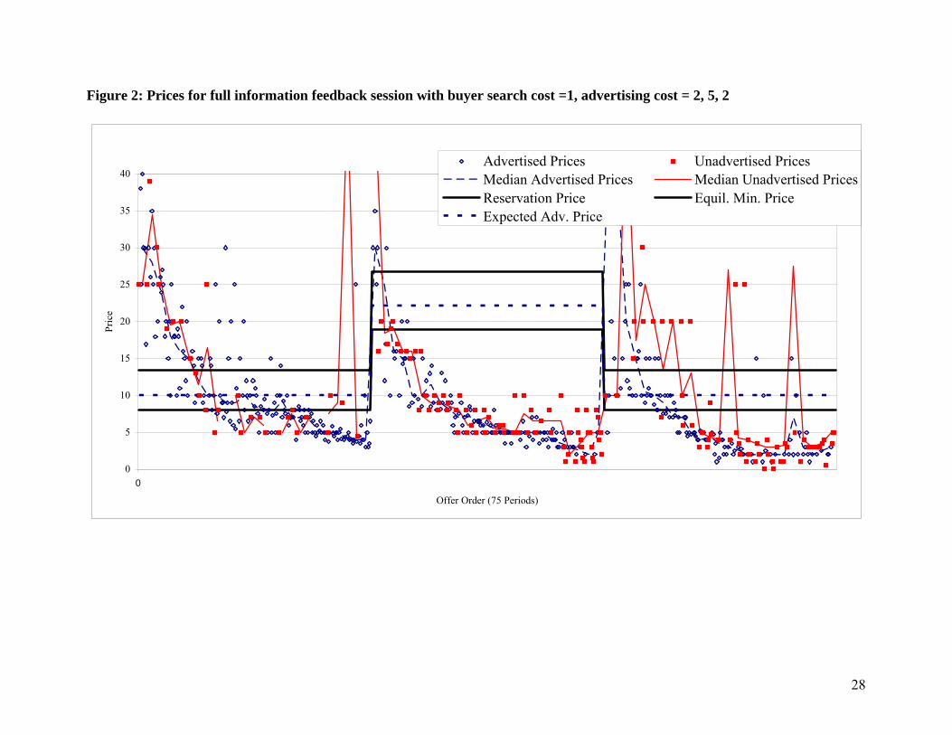
Figures 2 and 3 summarize the prices and present the most striking departures from the

equilibrium model that we are aware of, in the experimental literature on market with incomplete

information. Figure 2 report all individual prices in all 75 periods in one of the six sessions.

Open circles denote advertised prices and closed squares denote unadvertised prices. The

connected dashed and solid lines display median advertised and unadvertised prices, and the

horizontal lines indicate equilibrium price predictions. The equilibrium predictions shift in

periods 26 and 51 because we switched advertising cost every 25 periods.

Prices tend to begin above, within or below the equilibrium range for the first few trading

periods. Without exception, however, sellers eventually post very low prices. Only the treatment

7 Abrams, Sefton and Yavas (2000) did not reveal to the seller the prices posted by other sellers in the market. They found that prices, even in the later periods, deviated significantly from the predicted level. Cason and Friedman (2003) on the other hand, found a much stronger support for the theoretical prediction and part of this difference in the results may be explained by difference in the information feedback to the sellers. Offerman, Potters and Sonnemans (2002) manipulate the feedback in a quantity-setting oligopoly experiment without search or advertising, and find that outcomes vary with the feedback in directions predicted by models of behavioral dynamics.

10

switchovers that occur every 25 trading periods reliably interrupt the downward price trends,

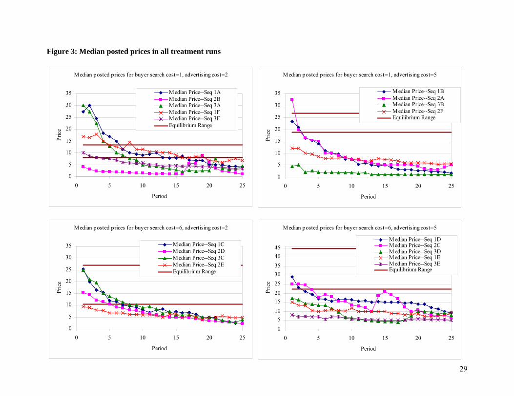
although in some sessions sellers are able to increase prices within a treatment run. Figure 3

shows the median posted prices for all sessions, with different treatments separated in different

panels. It clearly indicates that downward price pressure is a robust, dominant feature of our data.

Sellers ultimately post prices that are almost entirely below the lower endpoint of the equilibrium

price interval in all sessions and all treatments. Median prices typically fall below 5 francs,

except in the lower-right treatment that features the highest advertising and search costs.

Figure 2 also provides an initial impression of the “over-advertising” that we document

formally in the next subsection. The open circles vastly outnumber the closed squares, indicating

that sellers more often choose to advertise their prices.

4.2 Seller Advertising and Pricing Behavior

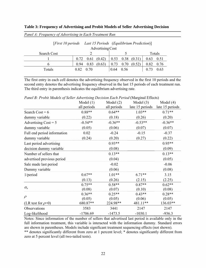
Seller Advertising Behavior. Panel A of Table 3 presents the observed frequency of advertising

in the first 10 as well as the last 15 periods of each treatment run for different search cost-

advertising cost combinations. A comparison to the theoretical prediction reveals that the

observed advertising rate always exceeds the model’s prediction. Equilibrium advertising rates

range between 0.31 and 0.63 across the four treatments, while the actual advertising rates

average between 0.53 and 0.94 when calculated over the first 10 periods of each treatment run.

The frequency of advertising declines in later periods, but still remains well above predicted

levels in all treatments. While aggressive advertising behavior is a prominent feature of the data,

note that the ordering of the advertising propensity across various treatments is nevertheless

consistent with the comparative statics predictions of the model. Advertising rates always

increase with higher buyer search costs and decrease with higher advertising costs.

In order to assess the statistical significance of these results we use panel data econometric

models with a subject level random effects error specification. Panel B of Table 3 reports the

results of probit models for the seller advertising decision. The models include 1/period to

control for time trend. Since the time trend is more pronounced in the early periods of each run,

we present estimates based on all 25 periods in Models 1 and 2, as well as based on the last 15

periods of each treatment run in Models 3 and 4.8

8 We also examined a variety of alternative model specifications. For example, we added an interaction term for the high search cost and high advertising cost dummy variables to allow for different advertising rates in each of the

11

Result 1: An increase in advertising cost reduces the sellers’ propensity to advertise

(Hypothesis 2b).

Support: Panel A of Table 3 indicates that in both search cost treatments, the advertising rate is

always lower with higher advertising costs (0.38 to 0.70) than with lower advertising costs (0.61

to 0.83). The probit models shown in Panel B indicate that this impact of advertising cost on

seller advertising is significant at one-percent level in all specifications and for both all periods

and late periods data.

Result 2: An increase in search cost increases the sellers’ propensity to advertise

(Hypothesis 1b).

Support: As search cost increases, buyer search intensity decreases. This raises incentives for the

sellers to inform the buyers about their prices. Panel A of Table 3 provides strong support for this

prediction. For instance, when A =5, as search cost increases from c=1 to c=6 the late periods’

frequency of advertising almost doubles from 0.38 to 0.70. The regressions in Panel B provide

statistical evidence that rejects the null hypothesis of no search cost treatment effect at any

conventional level of significance, for different model and period specifications. In fact, a

comparison of the advertising cost and the search cost coefficient estimates suggests that the

indirect effect of search cost on seller advertising propensity is at least as important as the direct

effect of advertising cost.

Note that although the advertising rate generally exceeds the model’s prediction, the

positive coefficient estimate on 1/period indicates that the frequency of advertising tends to

decrease over time. This decline in advertising propensity may be related to the decline in prices,

which is documented next.

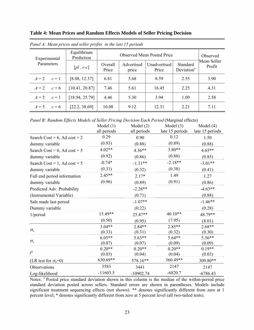
Seller Pricing Behavior. Panel A of Table 4 summarizes mean posted prices in the last 15 periods

for different cost treatments. Observed prices are always too low compared to the theoretical

expected price, and they are too low even compared to the theoretical minimum price. The over-

four treatments. This interaction term was always statistically insignificant and including it does not change any of the general conclusions we draw in the reported analysis.

12

advertising documented above results in a more transparent pricing environment, which appears

to lead sellers to price more aggressively than predicted in equilibrium.

Result 3: An increase in advertising cost leads to higher prices, but only in the presence of

high buyer search costs (Hypothesis 2a).

Support: Panel A of Table 4 shows that as advertising cost increases from A=2 to A=5, the mean

advertised price increases substantially when c=6 but it declines slightly when c=1. Similarly,

although the random effect regression models (Panel B of Table 4) reject the null hypothesis that

there is no advertising cost treatment effect, they indicate that advertising cost acts as a

“facilitating device” to raise prices only when search costs are high. Higher advertising costs

exert a smaller but statistically significant downward influence on prices when search costs are

low.

Result 4: An increase in search cost leads to higher prices, but only in the presence of high

advertising costs (Hypothesis 1a).

Support: Price averages in panel A and random effects regressions in Panel B of Table 4 indicate

that in spite of the surprisingly low prices, the data support the comparative statics for search

cost when advertising costs are high. Search costs do not significantly influence prices when

advertising costs are low, perhaps because advertising is very frequent in this case (cf Table 3).

Result 5: Unadvertised prices are higher than advertised prices

Support: Analyzing the data for each search-ad cost difference separately (Panel A of Table 4),

in all cases, except one, the average unadvertised price exceeds the average advertised price.

Random effects models which control for time trend and sequence fixed effects also provide

statistical evidence in favor the alternative hypothesis that advertised price is lower than the

unadvertised price. The current period advertising decision is obviously endogenous, so we use

an instrumental variables approach in which the actual advertising choice is replaced by the

predicted advertising probability based on the probit models reported in Table 3. The negative

advertising probability coefficients in models 2 and 4 of Table 4 indicate that advertised prices

are lower than unadvertised prices.

13

Result 6: Prices are less dispersed than predicted, except for the treatment with low search

and advertising costs.

Support: The sixth column in Panel A of Table 4 summarizes the observed posted price

dispersion. (We report the median within-period standard deviation because the mean dispersion

is sensitive to some outliers caused by occasional non-serious price offers.) Comparing the

observed dispersion to the equilibrium dispersion shown in Table 1 reveals that prices are less

dispersed than predicted in 3 out of the 4 treatments. To provide a statistical comparison with the

equilibrium dispersion, we employed a Monte Carlo simulation of 1000, 15-period price

sequence draws from the equilibrium distribution to construct a 90-percent confidence interval

for the price standard deviation for each treatment. Excluding the low search and advertising cost

(A=2, c=1) treatment where price dispersion is greatest, the observed median price standard

deviation for the later 15 periods falls below this 90-percent confidence interval in 20 of the 26

separate treatment runs.

4.3 Buyer Search Behavior

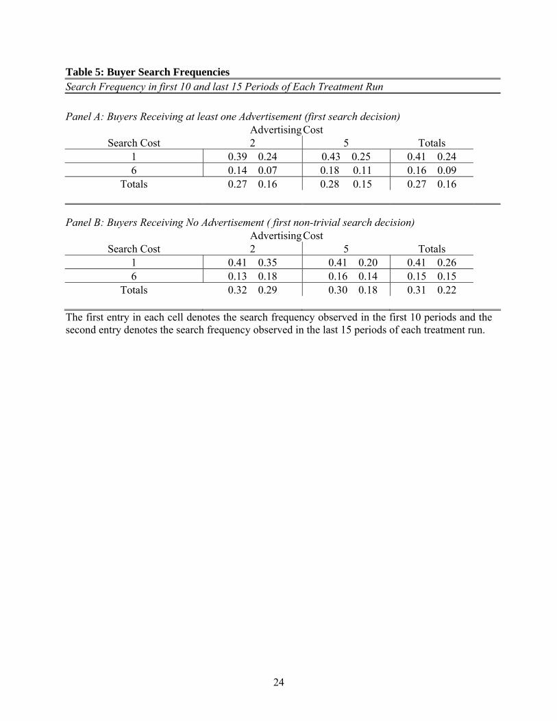
Panel A of Table 5 presents overall search rates by treatment for buyers who receive at

least one ad. These rates indicate how often buyers do not buy immediately at the advertised

price, but instead decide to search another seller. We include in this analysis only the

nondegenerate cases in which buyers have received at least one advertised price but less than all

four advertised prices. Panel B of Table 5 presents the rates of the first “non-trivial” search for

buyers who receive no ad. Recall that buyers who do not receive any ad must search to get their

first price quote, so these rates indicate how often such buyers search more than one seller.

Recall that in equilibrium, buyers search and purchase from only one seller because sellers

never post prices above buyers’ reservation price. In the experiment, nearly all the posted prices

were below the equilibrium reservation price, so according to the optimal search strategy, the

equilibrium search rate for all cells of Table 5 would be near zero. Out of equilibrium, imprecise

buyer beliefs, disequilibrium price distributions that change over time, or other factors, make

searching more attractive. Table 5 indicates that search frequency typically declines in the later

15 periods compared to the first 10 periods as prices tend to stabilize following initial adjustment

to the new treatment conditions. Comparing search rates across treatments, an increase in search

costs clearly decreases the frequency of search. For example, Panel A indicates that the search

14

frequency of ad-receiving buyers more than doubles (from 9 percent to 24 percent) in the c=6

treatment compared to the c=1 treatment in the later periods of the treatment runs. The

corresponding increase in Panel B is also high. The impact of advertising cost on buyer search

decisions is indirect in theory and has a smaller impact on observed search behavior.9

The above documentation of search behavior does not indicate whether buyers are

searching optimally. Previous experimental research has studied the simpler problem of

sequential search for a price (or wage) given a fixed and known price or wage distribution (e.g.,

Schotter and Braunstein, 1981; Cox and Oaxaca, 1989; Harrison and Morgan, 1990), and

indicates that searchers behave approximately optimally with a small bias towards stopping

search too soon.10 However, unlike this earlier research, buyers in our study face an unknown

and unstable price distribution. Moreover, evaluating the optimality of buyer search is

complicated further because the realized distribution of seller prices differs vastly from the

equilibrium distribution. Indeed, depending on the buyers’ beliefs, a reservation price strategy

may not even be optimal (Cox and Oaxaca, 2000). Nevertheless, we can still apply the logic of

an optimal stopping rule for this sequential search problem to estimate whether the buyers’

search strategy, ex post, is approximately optimal. Our analysis strategy involves a comparison

of the search behavior and expected returns from search to estimate whether buyers tend to over-

or under-search given the observed prices and advertising decisions of sellers.

First, we calculate an approximate “empirical” reservation price. Analogous to its

equilibrium counterpart, this reservation price equates the expected benefit from search to the

cost of search. The primary difference, however, is that in this case the conditional expectation of

price is computed over actual price draws that a buyer could have received upon search. To

account for the steep decline in prices typically observed in the initial periods of a treatment run,

for the first 15 periods we base this expected value on an historical three-period moving average,

followed by a fixed 10-period average during the final ten periods of the treatment run where

prices are more stable. The empirical reservation price indicates whether searching an additional

9 A series of (unreported) random effect probit regressions formally document these observations. Controlling for a variety of other factors, we find that the impact of search costs on search frequency is significant at the one-percent level in various specifications and for both the late periods and all periods data. Moreover, we find that on the whole buyers respond reasonably to the potential search benefits. Buyers search with greater frequency when the lowest price advertisement they receive is higher, and also when they only receive one advertised price, compared to when they receive two or three advertised prices. 10 Hey (1981, 1982) and Sonnemans (1998) explain this more common error of stopping search too soon by noting that expected losses from errors are asymmetric, with smaller losses from a higher-than-optimal reservation price.

15

seller is optimal or not, based on the actual price draws available to the buyers.

Second, we compare actual buyer search behavior to the (approximately) optimal search

rule. As before, we draw a distinction between a buyer who receives at least one ad and a buyer

who receives no ads. Recall that the search cost must be paid to buy from an advertising seller,

so for a buyer who receives ad(s) search is optimal if the (minimum) observed price plus the

search cost is greater than the empirical reservation price. By contrast, a buyer receives no ad

must search to receive a price quote, so the search cost becomes sunk and the decision of

whether an additional search is optimal depends simply on whether the minimum observed price

exceeds the empirical reservation price.

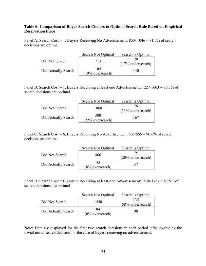
When buyers fail to search optimally, it is useful to divide their mistakes into 2 types of

errors: undersearch and oversearch.11 Table 6 presents the optimal search comparisons for the

first two search decisions made in each period.12, 13 When c=6, shown in the lower part of the

table, 85 to 90 percent of the search decisions are optimal. Errors that occur more commonly take

the form of undersearch rather than oversearch. When c=1, the proportion of optimal search

decisions is slightly lower but still quite high. Also, oversearch and undersearch rates are similar

when c=1, in contrast to the more systematic undersearch when c=6.

Overall, the observed search choices compared to an empirically-based optimal

reservation price strategy indicates that the buyer search behavior is close to optimal. Consistent

with the previous literature on sequential search, the pattern of error exhibits a bias towards

stopping too soon (undersearch), especially with high search costs.

4.4 Seller Best Responses

In this subsection we show that the low prices posted by sellers in later periods, though

far from the equilibrium predictions, are close to best-responses to the pricing and advertising

decisions of other sellers and the search decisions of buyers.

11 Type 1 error or undersearch: Buyers did not search when they should have searched i.e., buyers did not search when the observed price draw (possibly inclusive of search cost) is greater than the empirical reservation price. Type 2 error or oversearch: Buyers searched when they should not have searched i.e., buyers searched when the observed price draw (possibly inclusive of search cost) is less than the empirical reservation price. 12 The first two search decisions comprise about 95 percent of decisions made by buyers in case of low search cost. When c=6, search propensity decreases further and therefore these computations include 99.4 percent of all buyer search decisions. 13 We focus on the impact of varying levels of search cost on buyer search decision. Search costs enter buyer decisions directly, and as discussed earlier in this subsection, have a pronounced and predictable effect on search behavior. The impact of ad cost, on the other hand, is indirect since it operates through changing seller behavior.

16

To document this we calculate the sellers’ empirical best responses based on buyer search

behavior and on 1000 simulated iid draws of three rival sellers advertising and pricing strategies.

We select these draws from all sellers choices during the final 15 periods of each treatment,

where prices tended to stabilize following the initial adjustment period to a new treatment

condition. The simulation accounts for buyer search and purchase behavior by translating each

combination of four advertising and price choices into an expected sales quantity using an

ordered logit model, also estimated on these final 15 periods of each treatment. This generates a

probability of selling zero through 5 units, which in turn determines the expected profits for that

price and advertising choice.14 In other words, we estimate the expected profitability of each

possible price and advertising strategy by simulating 1000 rival seller strategies and a

probabilistic model of buyer search and purchasing strategies, all based on the late periods of

each treatment. Finally, the simulation employs a grid search over prices (at 5-cent increments)

to identify the best strategy.

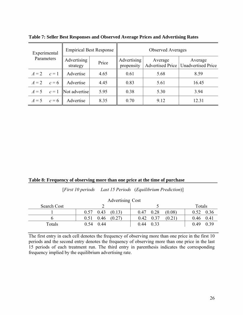
Table 7 summarizes the best-response advertising and pricing strategy for the different

treatments. In three out of the four treatments, the best strategy for the seller is to advertise and

post relatively low prices.15 It is only when A=5 and c=1 that advertising is not the best strategy

for the seller. In this treatment due to the inexpensive search cost, on average the sellers are not

able to recover enough of their advertising cost to make advertising worthwhile..

The right side of Table 7 permits a comparison of the best-response advertising and

pricing strategy with the observed seller choices. The best-response prices, ranging from 4.45 to

8.35, are not very different from the observed average prices. Furthermore, consistent with the

observed prices, the best-response prices calculated from these simulations are well below the

lower bound of the equilibrium price distribution. Observed advertising rates are by far the

lowest (38 percent) in the only treatment where advertising is not a best-response (c=1, A=5).

4.5 Discussion

The analysis in Sections 4.3 and 4.4, while admittedly ad hoc, suggests that individual

14 We estimated separate ordered logit models for the different number of advertised prices, and included own and rival prices (ordered from lowest to highest and distinguishing advertised and unadvertised prices). We also included an indicator dummy variable to identify high prices—those more than one standard deviation above average prices—because sales data indicate a substantial drop in realized sales quantity for prices well above the mean level. 15 In all three of treatments where advertising is an optimal strategy, expected profits from advertising are 15 to 20 percent higher than the most profitable non-advertised price

17

seller and buyer behavior does not substantially deviate from the approximate best responses. Of

course, this behavior is not a mutual best response and so it is not an equilibrium. One large

deviation from the equilibrium is that sellers advertise too often, so buyers are much more price

informed than predicted. Table 8 indicates that the probability a buyer observes more than one

price prior to purchase ranges from 8 to 27 percent in equilibrium. By contrast, the rate buyers

actually observe more than one price before purchase is 2 to 6 times higher than the equilibrium

rate, typically near 50 percent during the first 10 periods. This rate declines somewhat in later

periods, but buyers still observe multiple prices far more often than in equilibrium, which

translates into a more price elastic demand facing the individual sellers.16 This increased price

transparency drives seller prices below equilibrium. In the spirit of Burdett and Judd (1983) and

Gale (1988), our results confirm that prices move towards the perfectly competitive market

outcome as the buyer’s probability of observing more than one price increases.

Is aggressive seller advertising, and the consequent widespread diffusion of information,

an adequate explanation for the failure of the equilibrium price predictions? Sellers also

advertised aggressively in our experiment that featured robot buyers (Cason and Datta, 2006).

While sellers facing robot buyers post dispersed prices that roughly correspond to the

equilibrium predictions of the model, the observed price levels in the present study are neither as

high nor as dispersed as predicted by theory. Robot buyers in the earlier study were programmed

to follow the equilibrium reservation price strategy, so they did not search if the expected price

(inclusive of search cost) was less than the unique theoretical reservation price. The human

buyers in the present study, on the other hand, have no reason to maintain unrealistic beliefs

about the equilibrium price distribution and adhere to a fixed equilibrium reservation price

strategy. They can instead update their beliefs and search strategies when they observe lower

prices in the early periods. Therefore, although there is a slight bias towards under-search, we

conjecture that it is buyers’ willingness to search when confronted with relatively high prices,

combined with sellers’ propensity to over-advertise, that results in more well-informed buyers

and such dramatically low and less dispersed prices.

16 As noted in footnote 9, using (unreported) probit regressions we find that buyers search with a higher propensity when they received only one ad as compared to when they received two or more advertised prices. This is consistent with a “comparison shopping” heuristic that might be followed by some buyers, as conjectured by an anonymous referee. The late period purchase frequencies with only one price observed (Table 8) suggest that less than half of the buyers could have been following this plausible rule of thumb.

18

Low prices might also arise, in part, from non-neutral risk preferences. The theoretical

predictions are derived under the assumption of risk neutrality and the experiment does not

control for subjects’ risk attitudes. If subjects are risk averse, as is often observed in experiments,

prices may deviate from the risk-neutral prediction, and the direction of this deviation might

depend on how such risk attitudes are modeled. It is well documented that risk averse buyers

search less and tend to be less selective of price; i.e., they settle for higher prices and are willing

to accept some prices rejected by risk neutral buyers in the same situation (Schotter and

Braunstein,1981). Risk averse buyers could therefore lead to less price information and higher

transaction prices. Risk averse sellers, by contrast, would tend to lower the profit margin to

increase the likelihood of a sale compared to risk neutral sellers. This could lead to aggressive

pricing and over-investment in advertising. Modeling the interaction of risk averse buyers and

sellers for this market setting is a complex and open problem, and it is unclear which of these

effects dominates theoretically. Our results suggest that the aggressive seller pricing and

advertising behavior, which is consistent with seller risk aversion, empirically dominates the

influence on prices.

Finally, the differences documented between human and automated buyer treatments

suggest additional directions for future theoretical work aimed at explaining the descriptive

limitations of Nash equilibrium in these markets with imperfect price information. Hopkins and

Seymour (2002) examine the dynamic stability of dispersed price equilibria in a related

imperfect-information, price-setting environment under conditions of both seller learning and

joint buyer-seller learning. They show that inclusion of joint buyer-seller learning dynamics rules

out convergence to any stable price equilibria. Although their modeling framework differs from

ours in numerous ways, Hopkins and Seymour’s results make us skeptical that it will be possible

to identify learning dynamics that are either consistent with the observed laboratory behavior or

converge to the perfect Bayesian equilibrium.

5. Conclusion

Economists have developed a variety of search models to help understand how costly

information acquisition by buyers can generate dispersed price equilibria in homogeneous goods

environments (Salop, 1973; Varian, 1980; Burdett and Judd, 1983; Stahl 1989, 1996). We test a

simplified version of Robert and Stahl’s (1993) model that introduces seller advertising in a

19

sequential buyer search framework. This environment allows information to be both

disseminated by the sellers and acquired by the buyers, which is more realistic than the more

simplified, perfect information posted offer environment often studied in the laboratory.

The experiment provides mixed support for the theoretical mixed strategy equilibrium.

On the one hand, the model is very successful at predicting how subjects’ decisions adjust to

changes in the underlying market environment. As seller advertising cost and buyer search cost

change, seller prices and advertising rates change in the direction predicted by the comparative

statics analysis. Sellers also post higher unadvertised than advertised prices, and buyers’ search

behavior adjusts to increases in search costs as predicted. On the other hand, the data clearly

indicate a systematic departure in the direction of more aggressive advertising and more

competitive pricing behavior than theory predicts. Thus, although seller advertising behavior

responds to changes in the cost of advertising and search, sellers advertise more frequently than

predicted. Likewise, while seller pricing behavior responds to changes in the underlying

parameters, sellers set prices that robustly approach a fairly narrow non-equilibrium range near

the Bertrand price.

In our previous study that employed automated, robot buyers (Cason and Datta, 2006),

we found that despite overly-aggressive seller advertising, prices correspond closely to the

equilibrium predictions. Adding human buyers results in observed behavior that does not

correspond to the theoretical mixed strategy equilibrium either for advertising or pricing. In the

unique symmetric equilibrium of the model sellers can sell at high prices and “cream skim” off

non-searching buyers. Empirically, however, with human buyers such high prices lead to buyer

search and no sales. Thus, while over-advertising in both studies creates an environment with

“too much” price information, it is the human buyers’ search strategy and the manner in which it

filters back into the sellers’ pricing and advertising behavior that leads to lower prices. These

low, non-dispersed prices can therefore be interpreted partly a consequence of seller over-

advertising and partly a result of buyers who search when observing high prices.

Our results therefore suggest that the delicate combination of a two-level mixed strategy

(both in seller advertising decisions and in seller pricing) and buyer search may not be robust to

noisy play by sellers and buyers. Modeling noisy play and bounded rationality through some

formal framework such as the quantal response equilibrium (QRE) (McKelvey and Palfrey,

1995, 1998) is one possibility. QRE implies that players do not always choose best responses,

20

but they are more likely to choose better responses than worse responses. This could explain, for

example, why buyers sometimes search even when they receive ads for relatively low prices,

instead of a sharp switch to never search after observing low prices that are below the reservation

price level. This additional search could put downward pressure on prices. The implications of a

noisy QRE on seller behavior are less clear, and unfortunately the direct application of a QRE

analysis is problematic due to the continuous strategy space for sellers’ prices. If the level of

noisy play is sufficiently great, this could result in more frequent low prices and a corresponding

adjustment in buyer beliefs to expect (and to search for) low prices. Exploring the implications of

QRE model to this complex market setting is an interesting topic for future research.

21

Table 1: Summary of Parameter Values and Theoretical Predictions

Advertising intensity (α) = 0.4 Advertising cost A = 2 (low) and A = 5 (high) Search cost c = 1 (low) and c = 6 (high) Buyer’s valuation (v) = 60 Number of sellers (n) = 4 Number of buyers = 5

Experimental Parameters

[pl , r-c]

r

Prob. of Advertising

Expected Price

(Std. Dev.)

ExpectedSeller Profit

Expected Buyer Profit

A = 2 c = 1 [8.08, 12.37] 13.37 0.42 11.99 (1.80)

9.66 48.12

A = 2 c = 6 [10.41, 20.87] 26.87 0.63 19.38 (6.24)

14.11 36.30

A = 5 c = 1 [18.94, 25.79] 26.79 0.31 25.34 (2.42)

22.37 38.57

A = 5 c = 6 [22.2, 38.69] 44.69 0.52 36.79 (8.30)

27.64 22.16

Table 2: Experimental Design

Seller Advertising Cost High-Low-High (A=5, 2, 5)

Seller Advertising Cost Low- High-Low (A=2, 5, 2)

Low Buyer Search Cost (c = 1 per search)

18 subjects (2 randomly-regrouped markets

of 9 subjects per market)



High Buyer Search Cost (c = 6 per search)





22

Table 3: Frequency of Advertising and Probit Models of Seller Advertising Decision

Panel A: Frequency of Advertising in Each Treatment Run

[First 10 periods Last 15 Periods (Equilibrium Prediction)] Advertising Cost

Search Cost 2 5 Totals 1 0.72 0.61 (0.42) 0.53 0.38 (0.31) 0.63 0.51 6 0.94 0.83 (0.63) 0.73 0.70 (0.52) 0.82 0.76

Totals 0.82 0.70 0.64 0.56 0.73 0.63 The first entry in each cell denotes the advertising frequency observed in the first 10 periods and the second entry denotes the advertising frequency observed in the last 15 periods of each treatment run. The third entry in parenthesis indicates the equilibrium advertising rate. Panel B: Probit Models of Seller Advertising Decision Each Period (Marginal Effects)

Model (1) all periods


Model (3) late 15 periods


Search Cost = 6 0.88** 0.64** 1.03** 0.71** dummy variable (0.22) (0.18) (0.26) (0.20) Advertising Cost = 5 -0.54** -0.36** -0.53** -0.36** dummy variable (0.05) (0.06) (0.07) (0.07) Full end period information 0.02 -0.24 -0.15 -0.37 dummy variable (0.24) (0.20) (0.27) (0.22) Last period advertising 0.93** 0.95** decision dummy variable (0.08) (0.09) Number of sellers that 0.13** 0.13** advertised previous period (0.04) (0.05) Sale made last period -0.02 -0.06 Dummy variable (0.06) (0.08) 1/period 0.67** 1.01** 6.71** 3.15 (0.13) (0.26) (2.15) (2.25)

σu 0.75** (0.08)

0.58** (0.07)

0.87** (0.10)

0.62** (0.08)

ρ

(LR test for ρ=0)

0.36** (0.05)

680.87**

0.25** (0.05)

224.98**

0.43** (0.06)

481.11**

0.28** (0.05)

136.03** Observations 3583 3441 2147 2147 Log-likelihood -1706.69 -1473.5 -1030.1 -936.3 Notes: Since information of the number of sellers that advertised last period is available only in the full information treatment, this variable is interacted with the information dummy. Standard errors are shown in parentheses. Models include significant treatment sequencing effects (not shown). ** denotes significantly different from zero at 1 percent level; * denotes significantly different from zero at 5 percent level (all two-tailed tests).

23

Table 4: Mean Prices and Random Effects Models of Seller Pricing Decision

Panel A: Mean prices and seller profits in the last 15 periods

Equilibrium Prediction Observed Mean Posted Price

Experimental Parameters

[pl , r-c] Overall Price

Advertised price

Unadvertised Price

Standard Deviationa

Observed Mean Seller

Profit

A = 2 c = 1 [8.08, 12.37] 6.81 5.68 8.59 2.55 3.90

A = 2 c = 6 [10.41, 20.87] 7.46 5.61 16.45 2.25 4.31

A = 5 c = 1 [18.94, 25.79] 4.46 5.30 3.94 1.09 2.58

A = 5 c = 6 [22.2, 38.69] 10.08 9.12 12.31 2.21 7.11

Panel B: Random Effects Models of Seller Pricing Decision Each Period (Marginal effects)





Search Cost = 6, Ad cost = 2 0.29 0.90 0.12 1.50 dummy variable (0.93) (0.88) (0.89) (0.88) Search Cost = 6, Ad cost = 5 4.02** 4.36** 3.80** 4.65** dummy variable (0.92) (0.86) (0.88) (0.85) Search Cost = 1, Ad cost = 5 -0.74* -1.31** -2.18** -3.01** dummy variable (0.31) (0.32) (0.38) (0.41) Full end period information 2.45** 2.17* 1.49 1.27 dummy variable (0.96) (0.89) (0.91) (0.86) Predicted Adv. Probability -2.28** -4.63** (Instrumental Variable) (0.71) (0.88) Sale made last period -1.07** -1.46** Dummy variable (0.22) (0.28) 1/period 15.49** 25.47** 40.10** 48.79** (0.50) (0.95) (7.95) (8.01)

σu 3.04** (0.33)

2.84** (0.31)

2.85** (0.32)

2.68** (0.30)

σe 6.05** (0.07)

5.63** (0.07)

5.64** (0.09)

5.56** (0.09)

ρ 0.20** (0.03)

0.20** (0.04)

0.20** (0.04)

0.19** (0.03)

(LR test for σu=0) 630.69** 578.16** 360.49** 309.80** Observations 3583 3441 2147 2147 Log-likelihood -11603.5 -10902.74 -6820.7 -6786.43 Notes: a Posted price standard deviation shown in this column is the median of the within-period price standard deviation posted across sellers. Standard errors are shown in parentheses. Models include significant treatment sequencing effects (not shown). ** denotes significantly different from zero at 1 percent level; * denotes significantly different from zero at 5 percent level (all two-tailed tests).

24

Table 5: Buyer Search Frequencies Search Frequency in first 10 and last 15 Periods of Each Treatment Run Panel A: Buyers Receiving at least one Advertisement (first search decision)

AdvertisingCost Search Cost 2 5 Totals

1 0.39 0.24 0.43 0.25 0.41 0.24 6 0.14 0.07 0.18 0.11 0.16 0.09

Totals 0.27 0.16 0.28 0.15 0.27 0.16

Panel B: Buyers Receiving No Advertisement ( first non-trivial search decision) AdvertisingCost

Search Cost 2 5 Totals 1 0.41 0.35 0.41 0.20 0.41 0.26 6 0.13 0.18 0.16 0.14 0.15 0.15

Totals 0.32 0.29 0.30 0.18 0.31 0.22

The first entry in each cell denotes the search frequency observed in the first 10 periods and the second entry denotes the search frequency observed in the last 15 periods of each treatment run.

25

Table 6: Comparison of Buyer Search Choices to Optimal Search Rule Based on Empirical Reservation Price Panel A: Search Cost = 1, Buyers Receiving No Advertisement: 853/ 1046 = 81.5% of search decisions are optimal

Search Not Optimal Search Is Optimal

Did Not Search 713 28 (17% undersearch)

Did Actually Search 165 (19% oversearch) 140

Panel B: Search Cost = 1, Buyers Receiving at least one Advertisement: 1227/1603 = 76.5% of search decisions are optimal




Panel C: Search Cost = 6, Buyers Receiving No Advertisement: 503/555 = 90.6% of search decisions are optimal




Panel D: Search Cost = 6, Buyers Receiving at least one Advertisement: 1538/1757 = 87.5% of search decisions are optimal




Note: Data are displayed for the first two search decisions in each period, after excluding the trivial initial search decision for the case of buyers receiving no advertisement.

26

Table 7: Seller Best Responses and Observed Average Prices and Advertising Rates

Empirical Best Response Observed Averages Experimental Parameters Advertising

strategy Price Advertising propensity

Average Advertised Price

Average Unadvertised Price

A = 2 c = 1 Advertise 4.65 0.61 5.68 8.59

A = 2 c = 6 Advertise 4.45 0.83 5.61 16.45

A = 5 c = 1 Not advertise 5.95 0.38 5.30 3.94

A = 5 c = 6 Advertise 8.35 0.70 9.12 12.31

Table 8: Frequency of observing more than one price at the time of purchase

[First 10 periods Last 15 Periods (Equilibrium Prediction)]

Advertising Cost Search Cost 2 5 Totals

1 0.57 0.43 (0.13) 0.47 0.28 (0.08) 0.52 0.36 6 0.51 0.46 (0.27) 0.42 0.37 (0.21) 0.46 0.41

Totals 0.54 0.44 0.44 0.33 0.49 0.39

The first entry in each cell denotes the frequency of observing more than one price in the first 10 periods and the second entry denotes the frequency of observing more than one price in the last 15 periods of each treatment run. The third entry in parenthesis indicates the corresponding frequency implied by the equilibrium advertising rate.

27

Figure 1: Equilibrium price distributions for various parameter values

0

0.2

0.4

0.6

0.8

1

c=6a=2

8.1 10.4 18.9 22.2

c=1a=2

c=1a=5

c=6a=5

F(p)

Price

28

Figure 2: Prices for full information feedback session with buyer search cost =1, advertising cost = 2, 5, 2

0

5

10

15

20

25

30

35

40

0

Offer Order (75 Periods)

Pric

e

Advertised Prices Unadvertised PricesMedian Advertised Prices Median Unadvertised PricesReservation Price Equil. Min. PriceExpected Adv. Price

29

Figure 3: Median posted prices in all treatment runs

Median posted prices for buyer search cost=1, advertising cost=2

0

5

10

15

20

25

30

35

0 5 10 15 20 25

Period

Pric

e

Median Price--Seq 1AMedian Price--Seq 2BMedian Price--Seq 3AMedian Price--Seq 1FMedian Price--Seq 3FEquilibrium Range


0

5

10

15

20

25

30

35

0 5 10 15 20 25

Period

Pric

e

Median Price--Seq 1BMedian Price--Seq 2AMedian Price--Seq 3BMedian Price--Seq 2FEquilibrium Range


0

5

10

15

20

25

30

35

0 5 10 15 20 25

Period

Pric

e

Median Price--Seq 1CMedian Price--Seq 2DMedian Price--Seq 3CMedian Price--Seq 2EEquilibrium Range


05

1015202530354045

0 5 10 15 20 25

Period

Pric

e

Median Price--Seq 1DMedian Price--Seq 2CMedian Price--Seq 3DMedian Price--Seq 1EMedian Price--Seq 3EEquilibrium Range

30

Referee’s Appendix A: Experiment Instructions (not intended for publication) General This is an experiment in the economics of market decision-making. Various research agencies have provided funds for the conduct of this research. The instructions are simple and if you follow them carefully and make good decisions you may earn a considerable amount of money that will be paid to you in cash at the end of the experiment. It is in your best interest to fully understand the instructions, so please feel free to ask any questions at any time. It is important that you do not talk and discuss your information with other participants in the room until the session is over.

In this experiment we are going to conduct markets in which you will be a participant in a sequence of 75 separate trading periods. In every period you will be buying or selling a fictitious good X. All transactions in today’s experiment will be in experimental francs. These experimental francs will be converted to real US dollars at the end of the experiment at the rate of ___________ experimental francs = $1 in the first 25 periods and the last 25 periods, and at the rate of __________ experimental francs = $1 in the middle 25 periods. Your conversion rates are your private information. All buyers’ conversion rates are equal and all sellers’ conversion rates are equal, but the conversion rates are different for the buyers and for the sellers. Notice that the more francs you earn, the more dollars you earn. What you earn depends partly on your decisions and partly on the decisions of others. Everyone starts each set of 25 periods with a starting balance of 30 francs.

The 18 participants in today’s experiment will be randomly re-matched each period into 2 markets with 4 sellers and 5 buyers in each market. Therefore, the specific people who are trading in your market change randomly after each period. Your Personal Record sheet indicates whether you are a buyer or seller in today’s experiment and you will remain in this role throughout the experiment. Instructions to the Sellers 1. As a seller you can sell multiple units of good X every period but each buyer will purchase

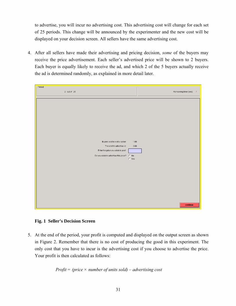
only one unit of the good each period. The good costs you nothing to produce. 2. At the beginning of every period, you decide on what price to charge per unit of good X and

whether or not you wish to advertise this price. See Figure 1 on the next page. Click on the Continue button to submit your price and advertising decision. The computer will wait until all sellers have made their decisions before displaying anyone’s price to the market.

3. If you choose to advertise the price then you must pay an advertising cost. If you choose not

31

to advertise, you will incur no advertising cost. This advertising cost will change for each set of 25 periods. This change will be announced by the experimenter and the new cost will be displayed on your decision screen. All sellers have the same advertising cost.

4. After all sellers have made their advertising and pricing decision, some of the buyers may

receive the price advertisement. Each seller’s advertised price will be shown to 2 buyers. Each buyer is equally likely to receive the ad, and which 2 of the 5 buyers actually receive the ad is determined randomly, as explained in more detail later.

Fig. 1 Seller’s Decision Screen

5. At the end of the period, your profit is computed and displayed on the output screen as shown

in Figure 2. Remember that there is no cost of producing the good in this experiment. The only cost that you have to incur is the advertising cost if you choose to advertise the price. Your profit is then calculated as follows:

Profit = (price × number of units sold) – advertising cost

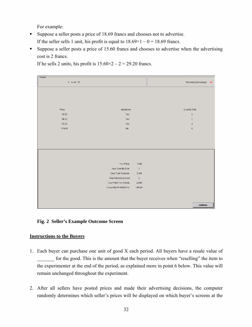
32

For example: Suppose a seller posts a price of 18.69 francs and chooses not to advertise.

If the seller sells 1 unit, his profit is equal to 18.69×1 – 0 = 18.69 francs. Suppose a seller posts a price of 15.60 francs and chooses to advertise when the advertising

cost is 2 francs. If he sells 2 units, his profit is 15.60×2 – 2 = 29.20 francs.

Fig. 2 Seller’s Example Outcome Screen

Instructions to the Buyers 1. Each buyer can purchase one unit of good X each period. All buyers have a resale value of

_______ for the good. This is the amount that the buyer receives when “reselling” the item to the experimenter at the end of the period, as explained more in point 6 below. This value will remain unchanged throughout the experiment.

2. After all sellers have posted prices and made their advertising decisions, the computer

randomly determines which seller’s prices will be displayed on which buyer’s screens at the

33

start of the buying phase of each period. That is, which price ad(s) the buyer receives is randomly determined and does not depend on the actions of the either buyers or the sellers. Note that some buyers may receive multiple ads and some may not receive any ad at all. The number of buyers who receive the ad depends on the number of sellers who advertise. For example, if one seller decides to advertise his price then two buyers will receive an ad. If two sellers decide to advertise, then there are 3 possibilities for the random ad distribution:

a. Two buyers get two ads each. b. One buyer gets two ads and two other buyers get one ad each. c. Four buyers get one ad each.

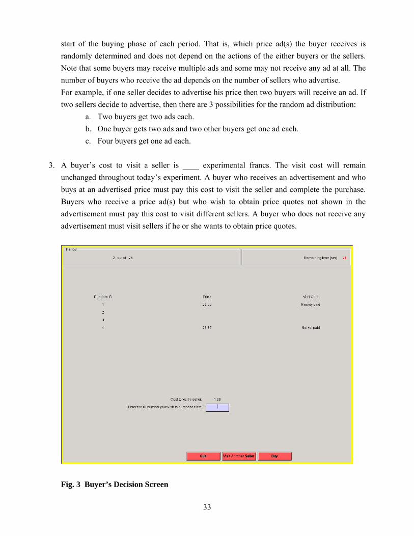
3. A buyer’s cost to visit a seller is ____ experimental francs. The visit cost will remain

unchanged throughout today’s experiment. A buyer who receives an advertisement and who buys at an advertised price must pay this cost to visit the seller and complete the purchase. Buyers who receive a price ad(s) but who wish to obtain price quotes not shown in the advertisement must pay this cost to visit different sellers. A buyer who does not receive any advertisement must visit sellers if he or she wants to obtain price quotes.

Fig. 3 Buyer’s Decision Screen

34

4. A buyer receives a new quote from a different, randomly-determined seller each time he or

she pays this visit cost by clicking the Visit Another Seller button on Figure 3. For example: a buyer who makes two visits to obtain price offers from two sellers will pay a total visit cost of _____ francs. If a buyer pays the visit cost to obtain a price quote from a particular seller in a certain period, he can purchase from that seller at any time during that same period without paying the visit cost again.

5. The prices are displayed on buyer’s computer screen as shown in Figure 3. The order of displayed prices is not related to the actual identity of the seller. The display order is randomly determined each period by the computer. To make the purchase, the buyer enters the temporary, random ID number of the seller from whom he wishes to make the purchase and then clicks on the Buy button. A buyer who chooses to visit another seller should click on the Visit Another Seller button. At any time, the buyer can choose not to purchase in the current period by clicking the Quit button.

6. At the end of the period, your profit is computed and displayed on an output screen similar to Figure 4. Remember that you will have to pay your visit cost irrespective of whether or not you buy the good. Your profit is then calculated as follows:

Profit (if you purchase) = resale value of the good – price paid – total cost of visiting sellers

Profit (if you do not purchase) = – total cost of visiting sellers

Note that a buyer would earn a negative profit (lose money) if she pays a price above the value of the good. For example: Suppose the resale value of the good is 20 and the cost of visiting a seller is 1. A buyer receives the ad from a seller with a quoted price of 10. • If he decides not to visit any other seller before buying, he earns Profit = 20 – 10 – 1= 9

(Note that he pays the visit cost of 1 to buy from a seller from whom he received an ad.) • If he decides to visit another seller and obtains a price quote of 15, he can purchase at one

of the two quoted prices, visit another seller or quit. o If he purchases at price 10, he earns Profit = 20 – 10 – 2 = 8. o If he decides to quit and not purchase, he must still pay the visit cost he just

incurred to obtain the price quote of 15. Therefore, he earns a negative profit of –1. o If he visits another seller and receives a quote of 6 and decides to purchase at this

price, he earns Profit = 20 – 6 – 2 = 12.

35

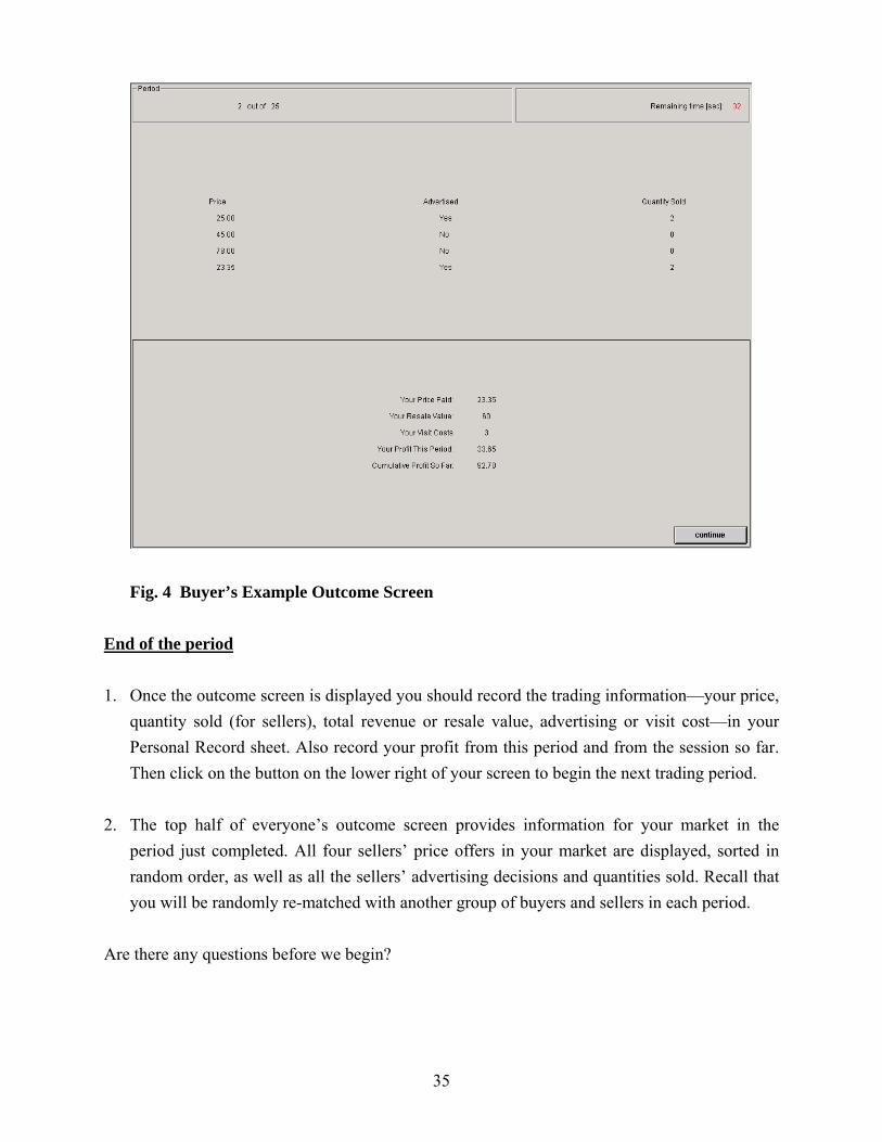
Fig. 4 Buyer’s Example Outcome Screen

End of the period

1. Once the outcome screen is displayed you should record the trading information—your price, quantity sold (for sellers), total revenue or resale value, advertising or visit cost—in your Personal Record sheet. Also record your profit from this period and from the session so far. Then click on the button on the lower right of your screen to begin the next trading period.

2. The top half of everyone’s outcome screen provides information for your market in the

period just completed. All four sellers’ price offers in your market are displayed, sorted in random order, as well as all the sellers’ advertising decisions and quantities sold. Recall that you will be randomly re-matched with another group of buyers and sellers in each period.

Are there any questions before we begin?

36

REFERENCES

Abrams, Eric, Martin Sefton and Abdullah Yavas (2000), An Experimental comparison of two search models, Economic Theory, Vol. 16, 735-749.

Baye, Michael, John Morgan and Patrick Scholten (2004), Price dispersion in the small and in the large: Evidence from an Internet price comparison site, Journal of Industrial Economics, Vol. 52, 463-496. Brown-Kruse, Jamie L., Stephen Rassenti and Stanley Reynolds and Vernon Smith (1994), Bertrand-Edgeworth Competition in Experimental Markets, Econometrica, Vol. 62, 343-371. Brynjolfsson, Eric and Michael Smith, (2000) “Frictionless commerce? A Comparison of Internet and Conventional Retailers," Management Science, Vol. 46, 563-585.

Burdett, Kenneth and Kenneth Judd (1983), Equilibrium Price Dispersion, Econometrica, Vol. 51, 955-970.

Cason, Timothy and Shakun Datta (2006), An Experimental Study of Price Dispersion in an Optimal Search Model with Advertising, International Journal of Industrial Organization, Vol. 24, 639-665.

Cason, Timothy and Daniel Friedman (2003), Buyer Search and Price Dispersion: A Laboratory Study, Journal of Economic Theory, Vol. 112, 232-260. Cason, Timothy, Daniel Friedman and Florian Wagener (2005), The Dynamics of Price Dispersion, or Edgeworth Variations, Journal of Economic Dynamics and Control, Vol. 29, 801-822. Cox, James and Ronald Oaxaca (1989), Laboratory Experiments with a Finite Horizon Job Search Model, Journal of Risk and Uncertainty, Vol. 2, 301-329. Cox, James and Ronald Oaxaca (2000), Good News and Bad News: Search from Unknown Wage Offer Distributions, Experimental Economics, Vol. 2, 197-225.

Davis, Douglas and Arlington Williams (1991), The Hayek Hypothesis in Experimental Auctions: Institutional Effects and Market Power, Economic Inquiry, Vol. 29, 261-274.

Diamond, Peter (1971), A Model of Price Adjustment, Journal of Economic Theory, Vol. 3, 156-168.

Fischbacher, Urs (2007), z-Tree: Zurich Toolbox for Readymade Economic Experiments, Experimental Economics, Vol. 10, 171-178.

Gale, Douglas (1988), Price Setting and Competition in a Simple Duopoly Model, Quarterly Journal of Economics, Vol. 103, 729-739.

37

Gronau, Reuben (1971), Information and Frictional Unemployment, American Economic Review, Vol. 61, 290-301. Harrison, Glenn and Patrick Morgan (1990), Search Intensity in Experiments, Economic Journal, Vol. 100, 478-486. Hey, John (1981), Are optimal search rules reasonable? And vice versa? (And does it matter anyway?), Journal of Economic Behavior and Organization, Vol. 2, 47-70. Hey, John (1982), Search for Rules for Search, Journal of Economic Behavior and Organization, Vol. 3, 65-81. Hopkins, Ed and Robert M. Seymour (2002), The Stability of Price Dispersion under Seller and Consumer Learning, International Economic Review, Vol. 43, 1157-1190. Lippman, Steven and John J. McCall (1976), The Economics of Job Search: A Survey – Part I, Economic Inquiry, Vol. 14, 155-189. McKelvey, Richard and Thomas Palfrey (1995), Quantal Response Equilibria for Normal Form Games, Games and Economic Behavior, Vol.10, 6-38. McKelvey, Richard and Thomas Palfrey (1995), Quantal Response Equilibria for Extensive Form Games, Experimental Economics, Vol.1, 9-41. . Morgan, John, Henrik Orzen, and Martin Sefton (2006a), An Experimental Study of Price Dispersion, Games and Economic Behavior, Vol. 54, 134-158.

Morgan, John, Henrik Orzen, and Martin Sefton (2006b), A Laboratory Study of Advertising and Price Competition, European Economic Review, Vol. 50, 323-347. Offerman, Theo, Jan Potters, and Joep Sonnemans (2002), Imitation and Belief Learning in an Oligopoly Experiment, Review of Economic Studies, Vol. 69, 973-997. Robert, Jacques and Dale O. Stahl (1993), Informative Price Advertising in a Sequential Search Model, Econometrica, Vol. 61, 657-686.

Salop, Steven (1973), Wage Differentials in a Dynamic Theory of the Firm, Journal of Economic Theory, Vol. 6, 321-344.

Schotter, Andrew and Yale M. Braunstein (1981), Economic Search: An Experimental Study, Economic Inquiry, Vol. 19, 1-25. Sonnemans, Joep (1998), Strategies of Search, Journal of Economic Behavior and Organization, Vol. 35, 309-322.

Stahl, Dale O. (1989), Oligopolistic Pricing with Sequential Consumer Search, American Economic Review, Vol. 79, 700-712.

38

Stahl, Dale O. (1996), Oligopolistic Pricing with heterogeneous consumer search, International Journal of Industrial Organization, Vol. 14, 243-268.

Stigler, George (1961), The Economics of Information, Journal of Political Economy, Vol. 69, 213-225.

Varian, Hal (1980), A Model of Sales, American Economic Review, Vol. 70, 651-659.

KRANNERT SCHOOL OF MANAGEMENT · Krannert School of Management Purdue ... Buyers then decide...

Documents

Transcript of KRANNERT SCHOOL OF MANAGEMENT · Krannert School of Management Purdue ... Buyers then decide...