Southern Illinois University CarbondaleOpenSIUC

Books, Monographs and Lecture Notes Department of Mathematics

1997

Knots and Links in Three-Dimensional FlowsRobert W. GhristUniversity of Texas at Austin

Philip J. HolmesPrinceton University

Michael C. SullivanSouthern Illinois University Carbondale, msulliva@math.siu.edu

Follow this and additional works at: http://opensiuc.lib.siu.edu/math_booksPart of the Mathematics Commons

Published in Knots and Links in Three-Dimensional Flows, Lecture Notes in Mathematics, volume1654. The original publication is available at www.springerlink.com.

This Article is brought to you for free and open access by the Department of Mathematics at OpenSIUC. It has been accepted for inclusion in Books,Monographs and Lecture Notes by an authorized administrator of OpenSIUC. For more information, please contact opensiuc@lib.siu.edu.

Recommended CitationGhrist, Robert W.; Holmes, Philip J.; and Sullivan, Michael C., "Knots and Links in Three-Dimensional Flows" (1997). Books,Monographs and Lecture Notes. Paper 1.http://opensiuc.lib.siu.edu/math_books/1

Knots and Links in Three-Dimensional FlowsR. W. Ghrist P. J. Holmes M. C. Sullivan

Dedicated to Robert F. Williams,teacher, colleague, and friend.

v

PrefaceThis book was envisaged in the Summer of 1992 at the NATO ASI Conferenceon Bifurcations of Periodic Orbits in Montreal. From genesis to completion,many new phenomena in the study of knots in dynamical systems have beenunearthed (as explored in Chapters 3 through 5).The authors have bene�tted from the support of several institutions, in-cluding Cornell's Center for Applied Mathematics, Princeton's Program in Ap-plied and Computational Mathematics, the Institute for Advanced Study, North-westen University, the University of Texas at Austin, and Southern Illinois Uni-versity at Carbondale. The authors gratefully acknowledge the support of theNational Science Foundation and the Department of Energy.Finally, we three are indebted to our colleagues who have provided inspirationand pointed out (hopefully most) errors in this text: these include Joan Birman,John Etnyre, John Franks, Jean-Marc Gambaudo, Alec Norton, Dan Silver, andBob Williams.

vi

Contents0 Introduction 10.1 The contents of this volume . . . . . . . . . . . . . . . . . . . . . 31 Prerequisites 51.1 The theory of knots and links . . . . . . . . . . . . . . . . . . . . 51.1.1 Basic de�nitions . . . . . . . . . . . . . . . . . . . . . . . 51.1.2 New knots from old . . . . . . . . . . . . . . . . . . . . . 81.1.3 Braid theory . . . . . . . . . . . . . . . . . . . . . . . . . 101.1.4 Numerical invariants . . . . . . . . . . . . . . . . . . . . . 121.2 The theory of dynamical systems . . . . . . . . . . . . . . . . . . 161.2.1 Basic de�nitions . . . . . . . . . . . . . . . . . . . . . . . 161.2.2 Symbolic dynamics . . . . . . . . . . . . . . . . . . . . . . 221.2.3 Bifurcations and one-dimensional maps . . . . . . . . . . 282 Templates 332.1 Branched manifolds and attractors . . . . . . . . . . . . . . . . . 342.2 Templates and the Template Theorem . . . . . . . . . . . . . . . 372.2.1 Case 1: a Markov owbox neighborhood . . . . . . . . . . 392.2.2 Case 2: the DA . . . . . . . . . . . . . . . . . . . . . . . . 422.3 Examples and applications . . . . . . . . . . . . . . . . . . . . . . 472.3.1 The Lorenz-like templates . . . . . . . . . . . . . . . . . . 472.3.2 Nonlinear oscillators, horseshoes, and H�enon maps . . . . 492.3.3 Shil'nikov connections . . . . . . . . . . . . . . . . . . . . 512.3.4 Fibred knots and links . . . . . . . . . . . . . . . . . . . . 542.3.5 Templates from time series . . . . . . . . . . . . . . . . . 572.4 A symbolic language . . . . . . . . . . . . . . . . . . . . . . . . . 602.4.1 Markov structures and symbolic coordinates . . . . . . . . 602.4.2 Subtemplates and template in ations . . . . . . . . . . . 633 Template Theory 693.1 Knotted orbits on templates . . . . . . . . . . . . . . . . . . . . . 693.1.1 Alexander's Theorem for templates . . . . . . . . . . . . . 693.1.2 Concatenation of template knots . . . . . . . . . . . . . . 703.1.3 The existence of knots on a template . . . . . . . . . . . . 733.1.4 Accumulations of knots . . . . . . . . . . . . . . . . . . . 753.2 Universal templates . . . . . . . . . . . . . . . . . . . . . . . . . 783.2.1 Examples of subtemplate structures . . . . . . . . . . . . 783.2.2 A template containing all links . . . . . . . . . . . . . . . 833.2.3 Universal templates . . . . . . . . . . . . . . . . . . . . . 89vii

viii CONTENTS3.2.4 Where do all the knots live? . . . . . . . . . . . . . . . . . 953.3 Subtemplate structures . . . . . . . . . . . . . . . . . . . . . . . . 973.3.1 Orientable subtemplates . . . . . . . . . . . . . . . . . . . 983.3.2 Nonorientable subtemplates . . . . . . . . . . . . . . . . . 1034 Bifurcations 1074.1 Local bifurcations and links . . . . . . . . . . . . . . . . . . . . . 1084.2 Torus knots and bifurcation sequences . . . . . . . . . . . . . . . 1124.2.1 Horseshoe torus knots . . . . . . . . . . . . . . . . . . . . 1154.2.2 Bifurcation reversal in the H�enon map . . . . . . . . . . . 1194.3 Self-similarity and horseshoe cables . . . . . . . . . . . . . . . . . 1214.3.1 Kneading factorization and subtemplates . . . . . . . . . 1224.3.2 Nested periodic orbits and iterated torus knots . . . . . . 1274.4 Homoclinic bifurcations . . . . . . . . . . . . . . . . . . . . . . . 1294.4.1 Gluing and torus knots . . . . . . . . . . . . . . . . . . . 1294.4.2 Silnikov connections and universal templates . . . . . . . 1345 Invariants 1435.1 Classifying suspended subshifts . . . . . . . . . . . . . . . . . . . 1455.1.1 Finitely generated Abelian groups . . . . . . . . . . . . . 1485.2 Orientation data and stronger invariants . . . . . . . . . . . . . . 1495.2.1 Additional Examples . . . . . . . . . . . . . . . . . . . . . 1525.3 Zeta functions and ows . . . . . . . . . . . . . . . . . . . . . . . 1545.3.1 Review of Zeta Functions . . . . . . . . . . . . . . . . . . 1545.3.2 Positive Ribbons . . . . . . . . . . . . . . . . . . . . . . . 1555.3.3 Counting Twisted Ribbons . . . . . . . . . . . . . . . . . 1575.4 A zeta function for Lorenz attractors . . . . . . . . . . . . . . . . 1595.5 Remarks on other invariants and open problems . . . . . . . . . . 1656 Concluding Remarks 167A Morse-Smale / Smale Flows 171A.1 Morse-Smale ows . . . . . . . . . . . . . . . . . . . . . . . . . . 171A.1.1 Round handles . . . . . . . . . . . . . . . . . . . . . . . . 173A.1.2 The 3-sphere . . . . . . . . . . . . . . . . . . . . . . . . . 175A.1.3 Wada's Theorem . . . . . . . . . . . . . . . . . . . . . . . 178A.1.4 Extensions and applications . . . . . . . . . . . . . . . . . 180A.2 Smale ows, abstract . . . . . . . . . . . . . . . . . . . . . . . . . 181A.3 Smale ows, embedded . . . . . . . . . . . . . . . . . . . . . . . . 185A.3.1 Lorenz templates . . . . . . . . . . . . . . . . . . . . . . . 188

Chapter 0: IntroductionThis book concerns knots and links in dynamical systems.Knot and link theory is an appealing subject. The basic ideas and results maybe appreciated intuitively, simply by playing with pieces of string (e.g.[11, 1]).Nonetheless, in spite of seafarers' development of sophisticated knots over thou-sands of years, the mathematical theory of knots began only in the nineteenthcentury. Its origins lie in Gauss's interest in electromagnetic �eld lines [67] and inattempts to classify knotted strings in the �ther, which Lord Kelvin and othersthought might correspond to di�erent chemical elements [176, 174]. It rapidlyshed its physical origins and became a cornerstone of low-dimensional topology.The roots of dynamical systems theory are considerably older and more tan-gled; they may be found in the Principia Mathematica of Isaac Newton and inattempts to model the motions of heavenly bodies. Ab initio the subject requiresmore technical apparatus: the di�erential and integral calculus, for a start; butat the same time it has kept closer touch with its physical origins. Moreover, inthe last hundred years, it too has (re)acquired a strong geometrical avor. Infact it was in an assault on the (restricted) three body problem of celestial me-chanics [145], in response to the prize competition to celebrate the 60th birthdayof King Oscar II of Sweden and Norway, that Henri Poincar�e essentially inventedthe modern, geometric theory of dynamical systems. He went on to develop hisideas in considerable detail in Nouvelles Methodes de la M�ecanique Celeste [146].Today, following this work, that of the Soviet school, including Pontriagin, An-dronov, Kolmogorov, Anosov, and Arnol'd, and of Moser and Smale and theirstudents in the West, the subject has reached a certain maturity. Over the lasttwenty years, it has escaped from Mathematics Departments into the scienti�cworld at large, and in its somewhat ill-de�ned incarnations as \chaos theory"and \nonlinear science," the methods and ideas of dynamical systems theory are�nding broad application.The basic world of a dynamical system is its state space: a (smooth) mani-fold, M , which constitutes all possible states of the system, and a mapping or ow de�ned on M . In one of our principal motivating examples, systems of�rst order ordinary di�erential equations (ODEs), the vector �eld thus speci�edgenerates a ow �t :M !M; t 2 R. The general problem tackled by dynamicalsystems theorists is to describe �t geometrically, via its action on subsets of M .This implies classi�cation of the asymptotic behaviors of all possible solutions,by �nding �xed points, periodic orbits and more exotic recurrent sets, as well asthe orbits which ow into and out of them. In many applications �t also dependson external parameters, and the topological changes or bifurcations that occurin M as these parameters are varied, are also of interest. In studying these andrelated phenomena, one abandons the fruitless search for closed form solutions1

2 chapter 0. introductionin terms of elementary or special functions, and seeks instead qualitative infor-mation.Over the past decade, knot theory, once in the inner sanctum of pure math-ematics, has been leaking out into other �elds through several successful appli-cations. These range from molecular biology, involving topological structures ofclosed DNA strands [173], to physics, led by surprising connections with statis-tical mechanics [99] and quantum �eld theory [197, 14]. Likewise, over the pastten to �fteen years, several attempts have been made to draw knot theory anddynamical systems closer together. The key idea is simple: a closed (periodic)orbit in a three-dimensional ow is an embedding of the circle, S1, into thethree-manifold that constitutes the state space of the system, hence it is a knot.Similarly, a �nite collection of periodic orbits de�nes a link.Several natural questions immediately arise, directed at the following goal:given a ow, perhaps generated by the vector �eld of a speci�c ODE, describethe knot and link types to be found among its periodic orbits. Do nontrivialknots occur? How many distinct knot types are represented? How many of eachtype? Do well-known families, such as torus knots, algebraic knots, or rationaltangles, appear in particular cases? In any cases? Are there \new" familiesof knots and links which arise naturally in certain ows? Do Hamiltonian andother systems with conservation laws or symmetries support preferred families oflinks? Do \chaotic" ows contain inherently richer knotting than simple (Morse-Smale) ows? Indeed, how complicated can things get? { is there a single ODEamong whose periodic orbits can be found representatives of all knots and links?Such questions might occur to topologists. Indeed, it was R.F. Williams, in thecontext of a seminar on turbulence conducted in the Mathematics Departmentat Berkeley in 1976, who �rst conjectured that nontrivial knotting occurs in awell-known set of ODEs called the Lorenz equations [193].Dynamicists, in contrast, might seek to use knot and link invariants to de-scribe periodic orbits and so help them better understand the underlying ODEs.In a parametrised family of ows, for example, one can observe sequences ofbifurcations in which a simple invariant set containing, say, one or two periodicorbits, \grows" into a chaotic set of great complexity, containing a countablein�nity of periodic orbits. In many cases, the periodic orbits are dense in the setof interest; sometimes that set is a so-called strange attractor. The existence-uniqueness theorem for solutions of ODEs implies that, as periodic orbits deformunder parameter variation, they cannot intersect or pass through one another.Knot and link types therefore provide topological invariants which may be at-tached to families of periodic orbits. Can such invariants be used to identifyorbit genealogies { to trace the bifurcation sequences in which they arose? (Afavorite problem is to describe bifurcation sequences in the two-parameter familyof maps introduced by H�enon [83], which provides a model for Smale's famoushorseshoe map.) Can operations in which new knots are created from old, suchas composition and cabling, be associated with speci�c local bifurcations? Is thecomplexity of knotting related to other measures of dynamical complexity, such

0.1. the contents of this volume 3as topological entropy? Does knot theory provide �ner invariants than entropyfor the classi�cation of ows?Of course, since periodic orbits form knots only in three-dimensional ows,applications to dynamical systems in general are severely limited. Nonetheless,many of the rich and wonderful behaviors that currently engage dynamicistsare already manifest in three dimensions, and so it seems well worth applyingwhatever tools we can to this case. In any event, we hope the reader will �ndthe subject as beautiful, and attractive, as we do.0.1 The contents of this volumeThis book attempts to bring together two largely disparate and well developed�elds, which have thus far only met in the pages of specialised research journals.As such, it cannot substitute for a proper course or text in either �eld. Chapter1, to follow immediately, provides a rapid review of the principal aspects of knottheory and dynamical systems theory required for the remainder of the book.In Chapter 2 we develop the major tool which allows us to pass back and forthbetween hyperbolic ows and knots: the template. This was introduced (underthe name \knot holder") over twelve years ago in two papers of Birman andWilliams [23, 24]. In dynamical systems it is common to use Poincar�e or returnmaps to reduce a ow to a mapping on a manifold of one lower dimension. WhilePoincar�e maps preserve certain periodic orbit data, information on how theorbits are embedded in the ow is lost. The template preserves that information,and likewise reduces dimension. In Chapter 2 we develop a host of relatedtools: subtemplates, template in ations and renormalisations, and the symboliclanguage which allows us to manipulate templates and explore relations amongthem. We also introduce some of the particular (families of) templates whichwill concern us later.Equipped with our basic tools, in Chapter 3 we obtain some general results ontemplate knots and links, including the facts that, while speci�c templates maynot contain all knots and links, every template contains in�nitely many distinctknot types. We then describe a universal template, which does contain all (tame)knots and links, and which, moreover, arises rather naturally in certain classesof structurally stable three dimensional ows. In the �nal section, we explorethe \embedding problem:" the question of which templates can be embedded inother templates. By considering isotopic embeddings, we are able to recogniseuniversal templates hidden in ostensibly simpler ones.The fourth chapter concerns bifurcations and knots, and directly addressesthe kinds of dynamical systems questions raised in our opening paragraphs. Inparticular we focus on speci�c templates related to the H�enon mapping and thecreation of horseshoes. Here, in contrast to the limitless riches of Chapter 3,there are severe restrictions on links (all crossings are of one sign), which leadto uniqueness results and order relations on orbit creation in local bifurcations.We also explore knot types born in certain global or homoclinic bifurcations,by lifting the contrast between dynamically simple and dynamically complex

4 chapter 0. introductionbifurcations to the knot-theoretic level. In so doing, we derive a rather generalset of suÆcient conditions for a third-order ODE to support all links as periodicorbits.Chapter 5 returns to basic template theory and presents the current stateof a�airs in template classi�cation and invariant theory. We commence witha discussion of what a sensible de�nition of template equivalence should be,based on intuition developed in Chapters 3 and 4, and continue with a primitivebut useful invariant: a zeta-function for a restricted class of templates. Thiswill be seen to relate nicely to the underlying symbolic dynamics, yielding aneasily-computed invariant which encodes \twisting" information in the compactpackage of a rational function.Chapter 6 is comprised of a short list of concluding remarks and open pro-belms that pertain to template theory and its applications.Throughout Chapters 2-5 we strive to present, for the �rst time, a fairlycomplete picture of the theory of templates. As such, we include key resultsof Franks, Birman, Williams and others, although we focus primarily on ourown work, relegating to an appendix some related work beyond the immediatescope of this monograph. Accordingly, Appendix A contains brief reviews ofwork by Morgan, Wada, and others on nonsingular Morse-Smale ows on three-manifolds, which contain only limited classes of knots. This is then contrastedwith the work of Franks and work in progress by Sullivan on nonsingular Smale ows on the three-sphere.Despite the title, we in no way claim to include every major result in theoverlap of dynamics and knot theory. In particular, there is a natural dichotomybetween knots arising from suspended surface homeomorphisms and those aris-ing as closed orbits in ows on three-manifolds: this text focuses on the lattersituation. The forthcoming book by P. Boyland and T. Hall [31] deals with theformer | there is a great deal of beautiful work being done in this area: Nielsentheory and \braid types" for surface automorphisms [30, 29]. In addition, knottheory intersects with dynamics in examining problems of integrable Hamilto-nian systems [50], the existence of minimal ows on three-manifolds [79] andcontact geometry [45]. Finally, analogues of knotting and linking for nonperi-odic, minimal orbits [15, 116] and \asymptotic" linking of orbits [64, 62] are veryexciting, particularly since there are applications to magnetohydrodynamics [7]and uid mechanics [129].

Chapter 1: PrerequisitesBefore introducing the tools for examining knotted periodic orbits in ows, weprovide a concise review of relevant de�nitions, ideas, and results from the topo-logical theory of knots and links and the dynamical theory of ows in threedimensions. This provides a language for describing phenomena, as in: a period-doubling bifurcation gives rise to a (2; n) cabling.Our treatment of both of these (large) bodies of theory is necessarily brief; wewish merely to describe the main ideas to be used in subsequent chapters. Severalgood references exist for these growing �elds. Standard texts for the theory ofknots and links includes the books by Rolfsen [154], Burde and Zieschang [33],and Kau�man [101]. In the theory of dynamical systems, a wealth of goodbooks can be found, including those by Robinson [153], Shub [162], Arnold [6],and Bowen [26]. Devaney's book [41] is a good introductory text on iteratedmappings. A more applied viewpoint can be found in the texts by Guckenheimerand Holmes [76] or Arrowsmith and Place [9].1.1 The theory of knots and linksGiven a piece of string, one may tie it up into all sorts of complicated knots.Nevertheless, as long as the ends are free, the mess may be untied completely(though in practice this may be frustrating!). If one should join the two freeends of the string together, then (intuitively) a knotted loop remains knotted nomatter how one tries to undo it. This is the idea behind knot theory.1.1.1 Basic de�nitionsDe�nition 1.1.1 A knot is an embedding K : S1 ,! S3 of a 1-sphere into the3-sphere. A link L :`S1 ,! S3 is a disjoint, �nite collection of knots.The three-sphere S3 is de�ned as the unit sphere in R4. The reader whois uncomfortable with S3 may replace it by R3 without loss, since S3 can beconsidered as R3 with an additional \point at in�nity." The simplest knot isthe unknot, pictured in Figure 1.1(a). An unknot is any embedding of S1 in S3whose image is the boundary of an embedded disc D2 � S3. The next \sim-plest" knots1 are the trefoil knot and the �gure-eight knot depicted in Figure 1.1.We will usually consider knots and links which are oriented, as depicted by an1The �rst knot theorists tabulated knots according to the minimal number of crossings in aplanar projection. In these tables (see [154] or [33]) the knots of Figure 1.1 are simplest: i.e.,they have the fewest possible number of crossings. Other notions of \simplicity" are of coursepossible [115]. 5

6 chapter 1. prerequisites(b) (c)(a)Figure 1.1: (a) the unknot; (b) the trefoil knot; (c) the �gure-eight knot.arrow along the knot in a diagram. Given some regular (i.e., transverse) planarrepresentation of an oriented knot or link, each crossing point has an inducedorientation, given by the convention of Figure 1.2. While our convention is op-posite that which is standard in knot theory, it has prevailed in the study ofknots in dynamical systems [23, 24, 93, 88, 89, 70].

+ �Figure 1.2: Sign convention for crossings.The fundamental problem of knot (link) theory is the following: when are twoknots (links) the same? In knot theory, the notion of \sameness" is constructedto match our intuition of deforming loops of knotted string.De�nition 1.1.2 Two knots K and ~K are ambient isotopic if there exists acontinuous one-parameter family ht of homeomorphisms of S3 such that h0 isthe identity map and h1 ÆK = ~K.Remark 1.1.3 The natural analogue of De�nition 1.1.2 holds for embeddingsof spaces in S3 other than S1, e.g., surfaces and solids. When working withknots and links in S3, it is common to refer to ambient isotopic knots as beingisotopic, even though isotopy is technically a weaker equivalence when workingwith noncompact spaces [33]. We use the terms interchangeably to denote theequivalence of De�nition 1.1.2.Unless speci�ed explicitly, the term \knot" may refer to either the actualembedding, or the image of the embedding, or the entire isotopy class of embed-

1.1. the theory of knots and links 7dings. We will formulate most of the theory in terms of knots | generalizationsto links are automatic.Given De�nition 1.1.2, the fundamental problem of knot theory can be statedas follows:Problem 1.1.4 When are two knots isotopic?One of the �rst triumphs of knot theory was a reformulation of Problem 1.1.4from a global-topological problem to a local-combinatorial one due to Reide-meister [149]. Given a knot or link, consider all its presentations; that is, planarprojections with overcrossings and undercrossings marked as in Figure 1.1. Anypresentation may always be chosen such that it is regular, having only transversedouble-points.Theorem 1.1.5 (Reidemeister [149]) Two regular presentations correspond toisotopic links if and only if the diagrams are related by isotopy (�xing the cross-ing points) and by a �nite sequence of the three Reidemeister moves, given inFigure 1.3.R1 R2

R3Figure 1.3: The three Reidemeister moves: R1, R2, R3.Even with Theorem 1.1.5, Problem 1.1.4 is very diÆcult to solve; however,restricted versions of this problem have clean solutions.Consider the class of torus knots: that is, knots which lie on a torus T 2 =S1 � S1 � S3, where each S1 is unknotted. These knots are described by theirwinding number in the meridional and longitudinal directions. A type (m;n)torus knot (m and n relatively prime positive integers) is a simple closed curveon T 2 which winds about the longitudinal direction m times and about themeridional direction n times [154, 33].

8 chapter 1. prerequisitesExample 1.1.6 The trefoil knot of Figure 1.1(b) is a (2,3) torus knot.The family of torus knots is well-understood; in particular, we have:Proposition 1.1.7 ([154, 33]) Torus knots of type (m;n) and (m0; n0) are iso-topic if and only if m = m0 and n = n0 (or, equivalently, m = n0 and n = m0).1.1.2 New knots from oldOne possible method for building and classifying knots is to begin with a simplefamily (e.g., the torus knots) and combine its members in various ways. Giventwo knots, there are certain constructions for creating a new knot: we shallconsider two such operations which also have dynamical interpretations.Connected sumsThe �rst operation we consider is a form of \multiplication" for knots called,oddly enough, the sum.Figure 1.4: The connected sum of two knots.De�nition 1.1.8 Given two oriented knots K and ~K, their connected sum,K# ~K, is formed by placing each in disjoint embedded 3-balls, B and ~B, suchthat some closed arc of K ( ~K) lies on the boundary of B ( ~B resp.). Then, deletethe interior of each arc and identify the boundaries of the arcs via an orientationpreserving homeomorphism. See Figure 1.4 for an illustration.Remark 1.1.9 In De�nition 1.1.8, the choice of balls and arcs does not a�ectthe connected sum. This operation is commutative and associative, but is not agroup operation due to the lack of inverses [154].If a knot can be decomposed into the connected sum of two or more nontrivialknots, it is said to be composite, else it is prime. The torus knots, for example,are prime (a nice proof can be found in [33, pp. 92-93]. A classical theoremdue to Schubert states that every knot has a unique prime factorization as theconnected sum of prime knots. R. F. Williams and M. Sullivan have exploredthe presence of prime decompositions of periodic orbits of ows [195, 169].

1.1. the theory of knots and links 9Companions and satellitesIf one thinks of the connected sum as a form of multiplication on the space ofall knots (complete with prime factorization as with the integers), the operationof taking satellites is akin to taking powers. Let V � D2 � S1 be a solid toruswhich sits in S3 in the standard way. Let K be a knot essentially embedded inV , i.e., K is not contained in any 3-ball B � V . Let ~K be an arbitrary knot andN ~K a tubular neighborhood of this knot in S3. A homeomorphism h : V ! N ~Kis said to be faithful if it takes the longitude of @V to a longitude of @N ~K whichis homologically trivial (it bounds a surface) in the complement S3 nN ~K .De�nition 1.1.10 The image of K under a faithful homeomorphism h is asatellite knot with companion ~K and pattern (K;V ): see Figure 1.5. IfK isotopesto a subset of @V � T 2, then K is a (p; q) torus knot and h(K) is said to be the(p; q) cable of ~K.~KV K h h(K)

h(V )Figure 1.5: A companion ( ~K) and a satellite (h(K)) knot.If we take ~K to be the unknot, a (p1; q1) cable of ~K is a (p1; q1) torus knot. Ifwe build a (p2; q2) cable of this torus knot, we obtain a new knot. By continuingthis procedure, with (pi; qi) cablings at each step, one produces an iterated torusknot of type f(pi; qi)gni=1. Alternatively, we say that the set of knots generatedfrom the unknot by the operation of cabling is called the set of iterated torus

10 chapter 1. prerequisitesknots. Following Fomenko and Nguyen [50], we will denote the set of knotsgenerated from the unknot by the operations of cabling and connected sum theset of generalized iterated torus knots. Both of these families of knots arisenaturally in a dynamical context as shown in Appendix A.1.1.3 Braid theoryKnot and link theory studies embeddings of circles in S3. With some slightrestrictions on the range of the embeddings, one can also embed arcs in topo-logically distinct ways. Braid theory studies these phenomena (see [19, 81]):De�nition 1.1.11 Given N a positive integer, a braid on N strands is a collec-tion b = fbigN1 of N disjoint embeddings of the interval [0; 1] into Euclidean R3such that for each i,1. bi(0) = (i; 0; 1);2. bi(1) = (�(i); 0; 0) for some permutation � ; and3. p3[bi(t)] is a monotone decreasing function of t, where p3 denotes projectiononto the third coordinate.De�nition 1.1.12 Two braids, b and ~b, are isotopic if there exists an isotopyht from b to ~b as per De�nition 1.1.2 and if ht Æ b satis�es De�nition 1.1.11 forall t 2 [0; 1].The study of braids di�ers from the study of knots chie y in that there is anatural group structure on the set of braids. Restricting to the set of all braidson N strands, there is a group operation given by concatenation. Given braidsb and ~b, one forms the braid sum b~b by appending the top of the ith strand of~b to the bottom of the ith strand of b: see Figure 1.6. In this way, one obtainsthe braid group on N strands, BN .

Figure 1.6: The sum operation on the braid group B3: �21�2 concatenated with��11 �2 equals �21�2��11 �2.

1.1. the theory of knots and links 11The standard generators for BN are denoted f�i : i = 1:::(N � 1)g and aregiven geometrically as the crossing of the ith strand over the (i + 1)st strand,as depicted in Figure 1.7. The presentation for BN under these generators wasgiven by Artin [10] to be the following:BN = ��1; �2; : : : ; �N�1 : �i�j = �j�i ; ji� jj > 1�i�i+1�i = �i+1�i�i+1 ; i < N � 1 � : (1.1)The relations for this presentation are illustrated in Figure 1.8.�1 ��13Figure 1.7: Examples of generators for the braid group B4.

(a) (b)Figure 1.8: Relations for the braid group BN : (a) �i�j = �j�i for ji � jj > 1;(b) �i�i+1�i = �i+1�i�i+1 for i < N � 1.A relationship between braid theory and link theory is established by a simpleoperation on braids known as closure. Given a braid b, one forms a closed braid, b,by connecting the top and the bottom of each strand of b in the obvious fashion:see Figure 1.9. The question of the extent to which closed braids represent knotsand links was answered by Alexander [3]:

12 chapter 1. prerequisites

(b)(a) (c)Figure 1.9: (a) the braid �21�2; (b) its closure; (c) this is isotopic (via the �rstReidemeister move) to the Hopf link.Theorem 1.1.13 (Alexander [3]) Any link L is isotopic to a closed braid onsome number of strands.To understand the proof of Theorem 1.1.13, the reader is encouraged to isotopea closed piece of string into a closed braid: choose a provisional braid axis, aboutwhich the strands should revolve, and then try to maneuver the strands into aclosed braid. One naturally uses certain \moves" which are detailed in the proof(see [33, 19].We will make use of closed braids in Chapter 3 as a way to build knots andlinks, thanks to Theorem 1.1.13.Certain classes of braids and closed braids will be prevalent in our treatmentof knots and links. A braid b 2 Bn will be called positive if b, as a word inthe generators f�ig, contains either no inverses or all inverses, i.e., either allcrossings in the braid are positive, in the sign convention of Figure 1.2, or allare negative.2 A link L will be called positive if L has a representation as theclosure of a positive braid.Remark 1.1.14 There exist knots with diagrams containing only positive cross-ings, but which are not positive braids [182]. The proof is nontrivial, and usesthe Alexander-Conway polynomial | a link invariant.1.1.4 Numerical invariantsThe equivalence problem (Problem 1.1.4) for knots and links is extremely diÆcultand has not yet been solved in a computationally reasonable manner. However,2The term positive is used in both cases, either all positive crossings or all negative crossings.We �nd this confusing and would prefer the term uniform; however, we yield to the commonpractice in the remainder of this work.

1.1. the theory of knots and links 13many advances have been made through the use of algebraic invariants (see[101, 99, 20, 21, 94, 59] for examples). Here we merely describe some simpler,classical, numerical invariants, which will suÆce for out purposes.A numerical invariant is a well-de�ned function from link equivalence classesto the integers. For example, the function which maps a link L to the numberof its components �(L) is obviously invariant under isotopy, and hence de�nesa numerical invariant. However, this invariant has rather poor eyesight, since itdoes not distinguish di�erent n-component links.Consider a link L of two components,K and ~K. There is a well-de�ned notionof how \entwined" K and ~K are, encoded in the linking number, `k(K; ~K) 2 Z.There are numerous ways to de�ne linking number [154], the simplest of whichinvolves a presentation of the link (recall Theorem 1.1.5). For an oriented link,one can label each crossing of a regular link presentation with an integer �1, asper the convention of Figure 1.2.De�nition 1.1.15 Given two knots K and ~K, the linking number, `k(K; ~K), isgiven as half the sum of the signs over all crossings of K with ~K,`k(K; ~K) = 12 XK\ ~K �i; (1.2)where �i = �1 is the sign of the ith crossing and K \ ~K denotes the crossings ofK and ~K in some regular presentation.Lemma 1.1.16 Linking number is a link isotopy invariant.Proof: By Theorem 1.1.5, isotopy is generated by the Reidemeister moves ofFigure 1.3. It is easy to verify that linking number does not change under theselocal moves. 2The linking number `k(K; ~K) is related to the intuitive notion of linking.For example, de�ne a separable link to be one for which there exists a smoothembedded 2-sphere S2 in S3 which separates one (or more) component(s) of Lfrom the remainder of L. Any two separated components of a link are said tobe unlinked, and, indeed, their linking number must be zero, since there existsa presentation for the link in which the components do not cross at all. Wenote, however, that it does not follow that two knots with linking number zeroare necessarily separated: see the Whitehead link of Figure 2.16 for a classicalexample.One of the most important numerical invariants is the genus of a link. Recallthat closed orientable surfaces are classi�ed by genus, or the number of handles ina handlebody decomposition. Similarly, the genus of any surface with boundaryis de�ned as the genus of the surface obtained by abstractly gluing in a discalong each boundary component.De�nition 1.1.17 Given a link L, the genus, g(L), is de�ned as the minimumgenus over all orientable surfaces S which span L: that is, @S = L, where @S

14 chapter 1. prerequisitesis the oriented boundary. A spanning surface of minimal genus is known as aSeifert surface.Genus is by de�nition an invariant. Since by de�nition a knot in S3 bounds adisk if and only if it is the unknot, then among knots, only the unknot may havegenus zero.There are numerous formulae available for computing genera of links. Weinclude one, due to Birman and Williams [23], following work of Stallings [167],which will be particularly useful in later chapters.Theorem 1.1.18 (Birman and Williams [24]) Let L be a non-separable link of� components, presented as a closed positive braid on N strands, with c crossings.Then g(L), the genus of L, is given asg(L) = c�N � �2 + 1: (1.3)Example 1.1.19 In Figure 1.10(a), we show the trefoil knot along with a span-ning surface. An Euler number calculation reveals that the surface is a puncturedtorus whose genus is one. By using Equation (1.3) on the (positive) braid repre-sentation in Figure 1.10(b), we get � = 1, c = +3; and N = 2; hence, the genusis one, and the surface of part (a) is actually the Seifert surface. This provesthat the trefoil is indeed knotted.

(a) (b)Figure 1.10: (a) A spanning surface for the trefoil knot; (b) a positive braidpresentationExample 1.1.20 We may extend the idea of Example 1.1.19 to compute ageneral formula for the genus of a torus knot. For K a (m;n) torus knot withm > n, we present a presentation of K as a positive braid in Figure 1.11:there are m strands on a cylinder (the logitudinal direction), n of which twist

1.1. the theory of knots and links 15around the back (the meridional direction). The closure of this braid is K. Itis an exercise for the reader to count the crossings in this illustration and, usingEquation (1.3), compute the genus of K to be:g(K) = (m� 1)(n� 1)2 : (1.4)

n m� nFigure 1.11: The (m;n) torus knot as a positive braid on m strands.Exercise 1.1.21 The �gure-8 knot has genus one and braid word �1��12 �1��12 .Show that it cannot be presented as a positive braid. Hint: use induction on thenumber of strands.Solution: Clearly, one or two strands will not suÆce. For three strands, theremust be precisely four crossings to ensure genus one. Show that any positivebraid with four crossings is either a trefoil or a link with more than one compo-nent. For N > 3 strands, c = N + 1, and, given a positive braid on N strandswith N + 1 crossings, there must be one braid generator that is only used once.Thus, by \ ipping" as in the �rst Reidemeister move, one can reduce the num-ber of strands while retaining positivity, and thus obtain a counter example onN � 1 strands. 2The condition of having a positive closed braid is crucial to Theorem 1.1.18.For non-positive (or mixed) braids, there exists an extension of Theorem 1.1.18due to Bennequin [17], who derived a lower bound for genera of closed braidsgiven the same data as in Theorem 1.1.18:33The upper bound follows from direct construction.

16 chapter 1. prerequisitesTheorem 1.1.22 (Bennequin [17]) Let L be a nonseparable link of � compo-nents, presented as a closed braid on N strands, with c+ (c�) crossings in thepositive (negative) sense. Then g(L), the genus of L, is bounded as follows:jc+ � c�j �N � �2 + 1 � g(L) � jc+ + c�j �N � �2 + 1: (1.5)There are numerous other classical numerical invariants for knots and links:we mention one last example for future reference.De�nition 1.1.23 Given a link L, the braid index of L, bi(L), is de�ned as theminimum number of strands over all closed braid representations of L.Again, this is an invariant by de�nition. Unfortunately, there does not exist ananalogue of Equation (1.3) for calculating braid index. Nevertheless, we will usethis invariant in Chapter 4.This brief treatment of knot and link theory does not even begin to recountthe major developments, especially in the areas of higher invariants (maps fromlink isotopy classes to algebraic objects with more structure than Z). Greatstrides have been made in discovering computable multi-variable polynomialinvariants which have excellent resolution [59].Equally as exciting are the insightsgained through the [continuing] development of �nite-type, or Vasiliev invariants[21, 22, 183]. Our (modest) goal in this section has been merely to acquaintthe unfamiliar reader with this beautiful subject. For a deeper understanding,the \classical" theory of knots and links is well-covered in [154, 33]. Newerperspectives can be found in [21] and the references therein. Braid theory iscovered in [19], with more recent progress reported in [20].1.2 The theory of dynamical systemsTopology is the study of continuous maps between topological spaces: f : X !Y . In the case where f : X ! X , one is easily persuaded to consider iteratedpoints or orbits of f . Dynamics seeks to understand asymptotic properties oforbits, be they orbits of maps (Z-actions) or of ows (R-actions). In the case of ows on 3-manifolds, we will consider the topological properties of closed orbitsas knots and links. But in order to proceed, we will need a certain amount ofterminology and theory for both maps and ows.1.2.1 Basic de�nitionsDiscrete dynamicsAlthough dynamical systems originated in questions about continuous-time dy-namics (in celestial mechanics; see, for example, the historical account in [43]),much of the theory was developed �rst for maps, as it is somewhat simpler inthis case. Thus, in this section, we assume f : M ! M is a di�eomorphism ofan n-manifold M . The orbit, o(x), of a point x 2 M is de�ned as the set ofiterates ffk(x) : k 2 Zg.

1.2. the theory of dynamical systems 17Remark 1.2.1 Although we state the results for di�eomorphisms, much of thetheory goes through for smooth noninvertible maps, for which one works withthe orbits ffk(x) : k 2 Ng. The case of one-dimensional noninvertible mapswill be of particular concern in Section 1.2.3, and subsequently in the study ofsemi ows on templates.There are two primary problems associated to the dynamics of maps. The �rstis the equivalence problem (cf. Problem 1.1.4):De�nition 1.2.2 Two di�eomorphisms f : M ! M and ~f : N ! N areconjugate if there exists a homeomorphism h : M ! N such that the followingdiagram commutes: M f�! Mh # # hN ~f�! N (1.6)Problem 1.2.3 When are two di�eomorphisms conjugate?The second principal problem of dynamics concerns stability: when are all\nearby" maps equivalent?De�nition 1.2.4 A di�eomorphisms f : M ! M is structurally stable if alldi�eomorphisms in a suÆciently small neighborhood of f in C1(M) are conjugateto f .Problem 1.2.5 When is a map structurally stable?Problems 1.2.3 and 1.2.5 are relevant, not only to the study of maps and ows(to be discussed below), but also to the physical processes that are frequentlymodeled by such systems. They are large problems, whose study has spawned anumber of important results and perspectives.We begin by breaking the problem down. An invariant set of f is a subset� � M such that f(�) = �. An equilibrium, or �xed point for f is a one-pointinvariant set. Understanding of the behavior on an invariant set � is greatlyfacilitated if the action of f on � can be decomposed into uniformly expandingand contracting pieces. This is the kernel of the notion of hyperbolicity.De�nition 1.2.6 An invariant set � � M for a map f : M ! M is hyperbolicif there exists a continuous f -invariant splitting of the tangent bundle TM� intostable and unstable bundles Es� �Eu� withkDfn(v)k � C��nkvk 8 v 2 Es�; 8 n > 0;kDf�n(v)k � C��nkvk 8 v 2 Eu�; 8 n > 0; (1.7)for some �xed C > 0; � > 1.If f is hyperbolic on all of M , we say that f is Anosov. Given a hyperbolicstructure on an invariant set, the dynamics and stability of orbits on that pieceare well-understood, as we now describe.

18 chapter 1. prerequisitesExample 1.2.7 (the toral Anosov map) Consider the linear map f : R2 !R2 given by f : � xy � 7! � 2 11 1 �� xy � = � 2x+ yx+ y � : (1.8)The point (0; 0) is an equilibrium point which is hyperbolic since Df acts onthe tangent plane with the same linear map, and this map has eigenvalues andeigenvectors �u;s = 32 � 52p2 ; vu;s = � 112 � 12p5 � : (1.9)Thus, the map f has expanding (unstable) and contracting (stable) bundles, Euand Es, along the span of each eigenvector. Notice that the map f preserves theinteger lattice; hence, we may consider f as a map on R2=Z2, i.e., the torus T 2.Since f has determinant 1, the induced map on T 2 is invertible. While the actionof f on R2 is rather bland, its action on T 2 is quite interesting: the stable andunstable directions (Es and Eu) have irrational slopes, so these project down toinvariant manifolds on T 2 which wind about the torus densely: see Figure 1.12.Furthermore, the periodic points of f on T 2 are dense, since any pair of rationalnumbers with the same denominator gives the coordinates of a periodic point.f

Figure 1.12: The action of the map f on T 2.Remark 1.2.8 The map of Example 1.2.7 is hyperbolic on all of T 2, hence itis Anosov. We will return to this toral Anosov map in x2.3.4.Notice in Example 1.2.7 that the stable and unstable bundles in the tangentspace are mimicked in the base space by invariant manifolds (the projection ofEs and Eu) on which the map is uniformly contractive or expansive. For a mapon M with a hyperbolic structure on some invariant set �, the splitting of the

1.2. the theory of dynamical systems 19tangent bundle TM� into invariant stable and unstable bundles projects downto give invariant stable and unstable manifolds in M . This is the content of oneof the key results of this �eld: the Stable Manifold Theorem.4Theorem 1.2.9 (The Stable Manifold Theorem: Hirsch, Pugh, and Shub[84]) Given a di�eomorphism f :M !M with a hyperbolic invariant set �, foreach x 2 �, the setsW s(x) = fy 2M : limn!1 kfn(y)� fn(x)k = 0g ;W u(x) = fy 2M : limn!�1 kfn(y)� fn(x)k = 0g ; (1.10)are smooth, injective immersions of the bundles Esx and Eux respectively. Inaddition, W s(x) and W u(x) are tangent to the bundles at x: T (W s(x))x = Esxand T (W u(x))x = Esx. The sets W s(x) and W u(x) are known as the stable andunstable manifolds of x.Remark 1.2.10 The notion of local stable and unstable manifolds is also useful.Given f as in Theorem 1.2.9, the local stable and unstable manifolds are de�nedas: W sloc(x) = fy 2M : limn!1 kfn(y)� fn(x)k = 0and kfn(y)� fn(x)k < � 8n � 0g ;W uloc(x) = fy 2M : limn!�1 kfn(y)� fn(x)k = 0and kfn(y)� fn(x)k < � 8n � 0g ; (1.11)for � of \appropriately" small size.5 Theorem 1.2.9 then states that W sloc(x) andW uloc(x) are tangent to Esx and Eux .Theorem 1.2.9 is a very strong result, which we will rely upon frequentlyto describe the dynamics on a hyperbolic invariant set. The real issue thenis ascertaining the smallest invariant subset of M which contains \all" of theessential dynamics of the ow, and then considering systems in which this pieceis hyperbolic. Through work of Smale, Shub, and others [165, 162], we knowthis essential piece to be the chain-recurrent set.De�nition 1.2.11 Given a map f :M !M , a point x 2M is chain-recurrentfor f if, for any � > 0, there exists a sequence of points fx = x1; x2; : : : ; xn�1; xn =xg such that kf(xi) � xi+1k < � for all 1 � i � n� 1. The chain-recurrent set,R(f), is the set of all chain-recurrent points on M .Remark 1.2.12 The chain-recurrent set R(f) is closed and invariant.When one has a hyperbolic chain-recurrent set, there is a sort of prime decom-position theorem for the associated dynamics:4The Stable Manifold theorem was proved in stages, by several authors, starting with thecases of � a �xed point or periodic orbit. Theorem 1.2.9 is a rather general statement.5There is some ambiguity about the size of � { an appropriate size is usually clear from thecontext.

20 chapter 1. prerequisitesTheorem 1.2.13 (Smale [165]) Given a di�eomorphism f : M ! M havinga hyperbolic chain-recurrent set, R(f) is the union of disjoint basic sets, Bi,i = 1; 2; : : : ; N . Each Bi is closed, invariant, and contains a dense orbit. Theperiodic orbit set of each Bi is dense within Bi.In later chapters, we will often deal with systems which have hyperbolicchain-recurrent sets of various types. One more condition is often required: amap is said to satisfy the strong transversality condition if, for all x; y 2 R(f), thestable and unstable manifolds,W s(x) andW u(y), are transverse. This conditionis important in the de�nition of Morse-Smale and Smale di�eomorphisms. ASmale di�eomorphism is one which has a zero-dimensional hyperbolic chain-recurrent set satisfying the strong transversality condition, while a Morse-Smaledi�eomorphism is a Smale di�eomorphism for which the chain-recurrent set is�nite.Working with hyperbolic chain-recurrent sets and transversality has permit-ted a partial solution of the stability problem (Problem 1.2.5):Theorem 1.2.14 (Robbin [150], Robinson [151]) Any di�eomorphism f :M !M having a hyperbolic chain-recurrent set and satisfying the transversality con-dition, is structurally stable.Continuous dynamicsA map can be considered as a Z-action on M . A continuous analogue to a mapis an R-action, or a ow.De�nition 1.2.15 A ow on a manifoldM is a continuous map � : R�M !Msatisfying the following conditions:1. �t � �(t;�) :M !M is a homeomorphism of M for all t;2. �0 = idM , that is, �0(x) = x for all x 2M ;3. �t(�s(x)) = �t+s(x) for all s; t 2 R.While ows and maps are fundamentally di�erent objects, in certain in-stances they can be related. Given a map f : M ! M , one can de�ne thesuspension ow of f to be the quotient space of M � R with the trivial ow�t(x; s) = (x; s + t) via identifying (x; s) with (f(x); s + 1). The ow �t passesto a suspension ow, ~�t, acting on the mapping torus, ~M = M � R=(x; s) �(f(x); s + 1). In the case where f is isotopic to the identity map, ~M is homeo-morphic to M � S1, hence the name.Conversely, given a ow t on a closed manifold S, we say that S has alocal cross section (or Poincar�e section) if there exists a closed codimension-onesubmanifold � � S which transversely intersects the ow at every point of �. Inthe case where some subset U � � consists of orbits which return to � in �nitetime, there is a well-de�ned return map (or Poincar�e map) r : U ! � whichassigns to a point p 2 U the image T (p)(p), where T (p), the return time, is thesmallest t > 0 such that t(p) 2 �. In the case where � intersects all ow lines

1.2. the theory of dynamical systems 21of �t, we say that � is a global cross section. Clearly, taking the (appropriate)Poincar�e section is the inverse of suspending a map. The study of iteratedmappings assumed its central importance in dynamics after Poincar�e developedthe technique of cross-sections and return maps to study periodic orbits in owsgenerated by ordinary di�erential equations: examples appear throughout theremainer of this text, most notably in Chapter 4.When passing to ows, many of the de�nitions of x1.2.1 carry over with theobvious modi�cations: e.g., invariant sets, periodic orbits, etc. A few de�nitionsrequire additional explanation:De�nition 1.2.16 An invariant set � for a ow �t on M is hyperbolic if thereexists a continuous �t-invariant splitting of the tangent bundle TM� into Es� �Eu� �Ec� with kD�t(v)k � Ce��tkvk 8 v 2 Es�; 8t > 0;kD��t(v)k � Ce��tkvk 8 v 2 Eu�; 8t > 0; (1.12)d�tdt ����t=0(x) spans Ecx 8x 2 �;for some �xed C > 0; � > 1. The one-dimensional \center" direction Ecx istangent to the orbit itself at each point.De�nition 1.2.17 Let X � � be a subset of a hyperbolic invariant set of a ow �t on M . Then the stable and unstable manifolds of X in M are given byW s(X) = fy 2M : limt!1 k�t(X)� �t(y)k = 0g ;W u(X) = fy 2M : limt!�1 k�t(X)� �t(y)k = 0g : (1.13)The local stable and unstable manifolds of a set X are given by:W sloc(X) = fy 2M : limt!1 k�t(y)� �t(X)k = 0and k�t(y)� �t(X)k < � 8t � 0g ;W uloc(X) = fy 2M : limt!�1 k�t(y)� �t(X)k = 0and k�t(y)� �t(X)k < � 8t � 0g ; (1.14)For � an \appropriately" small positive number.Remark 1.2.18 Given a periodic orbit for a ow �t, the local stable andunstable manifolds can carry additional information. Consider the case where,say, W sloc( ) has dimension two: then, the local stable manifold is a ribboncontaining as a core. This ribbon is homeomorphic to either an annulus or aM�obius band, yielding an untwisted or twisted periodic orbit respectively. Weuse such information in x3.1, x4.1, and x5.3.De�nition 1.2.19 Given a ow �t onM , a point x 2M is chain-recurrent for �if, for any � > 0, there exists a sequence of points fx = x1; x2; : : : ; xn�1; xn = xgand real numbers ft1; t2; : : : ; tn�1g such that ti > 1 and k�ti(xi)�xi+1k < � forall 1 � i � n� 1. The chain-recurrent set, R(�), is the set of all chain-recurrentpoints on M .

22 chapter 1. prerequisitesThe Stable Manifold Theorem for ows is entirely analogous to Theorem1.2.9, and Theorem 1.2.13 holds as stated for ows with hyperbolic chain-recurrent sets. The de�nitions of Morse-Smale and Smale ows follows withone modi�cation: their chain-recurrent sets are one-dimensional, since these are ows. Hence, a Morse-Smale ow is a ow which has a �nite number of hyper-bolic �xed points and periodic orbits, all of whose stable and unstable manifoldsintersect transversally: see Appendix A.1.2.2 Symbolic dynamicsOne of the most remarkable { and fortunate { properties of complicated hyper-bolic invariant sets is the description they admit via symbolic dynamics. Thistheory has a long history, beginning with its use by Hadamard in describingclosed geodesics [80], and continuing in the work of Morse [133, 134].Shifts and subshiftsLet � = fx1; x2; : : : ; xNg be an alphabet of N letters. Denote by �N the spaceof bi-in�nite symbol sequences in �:�N = f: : : a�2a�1:a0a1a2 : : : : ai 2 �; 8i 2 Zg = �Z: (1.15)Points in �N will be called itineraries. The space �N is given the producttopology and can be endowed with a metric as follows. If a = (ai)1i=�1 andb = (bi)1i=�1 are itineraries, then the distance d(a;b) isd(a;b) = 1Xn=�1 Æ(n)2jnj ; where Æ(n) = � 0 : an = bn1 : an 6= bn : (1.16)Under this metric, points in �N are close when their symbol sequences agree onlarge blocks forwards and backwards from the \midpoint" a0.De�ne the shift map � : �N ! �N as follows:�(: : : a�2a�1:a0a1a2 : : :) = : : : a�1a0:a1a2a3 : : : : (1.17)Under the product topology, the shift map � is a homeomorphism. The dynam-ical system (�N ; �) is called the full N-shift.GivenA anN byN matrix of zeros and ones, an itinerary a = : : : a�1:a0a1 : : :is admissible with respect toA at i if, for aiai+1 = xjxk (where j; k 2 f1; 2; :::; Ng),A(j; k) = 1. Any itinerary a which is admissible with respect to A at all i iscalled admissible.De�nition 1.2.20 Given A an N by N matrix in zeros and ones, the subshift of�nite type associated with A is the dynamical system (�A; �), where �A � �N isthe set of admissible itineraries and � is the shift map. The matrix A is known asthe transition matrix for �A, since it speci�es those transitions between symbolsthat are possible within a sequence.

1.2. the theory of dynamical systems 23Example 1.2.21 Consider the subshift of �nite type associated with the tran-sition matrix A = 24 1 1 01 1 11 1 1 35 : (1.18)Then the system (�A; �) consists of all bi-in�nite sequences in fx1; x2; x3g notcontaining x1x3 as a subword.Remark 1.2.22 An alternative to De�nition 1.2.20 comes from graph theory.Let � be a directed (oriented) �nite graph with vertex set v = fvig and edgeset e = fejg, such that there exists at most one edge connecting any orderedvertex pair in v� v. Then the space of bi-in�nite, continuous, directed paths in� can be put in bijective correspondence with all bi-in�nite symbol sequences infvig admissible with respect to a transition matrix Av , where Av(i; j) = 1 if andonly if there is a continuous path from vi to vj . Alternatively, directed paths in� can also be represented by symbol sequences in the edge labels fejg, wherethe transition matrix Ae satis�es Ae(i; j) = 1 if and only if there the tip of theedge ei meets the tail of the edge ej . In general, these matrices, Av and Ae,will di�er. Thus, since the space of paths on � is the same, we have shown theexistence of di�erent subshifts which are nevertheless conjugate: see Figure 1.13.v1 v2 e1 e2Figure 1.13: The vertex graph (left) and the edge graph (right) associated tothe 2� 2 matrix A, where A(i; j) = 1 for all i; j.Symbolic dynamics and subshifts of �nite type are very concrete | one cancombinatorially determine all the periodic orbits, �xed points, etc. symbolically.On the other hand, given any bi-in�nite \random" sequence of ones and twos,there is an orbit in the full 2-shift whose dynamics precisely follows this sequenceof x1's and x2's; hence, these systems can encode complicated dynamics.Our interest in symbolic dynamics lies in the fact that they capture thedynamics of hyperbolic invariant sets of maps.Theorem 1.2.23 (Bowen [26]) Let f : M ! M be a di�eomorphism with ahyperbolic chain-recurrent set R and � � R a basic set. Then, there exists asemiconjugacy h : �A ! � between � and a subshift of �nite type. That is, his a continuous surjection with h� = fh. If � is zero-dimensional then h is ahomeomorphism; i.e., h is a conjugacy.

24 chapter 1. prerequisitesFor details of the proof of Theorem 1.2.23, see Bowen's work [26], or the refor-mulations in [53, 162]. The essential tools for Theorem 1.2.23 are rectangles andMarkov partitions, both objects which will be of great use to us in Chapter 2.De�nition 1.2.24 For f a di�eomorphism and � a hyperbolic basic set, a closed(not-necessarily connected) set R � � is a rectangle provided:1. W sloc(x) \W uloc(y) 2 R is a single point for all x; y 2 R; and2. int(R) is dense in R.De�nition 1.2.25 Let f be a di�eomorphism, � a hyperbolic basic set for f ,and a �nite collection of rectangles Ri. Let W s(x;Ri) � W sloc(x) \ Ri andW u(x;Ri) �W uloc(x) \ Ri. Then is a Markov partition for f if:1. � = [iRi;2. int(Ri) \ int(Rj) = ;;3. for x 2 int(Ri) and f(x) 2 int(Rj),f(W s(x;Ri)) �W s(f(x); Rj)); W u(f(x); Rj) � f(W u(x;Ri));4. for x 2 int(Ri) \ f�1(int(Rj)),int(Rj) \ f [W u(x; int(Ri))] = W u(f(x); int(Rj ));int(Ri) \ f [int(W s(f(x); int(Rj)))] = W s(x; int(Ri)):Condition 4 is excluded in many de�nitions; however, any partition satisfyingthe �rst three can be re�ned to have rectangles of arbitrarily small diameter,implying Condition 4 [153, Lemma 6.8].Remark 1.2.26 Although rectangles are not necessarily connected, or even lo-cally connected, they can usually be thought of as disjoint rectangular simplices:see Example 1.2.28 below and the proof of Lemma 2.2.5. A Markov partitiongives rise to a subshift in the following manner: let fRigN1 be a Markov partitionfor a basic set � of f as above. De�ne the N �N matrix A byA(i; j) = � 1 : f(Ri) \ Rj 6= ;0 : f(Ri) \ Rj = ; : (1.19)Then, the content of Theorem 1.2.23 is that the subshift of �nite type (�A; �) issemiconjugate to (�; f), and conjugate in the case when � is zero-dimensional.Remark 1.2.27 There exists an analogue of Theorem 1.2.23 for non-invertiblemaps. Let �+A denote the space of semi-in�nite symbol sequences admissiblewith respect to A. If we rede�ne the shift map as � : (a0a1a2 : : :) 7! (a1a2 : : :),then the system (�+A; �) is a one-sided subshift of �nite type. The analogueto Theorem 1.2.23 then holds for hyperbolic noninvertible maps and one-sidedsubshifts.

1.2. the theory of dynamical systems 25Example 1.2.28 (Smale's horseshoe) Consider a map f : I � I ! R2 onthe square given as in Figure 1.14. The map acts linearly on the horizontalstrips labeled H1 and H2, stretching by a factor �u > 2 in the vertical directionand compressing by �s < 12 in the horizontal direction, while bending the entiresquare into a \horseshoe."f12 1

2Figure 1.14: The Smale horseshoe map.Let � denote the set of points in I�I which remain in I�I under all forwardsand backwards iterates of f . This set is invariant and is contained in H1 [H2.Because of the linear action on horizontal strips, the local stable manifold of apoint x 2 � is a horizontal line segment passing through x. Similarly, the localunstable manifold of x is a vertical line segment through x. It follows that � isa closed hyperbolic invariant set for f .It is left as an exercise for the reader to show that the intersection of � withthe (literal) rectangles H1 and H2 provides a Markov partition for f j�. Since� is the cartesian product of two Cantor sets in the interval, it follows that� is zero-dimensional and, via Theorem 1.2.23, has dynamics conjugate to thesubshift of �nite type induced by the Markov partition: in this case, the full2-shift. By writing down bi-in�nite sequences of symbols, we can immediatelyconclude that there are, e.g., two �xed points, a countable in�nity of periodicorbits, an uncountable number of nonperiodic orbits, and an orbit of f dense in�.Example 1.2.28 is fundamental to the study of complicated dynamics, since it isperhaps the simplest example of a nontrivial hyperbolic set. Moreover, it occurswidely in dynamical systems modeling physically relevant processes, includingPoincar�e maps for periodically forced oscillators (cf. [76] and x2.3.2 below).In subsequent chapters, we will consider the suspension of the horseshoe mapf and regard the periodic orbits as knots. Symbolic dynamics will then giveus a language for describing these knots. To the readers unfamiliar with thehorseshoe, we suggest that either (1) they consult a good reference for more

26 chapter 1. prerequisitesinformation (e.g.[153, 41, 76]); and/or (2) they complete the following exercisesto strengthen understanding of this important example:Exercise 1.2.29 Draw a picture of the second iterate of f , as well as its inverse;then, prove that � is zero-dimensional.Exercise 1.2.30 Describe the local stable and unstable manifolds of an itineraryin �2 under �. Give an example of a dense orbit for (�2; �).Exercise 1.2.31 Generalize the horseshoe map to a map which corresponds tothe subshift of �nite type given in Example 1.2.21.As an indication of the fundamental nature of Example 1.2.28, as well asto prepare the way for future examples, we recall the Poincar�e-Birkho�-Smalehomoclinic Theorem. This theorem concerns the very important concept ofhomoclinic orbits, originally due to Poincar�e [146, Vol. 3].De�nition 1.2.32 Given a map f : M ! M (or, a ow �t on M) having ahyperbolic �xed point p, p has a homoclinic orbit if the intersection of the stableand unstable manifolds of p is nonempty: i.e., W s(p) \ W u(p) 6= ;. In thecase of a map, we distinguish between transverse homoclinic orbits, for whichTxW u(p) � TxW s(p) = TxM for all x 2 W s(p) \ W u(p), and nontransversehomoclinic orbits, for which this condition fails.Theorem 1.2.33 (The Poincar�e-Birkho�-Smale Homoclinic Theorem[146, 18, 164]) Let f : R2 ! R2 be a di�eomorphism with p a �xed pointsupporting a transverse homoclinic orbit. Then, for some N > 0, fN contains aSmale horseshoe in a neighborhood of the homoclinic orbit.Remark 1.2.34 By \containing a horseshoe" we mean that there exists a com-pact invariant subset near the homoclinic orbit which is conjugate to the mapof Example 1.2.28. Hence, from very general hypotheses one can apply symbolicdynamics to describe and understand complicated dynamics. This perspectivewill be of use in the remainder of this book as we seek to describe and understandknotted periodic orbits in ows.Topological entropyThe question arises which shifts or subshifts are equivalent up to conjugacy (cf.Remark 1.2.22). While this problem was completely solved by Williams [191],an earlier result gave rise to an easily computable invariant known as topologicalentropy. The original de�nition of topological entropy for a map f acting on acompact manifoldM considered the growth rates of open covers ofM under theaction of f . We will use an alternate de�nition due to Bowen [26].De�nition 1.2.35 Given f :M !M a di�eomorphism with compact invariantset �, an integer n > 0, and a real number � > 0, an (n; �)-separated set S � � isa set for which any two distinct points x and y in S satisfy d(fk(x); fk(y)) > �

1.2. the theory of dynamical systems 27for some 0 � k < n. De�ne s(n; �) to be the maximum cardinality of any(n; �)-separated subset of �. Then, the topological entropy of f on � is given ash(f) = lim�!0 limn!1 sup log s(n; �)n : (1.20)De�nition 1.2.35 is by no means transparent. An (n; �)-separated set is a col-lection of points which avoid one another (up to �) within the initial segment ofthe orbit (up to n iterates). On a compact manifold M , every such set must be�nite. The entropy is thus the limit of the growth rate (in n) of the maximalnumber of orbits which separate, as we increase our sensitivity to separation(�! 0).Part of the diÆculty in understanding De�nition 1.2.35 is in ascertainingwhat topological entropy measures. In short, a map with positive entropy has agreat deal of \activity" | the number of orbits which are separated under theaction of f grows at an exponential rate. This implies that both stretching (forseparation) and folding (for compactness) actions are necessary for complicateddynamics, cf. Example 1.2.28. Alternatively, a map which has zero entropy (e.g.,an isometry) would indicate a relatively small degree of complicated dynamics.A rough generalization is that positive topological entropy signals \chaotic"dynamics.Remark 1.2.36 Two maps on compact spaces which are conjugate must havethe same entropy, since the conjugacy is a uniformly continuous homeomorphismwhich preserves s(n; �) after a change of scale in �. Hence, topological entropyis a dynamical invariant. Topological entropy for ows is less well-de�ned: if wede�ne the entropy of a ow to be the entropy of the time-one map, then we canat least distinguish zero-entropy from positive-entropy ows.Calculating entropy is in general a diÆcult task: fortunately, the entropy of theshifts and subshifts of x1.2.2 are readily computed.Theorem 1.2.37 Let �A denote the subshift of �nite type associated with thematrix A. Then the entropy of the shift map � is the log of the spectral radiusof A.Theorem 1.2.37 relies upon the Perron-Frobenius Theorem for matrices withpositive entries [143, 60]. A nice proof of Theorem 1.2.37 can be found in [153].Example 1.2.38 The entropy of the full 2-shift is log(2), since the full 2-shifthas as transition matrix a 2�2 matrix with ones in each entry. Thus by Remark1.2.36 we know that the Smale horseshoe map has entropy equal to log(2).In the Appendix, we will use entropy to characterize knots and links, partitioningthe set of links into zero-entropy and positive-entropy links.

28 chapter 1. prerequisites1.2.3 Bifurcations and one-dimensional mapsWe have thus far considered the case in which the dynamical system (or itschain-recurrent set) is hyperbolic. Now suppose we have a family of systemsdependent upon a parameter � 2 Rn. By Theorem 1.2.14, as long as the systemis hyperbolic, varying the parameter has no qualitative e�ect. However, if wespecify merely that the system have the appropriate hyperbolic structure for acertain �0, then varying the parameter � may alter it drastically | �xed points,periodic orbits, and basic sets may appear or vanish in bifurcations.We review the simplest types of bifurcations in order to provide a languagewith which to describe the creation of knotted orbits in parametrized families ofthree-dimensional ows in Chapter 4. For more complete expositions, see [39,76]. The following three examples represent the simplest types of bifurcationswhich can be embedded in one-parameter families of one-dimensional maps:Example 1.2.39 (saddle-node bifurcation) Let f� : R1 ! R1 be an other-wise generic map whose derivative satis�es f 00(0) = 1: e.g., x 7! x + (� � x2).Then the bifurcation at � = 0 , in which two stable equilibria are created, iscalled a saddle node bifurcation. For � < 0 there are no �xed points for f . As� increases through zero, a pair of hyperbolic �xed points of opposite stabilitybranches out from the origin.Example 1.2.40 (pitchfork bifurcation) Although the saddle-node bifurca-tion is the generic one-parameter bifurcation for f 00(0) = 1, other bifurcationsare possible under speci�c restrictions on the class of maps considered. For in-stance, assume that f : R1 ! R1 is generic in the class of maps which is invariantunder the symmetry transformation x 7! �x: e.g., x 7! x + (�x � x3). Then,by symmetry, the origin must be a �xed point for all �. In this case, there is apitchfork bifurcation at � = 0. For � < 0, the origin is an isolated hyperbolic�xed point. As � increases through zero, the origin changes stability and simul-taneously sheds two �xed points, each acquiring the stability type the origin hadfor � negative.Example 1.2.41 (period-doubling bifurcation) Let f� : R1 ! R1 be ageneric map whose derivative satis�es f 00(0) = �1: e.g., x 7! �x � �x + x3.Then the bifurcation at � = 0 is called a period-doubling bifurcation, since aperiod two orbit is created. For � < 0 there is an isolated hyperbolic �xed pointat the origin. As � increases through zero, the origin changes stability and aperiod two orbit branches away from the origin.Remark 1.2.42 The three examples above may come in di�erent avors: forexample, the signs of the nonlinear terms may di�er. Also, these examplesare not con�ned to bifurcations of one-dimensional maps. Arbitrary maps canexhibit, e.g., a saddle-node bifurcation. This theory involves the construction ofone-dimensional center manifolds, which capture the bifurcating orbits. See, forexample, the introductory texts [153, 76, 9, 34].

1.2. the theory of dynamical systems 29Exercise 1.2.43 Given the three bifurcations of �xed points presented above,explain via Poincar�e maps what happens to a periodic orbit in a ow whichundergoes a saddle-node, pitchfork, or period-doubling bifurcation. Then, re-consider the statement at the beginning of this chapter, that a period-doubledorbit in a three-dimensional ow gives rise to a 2-cable of the knot.Examples 1.2.39 and 1.2.41 are codimension one bifurcations: they occurstably for generic one-parameter families of maps. (In the absence of symme-try, the pitchfork bifurcation of Example 1.2.40 is of codimension two, since twoconditions, one on the eigenvalue and one on the quadratic term (that it van-ishes), must simultaneously be met.) There is a third important codimensionone bifurcation:Example 1.2.44 (Hopf bifurcation) The Hopf bifurcation for a periodic or-bit involves a complex conjugate pair of eigenvalues for the linearized Poincar�emap and thus can occur only for maps of dimension two or greater. The trun-cated normal form, analogous to the one-dimensional versions above, is mostnaturally expressed in polar coordinates:� r� � F�7! � r(1 + �� r2)� + '+ br2 � ; (1.21)the linearized mapping in cartesian form beingF� = (1 + �) � cos' � sin'sin' cos' � : (1.22)a matrix with eigenvalues �; � = (1 + �)e�i', which rotates by the angle ' anddilates by the factor 1 + �. It is easy to check that, for � < 0, (1.21) has anisolated hyperbolic sink at the origin, from which an attracting invariant circler = p� bifurcates as � increases through zero. On this circle, points are rigidlyrotated through the angle ' + b�. When this quantity is rational (mod 2�)the invariant circle is �lled with periodic points; when irrational, with dense,quasi-periodic orbits.As the orbits created in a Hopf bifurcation lie on the boundary of a tubularneighborhood of the periodic orbit (that is, a torus), any periodic orbits arecables of the original knot: we return to this in Chapter 4.When working with families of one-dimensional maps, the symbolic theory ofsubshifts in x1.2.2 can be used e�ectively to encode sequences of bifurcations asa parameter is varied. To do so, we must specify a coordinate system on symbolsequences induced by the one-dimensional map. These coordinates foreshadowa similar construct to be used for semi ows on branched two-manifolds havingone-dimensional return maps. This kneading theory will be used in locatingperiodic orbits and determining their topological properties in later chapters.To introduce the ideas, consider the two hyperbolic (expanding) maps de�nedon I = [0; 1] � R of Figure 1.15. In both cases a Markov partition may be based

30 chapter 1. prerequisites(a) (b)Figure 1.15: One dimensional maps: (a) the doubling map, fD; (b) the tentmap, fT .on the intervals I1 = [0; 12 ] and I2 = [ 12 ; 1], each of which is stretched across theentire interval I by the map. Labeling the intervals x1 and x2 and appealing toTheorem 1.2.23, we have a semiconjugacy6 between fD (resp. fT ) and a full shifton two symbols, although here it is the one-sided shift working on semi-in�nitesequences, since one can only iterate the maps forwards (cf. Remark 1.2.27).Under these semiconjugacies, a point p 2 I belonging to a periodic orbitof either map corresponds to a sequence formed of repeats of a �nite wordap = (a0a1 : : : aK�1), of length K equal to the (least) period, in which thesymbol aj takes the value x1 (resp. x2) if f j(p) 2 I1 (resp. I2). The itineraryformed by repeating a word w will be denoted w1.To locate points within an orbit, or points of distinct orbits, we introducethe natural \left to right" lexicographical ordering x1 � x2. Here the two mapsreveal a crucial di�erence. Since fD is orientation-preserving (both brancheshave positive slope), simple lexicographical ordering of the itineraries a1p and a1qwill correctly determine the relative positions of the points p; q 2 I . Essentiallyhere we are comparing binary expansions of p and q, with x1 and x2 playing theroles of 0 and 1.Example 1.2.45 Consider the points p = 13 and q = 37 , whose orbits under fDare f 13 ; 23 ; 13 ; 23 ; : : :g and f 37 ; 67 ; 57 ; 37 ; 67 ; 57 ; : : :g respectively. The associated wordsare: a1p = fx1x2x1x2 : : :g and a1q = fx1x2x2x1x2x2 : : :g. a1p and a1q �rst di�erat the third symbol, and since x1 � x2, we see that a1p � a1q , as required.Turning to the map fT , we note that orientation is reversed for points in I2.To cope with this, we compare not simple itineraries, but invariant coordinates,de�ned as �(a) = �1�2 : : : �n : : :, where �i = ai if the x2-parity of a1a2 : : : ai�16Here, the map is a semiconjugacy because points on the boundary I1 \ I2 = 12 admit twodistinct symbol sequences x2 (x1)1 and x1 (x2)1 (cf. the ambiguity in decimal representationof reals). The maps from fD or fT to the full shift are conjugacies when restricted to theperiodic orbit set. One can also get semiconjugacies if the slope of the map is of absolute valueless than one: multiple orbits may share the same symbol sequence.

1.2. the theory of dynamical systems 31is even, else �i = ai, where x2 = x1 and vice versa. Thus � keeps track of howmany visits to the orientation-reversing subinterval the orbit has made.Example 1.2.46 Again take two points, but now belonging to periodic orbitsof fT : p = 25 and q = 27 . The associated words are again: a1p = (x1x2)1 anda1q = �x1x22�1, but the invariant coordinates are:� (x1x2)1 = �x1x22x21x2�1 ;� �x1x22�1 = �x1x2x21x2x1�1 :We now correctly have �(a1q )� �(a1p ).Thus, extending the de�nition of � appropriately for general multi-branchmaps to count the number of visits to orientation-reversing subintervals, wehave:Proposition 1.2.47 (Milnor and Thurston [125]) Let p and q be points on Icorresponding to words a1p and a1q respectively. Then p < q , �(a1p )� �(a1q ).We have described the theory for the special cases of piecewise linear maps,but it applies equally well to nonlinear maps; in fact one does not even need theslope to exceed 1 everywhere. If the slope does exceed one on each branch (themap is hyperbolic or expansive), and the subintervals Ij are pairwise disjoint,then the semiconjugacy referred to above becomes a conjugacy.We call a word a minimal if the invariant coordinate of w is minimal withrespect to � in the invariant coordinates of the shift equivalence class, i.e.,�(a)��(�i(a));8i. In the kneading theory of one dimensional maps, the minimalword is also called the itinerary of the orbit. We now brie y review some ideasfrom this area; for details see [39].That portion of one-dimensional kneading theory with which we will be con-cerned seeks to order points on the interval with respect to symbol sequences(as in Proposition 1.2.47) and also to explicitly determine bifurcation sequencesfor unimodal maps of the type illustrated in Figure 1.16, the canonical exampleof which is the quadratic family:f� : x 7! �� x2: (1.23)Upon increasing �, the nonwandering set of f� changes from being empty for� < � 14 , to having a one-dimensional analogue of a hyperbolic horseshoe for � >2. This sequence of bifurcations involves numerous period-doubling and saddle-node bifurcations in an order which displays self-similarity: see [41, 198, 199].Note that, for � = 2, a homeomorphism on the interval [�2; 2] takes f� into fT[181], cf. [76, x5.6].The range of the map f� is determined by the orbit of the critical point c,which essentially determines the dynamics of the map. We assign to each peri-odic orbit of f� a word which allows us to order bifurcations, much as itineraries

32 chapter 1. prerequisites(e)(d)(c)(b)(a)Figure 1.16: Members of the quadratic family f�: (a) � < � 14 ; (b) � = � 14 ; (c)� 2 (� 14 ; 2); (d) � = 2; (e) � > 2.and invariant coordinates permit the ordering of points on the interval I . In-tuitively, this word, the kneading invariant �(a), is the itinerary of the criticalpoint c for the �-value at which a point on the orbit a crosses over c. Thereare some technicalities regarding which orbits actually contain points that crossc and whether they can be given an associated invariant. These details areunwieldy and largely unnecessary for our purposes: the diligent reader shouldconsult [39, 41, 90].Given a word a = a1a2 : : : an (with n � 3) one can associate such a sequencegiven by �(a) = �(x1x2 (a1a2 : : : an�2cx2)1); (1.24)where c = x2 if the x2-parity of a1a2 : : : an�2 is even and c = x1 if it is odd.The two period one orbits have kneading invariant �(x1) = �(x2) = x11 and thesingle period two orbit has �(x1x2) = (x1x2)1.The important fact concerning kneading invariants and bifurcations of f� is:Proposition 1.2.48 (Milnor and Thurston [125]) Let a1p and a1q be the mini-mal words for periodic orbits of f� and let �p; �q be the �-values at which theseperiodic orbits are created. Then, with � as before, �(ap)� �(aq)) �p < �q.Thus, for the quadratic map f�, we may completely characterise \which comes�rst" in the orbit genealogy. As above, the theory works for a more general classof unimodal maps than f�, the main requirement being that the maps have neg-ative Schwarzian derivative [163, 39, 76], implying that, for each �, there is atmost one stable periodic orbit.We have now sketched the requisite background material. In the chaptersthat follow, we will demonstrate how ideas from knots and links and dynamicalsystems theory can be drawn together. In doing so, we will be able both toanswer questions in dynamical systems and bifurcation theory, and to discovernew phenomena in low-dimensional topology.

Chapter 2: TemplatesWe now proceed with our program to investigate the link of periodic orbits ina three-dimensional ow. In this chapter, we blend the two themes of Chapter1, the study of knots, and the study of hyperbolic dynamics, to create a toolfor analyzing knotted orbits of hyperbolic ows: the template. This importanttool, whose origins lie within the work of R. F. Williams [192, 193], will be ourprimary instrument for examining periodic orbit links.In x2.1 we review the natural role of branched one-manifolds as attractors,foreshadowing the concept of a template. In x2.2, we give a thorough treatmentof the Template Theorem of Birman and Williams [24] and then apply this the-orem in x2.3 to a variety of important three-dimensional ows. Finally, in x2.4,we construct a set of symbolic tools for describing and manipulating templatesand the orbits that they carry.First, we consider the example which motivated much of this work (cf. [193,p. 111]):Example 2.0.1 Given a three dimensional ow, our main goal is to determinerelationships between the link of periodic orbits (as a topological object) andthe dynamics and bifurcations of the system. To proceed, we must be able toascertain which types of knots and links a given ow supports. For a suÆcientlycomplicated ow (e.g., on a basic set of dimension two), there exist a countablein�nity of periodic orbits which �ll up an attractor densely. In this case, evenvisualizing the ow may be a challenge.The following set of ordinary di�erential equations (ODEs) is known as theLorenz system [114]: _x = 10(y � x)_y = 28x� y � xz (2.1)_z = �83z + xy;A numerical integration of the system suggests an attractor : all orbits appearto collapse quickly onto a particular subset L � R3, called the Lorenz attractor.The structure of this attractor is unusual: it appears to be two-dimensional, yetis not a manifold. Rather, the attractor L (illustrated in Figure 2.1) resemblesa branched two-manifold. Nevertheless, as Lorenz realized at the outset [114], ithas in�nitely many sheets.If we wish to understand the periodic orbits of this system, we need onlyconsider those orbits which live on L, since all other orbits appear to convergeto L, and hence none of them can be periodic. Thus, heuristically, we can reduce33

34 chapter 2. templates

Figure 2.1: The Lorenz attractor (computed via DsTool).the dimension of our problem by one: we need only consider knotted orbits on abranched two-manifold. A template is just such a branched two-manifold which\supports" the periodic orbits of a ow. The theory of templates, which we treatin this chapter, is a rigorous method for applying this idea to general hyperbolic ows on three-manifolds.2.1 Branched manifolds and attractorsIn order to motivate the Template Theorem of Section x2.2, we brie y describethe role of branched manifolds as attractors for hyperbolic systems. We beginwith a discussion of branched one-manifolds in the dynamics of two-dimensionalmaps before considering the role of branched two-manifolds, or templates, in thedynamics of three-dimensional ows.De�nition 2.1.1 A branched one-manifold is a topological space built locallyfrom a �nite number of branch point charts, as illustrated in Figure 2.2(a). Eachchart has a �nite number (� 1) of arcs emanating from a branch point alongboth sides of a common tangent.Example 2.1.2 The branched one-manifold of Figure 2.2(b) is known as thePlykin branched manifold, �P .Branched one-manifolds are a key tool for understanding expanding attractorsfor 2-dimensional maps.

2.1. branched manifolds and attractors 35

(a) (b)Figure 2.2: (a) a branch point chart for a branched one-manifold; (b) the Plykinbranched manifold, �P .De�nition 2.1.3 For f :M !M a di�eomorphism, a set � �M is an attractorif there exists a compact set N � M such that � = \1k=0fk(N) and � iscontained in the chain-recurrent set R(f). If f j� has a hyperbolic structure,then � is a hyperbolic attractor. Finally, � is an expanding attractor if itis hyperbolic and has topological dimension equal to the dimension of Eu, theunstable bundle.Williams [192] considered the relationship between expanding attractors andbranched manifolds (in any dimension). For two-dimensional maps, the theoryboils down to the following:Theorem 2.1.4 (Williams [192]) Let f : M ! M be a di�eomorphism on atwo-manifold M with � � M an expanding attractor. Then, there exists anembedded branched one-manifold � � M and a noninvertible map g : � ! �such that f j� is conjugate to the shift map on the inverse limit of (�; g).De�nition 2.1.5 Given a map g : X ! X , the inverse limit, lim (X; g), is givenas the space of all bi-in�nite sequences (: : : ; x�1; x0; x1; : : :), with g(xk) = xk+1.The shift map associated to lim (X; g) takes each xk to xk+1.The structure of the expanding attractor � in Theorem 2.1.4 is complicated| it is locally the product of R1 with a Cantor set [192]. However, the mapg : �! � is more tractable: e.g., the edges of � form a Markov partition for g.To understand the idea behind Theorem 2.1.4, and to provide an analogue forthe Template Theorem of x2.2, consider the following:Example 2.1.6 Construct a map fP : R2 ! R2 which has the action illustratedin Figure 2.3(a). There is a compact region N � R2 with three holes, eachcontaining a source, and an additional source at \in�nity." N is foliated by line

36 chapter 2. templatessegments and the action of fP takes N into itself, respecting the foliation andcontracting each segment by a uniform amount. Hence, the segments are stablemanifolds of fP .N�P

fPgPab c d

Figure 2.3: (a) The map fP acting on N � R2 yields the Plykin attractor; (b)The induced map on �P .The attractor, �P , is given as \kfkP (N) and is locally the product of a Can-tor set with a one-dimensional local unstable manifold; since �P has topologicaldimension one (it has empty interior in R2 yet containsW uloc(x)), it is an expand-ing attractor. This attractor is called the Plykin attractor after [144]. To realizethe associated branched one-manifold, collapse each component ofW s(x)\N toa point. Since fP respects the foliation by stable manifolds, the induced map onthe branched one-manifold, gP , is well-de�ned. It is obvious from Figure 2.3(a)that the branched one-manifold is precisely the Plykin branched one-manifold�P of Example 2.1.2. The dynamics of fP is captured by the induced map gPwhich acts on �P as indicated in Figure 2.3(b).Exercise 2.1.7 Construct the subshift of �nite type associated with the Plykinattractor.Example 2.1.6 is central to the theme of this chapter: under certain hyperbolicityconditions, Theorem 2.1.4 guarantees that an invariant set for a di�eomorphismon a two-manifold can be \replaced" by a non-invertible map on a branchedone-manifold, preserving the essential dynamics. Furthermore, note that, inparticular, periodic orbits of the di�eomorphism are treated with respect |they are isotoped along the stable foliation. If we suspend the Plykin map fPand embed the ow in R3, periodic orbits become knots and links. The action ofcollapsing a stable foliation necessarily preserves individual knot and link types.We will repeat this theme in the next section, substituting a three-dimensional ow for a two-dimensional di�eomorphism, and branched two-manifolds with

2.2. templates and the template theorem 37semi ows for branched one-manifolds with non-invertible maps. We will takethe construction a step further in that we do not merely consider \attractors"in three dimensions.Remark 2.1.8 There is a great deal more to the story of branched manifoldsand expanding attractors. In [192], it is shown that an expanding attractorfor a di�eomorphism on an n + 1-manifold is cojugate to the inverse limit of adi�eomorphism on a branched n-manifold, the higher-dimensional analogue ofthe branched one-manifolds. Several authors have extended or related resultsin dimensions one (see the literature on train tracks) and two (see the work ofChristy [37]).2.2 Templates and the Template TheoremWe now consider an appropriate generalization of the branched one-manifoldsof x2.1 for three-dimensional ows, such as that associated with the Lorenzattractor of Example 2.0.1.De�nition 2.2.1 A template is a compact branched two-manifold with bound-ary and smooth expansive semi ow built locally from two types of charts: joiningand splitting. Each chart, as illustrated in Figure 2.4, carries a semi ow, endow-ing the template with an expanding semi ow, and the gluing maps betweencharts must respect the semi ow and act linearly on the edges.

(a) (b)Figure 2.4: (a) a joining chart; (b) a splitting chart.

38 chapter 2. templatesDe�nition 2.2.2 Consider a owbox I�I having semi ow given by translationin the second coordinate. We de�ne a joining chart as the quotient space ((I �I) [ (I � I))=�(x; y) = (x; y) : y � 12 with the associated semi ow. Similarly,a splitting chart is de�ned as I � I minus the set �(x; y) : x 2 ( 13 ; 23 ); y 2 [0; 12 ).The joining chart of Figure 2.4(a) contains two incoming strips and one out-going strip, all of which meet tangentially at the branch line. The splittingchart of Figure 2.4(b) turns one incoming strip into two outgoing strips as pic-tured. One builds a template by connecting the free ends of the outgoing stripsto the free ends of the incoming strips between charts in a manner to be speci-�ed. Since the template must be compact, there may be no \free" ends, and thetotal number of charts and strips in a template must be �nite.Each chart has an inherited semi ow, by which we mean an irreversible ow(an action of R+) | a true ow is impossible since reversing the ow just belowthe branch line would violate uniqueness. The semi ow is over owing in thesense that on the splitting charts, there is a gap in the strip through whichthe semi ow \spills over." Since we are concerned with periodic orbits of thesemi ow (i.e., knots), we ignore orbits exiting the template.We also require that each gluing map connecting the free edge of an outgoingstrip to that of an incoming strip be linear. The semi ow as constructed is thusexpansive in the sense that the noninvertible one-dimensional return maps forthe semi ow induced by the branch lines are expansive maps (these return mapsare also piecewise linear and hence uniformly hyperbolic). This being the case,the dynamics (up to conjugacy) are determined uniquely by the combinatorialdescription of the template in terms of charts and strips: there is no ambiguityin the semi ow.Remark 2.2.3 Given a template decomposed into joining and splitting charts,we will often place it in a type of \normal form." For every splitting chart, thereis a gap through which the semi ow over ows. Propagate this gap backwards inthe semi ow until it reaches a branch line in a joining chart: see Figure 2.5. Inthis representation, each branch line has two incoming strips and k � 1 outgoingstrips. We will often represent templates in this form, with the understandingthat (after a small perturbation at the branch lines) they are actually built fromjoining and splitting charts.The relationship between templates and links of periodic orbits in three di-mensional ows is expressed in the Template Theorem of Birman and Williams.This important result is the primary tool for the remainer of this book.Theorem 2.2.4 (The Template Theorem: Birman and Williams [24]) Givena ow �t on a three-manifold M having a hyperbolic chain-recurrent set, the linkof periodic orbits L� is in bijective correspondence with the link of periodic orbitsLT on a particular embedded template T �M (with LT containing at most twoextraneous orbits). On any �nite sublink, this correspondence is via ambientisotopy.

2.2. templates and the template theorem 39

Figure 2.5: By propagating gaps backwards, one obtains a normal form for atemplate.Although a proof of Theorem 2.2.4 appears in [24], we include a proof forcompleteness, as the methods will be of use later.Proof: LetR denote the chain-recurrent set of the ow �t onM . By Theorem1.2.13, R decomposes into a �nite number of basic sets Bi. The proof dependsupon the dimension of each basic set B. Of course, if dim(B) = 0, there are noperiodic orbits and the result is trivially true. We treat the cases dim(B) = 1and dim(B) > 1 in the following subsections:2.2.1 Case 1: a Markov owbox neighborhoodAssume that dim(B) = 1. If we could construct a Poincar�e section to the owon B, then Bowen's theorem on subshifts of �nite type (Theorem 1.2.23) wouldimply that B is conjugate to a suspended subshift of �nite type. Bowen [25] andBowen and Walters [28] have considered this situation, and have shown thatsuch a cross-section does exist, and can be taken to be a �nite union of disjointdiscs, f�igNi=1.Our strategy (�rst used in [24]) is to use the properties of rectangles (Def-inition 1.2.24) and Markov partitions (De�nition 1.2.25) to construct a specialneighborhood of B in M .Step 1: rectangular rectanglesLet � � [i�i be a collection of embedded discs in M which forms the afore-mentioned cross-section to B. By Theorem 1.2.23, � \ B is a Cantor set witha Markov partition. Let � [jRj be the rectangles of the Markov partition(see De�nition 1.2.24), and let � : ! be the Poincar�e return map (a home-omorphism). Note: since � \ B is a Cantor set, one may e�ectively ignore the

40 chapter 2. templatesrole of \int" in De�nition 1.2.25. We wish to show that these rectangles may beconsidered as the intersection of B with two-dimensional (literal) rectangles inthe coordinates de�ned by local stable and unstable manifolds.Following [24, p. 14], for x 2 Rj choose the segment Is(x) � W sloc(x) suchthat its boundary lies in Rj and such that it is the maximal such segment underinclusion. Choose Iu(x) �W uloc(x) likewise and consider the setGj = [x2Rj Is(x) [ Iu(x): (2.2)From De�nition 1.2.24, one can show that Rj � � is the cartesian productW s(x;Rj) � W u(x;Rj). Hence, Gj is a rectangular \grid" bounding a two-dimensional disc Hj which must be homeomorphic to I � I : a two-dimensional\rectangle." We will refer to the discs Hj as handles [53], and denote their unionH .Lemma 2.2.5 The handles Hj are pairwise disjoint.Proof: Since we may re�ne the Markov partition to have rectangles of ar-bitrarily small diameter (see De�nition 1.2.25), it remains to show that therectangles Ri are separated (as sets) by a nonzero distance. However, since thezero-dimensional sets Ri have no boundary in , every x 2 Ri is in its interior,and must be bounded away from any other Rj by Condition 2 of De�nition1.2.25 and the fact that rectangles are closed. 2Step 2: the action of � on the handlesExtend the return map � to the handles H . Although not well-de�ned ev-erywhere, � is still a homeomorphism on a neighborhood of � H .Lemma 2.2.6 If �(Hi) \Hj 6= ;, then �(Hi) stretches completely across Hj inthe unstable direction, and ��1(Hj) stretches completely across Hi in the stabledirection. Furthermore, �(Hi) \Hj has at most one connected component.Proof: By Condition 3 of De�nition 1.2.25, �(W u(x;Ri)) � W u(�(x); Rj ) forx 2 Ri. Reverse the ow direction to show the analogous result for stable man-ifolds. Finally, assume that �(Hi) \Hj has two components. Then, for x 2 Hi,�(Iu(x)) 6� Iu(�(x)), in violation of Condition 4 of De�nition 1.2.25. 2Let A be the square matrix with each entry A(i; j) equal to the geometricintersection number of �(Hi) with Hj . By Lemma 2.2.6, this number is eitherzero or one, and A is the transition matrix for the Markov partition .Step 3: a Markov owbox neighborhoodBy owing the handles Hi forwards and backwards in time, we construct a owbox neighborhoodN(B) for the handle set which appears as in Figure 2.6(a):there are a �nite number of incoming and outgoing owboxes near each Hi.Consider the transition matrix A: the ith row of A records which handlesHi ows to. Thus, there arePj A(i; j) components of ��1(H)\Hi. By Lemma

2.2. templates and the template theorem 41

(a) (b)Figure 2.6: A Markov owbox neighborhood of the zero-dimensional basic set.2.2.6, each of these components stretches completely across Hi in the stabledirection. Hence, there are Pj A(i; j) outgoing owboxes connected to Hi. Byreversing the time direction and applying the same argument, one shows thatthere are Pj A(j; i) incoming owboxes connected to Hi and stretching in theunstable direction. Since � is a homeomorphism on and intersects theboundary of each handle Hi, the ow boxes must \line-up" along the edges asin Figure 2.6(a).Finally, we enlarge the owbox neighborhood N(B) slightly to have the formof Figure 2.6(b): a small perturbation is all that is required. This is done to �tthe joining and splitting chart requirements in De�nition 2.2.1.Lemma 2.2.7 The periodic orbits of � are in bijective isotopic correspondencewith those in an embedded template T �M .Proof: Given the Markov owbox neighborhood of N(B) constructed above,one \crushes" a stable foliation as in Example 2.1.6 to obtain a branched man-ifold. Speci�cally, form the quotient space given by identifying all points onW s(x) \ N(B), for x 2 B. The e�ect of the collapse on the owbox neighbor-hood is to take it to a collection of joining and splitting charts as per De�nition2.2.1 and Figure 2.4. The collapsing procedure may be done smoothly, yieldingan ambient isotopy on �nite links of periodic orbits. 2This completes the proof of Theorem 2.2.4 in the case of a one-dimensionalbasic set. In this case, there are no \exceptional" orbits, as in the statement ofTheorem 2.2.4 | the knots and (�nite) links are in bijective isotopic correspon-dence.Remark 2.2.8 Let us reformulate what we have done in terms of the symbolicdynamics. The ow restricted to the one-dimensional basic set B is conjugate

42 chapter 2. templatesto a suspended subshift of �nite type. That is, any orbit can be put in 1:1 cor-respondence with a bi-in�nite symbol sequence in �A, where A is the transitionmatrix for the subshift. In collapsing out the strong stable foliation, we areidentifying orbits which asymptotically converge in forwards time. This has thee�ect of ignoring the past; hence, the template construction \chops o�" the lefthalf of every symbol sequence (the past), leaving a one-sided symbol sequence(the future). In particular, periodic orbits, whose pasts and futures coincide, areuna�ected by this procedure. Orbits on a template can thus be put in bijectivecorrespondence with a one-sided subshift of �nite type (cf. Remark 1.2.27). Wewill return to this idea and consider it carefully in Section 2.4.Exercise 2.2.9 Describe what happens, topologically and symbolically, whenone collapses out an unstable foliation instead of a stable one. Does this al-ways/necessarily yield the \same" template?2.2.2 Case 2: the DAAssume dim(B) > 1. We reduce this scenario to that of Case 1 by a procedureknown as the DA, or, derived from Anosov. This modi�cation to a ow is orig-inally due to Smale [165], and has been explicitly described by Robinson [153],Franks and Robinson [57, Appendix], and Williams [190]. Synonymous terms forthis construction include Smale surgery and orbit splitting. Our ultimate goalis, as in Case 1, to collapse M by identifying orbits in a strong stable foliation.But we cannot always do so directly:Example 2.2.10 Let f : T 2 ! T 2 be the hyperbolic toral map of Example1.2.7 and let �t be the suspension ow associated with f . This is a ow onthe compact three-manifold T 2 � I=(x; 0) � (f(x); 1), which is not T 3 since fis not isotopic to the identity map. This ow has a hyperbolic chain-recurrentset; however, the dimension of the [unique] basic set is three (recall that typicalorbits of f cover T 2 densely). If one nevertheless collapses each stable manifoldto a point, the resulting space is not a template. Recall from Example 1.2.7that stable manifolds of points under f wind about on T 2 densely. This impliesthat for the ow �t, the stable manifold of any point is arbitrarily close tothat of any other point; hence, collapsing stable manifolds for this ow yields anon-Hausdor� space | certainly not the desired object.The DA construction resolves this problem by �rst opening up a \hole" inM and separating the invariant manifolds.Assume dim(B) = 3, and consider a closed orbit along with a small tubularneighborhood N� � N�( ) of diameter �. We will modify the ow �t on N� asfollows. For each x 2 , let [es; eu; ec](x) be the coordinate frame based at thepoint x spanning the stable, unstable, and center directions (this is uniquelyde�ned by the de�nition of hyperbolicity and by the Stable Manifold Theorem).For suÆciently small �, the local planes spanned by es and eu foliate N� with

2.2. templates and the template theorem 43meridional discs. Consider the vector �eld X , given by:X(x) = � (xs; 0; 0) x = (xs; xu; xc) 2 N�0 x =2 N� : (2.3)The DA ow, �DAt , is de�ned to be the ow generated by the vector �eldd�DAdt = d�dt + �X; (2.4)for some � > 0. The e�ect of adding �X is to \push out" the ow along thelocal stable manifold of . For very small �, there is no qualitative change inthe ow. But for � larger than the contraction rate for the stable manifold of ,the ow is altered .Lemma 2.2.11 For appropriate choice of increasing �, bifurcates from asaddle-type orbit to a source along with one or two additional saddle-type or-bits in a small tubular neighborhood of .Proof: Consider a local cross section � for the ow, transverse to . Then,for � = 0, is a �xed point under the induced return map. Consider furtherthe cross section given by I = W sloc( ) \ � for I suÆciently long: this inducesa hyperbolic return map r on the one-dimensional segment I . For � = 0, thereturn map on I is a contraction by some factor 0 < � < 1 (cf. Theorem1.2.9). Also, r may be orientation preserving or reversing, depending upon theorientation of the stable bundle Es of .Regard I as the interval [�1; 1] with the �xed point corresponding to at theorigin. Then, for � = 0, the return map is conjugate to x! ��x, depending onwhether the map is orientation preserving (+) or reversing (�). Increasing � hasthe e�ect of changing the map on a small neighborhood of the origin, increasingthe slope (in absolute value). At a certain �� > 0, there is a bifurcation whenthe slope at 0 is �1 (cf. x1.2.3). When r is orientation preserving, a pitchforkbifurcation occurs, since there is a symmetry x 7! �x imposed. In this case, twonew periodic orbits, 0 and 00, are created, each isotopic to (though perhapslinked). In the nonorientable case, a period-doubling bifurcation occurs, creatinga single orbit 0, isotopic to the twisted double of : see Figure 2.7. Each of thenew orbits 0 and 00 are of saddle-type, and has become a source (as per thedescription of x1.2.3). 2Versions of the following proposition appear in [165, 153, 190, 57].1Proposition 2.2.12 Let � denote the complement of W u( ) for the DA ow�DAt on B. Then � is a hyperbolic expanding attractor.Proof: By de�nition, W u( ) = [t>0�DAt (W uloc( )) ; (2.5)1The results are proved only for the case of the toral Anosov di�eomorphism of Example1.2.7.

44 chapter 2. templates( )

W s

00

000Figure 2.7: Orbit splitting creates one or two new saddle-type orbits.hence, �DAt (W uloc( )) � W uloc( ) for t > 0 and the complement B nW uloc( ) is apositively invariant region for the ow. This implies that� = \t>0�DAt (M nW uloc( )) ; (2.6)is an attractor. To show that � is hyperbolic, note �rst that from Equation (2.3),stable manifolds are preserved by the construction (except that of , of course):hence, the stable bundle Es on � under �DAt is precisely that of the original ow �t. Although the DA perturbation to �t disrupts the unstable bundle, Eu,it does so gently. To produce an unstable bundle on �, it suÆces to constructcones in TMx, for x 2 �, whose sides are estimated from the e�ect of the DAperturbation on the unstable bundle of the original ow �t. Upon iteration, thesecones converge to the new unstable bundle Eu. This is a procedure familiar todynamicists: accounts and examples appear in [135, 76].To show that � is expanding (recalling De�nition 2.1.3), we �rst show thatthe complement, W u( ), is dense in B. Pick � 2 B. We claim that W s(�),the strong stable manifold of � under �t, is dense in B. Since B is a basic set,Theorem 1.2.23 states that there is a Markov partition for a cross-section of Bwith a continuous surjection from the subshift of �nite type to the cross sectionof B. Hence, using the same trick as in Exercise 1.2.30, we can construct asymbolic stable manifold of � whose backwards orbit is dense in symbol-space.Then, since the map to B is a surjection, the stable manifold is dense.However, the DA perturbation leaves the stable bundle invariant, so thestable manifold of � under �DAt is also dense in B. Choose x 2 � and Nx asmall neighborhood in B. Any y 2 Nx \W s(�) ows by �DAt arbitrarily close toany point in B in backwards time; However, this implies that �DA�t (y) intersects

2.2. templates and the template theorem 45W u( ) in the DA ow for t suÆciently large, since W u( ) contains a tubularneighborhood of . Since W u( ) is invariant under the ow, y 2 W u( ), whichis thus arbitrarily close to x 2 �.As such, W u( ) is dense in the three-dimensional basic set B, so dim(�) � 2.Consider the periodic orbit 0. Since it is not in W u( ), it must be a subset of�. Since � is an attractor, a small compact neighborhood N� can be chosenwhich is forward invariant. Since 0 � �, it follows that W uloc( 0) � N�. Byde�nition, � is the intersection of the forward ow of N�; thus, as the forward ow of W uloc( 0) is the invariant manifold W u( 0), it follows that W u( 0) � �.Since W uloc( 0) is of topological dimension two, so is �. 2Lemma 2.2.13 With the exception of the additional orbits 0 and 00, the peri-odic orbits of �t and those of �DAt are in bijective isotopic correspondence.Proof: Let ��t denote the DA ow for a �xed tubular neighborhood N� of withdiameter � > 0. Shrink � continuously and consider the 1-parameter family of ows ��t as �! 0. For each suÆciently small � > 0, the invariant set �� is hyper-bolic. Hence, all the DA ows on �� for (small) � > 0 are topologically conjugate,and the 1-parameter family of homeomorphisms gives an isotopy between theirperiodic orbit sets. Since the DA ow is a modi�cation of the original �t on thetubular neighborhood N�, those periodic orbits which do not intersect N� areidentical, and hence isotopic. As �! 0, every periodic orbit of �t eventually fallsout of N� except , which is replaced in the DA by ; 0, and (if necessary) 00. 2Remark 2.2.14 By performing a DA splitting along , we have created one ortwo new orbits and reduced the topological dimension of our basic set to two.It is remarkable that a small perturbation to an Anosov ow can reduce thedimension of the basic set. One can picture this as follows: consider W u( ) forthe Anosov ow �t. This invariant manifold runs through M densely. Afterthe DA perturbation, the creation of a source and two orbits 0 and 00 maybe thought of as \splitting" what was W u( ) into a \thick" unstable manifoldbounded by W u( 0) and W u( 00). Thus, like thickening the rational points ofan interval to obtain a Cantor set in the complement, the complement of W u( )in the DA ow is an attractor which is locally the product of D2 � C, where Cis a Cantor set.Remark 2.2.15 From the work of Williams on expanding attractors [192], itfollows that the attractor � is transitive: a basic set.We may attain our goal of reducing the dimension of the basic set to oneby performing another splitting on another closed orbit. Suppose � is a basicset of dimension two. Since � is two dimensional and hyperbolic and M three-dimensional, the stable, unstable, and center bundles must each be of dimensionone. Since � must contain the center bundle, it must also contain either the

46 chapter 2. templatesstable or unstable bundle, leaving only the remaining direction. Hence, � iseither an attractor or a repellor.Assume � is a repellor (this is the opposite of what one obtains from a DAon a three-dimensional basic set, but one may reverse time and so obtain arepellor). Then, as before, choose a closed orbit (if applicable, one of the\new" orbits obtained from the DA would do nicely) and modify the ow on asmall neighborhood as in Equations (2.3) and (2.4). As before, this creates oneor two new saddle-type orbits in the new basic set, 0 and 00, while changing to a source.Let � denote the complement of W u( ) in �. The arguments of Proposition2.2.12 carry over almost verbatim to show that � is a basic set of dimension one.The steps proceed as follows, with details as in Proposition 2.2.12:1. � is hyperbolic: orbit splitting leaves stable bundles invariant | estimateunstable bundles via cones.2. W u( ) is dense in �: arguing as in Proposition 2.2.12.3. dim � = 1: since W u( ) is dense in the two-dimensional �, dim � � 1,but � contains one-dimensional owlines.Also, as in Lemma 2.2.13, the periodic orbit set is unchanged except for theadditional orbits 0 and 00 since we modify the ow on an arbitrarily smallneighborhood of an orbit.Proof of Theorem 2.2.4: After at most two orbit splittings, one may reducethe basic set B to the one-dimensional Case (1); then, by collapsing out a strongstable foliation, the desired template is obtained. 2Remark 2.2.16 In the case of the orbit splitting involved in the DA construc-tion, one begins with a knot and replaces it with either two isotopic copiesof itself (perhaps linked), or with a \doubled" knot (perhaps twisted). Sincethere are at most two orbit splittings, there are at most two extraneous knotsin the template which do not correspond to closed orbits in the original ow.Note, however, that any closed orbit is suitable for splitting; di�erent choicesmay yield ostensibly di�erent templates.Remark 2.2.17 A version of Theorem 2.2.4 in higher dimensions would bedesirable. There are impassable obstructions to this, not the least of which isthe fact that knotting and linking of orbits in dimensions higher than three isnonexistant. In addition, the orbit-splitting procedure is more dramatic in higherdimensions, where, instead of creating one or two additional orbits (an S1 bundleover S0), an entire S1 bundle over Sk is created in dimension k + 3. Of course,under unusual circumstances, a high-dimensional ow contains global stronglycontracting directions which allow one to �rst reduce to a three-dimensional owand then proceed as usual; however, the original ow is not then essentially highdimensional.

2.3. examples and applications 47Remark 2.2.18 Several authors have used branched two-manifolds of a slightlydi�erent form than the templates of this chapter { these are closed (boundaryless)branched two-manifolds. The de�nition in terms of charts is slightly di�erent(see [192, 37]), but a closed branched two-manifold can usually be transformedinto a template via splitting along a �nite number of orbits. These branchedmanifolds have been used to characterize hyperbolic attractors in ows [192, 37]as well as to capture incompressible surfaces in three-manifolds [82, 48, 61].2.3 Examples and applicationsIn this section, we present a collection of examples of templates, along withtypical situations in which one may use templates to capture the periodic orbitsin a ow or a portion of a ow. The following subsections include a variety oftopics, from ODEs to �bred 3-manifolds to time series. Though we will referback to several of these examples in subsequent chapters, the reader may skipor skim the following without serious loss of continuity.2.3.1 The Lorenz-like templatesExample 2.3.1 (Lorenz-like templates) The simplest examples of templatesare those formed from a single branch line chart with two strips: the Lorenz-liketemplates. For m;n 2 Z, denote by L(m;n) the template pictured in Fig-ure 2.8(a). The two unknotted, unlinked strips have m and n signed half-twistsrespectively.nm (a) (b) (c)Figure 2.8: (a) The Lorenz-like template L(m;n); (b) the Lorenz templateL(0; 0); (c) the horseshoe template L(0; 1) = H.Example 2.3.2 The Lorenz template, L(0; 0), is pictured in Figure 2.8(b). Thistemplate is an idealization of the attractor for Equation (2.1) in Example 2.0.1.The link of periodic orbits supported on L(0; 0) has a number of interesting prop-erties, as shown by Birman and Williams [23]. We list some of these propertieshere and refer the reader to [23] and [195] for proofs.

48 chapter 2. templatesTheorem 2.3.3 (Birman and Williams [23], Williams, [195]) Let L be a link of� � 1 components on L(0; 0). Then L is a positive braid and also a �bred link(see De�nition 2.3.10). Every component of L is prime. Every torus knot liveson L(0; 0).Example 2.3.4 (the horseshoe template) The horseshoe template, H, isisotopic to the Lorenz-like template L(0; 1) of Example 2.3.1. However, themethod of obtaining this template from Smale's horseshoe map (Example 1.2.28)is crucial.Recall from Example 1.2.28 that the standard horseshoe map f acts on asquare I2 � R2, depicted in Figure 2.9. Suspending f yields a ow on a mappingtorus I2�S1. Embedding this ow into R3 in the \standard" way (no additionaltwists) yields a well-de�ned suspension ow as depicted in Figure 2.9. Since fis hyperbolic, the conditions of Theorem 2.2.4 are satis�ed and we may obtaina template, H.identify

Figure 2.9: The embedded suspension of the Smale horseshoe map may be col-lapsed to form the horseshoe template H.The map f has stable (contracting) and unstable (expanding) foliationswhose leaves are horizontal and vertical lines respectively. To obtain a tem-plate, we need merely collapse each leaf of the stable (or unstable, if we reversetime) foliation to a point. This appears in Figure 2.9 also, where the resultingtemplate H is seen to be isotopic to the Lorenz-like template L(0; 1).Holmes and Williams [93] and Holmes [88, 90] have made extensive studies ofwhich types of knots live on the templateH: see [70] for a review. We will use thehorseshoe template in Chapter 4 to derive more general results for bifurcationsin ODEs. In contrast to Theorem 2.3.3, the following proposition will be provedin x4.2 concerning knots on H:Proposition 2.3.5 (Holmes and Williams [93]) The horseshoe template H con-tains no (p; q) torus knots for which p < 3q=2 (or, equivalently, q < 3p=2).

2.3. examples and applications 49In general, little is known about which knots live on the Lorenz-like templatesfor arbitrary m;n | even for such a simple family as torus knots. But perhapsknowing something about which knots live on some L(m;n) gives informationabout the existence of this knot on other Lorenz-like templates.Problem 2.3.6 For which pairs of integers (m;n) and (m0; n0) is it true thatany knot which lives on L(m;n) must also live on L(m0; n0)?Sullivan [168] has given a partial answer to this question. We will return toProblem 2.3.6 and �ll in some of the gaps later in x3.2 and x3.3.2.3.2 Nonlinear oscillators, horseshoes, and H�enon mapsIn this and the following subsection, we indicate how hyperbolic sets and tem-plates such as those introduced above arise in some speci�c classes of ows andmaps.Versions of the Smale horseshoe (Example 1.2.28) can appear naturally inperiodically forced oscillators of the form�x = f(x; _x; t) ; f(x; _x; t) = f(x; _x; t+ T ); (2.7)for �xed T > 0. Letting _x = y, t = �, and regarding � as an element ofS1 = R1=TZ, we may rewrite (2.7) as a vector �eld on a two-manifold cross S1:_x = y_y = f(x; y; �) (2.8)_� = 1:Example 2.3.7 We give two examples of forced oscillators as per Equation(2.8): the DuÆng equation,_x = y_y = x� x3 � Æy + cos!� (x; y; �) 2 R1 � R1 � S1 (2.9)_� = 1;and the forced, damped pendulum,_� = v_v = � sin�� Æv + 0 + 1 cos!� (�; v; �) 2 S1 � R1 � S1 (2.10)_� = 1:Here, Æ; ; !, etc. are parameters which may be varied externally to induce bifur-cations in the ows. These and other examples arise in physics and engineeringas models of mechanical and electrical devices (e.g., [137, 4]). In the case ofEquation (2.9), uniformly bounded solutions such as periodic orbits live withina compact region D2 � S1 of the phase space; in the case of Equation (2.10),the appropriate region is S1 � I1 � S1 = A� S1, where A denotes the annulus.

50 chapter 2. templatesIn general, a global cross section � = f(x; y; �) : � = 0g exists on which the owof (2.8) induces a Poincar�e map, P . For both equations (2.9) and (2.10), withpositive damping Æ > 0,detDP = exp Z T0 trace [Jacobian(P )] dt! = e�ÆT ; (2.11)so P uniformly contracts areas, and there is a compact trapping region (D2 orA, in these cases) into which all orbits eventually enter and thereafter remain,and which contains the attractor. See, for example, [76, 85]. For speci�c ODEs,such as those above, for small damping (Æ) and forcing ( ), certain perturbationmethods, pioneered by Melnikov [120], may be used to prove the existence oftransverse homoclinic orbits to a hyperbolic periodic orbit: see Figure 2.10(a)and [76]. Then, by Theorem 1.2.33, there exists a Smale horseshoe within thereturn map. More precisely, some iterate PN of P contains a full shift on twosymbols. In the simplest case, N = 1, and, as indicated in Figure 2.10(b), forthe DuÆng equation, we have precisely the suspension of the horseshoe given inFigure 2.9. More complicated embeddings of the horseshoe template within aforced oscillator are, of course, abundant in cases where N > 1.

(a) (b)Figure 2.10: A Poincar�e map for the forced DuÆng equation; (a) invariantmanifolds; (b) the \simplest" horseshoe.While properties of such Poincar�emaps, including the existence of homoclinicorbits, can be proven, explicit expressions for these maps cannot be obtained.Consequently, much in the spirit of Guckenheimer's and Williams's construc-tion of a geometrical Lorenz attractor [77], H�enon, in 1976 [83], proposed apolynomial mapping that models the behavior of the Smale horseshoe.2 This2He actually did this in connection with the Lorenz equation in a di�erent parameter regimefrom (2.1).

2.3. examples and applications 51two-parameter family may be written(x; y) 7! (y;��x+ �� y2): (2.12)(A di�erent, albeit equivalent form appears in [83].) Observe that detDF = �is constant, so that, for 0 < � < 1 the map preserves orientation and contractsarea uniformly, as do the Poincar�e maps discussed above. For � = 1, it preservesarea, and for � = 0, all orbits collapse in one iterate to the parabola y = �� x2,after which their behavior is governed by the one-dimensional mapy 7! �� y2; (2.13)mentioned in x1.2.3.For large � [� > � 5+2p54 � (1 + j�j2) suÆces [42]], (2.12) contains a full shifton two symbols, while for � < 14 (1 + �)2, the chain-recurrent set is empty. For�xed � and increasing �, an in�nite sequence of bifurcations occurs in whichthe horseshoe, with its countable set of periodic orbits, is created. The H�enonmap provides a useful model for horseshoe creation, to which we shall returnin x4.2. In fact, it has recently been shown that the H�enon map with small� is present in an asymptotic limit for high iterates of all Poincar�e maps nearthe (global) bifurcations in which homoclinic orbits are created in quadratictangencies [140, 131].Due to the �rst component of the vector �eld (2.8), the maps consideredabove preserve orientation and derive from, or lead naturally to, ows withorbit crossings all of one sign, hence yielding positive templates. In the nextsubsection, we introduce a class of ows which yield more general templates.2.3.3 Shil'nikov connectionsRecall the Poincar�e-Birkho�-Smale Theorem (Theorem 1.2.33), which we usedin Section 1.2.2 to embed horseshoe-like templates within a three-dimensional ow containing a transverse homoclinic orbit to a periodic orbit. The nextfamily of examples we consider is derived from a similar theorem, due to L.P. Shil'nikov, which proves the existence of suspended horseshoes near certaintypes of homoclinic connections to a �xed point:De�nition 2.3.8 A Shil'nikov connection for a ow �t on Rn (n � 3) is anorbit � which satis�es the following two conditions:1. � is homoclinic to a hyperbolic �xed point p, and � must be bounded awayfrom all other �xed points.2. The linearization D�jp of the ow at p has leading eigenvalues f��s �!i; �ug, with �u > �s > 0 ! 6= 0: (2.14)By \leading" is meant that any other eigenvalues have real parts outsideof the interval [��s; �u].

52 chapter 2. templates

(b)(a)Figure 2.11: (a) A Shil'nikov connection in R3; (b) the Markov partition for asuspended horseshoe.Shil'nikov connections occur frequently in systems modeling physical phe-nomena, such as ow through pipes [36], coupled oscillators [187], magnetocon-vection [155], and electric circuits [38, 105]. The following theorem was �rstproved by Shil'nikov [160, 161], with extensions and repetitions later in [179]and elsewhere. A number of textbooks also contain these results along withproofs [76, 188, 189].Theorem 2.3.9 (L. P. Shil'nikov [161]) Let �t be a ow supporting a Shil'nikovconnection � to a �xed point p. Then, there exists a countable in�nity of sus-pended Smale horseshoes in the ow in an arbitrarily small tubular neighborhoodof the homoclinic orbit �. Under a small C1 perturbation, �nitely many of thesehorseshoes remain.We give an outline of the proof of Theorem 2.3.9 in x4.4.2.The entire ow near � does not satisfy the hyperbolicity requirements ofTheorem 2.2.4: moreover, there are numerous features of the dynamics and(especially) bifurcations of ows near such orbits that are still poorly understood.However, the individual horseshoes implied by Theorem 2.3.9 are hyperbolic, andif, as in the previous subsection, we restrict our attention to any such subset ofthe ow, we may employ Theorem 2.2.4 to obtain a template which captures aportion of the ow, concluding that orbits on the embedded horseshoe templatesare in one-to-one isotopic correspondence with a proper subset of orbits in the ow near �. This is our strategy for �nding templates within this class of ows.The task, then, is to carefully track how the suspended horseshoes are embeddedwithin the ow.The proof of Theorem 2.3.9 involves constructing Poincar�e sections transverseto � near the �xed point p and linearizing the ow near p and along � to obtain

2.3. examples and applications 53approximate return maps. The horseshoes are constructed by owing pairs ofrectangles near p and then along �: see Figure 2.11.Since these horseshoes are hyperbolic, we can keep track of their stable andunstable foliations. By collapsing one set of these foliations and carefully follow-ing the embedding, we construct an embedded template. First, we collapse the ow near the �xed point p, yielding two strips which, due to the spiraling natureof the ow, wind aboutW u(p) in N full twists before fusing at a branch line: seeFigure 2.12(a). Secondly, we follow the template along the unstable manifoldW u(p), twisting an unspeci�ed number of times along with the stable/unstablebundles ofW u(p) before reconnecting: see Figure 2.12(b). (The number dependsupon the size of the neighborhood of p on which the local, almost-linear, mapis constructed: the neighborhood must be taken suÆciently small for variouscone estimates, necessary for hyperbolicity, to hold.) Assuming that W u(p) isunknotted, this construction yields an embedding of the template obtained byinserting a �nite number of half-twists in the horseshoe template L(0; 1) afterthe branch line.

(a) (b)Figure 2.12: (a) The template near the �xed point p; (b) global twisting alongthe unstable manifold.The fact that there are an indeterminate number of twists in the abovetemplate is a diÆculty: given a system containing a Shil'nikov connection, it isknown only that these templates exist in the ow for suÆciently large amountsof twisting. We will address this later in x4.4, after developing more tools.Despite the apparent indeterminacy of these templates, they exhibit severalinteresting features. For example, all of the suspended horseshoes near thehomoclinic orbit are disjoint and link one another in various ways. In addition, anumber of extensions to Theorem 2.3.9 exist [179]: besides suspended horseshoes,

54 chapter 2. templatesthere are also suspended full N -shifts for any N > 0. Hence, a variety ofcomplicated templates are embedded in these ows, which capture (portionsof) the periodic orbit set. Finally, when the vector �eld is symmetric or whentwo-parameter families are considered, there is the possibility of a �xed point psupporting a pair of Shil'nikov connections. Such a structure might appear as inFigure 2.13(a). The appendix of [71] catalogues the possible templates in thesesituations.identify

(a) (b)Figure 2.13: (a) A pair of Shil'nikov connections at p; (b) two templates corre-sponding to coupled horseshoes near a pair of connections.2.3.4 Fibred knots and linksConsider a thin knotted wire suspended in space through which passes an electriccurrent. On the complement of the knot, the current induces a magnetic �eldwhich may have closed �eld lines. The way in which these closed curves entwinethe wire is intimately related to the knotting of the wire. This concept of aninduced �eld on the compliment of a knot is made mathematically precise bythe notion of a �bred knot.A knot or link K in S3 is �bred if the complement S3 nK �bres over S1 with�bre a Seifert spanning surface M [154, 33]. More speci�cally,De�nition 2.3.10 A knot or link K is �bred if there exists an orientable surfaceM with boundary @M = K and a homeomorphism � : M ! M such that thecomplement S3 nK is homeomorphic to the quotient space (M� [0; 1])= � where(x; 0) � (�(x); 1). The surface M is the Seifert spanning surface and the map� is the monodromy.

2.3. examples and applications 55The simplest example of a �bred knot is the unknot, which has as �bre thedisc D2 and monodromy the identity map id : D2 ! D2. Figure 2.14 illustratesthe �bration of the complement in S3, where it is seen that a �bration is akin to\blowing a bubble"M with bubble-ringK so as to �ll out all of the complement,through the point at in�nity, returning to the initial con�guration. In Figure2.14, each disc has the unknot as its boundary | we have cut open some of thediscs for visualization.

Figure 2.14: The �bration of the unknot complement by discs.In �bring the complement in this manner, a ow is induced on S3 n K byfollowing a point onM as it is pushed through the complement. This is preciselythe suspension ow of the monodromy � embedded in S3 nK. The monodromy� is thus a global return map for the ow, de�ned on the Seifert surface M ,which completely captures the dynamics. Alternatively, there exists a map � :S3 n K ! S1, called the �bration, which has as its �bre ��1(�) for � 2 S1an embedded copy of M . Then the ow on the complement is precisely theintegration along the gradient of the �bration � : S3 nK ! S1.Any periodic points of the monodromy � become periodic orbits of the sus-pension ow which coil about the base knot K in a manner determined by the�bration. The resulting collection of knots was dubbed, by Birman and Williams[24], the planetary link for K with monodromy �: LK;�.Since M is a surface and � a di�eomorphism, one may invoke the Nielsen-Thurston classi�cation of surface di�eomorphisms [178, 46]:Theorem 2.3.11 (Nielsen [138], Thurston [177]) A surface di�eomorphism � :M !M is isotopic to a unique homeomorphism � such that one of the followingholds:

56 chapter 2. templates1. � is periodic, i.e., �k = id for some k;2. � is pseudo-Anosov (see below); or3. � is reducible, i.e., there exists an invariant family C of disjoint simpleclosed curves on M such that the restriction of � to the complement of Cdecomposes into a �nite number of disjoint maps which are either periodicor pseudo-Anosov.We refer the reader to [46, 178] for precise de�nitions of pseudo-Anosov maps.Such maps come with a pair of transverse measured stable and unstable fo-liations, Fs and Fu, which uniformly contract and expand respectively underiteration of the map. As such, these maps have a natural hyperbolic structureassociated to them and have \complicated" dynamics with a dense set of pe-riodic orbits. The uniqueness portion of Theorem 2.3.11 allows one to specify\the" �bration of K, and, hence, \the" planetary link of K, denoted LK . Inaddition, a theorem of Asimov and Franks [13] implies that a pseudo-Anosovmap minimizes the dynamics within its homotopy class: the following fact is acorollary.Theorem 2.3.12 (Asimov and Franks [13]) If � is any monodromy associatedto a �bred knot (or link) K with unique pseudo-Anosov representative �, thenthe link of planetary orbits LK � LK;� is a proper sublink of LK;�.Thus, we consider the unique link of planetary orbits LK as being the minimalsublink which all monodromies ofK share. Birman and Williams [24] noted thatthe link LK is an invariant for K which might provide interesting information.In their study of planetary links, they carefully considered the �gure-eight knot(see Figure 1.1(c)), which is �bred with �bre a punctured torus and monodromyisotopic to the Anosov map of Example 1.2.7,� = � 2 11 1 � ; (2.15)acting on the universal cover R2 nZ2 [33, p. 73].Because the pseudo-Anosov map � satis�es the hyperbolicity requirementsof Theorem 2.2.4, it is possible to collapse the complement of the �gure-eightknot down to a template. Birman and Williams, in [24], derive two templatesfor the �bration of the complement of the �gure-eight knot (corresponding to �)| one via direct visualization, and the other indirectly by means of branchedcoverings of S3: we recall their templates in Figure 2.15.Of course, since the map � of Equation (2.15) is Anosov, the DA processof x2.2.2 must be performed; hence, there may be two extraneous orbits on thetemplate not present in the original ow.Simple �bred knots and links in S3 often (if not always) give rise to verycomplicated templates supporting their planetary links. The Whitehead link,LW , displayed in Figure 2.16, is a �bred link with pseudo-Anosov monodromy.Using the techniques in [24], we have shown that the planetary link for LW issupported on the template illustrated in Figure 2.17.

2.3. examples and applications 57

Figure 2.15: The \direct" and \indirect" versions of the �gure-eight template.2.3.5 Templates from time seriesFinally, we consider a class of examples about which little is known rigorously,but which may have important applications, particularly for experimentalistsseeking geometrical models of dynamical processes. Consider an experimentalmeasurement of a continuous scalar variable whose dynamical behavior is com-plicated: e.g., a temperature reading, a chemical concentration, or a speed. Thedata is received in the form of a time series: a function � : [0; T ]! R, where Tis the length of the data segment (in units of time).Given a complicated time series, one would wish (among other things) toextract the essentials of the underlying dynamics. For example, consider a typicalorbit of the Lorenz system (Equation (2.1)), and let �(t) denote the projectionof this orbit onto one of the coordinates (see Figure 2.18). Over long periods,this might appear to be without coherent form; yet, given its origins, there iscertainly structure within the data. One is more suspicious of, say, the DowJones average, hiding some covert pattern.Typically, one employs a variety of means for accessing \hidden" dynamicalinformation within a time series: Fourier spectral content, statistical measures,fractal dimensions, and other tools provide certain types of information, whileignoring other, more geometric data. Fortunately, a theorem of Takens [175]suggests that one can often embed an attractor into a low-dimensional manifoldvia a \time delay" function, capturing the geometric and topological properties:Theorem 2.3.13 (Takens [175]) Let M be a compact n-manifold with a C2- ow �t and a C2-function � : M ! R1. Then, generically, the time-delaymapping � :M ! R2n+1 de�ned by�(x) = (�(x); �(�1(x)); �(�2(x)); : : : ; �(�2n(x))) (2.16)

58 chapter 2. templates

Figure 2.16: The Whitehead link LW .is an embedding.A topological perspective has been proposed by Mindlin, Solari, Gilmore,Tu�llaro, et al. [128] (cf. [180]), in which knot and link types of periodic orbitsin the embedded ow are computed and related to a template. We outline theprocedure detailed in [128].1. Given a \chaotic" time series �(t), extract a �nite collection of low-periodunstable periodic orbits, f igN1 . This is done by examining \close returns"within the data, which are assumed to wander back and forth among manyunstable periodic orbits. The low-period orbits are easiest to spot.2. Map the time series into R3 via the (Takens) time-delay function, andassume that it is an embedding. There are several ways to realize this viadi�erent \�lters" of the data. Clearly, this may not be possible in general:for success, orbits must appear to lie on a topologically two-dimensionalattractor.3. Consider the (small) collection f ig of low-period unstable periodic orbitscomputed in step (1). Embed these in R3 as per the embedding of step(2). Calculate their knot types, linking numbers, and self-linking numbers(i.e., twisting of the stable/unstable bundles). These form a basis for theinduced template.4. Let T� denote the \simplest" template in R3 which contains the basis f ig.For example, if a global cross section to the ow exists, T� is a templateconsisting of one branch line such that each i lives on T� and crosses thebranch line the same number of times as the period of i in the return mapof the ow. The knot types, linking numbers, and self-linking numbers tellone how the strips of T�, each of which contains at least one i, are knotted,linked, and twisted, respectively.

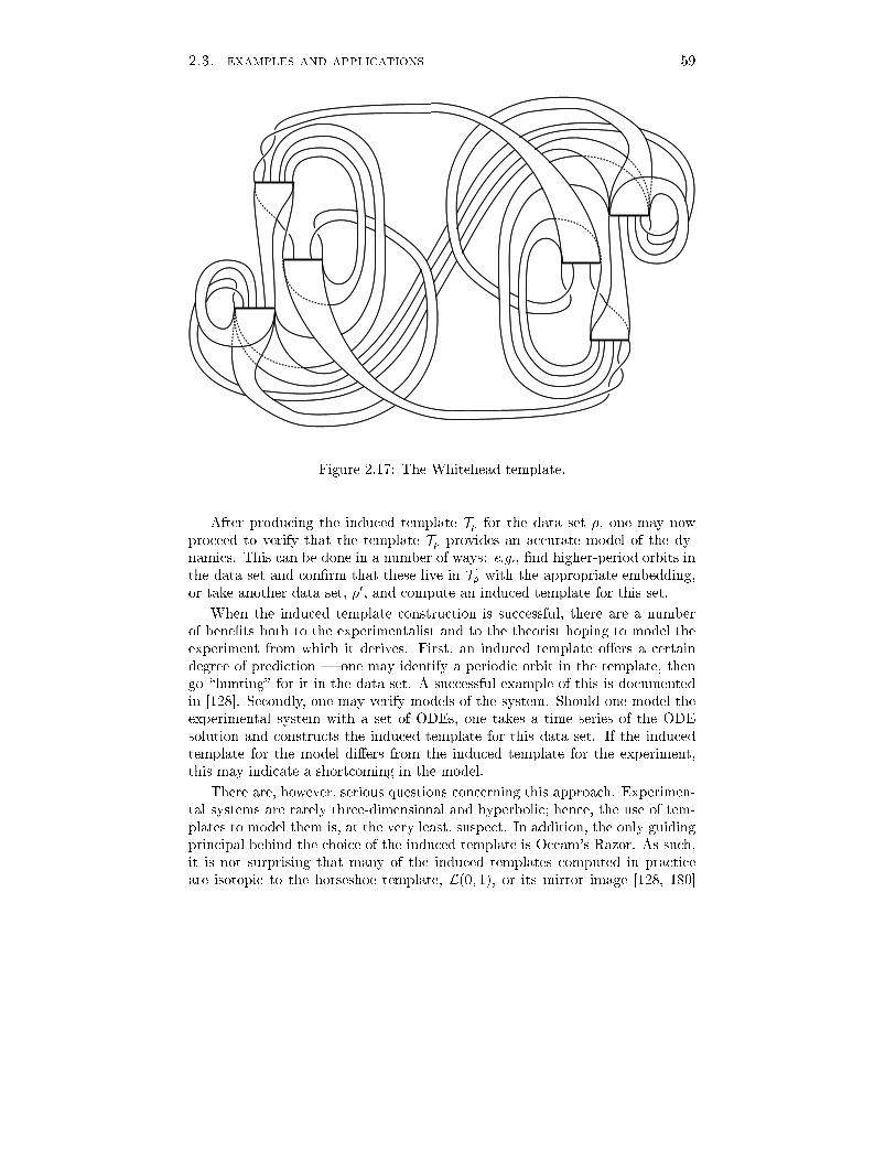
2.3. examples and applications 59

Figure 2.17: The Whitehead template.After producing the induced template T� for the data set �, one may nowproceed to verify that the template T� provides an accurate model of the dy-namics. This can be done in a number of ways: e.g., �nd higher-period orbits inthe data set and con�rm that these live in T� with the appropriate embedding,or take another data set, �0, and compute an induced template for this set.When the induced template construction is successful, there are a numberof bene�ts both to the experimentalist and to the theorist hoping to model theexperiment from which it derives. First, an induced template o�ers a certaindegree of prediction | one may identify a periodic orbit in the template, thengo \hunting" for it in the data set. A successful example of this is documentedin [128]. Secondly, one may verify models of the system. Should one model theexperimental system with a set of ODEs, one takes a time series of the ODEsolution and constructs the induced template for this data set. If the inducedtemplate for the model di�ers from the induced template for the experiment,this may indicate a shortcoming in the model.There are, however, serious questions concerning this approach. Experimen-tal systems are rarely three-dimensional and hyperbolic; hence, the use of tem-plates to model them is, at the very least, suspect. In addition, the only guidingprincipal behind the choice of the induced template is Occam's Razor. As such,it is not surprising that many of the induced templates computed in practiceare isotopic to the horseshoe template, L(0; 1), or its mirror image [128, 180]

60 chapter 2. templates

Figure 2.18: A time series derived from the Lorenz equations.(though see [106] for an exception).These doubts notwithstanding, there are numerous open questions about theuse of induced templates for time series, whose answers could be of great valueto experimentalists and modelers of complicated dynamics.2.4 A symbolic languageMuch of this book is concerned with templates and the links they carry. Toanalyze these, it is often useful to extract subtemplates, or subsets which arethemselves templates (see De�nition 2.4.6). In the late eighties, one of us [MS]noticed that the template V , illustrated in Figure 2.21 below, contains a sub-template which is isotopic to itself: see Figure 2.22 (this was used to show theexistence of highly-composite knots on V [169]). In this section, we introduceconventions for symbolic descriptions of orbits and templates, which enables usto signi�cantly generalize this kind of procedure to cases in which direct visual-ization is not possible.2.4.1 Markov structures and symbolic coordinatesRecall from the proof of the Template Theorem in x2.2 that there is a naturalcorrespondence between orbits which remain on a template and one-sided symbol

2.4. a symbolic language 61sequences in a subshift of �nite type: in particular, following upon Remark 2.2.8,we haveLemma 2.4.1 Given a template T , label the strips fxi : i = 1::Ng. Let AT bean N�N matrix with entry AT (i; j) = 1 if the incoming portion of xi meets theoutgoing portion of xj at a branch line, zero otherwise. Then �T , the set of allforward orbits which remain on T , is precisely the set of admissible sequences inthe subshift of �nite type given by AT .Proof: See the proof of Theorem 2.2.4, or simply collapse T along the transversedirection of the semi ow, reducing T to an oriented graph. Then the orbits onT are one-sided directed paths on this graph: cf. Remark 1.2.22. 2The way in which orbits �t together on a template T is described by placinga coordinate system on the branch lines f`j : j = 1::Mg, following the kneadingtheory of x1.2.3, and specifying the induced coordinates on �T . This orderingof orbits on a template is a key ingredient in discerning the relative placementof orbits on a template which might be too complicated to visualize.De�nition 2.4.2 Let T be a template with strips labeled fxigN1 . Denote byf`jgM1 the branch lines of T (one for each branch line chart). Then �T ispartitioned into N branch segments, denoted f�i(T )gN1 , where�i(T ) � fa = a0a1a2 : : : 2 �T : a0 = xig : (2.17)Denote by �`j � �T the union of �i(T ) over all i such that the strip xi emanatesfrom the branch line `j . We will sometimes refer to the union of the �i(T ) asthe branch set, denoted �(T ).Proposition 2.4.3 There exists a total ordering � on each �`j which respectsthe topology of �`j : that is, if a�b and fang is a sequence converging to a then,for suÆciently large n, an�b.Proof: This follows from the kneading theory [125], as outlined in x1.2.3. Weconstruct � explicitly in what follows, and it will be seen to have the followingproperty: � is the total ordering induced by the one-dimensionality of `j . Thatis, any point of an `j is an orbit which \begins" on `j . Orienting `j yields a totalorder on �`j which respects the topology. 2For the moment, assume T is an orientable template. Each branch line `j isone-dimensional. Hence, the set of branch segments in each `j are ordered (upto orientation of `j). If, for example, the branch segments x1; x2; : : : ; xp lie in `1in this order, then choose � as eitherx1 � x2 � : : :� xp; or xp � : : :� x2 � x1: (2.18)Having chosen an orientation for each `j , one then orders each �`j lexicograph-ically with respect to the ordering on the generators fxig. That is, given a andb 2 �`j , let J equal the index of the �rst symbol in which a and b disagree:J = min fj : aj 6= bjg : (2.19)

62 chapter 2. templatesThen a�b if aJ�bJ , else b�a. Of course, one cannot compare points in di�erent�`j : there is no notion of orientation for points on disjoint branch lines. SinceT is orientable, the lexicographical ordering of itineraries corresponds to theordering on the branch lines and it yields a natural coordinate system.For nonorientable templates, the issue is no more diÆcult, but it does demandmore bookkeeping. If a particular strip, say xj , contains an odd number of half-twists (i.e., the return map is orientation reversing on that interval), then onemust keep track of the parity of that symbol in using � as in the invariantcoordinate construction for the one-dimensional map fT of x1.2.3.Speci�cally, given a nonorientable template T , construct a provisional order-ing ~� as for an orientable template induced by the ordering on the individualbranch lines (as above). This ordering ~� does not, however give an orderingon T which respects the topology of the branch lines. Now, given some pla-nar presentation of T (a pictorial representation in which all the branch lineslie within the plane), each strip xi will have �(xi) half-twists for some signedinteger �(xi). Partition the strips fxig according to those which are orientationpreserving (�(xi) even) and those which are orientation reversing (�(xi) odd).Note that this partition depends on the choice of planar representation, and, inpractice, one wants to choose as simple a presentation as possible. Given pointsa and b in �`j , de�ne J as in Equation (2.19), and consider the parity � 2 f0; 1gwhich keeps track of orientation� � J�1Xi=0 �(ai)! mod 2: (2.20)Then de�ne the ordering � on �`j in terms of the provisional ordering ~� by� = 0 : a� b, a~�b� = 1 : b� a, a~�b:This ordering � re ects the \physical" ordering of orbits on the nonorientabletemplate T . It is clear that this procedure can be easily implemented on acomputer.Equipped with the ordering �, we can treat �T as being embedded in a�nite disjoint union of one-dimensional segments (although �T is really a Cantorset). As such, we will introduce some notation for branch segments. Recall fromDe�nition 2.4.2 that �T partitions intoN branch segments, where �i(T ) denotesall itineraries beginning with xi. Since this geometrically represents all orbitswhich begin at the xi-strip, we will consider �i(T ) as a closed interval, re ectingthe total ordering �:De�nition 2.4.4 Given T a template with strips fxigN1 and branch set �(T ),let the ith-left-boundary, @i (T ), be the point of �i(T ) which is �-minimal. Sim-ilarly, let the ith-right-boundary, @ri (T ) , be the point of �i(T ) which is �-maximal. The boundary set, @(T ), is given as the union of f@i (T ); @ri (T )g overi.

2.4. a symbolic language 63It is clear that @(T ) consists of the 2N eventually periodic orbits which togethercomprise the boundary of the template.Remark 2.4.5 In ows whose templates have a single branch line, correspond-ing to a global cross section, it is natural to identify the period of a closed orbitwith the number of intersections with the branch line. Often, this coincideswith the number of strands in a closed braid representation. In the more generalcontext of the present work, we identify the period of an orbit with the numberof intersections of the orbit with all branch lines (hence, the period of the orbitfor the return map induced by the branch lines). In all cases it coincides withthe length of the periodically repeating block in the corresponding orbit word.We will thus sometimes refer to this block length as the symbolic period.For a given template T , the symbolic data; �T ; AT ; �(T ); @(T ), and �,encode the dynamics and the combinatorial structure of the template. They donot, however, specify the topology of the enclosed orbits, nor do they provideinvariants of the underlying link LT , since one may change the embedding ofT without altering the symbolic data. Conversely, we may re�ne the Markovpartition (i.e., increase the number of branch segments) without discarding anyorbits from the template: see Figure 2.19 for an example. Even so, these symbolictools do become useful in describing proper in�nite sublinks and in describingthe relative placement of complicated orbits.Figure 2.19: Two templates which carry the same dynamics and topology onthe periodic orbits, but which have di�erent symbolic structures.2.4.2 Subtemplates and template in ationsIn the study of templates and their properties, there are varying \scales" at whichone may choose to work. Often, the knowledge of which types of individual knotsor links appear on a given template is useful: this is a \small scale" question.For example, in x4.2, we will see how careful bounds on the genus of individualhorseshoe knots can be used to derive uniqueness and bifurcation results in afamily of H�enon maps. On the other hand, one might ask \large scale" questionsabout whether two entire templates (including all their orbits) are equivalent.This perspective will come into play in Chapter 5. Here, however, we focus on

64 chapter 2. templatesa \medium" scale question: we examine subsets of orbits which are proper yetnon-�nite. These are described via the notion of subtemplates.De�nitions and examplesDe�nition 2.4.6 A subtemplate S of a template T , written S � T , is a topo-logical subset of T which, equipped with the restriction of the semi ow of T toS, satis�es the de�nition of a template (De�nition 2.2.1).A subtemplate is thus a compact branched submanifold with boundary, for whichthe original semi ow restricts to an expanding semi ow.Example 2.4.7 An example of a subtemplate of the Lorenz template is givenin Figure 2.20. When we \cut" along the boundaries of the subtemplate S �L(0; 0), we can remove S and isotope it into the nice presentation of Fig-ure 2.20(c). The move from part (b) to part (c) is one that we will encounteroften in the remainder of this work: it is the so-called belt trick, in which a curlis exchanged for a full twist.(a) (b)

(c)Figure 2.20: (a) a subtemplate S within L(0; 0), (b) when removed from L(0; 0),(c) is isotopic to L(0; 2).Note that S is a very special subtemplate of L(0; 0) in that S is di�eomorphicto L(0; 0) (it is in fact isotopic to L(0; 2) | recall Figure 2.8(a)). Although thisis not always the case, a di�eomorphic relationship between a template and asubtemplate opens up a new set of objects.De�nition 2.4.8 A template renormalization of a template T is a smooth em-bedding R : T ,! T which respects orbits (i.e., it commutes with the semi ow).

2.4. a symbolic language 65It follows from De�nition 2.4.6 that the image of a template renormalizationR(T ) is a subtemplate of T which is di�eomorphic to T . Returning to Example2.4.7, the subtemplate S � L(0; 0) is the image of a template renormalizationR : L(0; 0) ,! L(0; 0).The terminology for De�nition 2.4.8 arises from the one-dimensional returnmaps for a template induced by the branch lines [47]. The image of a templaterenormalization is merely a renormalization of the return maps, suspended inaccordance with the template structure. We prefer, however, to think in terms ofrenormalizing the branched two-manifold itself, since template renormalizationscarry with them the topology of the periodic orbits as well.Since a template renormalization R acts on orbits of T di�eomorphically, Rmaps periodic orbits to periodic orbits: hence, there is a topological action on theunderlying link LT . When this action is trivial, we say that the renormalizationis isotopic.De�nition 2.4.9 Let R : T ,! T be a renormalization on an embedded tem-plate T � S3 and let iT denote the inclusion of T into S3. If iT and iT ÆR areisotopic embeddings of T in S3, then R is an isotopic renormalization.The existence of a template renormalization immediately allows one to iterateR on the renormalized subtemplate. This procedure enables one to extract very\deep" subtemplates, which may contain signi�cant information about the peri-odic orbit link. When the renormalization has trivial action on the topology ofthe underlying periodic orbit link, we may iterate to obtain complicated subtem-plates whose orbits have extremely long symbolic period, while still controllingthe individual knot and link types.x1 x2x3 x4Figure 2.21: The template V .Example 2.4.10 The �rst example of an isotopic template renormalization(without that terminology) was given by M. Sullivan [169]. Let V denote the

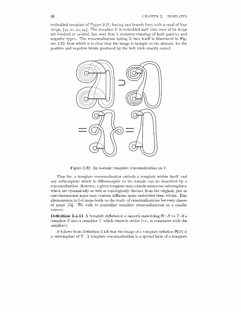
66 chapter 2. templatesembedded template of Figure 2.21, having two branch lines with a total of fourstrips, fx1; x2; x3; x4g. The template V is embedded such that none of its stripsare knotted or twisted, but note that it contains crossings of both positive andnegative types. The renormalization taking V into itself is illustrated in Fig-ure 2.22, from which it is clear that the image is isotopic to the domain, for thepositive and negative twists produced by the belt trick exactly cancel.

Figure 2.22: An isotopic template renormalization on V .Thus far, a template renormalization embeds a template within itself, andany subtemplate which is di�eomorphic to its domain can be described by arenormalization. However, a given template may contain numerous subtemplateswhich are dynamically as well as topologically distinct from the original, just asone-dimensional maps may contain di�erent maps embedded deep within. Thisphenomenon in 1-d maps leads to the study of renormalizations between classesof maps [73]. We wish to generalize template renormalizations in a similarmanner.De�nition 2.4.11 A template in ation is a smooth embedding R : S ,! T of atemplate S into a template T which respects orbits (i.e., it commutes with thesemi ow).It follows from De�nition 2.4.6 that the image of a template in ation R(S) isa subtemplate of T . A template renormalization is a special form of a template

2.4. a symbolic language 67in ation, and we will often use the more general term. The analogous notion ofan isotopic template in ation follows:De�nition 2.4.12 Let R : S ,! T be an in ation of a template S � S3 into atemplate T � S3. Let iS and iT denote inclusion of S and T respectively intoS3. If iS and iT ÆR are isotopic embeddings of S in S3, then R is an isotopicin ation.There are many basic questions about subtemplates and template in ations,e.g.:Problem 2.4.13 Given a template T , which templates embed [abstractly] inT (i.e., which are images of in ations)? Given an embedded template T , whatare all the subtemplates of T (i.e., which are images of isotopic in ations)?We will obtain in x3.3 the surprising answer that all orientable templates em-bed in any T (after a slight perturbation at the branch lines). Furthermore,we will show that certain templates contain isotopic copies of all templates assubtemplates.The goal of working with template in ations is to understand properties ofdeep, complicated subtemplates within a given template. To that end, isotopicin ations are useful, in that we can keep track of the knots and links whichlive \deep within" a template by pulling back the isotopy. To keep track ofwhere exactly these complicated subtemplates lie, we use the induced actionof an in ation on the itinerary space in order to derive \coordinates" for asubtemplate associated to a given in ation.Symbolic actions of in ationsLemma 2.4.14 A template in ation R : S ,! T induces an embedding R :�S ,! �T whose action is to in ate each symbol fxi : i = 1::Mg of �S to a�nite admissible word fwi = w1 : : : wn(i) : i = 1::Ng in the symbols of �T .Proof: by De�nition 2.4.11, R maps the branch lines of S into branch lines ofT . Hence, each strip of S (corresponding to a generator xi of �S) is mapped toa �nite sequence of strips in T , corresponding to a �nite admissible itinerary forT . 2The image under R of any orbit on S is thus obtained by \in ating" eachsymbol xi in the itinerary by the word wi (which in some cases may consist ofa single letter). This immediately implies the following useful result:Corollary 2.4.15 Given R : S ,! T a template in ation, the branch set andthe boundary of the subtemplate R(S) are given by�i(R(S)) = R(�i(S)) = fR(a); a 2 �i(S)g@(R(S)) = R(@(S)) = fR(a); a 2 @(S)g : (2.21)

68 chapter 2. templatesWe wish to consider the branch set �(R(S)) as a set of \coordinates" consistingof N \subintervals" of the branch set of T which indicate where S resides withinT . We note that the image of a branch segment under an in ation is not aninterval in the sense that all orbits between its endpoints are not necessarilypart of the subtemplate (recall there are \gaps" in the branch lines). Yet, if weconsider the N subintervals given by �(R(S)), we have a relative measure of thedepth of an in ation. For example, if a template T contains a nested sequenceof subtemplates Tn � : : : � T2 � T1 � T , then the same inclusion exists on thebranch sets �(Ti) within �(T ). Or, given two subtemplates of T , the informationencoded in their symbolic branch sets can be used to determine whether thesesubtemplates are disjoint, or which subtemplate is \closer" (under �) to a givenperiodic orbit.Example 2.4.16 For an example which will demonstrate the symbolic actionsof an isotopic in ation, we return to the isotopic renormalization of V fromExample 2.4.10. From Figure 2.22, one traces the image of the four stripsfx1; x2; x3; x4g to obtain the symbolic action:D : V ,! V 8>><>>: x1 7! x1x2 7! x1x2x3 7! x3x4 7! x3x4 : (2.22)The branch segments of the subtemplate are given by�1(D(V)) = D ([(x1)1 ; x1 (x2x4)1]) = [(x1)1 ; x1 (x1x2x3x4)1]�2(D(V)) = D ([x2 (x3)1 ; (x2x4)1]) = [x1x2 (x3)1 ; (x1x2x3x4)1]�3(D(V)) = D ([(x3)1 ; x3 (x4x2)1]) = [(x3)1 ; x3 (x3x4x1x2)1] (2.23)�4(D(V)) = D ([x4 (x1)1 ; (x4x2)1]) = [x3x4 (x1)1 ; (x3x4x1x2)1] :The boundary components of the subtemplate, @(D(V)), are given by the end-points of the intervals above.We encourage the reader to work through this example carefully, correlatingthe geometric description of Figure 2.22 with the symbolic description of Equa-tion (2.22). This procedure is used extensively in Chapter 3.Unfortunately, one cannot endow the symbolic structure with very muchinformation about the topology of the in�nite link. However, the hyperbolicityof the underlying ow does give a nice structure to the space �T which we hopeto utilize as much as possible. By looking at the ordering � and by consideringthe relationship between iterated subtemplates and their \coordinates" in termsof branch sets, we have a set of tools for describing and manipulating \deep"sublinks of the link of periodic orbits. We will use these in the next chapter toprove some basic, as well as some surprising, results.

Chapter 3: Template TheoryIn this chapter, we use the tools of Chapter 2 to build a collection of generalresults on templates and template links, noting applications to the dynamicsof three-dimensional ows along the way. We begin in x3.1 with a treatmentof properties of the individual knots and links which are supported on a givenembedded template. Then, in x3.2, we use the methods developed in x3.1 and theprevious chapter to prove the existence (and abundance) of universal templates:templates which contain all knots and links among their closed orbits. Inx3.3, we continue this line of inquiry to examine the subtemplate problem: theenumeration of all subtemplates of a given embedded template.These results, which are fairly general in nature, will lead to numerous speci�cconclusions in this and in subsequent chapters when applied to the examplesintroduced in x2.3.3.1 Knotted orbits on templatesQuestion 1 Given an embedded template T , does it contain a nontrivial knot?How many such knots are present? How are these distributed?In this section, we will answer Question 1, giving applications to the dynamicsof ows.3.1.1 Alexander's Theorem for templatesIn many of the results to follow, we will need to represent template knots andlinks as closed braids. We begin with an analogue of braiding for templates:De�nition 3.1.1 A template T is said to be braided if T is embedded inD2�S1in such a way that every closed orbit on T is a closed braid: that is, eachmeridional disc D2 � f�g intersects the curve transversely in a �xed number ofpoints. A template is said to be positive if it can be braided in such a way thatevery closed orbit is a closed positive braid.Recall Alexander's Theorem (Theorem 1.1.13), which states that any link isisotopic to a closed braid. The corresponding statement for templates is alsotrue, as shown by Franks and Williams [58].Theorem 3.1.2 (The Alexander Template Theorem: Franks andWilliams[58]) Any template T may be isotoped so that it is a closed braided template.Furthermore, if T is orientable, it may be arranged such that in a planar pro-jection, all the strips of T are at (untwisted).69

70 chapter 3. template theoryThe proof closely follows that of Alexander's Theorem for links [3]: a nice accountof the latter can be found in [33, Prop. 2.14]. In the proof of Alexander'sTheorem, one chooses a tenative braid axis, and then iteratively \ ips" strandsof the link about the braid axis until they are all aligned. Here, instead ofwrapping strands about a braid axis, one manipulates strips. To obtain a atpresentation, one uses the belt trick of Example 2.4.7 to exchange a full twist foran additional trip about the braid axis. Half twists, which arise in non-orientabletemplates, of course cannot be straightened.3.1.2 Concatenation of template knotsGiven two periodic points of �`j { the set of all orbits starting on the branchline `j { we wish to de�ne an \addition" operation which has both symbolic andtopological interpretations.De�nition 3.1.3 Let a1 and b1 be distinct periodic points of �`j . Then theconcatenation of a1 and b1, denoted a1 � b1, is the point (ab)1 2 �`j .Remark 3.1.4 The concatenation operation is well-de�ned: since a1 and b1are both points on a particular branch line `j , the orbit (ab)1 must be admis-sible. Note, however, that ab may equal uk for k > 1 and some u, as in x21x2x1concatenated with x1x2. In this case, we would say �x21x2x1�1 � (x1x2)1 =�x21x2�1.Given the concatenation operation, we wish to understand the topological actionon periodic orbits. We begin with a class of concatenations which behave nicely.De�nition 3.1.5 Choose two distinct points u and v 2 �`j and assume thatu�v. De�ne (u;v) to be the set of all point x 2 �`j such that u�x�v. Thenu and v are said to be adjacent if,��kuk>0 \ (u;v) = ��kvk>0 \ (u;v) = ;: (3.1)Thus, u and v are adjacent if no other points on their orbits appear between uand v.In order to simplify the next few results, we circumvent the exceptional casesof Remark 3.1.4:Lemma 3.1.6 If a and b are distinct nontrivial words and ab = uk for k > 1and some u, then a1 and b1 are not adjacent.Proof: Decompose a = uia0 and b = b0uj , where i + j = k � 1 and a0b0 = u.Assuming (arbitrarily) that a�b and that i > 0, consider the point �ui�1a0u�1,which is a shift of a1. Then, since a1 � u1 � b1, it follows thata1 � �ui�1a0u�1 � u1 � b1; (3.2)whence it follows that a1 and b1 are not adjacent. 2The concatenation of adjacent orbits is similar in spirit to taking a connectedsum: only one crossing is added.

3.1. knotted orbits on templates 71Lemma 3.1.7 Let T be an embedded template, and let a1 and b1 be adjacentperiodic points in �`j . The planar presentation of the knot corresponding toa1 � b1 di�ers from that of the link corresponding to a1 union b1 by theaddition of a single crossing (as illustrated in Figure 3.1).Proof: Place T in a planar presentation and consider the branch line `j whichcontains the points a1�b1. By isotoping T if necessary, a neighborhood of `jwill appear locally as in Figure 3.1(a) { there are two cases depending on whichstrip is \on top." By properties of the ordering �, it follows thata1 � (ab)1 � (ba)1 � b1; (3.3)so that the concatenated orbit appears as in Figure 3.1(b): there is a new crossingwhose sign is dependent upon the stacking order of strips. The orbit (ab)1follows a then b: the ordering of points on other branch lines does not change.More speci�cally, if, on any branch line, ��ia�1 � ��ja�1, then it follows that��i(ab)�1 � ��j(ab)�1 for any i; j < jaj. Hence, a1 � b1 may be isotopedto the link a1 union b1 with a single crossing inserted at the branch line asspeci�ed. 2a1 b1 (ba)1(ab)1a1 b1 (ba)1(ab)1(a) (b)Figure 3.1: Concatenation of adjacent periodic points e�ects a local change asabove.Lemma 3.1.7 immediately yields:

72 chapter 3. template theoryCorollary 3.1.8 Let T be an embedded template, and let a1 and b1 be ad-jacent periodic points in �`j with self-crossing numbers ca and cb respectively.Then, the self-crossing number of the concatenation a1 � b1 is given byca�b = ca + cb + 2`k (a1;b1) + �; (3.4)where � = �1, depending upon a1;b1; and T , is the sign of the crossing ofLemma 3.1.7.De�nition 3.1.9 The twist of a ribbon (annulus or M�obius strip) in S3 withc crossings and t signed half-twists (in a given planar presentation) is given asc + 12 t and is an isotopy invariant (see Lemma 5.3.4 for a proof). Given K aclosed orbit on a template T , the twist of K, �K , is de�ned to be the twist of thenormal bundle of T restricted to K. That is, the bundle of normal directions toT along K is an embedded ribbon in S3 with twist �K . Equivalently, this ribbonis the local stable manifold to the orbit.Corollary 3.1.10 Let T be an embedded template, and let a1 and b1 be adja-cent periodic points in �`j . Then the twist of the concatenated knot correspondingto the point a1 � b1 is given by�(a1 � b1) = �(a1) + �(b1) + 2`k (a1;b1) + �; (3.5)where � = �1; depending upon a;b, and T .Proof: Apply Lemma 3.1.7 to De�nition 3.1.9. 2Corollary 3.1.11 Let T be an embedded positive template, and let a1 and b1be adjacent periodic points in �`j for some j. Then the genus of the concatenatedknot corresponding to the point a1 � b1 is bounded below asg(a1 � b1) � g(a1) + g(b1): (3.6)Proof: Arrange T as a braided template with all crossings positive. Via Equation(1.3), the genera of the knots corresponding to a1 and b1 are, respectively,g(a1) = ca �Na + 12 ; g(b1) = cb �Nb + 12 ; (3.7)where c denotes number of crossings and N denotes number of strands. Theconcatenated knot a1 � b1 has Na +Nb strands in its braid presentation, andit has crossing number given by Equation (3.4). Thus,g(a1 � b1) = ca + cb + 2`k (a1;b1) + �� (Na +Nb) + 12= g(a1) + g(b1) + 2`k (a1;b1)� 1 + �2 : (3.8)

3.1. knotted orbits on templates 73Since all crossings are positive prior to and after concatenation, `k (a1;b1) � 0.If � = �1, then in concatenation we have removed a (positive) crossing; thus,for � = �1, `k (a1;b1) > 0 prior to concatenation, and the result follows. For� = +1, it is obviously true. 2Corollary 3.1.11 gives a partial answer to a generalization of a conjecture ofWilliams's:Conjecture 3.1.12 Let T be a positive embedded template. Let a1 and b1 beperiodic itineraries in �`j (not necessarily adjacent). Then, genus is monotonicunder the � operation:1 g((ab)1) � g(a1) + g(b1): (3.9)We will use the � operation in the next subsection, when we describe where ona template knots live.3.1.3 The existence of knots on a templateTheorem 3.1.13 Given an embedded template T , there exists a nontrivial knotas an orbit on T .Proof: Our proof is in the spirit of Proposition 4.4 of [58], in that we rely uponthe Bennequin inequality.2 Arrange T as a braided template as per Theorem3.1.2. Choose a1 and b1 in some branch set component �`j with a1 and b1adjacent. Assume that the twist of a1 or b1 is nonzero. If not, then replacea1 with a1 � b1. By Corollary 3.1.10, the twist of the concatenated knot isnonzero and this orbit is still adjacent to b1.Given a1 and b1 with �(a1) 6= 0, concatenate repeatedly to form the orbit(anb)1 = a1 � (a1 � (� � � (a1 � b1) � � �)): (3.10)We will use the Bennequin inequality, Equation (1.5), to bound the genus of thisknot. By Corollary 3.1.8, the self-crossing number of (anb)1 iscanb = can2 + 12 tan(n� 1) + cb + (2`k (a1;b1) + �)n; (3.11)where ca (resp. cb) is the self-crossing number of a1 (resp. b1), ta is the signednumber of half-twists in the presentation of the embedded normal bundle of a1,and � = �1. See Figure 3.2 for the count of the terms quadratic in n. ByEquation (1.5),2g((anb)1) � ��can2 + 12 tan(n� 1) + cb + (2`k (a1;b1) + �)n���(nNa +Nb) + 1 ; (3.12)1An exception occurs as in Remark 3.1.4, which we could circumvent by de�ning the genusof �uk�1 to be k times the genus of u1.2It is an open (and challenging) problem to prove this theorem without resorting to Ben-nequin's inequality.

74 chapter 3. template theorySince the twist �a 6= 0, ca + 12 ta 6= 0; hence, canb is quadratic in n as per (3.11).Thus, for some n, the genus of (anb)1 is nonzero. 2k k j(a) (b)Figure 3.2: (a) each half-twist on k-strands yields 12k(k � 1) crossings; (b) eachcrossing of k-strands over j-strands yields kj crossings.Corollary 3.1.14 Given an embedded template T , there exists an in�nite num-ber of distinct knot types as orbits on T .Proof: Let n!1 above. 2From this, we may recover the Franks-Williams Theorem for ows on S3:Theorem 3.1.15 (Franks and Williams [58]) Any C2- ow on S3 which haspositive topological entropy must display an in�nite number of distinct knot typesas closed orbits.Proof: By a [deep] theorem of Katok [97], a C2 ow with positive topologicalentropy must contain a hyperbolic periodic orbit which has a transverse homo-clinic connection. The Poincar�e-Birkho�-Smale Theorem, Theorem 1.2.33, thenasserts the existence of an embedded Smale horseshoe in the ow. By the Tem-plate Theorem, this basic set collapses to an embedded template in S3 whichcaptures knot and link types. This template, and hence the ow, supports anin�nite number of knot types by Corollary 3.1.14. 2Remark 3.1.16 Theorem 3.1.15 is a beautiful result, yielding a great deal oftopological information from purely dynamical data. The connection is thusestablished: dynamically complicated hyperbolic ows on S3 force topologicallycomplicated knots as orbits. Several converses exist: for an example, see the

3.1. knotted orbits on templates 75Morgan-Wada Theorem in Appendix A. Another well-known converse is theSeifert Conjecture, recently resolved in the smooth case by K. Kuperberg [107].This result states that there exist smooth nonsingular ows on S3 containing noperiodic orbits whatsoever.From Theorem 3.1.13 we may also derive information about how knots aredistributed on �T . We show that the nontrivial knots do not con�ne themselvesto any proper subregion.Corollary 3.1.17 Let T be an irreducible template | that is, the subshift of�nite type de�ned on �T has a dense orbit. Then, given any point x in �T , thereexists an in�nite number of distinct knot types represented in an arbitrarily smallneighborhood of x.Proof: Choose a small �-neighborhood N� of x in �T and pick two distinctperiodic points a1 and b1 2 N� (this is always possible since the periodicpoints are dense in �T for T irreducible). If necessary, shift b1 to be adjacentto a1 | this does not remove it from N�. Consider the template in ationR : L(�a; �b) ,! T � x1 7! ax2 7! b ; (3.13)where �a (�b resp.) is the twist of a1 (b1 resp.) and L(m;n) is the Lorenz-liketemplate of type (m;n) (see x2.3.1). This in ation is well-de�ned since a1 andb1 are adjacent. The image of R has branch set�fR(L(�a; �b))g = 8<: [a1;b1] : �a; �b even[a1;ba1] : �a even ; �b odd[ab1;ba1] : �a; �b odd ; (3.14)which is contained within a 2�-neighborhood of a1. By Corollary 3.1.14, thissubtemplate contains an in�nite set of distinct knot types. 2Remark 3.1.18 Any template obtained from a basic set of a ow is irreducible,since basic sets have dense orbits. A non-irreducible template is, from our per-spective, an anomaly.3.1.4 Accumulations of knotsKnowing that knot types are \densely packed" on any given template says noth-ing about their precise distribution. What are the chances of a �gure-eight knotliving arbitrarily close to a trefoil? To an unknot? To answer this (in part), wewill explore the special role played by unknots with zero twist.Proposition 3.1.19 Let T be an embedded template. Suppose that some pointu1 2 �`j represents an unknotted periodic orbit with zero twist. Then, forevery periodic point a1 in �`j such that a1 and u1 are separable, there existin�nitely many periodic points in �`j which have the same knot type as a1, andthese accumulate onto u1.

76 chapter 3. template theoryProof: Assume (after shifting perhaps) that a1 and u1 are adjacent. We claimthat the concatenation u1 � a1 = (ua)1 is the connected sum of the twooriginal knots.Since a1 and u1 represent separable knots, there is a 2-sphere S2 whichbounds the knots on opposite sides. By placing the sphere in general position,we may assume that S2 intersects the template T transversally. Denote by Ithe subset of the branch line `j which is bounded by the points u1 and a1.Let N � S3 denote a tubular neighborhood of u1 [ I [ a1 in S3. Weclaim that N \ T is isotopic to the con�guration of Figure 3.3. To show this,note that the space S3 n N is isotopic to a solid torus (the complement of theunknot u1) with an interior solid torus removed (a neighborhood of the knota1) and a (perhaps knotted) hole connecting the boundaries of these solid tori,corresponding to the arc I . Since a1 and u1 are separable, the solid torus holein inessential (it is contained within a ball in the solid torus). As such, one mayuse the \lightbulb trick" | if a lightbulb hangs from a knotted cord, the cordcan be isotoped to one without a knot while �xing the light bulb | to show thatN can be isotoped to the con�guration of Figure 3.3 (see [154, p. 257]).

Figure 3.3: The intersection of N and T .Given N \T as in Figure 3.3(a), the orbit (ua)1 is isotopic within T (hence,within S3) to a curve within N . This isotopy involves pushing the orbit \out-wards" so that it completes a circuit in a neighborhood of a1, crosses to b1through I , continues around b1, then goes back across I .After the isotopy, it is clear that (ua)1 is the connected sum of u1 and a1.Since u1 is an unknot, (ua)1 has the knot type of a1. Since u1 is unknottedand untwisted, (ua)1 is also separable with respect to u1 and the process maybe iterated, creating the sequence �uka�1, which accumulates on u1. 2A converse to Proposition 3.1.19 holds for positive templates and provides aclue to the distribution of knots on templates.Theorem 3.1.20 Let T be a positive embedded template. Suppose that a se-quence of distinct periodic points a1n in �T all correspond to the same knot

3.1. knotted orbits on templates 77type. Then any accumulation point of this sequence of the form u1 representsan untwisted unknotted periodic orbit.Proof: Arrange T as a positively braided template as per Theorem 3.1.2. Givenu1 an accumulation point for the sequence a1n , reindex this latter sequence todenote the subsequence which converges to u1. For n suÆciently large, a1n mustbe of the form �ukbn�1 for k any �xed number: this is pictured in Figure 3.4.If u1 is nontrivially knotted, then by Equation (1.3), cu > Nu, where cu isthe self-crossing number and Nu is the number of strands in the braid represen-tation of u1. From the form of a1n = �ukbn�1, it follows that the genus ofa1n is greater than or equal to k times the [nonzero] genus of u1. As k can bechosen arbitrarily large, the sequence fa1n gn will not have bounded genus.u1 a1

Figure 3.4: A portion of the orbit a1n for n large.If u1 is an unknot of twist �u > 0, then there are at least 12�uk(k� 1) cross-ings of a1n = �ukb�1 with u1 (cf. Figure 3.2). Since, for n large, k is large,Equation (3.8) implies that the genus of the sequence fa1n g is unbounded. Weconclude that u1 is an untwisted unknot. 2Theorem 3.1.20 implies that, on a positive template T , the collection of knottypes supported on T \accumulates" at untwisted unknots and nowhere else.Remark 3.1.21 Let f ig11 be a sequence of distinct closed orbits in a ow. Wesay that i accumulates on a closed orbit if there exists a sequence of pointsfxi 2 ig11 which have x 2 as an accumulation point for some x 2 . Ifwe consider the class of ows that have one-dimensional basic sets (e.g., Smale ows) with \positive" twisting, we can lift Theorem 3.1.20 to the original ow

78 chapter 3. template theoryto imply that any in�nite sequence of distinct periodic orbits of bounded genusmust accumulate on untwisted unknots.Remark 3.1.22 Theorem 3.1.20 fails spectacularly for non-positive templates.Using results from the remainder of this chapter, it has recently been shown thatin such cases, practically anything can occur: see Remark 3.3.12.3.2 Universal templatesWe have in Theorem 3.1.13 one extreme: every embedded template must containa nontrivial knot, and in fact, by Corollary 3.1.14, in�nitely many distinct knots.The other extreme, however, is unclear, as to whether an embedded template cancontain all knots. Certainly, the �gure-eight knot cannot live on the embeddedLorenz template L(0; 0), as this template is positive and the �gure-eight knotcannot be represented by a positive braid (recall Exercise 1.1.21). Hence, thereexist classes of templates which do not contain all knots.Question 2 Does there exist an embedded template T � S3 containing all knotsas periodic orbits? All links?The answer to Question 2 was conjectured to be no [24]: we will prove other-wise, outlining the arguments of [69], while providing a more general perspective.Question 2 is to some degree not the most general approach to understanding\what lives" in a given template. Focusing instead on the class of embeddedtemplates leads to the following question:Question 3 Given an embedded template T � S3, what are all the subtemplatesof T ?In this section, we tackle Question 2 by using methods suited for answeringQuestion 3.3.2.1 Examples of subtemplate structuresLorenz-like templatesAs a basic example of a subtemplate question, recall Problem 2.3.6 concerningthe relationships between the Lorenz-like templates of x2.3.1. We derive a partialanswer in this subsection, following [168], but using the symbolic methods of thismonograph.In Figure 2.20 of x2.4.2, we proved that L(0; 2) � L(0; 0) via an isotopicin ation. In the following, we use the symbolic descriptions of x2.4 to list aslightly more complete collection of isotopic in ations relating these templates.

3.2. universal templates 79Proposition 3.2.1 The following template in ations act isotopically:L(0; n+ 2) ,! L(0; n) � x1 7! x1x2 7! x1x2 (3.15)L(0;�2) ,! L(0;�1) � x1 7! x1x2 7! x22 : (3.16)Proof: For the �rst in ation, a simple generalization of Figure 2.20 is left to thereader. Figure 3.5 illustrates the isotopy for the second in ation. In both cases,one needs to use the belt trick when \pulling out" the subtemplate. 2Figure 3.5: The template L(0;�2) is a subtemplate of L(0;�1).The chain of inclusions among Lorenz-like templates implied by Proposition3.2.1 is� � � � L(0; 4) � L(0; 2) � L(0; 0) � L(0;�2) � L(0;�4) � � � �\� � � � L(0; 5) � L(0; 3) � L(0; 1) � L(0;�1) � L(0;�3) � � � � :(3.17)The templates U and VAs a more intricate example of subtemplate structures, we turn to two decep-tively simple templates �rst studied in [169] and later in [69].Let V denote the embedded template of Figure 3.6(a), also introduced inExample 2.4.10. Let U denote the embedded template of Figure 3.6(b). Eachtemplate has two branch lines, `1 and `2, and four strips, labeled x1; : : : ; x4.These templates are related in a fascinating way:Proposition 3.2.2 The following are isotopic template in ations:F : U ,! V 8>><>>: x1 7! x1x2 7! x1x2x3x3 7! x4x2x4 7! x4 ; (3.18)

80 chapter 3. template theoryx1 x2x3 x4

x1 x2x3x4(a) (b)Figure 3.6: (a) The template V ; (b) the template U .G : V ,! U 8>><>>: x1 7! x1x2 7! x1x3 7! x2x4x4 7! x2x3x4 : (3.19)Proof: See the isotopies in Figures 3.7 and 3.8. 2

Figure 3.7: The template in ation F acts isotopically.Proposition 3.2.2 presents a puzzling situation: U � V and V � U , and theinclusions occur in many di�erent ways. By incorporating the symbolic approachto subtemplates of x2.4, we can track these various inclusions. For example, Uand V display a symmetry which may be exploited to generalize the templatein ations F and G:

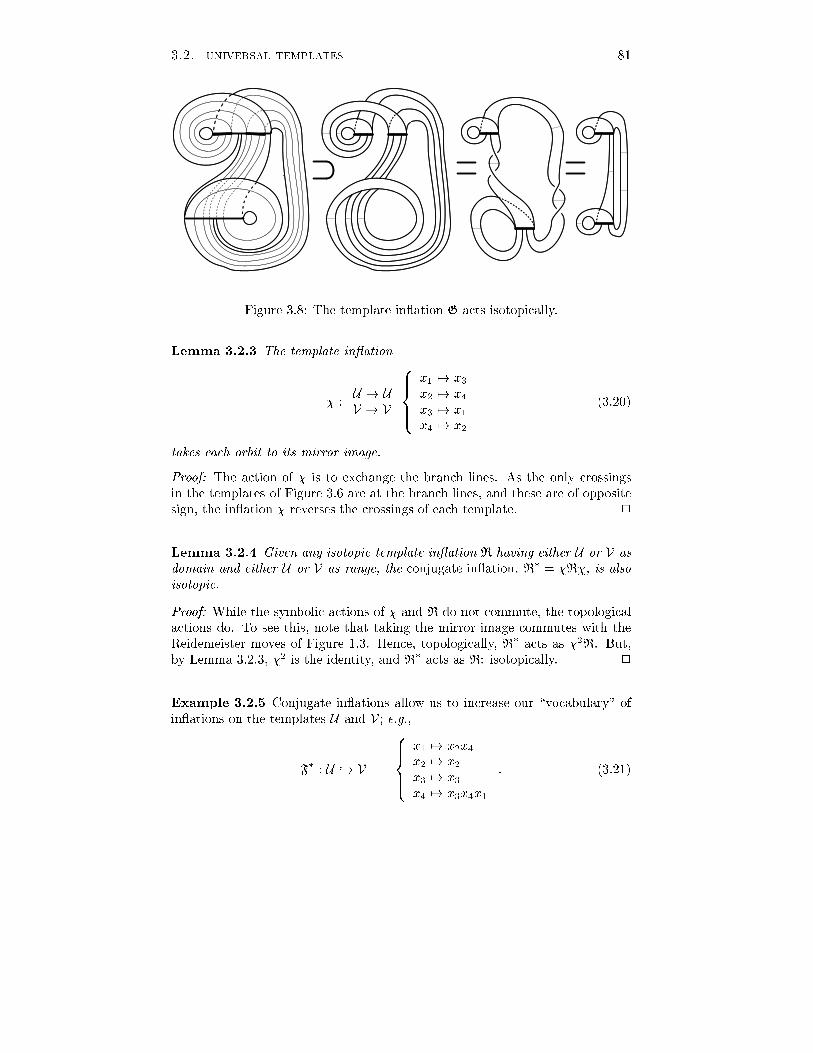
3.2. universal templates 81

Figure 3.8: The template in ation G acts isotopically.Lemma 3.2.3 The template in ation� : U ! UV ! V 8>><>>: x1 7! x3x2 7! x4x3 7! x1x4 7! x2 (3.20)takes each orbit to its mirror image.Proof: The action of � is to exchange the branch lines. As the only crossingsin the templates of Figure 3.6 are at the branch lines, and these are of oppositesign, the in ation � reverses the crossings of each template. 2Lemma 3.2.4 Given any isotopic template in ation R having either U or V asdomain and either U or V as range, the conjugate in ation, R� = �R�, is alsoisotopic.Proof: While the symbolic actions of � and R do not commute, the topologicalactions do. To see this, note that taking the mirror image commutes with theReidemeister moves of Figure 1.3. Hence, topologically, R� acts as �2R. But,by Lemma 3.2.3, �2 is the identity, and R� acts as R: isotopically. 2Example 3.2.5 Conjugate in ations allow us to increase our \vocabulary" ofin ations on the templates U and V ; e.g.,F� : U ,! V 8>><>>: x1 7! x2x4x2 7! x2x3 7! x3x4 7! x3x4x1 : (3.21)

82 chapter 3. template theoryComposing the simple in ations F and G with their conjugates yields a va-riety of interesting subtemplate structures: e.g.,Proposition 3.2.6 Let R : S ,! T be an isotopic in ation of some templateS into some template T . If R factors as R2GR1 for some isotopic in ationsR1 : S ,! V and R2 : U ,! T , then the image of the isotopic in ation R1G�R2is disjoint and separable from that of R.Proof: First, we isolate the action of the in ation G : V ,! U . Consider thesubtemplates given by the images of G and G�. The branch sets of these sub-templates are, due to Corollary 2.4.15,�(G(V)) = [x11 ; x1 (x1x2x3x4)1] [x1 (x2x4)1 ; (x1x2x3x4)1][(x2x4)1 ; x2x4 (x2x3x4x1)1] [x2x3x4x11 ; (x2x3x4x1)1]�(G�(V)) = [(x4x2)1 ; x4x2 (x4x1x2x3)1] [x4x1x2x13 ; (x4x1x2x3)1][x13 ; x3 (x3x4x1x2)1] [x3 (x4x2)1 ; (x3x4x1x2)1] :We claim that the images of these two in ations are disjoint subtemplates ofU , except for their common boundary orbit (x1x2x3x4)1. This may be shownby checking that certain shifts of �(G) (considered as \intervals" under �) donot intersect shifts of �(G�) except at their common boundary and at branchlines. Though this is perhaps computationally tedious, it is a �nite process whichworks when pictures fail.However, the simplest proof is to carefully check that Figure 3.9(a) accuratelyrepresents the subtemplates in question, and that these are disjoint. In Figure3.9(b), we crush out the transverse direction of the semi ow in each subtemplate,yielding a link of two graphs. From this, it is clear that these graphs, and hencethe subtemplates, are separable.It follows, then, that the images of R1GR2 and R1G�R2 must also be dis-joint and separable copies of S in T . 2Corollary 3.2.7 Each template U and V contains a countable in�nity of sub-templates isotopic to U and V which are completely disjoint and separable.Proof: De�ne the in ation An to be (FG) (FG�)n, for n = 0; 1; : : :. The imageof each An is a subtemplate of V isotopic to V thanks to Proposition 3.2.2. Weclaim that the image of An is disjoint and separable from the image of each An+kfor k > 0. To prove this, note that An+k factors asAn+k = nFG (FG�)k�1o (FG�)n+1 ; (3.22)so that the image of An+k is contained in the image of (FG�)n+1. By Proposi-tion 3.2.6, the images of An and (FG�)n+1 are disjoint and separable, since theydi�er by changing one G to G�. Therefore each template, V and U , containsin�nitely many separable copies of itself (and of the other template). 2

3.2. universal templates 83

Figure 3.9: The subtemplates G(V) and G�(V) (left) are disjoint and separable,as seen by reducing the subtemplates to embedded graphs (right).3.2.2 A template containing all linksThe embedded templates U and V of Corollary 3.2.7 entwine within one otherin surprisingly complicated ways. We will exploit these subtemplate webs toanswer basic questions about subtemplate structures. We begin with a solutionto the existence problem for templates which are \universal" in the class of links.Theorem 3.2.8 (Ghrist [69]) The embedded template V contains representa-tives of every �nite link as periodic orbits.The proof of Theorem 3.2.8 is the focal point of this chapter, and will beperformed in steps.We begin by examining a new family of templates, fWq ; q 2 Z+g, illustratedin Figure 3.10. Each Wq is an embedded q-fold cover of V ; that is, there are 2q\ears", or copies of the x1 and x3 strips. It is important to note that these earsalternate in crossing type | we denote them positive- and negative-type earsaccordingly.It is clear that there is a natural sequence of subtemplate inclusions V =W1 � W2 � W3 � : : : This increasing sequence is \large enough" to eventuallycontain any given link:Proposition 3.2.9 Given L an arbitrary link in S3, an isotopic copy of L ap-pears as a set of periodic orbits on the template Wq for q suÆciently large.Proof: Recall the braid group on N strands, BN , from x1.1, generated by theelements �i, i = 1:::N�1. We construct \local" representatives of each generator

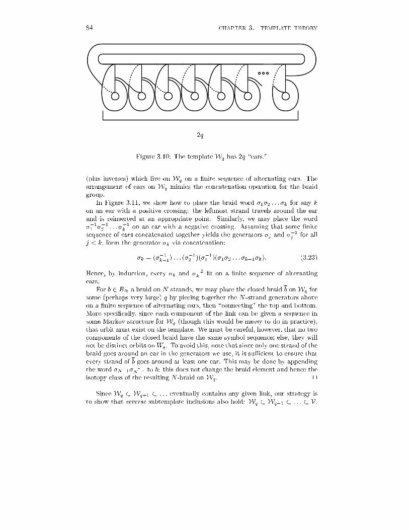
84 chapter 3. template theory

2qFigure 3.10: The template Wq has 2q \ears."(plus inverses) which live on Wq on a �nite sequence of alternating ears. Thearrangement of ears on Wq mimics the concatenation operation for the braidgroup.In Figure 3.11, we show how to place the braid word �1�2 : : : �k for any kon an ear with a positive crossing: the leftmost strand travels around the earand is reinserted at an appropriate point. Similarly, we may place the word��11 ��12 : : : ��1k on an ear with a negative crossing. Assuming that some �nitesequence of ears concatenated together yields the generators �j and ��1j for allj < k, form the generator �k via concatenation:�k = (��1k�1) : : : (��12 )(��11 )(�1�2 : : : �k�1�k): (3.23)Hence, by induction, every �k and ��1k �t on a �nite sequence of alternatingears.For b 2 BN a braid on N strands, we may place the closed braid b onWq forsome (perhaps very large) q by piecing together the N -strand generators aboveon a �nite sequence of alternating ears, then \connecting" the top and bottom.More speci�cally, since each component of the link can be given a sequence insome Markov structure for Wq (though this would be messy to do in practice),that orbit must exist on the template. We must be careful, however, that no twocomponents of the closed braid have the same symbol sequence; else, they willnot be distinct orbits onWq . To avoid this, note that since only one strand of thebraid goes around an ear in the generators we use, it is suÆcient to ensure thatevery strand of b goes around at least one ear. This may be done by appendingthe word �N�1��1N�1 to b: this does not change the braid element and hence theisotopy class of the resulting N -braid on Wq. 2Since Wq � Wq+1 � : : : eventually contains any given link, our strategy isto show that reverse subtemplate inclusions also hold: Wq � Wq�1 � : : : � V .

3.2. universal templates 85�1�2 : : : �k��11 ��12 : : : ��1k

Figure 3.11: The braid words �1�2 : : : �k and ��11 ��12 : : : ��1k �t on the ears ofWq .To �nd a copy of Wq within V , we develop a type of surgery for subtemplates ofV . We denote the following procedure appending an ear.Lemma 3.2.10 Let S � V be a subtemplate of V and let I = [@`(I); @r(I)] bethe component of S \ `1(V) which is minimal among all such intersections withrespect to the � ordering on the upper branch line. If @`(I) 6= x11 , then S iscontained in a subtemplate S+ � V and this template S+ is isotopic to S exceptfor the addition of an unknotted ear along I. Moreover, the subtemplate S+contains the orbit @4(V).Proof: The subtemplate S is completely determined by its branch set �(S), seeDe�nition 2.4.2. That is, given �(S), the subtemplate S is uniquely de�ned by owing each branch segment forwards until it completely covers a collection oftwo or more branch segments. We specify the new subtemplate S+ by modifying�(S).Construct �(S+) as follows: begin with �(S) [ [x11 ; x1@r(I)] [ I . This hasthe e�ect of adding a new strip which goes once around the x1 strip and attachesat the new branch line [x11 ; @r(I)]. Then, to form a well-de�ned subtemplate,whenever an endpoint of some interval of �(S+) ends in @`(I), replace this stringwith the string x11 . This has the e�ect of \thickening" the portion of S+ whichcomes in along the x4 strip of V : see Figure 3.12.

86 chapter 3. template theorySI @4(V)

S+Figure 3.12: Appending an ear to S � V yields S+.To prove that �(S+) as de�ned yields a subtemplate, we note that the theaddition of the branch segment [x11 ; x1@r(I)] ows forward to the new branchline [x11 ; @r(I)] without interfering with other strips, since I was minimal. Whatwas the incoming strip of S at I has been thickened to cover x11 at the leftendpoint; hence, there is a local branch line chart for S+ along [x11 ; @r(I)].Finally, we note that the appended ear is unknotted and \separable" fromthe rest of the subtemplate since the core orbit x11 is a separable unknot. Also,in thickening up the incoming strip along x4, we include the orbit @4(V) in S+(this fact will be used later in Theorem 3.2.14). 2The appended ear along I is a positive ear, since the crossing of the ear overthe rest of the subtemplate is in the positive sense; similarly, negative ears maybe added at the lower branch line:Lemma 3.2.11 Let S � V be a subtemplate of V and let I = [@`(I); @r(I)] bethe component of S \ `2(V) which is minimal among all such intersections withrespect to the � ordering. If @`(I) 6= x11 , then S is contained in a subtemplateS� � V and this template S� is isotopic to S except for the addition of anunknotted ear along I. Moreover, the subtemplate S� contains the orbit @2(V).Proof: Apply the symmetry map � to V , taking the subtemplate S to its mir-ror image S� as per Lemma 3.2.3. The segment �(I) � `1 then satis�es thehypotheses of Lemma 3.2.10, and one may append an ear to �(S) to obtain asubtemplate (S�)+ having an appended positive ear. Again applying � to Vtakes this subtemplate to its mirror image: a subtemplate isotopic to S with anegative (the mirror image of a positive) ear appended along �2(I) = I � `2.This template contains the orbit @2(V) = � �@4(V)� as an orbit. 2To build copies of Wq as subtemplates of V , we must �nd a way to map Vinside of itself isotopically so as to avoid the x11 and x13 boundaries (e.g., theisotopic renormalizationD of Example 2.4.16 will not do). Then, we may append

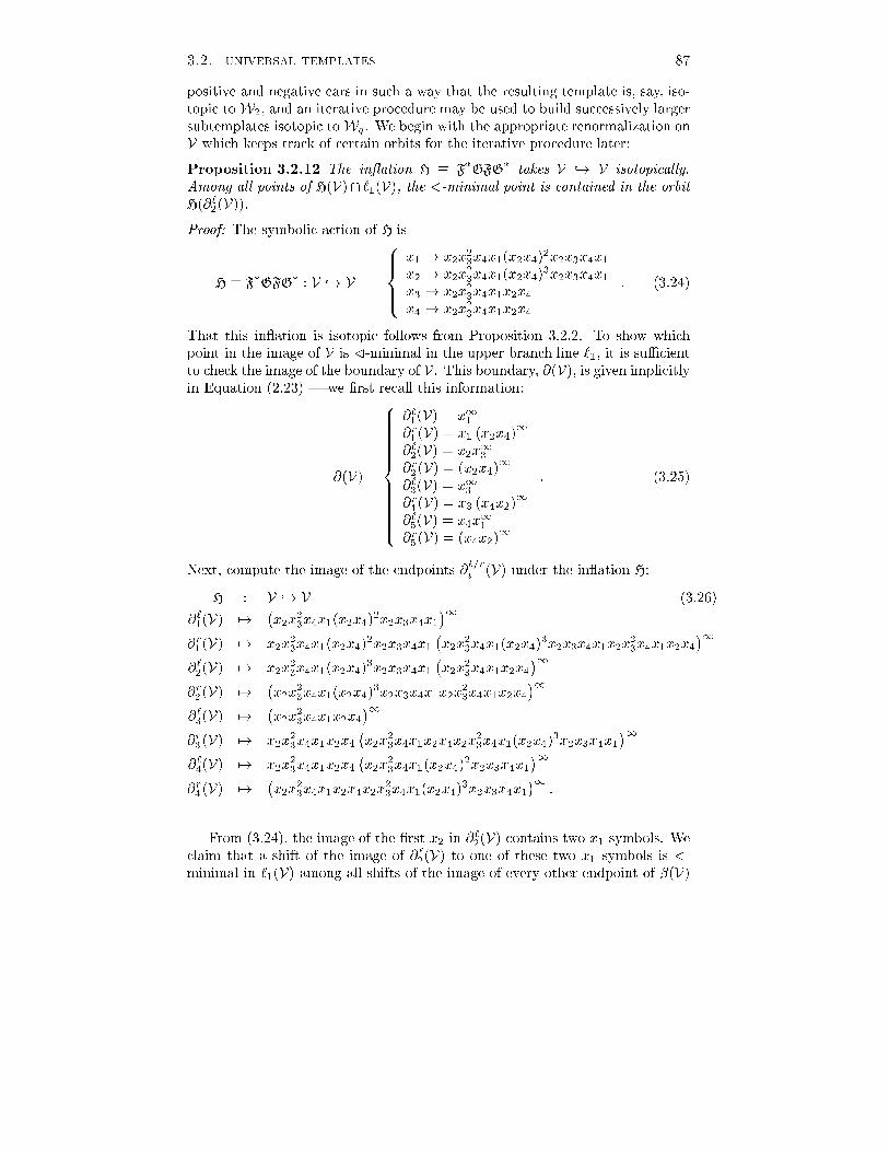
3.2. universal templates 87positive and negative ears in such a way that the resulting template is, say, iso-topic toW2, and an iterative procedure may be used to build successively largersubtemplates isotopic toWq. We begin with the appropriate renormalization onV which keeps track of certain orbits for the iterative procedure later:Proposition 3.2.12 The in ation H � F�GFG� takes V ,! V isotopically.Among all points of H(V)\ `1(V), the �-minimal point is contained in the orbitH(@2(V)).Proof: The symbolic action of H isH � F�GFG� : V ,! V 8>><>>: x1 7! x2x23x4x1(x2x4)2x2x3x4x1x2 7! x2x23x4x1(x2x4)3x2x3x4x1x3 7! x2x23x4x1x2x4x4 7! x2x23x4x1x2x4 : (3.24)That this in ation is isotopic follows from Proposition 3.2.2. To show whichpoint in the image of V is �-minimal in the upper branch line `1, it is suÆcientto check the image of the boundary of V . This boundary, @(V), is given implicitlyin Equation (2.23) | we �rst recall this information:@(V) = 8>>>>>>>>>><>>>>>>>>>>:

@1(V) = x11@r1(V) = x1 (x2x4)1@2(V) = x2x13@r2(V) = (x2x4)1@3(V) = x13@r4(V) = x3 (x4x2)1@5(V) = x4x11@r5(V) = (x4x2)1 : (3.25)Next, compute the image of the endpoints @`=ri (V) under the in ation H:H : V ,! V (3.26)@1(V) 7! �x2x23x4x1(x2x4)2x2x3x4x1�1@r1(V) 7! x2x23x4x1(x2x4)2x2x3x4x1 �x2x23x4x1(x2x4)3x2x3x4x1x2x23x4x1x2x4�1@2(V) 7! x2x23x4x1(x2x4)3x2x3x4x1 �x2x23x4x1x2x4�1@r2(V) 7! �x2x23x4x1(x2x4)3x2x3x4x1x2x23x4x1x2x4�1@3(V) 7! �x2x23x4x1x2x4�1@r3(V) 7! x2x23x4x1x2x4 �x2x23x4x1x2x4x2x23x4x1(x2x4)3x2x3x4x1�1@4(V) 7! x2x23x4x1x2x4 �x2x23x4x1(x2x4)2x2x3x4x1�1@r4(V) 7! �x2x23x4x1x2x4x2x23x4x1(x2x4)3x2x3x4x1�1 :From (3.24), the image of the �rst x2 in @2(V) contains two x1 symbols. Weclaim that a shift of the image of @2(V) to one of these two x1 symbols is �-minimal in `1(V) among all shifts of the image of every other endpoint of �(V)

88 chapter 3. template theorywhich begin with x1. That this is so is a simple matter of choosing the shift ofthe image of @2(V) which is �-minimal in �1(V) and then comparing this to allsuch shifts of the other endpoints H(@`=ri (V)). Using the �-ordering, this can bedone by hand or (more conveniently) by computer. In this manner, we calculatethat �14H(@2(V)) = x1 �x2x23x4x1x2x4�1 (3.27)is �-minimal among all other orbits in the image of H in `1(V), where � denotesthe shift operator. 2Note that the �-minimal point in H(V) on `1 is not x11 | thus, we mayuse this renormalization to append positive ears. The conjugate in ation will beused to append negative ears:Proposition 3.2.13 The in ation H� � FG�F�G takes V ,! V isotopically.Among all points of H�(V)\`2(V), the �-minimal point is contained in the orbitH�(@4(V)).Proof: Since H is isotopic, so is the conjugate H� via Lemma 3.2.4. Apply � toEquation (3.27) to show that��14H(@2(V)) = �nx1 �x2x23x4x1x2x4�1o (3.28)is �(�)-minimal in �(`1(V)); after an application of Lemma 3.2.3 and the factthat � commutes with the shift operator �,�14�H(@2(V)) = x3 �x4x21x2x3x4x2�1 (3.29)is �-minimal in `2(V). Now insert �2 in the domain. Since � is involutive, wehave shown that�14�H�(�@2(V)) = �14H�(@4(V)) = x3 �x4x21x2x3x4x2�1 ; (3.30)is �-minimal in `2(V). 2We may now complete the major step in the proof of Theorem 3.2.8.Theorem 3.2.14 The template Wq appears as a subtemplate of V for all q > 0.Proof: As we will be working with a series of distinct copies of the template V ,we introduce some notation. Let fV ig denote a sequence of distinct copies of theembedded template V | each is embedded in a di�erent copy of S3. Constructan alternating sequence of templates and isotopic in ations:V1 H�! V2 H��! V3 H�! V4 H��! V5 H�! V6 H��! � � � (3.31)By Proposition 3.2.12, we may append a positive ear to H(V1) in V2 along theimage of @2(V1), creating the template denoted W+1 � V2. This subtemplate

3.2. universal templates 89contains the orbit @4(V2). By mapping V2 into V3 via H�, we push W+1 toa deeper isotopic copy within V3. A negative ear may then be appended toH�(W+1 ) � V3 along H�(@4(V2)) according to Proposition 3.2.13. Since thenegative ear is appended along an interval having endpoint on H�(@4(V2)), theappended negative ear \precedes" the formerly appended positive ear (in thesense of the ow-direction), yielding a subtemplate of V3 isotopic to W2: seeFigure 3.13. H H�(+) ear (�) ear@2(V1) @4(V2)H �@2(V1)� @2(V3)H �@4(V2)�H�H �@2(V1)�(a) W1 (b) W+1 (c) W2Figure 3.13: The steps in building Wq.We now have the template V3 containing a subtemplate isotopic toW2 whichcontains the orbit @2(V3). Since V3 is again an isotopic copy of V1 with @2(V3)corresponding to @2(V1), we may now iterate the procedure. Map V3 into V4via H, append a positive ear to the image of W2 to obtain W+2 , then apply H�and append a negative ear to the image of W+2 to produce W3. Since all thein ations involved are isotopic, we continue to carry the completed Wi alongisotopically as we append additional ears. Thus, we can embed Wq in V forarbitrary q. 2Proof of Theorem 3.2.8: According to Theorem 1.1.13, any link may be repre-sented as some closed braid. By Proposition 3.2.9, this closed braid must appearon Wq for q suÆciently large; hence, by Theorem 3.2.14, this link lives on V . 23.2.3 Universal templatesDe�nition 3.2.15 A universal template is a template T � S3 among whoseperiodic orbits are representatives of every link type.

90 chapter 3. template theoryFrom Theorem 3.2.8, we may show the abundance of universal templates.Proposition 3.2.16 The Lorenz-like templates L(0; n) are universal for n < 0Proof: In Figure 3.14, we show the image of the in ationL : U ,! L(0;�2) 8>><>>: x1 7! x1x2 7! x31x2x3 7! x2x1x4 7! x2x1x2 : (3.32)It is a (challenging!) exercise for the reader to show that this image is isotopicto U . By Propositions 3.2.2 and 3.2.1, there is a subtemplate chainV � U � L(0;�2) � L(0;�4) � L(0;�6) � � � �� L(0;�1) � L(0;�3) � � � � : (3.33)The result now follows from Theorem 3.2.8. 2

Figure 3.14: The template U is a subtemplate of L(0;�2).Given some embedded template, it is often relatively easy to recognize aLorenz-like subtemplate; hence, we have a useful test for identifying universaltemplates.Corollary 3.2.17 SuÆcient conditions for a template T � S3 to be universalare

3.2. universal templates 911. There is a two-component unlink on T ; that is, there exist two separableunknots.2. One component of the unlink is untwisted; the other is twisted with � 6= 0twists.3. The two unknots intersect some branch line of T in two adjacent points(recall De�nition 3.1.5) The sign of the branch line crossing between thesetwo points must be opposite that of the twist � .Proof: Let a1 and b1 denote the adjacent points in �`j , with b1 denoting theorbit with twist � . For � < 0, the template in ationL(0; �) ,! T � x1 7! ax2 7! b (3.34)is isotopic, since a1 and b1 are an unlink and there is agreement betweentwisting and branch line orientation. For � > 0, the same symbolic map sendsthe mirror image of L(0;��) into T isotopically. However, the mirror image ofa universal template is also universal. 2We may use Corollary 3.2.17 to show that certain hyperbolic ows on S3contain all links as periodic orbits: e.g.,Proposition 3.2.18 The suspension of the Plykin map, given in Example 2.1.6,when embedded in S3 in the \standard" way, yields a ow having all link-typesas periodic orbits.Proof: Recall the Plykin attractor �P described in Example 2.1.6. The inverselimit construction of Williams implies that we can collapse the attractor for themap to a branched one-manifold which suspends to a semi ow on a branchedtwo-manifold3. In Figure 3.15, we show two periodic orbits in the suspension ofthe Plykin graph. The �rst orbit, a, has period one, is untwisted, and is clearlyseparable from all other orbits. The second orbit, b, is an unknot.It is not hard to see that b must be a twisted orbit; however, even if it werenot, we could use Proposition 3.1.19 and Corollary 3.1.10 to show the existenceof another orbit which is a twisted unknot separable from a. Finally, we donot need to know the sign of the twist, since on the \branch line" (the graph�P ), the orbit a is adjacent to a point of b on either side, so it has branch linecrossings of both types; hence, by Corollary 3.2.17, the periodic orbits of this ow contain all link types. 2Corollary 3.2.17 is genuinely useful in this instance, since it is very diÆcultto draw an accurate picture of the entire template for the suspended Plykinattractor. The Plykin attractor is the simplest hyperbolic planar attractor. Wehave examined a few other examples and have managed to show that these alsogive rise to universal templates: we do not know of an example which does not.3Though the suspension of the Plykin graph does not satisfy the de�nition of a template,it may be thought of as a template with the boundaries sewn together.

92 chapter 3. template theory a b

�P

Figure 3.15: The suspension of the Plykin attractor | top are bottom areidenti�ed. Two orbits, a and b, form a \spine" for a universal subtemplate.Corollary 3.2.19 There exists a structurally stable vector �eld on S3 such thatthe induced ow on S3 contains closed orbit representatives of all knot and linktypes.Proof: The Plykin map suspends to a ow on D2 � S1 which is inwardly trans-verse on the boundary and has chain recurrent set consisting of three attractingperiodic orbits and the suspended Plykin attractor. Complete the ow on S3 bytaking another D2 �S1 having a single repelling periodic orbit as f0g� S1 andoutwardly transverse at the boundary and gluing these two solid tori togetherto get S3 (a more detailed treatment of this construction appears in xA.1). Theresulting ow has a hyperbolic chain recurrent set and hence, by Theorem 1.2.14,is structurally stable to C1 perturbations. 2Remark 3.2.20 There are numerous examples of ows on S3 having all linktypes as periodic orbits. In x4.4, we will show that ows arising from certain\simple" ordinary di�erential equations can be modeled with a universal tem-plate. In [69], it was shown that certain �bred knots, namely the �gure-eightknot and the Borromean rings, have complement �bred by a �bration whose in-duced ow contains all links as orbits (recall x2.3.4). As an exercise, the readermay wish to �nd two orbits on the template for the Whitehead link complement,Figure 2.17, which satisfy the conditions of Corollary 3.2.17, showing that thisalso is a universal template.The Lorenz-like templates are the simplest class of templates: they have twounknotted unlinked strips with one branch line. A complete classi�cation of

3.2. universal templates 93these templates into universal and non-universal would be useful, cf. Corollary3.2.17. At this time, we can o�er only the following:Proposition 3.2.21 For mn � 0, the Lorenz-like template L(m;n) is universalif and only if m or n is 0 and the other index is negative.Proof: Proposition 3.2.16 covers the case where one number is zero and the otheris negative: we will show that all other cases with mn � 0 are not universal. Inthe case where m and n are both nonnegative, the template L(m;n) containsonly positive crossings and therefore carries no knots with mixed crossings (suchas the �gure-eight knot). Next, consider the case where m and n are bothnegative. Let Ka and Kb be two distinct knots on L(m;n) which form a link.If L(m;n) were universal, there would be an in�nite number of distinct choicesfor Ka and Kb which would span all possible linking numbers. We compute thelinking number as one half the algebraic sum of the total number of crossings,C, as per Equation (1.2). The crossing number, C, can be decomposed into thesum C = Cm + Cn + Co; (3.35)where Cm equals the contribution due to the m half-twists along the x1 strip,Cn equals the contribution due to the n half-twists along the x2 strip, and Coequals the number of crossings due to the overlap of the x1 strip over the x2strip at the branch line. Denote by aij (resp. bij) the number of xixj blocks inthe periodic itinerary of Ka (resp. Kb). Example: if Ka = �x1x22x1x2�1, thena11 = 0; a12 = a21 = 2, and a22 = 1. We note that in all cases,a12 = a21; b12 = b21: (3.36)We can calculate the crossing numbers Cm and Cn:Cm = m(a11+a12)(b11+ b12) � 0; Cn = n(a21+a22)(b21+ b22) � 0: (3.37)We will maximize the crossing numbers in order to obtain upper bounds;hence, we assume that there is a minimal amount of negative twisting in thestrips, thereby setting m = n = �1 in Equation (3.37). To maximize theovercrossing number Co, we again assume that all potential crossings can infact occur. This situation is displayed schematically in Figure 3.16, where thedi�erent strands do not represent the knots themselves, rather those portionsof the knots which correspond to the numbers a11, etc. From Figure 3.16, thecrossing number is bounded above byCo � a12b21 + a21b12 + a11b21 + a21b11 + a22b12 + a12b22: (3.38)Combining this with Equations (3.35) and (3.36) yieldsC � 2a12b12 + a11b12 + a12b11 + a22b12 + a12b22 � a11b11 � a11b12�a12b11 � a12b12 � a12b12 � a12b22 � a22b12 � a22b22� �(a11b11 + a22b22)� 0 :(3.39)

94 chapter 3. template theorya11 b11 a12 b12 b21 a21 b22 a22

Figure 3.16: A schematic diagram of crossings on the template L(�1;�1): eachstrand labeled aij (resp. bij) represents a collection of aij (resp. bij) strands ofthe knot Ka (Kb) which begin on the strip xi and end on the strip xj .Hence, the linking number `k(Ka;Kb) is at most zero and L(m;n) cannot sup-port all links. 2We have classi�ed the universal Lorenz-like templates in every case exceptm < 0; n > 0 (and vice versa). The linking number estimates in the proof donot yield the necessary results in the case when m and n are of mixed sign. Wesettle for the following:Conjecture 3.2.22 A Lorenz-like template L(m;n) supports all links if andonly if either m or n is zero and the other index is negative.The most pressing problem concerning universal templates is to determine asimple set of necessary and suÆcient conditions for universality. We concludewith two related conjectures.Conjecture 3.2.23 An embedded template T � S3 is universal if and only ifit contains V as a subtemplate.

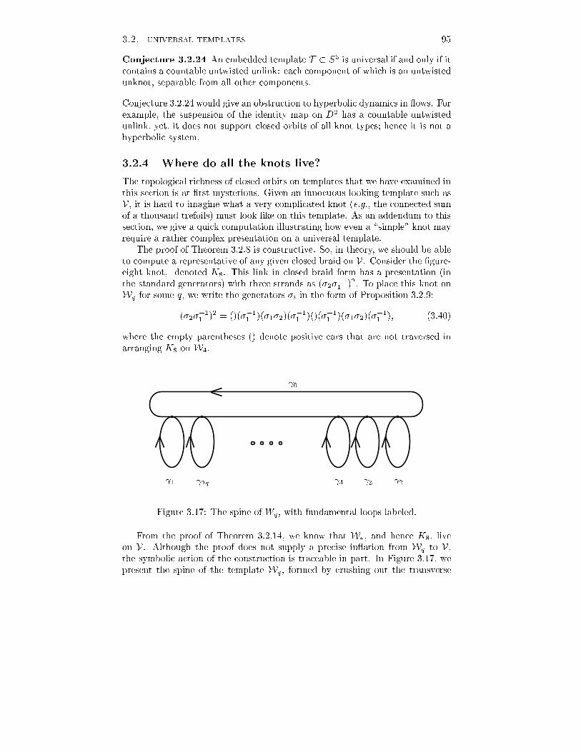
3.2. universal templates 95Conjecture 3.2.24 An embedded template T � S3 is universal if and only if itcontains a countable untwisted unlink: each component of which is an untwistedunknot, separable from all other components.Conjecture 3.2.24 would give an obstruction to hyperbolic dynamics in ows. Forexample, the suspension of the identity map on D2 has a countable untwistedunlink, yet, it does not support closed orbits of all knot types; hence it is not ahyperbolic system.3.2.4 Where do all the knots live?The topological richness of closed orbits on templates that we have examined inthis section is at �rst mysterious. Given an innocuous looking template such asV , it is hard to imagine what a very complicated knot (e.g., the connected sumof a thousand trefoils) must look like on this template. As an addendum to thissection, we give a quick computation illustrating how even a \simple" knot mayrequire a rather complex presentation on a universal template.The proof of Theorem 3.2.8 is constructive. So, in theory, we should be ableto compute a representative of any given closed braid on V . Consider the �gure-eight knot, denoted K8. This link in closed braid form has a presentation (inthe standard generators) with three strands as (�2��11 )2. To place this knot onWq for some q, we write the generators �i in the form of Proposition 3.2.9:(�2��11 )2 = ()(��11 )(�1�2)(��11 )()(��11 )(�1�2)(��11 ); (3.40)where the empty parentheses () denote positive ears that are not traversed inarranging K8 on W4. 0 1 2 3 4 2qFigure 3.17: The spine of Wq , with fundamental loops labeled.From the proof of Theorem 3.2.14, we know that W4, and hence K8, liveon V . Although the proof does not supply a precise in ation from Wq to V ,the symbolic action of the construction is traceable in part. In Figure 3.17, wepresent the spine of the template Wq, formed by crushing out the transverse

96 chapter 3. template theorydirection to the semi ow. The generators of the fundamental group of Wq arelabeled 0; 1; : : : ; 2q in the order in which they are constructed within V . Bycarefully following the proof of Theorem 3.2.14, one can track the images of theseloops i in V for the \simplest" copy of Wq in V :i i 2 �1(Wq)0 (H�H)q�1(x2x4) = �FG�(F�G)2FG��q�1 (x2x4)1 (H�H)q�1(x1) = �FG�(F�G)2FG��q�1 (x1)i = 2k > 0 (H�H)q�k(x3) = �FG�(F�G)2FG��q�k (x3)i = 2k + 1 > 1 (H�H)q�k�1H�(x1) = �FG�(F�G)2FG��q�k�1 FG�F�G(x1)(3.41)From this table, we could compute the symbol sequence of this representativeof K8 in V ; however, printing it out might take more room than our publisherwishes to spare. We merely compute the symbolic period, i.e., the length of therepeating block of the periodic word.The knot K8 on W4 determines a word in �1(W4) in the i generators | letni, i = 0 : : : 8 denote the number of i terms in this word. In other words, thelink K8 goes around the loop i exactly ni times. To compute j ij, the symboliclength of the image of the loop i in V , we de�ne a symbolic growth matrix fora template renormalization.De�nition 3.2.25 Given a renormalization R : T ,! T , where T has Markovpartition fx1; x2; : : : ; xNg, de�ne the growth matrix of R, GR 2 MN(Z+), asfollows: GR(xi; xj) = f# of xi symbols in R(xj)gg (3.42)Lemma 3.2.26 For any R and ~R : T ! T ,GR ~R = GRG ~R: (3.43)Proof: This follows from De�nition 3.2.25 and the fact that the number of xisymbols in R ~R(xj) equalsGR ~R(xi; xj) =Xk GR(xi; xk)G ~R(xk ; xj) = hGRG ~Ri (xi; xj): (3.44)2We compute the growth matrices for the renormalizations H and H� fromEquations (3.24) and (3.20) to beGH = 2664 2 2 1 14 5 2 23 3 2 24 5 2 2 3775 GH� = 2664 2 2 3 32 2 4 51 1 2 22 2 4 5 3775 : (3.45)Hence, by using Lemma 3.2.26 and the information from (3.41), we can computethe growth matrix for the renormalization which takes each i into V . Thisinformation yields the length of the orbit i in V :

3.3. subtemplate structures 97Example 3.2.27 To �nd j 0j for W4 � V , we look up 0 from (3.41) and notethat it is the image of (x2x4)1 under (HH�)3. To count j 0j, the length, set~v = [0; 1; 0; 1]t and take the product �GHGH��3 ~v. Then sum all the entries ofthis column matrix | from De�nition 3.2.25, this counts the number of x2 andx4 elements, giving the length j 0j.i ni j ij i ni j ij0 3 3387648 5 0 8391 0 1990365 6 1 772 1 1086485 7 1 73 1 99679 8 1 14 1 9145 (3.46)Finally, to obtain the length of the representative of the �gure-eight knot K8in V , a simple computation from (3.46) gives:jK8j = 8Xi=0 nij ij = 11; 358; 338; (3.47)or, over eleven million. There are surely simpler representatives of K8 on V ;however, the simplest may still be outside of the range in which one can drawit.4This example illustrates that methods used in the proof of Theorem 3.2.8extract relatively \deep" information from templates.Remark 3.2.28 To compute upper bounds for the minimal length of a givenknot type represented on V , one need merely compute the Perron-Frobenius(i.e., maximal) eigenvalue of the growth matrix GH | it is about 10.332. Then,given any knotK, write it in braid format which is compatible with the templateWq , as done in Equation (3.40). Note that the length jKj of the resulting braidword may be quickly estimated from any braid version of L via the procedure ofProposition 3.2.9. A (poor) lower bound for the length of an orbit representingK is then given by (10:332)jKj�1, since then in ation H (or H�) must be appliedjKj � 1 times to �t Wq with the braid form of K on it within V . Applied tothe �gure eight example with braid length 8 (from Equation (3.40)), one getsan upper bound for the minimal length as 12; 567; 447 | o� from our computedexample by about ten percent.3.3 Subtemplate structuresAlthough the results of Theorem 3.2.8 are exciting, we have, to some degree,drawn our conclusions too soon. The proof succeeds because it examines sub-template structures, which carry the desired links, rather than examining the4Two of us (MS, RG) tried very hard to �nd a copy of K8 on V or U before Theorem 3.2.8was discovered.

98 chapter 3. template theoryindividual knots and links per se: the crucial step lies in showing Wq � V . Webegin this section by resuming our study of the subtemplates of V . The results ofthis line of inquiry will lead to generalizations of Theorem 3.2.8 and will suggestdirections for further investigation along the lines of subtemplate structures. Wedo not present all the results in full detail: the interested reader should be ableto �ll in such as necessary.We must distinguish between orientable and nonorientable cases, since anorientable template cannot contain any nonorientable subtemplates. In x3.3.1and x3.3.2, we prove the existence of templates which are \universal" in theclasses of orientable and nonorientable templates in that they contain isotopiccopies of all [orientable] templates as subtemplates.3.3.1 Orientable subtemplatesWe begin with a generalization of the braid group structure of De�nition 1.1.11to a semigroup structure on braided templates. The generators of the semigroupare of three types:1. ��i , is a \ at ribbon" version of the generators for the braid group: theith strip crosses over the (i + 1)st in the positive sense. These elementsare invertible;2. ��i , is the trivial element (a collection of straight at strips) with the ithstrip given a half twist, either in the positive (�i) or negative (��1i ) sense.These elements are invertible.3. ��i , is a branch line chart with the ith and (i + 1)st strips incoming, koutgoing strips5, and either a positive (�i) or a negative (��1i ) crossing atthe branch line. These generators are not inverses, as branch lines cannotbe cancelled under composition.Figure 3.18 illustrates the generators.The following result is obvious, and implicit in the proof of Theorem 3.1.2[58]:Lemma 3.3.1 The set f��i ; ��i ; ��i g generates the class of braided templates.With the braided template semigroup playing the role of BN in Theorem3.2.8, we may generalize this result to:Theorem 3.3.2 The template V contains every embedded orientable templateS as a subtemplate. Furthermore, these may be chosen so as to be disjoint andseparable.Proof: Recall Theorem 3.2.14 | V contains Wq for all q. The strategy of theproof of Theorem 3.2.8 was to show that any given closed braid can be �tted5For simplicity, we suppress reference to the number of strips involved, which varies through-out the braid presentation, in our notation.

3.3. subtemplate structures 99

(a) (b) (c)Figure 3.18: The generators for the braided template semigroup: (a) �i; (b) �i;(c) �i.onto someWq. We use the semigroup for braided templates in analogous fashionto show that all orientable templates also live on Wq , and hence on V .Consider S a template in S3, presented as a at braided template as perTheorem 3.1.2. To show that such a given template lives as a subtemplate ofWq for some q, we will express each generator as a subtemplate of a portion ofWq ; that is, on a �nite sequence of alternating ears.In Figure 3.19, we exhibit a portion of a subtemplate on a pair of positive andnegative ears which corresponds to the generator �1�2 : : : �k for any desired k.Note that the belt trick is used in concert with two ears of opposite sign to cancelthe full twist induced by going around an ear. One constructs the generator��11 ��12 : : : ��1k in analogous fashion. To show that some �nite product of theseyields �j and ��1j for any j, we follow the same argument as in Proposition 3.2.9.To show that �i and ��1i appear likewise, we turn to Figure 3.20, whichcontains a local picture of the generator �i. The �rst i strips travel around anegative ear and then a positive ear (or vice versa for ��1i ) in order to cancelthe twisting and allow for a positive (negative resp.) crossing at the branch line.Since an orientable braided template may always be made at, we do notneed to �t powers of �i on Wq; hence, the entire generating set for braidedorientable templates appears locally on a �nite set of alternating positive andnegative ears. Pieceing together local submanifolds on Wq is always possible aslong as the number of strips matches | after including all the crossings, branchlines, etc., one simply connects the top to the bottom strips in the standardway. Hence, given any template presented in these standard generators, onemay construct for some q (perhaps very large) a subtemplate of Wq which isisotopic to the intended template.The result then follows from Theorem 3.2.14. 2

100 chapter 3. template theory

Figure 3.19: The braided-template word �1�2 : : : �k lives on a pair of alternatingears.Remark 3.3.3 Theorem 3.3.2 indicates that, among the class of orientable tem-plates, V is not merely an example of an exceptional template: it (and all othersuch templates) truly deserves the title of universal template, since a templatecontains all orientable templates if and only if it contains V .Corollary 3.3.4 The template V contains all evenly twisted links: that is, itcontains all links indexed by the (even) twist of the local stable manifolds (seeDe�nition 3.1.9).Proof: Given an indexed link L, where the components of L are indexed by thetwist, build an orientable template TL which contains the link L as its \spine."More speci�cally, form a connected graph from L by (arbitrarily) identifyingpoints on components pairwise. Then, thicken the graph up to a template,adding branch lines at vertices and twisted strips along the edges as appropri-ate: cf. Figure 3.9(b). This template, which contains L as a set of periodicorbits, lives on V by Theorem 3.3.2. 2Our next result shows that any orientable template may be embedded in S3as a universal template (and then some):Theorem 3.3.5 Any orientable template T may be embedded in S3 so as to

3.3. subtemplate structures 101

Figure 3.20: The generator �i lives on a pair of alternating ears.contain an isotopic copy of all orientable templates as disjoint separable subtem-plates.Proof: Assume for the moment that, for some branch line `j , there exist twoperiodic points of �`j , a1 and b1, such that each symbol xi in the Markovpartition of T appears at most once in the word ab; thus, each strip of Tcontains at most one strand of the link fa1;b1g.Re-embed T by changing the overcrossings of strips in the given planar pre-sentation in the manner to be described: by the above condition, whenever theknots corresponding to a1 and b1 cross one another, they must do so on sep-arate strips. Re-embed T so as to force the strip containing the orbit a1 toalways be on top. In this embedding, then, the two knots are clearly separable.Now restrict attention to those instances where the knot corresponding toa1 crosses itself: if a and b are chosen as above, this crossing must be due to astrip crossing over itself or another strip. Beginning at an arbitrary point on thisorbit, follow along the direction of the ow | whenever there is a self-crossing,re-embed the strips so that the desigated point is on top. When �nished, onehas a knot which can be perturbed so as to have a unique local maximum: anunknot. Repeat this procedure for the knot b1, noting that one is not tamperingwith any previously re-embedded strips.Finally, build a Lorenz-like subtemplate of T given by the image of the in a-tion x1 7! a; x2 7! b, as in Equation (3.13) in Corollary 3.1.17. Since the orbits

102 chapter 3. template theorycorresponding to a1 and b1 are unknotted and separable, the subtemplate inthe particular embedding of T we have chosen is isotopic (up to taking the mir-ror image) to the Lorenz-like template L(�a; �b) for some even numbers �a; �b,depending on twist. Change the embedding of T by adding full twists to selectedstrips so that the subtemplate is isotopic to L(0;�n) (or its mirror image), forpositive n, which contains all orientable templates as separable subtemplates.To conclude, we must verify our assumption that a1 and b1 exist. First,we eliminate certain troublesome strips. If a particular branch line `j has onlyone outgoing strip, we may have to choose a and b to both travel down thisstrip. To avoid any problems associated with this, we perform an isotopy onT within a tubular neighborhood of T in S3. This isotopy has the e�ect ofpushing the branch line `j forwards (in the sense of the semi ow) along theone outgoing strip until it is almost identi�ed with the next branch line: seeFigure 3.21. Under such an isotopy, any crossings that this unique outgoingstrip was formerly involved with are now subsumed by crossing of other strips(including twisting in the original strip). Thus, we can ignore orbits which traveldown this strip in the above arguments, and, in identifying the shrunken stripto the next branch line, we assume that every branch line chart contains at leasttwo outgoing strips.

Figure 3.21: One can \eliminate" a single-outgoing strip by propagating thebranch line forwards.Next, choose a �nite admissible orbit a1. We claim that a may be chosensuch that the knot passes through each branch line at most once. Assume thata = a1a2a3, where a2 and a3 are words whose orbits begin from the same branchline. Then, replace a with a1a3: this is an admissible word since incoming stripsstretch over branch lines completely. Iterating this reduction on a word of �nitelength is a terminal process.Finally, we claim that b may be chosen similarly to have no symbols in com-mon with a. Recall, we have modi�ed T to have [in e�ect] at least two outgoing

3.3. subtemplate structures 103strips per branch line chart, and a intersects each branch line at most once.Beginning at some branch line of T , choose an outgoing strip whose symbol isnot part of a | this is always possible since there are more than two outgoingstrips. This outgoing strip leads to another branch line. Repeat the processof choosing outgoing strips avoiding a until the branch line is repeated: thisde�nes a periodic orbit a0. If a0 and a have a branch line in common, this isthe desired b. If not, repeat the process of choosing another periodic orbit a00| this algorithm may be repeated since there are again at least one incomingand outgoing strips per branch line on T minus the strips of a and a0. Since theMarkov partition is �nite, this is a �nite process; hence, a and b may be chosenas above. 2Corollary 3.3.6 Any embedded orientable template T contains a (nonisotopi-cally) embedded copy of every orientable template.3.3.2 Nonorientable subtemplatesThe nonorientable case is quite a bit more subtle, but is solved in similar fashion.We leave the [numerous] details of the following theorem to the reader.Theorem 3.3.7 There exists a template which contains every embedded tem-plate S as a subtemplate.Idea of Proof: We begin with the template L(0;�2), which contains V via thein ation LG, where L : U ,! L(0;�2) is the in ation of Equation (3.32). Then,we append an extra ear to this template which is twisted and separable from theremainder of the template: see the template Y in Figure 3.22. Given any tem-plate, we then show that it may be obtained by �rst placing a similar orientabletemplate on L(0;�2), then diverting some of the strips around the twisted ap-pended ear of Y to produce the requisite nonorientable subtemplate.Let S be an arbitrary embedded template in S3. We brie y indicate how toplace S in the appropriate form for being a subtemplate of Y .Step 1: Place S in braided form as per Theorem 3.1.2, and represent thistemplate in the braid semigroup of Lemma 3.3.1.Step 2: Factor this braid word so that there is a positive half-twist � onthe �rst k strips, where � is the word� = �1�2 � � � �k k�1Yi=1 �1�2 � � ��i! ; (3.48)followed by a braid word having no ��i terms.Step 3: For S braided into the word above, let ~S denote the at orientabletemplate given by removing the initial word � from the braid word. Map ~Sinto L(0;�2) � Y isotopically via the in ation LGI, where I : ~S ,! V is thein ation from the proof of Theorem 3.2.8 and L : U ,! L(0;�2) is the in ationfrom Equation (3.34).

104 chapter 3. template theoryx2 x3x4x1

Figure 3.22: The template Y contains all templates as subtemplates.Step 4: Now, by carefully tracking the placement of the �rst k strips inS � Y , modify the in ation in the appropriate manner to \divert" the leftmostk strips of S on Y to instead make a loop around the appended twisted x1-ear.This has the e�ect of inserting � into the braid word for ~S at the beginning.This new template is the original S by Step 3. 2Corollary 3.3.8 The template Y contains isotopic copies of links with arbitrarytwist type.Proof: See the proof of Corollary 3.3.4. 2Remark 3.3.9 Note that although Y contains all embedded templates as dis-joint subtemplates, these may not be chosen so as to be mutually unlinked inthe present construction, since there is a linking induced by the trip about thetwisted ear. We believe that this is unavoidable: i.e., no embedded templatecontains disjoint unlinked copies of all embedded templates as subtemplates.We do not believe that the results of Theorem 3.3.5 hold for nonorientabletemplates: that is, we do not believe it is possible to re-embed, say, the horse-shoe template L(0; 1) in such a way that it contains copies of every embeddedtemplate, or even the orientable ones. A related, though weaker statement ishowever true:Proposition 3.3.10 Any embedded non-orientable template T contains a (non-isotopically) embedded copy of all templates.Proof: If T is nonorientable, we must construct an in ation from the templateY of Figure 3.22 into T . Take a1 twisted and b1 untwisted with the pair

3.3. subtemplate structures 105adjacent. Then consider c = a2b: c1 is an untwisted orbit with a1 and c1adjacent and �ba2�1 and b adjacent. Hence, there is a well-de�ned templatein ation, R : Y ,! T 8>><>>: x1 7! ax2 7! a2x3 7! bx4 7! b : (3.49)As this in ation is nonisotopic, we have a di�erent embedding of all the subtem-plates of Y into T . 2Ostensibly, it seems surprising that the template for the Whitehead linkcomplement (Figure 2.17) embeds in the horseshoe template L(0; 1).Remark 3.3.11 Although the results of this section are exciting, they may alsobe cause for concern in certain applications: recall from x2.3.5 the constructionof induced templates from time series data. Ko�carev et al. derive an inducedtemplate in [106] which, by appealing to Theorem 3.3.7, we can show containsall embedded templates as subtemplates. In the literature on induced templates,it is implicit that the \physical" system may be expected to contain merely asubset of the knots and links on the induced template. Hence, the use of thisinduced template would appear to be of limited applicability | it contains fartoo much.Remark 3.3.12 The theorems of this section can be applied to the problem ofaccumulations of knots on a template from x3.1. In contrast to Theorem 3.1.20,universal templates have no restrictions on the types of accumulations of knots.Theorem 3.3.13 (Ghrist [68]) Let fKig be an arbitrary sequence of knot types,and let K be any chosen knot type. Then, on the universal template V, thereexists a sequence of distinct closed orbits f ig of knot type Ki, which accumulatesonto a closed orbit of knot type K.This theorem sheds light on the class of in�nite links contained in universaltemplates: of course, not every in�nite link may live on a template, but there isno obstruction as far as accumulations of knot types goes.Remark 3.3.14 A template contains both topological and dynamical informa-tion. By \forgetting" the topology, one reduces a template to a purely dynamicalobject. For example, if one takes the set of branch lines as a cross-section to thesemi ow, on obtains a set of coupled, expanding, one-dimensional maps. Or,if one collapses a template along the direction transverse to the semi ow, oneobtains a directed graph, which de�nes a subshift of �nite type (cf. Remark1.2.22). Theorems 3.3.2 and 3.3.7 then yield as a scholium a dynamical result:Corollary 3.3.15 Let (�A; �) be an irreducible subshift of �nite type. Givenany N�N matrix of zeros and ones, B, there exists a local cross section �0 � �Asuch that the return map r acting on this cross section is conjugate to the subshiftde�ned by �B.

106 chapter 3. template theoryA similar result holds with renormalizations of coupled, expanding one-dimensional maps. These dynamical results are, if not well-known, then at leastprovable through much simpler methods than those of this chapter. Yet, we notethat the methods used in this chapter are by-and-large topological: Alexander'sTheorem, braid groups, etc., are key tools. Thus, we are pleased that knot-theoretic tools can be brought to bear on a dynamical problem. In the nextchapter, too, such tools will be shown to be useful in studying bifurcations ofparametrized families of ows.

Chapter 4: BifurcationsIn Chapter 3 we derived general results on template knots and links. The themewas one of richness and inclusion: every template contains in�nitely many dis-tinct knot types; templates carrying unlinked, unknotted, untwisted orbits sup-port in�nite sequences of isotopic knots, and, most strikingly, \many" templateswith mixed crossings carry all knots and links (and even all templates).We now turn to issues of uniqueness and exclusion, asking how knowledge ofknotting and linking data implies restrictions on families of periodic orbits andthe bifurcations in which they are created. More speci�cally, in a parametisedfamily of ows, periodic orbits appear and disappear in [often complicated] se-quences of bifurcations. But for three-dimensional ows, it is the link of periodicorbits which undergoes bifurcations. Thus, if (1) we \dress" the periodic orbitset with knotting and linking information; and (2) we compute the topologicalaction of bifurcations on orbits, we produce a set of bifurcation invariants derivedfrom knot theory. This chapter will be a brief tour through several applicationsof this principle.We begin with introductory remarks on local bifurcation and continuation oforbit branches and some elementary observations regarding the link structuresarising in saddle node and period-multiplying (doubling and Hopf) bifurcationsfrom closed orbits. In x 4.2 we describe a number of results on the horseshoetemplate H of Figure 2.9, the major ones being existence, non-existence anduniqueness theorems for families of torus knots of speci�ed dynamical periods.These provide invariants which distinguish orbits, permitting us to follow themfrom a chaotic hyperbolic set, back to their birthplaces in parameter space,thereby determining genealogies and orders of precedence in a family of H�enonmaps. Section 4.3 contains knot theoretic analogues of the self-similarity resultson bifurcation sequences of the quadratic family (1.23) introduced in x1.2.3.We show how a factorisation of kneading sequences corresponds to subtemplateswhich are embedded copies ofH, and indicate how this may be used to determinethe orbits implicated in iterated torus knots and more general cabled structuresinvolving horseshoe knots and links. Perhaps the major interest in this workis the way in which knot invariants a�ord a link (pun intended) between localbifurcations and global questions.In the �nal section we address global bifurcations more explicitly, describingsome periodic orbit structures that appear near homoclinic orbits to saddle-typeequilibria. We call attention to two types of topologically signi�cant global bifur-cations | the gluing bifurcations, and the bifurcations surrounding a Shil'nikovconnection. In the case of gluing bifurcations, the issue at hand is not richnessof orbits (primarily only \simple" knots appear), but of countable bifurcationsequences. In stark contrast, in the Shil'nikov scenario, we �nd a general case107

108 chapter 4. bifurcationsin which the universal template V of x3.2 is contained within the ow, therebygiving a set of (primarily dynamical) suÆcient conditions under which a givenODE contains all knots and links among its periodic orbits. We close with anexample of a piecewise linear ODE which satis�es the necessary hypotheses: anexplicit seed from which all knots and links can be grown.This chapter provides merely a sample of numerous results which have beenobtained for speci�c systems. For further examples, see [87, 93, 88, 70, 118, 119,180]. It is our hope that knotting and linking data will become increasingly usefultools in the subtle business of tracking global phenomena in the bifurcations ofperiodic orbits.4.1 Local bifurcations and linksIn x1.2.3 we described the three codimension-one bifurcations of maps: thesaddle-node, period-doubling, and Hopf bifurcations (we also noted the symmet-ric pitchfork bifurcation). In the associated three-dimensional ows obtained bysuspending these families, there are natural and simple implications for knottingand linking of the periodic orbits involved. Speci�cally, we have:Proposition 4.1.1 The periodic orbits implicated in a saddle-node or pitchforkbifurcation of a three dimensional ow are isotopic knots and have the samelinking number with any other orbit which persists through the bifurcation point.Proof: We discuss the saddle-node case, as that of the pitchfork is analogous.Consider the parametrised Poincar�e map on a small cross section to the owtransverse to the orbit at the bifurcation. Upon passing the parameter throughthe bifurcation, the �xed point becomes a pair of �xed points, one of which (sayp1) is a saddle, the other of which (say p2) is either a source or sink.In the case of p2 a source and for parameter suÆciently close to the bi-furcation, one branch of W s(p1) is a small segment contained in W u(p2) withendpoints p1 and p2. Hence, in the suspension of the return map, the two pe-riodic orbits form the boundary components of an embedded annulus, and arethus isotopic. 2Proposition 4.1.2 The periodic orbits created in period-doubling and Hopf bi-furcations are cables of the original (bifurcating) orbit.Proof: Following the proof of Proposition 4.1.1, one notes that the orbit ofperiod 2T created in period-doubling bifurcation is the boundary of a M�obiusband formed of the two-dimensional stable (or unstable) manifold associatedwith the eigenvalue of the Poincar�e map passing through �1, whose core is theoriginal period T orbit. As such, it is clearly a 2-cable. Similarly, since theq-periodic orbits created in a Hopf bifurcation approach those of the linearisedmapping (1.21) at the bifurcation point, and this map is a rigid rotation by p=q,they are q-cables of the core period T orbit. As in Proposition 4.1.1, varying

4.1. local bifurcations and links 109the parameter suÆciently close to the bifurcation point creates an isotopy of theorbits in phase space, which preserves cabling and linking. 2Remark 4.1.3 Hopf bifurcations of maps resulting in periodic orbits are some-times called period multiplying bifurcations, although, as noted in x 1.2.3, thisname more properly refers to the special case of (two-dimensional) area-preservingmaps. Here the determinant of the linearised mapping (equal to the product ofthe eigenvalues) is 1 and so, as one varies a parameter, the eigenvalues of anelliptic �xed point must traverse the unit circle, which they can only leave at+1 (a saddle-node) or �1 (period-doubling). In this case the parameter � andcubic term (r3) in (1.21) are identically zero, and the parameter of interest isthe rotation angle '. As ' passes each value 2�p=q, a pair of q-periodic orbitsof rotation number p=q generically bifurcates from the elliptic core orbit, againleading to q-cablings of the original orbit. See [122, 123], or the summary in [93]for details.These results may be used to exclude certain global orbit branches and bi-furcations in generic three dimensional ows. Following Alexander and Yorke[2] and Kent and Elgin [104], we brie y describe an example: the \noose" bifur-cation.We will need some de�nitions encoding twisting information for orbits inthree-dimensional ows, following [2].De�nition 4.1.4 Let be a periodic orbit in a three-dimensional ow havingassociated Poincar�e map with eigenvalues �1 and �2. Then is said to be ellipticif both eigenvalues have moduli satisfying one of the following conditions: either(1) the moduli are both greater than one; (2) the moduli are both less than one;or (3) the moduli are both equal to one with �i 6= �1. When j�1j < 1 < j�2j, is an unstable saddle orbit | here there are two sub-types, depending uponthe twist of the local unstable manifold W uloc( ), which is a two-dimensionalribbon. (See Remark 1.2.18.) If the twist is even, so W uloc( ) is an annulus, wecall hyperbolic; if the twist is odd so that W uloc( ) is a M�obius band, we call M�obius.Hyperbolic orbits have positive real eigenvalues, M�obius orbits, negative ones.All generic (non-bifurcating) periodic orbits belong to one of these three classes.Note that this terminology di�ers from the standard usage in dynamical systemstheory.The local bifurcation results of Propositions 4.1.1 and 4.1.2 can now be aug-mented. We �rst note that, for ows on orientable three-manifolds, the Poincar�emaps are necessarily orientation preserving, implying that �1�2 = det(DP ) > 0.In a codimension one saddle-node, one eigenvalue �1 = +1, the other beingbounded away from the unit circle. It follows that, of the two orbit branchescreated, one is elliptic and the other hyperbolic. Similar observations apply tothe pitchfork bifurcation, in which either an elliptic orbit becomes hyperbolic

110 chapter 4. bifurcationsand gives birth to two new elliptic orbits, or a hyperbolic orbit becomes ellipticand two hyperbolic orbits are born: see Figure 4.1.In contrast, in the period-doubling bifurcation, since the critical eigenvalueis �1 = �1 and the associated local invariant (center) manifold has odd twist,the bifurcating (period q) orbit is M�obius on one side of the bifurcation pointand elliptic on the other. The period 2q orbit which bifurcates o� can be seen asbounding a M�obius band which is the local (weak) stable or unstable manifoldof the period q core orbit. Since it goes around twice before closing, its twistis necessarily even. Thus it is either hyperbolic (if of saddle type) or elliptic (ifstable, neutral or unstable): see Figure 4.1.SN PF PDelliptichyperbolicM�obiusFigure 4.1: Local bifurcations of orbits, labeled as elliptic, hyperbolic, andM�obius.De�nition 4.1.5 Let be a hyperbolic or M�obius periodic orbit. The self-linking number of is de�ned ass`k( ) = `k ( 0; ) ;where 0 is a boundary component of the local unstable manifold W uloc( ).Lemma 4.1.6 Self-linking number is invariant along a continuous branch oforbits in parameter space so long as it is well-de�ned and the orbit path doesnot change type. In addition, s`k( ) is always odd for a M�obius orbit, and, inchanging from a M�obius to a hyperbolic orbit, the self linking number doubles.Proof: Invariance follows as before from the fact that a path of orbits in param-eter space avoiding bifurcations gives an isotopy of the local unstable manifold.The remaining facts are easily shown with a picture or two, and are left as in-structive exercises for the reader. 2Note that s`k may be either odd or even for hyperbolic orbits. In addition,when an orbit changes type from M�obius or hyperbolic to elliptic, self-linking is

4.1. local bifurcations and links 111 1 2 e hFigure 4.2: A bifurcation diagram containing a noose.lost.Following work of Alexander-Yorke [2] and Kent-Elgin [104], we consider thebifurcation diagram pictured in Figure 4.2: a branch of orbits loops back througha saddle node bifurcation to join itself in a period-doubling. Topologically, thisrequires one of the orbits born in the saddle-node to wrap around its partner asthe boundary of a M�obius band. While this sort of bifurcation can genericallyoccur in ows of dimension four and higher, there are nontrivial restrictions indimension three:Proposition 4.1.7 (Kent and Elgin [104]) For a ow on R3 parametrised by�, the \noose" pictured in Figure 4.2 is impossible.Proof: This is an exercise with linking, self-linking, and twist. The noosejoins at a period-doubling point; hence the smaller period orbit 1 implicated init starts either as a M�obius or an elliptic orbit, while the longer period one 2is elliptic or hyperbolic. In either case, while both orbits coexist, `k ( 1; 2) isodd, and, if 2 is hyperbolic, s`k ( 2) is even.We further augment Proposition 4.1.1 by noting that the twist of the two-dimensional local invariant (center) manifold associated with the bifurcatingeigenvalue (+1) at a saddle-node is inherited by both the elliptic ( e) and hy-perbolic ( h) orbits produced. Since directly after bifurcating h and e are\parallel" on this band, the self-linking number of the hyperbolic orbit satis�ess`k( h) = `k( e; h). The fact that `k( 1; 2) is odd near the period doublingimplies that `k( e; h) must likewise be odd, so that s`k( h) is odd. But weshowed that for the hyperbolic orbit, self-linking is even. 2Remark 4.1.8 Alexander and Yorke [2] have developed an index theory fordealing with general bifurcation diagrams. They, as well as Kent and Elgin[104], have found certain types of nooses which can live in three-dimensional ows; however, these allowable nooses involve nongeneric behaviour, such aspitchfork bifurcations, or intricate heteroclinic connections. Statements moregeneral than that of Proposition 4.1.7 can be made which exclude these unusualcases.

112 chapter 4. bifurcationsHaving indicated how knotting and linking may be used to exclude certainglobal phenomena in bifurcation behavior, we proceed to a more complicatedinstance associated with a particular template.4.2 Torus knots and bifurcation sequencesThe horseshoe template may be derived from a ow embedded in a solid torus, asindicated in x2.3. The underlying vector �eld often models a periodically forcedoscillator. As such, the template's (single) branch line corresponds naturally toa global cross section in the original ow, and the number of intersections ofa periodic orbit with the branch line is the dynamical as well as the symbolicperiod of the knot (cf. Remark 2.4.5). This observation prompts the following:De�nition 4.2.1 Given a (p; q) torus knot, we say it is a resonant torus knot ifit has period q.Recall, we may take p < q without a loss of generality.Example 4.2.2 Consider the word w1 = (x1x22x1x2)1, of period �ve. Todetermine whether it is a torus knot, we draw it on the horseshoe template H.The �ve points in the intersection of the knot with the branch line of H haveaddresses f�k(w1) : k = 0; 1; 2; 3; 4g. To determine the order in which thesepoints are traversed as one follows the knot, we use the prescription of x1.2.3,and compute the invariant coordinates of w1 and its shifts:Word Invariant coordinate Orderingw = (x1x2x2x1x2)1 � (w) = x1x2x1x1x2 : : : 0� (w) = (x2x2x1x2x1)1 �(� (w)) = x2x1x1x2x2 : : : 2�2(w) = (x2x1x2x1x2)1 �(�2(w)) = x2x2x1x1x2 : : : 3�3(w) = (x1x2x1x2x2)1 �(�3(w)) = x1x2x2x1x2 : : : 1�4(w) = (x2x1x2x2x1)1 �(�4(w)) = x2x2x1x2x2 : : : 4Drawing a simple closed curve on H which passes through the branch line pointsin the prescribed order above yields the knot corresponding to w1, as shownin Figure 4.3(a). The reader can perform Reidemeister moves to obtain Fig-ure 4.3(b), revealing that (x1x22x1x2)1 is a (2; 5) resonant torus knot. Similarly,it can be veri�ed that (x21x2x1x2)1, also of period �ve, corresponds to a (2; 3)torus knot, and hence is not resonant.Numerous statements can be made regarding existence and uniqueness fortorus knots and resonant torus knots on the horseshoe template. Before givingthe �rst of these, which requires a lengthy proof, we state a simpler result onpairs of orbits arising in saddle node bifurcations. The key idea throughout thisand the following section involves mapping sets of words to knot types, and weuse extensively the ordering of points on the branch line via symbolic dynamicsand kneading theory of x1.2.3. In doing so, we refer to the return map fHinduced on the branch line by the semi ow.

4.2. torus knots and bifurcation sequences 113

Figure 4.3: (a) The orbit (x1x22x1x2)1 is (b) a resonant (2; 5) torus knot.Given two words corresponding to template knots, it is generally diÆcultto determine if the knots are isotopic. As noted earlier, this is relevant to theassociated bifurcation behavior; e.g., upon varying parameters in a ow, non-isotopic orbits cannot collapse onto one another in saddle-node bifurcations.However, in some cases we can perform isotopies on the template to obtain suchresults.Lemma 4.2.3 Let w1 be a periodic point on �H which is minimal with respectto � among all its shifts. Then, if the words wx1x2 and wx22 are both acyclic,then the knots on H corresponding to (wx1x2)1 and �wx22�1 are isotopic.Proof: Let fpign0 and fqign0 be the points at which the orbits (wx1x2)1 and�wx22�1 respectively intersect the branch line. These correspond symbolicallyto all shifts of the words wx1x2 and wx22. By Proposition 1.2.47, the minimalityof these words implies that p0 < pk;8k 6= 0 and pn > pk;8k 6= n, and similarlyfor q0 and qn. Since the semi ow takes pn�1 to pn and pn is maximal among thepi points, then among all the pi points on the left half of the branch line (that is,the strip x1), pn�1 is maximal. Similarly, since the template semi ow reversesorientation on the right side (the strip x2), then among all the qi points on thex2 strip, qn�1 is minimal. Thus, pn�1 and qn�1 lie on opposite sides of the gapin the branch line, with no other strands between them. From Figure 4.4 it isclear that one may lift the strand passing through pn�1 over the gap to qn�1,obtaining the desired isotopy. 2

114 chapter 4. bifurcationspn�1 pnqn�1 qnFigure 4.4: (wx1x2)1 is isotopic to �wx22�1.Example 4.2.4 For example, the pair x1x22x1x2 and x1x22x2x2(= x1x42) formsuch a minimal acyclic pair. As noted above, �x1x22x1x2�1 is a (2,5) torus knot;thus, so is �x1x42�1.De�nition 4.2.5 Two minimal acyclic words of the form wx1x2 and wx22 arecalled a bifurcation pair. These two words have di�ering x2-parities: we denotethat with even x2-parity male and that with odd x2-parity female.Remark 4.2.6 The reason for the terminology of De�nition 4.2.5 is as follows:recall that the return map for H induced by the branch line can be considered asa member of the quadratic family of maps (x1.2.3). If we then regard horseshoeknots as periodic orbits created as one passes through a sequence of quadraticmaps, Proposition 1.2.48 implies that the male-female pair from De�nition 4.2.5is created simultaneously in a saddle-node bifurcation. In this and the followingsection, we will freely pass from thinking of �nite words in fx1; x2g as horseshoeknots or as periodic points in the quadratic family. These \genders" re ect therole played by the knots in orbit genealogies, to be detailed in x4.3.Lemma 4.2.3 does not imply that all knots come in isotopic pairs. Take,for example, the period four orbit �x1x32�1, whose bifurcation partner would be(x1x2x1x2)1: a cyclic extension of the period two word x1x2. Evidently x1x32has no partner. Such a \pseudo-pair" is related to a period-doubling bifurcation

4.2. torus knots and bifurcation sequences 115within the quadratic family, in analogy to the saddle-node pairs of Remark 4.2.6:cf. x4.3.Other results similar to Lemma 4.2.3 are possible. The following is a corollaryto Proposition 3.1.19, easily proved in this special case by removing an \x1-loop"via the �rst Reidemeister move:Corollary 4.2.7 If w is minimal, then the knots corresponding to �xk1w�1 areisotopic for all k � 0.Before stating the main theorem of this section, we need a further result whichenables us to easily determine the braid index for a class of positive braids (recallDe�nition 1.1.23).Theorem 4.2.8 (Franks and Williams [58]) For a positive braid on p strandscontaining a full twist on p strands, the braid index is p.The proof of Theorem 4.2.8 uses Jones polynomials and is beyond the scopeof this book.4.2.1 Horseshoe torus knotsTheorem 4.2.9 (Holmes and Williams [93]) Among the (p,q) torus knots onH, there are:1. exactly two resonant torus knots for each q > 2p, and in�nitely manynonresonant torus knots of arbitrarily large period;2. no resonant torus knots for q < 2p;3. no torus knots at all for q < 3p=2.In addition to supplying a speci�c instance of an in�nite collection of distinctknot types on H (which we expect from Theorem 3.1.15), this theorem revealsthat the resonant torus knots are surprisingly sparse. It also suggests that theadditional positive half-twist on H makes it more \rigid" than the Lorenz tem-plate L(0; 0), which contains all torus knots by Theorem 2.3.3.Outline of proof: To prove the existence of the resonant torus pair for q > 2p,we extract a subset S from the horseshoe template (S is not a subtemplate asthere are no branches). In Figure 4.5 we show H without its ends identi�ed. Weremove portions on the edges of the x1-branch and the center of the x2-branch(a neighborhood of the orbit x2), yielding three strips which can be laid on acylinder. Identifying the ends of the cylinder, we have a torus T 2 on which Slies.A (p; q) resonant torus knot has q strands traveling p times meridionallyabout T 2. We construct one by placing p strands on each of the two x2-stripsand q�2p strands on the x1-strip of S (see Figure 4.5). The partner is obtained

116 chapter 4. bifurcations

Figure 4.5: The resonant torus knots on H.by reversing the isotopy in the proof of Lemma 4.2.3, lifting the leftmost x2-strand over to form the rightmost x1-strand.To specify the words for this pair, write a string of x1's of length q � 2pfollowed by two strings of x2's, each of length p. The �rst word is producedby counting forward in multiples of p mod q: beginning at the �rst x1 andrecording the appropriate letter, each time advancing p letters and \wrappingaround" where necessary, regarding the sequence as periodically extended. Thepartner derives from Lemma 4.2.3, on changing the penultimate letter from x2to x1. The �rst x2 in the �rst group of p x2's is the ambivalent term for thepair, denoted below by x�. Note that these words have x1's and x2's distributedin the most uniform manner possible, subject to the required relative number2p=q or (2p � 1)=q of x2's. Hence they are sometimes called evenly distributedwords [91].Example 4.2.10 To determine the (3,11) resonant torus pair, write out theprescribed string of x1's and x2's:11� 2 � 3z }| {x1 x1 x1 x1 x1 j 3z }| {x2 x2 x2 j 3z }| {x2 x2 x2; (4.1)then, counting terms mod 11, one gets x1 x1 x2 x2 x1 x1 x2 x2 x1 x2 x2. Hence,the resonant torus knot pair is given by (x21x22)2x1x�x2 .Given any pair of resonant torus knots, Corollary 4.2.7 immediately yieldsin�nitely many more isotopic but nonresonant ones, of periods q + 1; q + 2; : : :.

4.2. torus knots and bifurcation sequences 117The uniqueness proof is more complicated. The idea, due to Williams, is torearrange orbits on the template H in minimal or \well-disposed" braid formand use braid index and genus invariants together with dynamical period. Thedetails appear in [93]; here we sketch only principal ideas.To apply Theorems 1.1.18 and 4.2.8 in computing genera and braid indices,we must transform orbits on H into the appropriate form:Proposition 4.2.11 With the exception of the orbits x11 and x12 , every orbiton H may be arranged as a positive braid having a full twist.Proof: We �rst perform a DA-splitting on the x12 orbit, creating an isolatedsource (what was x12 ) linking the DA-modi�ed template, which has a new bound-ary component corresponding to �x22�1. This DA modi�cation a�ects only thex12 orbit (which is to become the braid axis) and the new boundary component:all other orbits are unchanged.After removing the braid axis and propagating the branch line gaps back,loops are transformed into full twists, via the belt trick, as illustrated in Figures4.6-4.8. The template is thereby transformed to a positive braid with the ex-ception of a loop at the top, corresponding to the x1-strip of H. For any givenlink with total number of consecutive x1's bounded, we may split the x1 branchline repeatedly as before and pull each curl out via the belt trick, producinga subtemplate of H containing the link as a positive braid with (at least) oneand one-half full twists: more than suÆcient for application of Theorem 4.2.8. 2Equipped with this \normal form" forH and given a knot with periodic wordw = xa11 xb12 xa21 xb22 : : : xak1 xbk2 , we de�ne syllables to be of the form xn1x2; xn1x22;or x22, for arbitrary n > 0. Figure 4.6 reveals that, apart from the trivial wordsx1 and x2, each word has a unique syllabic decomposition and each syllablecorresponds to a single strand on the minimal template. Thus, via Theorem4.2.8 we have:Proposition 4.2.12 The braid index of a horseshoe knot equals the number ofsyllables in its word w.Example 4.2.13 The knot x21x2x1x2x31x32 has braid index four via the decom-position (x21x2)(x1x2)(x31x2)(x22).To prove uniqueness of resonant torus knots, one shows that, among all braidson p-strands which cross the branch line q times, including multicomponent links,the members of the (p; q) torus knot pair alone maximize the genus. This is donevia Theorem 1.1.18 by maximizing the crossing number c of q-period p-braidson the positive braid template, in a manner similar to the proof of Corollary3.1.11. The calculations are presented in full in [93]. This completes the proof ofpart (1) in Theorem 4.2.9. The proof of (2) follows from the same calculationsperformed for part (1).

118 chapter 4. bifurcations

Figure 4.6: Moves to obtain the minimal template (1).The proof of part (3) is simpler, and provides a nice example of the use ofknot invariants. As one can verify, the braid word for a full twist on n-strandsis (�1�2 : : : �n�1)n; (4.2)and thus, a full twist contains (n� 1)(n) crossings. The minimal braid templateincludes three half-twists and so any braid � with braid index b(�) = p musthave crossing number c(�) � 32 (p � 1)(p). Thus, applying Theorem 2.2.4 to a(one component) knot, we have:2g(�) � 32(p� 1)(p)� p+ 1;or g(�) � (p� 1)( 32p� 1)2 :But, recalling from x1.1.4 that the genus of a (p; q) torus knot is 12 (p� 1)(q� 1),we conclude that, in order to satisfy(p� 1)(q � 1)2 � (p� 1)( 32p� 1)2 ;we must have q > 3p=2. 2

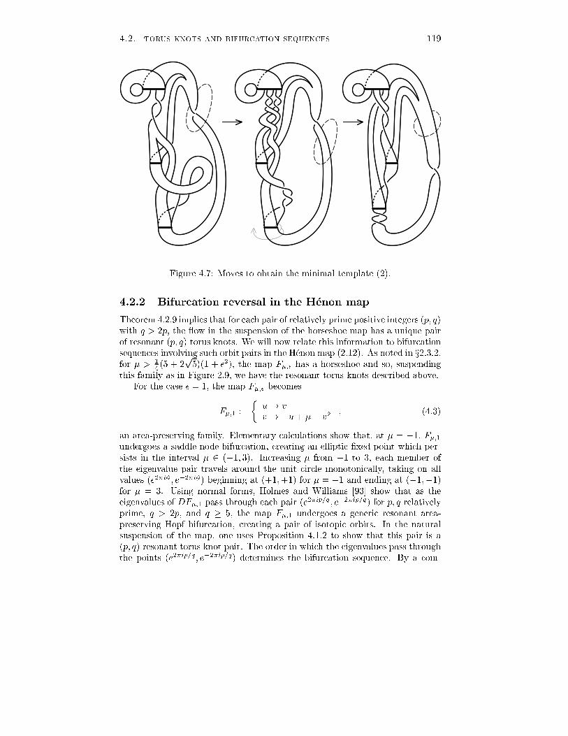
4.2. torus knots and bifurcation sequences 119

Figure 4.7: Moves to obtain the minimal template (2).4.2.2 Bifurcation reversal in the H�enon mapTheorem 4.2.9 implies that for each pair of relatively prime positive integers (p; q)with q > 2p, the ow in the suspension of the horseshoe map has a unique pairof resonant (p; q) torus knots. We will now relate this information to bifurcationsequences involving such orbit pairs in the H�enon map (2.12). As noted in x2.3.2,for � > 14 (5 + 2p5)(1 + �2), the map F�;� has a horseshoe and so, suspendingthis family as in Figure 2.9, we have the resonant torus knots described above.For the case � = 1, the map F�;� becomesF�;1 : � u 7! vv 7! �u+ �� v2 ; (4.3)an area-preserving family. Elementary calculations show that, at � = �1, F�;1undergoes a saddle-node bifurcation, creating an elliptic �xed point which per-sists in the interval � 2 (�1; 3). Increasing � from �1 to 3, each member ofthe eigenvalue pair travels around the unit circle monotonically, taking on allvalues (e2�i�; e�2�i�) beginning at (+1;+1) for � = �1 and ending at (�1;�1)for � = 3. Using normal forms, Holmes and Williams [93] show that as theeigenvalues of DF�;1 pass through each pair (e2�ip=q ; e�2�ip=q) for p; q relativelyprime, q > 2p, and q � 5, the map F�;1 undergoes a generic resonant area-preserving Hopf bifurcation, creating a pair of isotopic orbits. In the naturalsuspension of the map, one uses Proposition 4.1.2 to show that this pair is a(p; q) resonant torus knot pair. The order in which the eigenvalues pass throughthe points (e2�ip=q ; e�2�ip=q) determines the bifurcation sequence. By a com-

120 chapter 4. bifurcations

Figure 4.8: Moves to obtain the minimal template (3).plicated argument involving symmetry properties of the map F�;1 and linkingdata on the q-cables themselves, one shows that the resonant bifurcation pair lieon a continuous branch of resonant torus knots which can be followed from thebifurcation point to � arbitrarily large, thus identifying them with the uniqueresonant pair and enabling one to employ the uniqueness part of Theorem 4.2.9to arrive at the following:Proposition 4.2.14 Given the sequence of pairs of relatively prime positiveintegers f(pi; qi)g+1�1 with q > 2p and q � 5 ordered via i < j if and only ifpi=qi < pj=qj, let �1i be the �-value at which the natural suspension of the mapF�;1 creates the unique pair of (pi; qi) resonant torus knots. Then i < j if andonly if �1i < �1j .For the case � = 0, the map F�;� becomesF�;0 : � u 7! vv 7! �� v2 ; (4.4)the dynamics of which immediately collapse to those of the one-dimensionalquadratic map f� : x 7! � � x21 described in x1.2.3. Kneading theory provides

4.3. self-similarity and horseshoe cables 121a complete ordering of the bifurcations of f� via the kneading invariants �(w).Here the continuation with increasing � of orbits once created is assured bythe monotonicity of the kneading invariant. One uses the algorithm given asExample 4.2.10 of x4.2.1 to construct the words corresponding to such (p; q) res-onant torus partners. Computing the associated kneading invariants (via (1.24)),Proposition 1.2.48 allows us to order these resonant torus pair bifurcations. Thisyields:Proposition 4.2.15 Given the sequence of pairs of relatively prime positiveintegers f(pi; qi)g+1�1 with q � 2p ordered via i < j if and only if pi=qi < pj=qj ,let �0i be the �-value at which the natural suspension of the map F�;0 creates theunique pair of (pi; qi) resonant torus knots. Then i < j if and only if �0i > �0j .We note that the kneading theory behind Proposition 4.2.15 applies to anyunimodal function of v in place of �� v2 in F�;0. Thus, the conclusion holds fora far wider class of mappings than the H�enon family.These propositions together imply the following remarkable result [93, 87]:Theorem 4.2.16 (Holmes and Williams [93]) In the bifurcation diagram of themap F�;�, in�nitely many saddle-node bifurcation curves cross one another onthe (�; �) parameter plane between � = 0 and � = 1. In particular, each resonanttorus bifurcation sequence for the area-preserving case (� = 1) is exactly reversedin the one-dimensional case (� = 0).Thus, �xing � 2 [0; 1], and increasing �, we obtain in�nitely many di�erentbifurcation sequences leading to a horseshoe: loosely speaking { in�nitely manyroutes to chaos. However, this behavior does not imply similar reversals forother orbits. For example, the (2,3) non-resonant torus knots of periods 4,5,6: : :do not reverse their order in this way; instead, as an accumulating family of thetype described in Theorem 3.1.20, their bifurcation curves are all \parallel:" cf.Holmes and Whitley [92].4.3 Self-similarity and horseshoe cablesGiven the correspondence between knotted orbits on the horseshoe template andbifurcations of the one-dimensional quadratic family touched on in x4.2, we nowexplore this latter family of maps in greater detail.Denote by f� the map which takes x to �� x21, where f� acts on the inter-val I(�) = h� 12 �q�+ 14 ; 12 +q�+ 14i (this interval grows as � ranges over[� 14 ; 2]). The bifurcation set of this map has a remarkable self-similar struc-ture: given any positive integer M , there exists at least one subset J , of thephase-parameter space for which fM� ��J � f�; (4.5)

122 chapter 4. bifurcationswhere � denotes conjugacy. Figure 4.9 illustrates the case M = 3: f3� restrictedto a subinterval [�; �] has the same bifurcation sequence on some ��subintervalas does f� on [� 14 ; 2]). This is the basis for a renormalization group theory (see[95, 96]) which shows that bifurcation sequences are nested within themselves.The simplest such nesting leads to the well-known period-doubling cascadesstudied metrically by Feigenbaum and others (see [41, 199]).

Figure 4.9: f3� and a magni�cation.Orbits in the quadratic map are created in a very speci�c order, governedby the kneading invariants (Proposition 1.2.48). As we have seen in x4.2.2, ahorseshoe may be \built" through a variety of distinct paths; nevertheless, bytaking the branch line of H as a Poincar�e section for the semi ow, we recover the\full" quadratic map as a return map. Thus, as per Remark 4.2.6, we may speakof two horseshoe knots being a saddle-node pair, based on the correspondingtheory for the one-dimensional return map.In this section, we explore the implications of the bifurcation structureswithin f� on knot and link types and on subtemplate structures within thetemplate H. We �rst outline an extension to the simple kneading theory intro-duced in x1.2.3, and use it to show how certain classes of words correspond toknots inhabiting subtemplates of H. This material is drawn from [88], in whichthe idea of subtemplates �rst appeared, but the proof of the main result (The-orem 4.3.8) is reformulated and simpli�ed in terms of the template in ationsintroduced in Chapter 2.4.3.1 Kneading factorization and subtemplatesThe kneading invariant introduced in x1.2.3 provides a convenient symbolic toolfor analyzing iterated structures on the template. For the horseshoe template,the kneading invariant �(a1) of a periodic orbit a1 is a sequence given by (1.24)which, via Proposition 1.2.48, allows one to order the �-values at which the orbitsappear in bifurcations of the one-dimensional map f�. In cases where �(a) isperiodic, we refer to it by the periodically repeated unit, with the superscript 1dropped.

4.3. self-similarity and horseshoe cables 123We now describe a factorization of such kneading sequences.De�nition 4.3.1 For w an acyclic minimal word w = w1w2 : : : wk and v anyword v = v1v2 : : : (not necessarily �nite), de�ne w � v to be the sequence ofconcatenated words w � v = wv1wv2wv3 : : : (4.6)where wx1 = w = w1w2 : : : wkand wx2 = w = w1w2 : : : wk :Recall from x1.2.3 that x1 = x2 and vice versa.Example 4.3.2x1x2 � x1x1x2 = x1x2 x1x2 x2x1= x1x2x1x22x1x1x2 � x1x2x2 = x1x2 x2x1 x2x1= x1x22x1x2x1x1x1x2 � x1x2x1x1x2 : : : = x1x1x2 x2x2x1 x1x1x2 x1x1x2 x2x2x1 : : :Any kneading invariant � which can be expressed as a �-product of two ormore nonempty words is said to be �-factorizable, otherwise it is �-prime. The �-factorization is particularly useful in describing period multiplying bifurcations.For example, in the period-doubling bifurcation of a period-k orbit with periodickneading invariantw, the new orbit of period 2k has kneading invariantw�x1x2.The �-products can be iterated to form longer, more complicated factorizations.The self-similarity for the quadratic map f� in (4.5) is naturally expressedin terms of kneading sequences and �-factorization (see [88]):Lemma 4.3.3 Let u;v and w be kneading invariants, where w is �nite. Thenw � u�w � v if and only if u� v.Proof: By Equation (4.6), w � u = wu1wu2 : : :w � v = wv1wv2 : : : :Let K denote the index of the �rst letter at which u and v di�er; hence,uK = x1; vK = x2. Since w is a kneading invariant, it follows from (1.24)that w1 = x1. Thus, wuK �wvK and w � u � w � v. Reversing the argumentyields the lemma. 2Remark 4.3.4 In conjunction with Proposition 1.2.48 and Equation (1.24),Lemma 4.3.3 implies the self-similarity in the bifurcation structure stated inEquation (4.5). Increasing � creates periodic orbits in the order of increasing �

124 chapter 4. bifurcationsfrom x11 to (x1x2)1, to (x1x2)�(x1x2), etc., ad in�nitum. For any �nite �-primekneading words u�v, all kneading sequences of the form u �w, for all w, mustpreceed v; hence, the entire bifurcation sequence of f� is \embedded" withinitself, so that fM� restricted to some subinterval in � undergoes the \same"sequence as f� itself.Recall from De�nition 4.2.5 that male knots have even x2-parity and femaleknots, odd x2-parity. The kneading theory for unimodal maps implies thatmales are created in saddle-node bifurcations and females in either saddle-nodes(along with males) or, partnerless, in period-doubling bifurcations. Directlyafter either such bifurcation, both orbits implicated in it share the same symbolsequence. After the saddle node, that destined to become female changes gendervia one point on it crossing the critical point c; the male's sequence remains asit began, consistent with a positive eigenvalue. After a q ! 2q period doubling,the doubled orbit, whose sequence, regarded as 2q-periodic, starts out male,similarly changes gender by losing or gaining an x2 as a point of it passes c.(Recall that the eigenvalue of the (iterated) maps are respectively 1 and �1 inthese bifurcations.) These observations imply the following (for details see [88]):Lemma 4.3.5 Let w be a q-periodic kneading invariant. Corresponding to wand w � x1x2, there exist two horseshoe periodic orbits, (a0)1 and (a)1 2 �H,such that:1. w = �((a)1) = �((a0)1);2. if w 6= u � x1x2 for any kneading invariant u, then (a0)1 and (a)1 are amale-female pair of isotopic period-q orbits created in a saddle-node bifur-cation;3. if w = u � x1x2 for some kneading invariant u, then (a0)1 and (a)1 areboth female knots implicated in a period-doubling bifurcation and havingrespective periods q and 2q.De�nition 4.3.6 Let fwign1 denote a collection of qi-periodic kneading invari-ants for some n > 1, and W = w1 �w2 � � � � �wn be the Q = Qni=1 qi-periodickneading invariant formed by iterated �-multiplication. A periodic horseshoe or-bit (a)1 having kneading invariant �((a)1) =W is called an iterated horseshoeknot with de�ning sequence W .The factorization of kneading invariants becomes the dynamical backbone foran elegant interpretation of self-similarity in the bifurcations of the horseshoe.The topological analogue of the �-factorization is a generalization of the satellite-companion construction for knots (De�nition 1.1.10):De�nition 4.3.7 Let T be a template braided within a standardly embeddedsolid torus V = D2 � S1, and let K be a knot (in a di�erent copy of S3) withtubular neighborhood N(K) homeomorphic to V via h : V ! N(K). Then thetemplate given by h(T ) is a satellite of T with companion K.

4.3. self-similarity and horseshoe cables 125Theorem 4.3.8 (cf. Holmes [88]) Let W = w1 � w2 � � � � � wn be a periodickneading invariant which does not factor as u � (x1x2) for any kneading invari-ant u. Also, denote by (a0)1 and (a)1 2 �H the male-female pair of knotsassociated to W via Lemma 4.3.5. Then, all the iterated horseshoe knots of theform W �v coincide with the closed orbits on a particular subtemplate HW � Hwhich is the satellite of either the standard horseshoe template H or the \twisted"horseshoe template ~H (pictured in Figure 4.10), with the knot corresponding to(a)1 as companion.x1 x2

Figure 4.10: The \twisted" horseshoe template ~H.Proof: Let (a0)1 be the (Q-periodic) itinerary of the male horseshoe knot havingkneading invariant �((a0)1) = W and let (a)1 correspond to the female knothaving kneading invariant �((a)1) =W � x1x2 as per Lemma 4.3.5. Denote byb be the subword a1a2 : : : aQ�2 of a (or, equivalently, a0).Assume �rst that b has odd x2-parity; then, consider the in ationEW : H ,! H � x1 7! x2bx1x2 7! x2bx2 : (4.7)The image of this map is a template since E preserves the twist orientation of

126 chapter 4. bifurcationsx11 and x12 , and since the image of the branch segments,�1(EW(H)) = EW([x11 ; x1x2x11 ])= [((x2bx1))1 ; x2bx1x2bx2 (x2bx1)1];�2(EW(H)) = EW([(x2)2x11 ; x2x11 ])= [(x2bx2)2 (x2bx1)1 ; x2bx2 (x2bx1)1]: ; (4.8)is a set of nonoverlapping intervals on the branch line (this may be veri�ed usingthe �-ordering and the fact that b is of odd x2-parity).By Lemma 4.3.5, the knots corresponding to (a)1 and (a0)1 on H are iso-topic: the isotopy is merely that of Lemma 4.2.3 | the rightmost strand of theknot for (a0)1 on the x1 strip of H is lifted over the branch line gap to theleftmost strand of the knot for (a)1 on the x2 strip. Since the periodic orbits(a)1 and (a0)1 form a \spine" for the subtemplate E(H), the isotopy may beextended to the strip containing (a0)1. Hence, the subtemplate E(H) may beisotoped in S3 to lie within a tubular neighborhood of the knot correspondingto (a)1. This yields a presentation of HN = E(H) as a satellite template withcompanion (a)1.To show that HN contains precisely the iterated horseshoe knots, observethat W and W �x1x12 are respectively the smallest and largest kneading invari-ants of the form W � v for any v. Hence, all orbits with kneading invariantsof this form must lie between the horseshoe words having kneading invariantsW and W � x1x12 . But these correspond precisely to the boundary componentsE(x11 ) and E(x2x11 ) of the subtemplate.In the case where the x2-parity of b is even, we must modify the in ation Eto one which respects even and odd twisting of orbits. An analogous proof tothat above, applied to the in ation~EW : ~H ,! ~H � x1 7! x2bx2x2 7! x2bx1 ; (4.9)shows that the subtemplate containing the iterated horseshoe knots is a satelliteof the \twisted" horseshoe template ~H. 2Example 4.3.9 Let W = x1x32x1, so that a0 = x1(x1x2)2 and a = x21x32. Thein ation is: Ex1x32x1 : H ,! H � x1 7! x2(x21x2)x1x2 7! x2(x21x2)x2 :Figure 4.11 shows that, after an isotopy, HN is a satellite of H with companiona trefoil, having an additional four full twists.Similarly, the net twisting for HN with W = x1x22x1x2 is odd. RecallingExample 4.2.2, the reader may like to check that this subtemplate is a satelliteof the twisted horseshoe ~H with companion a (2; 5) torus knot, having four andone-half full twists.

4.3. self-similarity and horseshoe cables 127

Figure 4.11: the subtemplate for W = x1x32x1. (a0)1 is shown solid, (a)1dashed.In this sense, the male-female pair (a0)1 ; (a)1 give rise to a family of iteratedhorseshoe knots which remain close to them in that they lie on the subtemplateHN . We refer to (a0)1 and (a)1 as the father and mother knots respectively;the iterated knots are their children. From Theorem 4.3.8, we observe that (a)1can be viewed as the core of an embedded torus, with (a0)1 on its boundary andall subsequent children following (a)1 without doubling back. Hence, iteratedhorseshoe knots are examples of the generalized cablings discussed in x1.1.2.4.3.2 Nested periodic orbits and iterated torus knotsThe self-similarity in the bifurcation structure of the quadratic family is not theonly example of dynamical self-similarity. A very important and well-knownclass of examples is given in the KAM theory for elliptic �xed points of anarea-preserving di�eomorphism [122, 123]. Let F : R2 ! R2 and DF (�) haveeigenvalues �; � = e�2�i� with � 2 (0; 12 ). Generically F is a perturbed twistmap with rings of alternating elliptic and hyperbolic points arranged in a self-similar fashion. These families of periodic points are separated by invariant\KAM curves," which form a set of positive Lebesgue measure; see [8].There is much to be said concerning the knotting and linking of orbits in

128 chapter 4. bifurcationsthe suspension of such a map, or, more generally, for any Hamiltonian ow on aconstant-energy three-manifold (see, e.g.[116, 15]). In particular, since the area-preserving H�enon map provides a speci�c example of such a map, we shouldexpect to see some vestige of this behaviour in the horseshoe.We showed in x4.2.2 that, around the \primary" elliptic point, correspondingto the (female) orbit x2, the natural suspension of the area-preserving H�enonmap has a (p; q) torus knot pair for each p < q=2. In fact, much more is true:the self-similar structure suggested in the KAM Theorem corresponds, in thesuspended ow, to iterated torus knots of in�nitely many (but not all) types.The simplest of these are the 2-cables created in period doubling sequences, asexpressed in the following simple corollary to Lemma 4.3.5:Corollary 4.3.10 All female horseshoe knots are 2-cabled by some other horse-shoe knot.Proof: Let (a)1 denote the itinerary of the female horseshoe knot. Then, theperiodic orbit corresponding to the kneading invariant �(a) � x1x2 is a 2-cableof (a)1 by Lemma 4.3.5 and Proposition 4.1.2. 2Remark 4.3.11 Since any periodic orbit with kneading invariant of the formw � x1x2 is female, and those orbits created in the period doubling sequencebased on the (female) orbit (a)1 with kneading invariant w have invariants w �x1x2; w�x1x2�x1x2; : : : , any �nite part of every period doubling sequence formsan iterated 2-cable of (a)1. Formulae describing crossing and linking numbersof such structures may be derived. For example, see [88] for a presentation ofthe period-doubling cascade results of Yorke and Alligood [198, 199] in knot-theoretic terms.We now move to more general iterated torus knots. To proceed, recall the no-tion of type numbers following De�nition 1.1.10. We call an iterated (horseshoe)torus knot of type f(p1; qi)g (with pi < qi; 8i) resonant if its type numbers qicoincide with the periods qi of the kneading invariantswi in its de�ning sequenceW .Theorem 4.3.12 (Holmes [88]) Among the iterated horseshoe knots, each �nitesequence f(pi; qi)gn1 of positive integers with pi; qi relatively prime and pi=qi < 12determines a unique pair of resonant iterated torus knots of type f(bi; qi)gn1 whereb1 = p1 and bi+1 = qi+1qibi + (�1)ipi+1: (4.10)This result is essentially an iterated version of Theorem 4.2.9. It is proved byidentifying the appropriate iterated horseshoe knots via their words and factoredkneading invariants, and placing them correctly on the subtemplates of Theorem4.3.8. The words are �-multiplied analogues of those for the simple torus knotsof Theorem 4.2.9, and uniqueness follows by alternately maximizing and mini-mizing crossing numbers and appealing to Theorems 2.2.4 and 4.2.8. (Here, the

4.4. homoclinic bifurcations 129embedded subtemplates are suÆciently twisted for one to apply Theorem 4.2.8directly; no elaborate surgery as in Figure 4.6 is required.) The argument islengthy and not particularly illuminating; for details and data on the associatedkneading invariants and linking numbers see [88].We close with a summary of orbit genealogies for the natural suspension ofthe horseshoe map. Generically, orbits appear as male-female pairs in saddle-node bifurcations, or as single female knots in period-doubling bifurcations. Thefemale knots are \mothers," each of which forms the core of a subtemplate hav-ing the associated \father" knot as a boundary component. The mother isa companion (in the sense of De�nition 1.1.10) to her in�nitely many \chil-dren:" generalized cables which live on her subtemplate. Approximately halfof these knots are female, and as such, proceed to form sub-subtemplates sup-porting in�nitely many grandchildren, etc. Since each subtemplate is a twistedand (perhaps) knotted copy of the original, the bifurcation sequences on eachsubtemplate are miniature copies of the original but yield knots increasing incomplexity. Not only are the individual orbits knotted and linked, but the sub-templates containing certain lineages of orbits are also twisted and linked aboutone another.4.4 Homoclinic bifurcationsWe now turn to some knot and link structures associated with global bifurcationsinvolving homoclinic orbits to hyperbolic saddle points in three dimensional ows: _x = f(x): (4.11)Suppose the saddle point lies at x = 0 (f(x) = 0) and let �i denote the eigen-values of the linearization Df(0). There are many possible cases to consider,for real and/or complex eigenvalues, and expanding or contracting ows, and weshall only give a brief sample of results. We start with the real, contracting case,summarising some results from [91], which the reader should consult for furtherdetail.4.4.1 Gluing and torus knotsSuppose that Df(0) has three real eigenvalues with the single expanding eigen-value �u > 0 weaker in magnitude than the two contracting eigenvalues: ��ss >��s > �u > 0. We assume that both branches of the one-dimensional unstablemanifoldW u(0) lie in the two-dimensional stable manifoldW s(0) and denote by� the set W u(0)[ f0g. This is a codmension two bifurcation, generically occur-ring at isolated points in parameter space for a two-parameter family of vector�elds f(x;�1; �2) (i.e., no symmetries are present). Letting (�1; �2) = (0; 0) besuch a point and varying (�1; �2), the degenerate case unfolds to the gluing bifur-cation, in which up to two periodic orbits bifurcate from the double homoclinicloop � [63, 72].

130 chapter 4. bifurcationsBefore stating the principal result, we must develop a little machinery. De-note the two loops of �: x1 and x2. The bifurcating periodic orbits may followx1 and/or x2 many times before closing, giving a natural description as a word,much as in the symbolic description of templates. Those words which actuallyoccur determine the unfolding. [63, 72] prove that any periodic orbit bifurcatingfrom � must have a rotation compatible word.De�nition 4.4.1 An in�nite (�nite) word in two symbols is rotation compatibleif it can be represented as the (�nite periodic) itinerary of an orbit of a rigidrotation map �� : z 7! (z + �), z 2 S1, with the Markov partition I(x1) =(0; 1� �], I(x2) = (1� �; 1] for some � 2 [0; 1). The unique � for such a word isits rotation number .Remark 4.4.2 To compute the rotation number of a given �nite rotation com-patible word, take the number of x2's and divide by the total length of theword: e.g., x21x2x1x2 ) � = 25 . The rotation compatible words are precisely the\evenly distributed" words of Theorem 4.2.9. Finally, we recall that two rationalnumbers pq and p0q0 are Farey neighbors if j pq0 � qp0 j= 1.Theorem 4.4.3 (Coullet et al. [63, 72]) For every suÆciently C1-small pertur-bation of f(x; 0; 0) there are at most two periodic orbits in a small neighborhoodN of �. Any such periodic orbits are attracting and have rotation compatiblewords, and, if there are two, their rotation numbers are Farey neighbors.The proof uses the eigenvalue condition, which implies that a small neighbor-hood of � is positively invariant and so contains an attractor, even after (small)perturbation. De�ning cross sections near 0, one shows that the resulting returnmap is a (discontinuous) contraction. This, together with the fact that the at-tractor lies within the closure of the one-dimensional unstable manifold W u(0),of which there are two branches, implies that there are at most two stable pe-riodic orbits for any given parameter pair (�1; �2). The admissible words areconstructed via a reduced (one-dimensional) return map, which is e�ectively adiscontinuous mapping of the circle. Note that there may be two, one, or noperiodic orbits: both branches of the unstable manifold may limit on an \irra-tional" curve which winds repeatedly about, never closing.Thus, unlike the expanding Lorenz ow, which is also related to a doublehomoclinic connection, gluing bifurcations create isolated periodic orbits char-acteristic of Morse-Smale ows (cf. Appendix A). The interest here is in de-scribing how the rotation compatible periodic orbits succeed one another as theparameters (�1; �2) vary, and which knots and links they form. To determinethe latter we will construct \templates" for the ows, relaxing the expansivenessdemanded by the de�nitions of x2.2 to include contracting ows.There are two distinct topological con�gurations, depending upon which sidesof W s(0) the homoclinic orbits reenter: these are the �gure-of-eight and thebutter y, shown in Figure 4.12. For both systems, we assume the existence

4.4. homoclinic bifurcations 131of a strong stable foliation (reported in [72] to be a generic condition in thesecases) and collapse out as in the proof of Lemma 2.2.7, leaving a (contracting)template. Alternatively, these branched manifolds may be viewed as embeddedsuspensions of one-dimensional noninvertiable return maps.

(a) (b)Figure 4.12: (a) The �gure-of-eight and butter y con�gurations, and (b) asso-ciated templates.Embedding these templates in R3, we must incorporate the \twist" of the ow around the homoclinic connections, which leads to twisting of the templatestrips. Temporarily ignoring full (even) twisting of each strip and excludingnon-trivially knotted embeddings, there are three intrinsic cases to consider:untwisted : �1 = �2 = 0; singly-twisted : �1 = 0; �2 = 1; and doubly-twisted :�1 = �2 = 1, also illustrated in Figure 4.12. Below we give results only for thebutter y case: the �gure-of-eight, whose template is unbranched, is somewhatsimpler. For details see [91].Case (1) untwisted: �1 = 0; �2 = 0Using the theory of circle maps (one views the Poincar�e map as a monotoneinjective map of the circle with a single discontinuity), in [72, 65], it is provedthat this system has at most one periodic orbit. As an addendum to this, wehave:

132 chapter 4. bifurcationsProposition 4.4.4 Any periodic orbit appearing in the unfolding of an un-twisted butter y is a torus knot. If the rotation number of the word is � = pq+p ,then the corresponding knot type is (p; q).Proof: Note that, although the dynamics of the contracting butter y systemdi�er greatly from that of the expanding Lorenz ow, the associated templatesare isotopic, and their labeling by x1; x2 consistent. We shall extract a subsetcontaining the given rotation compatible word from the Lorenz template L(0; 0)and show that it embeds in a torus. This, together with Theorem 4.4.3, provesthe claim, and also proves the last statement in Theorem 2.3.3.Pick a word with p x1's and q x2's and assume that p > q (If q > p, ipL(0; 0) about the vertical axis and proceed by symmetry). Then, since the wordis evenly distributed, there are no consecutive x2's and each trip about the x2-strip is immediately followed by a trip about the x1-strip. The orbit in questiontherefore lies on an unbranched subset S � L(0; 0) that may be isotoped as in-dicated in Figure 4.13, from which it is clear that it winds p times longitudinallyand q times meridionally around a torus T 2. (For this case �1 = 0, but note forlater use that one can make the same isotopy moves, simply carrying the �1 halftwists along, since the split does not extend that far.) 2

p� q qp p� qqFigure 4.13: The subset S � L(0; 0) �ts on a torus T 2. The labels refer to thenumber of strands on each strip.Example 4.4.5 The words x21x2x1x2 and x1x22x1x32 correspond to (2; 3) and(5; 7) torus knots respectively. Note that the mapping from words to torusknots di�ers from that on the horseshoe template H = L(0; 1), described in theproof of Theorem 4.2.9.

4.4. homoclinic bifurcations 133Observe that this result merely proves that if an orbit with the given wordexists, then it is a torus knot of the type speci�ed. To �nd such orbits, one hasto tune the parameters (�1; �2) appropriately, as speci�ed in the bifurcation di-agrams of [72, 65] and summarised in [91]. Between each pair of (disjoint) opensets (�1; �2) giving rise to torus knots of Farey neighbor types (p; q), (p0; q0) ,there is a set having knots of type (p+p0; q+q0): the Farey mediant. In this way,passing across the parameter plane, one exhausts all torus knots. Intuitively, weare moving the thin incoming strips along the branch line of the contractingtemplate to match up, one by one, the \ends" of the torus knots which all co-exist on the expanding Lorenz template L(0; 0).We brie y consider the impact of introducing �1 (even) positive half-twistsalong the x1 branch. The proof of Proposition 4.4.4 may be modi�ed to copewith this case, as already indicated. Even if �1 is non-zero we may perform thesame moves without interference from the additional half-twists. Then, since �1is even and there are 12�1 full twists, we obtain a (p; q + 12p�1) torus knot (tocheck this, refer to the positive braid genus formula of Equation (1.4)). A similarargument for �1 = 0 and �2 even yields a (p+ 12q�2; q) torus knot.If both �1 and �2 are simultaneously non-zero and even, the resulting subsetS can still be presented as a positive braid on p strands, but it is no longera torus knot, for there is additional twisting on the strip carrying q strands.Indeed, it does not appear to belong to any well-known knot family. A pictureand genus formulae for this case appear in [91].Case (2) singly- and doubly-twisted: �1 = 0; 1; �2 = 1In these cases one can use contraction and orientation-reversal properties ofthe one-dimensional return map induced by the semi ow, along with templatesurgery analogous to that of Figure 4.13, to prove the following rather restrictiveresult:Proposition 4.4.6 ([91]) If the x2-branch of the butter y template has a half-twist (case (2)) then all periodic orbits appearing on it must have words x1 orxk1x2 (k � 0). The same holds reversing x1 and x2. If both branches have halftwists (case (3)), then only x1, x2, and x1x2 may appear. Any periodic orbitappearing in the unfolding of either case is an unknot.Remark 4.4.7 The signi�cance in the knotting and linking of orbits implicatedin gluing bifurcations lies not so much in extracting bifurcation invariants (forthese bifurcations are fairly well-understood), but in displaying the general prin-ciple that simple dynamics are coupled with the existence of simple knots andlinks. The fact that only torus knots can occur in a butter y-gluing bifurcation(in which the ows are all zero-entropy) is in stark contrast to the analogouspositive entropy Lorenz ow, in which an in�nite array of knot types coexist: cf.Theorems 3.1.15 and A.1.13.The next example of global bifurcations exhibits an opposite extreme of topo-logical complexity.

134 chapter 4. bifurcations4.4.2 Silnikov connections and universal templatesWe now return to the example presented in x2.3.3: a radically di�erent type ofglobal bifurcation, originally studied by Shil'nikov [160, 161] (cf. [179] and thetextbooks [76, 188, 189], which also contain these and related results). The ma-terial below is adapted from [71]. Recall the de�nition of a Shil'nikov connection,De�nition 2.3.8, and the associated Theorem 2.3.9: that a countable collection ofsuspended horseshoes lives in a tubular neighborhood of a Shil'nikov connection.Sketch of proof of Theorem 2.3.9: We construct Poincar�e sections transver-sal to � near the �xed point p and linearize the ow near p and along � toobtain approximate return maps. The horseshoes are constructed by owingpairs of boxes near p and then along �. The �xed point has a one-dimensionalunstable manifold W u(p) and a two-dimensional stable manifold W s(p), alongwhich � =W s(p)\W u(p) spirals into p. (Although we consider only the case inwhich W u(p) is one-dimensional, our results apply equally well to W u(p) two-dimensional andW s(p) one-dimensional, since this amounts to a reversal of timewhich leaves periodic orbits invariant.)

��0�1

W s(p)�1

�0 �+0

Figure 4.14: Cross sections and maps near the �xed point p.We construct Poincar�e sections �0 and �1 transverse to � and suÆcientlyclose to p that linear analysis provides a good estimate of the return map. Thesurface �0 is bisected by W s(p) into upper (�+0 ) and lower (��0 ) halves. We usea cylindrical coordinate system having origin at p and with �0 at constant r and�1 at constant z = �� 1 (this is the convention of [76] | one may just as well

4.4. homoclinic bifurcations 135choose �0 at constant � [74, 189]): see Figure 4.14. The return map factors intothe \local" map �0 : �+0 ! �1, which is concentrated near p, and the \global"map �1 : �1 ! �0, which follows orbits along near �. Hypotheses (1) and (2)permit us to construct approximations to these maps.Taking �0 and �1 close enough to p, the ow linearised at p,r(t) = r0e��st�(t) = �0 + !t (4.12)z(t) = z0e�ut;provides a good approximation of �0. Solving z(T ) = � for T , we obtain thetransit time for orbits leaving �0 to reach �1:T (z) = 1�u log �z : (4.13)This yields an expression for the local return map �0:�0 : (r0; �; z) 7! �r0 � �z��s=�u ; � + !�u log� �z� ; �� : (4.14)Restricting to a suÆciently small neighborhood of � \ �1, one can assumethat the global return map �1 is aÆne. This yields an analytical approximationto the Poincar�e map given by composition of (4.14) with an aÆne map. Suchcomposed maps have been analyzed repeatedly [160, 161, 74, 66].The action of �0 on a segment of constant � is to stretch it and wrap it around� \�1 in a logarithmic spiral. Since z = 0 is on W s(p), the image of �0(r; z) asz ! 0 approaches � \�1. This image is then mapped aÆnely back to �0, with�1(� \�1) = � \ �0: see Figure 4.14.One now examines the action of �1�0 on rectangular strips:Bi = f(�; z) � �+0 : ai � z � big; (4.15)where the sequences faig and fbig satisfy ai < bi < ai�1 and limi!1 ai = 0. Forappropriate choice of numbers fai; big, it can be shown [76, 188, 189] that theimage of each adjacent pair fBi [Bi+1g under �1�0 intersects Bi [Bi+1 to forma hyperbolic horseshoe (see e.g. Theorem 4.8.4 of [189]): see Figure 2.11(b).These pairs are the horseshoes of Theorem 2.3.9. 2We now develop a geometric treatment based on the analysis sketched above(cf. [5]), which will allow us to extract the desired templates and prove that the ow in a neighborhood of a double Shil'nikov connection contains representativesof all knots and links.Single Shil'nikov templatesThe horseshoes of Theorem 2.3.9 are hyperbolic, so we may collapse along thestable foliations and, carefully following the embedding, construct the embedded

136 chapter 4. bifurcationstemplate. We proceed in two steps, according to the two components of thereturn map �1�0.First, the action of the global map �1 is aÆne and takes the image under�0 of the \horizontal" Bi � �+0 to a \vertical" strip in �0. Collapsing in thecontracting direction of the map �0�1, each box Bi � �+0 becomes a verticalinterval fai � z � big at a �xed r. Thus, the collapsed Bi and Bi+1 boxes aredisjoint within �+0 . Their images, however, are vertical lines which cover �0;hence, the two strips are joined at a branch line.Since �1 is aÆne, there is no additional folding. Therefore, instead of col-lapsing the stable direction out to obtain a branch line in �+0 , we can propagatethe branch line back via ��11 to depict the joining of these strips within �1, asin Figure 2.12(b). The impact of �1 on the topology of the suspension is en-coded in the twist of � between �1 and �+0 (cf. Remark 1.2.18). For N a smalltubular neighborhood of � excluding a small neighborhood of p, W s(p) \ N isa two-dimensional strip which may twist any number of times about �. Since�1�0(Bi) transversally intersects W s(p), the template inherits this same twist:see again Figure 2.12(b).The action of the local map, �0, is to stretch Bi out along what was thez-direction in �+0 and compress Bi along what was the �-direction. The imageof �0(�+1 ) is a thin spiral (imagine thickening that in Figure 4.14). The image ofany consecutive pair Bi; Bi+1 lies within a folded strip: a horseshoe. As the boxBi � �+1 ows through a neighborhood of p to reach �1, it is wrapped around� an integer number of half-turns, Bi+1 being wrapped with one more half-turnthan Bi. Indeed, the winding which occurs near p is revealed by Eqn. (4.14).As detailed in [188, 189], the boxes Bi can be chosen such thatai = �e��i�u=!: (4.16)Hence, �� � !(T (ai+1)� T (ai)) (4.17)= !�u �log �ai+1 � log �ai� = �;and the action of the ow of Bi+1 from �+0 to �1 is to wind about � in the �direction by an additional �, compared to Bi. This is shown in Figure 4.15.Remark 4.4.8 The strips drawn in Fig. 4.15 are shown with minimal twisting;however, there is no guarantee that the \topmost" Bi, which su�er the leasttwist, satisfy the hyperbolicity conditions necessary for Theorem 2.3.9. We onlyknow that for i (and hence, twist) suÆciently large, pairs of boxes Bi[Bi+1 canbe chosen so that their images form hyperbolic horseshoes.We may now classify the types of horseshoe templates which appear near�. For i some �xed integer, consider the template formed by collapsing thecontracting directions of the ow of the boxes Bi and Bi+1. In a neighborhoodof p, the strip corresponding to Bi (resp. Bi+1) winds about � with i (resp.

4.4. homoclinic bifurcations 137

Figure 4.15: A \simple" Shil'nikov horseshoe.i+1) half-twists. The strips join at �1 in a single strip which follows � back to�0, undergoing a further M half-twists, for some �xed (but unknown) M .If we assume that the homoclinic connection is unknotted, the template thusobtained depends only on the depth of the horseshoe, i, and the �xed globaltwisting, M . Up to homeomorphism, there are two types, depending upon theparity of � � i+M . The template H� is shown in Figure 4.16: for � even, thisis homeomorphic (though not isotopic!) to the standard horseshoe template H(cf. Figure 2.9), and for � odd, this is homeomorphic to the \twisted" horseshoetemplate ~H of Figure 4.10. For any �, H� is isotopic to H with � additionalhalf-twists inserted after the branch line.For a given ow, the global twisting M and the minimum depth i of itshorseshoes are e�ectively uncomputable; hence, one cannot rigorously concludethe existence of any particular H� for a �xed system, only for � greater thansome (unknown) lower bound. We will now bypass this problem by consideringa double connection which induces equal positive and negative twisting andcancelling the two unknown twists.Double Shil'nikov templatesDe�nition 4.4.9 A function f : Rn ! Rn is equivariant with respect to afunction : Rn ! Rn if f(x) = f((x)) for all x 2 Rn.We shall consider Shil'nikov connections in which the vector �eld of thedi�erential equation _x = f(x) is equivariant under a symmetry of one of the

138 chapter 4. bifurcations�

Figure 4.16: The single loop Shil'nikov horseshoe template H�.following forms: : (x; y; z) 7! (�x;�y;�z) : (x; y; z) 7! (�x;�y; z) : (4.18)Such symmetries are quite common: the Lorenz system exhibits the second type[114, 76]. If the system additionally has a �xed point, p, satisfying the condi-tions of Theorem 2.3.9, the ow will appear as one of the three cases shown inFigure 4.17, displaying either a pair of homoclinic spirals at p = (p), or a spiralheteroclinic cycle connecting p and (p) 6= p. Naturally, an analogue to Theo-rem 2.3.9 holds in this case, with the added ingredient of \coupled horseshoes"[75, 86, 16].We now extend the arguments given above for the single loop case to thedouble loop homoclinic orbit of Figure 4.17 [left], having the �rst symmetryof equation (4.18), so that the loop � has a partner �0 = (�). (The otherheteroclinic cases can be dealt with similarly: see [71] for details.) As in thesingle loop case of Figure 4.14, we de�ne Poincar�e sections �0 and �1, but nowalong with their images under : �00 and �01. Note that �1 is above the saddleand �01 below, and �0 and �00 on opposite sides. Using the same linear andaÆne approximations as before, we derive two local and two global return maps�0 and � 00 and �1 and � 01, but in this case we de�ne strips Bi � �0 and B0i � �00,so that �0(Bi) � �0, � 00(B0i) � �00, �1(�1) � �00 and � 01(�01) � �0. Thus werestrict our attention to orbits which make double traverses of a neighborhoodof � [ �0, tracking the two loops in regular succession.Following the construction for the single loop case, we produce the templateof Figure 4.18, in which the strip leaving the upper branch line in �1 connects to�00, and that leaving the lower branch line in �01 connects to �0. The resulting

4.4. homoclinic bifurcations 139

Figure 4.17: Three symmetric homoclinic con�gurations.template has two branch lines and contains a copy of the single loop templateH� of Figure 4.16 followed by its image under . Since reverses orientation(det(D = �1)), the sense of twist in these two components is opposite; indeed,whatever the depth i, we may collect all the \extra" twisting of the upper com-ponent as a group of � = i +M positive half twists and that of the lower as� negative half twists. These twists may clearly be cancelled exactly, leaving apair of \simple" horseshoe templates, one positive and one negative, as shownin Figure 4.18. We call the resulting template Z .Remark 4.4.10 We assume that the homoclinic/heteroclinic connections in-volved in the double Shil'nikov connection are unknotted. Otherwise, the tem-plate Z might be nontrivially knotted, obstructing our �nal step below.ODEs which generate all knots and linksThe template Z , which appears near the double Shil'nikov loop, shares therichenss of the templates of x3.2:Lemma 4.4.11 The template Z is universal: it contains an isotopic copy ofevery knot and link.Proof: The symbolic in ation I given byI : V ,! Z 8>><>>: x1 7! x2x4x2 7! x1x3 7! x4x2x4 7! x3 ; (4.19)de�nes a map from V into Z . The astute reader will note that the images ofthe periodic orbits (x1)1 and (x3)1 2 V map to (x2x4)1 = (x4x2)1 in Z : the

140 chapter 4. bifurcationsx1 x2x3 x4

+���

Figure 4.18: The double loop Shil'nikov horseshoe template Z , before (left) andafter (right) cancelling the opposite twists.same orbit. While this precludes Equation (4.19) from satisfying the de�nitionof an in ation (the image is not a proper subtemplate), we may neverthelessdisregard this anomaly by performing a DA-splitting of Z along (x2x4)1 andproceeding as usual. The orbit (x2x4)1 is an unknot and there are many moreunknots in the template. Figure 4.19 shows that the subtemplate de�ned by Iis isotopic to V . 2As a corollary, we obtain the following remarkable:Theorem 4.4.12 SuÆcient conditions for a third-order ODE to contain peri-odic orbits representing all knot and link types are that the vector �eld is suÆ-ciently C1-close to a vector �eld satisfying the following four conditions:1. There exists a �xed point p for the vector �eld, and the linearization Df jpat p has eigenvalues f��s � !i; �ug, with�u > �s > 0 ! 6= 0: (4.20)2. The ow �t is equivariant under one of the following symmetries: : (x; y; z) 7! (�x;�y;�z) : (x; y; z) 7! (�x;�y; z) : (4.21)3. There exists an orbit �(t) with limt!�1 �(t) = p and limt!1 �(t) = (p).

4.4. homoclinic bifurcations 141

Figure 4.19: V is a subtemplate of Z .4. The homoclinic/heteroclinic loop(s) is(are) unknotted.The constructions preceeding the proof of Theorem 4.4.12 above actuallyshow that, as one approaches the degenerate double loop, one can pick succes-sively smaller tubular neighborhoods of the double loop which contain in�nitelymany copies of representatives of every knot and link equivalence class.Thanks to the work of Chua et al. [38], we can even display an explicitexample of a three-dimensional system which contains a universal template:Corollary 4.4.13 There exists an open set of parameters � 2 [6:5; 10:5] forwhich the set of periodic solutions to the di�erential equation_x = 7[y � �(x)];_y = x� y + z;

142 chapter 4. bifurcations_z = ��y; (4.22)�(x) = 27x� 314 [jx+ 1j � jx� 1j] ;contains representatives from every knot and link equivalence class.Proof: In [38], it is shown that equation (4.22) satis�es the requirements ofTheorem 2.3.9 for the parameter � in the range indicated. (While this systemis piecewise linear, the construction of the hyperbolic set avoids points at whichthe derivatives are not de�ned, much as the classical construction of Smale'shorseshoe in Example 1.2.28 excludes orbits which enter the preimage of thebend, where the map is strongly nonlinear.) Moreover, the homoclinic connec-tions are both unknotted. A symmetry of the �rst type (4.18) clearly holds forEquation (4.22), so that the template Z is embedded in the ow. Lemma 4.4.11then yields the conclusion. 2Remark 4.4.14 For parameter values of � suÆciently small, the ow given byEquation (4.22) has periodic orbit set consisting of two (symmetric) unknottedseparable attractors. Hence, increasing the parameter � gives a bifurcation se-quence which builds all knots and links from these two \seeds." In contrast tothe H�enon maps of x4.2.2, very little is known about the ordering of bifurcationsand knot types in this sequence.Having given examples in this chapter of knot and link structures which arisein speci�c ows and the templates associated with them, we now return to moregeneral questions regarding templates themselves, viewed in isolation from theirconnections to di�erential equations.

Chapter 5: InvariantsRecall the fundamental problem in knot theory: when are two knots (links)equivalent? An analogous problem presents itself: when are two templates equiv-alent? We must �rst, however, carefully state what equivalence we want, sincewe are chie y interested in the knots and links that inhabit a template, as op-posed to the branched manifold itself. With this is mind, we proceed with asuitable de�nition of equivalence.Recall that many orbits in a template's semi ow exit the template. Periodicorbits of course remain on the template forever, but so do asymptotically periodicand certain other orbits. Those points whose forward trajectories never exit thetemplate comprise the chain-recurrent set of the template (cf. De�nition 1.2.11and the orbits which never leave the Smale horseshoe map.)De�nition 5.0.1 Two embedded templates in S3 are equivalent if they areconnected by a �nite sequence of the following template \moves:"1. Ambient isotopy on the template;2. The split move; and3. The slide move.The split and slide moves are illustrated in Figure 5.1.Remark 5.0.2 The reader might feel the slide move is just an isotopy. But,when the branch lines momentarily coincide, the object obtained is not techni-cally a template according to De�nition 2.2.1.Remark 5.0.3 All three of the above moves induce an isotopy on the chain-recurrent set of a template.The standard invariants of topology (e.g., the fundamental group) are alteredby the split move. Hence, we must search for other means to construct invari-ants of templates. We give two brief examples of template invariants which aretopological in nature.Perhaps the simplest invariant is orientability. By orientation we mean acoordinate system that can be translated about by the ow. The horseshoetemplate H contains a smooth M�obius strip of ow lines, and hence is nonori-entable as a template. The Lorenz template is orientable in this sense. No �nitesequence of template moves can take an orientable template to a nonorientabletemplate. 143

144 chapter 5. invariants a b c b c

d da

a bc d c d

a bFigure 5.1: Template moves: slide (above) and split (below)The link of closed orbits in the boundary of a template (perhaps empty)is not changed by either template move and is thus an invariant. Even theframing of the boundary link is invariant: the twisting of the unit tangent bundlerestricted to the boundary link is unchanged by template moves. Other loops inthe boundary of a template can be used to produce invariants. Consider loopswith one cusp (see Figure 5.2). The split move can only create or destroy loopswith two cusps. However, we need to be careful in how we count loops withone cusp; we can use the cusp only once. Otherwise the split could a�ect thecounting of one cusp loops. In fact for every n 6= 2 the number of boundaryloops with n cusps is an invariant. Of course, all this requires that the chartsbe attached smoothly and that the exit sets of the split charts be smooth. Thiscan always be done. We record these observations below.Lemma 5.0.4 Given T � S3 an embedded template, the set of closed orbitswhich lie within the boundary of T , considered as a framed link, is an invariantof T . Furthermore, if we consider @T as a smooth graph, then loops which do

5.1. classifying suspended subshifts 145not have exactly two cusp points are invariant.split move

Figure 5.2: Counting boundary loopsExample 5.0.5 The Lorenz template has two unknotted unlinked orbits in itsboundary. The horseshoe template has one closed orbit and one loop with asingle cusp; these loops are also unknotted and unlinked.Corollary 5.0.6 A complete template invariant yields a complete knot invari-ant.Proof: Given any knot K, let TK denote the embedded template obtained fromthe horseshoe template by re-embedding the x1 strip so that the orbit x11 hasknot type K with zero twist. Then, since the boundary link of T is precisely theknot K, the ability to distinguish any two such templates implies the ability todistinguish the boundary knots. 2In the next section, we begin with an invariant derived solely from dynamicaldata (i.e., the embedding of the template is not considered). In x5.2, we extendthis invariant to one which accounts for orientations of the strips in a template.Then, in x5.3, we turn to the �-function of a ow as a means of counting twistsof embedded orbits, thereby constructing a dynamical invariant sensitive to em-bedding. In x5.4 we discuss another type of �-function that encodes linkinginformation in Lorenz templates.5.1 Classifying suspended subshiftsThe underlying dynamics on a template are the suspended subshifts of �nitetype, as discussed in x2.2. Two suspensions of subshifts of �nite type are topo-logically equivalent if there is a homeomorphism between them that takes orbitsto orbits and preserves the ow direction. Our goal in this section is to describe

146 chapter 5. invariantsa classi�cation theorem for suspensions of subshifts of �nite type with respect to ow equivalence. Any invariant of suspensions of subshifts of �nite type is au-tomatically an invariant for templates. Such invariants are abstract in the sensethat they are insensitive to the embedding of the template in 3-space. Of coursethe knot types of the orbits change under di�erent embeddings. Invariants whichare sensitive to the embedding will be described in x5.3 and x5.4.In De�nition 1.2.20 we associated to every subshift of �nite type a transitionmatrix A with entries all zeros and ones. This restriction is unnecessary andin this chapter we will merely require transition matrices to be nonnegativeintegral square matrices. In the vertex graph description of Remark 1.2.22, thisis equivalent to allowing multiple edges between vertices (cf. [53, Chapter 3]).De�nition 5.1.1 A nonnegative n�n matrix A is irreducible if for each integerpair (i; j) with 1 � i; j � n, there is a integer p � 1 such that the (i; j) entry inAp is nonzero. For subshifts of �nite type this means that we can get from anygiven Markov partition element to any other (or the same) partition element byiterating the shift map �.Irreducible transition matrices correspond to subshifts of �nite type with a denseorbit (cf. Corollary 3.1.17); that is, there is a single basic set.De�nition 5.1.2 Two nonnegative square integer matrices, A and B are strongshift equivalent A s� B, if there exist nonnegative square integer matrices A =A1; : : : ; Ak+1 = B and nonnegative integer (not necessarily square) matricesR1; S1; : : : ; Rk; Sk such that Ai = RiSi and Ai+1 = SiRi for i = 1; : : : ; k.This \move" corresponds to making certain changes in the choice of theMarkov partition. Roughly speaking we can relabel partition elements, re�nethem (i.e., choose smaller disks) or combine them (i.e., choose bigger disks).The next theorem asserts that this suÆces to generate conjugacy.Theorem 5.1.3 (Williams [191]) Suppose A and B are nonnegative squareinteger matrices and �A and �B are the corresponding subshifts of �nite type.Then �A is topologically conjugate to �B if and only if A is strong shift equivalentto B.A concise proof of Theorem 5.1.3 can be found in [53, Appendix A].Remark 5.1.4 Any nonnegative square integer matrix is strong shift equivalentto a square matrix whose entries are just zeros and ones.Example 5.1.5 Let A = � 1 11 0 �, and B = 24 1 1 00 0 11 1 0 35.Then using R = � 1 1 00 0 1 �, and S = 24 1 00 11 0 35 ; we get A = RS andB = SR. In this example the sequence length, sometimes called the lag, wasjust one | such luck is rare.

5.1. classifying suspended subshifts 147Exercise 5.1.6 Show that [2] s� � 1 11 1 �.Exercise 5.1.7 Prove that any relabeling of the elements of a Markov partitioncan be realized by strong shift equivalence.Two irreducible nonnegative square integral matrices are ow equivalent ifthe suspensions of the corresponding subshifts of �nite type are topologicallyequivalent. The suspension of a subshift of �nite type corresponding to a per-mutation matrix is a �nite collection of closed orbits. Irreducible permutationmatrices are thus said to form the trivial ow equivalence class. In order to char-acterize the ow equivalence classes of irreducible nonnegative square matriceswe need an additional \move" know as expansion equivalence. The idea is thatwe can change a Markov partition by adding a new partition element \parallel"to an current one. That is the new partition element is a forward (or backwards)translation via the ow of a current partition element.De�nition 5.1.8 Two square matrices A and B are expansion equivalent, A e�B, if A = 264 a11 � � � a1n... ...an1 � � � ann 375 and B = 2666664 0 a11 � � � a1n1 0 � � � 00 a21 � � � a2n... ... ...0 an1 � � � ann3777775 ;or vice versa.Here A e� B represents expansion along the �rst partition element. But, sincerenumbering the partition elements can be realized by strong shift equivalence,this is the only expansion we need consider.Parry and D. Sullivan showed that these two moves | strong shift equiva-lence and expansion equivalence | generate ow equivalence [141].Theorem 5.1.9 (Parry and Sullivan [141]) Two nonnegative square integer ma-trices A and B are ow equivalent if and only if there exist a �nite sequenceof square nonnegative matrices A = A0; A1; : : : ; Ar = B with Ai s� Ai+1 orAi e� Ai+1 for i = 0; :::; r � 1.As a corollary, we obtain our �rst dynamical invariant.Corollary 5.1.10 If A and B are ow equivalent then det(I�A) = det(I�B).Proof: The proof is an exercise, though beware of sign errors. 2Bowen and Franks [27] developed another invariant of suspensions of subshiftsof �nite type, working at least initially from a di�erent point of view. Using ann� n transition matrix A they consider the groupGI�A = Zn=(I �A)Zn:

148 chapter 5. invariantsTheorem 5.1.11 (Bowen and Franks [27]) If A and B are ow equivalent thenGI�A �= GI�B .Outline of proof: Let A be an n � n integer matrix. Consider the action ofA on the n-torus Tn. The �xed points of A form a subgroup of Tn under vectoraddition (mod 1). The �xed point subgroup is also given by the kernel of themap (I�A) : Tn ! Tn. By a standard duality theorem the kernel is isomorphicto the co-kernel of the map (I �A) : Zn ! Zn, which is just GI�A.Under strong shift equivalence the �xed point set of A is unchanged. For theexpansion move one shows that it is equivalent to taking a direct sum with atrivial group and so does not e�ect the isomorphism class. 2We can now state the classi�cation theorem:Theorem 5.1.12 (Franks [55]) Suppose that A and B are nonnegative irre-ducible integer matrices, neither of which is in the trivial ow equivalence class.The matrices A and B are ow equivalent if and only ifdet(In �A) = det(Im �B)and Zn(In �A)Zn �= Zm(Im �B)Zm ;where n and m are the sizes of A and B respectively, In and Im are identitymatrices, and �= denotes group isomorphism.Remark 5.1.13 Theorem 5.1.12 does not hold if the trivial ow equivalenceclass is not excluded.Theorem 5.1.12 does not have a very good resolution for distinguishing tem-plates. Consider the Lorenz and Horseshoe templates (L(0; 0) and H from x2.3).These each have the matrix � 1 11 1 �as a transition matrix, yet surely they are not equivalent, sinceH is not orientablewhile L(0; 0) is: no �nite sequence of template moves transforms an orientabletemplate into a nonorientable template.5.1.1 Finitely generated Abelian groupsIt is worth noting that although strong shift equivalence is not generally com-putable, the invariants of suspensions of subshifts of �nite type are readily com-puted. To see this we digress brie y into the theory of Abelian groups. Anysquare integer matrix A yields an Abelian groupGA = Zn=AZn;

5.2. orientation data and stronger invariants 149where n is the size of A. However, di�erent matrices can give rise to isomorphicgroups. If matrix B can be obtained form matrix A by a �nite sequence ofoperations (to be listed shortly) then GA �= GB . The matrices A and B donot need to be the same size. Furthermore, each isomorphism class of matriceshas a canonical representative which can be computed from any other matrixin its class by a �nite algorithm; thus, the converse holds as well. The allowedoperations are:� switching two rows,� multiplying a row by �1,� adding an integer multiple of one row to another,� the analogous column operations, and� deleting a row and column whose only nonzero entries are a shared 1 onthe diagonal (or the reverse of this move).The canonical form is a diagonal matrix with diagonal entries d1; : : : ; dk withdijdi+1 for i = 1; : : : ; k � 1 and di 6= 1 for i = 1; : : : ; k. It then follows thatGA �= Zd1 � � � � �Zdk ;where Z0 = Z.These facts are collectively know as the Fundamental Theorem of FinitelyGenerated Abelian Groups. We do not present the formal algorithm for produc-ing the canonical form, but the reader should be able to get the hang of it byworking a few examples.Finally, we note that the order of GA is given by j detAj if detA 6= 0 and isin�nite if detA = 0. Thus, Theorem 5.1.12 could be restated using the groupGI�A and just the sign of det(I �A).Exercise 5.1.14 Let A = � 1 22 1 �. Show that GA �= Z3.5.2 Orientation data and stronger invariantsOur strategy for developing more sensitive abstract template invariants is tomodify the transition matrix to include orientation information. Given a Markovpartition fx1; x2; : : : ; xNg of a template we assign an orientation to each partitionelement. Then the �rst return map restricted to each partition element is eitherorientation preserving or orientation reversing.De�nition 5.2.1 A parity matrix for a template is constructed from a transitionmatrix by multiplying aij by the variable t if the �rst return map is orientationreversing from the i-th partition element to the j-th partition element.

150 chapter 5. invariantsExample 5.2.2 The matrix � 1 11 1 � is a parity matrix for the Lorenz tem-plate, L(0; 0), or, indeed, for any L(m;n) with m;n even. In contrast, the paritymatrix for the horseshoe template H is � 1 1t t �.In [170] the following theorem is proved:Theorem 5.2.3 Let T1 and T2 be two abstract templates with parity matricesA1(t) and A2(t), respectively. If T1 and T2 are related to each other by a �nitesequence of template moves thendet(I �A1(t)) = det(I �A2(t)) mod t2 = 1:De�nition 5.2.4 Given a parity matrix A(t), the linear function det(I �A(t))mod t2 = 1 is the full Parry-Sullivan invariant.The full Parry-Sullivan invariants distinguish the Lorenz template (�1) fromthe horseshoe template (�t).The group GI�A(1) is invariant as before, and it is not hard to show thatGI�A(�1) is also invariant. It is quite tempting to conjecture that the full Parry-Sullivan invariant, along with these two Abelian groups, would give a completeset of invariants for abstract templates. But the template in Figure 5.3 gives acounterexample. Its full Parry-Sullivan invariant is �1 and both GI�A(1) andGI�A(�1) are trivial, as they are for the Lorenz template. Yet, this template isnot orientable and thus clearly inequivalent to the Lorenz template.De�nition 5.2.5 The unit normal bundle of the orbit set of a template is theribbon set of the template. For an embedded template, this set is realized as thebundle of local stable manifolds.We can reformulate Theorem 5.2.3 in terms of ribbon sets. Let T1 and T2 betemplates with ribbon sets R1 and R2 respectively. Then if there is a homeo-morphism between R1 and R2 taking ribbons to ribbons (in particular annuli goto annuli, M�obius bands go to to M�obius bands and in�nite strips go to in�nitestrips) and preserving the ow direction, then det(I � A1(t)) = det(I � A2(t))mod t2 = 1 and GI�A1(�1) �= GI�A2(�1), where A1(t) and A2(t) are parity ma-trices for T1 and T2 respectively. Furthermore, the de�nition of a ribbon set canbe extended to basic sets of ows on higher dimensional manifolds and the ana-logue of these results remain valid [170]. It also follows from [170] that templateswith homeomorphic ribbon sets (in the manner just described) can be related,up to embedding, by a �nite sequence of template moves.De�nition 5.2.6 Two twist matrices are ow equivalent if they are associatedwith equivalent ribbon sets. The generators of ow equivalence for parity ma-trices are the analogs of s� and e� for parity matrices, and a new move, the twist

5.2. orientation data and stronger invariants 151

Figure 5.3: A nonorientable template whose full Parry-Sullivan invariant is thesame as that of the (orientable) Lorenz template.move: A(t) t� B(t) if B(t) = 26664 a11 ta12 � � � ta1nta21 a22 � � � a2n... ... ...tan1 a2n � � � ann 37775 ;where A(t) = [aij ].In applying t�, we multiply the �rst row and column of A(t) by t and take t2 = 1.On the level of templates, the twist move corresponds to rotating the bands thatpass through the �rst Markov partition element by a half twist. Thus, amongthese bands, those which formerly had an odd number of half-twists now havean even number and vice versa. Since this can be realized by isotopy there is noneed to de�ne a new corresponding template move.Example 5.2.7 Let A(t) = 24 0 0 11 1 0t t t 35, and B(t) = 24 0 1 t1 0 00 1 t 35 :We claimA(t) and B(t) are ow equivalent. Set R = � 1 1 00 0 1 � ; and S = 24 0 11 0t t 35 :Now A(t) = SR and RS = � 1 1t t � : Applying the twist move followed by anexpansion yields B(t).

152 chapter 5. invariantsExercise 5.2.8 Construct a sequence of templates and template moves thatrealize Exmaple 5.2.7.Remark 5.2.9 The orbit splitting procedure used in constructing templates forhigh dimensional basic sets alters the intersection of an orbit with elements ofa Markov partition. Thus, the Parry-Sullivan invariants would su�er changes.However, there is in the theory of Markov partitions a mechanism that correctsfor multiply-counted orbits that occur if the partition elements overlap. Thisinvolves constructing a \correction matrix" which is just a transition matix forthe overlap set. It is typically a permutation matrix. For ows, a similar matrixcould be introduced to correct for the orbits changed by orbit splitting. Itseems likely that such a device could be used to construct invariants under orbitsplitting, but this has not yet been carried out.Remark 5.2.10 The full Parry-Sullivan invariant is an invariant of one-dimensionalbasic sets in manifolds of any dimension.5.2.1 Additional ExamplesExample 5.2.11 Figure 5.4 shows two templates each of which has full Parry-Sullivan invariant �t. The one on the left has two closed orbits in its boundarywhile the one on the right has just one such loop; hence, they are distinct.Figure 5.5 shows that the rightmost template is equivalent to the horseshoetemplate (recall that we are disregarding the embedding).

Figure 5.4: Two templates with invariant �t.Example 5.2.12 Consider a template with n strips coming down from a singlebranch line, each looping back to the branch line and stretching completelyacross it (while this is not technically a template it is easily turned into one byn � 2 small pushes near the branch line: cf. the slide move). Suppose that kof the strips are untwisted (orientation preserving) and l = n � k are twisted

5.2. orientation data and stronger invariants 153split

isotopyhomeomorphism

Figure 5.5: A template homeomorphic to the horseshoe template after a splitmove.(orientation reversing). Then the full Parry-Sullivan invariant is 1� k � lt, andso templates with di�ering k are distinguished.Exercise 5.2.13 Show that the Bowen-Franks groups of Theorem 5.1.11 do notfurther re�ne the distinctions between the templates in Example 5.2.12Example 5.2.14 Figure 5.6 shows two templates with three strips, only one ofwhich is twisted in each. They are distinguished by the fact that the numberof closed orbits in their respective boundaries di�er. In Figure 5.7 we showtwo templates with �ve strips, only one of which is twisted in each. A studyof the boundary loops, including those with cusps, fails to distinguish them.We conjecture however, that they are distinct and speculate that some type of\non-abelian" invariant is needed to distinguish them.

154 chapter 5. invariantsFigure 5.6: Two templates with three strips (identify top and bottom).Figure 5.7: Two templates with �ve strips (identify top and bottom).5.3 Zeta functions and owsWe now turn to invariants that are sensitive to the embedding of the template.At this stage, knot theory reenters the picture. The idea is again to modify thetransition matrix, but this time to produce a twist matrix. We shall then use azeta function to count orbits according to the amount of twist in their unit normalbundles. That is, we regard twist as a canonical (though nondynamical) periodfor a closed orbit in a ow. The weakness of this approach is that invarianceholds only over positive templates.5.3.1 Review of Zeta FunctionsFor general references on zeta functions see [53, Chapter 5] or [162, Chapter 10].De�nition 5.3.1 The zeta function of a map f : M �! M is the exponentialof a formal power series in t,�f (t) = exp 1Xm=1 1mNmtm! ;where Nm is the cardinality of the �xed point set of fm, the m-th iterate of f .

5.3. zeta functions and flows 155If f has a hyperbolic chain-recurrent set then the Nm are all �nite and �f (t)is a rational function; hence, a �nite set of numbers determine all the Nm. Inparticular, if Ol denotes the number of periodic orbits of length l thenNm =Xljm lOl:We can recover Ol by the M�obius inversion formula [165, page 765]:Ol = 1l Xmjl �(m)Nl=m;where � is the function de�ned by�(m) =8<: 1 if m = 1;0 if 9 a prime p with p2jm;(�1)r if m = p1; : : : ; pr, for r distinct primes.When a map f has a zero-dimensional hyperbolic chain-recurrent set, asis the case for subshifts of �nite type, then there exists a square matrix A ofnonnegative integers such that Nm = tr (Am). Then �f (t) = 1= det(I � tA).The matrix A is of course the transition matrix for a Markov partition.The diÆculty in applying zeta function theory to topological ows is thatthere is no clear notion of the period of a periodic orbit. Temporal lengths, whichare not generally integral, change under reparametrization. On a template, wecan use the �rst return map of a Markov partition to give a (symbolic) periodto closed orbits. The zeta function is invariant under the three template moves.However, it is not clear that such an approach would give useful informationabout the original ow. Instead we use the twist in the local stable manifolds ofclosed orbits as a canonical period.Remark 5.3.2 Heuristically, one may view the Parry-Sullivan invariants as theevaluation of a zeta function at �1. However, zeta functions typically fail to con-verge at these values, and the zeta function is not invariant under the expansionmove.5.3.2 Positive RibbonsA closed ribbon, or ribbon for short, is an embedded annulus or M�obius band inS3. In this section we de�ne three notions of twist for ribbons. These are, theusual twist �u [98, xV], the modi�ed twist �m, and the computed twist �c.Like knots and templates, ribbons can be braided. A ribbon which has abraid presentation such that each crossing of one strand over another is positiveand each twist in each strand is positive, will be called a positive ribbon. Thecore and boundary of a positive ribbon are positive braids.We will use the following notation. If R is a ribbon and b(R) is a braidpresentation of R, let c be the sum of the crossing numbers of the core of R,

156 chapter 5. invariantsusing +1 for positive crossings and �1 for negative crossings, as per Figure 1.2.Let t be the sum of the half twists in the strands of b(R) and let n be the numberof strands of the core.De�nition 5.3.3 Let �u = c+ t=2, �m = n� 1 + t=2 and �c = 2n+ t:Lemma 5.3.4 �u is an isotopy invariant of ribbons over all braid presentations.�m and �c are isotopy invariants of positive ribbons over positive braid presen-tations.Proof: For an embedded annulus the linking number of the two boundarycomponents is c + t=2. The same formula gives one half the linking number ofan embedded M�obius band's boundary with its core. In both cases we �nd that�u is an invariant.The invariance of �m for positive ribbons follows from checking that�m = �u � 2g;where g = 12 (c � n + 1) is the genus of the core of R. Here we have appealedTheorem 1.1.18 for the formula for g. Finally we see that �c = 2(�m + 1): 2For the trefoil orbit in Figure 5.8 the reader can check that g = 1 and thatits unit normal bundle has �u = 6, �m = 4 and �c = 10.Figure 5.8: Lorenz template with trefoil orbit.Visually, the conversion of a positive full twist to a loop or writhe decreasest by 2 but creates an extra strand. Since doing this to a negative full twistwould increase t by 2 while creating an extra strand, it is easy to show that theinvariance of �m and �c fail for ribbons with mixed crossings. We also note that�u = �m is equivalent to g = 0, which in turn is true if and only if the core ofthe ribbon is unknotted.Lemma 5.3.5 For positive templates the number of closed orbits with a givencomputed twist is �nite.Proof: Given a positive template we put it into a positive braid form andconstruct a Markov partition with K partition elements. Given �c choose n so

5.3. zeta functions and flows 157that �c < 2n. Because the template is braided, a closed orbit that meets anyone partition element n times must have wrapped around the braid axis at leastn times. Since there are no negative half twists, such an orbit's computed twistis bigger than or equal to 2n. If w � Kn, then any closed orbit with symbolicperiod w must have traveled around the template's braid axis at least n times.Thus, any closed orbit with computed twist �c has word length less than Kn.There can only be �nitely many such orbits. 2The computations in the proof of Lemma 5.3.4 show that Lemma 5.3.5 holdsfor �m and �u as well as �c. This is clear for �m. For �u, use the fact g � 0implies �u � �m.5.3.3 Counting Twisted RibbonsDe�nition 5.3.6 For a given positive template let Tq0 be the number of closedorbits with computed twist q0. Let Tq =Pq0jq q0Tq0 . De�ne the zeta function ofthe template to be the exponential of a formal power series:�(t) = exp 1Xq=2 Tq tqq ! :Theorem 5.3.7 The zeta function � is an invariant of ambient isotopy of theribbon set for positive templates. It terms of positive templates � is invariantunder isotopy and the two templates moves shown in Figure 5.1.Proof: This follows directly from Lemma 5.3.4. 2We now de�ne a twist matrix, A(t), whose entries are nonnegative powers oft and 0's, by considering the contribution to �c as an orbit goes from one elementof a Markov partition to other. Let Aij = 0 if there is no branch going fromthe i-th to the j-th partition element. Let Aij = tqij if there is such a branch,where qij is the amount of computed twist an orbit picks up as it travels fromthe i-th to the j-th partition element. It is easy to see that one can, if necessary,isotope the template so that qij is always integral. This might be necessary ifsome of the partition elements lie outside of the branch lines. Also note that onecan always choose the partition so that at most one branch goes from the i-thelement to the j-th element for each i and j. However, if one wishes to be moregeneral, one can use polynomials in A(t) instead of just powers of t.For example, the template and partition in Figure 5.9 giveA(t) = 266664 0 0 0 t t0 0 0 1 10 t2 t2 0 0t2 t2 t2 0 0t3 t3 t3 0 0 377775 :

158 chapter 5. invariantsx1 x2 x3

x5x4Figure 5.9: A template with a Markov partition indicated by thick lines.Theorem 5.3.8 For any template and any allowed choice of A(t) we have�(t) = 1= det(I �A(t)). Thus, the zeta function is rational.The proof of Theorem 5.3.8 is a standard counting argument and can befound in [171]. We present an example to call attention to the major ideas.Recall the horseshoe template H from Figure 2.9. Using the standard two-element Markov partition fx1; x2g, we haveA(t) = � t2 t2t3 t3 � ;and so, 1= det(I �A(t)) = 1=(1� t2 � t3):We apply a standard matrix identity (see Lemma 5.2 of [53] or Proposition10.7 of [162]) to get 1det(I �A(t)) = exp 1Xn=1 tr A(t)nn ! : (5.1)

5.4. a zeta function for lorenz attractors 159�m 0 12 1 32 2 52 3 72 4 92 5 112L 2 0 1 0 2 0 3 0 6 0 9 0H 1 1 0 1 0 1 1 1 1 1 1 2A 3 0 2 0 5 0 10 0 24 0 50 0Table 5.1: Number of orbits listed by �m for di�erent templates.Let us analyze the �rst three terms of1Xn=1 tr A(t)nn = t2 + t31 + t4 + 2t5 + t62 + t6 + 3t7 + 3t8 + t93 + � � �There are �ve closed orbits which pass through the Markov set three or fewertimes: x1, x2, x1x2, x21x2, and x1x22. All are unknotted, so �m = �u. The t2 andthe t3 of the �rst term of the sum correspond to the orbits x1 and x2 respectively.In the second term, x1 and x2 are counted again, by t4 and t6 respectively, sincethey have been traversed twice. The 2t5 corresponds to x1x2, where the 2 is theproduct of number of orbits that pass through the Markov set twice (just 1 inthis case) with 2, the number of passes.The reader should check that 3t7 corresponds to x21x2 and 3t8 to x1x22. Thet6 and the t9 again count x1 and x2 respectively, this time making three tripson each. It is worth noting that tr (A(1))n is the number of intersection pointsof the Markov set with the link of closed orbits which meet the Markov set n0times, where n0 divides n.As a �nal example, Table 5.1 displays the number of closed orbits havingspeci�ed (low) amounts of twist for three di�erent positive templates: the Lorenztemplate, L, the horseshoe template H, and a template denoted A, shown inFigure 5.10. The template A was �rst studied in [169], where it was shown tocontain only prime knots.Exercise 5.3.9 Write a computer program to generate table entries similar toTable 5.1 where the user enters the twist matrix.Remark 5.3.10 Using zeta functions to count twists is a strategy which cannotbe adapted to all templates. Recall the templates U and V from Chapter 3; sincethere exist isotopic template renormalizations on these templates, each containsin�nitely many distinct copies of a knot with a given twist.5.4 A zeta function for Lorenz attractorsBranched 2-manifolds with semi ows were �rst introduced to study the strangeattractors believed to be associated with the Lorenz equation (Equation (2.1))[193], [194]. Since the hyperbolicity of the Lorenz equations in the parameter

160 chapter 5. invariants

Figure 5.10: The template A.range of interest was and still is unknown, geometrically de�ned ows were usedas a model. The attractors of the model ows could then be studied rigorouslyvia templates. See [166, Appendix G] for a nice overview.However, these \early" templates di�er in two respects from the Lorenz tem-plate L(0; 0) de�ned in Chapter 2, and indeed, from all of the templates discussedso far. First, orbits in the boundary can enter the interior of the template |that is, the boundary ow is not invariant. In particular, the closed orbits x11and x12 are not realized. Secondly, the template includes a saddle point, O.This causes the invariant set of the template to be two dimensional. Figure 5.11shows this object, which we shall call a sublorenz template can be used to modela geometric Lorenz attractor. Although this is not a subtemplate of the Lorenztemplate L(0; 0), all of the closed orbits on it are ambient isotopic to knots inthe Lorenz template. As before, we may use words in x1 and x2 to describe or-bits; however, since we will work only with templates having two elements in theMarkov partition, we will relabel x1; x2 as x and y respectively for the remainderof this section. Note in addition that the line we use for a cross section of thesemi ow extends beyond the branch set. We shall call it the extended branchline.Consider the saddle point within the sublorenz template. On this template(and in the full three-dimensional ow which generated it), the saddle point andthe attractor are inseparable but distinct invariant sets. Thus, the Lorenz at-tractor is not closed: cf. Theorem 1.2.13. Of special interest are the trajectoriesof the left and right branches of W u(0). Denote these l and r respectively. Ifthey each return to 0, thus forming a double saddle connection, we can de�ne a

5.4. a zeta function for lorenz attractors 161

Figure 5.11: A sublorenz template.�nite Markov partition for the semi ow: see Figure 5.12. This naturally leads toa corresponding transition matrix A(x; y) which measures not only which parti-tion element sequences are admissible, but also along which strip (x denoting leftand y denoting right) the transitions occur (see Example 5.4.4 below). Althoughthe double saddle connection case is not a generic case, it is the situation weconsider.

Figure 5.12: A double saddle connection.Two tools allow us to compactly encode information on the transitions in asublorenz template.De�nition 5.4.1 The kneading sequence k of a sublorenz template is a pair ofsequences (kl;kr) de�ned as follows: kl is a sequence of x's and y's determinedby the order in which l meets the extended branch line. If l returns to the saddlepoint then a terminal 0 is appended to kl. The sequence kr is de�ned similarly.De�nition 5.4.2 Let S denote a sublorenz template with �nite kneading se-quence and transition matirx A(x; y). Then the pre-zeta function of S is de�ned

162 chapter 5. invariantsby the formal power series �(x; y) = 1Xi=n tr (An)n : (5.2)Note that the multiplication of matrix elements is noncommutative. Theabelianization of � (what one obtains by declaring xy = yx) is denoted �a.Suppose we are given two sublorenz templates, S and S 0. Let S and S 0denote their respective inverse limits. When are S and S 0 homeomorphic? Herethe homeomorphism need not preserve the ow. On the level of the templateswe only need invariance under reordering of the partition elements. In [194], twoanswers are given via the previous two de�nitions.Theorem 5.4.3 (Williams [194]) Let L and L0 denote sublorenz templates with�nite kneading sequences. Then the following statements are equivalent:(a) L and L0 have homeomorphic inverse limits;(b) The corresponding kneading sequences are equal, k = k0; i.e., kr = k0l andkl = k0r; and(c) The corresponding pre-zeta functions are equal, �(x; y) = �0(x; y), up toexchanging x and y.Example 5.4.4 Consider again the sublorenz template in Figure 5.12, denotedS. The kneading sequence is (yy0; xx0). The Markov partition has the obviousfour elements, with incidence matrix given byA(x; y) = 2664 0 x 0 00 0 x xy y 0 00 0 y 0 3775 :The overlap between the end points of the Markov partition elements does notcause any over counting problems since the end points all ow towards thesaddle point 0 and so are not periodic. The abelianized pre-zeta function is thendetermined byexp(��a(x; y)) = det(I �A) = 1� xy � xy2 � x2y � x2y2:That is, after abelianization the usual tools of zeta function theory can be ap-plied. But it is not clear how to de�ne a non-abelian zeta function using a matrixformula. One apparently has to grind out the trace of each power of the matrixdirectly. For the matrix A(x; y) the �rst three terms of � are01 + xy + yx2 + x2y + xyx+ xy2 + yx2 + yxy + y2x3 :

5.4. a zeta function for lorenz attractors 163As orbits xy and yx are the same, abelianization would not cause any loss ofinvariant information in the second term. Likewise the elements of the third termcorrectly capture the two period three orbits. This is because abelianization andcyclic permutation are the same for these two terms. But, by the �fth term thisis no longer the case. The reader can check that there are no orbits with the wordx3y2 on S, but the word x2yxy is realized by a trefoil orbit. This distinction islost in �a but not by �.In [196] Williams developed a new type of determinant that allows one towrite a matrix equation analogous to Equation (5.1). We give a heuristic outlineand an example.Given a Markov partition with n elements consider the set of closed orbitswhich do not visit any partition element more than once. These orbits all have(symbolic) period less than or equal to n. For the template S they are xxy,xxyy, xy, xyy. Each orbit corresponds to a cyclic permutation class in the freegroup on two symbols. Following [196] we call these classes free knot symbols.For S the free knot symbols are just (xxy), (xxyy), (xy), and (xyy), where theparentheses denote the cyclic permutation class. We allow, for algebraic reasons,the empty symbol (). Next, we de�ne a free link symbol as a formal productof free knot symbols whose corresponding knots have no partition elements incommon, where the empty symbol () is taken to be the unit. We will considerthe ring of free link symbols given by allowing formal addition of symbols withinteger coeÆcients. For the template S, each free link symbol is the product ofjust one free knot symbol.Given any square matrix A of x's, y's and 0's one can write down all the freelink symbols. To do this we �rst de�ne an index cycle. An index cycle is a �nitesequence, (i1; : : : ; ik) of k distinct integers, 0 � k � n such that the product ofmatrix elements Ai1;i2Ai2;i3 � � �Aik;i1 6= 0:Then (Ai1;i2 ; Ai2;i3 ; : : : ; Aik ;i1)is a free knot symbol for the incidence matrix. The empty symbol is correspondsto an empty index cycle: this is the multiplicative identity in the ring. We maythen concatenate free knot symbols so long as their corresponding index cycleshave no common elements. This yields the collection of free link symbols for A,denoted fls(A).We make the following observations. The free knot symbols (xy) and (yx)are the same by cyclic permutation. But (xxyyx) is di�erent from (xyxyx). Thisis as it should be to model knots on a template. However, the ring product iscommutative. Again this makes sense, since there is no preferred order on thelink of periodic orbits. Thus in the de�nition below (w)(v) and (v)(w) representthe same element of the ring. Ring addition is also (of course) commutative.The addition operation should thought of as \purely algebraic", in that unlikethe ring product it does not correspond to a geometric operation on knots.

164 chapter 5. invariantsDe�nition 5.4.5 The link-determinant is de�ned bylink-det (I �A) = Xfls(A)�iwi; (5.3)where wi = (w1) � � � (wl) 2 fls(A) and �i = (�1)l. For the template L weget 1�(xxy)�(xxyy)�(xy)�(xyy) as the link-det of the incidence matrix. The(I � A) in the above de�nition may look a bit odd at �rst. It can be regardedas a notational formality for consistency with the usual zeta function. However,allowing 1's in the matrix can be used to give a de�nition of free link symbols soas to have them all be of length n by \�lling" in with 1's. See [196] and [103].Exercise 5.4.6 Let A = 24 0 x 00 0 xy y 0 35 :Show that link-det (I �A) = 1� (xxy) � (xy).Theorem 5.4.7 (Williams [196]) exp(��(x; y)) = link-det (I �A):The intuitive idea is thatmost of the non-abelian \badness" is \hidden" insidethe free knot symbols and so one can use standard matrix theory machinery,suitably modi�ed. In particular an analogue of the Cayley-Hamilton theoremholds [103]. To see why we say most and not all of the non-abelian badnessis hidden, see Example D of [196]. We name �W (x; y) = exp(��(x; y)), theWilliams zeta function.Theorem 5.4.7 can be interpreted to mean that a small set of words, corre-sponding to links \�tted" to a Markov partition, determine all the other possibleperiodic words of the given Lorenz attractor. Since the order of the words hasnot been washed out by abelianization, we can reconstruct the knots. This is nottoo surprising since the kneading sequence can be viewed as two special knotsthat determine all the others. In fact, the words corresponding to the two knotsl [ O and r [ O, do appear in the link-det.Finally, we note that under abelianization link-det (I�A) becomes det (I�A)and that if P is a permutation matrix link-det (I �A) = link-det (I �PAP�1).These facts are both have easy proofs and are done in [196].Example 5.4.8 Figures 5.13 and 5.14 show two sublorenz templates, A andB. It is not hard to set up the corresponding matrices A(x; y) and B(x; y) andcompute thatdet(I �A) = x9y6 + x8y5 + x7y5 � x6y4 � x3y2 � x2y + 1 = det(I �B):However, A and B are not equivalent as can be seen by checking their kneadingsequences. We leave it as an exercise to compute their Williams zeta functions.

5.5. remarks on other invariants and open problems 165

Figure 5.13: The sublorenz template A.

Figure 5.14: The sublorenz templates B.5.5 Remarks on other invariants and open prob-lemsRemark 5.5.1 A new class of template invariants has recently been announced[100]. They are derived from em quantum groups, a class of objects which ap-pears to be of fundamental importance in the study of knot and link invariants[158]. These results are beyond the scope of the present text, but it is worthnoting that both the original Parry-Sullivan invariant and the full Parry-Sullivaninvariant have been realized as quantum invariants. However, the computationsinvolved in developing more sensitive invariants with regard to embeddings ap-pear to be quite hard and still remain to be done.Remark 5.5.2 There has been a great deal of work in symbolic dynamics ofsubshifts of �nite type under various restrictions (e. g. irreducibilty) and ingeneralized contexts (e. g. �nite identi�cations). See [32], for example. Our

166 chapter 5. invariantsnotion of ribbon equivalence �ts into this framework, although one would hope tosee the connection made more explicit. It is less clear if our boundary invariants(the link of closed orbits in the boundary, etc.) can be derived from purelysymbolic data. If they can, then there is some cause for optimism toward theproblem of classifying ribbon sets of templates (in contrast with arbitrary ribbonsets, which do not have boundary).Remark 5.5.3 The twist-zeta function for positive templates de�ned in x5.3was found before the full Parry-Sullivan invariant of x5.2. In fact, the latterarose from an attempt to overcome the restriction of the twist-zeta functionto positive templates. It would be useful to develop an easier way to computetemplate invariants which intermediate between these two; ideally it should bewell-de�ned for all templates but should contain more embedding informationthan does the full Parry-Sullivan invariant.

Chapter 6: Concluding RemarksIn this monograph we have described tools, developed largely in the past �f-teen years, which permit the explicit construction and description of those knotand link types realised as periodic orbits in certain classes of three-dimensional ows. The principal tool is the template, which allows the reduction of a three-dimensional ow having a hyperbolic invariant set to a semi ow on a branchedtwo-manifold. We also develop a \template calculus:" a symbolic language forthe characterization and manipulation of templates. These techniques are de-scribed in Chapter 2. They build on \classical" ideas from knot theory anddynamical systems theory, which we review in Chapter 1.In Chapter 3 we have used these tools to derive general results on templateknots, and to prove the existence of a universal template which contains (in-�nitely many) representatives of all tame knots and links. Here the tone is thatof inclusion. Chapter 4 takes a more exclusive viewpoint; we focus on restrictedclasses of templates, especially that corresponding to the \simplest" suspensionof Smale's horseshoe map. We show that in such cases only limited classes ofknots can occur, and that uniqueness results may be used to distinguish branchesof periodic orbits in bifurcation studies. The chapter ends with a return to inclu-siveness, as we show that the universal template of Chapter 3 occurs within the ows of an open set of ODEs near a double Silnikov type homoclinic bifurcationpoint.Chapter 5 takes a di�erent direction in that we turn to the characterization oftemplates per se instead of the knots and links they support. Template invarianttheory is less well-developed than the corresponding theory for knots, and thischapter is necessarily more tentative in nature and limited in scope than the restof the book.In the course of the text we have noted or hinted at a number of open ques-tions. In the hope that they may stimulate future work, we collect and expandon them here. We also give references to some relevant (and mostly recent)literature of which we learned shortly before the book went to press.Problems in template theory and applicationsProblem 6.0.1 The best sort of result one could hope for in template theorywould be an easily-computed, discriminating template invariant. This appearsto be a very diÆcult undertaking, as mentioned in Chapter 5. However, as thenumber of new knot-and-link invariants seems to be growing daily, there is hopethat some of these recent invariants can be exported to template theory: e.g.,the quantum template invariants mentioned in x5.5.Problem 6.0.2 As an alternate approach to the previous problem, it would be167

168 chapter 6. concluding remarksvery useful (and indeed, it seems quite feasible) to develop a rough classi�ca-tion theorem for templates. The crudest such result would provide necessaryand suÆcient conditions for determining when a template is universal. Naturalre�nements of this classi�cation would include a compact way to describe howa template fails to be universal (e.g., the template is positive). Since we haveshown that every template is universal up to embedding, this would entail somesort of description of how the strips are embedded (e.g., they are all linked intoo-complicated a manner, or perhaps each strip is knotted and forces satelliteknots, etc.). We recall Conjecture 3.2.24, which states that a template is uni-versal if it has a suÆciently large unlink within it | failure to be universal maybe encoded in the size of the largest unlink. A related problem is to determinewhether or not a universal template (one which contains all knots) must be veryuniversal in the sense that it contains V as a subtemplate (and hence, all links,in�nitely many copies of all links, etc.). However, this appears to be a rathermessy problem.Problem 6.0.3 There are several lesser problems concerning universal tem-plates. For example, how are the knot types distributed in the space of periodicorbits? Are the unknots dense in this space? Answers to such questions wouldgive an idea of the probability of �nding a particular type of knot within theperiodic orbit set.Problem 6.0.4 In applying template theory to studying �bred knots (recallx2.3.4) it is unclear how much information is encoded in the template associatedto the �bration. In all the examples computed here (related to the �gure-eightknot and the Whitehead link), the derived templates are universal. It is reason-able to guess that every �bred link with pseudo-Anosov monodromy which is nota positive braid has a universal template associated to its �bration. However,if this is not true, then the templates would serve as a tool for distinguishingcertain �bred links. Or, perhaps, �ner information than the planetary link as awhole could be derived from the template.Problem 6.0.5 In applying template theory to templates derived from ows,we have restricted ourselves to uniformly hyperbolic dynamical systems, forwhich the Template Theorem applies. It would be of great interest to adaptthe proof to non-uniformly hyperbolic cases (covered by Pesin theory), whichare known to be crucial for describing the full dynamics of smooth maps ofH�enon type and their attractors [131, 140].Problem 6.0.6 In a related vein, the material of Section 5.4 also suggests a newdirection. Indeed, while the study of templates for hyperbolic sets has maturedover the past �fteen years, there have been few application of templates toattractors per se. This is perhaps mainly because it is very diÆcult to prove thatnon-trivial, indecomposable attractors exist for ows de�ned by speci�c ODEs,while hyperbolic (sub-) sets are relatively easy to �nd. We note that Kennedyin his Ph. D. dissertation [102] shows that the Lorenz-like templates (Section2.3.1) are realized as models for attractors in certain geometrically de�ned ows,

169and there has been some interesting work showing that certain classes of ODEscontain geometric Lorenz attractors: see [44], [156], and [152]. However, noother type of template has been rigorously associated with the full attractor ofan ODE. The examples given in Section 2.3.3, and the proof of Section 4.4.2that a universal template lies in the ow near a double Silnikov homoclinicconnection, all involve hyperbolic sets which may belong to an attracting set,but which certainly do not comprise the whole attracting set.A further complicating factor, mentioned brie y in Section 5.4, is the issueof invariant sets or attractors with in�nite (countable) Markov partitions, whichmay require kneading theory for a full description, as does the (geometrical)Lorenz attractor. Williams [194] gives a method for the construction of in�niteMarkov partitions for the sub-Lorenz templates of Chapter 5. J. Wagoner [185],[186], has also studied in�nite Markov partitions, but not in the context oftemplates. This area is also open.Problem 6.0.7 The largely non-rigorous ideas of Section 2.3.5, in which tem-plates are derived from embedded (experimental) time series, continue to attractinterest. Papers following up on [128] include [126, 121] and [108, 159, 109, 111,110, 113, 112]. The reference [126] is notable in that it shows explicitly howdi�erent embeddings can give rise to templates carrying topologically distintlinks of periodic orbits (although this is not surprising, in view of the fact thatall templates are universal, up to embedding (Theorem 3.3.5).) It would thusseem important to derive embedding-invariant descriptions of templates, cf. theParry-Sullivan invariants of Chapter 5.Problem 6.0.8 Perhaps the greatest shortcoming of the techniques detailed inthis book (except for portions of Chapter 5) is their inherent three-dimensionality.Knotting and linking of periodic orbits is simply impossible in higher dimensions.In terms of trying to derive topological information from time series data, [136]and [127] are good �rst steps in deriving higher dimensional topological struc-tures from time series.Other avenues are also open. There is a well-de�ned notion of higher-dimensional knot theory in which k-spheres are knotted and linked within (k+2)-spheres. Several authors have suggested applying such perspectives to dynami-cal problems [128, 130]; however, there is a glaring lack of dynamically relevantspheres except for 1-spheres (periodic orbits). What can (and should) be ex-plored is the presence of knotted k-tori in (k + 2)-dimensional ows. Such torimay be nontrivially knotted, thought not in the way that one might expect, givenone's intuition in R3. Here is an example: consider a nontrivial knot K � R3.Then K � S1 � R3 � S1 is a nontrivially knotted torus in a 4-manifold. It isclear to see how such knotted tori would arise naturally in several contexts, in-cluding periodically excitation of three dimensional ODEs possessing hyperbolicperiodic orbits.In this context it remains to develop a good knot theory for embedded tori(almost all of the work in higher-dimensional knot theory has been done withspheres), and then to �nd key examples in which embedding information can

170 chapter 6. concluding remarksbe easily derived. It appears unlikely that a higher-dimensional template theoryis possible; however, considering the embedding data in Hamiltonian systemsmight be a good place to start.

Appendix A: Morse-Smale / SmaleFlowsA.1 Morse-Smale owsIn Morse-Smale ows the basic sets are simply closed orbits and �xed points:there is no \chaos" and hence little need for templates. Nevertheless, such ows form an interesting and important class. Here we review basic facts aboutMorse-Smale ows, culminating in the result of M. Wada [184] that charac-terizes which links can be realized as the periodic orbit link of a nonsingularMorse-Smale (NMS) ow on the 3-sphere. (Recall that a nonsingular ow is a ow without �xed points.) Surprisingly, a subclass of these links is preciselythe set of realizable links in a special class of Hamiltonian systems [35] (seeRemark A.1.14).We recall the de�nition of Morse-Smale ows from Chapter 1:De�nition A.1.1 A ow �t on a manifold M is Morse-Smale if,� The chain recurrent set is hyperbolic,� The stable and unstable manifolds of basic sets meet transversely.� Each basic set consists of a single closed orbit or �xed point.For M a compact manifold, it follows that there are a �nite number of periodicorbits and �xed points.Among structurally stable ows, Morse-Smale ows have attracted specialinterest. Morse-Smale ows are dense in the C1 topology of C1 ows on compact2-manifolds (this follows from Pugh's closing lemma [147]). In the C1 case thedensity result is known only for orientable compact 2-manifolds [142] and forthe projective plane, the Klein bottle or the torus with a cross cap [78]. Forother nonorientable 2-manifolds the question remains open. On any manifold,Morse-Smale ows form a dense subset among the gradient ows, regardless ofthe smoothness class. An excellent account of these results can be found in [139]and the references there.Example A.1.2 We give a construction for a NMS ow on S3 with two closedorbits: one attractor and one repellor, which form a Hopf link as illustrated inFigure 1.9(c). Consider the solid torus V1 = D2 � S1 as the subset of R2 (inpolar coordinates) crossed with S1 given byV1 = f(r; �; �); 0 � r � 1; �; � 2 S1g:171

172 appendix a. morse-smale / smale flowsPlace a ow on V1 given by the vector �eldX = ( _r; _�; _�) = (�r; 0; f(r));where f(r) is a smooth nonnegative bump function with support in a smallneighborhood of r = 0. Let V2 denote a second copy of V1 out�tted with the\backwards" vector �eld �X . As such, we may match the vector �elds on theboundaries of V1 and V2 and glue these solid tori together via � : @V1 ! @V2given by (�; �) 7! (�; �).There are several ways to show that gluing V1 and V2 together in this manneryields S3, concluding the existence of the desired NMS ow: we review one suchprocedure. Observe that gluing two disks together along their boundary in theobvious way produces a 2-sphere. Likewise gluing two 3-balls together yields a3-sphere. If we cut out a small neighborhood of a diameter in one of the 3-balls,the remaining portion of that 3-ball is a topological solid torus. However, theunion of this neighborhood and the other 3-ball is also a solid torus. Thus, wehave realized S3 as a union of two solid tori (in this case, V1 and V2) gluedtogether along their boundaries in a manner which exchanges the meridian andlongitude as per �. The resulting NMS ow is pictured in Figure A.1.

Figure A.1: A NMS ow on S3 which has one attractor and one repellor arrangedin a Hopf link.Not every manifold supports a nonsingular Morse-Smale ow, or even a non-singular ow for that matter. A simple Euler characteristic criterion determines

a.1. morse-smale flows 173if a manifold supports a nonsingular ow, Morse-Smale or otherwise. This cri-terion is a mild extension of classical results due to H. Hopf and Poincar�e [124]:Lemma A.1.3 Let M be a compact manifold whose boundary, possibly empty,has been partitioned into two collections of connected components, @�M and@+M : @M = @�M [ @+M;; = @�M \ @+M:Then there exists a nonsingular vector �eld on M, pointing inward on @�Mand outward on @+M , if and only if �(@�M) = �(M). 1Asimov [12] has shown that every manifold of dimension n 6= 3 which satis�esthe Euler criterion above supports a nonsingular Morse-Smale ow. This is falsefor 3-manifolds, but Morgan [132] has characterized which 3-manifolds supportnonsingular Morse-Smale ows. Morgan's criteria are rather technical and wewill not go into them here. See [132] or [35]. The basic idea behind theseresults is that a manifold supports a nonsingular Morse-Smale ow if and onlyif it admits a round handle decomposition. We give details only for the case of3-manifolds.A.1.1 Round handlesIn dimension three, a round handle (RH) is a solid torus D2 �S1 together witha speci�ed subset of its boundary called its attaching zone. We imagine thateach round handle comes with a NMS ow having the core f0g� S1 as the soleclosed orbit, as in Example A.1.2. The exit set of the ow will be the attachingzone for the round handle (possibly empty, in the case of attracting orbits). Wewill use round handles to build NMS ows by gluing them together so that theattaching zones are joined to the in- owing regions of other round handles.� 0-RH: The attaching zone is the empty set and the core is an attractingorbit. We start building a NMS ow by laying down some 0-RHs.� 1-RH (untwisted): The attaching zone consists of two disjoint annuli, eachgoing longitudinally around the torus once, and the core orbit is a saddleorbit whose local stable and unstable manifolds are annuli (perhaps twistedwith a nonzero but even number of half twists).� 1-RH (twisted): The attaching zone is an annulus that wraps twice longi-tudinally about the torus, and the core orbit is a saddle whose local stableand unstable manifolds are M�obius bands.� 2-RH: The attaching zone is the entire boundary, and the core orbit is arepellor.1Recall �(;) = 0. For review of the Euler characteristic, see [117].

174 appendix a. morse-smale / smale flowsRemark A.1.4 This de�nition can easily be extended to de�ne round handlesin higher dimensions: see [12].De�nition A.1.5 A RH decomposition of S3 is a sequence of manifolds:; =M0 �M1 �M2 � � � � �Mk = S3such that each Mj is obtained by attaching a RH to Mj�1 along its attachingzone.Lemma A.1.6 (Asimov [12] and Morgan [132]) For every RH decompositionof S3 there is a NMS ow on S3 such that (1) the closed orbits of the oware equivalent to the cores of the round handles, together with their indices andtwistedness; and (2) the ow is inwardly transverse to @Mj for each j.Conversely, for every NMS ow on S3 there is a RH decomposition such that(1) and (2) above hold.Sketch of Proof: It is clear from the remarks above that if we can �nd around handle decomposition, then we can build a corresponding NMS. One doeshave to check that the stable and unstable manifolds intersect transversely, butthis can always be achieved by a small perturbation.The other direction is harder and will require the use of the no-cycle propertyof Morse-Smale ows. Since in a NMS ow, all the closed orbits are attractors,repellors, or saddles, their tubular neighborhoods are round handles. We wantto use the action of the ow itself to do the attaching. But we need to order theorbits sequentially to get a decomposition. In our case, we would like to enumer-ate all the attracting orbits in arbitrary order, then the saddles, and �nally therepellors, again in any order; however, the saddles cannot be attached in arbi-trary fashion. Clearly, if the unstable manifold of one orbit ows into the stablemanifold of another, this latter orbit should appear �rst in the decomposition.But should the unstable manifold of this orbit ow back into the stable manifoldof the former, a decomposition would not exist. It is the no-cycle property whichcircumvents this problem.Let c1; : : : ; cn be the closed orbits of a NMS ow. De�ne ci � cj if theunstable manifold of cj meets the stable manifold of ci. The No-Cycle Theorem[165] states that � is a partial ordering on the closed orbits. By choosing anytotal ordering compatible with �, we may use the action of the ow to attachtubular neighborhoods of the closed orbits and obtain a decomposition.Suppose we have built up Mi�1, and want to attach the next round handle.(M0 is easy as it is just a 0-RH.) Let Ni denote the neighborhood of ci and letEi denote the exit set of the ow. The forward image of Ei under the ow in-tersects @Mi�1. We form a bigger round handle by joining Ni with St�0 �t(Ei)and deleting any intersection with Mi�1. Taking the closure of this yields a RHfor ci attached toMi�1. A small adjustment must be applied to the boundary ofMi, which is tangent to the ow along the \edges" of St�0 �t(E). In addition,one must also adjust slightly to make sure things are smooth. 2

a.1. morse-smale flows 175A.1.2 The 3-sphereIn this book, we have considered the knotting and linking properties of closedorbits for ows on the 3-sphere. In [184], M. Wada characterized the class of linksthat could be realized as the set of periodic orbits of a nonsingular Morse-Smale ow on S3. Actually he does a little more | each component of a link of closedorbits may be labeled with the index of the orbit: 0 (for attractors), 1 (saddles)or 2 (repellors). Wada characterizes which indexed links can be realized.The interested reader may �nd Wada's paper tersely written. In particular,there are no illustrations, although the proof requires nontrivial visualization.2A more recent paper [35] (see Remark A.1.14) is easier to follow, but leaves outsome details, referring to Wada's paper. Thus, the diligent reader might wantto have both papers on hand to understand the proof. Here we present only astatement of the result and a brief outline of the proof. Before stating Wada'stheorem, we construct two further examples of NMS ows on S3. Each exampleshows how to build a new ow from one or more existing ows.Example A.1.7 Consider an attractor A of a NMS ow on S3. We may removea tubular neighborhood N of A and replace it with a solid torus supporting anNMS ow which is inwardly transverse to the boudary, but which contains morethan a single closed orbit. Consider the return map on a meridional cross-sectionofN : this will appear as a disc with a sink at the center of the disc, the remainderof which is foliated by invariant radial lines along which orbits tend towards thesink.In Figure A.2, we give three di�erent examples of new ows that can beglued in to S3 nN , illustrated by means of the cross-sectional return maps. Notethat each has three closed orbits (or �xed points in the map), and that oneis a saddle (as should be via simple index theory). Upon suspension of thesemaps, the two \side" orbits may cable about the core orbit an arbitrary numberof times. Finally, we may generate all sorts of variations on this example byperforming an n-fold branched covering of the disc, branched over the centerpoint, as illustrated in Figure A.3 | hence, more general cablings of orbits canbe produced. Of course, one may reverse the ow direction and create NMS owson solid tori with the attractors and repellors exchanged and the ow outwardon the boundary.We now possess several tools and components for building new NMS ows onS3 from old ones. We next construct a NMS ow on S3 with basic sets consistingof a single saddle orbit and two Hopf links, each a repellor-attractor pair, puttogether via a \split sum:"De�nition A.1.8 (Split sum) Let L1 and L2 be links in two three-spheres S31and S32 respectively. Delete a small open 3-ball from each of the link comple-ments, S3i � Li, i = 1; 2, and form the union of S31 � B1 and S32 �B2 by gluingthem along their boundaries. We obtain a new 3-sphere (to see this take one of2A preprint of Wada's paper did include many helpful illustrations which did not survivein the published version.

176 appendix a. morse-smale / smale flowsFigure A.2: Return maps on a cross section of an attracting orbit. Trianglesrefer to sinks, squares to sources, and crosses to saddles.Figure A.3: Cablings more general than (2; n) may be created by modifying oneof the above examples via a branched covering.the balls to be a neighborhood of \1") with a new link denoted L1 Æ L2 andcalled the split sum of L1 and L2.Taking the split sum of two links results in a separable link.Example A.1.9 We will build up our ow in pieces and then glue the piecestogether to obtain a ow on S3. Let C denote a cylinder I � S1. We can put aNMS ow on the thick cylinder C � I having a single closed orbit of index one,i.e., a saddle: see Figure A.4. The exit set is @C � int (I). The ow entersfrom int (C)�@I and is transverse along the exit and entrance sets. The saddleorbit is the center circle of C cross the midpoint of I .De�nition A.1.10 A simple closed curve embedded in a surface is inessentialif it bounds a disk in the surface. Otherwise, the curve is said to be essential.Now we continue with Example A.1.9. Let Vi, i = 1; 2 be two 0-roundhandles. Attach one component of @C � I to an inessential annulus on @V1, sothat the annulus' core bounds a disk in @V1, and attach the other component toan inessential annulus on @V2. We can \round o� the corners" of this attaching

a.1. morse-smale flows 177

Figure A.4: Thickened cylinder with a saddle orbit.so as to obtain a smooth ow on the union with the ow entering transverselyalong the entire boundary of the resulting manifold.However, if we attach V1; C � I; and V2 naively as in Figure A.5 there wouldbe a 2-sphere transverse to the ow in the boundary. Any attempt to use thisto build a ow on S3 would force a singularity. Thus the attachment to V2 mustbe done in a di�erent way. In Figure A.6, C � I \swallows" V2, and then turnsin to attach to it. Note that @C � f0g bounds a disk in V1 minus the attachingannulus but not on V2 minus the attaching annulus.Figure A.5: The union of two solid tori and a thick cylinder may have a sphereand a double torus as boundary.To recap so far, the manifold V1 [ (C � I) [ V2 has a NMS ow with threeclosed orbits: two attractors and a saddle. The ow is transverse inward alongthe entire boundary. What is that boundary? It is the disjoint union of two tori.

178 appendix a. morse-smale / smale flowsThe outer one, referring again to Figure A.6, contains \1". We glue in two newsolid tori V3 and V4, each endowed with NMS ows, exiting transversely alongtheir boundaries, and each containing a single closed repelling orbit at its core.In the language of round handles, we have built a ow with two 0-round handles,two 2-round handles, and a single 1-round handle.This last gluing produces the desired NMS ow on S3. If we denote a pair ofdistinct Hopf links by hi, i = 1; 2 and the unknotted saddle by u, then the chainrecurrent set of our new NMS ow would be h1 Æ h2 Æ u. Wada generalizes thisconstruction for links other than Hopf links: see W1 in de�nition A.1.11 below.

Figure A.6: The same handles attached di�erently contain only tori as boundarycomponents.A.1.3 Wada's TheoremDe�nition A.1.11 Let W be the collection of indexed links determined by thefollowing seven axioms:W0: The Hopf link indexed by 0 and 2 in is W .W1: If L1; L2 2 W then L1 ÆL2 Æu 2 W , where u (here and below) is an unknotin S3 indexed by 1.W2: If L1; L2 2 W and K2 is a component of L2 indexed by 0 or 2, thenL1 Æ (L2 �K2) Æ u 2 W .W3: If L1; L2 2 W and K1;K2 are components of L1; L2 with indices 0 and 2(resp.), then (L1 �K1) Æ (L2 �K2) Æ u 2 W .

a.1. morse-smale flows 179W4: If L1; L2 2 W and K1;K2 are components of L1; L2 (resp.) each withindex 0 or 2, then ((L1;K1)#(L2;K2)) [m 2 W ;where K1#K2 shares the index of either K1 or K2 and m is a meridian ofK1#K2 indexed by 1.W5: If L 2 W and K is a component of L indexed by i = 0 or 2, then L0 2 W ,where L0 is obtained from L replacing a tubular neighborhood of K witha solid torus with three closed orbits, K1, K2, and K3. K1 is the core andso has the same knot type as K. K2 and K3 are parallel (p; q) cables ofK1. The index of K2 is 1. The indices of K1 and K3 may be either 0 or 2,but at least one of them must be equal to the index of K.W6: If L 2 W and K is a component of L indexed by i = 0 or 2, then L0 2 W ,where L0 is obtained from L by changing the index of K to 1 and placinga (2; q)-cable of K in a tubular neighborhood of K, indexed by i.W7: W is minimal. That is,W �W 0 for any collection,W 0, satisfying W0-W6.Remark A.1.12 The last condition, W7, means that W is generated from theindexed Hopf link in S3 by applying operations W1-W6.Theorem A.1.13 (Wada [184]) Let F be the set of indexed links which can berealized as the collection of periodic orbits of a NMS on S3, respecting index.Then W = F .Outline of proof: The argument forW � F is straightforward though tedious.We must show that F obeys axiomsW0 throughW6. Example A.1.2 establishesW0. Example A.1.7 shows axiomW6 can be realized and Example A.1.9 can begeneralized to show F obeys W1. The remaining axioms can be similarly shownto hold by explicit constructions.3The proof of F � W uses an induction strategy. Let Fr be the subcollectionof F whose elements have at most r components of index 1. For r = 0, F0contains just the Hopf link with indices 0 and 2. Thus, F0 � W . Now supposethat for some r � 1, Fr�1 � W . Let L 2 Fr. The corresponding ow has around handle decomposition. By careful surgery, one removes a 1-RH from this ow and shows that two new ows on S3 can be constructed from the remaininground handles. These ows have at least one fewer index 1 orbit and so are inW . But the surgery is performed so that the process can be reversed via one ofthe moves W1; : : : ;W6. Hence, Fr is in W for all r. 23The only construction which is very diÆcult is that of W4 | forming the connected sum.The summary article [35] contains a helpful diagram.

180 appendix a. morse-smale / smale flowsA.1.4 Extensions and applicationsRemark A.1.14 Fomenko [49] has developed a general program for studyingintegrable Hamiltonian ows on three-manifolds which has fundamental connec-tions to nonsingular Morse-Smale ows. Consider a symplectic four-manifoldM with Hamiltonian H , a nondegenerate constant-energy three-manifold Q =H�1(c) � M , and an additional integral F de�ned on a neighborhood of Qwhose critical points in Q form nondegenerate submanifolds. Then, we say theHamiltonian system de�ned by H is Bott-integrable on Q. This is a more gen-eral notion than that of (complete) integrability, in which every constant-energysubmanifold is integrable.For a Bott-integrable system on Q, there is a �nite collection of critical sub-manifolds of F on Q which are periodic orbits: these form a link LF in Q. Theonly other critical submanifolds present are singular tori. By the Liouville Theo-rem [6], the complement of the critical submanifolds of F in Q is foliated by tori.Any component of LF is indexed with the index inherited from F . Knots of indexzero or two (local minima/maxima of F ) possess tubular neighborhoods foliatedby tori except at the core. Knots of index one lie on one or two \bifurcation"tori, which correspond to in ection points for F .Fomenko and Nguyen [50], using topological and dynamical methods, werethe �rst to show that each periodic orbit of the Hamiltonian ow on Q withindex zero or two must be a generalized iterated torus knot: that is, it is formedfrom the unknot by the operations of cabling and connected sum. Cassasays,Nunes, and Mart��nez Alfaro [35] revisit this work and point out that the Bott-integrable energy manifold Q must also support a NMS ow with cores of theRH decomposition related to the link LF in a natural way. Thus, they concludethat the class of indexed links realizable as the set of stable periodic orbitsfor some H and F is generated by the axioms W0, W4, W5, W6, and W7 ofDe�nition A.1.11.From these two works, it follows that any periodic orbit in the integrableHamiltonian ow on Q must be a generalized iterated torus knot. See [35, 50]for de�nitions and further details.Remark A.1.15 In [157], Saito extends Wada's theorem. Given any indexedlink L and any 3-manifold M we cannot in general expect there to be a NMS ow on M , let alone one with nonwandering set L. However, Saito develops acanonical procedure for producing a new indexed link L0, derived from any L,and a new manifold M 0 derived from M , such that there is a NMS ow on M 0with nonwandering set L0. There are some minor restrictions on the initial linkL and M must be orientable.Remark A.1.16 Generalized iterated torus knots manifest themselves in othersettings as well. Let � be a smooth plane �eld on S3: that is, in the tangentspace at each point there is a plane. Consider the class of vector �elds whichlie entirely within �. Such ows have characteristics of both two- and three-dimensional dynamics and arise in the study of contact geometry.

a.2. smale flows, abstract 181In [45], it is shown that [generic] singularities of a plane-�eld ow arise not inisolated points, but in embedded circles. Hence, the singularities of such a owgives a link. Consider the class of ows with the simplest dynamics: gradient-like ows, for which the only recurrence is �xed points. Then the only types oflinks which may arise are the links described in Wada's Theorem.A.2 Smale ows, abstractIn this section we review the work of Franks and others on Smale ows, especiallynonsingular Smale ows on S3. These results rely on the homology theory of�ltrations associated to the ow. As this is outside the scope of this work, wewill merely state results and outline applications. Thus, no use of homology willbe made here. The interested reader should consult [53] as well as the referencesgiven there.The theory outlined culminates in an abstract classi�cation of Smale owson S3 using a device called the Lyapunov graph. By abstract, we mean that theembedding types of the basic sets are not determined, only which combinationsof basic sets can be realized. The next section of this appendix addresses thequestion of how they may and may not �t together with respect to embedding.Smale ows satisfy the same hyperbolicity and transversality conditions asMorse-Smale ows, but the basic sets may have in�nitely many periodic orbits,while still being one-dimensional (or zero-dimensional if we allow for singulari-ties). Recall from x1.2 the de�nition of a Smale ow:De�nition A.2.1 A ow �t on a manifold M is called a Smale ow if� the chain recurrent set R of �t has a hyperbolic structure,� the basic sets of R are zero- or one-dimensional, and� the stable manifold of any orbit in R has transversal intersection with theunstable manifold of any other orbit of R.Smale ows on compact manifolds are structurely stable under C1 perturba-tions but are not dense in the space of C1 ows. It is easy to see that for dimM = 3, each attracting and repelling basic set is either a closed orbit or �xedpoint. The admissible saddle sets, however, include suspensions of irreduciblesubshifts of �nite type and can be nontrivial, i.e. they can have in�nitely manyclosed orbits. Thus, while there are no strange attractors or repellors, compli-cated saddle sets may exist, which can be modeled by templates. Indeed, as weshall see, a suspension of the horseshoe, together with an attractor-repellor pairof periodic orbits, provides an important example of a nonsingular Smale ow.Given a suspended subshift of �nite type we can construct a Markov partitionand a corresponding transition matrix A. We can encode additional informationabout the embedding of a basic set by modifying the transition matrix:

182 appendix a. morse-smale / smale flowsDe�nition A.2.2 Given a Markov partition for a cross section of a basic setwith �rst return map �, assign an orientation to each partition element. If thepartition is �ne enough the functionO(x) = � +1 if � is orientation preserving at x;�1 if � is orientation reversing at x;is constant on each partition element. The structure matrix S is then de�nedby Sij = O(x)Aij , where x is any point in the i-th partition element. (This isslightly di�erent then the structure matrix de�ned in x5.2.)Example A.2.3 For a suspension of the full shift on two symbols modeled ina ow by the Lorenz template, � 1 11 1 � is the structure matrix. However, ifthe suspension of the full two-shift is modeled by the horseshoe template, then� 1 1�1 �1 � is the corresponding structure matrix.Later, we will de�ne the linking matrix of a saddle set in a Smale ow thatencodes how the orbits in the saddle set link the attracting and repelling orbitsin the ow.The suspension of any irreducible subshift of �nite type can be realized asa basic set in a Smale ow on any manifold of dimension three [148] or greater[191]. The technique of [148] typically introduces many singularities. Franks[54] has observed that the realization result in [148] holds true for any structurematrix.Theorem A.2.4 (Franks [54]) Suppose S is an irreducible integer matrix. Thenthere exists a nonsingular Smale ow �t on some 3-manifold with basic set �whose structure matrix is S. It is possible to choose �t so that each basic set of�t, except for �, consists of a single closed orbit.Theorem A.2.5 (Franks [54]) Suppose �t is a nonsingular Smale ow on S3with a basic set having an n�n structure matrix S. Then if det(I �S) 6= 0, thegroup Zn=(I � S)Zn must be cyclic.Example A.2.6 The matrix S = � 1 22 1 � cannot be realized as the structurematrix of a nonsingular Smale ow on S3, since the quotient group Z2=(I�S)Z2has presentation hx; y : 2x = 2y = 0i, which is isomorphic to Z2 � Z2.Suppose there is a single attracting closed orbit a, and a single repellingclosed orbit r, with all other basic sets saddles. Then we may compute theabsolute value of the linking number of a and r as follows. Let �1; : : :�ndenote the saddle sets and let S1 : : : Sn denote the respective structure matrices.It is shown in [51] that j`k ( a; r) j = nYi=1 j det(I � Si)j;

a.2. smale flows, abstract 183where the product is taken to be one if n = 0. We remark that j det(I � Si)j isthe order of the group Zm=(I � Si)Zm where m is the size of Si.Example A.2.7 Given a ow as above with a single saddle set having structurematrix � �1 �1�1 �1 � ; a and r have linking number three. Figure A.7 depictsa realization of this example. The �gure shows an isolating neighborhood foreach of the three basic sets. For a and r, these are the solid tori Va and Vrrespectively. Call the saddle set � and its isolating neighborhood N . Now N isisotopic to the unit normal bundle of a template T . The template T is shownin Figure A.8, where we see how to isotope it to look more like the templatespresented in earlier chapters. The exit set of N is isotopic to the unit normalbundle over @T and is attached to @Va. We can now see how to attach @Vr to@(Va [N) and form S3.

Figure A.7: A Smale ow with `k ( a; r) = 3.If we know how the saddle sets \link" a collection L of attracting and repellingclosed orbits we can say more: we can compute a polynomial invariant of thelink L. This invariant is none other than the Alexander polynomial, a standardinvariant of classical knot theory [154, 33].The manner in which a saddle set \links" a collection of closed orbits isdescribed by modifying the structure matrix S to form a linking matrix K.Consider a cross section of the saddle set that is homeomorphic to a subshift of�nite type � : �A ! �A, by a homeomorphism h. We de�ne Cantor sets fCigni=1by Ci = h(fa 2 �Aja0 = xig). As in Lemma 2.2.5, we can extend the fCigni=1to two-dimensional disks fDigni=1 which are transverse to the ambient ow suchthat (a) Ci = Di \ S, (b) @Di \R = ;, and (c) Di \ L = ;, for i = 1; :::; n.Next we pick a base point b in S3 � L and paths pi from b to Di, also inS3�L. Let ij be a segment of the ow going from Ci to Cj without meeting any

184 appendix a. morse-smale / smale flows

Figure A.8: A template for the ow in Figure A.7.of the Ck in between. Now form a loop consisting of ij , pi, pj and, if needed, ashort segment in Di and in Dj . If the Ck have been chosen small enough, thenthe linking number of any such loop with a speci�ed component of L dependsonly on i and j. One can �nd suÆciently �ne fCigni=1 by changing the matrixA in its shift equivalence class. This also determines a structure matrix S.De�nition A.2.8 The linking matrix K associated with such a choice of theCk for a given link L is then de�ned to beKij = Sijt`k11 t`k22 � � � t`k�� ;where � is the number of components of the link and `kp is the linking numberof the loops formed from segments connecting Ci to Cj and the pth componentof L.Theorem A.2.9 (Franks [52]) Suppose that �t is a nonsingular Smale owon S3, L is a �-component link of closed orbits oriented by the ow, each anattractor or repellor, and that fKigni=1 are linking matrices of the saddle setswith respect to L. Let mij denote the linking number of the ith component of Lwith the jth component of the set of attractors and repellors not in L. If � = 1,i.e., L is a knot, then �L(t) = (1� t)Qi det(I �Ki)Qk(1� tm1k ) ;is an isotopy invariant of the oriented knot, up to multiples of �t�1. Thisinvariant is precisely the Alexander polynomial of the knot [154, 33]. If, if � > 1,�L(t1; :::; t�) = Qi det(I �Ki)Qk(1� tm1k � � � tm�k ) ;

a.3. smale flows, embedded 185is an isotopy invariant of the oriented link, up to multiples of �t�1j . Again, thisinvariant is the Alexander polynomial of the link L.Example A.2.10 Figure A.9 shows a Smale ow with three basic sets. Theattractor a is a trefoil knot. The saddle set can clearly be modeled by a Lorenztemplate. Using the obvious two-element Markov partition for the Lorenz tem-plate, we �nd that a linking matrix for the saddle set with respect to the one-component link a is � t t1=t 1=t � : Thus, the Alexander polynomial of a is�t�1 + 1 � t. Any isolated closed orbit in a Smale ow which has polynomialdi�erent from this, up to multiples of t, cannot be isotopic to the trefoil.Finally, in [56] we have an abstract classi�cation of nonsingular Smale owson S3. The major new tool is the Lyapunov graph. Given a Smale ow on amanifold there exists a smooth function from the manifold to the reals whichis non-increasing with respect to the ow (time) parameter [53, pages 1 and2]. Thus, each basic set is mapped to a point. This is called a Lyapunov func-tion. The Lyapunov graph is de�ned by identifying connected components ofthe inverse images of points in the real line. Each vertex of the graph is a pointwhose connected component contains a basic set. Vertices is labeled by thecorresponding basic sets and edges are oriented by the ow direction.Suppose � is an abstract Lyapunov graph whose sinks and sources are eachlabeled with a single attracting or repelling periodic orbit and suppose eachremaining vertex is labeled with the suspension of a subshift of �nite type. Then� is associated with a nonsingular Smale ow on S3 if and only if the followingare satis�ed: (1) The graph � is a tree with one edge attached to each sourceand each sink vertex. (2) If v is a saddle vertex whose basic set has transitionmatrix A and with e+v entering edges and e�v exiting edges thene+v � ZA + 1e�v � ZA + 1ZA + 1 � e+v + e�v :Here, ZA is a the Zeeman number de�ned by dim ker((I � A2) : Zn2 ! Zn2 ),where A2 is the mod 2 reduction of A, Z2 is the integers mod 2, and n is thesize of A.An abstract classi�cation theorem for Smale ows in S3 with singularitieshas been obtained by de Rezende [40].A.3 Smale ows, embeddedThe contrast between Smale and Morse-Smale ows reveals itself not only inthe saddle sets, but also in the embedding of the isolated periodic orbits. For anonsingular Smale ow on S3, any link can be the attractor, in contrast to therestricted class described in Wada's Theorem A.1.13.

186 appendix a. morse-smale / smale flows

Figure A.9: A Smale ow with an attracting trefoil, a, a Lorenz saddle set, andan unknotted repellor, r.Theorem A.3.1 (Franks [52]) If L is any smooth link in S3 then there existsa nonsingular Smale ow �t on S3 such that L is the set of attractors and �thas a single unknotted repellor.Outline of Proof: Consider a disk D2 with n distinguished points placedalong a line within D2. There exists a Smale di�eomorphism from D2 into itselfwhich �xes this set of n points as attractors, permutes two adjacent points, and�xes the n � 2 remaining points individually. Of course, several saddle pointsmust also exist, to separate the domains of attraction. The suspension of thisdi�eomorphism can be embedded so that the trajectories on the n distinguishedattracting points trace out the closure of a standard generator �i of the braidgroup Bn (cf. x1.1): see Figure A.10. Then, the suspension ow is a Smale ow,in- owing on @D2 � S1.By suspending the composition of several such Smale di�eomorphisms, onemay form a nonsingular Smale ow on a solid torus having any braid as an at-tractor. Some care is needed to make sure the vector �eld is smooth. Since anylink can be braided (Theorem 1.1.13), adding a single repellor in the comple-mentary solid torus yields the desired result. 2Remark A.3.2 Notice that, in this construction, the repellor links the attract-ing link n times. That is, the sum of the linking numbers of the repellor overall the components of the attractor is n. Theorem A.3.1 may be re�ned to showthat the repellor need not link the attractor at all.

a.3. smale flows, embedded 187

Figure A.10: The suspension of a disk map in which the saddle points trace outa braid.As a �nal variation on this theme we prove the following result, which is abit weaker, but has an interesting proof:Theorem A.3.3 If L is any smooth link in S3, then there exists a nonsingularSmale ow with one saddle set such that L is a subcollection of the set of at-tractors, and such that there is a unique repellor which, together with one otherattractor, forms a Hopf link separable from L.Proof: Figure A.11 shows a Smale ow whose saddle set can be modeled withthe template V from x3.2. The attracting and repelling orbits form a Hopf linkwhich can separated from the saddle set by a 2-sphere.Recall the DA move for templates, related to the DA procedure of x2.2.2,and used on the horseshoe template in x4.2.1: this involves splitting a templateT along a periodic orbit K to obtain a new template DAK(T ) with K as anattractor. Figure A.12 shows this process for an orbit on V . Now, if T is a modelof a saddle set in some Smale ow, we may form a new Smale ow, replacingT with a saddle set modeled by DAK(T ) and a new attracting orbit with knottype K, linking each orbit in DAK(T ) just asK did. By looking at the action onbranch line charts, it is clear that this splitting on a connected template yields aconnected template; all other basic set are unchanged. In Figure A.13, we showthe result of this construction on the Smale ow of Figure A.11 using the orbitdepicted in Figure A.12.By Theorem 3.2.8, the link L is in V as a collection of closed orbitsK1; : : : ;Kn.We apply the DA process above to K1; : : : ;Kn successively to produce the de-sired ow. 2Remark A.3.4 We now have a method for creating new Smale ows from oldones that at least suggests a bifurcation process, much as in Examples A.1.7 andA.1.9 of xA.1.

188 appendix a. morse-smale / smale flows

Figure A.11: A universal template V in a Smale ow.A.3.1 Lorenz templatesWe now consider the problem of realizing Smale ows from another viewpoint.Suppose we have a nonsingular Smale ow of S3 with three basic sets, a uniqueattracting closed orbit, a unique repelling closed orbit, and a unique saddle setmodeled topologically by a Lorenz template. That is, there exists a neighborhoodof the saddle set foliated by local stable manifolds, such that when the leaves ofthe stable manifolds are identi�ed, we get an embedding of the Lorenz templateL(0; 0). Let Na, Nr and NL be isolating tubular neighborhoods of the attractor,the repellor and the saddle set respectively. We ask: what are all the possiblecon�gurations of such a system? We want to classify the embeddings of Na, Nrand NL up to ambient isotopy, mirror images and ow reversal. To date, it ispossible only to give a partial answer.We start by showing in Figure A.14 an isolating neighborhood, NL, of theLorenz saddle set glued to a 3-ball along its exit set. Topologically, the union itjust a 3-ball itself. Thus, we may build a ow consisting of an attracting �xedpoint in the original 3-ball, the Lorenz saddle set, and a repelling �xed point inS3 minus the Lorenz union 3-ball.Figure A.14 also shows two ways one might attach handles to the 3-ball soas to turn it into a solid torus. Suppose we attach the handle to to the smalldisks marked C and C 0 in the manner shown. Call the resulting solid torus N 0a.If we take NL [N 0a the result is still a solid torus, and the complement in S3 is

a.3. smale flows, embedded 189

Figure A.12: The DA move on a closed orbit in V .just another solid torus, N 0r. We may now build a Smale ow with an attractorin N 0a, a repellor in N 0r and a Lorenz saddle set in NL.The exit set of NL contains two annuli which are labeled X and Y in the�gure. Call the cores of X and Y , x and y respectively. The reader should checkthat x and y each bound disks in @N 0a.Upon further inspection the reader should be able to see that x and y canbe made parallel. To be more precise, y and x together form the boundary ofan annulus in @N 0a.Now, instead on attaching a handle at C and C 0, attach one to B and B0as shown again in Figure A.14. This time call the solid torus obtained N 00a . Asbefore NL [ N 00a is a solid torus with solid torus complement in S3. Thus wehave a Smale ow. Is it the same as the previous example?To see that these ows di�er, consider again the loops x and y. They arestill both inessential, that is they both bound disks in @N 00a . But they are nolonger concentric. This can be seen from careful study of the �gure.These two examples are the only Smale ows with the three basic sets wespeci�ed with both the loops x and y inessential in the boundary of the tubularneighborhood of the attracting orbit. We shall not prove this fact here, thoughthe argument is quite standard.In order to complete our task we have to consider two more cases, x and yboth essential and one essential and the other not. An example of the lattercan be obtained by attaching a handle to the disks on the 3-ball labeled A andB in Figure A.14. It can be shown that if y is essential and x is not, then theannulus Y can have any number of full twists if y is unknotted. If y is knotted,it must be a torus knot, and the amount of twist is �xed by the knot type of y.In all cases X is untwisted and the attractor-repellor pair forms a Hopf link. InFigure A.15 we show the y loop is a (2,1) curve on A. Detailed proofs of these

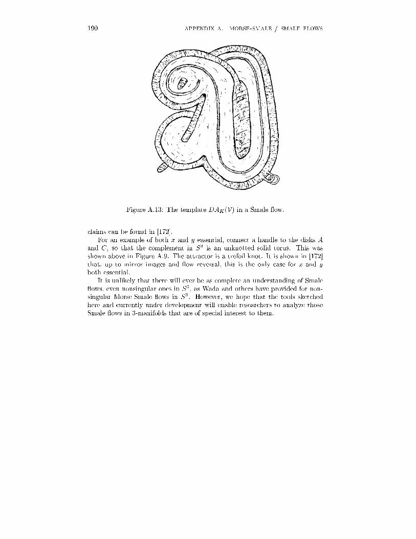
190 appendix a. morse-smale / smale flows

Figure A.13: The template DAK(V) in a Smale ow.claims can be found in [172].For an example of both x and y essential, connect a handle to the disks Aand C, so that the complement in S3 is an unknotted solid torus. This wasshown above in Figure A.9. The attractor is a trefoil knot. It is shown in [172]that, up to mirror images and ow reversal, this is the only case for x and yboth essential.It is unlikely that there will ever be as complete an understanding of Smale ows, even nonsingular ones in S3, as Wada and others have provided for non-singular Morse-Smale ows in S3. However, we hope that the tools sketchedhere and currently under development will enable researchers to analyze thoseSmale ows in 3-manifolds that are of special interest to them.

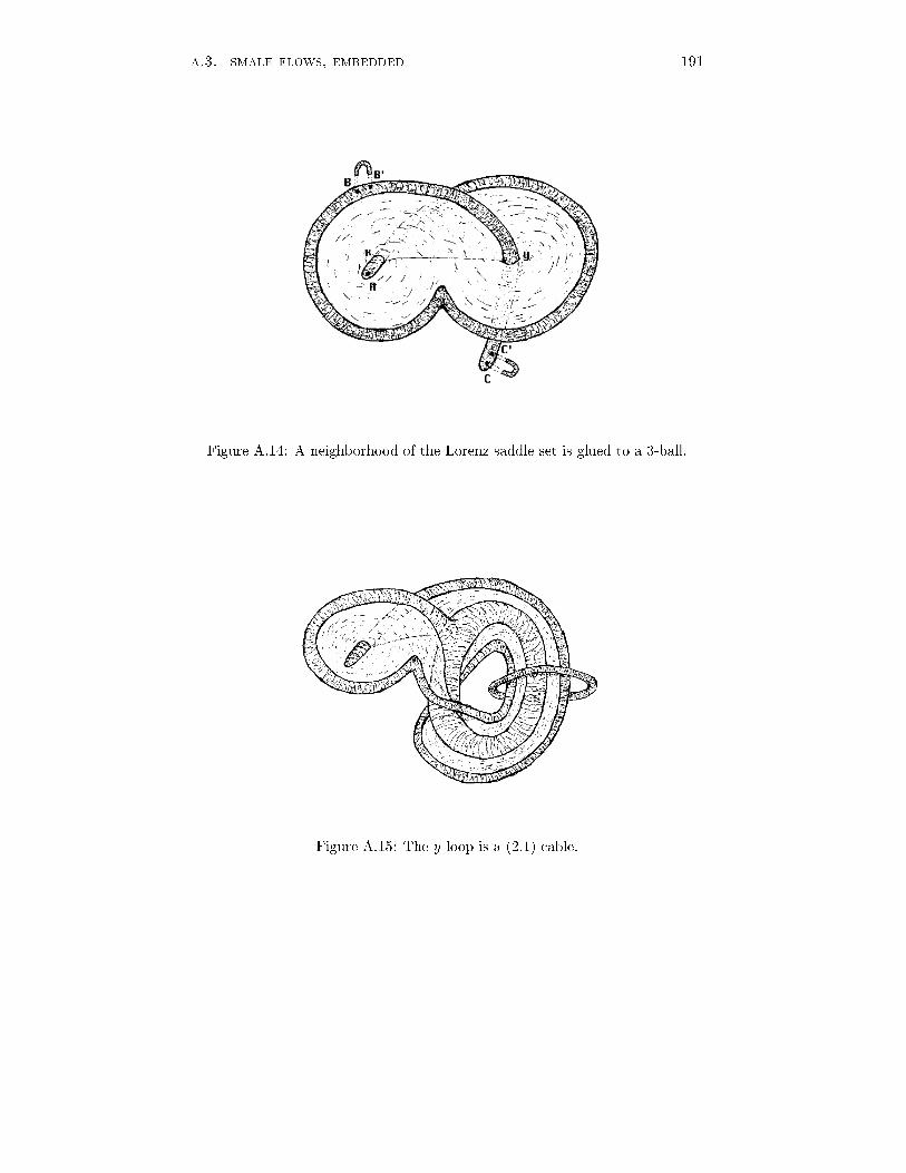
a.3. smale flows, embedded 191

Figure A.14: A neighborhood of the Lorenz saddle set is glued to a 3-ball.

Figure A.15: The y loop is a (2,1) cable.

Bibliography[1] C. Adams. The Knot Book. W. H. Freeman & Co., NY, 1994.[2] J. C. Alexander and J. Yorke. On the continuability of periodic orbitsof parametrized three dimensional di�erential equations. J. Di�. Eq.,49(2):171{184, 1983.[3] J. W. Alexander. A lemma on systems of knotted curves. Proc. Nat. Acad.Sci. USA, 9:93{95, 1923.[4] A. A. Andronov, A. A. Vitt, and S. E. Khaikin. Theory of Oscillators.Dover Publications Inc., Mineola, NY, 1987.[5] A. Arn�eodo, P. Coullet, and C. Tresser. Possible new strange attractorswith spiral structure. Commun. Math. Phys., 79:573{579, 1981.[6] V. I. Arnold. Geometrical Methods in the Theory of Ordinary Di�erentialEquations. Springer-Verlag, Berlin, Heidelberg, New York, 1982.[7] V. I. Arnold. The asymptotic Hopf invariant and its applications. Sel.Math. Sov., 5:327{345, 1986.[8] V. I. Arnold and A. Avez. Ergodic Problems of Classical Mechanics. Ben-jamin, New York, 1968.[9] D. Arrowsmith and C. Place. An Introduction to Dynamical Systems.Cambridge Press, Cambridge, 1990.[10] E. Artin. Theorie der Zopfe. Abh. Math. Sem. Univ. Hamburg, 4:47{72,1925.[11] C. Ashley. The Ashley Book of Knots. Doubleday and Co., NY, 1944.[12] D. Asimov. Round handles and non-singular Morse-Smale ows. Ann.Math., 102:41{54, 1975.[13] D. Asimov and J. Franks. Unremovable closed orbits. In J. Palis, edi-tor, Geometric Dynamics, Lecture Notes in Mathematics 1007. Springer-Verlag, 1983.[14] M. Atiyah. The Geometry and Physics of Knots. Cambridge UniversityPress, Cambridge, 1990.[15] H. Bell and K. Meyer. Limit periodic functions, adding machines, andsolenoids. Preprint, Apr. 1995. 192

BIBLIOGRAPHY 193[16] V. Belykh and L. Chua. New type of strange attractor from a geometricmodel of Chua's circuit. Int. J. Bif. Chaos, 2(3):697{704, 1992.[17] D. Bennequin. Entrelacements et �equations de Pfa�. Asterisque, 107-108:87{161, 1983.[18] G. D. Birkho�. Dynamical Systems. AMS, Providence, RI, 1927.[19] J. Birman. Braids, Links, and Mapping Class Groups. Princeton Univer-sity Press, Princeton, N.J., 1974.[20] J. Birman. Recent developments in braid and link theory. Math. Intelli-gencer, 13(1):52{60, 1991.[21] J. Birman. New points of view in knot theory. Bull. Am. Math. Soc.,28(2):253{285, 1994.[22] J. Birman and X. S. Lin. Knot polynomials and Vassiliev invariants. toappear in Invent. Math., preprint, 1995.[23] J. Birman and R. Williams. Knotted periodic orbits in dynamical systems{I : Lorenz's equations. Topology, 22(1):47{82, 1983.[24] J. Birman and R. Williams. Knotted periodic orbits in dynamical systems{II : knot holders for �bered knots. Cont. Math., 20:1{60, 1983.[25] R. Bowen. One-dimensional hyperbolic sets for ows. J. Di�. Eq., 12:173{179, 1972.[26] R. Bowen. On Axiom A di�eomorphisms. In Regional Conference Seriesin Mathematics 35, pages 1{45. National Science Foundation, AmericanMathematical Society, 1978.[27] R. Bowen and J. Franks. Homology of zero dimensional basic sets. Ann.Math., 106:73{92, 1977.[28] R. Bowen and P. Walters. Expansive one-parameter ows. J. Di�. Eq.,12:180{193, 1972.[29] P. Boyland. Braid-types of periodic orbits for surface automorphisms. InNotes on Dynamics of Surface Homeomorphisms. Warwick University, UK,Lecture notes, Maths. Inst., 1989.[30] P. Boyland. Topological methods in surface dynamics. Topology and itsApplications, 58:223{298, 1994.[31] P. Boyland and T. Hall. Dynamics of Surface Homeomorphisms. WorldScienti�c, Singapore, to appear, preprint.

194 BIBLIOGRAPHY[32] M. Boyle. Symbolic dynamics and matrices. In R.A. Bruald, S. Freedland,and V. Klee, editors, Combinatotial and graph-theoretical problems in lin-ear algebra, volume 50 of IMA Math. Appl., pages 1{38. Springer-Verlag,New York, 1993.[33] G. Burde and H. Zieschang. Knots. De Gruyter, Berlin, 1985.[34] J. Carr. Applications of Centre Manifold Theory. Springer-Verlag, Berlin,Heidelberg, New York, 1981.[35] J. Casasayas, J. Mart��nez Alfaro, and A. Nunes. Knots and links in inte-grable Hamiltonian systems. Preprint, Warwick 48/1992, Sept. 1992.[36] A. Champneys. Homoclinic tangencies in the dynamics of articulated pipesconveying uid. Physica D, 62:347{359, 1993.[37] J. Christy. Branched surfaces and attractors I: dynamic branched surfaces.Trans. Am. Math. Soc., 336(2):759{784, 1993.[38] L. Chua, M. Komuro, and T. Matsumoto. The double scroll family. IEEETrans. on Circuits and Systems, 33:1073{1118, 1986.[39] P. Collet and J. P. Eckmann. Iterated Maps on the Interval as DynamicalSystems. Birkhauser, Boston, 1980.[40] K. de Rezende. Smale ows on the three-sphere. Trans. Am. Math. Soc.,303:283{310, 1987.[41] R. Devaney. An Introduction to Chaotic Dynamical Systems. BenjaminCummings, Menlo Park, CA, 1985.[42] R. Devaney and Z. Nitecki. Shift automorphisms in the H�enon mapping.Commun. Math. Phys., 67:137{148, 1979.[43] F. Diacu and P. Holmes. Celestial Encounters: The Origins of Chaos andStability. Princeton University Press, Princeton, NJ, 1996.[44] F. Dumortier, H. Kokubu, and H. Oka. A degenerate singularity generatinggeometric Lorenz attractors. Ergod. Th. & Dynam. Sys., 15:833{856, 1995.[45] J. Etnyre and R. Ghrist. The dynamics of legendrian ows. Unpublishednotes, Oct. 1996.[46] A. Fathi, F. Laudenbach, and V. Poenaru et al. Travaux de Thurston surles surfaces. Ast�erique, 66-67:1{284, 1979.[47] M. J. Feigenbaum. Quantitative universality for a class of nonlinear trans-formations. J. Stat. Phys., 19:25{52, 1978.[48] W. Floyd and U. Oertel. Incompressible surfaces via branched surfaces.Topology, 23:117{125, 1984.

BIBLIOGRAPHY 195[49] A. T. Fomenko. Advances in Soviet Mathematics, Vol. 6. American Math-ematical Society, Providence, RI, 1991.[50] A. T. Fomenko and T. Z. Nguyen. Topological classi�cation of integrablenondegenerate Hamiltonians on isoenergy three-dimensional spheres. InA. T. Fomenko, editor, Advances in Soviet Mathematics, Vol. 6, pages267{296. American Mathematical Society, 1991.[51] J. Franks. Non-singular ows on S3 with hyperbolic chain-recurrent set.Rocky Mountain J. Math., 7(3):539{546, 1977.[52] J. Franks. Knots, links, and symbolic dynamics. Ann. of Math., 113:529{552, 1981.[53] J. Franks. Homology and Dynamical Systems, volume CBMS 49. AmericanMathematical Society, Providence, Rhode Island, 1982.[54] J. Franks. Symbolic dynamics in ows on three-manifolds. Trans. Am.Math. Soc., 279:231{236, 1983.[55] J. Franks. Flow equivalence of shifts of �nite type. Ergodic Theory andDynamical Systems, 4(1):53{66, 1984.[56] J. Franks. Nonsingular Smale ows on S3. Topology, 24:265{282, 1985.[57] J. Franks and C. Robinson. A quasi-Anosov di�eomorphism which is notAnosov. Trans. Am. Math. Soc., 223:267{278, 1976.[58] J. Franks and R. F. Williams. Entropy and knots. Trans. Am. Math. Soc.,291(1):241{253, 1985.[59] P. Freyd, D. Yetter, J. Hoste, W. B. R. Lickorish, K. Millet, and A. Oc-neanu. A new polynomial invariant of knots and links. Bull. Am. Math.Soc., 12(2):239{246, 1985.[60] G. Frobenius. �Uber Matrizen aus nicht negativen Elementen. S.B.-Deutsch. Akad. Wiss. Berlin Math.-Nat. Kl., pages 456{477, 1912.[61] D. Gabai. Foliations and the topology of 3-manifolds III. J. Di�. Geom.,26:479{536, 1987.[62] J.-M. Gambaudo and E. Ghys. Entrlacements asymptotiques. To appearin Topology, preprint, August 1996.[63] J.-M. Gambaudo, P. Glendinning, and C. Tresser. The gluing bifurcationI: symbolic dynamics of the closed curves. Nonlinearity, 1:203{214, 1988.[64] J.-M. Gambaudo, D. Sullivan, and C. Tresser. In�nite cascades of braidsand smooth dynamical systems. Topology, 33(1):85{94, 1994.

196 BIBLIOGRAPHY[65] J.-M. Gambaudo and C. Tresser. Dynamique r�eguli�ere ou chaotique: ap-plications du cercle ou de l'intervalle ayant une discontinuit�e. C. R. Acad.Sc. Paris, 300:311{313, 1985.[66] P. Gaspard, R. Kapral, and G. Nicolis. Bifurcation phenomena near ho-moclinic systems: a two-parameter family. J. Stat. Phys., 35:697{727,1984.[67] K. F. Gauss. Zur mathematischen Theorie der electrodynamischenWirkungen. Werke Konigl. Gesell. Wiss. Gottingen, 5:605, 1877.[68] R. Ghrist. Accumulations of in�nite links in ows. Preprint, August 1996.[69] R. Ghrist. Branched two-manifolds supporting all links. Topology,36(2):423{448, 1997.[70] R. Ghrist and P. Holmes. Knots and orbit genealogies in three dimensional ows. In Bifurcations and Periodic Orbits of Vector Fields, pages 185{239.NATO ASI series C volume 408, Kluwer Academic Press, 1993.[71] R. Ghrist and P. Holmes. An ODE whose solutions contain all knots andlinks. Intl. J. Bifurcation and Chaos, 6(5):779{800, 1996.[72] P. Glendinning. Global bifurcation in ows. In T. Bedford and J. Swift,editors, New Directions in Dynamical Systems, pages 120{149. LondonMath. Society, Cambridge University Press, 1988.[73] P. Glendinning, J. Los, and C. Tresser. Renormalisation between classesof maps. Phys. Lett. A, 145:109{112, 1990.[74] P. Glendinning and C. Sparrow. Local and global behavior near homoclinicorbits. J. Stat. Phys., 35:645{698, 1984.[75] P. Glendinning and C. Sparrow. T-points: a codimension two heteroclinicbifurcation. J. Stat. Phys., 43:479{488, 1986.[76] J. Guckenheimer and P. Holmes. Nonlinear Oscillations, Dynamical Sys-tems, and Bifurcations of Vector Fields. Springer-Verlag, New York, 1983.[77] J. Guckenheimer and R.Williams. Structural stability of Lorenz attractors.Inst. Hautes �Etudes Sci. Publ. Math., 50:59{72, 1979.[78] C. Gutierrez. Structural stability for ows on the torus with a cross-cap.Trans. Am. Math. Soc., 241:311{320, 1978.[79] C. Gutierrez. Knots and minimal ows on S3. Topology, 241:679{698,1995.[80] P. Hadamard. Les surfaces a cobures oppos�ees et leur lignes g�eodesiques.J. Math. Pures Appl., 4:27{73, 1898.

BIBLIOGRAPHY 197[81] V. Hansen. Braids and Coverings: Selected Topics. Cambridge UniversityPress, Cambridge, 1991.[82] A. Hatcher. On the boundary curves of incompressible surfaces. Pac. J.Math., 99(2):373{377, 1982.[83] M. H�enon. A two dimensional map with a strange attractor. Commun.Math. Phys., 50:69{77, 1976.[84] M. Hirsch, C. Pugh, and M. Shub. Invariant Manifolds, volume 583 ofSpringer Lecture Notes in Mathematics. Springer-Verlag, Berlin, Heidel-berg, New York, 1970.[85] K. Hockett and P. Holmes. Josephson's junction, annulus maps, Birkho�attractors, horseshoes and rotation sets. Ergod. Th. and Dynam. Sys.,6:205{239, 1986.[86] P. Holmes. A strange family of three-dimensional vector �elds near adegenerate singularity. J. Di�. Eq., 37(3):382{403, 1980.[87] P. Holmes. Bifurcation sequences in the horseshoe map: in�nitely manyroutes to chaos. Phys. Lett. A, 104:299{302, 1984.[88] P. Holmes. Knotted periodic orbits in suspensions of Smale's horseshoe:period mutiplying and cabled knots. Physica D, 21:7{41, 1986.[89] P. Holmes. Knotted periodic orbits in suspensions of annulus maps. Proc.Roy. London Soc. A, 411:351{378, 1987.[90] P. Holmes. Knotted periodic orbits in suspensions of Smale's horseshoe:extended families and bifurcation sequences. Physica D, 40:42{64, 1989.[91] P. Holmes and R. Ghrist. Knotting within the gluing bifurcaion. In J. M. T.Thompson and S. R. Bishop, editors, IUTAM Symposium on Nonlinearityand Chaos in Engineering Dynamics, pages 299{315. John Wiley, Chich-ester, UK, 1994.[92] P. Holmes and D. C. Whitley. On the attracting set for DuÆng's equation.Physica D, 7:111{123, 1983.[93] P. Holmes and R. F. Williams. Knotted periodic orbits in suspensionsof Smale's horseshoe: torus knots and bifurcation sequences. Archive forRational Mech. and Anal., 90(2):115 {193, 1985.[94] V. F. R. Jones. A polynomial invariant for knots via von Neumann alge-bras. Bull. Am. Math. Soc., 12(1):103{111, 1985.[95] L. Jonker and D. A. Rand. Bifurcations in one dimension I: the nonwan-dering set. Invent. Math., 62:347{365, 1981.

198 BIBLIOGRAPHY[96] L. Jonker and D. A. Rand. Bifurcations in one dimension II: a versal modelfor bifurcations. Invent. Math., 63:1{15, 1981.[97] A. Katok. Lyapunov exponents, entropy, and periodic orbits for di�eo-morphisms. Publ. Inst. Hautes �Etudes Sci., 51:137{173, 1980.[98] L. Kau�man. An invariant of regular isotopy. Trans. Am. Math. Soc.,318:417{471, 1990.[99] L. Kau�man. Knots and Physics. World Scienti�c, Singapore, 1991.[100] L. Kau�man, M. Saito, and M. Sullivan. Quantum invariants for templates.Preprint, 1996.[101] L. H. Kau�man. On Knots. Princeton University Press, Princeton, NJ,1987.[102] S. Kennedy. A Lorenz-like Strange Attractor. PhD thesis, NorthwesternUniversity, 1988.[103] S. Kennedy, M. Staford, and R. Williams. A new Caylay-Hamilton theo-rem. In Global analysis in modern mathematics, pages 247{251, Houston,TX, 1993. Publish or Perish.[104] P. Kent and J. Elgin. Noose bifurcation of periodic orbits. Nonlinearity,4:1045{1061, 1991.[105] A. Khibnik, D. Roose, and L. Chua. On periodic orbits and homoclinicbifurcations in Chua's circuit with a smooth nonlinearity. Int. J. Bif. andChaos, 3(2):363{384, 1993.[106] Lj. Kocarev, D. Dimovski, Z. Tasev, and L. Chua. Topological descriptionof a chaotic attractor with spiral structure. Phys. Lett. A, 190:399{402,1994.[107] K. Kuperberg. A smooth counterexample to the Seifert conjecture. Ann.of Math., 140:723{732, 1994.[108] C. Letellier, P. Dutertre, and G. Gouesbet. Characterization of the Lorenzsystem, taking into account the equivariance of the vector �eld. Phys. Rev.E, 49(4):3492{3495, 1994.[109] C. Letellier, P. Dutertre, and B. Maheu. Unstable periodic orbits andtemplates of the R�ossler system: toward a systematic topological charac-terization. Chaos, 5:271{282, 1995.[110] C. Letellier, P. Dutertre, J. Reizner, and G. Gouesbet. Evolution of amultimodal map induced by an equivariant vector �eld. J. Phys. A: Math.Gen., 29:5359{5373, 1996.

BIBLIOGRAPHY 199[111] C. Letellier and G. Gouesbet. Topological characterization of a systemwith high order symmetries. Phys. Rev. E, 52(5):4754{4761, 1995.[112] C. Letellier and G. Gouesbet. Topological characterization of reconstructedattractors modding out symmetries. J. Phys. II France, 6:1615{1638, 1996.[113] C. Letellier, G. Gouesbet, F. Sou�, J.R. Buchler, and Z. Koll�ath. Chaosin variable stars: topological analysis of W Vir model pulsations. Chaos,6:466{476, 1996.[114] E. Lorenz. Deterministic non-periodic ow. J. Atmospheric Sci., 20:130{141, 1963.[115] J. Los. Knots, braid index, and dynamical type. Topology, 33(2):257{270,1994.[116] L. Markus and K. Meyer. Periodic orbits and solenoids in generic Hamil-tonian systems. Amer. J. Math., 102:25{92, 1980.[117] W. Massey. Algebraic Topology, an Introduction. Springer-Verlag, Berlin,Heidelberg, New York, 1967.[118] F. McRobie and J. M. T. Thomson. Braids and knots in driven oscillators.Int. J. Bifurcation and Chaos, 3:1343{1361, 1993.[119] F. McRobie and J. M. T. Thomson. Knot types and bifurcation sequencesof homoclinic and transient orbits of a single-degree-of-freedom driven os-cillator. Submitted to Dynamics and Stability of Systems, Preprint, April1993.[120] V. K. Melnikov. On the stability of the center for time-periodic perturba-tion. Trans. Moscow Math. Soc., 12:1{57, 1963.[121] N. Merener and G. Mindlin. From time series to physical models: thecase of a pulsating star. Preprint, Departimento de F��sica, FCEN, BuenosAires, Argentina, 1996.[122] K. Meyer. Generic bifurcation of periodic points. Trans. Am. Math. Soc.,149:95{107, 1970.[123] K. Meyer. Generic stability properties of periodic points. Trans. Am.Math. Soc., 154:273{277, 1971.[124] J. Milnor. Topology from the Di�erentiable Viewpoint. University Press ofVirginia, 1969.[125] J. Milnor and W. Thurston. On iterated maps of the interval I and II.Unpublished notes, Princeton University, 1977.[126] G. Mindlin and H. Solari. Topologically inequivalent embeddings. Phys.Rev. E, 52(2):1497{1501, 1995.

200 BIBLIOGRAPHY[127] G. Mindlin and H. Solari. Tori and Klein bottles in 4 dimensional chaotic ows. Preprint, Departimento de F��sica, FCEN, Buenos Aires, Argentina,1996.[128] G. Mindlin, H. Solari, M. Natiello, R. Gilmore, and X. Hou. Topolog-ical analysis of chaotic time series data from the Belousov-Zhabotinskiireaction. J. Nonlinear Sci., 1:147{173, 1991.[129] H. Mo�at. Magnetostatic equilibria and analogous Euler ows of arbitrar-ily complex topology: part I. J. Fluid Mech., 159:359{378, 1985.[130] C. Moore. Braids in classical dynamics. Phys. Rev. Lett., 70 (24):3675{3679, 1993.[131] L. Mora and M. Viana. Abundance of strange attractors. Acta Math.,171:1{71, 1993.[132] J. Morgan. Nonsingular Morse-Smale ows on 3-dimensional manifolds.Topology, 18:41{54, 1978.[133] M. Morse. Representations of geodesics. Amer. J. Math., 43:33{51, 1921.[134] M. Morse and G. Hedlund. Symbolic dynamics. Amer. J. Math., 60:815{866, 1938.[135] J. Moser. Stable and Random Motions in Dynamical Systems. PrincetonUniversity Press, Princeton, NJ, 1973.[136] M. Muldoon, R. MacKay, J. Huke, and D. Broomhead. Topology from atime series. Physica D, 65:1{16, 1993.[137] A. Nayfeh and D. Mook. Nonlinear Oscillations. John Wiley and SonsInc., New York, 1979.[138] J. Nielsen. Untersuchungen zur Topologie der gerschlossenen zweiseitegenFl�achen I. Acta. Math., 50:189{358, 1927.[139] J. Palis and W. De Melo. Geometric theory of dynamical systems: anintroduction. Springer-Verlag, Berlin, Heidelberg, New York, 1982.[140] J. Palis and F. Takens. Hyperbolicity and Sensitive Chaotic Dynamics atHomoclinic Bifurcations. Cambridge University Press, Cambridge, NewYork, 1993.[141] B. Parry and D. Sullivan. A topological invariant of ows on 1-dimensionalspaces. Topology, 14:297{299, 1975.[142] M. Peixoto. Structural stability on two-dimensional manifolds. Topology,1:101{120, 1962.[143] O. Perron. �Uber Matrizen. Math. Ann., 64:248{263, 1907.

BIBLIOGRAPHY 201[144] R. Plykin. Sources and sinks for Axiom A di�eomorphisms. USSR Math.Sb., 23:233{253, 1974.[145] H. Poincar�e. Sur les �equations de la dynamique et le probl�eme de troiscorps. Acta Math., 13:1{270, 1890.[146] H. Poincar�e. Nouvelles Methodes de la M�ecanique C�eleste, 3 Volumes.Gauthier-Villars, Paris, 1899.[147] C. Pugh. The Closing Lemma. Amer. J. Math., 89:956{1009, 1967.[148] C. Pugh and M. Shub. Suspending subshifts. In C. Percelli and R. Sack-steder, editors, Contributions to Geometry and Analysis. London Math.Society, Johns Hopkins University Press, 1981.[149] K. Reidemeister. Knotentheorie. Springer-Verlag, Berlin, 1932.[150] J. Robbins. A structural stability theorem. Ann. Math., 94:447{493, 1971.[151] C. Robinson. Structural stability of vector �elds. Invent. Math., 99:154{175, 1974.[152] C. Robinson. Homoclinic bifurcation to a transitive attractor of Lorenztype, I. Nonlinearity, 2:495{518, 1989.[153] C. Robinson. Dynamical Systems: Stability, Symbolic Dynamics, andChaos. CRC Press, Ann Arbor, MI, 1995.[154] D. Rolfsen. Knots and Links. Publish or Perish, Berkely, CA, 1977.[155] A. Rucklidge. Chaos in a low-order model of magnetoconvection. PhysicaD, 62:323{337, 1993.[156] M. Rychlik. Lorenz attractors through Silnikov-type bifurcation: part I.Ergod. Th. & Dynam. Sys., 10:793{821, 1989.[157] M. Saito. On closed orbits of Morse-Smale ows on 3-manifolds. Bull.Lond. Math. Soc., 23:482{486, 1990.[158] S. Sawin. Links, quantum groups and TQFTs. Bull. of the A.M.S.,33(4):413{445, 1996.[159] L. Le Sceller, C. Letellier, and G. Gouesbet. Algebraic evaluation of linkingnumbers of unstable periodic orbits in chaotic attractors. Phys. Rev. E,49(5):4693{4695, 1994.[160] L. P. Shil'nikov. A case of the existence of a countable number of periodicmotions. Soviet Math. Dokl., 6:163{166, 1965.[161] L. P. Shil'nikov. A contribution to the problem of the structure of anextended neighborhood of a rough equilibrium state of saddle-focus type.Math. USSR Sbornik, 10(1):91{102, 1970.

202 BIBLIOGRAPHY[162] M. Shub. Global Stability of Dynamical Systems. Springer-Verlag, Berlin,Heidelberg, New York, 1987.[163] D. Singer. Stable orbits and bifurcations of maps of the interval. SIAM J.Appl. Math., 35:260{267, 1978.[164] S. Smale. Stable manifolds for di�erential equations and di�eomorphisms.Ann. Scuola Normale Pisa, 18:97{116, 1963.[165] S. Smale. Di�erentiable dynamical systems. Bull. Am. Math. Soc., 73:747{817, 1967.[166] C. Sparrow. The Lorenz Equations: Bifurcations, Chaos and Strange At-tractors, volume 41 of Applied Mathematical Sciences. Springer-Verlag,New York, NY, 1982.[167] J. Stallings. On �bering certain 3-manifolds. In M. K. Fort Jr., editor,Topology of 3-Manifolds, pages 95{100. Prentice-Hall, 1962.[168] M. Sullivan. Prime decomposition of knots in Lorenz-like templates. J.Knot Thy. and Ram., 2(4):453{462, 1993.[169] M. Sullivan. The prime decomposition of knotted periodic orbits in dy-namical systems. J. Knot Thy. and Ram., 3(1):83{120, 1994.[170] M. Sullivan. An invariant for basic sets of Smale ows. Preprint, 1995.[171] M. Sullivan. A zeta function for positive templates. Top. and its Appl.,66(3):199{213, 1995.[172] M. Sullivan. Visualizing Smale ows in S3. Work in progress, 1996.[173] D. Sumners. Untangling DNA. Math. Intelligencer, 12:71{80, 1990.[174] P. Tait. On knots I, II, III. Technical report, Cambridge Univ. Press,London., 1898.[175] F. Takens. Detecting strange attractors in turbulence. volume 898 ofSpringer Lecture Notes in Mathematics, pages 365{381, Berlin, Heidelberg,New York, 1980. Springer-Verlag.[176] W. Thomson. On vortex motion. Trans. R. Soc. Edin., 25:217{260, 1869.[177] W. Thurston. The geometry and topology of three-manifolds. Unpublishednotes, Princeton Math. Dept., 1979.[178] W. Thurston. On the geometry and dynamics of di�eomorphisms of sur-faces. Bull. Am. Math. Soc., 19(2):417{431, 1988.[179] C. Tresser. About some theorems by L. P. Shil'nikov. Ann. Inst. H.Poincar�e, 40:441{461, 1984.

BIBLIOGRAPHY 203[180] N. Tu�llaro. Topological organization of (low dimensional) chaos. In J. P.Nadal and P. Grassberger, editors, From Statistical Physics to StatisticalInference and Back. NATO ASI series C, Kluwer Academic Press, 1994.[181] S. Ulam and J. von Neumann. On combinations of stochastic and deter-ministic processes. Bull. Am. Math. Soc., 53:11{20, 1947.[182] J. VanBuskirk. Positive knots have positive Conway polynomials. InD. Rolfsen, editor, Knot Theory and Manifolds, volume 1144 of LectureNotes in Mathematics, pages 146{159. Springer-Verlag, 1985.[183] V. Vassiliev. Cohomology of knot spaces. In V. I. Arnold, editor, Theoryof Singularities and its Applications, pages 23{69, Providence, RI, 1990.Amer. Math. Soc.[184] M. Wada. Closed orbits of nonsingular Morse-Smale ows on S3. J. Math.Soc. Japan, 41(3):405{413, 1989.[185] J. Wagoner. Markov partitions and K2. Inst. Hautes �Etudes Sci. Publ.Math., 65:91{129, 1987.[186] J. Wagoner. Topological Markov chains, C�-algbras and K2. Advances inMathematics, 71(2):133{185, 1988.[187] F. Wicklin. Dynamics near resonance in multi-frequency systems. PhDthesis, Cornell University, 1993.[188] S. Wiggins. Global Bifurcations and Chaos: Analytical Methods. Springer-Verlag, Berlin, Heidelberg, New York, 1988.[189] S. Wiggins. Introduction to Applied Nonlinear Dynamical Systems andChaos. Springer-Verlag, Berlin, Heidelberg, New York, 1990.[190] R. Williams. The DA maps of Smale and structural stability. In GlobalAnalysis, volume XIV, pages 329{334, Providence, RI, 1970. AMS.[191] R. Williams. Classi�cation of subshifts of �nite type. Ann. of Math.,98:120{153, 1973.[192] R. Williams. Expanding attractors. Inst. Hautes �Etudes Sci. Publ. Math.,43:169{203, 1974.[193] R. Williams. The structure of Lorenz attractors. In A. Chorin, J. Marsden,and S. Smale, editors, Turbulence Seminar, Berkeley 1976/77, volume 615of Springer Lecture Notes in Mathematics, pages 94{116, 1977.[194] R. Williams. The structure of Lorenz attractors. Inst. Hautes �Etudes Sci.Publ. Math., 50:73{79, 1979.[195] R. Williams. Lorenz knots are prime. Ergod. Th. and Dynam. Sys., 4:147{163, 1983.

204 BIBLIOGRAPHY[196] R. Williams. A new zeta funtion, natural for links. In From Topologyto Computation; Proceedings of the Smalefest, pages 270{278, New York,NY, 1993. Springer-Verlag.[197] E. Witten. Quantum �eld theory and the Jones polynomial. Comm. Math.Phys., 121:355{399, 1989.[198] J. Yorke and K. Alligood. Cascades of period-doubling bifurcations: aprerequisite for horseshoes. Bull. Am. Math. Soc., 9:319{322, 1983.[199] J. Yorke and K. Alligood. Period-doubling cascades of attractors: a pre-requisite for horseshoes. Commun. Math. Phys., 101:305{321, 1985.

Index�-factorizable, 123�-prime, 123accumulations, 75, 77, 105adjacent, 70admissible, 22Alexander polynomial, 184Alexander's Theorem, 12, 69Anosov, 17appending an ear, 85attaching zone, 173attractor, 35expanding, 35hyperbolic, 35, 43Lorenz, 33Plykin, 36, 91belt trick, 64Bennequin inequality, 16, 73bifurcationgluing, 129H�enon map, 119homoclinic, 129Hopf, 29, 108noose, 111pair, 114period-doubling, 28, 108period-multiplying, 109pitchfork, 28, 108saddle-node, 28, 108, 121boundary, 62, 144braid, 10axis, 12closed, 11generators, 11group, 10, 83template, 98positive, 12template, 69braid index, 16, 117branch line, 38branch segment, 61

branched manifold, 34cable, 9chain recurrent set ow, 21map, 19companion, 9composite, 8computed twist, 155concatenation, 70conjugacy, 17conjugatein ation, 81connected sum, 8DA, 42DuÆng equation, 49edge graph, 23elliptic orbit, 109entropy, 26equilibrium, 17equivalenceexpansion, 147 ow, 147strong shift, 146template, 143essential, 176expanding attractor, 35expansion equivalence, 147faithful, 9Farey mediant, 133Farey neighbors, 130female orbit, 114, 124�bred, 54�gure eight template, 56�gure-eight knot, 5, 95�xed point, 17 ow, 20hyperbolic, 21Morse-Smale, 22, 171205

206 INDEXSmale, 22, 181stable manifold, 21Stable Manifold Theorem, 22suspension, 20unstable manifold, 21 ow equivalence, 147, 150generalized iterated torus knot, 10genus, 13Bennequin inequality, 16, 73concatenation, 72torus knot, 14gluing bifurcation, 129butter y, 130�gure-of-eight, 130H�enon map, 119Hamiltonian systems, 180homoclinic, 26Hopf bifurcation, 29, 108Hopf link, 12, 171horseshoemap, 25template, 48, 112torus knots, 115hyperbolicattractor, 35, 43 ow, 21map, 17orbit, 109induced template, 105inessential, 176in ation, 66conjugate, 81isotopic, 67symbolic action, 67invariant, 13braid index, 16, 117genus, 13knot, 145linking number, 13Parry-Sullivan, 147, 150self-linking number, 110template, 143twist, 156

invariant coordiante, 30inverse limit, 35irreducible, 146irreducible template, 75isotopicambient, 6braid, 10in ation, 67knot, 6renormalization, 65torus knot, 8iteratedhorseshoe knot, 124torus knot, 9, 127itinerary, 22, 31period, 63rotation compatible, 130joining chart, 38kneadingfactorization, 122invariant, 32, 122knot, 5cable, 9companion, 9composite, 8�bred, 54�gure-eight, 5, 95invariant, 13iteratedhorseshoe, 124oriented, 5presentation, 7prime, 8satellite, 9torus, 7generalized iterated, 10horseshoe, 115iterated, 9, 127resonant, 112trefoil, 5unknot, 5link, 5Hopf, 12, 171

INDEX 207planetary, 55separable, 13Whitehead, 13, 56linking matrix, 184linking number, 13local stable/unstable manifold ow, 21local stable/unstable manifoldsmap, 19Lorenz attractor, 33Lorenz template, 47Lorenz-like template, 47, 78, 90, 93Lyapunov graph, 181, 185M�obius orbit, 109male orbit, 114, 124mapH�enon, 119hyperbolic, 17monodromy, 54Morse-Smale di�eomorphism, 20Poincar�e, 20pseudo-Anosov, 56Smale di�eomorphism, 20Smale horseshoe, 25Stable Manifold Theorem, 19toral Anosov, 18Markov partition, 24minimal, 31modi�ed twist, 155monodromy, 54Morse-Smaledi�eomorphism, 20 ow, 22, 171Nielsen-Thurston Theorem, 55no-cycle property, 174noose bifurcation, 111orbit, 16elliptic, 109female, 114, 124genealogies, 129hyperbolic, 109M�obius, 109male, 114, 124

parity matrix, 149Parry-Sullivan invariant, 147, 150pattern, 9period-doubling bifurcation, 28, 108periodic, 56pitchfork bifurcation, 28, 108planetary link, 55Plykin attractor, 36, 91Poincar�e map, 20Poincar�e-Birkho�-SmaleHomoclinicTheorem, 26positivetemplate, 69positive template, 76, 154presentation, 7prime, 8pseudo-Anosov, 56rectangle, 24rectangles, 39reducible, 56Reidemeister moves, 7, 13renormalization, 64isotopic, 65resonant torus knot, 112RH decomposition, 174ribbon set, 150rotation compatible, 130round handle, 173saddle-node bifurcation, 28, 108in H�enon map, 121satellite, 9Seifert Conjecture, 75Seifert surface, 14, 54self-linking number, 110semiconjugate, 23shift map �, 22Shil'nikov connection, 51, 134Smaledi�eomorphism, 20 ow, 22, 181split sum, 175splitting chart, 38stable manifold ow, 21

208 INDEXlocal, 21map, 19local, 19Stable Manifold Theorem, 19 ow, 22strong shift equivalence, 146structural stability, 17structure matrix, 182subshift of �nite type, 22, 105, 145one-sided, 24subtemplate, 64, 97suspension, 20syllables, 117symbolic dynamics, 22symbolic period, 63template, 37boundary, 62branch line, 38branch segment, 61companion, 124equivalence, 143�gure eight, 56gluingbutter y, 130�gure-of-eight, 130horseshoe, 48, 112induced, 57, 105in ation, 66isotopic, 67irreducible, 75joining chart, 38Lorenz, 47Lorenz-like, 47, 78, 90, 93moves, 143normal form, 38positive, 69, 76, 154renormalization, 64isotopic, 65ribbon set, 150satellite, 124Shil'nikovdouble, 137single, 135splitting chart, 38subtemplate, 64, 97

Template Theorem, 38universal, 69, 78, 89V , 65, 79Whitehead, 56zeta function, 157Template Theorem, 38time series, 57topological entropy, 26toral Anosov map, 18torus knot, 7generalized iterated, 10genus, 14horseshoe, 115iterated, 9, 127resonant, 112transition matrix, 22trefoil, 5twistcomputed, 155matrix, 157modi�ed, 155usual, 155universal template, 69, 78, 89unknot, 5, 55unlinked, 13unstable manifold ow, 21local, 21map, 19local, 19usual twist, 155V , 65, 79vertex graph, 23Wada Theorem, 179Whitehead link, 13, 56Zeeman number, 185zeta function, 154, 157