Kirkwood gaps and diffusion along mean motion …fejoz/Articles/Fejoz-Guardia... · The proof...
89
DOI 10.4171/JEMS/642 J. Eur. Math. Soc. 18, 2313–2401 c European Mathematical Society 2016 Jacques F´ ejoz · Marcel Gu` ardia · Vadim Kaloshin · Pablo Rold´ an Kirkwood gaps and diffusion along mean motion resonances in the restricted planar three-body problem Received January 27, 2014 Abstract. We study the dynamics of the restricted planar three-body problem near mean motion resonances, i.e. a resonance involving the Keplerian periods of the two lighter bodies revolving around the most massive one. This problem is often used to model Sun-Jupiter-asteroid systems. For the primaries (Sun and Jupiter), we pick a realistic mass ratio μ = 10 -3 and a small eccentricity e 0 > 0. The main result is a construction of a variety of non-local diffusing orbits which show a drastic change of the osculating (instant) eccentricity of the asteroid, while the osculating semi- major axis is kept almost constant. The proof relies on the careful analysis of the circular problem, which has a hyperbolic structure, but for which diffusion is prevented by KAM tori. In the proof we verify certain non-degeneracy conditions numerically. Based on the work of Treschev, it is natural to conjecture that the time of diffusion for this problem is ∼- ln(μe 0 )/(μ 3/2 e 0 ). We expect our instability mechanism to apply to realistic values of e 0 and we give heuristic arguments in its favor. If so, the applicability of Nekhoroshev theory to the three-body problem as well as the long time stability become questionable. It is well known that, in the Asteroid Belt, located between the orbits of Mars and Jupiter, the distribution of asteroids has the so-called Kirkwood gaps exactly at mean motion resonances of low order. Our mechanism gives a possible explanation of their existence. To relate the existence of Kirkwood gaps to Arnol’d diffusion, we also state a conjecture on its existence for a typical ε-perturbation of the product of the pendulum and the rotator. Namely, we predict that a positive conditional measure of initial conditions concentrated in the main resonance exhibits Arnol’d dif- fusion on time scales -(ln ε)/ε 2 . Keywords. Three-body problem, instability, resonance, hyperbolicity, Mather mechanism, Arnol’d diffusion, Solar System, Asteroid Belt, Kirkwood gap J. F´ ejoz: Universit´ e Paris-Dauphine, CEREMADE, Place du Mar´ echal de Lattre, 75016 Paris, and Observatoire de Paris, IMCCE, 77 avenue Denfert-Rochereau, 75014 Paris, France; e-mail: [email protected] M. Gu` ardia: Institut de Math´ ematiques de Jussieu, Universit´ e Paris 7 Denis Diderot, F-75205 Paris Cedex 13, France: e-mail: [email protected], [email protected] V. Kaloshin: Department of Mathematics, University of Maryland, Mathematics Building, College Park, MD 20742-4015, USA; e-mail: [email protected] P. Rold´ an: Departament de Matem` atica Aplicada I Escola T` ecnica Superior d’Enginyeria Industrial de Barcelona, Av. Diagonal 647, 08028 Barcelona, Spain; e-mail: [email protected] Mathematics Subject Classification (2010): 70F15, 37J40
Transcript of Kirkwood gaps and diffusion along mean motion …fejoz/Articles/Fejoz-Guardia... · The proof...

DOI 10.4171/JEMS/642
J. Eur. Math. Soc. 18, 2313–2401 c© European Mathematical Society 2016
Jacques Fejoz ·Marcel Guardia · Vadim Kaloshin · Pablo Roldan
Kirkwood gaps and diffusion along mean motionresonances in the restricted planar three-body problem
Received January 27, 2014
Abstract. We study the dynamics of the restricted planar three-body problem near mean motionresonances, i.e. a resonance involving the Keplerian periods of the two lighter bodies revolvingaround the most massive one. This problem is often used to model Sun-Jupiter-asteroid systems.For the primaries (Sun and Jupiter), we pick a realistic mass ratioµ = 10−3 and a small eccentricitye0 > 0. The main result is a construction of a variety of non-local diffusing orbits which show adrastic change of the osculating (instant) eccentricity of the asteroid, while the osculating semi-major axis is kept almost constant. The proof relies on the careful analysis of the circular problem,which has a hyperbolic structure, but for which diffusion is prevented by KAM tori. In the proof weverify certain non-degeneracy conditions numerically.
Based on the work of Treschev, it is natural to conjecture that the time of diffusion for thisproblem is∼ − ln(µe0)/(µ
3/2e0). We expect our instability mechanism to apply to realistic valuesof e0 and we give heuristic arguments in its favor. If so, the applicability of Nekhoroshev theory tothe three-body problem as well as the long time stability become questionable.
It is well known that, in the Asteroid Belt, located between the orbits of Mars and Jupiter, thedistribution of asteroids has the so-called Kirkwood gaps exactly at mean motion resonances oflow order. Our mechanism gives a possible explanation of their existence. To relate the existenceof Kirkwood gaps to Arnol’d diffusion, we also state a conjecture on its existence for a typicalε-perturbation of the product of the pendulum and the rotator. Namely, we predict that a positiveconditional measure of initial conditions concentrated in the main resonance exhibits Arnol’d dif-fusion on time scales −(ln ε)/ε2.
Keywords. Three-body problem, instability, resonance, hyperbolicity, Mather mechanism, Arnol’ddiffusion, Solar System, Asteroid Belt, Kirkwood gap
J. Fejoz: Universite Paris-Dauphine, CEREMADE, Place du Marechal de Lattre, 75016 Paris, andObservatoire de Paris, IMCCE, 77 avenue Denfert-Rochereau, 75014 Paris, France;e-mail: [email protected]. Guardia: Institut de Mathematiques de Jussieu, Universite Paris 7 Denis Diderot,F-75205 Paris Cedex 13, France: e-mail: [email protected], [email protected]. Kaloshin: Department of Mathematics, University of Maryland, Mathematics Building, CollegePark, MD 20742-4015, USA; e-mail: [email protected]. Roldan: Departament de Matematica Aplicada I Escola Tecnica Superior d’Enginyeria Industrialde Barcelona, Av. Diagonal 647, 08028 Barcelona, Spain; e-mail: [email protected]
Mathematics Subject Classification (2010): 70F15, 37J40

2314 Jacques Fejoz et al.
Contents
1. Introduction and main results . . . . . . . . . . . . . . . . . . . . . . . . . . . . . . . 23151.1. The problem of the stability of gravitating bodies . . . . . . . . . . . . . . . . . 23151.2. An example of relevance in astronomy . . . . . . . . . . . . . . . . . . . . . . . 23171.3. Main results . . . . . . . . . . . . . . . . . . . . . . . . . . . . . . . . . . . . . 23191.4. Refinements and comments . . . . . . . . . . . . . . . . . . . . . . . . . . . . . 23221.5. Mechanism of instability . . . . . . . . . . . . . . . . . . . . . . . . . . . . . . 23241.6. Sketch of the proof . . . . . . . . . . . . . . . . . . . . . . . . . . . . . . . . . 23251.7. Nature of numerics . . . . . . . . . . . . . . . . . . . . . . . . . . . . . . . . . 23271.8. Main theorem for the 1 : 7 resonance . . . . . . . . . . . . . . . . . . . . . . . . 2328
2. The circular problem . . . . . . . . . . . . . . . . . . . . . . . . . . . . . . . . . . . 23302.1. Normally hyperbolic invariant cylinders . . . . . . . . . . . . . . . . . . . . . . 23302.2. The inner map . . . . . . . . . . . . . . . . . . . . . . . . . . . . . . . . . . . . 23342.3. The outer map . . . . . . . . . . . . . . . . . . . . . . . . . . . . . . . . . . . . 2334
3. The elliptic problem . . . . . . . . . . . . . . . . . . . . . . . . . . . . . . . . . . . . 23393.1. The specific form of the inner and outer maps . . . . . . . . . . . . . . . . . . . 23393.2. The e0-expansion of the elliptic Hamiltonian . . . . . . . . . . . . . . . . . . . . 23423.3. Perturbative analysis of the flow . . . . . . . . . . . . . . . . . . . . . . . . . . 23433.4. Perturbative analysis of the invariant cylinder and its inner map . . . . . . . . . . 23453.5. The outer map . . . . . . . . . . . . . . . . . . . . . . . . . . . . . . . . . . . . 2348
4. Existence of diffusing orbits . . . . . . . . . . . . . . . . . . . . . . . . . . . . . . . 23504.1. Existence of a transition chain of whiskered tori . . . . . . . . . . . . . . . . . . 23504.2. Shadowing . . . . . . . . . . . . . . . . . . . . . . . . . . . . . . . . . . . . . 2354
Appendix A. Numerical study of the normally hyperbolic invariant cylinder of the circularproblem . . . . . . . . . . . . . . . . . . . . . . . . . . . . . . . . . . . . . . . . . . 2355A.1. Computation of the periodic orbits . . . . . . . . . . . . . . . . . . . . . . . . . 2356A.2. Computation of invariant manifolds . . . . . . . . . . . . . . . . . . . . . . . . 2361A.3. Computation of transversal homoclinic points and splitting angle . . . . . . . . . 2364A.4. Accuracy of computations . . . . . . . . . . . . . . . . . . . . . . . . . . . . . 2368
Appendix B. Numerical study of the inner and outer dynamics . . . . . . . . . . . . . . . 2369B.1. From Cartesian to Delaunay and computation of ∂G1Hcirc . . . . . . . . . . . . 2371B.2. Inner and outer dynamics of the circular problem . . . . . . . . . . . . . . . . . 2372B.3. Inner and outer dynamics of the elliptic problem . . . . . . . . . . . . . . . . . . 2375B.4. Comparison of the inner and outer dynamics of the elliptic problem . . . . . . . 2378
Appendix C. The Main Result for the 3 : 1 resonance: instabilities in the Kirkwood gaps . . 2378C.1. The circular problem . . . . . . . . . . . . . . . . . . . . . . . . . . . . . . . . 2379C.2. The elliptic problem . . . . . . . . . . . . . . . . . . . . . . . . . . . . . . . . . 2383C.3. Numerical study of the 3 : 1 resonance . . . . . . . . . . . . . . . . . . . . . . . 2386
Appendix D. Conjectures on the speed of diffusion . . . . . . . . . . . . . . . . . . . . . 2391D.1. Speed of diffusion for a priori unstable systems and positive measure . . . . . . . 2393D.2. Structure of the restricted planar elliptic three-body problem . . . . . . . . . . . 2394D.3. The Mather accelerating problem and its speed of diffusion . . . . . . . . . . . . 2395D.4. Modified positive measure conjecture . . . . . . . . . . . . . . . . . . . . . . . 2396
References . . . . . . . . . . . . . . . . . . . . . . . . . . . . . . . . . . . . . . . . . . . 2397

Restricted planar three-body problem 2315
1. Introduction and main results
1.1. The problem of the stability of gravitating bodies
The stability of the Solar System is a longstanding problem. Over the centuries, mathe-maticians and astronomers have spent an inordinate amount of energy proving strongerand stronger stability theorems for dynamical systems closely related to the Solar System,generally within the framework of the Newtonian N -body problem:
qi =∑j 6=i
mjqj − qi
‖qj − qi‖3, qi ∈ R2, i = 0, 1, . . . , N − 1, (1)
and its planetary subproblem, where the massm0 (modelling the Sun) is much larger thanthe other masses mi [FejS13].
A famous theorem of Lagrange entails that the observed variations in the motion ofJupiter and Saturn come from resonant terms of large amplitude and long period, but withzero average (see [Las06] and references therein, or [AKN88, Example 6.16]). Yet it is amistake, which Laplace made, to infer the topological stability of the planetary system,since the theorem deals only with an approximation of the first order with respect to themasses, eccentricities and inclinations of the planets, outside mean motion resonances[Lap89, p. 296]. Another key result is Arnol’d’s theorem, which proves the existence ofa set of positive Lebesgue measure filled by invariant tori in planetary systems, providedthat the masses of the planets are small [Arn63, Fej04]. However, in the phase space thegaps left by the invariant tori leave room for instability.
It was a big surprise when the numerical computations of Sussman, Wisdom andLaskar showed that over the life span of the Sun, or even over a few million years, col-lisions and ejections of inner planets are probable (due to the exponential divergence ofsolutions, only a probabilistic result seems within the reach of numerical experiments);see for example [SW92, Las94], or [Las10] for a recent account. Our Solar System, aswell as newly discovered extra-solar systems, are now widely believed to be unstable,and the general conjecture about theN -body problem is quite the opposite of what it usedto be:
Conjecture 1.1 (Global instability of the N -body problem). On restriction to any en-ergy level of the N -body problem, the non-wandering set is nowhere dense. (One canreparameterize orbits to have a complete flow, despite collisions.)
According to Herman [Her98], this is the oldest open problem in dynamical systems (seealso [Kol57]). This conjecture would imply that bounded orbits form a nowhere denseset and that no topological stability whatsoever holds, in a very strong sense. It is largelyconfirmed by numerical experiments. In our Solar System, Laskar for instance has shownthat collisions between Mars and Venus could occur within a few billion years. The co-existence of a nowhere dense set of positive measure of bounded quasi-periodic motionswith an open and dense set of initial conditions with unbounded orbits is a remarkableconjecture.
Currently the above conjecture is largely out of reach. A more modest but still verychallenging goal, also stated in [Her98], is a local version of the conjecture:

2316 Jacques Fejoz et al.
Conjecture 1.2 (Instability of the planetary problem). If the masses of the planets aresmall enough, the wandering set accumulates on the set of circular, coplanar, Keplerianmotions.
There have been some prior attempts to prove such a conjecture. For instance, Moeckeldiscovered an instability mechanism in a special configuration of the 5-body prob-lem [Moe96]. His proof of diffusion was limited by the so-called big gaps problembetween hyperbolic invariant tori; this problem was later solved in this setting byZheng [Zhe10]. A somewhat opposite strategy was developed by Bolotin and McKay, us-ing the Poincare orbits of the second species to show the existence of symbolic dynamicsin the three-body problem, hence of chaotic orbits, but considering far from integrable,non-planetary conditions; see for example [Bol06]. Also, Delshams, Gidea and Roldanhave shown an instability mechanism in the spatial restricted three-body problem, butonly locally around the equilibrium point L1 (see [DGR11]).
In this paper we prove the existence of large instabilities in a realistic planetary systemand describe the associated instability mechanism. We thus provide a step towards theproof of Conjecture 1.2.
In his famous paper [Arn64], Arnol’d says: “In contradistinction with stability, insta-bility1 is itself stable. I believe that the mechanism of “transition chain” which guaranteesthat instability in our example is also applicable to the general case (for example, to theproblem of three bodies)”. In this paper we exhibit a regime of realistic motions of athree-body problem where “transition chains” do occur and lead to Arnol’d’s mechanismof instability. Such instabilities occur near mean motion resonances, defined below. To thebest of our knowledge, this is the first regime of motions of the problem of three bodiesnaturally modelling a region in the Solar System where non-local transition chains areestablished.2 Our instability results complement the KAM stability results in the heuristicpicture of asteroid dynamics described by J. Moser [Mos79]. Previous results showingtransition chains of tori in the problem of three bodies naturally modelling a region in theSolar System are confined to small neighborhoods of the Lagrangian equilibrium points[CZ11, DGR11], and therefore are local in the configuration and phase space.
The instability mechanism shown in this paper is related to a generalized versionof Mather’s acceleration problem [Mat96, BT99, DdlLS00, GT08, Kal03, Pif06]. Someparts of the proof rely on numerical computations, but our strategy allows us to keep thesecomputations simple and convincing.
We consider the planetary problem (1) with one planet mass (say, m1) larger thanthe others: m0 � m1 � m2, . . . , mN−1. The equations of motion of the lighter objects(i = 2, . . . , N − 1) can advantageously be written as
qi = m0q0 − qi
‖q0 − qi‖3+m1
q1 − qi
‖q1 − qi‖3+
∑j 6=i, j>1
mjqj − qi
‖qj − qi‖3. (2)
1 In the translation the word “nonstability” is used, which seems to refer to instability.2 “Non-local” means that motions on the boundary tori in this chain differ significantly, uniformly
with respect to the small parameter. In our case, the eccentricity of orbits of the massless planet(asteroid) varies by O(1), uniformly with respect to small values of the eccentricity of the primaries,while the semi-major axis stays nearly constant. See Section 1.3 for more details.

Restricted planar three-body problem 2317
Letting the masses mj tend to 0 for j = 2, . . . , N − 1, we obtain a collection of N − 2independent restricted problems:
qi = m0q0 − qi
‖q0 − qi‖3+m1
q1 − qi
‖q1 − qi‖3, (3)
where the massless bodies are influenced by, without themselves influencing, the pri-maries of masses m0 and m1.
For N = 3, this model is often used to approximate the dynamics of Sun-Jupiter-asteroid or other Sun-planet-object problems, and it is the simplest one conjectured tohave a wide range of instabilities.
1.2. An example of relevance in astronomy
1.2.1. The Asteroid Belt. One place in the Solar System where the dynamics is wellapproximated by the restricted three-body problem is the Asteroid Belt. The AsteroidBelt is located between the orbits of Mars and Jupiter and consists of 1.7 million objectsranging from asteroids of 950 kilometers across to dust particles. Since the mass of Jupiteris approximately 2960 masses of Mars, away from close encounters with Mars, one canneglect the influence of Mars on the asteroids and focus on the influence of Jupiter. Wealso omit interactions with the second biggest planet in the Solar System, namely Saturn,which actually is not so small. Indeed, its mass is about a third of the mass of Jupiter andits semi-major axis is about 1.83 times the semi-major axis of Jupiter. This implies thatthe strength of interaction with Saturn is around 10% of the strength of interaction withJupiter. However, instabilities discussed in this paper are fairly robust and we believe thatthey are not destroyed by the interaction with Saturn (or other celestial bodies), which tosome degree averages out.
With these assumptions one can model the motion of the objects in the Asteroid Beltby the restricted problem. Denote by µ = m1/(m0 +m1) the mass ratio, where m0 is themass of the Sun andm1 is the mass of Jupiter. For µ = 0 (that is, neglecting the influenceof Jupiter), bounded orbits of the asteroid are ellipses. Up to orientation, the ellipses arecharacterized by their semi-major axis a and eccentricity e.
The aforementioned theorem of Lagrange asserts that, for small µ > 0, the semi-major axis a(t) of an asteroid satisfies |a(t)− a(0)| . µ for all |t | . 1/µ. For very smallµ the time of stability was greatly improved by Niederman [Nie96] using Nekhoroshevtheory; see the discussion in the next section. Nevertheless, if one looks at the asteroiddistribution in terms of their semi-major axis, one encounters several gaps, the so-calledKirkwood gaps. It is believed that the existence of these gaps is due to instability mecha-nisms.
1.2.2. Kirkwood gaps and Wisdom’s ejection mechanism. Mean motion resonances oc-cur when the ratio between the period of Jupiter and the period of the asteroid is rational.In particular, the Kirkwood gaps correspond to the ratios 3 : 1, 5 : 2 and 7 : 3.
In this section we present a heuristic explanation of the reason why these gaps exist.
2318 Jacques Fejoz et al.
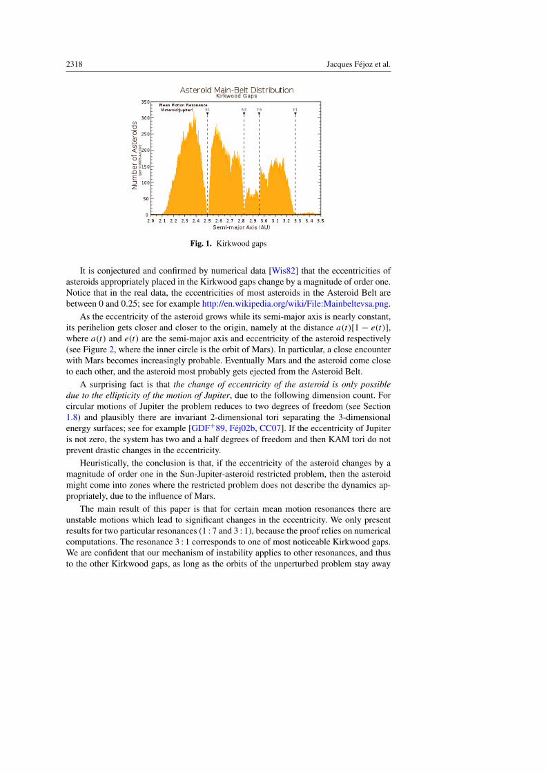
Fig. 1. Kirkwood gaps
It is conjectured and confirmed by numerical data [Wis82] that the eccentricities ofasteroids appropriately placed in the Kirkwood gaps change by a magnitude of order one.Notice that in the real data, the eccentricities of most asteroids in the Asteroid Belt arebetween 0 and 0.25; see for example http://en.wikipedia.org/wiki/File:Mainbeltevsa.png.
As the eccentricity of the asteroid grows while its semi-major axis is nearly constant,its perihelion gets closer and closer to the origin, namely at the distance a(t)[1 − e(t)],where a(t) and e(t) are the semi-major axis and eccentricity of the asteroid respectively(see Figure 2, where the inner circle is the orbit of Mars). In particular, a close encounterwith Mars becomes increasingly probable. Eventually Mars and the asteroid come closeto each other, and the asteroid most probably gets ejected from the Asteroid Belt.
A surprising fact is that the change of eccentricity of the asteroid is only possibledue to the ellipticity of the motion of Jupiter, due to the following dimension count. Forcircular motions of Jupiter the problem reduces to two degrees of freedom (see Section1.8) and plausibly there are invariant 2-dimensional tori separating the 3-dimensionalenergy surfaces; see for example [GDF+89, Fej02b, CC07]. If the eccentricity of Jupiteris not zero, the system has two and a half degrees of freedom and then KAM tori do notprevent drastic changes in the eccentricity.
Heuristically, the conclusion is that, if the eccentricity of the asteroid changes by amagnitude of order one in the Sun-Jupiter-asteroid restricted problem, then the asteroidmight come into zones where the restricted problem does not describe the dynamics ap-propriately, due to the influence of Mars.
The main result of this paper is that for certain mean motion resonances there areunstable motions which lead to significant changes in the eccentricity. We only presentresults for two particular resonances (1 : 7 and 3 : 1), because the proof relies on numericalcomputations. The resonance 3 : 1 corresponds to one of most noticeable Kirkwood gaps.We are confident that our mechanism of instability applies to other resonances, and thusto the other Kirkwood gaps, as long as the orbits of the unperturbed problem stay away

Restricted planar three-body problem 2319
from collisions. Thus, the instability mechanism showed in this paper gives insight intothe existence of the Kirkwood gaps.
Another instability mechanism, using the adiabatic invariant theory, can be seen in[NS04] where a heuristic explanation is given. Let εJ = µ
1/2J /eJ , where µJ is the
mass ratio and eJ is the eccentricity of Jupiter. They study the case when εJ is rela-tively small: 0.025, 0.05, 0.1, 0.2. In reality it is close to 0.6. In contrast, we study thecase of large εJ .
1.2.3. Capture in resonance of other objects. Many known light objects in the SolarSystem display a mean motion resonance of low order with Jupiter or some other planet.Some of them are: Trojan satellites, which librate around one of the two Lagrangian pointsof a planet, hence in 1 : 1 resonance with the planet; Uranus, which is close to the 1 : 7resonance with Jupiter, thus giving an example of an “outer” restricted problem that isclose in phase space to the solutions we are studying; or the Kuiper Belt beyond Neptune,whose objects, behaving in the exact opposite manner to those of the Asteroid Belt, seemto concentrate close to mean motion resonances (in particular, the Keplerian ellipse ofthe dwarf planet Pluto notoriously meets the ellipse of Neptune). The current existenceof these resonant objects, and thus their relative stability, seemingly contradicts the abovemechanism. This calls at least for a short explanation, although there are many effects atwork.
The main point is that an elliptic stability zone lies in the eye of a resonance, wheresome kind of long term stability prevails. Besides, the geometry of the system often pre-vents the ejection mechanism described in Section 1.2.2, because there is no such bodyas Mars to propel the asteroid through a close encounter. In many cases, the mean mo-tion resonance itself precludes collisions with the main planet, for example the Trojanasteroids with respect to Jupiter, or Pluto with respect to Neptune; for a discussion of thiseffect in the Asteroid Belt, see [Rob05].
The complete picture certainly includes secular resonances, close encounters betweenasteroids, as well as more complicated kinds of resonance involving more bodies (forexample the second Kirkwood gap, where a four-body problem resonance seems to playa crucial role). We refer to [Mor02, Rob05] for further astronomical details.
1.3. Main results
Let us consider the three-body problem and assume that the massless body moves in thesame plane as the two primaries. We normalize the total mass to one, and we call the threebodies the Sun (mass 1 − µ), Jupiter (mass µ with 0 < µ � 1) and the asteroid (zeromass). If the energy of the primaries is negative, their orbits describe two ellipses withthe same eccentricity, say e0 ≥ 0. For convenience, we denote by q0(t) the normalizedposition of the primaries (or “fictitious body”), so that the Sun and Jupiter have respectivepositions −µq0(t) and (1− µ)q0(t). The Hamiltonian of the asteroid is
K(q, p, t) =‖p‖2
2−
1− µ‖q + µq0(t)‖
−µ
‖q − (1− µ)q0(t)‖(4)

2320 Jacques Fejoz et al.
where q, p ∈ R2. Without loss of generality one can assume that q0(t) has semi-majoraxis 1 and period 2π . For e0 ≥ 0 this system has two and a half degrees of freedom.
When e0 = 0, the primaries describe uniform circular motions around their centerof mass. (This system is called the restricted planar circular three-body problem.) Thus,in a frame rotating with the primaries, the system becomes autonomous and hence hasonly two degrees of freedom. Its energy in the rotating frame is a first integral, called theJacobi integral.3 It is defined by
J =‖p‖2
2−
1− µ‖q + µq0(t)‖
−µ
‖q − (1− µ)q0(t)‖− (q1p2 − q2p1). (5)
The aforementioned KAM theory applies to both the circular and the elliptic problem[Arn63, SM95] and asserts that if the mass of Jupiter is small enough, there is a set ofinitial conditions of positive Lebesgue measure leading to quasiperiodic motions, in theneighborhood of circular motions of the asteroid.
If Jupiter has a circular motion, since the system has only two degrees of freedom,KAM invariant tori are 2-dimensional and separate the 3-dimensional energy surfaces.But in the elliptic problem, 3-dimensional KAM tori do not prevent orbits from wanderingon a 5-dimensional phase space. In this paper we prove the existence of a wide enoughset of wandering orbits in the elliptic planar restricted three-body problem.
Let us write the Hamiltonian (4) as
K(q, p, t) = K0(q, p)+K1(q, p, t, µ),
with
K0(q, p) =‖p‖2
2−
1‖q‖
,
K1(q, p, t, µ) =1‖q‖−
1− µ‖q + µq0(t)‖
−µ
‖q − (1− µ)q0(t)‖.
The Keplerian part K0 allows us to associate elliptical elements to every point (q, p) ofthe phase space of negative energy K0. We are interested in the drift of the eccentricity eunder the flow ofK . (The reader will easily distinguish this notation from other meaningsof e.)
We will see later that K1 = O(µ) uniformly, away from collisions. Notice that thereis a competition between the integrability ofK0 and the non-integrability ofK1, which al-lows for wandering. In this work we consider a realistic value of the mass ratio,µ = 10−3.
Notation 1.3. In what follows, we abbreviate the restricted planar circular three-bodyproblem to the circular problem, and the restricted planar elliptic three-body problem tothe elliptic problem.
3 Celestial mechanics’s works often prefer to use the Jacobi constant C, given by J =((1− µ)µ− C)/2.

Restricted planar three-body problem 2321
Here is the main result of this paper.
Main Result (resonance 1 : 7). Consider the elliptic problem with mass ratio µ = 10−3
and eccentricity of Jupiter e0 > 0. Assume it is in general position.4 Then, for e0 smallenough, there exists a time T > 0 and a trajectory whose eccentricity e(t) satisfies
e(0) < 0.48 and e(T ) > 0.67,
while|a(t)− 72/3
| ≤ 0.027 for t ∈ [0, T ].
Fig. 2. Transition from the instant ellipse of eccentricity e = 0.48 to the instant ellipse of eccen-tricity e = 0.67. The dashed line represents the transition; however, the actual diffusing orbit isvery complicated and the diffusion is very slow.
We will make this result more precise in Section 1.8, Theorem 1, after providing someappropriate definitions. We stress that the instabilities discussed in the Main Result arenon-local both in the action space and in the configuration space. This is the first resultshowing non-local instabilities in the planetary three-body problem.
In [GK10b, GK10a, GK11] it is shown that in the circular problem with realistic massratio µ = 10−3 there exists an unbounded Birkhoff region of instability for eccentricitieslarger than 0.66 and Jacobi integral J = 1.8. This allows them to prove a variety ofunstable motions, including oscillatory motions and all types of final motions of Chazy.
The analogous result for the 3 : 1 resonance is as follows.
Main Result (resonance 3 : 1). Consider the elliptic problem with mass ratio µ = 10−3
and eccentricity of Jupiter e0 > 0. Assume it is in general position. Then, for e0 smallenough, there exists a time T > 0 and a trajectory whose eccentricity e(t) satisfies
e(0) < 0.59 and e(T ) > 0.91,
while|a(t)− 3−2/3
| ≤ 0.149 for t ∈ [0, T ].
Thus we claim the existence of orbits of the asteroid whose change in eccentricity isabove 0.3. In Appendix D, we state two conjectures about the stochastic behavior of or-bits near a resonance: one is for Arnol’d’s example and another one is for our elliptic
4 Later we state three Ansatze that formalize the non-degeneracy conditions we need.

2322 Jacques Fejoz et al.
problem. These conjectures are based on numerical experiments; see for example [Chi79,SUZ88, Wis82]. We also provide some heuristic arguments using the dynamical struc-tures explored in this paper. Loosely speaking, we claim that near a resonance there ispolynomial instability for a positive measure set of initial conditions on the time scale−ln(µe0)/(µ
3/2e0).Most of the paper is devoted to the resonance 1 : 7. But the proof seems robust with
respect to the precise resonance considered. In Appendix C, we show how to modify theproof of the main result to deal with the resonance 3 : 1, whose importance in explainingthe Kirkwood gaps is emphasized in the introduction.
We believe that our mechanism applies to a substantially larger interval of eccentrici-ties, but proving this requires more sophisticated numerics (see Remark A.4).
1.4. Refinements and comments
1.4.1. Smallness of the eccentricity of Jupiter. When Jupiter describes a circular motion,the Jacobi integral is an integral of motion and then KAM theory prevents global insta-bilities. We consider the eccentricity e0 as a small parameter so that we can compare thedynamics of the elliptic problem with the dynamics of the circular one.
The difference between the elliptic and circular Hamiltonians is O(µe0). The analysisof the difference, performed in Section 3.2, shows that this difference can be reduced toO(µe5
0) (or even smaller) using averaging. This makes us believe that e0 does not need tobe infinitesimally small for our mechanism to work. Even the realistic value e0 ≈ 0.048 isnot out of the question. However, having a realistic e0 becomes mostly a matter of numer-ical experiment, not of mathematical proof —the limit and the interest of perturbation the-ory is to describe dynamical behavior in terms of asymptotic models. See Appendix D.2for more details.
1.4.2. On infinitesimally small masses µ. In the Main Result, we do not know what hap-pens asymptotically if we let µ → 0, since our estimates worsen. Indeed, one of thecrucial steps of the proof is to study the transversality of certain invariant manifolds (seeSection 1.6) and this transversality becomes exponentially small with respect to µ asµ → 0. On the other hand, the Main Result holds for realistic values of µ, which is outof reach of many qualitative results of perturbation theory where parameters are conve-niently assumed to be as small as needed. See Appendix D for more details.
1.4.3. Speed of diffusion. In Appendix D we discuss the relation of our problem toa priori unstable systems and Mather’s accelerating problem. We conjecture that, for theorbits constructed in this paper, the diffusion time T can be chosen to be
T ∼ −ln(µe0)
µ3/2e0. (6)
Time estimates in the a priori unstable setting can be found in [BB02, BBB03, Tre04,GdlL06].

Restricted planar three-body problem 2323
De la Llave [dlL04], Gelfreich–Turaev [GT08], and Piftankin [Pif06], usingTreschev’s techniques of separatrix maps (see for instance [PT07]), proved linear dif-fusion for Mather’s acceleration problem. With these techniques, a smart choice of dif-fusing orbits might lead to even faster diffusion in our problem, in times of the orderT ∼ −(lnµ)(µ3/2e0)
−1; see Appendix D for more details.5
An analytic proof of this conjecture might require restrictive conditions between µand e0. However, for realistic values of µ and e0 or smaller, that is, 0 < µ ≤ 10−3 and0 < e0 < 0.048, we expect that the speed of our mechanism of diffusion also obeys theabove heuristic formula.
On the other hand, the above formula probably does not hold in the neighborhood ofcircular motions of the masless body, which might be much more stable than more eccen-tric motions. This could explain the fact that Uranus, whose eccentricity of 0.04 is signif-icantly smaller than those of most asteroids from the Asteriod Belt, and which is roughlyin 1 : 7 resonance with Jupiter (its period is 7.11 times larger than that of Jupiter), hasnot been expelled yet (see also Section 1.2.3). However, a deeper analysis would requirecomparing the distances of the various celestial bodies to the mean motion resonance, aswell as the splitting of their invariant manifolds.
1.4.4. On Nekhoroshev’s stability. Consider an analytic nearly integrable system of theform Hε(θ, I ) = H0(I )+ εH1(θ, I ) with θ ∈ Tn and I in the unit ball Bn. Suppose H0is convex (or even suppose the weaker condition that H0 is steep).6 Then a famous resultof Nekhoroshev states that for some c > 0 independent of ε we have
|I (t)− I (0)| . ε1/(2n) for |t | . exp(cε−1/(2n)).
See for instance [Nie96] for the history and precise references and [Xue10] for the esti-mate on the constant c.
Niederman [Nie96] applied Nekhoroshev theory to the planetaryN -body problem. Heshowed that the semi-major axis obeys the above estimate for exponentially long time,exp(cε−1/(2n)), with ε being the smallness of the planetary masses. However, the con-stant c along with other constants involved in the proof are not optimal. Specifically, εhas to be as small as 3 · 10−24 to have stability time comparable to the age of the SolarSystem. Moreover, the stability of semi-major axis does not imply the stability of eccen-tricity, which we conjecture has substantial deviations in polynomially long time.
Notice that our results along the predictions of Treschev’s (see Appendix D) state thepossibility of polynomial instability for eccentricities for the elliptic problem.
With ε ∼ µ, there was a hope to apply this result to the long time stability of e.g. theSun-Jupiter-Saturn system (see [GG85]). However, (6) indicates lack of even O(ε−2)-stability. Indeed, the unperturbed Hamiltonian of the three-body problem is neither con-vex, nor steep. This turns out to be not just a technical problem but a true obstruction toexponentially long time stability, since Nekhoroshev’s theory does not apply to this kindof systems. See Appendix D for more details.
5 This does not seem crucial, since the real value e0 is not smaller than µ.6 Recall that H0 is called steep if for any affine subspace L of Rn the restriction H0|L has only
isolated critical points.

2324 Jacques Fejoz et al.
1.5. Mechanism of instability
The Main Result gives an example of large instability for this mechanical system. It canbe interpreted as an example of Arnol’d diffusion; see [Arn64]. Nevertheless, Arnol’ddiffusion usually refers to nearly integrable systems, whereas Hamiltonian (4) cannot beconsidered so close to integrable sinceµ = 10−3. The mechanism of diffusion used in thispaper is similar to the so-called Mather accelerating problem [Mat96, BT99, DdlLS00,GT08, Kal03, Pif06]. This analogy is explained in Section 2.3.
Arguably, the main source of instabilities are resonances. One of the most natural kindof resonances in the three-body problem is mean motion orbital resonances.7 Along sucha resonance, Jupiter and the asteroid will regularly be in the same relative position. Overa long time interval, Jupiter’s perturbative effect could thus pile up and (despite its smallamplitude due to the small mass of Jupiter) could modify the eccentricity of the asteroid,instead of averaging out.
According to Kepler’s Third Law, this resonance takes place when a3/2 is close toa rational, where a is the semi-major axis of the instant ellipse of the asteroid. In ourcase we consider a3/2 close to 7 in Section 1.8 and a3/2 close to 1/3 in Appendix C.Nevertheless, we expect that the same mechanism takes place for a large number of meanmotion orbital resonances.
The semi-major axis a and the eccentricity e describe completely an instant ellipse ofthe asteroid (up to orientation). Thus, geometrically the Main Results say that the asteroidevolves from a Keplerian ellipse of eccentricity e = 0.48 to one of eccentricity e = 0.67(for the resonance 1 : 7) and from e = 0.59 to e = 0.91 (for the resonance 3 : 1), whilekeeping its semi-major axis almost constant (see Figure 2). In Figure 3 we consider theplane (a, e), which describes the ellipse of the asteroid. The diffusing orbits given by theMain Results correspond to nearly horizontal lines.
Fig. 3. The diffusion path that we study in the (a, e) plane. The horizontal lines represent theresonances along which we drift. The thick segments are the diffusion paths whose existence weprove in this paper.
A qualitative description of such a diffusing orbit is given at the end of Section 4.
7 The mean motions are the frequencies of the Keplerian revolution of Jupiter and the asteroidaround the Sun; in our case the asteroid makes one full revolution, while Jupiter makes sevenrevolutions.

Restricted planar three-body problem 2325
1.6. Sketch of the proof
Our overall strategy is to:
(A) Carefully study the structure of the restricted three-body problem along a chosenresonance.
(B) Show that, generically within the class of problems sharing the same structure, globalinstabilities exist. One could say that this step is similar, in spirit, to “abstract” proofsof existence of instabilities for generic perturbations of a priori chaotic systems suchas in Mather’s accelerating problem.
(C) Check numerically that the generic conditions (which we call Ansatze) are satisfiedin our case.
Step (B) is the core of the paper and we now give more details about it.For the elliptic problem, the diffusing orbit that we are looking for lies in a neighbor-
hood of a (3-dimensional) normally hyperbolic invariant cylinder3 and its local invariantmanifolds, which exist near our mean motion resonance. The vertical component of thecylinder can be parameterized by the eccentricity of the asteroid, and the horizontal com-ponents by its mean longitude and time.
If the stable and unstable invariant manifolds of 3 intersect transversally, the ellipticproblem induces two different dynamics on the cylinder (see Sections 3.4 and 3.5): theinner and the outer dynamics. The inner dynamics is simply the restriction of the New-tonian flow to 3. The outer dynamics is obtained by a limiting process: it is observedasymptotically by starting very close to the cylinder and its unstable manifold, travelingall the way to a homoclinic intersection, and coming back close to the cylinder along itsstable manifold (see Definition 2.3).
Since the system has different homoclinic orbits to the cylinder, one can define dif-ferent outer dynamics. In our diffusing mechanism we use two different outer maps. Thereason is that each of the outer maps fails to be defined in the whole cylinder, and so weneed to combine the two of them to achieve diffusion (see Section 2).
The proof consists in the following five steps:
1. Construct a smooth family of hyperbolic periodic orbits for the circular problem withvarying Jacobi integral (Ansatz 1).
2. Prove the existence of the normally hyperbolic invariant cylinder 3, whose verticalsize is lower bounded uniformly with respect to small values of e0 (Corollary 2.1 andTheorem 2).
3. Establish the transversality of the stable and unstable invariant manifolds of this cylin-der (Ansatz 1 and Theorem 2), a key feature to define a limiting “outer dynamics”, inaddition to the inner dynamics, over 3 (Section 2.3).
4. Compare the inner and outer dynamics on 3 and, in particular, check that they do notshare any common invariant circles (Theorems 3 and 4). Then one can drift along 3by alternating the inner and outer maps in a carefully chosen order [Moe02].
5. Construct diffusing orbits by shadowing such a polyorbit (Lemma 4.4).
This program faces difficulties at each step, as explained next.
2326 Jacques Fejoz et al.
1.6.1. Existence of a family of hyperbolic periodic orbits of the circular problem. Thispart is mainly numerical. Using averaging and the symmetry of the problem we guessa location of periodic orbits of a certain properly chosen Poincare map of the circularproblem. Then for an interval of Jacobi integrals [J−, J+] and each J ∈ [J−, J+] wecompute them numerically and verify that they are hyperbolic. For infinitesimally small µhyperbolicity follows from averaging.
1.6.2. Existence of a normally hyperbolic invariant cylinder3. The first difficulty comesfrom the proper degeneracy of the Newtonian potential: at the limit µ = 0 (no Jupiter),the asteroid has a one-frequency, Keplerian motion, whereas symplectic geometry allowsfor a three-frequency motion (as with any potential other than the Newtonian potential1/r and the elastic potential r2). Due to this degeneracy, switching to µ > 0 (even withe0 = 0) is a singular perturbation.
1.6.3. Transversality of the stable and unstable invariant manifolds. Establishing thetransversality of the invariant manifolds of 3 is a delicate problem, even for e0 = 0.Asymptotically when µ→ 0, the difference (splitting angle) between the invariant man-ifolds becomes exponentially small with respect to µ, that is, of order exp(−c/
õ) for
some constant c > 0. Despite inordinate efforts of specialists, all known techniques fail toestimate this splitting, because the relevant Poincare–Melnikov integral is not algebraic.Note that this step is significantly simpler when one studies generic systems.
At the expense of creating other difficulties, setting µ = 10−3 avoids this splittingproblem, since for this value of the parameter we see that the splitting of separatricesis not extremely small and can be detected by means of a computer. Besides, 10−3 isa realistic value of the mass ratio for the Sun-Jupiter model. Since the splitting of theseparatrices varies smoothly with respect to the eccentricity e0 of the primaries, it sufficesto estimate the splitting for e0 = 0, that is, in the circular problem. This is a key point forthe numerical computation, which thus remains relatively simple. On the other hand, inthe next two steps it is crucial to have e0 > 0, otherwise the KAM tori separate the Jacobiintegral energy levels.
Moreover, recall that the cylinder 3 has two branches of both stable and unstableinvariant manifolds (both originated by a family of periodic orbits of the circular problem,see Figures 17, 18 for 1 : 7 and Figures 26, 28 for 3 : 1). In certain regions, the intersectionbetween one of the branches of the stable and unstable invariant manifolds is tangential,which prevents us from defining the outer map. Nevertheless, we then check that theother two branches intersect transversally and we define a different outer map. Thus, wecombine the two outer maps depending on which branches of the invariant manifoldsintersect transversally.
1.6.4. Asymptotic formulas for the outer and inner maps. Using classical perturbationtheory and the specific properties of the underlying system, we reduce the inner and (thetwo different) outer dynamics to three 2-dimensional symplectic smooth maps of the form
F ine0:
(I
t
)7→
(I + e0(A
+(I, µ)eit + A−(I, µ)e−it )+O(µe20)
t + µT0(I, µ)+O(µe0)
)(7)

Restricted planar three-body problem 2327
and
Fout,∗e0:
(I
t
)7→
(I + e0(B
∗,+(I, µ)eit + B∗,−(I, µ)e−it )+O(µe20)
t + µω∗(I, µ)+O(µe0)
), ∗ = f, b,
(8)
where (I, t) are conjugate variables which parameterize a connected component of the3-dimensional normally hyperbolic invariant cylinder 3 intersected with a transversalPoincare section, and A±, T0, B
∗,±, ω∗ are smooth functions. The superscripts f and bstand for the forward and backward heteroclinic orbits that are used to define the outermaps. The choice of this notation will be clear in Section 2. Note that these maps are realand thus A− and B∗,− are complex conjugate to A+ and B∗,+ respectively.
1.6.5. Non-degeneracy implies the existence of diffusing orbits. As shown in Section 4,the existence of diffusing orbits is established provided that the smooth functions
K∗,+(I, µ) = B∗,+(I, µ)− eiµω∗(I,µ)
− 1eiµT0(I,µ) − 1
A+(I, µ), ∗ = f, b, (9)
do not vanish on the set of I ∈ [I−, I+] where the corresponding outer map is defined.Since A+ and A− are complex conjugate, as are B∗,+ and B∗,−, we need not considerthe complex conjugate K∗,−(I, µ). We check numerically that K∗,+(I, µ) 6= 0 in theirdomain of definition. The conditions K∗,+(I, µ) 6= 0 imply the absence of commoninvariant curves for the inner and outer maps. This reduces the proof of the Main Resultto shadowing, which therefore leads to the existence of diffusing orbits.
It turns out that, in this problem, no large gaps appear. This fact is not surprising sincethe elliptic problem has three time scales.
Finally, notice that the complex functions K∗,+(I, µ) can be regarded as a 2-dimen-sional real-valued function depending smoothly on (I, µ). If the dependence on µ is non-trivial, a complex-valued function K∗,+(I, µ) does not vanish at any point of its domainof definition except for a finite number of values µ.
1.7. Nature of numerics
In this section we outline which parts of the mechanism are based on numerics.
• On each 3-dimensional energy surface the circular problem has a well-defined Poincaremap FJ : 6J → 6J of a 2-dimensional cylinder 6J for a range of energies J . Foreach J in some interval [J−, J+] we establish the existence of a saddle periodic orbitpJ such that F 7
J (pJ ) = pJ .• We show that for all J ∈ [J−, J+] there are two intersections of W s(pJ ) and Wu(pJ ).
Each intersection is transversal for almost all values of J , but it becomes tangent at anexceptional (discrete) set of values of J . Nevertheless, we check that at least one of thetwo intersections is transversal for each J ∈ [J−, J+] (see Figure 15).• Each transversal intersection qJ gives rise to a homoclinic orbit, denoted γJ . For eachJ ∈ [J−, J+] we compute several Melnikov integrals of certain quantities related to1Hell along γJ and pJ . Out of these integrals we compute the leading terms of thedynamics of the elliptic problem and verify a necessary condition for diffusion.

2328 Jacques Fejoz et al.
The precise hypotheses which are based on numerics are Ansatze 1, 2 (Section 2) and 3(Section 4).
As seen in Appendices A–B, the numerical values that we deal with are several ordersof magnitude larger than the estimated error of our computations, and therefore thesecomputations are reliable. Moreover, all the computations that we perform are standardand low-dimensional.
1.8. Main theorem for the 1 : 7 resonance
The model of the Sun, Jupiter and a massless asteroid in Cartesian coordinates is given bythe Hamiltonian (4). First, let us consider the case µ = 0, that is, we consider Jupiter withzero mass. In this case, Jupiter and the asteroid do not influence each other and thus thesystem reduces to two uncoupled 2-body problems (Sun-Jupiter and Sun-asteroid) whichare integrable.
Let us introduce the so-called Delaunay variables, denoted by (`, L, g,G), which areangle-action coordinates of the Sun-asteroid system. The variable ` is the mean anomaly,L is the square root of the semi-major axis, g is the argument of the perihelion and Gis the angular momentum. Delaunay variables are obtained from Cartesian variables viathe following symplectic transformation (see [AKN88] for more details and background,or [Fej13, Appendix] for a straightforward definition). First define polar coordinates forthe position:
q = (r cosφ, r sinφ).
Then, the actions of the Delaunay coordinates are defined by
−1
2L2 =‖p‖2
2−
1‖q‖
and G = −J −1
2L2 (10)
(recall that µ = 0 for these definitions). With these actions, the eccentricity of the asteroidis expressed as
e =
√1−G2/L2. (11)
To define the angles ` and g, let v be the true anomaly, so that
φ = v + g. (12)
Then from v one can obtain the eccentric anomaly u using
tanv
2=
√1+ e1− e
tanu
2. (13)
From the eccentric anomaly, the mean anomaly is given by Kepler’s equation
u− e sin u = `. (14)
We apply the Delaunay change of coordinates given above to the elliptic problem(see Appendix B.1). In Delaunay coordinates, the Hamiltonian (4) can be split into the

Restricted planar three-body problem 2329
Keplerian part −1/(2L2), the circular part of the perturbing function µ1Hcirc, and theremainder which vanishes when e0 = 0:
H (L, `,G, g − t, t) = −1
2L2 + µ1Hcirc(L, `,G, g − t, µ)
+ µe01Hell(L, `,G, g − t, t, µ, e0). (15)
For e0 = 0, the circular problem only depends on g − t . To simplify the comparisonwith the circular problem, we consider rotating Delaunay coordinates, in which1Hcirc isautonomous. Define the new angle g = g − t (the argument of the pericenter, measuredin the rotating frame) and a new variable I conjugate to time t . Then we have
H(L, `,G, g, I, t) = −1
2L2 −G+ µ1Hcirc(L, `,G, g, µ)
+ µe01Hell(L, `,G, g, t, µ, e0)+ I. (16)
In these new variables, the difference in the number of degrees of freedom of the ellipticand circular problems becomes more apparent. When e0 = 0, the system is autonomousand then I is constant, which corresponds to the conservation of the Jacobi integral (5).Therefore, the circular problem reduces to two degrees of freedom. Moreover, it will laterbe crucial to view the circular problem as an approximation of the elliptic one, in order toreduce the (possibly impracticable) numerical computations needed by a direct approachto the corresponding lower dimensional, and thus simpler, computations of the circularproblem.
Recall that, in this section, we consider the 1 : 7 mean motion orbital resonance be-tween Jupiter and the asteroid, that is, the period of the asteroid is approximately seventimes the period of Jupiter. In rotating Delaunay variables, this corresponds to
˙ ∼ 1/7 and g ∼ −1. (17)
A nearby resonance is ˙ ∼ 1/7 and t ∼ 1, but we stick to the previous one.The resonance takes place when L ∼ 71/3. We study the dynamics in a large neigh-
borhood of this resonance and we show that one can drift along it. Namely, we find trajec-tories that keep L close to 71/3 while the G-component changes noticeably. Using (11),we see that e also changes by order one. In this setting, the Main Result can be rephrasedas follows.
Theorem 1. Assume Ansatze 1–3. Then there exists e∗0 > 0 such that for every e0 with0 < e0 < e∗0 , there exist T > 0 and an orbit of the Hamiltonian (16) which satisfy
G(0) > 1.67 and G(T ) < 1.42,
whereas|L(t)− 71/3
| ≤ 0.007 for t ∈ [0, T ].
Ansatze 1 (Section 2), 2 (Section 2) and 3 (Section 4) are hypotheses which, broadlyspeaking, assert that the Hamiltonian (16) is in general position in some domain of thephase space; see also Section 1.7. They are backed up by the numerics in the appendices.

2330 Jacques Fejoz et al.
By definition the Hamiltonian (16) is autonomous and thus preserved. Hence, we willrestrict ourselves to a level of energy which, without loss of generality, can be taken asH = 0. Therefore, since |I −G| = O(µ), the drift in G is equivalent to the drift in I fororbits satisfying |L(t)− 71/3
| ≤ 7µ.The proof of Theorem 1 is structured as follows.In Section 2, we study the dynamics of the circular problem (e0 = 0). The Hamilto-
nian (16) becomes
Hcirc(L, `,G, g) = −1
2L2 −G+ µ1Hcirc(L, `,G, g, µ). (18)
1. Ansatz 1 says that for an interval [J−, J+] of Jacobi energies the circular problem hasa smooth family of hyperbolic periodic orbits λJ , whose stable and unstable manifoldsintersect transversally for each J ∈ [J−, J+].
2. Ansatz 2 asserts that the period of these periodic orbits changes monotonically withrespect to the Jacobi integral.
3. Ansatz 3 asserts that Melnikov functions associated with symmetric homolinic orbitscreated by the above periodic orbits are in general position.
Ansatz 1 implies the existence of a normally hyperbolic invariant cylinder (Corollary 2.1).Later in the section (Subsections 2.2 and 2.3) we calculate the aforementioned outer andinner maps for the circular problem (see (7) and (8)).
Then in Section 3 we consider the elliptic case (0 < e0 � 1) as a perturbationof the circular case. Theorem 2 asserts that the normally hyperbolic invariant cylinderobtained for the circular problem persists, and its stable and unstable manifolds intersecttransversally for each J ∈ [J− + δ, J+ − δ] with small δ > 0. These objects give rise tothe inner and outer maps for the elliptic problem. Theorem 3 provides expansions for theinner and outer maps; see formulas (45) and (48) respectively.
Finally, in Section 4, Theorem 4 completes the proof of Theorem 1. This is done bycomparing the inner and the two outer maps in Lemma 4.2 and constructing a transitionchain of tori. Ansatz 3 ensures that the first order of the inner and outer maps of the ellipticproblem are in general position. It turns out that in this problem there are no large gaps,due to the specific structure of times scales and the Fourier series involved. This contrastswith the typical situation near a resonance; see for instance [DdlLS06].
Notation 1.4. From now on, we omit the dependence on the mass ratio µ (keeping inmind the question of what would happen if we let µ vary). Recall that in this work weconsider a realistic value µ = 10−3.
2. The circular problem
2.1. Normally hyperbolic invariant cylinders
The circular problem is given by the Hamiltonian (16) with e0 = 0. Since it does notdepend on t , I is an integral of motion. We study the dynamics close to the resonance7 ˙ + g ∼ 0. Since t is a cyclic variable, we consider the two degrees of freedom

Restricted planar three-body problem 2331
Hamiltonian of the circular problem Hcirc, for which conservation of energy correspondsto conservation of the Jacobi constant (5).
Note that the circular problem is reversible with respect to the involution
9(L, `,G, g, I, t) = (L,−`,G,−g, I,−t). (19)
This symmetry facilitates several numerical computations.
Ansatz 1. Consider the Hamiltonian (18) with µ = 10−3. At every energy levelJ ∈ [J−, J+] = [−1.81,−1.56], there exists a hyperbolic periodic orbit λJ =(LJ (t), `J (t),GJ (t), gJ (t)) of period TJ with
|TJ − 14π | < 60µ
such that|LJ (t)− 71/3
| < 7µ
for all t ∈ R. The periodic orbit and its period depend smoothly on J .Every λJ has two branches of stable and unstable invariant manifolds W s,j (λJ ) and
Wu,j (λJ ) for j = 1, 2. For every J ∈ [J−, J+] either W s,1(λJ ) and Wu,1(λJ ) intersecttransversally, or W s,2(λJ ) and Wu,2(λJ ) intersect transversally.
This Ansatz is backed up by the numerics of Appendix A.We study the elliptic problem as a perturbation of the circular one. In contrast with
Ansatz 1, in the perturbative setting we do not reduce the dimension of the phase spaceto study the inner and outer dynamics of the circular problem. Namely, we consider theExtended Circular Problem given by the Hamiltonian (16) with e0 = 0. In other words,we keep the conjugate variables (I, t) even if t is a cyclic variable. Consider the energylevel H = 0, so that I = −Hcirc(`, L, g,G). Therefore, the periodic orbits obtained inAnsatz 1 become invariant 2-dimensional tori which lie on constant hyperplanes I = I0for every
I0 ∈ [I−, I+] = [−J+,−J−] = [1.56, 1.81]. (20)
The union of these 2-dimensional invariant tori forms a normally hyperbolic invariant 3-dimensional manifold30, diffeomorphic to a cylinder. Applying the implicit function the-orem with the energy as a parameter, we see that the cylinder30 is analytic (by Ansatz 1,the periodic orbits are hyperbolic, thus non-degenerate).
Corollary 2.1. Assume Ansatz 1. The Hamiltonian (16) with µ = 10−3 and e0 = 0 hasan analytic normally hyperbolic invariant 3-dimensional cylinder 30, which is foliatedby 2-dimensional invariant tori.
The cylinder 30 has two branches of stable and unstable invariant manifolds, whichwe callW s,j (30) andWu,j (30) for j = 1, 2. In the constant invariant planes I = I0, forevery I0 ∈ [I−, I+] either W s,1(30) and Wu,1(30) intersect transversally or W s,2(30)
and Wu,2(30) intersect transversally.

2332 Jacques Fejoz et al.
We define a global Poincare section and work with maps to reduce the dimension by one.Two choices are natural: {t = 0} and {g = 0}, since both variables t and g satisfy t 6= 0and g 6= 0. We choose the section {g = 0}, with associated Poincare map
P0 : {g = 0} → {g = 0}. (21)
Since we are studying the resonance (17), the intersection of the cylinder 30 with thesection {g = 0} is formed by seven cylinders (see Figure 4), denoted 3j0 , j = 0, . . . , 6:
30 ∩ {g = 0} = 30 =
6⋃j=0
3j
0. (22)
As a whole, 30 is a normally hyperbolic invariant manifold for the Poincare map P0. Onecan also consider the Poincare map P7
0 —the seventh iterate of P0. For this map, each 3j0is a normally hyperbolic invariant manifold (of course, so is their union). We focus on theconnected components 3j0 since they have a natural system of coordinates. This system ofcoordinates is used later to study the inner and outer dynamics on them. We particularlywork with 33
0 and 340 for, in every invariant plane I = I0, they are connected by at least
one heteroclinic connection (of P70 ) that is symmetric with respect to the involution (19).
We call it a forward heteroclinic orbit if it is asymptotic to 330 in the past and 34
0 in thefuture, and a backward heteroclinic orbit if it is asymptotic to 34
0 in the past and 330 in
the future.
γJ(t) Λ00 ∩ {J = cst}
Λ0 ∩ {J = cst}
...
{g = 0}
cst
cst
6
Fig. 4. The periodic orbit obtained for every energy level intersects the Poincare section {g = 0}seven times, as shown schematically in the picture. Thus, for the Poincare map P0, the normallyhyperbolic invariant manifold 30 has seven connected components 30
0, . . . , 360.
Let Df (where f stands for forward) denote the subset of [I−, I+] where Wu(330)
and W s(340) intersect transversally, and let Db (where b stands for backward) denote the
subset of [I−, I+] where W s(330) and Wu(34
0) intersect transversally. By Corollary 2.1we have Df
∪Db= [I−, I+].

Restricted planar three-body problem 2333
Corollary 2.2. Assume Ansatz 1. The Poincare map P70 defined in (21), which is induced
by the Hamiltonian (16) with µ = 10−3 and e0 = 0, has seven analytic normally hyper-bolic invariant manifolds 3j0 for j = 0, . . . , 6. They are foliated by 1-dimensional invari-ant curves. For each j , there exists an analytic function Gj0 : [I−, I+] × T→ (R× T)3,
Gj0 (I, t) = (Gj
0 (I ), 0, I, t) =(Gj,L0 (I ),Gj,`0 (I ),Gj,G0 (I ), 0, I, t
), (23)
that parameterizes 3j0:
3j
0 = {Gj
0 (I, t) : (I, t) ∈ [I−, I+] × T}.
Moreover, the associated invariant manifolds Wu(330) and W s(34
0) intersect transver-sally within the hypersurface I = I0 provided I0 ∈ Df. The manifolds W s(33
0) andWu(34
0) intersect transversally within the hypersurface I = I0 provided I0 ∈ Db. Withinthe hypersurface I = I0, each of these intersections has one point on the symmetry axisof the involution (19). Let 0∗0 , where ∗ = f, b, denote the set of transversal intersectionson the symmetry axis. For both the forward and backward case, there exists an analyticfunction
C∗0 : D∗ × R→ (R× T)3, (I, t) 7→ C∗0 (I, t), ∗ = f, b,
that parameterizes 0∗0 :
0∗0 ={C∗0 (I, t) =
(C∗,L0 (I ), C∗,`0 (I ), C∗,G0 (I ), 0, I, t
): (I, t) ∈ D∗ × T
}, ∗ = f, b.
The subscript 0 in the parameterizations G and C indicates the g-coordinate. We keep italthough it is redundant in the Poincare section because later we use these parameteriza-tions in the full phase space.
Again, the implicit function theorem implies that W s(330) and Wu(34
0) are analytic(taking the distance from the cylinder 33
0 or 340 as a small parameter, as in [Mey75] with
the cylinder as factor variable).Corollary 2.1 gives global coordinates (I, t) for each cylinder 3j0 . These coordinates
are symplectic with respect to the canonical symplectic form
�0 = dI ∧ dt. (24)
Indeed, consider the pullback of the canonical form dL ∧ d` + dG ∧ dg + dI ∧ dt tothe cylinders 3j0 . By Corollary 2.2 in the cylinders we have g = 0, ` = Gj,`0 (I ) andL = Gj,L0 (I ), and it is easy to see that the pullback of dL ∧ d`+ dG ∧ dg + dI ∧ dt isjust �0.
Next we consider the inner and the two outer maps in one of these cylinders. Wechoose 33
0. As explained before, the reason is that the heteroclinic connections with thenext cylinder 34
0 intersect the symmetry axis of the involution (19) and thus they areeasier to study numerically (see Figure 11). Since I is conserved by the inner and outermaps, these maps are integrable and the variables (I, t) are the action-angle variables. Inthese variables, it is easier to understand the influence of ellipticity.

2334 Jacques Fejoz et al.
2.2. The inner map
To study the diffusion mechanism, one could consider the normally hyperbolic invariantmanifold 30 =
⋃6j=0 3
j
0 . Nevertheless, since 30 is not connected, it is more convenientto consider just one of the cylinders that form 30, for instance 33
0. Then the inner mapF in
0 : 330 → 33
0 is defined as the analytic Poincare map P70 restricted to the symplectic
invariant submanifold 330. We express F in
0 in the global coordinates (I, t) of 330.
Since I is an integral of motion, the inner map has the form
F in0 :
(I
t
)7→
(I
t + µT0(I )
), (25)
where the function T0 is independent of t because the inner map preserves the differentialform (24), which does not depend on t , and I is a first integral. In fact, 14π + µT0(I ) isthe period of the periodic orbit obtained in Ansatz 1 on the corresponding energy surface.In Section 2.3, the function T0(I ) is written as an integral (see (38)).
Ansatz 2. The analytic symplectic inner map F in0 defined in (25) is a twist map, that is,
∂IT0(I ) 6= 0 for I ∈ [I−, I+].
Moreover, the function T0(I ) satisfies
0 < µT0(I ) < π. (26)
This Ansatz is based on the numerics of Appendix A. The Ansatz is crucial in Section 4to prove the existence of a transition chain of invariant tori.
2.3. The outer map
First we recall the construction of the outer map in a general perturbative setting. Nextwe apply it to the circular problem, and in Section 3.1 to the elliptic problem. The outermap is sometimes called the scattering map (see for instance [DdlLS08]).
Let P0 be a map of a compact manifold M . Let 30 ⊂ M be a normally hyper-bolic invariant manifold of P0, whose inner map P0|30 has zero Lyapunov exponents:limn→∞ ln ‖dPn0 (z)v‖/n = 0 for any z ∈ 30 and v ∈ Tz30 (where ‖ · ‖ is some smoothRiemannian norm onM). Further assume that the stable and unstable invariant manifoldsof 30 intersect transversally.
Let P be a small perturbation of P0. Since30 is normally hyperbolic, it persists undersmall perturbation of P0. Let 3 ⊂ M be a normally hyperbolic invariant manifold of P .
Then the outer map associated to P and 3 (a particular case being P = P0 and3 = 30) is defined over some domain as follows.
Definition 2.3. Assume thatW s3 andWu
3 intersect transversally along a homoclinic man-ifold 0, that is,
TzWs3 + TzW
u3 = TzM and TzW
s3 ∩ TzW
u3 = Tz0 for z ∈ 0.

Restricted planar three-body problem 2335
Then we say that S(x−) = x+ if there exists a point z ∈ 0 such that for some C > 0,
dist(Pn(z),Pn(x±)) < Cλ−|n| for all n ∈ Z±. (27)
Condition (27) indeed defines a map x− 7→ x+ locally uniquely, as justified in [DdlLS08].
Remark 2.4. Since 3 is normally hyperbolic, for every x ∈ 3 there are strong stableand unstable manifoldsW ss(x) andW su(x). Then S(x−) = x+ if and only ifW su(x−)∩
W ss(x+) 6= ∅ and the intersection occurs on 0.When the Lyapunov exponents of the inner dynamics P|3 are positive, for the points
x− and x+ to be still uniquely defined given z ∈ γ , λmust exceed the maximal Lyapunovexponent, i.e., convergence towards 3 must dominate the motion inside of 3. Otherwise,one cannot distinguish if the orbit of z is (backward- or forward-) asymptotic to a pointof 3 or to the stable manifold of this point.
Remark 2.5. If the Lyapunov exponents of the inner map P|3 (and, in particular, of theunperturbed map P0) are zero, the outer map S is C∞. If the Lyapunov exponents of theinner map are small (thus in particular for a map P close enough to P0), the outer mapis Ck , where k tends to infinity as the Lyapunov exponents tend to 0.
Strictly speaking, there is hardly any published regularity theorem from which theseassertions follow directly. In order to prove them, one can first localize in the neighbor-hood of a small continuous set of hyperbolic periodic orbits of P0, modify P outside thisneighborhood in order to embed the periodic orbits into a compact invariant normallyhyperbolic cylinder, and characterize the stable and unstable manifolds of the modifiedsystem in terms of an equation of class Ck , the perturbative parameter being the dis-tance from the invariant cylinder. Such arguments belong to the well understood theoryof normally hyperbolic invariant manifolds, and we omit further details, referring to thetechniques developed in [Fen72, Cha04], or [BKZ11, Appendix B] for a closer context.
We apply a variant of this definition to the dynamics of the circular problem (unperturbedcase). As in the previous section, we look for an outer map that sends 33
0 to itself. Nowone has to be more careful since the transversal intersections obtained in Corollary 2.2correspond to heteroclinic connections between 33
0 and 340 and between 34
0 and 330. Thus
the outer maps induced by P70 do not leave 33
0 invariant. To overcome this problem wecompose these heteroclinic outer maps (denoted by Sf and Sb below) with the Poincaremap P0 as many times as necessary so that the composition sends 33
0 to itself.Therefore, the smooth outer maps Fout,±
0 that we consider connect 330 to itself and
are defined as
Fout,f0 = P6
0 ◦ Sf: 33
0 → 330, Fout,b
0 = Sb◦ P0 : 3
30 → 33
0, (28)
where Sf is the outer map which connects 330 and 34
0 through Wu(330) ∩W
s(340), and
Sb is the outer map which connects 340 and 33
0 through Wu(340) ∩ W
s(330). Note the
abuse of notation since the forward and backward outer maps are only defined providedI ∈ Df and I ∈ Db respectively and not in the whole cylinder 33
0.
2336 Jacques Fejoz et al.
The outer map is always exact symplectic (see [DdlLS08]). So, in the circular prob-lem, since I is preserved, the outer maps are of the form
Fout,∗0 :
(I
t
)7→
(I
t + µω∗(I )
), ∗ = f, b. (29)
Outer maps can be defined with either discrete or continuous time. Since the Poincare–Melnikov theory is considerably simpler for flows than for maps, we compute Fout,∗
0 usingcontinuous time. Moreover, in Section 3.5 we also use flows to study the outer map of theelliptic problem as a perturbation of (29).
The outer map induced by the flow associated to the Hamiltonian (16) with e0 = 0does not preserve the section {g = 0}, but the inner map does. We reparameterize the flowso that both maps preserve this section. This reparameterization corresponds to identify-ing the variable g with time and is given by
d
ds` =
∂LH
−1+ µ∂G1Hcirc,
d
dsL = −
∂`H
−1+ µ∂G1Hcirc,
d
dsg = 1,
d
dsG = −
∂gH
−1+ µ∂G1Hcirc,
d
dst =
1−1+ µ∂G1Hcirc
,d
dsI = 0,
(30)
where H is the Hamiltonian (16) with e0 = 0. Notice that this reparameterization impliesthe change of direction of time. However, geometric objects stay the same. In particu-lar, the new flow also possesses the normally hyperbolic invariant cylinder obtained inCorollary 2.1 and its invariant manifolds.
We refer to this system as the reduced circular problem. We call it reduced becausewe identify g with the time s. Note that the right hand side of (30) does not depend on t .Let 8circ
0 denote the flow associated to the (L, `,G, g) components of (30) (which areindependent of t and I ). Componentwise it can be written as
8circ0 {s, (L, `,G, g)}
=(8L0 {s, (L, `,G, g)},8
`0{s, (L, `,G, g)},8
G0 {s, (L, `,G, g)}, g + s
). (31)
Now, the outer map is computed as follows. Let
γ ∗I (σ ) = 8circ0 {σ, (C∗,L0 (I ), C∗,`0 (I ), C∗,G0 (I ), 0)}, ∗ = f, b,
λjI (σ ) = 8
circ0 {σ, (G
j,L
0 (I ),Gj,`0 (I ),Gj,G0 (I ), 0)}, j = 3, 4,(32)
be trajectories of the circular problem. Every trajectory γ ∗I has the initial condition at theheteroclinic point of the Poincare map P7
0 obtained in Ansatz 1 with action I , since C∗0is the parameterization of the intersection 0∗0 given in Corollary 2.2. Every trajectory λjIhas the initial condition at the fixed point of the Poincare map P7
0 , since Gj0 is the param-eterization of the invariant cylinder 3j0 given in Corollary 2.2.

Restricted planar three-body problem 2337
Lemma 2.6. Assume Ansatz 1. The functions ωf,b(I ) involved in the definition of theouter maps in (29) are given by
ω∗(I ) = ω∗out(I )+ ω∗
in(I ),
whereω∗out(I ) = ω
∗+(I )− ω
∗−(I ) (33)
with
ω∗+(I ) = limN→∞
(∫ 14Nπ
0
(∂G1Hcirc) ◦ γ∗
I (σ )
−1+ µ(∂G1Hcirc) ◦ γ∗
I (σ )dσ +NT0(I )
)ω∗−(I ) = lim
N→−∞
(∫ 14Nπ
0
(∂G1Hcirc) ◦ γ∗
I (σ )
−1+ µ(∂G1Hcirc) ◦ γ∗
I (σ )dσ +NT0(I )
), ∗ = f, b,
(34)
and
ωfin(I ) =
∫−12π
0
(∂G1Hcirc) ◦ λ4I (σ )
−1+ µ(∂G1Hcirc) ◦ λ4I (σ )
dσ,
ωbin(I ) =
∫−2π
0
(∂G1Hcirc) ◦ λ3I (σ )
−1+ µ(∂G1Hcirc) ◦ λ3I (σ )
dσ.
(35)
(Recall that T0(I ) is defined by (25).)
Note that the minus sign in the integration limit of ω∗in(I ) appears because the reparame-terized flow (30) reverses time.
Using the fact that the circular problem is symmetric with respect to (19) and thatthe heteroclinic points Cf
0 and Cb0 belong to the symmetry axis, we find that ω∗− = −ω
∗+,
∗ = f, b.The geometric interpretation of ωf,b(I ) is that the t-shift occurs since the homoclinic
orbits approach different points of the same invariant curve in the future and in the past.This shift is equivalent to the shift in t that appears in Mather’s Problem [Mat96]. See,for instance, [DdlLS00, (2.1) in Theorem 2.1] and the constants a and b used in [BT99,(1.4)].
Proof of Lemma 2.6. We compute ωf(I ); the function ωb(I ) is computed analogously.Since the t-component of the reduced circular system (30) does not depend on t , its be-havior is given by
8t0{s, (L, `,G, g, t)} = t + 80{s, (L, `,G, g)}
where
80{s, (L, `,G, g)} =
∫ s
0
1
−1+ µ∂G1Hcirc(8circ0 {σ, (L, `,G, g)})
dσ. (36)

2338 Jacques Fejoz et al.
Note that, using this reduced flow, the inner map (25) is just the (−14π)-time map in thetime s. Then the original period of the periodic orbits obtained in Ansatz 1 is expressedusing the reduced flow as
14π + µT0(I ) =
∫−14π
0
1
−1+ µ(∂G1Hcirc) ◦ λ3I (σ )
dσ. (37)
This allows us to define the function T0(I ) in (25) through integrals as
T0(I ) =
∫−14π
0
(∂G1Hcirc) ◦ λ3I (σ )
−1+ µ(∂G1Hcirc) ◦ λ3I (σ )
dσ. (38)
Consider now a point (Cf,L0 (I ), Cf,`
0 (I ), Cf,G0 (I ), 0, I, t) in Wu(33
0) ∩ Ws(34
0) ∩
{g = 0}. Since the first four components are independent of t , this point is forwardasymptotic (in the reparameterized time) to a point(
G3,L0 (I ),G3,`
0 (I ),G3,G0 (I ), 0, I, t + µωf
+(I ))
and backward asymptotic (in the reparameterized time) to a point(G4,L
0 (I ),G4,`0 (I ),G4,G
0 (I ), 0, I, t + µωf−(I )
).
Using (36), the functions ωf±(I ) can be defined as
ωf+(I ) = lim
T→∞
∫ T
0
(1
−1+ µ(∂G1Hcirc) ◦ γfI (σ )
−1
−1+ µ(∂G1Hcirc) ◦ λ3I (σ )
)dσ,
ωf−(I ) = lim
T→−∞
∫ T
0
(1
−1+ µ(∂G1Hcirc) ◦ γfI (σ )
−1
−1+ µ(∂G1Hcirc) ◦ λ4I (σ )
)dσ.
(39)
Since the system is 14π -periodic in s due to the identification of s with g, it is moreconvenient to write these integrals as
ωf+(I ) = lim
N→∞
∫ 14Nπ
0
(1
−1+µ(∂G1Hcirc)◦γfI (σ )−
1
−1+µ(∂G1Hcirc)◦λ3I (σ )
)dσ,
ωf−(I ) = lim
N→−∞
∫ 14Nπ
0
(1
−1+µ(∂G1Hcirc)◦γfI (σ )−
1−1+µ(∂G1Hcirc)◦λ
4I (σ )
)dσ.
Then, taking (37) into account, we obtain
ωf±(I ) = lim
N→±∞
(∫ 14Nπ
0
1−1+ µ(∂G1Hcirc) ◦ γ
fI (σ )
dσ +N(14π + T0(I ))
),
from which the formulas for ωf± in (34) follow.
Finally, we compute ωfin(I ). This term corresponds to the contribution of P6
0 to theouter map in formula (28). Then, taking into account that t is defined modulo 2π , it isstraightforward to obtain ωf
in(I ) in (34). ut

Restricted planar three-body problem 2339
3. The elliptic problem
Everything is now set up to study the elliptic problem. We obtain perturbative expansionsof the inner and outer maps. To this end, we apply Poincare–Melnikov techniques to thereduced elliptic problem, which is given by
d
ds` =
∂LH
−1+µ∂G1Hcirc+µe0∂G1Hell,
d
dsL = −
∂`H
−1+µ∂G1Hcirc+µe0∂G1Hell,
d
dsg = 1,
d
dsG = −
∂gH
−1+µ∂G1Hcirc+µe0∂G1Hell,
d
dst =
1−1+µ∂G1Hcirc+µe0∂G1Hell
,d
dsI = −
µe0∂t1Hell
−1+µ∂G1Hcirc+µe0∂G1Hell.
(40)
This system is a perturbation of (30). One can study the inner map either with this sys-tem or with the system associated to the Hamiltonian (15). Nevertheless, to simplify theexposition we use only (40) for both the inner and outer maps. Again, we consider thePoincare map associated with this system and the section {g = 0},
Pe0 : {g = 0} → {g = 0}, (41)
which is a perturbation of (21).Two main results are introduced in this section:
• Existence of a normally hyperbolic invariant manifold with transversal intersections ofits stable and unstable invariant manifolds for the elliptic problem (Theorem 2).• Computation of the e0-expansions of the associated inner and outer maps (Theorem 3).
Theorem 2 is a direct consequence of Corollary 2.2, because we study the elliptic problemas a perturbation of the circular one.
The proof of Theorem 3 consists of several steps. In Section 3.2 we obtain the e0-expansion of the elliptic Hamiltonian, and from it, in Section 3.3, we deduce some prop-erties of the e0-expansion of the flow associated to (40). In Section 3.4 we analyze thenormally hyperbolic invariant cylinders 3je0 , which are the perturbation of the cylin-ders 3j0 obtained in Corollary 2.2. This allows us to derive formulas for the inner map,perturbative in e0. Finally, in Section 3.5 we use the expansions to compute the outermaps using Poincare–Melnikov techniques. The inner and outer maps are defined overthe cylinder 33
e0, which is e0-close to the cylinder 33
0 of Corollary 2.2.
3.1. The specific form of the inner and outer maps
For e0 small enough the flow associated to the Hamiltonian (16) has a normally hyperbolicinvariant cylinder 3e0 , which is e0-close to 30 given in Corollary 2.1. Analogously, thePoincare map Pe0 associated to this system has a normally hyperbolic invariant cylinder3e0 = 3e0 ∩ {g = 0}. Moreover, 3e0 is formed by seven connected components 3je0 ,j = 0, . . . , 6, which are e0-close to the cylinders 3j0 obtained in Corollary 2.2.

2340 Jacques Fejoz et al.
Recall that, by Corollary 2.2, in the invariant planes I = constant there are forwardand backward transversal heteroclinic connections between 33
0 and 340 provided I ∈ Df
and I ∈ Db respectively. For the elliptic problem and e0 small enough we have transversalheteroclinic connections in slightly smaller domains. We define
D∗δ = {I ∈ D∗ : dist(I, ∂D∗) > δ}, ∗ = f, b. (42)
Theorem 2. Let Pe0 be the Poincare map associated to the Hamiltonian (16) and thesection {g = 0}. Assume Ansatz 1. For any δ > 0, there exists e∗0 > 0 such that for0 < e0 < e∗0 the map P7
e0has seven normally hyperbolic locally8 invariant manifolds 3je0 ,
which are e0-close to 3j0 in the C1 topology. There exist functions Gje0 : [I− + δ, I+ − δ]
× T→ (R× T)3, j = 0, . . . , 6, which can be expressed in coordinates as
Gje0(I, t) =(Gj,Le0 (I, t),G
j,`e0 (I, t),G
j,Ge0 (I, t), 0, I, t
), (43)
that parameterize 3je0 . In other words, 3je0 is a graph over (I, t) defined as
3je0 = {Ge0(I, t) : (I, t) ∈ [I− + δ, I+ − δ] × T}.
Moreover, the invariant manifolds Wu(33e0) and W s(34
e0) intersect transversally pro-
vided I ∈ Dfδ , and the invariant manifoldsWu(34
e0) andW s(33
e0) intersect transversally
provided I ∈ Dbδ . One of these intersections is e0-close in the C1 topology to the manifolds
0f,b0 defined in Corollary 2.2.
Let 0f,be0 denote these intersections. There exist functions
C∗e0(I, t) =
(C∗,Le0
(I, t), C∗,`e0(I, t), C∗,Ge0
(I, t), 0, I, t), ∗ = f, b,
that parameterize them, that is,
0∗e0= {C∗e0
(I, t) : (I, t) ∈ [I− + δ, I+ − δ] × T}, ∗ = f, b.
For the elliptic problem, the coordinates (I, t) are symplectic not with respect to thecanonical symplectic form dI ∧dt . Indeed, if we pull back the canonical form dL∧d`+
dG ∧ dg + dI ∧ dt to the cylinders 3je0 , we obtain the symplectic form
�je0 =
(1+ e0a
j
1 (I, t)+ e20aj
2 (I, t)+ e30aj≥(I, t)
)dI ∧ dt, (44)
for certain functions ajk : [I−, I+] × T→ R. The functions aj≥ are the e30 Taylor remain-
ders, and thus depend on e0 even if we do not write this dependence explicitly to simplifynotation.
8 See the remark right below.

Restricted planar three-body problem 2341
Remark 3.1. The objects and maps of Theorem 2 have increasing regularity when e0tends to 0. Indeed, by Gronwall’s inequality the Lyapunov exponents of 3e0 tend to zerowith e0. So for every k ≥ 1, if e0 is small enough, the invariant manifold 3e0 and sub-sequent objects are of class Ck (see Remark 2.5). For the sake of simplicity, we do nothenceforth emphasize regularity issues. The main point is that for e0 small enough allobjects of our construction are smooth enough, and in particular it is possible to apply theKAM theorem to the invariant manifolds 3j0 .
Remark 3.2. Theorem 2 only guarantees local invariance for 3je0 . Namely, the boundarymight not be invariant. Nevertheless, in Section 4 we show the existence of invariant toriin 3je0 that act as boundaries of 3je0 . Thanks to these tori, one can choose 3je0 to beinvariant. For this reason, we refer to 3je0 as a normally hyperbolic invariant manifold.
Our analysis depends heavily on the harmonic structure of the various maps involved.Thus we need the following definition.
Notation 3.3. For every function f that is 2π -periodic in t , let N (f ) denote the set ofintegers k such that the k-th harmonic of f (possibly depending on other variables) isnon-zero.
One can define inner and outer maps in the invariant cylinder 33e0
given in Theorem 2as done in 33
0 for the circular problem. The next sections are devoted to the perturbativeanalysis of these maps. We state here the main outcome.
Theorem 3. Let Pe0 be the Poincare map associated to the Hamiltonian (16) and thesection {g = 0}. Assume Ansatz 1. The normally hyperbolic invariant manifold 33
e0given
in Theorem 2 of the map P7e0
has associated inner and outer maps.
• The inner map is of the form
F ine0:
(I
t
)7→
(I + e0A1(I, t)+ e
20A2(I, t)+O(e3
0)
t + µT0(I )+ e0T1(I, t)+ e20T2(I, t)+O(e3
0)
), (45)
where the functions A1, A2, T1, and T2 satisfy
N (A1) = {±1}, N (A2) = {0,±1,±2}, (46)N (T1) = {±1}, N (T2) = {0,±1,±2}. (47)
• The outer maps are of the form
Fout,∗e0:
(I
t
)7→
(I + e0B
∗(I, t)+O(e20)
t + µω∗(I )+O(e0)
), ∗ = f, b, (48)
where the functions B∗ satisfy
N (B∗) = {±1}. (49)

2342 Jacques Fejoz et al.
3.2. The e0-expansion of the elliptic Hamiltonian
Now we expand 1Hell in (16) with respect to e0. These expansions are used in Sections3.3, 3.4 and 3.5. The most important goal is to see which harmonics in t have e0 and e2
0terms. Note that the circular problem is independent of t .
Define the function
B(r, v, g, t) = 1|rei(v+g−t) − r0(t)eiv0(t)|
. (50)
This function is the potential |q − q0(t)|−1 expressed in terms of g = g − t , where g is
the argument of the perihelion, the true anomaly v of the asteroid defined in (12) and theradius r . The functions r0(t) and v0(t) are the radius and the true anomaly of Jupiter. Thefunctions r0(t) and v0(t) are the only ones in the definition of B that depend on e0.
Now, the perturbation in (15) is expressed as
µ1Hcirc(L, `,G, g)+ µe01Hell(L, `,G, g, t)
= −1− µµ
B(−r
µ, v, g, t
)−
µ
1− µB(
r
1− µ, v, g− t, t
)+
1r
∣∣∣∣(r,v)=(r(L,`,G),v(L,`,G))
.
First we deduce some properties of the expansion of the function B:
B(r, v, g, t) = B0(r, v, g)+ e0B1(r, v, g, t)+ e20B2(r, v, g, t)+O(e3
0). (51)
From these properties, we deduce the expansion of 1Hell.
Lemma 3.4. The functions in the e0-expansion of B have the following properties.
• B0 satisfies N (B0) = {0}.• B1 satisfies N (B1) = {±1} and is given by
B1(r, v, g, t) = −1
213(r, v, g)
(2 cos t − 3r cos(v+ g+ t)+ r cos(v+ g− t)
), (52)
where1(r, v, g) =
(r2+ 1− 2r cos(v + g)
)1/2.
• B2 satisfies N (B2) = {0,±1,±2}.
Note that the elliptic problem is a peculiar perturbation of the circular problem in thesense that the k-th e0-order has non-trivial t-harmonics at most up to order k. This fact iscrucial when we compare the inner and outer dynamics in Section 4.
Proof of Lemma 3.4. We look for the e0-expansions of the functions r0(t) and v0(t) in-volved in the definition of B. We obtain them using the eccentric, true and mean anomaliesof Jupiter.
From the relation t = u0 − e0 sin u0 (see (14)), we obtain
u0(t) = t + e0 sin t +e2
02
sin 2t +O(e30).

Restricted planar three-body problem 2343
Then, using r0 = 1− e0 cos u0,
r0(t) = 1− e0 cos t + e20 sin2 t +O(e3
0).
For the eccentric anomaly we use
tanv0
2=
√1+ e0
1− e0tan
u0
2
(see (94)) to obtain
v0 = u0 + e0 sin u0 + e20( 9
2 sin u0 − 2 sin 2u0)+O(e3
0)
and thenv0(t) = t + 2e0 sin t + e2
0( 9
2 sin t − sin 2t)+O(e3
0).
Plugging r0(t) and v0(t) into (50), it can be easily seen that the expansion (51) satisfiesall the properties of B0, B1 and B2 stated in the lemma. ut
One can now easily study the first order expansion of 1Hell:
1Hell = 1H1ell + e01H
2ell +O(e2
0).
(recall from formula (16) that one power of e0 has already been factored out of the defi-nition of 1Hell). In particular,
1H 1ell(L, `,G, g, t) = −
1− µµ
B1
(−r(L, `,G)
µ, v(L, `,G), g, t
)−
µ
1− µB1
(r(L, `,G)
1− µ, v(L, `,G), g, t
), (53)
where B1 is the function defined in Lemma 3.4.
Corollary 3.5. The functions in the e0-expansion of 1Hell satisfy
N (1H 1ell) = {±1} and N (1H 2
ell) = {0,±1,±2}.
3.3. Perturbative analysis of the flow
Before studying the inner and outer maps perturbatively, we need to study the first orderswith respect to e0 of the flow 8e0{s, (L, `,G, g, I, t)} associated to the vector field (40),particularly their dependence on the variable t . Recall that we already know the depen-dence on t of the 0-order thanks to formulas (31) and (36).
Lemma 3.6. The flow 8e0{s, (L, `,G, g, I, t)} has a perturbative expansion
8e0{s, (L, `,G, g, I, t)} = 80{s, (L, `,G, g, I, t)} + e081{s, (L, `,G, g, I, t)}
+ e2082{s, (L, `,G, g, I, t)} +O(e3
0)
that satisfies
N (81{s, (L, `,G, g, I, t)}) = {±1}, (54)N (82{s, (L, `,G, g, I, t)}) = {0,±1,±2}. (55)

2344 Jacques Fejoz et al.
Proof. Let z = (L, `,G, g, I ) and let Xe0 denote the vector field (40), which has expan-sion
Xe0 = X0 + e0X1 + e20X2 +O(e3
0).
First we prove (54). The e0-order 81 is a solution of the ordinary differential equation
d
dsξ = DX0(80{s, (z, t)})ξ + X1(80{s, (z, t)})
with initial condition ξ(0) = (0, 0). By (30), X0 is independent of t , and thus
DX0(80{s, (z, t)}) = DX0(8circ0 (s, z)),
where 8circ0 is defined in (31). This term is also independent of t . From Corollary 3.5, we
deduce that N (X1) = {±1} and thus X1 is written as
X1(z, t) = X+1 (z)eit + X−1 (z)e−it .
Therefore, using formulas (31) and (36), we obtain
X1(80{s, (z, t)}) =(X+1 (8circ
0 {s, z})ei80{s,z}
)eit +
(X−1 (8circ
0 {s, z})ei80{s,z}
)e−it .
To prove (54), it is enough to use the variation of constants formula. Let Mz(s) be thefundamental matrix of the linear equation
d
dsξ = DX0(8
circ0 (s, z))ξ.
Then81{s, (z, t)} = 8
+
1 {s, z}eit+8−1 {s, z}e
−it
with
8±1 {s, z} = Mz(s)
∫ s
0M−1z (σ )
(X±1 (8circ
0 {s, z})e±i80{s,z}}
)dσ.
The proof of (55) follows the same lines. Indeed, 82 is a solution of an equation ofthe form
d
dsξ = DX0(8
circ0 {s, z})ξ +4(s, g, I, t)
with initial condition ξ(0) = (0, 0, 0). The function 4 is given in terms of the previousorders of Xe0 and 8e0 as
4 = 12D
2X0(8circ0 )(81)
⊗2+DX1(8
circ0 )81 + X2(8
circ0 ),
so it satisfies N (4) = {0,±1,±2}. Since the homogeneous linear equation is the sameas the one for 81 and does not depend on t , we easily obtain (55). ut

Restricted planar three-body problem 2345
3.4. Perturbative analysis of the invariant cylinder and its inner map
This section is devoted to studying the normally hyperbolic invariant manifold of theelliptic problem 33
e0, whose existence was proved in Theorem 2, and the associated inner
map. We study the inner map of the elliptic problem as a perturbation of (25), taking e0as the small parameter. The inner map is denoted by F in
e0: 33
e0→ 33
e0. It is defined as
the (−14π)-Poincare map of the flow 8e0 , given in Lemma 3.6, restricted to 33e0
.We want to see which t-harmonics appear in the first orders of the inner map, and we
also want to compute the first order of the I -component. To this end we use the classicaltheory of normally hyperbolic invariant manifolds [Fen74, Fen77]. This theory ensuresthe existence of the functions Gje0 parameterizing the normally hyperbolic manifolds 3je0
of the map P7e0
. Moreover, they can be made unique by imposing
πIGje0(I, t) = I and πtGje0(I, t) = t, (56)
where π∗ is the projection with respect to the corresponding component of the function.Since we only need the cylinder 33
e0and the dynamics on it, we consider the case j = 3.
The map G3e0
satisfies the invariance equation
Pe0 ◦ G3e0= G3
e0◦ F in
e0, (57)
where Pe0 = P7e0
and F ine0
is the inner map of the elliptic problem, namely the Poincaremap P7
e0restricted to the cylinder 33
e0.
Since we have regularity with respect to parameters, the invariance equation allowsus to obtain expansions of the parameterizations of both 33
e0and the inner map F in
e0with
respect to e0. Let us expand G3e0
and F ine0
as
G3e0= G3
0 + e0G31 + e
20G3
2 +O(e30), (58)
F ine0= F in
0 + e0F in1 + e
20F in
2 +O(e30). (59)
Here, G30 is the function defined in (23) and F in
0 is the inner map of the circular problemobtained in (25), which is defined in 33
0. Recall that
Pe0(L, `,G, 0, I, t) = P7e0(L, `,G, 0, I, t) = 8e0{−14π, (L, `,G, 0, I, t)}. (60)
Then
N (P1) = {±1} and N (P2) = {0,±1,±2}.
Expanding equation (57) with respect to e0, we deduce the properties of the inner map.They are summarized in the next lemma, which reproduces the part of Theorem 3 refer-ring to the inner dynamics.
Recall that λ3I (σ ) has been defined in (32), 80 in (36) and G3
0 in Corollary 2.2.
2346 Jacques Fejoz et al.
Lemma 3.7. Assume Ansatz 1. The expansions of the functions G3e0
and F ine0
in (58) and(59) satisfy
N (G31) = {±1}, N (G3
2) = {0,±1,±2},
N (F in1 ) = {±1}, N (F in
2 ) = {0,±1,±2}.
The inner map is of the form
F ine0:
(I
t
)7→
(I + e0A1(I, t)+ e
20A2(I, t)+O(µe3
0)
t + µT0(I )+ e0T1(I, t)+ e20T2(I, t)+O(µe2
0)
), (61)
where the functions A1, A2, T1 and T2 satisfy
N (A1) = {±1}, N (A2) = {0,±1,±2}, (62)N (T1) = {±1}, N (T2) = {0,±1,±2}. (63)
Moreover A1 can be split as
A1(I, t) = A+
1 (I )eit+ A−1 (I )e
−it ,
with
A±1 (I ) = ∓iµ
∫−14π
0
1H1,±ell ◦ λ
3I (σ )
−1+ µ∂G1Hcirc ◦ λ3I (σ )
e±iλ3I (σ ) dσ, (64)
where the functions 1H 1,±ell are defined as
1H 1ell(L, `,G, g, t) = 1H
1,+ell (L, `,G, g)e
it+1H
1,±ell (L, `,G, g)e
−it ,
and
λ3I (σ ) = 80{σ, (G3,L
0 (I ),G3,`0 (I ),G3,G
0 (I ), 0)}. (65)
From the properties of G3e0
, we deduce the properties of the symplectic form �3e0
definedon the cylinder 33
e0. Recall that �3
e0is the pullback of the symplectic form dL ∧ d` +
dG∧dg+dI ∧dt on the invariant cylinder 33e0
. In (44) we denoted by a3j the coefficients
of its expansion:
�3e0=(1+ e0a
31(I, t)+ e
20a
32(I, t)+ e
30a
3≥(I, t)
)dI ∧ dt.
Corollary 3.8. Assuming Ansatz 1, the functions a31 and a3
2 satisfy
N (a31) = {±1} and N (a3
2) = {0,±1,±2}.
Restricted planar three-body problem 2347
Proof of Lemma 3.7. In the proof we omit the superscript 3 of the terms in the expansionof G3
e0. Expanding equation (57) with respect to e0, we have that the first terms satisfy
P0 ◦ G0 = G0 ◦ F in0 , (66)
P1 ◦ G0 + (DP0 ◦ G0)G1 = G1 ◦ F in0 + (DG0 ◦ F in
0 )F in1 , (67)
P2 ◦ G0 + (DP1 ◦ G0)G1 +12 (D
2P0 ◦ G0)G⊗21 + (DP0 ◦ G0)G2
= G2 ◦ F in0 + (DG1 ◦ F in
0 )F in1 +
12 (D
2G0 ◦ F in0 )(F in
1 )⊗2+ (DG0 ◦ F in
0 )F in2 . (68)
By the uniqueness condition (56), G1 is of the form
G1(g, I, t) = (G1(g, I, t), 0, 0, 0)
with G1(g, I, t) = (GL1 (g, I, t),G`1(g, I, t),GG1 (g, I, t)).Equation (66) corresponds to the inner dynamics of the circular problem. We use (67)
and (68) to deduce the properties of F in1 and F in
2 respectively. These equations can besolved iteratively starting with (67). Since
DG0 =
(DG0
Id
)and DGi =
(DGi
0
)for i ≥ 1, (69)
we haveF in,∗
1 = π∗(P1 ◦ G0 + (DP0 ◦ G0)G1
), ∗ = I, t.
Inserting this into (67) we obtain an equation for G1. The equation for every Fourier t-coefficient is uncoupled. Hence, using the definition (60), the t-independence of P0, andthe uniqueness of G1, we deduce N (G1) = {±1}. As a consequence, N (F in
1 ) = {±1}.Reasoning analogously and using (60) again, we see that N (G2) = {0,±1,±2} and
N (F in2 ) = {0,±1,±2}.
Now it remains to prove (64). Recall that the I -component of the inner map can bewritten as
F in,Ie0(I, t) = 8Ie0
{−14π,Ge0(I, t)}
since it is defined as the (−14π)-Poincare map associated to the flow of the system (40)restricted to the cylinder 33
e0. Recall that the minus sign in the time appears because the
system (40) has the time reversed with respect to the original one. Now, we apply theFundamental Theorem of Calculus and use (40) to obtain
F in,Ie0(I, t) =
∫−14π
0
d
ds8Ie0{s,Ge0(I, t)} ds
= −
∫−14π
0
µe0∂t1Hell ◦8e0{s,Ge0(I, t)}
−1+ µ∂G1Hcirc ◦8e0{s,Ge0(I, t)} + µe0∂g1Hell ◦8e0{s,Ge0(I, t)}ds.
From the expansions of the Hamiltonian 1Hell (Corollary 3.5), of the flow 8e0 (Lemma3.6) and of the function Ge0 just obtained, we deduce
F in,Ie0(I, t) = −e0
∫−14π
0
µ∂t1H1ell ◦80{s,G0(I, t)}
−1+ µ∂G1Hcirc ◦80{s,G0(I, t)}ds +O(e2
0).

2348 Jacques Fejoz et al.
That is,
A1(I, t) = −
∫−14π
0
µ∂t1H1ell ◦80{s,G0(I, t)}
−1+ µ∂G1Hcirc ◦80{s,G0(I, t)}ds.
To deduce the formulas for A±1 it is enough to split 1H 1ell as
1H 1ell(L, `,G, g, t) = 1H
1,+ell (L, `,G, g)e
it+1H
1,±ell (L, `,G, g)e
−it ,
and recall that, by (31) and (36), 80 can be written as
80{s, (L, `,G, g, I, t)} =(8circ{s, (L, `,G, g, I )}, t + 80{s, (L, `,G, g, I )}
). ut
3.5. The outer map
This section is devoted to studying the outer maps
Fout,∗e0: 33
e0→ 33
e0, ∗ = f, b, (70)
for e0 > 0.Theorem 2 in Section 3.1 proves the existence of 0∗e0
for ∗ = f, b, transversal inter-sections between the invariant manifolds of 33
e0and 34
e0. We proceed as in Section 2.3 to
define the outer map Foute0
. We study it as a perturbation of the outer map of the circularproblem given in (29), using Poincare–Melnikov techniques. As explained in Section 2.3,the original flow associated to the Hamiltonian (15) does not allow us to study Fout
e0per-
turbatively. Instead, we use the reduced elliptic problem defined in (40).The results stated in Theorem 3 about the outer map follow from the next lemma. The
lemma also shows how to compute the first order term of the outer map. We use the samenotation as in Section 2.3. In particular, we use the trajectories γ f,b
I (σ ) and λ3,4I (σ ) of the
circular problem, defined in (32), and we define their corresponding t-component of theflow as
γ ∗I (σ ) = 80{σ, (C∗,L0 (I ), C∗,`0 (I ), C∗,G0 (I ), 0)}, ∗ = f, b,
λjI (σ ) = 80{σ, (Gj,L0 (I ),Gj,`0 (I ),Gj,G0 (I ), 0)}, j = 3, 4,
(71)
where 80 is defined in (36) and C∗0 and Gj0 are given in Corollary 2.2.Recall that
1H1,±ell (`, L, g,G, t) = 1H
1,±ell (`, L, g,G)e
it+1H
1,±ell (`, L, g,G)e
−it ,
as defined in Corollary 3.5, and that the functions ω∗± are defined in (34).
Lemma 3.9. Assume Ansatz 1. The outer maps Fout,∗e0 have the following expansion with
respect to e0:
Fout,∗e0:
(I
t
)7→
(I + e0(B
∗,+(I )eit + B∗,−(I )e−it )+O(e20)
t + µω∗(I )+O(e0)
), ∗ = f, b. (72)
Restricted planar three-body problem 2349
The functions B∗,±(I ) are defined as
Bf,±(I ) = Bf,±out (I )+ B
f,±in (I )e±iµω
fout(I ),
Bb,±(I ) = Bb,±in (I )+ B
b,±out (I )e
±iµωbin(I ),
(73)
where ωfout(I ) and ωb
in(I ) are the functions defined in (33) and (35) respectively and
Bf,±out (I ) = ±iµ lim
T→∞
∫ T
0
(1H
1,±ell ◦ γ
fI (σ )
−1+ µ∂G1Hcirc ◦ γfI (σ )
e±iγfI (σ )
−1H
1,±ell ◦ λ
3I (σ )
−1+ µ∂G1Hcirc ◦ λ3I (σ )
e±i(λ3I (σ )+µω
f+(I ))
)dσ
∓ iµ limT→−∞
∫ T
0
(1H
1,±ell ◦ γ
fI (σ )
−1+ µ∂G1Hcirc ◦ γfI (σ )
e±iγfI (σ )
−1H
1,±ell ◦ λ
4I (σ )
−1+ µ∂G1Hcirc ◦ λ4I (σ )
e±i(λ4I (σ )+µω
f−(I ))
)dσ, (74)
Bb,±out (I ) =±iµ lim
T→∞
∫ T
0
(1H
1,±ell ◦ γ
bI (σ )
−1+ µ∂G1Hcirc ◦ γbI (σ )
e±iγbI (σ )
−1H
1,±ell ◦ λ
4I (σ )
−1+ µ∂G1Hcirc ◦ λ4I (σ )
e±i(λ4I (σ )+µω
b+(I ))
)dσ
∓ iµ limT→−∞
∫ T
0
(1H
1,±ell ◦ γ
bI (σ )
−1+ µ∂G1Hcirc ◦ γbI (σ )
e±iγbI (σ )
−1H
1,±ell ◦ λ
3I (σ )
−1+ µ∂G1Hcirc ◦ λ3I (σ )
e±i(λ3I (σ )+µω
b−(I ))
)dσ, (75)
Bf,±in (I ) =∓iµ
∫−12π
0
1H1,±ell ◦ λ
4I (σ )
−1+ µ∂G1Hcirc ◦ λ4I (σ )
e±iλ4I (σ ) dσ,
Bb,±in (I ) =∓
∫−2π
0
1H1,±ell ◦ λ
3I (σ )
−1+ µ∂G1Hcirc ◦ λ3I (σ )
e±iλ3I (σ ) dσ.
(76)
Proof. Recall that the outer maps are the compositions of two maps. Indeed, as explainedin Section 2.3, they are defined as
Fout,fe0= P6
e0◦ Sf
e0: 33
0 → 330, Fout,b
e0= Sb
e0◦ Pe0 : 3
30 → 33
0.
Thus, we study both maps perturbatively and then their composition leads to the proof ofthe lemma. We only deal with Fout,f
e0 since the proof for Fout,be0 is analogous.
To study Sfe0: 33
0 → 340 we use the Definition 2.3 of the (heteroclinic) outer map.
Let us consider points z ∈ 0∗e0, x+ ∈ 34
e0and x− ∈ 33
e0such that
dist(Pne0(z),Pne0
(x±)) < Cλ−|n| for n ∈ Z±

2350 Jacques Fejoz et al.
for certain constants C > 0 and λ > 1. Using the parameterizations of 0fe0
and 3je0 ,j = 3, 4, given in Theorem 2, we write the points z and x± in coordinates as z =Ce0(I0, t0), x+ = G4
e0(I+, t+) and x− = G3
e0(I−, t−). Then the I -component of the outer
map is justFout,Ie0
(I−, t−) = I+ = I− + (I+ − I−).
To measure I+ − I− we first deal with I0 − I±. Consider the flow 8e0 associated to thereduced elliptic problem (40). By the Fundamental Theorem of Calculus,
I0 − I+ = limT→−∞
∫ 0
T
(d
ds8e0{s, Cf
e0(I0, t0)} −
d
ds8e0{s,G4
e0(I+, t+)}
)ds,
I0 − I− = limT→∞
∫ 0
T
(d
ds8e0{s, Cf
e0(I0, t0)} −
d
ds8e0{s,G3
e0(I−, t−)}
)ds.
Note that the change of sign in the limit of integration comes from the fact that system(40) has the time reversed.
Using the perturbative expansions of Cfe0
and 3je0 given in Theorem 2, equation (40),the perturbative expansion of the Hamiltonian (15) given in Corollary 3.5 and the pertur-bation of the flow 8e0 given in Lemma 3.6, we see that
I0 − I+ = −e0 limT→−∞
∫ 0
T
(µ∂t1H
1ell(L, `,G, g, t)
−1+ µ∂G1Hcirc(L, `,G, g)
∣∣∣∣(L,`,G,g,t)=(8circ
0 ,8t0){s,Cf0(I0,t0)}
−µ∂t1H
1ell(L, `,G, g, t)
−1+ µ∂G1Hcirc(L, `,G, g)
∣∣∣∣(L,`,G,g,t)=(8circ
0 ,8t0){s,G40 (I+,t+)}
)ds +O(e2
0),
I0 − I− = −e0 limT→∞
∫ 0
T
(µ∂t1H
1ell(L, `,G, g, t)
−1+ µ∂G1Hcirc(L, `,G, g)
∣∣∣∣(L,`,G,g,t)=(8circ
0 ,8t0){s,Cf0(I0,t0)}
−µ∂t1H
1ell(L, `,G, g, t)
−1+ µ∂G1Hcirc(L, `,G, g)
∣∣∣∣(L,`,G,g,t)=(8circ
0 ,8t0){s,G30 (I−,t−)}
)ds +O(e2
0),
where 8circ0 and 8t0 are defined in (31) and (36) respectively.
Taking into account that 1H 1ell satisfies that N (1H 1
ell) = {±1} (Corollary 3.5), onecan easily obtain the formula for Bf,±
out in (74).To obtain the formula for Bf,±
in we proceed as in the study of the inner map in Sec-tion 3.1. Finally, to obtain the formula for Bf,± it is enough to compose P6
e0and Sf
e0. ut
4. Existence of diffusing orbits
4.1. Existence of a transition chain of whiskered tori
The numerics of Appendix B.4 support the following Ansatz, which is crucial to obtainthe main theorem of this section, Theorem 4. The dynamical significance of this Ansatzappears in the averaging Lemma 4.2, which is one of the steps in the proof of the theorem.
Restricted planar three-body problem 2351
Ansatz 3. The functions of I ,
B∗,±(I ) = B∗,±(I )−e±iµω
∗(I )− 1
e±iµT0(I ) − 1A±1 (I ),
do not vanish over the domains D∗, ∗ = f, b (defined in Corollary 2.2).
Next is the main result of this section.
Theorem 4. Assume Ansatze 1–3. For every δ > 0 there exist e∗0 > 0 and C > 0 suchthat for every 0 < e0 < e∗0 the map Pe0 in (41) has a collection {Ti}Ni=1 ⊂ 3e0 ofinvariant 1-dimensional tori such that
• T1 ∩ {I = I− + δ} 6= ∅ and TN ∩ {I = I+ − δ} 6= ∅.• distHausdorff(Ti,Ti+1) < Ce
3/20 .
• These tori form a transition chain: WuTi t W
sTi+16= ∅ for each i = 1, . . . , N − 1.
Proof of Theorem 4. Once we have computed the first orders in e0 of both the outerand the inner map, we want to understand their properties and compare their dynamics.To make this comparison we perform two steps of averaging [AKN88]. This change ofcoordinates straightens the I -component of the inner map at order O(e3
0) in such a waythat, in the new system of coordinates, the dynamics of both maps is easier to compare.Nevertheless, before averaging, we have to perform a preliminary change of coordinatesto straighten the symplectic form �3
e0to deal with the canonical form dI ∧ dt .
Lemma 4.1. Assume Ansatz 1. There exists a change of variables e0-close to the identity,
(I, t) = (I ′, t ′)+ e0ϕ1(I′, t ′), (77)
defined on 33e0
, which transforms the symplectic form �3e0
defined in (44) into the canon-ical form
�0 = dI′∧ dt ′.
In the new coordinates:
• The inner map F ine0
in (45) reads
F in′e0:
(I ′
t ′
)7→
(I ′ + e0A1(I
′, t ′)+ e20A′
2(I′, t ′)+O(µe3
0)
t ′ + µT0(I′)+ e0T ′1 (I ′, t ′)+ e2
0T ′2 (I ′, t ′)+O(µe30)
)(78)
where A1 is the function given in Lemma 3.7 and A′2, T ′1 and T ′2 satisfy
N (A′2) = {0,±1,±2}, N (T ′1 ) = {±1}, N (T ′2 ) = {0,±1,±2}.
• The outer maps Fout,fe0 and Fout,b
e0 in (48) read
Fout,∗′e0
:
(I ′
t ′
)7→
(I ′ + e0B
∗(I ′, t ′)+O(µe20)
t ′ + µω∗(I ′)+O(µe0)
), ∗ = f, b, (79)
where B∗ are the functions given in Lemma 3.9.
2352 Jacques Fejoz et al.
Proof. We show that there exists a change of coordinates of the form{I = I ′ + e2
0f2(I′, t ′)+O(e3
0),
t = t ′ + e0g1(I′, t ′)+ e2
0g2(I′, t ′)+O(e3
0),(80)
with
N (g1) = {±1}, N (g2) = {0,±1,±2}, N (f2) = {0,±1,±2}, (81)
which straightens the symplectic form �3e0
. In fact, we look for the inverse change.Namely, we look for a change of coordinates of the form{
I ′ = I + e20f2(I, t)+ e
30f≥(I, t),
t ′ = t + e0g1(I, t),(82)
such that the pullback of �0 = dI ′ ∧ dt ′ with respect to this change is the symplecticform �3
e0. Even though we do not write it explicitly, f≥ depends on e0. To obtain this
change, it is enough to solve the equations
∂t g1 = a31, ∂I f2 = a
32, ∂I f≥ = b,
whereb = a3
≥ − ∂t g1∂I f2 − e0∂t g1∂I f≥ + ∂I g1∂t f2 + e0∂I gI ∂t f≥
and a31 , a3
2 and a3≥ are the functions introduced in (44). These equations can be solved
iteratively.Recall that by Corollary 3.8 we have N (a3
1) = {±1}. Now, we take g1 as the primitiveof a3
1 with zero average, which satisfies
N (g1) = {±1}. (83)
The other equations can be solved by taking
f2(I, t) =
∫ I
0a3
2(J, t) dJ, f≥(I, t) =
∫ I
0b(J, t) dJ.
Note that b depends on g1 and f2, which have been already obtained. Since by Corol-lary 3.8 we have N (a3
2) = {0,±1,±2}, one can deduce that
N (f2) = {0,±1,±2}. (84)
To obtain the change (80) it is enough to invert the change (82). Then formulas (83) and(84) imply (81).
To finish the proof of the lemma it remains to check the properties of the inner andouter maps in the new coordinates. They follow from (81). ut
Once we have straightened the symplectic form, we perform two steps of averaging of theinner map.

Restricted planar three-body problem 2353
Lemma 4.2. Assume Ansatze 1 and 2. There exists a symplectic change of variablese0-close to the identity,
(I ′, t ′) = (I, τ )+ e0ϕ2(I, τ ), (85)
defined on 33e0
, which:
• transforms the inner map F in′e0
in (78) into
F ine0:
(Iτ
)7→
(I +O(µe3
0)
τ + µT0(I)+ e20T2(I)+O(µe3
0)
); (86)
• transforms the outer maps Fout,f′e0 and Fout,b′
e0 in (79) into
Fout,∗e0:
(Iτ
)7→
(I + e0B
∗(I, τ )+O(µe20)
τ + µω∗(I)+O(µe0)
), ∗ = f, b, (87)
whereB∗(I, τ ) = B∗,+(I)eiτ + B∗,−(I)e−iτ
with
B∗,±(I) = B∗,±(I)− e±iµω∗(I)
− 1e±iµT0(I) − 1
A±1 (I).
With the functions introduced in this lemma, Ansatz 3 can be restated as B∗,±(I) 6= 0over the domains D∗.
Note that we can do two steps of averaging globally in the whole cylinder 3e0 dueto the absence of resonances in the first orders in e0. Namely, there are no big gaps. Thiscontrasts with the typical situation in Arnol’d diffusion (see e.g. [DdlLS06]).
Proof of Lemma 4.2. We perform two steps of (symplectic) averaging. To this end weconsider a generating function of the form
S(I, t ′) = It ′ + e0S1(I, t ′)+ e20S2(I, t ′),
which defines the change (85) implicitly as
I = I + e0∂t ′S1(I, t ′)+ e20∂t ′S2(I, t ′),
τ = t ′ + e0∂IS1(I, t ′)+ e20∂IS2(I, t ′).
By Ansatz 2 we have (26) and by Theorem 3 we know the t ′-harmonics of the functionsAi and Ti . It follows that the functions Si corresponding to two steps of averaging areglobally defined in 33
e0. In these new variables, taking into account that the inner map is
exact symplectic, one can see that the inner map is of the form (86).To obtain a perturbative expression for the outer maps Fout,∗
e0 , we need to compute S1explicitly:
S1(I, t) = −iA+1 (I)
eiµT0(I) − 1eit +
iA−1 (I)e−iµT0(I) − 1
e−it .
Applying this change to the outer maps Fout,∗e0 in (72), we obtain (87). ut
2354 Jacques Fejoz et al.
In the new coordinates (I, τ ) the inner map F ine0
in (86) is e30-close to an integrable map.
Moreover, thanks to Ansatz 2 it is a twist map. Therefore we can apply KAM theory toprove the existence of invariant curves in 33
e0. We use a version of the KAM theorem
from [DdlLS00] (see also [Her83]).
KAM theorem. Let f : [0, 1]×T→ [0, 1]×T be an exact symplectic Cl map with l > 4.Assume that f = f0 + δf1, where f0(I, ψ) = (I, ψ + A(I)), A is Cl , |∂IA| > M and‖f1‖Cl ≤ 1. If δ1/2M−1
= ρ is sufficiently small, then for a set of Diophantine numbersω of exponent θ = 5/4, we can find invariant tori which are the graph of Cl−3 functionsuω, the motion on them is Cl−3 conjugate to the rotation by ω, and ‖uω‖Cl−3 ≤ Cδ1/2.
Applying this theorem to the map F ine0
we obtain the KAM tori (see Remark 3.1 for theirregularity). Moreover, this theorem ensures that the distance between these tori is nolarger than e3/2
0 . The results of Lemma 4.2 and the KAM theorem lead to the existence ofa transition chain of invariant tori, as explained next.
The transition chain is obtained by comparing the outer and inner dynamics. We dothis in the coordinates (I, τ ) given by Lemma 4.2 and thus we deal with the maps F in
e0
and Fout,∗e0 in (86) and (87) respectively.
The KAM theorem ensures that there exists a torus T1 such that T1∩{I = I−−δ} 6= ∅.Either Fout,f
e0 or Fout,be0 are defined for points in T1. Assume without loss of generality that
Fout,fe0 is defined for points in T1. Thanks to Ansatz 3, Fout,f
e0 (T1) satisfies
dist(T1,Fout,fe0
(T1)) ≥ Ce0
for a constant C > 0 independent of e0. Then the KAM theorem ensures that there existsa torus T2 such that T2 ∩ Fout,f
e0 (T1) 6= 0. Iterating this procedure, choosing at eachstep either Fout,f
e0 or Fout,be0 , we obtain the transition chain. This completes the proof of
Theorem 4. ut
4.2. Shadowing
To finish the proof of Theorem 1 it remains to prove the existence of a diffusing orbitusing a Lambda Lemma. The study of the Lambda Lemma, often also called the Inclina-tion Lemma, was initiated in the seminal work of Arnol’d [Arn64]. In the past decadesthere have been several works proving analogous results in more general settings [CG94,Mar96, Cre97, FM00, Sab13]. Here, we use a version of the Lambda Lemma proven in[FM00, Theorem 7.1].
Lemma 4.3. Let f be a C1 symplectic map in a symplectic 2(d + 1)-manifold. Assumethat the map leaves invariant a C1 d-dimensional torus T and the motion on the torus isan irrational rotation. Let 0 be a d + 1-manifold intersecting Wu
T transversally. Then
W sT ⊂
⋃i>0
f−i(0).
An immediate consequence is that any finite transition chain can be shadowed by a trueorbit. Theorem 1 follows from the following lemma.

Restricted planar three-body problem 2355
Lemma 4.4. Assume Ansatze 1–3. Consider the transition chain {Ti}Ni=1 of invariant toriobtained in Theorem 4 and a sequence {εi}Ni=1 of positive numbers. Then we can find apoint P = (L0, `0,G0, g0, I0) and a sequence of times Ti such that
8(Ti, P ) ∈ Bεi (Ti),
where 8 is the flow associated to the Hamiltonian (16) and Bεi (Ti) is a neighborhood ofsize εi of the torus Ti .
Proof. Consider P ′ ∈ W sT1
. Then there exists a ball B1 centered at P ′ and a time T1 > 0such that
8(T1, B1) ⊂ Bε1(T1). (88)
Since WuT1
and W sT2
intersect transversally, by Lemma 4.3, we know that W sT2∩ B1 6= ∅.
Thus, there exists a closed ball B2 ⊂ B1 centered at a point in W sT2
that satisfies
8(T2, B2) ⊂ Bε2(T2)
for some time T2 > 0. Hence, proceeding by induction, we obtain a sequence of nestedclosed balls
BN ⊂ BN−1 ⊂ · · · ⊂ B1
and a sequence {Ti}Ni=1 of times such that
8(Tj , Bi) ⊂ Bεi (Tj ) for i ≤ j.
Therefore, the intersection⋂Ni=1 Bi is non-empty and any point belonging to it shadows
the transition chain of tori. ut
In terms of the elliptical elements of the asteroid, such a diffusing orbit can be describedas follows. The orbit starts near the resonant cylinder 3e0 . The eccentricity of the pri-maries is small: this is an essential feature of both the proof above and the qualitativebehavior of the orbit. Over a time interval of length � 1/e0, the orbit closely follows ahyperbolic periodic orbit of the circular problem. The semi-major axis is roughly constantequal to 72/3 and the Jacobi constant to −1.81. The asteroid turns around the primaries,making one full turn over a time interval of seven periods of Jupiter. In the frame ro-tating approximately with the primaries, the Keplerian ellipse of the asteroid precessescounterclockwise with fast frequency approximately equal to −1; in the inertial frame ofreference, it rotates only µ-slowly (see e.g. [AKN88, Fej02a]), while the eccentricity eslowly oscillates around e = 0.48.
At some point (as soon as we can if we want to save time), the orbit undergoes aheteroclinic excursion, during which a heteroclinic orbit is shadowed over a time intervalof size O(− ln(µe0)/
õ). During this excursion, the semi-major axis itself undergoes
an oscillation of magnitude O(√µ), eventually coming back to its initial approximatevalue 72/3. On the other hand, the Jacobi constant and the eccentricity have increasedby O(µe0).
This process is repeated, and the increments in the eccentricity accumulate to reachthe value e = 0.67 in finite time.

2356 Jacques Fejoz et al.
Appendix A. Numerical study of the normally hyperbolic invariant cylinder of thecircular problem
We devote this appendix to the numerical study of the hyperbolic invariant manifold ofthe circular problem given in Corollary 2.1 and its invariant manifolds. In other words,we show numerical results which justify Ansatz 1.
Numerical analysis has several sources of error: mainly round-off errors in computerarithmetic and in approximation of ideal mathematical objects (e.g. linear approximationof local stable/unstable manifolds). In our analysis, we have tried to evaluate such errors,and check that they are appropriately small. We do not claim to give a fully rigorous proofof Ansatz 1, which would require computer-assisted techniques as in [WZ03]. Indeed,we have focused our efforts on keeping the numerics relatively simple and, hopefully,convincing. One could think of several possible numerical computations to prove ourresult. The most numerically demanding one would be to check directly that some givenorbit has a suitable drift of eccentricity. This computation would not bring much lightto the mechanism of instability, and moreover it would involve formidable numericalanalysis problems, due to the necessarily very long time of integration. On the contrary,our line of proof allows us to use numerical verifications involving only orbits of thecircular problem—a dramatic simplification, as we will see below.
Let us make a few more specific comments on the strategy of our numerical analysis.As mentioned in Section 2, the circular problem has a conserved quantity, the Jacobiconstant which we denote by J (see (5)), which corresponds to energy when the systemis expressed in rotating coordinates. Thus it is natural to fix the Jacobi constant J = J0and perform our analysis for a given J0. This allows us to reduce the dimension of thecomputations by one. Finally, we let J vary and repeat the computations for all J in therange of interest [J−, J+].
Another important comment is on the choice of coordinates. For numerics we preferCartesian coordinates, since the equations of motion are explicit in these coordinates.Thus we carry out our computations of the hyperbolic structure of the circular problem inCartesian coordinates (Appendix A).
On the other hand, for perturbative analysis we have used Delaunay coordinatesthroughout this paper. Thus, in Appendix B we explain how to change coordinates fromCartesian to Delaunay, and we carry out our computations of the inner and outer maps ofthe circular and elliptic problems in Delaunay coordinates.
Regarding the integration method, we use a variable-order Taylor method speciallygenerated to integrate the equations of motion and variational equations of the circularproblem. The Taylor method has been generated using the “taylor” package of A. Jorba andM. Zou (see http://www.maia.ub.es/˜angel/taylor/). The main advantage of using a Taylormethod is that it is very fast for long-time integrations (without sacrificing accuracy).
A.1. Computation of the periodic orbits
Consider the circular problem in rotating Cartesian coordinates
J (x, y, px, py) =12(p2x + p
2y)+ ypx − xpy −
1− µr1−µ
r2, (89)

Restricted planar three-body problem 2357
where
r21 = (x − µ2)
2+ y2, r2
2 = (x + µ1)2+ y2.
Recall that the energy of the circular problem in rotating coordinates coincides with theJacobi constant J in (5). From now on in this appendix we will refer to J as the energyof the system.
We follow the convention to place the large mass (Sun) to the left of the origin, andthe small mass (Jupiter) to the right. (This is opposite to the astrodynamics convention.)Thus we choose µ1 = µ as the small mass, and µ2 = 1 − µ as the large mass. Noticethat equation (89) is reversible with respect to the involution
R(x, px, y, py) = (x,−px,−y, py). (90)
Thus, a solution of the system is symmetric if and only if it intersects the symmetry axisFix(R) = {y = 0, px = 0}. This symmetry will facilitate our numerical computations.Note that the involution R is just the involution (19) expressed in rotating Cartesian coor-dinates.
Let the energy be fixed at J = J0. We look for a resonant periodic orbit λJ0 of (89)at the level of energy J0. As a first approximation to λJ0 , we look for a resonant periodicorbit of the two-body problem, i.e. of the Hamiltonian (18) with µ = 0. Let us denote theapproximate periodic orbit by λJ0 = (L, `,G, g). The actions L and G are determinedby the resonant condition L3
= 7 and the energy condition −1/(2L2) − G = J0. Todetermine λJ0 completely, we assume that the asteroid is initially at the perihelion, i.e. weimpose an initial condition λJ0(0) = (L
0, `0,G0, g0) with `0= 0 and g0
= 0. Switchingto Cartesian coordinates, we obtain an initial condition (x0, p0
x, y0, p0
y) with p0x = 0 and
y0= 0.Next we refine the trajectory λJ0 to a true periodic orbit λJ0 for the system (89) with
µ = 10−3. Consider the Poincare section
6+ = {y = 0, py > 0}
in the circular problem (89), and let P : 6+ → 6+ be the associated Poincare map.Since we are in rotating coordinates, this section corresponds to collinear configurationsof the three bodies.
Remark A.1. In numerical integrations, we use a variable-order Taylor method with lo-cal error tolerance 10−16. Moreover, a point is considered to be on the Poincare sectionwhenever |y| < 10−16 and py > 0.
Furthermore, the momentum variable py can be eliminated. Indeed, since ∂pyJ 6= 0,for py in the region of the phase space we deal with, it can be recovered from the othervariables using the energy condition J (x, px, y, py) = J0. Hence, the Poincare map is a2-dimensional symplectic map at each energy level, acting only on (x, px).
Notice that, in the rotating frame, a 1 : 7 resonant periodic orbit makes six turns aroundthe origin (see Figure 5). In principle, we could look for the periodic orbit as a periodic

2358 Jacques Fejoz et al.
-6
-4
-2
0
2
4
6
-6 -4 -2 0 2 4 6 8
y
x
z P1
P2
P3
Fig. 5. Resonant periodic orbit λ−1.6 of the circular problem in rotating Cartesian coordinates.
point p = (x, px) of the Poincare map: p = P 6(p). This would imply solving a sys-tem of two equations. Thanks to the reversibility (90), in fact it is only necessary tosolve one equation. Notice that our initial condition (x, px) is in the symmetry section{y = 0, px = 0}, so the periodic orbit must be symmetric. Thus it is enough to imposethe condition that the trajectory λJ0(t) after half the period is again in the symmetry sec-tion. Hence we set up the problem as simple 1-dimensional root finding: we look for apoint p = (x, 0) whose third iterate P 3(p) has momentum px = 0:
πpx (P3(p)) = 0.
(Here, πpx : R2→ R is the projection onto the px component.)
In order to solve this problem, we use a Newton-like method. Specifically, we usea modified version of Powell’s hybrid method (see the GSL manual [GG09] for details)without scaling. In our computations, the Newton method converges in less than fiveiterations. As a test of the software, we have checked that the rate of convergence of theNewton method is quadratic.
Remark A.2. We require an accuracy of 10−14 in the Newton method, i.e. a pointp = (x, 0) is accepted as a root if and only if its third iterate P 3(p) has momentum|px | < 10−14.
For the Newton method, we need to compute the derivative of the Poincare map. For eachξ ∈ R4, let u(t, ξ) be the solution of the system with initial condition u(0, ξ) = ξ . LetT : 6+ → R be the Poincare return time. The derivative of the Poincare map at a pointp ∈ R4 is given by the partial derivative DP(p) = uξ (T (p), p). It is well-known that

Restricted planar three-body problem 2359
uξ (t, p) is the matrix solution of the variational equation
W = Df (u(t, p))W,
where f is the vector field of the circular problem. We compute DP(p) by numericallyintegrating the variational equation using the Taylor method mentioned above.
For illustration, let us show some numerical results corresponding to the energy valueJ = −1.6. The first approximation λ−1.6 from the two-body problem has initial conditionp0= (x0, p0
x) = (1.30253 . . . , 0). After refining this initial condition via the Newtonmethod, we obtain a resonant periodic orbit λ−1.6 of the circular problem passing throughthe point p = (x, px) = (1.29858 . . . , 0), with period T−1.6 = 44.01796 . . . ∼ 14π (seeFigure 5). The periodic orbit λ−1.6 is symmetric, with the points p and P 3(p) located inthe symmetry section (they have y = 0 and px = 0). Notice that, in rotating coordinates,the trajectory of the asteroid makes six turns around the origin before closing up at thepoint p.
Finally, we let J vary and, using this procedure, we are able to obtain the resonantperiodic orbit for energy levels
J ∈ [J−, J+] = [−2.04,−1.56] (91)
(see Figure 6). This family of resonant periodic orbits constitutes the normally hyperbolicinvariant manifold 30 given in Corollary 2.1. Notice that the period TJ stays close to theresonant period 14π of the unperturbed system. From Figure 6, we obtain the bound
|TJ − 14π | < 60µ,
which is the first bound given in Ansatz 1.
0
0.01
0.02
0.03
0.04
0.05
0.06
0.07
-2.05 -2 -1.95 -1.9 -1.85 -1.8 -1.75 -1.7 -1.65 -1.6 -1.55
0
0.001
0.002
0.003
0.004
0.005
0.006
0.007
T L
H
T2XXXXXXX
L2XXXXXXX
Fig. 6. Resonant family of periodic orbits. We show normalized period TJ − 14π , and maximumdeviation of the L component with respect to the resonant value 71/3 (see (92)).

2360 Jacques Fejoz et al.
0
0.5
1
1.5
2
2.5
3
3.5
4
4.5
-2.05 -2 -1.95 -1.9 -1.85 -1.8 -1.75 -1.7 -1.65 -1.6 -1.55
lu
H
Fig. 7. Characteristic exponent ln(λ) as a function of energy level J (the other exponent is− ln(λ)).
To determine the stability of the periodic orbit λJ0 , we compute the eigenvalues λand λ−1 of the matrixDP 6(p), whereDP 6(p) is the linearization of the iterated Poincaremap P 6 about the fixed point p.
Figure 7 shows the characteristic exponent ln(λ) as a function of energy. The familyof periodic orbits is strongly hyperbolic as J → J+, and weakly hyperbolic as J → J−.Note that one would expect that we are in a nearly integrable regime since µ is small.Then one would expect the eigenvalues to be close to 1. Nevertheless, in this problem thenon-integrability is very noticeable when one increases µ to µ = 10−3. This is due to theeffect of the perturbing body (Jupiter) on the asteroid, as the asteroid passes close to it.
Furthermore, we verify that (the square of) the semi-major axis L stays close tothe resonant value 71/3. Integrating the periodic orbit in Delaunay coordinates λJ (t) =(LJ (t), `J (t),GJ (t), gJ (t)) over one period TJ , we compute the quantity
Lmax(J ) = maxt∈[0,TJ )
|LJ (t)− 71/3|. (92)
The function Lmax(J ) is plotted in Figure 6. Notice that we obtain the bound
|LJ (t)− 71/3| < 7µ
for all t ∈ R and J ∈ [J−, J+], which is the second bound given in Ansatz 1.Let us briefly describe the family of periodic orbits λJ . For illustration, see Figure 8.
At one endpoint of the family, as J → J−, the periodic orbit λJ tends to a circular orbitof period 14π centered at the origin and passing far away from the primaries (Sun and

Restricted planar three-body problem 2361
-8
-6
-4
-2
0
2
4
6
8
-6 -4 -2 0 2 4 6 8
y
x
J=-2.04J=-1.57
Fig. 8. Extremal periodic orbits of the family: circular periodic orbit with J = J− (red), ellipticalperiodic orbit with J = J+ (green). The Lagrange equilibrium point L2 is marked with a ’+’symbol.
Jupiter). Moreover, λJ looses hyperbolicity when J → J−. For instance, the periodicorbit λJ− of the two-body problem approximation has eccentricity e(J−) = 0.09989 . . . .
At the other endpoint of the family, as J → J+, the periodic orbit λJ tends to ahomoclinic loop of the Lagrangian equilibrium point L2 that makes six turns around theSun-Jupiter system. (In rotating Cartesian coordinates, L2 is located on the x axis at thepoint x2 ' 1.068). This explains the fact that the period TJ “explodes” as J → J+. Sincewe are interested in working close to the resonance, we avoid energies J > J+ where theperiod explodes.
A.2. Computation of invariant manifolds
In this appendix, we compute the stable and unstable invariant manifolds associated tothe periodic orbits found in the previous section.
Consider first a fixed energy level J = J0. Let λJ0 be the resonant periodic orbit ofthe circular problem found in the previous section. To compute the invariant manifoldsof the periodic orbit, we continue using the iterated Poincare map. Thus we look for(1-dimensional) invariant manifolds of a hyperbolic fixed point at each energy level. Letp ∈ λJ0 be a hyperbolic fixed point of the iterated Poincare map P = P 6. Let λ, λ−1 bethe eigenvalues of DP (z) with λ > 1, and vu, vs be the associated eigenvectors.
Assume that we want to compute the unstable manifold Wu(p). Let η be a small dis-placement in the unstable direction vu. We approximate a piece of the local manifold bythe linear segment between the points p + ηvu and P (p + ηvu). We call this segment a

2362 Jacques Fejoz et al.
fundamental domain. We discretize the fundamental domain into an array of points, anditerate them by P to globalize the manifold. (The stable manifold is computed analo-gously using the inverse map P−1.)
The error committed in the local approximation P (p+ ηvu) = p+ ληvu +O(η2) ofthe manifold is given by
err(η) = ‖P (p + ηvu)− p − ληvu‖ ∈ O(η2).
Remark A.3. For each energy level J , we choose a displacement η = η(J ) such that thelocal error is err(η) < 10−12.
One can think of p as a fixed point of the iterated Poincare map P = P 6, or as a 6-periodicpoint of the Poincare map P . If pi = P i(p) are the iterates of p for i = 0, . . . , 5, thenpi are also fixed points of P . They have associated unstable and stable manifolds, whichcan be obtained from Wu,s(p) by iteration.
For illustration, let us show some numerical results corresponding to the energy valueJ = −1.6. Figure 9 shows the manifolds of all iterates {pi}i=0,...,5. Notice that the dy-namics in Figure 9 is reversible with respect to the symmetry section {y = 0, px = 0},as discussed in the previous section (see (90)). Figure 9 shows that the manifolds do in-tersect transversally at different homoclinic points. We are interested in measuring thesplitting angle between the manifolds. Unfortunately, the homoclinic points do not lie onthe symmetry axis, which would be very useful in order to compute them.
In order to have the homoclinic points lie on the symmetry axis, we recompute themanifolds on the new Poincare section
6− = {y = 0, py < 0}.
-0.5
-0.4
-0.3
-0.2
-0.1
0
0.1
0.2
0.3
0.4
0.5
1 2 3 4 5 6 7
px
x
p0
p1
p2
p3
p4
p5
Fig. 9. Invariant manifolds of the fixed points p0, p1, . . . , p5 on the section 6+. Unstable mani-folds are plotted in red, stable in blue. The fixed points are marked in green.

Restricted planar three-body problem 2363
Numerically, we just transport points on the unstable manifold from section 6+ to sec-tion 6− by the forward flow, and points in the stable manifold by the backward flow (seeFigures 10 and 11). Now the points that lie on the symmetry line px = 0 are homoclinicpoints.
-0.5
-0.4
-0.3
-0.2
-0.1
0
0.1
0.2
0.3
0.4
0.5
-7 -6 -5 -4 -3 -2 -1
px
x
p0
p1
p2
p3
p4
p5
Fig. 10. Invariant manifolds on the section 6−.
-0.06
-0.04
-0.02
0
0.02
0.04
0.06
-6.4 -6.2 -6 -5.8 -5.6
px
x
p2
p3
Ws2p3Wu1p3
Ws1p2 Wu2p2
Fig. 11. Invariant manifolds of the points p2 and p3 on the section 6−. By symmetry, points thatlie on the line px = 0 (marked in green) are intersection points.

2364 Jacques Fejoz et al.
A.3. Computation of transversal homoclinic points and splitting angle
In this appendix, we compute the angle between the invariant manifolds at one of thetransversal intersections. We will restrict the range of energy values to
J ∈ [J−, J+] = [−1.81,−1.56], (93)
or equivalently the range of eccentricities to e ∈ [e−, e+] = [0.48, 0.67]. This is therange where we can validate the accuracy of our computations (see Appendix A.4). Belowe− = 0.48, the splitting size becomes comparable to the numerical error that we commitin double precision arithmetic.
Remark A.4. In this paper we concentrate on proving the existence of global instabilitiesin the restricted three-body problem; we are not so much concerned with finding the max-imal range of eccentricities along which the asteroid drifts. Thus we do not investigate thetransversality of the splitting below e−. However, we are convinced that the maximal rangeof eccentricities is larger than [e−, e+], in particular that the lower bound can be pushedwell below e−. We think that our mechanism of instability applies to this larger range ofeccentricities. In fact, it is possible to study such exponentially small splitting using moresophisticated numerical methods, such as multiple-precision arithmetic, and high-orderapproximation of local invariant manifolds (see for instance [FS90, DRR99, GS08]).
Consider first a fixed energy level J = J0 that is close to the unperturbed situation, e.g.J = −1.74. The corresponding manifolds are given in Figure 12. In general, there are un-countably many intersection points. For instance, in Figure 11 we show six intersectionson the symmetry line. However, when the perturbation is small, there is one distinguished
-0.06
-0.04
-0.02
0
0.02
0.04
0.06
-5.8 -5.75 -5.7 -5.65 -5.6 -5.55 -5.5 -5.45
px
x
p2
p3
z1 z2
Ws2p3Wu1p3
Ws1p2 Wu2p2
Fig. 12. Invariant manifolds of the points p2 and p3 for the energy level J = −1.74.

Restricted planar three-body problem 2365
intersection point located “in the middle” of the homoclinic. We call it the primary inter-section point.
Let us compute the primary intersection point z1 corresponding to the “outer” splittingof the manifolds Wu,1(p3) and W s,1(p2). For J = −1.74, the primary intersection z1corresponds to the first intersection of the manifolds with the px = 0 line, as we grow themanifolds from the fix points. Thanks to symmetry, it is enough to look for the intersectionof Wu,1(p3) with the px = 0 axis, because W s,1(p2) must also intersect the axis at thesame point.
To compute the intersection point z1, we continue using a linear approximation of thelocal manifold, and propagate a fundamental domain in the local manifold by iteration.Let vu be the unstable eigenvector associated to the point p3. Consider the fundamentalsegment lu between the points p3 + ηvu and P (p3 + ηvu), as in the previous section.First we look for the smallest natural n such that P n(lu) intersects the px = 0 axis. Thenwe use a standard numerical method (bisection-like 1-dimensional root finding) to find apoint zu in the fundamental segment lu such that
πpx (Pn(zu)) = 0.
Thus we obtain the homoclinic point z1 = Pn(zu) in Figure 12. Numerically, we verify
that z1 is on the px = 0 axis within 10−10 tolerance.Finally, we vary energy J and use a continuation method to obtain the family {z1}J of
primary intersections, using as seed the primary intersection z1|J=−1.74 found above (seeFigure 13).
-6.3
-6.2
-6.1
-6
-5.9
-5.8
-5.7
-5.6
-5.5
-5.4
-5.3
-1.85 -1.8 -1.75 -1.7 -1.65 -1.6 -1.55
x
H
outer
inner
Fig. 13. Family of primary intersection points corresponding to outer and inner splitting. For everyenergy level J , we plot the x coordinate of the intersection point z1 and z2 (the px coordinate isequal to zero). Notice that both families are continuous.
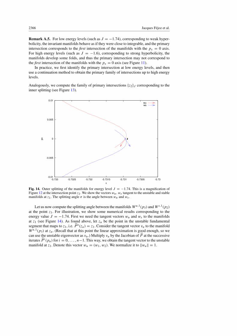
2366 Jacques Fejoz et al.
Remark A.5. For low energy levels (such as J = −1.74), corresponding to weak hyper-bolicity, the invariant manifolds behave as if they were close to integrable, and the primaryintersection corresponds to the first intersection of the manifolds with the px = 0 axis.For high energy levels (such as J = −1.6), corresponding to strong hyperbolicity, themanifolds develop some folds, and thus the primary intersection may not correspond tothe first intersection of the manifolds with the px = 0 axis (see Figure 11).
In practice, we first identify the primary intersection at low energy levels, and thenuse a continuation method to obtain the primary family of intersections up to high energylevels.
Analogously, we compute the family of primary intersections {z2}J corresponding to theinner splitting (see Figure 13).
-0.01
-0.005
0
0.005
0.01
-5.733 -5.7325 -5.732 -5.7315 -5.731 -5.7305 -5.73
px
x
zzzz
wuws
Fig. 14. Outer splitting of the manifolds for energy level J = −1.74. This is a magnification ofFigure 12 at the intersection point z1. We show the vectorswu, ws tangent to the unstable and stablemanifolds at z1. The splitting angle σ is the angle between wu and ws .
Let us now compute the splitting angle between the manifoldsWu,1(p3) andW s,1(p2)
at the point z1. For illustration, we show some numerical results corresponding to theenergy value J = −1.74. First we need the tangent vectors wu and ws to the manifoldsat z1 (see Figure 14). As found above, let zu be the point in the unstable fundamentalsegment that maps to z1, i.e. P n(zu) = z1. Consider the tangent vector vu to the manifoldWu,1(p3) at zu. (Recall that at this point the linear approximation is good enough, so wecan use the unstable eigenvector as vu.) Multiply vu by the Jacobian of P at the successiveiterates P i(pu) for i = 0, . . . , n−1. This way, we obtain the tangent vector to the unstablemanifold at z1. Denote this vector wu = (w1, w2). We normalize it to ‖wu‖ = 1.

Restricted planar three-body problem 2367
-1.5
-1
-0.5
0
0.5
1
1.5
2
2.5
-1.85 -1.8 -1.75 -1.7 -1.65 -1.6 -1.55
s
H
outer
inner
Fig. 15. Splitting angle associated to inner and outer splitting.
Due to reversibility, the vector ws tangent to the stable manifold at z1 is ws =(w1,−w2) (see Figure 14). Notice that we choose the tangent vectors with appropriateorientation, the same as that of the trajectories on the manifolds.
Thus the oriented splitting angle between wu and ws is
σ = 2 arctan2(−w1,−w2),
where arctan2 is the arctangent function of two variables, which uses the signs of the twoarguments to determine the sign of the result.
Finally, we let J vary and, using this procedure, we are able to obtain the splittingangle for energy levels J ∈ [J−, J+] (see Figure 15). The splitting angle is non-zero forall energy values except for a discrete set of them. The splitting angle oscillates aroundzero with decreasing amplitude as J → J−. Numerically, we find that the zeros of thesplitting angle are in the intervals listed in Table 1.
Table 1. Subintervals of J ∈ [J−, J+] containing the zeros of inner splitting (left column) andouter splitting (right column).
inner outer
(−1.695,−1.694) (−1.701,−1.700)(−1.726,−1.725) (−1.731,−1.730)(−1.756,−1.755) (−1.760,−1.759)(−1.781,−1.780) (−1.784,−1.783)(−1.802,−1.801) (−1.805,−1.804)

2368 Jacques Fejoz et al.
Notice that the inner and outer splittings behave similarly. However, they become zeroat different values of J , as seen in Table 1. Thus, when one of the intersections becomestangent, the other one is still transversal, and we can always use one of them for diffusion.
A.4. Accuracy of computations
For small eccentricities, the splitting angle σ becomes very small. We need to check thevalidity of σ , making sure that the size of (accumulated) numerical errors in the compu-tation is smaller than the size of σ .
The smallest splitting angle in Figure 15, corresponding to J− = −1.81, is
σ(J−) = −1.777970294158603× 10⁻⁵.
We check the validity of σ(J−) by recomputing this angle using an alternative numericalmethod. First we compute the intersection of the manifolds Wu,1(p3) and W s,1(p2) withthe horizontal axis defined by
px = j/105 for j ∈ {−2,−1, 1, 2}.
Table 2. Sampling of the manifolds Wu,1(p3) and W s,1(p2) at different values of px , and theirdifference (last column).
px xu xs xu − xs
−0.00002 −5.481541931871417 −5.481541932226887 0.000000000355470−0.00001 −5.481541931790012 −5.481541931967703 0.0000000001776910.00000 −5.481541931822124 −5.481541931822124 0.0000000000000000.00001 −5.481541931967703 −5.481541931790012 −0.0000000001776910.00002 −5.481541932226887 −5.481541931871417 −0.000000000355470
In Table 2 we tabulate the x coordinate of Wu,1(p3) and W s,1(p2) on these axes, andtheir difference d = xu− xs gives the distance between the manifolds. We apply numeri-cal differentiation to the last column of this table, using central differences centered at z1with step sizes 0.00002 and 0.00004, and obtain the values
d1 =d(0.00001)− d(−0.00001)
0.00002= −0.0000177691,
d2 =d(0.00002)− d(−0.00002)
0.00004= −0.0000177735.
Finally, we use Richardson extrapolation and obtain
d = (4d1 − d2)/3 = −0.00001776763333333333.
Thus, using this alternative method, we obtain the splitting angle
σ(J−) = atan(−0.00001776763333333333) = −0.00001776763333146364.
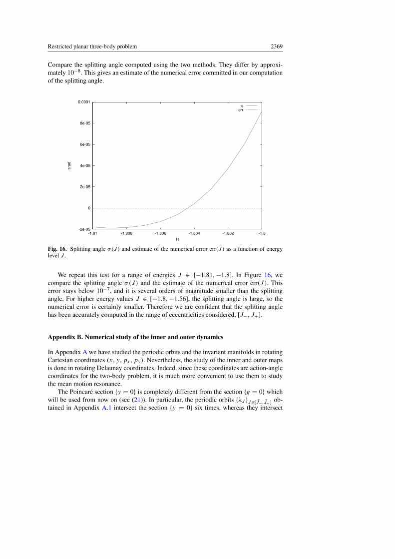
Restricted planar three-body problem 2369
Compare the splitting angle computed using the two methods. They differ by approxi-mately 10−8. This gives an estimate of the numerical error committed in our computationof the splitting angle.
-2e-05
0
2e-05
4e-05
6e-05
8e-05
0.0001
-1.81 -1.808 -1.806 -1.804 -1.802 -1.8
sra
d
H
s
err
Fig. 16. Splitting angle σ(J ) and estimate of the numerical error err(J ) as a function of energylevel J .
We repeat this test for a range of energies J ∈ [−1.81,−1.8]. In Figure 16, wecompare the splitting angle σ(J ) and the estimate of the numerical error err(J ). Thiserror stays below 10−7, and it is several orders of magnitude smaller than the splittingangle. For higher energy values J ∈ [−1.8,−1.56], the splitting angle is large, so thenumerical error is certainly smaller. Therefore we are confident that the splitting anglehas been accurately computed in the range of eccentricities considered, [J−, J+].
Appendix B. Numerical study of the inner and outer dynamics
In Appendix A we have studied the periodic orbits and the invariant manifolds in rotatingCartesian coordinates (x, y, px, py). Nevertheless, the study of the inner and outer mapsis done in rotating Delaunay coordinates. Indeed, since these coordinates are action-anglecoordinates for the two-body problem, it is much more convenient to use them to studythe mean motion resonance.
The Poincare section {y = 0} is completely different from the section {g = 0} whichwill be used from now on (see (21)). In particular, the periodic orbits {λJ }J∈[J−,J+] ob-tained in Appendix A.1 intersect the section {y = 0} six times, whereas they intersect

2370 Jacques Fejoz et al.
-0.4
-0.3
-0.2
-0.1
0
0.1
0.2
0.3
0.4
-6 -5.5 -5 -4.5 -4 -3.5 -3 -2.5 -2 -1.5
px
x
p0
p1
p2
p3
p4
p5
z1 z2
Fig. 17. Energy J = −1.74. Resonance structure in Cartesian coordinates. The axis of symmetryis the horizontal line.
1.9
1.905
1.91
1.915
1.92
1.925
1.93
0 1 2 3 4 5 6
L
l
p0
p1 p2 p3 p4 p5 p6
z1
z2
p0
p1 p2 p3 p4 p5 p6
z1
z2
p0
p1 p2 p3 p4 p5 p6
z1
z2
p0
p1 p2 p3 p4 p5 p6
z1
z2
Fig. 18. Energy J = −1.74. Resonance structure in Delaunay coordinates. The symmetry corre-sponds to l = 0 and l = π and is marked with a vertical line.
{g = 0} seven times. However, we remark that the homoclinic points z1 and z2 lie on thesymmetry axis both in Cartesian and in Delaunay variables (see Figures 17 and 18).

Restricted planar three-body problem 2371
To obtain the intersection of these periodic orbits with {g = 0} we just need to ex-press the 6-periodic points of the Poincare map P obtained in Appendix A.1 in Delaunaycoordinates and then iterate them by the flow of the circular problem expressed in Delau-nay coordinates until they hit the section {g = 0}. We do the same with the homoclinicpoints. In Appendix B.1 we explain how to compute the change of coordinates and thevector field in Delaunay coordinates. Then, in Appendices B.2 and B.3 we study the innerand outer maps of the circular and elliptic problems respectively. Finally, in Appendix B.4we compare the inner and outer maps of the elliptic problem, which leads to Ansatz 3.
B.1. From Cartesian to Delaunay and computation of ∂G1Hcirc
We explain an easy way to obtain rotating Delaunay coordinates from rotating Cartesian(or polar) coordinates in the circular problem. First recall that G can be computed as
G = r(−px sinφ + py cosφ).
The potential µ1Hcirc in Cartesian coordinates only depends on the position (x, y)of the asteroid, and can be easily computed. Then, one can use the equation
J = −1
2L2 −G+ µ1Hcirc
to obtain L. Knowing L and G we can obtain the eccentricity e by
e =
√1−G2/L2.
Using the fact that r = L2(1− e cos u), one can obtain u and from here ` using Kepler’sequation u− e sin u = `. On the other hand, from u we can obtain v using
tanv
2=
√1+ e1− e
tanu
2.
Finally, we can find g using φ = v + g.We devote the rest of this appendix to computing ∂G1Hcirc. The other derivatives of
1Hcirc can be computed analogously. Define
D[r0] = D[r0](r, v, g) =(r2+ r2
0 − 2rr0 cos(v + g))−1/2
.
Then1Hcirc(L, `,G, g) = −(1− µ)D[−µ] − µD[1− µ] −D[0].
Thus by the chain rule it only remains to compute ∂Gr and ∂Gv. First, let us point out that
∂Ge = −G
eL2 =e2− 1eG
.
On the other hand, as ` = u− e sin u, one has
∂eu =sin u
1− e cos u.

2372 Jacques Fejoz et al.
Then, since r(L, e, `) = L2(1− e cos u(e, `)), using
cos v =cos u− e
1− e cos u, (94)
we obtain∂er(L, e, `) = L
2 cos v,
and therefore
∂Gr(L, `,G) = −G cos ve
.
To compute ∂Gv, let us point out that ∂Gv = ∂ev∂Ge. Therefore it only remains to com-pute ∂ev; we obtain it using formula (94) and
sin v =
√1− e2 sin u
1− e cos u.
Then
∂ev =sin v
1− e2 (2+ e cos v),
and therefore
∂Gv = −sin veG
(2+ e cos v).
B.2. Inner and outer dynamics of the circular problem
In this appendix, we numerically compute the inner map F in0 and the outer maps Fout,∗
0of the circular problem, given in Section 2. Recall that to compute these maps we dealwith the extended system given by the Hamiltonian H in (16) with e0 = 0 restricted tothe energy level H = 0, and thus we have I = −J . Then, we consider I ∈ [I−, I+] =[−J+,−J−], where the range [−J+,−J−] is given in (93).
As seen in Section 2.2, the inner map has the form
F in0 :
(I
t
)7→
(I
t + µT0(I )
), (95)
where TJ = 14π + µT0(I ) is the period of the periodic orbit obtained in Ansatz 1 onthe corresponding level of energy J , which now corresponds to an invariant hyperplaneI = constant.
Recall that we computed the periodic orbit λJ as well as its period TJ in Ap-pendix A.1. In particular, Figure 6 shows a plot of the function TJ − 14π = µT0(I ).Notice that the derivative of the function T0(I ) is non-zero for the whole range [I−, I+].This shows that the inner map is a twist map. Moreover, Figure 6 shows that
0 < µT0(I ) < 60µ < π.
Therefore, the function T0(I ) has the properties stated in Lemma 2.

Restricted planar three-body problem 2373
0
50
100
150
200
250
300
350
-1.8 -1.75 -1.7 -1.65 -1.6
H
wf
wb
Fig. 19. The functions ωf(I ) and ωb(I ) involved in the definition of the outer map (96) of thecircular problem as a function of the Jacobi constant J (recall that in the circular problem, I = −J ).
As a test, we have computed the same function T0(I ) using two different methods: firstby computing the period of the periodic orbit, as above; then by computing the integralexpression (38) using numerical integration. The difference in T0(I ) using both methodsis of the order 10−12.
As seen in Section 2.3, the outer maps have the form
Fout,∗0 :
(I
t
)7→
(I
t + µω∗(I )
), ∗ = f, b. (96)
For simplicity, let us only discuss the computation of ωf(I ) (ωb(I ) is computed analo-gously). Recall from Lemma 2.6 that the function ωf(I ) is defined as
ωf(I ) = ωfout(I )+ ω
fin(I ),
where, taking into account that the homoclinic orbit is symmetric with respect to theinvolution (19),
ωfout(I ) = ω
f+(I )− ω
f−(I ) = 2ωf
+(I ) (97)
with
ωf+(I ) = lim
N→∞
(∫ 14Nπ
0
(∂G1Hcirc) ◦ γfI (σ )
−1+ µ(∂G1Hcirc) ◦ γfI (σ )
dσ +NT0(I )
), (98)
ωfin(I ) =
∫−12π
0
(∂G1Hcirc) ◦ λ4I (σ )
−1+ µ(∂G1Hcirc) ◦ λ4I (σ )
dσ. (99)

2374 Jacques Fejoz et al.
To obtain ωf(I ), we compute the integrals (98) and (99) numerically, using a standardalgorithm from the GSL library [GG09]. The integrals are computed within a relativeerror limit 10−9.
The function ∂G1Hcirc involved in both integrals is given explicitly in Appendix B.1.The integral ωf
in(I ) is evaluated on a periodic trajectory λ4I (σ ) of the reduced circular
problem (namely, with reparameterized time, see (30)) with initial condition p4, a fixedpoint of the Poincare map P7
0 . The integral ωf+(I ) is evaluated on a homoclinic trajectory
γ fI (σ ) of the reduced circular problem with initial condition z2, the primary homoclinic
point corresponding to the inner splitting found in Appendix A.3.
1e-08
1e-07
1e-06
1e-05
0.0001
0.001
0.01
0.1
1
0 5 10 15 20 25 30 35 40
d
N
-1.85
-1.8
-1.75
-1.7
-1.65
-1.6
-1.55
Fig. 20. Exponential decay of the function dist+ as a function of N (multiples of the period) fordifferent energy levels. The energy levels J ∈ [J−, J+] are color-coded.
Next we make a couple of important remarks about the numerical computation of theintegral ωf
+(I ). The key point is that the homoclinic orbit γ fI was already computed in
Appendix A.3 with high accuracy, and we can exploit this information here. Recall thatthe primary homoclinic point z2 was obtained as the n-th iterate of a point zu in the localfundamental segment lu under the Poincare map:
z2 = {P70 }n(zu). (100)
Moreover, recall that the point zu was chosen to be suitably close to the fixed point p3 foreach energy level J (see Remark A.3).
Notice that the integral ωf+(I ) is defined by a limit as N →∞, i.e. as the homoclinic
orbit γ fI (σ ) asymptotically approaches the periodic orbit λ3
I (σ ) in forward time (see (39)).Numerically, of course, we should stop integrating at an upper endpoint N large enoughsuch that the integral converges. In practice, we choose the upper endpoint N = N(I)

Restricted planar three-body problem 2375
to be the number of iterates n = n(I) in (100). This means that we evaluate the integralalong the homoclinic trajectory γ f
I (σ ) until it reaches the point zu, which is suitably closeto the periodic orbit.
Notice also that integrating the homoclinic trajectory γ fI (σ ) forwards in the reduced
system means integrating it backwards along the unstable manifold in the original sys-tem. This is numerically unstable, since numerical errors grow exponentially. In practice,we rewrite the integral (98) using the change of variables σ = σ − 14Nπ so that thehomoclinic trajectory is integrated forwards along the unstable manifold, starting fromthe point zu.
The computed values of the functions ωf(I ) and ωb(I ) are shown in Figure 19. Notethat they are plotted as a function of the Jacobi constant J instead of as a function of I ,so that they can be compared with Figure 6, where we have plotted µT0(I ) = TJ − 14πas a function of J .
To test the computation of the function ωf+, we directly verify the definition of the
outer map in 2.3. Let z2 = (Lh, `h,Gh, 0) be the primary homoclinic point, and letp3 = (Lp, `p,Gp, 0) be the periodic point. Given a point (Lh, `h,Gh, 0, I, t) in theextended circular problem, we check that it is forward asymptotic (in the reparameterizedtime) to the point (Lp, `p,Gp, 0, I, t + ωf
+(I )), where t ∈ T is arbitrary. Thus we checkthat
dist+(s) = |80{s, (Lh, `h,Gh, 0, I, t)} −80{s, (Lp, `p,Gp, 0, I, t +ωf+(I ))}|
s→∞−−−→ 0
with exponential decay.The result of the test is shown in Figure 20 for values of the energy J ∈ [J−, J+]
(recall that J = −I ). Notice that the vertical axis is in logarithmic scale. Let s = 14Nπ .We plot the distance dist+ as a function of N (multiples of the period). The test showsexponential decay of the distance function for all energy values, i.e. straight lines in theplot.
Recall that the periodic orbits λ3,4I (s) become more hyperbolic as the energy I de-
creases. Thus, the rate of exponential convergence between the homoclinic and the pe-riodic trajectory also increases, i.e. the straight lines have increasing slope in the plot.As explained above, the length of integration N = N(I) along the homoclinic orbit issuitably chosen for each energy level. For I → I−, there is exponential decay up to times = 40 · (14π) ≈ 1760.
B.3. Inner and outer dynamics of the elliptic problem
In this appendix, we numerically compute the first orders in e0 of the inner map F ine0
andthe outer maps Fout,∗
e0 of the elliptic problem, given in Section 3. In order to compare theinner and outer dynamics of the elliptic problem through Lemma 4.2, only some specificterms in the expansions of the inner and outer maps are necessary. Namely, we only needto compute the term A1 in the expansion of the inner map (61), and the terms B∗ in theexpansion of the outer maps (72).

2376 Jacques Fejoz et al.
-0.0005
-0.00045
-0.0004
-0.00035
-0.0003
-0.00025
-0.0002
-0.00015
-0.0001
-5e-05
0
5e-05
-2.05 -2 -1.95 -1.9 -1.85 -1.8 -1.75 -1.7 -1.65 -1.6 -1.55
A
H
reXXXXXX
imXXXXXX
Fig. 21. The function A+1 (I ) (real and imaginary parts) involved in the definition of the innermap (61) of the elliptic problem as a function of the energy of the system in rotating coordinates H .Recall that H = −I .
Recall from Section 3.4 that A1 can be split as
A1(I, t) = A+
1 (I )eit+ A−1 (I )e
−it .
Since A+1 and A−1 are complex conjugate, it is only necessary to compute one of them.Let us compute the positive harmonic,
A+1 (I ) = −iµ
∫−14π
0
1H1,+ell ◦ λ
3I (σ )
−1+ µ∂G1Hcirc ◦ λ3I (σ )
eiλ3I (σ ) dσ. (101)
Notice that the denominator is the same one used in the previous section for the inner andouter dynamics of the circular problem. Next we give the numerator i1H 1,+
ell explicitly.Let
1H 1ell(L, `,G, g, t) = −
1− µµ
B1
(−r(L, `,G)
µ, v(L, `,G), g, t
)−
µ
1− µB1
(r(L, `,G)
1− µ, v(L, `,G), g, t
),
where B1 is the function defined in Lemma 3.4. Then it is straightforward to see that
1H1,+ell (l, L, g,G) = −
1− µµ
B+1(−r(L, `,G)
µ, v(L, `,G), g
)−
µ
1− µB+1(r(L, `,G)
1− µ, v(L, `,G), g
), (102)

Restricted planar three-body problem 2377
-0.0005
0
0.0005
0.001
0.0015
0.002
0.0025
-1.8 -1.75 -1.7 -1.65 -1.6
H
reBfXXXXXX
imBfXXXXXX
reBbXXXXXX
imBbXXXXXX
Fig. 22. The functions Bf,+ and Bb,+ (real and imaginary parts) involved in the definition of theouter map (72) of the elliptic problem.
where
B+1 (r, v, g) = −1− r cos(v + g)− i2r sin(v + g)
213(r, v + g).
The computed value of the functionA+1 is shown in Figure 21. We plot it as a functionof the energy of the elliptic problem in rotating coordinates H in (15). Recall that sincewe are working in the energy level H = 0 of the extended Hamiltonian H in (16), wehave I = −H .
For the outer map, we compute the functions B∗(I ). Similarly to A1, it is only nec-essary to compute the positive harmonics B∗,+. Recall from Lemma 3.9 that the positiveharmonics Bf,+(I ) and Bb,+(I ) are defined as
Bf,+(I ) = Bf,+out (I )+ B
f,+in (I )eiµω
fout(I ),
Bb,+(I ) = Bb,+in (I )+ B
b,+out (I )e
iµωbin(I ),
(103)
where ωfout and ωb
in were obtained in Appendix B.2. To obtain B∗,+out and B∗,+in , we com-pute the integrals (74)–(76) numerically, using the same techniques as in the previousAppendix B.2. In particular, the integrands of the Melnikov integrals (74) and (75), byconstruction, decay exponentially as T →±∞ and we take the same approximate limitsof integration ±14πN where N = N(I) is the constant considered in Appendix B.2.
The computed values of the functions Bf,+(I ) and Bb,+(I ) are shown in Figure 22.

2378 Jacques Fejoz et al.
B.4. Comparison of the inner and outer dynamics of the elliptic problem
Finally, we verify the non-degeneracy condition
B∗,±(I) 6= 0 for I ∈ D∗ (104)
stated in Lemma 4.2, which implies the existence of a transition chain of tori. Since B∗,+
and B∗,− are complex conjugate, it is only necessary to compute one of them. Let uscompute the positive harmonic,
B∗,+(I) = B∗,+(I)− eiµω∗(I)
− 1eiµT0(I) − 1
A+1 (I).
All the functions involved in the expression above are known: T0 and ω∗ are obtained inAppendix B.2 and A+1 and B∗,+ are obtained in Appendix B.3.
The computed values of the functions Bf,+ and Bb,+ are shown in Figure 23. Thus,we see that the functions B∗,+ are not identically zero. This justifies Ansatz 3.
-0.0005
0
0.0005
0.001
0.0015
0.002
0.0025
0.003
0.0035
0.004
-1.8 -1.75 -1.7 -1.65 -1.6
H
reBfXXXXXX
imBfXXXXXX
reBbXXXXXX
imBbXXXXXX
Fig. 23. The functions Bf,+ and Bb,+ (real and imaginary parts).
Remark B.1. Figure 23 also shows that Bf,+ and Bb,+ are almost identical, which issurprising to the authors. However, this fact is not relevant for the argument in Lemma 4.2;we only need that these functions do not vanish identically.

Restricted planar three-body problem 2379
Appendix C. The Main Result for the 3 : 1 resonance: instabilities in the Kirkwoodgaps
We devote this appendix to showing how the proof of Theorem 1 in Sections 2–4 can beadapted to deal with the 3 : 1 resonances. First, we state a more rigorous version of MainResult (3 : 1).
Theorem 5. Assume Ansatze 4–6. Then there exists e∗0 > 0 such that for 0 < e0 < e∗0 ,there exist T > 0 and an orbit of the Hamiltonian (16) which satisfy
G(0) > 0.56 and G(T ) < 0.32,
whereas|L(t)− 3−1/3
| ≤ 100µ for t ∈ [0, T ].
Ansatze 4 and 5 are stated in Appendix C.1 and Ansatz 6 is stated in Appendix C.2. Theyare analogous to Ansatze 1–3 but refer to the 3 : 1 resonance instead of the 1 : 7 one. Toprove this theorem, we consider the Hamiltonian (16) and we study the resonance
˙ ∼ 3 and g ∼ −1. (105)
As for the 1 : 7 resonance, without loss of generality, we take H = 0 and we look for alarge drift in I which, L being almost constant, implies a big drift in G.
C.1. The circular problem
We first study the circular problem (18), close to the resonance 3−1 ˙+ g ∼ 0. We assumethe following Ansatz. It has been verified numerically (see Appendix C.3). It replicatesAnsatz 1.
Ansatz 4. Consider the Hamiltonian (18) with µ = 10−3. Then, at each energy levelJ ∈ [J−, J+] = [−1.6,−1.3594], there exists a hyperbolic periodic orbit λJ =(LJ (t), `J (t),GJ (t), gJ (t)) of period TJ which satisfies
|TJ − 2π | < 15µ,
and is smooth with respect to J , and
|LJ (t)− 3−1/3| < 100µ for all t ∈ R.
Each λJ has two branches of stable and unstable invariant manifolds W s,j (λJ ) andWu,j (λJ ), j = 1, 2. Then, for each J ∈ [J−, J+] either W s,1(λJ ) and Wu,1(λJ ) orW s,2(λJ ) and Wu,2(λJ ) intersect transversally.
Note that since now Jupiter is slower than the asteroid, the period of these periodic orbitsis approximately the period of Jupiter instead of the period of the asteroid. For the Ex-tended Circular Problem given by the Hamiltonian (16) with e0 = 0, the periodic orbitsobtained in Ansatz 4 become invariant 2-dimensional tori which lie on the hyperplanesI = constant for any
I ∈ [I−, I+] = [−J+,−J−] = [1.3594, 1.6].

2380 Jacques Fejoz et al.
Corollary C.1. Assume Ansatz 4. Then the Hamiltonian (16) with µ = 10−3 and e0 = 0has an analytic normally hyperbolic invariant 3-dimensional manifold 30, which is foli-ated by 2-dimensional invariant tori.
Moreover, 30 has two branches of stable and unstable invariant manifolds, which wecall W s,j (30) and Wu,j (30), j = 1, 2. Then, in the invariant planes I = constant, foreach I ∈ [I−, I+] either W s,1(30) and Wu,1(30) or W s,2(30) and Wu,2(30) intersecttransversally.
For the analysis of the 3 : 1 resonance it is more convenient to consider the global Poincaresection {` = 0} instead of the section {g = 0} considered in Section 2, since now theasteroid moves faster than Jupiter. We consider the map
P0 : {` = 0} → {` = 0}, (106)
induced by the flow associated to the Hamiltonian (16) with e0 = 0. Now the intersectionof the cylinder 30 with the section {` = 0} is formed by three cylinders 3j0 , j = 0, 1, 2:
30 ∩ {` = 0} = 30 =
2⋃j=0
3j
0. (107)
As a whole,⋃2j=0 3
j
0 is a normally hyperbolic invariant manifold for the Poincare
map P0, whereas each 3j0 is a normally hyperbolic invariant manifold for P30 . These
cylinders have a natural system of coordinates, which we use to study the inner and outerdynamics on them. We work with 31
0 and 320 since in each invariant plane I = constant
they are connected by at least one heteroclinic connection (of P30 ) which is symmetric
with respect to the involution (19). As before, we call it a forward heteroclinic orbit if itis asymptotic to 31
0 in the past and 320 in the future and a backward heteroclinic orbit if
it is asymptotic to 320 in the past and to 31
0 in the future. We denote by Df⊂ [I−, I+],
where f stands for forward, the subset of [I−, I+] where Wu(310) and W s(32
0) inter-sect transversally, and by Db
⊂ [I−, I+], where b stands for backward, the subset of[I−, I+] where W s(31
0) and Wu(320) intersect transversally. By Corollary C.1 we have
Df∪Db
= [I−, I+].
Corollary C.2. Assume Ansatz 4. Then the Poincare map P30 defined in (106), which is
induced by the Hamiltonian (16) with µ = 10−3 and e0 = 0, has three analytic nor-mally hyperbolic invariant manifolds 3j0 , j = 0, 1, 2. They are foliated by 1-dimensionalinvariant curves. Moreover, there exist analytic functions Gj0 : [I−, I+] ×T→ (R×T)3,
Gj0 (I, t) =(Gj,L0 (I ), 0,Gj,G0 (I ),Gj,g0 (I ), I, t
),
that parameterize 3j0 ,
3j
0 = {Gj
0 (I, t) : (I, t) ∈ [I−, I+] × T}.

Restricted planar three-body problem 2381
The associated invariant manifoldsWu(310) andW s(33
0) intersect transversally providedI ∈ Df; and W s(31
0) and Wu(320) intersect transversally provided I ∈ Db. Moreover,
one of the points of these intersections belongs to the symmetry axis of (19). Denote by0∗0 , ∗ = f, b, these intersections. Then there exist analytic functions
C∗0 : Dj× R→ (R× T)3, (I, t) 7→ C∗0 (I, t), ∗ = f, b,
which parameterize them:
0∗0 ={C∗0 (I, t) =
(C∗,L0 (I ), 0, C∗,G0 (I ), C∗,g0 (I ), I, t
): (I, t) ∈ D∗ × T
}, ∗ = f, b.
Corollary C.1 gives global coordinates (I, t) for each cylinder 3j0 . These coordinates aresymplectic with respect to the canonical symplectic form �0 = dI ∧ dt . We consider theinner and the two outer maps in the cylinder 31
0.
The inner map. The inner map F in0 : 3
10 → 31
0 is defined as the Poincare map P30
restricted to the symplectic invariant submanifold 310. It is of the form
F in0 :
(I
t
)7→
(I
t + µT0(I )
), (108)
where the function T0 is such that 2π+µT0(I ) is the period of the periodic orbit obtainedin Ansatz 4 on the corresponding energy surface. We assume the following Ansatz, whichasserts that this map is a twist map (see the corresponding Ansatz 2). It has been verifiednumerically (see Appendix C.3).
Ansatz 5. The function T0(I ) satisfies
∂IT0(I ) 6= 0 for I ∈ [I−, I+].
Therefore, the analytic symplectic inner map F in0 is a twist map. Moreover,
0 < µT0(I ) < π.
The outer map. Proceeding as in Section 2.3, we define the outer map for the circularproblem at the 3 : 1 resonance. Recall that it has been defined as the composition of themap given by Definition 2.3 and a suitable power of the Poincare map P0 restricted to thecylinders 3j0 . For the 3 : 1 resonance, we consider the outer maps Fout,∗
0 , ∗ = f, b, whichconnect 31
0 to itself and are defined as
Fout,f0 = P2
0 ◦ Sf: 31
0 → 310, Fout,b
0 = Sb◦ P0 : 3
10 → 31
0,
where Sf is the outer map which connects 310 and 32
0 through Wu(310) ∩W
s(320), and
Sb is the outer map which connects 320 and 31
0 through Wu(320) ∩W
s(310). Recall that
we are abusing notation since the forward and backward outer maps are only definedprovided I ∈ Df and I ∈ Db respectively, and not in the whole cylinder 31
0.

2382 Jacques Fejoz et al.
As for the 1 : 7 case, these maps are of the form
Fout,∗0 :
(I
t
)7→
(I
t + µω∗(I )
), ∗ = f, b. (109)
Since we want to compute these outer maps using flows, we need to reparameterize timein the vector field associated to the Hamiltonian (16) with e0 = 0, so that it preserves thesection {` = 0}. We consider the following vector field, which corresponds to identifyingthe variable ` with time:
d
ds` = 1,
d
dsL = −
∂`H
L−3 + µ∂L1Hcirc,
d
dsg =−1+ µ∂G1Hcirc
L−3 + µ∂L1Hcirc,
d
dsG = −
∂gH
L−3 + µ∂L1Hcirc,
d
dst =
1L−3 + µ∂L1Hcirc
,d
dsI = 0,
(110)
where H is the Hamiltonian (16) with e0 = 0. Notice that now we are not changing thetime direction, as happened in the 1 : 7 resonance. We refer to this system as a reducedcircular problem. Recall that we denote by 8circ
0 the flow associated to the (L, `,G, g)components of equation (30) (which are independent of t and I ). We use it to derive theformulas for the outer map. Let
γ ∗I (σ ) = 8circ0 {σ, (C∗,L0 (I ), 0, C∗,G0 (I ), C∗,g0 (I ))}, ∗ = f, b,
λjI (σ ) = 8
circ0 {σ, (G
j,L
0 (I ), 0,Gj,G0 (I ),Gj,g0 (I ))}(111)
be trajectories of the circular problem. Then one can see that the functions ωf,b(I ) in-volved in the definition of the outer maps in (109) can be defined as
ω∗(I ) = ω∗out(I )+ ω∗
in(I ),
whereω∗out(I ) = ω
∗+(I )− ω
∗−(I ) (112)
with
ω∗+(I ) = limN→∞
(∫ 6Nπ
0
(µ−1(3−L−3)−∂L1Hcirc)◦γ∗
I (σ )
3(L−3+µ∂L1Hcirc)◦γ∗
I (σ )dσ +NT0(I )
),
ω∗−(I ) = limN→−∞
(∫ 6Nπ
0
(µ−1(3−L−3)−∂L1Hcirc)◦γ∗
I (σ )
3(L−3+µ∂L1Hcirc)◦γ∗
I (σ )dσ +NT0(I )
), ∗ = f, b,
(113)
and
ωfin(I ) =
∫ 4π
0
(µ−1(3− L−3)− ∂L1Hcirc) ◦ λ2I (σ )
3(L−3 + µ∂L1Hcirc) ◦ λ2I (σ )
dσ,
ωbin(I ) =
∫ 2π
0
(µ−1(3− L−3)− ∂L1Hcirc) ◦ λ1I (σ )
3(L−3 + µ∂L1Hcirc) ◦ λ1I (σ )
dσ,
(114)
where T0(I ) is the function in (108). Recall that along periodic and homoclinic orbits,3− L−3
∼ µ.

Restricted planar three-body problem 2383
C.2. The elliptic problem
We now study the elliptic problem. Reasoning as for the 1 : 7 resonance, for e0 smallenough the system associated to the Hamiltonian (16) has a normally hyperbolic invariantcylinder 3e0 , which is e0-close to 30 given in Corollary 2.1. Analogously, the Poincaremap
Pe0 : {` = 0} → {` = 0}
associated to the flow of (16) and the section {` = 0} has a normally hyperbolic invariantcylinder 3e0 = 3e0 ∩ {` = 0}. Moreover, it is formed by three connected components3je0 , j = 0, 1, 2, which are e0-close to the cylinders 3je0 obtained in Corollary C.2 and
have natural coordinates (I, t) as happened for the circular case.We look for perturbative expansions of the inner and outer maps. For the 3 : 1 reso-
nances they are computed using the new reduced elliptic problem
d
ds` = 1,
d
dsL = −
∂`H
L−3+µ∂L1Hcirc+µe0∂L1Hell,
d
dsg =
∂GH
L−3+µ∂L1Hcirc+µe0∂L1Hell,
d
dsG = −
∂gH
L−3+µ∂L1Hcirc+µe0∂L1Hell,
d
dst =
1L−3+µ∂L1Hcirc+µe0∂L1Hell
,d
dsI = −
µe0∂t1Hell
L−3+µ∂L1Hcirc+µe0∂L1Hell,
(115)which is a perturbation of (110).
For the elliptic problem, the coordinates (I, t) are symplectic not with respect to thecanonical symplectic form dI ∧ dt but with respect to a symplectic form
�je0 =
(1+ e0a
j
1 (I, t)+ e20aj
2 (I, t)+ e30aj≥(I, t)
)dI ∧ dt (116)
with certain functions ajk : [I−, I+] × T→ R which satisfy
N (a31) = {±1}, N (a3
2) = {0,±1,±2}
(see (84) for the definition of N and Corollary 3.8 for the corresponding result for the1 : 7 resonance).
In the invariant cylinder 31e0
, one can define inner and outer maps as we have donein 31
0 for the circular problem. We proceed as in Section 3 for the 1 : 7 resonance.
The inner map. We first study the inner map. As for the circular problem, it is defined bythe map P3
e0in (41) restricted to the normally hyperbolic invariant manifold 31
e0. For e0
small enough, proceeding as in the proof of Lemma 3.7, one can see that it is of the form
F ine0:
(I
t
)7→
(I + e0A1(I, t)+ e
20A2(I, t)+O(e3
0)
t + µT0(I )+ e0T1(I, t)+ e20T2(I, t)+O(e3
0)
)(117)

2384 Jacques Fejoz et al.
with functions A1, A2, T1, and T2 satisfying
N (A1) = {±1}, N (A2) = {0,±1,±2}, (118)N (T1) = {±1}, N (T2) = {0,±1,±2}. (119)
Thus, A1 can be split as
A1(I, t) = A+
1 (I )eit+ A−1 (I )e
−it .
Moreover, the Fourier coefficients are defined as
A±1 (I ) = ∓iµ
∫ 6π
0
1H1,±ell ◦ λ
1I (σ )
L−3 + µ∂G1Hcirc ◦ λ1I (σ )
e±iλ1I (σ ) dσ,
where the functions 1H 1,±ell are defined as
1H 1ell(L, `,G, g, t) = 1H
1,+ell (L, `,G, g)e
it+1H
1,±ell (L, `,G, g)e
−it ,
and λ1I (σ ) has been defined in (111). Finally, λ1
I (σ ) is defined as
λ1I (σ ) = 80{σ, (G1,L
0 (I ),G1,`0 (I ),G1,G
0 (I ), 0)}, (120)
where G30 has been introduced in Corollary C.2 and
80{s, (L, `,G, g)} = t +
∫ s
0
1
L−3 + µ∂L1Hcirc(8circ0 {σ, (L, `,G, g)})
dσ. (121)
The function 80 is analogous to the corresponding function for the 1 : 7 resonance, de-fined in (36).
The outer map. We now study the outer maps
Fout,∗e0: 31
e0→ 31
e0, ∗ = f, b, (122)
for e0 > 0. Thanks to Ansatz 4, we know that for e0 small enough, there exist transver-sal intersections of the invariant manifolds of 31
e0and 32
e0. Thus, we can proceed as in
Section 2.3 to define the outer maps Foute0
for the 3 : 1 resonance and we study them as aperturbation of the outer maps of the circular problem given in (109). We use the reducedelliptic problem defined in (115) and we compute the first order of the outer maps in e0.To this end, we use the notation γ f,b
I (σ ) and λ1,2I (σ ) defined in (111). Analogously we
define the corresponding t-component of the flow as
γ ∗I (σ ) = 80{σ, (C∗,L0 (I ), C∗,`0 (I ), C∗,G0 (I ), 0)}, ∗ = f, b,
λjI (σ ) = 80{σ, (Gj,L0 (I ),Gj,`0 (I ),Gj,G0 (I ), 0)}, j = 1, 2,
(123)
where C∗0 and Gj0 have been given in Corollary C.2 and 80 in (121).
Restricted planar three-body problem 2385
Lemma C.3. The outer map defined in (122) has the following expansion with respectto e0:
Fout,∗e0:
(I
t
)7→
(I + e0(B
∗,+(I )eit + B∗,−(I )e−it )+O(e20)
t + µω∗(I )+O(e0)
), ∗ = f, b. (124)
Moreover, the functions B∗,±(I ) can be defined as
Bf,±(I ) = Bf,±out (I )+ B
f,±in (I )e±iµω
fout(I ),
Bb,±(I ) = Bb,±in (I )+ B
b,±out (I )e
±iµωbin(I ),
(125)
where ωfout(I ) and ωb
in(I ) are the functions defined in (33) and (35) respectively and
Bf,±out (I ) =±iµ lim
T→∞
∫ T
0
(1H
1,±ell ◦ γ
fI (σ )
L−3 + µ∂L1Hcirc ◦ γfI (σ )
e±iγfI (σ )
−1H
1,±ell ◦ λ
1I (σ )
L−3 + µ∂L1Hcirc ◦ λ1I (σ )
e±i(λ1I (σ )+µω
f+(I ))
)dσ
∓ iµ limT→−∞
∫ T
0
(1H
1,±ell ◦ γ
fI (σ )
L−3 + µ∂L1Hcirc ◦ γfI (σ )
e±iγfI (σ )
−1H
1,±ell ◦ λ
2I (σ )
L−3 + µ∂L1Hcirc ◦ λ2I (σ )
e±i(λ2I (σ )+µω
f−(I ))
)dσ, (126)
Bb,±out (I ) =±iµ lim
T→∞
∫ T
0
(1H
1,±ell ◦ γ
bI (σ )
L−3 + µ∂L1Hcirc ◦ γbI (σ )
e±iγbI (σ )
−1H
1,±ell ◦ λ
2I (σ )
L−3 + µ∂L1Hcirc ◦ λ2I (σ )
e±i(λ2I (σ )+µω
b+(I ))
)dσ
∓ iµ limT→−∞
∫ T
0
(1H
1,±ell ◦ γ
bI (σ )
L−3 + µ∂L1Hcirc ◦ γbI (σ )
e±iγbI (σ )
−1H
1,±ell ◦ λ
1I (σ )
L−3 + µ∂L1Hcirc ◦ λ1I (σ )
e±i(λ1I (σ )+µω
b−(I ))
)dσ, (127)
Bf,±in (I ) = ∓iµ
∫ 4π
0
1H1,±ell ◦ λ
2I (σ )
L−3 + µ∂L1Hcirc ◦ λ2I (σ )
e±iλ2I (σ ) dσ,
Bb,±in (I ) = ∓
∫ 2π
0
1H1,±ell ◦ λ
1I (σ )
L−3 + µ∂L1Hcirc ◦ λ1I (σ )
e±iλ1I (σ ) dσ
(128)
where
1H1,±ell (`, L, g,G, t) = 1H
1,±ell (`, L, g,G)e
it+1H
1,±ell (`, L, g,G)e
−it
has been defined in Corollary 3.5 and ω∗± have been defined in (113).

2386 Jacques Fejoz et al.
Existence of diffusing orbits. The last step to prove the existence of diffusing orbits canbe done analogously to what has been done in Section 4 for the 1 : 7 resonance. Namely,we just need to obtain a change of coordinates (I, t) = (I, τ )+ e0ϕ(I, τ ) which
• straightens the symplectic form �1e0
(see (116)) into �0 = dI ∧ dτ ;• flattens the inner map in the I -direction.
This is summarized in the next lemma, which merges the corresponding Lemmas 4.1 and4.2 for the 1 : 7 resonance.
Lemma C.4. There exists a change of variables e0-close to the identity,
(I, t) = (I, τ )+ e0ϕ(I, τ ),defined on 31
e0, which:
• transforms the symplectic form �1e0
into the canonical form �0 = dI ∧ dτ ;• transforms the inner map F in
e0in (117) into
F ine0:
(Iτ
)7→
(I +O(µe3
0)
τ + µT0(I)+ e20T2(I)+O(µe3
0).
); (129)
• transforms the outer maps Fout,fe0 and Fout,b
e0 in (124) into
Fout,∗e0:
(Iτ
)7→
(I + e0B
∗(I, τ )+O(µe20)
τ + µω∗(I)+O(µe0)
), ∗ = f, b, (130)
whereB∗(I, τ ) = B∗,+(I)eiτ + B∗,−(I)e−iτ
with
B∗,±(I) = B∗,±(I)− e±iµω∗(I)
− 1e±iµT0(I) − 1
A±1 (I).
To ensure the existence of transition chains of tori, we need to assume the followingAnsatz.
Ansatz 6. The functions B∗,± defined in Lemma C.4 satisfy
B∗,±(I) 6= 0 for I ∈ D∗,where D∗ are the domains considered in Corollary C.2.
With this Ansatz, and also Ansatze 4 and 5, we can proceed as in Section 4 to prove theexistence of a transition chain of tori and of orbits shadowing such a chain.
C.3. Numerical study of the 3 : 1 resonance
In this section, we briefly describe our numerical analysis of the 3 : 1 resonance. In par-ticular, we verify Ansatze 4–6 numerically.
The numerical methodology used for the 3 : 1 resonance is analogous to the 1 : 7 reso-nance. Cartesian rotating coordinates are used for the computation of the hyperbolic struc-ture of the circular problem (normally hyperbolic invariant cylinder, stable and unstable
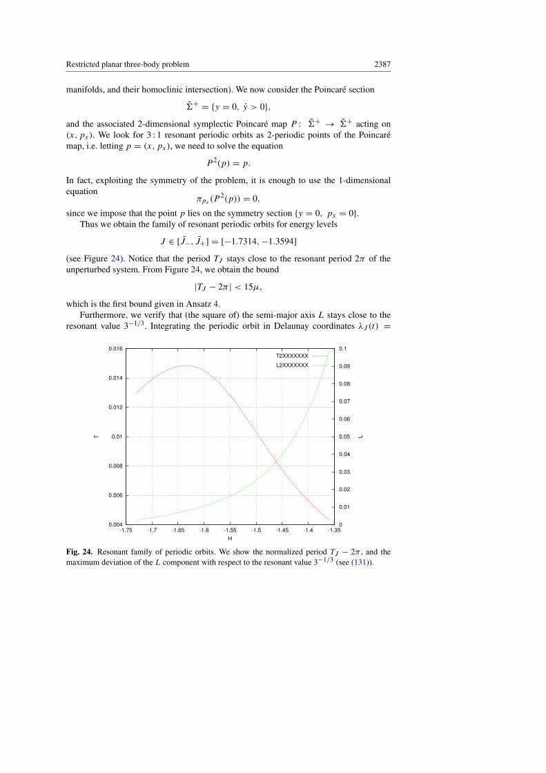
Restricted planar three-body problem 2387
manifolds, and their homoclinic intersection). We now consider the Poincare section
6+ = {y = 0, y > 0},
and the associated 2-dimensional symplectic Poincare map P : 6+ → 6+ acting on(x, px). We look for 3 : 1 resonant periodic orbits as 2-periodic points of the Poincaremap, i.e. letting p = (x, px), we need to solve the equation
P 2(p) = p.
In fact, exploiting the symmetry of the problem, it is enough to use the 1-dimensionalequation
πpx (P2(p)) = 0,
since we impose that the point p lies on the symmetry section {y = 0, px = 0}.Thus we obtain the family of resonant periodic orbits for energy levels
J ∈ [J−, J+] = [−1.7314,−1.3594]
(see Figure 24). Notice that the period TJ stays close to the resonant period 2π of theunperturbed system. From Figure 24, we obtain the bound
|TJ − 2π | < 15µ,
which is the first bound given in Ansatz 4.Furthermore, we verify that (the square of) the semi-major axis L stays close to the
resonant value 3−1/3. Integrating the periodic orbit in Delaunay coordinates λJ (t) =
0.004
0.006
0.008
0.01
0.012
0.014
0.016
-1.75 -1.7 -1.65 -1.6 -1.55 -1.5 -1.45 -1.4 -1.35
0
0.01
0.02
0.03
0.04
0.05
0.06
0.07
0.08
0.09
0.1
T L
H
T2XXXXXXX
L2XXXXXXX
Fig. 24. Resonant family of periodic orbits. We show the normalized period TJ − 2π , and themaximum deviation of the L component with respect to the resonant value 3−1/3 (see (131)).

2388 Jacques Fejoz et al.
(LJ (t), `J (t),GJ (t), gJ (t)) over one period TJ , we compute the quantity
Lmax(J ) = maxt∈[0,TJ )
|LJ (t)− 3−1/3|. (131)
The function Lmax(J ) is plotted in Figure 24. Notice that we obtain the bound
|LJ (t)− 3−1/3| < 100µ
for all t ∈ R and J ∈ [J−, J+], which is the second bound given in Ansatz 4.To determine the stability of the periodic orbits, we now compute the eigenvalues λ
and λ−1 of DP 2(p). Figure 25 shows the characteristic exponent ln(λ) as a function ofenergy. The family of periodic orbits is hyperbolic in the interval [J−, J+], although thestrength of hyperbolicity is weaker than in the 1 : 7 resonance (cf. Figure 7).
The stable and unstable invariant manifolds of the periodic orbits are computed usingthe same methodology explained for the 1 : 7 resonance. In particular, we switch to thenew Poincare section
6− = {y = 0, y < 0}in order to have the homoclinic points lying on the symmetry axis. For illustration, weshow the result corresponding to the energy value J = −1.3594 in Figure 26. The man-ifolds intersect transversally at the homoclinic points z1 (outer splitting) and z2 (innersplitting), as we will show below.
Next we compute the splitting angle between the invariant manifolds at the homoclinicpoints. We will restrict the range of energy values to
J ∈ [J−, J+] = [−1.6,−1.3594], (132)
0
0.1
0.2
0.3
0.4
0.5
0.6
0.7
0.8
0.9
-1.75 -1.7 -1.65 -1.6 -1.55 -1.5 -1.45 -1.4 -1.35
lu
H
Fig. 25. Characteristic exponent ln(λ) as a function of energy level J (the other exponent is− ln(λ)).

Restricted planar three-body problem 2389
-3
-2
-1
0
1
2
3
-0.08 -0.075 -0.07 -0.065 -0.06 -0.055 -0.05 -0.045 -0.04
px
x
p0
p1
z1z2
Fig. 26. Invariant manifolds of the fixed points p0 and p1 for energy level J = −1.3594.
or equivalently the range of eccentricities to e ∈ [e−, e+] = [0.59, 0.91]. This is therange where we can validate the accuracy of our computations (see Appendix A.4). Belowe− = 0.59, the splitting size becomes comparable to the numerical error that we commitin double precision arithmetic.
Remark C.5. In contrast with the 1 : 7 resonance, now the manifolds stay close to the in-tegrable situation for the whole range of energies, i.e. they meet with small splitting angleas we will show below. Thus for the 3 : 1 resonance there is no difficulty in identifying theprimary family of homoclinic points (cf. Remark A.5).
Using the same methodology as for the 1 : 7 resonance, we are able to obtain the splittingangle for energy levels J ∈ [J−, J+] (see Figure 27). Numerically, we find that the zerosof the splitting angle are contained in the intervals listed in Table 3. As seen from thetable, the inner and outer splittings become zero at different values of J . Thus, when oneof the intersections becomes tangent, the other one is still transversal, and we can alwaysuse one of them for diffusion.
Table 3. Subintervals of J ∈ [J−, J+] containing the zeros of inner splitting (left column) andouter splitting (right column).
inner outer(−1.453,−1.451) (−1.477,−1.475)(−1.537,−1.535) (−1.553,−1.551)(−1.593,−1.591)

2390 Jacques Fejoz et al.
-0.00012
-0.0001
-8e-05
-6e-05
-4e-05
-2e-05
0
2e-05
4e-05
6e-05
8e-05
-1.7 -1.65 -1.6 -1.55 -1.5 -1.45 -1.4 -1.35
s
H
inner
outer
Fig. 27. Splitting angle associated to inner and outer splitting.
Again, we check the validity of σ(J−) by computing this splitting angle using twodifferent numerical methods and comparing the results. They differ by less than 10−10,which gives an estimate of the total numerical error.
Recall that the study of the inner and outer maps is done in rotating Delaunay co-ordinates. As explained in Appendix C, for the analysis of the 3 : 1 resonance it is con-venient to consider the Poincare section {` = 0}. Thus, we transform the hyperbolicstructure of the circular problem from Cartesian to Delaunay coordinates as explained inAppendix B.1 (see Figure 28).
First we compute the inner map F in0 and the outer maps Fout,∗
0 of the circular problem,given in Appendix C.1. We consider I ∈ [I−, I+] = [−J+,−J−], where the range[−J+,−J−] is given in (132). For the inner map, Figure 24 shows a plot of the functionTJ − 2π = µT0(I ). Notice that the derivative of the function T0(I ) is non-zero for thewhole range [I−, I+]. This shows that the inner map is a twist map. Moreover, Figure 24shows that
0 < µT0(I ) < 15µ < π.
Therefore, the function T0(I ) has the properties stated in Ansatz 5.Then we compute the first orders in e0 of the inner map F in
e0and the outer maps
Fout,∗e0 of the elliptic problem, given in Appendix C.2. For brevity, we do not show the
results here, since the plot of the functions A+1 , Bf,+ and Bb,+ does not convey muchinformation.
Finally, we verify the non-degeneracy condition
B∗,±(I) 6= 0 for I ∈ D∗,

Restricted planar three-body problem 2391
0.668
0.67
0.672
0.674
0.676
0.678
0.68
0.682
0.684
0.686
0.688
0.69
0 1 2 3 4 5 6
G
g
p0
p1 p2
z1
z2
Fig. 28. Energy J = −1.7194. Resonance structure in Delaunay coordinates. The symmetry cor-responds to g = 0 and g = π and is marked with a vertical line.
-0.06
-0.05
-0.04
-0.03
-0.02
-0.01
0
0.01
-1.7 -1.65 -1.6 -1.55 -1.5 -1.45 -1.4 -1.35
H
reBfXXXXXX
imBfXXXXXX
reBbXXXXXX
imBbXXXXXX
Fig. 29. The functions Bf,+ and Bb,+ (real and imaginary parts).
stated in Ansatz 6, which implies the existence of a transition chain of tori. The computedvalues of the functions Bf,+ and Bb,+ are shown in Figure 29. We see that the functionsB∗,+ are not identically zero. This justifies Ansatz 6.

2392 Jacques Fejoz et al.
Appendix D. Conjectures on the speed of diffusion
Instabilities for nearly integrable systems are often called Arnol’d diffusion. As far as weknow, this term was coined by Chirikov [Chi79]. In this section we state two conjecturesabout random behavior of orbits near resonances, where randomness comes from theinitial condition.
A nearly integrable Hamiltonian system of two degrees of freedom in the region ofinterest can often be reduced to a 2-dimensional area-preserving twist map. To constructinstability regions of these maps physicists often use a resonance overlap criterion (seee.g. [SUZ88, Ch. 5, Sect. 2]). This criterion for nearby rational numbers p/q and p′/q ′
compares the “sizes” of averaged potentials. If the sum of the square roots of the maximaof those potentials exceeds |p/q−p′/q ′|, this is a strong indication that the correspondingperiodic orbits can be connected. Doing this for an interval of rational numbers gives anapproximation for the so-called Birkhoff Region of Instability (BRI).
If non-integrability is small, then most of the space is laminated by KAM invariantcurves. In order to find channels outside of KAM curves, one considers a neighborhoodof a resonance and computes the size of the so-called stochastic layer. Heuristic formulascan be found e.g. in [Chi79, Ch. 6.2] or in [SUZ88, Ch. 5, Sect. 3]. Treschev [TZ10]estimated the width of the stochastic layer in a fairly general setting.
It turns out that Arnol’d’s example and the elliptic problem near mean motion reso-nances can be viewed as a perturbation of a product of two area-preserving twist maps.In loose terms, for the first map we study orbits located near a resonance inside the cor-responding stochastic layer. The width of the stochastic layer gives an approximationfor time T it takes for many orbits to go around the layer. Stochastic behavior for theother twist map occurs because it takes place “over” the stochastic layer with random be-havior. This randomness gives rise to “random compositions” of twist maps. Numericalexperiments show behavior similar to a diffusion process (see e.g. [LL10, Figure 6.3] or[LFG07]). Its diffusion coefficient is proportional to the square of the properly averagedperturbation divided by T (see e.g. [Chi79, Ch. 7.2], [SUZ88, Ch. 5, Sect. 7]).
However, mathematically such randomness is a dark realm since there are many phe-nomena competing with the diffusive behavior. For example, for twist maps here are afew serious obstacles:
• Inside of a BRI there are elliptic islands, where orbits are confined and do not diffuse(see e.g. [Chi79, Ch. 5.5] for a heuristic discussion of their size).• Even if the elliptic islands do not occupy a dominant part of the phase space, there exist
so-called, in mathematical literature, Aubry–Mather sets. In physics literature they arecalled Cantori. Orbits can stick to these sets for long periods of time (see e.g. [SUZ88,Ch. 5, Sect. 7]).• Similarly to sticking to Aubry–Mather sets, orbits can stick to elliptic islands.
For systems of two and a half degrees of freedom near a resonance the situation isalso quite complicated. We turn our attention to two basic examples: Arnol’d’s exampleand the elliptic problem, both near a resonance.

Restricted planar three-body problem 2393
In terms of a perturbation parameter ε of a nearly integrable system one would like toanswer quantitatively the following natural questions. Fix a resonant segment 0 and let0ε be its
√ε-neighborhood.
• What is the natural time scale of diffusion? One would expect that there is an ε-dependent time scale Tε in which one orbit diffuses by O(1) in action space and thereis another time scale T ∗ε in which many orbits, in the measure sense, diffuse by O(1).• Is there a natural time scale T ∗ε so that a positive fraction of orbits in an ε-dependent
region in 0ε diffuse by O(1)?• At junctions of two resonances, which fraction of orbits chooses one resonance over
the other?
Call T ∗ε the time scale of diffusion. It seems a sophisticated question to distinguish orbitsstarting in 0ε and staying inside such a neighborhood in time scale of diffusion fromthose getting stuck near KAM tori located C
√ε-away9 from 0 with C large. In this paper
we consider only the a priori unstable case, proposed by Arnol’d [Arn64]. In this case,away from small velocities, there is only one dominant resonance and making preciseconjectures is simpler. This case will also motivate conjectures for certain a priori chaoticsystems.
D.1. Speed of diffusion for a priori unstable systems and positive measure
Consider the following nearly integrable Hamiltonian system proposed by Arnol’d[Arn64]:
Hε(p, q, I, φ, t) =12p
2+ cos q − 1+ 1
2I2+ εH1(p, q, I, φ, t),
where p, I ∈ R, φ, q, t ∈ T, (133)
for an analytic perturbation εH1. This system is usually called a priori unstable. ProvingArnol’d diffusion for this system consists in showing that, for all small ε > 0 and a genericεH1, there exist orbits with
|I (t)− I (0)| > O(1),where O(1) is independent of ε. There has been a fascinating progress on this prob-lem achieved by several groups (see [Ber08, CY04, DdlLS06, DH09, Tre04]). Treschev[Tre04] not only proved existence of Arnol’d diffusion, but also gave an optimal estimateon its speed, namely, he constructed orbits with
|I (t)− I (0)| > cε
|ln ε|t
for some c > 0. One can see that this estimate is optimal, i.e. |I (t)− I (0)| < C ε|ln ε| t for
some C > c.Heuristically the mechanism of diffusion is the following. For small ε > 0 the Hamil-
tonian Hε has a 3-dimensional normally hyperbolic invariant cylinder 3ε close to 30 =
9 This is the so-called stickiness phenomenon (see e.g. [MG95, PW94]).

2394 Jacques Fejoz et al.
{p = q = 0}. A hypothetical diffusing orbit starts close to 3ε and makes a homoclinicexcursion. Each homoclinic excursion takes approximately O(|ln ε|)-time. Increment ofI (t) after such an excursion is O(ε).10 If one can arrange that all excursions lead to in-crements of I (t) of the same sign, the result follows.
It seems natural that orbits will be trapped inside the resonance p = 0 for polynomi-ally long time. Using this heuristic description one can conjecture that increments I (t)can behave as a random walk for a positive conditional measure for polynomially largetime.
Positive measure conjecture. Consider the Hamiltonian Hε with a generic perturba-tion εH1. Pick an ε-ball Bε of initial conditions, whose center projects into (p, q) = 0,and denote the Lebesgue probability measure supported on it by Lebε. Then, for someconstants c, C > 0 independent of ε, the set of initial conditions satisfying
|I (T )− I (0)| > 1 for some 0 < T < C|ln ε|ε2
is denoted Diff and has measure Leb√ε(Diff) > c.
Since a typical excursion takes O(|ln ε|)-time and each increment is O(ε), we essentiallyconjecture that after O(ε−2) excursions with uniformly positive probability there will bedrift of order O(ε)O(ε−1) = O(1).
D.2. Structure of the restricted planar elliptic three-body problem
In this appendix we relate a priori unstable systems and the restricted planar elliptic three-body problem. Recall that we managed to write the Hamiltonian of the latter problem inthe form
Hell(L, `,G, g, t) = Hcirc(L, `,G, g, µ)+ µe01Hell(L, `,G, g, t, µ, e0)
= H ∗0 (L,G)+ µ1Hcirc(L, `,G, g, µ)+ µe01Hell(L, `,G, g, t, µ, e0)
= −1
2L2 −G+ µ1Hcirc(L, `,G, g, µ)+ µe01Hell(L, `,G, g, t, µ, e0).
We know that
• H ∗0 is an integrable Hamiltonian.• Hcirc is non-integrable and for Hcirc in a certain interval [J−, J+] of energy levels
there is a family {pJ } of hyperbolic periodic orbits whose invariant manifolds intersecttransversally along at least one homoclinic.• Hell is an O(µe0)-perturbation of Hcirc such that a certain Melnikov integral evalu-
ated along a transverse homoclinic of Hcirc is non-degenerate in two different ways:dependence on time is non-trivial and relation between inner and outer integrals isnon-degenerate (see (9)).
10 This is only a heuristic description as dynamics inside of the cylinder should come into play.Near so-called double resonance, dynamics is different from the one near single resonances.

Restricted planar three-body problem 2395
Having all these non-degeneracy conditions we prove the existence of diffusing or-bits. It is not difficult to prove, using averaging techniques, that for µ > 0 small, thereis a family {γJ } of saddle periodic orbits on some interval [J−, J+], whose hyperbolicityis ∼√µ. It seems, however, to be a non-trivial problem to establish the splitting of its
separatrices. Due to reversibility (90) there are at least four homoclinic intersections (twofor upper separatrices and two for lower ones). Having these two conditions, it is naturalto expect that at least one of the four associated Melnikov integrals is non-degenerate.Qualitative analysis shows that it should be possible to have a homoclinic excursionO(µe0)-close to the invariant cylinder. Such an excursion takes O(|ln(µe0)|)/
õ-time.
If the excursion is selected properly, then the result of the excursion is that the incre-ment of the eccentricity is O(µe0). This makes us believe that the instability time obeysT ∼ −ln(µe0)/(µ
3/2e0) stated in (6).Let us point out that we believe that our diffusion mechanism survives even for non-
infinitesimal e0’s, e.g. realistic e0 = 0.048. To justify this, we review the above structure.Notice that we use a 3-dimensional normally hyperbolic invariant cylinder and the
intersection of its invariant manifolds to diffuse. The cylinder arises from the family{γJ }J∈[J−,J+] of periodic orbits of the circular problem, which persist under the elliptictime-periodic perturbation µe01Hell(L, `,G, g, t, µ, e0) (see (15) and the derivation inthe corresponding section). As the analysis carried out in Section 3.2 shows, in the neigh-borhood of the family {γJ }J∈[J−,J+], the perturbation µe01Hell(L, `,G, g − t, t, µ, e0)
can be averaged out to O(µe60). Thus, invariant cylinders could persist even for not very
small e0’s. However, estimating remainders analytically after several steps of averagingis nearly impossible. Numerically though it might be feasible.
Once the existence of an invariant cylinder is established, we need to justify the ex-istence of transverse intersections of its manifolds. As before, analytically it is an insur-mountable task, but numerically it seems to be achievable.
If these two steps are done, then one could try to compute numerically inner and outermaps and show that they do not have common invariant curves. This is again a difficult,but numerically realistic task (see [DMR08] for the computation of the outer map inanother problem in celestial mechanics).
On the other hand, the above asymptotics probably does not hold in the neighborhoodof circular motions of the massless body, which might be much more stable than moreeccentric motions. Yet many other factors might influence the local stability or instabilityof various objects (see Section 1.2.3).
D.3. The Mather accelerating problem and its speed of diffusion
The structure we use to build diffusion is similar to the Mather acceleration problem.Let us recall this problem and state an interesting result of Piftankin [Pif06] on speed ofdiffusion.
Consider a Hamiltonian system
H(q, p, t) = K(q, p)+ V (q, t), q ∈ T2, p ∈ R2, t ∈ T,

2396 Jacques Fejoz et al.
where K(q, p) = 12 〈A−1(q)p, p〉 is the kinetic energy corresponding to a Riemannian
metric, p = A(q)q, q ∈ TqT2 and V (q, t) is a time-periodic potential energy. Since thesystem is not autonomous, energy is not conserved.
H1. Suppose the geodesic flow associated to K has a hyperbolic periodic orbit 0 andtransversal intersection of its invariant manifolds, which contains a homoclinic orbitγ (t), t ∈ R.
H2. The Melnikov integral is not constant. More exactly, define a function
L(t) = limT→∞
(∫ T
−T
V (γ (τ), t) dτ −
∫ T+ts
−T+tuV (γ (τ), t) dτ
).
The limit turns out to exist and is independent of the choice of t s, tu. This functionis assumed to be non-constant.
Mather and his followers [Mat96, BT99, DdlLS00, GT08, Kal03, Pif06] proved existenceof an orbit (qτ (t), pτ (t)), t ∈ R, of unbounded energy. De la Llave [dlL04], Piftankin[Pif06], and Gelfreich–Turaev [GT08] proved that such an orbit can be chosen to havelinear growth of energy,
H(qτ (t), pτ (t)) ≥ At + B for all t ≥ 0
for some A > 0 and B ∈ R.Notice that for large energies H ∼ ε−2 the conformal change of coordinates
p = p/ε, H = ε−2H , t = εt
leads to the new Hamiltonian
H (q, p, t) = K(q, p)+ ε2V (q, εt).
It was shown in [dlL04, Pif06, GT08] that there are orbits diffusing linearly in the size ofthe perturbation. In order to see these orbits, notice that K(q, p) has a horseshoe. Then,H can be considered as a time-periodic perturbation over such a horseshoe. It is shown bydifferent methods in [dlL04, Pif06, GT08] that for a generic time-periodic perturbation ofthe horseshoe there are linearly diffusing orbits.
D.4. Modified positive measure conjecture
For systems with the properties discussed above we can modify the positive measureconjecture as follows:
Positive measure conjecture for Mather type systems. Consider the Hamiltonian
Hµ,ε(L, `,G, g, t) = H∗
0 (L,G)+µ1H0(L, `,G, g, µ)+µe01H1(L, `,G, g, t, µ, e0)
such that

Restricted planar three-body problem 2397
• for some interval [J−, J+] the Hamiltonian H ∗0 +µ1H0 has a family {pJ }J∈[J−,J+] ofsaddle periodic orbits,• for each J ∈ [J−J+] there is at least one transverse intersection of its invariant mani-
folds,• a Melnikov integral evaluated along a transverse homoclinic and inner dynamics are
non-degenerate: the dependence of the Melnikov integral on time is non-trivial and therelation between inner and outer maps is non-degenerate (see (9)).
Pick a µe0-ball Bµe0 of initial conditions whose action components are centered at aresonance between ` and g. Denote the Lebesgue probability measure supported on theball Bµe0 by Leb. Then for some constants c, C > 0 independent of µ and e0, the set ofinitial conditions satisfying
|G(T )−G(0)| > 1 for some 0 < T < C|ln(µe0)|
µ5/2e20
is denoted Diff and has measure Leb(Diff) > c.
Here is an important difference between the system Hµ,e0 and an priori unstable oneHε, given by (133): the Hamiltonian H ∗0 + µ1H0 already has “chaos” and a family ofhorseshoes on each energy surface with J ∈ [J−J+], whileH0 = Hε−εH1 is integrable.As pointed out above, for a generic time-periodic perturbation over a horseshoe thereare orbits diffusing linearly fast [dlL04, Pif06, GT08]. Yet we are interested in a set ofconditional positive measure.
In order to see the time of diffusion on a heuristic level, notice that H ∗0 + µ1H0 hasa family {pJ }J∈[J−,J+] of saddle periodic orbits whose exponents are ∼
õ. Thus, one
homoclinic excursion passing µe0-close to separatrices takes |ln(µe0)|/√µ-time. Each
excursion might lead to increment of G of size ∼ µe0. Conjecturing that random walkapproximation holds true to have O(1)-changes in G, we need O(µ−2e−2
0 ) excursions.
Acknowledgments. The authors acknowledge useful discussions with Abed Bounemoura, MarcChaperon, Alain Chenciner, Anatole Katok, Angel Jorba, Mark Levi, John Mather, Gennadi Pif-tankin, Philippe Robutel and Ke Zhang. P. R. acknowledges the assistance of A. Jorba with the“taylor” package (see http://www.maia.ub.es/˜angel/taylor).
The authors warmly thank the Observatoire de Paris, the University of Maryland at CollegePark, the Pennsylvania State University, the Universitat Politecnica de Catalunya and the FieldsInstitute for their hospitality, stimulating atmosphere, and support.
J. F. has been partially supported by the French ANR (Projets ANR-12-BS01-0020 WKBHJand ANR-10-BLAN 0102 DynPDE), M. G. and P. R by the the Spanish MINECO-FEDER GrantsMTM2009-06973, MTM2012-31714 and the Catalan Grant 2009SGR 859, and V. K. by NSF grantDMS-0701271.
References
[Arn63] Arnol’d, V. I.: Small denominators and problems of stability of motion in classicaland celestial mechanics. Uspekhi Mat. Nauk 18, no. 6, 91–192 (1963) (in Russian)Zbl 0135.42701 MR 0170705
2398 Jacques Fejoz et al.
[Arn64] Arnol’d, V. I.: Instability of dynamical systems with several degrees of freedom. SovietMath. Dokl. 5, 581–585 (1964) Zbl 0135.42602 MR 0163026
[AKN88] Arnol’d, V. I., Kozlov, V. V., Neishtadt, A. I.: Dynamical Systems III. EncyclopaediaMath. Sci. 3, Springer, Berlin (1988) Zbl 0623.00023 MR 0923953
[Ber08] Bernard, P.: The dynamics of pseudographs in convex Hamiltonian systems. J. Amer.Math. Soc. 21, 615–669 (2008) Zbl 1213.37089 MR 2393423
[BKZ11] Bernard, P., Kaloshin, V., Zhang, K.: Arnold diffusion along normally hyperbolic cylin-ders. Preprint (2011)
[BBB03] Berti, M., Biasco, L., Bolle, P.: Drift in phase space: a new variational mechanism withoptimal diffusion time. J. Math. Pures Appl. (9) 82, 613–664 (2003) Zbl 1025.37037MR 1996776
[BB02] Berti, M., Bolle, P.: A functional analysis approach to Arnold diffusion. Ann. Inst. H.Poincare Anal. Non Lineaire 19, 395–450 (2002) Zbl 1087.37048 MR 1912262
[Bol06] Bolotin, S.: Symbolic dynamics of almost collision orbits and skew products of sym-plectic maps. Nonlinearity 19, 2041–2063 (2006) Zbl 1193.70025 MR 2256650
[BT99] Bolotin, S., Treschev, D.: Unbounded growth of energy in nonautonomous Hamiltoniansystems. Nonlinearity 12, 365–388 (1999) Zbl 0989.37050 MR 1677779
[CZ11] Capinski, M., Zgliczynski, P.: Transition tori in the planar restricted elliptic three-bodyproblem. Nonlinearity 24, 1395–1432 (2011) Zbl 1218.37074 MR 2785975
[CC07] Celletti, A., Chierchia, L.: KAM stability and celestial mechanics. Mem. Amer. Math.Soc. 187, no. 878, viii+134 pp. (2007) Zbl 1129.70012 MR 2307840
[Cha04] Chaperon, M.: Stable manifolds and the Perron–Irwin method. Ergodic Theory Dynam.Systems 24, 1359–1394 (2004) Zbl 1087.37023 MR 2104589
[CY04] Cheng, C. Q., Yan, J.: Existence of diffusion orbits in a priori unstable Hamiltoniansystems. J. Differential Geom. 67, 457–517 (2004) Zbl 1098.37055 MR 2153027
[CG94] Chierchia, L., Gallavotti, G.: Drift and diffusion in phase space. Ann. Inst. H. PoincarePhys. Theor. 60, no. 1, 144 pp. (1994) Zbl 1010.37039 MR 1259103
[Chi79] Chirikov, B. V.: A universal instability of many-dimensional oscillator systems. Phys.Rep. 52, 264–379 (1979) MR 0536429
[Cre97] Cresson, J.: A λ-lemma for partially hyperbolic tori and the obstruction property. Lett.Math. Phys. 42, 363–377 (1997) Zbl 0888.58045 MR 1487505
[dlL04] de la Llave, R.: Orbits of unbounded energy in perturbations of geodesic flows by peri-odic potentials. A simple construction. Preprint (2004)
[DdlLS00] Delshams, A., de la Llave, R., Seara, T. M.: A geometric approach to the existence oforbits with unbounded energy in generic periodic perturbations by a potential of genericgeodesic flows of T2. Comm. Math. Phys. 209, 353–392 (2000) Zbl 0952.70015MR 1737988
[DdlLS06] Delshams, A., de la Llave, R., Seara, T. M.: A geometric mechanism for diffusionin hamiltonian systems overcoming the large gap problem: heuristics and rigorousverification on a model. Mem. Amer. Math. Soc. 179, no. 844, viii+141 pp. (2006)Zbl 1090.37044 MR 2184276
[DdlLS08] Delshams, A., de la Llave, R., Seara, T. M.: Geometric properties of the scatteringmap of a normally hyperbolic invariant manifold. Adv. Math. 217, 1096–1153 (2008)Zbl 1131.37032 MR 2383896
[DGR11] Delshams, A., Gidea, M., Roldan, P.: Arnold’s mechanism of diffusion in the spatialcircular restricted three-body problem: A semi-numerical argument. Preprint (2011)
[DH09] Delshams, A., Huguet, G.: Geography of resonances and Arnold diffusion in a prioriunstable Hamiltonian systems. Nonlinearity 22, 1997–2077 (2009) Zbl 1171.37328MR 2525822

Restricted planar three-body problem 2399
[DMR08] Delshams, A., Masdemont, J., Roldan, P.: Computing the scattering map in the spa-tial Hill’s problem. Discrete Contin. Dynam. Systems Ser. B 10, 455–483 (2008)Zbl 05359482 MR 2425052
[DRR99] Delshams, A., Ramırez-Ros, R.: Singular separatrix splitting and the Melnikovmethod: an experimental study. Experiment. Math. 8, 29–48 (1999) Zbl 0932.37012MR 1685035
[Fej02a] Fejoz, J.: Global secular dynamics in the planar three-body problem. Celestial Mech.Dynam. Astronom. 84, 159–195 (2002) Zbl 1063.70007 MR 1932130
[Fej02b] Fejoz, J.: Quasiperiodic motions in the planar three-body problem. J. Differential Equa-tions 183, 303–341 (2002) Zbl 1057.70006 MR 1919782
[Fej04] Fejoz, J.: Demonstration du ‘theoreme d’Arnold’ sur la stabilite du systemeplanetaire (d’apres Herman). Ergodic Theory Dynam. Systems 24, 1521–1582 (2004)Zbl 1087.37506 MR 2104595
[Fej13] Fejoz, J.: On “Arnold’s theorem” in celestial mechanics—a summary with an appendixon the Poincare coordinates. Discrete Contin. Dynam. Systems 33, 3555–3565 (2013)Zbl 1316.37035 MR 3021370
[FejS13] Fejoz, J., Serfaty, S.: 200 ans apres Lagrange. Journee Annuelle de la SMF 2013, Soc.Math. France, Paris (2013)
[Fen72] Fenichel, N.: Persistence and smoothness of invariant manifolds for flows. IndianaUniv. Math. J. 21, 193–226 (1971/1972) Zbl 0246.58015 MR 0287106
[Fen74] Fenichel, N.: Asymptotic stability with rate conditions. Indiana Univ. Math. J. 23,1109–1137 (1973/74) Zbl 0284.58008 MR 0339276
[Fen77] Fenichel, N.: Asymptotic stability with rate conditions. II. Indiana Univ. Math. J. 26,81–93 (1977) Zbl 0365.58012 MR 0426056
[FM00] Fontich, E., Martın, P.: Differentiable invariant manifolds for partially hyperbolictori and a lambda lemma. Nonlinearity 13, 1561–1593 (2000) Zbl 0985.37065MR 1781809
[FS90] Fontich, E., Simo, C.: The splitting of separatrices for analytic diffeomorphisms. Er-godic Theory Dynam. Systems 10, 295–318 (1990) Zbl 0706.58061 MR 1062760
[GK10a] Galante, J., Kaloshin, V.: Destruction of invariant curves in the restricted planar circularthree body problem using ordering condition. Preprint (2010)
[GK10b] Galante, J., Kaloshin, V.: The method of spreading cumulative twist and application tothe restricted planar circular three body problem. Preprint (2010)
[GK11] Galante, J., Kaloshin, V.: Destruction of invariant curves in the restricted circular planarthree-body problem by using comparison of action. Duke Math. J. 159, 275–327 (2011)Zbl 1269.70016 MR 2824484
[GG09] Galassi, M., Gough, B.: GNU Scientific Library: Reference Manual. A GNU manual.Network Theory Ltd (2009)
[GS08] Gelfreich, V., Simo, C.: High-precision computations of divergent asymptotic series andhomoclinic phenomena. Discrete Contin. Dynam. Systems Ser. B 10, 511–536 (2008)Zbl 1169.37013 MR 2425055
[GT08] Gelfreich, V., Turaev, D.: Unbounded energy growth in Hamiltonian systems with aslowly varying parameter. Comm. Math. Phys. 283, 769–794 (2008) Zbl 1152.37023MR 2434747
[GdlL06] Gidea, M., de la Llave, R.: Topological methods in the instability problem of Hamilto-nian systems. Discrete Contin. Dynam. Systems 14, 295–328 (2006) Zbl 1098.37056MR 2163534

2400 Jacques Fejoz et al.
[GDF+89] Giorgilli, A., Delshams, A., Fontich, E., Galgani, L., Simo, C.: Effective stabil-ity for a Hamiltonian system near an elliptic equilibrium point, with an applicationto the restricted three-body problem. J. Differential Equations 77, 167–198 (1989)Zbl 0675.70027 MR 0980547
[GG85] Giorgilli, A., Galgani, L.: Rigorous estimates for the series expansions of Hamiltonianperturbation theory. Celestial Mech. 37, 95–112 (1985) MR 0838181
[Her83] Herman, M. R.: Sur les courbes invariantes par les diffeomorphismes de l’anneau.Vol. 1. Asterisque 103, Soc. Math. France, Paris (1983) Zbl 0532.58011MR 0728564
[Her98] Herman, M.: Some open problems in dynamical systems. In: Proc. Internat.Congress of Mathematicians (Berlin, 1998), Vol. II, 797–808 (1998) Zbl 0910.58036MR 1648127
[Kal03] Kaloshin, V.: Geometric proofs of Mather’s connecting and accelerating theorems. In:Topics in Dynamics and Ergodic Theory, London Math. Soc. Lecture Note Ser. 310,Cambridge Univ. Press, Cambridge, 81–106 (2003) Zbl 1043.37045 MR 2052276
[Kol57] Kolmogorov, A. N.: Theorie generale des systemes dynamiques et mecanique classique.In: Proc. Internat. Congress of Mathematicians (Amsterdam, 1954), Vol. 1, Noordhoff,Groningen, 315–333 (1957) MR 0097598
[Lap89] Laplace, P.-S.: Variations seculaires des orbites des planetes. Mem. Acad. royaledes sciences de Paris, annee 1787; Œuvres completes, Tome XI, 295–301 (1789);http://gallica.bnf.fr/ark:/12148/bpt6k77599c/f300
[Las94] Laskar, J.: Large scale chaos in the solar system. Astron. Astrophys. 287 (1994)[Las06] Laskar, J.: Lagrange et la stabilite du systeme solaire. In: Sfogliando ‘La Mecanique an-
alytique’, Edizioni Universitarie di Lettere Economia Diritto, Milano, 157–174 (2006)[Las10] Laskar, J.: Le systeme solaire est-il stable? In: Le Chaos, Seminaire Poincare XIV,
Birkhauser, 221–246 (2010)[LFG07] Lega, E., Froeschle, C., Guzzo, M.: Diffusion in Hamiltonian quasi-integrable systems.
In: Topics in Gravitational Dynamics, Lecture Notes in Phys. 729, Springer, Berlin,29–65 (2007) Zbl 1163.37020 MR 2408111
[LL10] Lichtenberg, A. J., Lieberman, A.: Regular and Chaotic Dynamics. 2nd ed.. Appl. Math.Sci. 38, Springer, New York (1992) Zbl 0748.70001 MR 1169466
[Mar96] Marco, J. P.: Transition le long des chaınes de tores invariants pour les systemeshamiltoniens analytiques. Ann. Inst. H. Poincare Phys. Theor. 64, 205–252 (1996)Zbl 0854.70011 MR 1386217
[Mat96] Mather, J. N.: Manuscript. Unpublished (1996)[Mey75] Meyer, K. R.: The implicit function theorem and analytic differential equations. In:
Dynamical Systems—Warwick 1974, Lecture Notes in Math. 468, Springer, Berlin,191–208 (1975) Zbl 0306.58003 MR 0650636
[Moe96] Moeckel, R.: Transition tori in the five-body problem. J. Differential Equations 129,290–314 (1996) Zbl 0862.70007 MR 1404385
[Moe02] Moeckel, R.: Generic drift on Cantor sets of annuli. In: Celestial Mechanics (Evanston,IL, 1999), Contemp. Math. 292, Amer. Math. Soc., Providence, RI, 163–171 (2002)Zbl 1034.70012 MR 1884898
[Mor02] Morbidelli, A.: Modern Celestial Mechanics: Aspects of Solar System Dynamics. Tay-lor and Francis (2002)
[MG95] Morbidelli, A., Giorgilli, A.: Superexponential stability of KAM tori. J. Statist. Phys.78, 1607–1617 (1995) Zbl 1080.37512 MR 1316113
[Mos79] Moser, J.: Is the solar system stable? Math. Intelligencer 1, no. 2, 65–71 (1978/79)MR 0495314

Restricted planar three-body problem 2401
[NS04] Neishtadt, A. I., Sidorenko, V. V.: Wisdom system: dynamics in the adiabatic approx-imation. Celestial Mech. Dynam. Astronom. 90, 307–330 (2004) Zbl 1136.70007MR 2114924
[Nie96] Niederman, L.: Stability over exponentially long times in the planetary problem. Non-linearity 9, 1703–1751 (1996) Zbl 0926.70025 MR 1419468
[PW94] Perry, A. D., Wiggins, S.: KAM tori are very sticky: rigorous lower bounds on the timeto move away from an invariant Lagrangian torus with linear flow. Phys. D 71, 102–121(1994) Zbl 0807.58017 MR 1264111
[Pif06] Piftankin, G. N.: Diffusion speed in the Mather problem. Nonlinearity 19, 2617–2644(2006) Zbl 1190.37067 MR 2267721
[PT07] Piftankin, G. N., Treshchev, D. V.: Separatrix maps in Hamiltonian systems. UspekhiMat. Nauk 62, no. 2, 3–108 (2007) (in Russian) Zbl 1151.37050 MR 2352365
[Rob05] Robutel, P.: Frequency analysis and global dynamics of a planetary system. In:D. Benest (ed.), Hamiltonian Systems and Fourier Analysis: New Prospects for Gravi-tational Dynamics, Adv. Astronomy Astrophys., Cambridge Sci. Publ., 179–198 (2005)MR 2484088
[Sab13] Sabbagh, L.: An inclination lemma for normally hyperbolic manifolds with anapplication to diffusion. Ergodic Theory Dynam. Systems 35, 2269–2291 (2015)Zbl 1334.37054 MR 3394118
[SUZ88] Sagdeev, R. Z., Usikov, D. A., Zaslavskij, G. M.: Nonlinear Physics: From the Pen-dulum to Turbulence and Chaos. Contemp. Concepts in Phys. Ser., Harwood (1988)Zbl :0709.58003
[SM95] Siegel, C. L., Moser, J. K.: Lectures on Celestial Mechanics. Classics in Math.,Springer, Berlin (1995) Zbl 0817.70001 MR 1345153
[SW92] Sussman, G. J., Wisdom, J.: Chaotic evolution of the solar system. Science 257, 56–62(1992) Zbl 1226.85001 MR 1170117
[Tre04] Treschev, D.: Evolution of slow variables in a priori unstable Hamiltonian systems.Nonlinearity 17, 1803–1841 (2004) Zbl 1075.37019 MR 2086152
[TZ10] Treschev, D., Zubelevich, O.: Introduction to the Perturbation Theory of Hamilto-nian Systems. Springer Monogr. Math., Springer, Berlin (2010) Zbl 1181.37001MR 2554208
[WZ03] Wilczak, D., Zgliczynski, P.: Heteroclinic connections between periodic orbits in planarrestricted circular three-body problem—a computer assisted proof. Comm. Math. Phys.234, 37–75 (2003) Zbl 1055.70005 MR 1961956
[Wis82] Wisdom, J.: The origin of the Kirkwood gaps: a mapping for asteroidal motion near the3/1 commensurability. Astronom. J. 87, 577–593 (1982) MR 0653204
[Xue10] Xue, J.: Continuous averaging proof of the Nekhoroshev theorem with sharp stabilityconstant c2. Preprint, Penn State Univ., 43 pp. (2010)
[Zhe10] Zheng, Y.: Arnold diffusion for a priori unstable systems and a five-body problem.Preprint, Penn State Univ., 51 pp. (2010)