Kinetic Formulation of the Isentropic Gas Dynamics …...Kinetic Formulation of the Isentropic Gas...

Commun. Math. Phys. 163, 415-431 (1994) Communicat ions ΪΠ

MathematicalPhysics

© Springer-Verlag 1994

Kinetic Formulation of the Isentropic Gas Dynamicsand p-Systems

P. L. Lions1, B. Perthame2, E. Tadmor3

1 Ceremade, Universite Paris IX-Dauphine, Place de Lattre de Tassigny, 75775 Paris Cedex 16,France2 Laboratoire d'Analyse Numerique, Universite P. et M. Curie T55/65, etage 5, 4 Place Jussieu,F-75252 Paris Cedex 05, France3 School of Mathematical Sciences, Tel Aviv University, Tel Aviv 69978, Israel

Received: 6 April 1993/in revised form: 14 September 1993

Abstract: We consider the 2 x 2 hyperbolic system of isentropic gas dynamics, inboth Eulerian or Lagrangian variables (also called the p-system). We show that theycan be reformulated as a kinetic equation, using an additional kinetic variable. Sucha formulation was first obtained by the authors in the case of multidimensional scalarconservation laws. A new phenomenon occurs here, namely that the advection velocityis now a combination of the macroscopic and kinetic velocities. Various applicationsare given: we recover the invariant regions, deduce new L°° estimates using momentslemma and prove L°° — w* stability for 7 > 3.

Introduction

We consider the equations of isentropic gas dynamics. In the Eulerian coordinatesthese equations form a 2 x 2 hyperbolic system of nonlinear conservation laws

dtρ + dxρu = 0,

dt(ρu) + dx(ρu2 + p(ρ)) = 0, t > 0, x e R,

p(ρ) = κpΊ, 7 > 1, κ= — ,47

where the unknowns ρ(t,x) and q := ρu(t,x) are respectively the density and themomentum of the gas. They are given at time t — 0 by the initial data ρ°(x) andq° = ρ°u°(x). And of course, ^ > 0 o n l + x l .

We will also consider another 2 x 2 system,

dtw -|- dxp(υ) = 0, t > 0, x e R,

endowed with the pressure law

p(^) = ^ - 7 , 7 > 0 , ft = ( 7 ~ 1 } . (2b)47

416 P. L. Lions, B. Perthame, E. Tadmor

The system (2a)-(2b) governs the isentropic gas dynamics written in Lagrangiancoordinates. In general Eqs. (2a)-(2b) will be referred to as the p-system (see Lax[7], Smoller [14]...). They are also complemented by initial conditions υ°(x), w°(x).

In this paper we construct and analyze a kinetic formulation of these systems. Bythis we mean a formulation which is based on an appropriate transport equation suchthat• it involves an additional variable, ξ, the so-called kinetic velocity variable;• its ^-moments recover the original equations and their augmenting entropy condi-

tions.This approach was already used by the authors for scalar conservation laws in

[9, 10]. The scalar conservation law and all of its associated entropy inequalities wereformulated in terms of a single BGK-type kinetic transport equation. Here, we providekinetic formulations for the isentropic system (1) and the p-system (2). These kineticformulations are not of BGK-type \ but instead they involve a limit collision term.This enables us to represent the corresponding 2 x 2 systems and their associatedfamily of so-called weak entropies. (Strong entropies could be handled by a differentkinetic formulation.)

It is evident in both cases of a scalar equation or the present 2 x 2 systems, thatthe kinetic formulation is in fact a way to represent a "rich" enough family of entropyinequalities. This seems to give the limits of the method, but also explains its powerand why many properties of the system can be proved or recovered so easily usingthis formulation: these properties are in fact obtained with the use of certain particularentropies which here can be handled easily in the context of our kinetic formulation.

As a first illustration of this advantage, we recover immediately the invariantregions. This provides, as it is well-known, see for instance Dafermos [2], Serre [13],

7-1

a maximum principle on the Riemann invariants u ± ρ 2 for weak solutions.A second illustration is the derivation of a new estimate for weak solutions, which,

in the Eulerian case gives for some C > 0,+ OO

>\u\ό + ρ 2 )(:

< C ί(ρ°\u°\2 + (ρ°)Ί)(y)dy, VxGR. (3)

E

The proof relies on the moments lemma for transport equations (see Perthame [12])in the form in which they were set recently by Lions and Perthame [6]. Again itcan be interpreted here as a choice of appropriate entropies. A (relatively!) surprisingfeature is that, with this method, (3) appears very close to dispersive effects for theSchrodinger equation.

Our last illustration is a proof of the strong convergence of families of solutionscorresponding to initial data ρ®, vPε bounded in L°°(W), in the Eulerian case (1) for7 > 3. Let us recall that this result was proved by DiPerna [3,4] for values of 7given by 7 = (N + 2)/N, N > 3 and extended by Chen [1] to 1 < 7 < 5/3. Themain difficulty lies with the degeneracy of the system close to the vacuum (ρ = 0).This restricts the allowed entropies to the so-called weak family, and it is preciselythis family of weak entropies that is represented by our kinetic formulation.

1 It is possible to formulate the isentropic system (1) as a BGK-type kinetic equation but thisformulation recovers just one entropy - the mechanical energy

Kinetic Formulation of Isentropic Gas Dynamics 417

We note that unlike the scalar case our current formulations are not "purely" kinetic,in the sense that the advection velocity of the underlying transport equation involves acombination of the kinetic velocity, £, as well as the macroscopic velocities, u and w\consult (18) (with 7 ^ 3 ) and (44) below. Kinetic formulations of such "non-local"type are familiar from kinetic modeling in other contexts. This particular formulationis compatible with moments lemma, but we do not seem to be able to use here theaveraging lemmas (see Golse, Lions, Perthame, Sentis [6]; DiPerna, Lions, Meyer[5]). Instead, our convergence proof employs compensated compactness arguments,as in [3, 4, 1] (see Murat [11], Tartar [15]), and its relative simplicity is due to somealgebraic properties of the kinetic formulation.

We will also give details about the case 7 = 3 for the Eulerian case, announcedby the authors in [9]. In this case, the kinetic formulation is particularly simple (sinceit becomes purely local), and we can prove regularizing effects in Sobolev spaces,similar to the scalar case (see [10]).

The rest of this paper is organized as follows. We first give the kinetic formulationin the Eulerian case, from which we derive in a second section the a priori estimate(3). The third section is devoted to the strong convergence of bounded families ofsolutions for 7 > 3, a result that yields existence theorems by the vanishing viscositymethod. Such existence results will be presented elsewhere. Treatment of the casej = 3 concludes the third section. Finally, in Sect. IV we give the kinetic formulationfor the Lagrangian case, and as before we recover invariant regions and the L°°estimate of averages in time similar to (3).

Let us finally mention that the case 1 < 7 < 3 can also be studied, as far as strongconvergence and existence results are concerned, and we shall come back on this ina future publication.

I. Kinetic Formulation in the Eulerian Case

In this section, we consider weak solutions of the system (1) and we will give itskinetic formulation. This requires the knowledge of a complete family of "supple-mentary conservation laws" or, more precisely, the weak entropy inequalities. Thisis achieved in Subsect. 1. Then, we present our kinetic formulation and we concludethis section with several remarks in order to connect this formulation with classicalnotions like the eigenvalues of the system or Riemann invariants.

I.I. Entropy Inequalities

Smooth solutions of (1) satisfy the additional conservation laws

) = 0, (4)

if and only if (77, H) satisfies

HQ = u% + ^y- Vu> Hu = QVρ + uηu , (5)

or equivalently,


This is easily proved because the existence of such a η reduces to the equalityHρu — Huρ, which yields precisely (6). A function η satisfying (6) is called anentropy.

In the following, we are going to consider the so-called weak entropies, i.e. thosefunctions η which satisfy (6) and are subject to given initial conditions (0, g(u)),

(7)ηρ(ρ = 0,u) = g(u).

Observe that (6) is a wave equation with variable coefficients independent of u, a factthat reflects the Galilean invariance of (1). Thus, the solution of (6), (7) is obtainedthrough a convolution as stated in the

Lemma 1. For ρ>0,u,weR,(i) the fundamental solution of (6)-(7) i.e. the solution corresponding to

Vρ(Q = 0,w) = δ(w) (Dirac mass at 0) is given by

3 - 7 (8)λ

2(7 - 1) '

(ii) the solution of (6), (7) is given by

,u)= 9(ξ)X(ρ;ζ-u)dξ, (9)

(iii) η (given by (9)) is convex in (ρ, ρu) for all ρ, u if and only if g is convex,(iv) the entropy flux H associated with η is

(l-θ)u]χ(ρ;ξ-u)dξ, (10)

Ύ — 1

where θ = .

Remark. In this lemma and in everything that follows we are using the notation(x)^ = sup(0, Ix^-1^).

Proof of Lemma 1. (i) and (ii) are well-known and can be found in [3, 4] for instance.To prove the convexity statement (iii), we notice that

+ 1

- 1


with q = ρu and we still denote by η(ρ, q) this function. We can compute the Hessianmatrix of η

• - 1 7 " 3 \

From these formulae, we see that whenever g is convex, i.e. g" is nonnegative wehave ηρρ > 0, ηqq > 0 and also

Y - 3 \ 2

7 1 ^Jrr \ ~"t wi -2\λ-Z Z )ίd2

which is again nonnegative using Cauchy-Schwarz inequality. This proves theconvexity of η. On the other hand, if g" < 0 on some interval, we can take ρ

7-1

small enough and u the center of this interval so that for \z\ < 1, g"(u + zρ 2 ) < 0.Thus ηqq is negative for these values of (ρ,u) and η is not convex. This concludesthe proof of (iii).

Finally, to recover the entropy flux in (iv), we just need to do it for the fundamentalsolution and we look for a representation of the following form:

with

ρ, u\ 0 = uχρ + χu ,


This gives

hρ(ρ,u\ξ) = λ( 7 - l)ρΊ~\θξ + (1 - θ)u)(ρ^~ι - (ξ - u)2)^1 ,

hu(ρ = 0,u;ξ) = 0,

and thus, h is given by the formula

Kρ,π,ξ) = (θξ + (1 - θ)u)χ(ρ;ξ - u), (12)

and Lemma 1 is proved. D

Remark. The "strong" entropies, χs(£>, u>), are obtained using the fundamental solutioncorresponding to ηρ(ρ = 0, w) = 0 and given by

χs(£>;w) = ρ(ρΊ~l - w1)^ , μ = - 1 - λ,

which belongs to L/^IR^) for 7 > 3 (since λ > 0). For 7 < 3 this formula has to beinterpreted using finite parts distributions. Then, the entropy flux is given by a morecomplicated formula than (10). If

a JsQ',ξ-u)dξ, (13)

R

then, formally

Hs = j9(0 {[θξ + (1 - θ)u]χs + ζs(ρ;ξ - u)}dξ , (14)

withd

This can be obtained using the relation

(u + zρθ) (1 - z2)\ dz , (15)

and computing, i ί s from the relation on Hu in (5). These entropies are only usefulfar from the vacuum since they are singular for ρ = 0.

1.2. Kinetic Formulation

Following the general theory developed by Lax [7] we are going to restrict ourattention to the solutions of (1) which satisfy entropy inequalities. We thus begin withthe

Definition 2. A couple (ρ, ρu) (£, x) is called an entropy solution of (I) if it satisfies

dtη + dxll < 0 , (16)

for all (globally) convex entropies η = η(ρ, q) that vanish at ρ = 0 for all q, (i.e. theentropies given by the representation formula (9) with g convex).

This definition needs to be made a bit more precise since we may need to restrictthe growth of η (or of g) depending on the integrability properties of (ρ, q).


Taking g(ξ) — 1 or ξ in (9) we just recover η — ρ or ρu and then (16) is nothingbut the original system (1). A more interesting choice is to take g(ξ) = ξ,2/2. Then,the corresponding entropy represents the energy

1 2 . K

7

VE = 2 Q U + 7 ^ τ Q 'Therefore, entropy solutions will satisfy

ρu2 + ρΊ e L°°(IR+; Lι(R)). (17)

In fact, in the following only subquadratic g will be used and we will say that acouple (£>, ρu) (£, x) has finite energy if it satisfies (17). In that case, (16) makes senseand Definition 2 is now precise.

We are now ready to give the kinetic formulation of (1). Observe first that if ρand q = ρu belong to LOO(R+;L1(]R)), the term ρu2 in (17) should be interpreted asq2/ρ.

Theorem 3. Let (ρ, ρu) e L°°(IR+; Lι(R)) have finite energy and ρ>0, then it is anentropy solution of (I) if and only if there exists a non-positive bounded measure mon R+ x R2 such that the function χ(ρ; ξ - u) satisfies

dtχ + dx[(θζ + (1 - θ)u)χ] = dξξm(t, x, ξ). (18)

Moreover, if ρ, ρu are Cι in the open subset (9' ofR+ x M, then m = Ofor (t,x) G &y

ζeR.

Remark. On the set {ρ(t,x) — 0}, the function u(t,x) is not defined, however itis never used on this set since χ(0, w) = 0. In all that follows we just define, forconvenience, u — 0 whenever ρ — 0.

This formulation is clearly an extension of the one obtained by the authors in[9, 10] for scalar conservation laws. The new point here is that the advection velocityin (18) is no longer purely kinetic. This fact creates difficulties in the application ofthe known methods for kinetic equations. However, a possible application is given innext section.

Proof of Theorem 3. Let (#, ρu) have finite energy and let us define the distributionm by

9tX + dx{[θξ + (1 - θ)u]χ} = d^m , (19)

(or equivalently m is constructed as

where x and h are second primitives in ξ of x and h = [θξ -f- (1 — θ)u]χ). In otherwords, (19) means

dtη + dxH=(g"(0,m)

for any couple (77, H) given by the formulae of Lemma 1. Now, to write the entropyinequalities for g convex is equivalent to the following inequalities:


which in turn is equivalent to m < 0. The equivalence of the formulation is completedby noticing that the choice g(ξ) = ξ2/2 gives the bound

- / dm(t,x,ξ) - f(ηE(x,T) - ηE(x,0))dx

[0,T]xR2 R

which is finite for any T by the assumption (17).Finally, if (ρ, ρu) is smooth on (9 then the entropy inequality turns out to be

an exact equality by the very construction of entropies and thus m = 0 on <f x M.Another way to prove it, is to compute exactly the left-hand side of (19) using Eqs. (1)and the chain rule allowed for smooth functions ρ, ρu.

1.3. Remarks

In order to clarify this formulation let us first notice that (1) is a hyperbolic system(actually strictly hyperbolic as long as ρ > 0). The corresponding eigenvalues are u±cwith c = p'(ρ)1/2 the speed of sound. We recover the same speeds of propagation for

the advection term in (18). Indeed, when ξ e suppχ= [u- ρ 2 ,u + ρ 2 ], then

θξ + (1 - θ)u e[u-c,u + c].

Finally, using the convex function g given by

9(0 = (ξ - ζo)+ (resp.(ξ-$>)_),

we recover the classical maximum principle on the two Riemann invariants

max(ιz + ρθ) (x, t) < max(τi° + (ρ°)θ) (x),X X

min(u - ρθ) (x, t) > mm(u° - (ρ°)θ) (x).X X

From this follows the existence of a constant M such that

\Mt, )IL + Heft, OIL < M(||£°|L, | |n o |L) . (20)

Let us also give another possible derivation of (18). We consider the family ofconvex entropies indexed by k G R corresponding to gk(ξ) = (k — £)+• Then, onealso has

k η

ηk(ρ,u)= / / χ(ρ,ξ-u)dξdη,J J

— oo — o o

or in other words

If we write the Lax entropy inequalities for ηk as

dtηk(ρ, u) + dxHk(ρ, u) = m(t, x, k) < 0 ,

for some measure m, and we differentiate twice in k, we just recover (18) with kin place of ξ and m = m. This family of entropies is very similar to the Kruzkoventropies for scalar conservation laws.


II. An L°° Estimate

We now give a first application of the kinetic formulation (18), namely the L°°estimate for integrals in time given in the introduction by formula (3). It is in fact avariant of the higher moments Lemma [12].

To prove (3), we follow the method of [8]; we multiply Eq. (18) by ξ\ξ\ sgn(x - y)and integrate on (0,T) x R ^ . This gives

/ ξ\ξ\ (XCΓ, z, 0 - χ(0, z, 0) sgn(x - y)dxdξ

-2J I \ξ\m + (l-θ)u(t,y))χ(t,y,Odtdξo

T/

2 sgn(;r - y) sign ξ dm(t, x, ξ)

0 R2

T

f f> 2 / / dm(t,x,ξ)

0 R2

where £ 0̂ denotes the inital energy

Using again the energy inequality for the first term, we obtain, for any y G R,

T

ί ί\ξ\ξ(θξΛ-(l-θ)u(t,y))χ(t,y,ξ)dtdξ < 4E0. (22)

0 K

And we will recover (3) if we prove

Lemma 4. There exists a constant δ > 0 (depending only on η) such that

ξ-u)dξ> δρ\u\2(ρθ + |w|), (23)

- u)dξ > δρ(\u\3 + ρ3θ), (24)

ξ ~ ^ ) ^ > δρ(ρ3θ + ^ - ^ 1 ) . (25)

Indeed, a combination of (22), (23) and (25) yields (3) - notice that θ is positivebut 1 - θ can be negative.


Proof of Lemma 4. The proofs are similar for the three estimates and we just prove(25). We set σ = u/ρθ, then the left-hand side of (25) can also be written as

/

and it is enough to prove that

ψ(σ) = ί \z + σ\ (z + σ)z(\ - z%dz > δ(l + |σ|). (26)

R

But Ψ is even, and thus we can only consider positive values of σ.We have, for some a > 0,

Ψ"(σ) = / sgn(z + σ)z(l — z2)+dz

1

f ox /I= 2 / 2 ( 1 - ^ 2 ) ^ ^ > αί - - σ

Therefore, for some β > 0,^'(σ) > /3(σ Λ 1),

and, integrating again, we obtain (26) and thus (25).

Remarks. 1. Again the proof of Lemma 4 consists in using the appropriate family of(non-convex) entropies, which is very intuitive at the level of the transport equation,but which could be done directly at the macroscopic level.2. The form of the estimate (3) is very similar to the regularizing effects known forSchrodinger equations (regularity in x of averages in time). The relationship can beunderstood by the moments lemma and the Wigner transform as in [8].

III. Strong Convergence of Bounded Solutions for 7 > 3

///./. The Case 7 > 3

In this section we consider a bounded family (ρn(t,x),ρnun(t,x)) of uniformlybounded entropy solutions to the isentropic gas dynamics equations in Euleriancoordinates (1), with finite energy (uniformly in n). From the estimate (20) and theenergy estimate, this amounts to say that the initial data ρ°n(x), u°n(x) are bounded inL°° with finite energy.

In such a situation, we may assume that, as n tends to +00,

ρn(t, x) -± ρ(ί, x), un(t, x) -* u(t, x), (27)

in L°°((0, Γ) x R) weak *, for all T e (0, 00).

The question, solved by DiPerna [3, 4] for some values of 7 and extended by Chen

[1] to the range 7 G]l, | ] , is to prove that this convergence is strong, which allows

to show that (ρ, ρu) is an entropy solution of (1) for the limiting (in L°° weak *)


initial data. This is achieved in [3,4, 1] for 1 < 7 < 5/3 and we will show belowthat a very simple argument allows to treat the case 7 > 3.

The main idea, as in [1, 3,4], is to use compensated compactness on all the familyof weak entropies (in order to deal with a possible vacuum). The advantage of thekinetic formulation is that it is equivalent to do it ξ by ξ, thus giving a functionalrelation in ξ that is easy to use.

Our precise result is

Theorem 5. Let 7 > 3 and ρn, un as above, then a subsequence of ρn (still denotedby ρn) converges pointwise to ρ, and (a subsequence of) un converges pointwise to uon the set {ρ{x,t) > 0}. In particular, ρnun converges pointwise to ρu.

Remark. It is possible to deduce from this "strong convergence" result a globalexistence result for general initial conditions. This can be done by a viscosity typeapproximation and requires some careful estimates that will be presented in a futurepublication.

Proof of Theorems. Let us denote dvx t(ρ, u) or άv the Young measure (see [11, 15])associated to the weak limit (27). Take two smooth functions with compact support#(£i)> h(ξ2) and use the compensated compactness weak limit in the determinant builtwith the equations

j + (1 - θ)un]

dt j Hξ2)χ(ρn;un - ξ2)dξ2 + dxj h(ξ2) [θξ2 + (l-θ)un]

x χ(ρn\ un — ζ2)dζ2 = {h ', m).

Observe that all the quantities appearing on the LHS are in Wxt'°° and, since (g/f, m)and (/z/;,m) on the RHS are bounded measures in x,t, we can use Murat's Lemmato conclude as in [1, 3, 4],

- f h(ξ2)xT&dξ2 Jg(ξ,) [θξx + (1 - θ)u]χ(ξθdξλ

dξιdξ2

dξ2 .

The last equality holds for arbitrary functions, g, h, and this yields

- θ)u]χ(ξ2) - χ(ξ2) [θξλ + 1(1 - θ)u]χ(ξ2)

(28)

Here and below we use the overbar to indicate the usual integration with respect tothe Young measure; for instance


We may rewrite (28) as 2

- ll =

for ξvξ2

e ^ ' where W is any open connected component in the union of the sets]u — ρθ, u + ρθ[, for which (ρ, ιx) G supp ZΛ

The first step of the proof is to show that for 7 > 3,

= = - is a nonincreasing function of ξ £ W, (7 > 3). (30)

To this end, we denote by fo(ξ) := ^ ^ — ^ s so that (29) takes the equivalentform *K>

(31)(3D

Sending ξ2

t 0 1̂ m (31), we should end up with

and (30) follows, since 1 — θ and hence the left-hand side are negative for 7 > 3.Notice that there is no difficulty to pass to the limit on the right-hand side of (31)(in distributions sense) since χ(ξ) does not vanish on W. In order to pass to the limiton the left-hand side (in L\QZ(W)), we require fo(ξ) and hence χ(ξ) e L 2 (I^); but

1

since ||χ(OII^2(M } = ρ{5~Ί)/1 J(l-ζ2)2λdζ, this requirement of L2(Mξ)-integrability

restricts the range of admissible 7's with 7 < 5. To extend the statement of (30) forall 7 > 3, we first regularize by mollifying both sides of (31) against a unit massmollifier, ψa(O ^ 0> arriving at fa := / 0 * ψa which satisfies

θ (ξ ) = 1 fuχ(ξ2) _ uχ(ξx)

Granted the boundedness of the LHS and the smoothness of the RHS, we may nowtake ξ2 = ξλ, to find out that

1 -f2(t\ —

If we now let a tend to zero, then the left-hand side of (32) yields a negativemeasure (again, since 1 — θ is negative for 7 > 3) whereas the right-hand side tends

to ^ f Έ^Q \ and thus (32J yields the desired (30) as a -> 0.9 € V (O

The case θ — 1 corresponding to 7 = 3 will be treated in Proposition 7 below

Kinetic Formulation of Isentropic Gas Dynamics

x(0

427

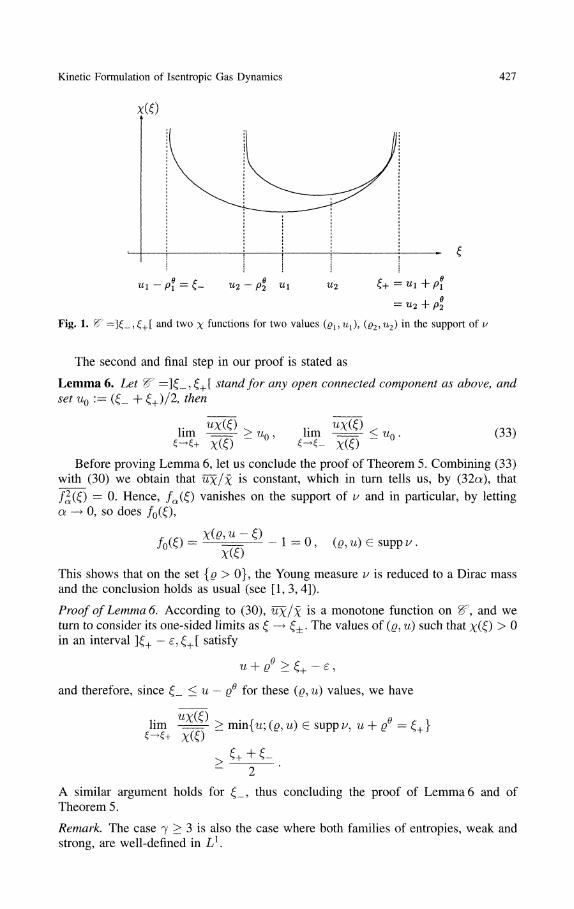
Fig. 1. ^ =]ξ_,£+[ and two χ functions for two values

= U2 + pi

(ρ2,u2) in the support of 1/

The second and final step in our proof is stated as

Lemma 6. Let W =]£_, ξ+[ stand for any open connected component as above, andset u0 := (ξ_ + ξ+)/2, then

lim lim (33)

Before proving Lemma 6, let us conclude the proof of Theorem 5. Combining (33)with (30) we obtain that ΰχ/χ is constant, which in turn tells us, by (32α), thatfa(0 = 0 Hence, fa(ξ) vanishes on the support of v and in particular, by lettinga —> 0, so does

This shows that on the set {ρ > 0}, the Young measure v is reduced to a Dirac massand the conclusion holds as usual (see [1, 3,4]).

Proof of Lemma 6. According to (30), ΰχ/χ is a monotone function on W, and weturn to consider its one-sided limits as ξ —> ξ±. The values of (ρ, u) such that χ(ξ) > 0in an interval ]ξ+ - ε, ξ+[ satisfy

u + ρθ > ξ+ - ε ,

and therefore, since ξ_ <u — ρθ for these (£>, n) values, we have

lim -=^ > min{^;(ρ,u) G suppv, u + ρθ = ξA

A similar argument holds for ξ_, thus concluding the proof of Lemma 6 and ofTheorem 5.

Remark. The case 7 > 3 is also the case where both families of entropies, weak andstrong, are well-defined in I,1.


III.2. The Case 7 = 3

In the case when 7 = 3, we have θ = 1 and the kinetic formulation reads

dtχ + ζdxχ = d^m. (34)

Thus, we can apply the averaging lemma in the version [5] and obtain

Proposition 7. Let (ρ, ρu) satisfy (1) with ρ°, ρ°(u0)2 + (ρ°)Ί in Lι(R), ρ° and u° inL°°(R), then

Q, Qu e Wζ£([0, +oo[xR) for all 0 < s < i (35)

where p = 1/4.

Remark. The regularity given by (35) is probably not optimal and is just an indicationof regularizing phenomena taking place in the case when 7 = 3.

Proof of Proposition 7. With these assumptions on the initial data we have

χ(t,x,ξ)eL°°(R+;L2(R2)),

m(ί, x, 0 G M 1 ^ x R2) (bounded measures),

and thus (35) follows from the general results of [5] observing that suppχ(ί,x, •) isuniformly bounded for x G 1R, t > 0.

IV. The p-System

To treat the case of Eq. (2), we follow the lines of Sects. I and II. We give first thekinetic formulation, then the invariant regions and finally the "dispersion" estimateanalogous to (3).

We only consider t?(£, x) > 0 and thus υ plays the role of ρ in the Eulerian case.

IV. 1. Kinetic Formulation

The couples entropy-entropy flux are now given by the relations

ηυυ+p'(v)ηww =0, (36)

Therefore the fundamental solutions to (36) are now

Yi(v; ξ — w) — υ(vι~Ί — (w — £ ) 2 ) i » λ = —r , (38)A 1 + 2(λ - 1)χ2(v, ξ-w) = (vι~Ί -{w- ξ)2)1, μ = -1 - λ . (39)

The entropy fluxes are obtained integrating g(ξ) against the function h given by

ζ — wh{(v,w;ξ) = θ Xι(V'9ξ-w), (40)

vv

h2(υ, w\ ξ) = θ ^ ^ χ2(v; ξ-w)+ I {sι~Ί - (ξ - w)2)^ ds. (41)

o


We still have θ — (7 — l)/2 and these formulae are obtained integrating the relationHυ = . . . in (37). Again, depending upon 7, these functions belong to L!(]R^) or notand in the following we restrict our attention to those cases corresponding to χλ £ L1,namely

1 < 7 < +00 . (42)

The energy is now given by

(43)2 7 — 1

It is always positive and its L ι norm in x decreases with t. Other entropies are givenby the

Lemma 8. η(υ, w) = f g(ξ)X\(v> ζ ~ w)dξ is a convex function ofv,w if and only ifg is convex. R

Proof of Lemma 8. Skipping standard calculations we have

_ 1 i,,-(7+D zυ θ)z(\ -z2)+dz

+ Jg"(...)z2(l-z2)λ

+dz

in 7 λ— / g (•••)(!" z )+ ^ > o ,

= ^ ^ ^ ~ ^ fg"{...)z{l-z2)ldz,

and we conclude again using Cauchy-Schwarz inequality and letting υ —» 0 or +00.As far as we are interested by shocks described by the convex entropies inw,υ, we

obtain that the entropy solutions to (2) with finite energy satisfy (recall that I7I > 1)

(44)

for some non-positive bounded measure m.

Remark. Notice that multiplying (44) by (ξ, ξ2/2) we recover the conservation of themomentum (second equation of (2)) and the energy inequality. The weight 1 does notgive the first conservation law, and we do not know how to recover the conservationlaw (associated of the conservation of mass) from (44).


TV.2. Invariant Regions

As before if χ{(t — 0,x,ξ) = 0 for ξ > ξ+, then this has to be true for all times(same for ξ < ξ_) thus recovering the maximum principle on the Riemann invariants

(w + v~θ) (x, t) < max(w° + (v°)~θ) (x), (45)X

(w - v'θ) (x, t) > mm(w° - (υ°)~θ) (x). (46)X

Thus v is bounded for 7 < — 1 and bounded from below for 7 > 1. In any case, wremains bounded.

IV. 3. An L£° Estimate of the Integral in Time

A straightforward application of (25) in Lemma 4 yields as in Sect. II the "dispersion"estimates

+00

I\\w\v1-^ +υ*¥1)(y,f)dt0

< C ί((w0)2 + (v°)ι~Ί)(x)dx , Vj/Gl, (47)

for entropy solutions with finite energy. Of course, for 7 > 1, those have infinite L1

norm of v but in that case the physical density is l/v.

Acknowledgements. The third author (E. Tadmor) has been partially supported by ONR ContractNr.N 00014-91 -J-1076 and DARPA Contract Nr. N0014-92-J-1890.

Note added in proof. After this work was achieved, other examples of kinetic formulation forN x N hyperbolic systems were obtained in [16].

References

1. Chen, G.Q.: The theory of compensated compactness and the System of Isentropic GasDynamics. Preprint MCS-P154-0590, University of Chicago, (1990)

2. Dafermos, CM.: Estimates for conservation laws with little viscosity. SIAM J. Math. Anal. 18,n. 2, 409-421 (1987)

3. DiPerna, R.J.: Convergence of Approximate Solutions to Conservation Laws. Arch. Rat. Mec.and Anal. 82(1), 27-70 (1983)

4. DiPerna, R.J.: Convergence of the Viscosity Method of Isentropic Gas Dynamics. Commun.Math. Phys. 91, 1-30 (1983)

5. DiPerna, R.J., Lions, P.L., Meyer, Y.: Lp Regularity of Velocity Averages. Ann. I.H.P. Anal.Non Lin. 8(3-4), 271-287 (1991)

6. Golse, F., Lions, P.L., Perthame, B., Sentis, R.: Regularity of the Moments of the Solution of aTransport Equation. J. Funct. Anal. 76, 110-125 (1988)

7. Lax, P.D.: Hyperbolic Systems of Conservation Laws and the Mathematical Theory of Shockwaves. CBMS-NSF regional conferences series in applied mathematics, 11 (1973)


8. Lions, P.L., Perthame, B.: Lemmes de moments, de moyenne et de dispersion. C.R. Acad. Sc.Paris, t. 314, serie I, 801-806 (1992)

9. Lions, P.L., Perthame, B., Tadmor, E.: Formulation cinetique des lois de conservation scalaires.C.R. Acad. Sci. Paris, t. 312, serie I, 97-102 (1991)

10. Lions, P.L., Perthame, B., Tadmor, E.: Kinetic Formulation of Scalar Conservation Laws.J.A.M.S. 7, 169-191 (1994)

11. Murat, F.: Compacite par compensation. Ann. Scuola Norm. Sup. Pisa 5, 489-507 (1978)12. Perthame, B.: Higher Moments Lemma: Applications to Vlasov-Poisson and Fokker-Planck

equations. Math. Meth. Appl. Sc. 13, 441-452 (1990)13. Serre, D.: Domaines invariants pour les systemes hyperboliques de lois de conservation. 69, n. 1,

46-62 (1987)14. Smoller, J.: Shock Waves and Reaction-Diffusion Equations. Berlin, Heidelberg, New York:

Springer 198215. Tartar, L.: Compensated Compactness and Applications to Partial Differential Equations. In:

Research Notes in Mathematics, Nonlinear analysis and mechanics, Heriot-Watt Symposium,Vol. 4, Knops, R.J. (ed.) London: Pitman Press, 1979

16. James, F., Peng, Y-J., Perthame, B.: Kinetic formulation for the chromatography and some otherhyperbolic systems (To appear in J. Math. Pures et Appl.)

Communicated by J. L. Lebowitz

Kinetic Formulation of the Isentropic Gas Dynamics …...Kinetic Formulation of the Isentropic Gas...

Documents

Transcript of Kinetic Formulation of the Isentropic Gas Dynamics …...Kinetic Formulation of the Isentropic Gas...