State the domain and range of each function. 3.1 Graphs of Exponential Functions.
JSS Journal of Statistical SoftwareJune 2017, Volume 78, Issue 10. doi: 10.18637/jss.v078.i10
KFAS: Exponential Family State Space Models in R
Jouni HelskeUniversity of Jyväskylä
Abstract
State space modeling is an efficient and flexible method for statistical inference of abroad class of time series and other data. This paper describes the R package KFAS forstate space modeling with the observations from an exponential family, namely Gaussian,Poisson, binomial, negative binomial and gamma distributions. After introducing thebasic theory behind Gaussian and non-Gaussian state space models, an illustrative exam-ple of Poisson time series forecasting is provided. Finally, a comparison to alternative Rpackages suitable for non-Gaussian time series modeling is presented.
Keywords: R, exponential family, state space models, time series, forecasting, dynamic linearmodels.
1. Introduction
State space models offer a unified framework for modeling several types of time series and otherdata. Structural time series, autoregressive integrated moving average (ARIMA) models,simple regression, generalized linear mixed models, and cubic spline smoothing are just someexamples of the statistical models which can be represented as a state space model. One ofthe simplest classes of state space models are linear Gaussian state space models (also knownas dynamic linear models), which are analytically tractable, and are therefore often used inmany fields of science.Petris and Petrone (2011) and Tusell (2011) introduce and review some of the contributed R(R Core Team 2017) packages available on the Comprehensive R Archive Network (CRAN)for Gaussian state space modeling. Since then, several new additions have emerged on CRAN.Most of these packages use one package or multiple packages reviewed in Tusell (2011) forfiltering and smoothing and add new user interfaces and functionality for certain types ofmodels. For example, package rucm (Chowdhury 2015) is focused on structural time series,dlmodeler (Szymanski 2014) provides a unified interface compatible with multiple packages,and MARSS (Holmes, Ward, and Wills 2012, 2013) provides functions for the maximum

2 KFAS: Exponential Family State Space Models in R
likelihood estimation of a large class of Gaussian state space models via the EM algorithm.One of the packages reviewed in the aforementioned papers is KFAS (for Kalman filteringand smoothing). Besides of modeling the general linear Gaussian state space models, KFAScan also be used in cases where the observations are from other exponential family models,namely binomial, Poisson, negative binomial, and Gamma models.After publication of the papers by Petris and Petrone (2011) and Tusell (2011), KFAS hasbeen completely rewritten. The package is now much more user-friendly due to the use ofR’s symbolic formulas in model definition. The non-Gaussian modeling, which was somewhatexperimental in the old versions of KFAS, is now fully functional supporting multivariatemodels with different distributions. Many other features have also been added (such as meth-ods for computing model residuals and predictions), the performance of the main functionshas improved and in the process several bugs have been fixed.In this paper we first introduce the basic theory related to state space modeling, and thenproceed to show the main aspects of KFAS in more detail, illustrate its functionality byapplying it to real life datasets, and finally make a short comparison between KFAS andother potentially useful packages for non-Gaussian time series modeling.
2. The Gaussian state space modelIn this section an introduction to key concepts regarding the theory of Gaussian state spacemodeling as in KFAS is given. As the algorithms behind KFAS are mostly based on Durbinand Koopman (2012) and the related articles by the same authors, the basic notation is nearlyidentical with the one used by them.For the linear Gaussian state space model with continuous states and discrete time intervalst = 1, . . . , n, we have
yt = Ztαt + εt, (observation equation)αt+1 = Ttαt +Rtηt, (state equation)
(1)
where εt ∼ N(0, Ht), ηt ∼ N(0, Qt) and α1 ∼ N(a1, P1) independently of each other. Weassume that yt is a p × 1, αt+1 is an m × 1 and ηt is a k × 1 vector. We also denoteα = (α>1 , . . . , α>n )> and similarly y = (y>1 , . . . , y>n )>.Here yt contains the observations at time t, whereas αt is a vector of the latent state processat time point t. The system matrices Zt, Tt, and Rt, together with the covariance matricesHt and Qt depend on the particular model definition, and are often time invariant, i.e.,do not depend on t. Usually at least some of these matrices contain unknown parameterswhich need to be estimated. In KFAS one defines the model with the function SSModel.The function SSModel only builds the model and does not perform estimation of unknownparameters, which differs from functions like lm, which builds and estimates the model withone command.The main goal of state space modeling is to gain knowledge of the latent states α given theobservations y. This is achieved by using two important recursive algorithms, the Kalmanfiltering and smoothing. From the Kalman filtering algorithm we obtain the one-step-aheadpredictions and the prediction errors
at+1 = E(αt+1|yt, . . . , y1),vt = yt − Ztat

Journal of Statistical Software 3
and the related covariance matrices
Pt+1 = VAR(αt+1|yt, . . . , y1),Ft = VAR(vt) = ZtPtZ
>t +Ht.
Using the results of the Kalman filtering, we establish the state smoothing equations runningbackwards in time and yielding
αt = E(αt|yn, . . . , y1),Vt = VAR(αt|yn, . . . , y1).
Similar smoothed estimates can also be computed for the disturbance terms εt and ηt, andstraightforwardly for the signal θt = Ztαt. For details on these algorithms, see Appendix Aand Durbin and Koopman (2012).A prior distribution of the initial state vector α1 can be defined as a multivariate Gaussiandistribution with mean a1 and covariance matrix P1. For an uninformative diffuse prior, onetypically sets P1 = κI, where κ is 107, for example. However, this method can be numericallyunstable due to cumulative roundoff errors. To solve this issue Koopman and Durbin (2003)present the exact diffuse initialization method, where the diffuse elements in a1 are set to zeroand P1 is decomposed as κP∞,1+P∗,1, where κ→∞. Here P∞,1 is a diagonal matrix with oneson those diagonal elements which relate to the diffuse elements of α1, and P∗,1 contains thecovariances of the nondiffuse elements of α1 (and zeros elsewhere). At the start of the Kalmanfiltering (and at the end of backward smoothing) we use so-called exact diffuse initializationformulas until P∞,t becomes a zero matrix, and then continue with the usual Kalman filteringequations. This exact method should be less prone to numerical errors, although they can stilloccur especially in the smoothing phase, if we, for example, have high collinearity betweenthe explanatory variables of the model. Note that given all the parameters in the systemmatrices, results from the Kalman filter and smoother are equivalent with Bayesian analysisgiven the same prior distribution for α1.When we have multivariate observations, it is possible that in the diffuse phase the matrixFt is not invertible, and the computation of at+1 and Pt+1 becomes impossible. On the otherhand, even if Ft is invertible, the computations can become slow when the dimensionalityof Ft, that is, the number of series increases. Also in the case of multivariate observations,the formulas relating to the diffuse initialization become cumbersome. Based on the ideas ofAnderson and Moore (1979), a complete univariate approach for filtering and smoothing wasintroduced by Koopman and Durbin (2000) (known as sequential processing by Anderson andMoore). The univariate approach is based on the alternative representation of the model (1),namely
yt,i = Zt,iαt,i + εt,i, i = 1, . . . , pt, t = 1, . . . , n,αt,i+1 = αt,i, i = 1, . . . , pt − 1,αt+1,1 = Ttαt,pt +Rtηt, t = 1, . . . , n,
and a1,1 ∼ N(a1, P1), with the assumption that Ht is diagonal for all t. Here the dimension ofthe observation vector yt can vary over time and therefore missing observations are handledstraightforwardly by adjusting the dimensionality of yt. In the case of non-diagonal Ht,the original model can be transformed either by taking the LDL decomposition of Ht, andmultiplying the observation equation with the L−1
t , so ε∗t ∼ N(0, Dt), or by augmenting the

4 KFAS: Exponential Family State Space Models in R
state vector with ε, when Qt becomes block diagonal with blocks Qt and Ht. Augmentingcan also be used for introducing a correlation between ε and η. Both the LDL decompositionand the state vector augmentation are supported in KFAS.In theory, when using the univariate approach, the computational costs of filtering andsmoothing decrease, as the number of matrix multiplications decrease, and there is no needfor solving the system of equations (Durbin and Koopman 2012, p. 159). As noted in Tusell(2011), these gains can somewhat cancel out as more calls to linear algebra functions areneeded and the memory management might not be as effective as working with larger objectsat once. Nevertheless, as noted previously, sequential processing has also other clear benefits,especially with diffuse initialization where the univariate approach simplifies the recursionsconsiderably (Durbin and Koopman 2012).KFAS uses this univariate approach in all cases. Although vt, Ft, and Kt = PtZ
>t =
COV(at, yt|yt−1, . . . , y1) differ from the standard multivariate versions, we get at = at,1 andPt = Pt,1 by using the univariate approach. If standard multivariate matrices Ft and Kt areneeded for inference, they can be computed later from the results of the univariate filter. Asthe covariances F∗,i,t, K∗,i,t, and P∗,t relating to the diffuse phase (see Appendix A) coincidewith the nondiffuse counterparts if F∞,i,t = 0, the asterisk is dropped from the variable namesin KFAS, and, for example, the variable F is an n× p array containing F∗,i,t and Fi,t, whereasFinf is an n× d array, where d is the last time point before the diffuse phase ended.
2.1. Log-likelihood of the Gaussian state space model
The Kalman filter equations can be used for computing the log-likelihood, which in its stan-dard form is
logL = −np2 log 2π − 12
n∑t=1
(log |Ft|+ v>t F−1t vt).
In the case of the univariate treatment and diffuse initialization, the diffuse log-likelihood canbe written as
logLd = −12
n∑t=1
pt∑i=1
wi,t,
where
wi,t ={
logF∞,i,t, if F∞,i,t > 0,I(Fi,t > 0)(log 2π + logFi,t + v2
i,tF−1i,t ), if F∞,i,t = 0,
see Durbin and Koopman (2012, Chapter 7) for details. Francke, Koopman, and De Vos (2010)show that there are cases where the above definition of diffuse log-likelihood is not optimal.Without going into the details, if system matrices Zt or Tt contain unknown parameters intheir diffuse parts, the diffuse likelihood is missing one term which depends on those unknownparameters. Francke et al. (2010, p. 411–412) present a recursive formula for computing thisextra term, which is also supported by KFAS.
2.2. Example of a Gaussian state space model
Now the theory of the previous sections is illustrated via an example. Our time series consistsof yearly alcohol-related deaths per 100,000 persons in Finland for the years 1969–2007 in theage group of 40–49 years (Figure 1). The data is taken from Statistics Finland (2014a,b).

Journal of Statistical Software 5
Year
Alc
ohol
−re
late
d de
aths
in F
inla
nd p
er 1
00,0
00 p
erso
ns
1970 1980 1990 2000
010
2030
4050
60
Figure 1: Alcohol-related deaths in Finland in the age group of 40–49 years (black line) withpredicted (red) and smoothed (blue) estimates.
For the observations y1, . . . , yn we assume that yt ∼ N(µt, σε) for all t = 1, . . . , n, where µt isa random walk with drift process
µt+1 = µt + ν + ηt
with ηt ∼ N(0, σ2η). Assume that we have no prior information about the initial state µ1 or
the constant slope ν. This model can be written in a state space form by defining
Z =(
1 0), H = σ2
ε , T =(
1 10 1
),
αt =(µtνt
), R =
(10
), Q = σ2
η,
a1 =(
00
), P∗,1 =
(0 00 0
), P∞,1 =
(1 00 1
).
In KFAS, this model can be written with the following code. For illustrative purposes wedefine all the system matrices manually without resorting to default values.
R> data("alcohol", package = "KFAS")R> deaths <- window(alcohol[, 2], end = 2007)R> population <- window(alcohol[, 6], end = 2007)R> Zt <- matrix(c(1, 0), 1, 2)R> Ht <- matrix(NA)R> Tt <- matrix(c(1, 0, 1, 1), 2, 2)

6 KFAS: Exponential Family State Space Models in R
R> Rt <- matrix(c(1, 0), 2, 1)R> Qt <- matrix(NA)R> a1 <- matrix(c(1, 0), 2, 1)R> P1 <- matrix(0, 2, 2)R> P1inf <- diag(2)R> model_gaussian <- SSModel(deaths / population ~ -1 ++ SSMcustom(Z = Zt, T = Tt, R = Rt, Q = Qt, a1 = a1, P1 = P1,+ P1inf = P1inf), H = Ht)
The first argument to the SSModel function is the formula which defines the observations (leftside of tilde operator ~) and the structure of the state equation (right side of tilde). Heredeaths / population is a univariate time series, and the state equation is defined usingthe system matrices with auxiliary function SSMcustom, and the intercept term is omittedwith -1 in order to keep the model identifiable. The observation level variance is defined viathe argument H. The NA values represent the unknown variance parameters σ2
ε and σ2η which
can be estimated using the function fitSSM. After estimation, the filtering and smoothingrecursions are performed using the KFS function.
R> fit_gaussian <- fitSSM(model_gaussian, inits = c(0, 0), method = "BFGS")R> out_gaussian <- KFS(fit_gaussian$model)
In this case, the maximum likelihood estimates are 9.5 for σ2ε and 4.3 for σ2
η.From the Kalman filter algorithm we get one-step-ahead predictions for the states at =(µt, νt)>. Note that even though the slope term ν was defined as time-invariant (νt = ν) inour model, it is recursively estimated by the Kalman filter. Thus at each time point t whenthe new observation yt becomes available, the estimate of ν is updated to take account of thenew information given by yt. At the end of Kalman filtering, an+1 gives our final estimate ofthe constant slope term given all of our data. Here the slope term is estimated as 0.84 withstandard error 0.34. For µt, the Kalman filter gives the one-step-ahead predictions, but asthe state is time-varying, we need to run also the smoothing algorithm if we are interested inthe estimates of µt for t = 1, . . . , n given all the data.Figure 1 shows the observations with one-step-ahead predictions (red) and smoothed (blue)estimates of the random walk process µt. Notice the typical pattern: At the time t theKalman filter computes the one-step-ahead prediction error vt = yt − µt, and uses this andthe previous prediction to correct the prediction for the next time point (see Appendix Afor the detailed update formula). Here this is most easily seen at the beginning of the serieswhere our predictions seem to be lagging the observations by one time step. On the otherhand, the smoothing algorithm takes account of both the past and the future values at eachtime point, thus producing more smoothed estimates of the latent process.
3. State space models for the exponential familyKFAS can also deal with observations which come from distributions of an exponential familyclass other than Gaussian. We assume that the state equation is as in the Gaussian case, butthe observation equation has the form
p(yt|θt) = p(yt|Ztαt),

Journal of Statistical Software 7
where θt = Ztαt is the signal and p(yt|θt) is the observational density.The signal θt is the linear predictor which is connected to the expected value E(yt) = µt viaa link function l(µt) = θt. In KFAS, the following distributions and links are available:
1. Gaussian distribution with mean µt and variance ut with identity link θt = µt.
2. Poisson distribution with intensity λt and exposure ut together with log-link θt =log(λt). Thus we have E(yt|θt) = VAR(yt|θt) = ute
θt .
3. Binomial distribution with size ut and probability of success πt. KFAS uses logit-linkso θt = logit(πt) resulting E(yt|θt) = utπt and VAR(yt|θt) = ut(πt(1− πt)).
4. Gamma distribution with a shape parameter ut and an expected value µt, again withlog-link θt = log(µ), where the Gamma distribution is defined as
p(yt|µt, ut) = uuttΓ(ut)
µ−utt yut−1t e
ytutµt .
This gives us E(yt|θt) = eθt and VAR(yt|θt) = e2θt/ut.
5. Negative binomial distribution with a dispersion parameter ut and an expected valueµt with log-link θt = log(µt), where the negative binomial distribution is defined as
p(yt|µt, ut) = Γ(yt + ut)Γ(ut)yt!
µytt uutt
(µt + ut)ut+yt,
giving us E(yt|θt) = eθt and VAR(yt|θt) = eθt + e2θt/ut.
Note that the variable ut has a different meaning depending on the distribution it is linkedto. In KFAS one defines the distribution for each time series via argument distribution andthe additional known parameters ut corresponding to each series as columns of the matrix u.In order to make inferences of the non-Gaussian models, we first find a Gaussian model whichhas the same conditional posterior mode as p(θ|y) (Durbin and Koopman 2000). This is doneusing an iterative process with Laplace approximation of p(θ|y), where the updated estimatesfor θt are computed via the Kalman filtering and smoothing from the approximating Gaussianmodel. In the approximating Gaussian model the observation equation is replaced by
yt = Ztαt + εt, εt ∼ N(0, Ht),
where the pseudo-observations yt variances Ht are based on the first and second derivativesof log p(yt|θt) with respect to θt (Durbin and Koopman 2000).Final estimates θt correspond to the mode of p(θ|y). In the Gaussian case the mode is alsothe mean. In cases listed in (1)–(5) the difference between the mode and the mean is oftennegligible. Nevertheless, we are usually more interested in µt than in the linear predictor θt.As the link function is non-linear, direct transformation µt = l−1(θt) introduces some bias. Tosolve this problem KFAS also contains methods based on importance sampling, which allowus to correct these possible approximation errors. With the importance sampling techniquewe can also compute the log-likelihood and the smoothed estimates for f(α), where f is anarbitrary function of states, exp(Ztαt) being a typical example.

8 KFAS: Exponential Family State Space Models in R
In the importance sampling scheme, we first find the approximating Gaussian model, simulatethe states αi from this Gaussian model and then compute the corresponding weights wi =p(y|αi)/g(y|αi), where p(y|αi) represents the conditional non-Gaussian density of the originalobservations, and g(y|αi) is the conditional Gaussian density of the pseudo-observations y.These weights are then used for computing
E(f(α)|y) =∑Ni=1 f(αi)wi∑N
i=1wi.
The simulation of Gaussian state space models in KFAS is based on the simulation smoothingalgorithm by Durbin and Koopman (2002). In order to improve simulation efficiency, KFAScan use two antithetic variables in the simulation algorithms. See Durbin and Koopman(2012, p. 265–266) for details on how these are constructed.KFAS also provides means for the filtering of non-Gaussian models. This is achieved by se-quentially using the smoothing scheme for (y1, . . . , yt), t = 1 . . . , n with yt set as missing. Thisis a relatively slow procedure for large models, as the importance sampling algorithms need tobe performed n times, although the first steps are much faster than the one using the wholedata. The non-Gaussian filtering is mainly for the computation of recursive residuals (seeSection 4) and for illustrative purposes, where computational efficiency is not that important.With large models or online-filtering problems, one is recommended to use a proper particlefilter approach, which is out of the scope of this paper.For non-Gaussian exponential family models in the context of generalized linear models, atypical way of obtaining the confidence interval of the prediction is to compute confidenceintervals in the scale of the linear predictor, and then the interval is transformed to the scaleof the observations. The issue of prediction intervals is often dismissed. For obtaining properprediction intervals in the case of non-Gaussian state space models, the following algorithmis used in KFAS.
(1) Draw N replicates of the linear predictor θ from the approximating Gaussian densityg(θ|y) with importance weights p(y|θ)/g(y|θ). Denote this sample θ1, . . . , θN as θ.
(2) Using the importance weights as sampling probabilities, draw a sample of size N withreplacement from θ. We now have N independent draws from p(θ|y).
(3) For each θi sampled in Step (2), take a random sample of yi from the observationaldistribution p(y|θi).
(4) Compute the the prediction intervals as empirical quantiles from y1, . . . , yN .
Assuming all the model parameters are known, these intervals coincide (within the MonteCarlo error) with the ones obtained from Bayesian analysis using the same priors for states.
3.1. Log-likelihood of the non-Gaussian state space modelThe log-likelihood function for the non-Gaussian model can be written as (Durbin and Koop-man 2012, p. 272)
logL(y) = log∫p(α, y)dα
= logLg(y) + log Eg[p(y|θ)g(y|θ)
],

Journal of Statistical Software 9
where Lg(y) is the log-likelihood of the Gaussian approximating model and the expectationis taken with respect to the Gaussian density g(α|y). The expectation can be approximatedby
log Eg[p(y|θ)g(y|θ)
]≈ log 1
N
N∑i=1
wi. (2)
In many cases, a good approximation of the log-likelihood can be computed without anysimulation, by setting N = 0 and using the mode estimate θ from the approximating model.In practice (2) suffers from the fact that wi = p(y|θi)/g(y|θi) is numerically unstable; whenthe number of observations is large, the discrete probability mass function p(y|θi) tends tozero, even when the Gaussian density function g(y|αi) does not. Therefore it is better toredefine the weights as
w∗i = p(y|θi)/p(y|θ)g(y|θi)/g(y|θ)
.
The log-likelihood is then computed as
log L(y) = logLg(y) + log w + log 1N
N∑i=1
w∗i ,
where w = p(y|θ)/g(y|θ).
3.2. Example of non-Gaussian state space model
The alcohol-related deaths of Section 2.2 can also be modeled naturally as a Poisson process.Now our observations yt are the actual counts of alcohol-related deaths in year t, whereas thevarying population size is taken into account by the exposure term ut. The state equationremains the same, but the observation equation is now of form p(yt|µt) = Poisson(uteµt).
R> model_poisson <- SSModel(deaths ~ -1 ++ SSMcustom(Z = Zt, T = Tt, R = Rt, Q = Qt, P1inf = P1inf),+ distribution = "poisson", u = population)
Compared to the Gaussian model of Section 2.2, we now need to define the distribution ofthe observations using the argument distribution (which defaults to "gaussian"). We alsodefine the exposure term via the argument u (for non-Gaussian models the H is omitted andvice versa), and use default values for a1 and P1 in the SSMcustom.In this model there is only one unknown parameter, σ2
η. This is estimated as 0.0053, but theactual values of σ2
η between the Gaussian and Poisson models are not directly comparableas the interpretation of µt differs between models. The slope term of the Poisson model isestimated as 0.022 with standard error 1.4× 10⁻⁴, corresponding to the 2.3% yearly increasein deaths.Figure 2 shows the smoothed estimates of the intensity (deaths per 100,000 persons) modeledas Gaussian process (blue), and as a Poisson process (red).

10 KFAS: Exponential Family State Space Models in R
Year
Alc
ohol
−re
late
d de
aths
in F
inla
nd p
er 1
00,0
00 p
erso
ns
1970 1980 1990 2000
2030
4050
60
Figure 2: Alcohol-related deaths in Finland (black line) with smoothed estimates from theGaussian model (blue) and the Poisson model (red).
4. ResidualsFor exponential family state space models, multiple types of residuals can be computed.Probably the most useful ones are standardized recursive residuals, which are based on theone-step-ahead predictions from the Kalman filter. For the univariate case these are definedas
yt − E(yt|yt−1, . . . , y1)√VAR(yt|yt−1, . . . , y1)
, t = d+ 1 . . . , n,
where d is the last time point of the diffuse phase, and the denominator can be decomposedas
VAR(yt|yt−1, . . . , y1) == VAR(E(yt|θt, yt−1, . . . , y1)|yt−1, . . . , y1) + E(VAR(yt|θt, yt−1, . . . , y1)|yt−1, . . . , y1)= VAR(E(yt|θt)|yt−1, . . . , y1) + E(VAR(yt|θt)|yt−1, . . . , y1).
In the Gaussian case this simplifies to vtF− 1
2t .
For multivariate observations we have several options on how to standardize the residuals.The most common one is a marginal standardization approach, where each residual seriesis divided by its standard deviation, so we get residual series which should not exhibit anyautocorrelations. Another option is to use, for example, Cholesky decomposition for theprediction error covariance matrix Ft and standardize the residuals by L−1
t (yt − yt) whereLtL
>t = Ft. Now the whole series of residuals (treated as a single univariate series) should
not contain any autocorrelation.

Journal of Statistical Software 11
For computing the marginally standardized residuals, multivariate versions of Ft and vt areneeded, whereas the Cholesky standardized residuals can be computed directly from thesequential Kalman filter as
vi,tF− 1
2it
, j = 1, . . . , p, t = d+ 1 . . . , n.
These multivariate residuals depend on the ordering of the series, so if the residual diagnosticsexhibit deviations from model assumptions, then the interpretation is somewhat more difficultthan when using the marginal residuals. Therefore marginal residuals might be preferred.Note that if we want quadratic form residuals (yt− yt)>F−1
t (yt− yt), then the ordering of theseries does not matter.The recursive residuals are defined just for the non-diffuse phase, which is problematic if themodel contains a long diffuse phase, for example, because a dummy variable with a diffuseprior is incorporated into the model. This is because the diffuse phase cannot end beforethe dummy variable changes its value at least once. In order to circumvent this, one canuse a proper but highly non-informative prior distribution for the intervention variable whencomputing the residuals, which should have a negligible effect on the visual inspection of theresidual plots.Other potentially useful residuals are auxiliary residuals, which are based on smoothed valuesof states. For details, see Harvey and Koopman (1992) and Durbin and Koopman (2012,Chapter 7).
5. Functionality of KFASThe state space model used with KFAS is built using the function SSModel. The function usesR’s formula object in a similar way to that of the functions lm and glm, for example. In orderto define the different components of the state space model, auxiliary functions SSMtrend,SSMseasonal, SSMcycle, SSMarima, SSMregression are provided. These functions can beused to define the structural, ARIMA, and regression components of the model. The functionSSMcustom can be used for constructing an arbitrary component by directly defining thesystem matrices of the model (1). More details on how to construct common state spacemodels with KFAS are presented in Section 6.The function SSModel returns an object of class ‘SSModel’, which contains the observations yas the ‘ts’ object, system matrices Z, H, T, R, Q as arrays of appropriate dimensions, togetherwith matrices a1, P1, and P1inf defining the initial state distribution. Additional componentscontain the system matrix u which is used in non-Gaussian models for additional parame-ters, the character vector distribution which defines the distributions of the observations(multivariate series can have different distributions), and the tolerance parameter tol whichis used in diffuse phase for checking whether F∞ is nonzero.The ‘SSModel’ object also contains some attributes, namely, integer valued attributes p, m, k,and n which define the dimensions of the system matrices, character vectors state_types andeta_types which define the elements of αt and ηt, and integer vector tv which defines whetherthe model contains time-varying system matrices. These attributes are used internally byKFAS, although the user can carefully modify them if needed. For example, if the userwishes to redefine the error term ηt by changing the dimensions of R and Q, the attributes kand eta_types need to be updated accordingly.

12 KFAS: Exponential Family State Space Models in R
The unknown model parameters can be estimated with fitSSM, which is a wrapper aroundR’s optim function and the logLik method for the ‘SSModel’ object. For fitSSM, the usergives the model object, initial values of unknown parameters and a function updatefn, whichis used to update the model given the parameters (the help page of fitSSM gives an exampleof updatefn). As the numerical optimization routines update the model and compute thelikelihood thousands of times, the user is encouraged to build their own problem-specificmodel updating function for maximum efficiency. By default, fitSSM estimates the NA valuesin the time invariant covariance matrices H and Q, but no general estimation function isprovided. Of course, the user can also directly use the logLik method for computing thelikelihood and thus is free to choose a suitable optimization method for their problem.The function KFS computes the filtered (one-step-ahead prediction) and smoothed estimatesfor states, signals, and the values of the inverse link function (expected value µ or probabilityπ) in a non-Gaussian case. For Gaussian models, disturbance smoothing is also available.With simulateSSM the user can simulate the states, signals or disturbances of the Gaussianstate space models given the model and the observations. If the model contains missingobservations, these can also be simulated by simulateSSM in a similar way. It is also possibleto simulate states from predictive distributions p(αt|y1, . . . , yt−1), t = 1, . . . , n. For thesesimulations, instead of using marginal distributions N(at, Pt), KFAS uses a modification ofDurbin and Koopman (2002), where smoothing is replaced by filtering.For non-Gaussian models, importanceSSM returns the states or signals simulated from theapproximating Gaussian model, and the corresponding weights wi, which can then be usedto compute arbitrary functions of the states or signals.There are several S3 methods available for ‘SSModel’ and ‘KFS’ objects. For both objectclasses, simple print methods are provided, and for ‘SSModel’ objects there is the logLikmethod. The predict method is for computing the point predictions together with confidenceor prediction intervals. The extraction operator [ for extracting and replacing the subsets ofmodel elements is available for the ‘SSModel’ class. Using this method when modifying themodel is suggested instead of a common list extractor $, as the latter can accidentally modifythe dimensions of the corresponding model matrices. A simple plot method for residualinspection is also provided.For the ‘KFS’ object, the methods residuals, rstandard, and hatvalues are provided. Also,a function signal can be used for extracting subsets of signals from ‘KFS’ objects, for example,the part of Ztαt that corresponds to the regression part of the model.Methods coef and fitted for the quick extraction of state or mean estimates are also availablefor ‘KFS’ and ‘SSModel’ objects.
6. Constructing common state space models with KFASThis section presents some typical models which can be formulated in a state space form. Moreexamples can be found on the main help page of KFAS by typing ?KFAS after the packageis loaded via library("KFAS"). These examples include most of the examples presented inDurbin and Koopman (2012). Additional examples illustrating the functionality of KFAS canbe found from the documentation of the particular functions.All the auxiliary functions used in the formula argument of the function SSModel have somecommon arguments which are not directly related to the system matrices of the corresponding

Journal of Statistical Software 13
component. In complex multivariate models, an important argument is index, which definesthe series for which the corresponding component is constructed. For example, if we havefour time series (p = 4), we may want to use a certain regression component only for series2 and 4. In this case we use the argument index = c(2, 4) when calling the appropriateSSMregression function. By default the index is 1:p so the component is constructed for allseries.Another argument used in several auxiliary functions is type, which can take two possiblevalues. The value "distinct" defines the component separately for each series defined byindex (with covariance structure defined by the argument Q), whereas the value "common"constructs a single component which applies to all series defined by index. For example, wecan define distinct random walk components for all series together with a covariance matrixwhich captures the dependencies of the different series, or we can define just a single randomwalk component which is common to all series.
6.1. Structural time series
A structural time series refers to the class of state space models where the observed timeseries is decomposed into several underlying components, such as trend and seasonal effects.The basic structural time series model is of the form
yt = µt + γt + ct + εt, εt ∼ N(0, Ht),µt+1 = µt + νt + ξt, ξt ∼ N(0, Qlevel,t),νt+1 = νt + ζt, ζt ∼ N(0, Qslope,t),
(3)
where µt is the trend component, γt is the seasonal component and ct is the cycle component.The seasonal component with period s can be defined in a dummy variable form
γt+1 = −s−1∑j=1
γt+1−j + ωt, ωt ∼ N(0, Qseasonal,t),
or in a trigonometric form, where
γt =bs/2c∑j=1
γj,t,
γj,t+1 = γj,t cosλj + γ∗j,t sinλj + ωj,t,
γ∗j,t+1 = −γj,t sinλj + γ∗j,t cosλj + ω∗j,t, j = 1, . . . , bs/2c,
with ωj,t and ω∗j,t being independently distributed variables with N(0, Qseasonal,t) distributionand λj = 2πj/s.The cycle component with period s is defined as
ct+1 = ct cosλc + c∗t sinλc + ωt,
c∗t+1 = −ct sinλc + c∗t cosλc + ω∗t ,
with ωt and ω∗t being independent variables from N(0, Qcycle,t) distribution and frequencyλc = 2π/s.

14 KFAS: Exponential Family State Space Models in R
For non-Gaussian models the observation equation of (3) is replaced by p(yt|θt), where θt =µt + γt + ct. An additional Gaussian noise term εt can also be included in θt using theSSMcustom function (which is illustrated in Section 6.5). The general matrix formulation ofstructural time series can be found, for example, in Durbin and Koopman (2012, Chapter 3).Three auxiliary functions, SSMtrend, SSMcycle, and SSMseasonal, for building structuraltime series are provided in KFAS. The argument degree of SSMtrend defines the degree ofthe polynomial component, where 1 corresponds to a local level model and 2 to a local lineartrend model. Higher order polynomials can also be defined with larger values. Anotherimportant argument for SSMtrend is Q, which defines the covariance structure of the trendcomponent. This is typically a list of p × p matrices (with p being the number of series forwhich the component is defined), where the first matrix corresponds to the level component(µ in (3)), the second to the slope component ν and so forth.The function SSMcycle differs from SSMtrend only by one argument. SSMcycle does not haveargument degree, but instead it has argument period which defines the length of the cyclect. The same argument is also used in the function SSMseasonal, which contains also anotherimportant argument sea.type, which can be used to define whether the user wants a dummyor a trigonometric seasonal.The example models of Sections 2.2 and 3.2 are special cases of the local linear trend model,where the variance of ζt is zero, and there are no seasonal or cycle components. Thus theGaussian model of Section 2.2 can be built with KFAS more easily by the following code:
R> model_structural <- SSModel(deaths / population ~+ SSMtrend(degree = 2, Q = list(matrix(NA), matrix(0))), H = matrix(NA))R> fit_structural <- fitSSM(model_structural, inits = c(0, 0),+ method = "BFGS")R> fit_structural$model["Q"]
, , 1
[,1] [,2][1,] 4.256967 0[2,] 0.000000 0
Here the state equation is defined using the SSMtrend auxiliary function without the need foran explicit definition of the corresponding system matrices. The intercept term is automat-ically omitted from the right side of the formula when the SSMtrend component is used, inorder to keep the model identifiable. Here the unknown variance parameters are set to NA, sothe default behavior of the fitSSM function can be used for the parameter estimation.
6.2. ARIMA models
Another typical time series modeling framework are ARIMA models, which are also possibleto define as a state space model. The auxiliary function SSMarima defines the ARIMA modelusing vectors ar and ma, which define the autoregressive and moving average coefficients,respectively. The function assumes that all series defined by the index have the same coeffi-cients. The argument d defines the degree of differencing, and a logical argument stationary

Journal of Statistical Software 15
defines whether stationarity (after differencing) is assumed (if not, diffuse initial states areused instead of a stationary distribution). A univariate ARIMA(p, d, q) model can be writtenas
y∗t = φ1y∗t−1 + . . .+ φpy
∗t−p + ξt + θ1ξt−1 + . . .+ θqξt−q,
where y∗t = ∆dyt and ξt ∼ N(0, σ2). Let r = max(p, q + 1). KFAS defines the state spacerepresentation of the ARIMA(p, d, q) model with stationary initial distribution as
Z> =
1d+1
0...0
, H = 0, T =
Ud 1>d 0 · · · 00 φ1 1 0... . . .... φr−1 0 10 φr 0 · · · 0
, R =
0d1θ1...
θr−1
,
αt =
yt−1...
∆d−1yt−1y∗t
φ2y∗t−1 + . . .+ φry
∗t−r+1 + θ1ηt + . . .+ θr−1ηt−r+2
...φry∗t−1 + θr−1ηt
, Q = σ2,
a1 =
0...0
, P∗,1 =(
0 00 Sr
), P∞,1 =
(Id 00 0
), ηt = ξt+1,
where φp+1 = . . . = φr = θq+1 = . . . = θr−1 = 0, 1d+1 is a 1× (d+ 1) vector of ones, Ud is ad× d upper triangular matrix of ones and Sr is the covariance matrix of stationary elementsof α1. The elements of the initial state vector α1 which correspond to the differenced valuesy0, . . . ,∆d−1y0 are treated as diffuse. The covariance matrix Sr can be computed by solvingthe linear equation (I − T ⊗ T )vec(Sr) = vec(RR>) (Durbin and Koopman 2012, p. 138).Note that the arima function from package stats (R Core Team 2017) also uses the same statespace approach for ARIMA modeling, although the handling of the intercept and possiblecovariates is done in a slightly different manner (see documentation of arima for details).As an example, we again model the alcohol-related deaths but now use the ARIMA(0, 1, 1)model with drift:
R> drift <- 1:length(deaths)R> model_arima <- SSModel(deaths / population ~ drift ++ SSMarima(ma = 0, d = 1, Q = 1))R> update_model <- function(pars, model) {+ tmp <- SSMarima(ma = pars[1], d = 1, Q = pars[2])+ model["R", states = "arima"] <- tmp$R+ model["Q", states = "arima"] <- tmp$Q

16 KFAS: Exponential Family State Space Models in R
+ model["P1", states = "arima"] <- tmp$P1+ model+ }R> fit_arima <- fitSSM(model_arima, inits = c(0, 1), updatefn = update_model,+ method = "L-BFGS-B", lower = c(-1, 0), upper = c(1, 100))R> fit_arima$optim.out$par
[1] -0.4994891 16.9937888
In this case we need to supply the model updating function for fitSSM which updates ourmodel definition based on the current values of the parameters we are estimating. Instead ofmanually altering the corresponding elements of the model, update_model uses the SSMarimafunction for computation of relevant system matrices R,Q and P1. The estimated values forθ1 and σ are −0.5 and 17.Comparing the results of our previous structural time series model and the estimated ARIMAmodel, we see that the estimated drift term and the log-likelihood are identical:
R> (out_arima <- KFS(fit_arima$model))
Smoothed values of states and standard errors at time n = 39:Estimate Std. Error
drift 0.8409 0.3446arima1 20.3008 13.1100arima2 1.3545 1.3898arima3 0.3031 0.6453
R> (out_structural <- KFS(fit_structural$model))
Smoothed values of states and standard errors at time n = 39:Estimate Std. Error
level 54.7532 2.1705slope 0.8409 0.3446
R> out_arima$logLik
[1] -108.9734
R> out_structural$logLik
[1] -108.9734
This is not surprising given the well-known connections between structural time series andARIMA models (Harvey 1989).
6.3. Linear and generalized linear modelsAn ordinary linear regression model
yt = x>t β + εt, t = 1, . . . , n,
Journal of Statistical Software 17
where εt ∼ N(0, σ2), can be written as a Gaussian state space model by defining Zt = x>t ,Ht = σ2, Rt = Qt = 0 and αt = β. Assuming that the prior distribution of β is defined asdiffuse, the diffuse likelihood of this state space model corresponds to a restricted maximumlikelihood (REML). Then the estimate for σ2 obtained from fitSSM would be the familiarunbiased REML estimate of residual variance. It is important to notice that for this simplemodel numerical optimization is not needed, since we can estimate σ2 by running the Kalmanfilter with Ht = 1, which gives us
σ2 = 1∑I(F∞,t = 0)
n∑t=1
I(F∞,t = 0)v2t /Ft,
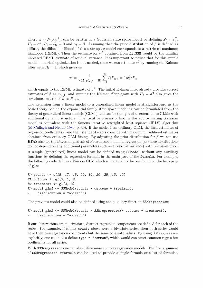
which equals to the REML estimate of σ2. The initial Kalman filter already provides correctestimates of β as an+1, and running the Kalman filter again with Ht = σ2 also gives thecovariance matrix of β as Pn+1.The extension from a linear model to a generalized linear model is straightforward as thebasic theory behind the exponential family state space modeling can be formulated from thetheory of generalized linear models (GLMs) and can be thought of as extension to GLMs withadditional dynamic structure. The iterative process of finding the approximating Gaussianmodel is equivalent with the famous iterative reweighted least squares (IRLS) algorithm(McCullagh and Nelder 1989, p. 40). If the model is an ordinary GLM, the final estimates ofregression coefficients β and their standard errors coincide with maximum likelihood estimatesobtained from ordinary GLM fitting. By adjusting the prior distribution for β we can useKFAS also for the Bayesian analysis of Poisson and binomial regression (as those distributionsdo not depend on any additional parameters such as a residual variance) with Gaussian prior.A simple (generalized) linear model can be defined using SSModel without any auxiliaryfunctions by defining the regression formula in the main part of the formula. For example,the following code defines a Poisson GLM which is identical to the one found on the help pageof glm:
R> counts <- c(18, 17, 15, 20, 10, 20, 25, 13, 12)R> outcome <- gl(3, 1, 9)R> treatment <- gl(3, 3)R> model_glm1 <- SSModel(counts ~ outcome + treatment,+ distribution = "poisson")
The previous model could also be defined using the auxiliary function SSMregression:
R> model_glm2 <- SSModel(counts ~ SSMregression(~ outcome + treatment),+ distribution = "poisson")
If our observations are multivariate, distinct regression components are defined for each of theseries. For example, if counts counts above were a bivariate series, then both series wouldhave their own regression coefficients but the same covariate values. By using SSMregressionexplicitly, one could also define type = "common", which would construct common regressioncoefficients for all series.With SSMregression one can also define more complex regression models. The first argumentof SSMregression, rformula can be used to provide a single formula or a list of formulas,
18 KFAS: Exponential Family State Space Models in R
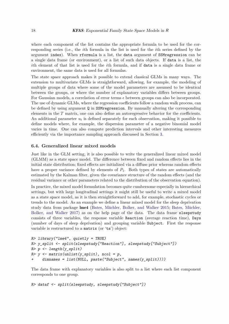
where each component of the list contains the appropriate formula to be used for the cor-responding series (i.e., the ith formula in the list is used for the ith series defined by theargument index). When rformula is a list, the data argument of SSMregression can bea single data frame (or environment), or a list of such data objects. If data is a list, theith element of that list is used for the ith formula, and if data is a single data frame orenvironment, the same data is used for all formulas.The state space approach makes it possible to extend classical GLMs in many ways. Theextension to multivariate GLMs is straightforward, allowing, for example, the modeling ofmultiple groups of data where some of the model parameters are assumed to be identicalbetween the groups, or where the number of explanatory variables differs between groups.For Gaussian models, a correlation of error terms ε between groups can also be incorporated.The use of dynamic GLMs, where the regression coefficients follow a random walk process, canbe defined by using argument Q in SSMregression. By manually altering the correspondingelements in the T matrix, one can also define an autoregressive behavior for the coefficients.An additional parameter ut is defined separately for each observation, making it possible todefine models where, for example, the dispersion parameter of a negative binomial modelvaries in time. One can also compute prediction intervals and other interesting measuresefficiently via the importance sampling approach discussed in Section 3.
6.4. Generalized linear mixed models
Just like in the GLM setting, it is also possible to write the generalized linear mixed model(GLMM) as a state space model. The difference between fixed and random effects lies in theinitial state distribution; fixed effects are initialized via a diffuse prior whereas random effectshave a proper variance defined by elements of P1. Both types of states are automaticallyestimated by the Kalman filter, given the covariance structure of the random effects (and theresidual variance or other parameters related to the distribution of the observation equation).In practice, the mixed model formulation becomes quite cumbersome especially in hierarchicalsettings, but with large longitudinal settings it might still be useful to write a mixed modelas a state space model, as it is then straightforward to add, for example, stochastic cycles ortrends to the model. As an example we define a linear mixed model for the sleep deprivationstudy data from package lme4 (Bates, Mächler, Bolker, and Walker 2015; Bates, Mächler,Bolker, and Walker 2017) as on the help page of the data. The data frame sleepstudyconsists of three variables, the response variable Reaction (average reaction time), Days(number of days of sleep deprivation) and grouping variable Subject. First the responsevariable is restructured to a matrix (or ‘ts’) object:
R> library("lme4", quietly = TRUE)R> y_split <- split(sleepstudy["Reaction"], sleepstudy["Subject"])R> p <- length(y_split)R> y <- matrix(unlist(y_split), ncol = p,+ dimnames = list(NULL, paste("Subject", names(y_split))))
The data frame with explanatory variables is also split to a list where each list componentcorresponds to one group.
R> dataf <- split(sleepstudy, sleepstudy["Subject"])

Journal of Statistical Software 19
The only explanatory variable Days in the data is identical to each subject so the previoussplit of the data frame is not necessary, but illustrates the workflow for more complex data.We can now build the state space model by defining the common fixed part for each group(SSMregression function with argument type = "common"). Using the same function wecan define the distinct random effect parts for each group, and the covariance structure of therandom effects using the argument P1 (the diffuse part P1inf is automatically set to zero forthose states where the corresponding element in P1 is nonzero). The function .bdiag fromthe Matrix package (Bates and Mächler 2017) is used for building a block diagonal covariancematrix for the random effects.
R> P1 <- as.matrix(.bdiag(replicate(p, matrix(NA, 2, 2), simplify = FALSE)))R> model_lmm <- SSModel(y ~ -1 ++ SSMregression(rep(list(~ Days), p), type = "common", data = dataf,+ remove.intercept = FALSE) ++ SSMregression(rep(list(~ Days), p), data = dataf,+ remove.intercept = FALSE, P1 = P1), H = diag(NA, p))
Note that in SSMregression, we use a list of formulas (the first unnamed argument rformula)and data frames (argument data), where each component corresponds to one column of y.Thus we could use different formulas for different groups in more complex models. In thissimple example the same model could be built with call
R> model_lmm2 <- SSModel(y ~ - 1 ++ SSMregression(~ Days, type = "common", remove.intercept = FALSE) ++ SSMregression(~ Days, remove.intercept = FALSE, P1 = P1),+ H = diag(NA, p), data = data.frame(Days = 0:9))
Again we need to define the model updating function for fitSSM:
R> update_lmm <- function(pars, model) {+ P1 <- diag(exp(pars[1:2]))+ P1[1, 2] <- pars[3]+ P1 <- crossprod(P1)+ model["P1", states = 3:38] <-+ as.matrix(.bdiag(replicate(p, P1, simplify = FALSE)))+ model["H"] <- diag(exp(pars[4]), p)+ model+ }R> fit_lmm <- fitSSM(model_lmm, c(1, 1, 1, 5), update_lmm, method = "BFGS")
The estimated likelihood, variance/covariance parameters, and the estimates of fixed andrandom effects are practically identical to the ones obtained by the lmer function of the lme4package. The only major difference is in the estimation of conditional covariance matricesof the random effects, which is due to the fact that in lme4 these matrices are computedconditionally on all the other model parameters, including the fixed effects (Bates et al. 2015,p. 28). In KFAS the conditioning is only on the numerically estimated variance/covarianceparameters, and thus the resulting standard errors of random effects also take into accountthe uncertainty of the estimation of fixed effects.

20 KFAS: Exponential Family State Space Models in R
In this example different groups were thought of as separate response vectors. In cases wherethe sample sizes in different groups are not equal, the same approach can be used afterappropriately filling the data matrix with missing values. The corresponding NA values incovariates do not cause problems as they are not referenced in the Kalman filter.It is also possible to define the mixed model using univariate response and time-varying systemmatrices Tt and Qt. This reduces the state space and thus makes the model computationallymore efficient, but adding other stochastic components to the model can be more problematic.For building such a model we need to use either the customSSM function for defining thecorresponding time-varying system matrices, or we can use SSMregression as a startingpoint and alter the model components manually. This univariate approach is illustrated onthe main help page of KFAS.
6.5. Arbitrary state space models
By combining the auxiliary functions presented in the previous sections and possibly man-ually adjusting the resulting system matrices, a large amount of models can be constructedwith relative ease. For cases where this is not sufficient or otherwise preferable, the auxiliaryfunction SSMcustom can be used for the construction of arbitrary components by direct defi-nition of the system matrices. As an example, we modify the Poisson model of Section 3 byadding an additional white noise term which tries to capture possible overdispersion of thedata. Our model for the Poisson intensity is now ut exp(µt + εt) with
µt+1 = µt + ν + ηt,
where ηt ∼ N(0, σ2η) as before, and εt ∼ N(0, σ2
ε ). This model can be written in a state spaceform by defining
R> model_poisson <- SSModel(deaths ~ SSMtrend(2, Q = list(NA, 0)) ++ SSMcustom(Z = 1, T = 0, Q = NA, P1 = NA), distribution = "poisson",+ u = population)
As the model contains unknown parameters in P1, we need to provide a specific model up-dating function for fitSSM:
R> update_poisson <- function(pars, model) {+ model["Q", etas = "level"] <- exp(pars[1])+ model["Q", etas = "custom"] <- exp(pars[2])+ model["P1", states = "custom"] <- exp(pars[2])+ model+ }R> fit_poisson <- fitSSM(model_poisson, c(-3, -3), update_poisson,+ method = "BFGS")R> fit_poisson$model["Q", etas = "level"]
[1] 0.00316852
R> fit_poisson$model["Q", etas = "custom"]

Journal of Statistical Software 21
Year
Alc
ohol
−re
late
d de
aths
in F
inla
nd p
er 1
00,0
00 p
erso
ns
1970 1980 1990 2000
2030
4050
60
Figure 3: Alcohol-related deaths in Finland (black line) with smoothed estimates from theGaussian model (blue) and the Poisson model with additional noise (red).
[1] 0.002506342
From Figure 3 we see that the Gaussian structural time series model and the Poisson structuraltime series model with additional white noise produce nearly indistinguishable estimates ofthe smoothed trend µt. This is due to the relatively high intensity of the Poisson process.
7. IllustrationWe now illustrate the use of KFAS with a more complete example case than the previousexamples. Again the data consists of alcohol-related deaths in Finland, but now four agegroups, 30–39, 40–49, 50–59 and 60–69, are modeled together as a multivariate Poisson model.The death counts and yearly population sizes in corresponding age groups are available for theyears 1969–2012, but as an illustration, we only use the data until 2007, and make predictionsfor the years 2008–2013. Figure 4 shows the number of deaths per 100,000 persons for all agegroups.
R> data("alcohol", package = "KFAS")R> colnames(alcohol)
[1] "death at age 30-39" "death at age 40-49"[3] "death at age 50-59" "death at age 60-69"[5] "population by age 30-39" "population by age 40-49"[7] "population by age 50-59" "population by age 60-69"

22 KFAS: Exponential Family State Space Models in R
Year
Alc
ohol
−re
late
d de
aths
in F
inla
nd p
er 1
00,0
00 p
erso
ns
1970 1980 1990 2000
2040
6080
100
death at age 30−39death at age 40−49death at age 50−59death at age 60−69
Figure 4: Alcohol-related deaths per 100,000 persons in Finland in 1969–2007 for four agegroups.
R> ts.plot(window(alcohol[, 1:4] / alcohol[, 5:8], end = 2007), col = 1:4,+ ylab = "Alcohol-related deaths in Finland per 100,000 persons",+ xlab = "Year")R> legend("topleft",col = 1:4, lty = 1, legend = colnames(alcohol)[1:4])
Here we choose a multivariate extension of the Poisson model used in Section 6.5:
p(yt|θt) = Poisson(uteθt), ut = populationt,θt = µt + εt, εt ∼ N(0, Qnoise),
µt+1 = µt + νt + ξt, ξt ∼ N(0, Qlevel),νt+1 = νt.
(4)
Here µt is the random walk with drift component, νt is a constant slope and εt is an addi-tional white noise component which captures the extra variation of the series. We make norestrictions for the covariance structures of the level or the noise component.The model (4) can be constructed with KFAS as follows.
R> alcoholPred <- window(alcohol, start = 1969, end = 2007)R> model <- SSModel(alcoholPred[, 1:4] ~+ SSMtrend(2, Q = list(matrix(NA, 4, 4), matrix(0, 4, 4))) ++ SSMcustom(Z = diag(1, 4), T = diag(0, 4), Q = matrix(NA, 4, 4),+ P1 = matrix(NA, 4, 4)), distribution = "poisson",+ u = alcoholPred[, 5:8])
The updating function for fitSSM is
Journal of Statistical Software 23
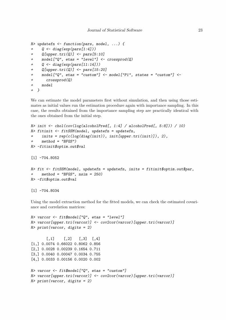
R> updatefn <- function(pars, model, ...) {+ Q <- diag(exp(pars[1:4]))+ Q[upper.tri(Q)] <- pars[5:10]+ model["Q", etas = "level"] <- crossprod(Q)+ Q <- diag(exp(pars[11:14]))+ Q[upper.tri(Q)] <- pars[15:20]+ model["Q", etas = "custom"] <- model["P1", states = "custom"] <-+ crossprod(Q)+ model+ }
We can estimate the model parameters first without simulation, and then using those esti-mates as initial values run the estimation procedure again with importance sampling. In thiscase, the results obtained from the importance sampling step are practically identical withthe ones obtained from the initial step.
R> init <- chol(cov(log(alcoholPred[, 1:4] / alcoholPred[, 5:8])) / 10)R> fitinit <- fitSSM(model, updatefn = updatefn,+ inits = rep(c(log(diag(init)), init[upper.tri(init)]), 2),+ method = "BFGS")R> -fitinit$optim.out$val
[1] -704.8052
R> fit <- fitSSM(model, updatefn = updatefn, inits = fitinit$optim.out$par,+ method = "BFGS", nsim = 250)R> -fit$optim.out$val
[1] -704.8034
Using the model extraction method for the fitted models, we can check the estimated covari-ance and correlation matrices:
R> varcor <- fit$model["Q", etas = "level"]R> varcor[upper.tri(varcor)] <- cov2cor(varcor)[upper.tri(varcor)]R> print(varcor, digits = 2)
[,1] [,2] [,3] [,4][1,] 0.0074 0.66022 0.8062 0.856[2,] 0.0028 0.00239 0.1654 0.711[3,] 0.0040 0.00047 0.0034 0.755[4,] 0.0033 0.00156 0.0020 0.002
R> varcor <- fit$model["Q", etas = "custom"]R> varcor[upper.tri(varcor)] <- cov2cor(varcor)[upper.tri(varcor)]R> print(varcor, digits = 2)

24 KFAS: Exponential Family State Space Models in R
[,1] [,2] [,3] [,4][1,] 0.00537 0.73118 0.75627 8.0e-01[2,] 0.00315 0.00346 0.99924 9.9e-01[3,] 0.00295 0.00313 0.00283 1.0e+00[4,] 0.00043 0.00043 0.00039 5.4e-05
Parameter estimation of a state space model is often a difficult task, as the likelihood surfacecontains multiple maxima, thus making the optimization problem highly dependent on theinitial values. Often the unknown parameters are related to the unobserved latent states,such as the covariance matrix in this example, with little a priori knowledge. Therefore, it ischallenging to guess good initial values, especially in more complex settings. Thus, the useof multiple initial value configurations possibly with several different types of optimizationroutines is recommended before one can be reasonably sure that the proper optimum is found.Here we use the covariance matrix of the observed series as initial values for the covariancestructures.Another issue in the case of non-Gaussian models is the fact that the likelihood computationis based on an iterative procedure which is stopped using some stopping criterion (such asthe relative change of log-likelihood), so the log-likelihood function actually contains somenoise. This in turn can affect the gradient computations in methods like BFGS and can intheory give unreliable results. Using a derivative free method like Nelder-Mead is thereforesometimes recommended. On the other hand, BFGS is usually much faster than Nelder-Mead,and thus we prefer to try BFGS first at least in preliminary analysis.Using the function KFS we can compute the smoothed estimates of states:
R> out <- KFS(fit$model, nsim = 1000)R> out
Smoothed values of states and standard errors at time n = 39:Estimate Std. Error
level.death at age 30-39 2.8559160 0.0784371slope.death at age 30-39 0.0107142 0.0137135level.death at age 40-49 4.0313117 0.0423763slope.death at age 40-49 0.0237188 0.0076318level.death at age 50-59 4.7578026 0.0398295slope.death at age 50-59 0.0503715 0.0095850level.death at age 60-69 4.4938371 0.0332897slope.death at age 60-69 0.0482386 0.0072090custom1 -0.0004021 0.0603946custom2 -0.0195488 0.0408846custom3 -0.0169493 0.0370236custom4 -0.0021345 0.0051427
From the output of KFS we see that the slope term is not significant in the first age group. Fortime-varying states we can easily plot the estimated level and noise components, which showsclear trends in three age groups and highly correlated additional variation in all groups:
R> plot(coef(out, states = c("level", "custom")), main = "Smoothed states",+ yax.flip = TRUE)

Journal of Statistical Software 25
2.4
2.6
2.8
3.0
leve
l.dea
th a
t age
30−
39
3.2
3.4
3.6
3.8
4.0
leve
l.dea
th a
t age
40−
49
3.0
3.5
4.0
4.5
leve
l.dea
th a
t age
50−
59
3.0
3.5
4.0
4.5
1970 1980 1990 2000 leve
l.dea
th a
t age
60−
69
Time
−0.
100.
00
cust
om1
−0.
100.
00
cust
om2
−0.
100.
000.
05
cust
om3
−0.
015
−0.
005
0.00
5
1970 1980 1990 2000
cust
om4
Time
Smoothed states
Figure 5: Smoothed level and white noise components.
Note the large drop in the noise component in Figure 5, which relates to a possible outlierin 1973 of the mortality series. As an illustration of model diagnostics, we compute recur-sive residuals for our model and check whether there is autocorrelation left in the residuals(Figure 6).
R> res <- rstandard(KFS(fit$model, filtering = "mean", smoothing = "none",+ nsim = 1000))R> acf(res, na.action = na.pass)
We see occasional lagged cross-correlation between the residuals, but overall we can be rela-tively satisfied with our model.We can now predict the intensity eθt of alcohol-related deaths per 100,000 persons for eachage group for years 2008–2013 using our estimated model. As our model is time varying (i.e.,u varies), we need to provide the model for the future observations via the newdata argument.In this case we can use the SSMcustom function and provide all the necessary system matricesat once, together with constant u = 1 (our signal θ is already scaled properly as the originalut was the population per 100,000 persons).

26 KFAS: Exponential Family State Space Models in R
0 2 4 6 8
−0.
40.
20.
61.
0
Lag
AC
F
death at age 30−39
0 2 4 6 8−
0.4
0.2
0.6
1.0
Lag
daa3 & daa4
0 2 4 6 8
−0.
40.
20.
61.
0
Lag
daa3 & daa5
0 2 4 6 8
−0.
40.
20.
61.
0
Lag
daa3 & daa6
−8 −6 −4 −2 0
−0.
40.
20.
61.
0
Lag
AC
F
daa4 & daa3
0 2 4 6 8
−0.
40.
20.
61.
0
Lag
death at age 40−49
0 2 4 6 8−
0.4
0.2
0.6
1.0
Lag
daa4 & daa5
0 2 4 6 8
−0.
40.
20.
61.
0
Lag
daa4 & daa6
−8 −6 −4 −2 0
−0.
40.
20.
61.
0
Lag
AC
F
daa5 & daa3
−8 −6 −4 −2 0
−0.
40.
20.
61.
0
Lag
daa5 & daa4
0 2 4 6 8
−0.
40.
20.
61.
0
Lag
death at age 50−59
0 2 4 6 8−
0.4
0.2
0.6
1.0
Lag
daa5 & daa6
−8 −6 −4 −2 0
−0.
40.
20.
61.
0
Lag
AC
F
daa6 & daa3
−8 −6 −4 −2 0
−0.
40.
20.
61.
0
Lag
daa6 & daa4
−8 −6 −4 −2 0
−0.
40.
20.
61.
0
Lag
daa6 & daa5
0 2 4 6 8
−0.
40.
20.
61.
0
Lag
death at age 60−69
Figure 6: Autocorrelations and cross-correlations of recursive residuals.
R> pred <- predict(fit$model,+ newdata = SSModel(ts(matrix(NA, 6, 4), start = 2008) ~ -1 ++ SSMcustom(Z = fit$model$Z, T = fit$model$T, R = fit$model$R,+ Q = fit$model$Q), u = 1, distribution = "poisson"),+ interval = "confidence", nsim = 10000)R> trend <- exp(signal(out, "trend")$signal)R> par(mfrow = c(2, 2), mar = c(2, 2, 2, 2) + 0.1, oma = c(2, 2, 0, 0))R> for (i in 1:4) {+ ts.plot(alcohol[, i] / alcohol[, 4 + i], trend[, i], pred[[i]],+ col = c(1, 2, rep(3, 3)), xlab = NULL, ylab = NULL,+ main = colnames(alcohol)[i])+ }

Journal of Statistical Software 27
death at age 30−39
1970 1980 1990 2000 2010
1015
2025
30
death at age 40−49
1970 1980 1990 2000 2010
2030
4050
6070
80
death at age 50−59
1970 1980 1990 2000 2010
5010
015
020
0
death at age 60−69
1970 1980 1990 2000 2010
2040
6080
100
120
140
Num
ber
of a
lcoh
ol r
elat
ed d
eath
s pe
r 10
0,00
0 pe
rson
s in
Fin
land
Year
Figure 7: Observed number of alcohol related deaths per 100,000 persons in Finland (black),fitted values (red) and intensity predictions for years 2008–2013 together with 95% predictionintervals (green).
R> mtext("Number of alcohol related deaths per 100,000 persons in Finland",+ side = 2, outer = TRUE)R> mtext("Year", side = 1, outer = TRUE)
Figure 7 shows the observed deaths, smoothed trends for 1969–2007, and intensity predic-tions for 2008–2013 together with 95% prediction intervals for intensity. When we compareour predictions with the true observations, we see that in reality the number of deaths slightlyincreased in the oldest age group (ages 60–69), whereas at another age they decreased sub-stantially during the forecasting period. This is partly explained by the fact that during thisperiod the total alcohol consumption decreased almost monotonically, which in turn mighthave been caused by the increase in taxation of alcohol in 2008, 2009 and 2012.
8. Other packages for non-Gaussian time series modelingThere are also other packages on CRAN which can be used for modeling non-Gaussian timeseries data. Package pomp (King, Ionides, Bretó, Ellner, Ferrari, Kendall, Lavine, Nguyen,Reuman, Wearing, and Wood 2015; King, Nguyen, and Ionides 2016) offers functions for the
28 KFAS: Exponential Family State Space Models in R
inference of state space models with non-Gaussian and non-linear observation and state equa-tions via particle filtering methods. The particle filtering approach makes pomp applicable toan even broader class of models than covered by KFAS, but the learning curve for using pompis relatively high, as the user must write their own functions (preferably in C) for measurementand state process simulation as well as likelihood evaluation. Another package suitable forstate space modeling is INLA (Rue, Martino, Lindgren, Simpson, Riebler, and Krainski 2015;Lindgren and Rue 2015, not available on CRAN), which can be used for Bayesian analysisvia integrated nested Laplace approximation technique. Although it is often used in spatialmodeling via Gaussian random fields, it can also be used for certain temporal state spacemodels where the state transitions are Gaussian.KFAS is based on a parameter-driven approach where the latent states αt evolve in time asstochastic processes with the noise term ηt which does not depend on the past observations orcovariates. This approach offers a flexible and conceptually simple way of introducing multipletypes of latent structures into the model. In contrast, in the observation-driven approach thestate equation is defined using the past observations and possibly other covariates. Thismakes the states perfectly predictable (one-step-ahead) given the past information, allowingclosed-form evaluation of the likelihood, and thus leading to computational gains compared tosimulation-based estimation methods used in the parameter-driven approach for non-Gaussianmodels. Both approaches have their merits, see, for example, Koopman, Lucas, and Scharth(2016) for a comparison of parameter-driven and observation-driven approaches in a complexnon-Gaussian non-linear setting.acp (Vasileios 2015) is a compact package based on the observation-driven approach for countdata regression via autoregressive conditional Poisson (ACP) processes. In the ACP modelsthe mean of the Poisson process is assumed to depend on the previous values of the obser-vations and the previous values of the mean (which in turn can depend on covariates). Amore general framework to the observation-driven approach for time series regression is im-plemented in the package glarma (Dunsmuir and Scott 2015), which implements generalizedlinear autoregressive moving average models (GLARMA) supporting Poisson, binomial andnegative binomial distributions. Package tscount (Liboschik, Fried, Fokianos, and Probst2016) offers similar functionality using Poisson and negative binomial distributions with aclosely related theoretic framework. All of these three packages assume univariate responses.The scope of the packages gamlss (Rigby and Stasinopoulos 2005; Stasinopoulos and Rigby2007) and VGAM (Yee 2015, 2010) is mainly on complex non-time series data, but theyalso have some capabilities for non-Gaussian time series modeling. Package gamlss.util(Stasinopoulos, Rigby, and Eilers 2015) extends gamlss with the function garmaFit for uni-variate time series regression via GARMA models, which are closely related to the GLARMAmodels of the glarma package. A large number of distributions are supported. The GARMAmodels can also be estimated with the VGAM (Yee 2010) package, which contains the func-tion garma for the estimation of GARMA models, but the documentation warns that thefunction is very unpolished.Time series of counts often exhibit overdispersion or an excess amount of zeros. Althoughpreviously mentioned packages can deal with these issues to some extent, there are alsopackages on CRAN designed specifically for these types of problems. Package ZIM (Yang,Zamba, and Cavanaugh 2017) offers functions for both observation-driven and parameter-driven modeling of zero-inflated count series. For the parameter-driven approach a particlefiltering approach is used. From the very scarce documentation of the package, it is not clear

Journal of Statistical Software 29
how the observation-driven approach is implemented. Package tsintermittent (Kourentzesand Petropoulos 2016) contains forecasting methods for intermittent time series stemming,for example, from sales of slow moving items. Covariates are not supported.Overall, there are multiple packages on CRAN which offer different approaches to non-Gaussian time series modeling, and preferring one package over another is likely dependenton the current problem at hand. For example, in some cases, time-dependency in the datacan be more thought of as a nuisance which must be taken into account in order to makereliable inferences regarding the regression coefficients of the model. However, in some casesit can be that the interest is in the underlying latent time-varying processes itself. Due to theparameter-driven approach, packages such as KFAS and pomp can be used for the flexiblemodeling of, for example, a stochastic trend, seasonal and cyclic components. For packagessuch as glarma and tscount options are more limited because of the nature of the generalmodel specification.Time-varying regression coefficients and random effects can be incorporated to time seriesmodels with INLA, KFAS and pomp. These packages can also deal with missing observationsin the response variable straightforwardly, whereas other packages do not seem to handlemissing values properly. Most of the packages produce informative or non-informative errormessages in the case of missing observations, whereas some just omit the missing time pointsof the data without taking account of the unevenness of the time points during the parameterestimation.
8.1. Comparison to INLAWe will now briefly compare KFAS and INLA. As an illustration, we reanalyze the salmonelladata analyzed by Margolin, Kaplan, and Zeiger (1981) which is available in package INLA.The data consists of the number of revertant colonies of TA98 salmonella with differentdoses of quinoline. We model the number of colonies as a Poisson GLMM with two ex-planatory variables and a random intercept term which tries to capture the overdisper-sion in the data. The codes for inference with INLA used here can be found at http://www.r-inla.org/examples/volume-1/code-for-salm-example (in order to get repro-ducible results, we added an argument num.threads = 1). Package INLA is not available onCRAN but can be downloaded from http://inla.r-inla-download.org/R/stable/.
R> library("INLA", quietly = TRUE)R> data("Salm", package = "INLA")R> mod.salm <- inla(y ~ log(dose + 10) + dose ++ f(rand, model = "iid", param = c(0.001, 0.001)),+ family = "poisson", data = Salm, num.threads = 1)R> h.salm <- inla.hyperpar(mod.salm)
There are two ways to define the random intercept component in KFAS. The first one uses theSSMregression function and constructs a factor with 18 levels (one for each case) with non-diffuse initial variance σ2. This gives 18 identically distributed time-invariant states, whereeach state corresponds to the random effect of one observation. Another option would beto use the SSMcustom function and define just one time-varying state as SSMcustom(Z = 1,T = 0, R = 1, Q = sigma2, a1 = 0, P1 = sigma2, P1inf = 0). Both approaches giveidentical results. However, for large data the former approach is less efficient as the number

30 KFAS: Exponential Family State Space Models in R
of states depends on the number of observations. Nevertheless, we use the former approachhere for illustration.
R> Salm$rand <- as.factor(Salm$rand)R> model <- SSModel(y ~ log(dose + 10) + dose ++ SSMregression(~ -1 + rand, P1 = diag(NA, 18),+ remove.intercept = FALSE),+ data = Salm, distribution = "poisson")R> updatefn <- function(pars, model, ...) {+ diag(model["P1", states = 4:21]) <- exp(pars)+ model+ }R> fit <- fitSSM(model, updatefn = updatefn, inits = -3, method = "BFGS",+ nsim = 1000)R> out <- KFS(fit$model, nsim = 10000)R> out
Smoothed values of states and standard errors at time n = 18:Estimate Std. Error
(Intercept) 2.1674035 0.3519119log(dose + 10) 0.3123230 0.0957658dose -0.0009783 0.0004249rand1 -0.0998189 0.1929948rand2 0.0811525 0.1905155rand3 0.2962272 0.1852740rand4 -0.1796443 0.1826173rand5 -0.1210575 0.1804227rand6 -0.0365042 0.1757863rand7 -0.2997077 0.1738915rand8 -0.0405697 0.1641720rand9 0.1189599 0.1591311rand10 -0.1649685 0.1664616rand11 0.1202154 0.1569226rand12 0.4328667 0.1490611rand13 -0.1235595 0.1659587rand14 -0.0274907 0.1650945rand15 0.0274298 0.1624904rand16 -0.2166174 0.1950416rand17 -0.0434169 0.1915480rand18 0.2725027 0.1914863
R> h.salm$summary.fixed[, 1:2]
mean sd(Intercept) 2.1673225574 0.362956356log(dose + 10) 0.3130864105 0.098829586dose -0.0009808167 0.000436915

Journal of Statistical Software 31
R> h.salm$summary.random$rand[, 2:3]
mean sd1 -0.09161828 0.19656692 0.08126682 0.19156063 0.28530996 0.19873944 -0.16585877 0.18577975 -0.10994289 0.18044406 -0.02975695 0.17535467 -0.28190235 0.18781338 -0.03334137 0.16317239 0.11805530 0.159906910 -0.15344316 0.168968811 0.11758222 0.159903512 0.41453517 0.166468313 -0.11543324 0.167585814 -0.02323071 0.163946815 0.02916331 0.162885216 -0.20533887 0.203882917 -0.03986627 0.195351018 0.26022392 0.1992600
R> 1 / h.salm$summary.hyper[1]
meanPrecision for rand 0.04657154
R> fit$model["P1", states = 4]
[1] 0.06554971
Although INLA uses a Bayesian approach, which takes account of the parameter estimationuncertainty, the results from INLA and KFAS are practically the same, even with such smalldata. The Kalman filtering with diffuse initialization still takes account of the uncertaintyof the estimation of regression coefficients, so the differences here are related to the differentprior definitions and the estimation of the hyperparameter σ2, which is estimated as precision1/σ2 by INLA. The estimate of σ2 by KFAS is 0.066 whereas INLA gives σ2 = 0.047. Notethat changing the estimated σ2 from INLA into the model estimated by KFAS produces aslightly lower log-likelihood value (−73.50 versus −73.68).As INLA and KFAS are based on a different (although related) theoretical framework, theextensive study of their performances in terms of the computational efficiency and accuracyof results is somewhat pointless. Nevertheless, some remarks can be made. We feel thatthe biggest advantage of INLA is the Bayesian framework which allows us to take accountof the parameter uncertainty in predictions and other inference. On the other hand, thecomputational burden related to the numerical integration over the hyperparameters canbecome infeasible as the number of hyperparameters increases. It is not uncommon to have a
32 KFAS: Exponential Family State Space Models in R
time series model with tens (or even hundreds) of parameters (such as multivariate structuraltime series or dynamic factor models). Of course, these same models can cause problems alsoto the maximum likelihood estimation, as noted in Section 7. Also the Bayesian approacheliminates the need for defining good initial values for the maximum likelihood estimationbut the problem transforms into defining good priors for the same hyperparameters, whichagain is a non-trivial task in practice.
9. DiscussionState space models offer tools for solving a large class of statistical problems. Here we intro-duced the R package KFAS for linear state space modeling where the observations are froman exponential family. With such a general framework, different aspects of the modeling needto be taken into account. Therefore the focus of the package has been to provide reliable andrelatively fast tools for multiple inference problems, such as maximum likelihood estimation,filtering, smoothing and simulation. Compared with the early versions of KFAS, constructinga state space model with simple components is now possible without an explicit definition ofthe system matrices by using the auxiliary functions and symbolic descriptions with the helpof formula objects, which should greatly ease the use of the package.Currently all the time consuming parts of KFAS are written in Fortran, which makes itrelatively fast, given the general nature of the problems KFAS can handle. Still, convertingthe package to C++ and S4 classes with the help of Rcpp (Eddelbuettel and François 2011;Eddelbuettel 2013) could result in potential improvements in terms of memory management,scalability and maintenance.
AcknowledgmentsThe author wishes to thank Jukka Nyblom, Patricia Menendez, Spencer Graves, as well asthe editor and two anonymous reviewers for the valuable comments and suggestions regardingthe paper and the package. Comments, suggestions and bug reports from various users ofKFAS over the years are also highly appreciated. The author is also grateful for the financialsupport from the Emil Aaltonen Foundation.
References
Anderson BDO, Moore JB (1979). Optimal Filtering. Prentice-Hall, Englewood Cliffs.
Bates D, Mächler M (2017). Matrix: Sparse and Dense Matrix Classes and Methods. R pack-age version 1.2-10, URL https://CRAN.R-project.org/package=Matrix.
Bates D, Mächler M, Bolker B, Walker S (2015). “Fitting Linear Mixed-Effects Models Usinglme4.” Journal of Statistical Software, 67(1), 1–48. doi:10.18637/jss.v067.i01.
Bates D, Mächler M, Bolker BM, Walker S (2017). lme4: Linear Mixed-Effects Models UsingEigen and S4. R package version 1.1-13, URL https://CRAN.R-project.org/package=lme4.

Journal of Statistical Software 33
Chowdhury KR (2015). rucm: Implementation of Unobserved Components Model (UCM) inR. R package version 0.6, URL https://CRAN.R-project.org/package=rucm.
Dunsmuir WTM, Scott DJ (2015). “The glarma Package for Observation-Driven Time SeriesRegression of Counts.” Journal of Statistical Software, 67(7), 1–36. doi:10.18637/jss.v067.i07.
Durbin J, Koopman SJ (2000). “Time Series Analysis of Non-Gaussian Observations Basedon State Space Models from Both Classical and Bayesian Perspectives.” Journal of RoyalStatistical Society B, 62(1), 3–56. doi:10.1111/1467-9868.00218.
Durbin J, Koopman SJ (2002). “A Simple and Efficient Simulation Smoother for State SpaceTime Series Analysis.” Biometrika, 89(3), 603–615. doi:10.1093/biomet/89.3.603.
Durbin J, Koopman SJ (2012). Time Series Analysis by State Space Methods. 2nd edition.Oxford University Press, New York.
Eddelbuettel D (2013). Seamless R and C++ Integration with Rcpp. Springer-Verlag, NewYork.
Eddelbuettel D, François R (2011). “Rcpp: Seamless R and C++ Integration.” Journal ofStatistical Software, 40(8), 1–18. doi:10.18637/jss.v040.i08.
Francke MK, Koopman SJ, De Vos AF (2010). “Likelihood Functions for State Space Modelswith Diffuse Initial Conditions.” Journal of Time Series Analysis, 31(6), 407–414. doi:10.1111/j.1467-9892.2010.00673.x.
Harvey AC (1989). Forecasting, Structural Time Series Models and the Kalman Filter. Cam-bridge University Press.
Harvey AC, Koopman SJ (1992). “Diagnostic Checking of Unobserved-Components TimeSeries Models.” Journal of Business & Economic Statistics, 10(4), 377–89. doi:10.2307/1391813.
Holmes E, Ward E, Wills K (2013). MARSS: Multivariate Autoregressive State-Space Mod-eling. R package version 3.9, URL https://CRAN.R-project.org/package=MARSS.
Holmes EE, Ward EJ, Wills K (2012). “MARSS: Multivariate Autoregressive State-SpaceModels for Analyzing Time-Series Data.” The R Journal, 4(1), 30.
King AA, Ionides EL, Bretó CM, Ellner SP, Ferrari MJ, Kendall BE, Lavine M, NguyenD, Reuman DC, Wearing H, Wood SN (2015). pomp: Statistical Inference for PartiallyObserved Markov Processes. R package, version 1.2.1.1, URL http://kingaa.github.io/pomp.
King AA, Nguyen D, Ionides EL (2016). “Statistical Inference for Partially Observed MarkovProcesses via the R Package pomp.” Journal of Statistical Software, 69(12), 1–43. doi:10.18637/jss.v069.i12.
Koopman SJ, Durbin J (2000). “Fast Filtering and Smoothing for Multivariate State SpaceModels.” Journal of Time Series Analysis, 21(3), 281–296. doi:10.1111/1467-9892.00186.

34 KFAS: Exponential Family State Space Models in R
Koopman SJ, Durbin J (2003). “Filtering and Smoothing of State Vector for Diffuse State-Space Models.” Journal of Time Series Analysis, 24(1), 85–98. doi:10.1111/1467-9892.00294.
Koopman SJ, Lucas A, Scharth M (2016). “Predicting Time-Varying Parameters withParameter-Driven and Observation-Driven Models.” The Review of Economics and Statis-tics, 98(1), 97–110. doi:10.1162/rest_a_00533.
Kourentzes N, Petropoulos F (2016). tsintermittent: Intermittent Time Series Forecasting.R package version 1.9, URL https://CRAN.R-project.org/package=tsintermittent.
Liboschik T, Fried R, Fokianos K, Probst P (2016). tscount: Analysis of Count Time Series.R package version 1.3.0, URL https://CRAN.R-project.org/src/contrib/Archive/tscount/.
Lindgren F, Rue H (2015). “Bayesian Spatial Modelling with R-INLA.” Journal of StatisticalSoftware, 63(19), 1–25. doi:10.18637/jss.v063.i19.
Margolin BH, Kaplan N, Zeiger E (1981). “Statistical Analysis of the AmesSalmonella/Microsome Test.” Proceedings of the National Academy of Sciences of the UnitedStates of America, 78(6), 3779–3783. doi:10.1073/pnas.78.6.3779.
McCullagh P, Nelder JA (1989). Generalized Linear Models. 2nd edition. Chapman and Hall,London.
Petris G, Petrone S (2011). “State Space Models in R.” Journal of Statistical Software, 41(4),1–25. doi:10.18637/jss.v041.i04.
R Core Team (2017). R: A Language and Environment for Statistical Computing. R Founda-tion for Statistical Computing, Vienna, Austria. URL https://www.R-project.org/.
Rigby RA, Stasinopoulos DM (2005). “Generalized Additive Models for Location, Scale andShape.” Applied Statistics, 54(3), 507–554. doi:10.1111/j.1467-9876.2005.00510.x.
Rue H, Martino S, Lindgren F, Simpson D, Riebler A, Krainski ET (2015). INLA: Func-tions Which Allow to Perform Full Bayesian Analysis of Latent Gaussian Models Us-ing Integrated Nested Laplace Approximaxion. R package version 0.0-145253558, URLhttp://www.R-INLA.org/.
Stasinopoulos DM, Rigby RA (2007). “Generalized Additive Models for Location Scale andShape (GAMLSS) in R.” Journal of Statistical Software, 23(7), 1–46. doi:10.18637/jss.v023.i07.
Stasinopoulos M, Rigby B, Eilers P (2015). gamlss.util: GAMLSS Utilities. R packageversion 4.3-2, URL https://CRAN.R-project.org/package=gamlss.util.
Statistics Finland (2014a). “Deaths by Gender, Age and Underlying Cause of Death 1969–2013.” URL http://pxnet2.stat.fi/PXWeb/pxweb/en/StatFin/.
Statistics Finland (2014b). “Population According to Age (5-Year) and Sex in the WholeCountry 1865–2014.” URL http://pxnet2.stat.fi/PXWeb/pxweb/en/StatFin/.

Journal of Statistical Software 35
Szymanski C (2014). dlmodeler: Generalized Dynamic Linear Modeler. R package version 1.4-2, URL https://CRAN.R-project.org/package=dlmodeler.
Tusell F (2011). “Kalman Filtering in R.” Journal of Statistical Software, 39(2), 1–27. doi:10.18637/jss.v039.i02.
Vasileios S (2015). acp: Autoregressive Conditional Poisson. R package version 2.1, URLhttps://CRAN.R-project.org/package=acp.
Yang M, Zamba GKD, Cavanaugh JE (2017). ZIM: Zero-Inflated Models for Count TimeSeries with Excess Zeros. R package version 1.0.3, URL https://CRAN.R-project.org/package=ZIM.
Yee TW (2010). “The VGAM Package for Categorical Data Analysis.” Journal of StatisticalSoftware, 32(10), 1–34. doi:10.18637/jss.v032.i10.
Yee TW (2015). Vector Generalized Linear and Additive Models: With an Implementation inR. Springer-Verlag, New York.

36 KFAS: Exponential Family State Space Models in R
A. Filtering and smoothing recursionsThe following formulas summarize the Kalman filtering and smoothing formulas for the dif-fuse and sequential case and are based on Durbin and Koopman (2012) and related articles.The original formulas are somewhat scattered among the references with slightly differentnotations. Therefore we collected the equations used in package KFAS in this appendix.
A.1. FilteringDenote
at+1 = E(αt+1|yt, . . . , y1) andPt+1 = VAR(αt+1|yt, . . . , y1).
The Kalman filter recursions for the general Gaussian model of form (1) are
vt = yt − ZtatFt = ZtPtZ
>t +Ht
Kt = PtZ>t
at+1 = Tt(at +KtF−1t vt)
Pt+1 = Tt(Pt −KtF−1t K>t )T>t +RtQtRt.
For the univariate approach, the filtering equations arevt,i = yt,i − Zt,iat,iFt,i = Zt,iPt,iZ
>t,i + σ2
t,i
Kt,i = Pt,iZ>t,i
at,i+1 = at,i +Kt,iF−1t,i vt,i
Pt,i+1 = Pt,i −Kt,iK>t,iF
−1t,i
at+1,1 = Ttat,pt+1
Pt+1,1 = TtPt,pt+1T>t +RtQtRt,
for t = 1, . . . , n and i = 1, . . . , pt, where vt,i and Ft,i are scalars, Kt,i is a column vector andσ2t,i is the ith diagonal element of Ht. It is possible that Ft,i = 0, in which case at,i+1 = at,i,Pt,i+1 = Pt,i, and vt,i is computed as usual.The diffuse filtering equations for univariate approach are
vt,i = yt,i − Zt,iat,iF∗,t,i = Zt,iP∗,t,iZ
>t,i + σ2
t,i
F∞,t,i = Zt,iP∞,t,iZ>t,i
K∗,t,i = P∗,t,iZ>t,i
K∞,t,i = P∞,t,iZ>t,i,
andat,i+1 = at,i +K∞,t,ivt,iF
−1∞,t,i
P∗,t,i+1 = P∗,t,i +K∞,t,iK>∞,t,iF∗,t,iF
−2∞,t,i − (K∗,t,iK>∞,t,i +K∗,t,iK
>∞,t,i)F−1
∞,t,i
P∞,t,i+1 = P∞,t,i −K∞,t,iK>∞,t,iF−1∞,t,i
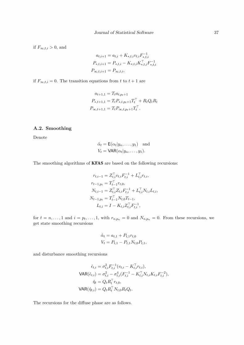
Journal of Statistical Software 37
if F∞,t,i > 0, and
at,i+1 = at,i +K∗,t,ivt,iF−1∗,t,i
P∗,t,i+1 = P∗,t,i −K∗,t,iK>∗,t,iF−1∗,t,i
P∞,t,i+1 = P∞,t,i,
if F∞,t,i = 0. The transition equations from t to t+ 1 are
at+1,1 = Ttat,pt+1
P∗,t+1,1 = TtP∗,t,pt+1T>t +RtQtRt
P∞,t+1,1 = TtP∞,t,pt+1T>t .
A.2. Smoothing
Denoteαt = E(αt|yn, . . . , y1) andVt = VAR(αt|yn, . . . , y1).
The smoothing algorithms of KFAS are based on the following recursions:
rt,i−1 = Z>t,ivt,iF−1t,i + L>t,irt,i,
rt−1,pt = T>t−1rt,0,
Nt,i−1 = Z>t,iZt,iF−1t,i + L>t,iNt,iLt,i,
Nt−1,pt = T>t−1Nt,0Tt−1,
Lt,i = I −Kt,iZ>t,iF
−1t,i ,
for t = n, . . . , 1 and i = pt, . . . , 1, with rn,pn = 0 and Nn,pn = 0. From these recursions, weget state smoothing recursions
αt = at,1 + Pt,1rt,0
Vt = Pt,1 − Pt,1Nt,0Pt,1,
and disturbance smoothing recursions
εt,i = σ2t,iF
−1t,i (vt,i −K>t,irt,i),
VAR(εt,i) = σ2t,i − σ4
t,i(F−1t,i −K
>t,iNt,iKt,iF
−2t,i ),
ηt = QtR>t rt,0,
VAR(ηt,i) = QtR>t Nt,0RtQt.
The recursions for the diffuse phase are as follows.
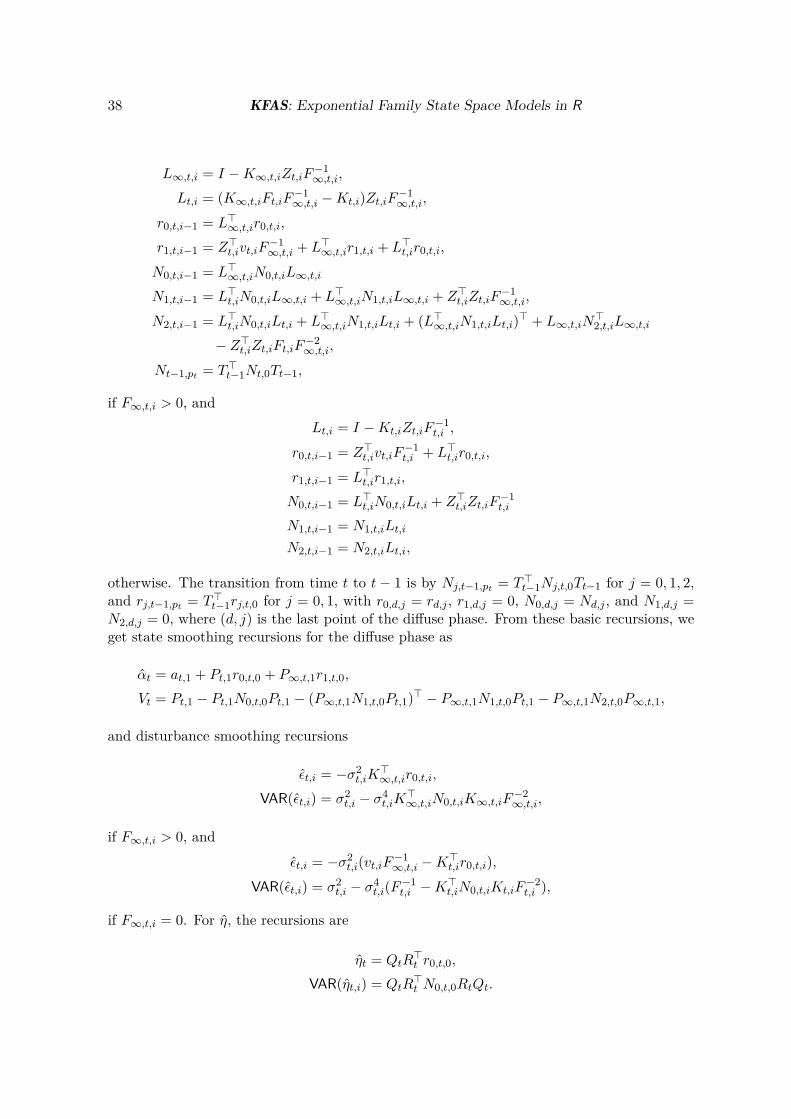
38 KFAS: Exponential Family State Space Models in R
L∞,t,i = I −K∞,t,iZt,iF−1∞,t,i,
Lt,i = (K∞,t,iFt,iF−1∞,t,i −Kt,i)Zt,iF−1
∞,t,i,
r0,t,i−1 = L>∞,t,ir0,t,i,
r1,t,i−1 = Z>t,ivt,iF−1∞,t,i + L>∞,t,ir1,t,i + L>t,ir0,t,i,
N0,t,i−1 = L>∞,t,iN0,t,iL∞,t,i
N1,t,i−1 = L>t,iN0,t,iL∞,t,i + L>∞,t,iN1,t,iL∞,t,i + Z>t,iZt,iF−1∞,t,i,
N2,t,i−1 = L>t,iN0,t,iLt,i + L>∞,t,iN1,t,iLt,i + (L>∞,t,iN1,t,iLt,i)> + L∞,t,iN>2,t,iL∞,t,i
− Z>t,iZt,iFt,iF−2∞,t,i,
Nt−1,pt = T>t−1Nt,0Tt−1,
if F∞,t,i > 0, andLt,i = I −Kt,iZt,iF
−1t,i ,
r0,t,i−1 = Z>t,ivt,iF−1t,i + L>t,ir0,t,i,
r1,t,i−1 = L>t,ir1,t,i,
N0,t,i−1 = L>t,iN0,t,iLt,i + Z>t,iZt,iF−1t,i
N1,t,i−1 = N1,t,iLt,i
N2,t,i−1 = N2,t,iLt,i,
otherwise. The transition from time t to t− 1 is by Nj,t−1,pt = T>t−1Nj,t,0Tt−1 for j = 0, 1, 2,and rj,t−1,pt = T>t−1rj,t,0 for j = 0, 1, with r0,d,j = rd,j , r1,d,j = 0, N0,d,j = Nd,j , and N1,d,j =N2,d,j = 0, where (d, j) is the last point of the diffuse phase. From these basic recursions, weget state smoothing recursions for the diffuse phase as
αt = at,1 + Pt,1r0,t,0 + P∞,t,1r1,t,0,
Vt = Pt,1 − Pt,1N0,t,0Pt,1 − (P∞,t,1N1,t,0Pt,1)> − P∞,t,1N1,t,0Pt,1 − P∞,t,1N2,t,0P∞,t,1,
and disturbance smoothing recursions
εt,i = −σ2t,iK
>∞,t,ir0,t,i,
VAR(εt,i) = σ2t,i − σ4
t,iK>∞,t,iN0,t,iK∞,t,iF
−2∞,t,i,
if F∞,t,i > 0, and
εt,i = −σ2t,i(vt,iF−1
∞,t,i −K>t,ir0,t,i),
VAR(εt,i) = σ2t,i − σ4
t,i(F−1t,i −K
>t,iN0,t,iKt,iF
−2t,i ),
if F∞,t,i = 0. For η, the recursions are
ηt = QtR>t r0,t,0,
VAR(ηt,i) = QtR>t N0,t,0RtQt.

Journal of Statistical Software 39
Affiliation:Jouni HelskeUniversity of JyväskyläDepartment of Mathematics and Statistics40014 Jyväskylä, FinlandE-mail: [email protected]
Journal of Statistical Software http://www.jstatsoft.org/published by the Foundation for Open Access Statistics http://www.foastat.org/
June 2017, Volume 78, Issue 10 Submitted: 2015-05-06doi:10.18637/jss.v078.i10 Accepted: 2016-06-15