Keyword Search Advertising and Limited Budgetsbear.warrington.ufl.edu/wshin/Woochoel_Shin/main...
33
Keyword Search Advertising and Limited Budgets Woochoel Shin University of Florida Woochoel Shin is an Assistant Professor of Marketing at Warrington College of Business Admin- istration, University of Florida, Gainesville, FL 32611; email: wshin@ufl.edu. The paper is partially based on the author’s doctoral dissertation at Duke University. The author thanks the Senior Ed- itor, the Associate Editor, two anonymous reviewers, Liang Guo, Maarten Janssen, Deb Mitra, Jiwoong Shin, Steve Shugan, Richard Staelin, Ruqu Wang, Ken Wilbur, Jinhong Xie, Huseyin Yildirim, and Kaifu Zhang for their helpful comments. The author is especially grateful to Wilfred Amaldoss and Preyas Desai, for their support and valuable discussion on the initial idea as well as earlier versions of the paper.
Transcript of Keyword Search Advertising and Limited Budgetsbear.warrington.ufl.edu/wshin/Woochoel_Shin/main...

Keyword Search Advertising and Limited Budgets
Woochoel ShinUniversity of Florida
Woochoel Shin is an Assistant Professor of Marketing at Warrington College of Business Admin-
istration, University of Florida, Gainesville, FL 32611; email: [email protected]. The paper is partially
based on the author’s doctoral dissertation at Duke University. The author thanks the Senior Ed-
itor, the Associate Editor, two anonymous reviewers, Liang Guo, Maarten Janssen, Deb Mitra,
Jiwoong Shin, Steve Shugan, Richard Staelin, Ruqu Wang, Ken Wilbur, Jinhong Xie, Huseyin
Yildirim, and Kaifu Zhang for their helpful comments. The author is especially grateful to Wilfred
Amaldoss and Preyas Desai, for their support and valuable discussion on the initial idea as well as
earlier versions of the paper.

Keyword Search Advertising and Limited Budgets
Abstract
In keyword search advertising, many advertisers operate on a limited budget. Yet how limited
budgets affect keyword search advertising has not been extensively studied. This paper offers an
analysis of the generalized second-price auction with budget constraints. We find that the budget
constraint may induce advertisers to raise their bids to the highest possible amount for two different
motivations: to accelerate the elimination of the budget-constrained competitor as well as to reduce
their own advertising cost. Thus, in contrast to the current literature, our analysis shows that both
budget-constrained and unconstrained advertisers could bid more than their own valuation. We
further extend the model to consider dynamic bidding and budget-setting decisions.
Keywords: Keyword Search Advertising, Budget Constraint, Generalized Second-Price Auction,
Online Advertising, Competitive Bidding Strategy, Analytical Model.

1
1 Introduction
Keyword search advertising has become a major form of online advertising with an annual
revenue of 18.4 billion dollars in the US (IAB 2013). In keyword search advertising, a
search query (or keyword) triggers a number of text-based advertisements, which are listed
according to the outcome of the generalized second-price auction. Given its growing prac-
tical importance, this new form of online advertising has drawn the attention of academic
researchers (Edelman et al. 2007, Varian 2007, Katona and Sarvary 2009). So far the lit-
erature has examined the mechanism of the generalized second-price auction, but without
considering the budget constraint of advertisers. However, in reality, advertisers do not have
unlimited resources allocated to search advertising. Recognizing this constraint, search en-
gines also explicitly ask advertisers to specify their daily spending limit. Therefore, it is
crucial to understand how budget constraints affect keyword search advertising. This paper
seeks to address this issue by examining the generalized second-price auction with budget
constraints.
In the absence of budget constraints, the extant models of the generalized second-price
auction suggest that advertisers will be listed in the order of valuations and that they will
likely bid as much as the marginal profit they could earn from the slot they take in equilibrium
(Varian 2007).1 In reality, however, a lower-valuation advertiser might be listed higher
than a higher-valuation advertiser (Jerath et al. 2011). Moreover, advertisers could turn
aggressive and bid beyond their marginal profit, even close to the higher-ranked competitor’s
bid (Ganchev et al. 2007). These aberrations motivate us to closely examine the impact of a
budget constraint on the bidding incentive of advertisers. Specifically, we seek answers to the
following questions: how does a budget constraint alter the bidding strategy of advertisers?
More importantly, what is the process by which a budget constraint affects the bidding
behavior? As a consequence of such a change, how will the equilibrium profits and the
equilibrium listing order be influenced? Also, how does the resulting equilibrium bid compare
with the per-click valuation?
1The generalized second-price auction has been proved to have multiple equilibria. Bidding as much asan advertiser’s own marginal profit is equivalent to bidding at the lower bound of these solutions, which wasshown to be consistent with the advertisers’ best locally envy-free equilibrium (Edelman et al. 2007) andwas also suggested as a reasonable bidding strategy following a compelling argument (Varian 2007).

2
To investigate these issues, we develop a model of the generalized second-price auction in
the context of keyword search advertising. In this model, advertisers compete for a slot in a
one-shot bidding game in order to generate clicks to their web site. They play a bidding game
with pre-specified budget constraints. We then extend the model to consider a two-period
bidding game and the budget-setting stage prior to the bidding game.
Our analysis first shows that in the presence of a budget constraint, advertisers are not
always listed in the order of valuations. We find that a budget-constrained advertiser may
concede a slot to a lower-valuation advertiser if its own budget is small. This is because with
a limited budget, the advertisement will be listed for a limited period of time and generate
a limited number of clicks, which makes the advertiser an inferior competitor.
Given the listing order, we also find that the presence of a budget-constrained advertiser
may motivate all lower-ranked advertisers to shift their bids to the highest possible amount
that they can bid in equilibrium. Given that in the generalized second-price auction, an
advertiser’s bid determines the cost of its higher-ranked competitor, this highest bid is set
such that it decreases their respective higher-ranked competitor’s profits to the level of the
profits the competitor would earn by moving down to the next slot. This implies that due
to the budget constraint of one advertiser, multiple advertisers listed below can experience
a profit squeeze, earning zero marginal profit in their current slot.
We identify two different mechanisms that drive the above result. First, advertisers
increase their bids to raise the cost of the higher-ranked competitor, but they do so only
when the competitor is budget-constrained. To see this, note that in the absence of a budget
constraint, increasing the bid and thus the cost of the competitor has no bearing on the
advertiser’s own profits. However, if a higher-ranked advertiser is budget-constrained, raising
the cost of this competitor can accelerate the depletion of its budget. After the competitor
exhausts its budget and thus drops out of the auction, all advertisers listed below can move
up by a slot, collect more clicks at the same per-click price, and earn additional profits. Given
this, the advertiser listed immediately below a budget-constrained advertiser is motivated
to increase its own bid, since its bid directly affects the cost of the budget-constrained
competitor. Interestingly, the budget constraint can also motivate distant advertisers in
even lower slots to bid more. This is because an equilibrium bid in the generalized second-
price auction is affected by the lower-ranked advertiser’s bid, and any bid increase of distant

3
advertisers can ripple through the list of higher-ranked advertisers. This way, even distant
advertisers can contribute to the earlier elimination of the budget-constrained competitor,
which in turn helps them to improve their own profits. Thus, they will raise their bids as
high as possible in equilibrium.
Second, when the competitor is budget-constrained, an advertiser may reduce its own
cost by bidding more. This will be the case when an advertiser, say Advertiser i, takes the
slot right next to a budget-constrained competitor. As shown above, due to this higher-
ranked competitor’s budget constraint, another competitor below Advertiser i will raise its
bid until Advertiser i’s profits decrease to the level of profits it would earn at the next slot.
Advertiser i, by increasing its own bid, can improve this hypothetical next-slot profit, because
its bid prompts the higher-ranked competitor’s elimination from the auction. Therefore,
when Advertiser i increases its own bid and thus its own hypothetical next-slot profit, the
competitor below Advertiser i is left with less room to squeeze Advertiser i’s profits. This
results in a lower bid of the next-ranked competitor, leading to a smaller cost for Advertiser
i. Thus, Advertiser i can increase its bid with the purpose of reducing its own cost.
To assess the equilibrium implications of a budget constraint, we examine the equilibrium
bids of the budget-constrained advertiser as well as those of others. We find that advertisers
listed below a budget-constrained advertiser may set their bids higher than the valuation
when the slots are sufficiently heterogeneous in terms of click-through rates. To see this,
first note that these advertisers can increase their bids until their respective higher-ranked
competitor earns no more profits at the current slot than the next slot. Since greater hetero-
geneity among slots implies greater difference in profits across slots, advertisers have more
room to increase their bids, even beyond their valuation. Interestingly, even the budget-
constrained advertiser can bid at least as high as its own valuation if it takes the last slot.
Denote such an advertiser by Advertiser N . Due to Advertiser N ’s budget constraint, the
next-ranked advertiser in equilibrium sets its bid such that Advertiser N does not earn any
more profits than those of losing the last slot, in which case it obtains zero profits. This
implies that the next-ranked competitor bids exactly the valuation of Advertiser N . In order
to win over this competitor, Advertiser N bids at least as high as the competitor’s bid, which
is its own valuation.
We also extend the model to examine two additional issues. First, our analysis of the
4
dynamic bidding decisions shows that the high-valuation advertiser may give up taking the
top slot in one period, not only when the budget is sufficiently small but also when it is
sufficiently large. We also examine the endogenous budget-setting decisions and find that
the low-valuation advertiser may voluntarily choose to be budget-constrained whereas the
high-valuation advertiser always chooses a budget large enough to cover the entire period.
Related Literature This paper studies the role of the budget constraint in keyword
search advertising and thus builds on the literature on keyword search advertising. Edelman
et al. (2007) and Varian (2007) pioneered theoretical research on search advertising by
developing an equilibrium concept specific to this context. Since then, both theoretical
and empirical researches have investigated issues on auction mechanisms (Balachander et
al. 2009, Zhu and Wilbur 2011, Jerath and Sayedi 2011, Amaldoss, Desai, and Shin 2014,
Amaldoss, Jerath, and Sayedi 2014), consumer search (Athey and Ellison 2011, Chen and
He 2011), listing order (Katona and Sarvary 2010, Jerath et al. 2011, Xu et al. 2011),
keyword choice (Desai et al. 2014, Rutz and Bucklin 2011, Rutz et al. 2011), measurement
and evaluation (Rutz et al. 2012), position effects (Agarwal et al. 2011), interaction with
organic results (Yang and Ghose 2010), interaction with other media (Joo et al. 2012),
advertising design (Rutz and Trusov 2011), dynamic bidding patterns (Zhang and Feng
2011), and click fraud (Wilbur and Zhu 2009). Surprisingly, most of these studies have
abstracted away from the issue of the budget constraint, with only a few exceptions (e.g.,
Amaldoss et al. 2014, Sayedi et al. 2014, Shin 2010, Wilbur and Zhu 2009). However, in
reality, most advertisers are subject to the budget constraint and may alter their strategies
due to their limited budgets. Thus, this work focuses on the role that the budget constraint
plays in keyword search advertising. In particular, we show that advertisers may shift their
bids from the lowest to the highest possible amount when faced with a budget-constrained
competitor. This helps us understand the aggressive bidding behavior that is often observed
in practice.
At the heart of such aggressive bidding strategies is the incentive to eliminate the com-
petitor from the auction in order to achieve long-term gains. The Raising Rivals’ Costs
(RRC) literature shares a similar idea (Shin 2009). The idea behind the RRC strategy is to
put competitors at a disadvantage by raising their costs and to obtain competitive advantage
in the market (Salop and Scheffman 1983). We have seen many applications of the RRC

5
strategy in the industrial organization theory, including exclusive dealing (Salop and Scheff-
man 1983, Krattenmaker and Salop 1986), vertical integration (Krattenmaker and Salop
1986, Ordover et al. 1990) and overbuying supply materials (Salop and Scheffman 1987), all
as an option of the stronger firm. In contrast, the current paper illustrates that in the con-
text of keyword search advertising, the cost-raising strategy is relevant not only for stronger
firms but also for weaker firms.
Based on a similar idea, Pitchik and Schotter (1988) and Benoit and Krishna (2001) have
investigated the aggressive bidding behavior in two sequential second-price auctions. They
show that the equilibrium bid of the first auction can be high due to their incentive to win
the second auction at a lower price. However, in the context of the single-unit second-price
auction, this discussion cannot go further than the immediate losing bidder. In contrast, in
our setting, the benefit of driving out a certain winner can be shared by multiple lower-ranked
bidders. Thus, our research provides a more nuanced discussion on the condition for this
aggressive bidding incentive to prevail. We also add some new findings that can be shown
only in the context of multi-item auctions. For example, in the generalized second-price
auction, the profits of multiple bidders can be negatively affected by the budget constraint
of one bidder, and even the budget-constrained bidder can bid beyond its own valuation.
More importantly, we identify another incentive for an aggressive bid even without any
intention to hurt the competitor, which is to reduce the bidder’s own cost. Such an incentive
has not been discussed in any literature and is specific to the generalized second-price auction
setting.
In the auction literature, there have been observations of overbidding behavior in various
contexts (for example, Coppinger et al. (1980) in the first-price auction; Kagel et al. (1987)
in the second-price auction; Che et al. (2011) in the generalized second-price auction).
Several explanations have been given for the phenomenon. Chen and Plott (1998) showed
that risk-averse bidders may overbid in the first-price auction. Cox et al. (1992) found
that the utility of winning can help better explain the overbidding data. In the second-
price auction, Kagel et al. (1987) ascribed overbidding to the illusion that overbidding may
increase the chance to win. Finally, Morgan et al. (2003) showed that spiteful bidding can
rationalize the overbidding in the second-price auction. The bidding pattern that we consider
in the current paper also involves aggressive bidding behavior, but it does not constitute a

6
behavioral aberration. On the contrary, aggressively bidding under a competitor’s budget
constraint is a profit-maximizing strategy. In addition, although such a strategy might
appear to involve spiteful motivation, we show that it can be rationalized as an act driven
by pure self-interest.
The rest of the paper is organized as follows. In the next section, we introduce our model.
We then provide a theoretical analysis of the model in Section 3. In section 4, we extend the
model in two ways and provide the analysis for each of these extensions. In the last section,
we conclude with a summary and directions for future research.
2 Model
In this section, we present a model of the generalized second-price auction in the context of
keyword search advertising. We first describe the participants and then present the rules of
the auction. Later we explain the equilibrium concept used in our model.
2.1 Participants
We consider a search engine who auctions off two advertising slots. As in reality, these slots
are sequentially listed and thus the first slot generates more clicks than the second slot for
the same advertiser. To capture this difference, we assume that the click-through rate of
an advertisement in the second slot is discounted by δ from that in the first slot. Thus,
without loss of generality, we represent the slot-specific click-through rates of the two slots
respectively by 1 (for the first slot) and 1− δ (for the second slot), where 0 < δ < 1.
In addition to the search engine, there are three advertisers in this market, denoted by
Firm H, Firm M and Firm L, who advertise on the search engine results page and thus
participate in this position auction.2 Through advertising, they aim to generate traffic to
their web site and thus strive to collect more clicks with the same advertising budget.
The three advertisers in our model are heterogeneous in their valuation for a click, which
we denote by vi, where i ∈ {H,M,L}. While this reflects the fact that some advertisers are
better than others at converting clicks into sales, we do not explicitly model this conver-
sion process but treat vi as an exogenous parameter, following the tradition of the search
2In this paper, advertisers are interchangeably referred to as firms or bidders.
7
advertising literature (See Varian 2007 and Edelman et al. 2007). Advertisers also vary in
their ability to generate clicks. Since some advertisers are more attractive or relevant to
consumers, they generate more clicks than others at the same slot. To represent this differ-
ence, we denote the advertiser-specific click-through rate (CTR) by ri, where i ∈ {H,M,L}.
Then Advertiser i’s click-through rate at the first slot is given by ri while that at the second
slot is (1 − δ)ri. By normalizing the number of impressions to one, we obtain the number
of clicks that Advertiser i generates as ri at the first slot and (1 − δ)ri at the second slot.
Given the heterogeneity among advertisers described thus far, we define the CTR-weighted
valuation as the product of the click-through rate and the valuation: rivi, where i ∈ {H,M,L}
and assume that the three advertisers are ordered by rHvH > rMvM > rLvL.
2.2 Generalized Second-Price Auction
In the generalized second-price auction for advertising slots, each advertiser submits its bid
for a click bi based on the valuation for a click vi (i = H,M,L). The search engine then
ranks the advertisers by their potential profitability, which is given by the product of their
click-through rate and the bid: {ribi}. We also call this a CTR-weighted bid. The generalized
second-price auction rule suggests that each advertiser is charged per click by the minimum
amount that allows them to take the current slot. In particular, if Advertiser i takes Slot j,
this advertiser has to pay per click, pij ≡r[j+1]b[j+1]
ri, where [j + 1] denotes the (j + 1)th-ranked
advertiser in terms of the CTR-weighted bid. Then the profit of Advertiser i when ranked
at jth position is given by:
Πij =
ri(vi − pi1) = rivi − r[2]b[2] when j = 1
(1− δ)ri(vi − pi2) = (1− δ)(rivi − r[3]b[3]) when j = 2
0 when j = 3
. (1)
Note that in this auction, there exists a minimum bid C0 in units of the CTR-weighted bid.
If an advertiser drops out of the auction for any reason, there might be no advertiser below
Advertiser i, in which case, the payment of Advertiser i is determined by this minimum bid,
that is, ripij = C0. We assume C0 < rLvL.
Each advertiser may be financially constrained. For this possibility, let Ki (i = H,M,L)
denote Advertiser i’s budget for the auction. We assume that the budgets are specified by
factors exogenous to the model. Later in a model extension, we also consider the endogenous

8
choice of the budget by each advertiser (See Section 4.2). Given Ki, Firm i’s budget constraint
is defined to be binding when Ki is less than the total cost that Firm i would incur if it stayed
in the auction for the entire period.3 Thus, when Firm i’s budget constraint is binding, the
advertisement of Firm i is shown at Slot j only for a fraction of the period ( Kiripij
at the first
slot and Ki(1−δ)ripij at the second slot), after which the lower-ranked advertisers’ advertisements
move up by one slot.4 When the budget constraint is not binding, since the budget is greater
than the potential payment, the advertisement will be shown for the entire period. Finally,
when both Firm i and Firm i′ have binding budget constraints, Firm i is said to be more
budget-constrained if Firm i’s advertisement would be shown for a shorter period than that
of Firm i′ in their respective slots.
2.3 Equilibrium Concept
We model the bidding game among advertisers as a one-shot, complete information game.
This game structure reflects the long-term stabilized state of the bidding game and thus
captures the essence of the competition for the slots while abstracting away from the dynamic
aspect that is less essential to the decision problem (See Katona and Sarvary 2007, and Jerath
et al. 2011 for similar assumptions; and also Varian 2007 and Edelman and Schwarz 2010
for similar arguments regarding this assumption). However, to examine the impact of the
dynamic decisions on the bidding equilibrium, in Section 4.1, we offer a model extension
where we allow for changes in bids across the two periods. In these games, we derive a
Symmetric Nash Equilibrium, where no firm has an incentive to switch its slot with any
other firm (Varian 2007). Since this equilibrium concept results in multiple equilibria, we
further refine it by focusing on the Pareto-dominant equilibrium, which is derived as the
lower bound of the equilibrium bid for every firm. The lower bound solution is viewed as
the compelling equilibrium in the literature (Varian 2007).
3Since the cost varies with the slot a firm takes, the binding budget constraint is defined for a pair ofa firm and a slot. However, whenever the slot can be explicitly or implicitly fixed, we define the budgetconstraint of a firm without specifying a slot.
4In reality, search engines provide an option to spread the display of the advertisement throughout theentire period. Thus, at any point in the period, the advertisement is shown with a probability Ki
ripij(at the
first slot) or Ki
(1−δ)ripij (at the second slot). In either case, by observing the frequency of the display of the
competitor’s advertisement, each advertiser can correctly infer the advertising budget of the competitor.
9
3 Analysis
In this section, we provide an analysis of our model with a focus on the impact of the budget
constraint in keyword search advertising. For this purpose, we first establish the benchmark
by examining a case in which no advertiser has a limited budget. Then we investigate the
impact of limited budgets by considering the budget constraint of Firm H, Firm M, and both
in order.
3.1 No Budget Constraint
Suppose no firm has a binding budget constraint and the equilibrium listing order is given
as H-M-L. Then the Symmetric Nash Equilibrium implies that Firm H cannot earn more
profits by moving down to the second slot. Using the profits given in (1), we have
ΠH1 = rHvH − rM bM ≥ ΠH2 = (1− δ)(rHvH − rLbL). (2)
At the same time, Firm M should not earn more profits by switching its slot with Firm H
or Firm L. This leads to the following conditions:
ΠM2 = (1− δ)(rMvM − rLbL) ≥ ΠM1 = rMvM − rM bM (3)
ΠM2 = (1− δ)(rMvM − rLbL) ≥ ΠM3 = 0. (4)
Note that when Firm M deviates to the first slot, its payment is given by rM bM , and not by
rHbH . This is because the deviation from the Symmetric Nash Equilibrium involves switching
positions while keeping the payment the same on each position (See Varian 2007 for more
clarification). Finally, in equilibrium, Firm L cannot earn more profits by moving up to the
second slot:
ΠL3 = 0 ≥ ΠL2 = (1− δ)(rLvL − rLbL). (5)
These inequalities imply that Firm M and Firm L’s equilibrium bids are bounded as follows:
δrMvM + (1− δ)rLbL ≤ rM bM ≤ δrHvH + (1− δ)rLbL (6)
rLvL ≤ rLbL ≤ rMvM . (7)
In addition, the ranking determination rule of the auction implies
rHbH ≥ rM bM . (8)
10
While any combination of bids satisfying (6)-(8) makes every firm stay at the current slot and
thus constitutes a Symmetric Nash Equilibrium, we focus on the following Pareto-dominant
equilibrium (i.e., the lower-bound solution):
b∗L = vL (9)
b∗M = δvM + (1− δ) rLvLrM(10)
b∗H = δ rMvMrH+ (1− δ) rLvLrH
. (11)
It is worthwhile to note that the equilibrium bids of Firm M and Firm L given in (9) and (10)
are obtained by equating their own profits in the current slot to the deviation profits in the
upper slot; that is, equating the two sides of inequalities given in (3) and (5). This implies
that both firms choose to bid the marginal profit they would earn by moving up by one slot.
Since the bid is based on their willingness to pay for the higher slot, this is a reasonable
bidding strategy for advertisers to follow (See Jerath et al. 2011 for similar interpretation).
Finally, note that the equilibrium listing order without any binding budget constraint
is always given as H-M-L.5 This is because a firm with higher CTR-weighted valuation can
generate greater additional profits from the additional clicks obtained from the higher slot
compared to the lower slot. Then, according to the aforementioned bidding strategy of the
Pareto-dominant equilibrium, the firm with higher CTR-weighted valuation will bid higher
and thus win the higher slot (See also Varian 2007). We next consider the cases with binding
budget constraints.
3.2 Firm H’s Budget Constraint
Suppose Firm H’s budget constraint is binding at the first slot while the other firms are not
budget-constrained (i.e., (1− δ)rLvL < KH < δrMvM + (1− δ)rLvL and Ki ≥ δrMvM + (1− δ)rLvL,
i = M,L). As shown in the previous section, the equilibrium listing order among advertisers
without binding budget constraints is determined by the order of CTR-weighted valuations.
Since Firm H’s budget constraint is binding only at the first slot, the listing orders other
than H-M-L or M-H-L cannot be observed in equilibrium. In fact, in contrast with the
5To see this, replace H, M, and L, respectively by [1], [2], and [3], in inequalities given in (2)-(5). Then,adding (2) and (3) side by side results in r[1]v[1] ≥ r[2]v[2] while adding (4) and (5) side by side leads tor[2]v[2] ≥ r[3]v[3]. Since rHvH > rMvM > rLvL, these suggest that in equilibrium, Firm H takes the first slot,Firm M takes the second slot, and Firm L does not take any slot.

11
previous case, both H-M-L and M-H-L can be observed in equilibrium. More specifically,
M-H-L becomes an equilibrium listing order if Firm H is heavily budget-constrained at the
first slot, i.e., if KH is small enough (See Claim A1 in the online Appendix for proof). This is
because Firm H’s budget constraint shortens the period that Firm H stays in the auction at
the first slot and thus decreases the actual number of clicks that Firm H could obtain. This
in turn decreases the effective CTR-weighted valuation for Firm H at the first slot, causing
Firm H to lose the first slot to Firm M. Thus, the equilibrium listing order in this case is not
always consistent with the order of CTR-weighted valuations. However, moving forward, we
focus on the order of H-M-L for the purpose of the illustration, relegating the analysis of the
other case to the online Appendix.
When Firm H takes the first slot, it participates in the auction while its budget lasts, but
drops out afterwards. Thus, for the KHrM bM
fraction of the period, Firm H takes the first slot
while Firm M gets the second. For the rest (i.e., 1− KHrM bM
of the period), only Firm M and
Firm L participate and take the first and the second positions respectively. When Firm L
takes the second slot, since there is no other advertiser below it, the payment is given by the
minimum bid C0. In this case, the incentive compatibility conditions are given as follows:
ΠH1 =(
KHrMbM
)rHvH−KH ≥ ΠH2 = (1− δ)(rHvH − rLbL) (12)
ΠM2 ={(
KHrMbM
)(1−δ)+
(1− KH
rMbM
)}(rMvM−rLbL) ≥ ΠM1 = rMvM − rM bM (13)
ΠM2 ={(
KHrMbM
)(1−δ)+
(1− KH
rMbM
)}(rMvM−rLbL) ≥ ΠM3 =
(1− KH
rMbM
)(1−δ)(rMvM−C0) (14)
ΠL3 =(
1− KHrMbM
)(1−δ)(rLvL−C0) ≥ ΠL2 =
{(KH
rMbM
)(1−δ)+
(1− KH
rMbM
)}(rLvL−rLbL)(15)
Note that when Firm M switches its position with Firm L in deviation, Firm L pays rM bM
and thus Firm H is still budget-constrained and drops out after a(
KHrM bM
)fraction of the
period (See the right-hand side of (14) and (15)). By simple inspection, it is easy to see
that (12) determines the upper bound while (13) gives the lower bound of bM . In this
case, however, every bid between these two bounds cannot be an equilibrium bid for Firm
M. This is because Firm M’s profit at the second slot increases with its own bid: ∂ΠM2∂bM
=
( KHrM b
2M
)δ(rMvM − rLbL) > 0.6 Thus in equilibrium, Firm M makes its bid uniquely at the upper
6More precisely, we need to check the total derivative dΠM2
dbM, given that in equilibrium, bM can also affect
ΠM2 through bL. We show later that dΠM2
dbM= ∂ΠM2
∂bL
∂bL(bM )∂bM
+ ∂ΠM2
∂bM> 0 indeed holds.

12
bound solution:
bM (bL) = rHvHKHrM{KH+(1−δ)(rHvH−rLbL)} (16)
We also note here that this solution is obtained by equating Firm H’s profit in the first slot
to that in the second slot, i.e., the two sides of (12). This implies that Firm M chooses to
bid such that at the first slot, Firm H cannot earn any more profits than what it would earn
in the second slot.
Similarly, focusing on Firm L’s bid, observe that, given ΠL3 in (15) and bM (bL) in (16),
dΠL3dbL
= ∂ΠL3∂bL
+ ∂ΠL3∂bM
∂bM (bL)∂bL
= 0 + (1− δ)(rLvL − C0)(
KHrM b
2M
)((1−δ)rHvHrLKH
rM{KH+(1−δ)(rHvH−rLbL)}2)> 0, (17)
which implies that Firm L’s profit (i.e., ΠL3) increases with its own bid. Thus, although (14)
and (15) respectively define the upper bound and the lower bound of bL, the equilibrium bid
is uniquely determined at the upper bound, as the following:
bL(bM ) ={(1−δ)C0+δrMvM}(rM bM−KH)+(1−δ)rMvMKH
rL(rM bM−δKH)(18)
Again, this solution, since it equates the two sides of (15), suggests that Firm M makes no
additional profits at the second rank compared to the third. Finally, given ΠM2 in (13) and
bL(bM ) in (18), we confirm that
dΠM2dbM
= ∂ΠM2∂bL
∂bL(bM )∂bM
+ ∂ΠM2∂bM
(19)
= rL
{(KH
rMbM
)(1−δ)+
(1− KH
rMbM
)}{(1−δ)2rM (rMvM−C0)KH
rL(rMbM−δKH )2
}+
(δKHrMb2
M
)(rMvM−rLbL)>0
holds.7
This analysis, together with the one in the previous section, leads to the following propo-
sition. All proofs can be found in the Appendix.
Proposition 1. An advertiser’s budget constraint motivates lower-ranked advertisers to shift
their bids from the lowest to the highest possible amount.
7More formally, suppose dΠM2
dbM≤ 0. Then Firm M’s optimal bid is determined either at the lower bound
by (13) or at any constant between the two bounds, but at these solutions, it is easy to see that ∂bM (bL)∂bL
≥ 0
holds and thus, we have dΠL3
dbL= ∂ΠL3
∂bL+ ∂ΠL3
∂bM
∂bM (bL)∂bL
≥ 0. This implies that Firm L’s optimal bid is givenas in (18), i.e., the upper bound, or as any constant between the two bounds. In either case, (19) holdstrue, but this is a contradiction. Therefore in equilibrium, we always have dΠM2
dbM> 0. In addition, by (17),
dΠL3
dbL> 0 also holds. Lastly, the equilibrium bids are derived by simultaneously solving (16) and (18). This
derivation as well as the equilibrium condition is reported in the Appendix (see the proof of Proposition 2).

13
The proposition shows how a budget constraint may alter the equilibrium bidding strategy
of advertisers. In the absence of the budget constraint, advertisers bid the lower bound of all
bids satisfying the incentive compatibility conditions, in the Pareto-dominant equilibrium.
In the presence of the budget constraint, however, the advertisers listed below the budget-
constrained advertiser raise their bids to the upper bound.
To see the intuition for this result, note that when the budget-constrained advertiser
exhausts its budget, it drops out of the auction. Whenever this happens, all the lower-
ranked advertisers move up by one slot, collect more clicks at the same per-click price, and
thus earn additional profits. These additional profits will be further increased if the budget-
constrained advertiser can be removed earlier from the auction. Recall that in the generalized
second-price auction, the per-click price is determined by the next-highest bid. Hence the
time for which a budget-constrained advertiser lasts in the auction can be affected by the
bid of the adjoining lower-ranked advertiser. This creates an incentive for the immediately
lower-ranked advertiser to increase its own bid, with the purpose of increasing the cost of
the budget-constrained competitor and thus accelerating the removal of this competitor.
For the very same reason, the distant lower-ranked advertisers also have an incentive to
increase theirs bids. To see this, note that in the generalized second-price auction, an equi-
librium bid is affected by the lower-ranked advertiser’s bid. Thus, the increase in any lower-
ranked advertiser’s bid ripples through a series of higher-ranked advertisers and eventually
raises the cost of the budget-constrained advertiser. Even though the adjoining lower-ranked
advertiser may increase its own bid up to its maximum, the bid of any distant lower-ranked
advertiser could further lift it up by raising that maximum. This implies that even distant
advertisers can contribute to the earlier elimination of the budget-constrained competitor,
which in turn helps them to improve their own profits. Therefore, all the lower-ranked ad-
vertisers, immediate or distant, are motivated to increase their bids as high as possible in
order to accelerate the elimination of a budget-constrained advertiser.8
Notice that the incentive compatibility conditions imply that the upper bound of each ad-
vertiser’s bid is determined such that the adjoining higher-ranked advertiser has no incentive
8To be more precise, this holds for all lower-ranked advertisers that are not budget-constrained. Thisresult is in contrast with the findings in the generalized second-price auctions, where a bidder’s budgetconstraint initiates the cost-raising incentive of the adjoining lower-ranked bidder only (See Pitchik andSchotter 1988 and Benoit and Krishna 2001).

14
to move down to the lower slot. In other words, the equilibrium bid makes the higher-ranked
competitor earn as much profit as that obtained at the adjacent lower slot. Since the cost-
raising incentive can be found in all advertisers below the budget-constrained advertiser,
this implies that not only the budget-constrained advertiser but also other advertisers listed
below will lose all the marginal profits at their current slot.
However, we cannot obtain such results in the absence of a budget-constrained advertiser.
This is because the bid of an advertiser no longer affects the duration of any other firm’s
advertisement. Thus, raising the cost of a competitor by bidding more has no bearing on
the advertiser’s own profits. This implies that the budget constraint is a necessary condition
for advertisers to bid at the upper bound of all available bids in equilibrium.
Now one may wonder whether the equilibrium bid can even be higher than the valuation.
Note that in the absence of the budget constraint, it has been shown that the equilibrium
bids are not always truthful in the generalized second-price auction (Edelman et al. 2007).
Especially, as illustrated in (10), in the Pareto-dominant equilibrium, advertisers typically
bid lower than their own valuation. In contrast to this common view, we have the following
result.
Proposition 2. Advertisers may bid more than their valuation when the click-through rates
of advertising slots are sufficiently different and a competing advertiser is budget-constrained.
To understand the proposition, consider an advertiser that is ranked lower than a budget-
constrained advertiser. As noted earlier, in equilibrium, this advertiser increases its own bid
and thus the cost of the higher-ranked competitor, until the competitor loses all the additional
benefits of taking the higher slot. As the advertising slots become more heterogeneous in
terms of the click-through rate, these additional benefits increase and thus the equilibrium bid
necessary to make the competitor break even at its current slot also increases. Therefore, if
the click-through rates are sufficiently different, the equilibrium bid will be so high that it can
be even greater than the valuation. This result suggests that although the generalized second-
price auction does not always induce truthful bidding, it could achieve a better outcome for
the search engine in the presence of a budget-constrained advertiser. In particular, the
search engine could improve its own profitability by properly designing the distribution of
the click-through rates across the advertising slots.

15
So far we have focused attention on the case where Firm H is budget-constrained. In the
next section, we examine the impact of the budget constraint of another advertiser, Firm M.
3.3 Firm M’s Budget Constraint
In this section, we consider the case where Firm M’s budget constraint is binding at the
second slot. Specifically, suppose (1 − δ)C0 < KM < (1 − δ)rLvL but Ki > δrMvM + (1 − δ)rLvL
(i = H,L). In this case, as we show in the online Appendix, the equilibrium listing order
is always H-M-L (See Claim A2). Given this order, due to its budget constraint, Firm M
stays in the second slot for the KM(1−δ)rLbL period, after which it drops out and Firm L replaces
Firm M in the second slot. Even when deviating to the first slot, Firm M is also budget-
constrained and thus participates in the auction only for the KMrM bM
of the period and then the
top slot is taken by Firm H. Based on this discussion, the incentive compatibility conditions
are given as follows:
ΠH1=rHvH−
(KM
(1−δ)rLbL
)rMbM−
(1− KM
(1−δ)rLbL
)rLbL ≥ ΠH2=
{(KMrMbM
)(1−δ)+
(1− KM
rMbM
)}(rHvH−rLbL)(20)
ΠM2 =(
KM(1−δ)rLbL
)(1−δ)rMvM−KM ≥ ΠM1 =
(KMrMbM
)rMvM−KM (21)
ΠM2 =(
KM(1−δ)rLbL
)(1−δ)rMvM−KM ≥ ΠM3 = 0 (22)
ΠL3 =(
1− KM(1−δ)rLbL
)(1−δ)(rLvL−C0) ≥ ΠL2 = (1− δ)(rLvL − rLbL) (23)
While (22) and (23) respectively determine the upper bound and the lower bound of bL, since
dΠL3dbL
= ∂ΠL3∂bL
+ ∂ΠL3∂bM
∂bM∂bL
=(KMrLb
2L
)(rLvL − C0) + 0 > 0, (24)
Firm L’s optimal bid amount is determined at the upper bound, defined by (22):
b∗L = rMvMrL
. (25)
As before, at this solution, Firm M earns no more profits in the second slot than when it
does not take any slot. In contrast, since dΠM2dbM
= ∂ΠM2∂bM
+ ∂ΠM2∂bL
∂bL∂bM
= 0, any bid satisfying
(20) and (21) can be an equilibrium bid for Firm M. Taking the lower bound solution as the
Pareto-dominant equilibrium bid, we have
b∗M =rLb∗L
rM= vM . (26)

16
Note that at this set of solutions, all the incentive compatibility conditions in (20)-(23)
always hold. Thus, H-M-L is always an equilibrium listing order.
This analysis confirms the generality of Proposition 1 by showing that even the budget
constraint of any mid-ranked advertiser may also induce other advertisers to push their bids
upwards. It also confirms that the budget constraint does not alter the bidding behavior
of any higher-ranked advertiser. However, as shown in (26), even without any budget-
constrained advertiser at a higher slot, an advertiser may still bid high in equilibrium. The
following proposition presents such a case.
Proposition 3. When a budget-constrained advertiser takes the last slot, its equilibrium bid
is at least as high as the valuation.
Recall from the previous section that the (Pareto-dominant) equilibrium bid is determined
at the lower bound of all bids satisfying the incentive compatibility condition, if no higher-
ranked advertiser is budget-constrained. The proposition shows that even this lower-bound
solution can be as high as the valuation. To see this, consider an advertiser occupying the
last slot, which is also budget-constrained (denote it by Advertiser N). This advertiser will
earn zero profit when it moves down by one rank since there is no slot below. At the same
time, since it is budget-constrained, according to Proposition 1, the lower-ranked competitor
will bid high enough so that Advertiser N earns zero profits (i.e., the profits that accrue at
the next rank). This means that the bid of the lower-ranked competitor will be set exactly
at the valuation of Advertiser N in equilibrium. Then Advertiser N , to win the last slot,
has to bid weakly higher than its own valuation. Therefore, an advertiser, even when it
does not have any incentive to raise its bid, may be induced to bid at least as high as the
valuation. This is because the lower-ranked competitor’s cost-raising incentive pushes the
focal advertiser’s bid upwards as well.
3.4 Multiple Firms’ Budget Constraints
So far we have considered cases where only one firm has a binding budget constraint. In this
section, to complete our analysis, we consider multiple firms’ budget constraints. Given that
this case includes various subcases, we do not derive the equilibrium for every possible case
but only present one example of such cases for the purpose of the illustration. In particular,

17
we consider the case where both Firm H and Firm M are budget-constrained in the first
and the second slot, respectively.9 In this case, as shown in the online Appendix, only the
following two listing orders can be observed in equilibrium: H-M-L and H-L-M (See Claim
A3). Consistent with our earlier findings, this shows that a budget-constrained advertiser
(Firm M) can be ranked lower than its lower-valuation but unconstrained competitor (Firm
L) in equilibrium. It also implies that an advertiser budget-constrained at both slots (Firm
M) can never win over the competitor budget-constrained only at one slot (Firm H).10
Among the two listing orders, in this section, we only focus on H-M-L, since we are primarily
interested in the case where multiple firms are budget-constrained in equilibrium.11
Now suppose the equilibrium listing order is H-M-L. Further suppose Firm H is more
budget-constrained than Firm M in that Firm H drops out earlier, and let l denote the
duration of the period that Firm M stays in the auction after Firm H drops out. Then Firm
M takes the second slot for KHrM bM
fraction of the period but moves up to the first slot for l
fraction. Since Firm M’s total advertising cost amounts to its budget, we have(KHrM bM
)(1− δ)rLbL + l · rLbL = KM , (27)
which is equivalent to
l = KMrLbL
− (1− δ) KHrM bM
. (28)
Then, Firm M’s equilibrium profit under the H-M-L order is
ΠM2 =(
KHrM bM
)(1− δ)rMvM + l · rMvM −KM =
(KMrLbL
)rMvM−KM . (29)
Moving attention to Firm L, we note that even Firm L can take the second slot (for l
fraction of the period) and the first slot (for 1 − l − KHrM bM
fraction) due to drop-outs of the
other firms. Thus, Firm L’s profit under the H-M-L order is
ΠL3 = l(1− δ)(rLvL − C0) +(
1− l − KHrM bM
)(rLvL − C0) =
{1−δ KM
rLbL−(1−δ+δ2)
KHrMbM
}(rLvL−C0). (30)
9This corresponds to (1− δ)rLvL < KH < δrMvM + (1− δ)rLvL and (1− δ)C0 < KM < (1− δ)rLvL.10This is because at any set of bids, Firm M weakly prefers to take the second slot to the first slot, given
that it will exhaust all of its budget at both slots but collect more clicks at the second slot since it pays alower per-click cost. In contrast, there exists a set of bids at which Firm H is willing to take the first slotwhile Firm M takes the second slot.
11The other equilibrium listing order, H-L-M, involves only one firm budget-constrained in equilibriumand thus the analysis of such a case is essentially identical to that in previous sections. Also note that allthe rest listing orders, M-H-L, M-L-H, L-H-M, and L-M-H, cannot be observed in equilibrium. We providethe details of this analysis in Claim A3 of the online Appendix.

18
Based on these profits, the incentive compatibility conditions are given as follows:12
ΠH1=
(KH
rMbM
)rHvH−KH ≥ ΠH2=
{(KMrMbM
)(1−δ)+
(1− KM
rMbM
)}(rHvH−rLbL) (31)
ΠM2=
(KMrLbL
)rMvM−KM ≥ ΠM1=
(KMrMbM
)rMvM−KM (32)
ΠM2=
(KMrLbL
)rMvM−KM ≥ ΠM3=
(1− KH
rMbM
)(1−δ)(rMvM−C0) (33)
ΠL3=
{1−δ KM
rLbL−(1−δ+δ2)
KHrMbM
}(rLvL−C0) ≥ ΠL2=
{(KH
rMbM
)(1−δ)+
(1− KH
rMbM
)}(rLvL−rLbL) (34)
Note that the upper bound and the lower bound of bM are respectively defined by (31) and
(32), while those of bL are determined by (33) and (34) respectively.
We now examine the bidding strategy of both firms. First, suppose dΠM2dbM
≤ 0. Then
Firm M’s optimal bid is determined either at the lower bound by (32): bM (bL) = bL or at
any constant between the two bounds, which leads to ∂bM (bL)∂bL
≥ 0. In this case, we have
dΠL3dbL
= ∂ΠL3∂bL
+ ∂ΠL3∂bM
∂bM (bL)∂bL
> 0, since (30) suggests both ∂ΠL3∂bM
> 0 and ∂ΠL3∂bL
> 0. Thus, Firm
L’s optimal bid is determined at the upper bound by equating the two sides of (33):
bL(bM ) = rMvMrM bMKMrL{rM bMKM+(1−δ)(rMvM−C0)(rM bM−KH)} , (35)
which implies ∂bL(bM )∂bM
=− (1−δ)rMvM (rMvM−C0)KMKH{rMbMKM+(1−δ)(rMvM−C0)(rMbM−KH )}2
<0. Since (29) suggests both ∂ΠM2∂bM
=
0 and ∂ΠM2∂bL
< 0, this leads to dΠM2dbM
= ∂ΠM2∂bM
+ ∂ΠM2∂bL
∂bL(bM )∂bM
> 0, which is a contradiction. There-
fore, we always have dΠM2dbM
> 0 in equilibrium.
Given dΠM2dbM
> 0, Firm M bids its upper bound solution given by (31):
bM (bL) =rHvHKH+δKM (rHvH−rLbL)
rM (rHvH−rLbL+KH), (36)
Then it is easy to see that ∂bM (bL)∂bL
=KHrL(rHvH−δKM )
rM (rHvH−rLbL+KH)2 > 0, and this, together with ∂ΠL3∂bM
> 0
and ∂ΠL3∂bL
> 0, implies that dΠL3dbL
= ∂ΠL3∂bL
+ ∂ΠL3∂bM
∂bM (bL)∂bL
> 0.
This analysis shows that Firm L has an incentive to increase its bid, which is motivated by
both Firm H and Firm M’s budget constraints (i.e., ∂ΠL3∂bM
∂bM (bL)∂bL
> 0 for the former; ∂ΠL3∂bL
> 0
for the latter). This suggests that, as noted earlier, a lower-ranked advertiser, either adjoin-
ing or distant, may increase its bid to accelerate the elimination of the budget-constrained
advertiser. However, the partial derivative of Firm M’s profits (∂ΠM2∂bM
= 0) suggests that such
an incentive does not apply to Firm M’s case. In particular, although Firm M’s higher bid
12In our derivation of ΠM3, we assume KH
rMbM+ KM
(1−δ)rLbL ≥ 1, but this can be satisfied in equilibrium.
19
may accelerate the elimination of Firm H, Firm H’s earlier drop-out does not help increase
Firm M’s own profit. Still, Firm M bids the highest amount bounded by the incentive com-
patibility conditions, as suggested by the total derivative: dΠM2dbM
> 0. On investigating Firm
M’s motivation in this case, we obtain the following result.
Proposition 4. Bidding more may reduce an advertiser’s own cost.
The above analysis shows that Firm M has no incentive to raise the cost of Firm H and
yet increases its bid. The proposition suggests that we observe this because bidding more
could help Firm M to reduce its own advertising cost. To see how this might be the case,
consider an advertiser that is listed immediately below a budget-constrained advertiser.
For convenience, denote such an advertiser by Advertiser B. We also denote the budget-
constrained advertiser listed above Advertiser B by Advertiser A, and the advertiser listed
below Advertiser B by Advertiser C. Now recall from Proposition 1 that an advertiser’s
budget constraint induces even the distant lower-ranked advertisers to raise their bids. This
implies that, due to Advertiser A’s budget constraint, Advertiser C will increase its bid until
Advertiser B’s profits reach the level of profits that it would earn at the next slot. Note that
Advertiser B can improve this hypothetical next-slot profit by increasing its own bid, since
an increase in its bid accelerates the elimination of Advertiser A.13 By doing so, Advertiser B
leaves less room for Advertiser C to increase the cost and decrease the profits of Advertiser B.
Therefore, Advertiser B, by bidding more, can induce Advertiser C to bid less, thus reducing
its own advertising cost.
Note that we observe this phenomenon only from the advertiser that is listed right below
the budget-constrained competitor. If an advertiser is listed farther away, its bid has no
direct influence on the elimination of the competitor and thus, on its own profits in any slot.
In this case, the link between its own bid and the lower-ranked competitor’s bid cannot be
established. Thus, reducing one’s own cost by bidding more is only possible for the advertiser
adjoining the budget-constrained advertiser.
When the advertiser immediately below the budget-constrained advertiser also has a
limited budget, it may not find it profitable to raise the cost of the competitor, despite the
13More precisely, it is the bid of Advertiser C in its deviation to Advertiser B’s position that affects theelimination of Advertiser A. However, the Symmetric Nash Equilibrium requires that in this deviation,Advertiser C use Advertiser B’s bid as its own bid. Thus, it is effectively Advertiser B’s bid that determinesthe duration of Advertiser A in the auction in this hypothetical situation.
20
competitor’s budget constraint. This is because the number of clicks that it could collect is
confined by its own budget constraint and thus does not increase with expedited removal of
the competitor. The proposition shows that, in such a situation, the advertiser bids more
only to reduce its own cost.
Discussion In this section, we have examined the impact of the limited budgets in the
bidding equilibrium of keyword search advertising by considering the budget constraint of
Firm H, Firm M, and both in order. We have shown that the equilibrium listing order need
not be consistent with the order of valuations. The budget-constrained firm may choose
to take a lower slot than a lower-valuation advertiser that is not budget-constrained. In
addition, the budget constraint allows the lower-ranked advertisers to benefit from bidding
more, either by accelerating the removal of the higher-ranked competitor or by reducing the
advertising cost of their own. Consequently, in equilibrium, advertisers shift their bids from
the lower bound to the upper bound of all potential bids satisfying the incentive compatibility
conditions. These bids, we find, may be greater than the valuation in equilibrium. Moreover,
even a budget-constrained advertiser could bid higher than the valuation, if it takes the last
slot. These findings are all specific to the generalized second-price auction with budget
constraints and go beyond the insights generated from the study of the generalized second-
price auction without budget constraint (Edelman et al. 2007, Varian 2007) and that of the
sequential second-price auctions (Pitchik and Schotter 1988, Benoit and Krishna 2001).
4 Extensions
In this section, we provide two extensions of our main model in order to further study the
role of budget constraint in keyword search advertising. In Section 4.1, we present a two-
period model of a bidding game and examine how the budget constraint affects the dynamic
bidding incentive. We then relax the assumption of the exogenous budget and study the
strategic choice of advertising budgets in Section 4.2.14 Across both extensions, we limit our
attention to the interaction between the first two firms, Firm H and Firm M, while treating
Firm L’s bid as exogenous. For convenience, we use C1 to replace rLbL. The proofs as well
as the detailed analyses of this section are deferred to the online Appendix.
14We thank an anonymous reviewer and the Associate Editor for suggesting these extensions.

21
4.1 Dynamic Bidding
In our main model, we considered a one-shot bidding game while allowing its result to take
effect during the entire period. Although this structure well describes the long-term equi-
librium of advertiser interactions, it does not capture the dynamic incentives of advertisers.
Given that in reality, advertisers are allowed to change their bids in a small amount of time,
in this section we model the advertiser’s dynamic bidding behavior in the two-period bidding
game and examine how they change their bids in response to each other’s bid across the two
periods. To focus on this issue, we assume that both firms have an identical budget, K,
and that this budget is constrained only when a firm takes the first slot in both periods
(i.e., δrMvM + 2(1 − δ)C1 ≤ K < 2δrMvM + 2(1 − δ)C1).15 We further assume that Firm M’s
CTR-weighted valuation is low relative to that of Firm H: rMvM − C1 < 4δ(1− δ)(rHvH − C1).
Under these conditions, one might expect Firm H to take the first slot in both periods. On
examining whether this is indeed the case, we have the following proposition. Here note that
since we consider a fairly short period of time, the discount factor is assumed to be one.
Proposition 5. Advertisers may switch their positions from period to period if the budget
is sufficiently small or sufficiently large, but not if it is of a moderate size.
To understand the first part of the proposition, it helps to recall that in the one-shot
bidding game, Firm H loses the first slot to Firm M when Firm H’s budget is sufficiently
small. This is because Firm H’s budget constraint decreases its effective CTR-weighted
valuation at the first slot. The same intuition applies to the two-period bidding game.
When the budget is sufficiently small, by taking the top slot in both periods, Firm H cannot
stay in the auction for the entire period. Then, in one of the two periods, Firm H’s effective
CTR-weighted valuation at the first slot will decrease below that of Firm M, in which case,
Firm H loses the top slot to Firm M.
Surprisingly, the proposition also shows that even when the budget is sufficiently large,
Firm H can give up the top slot in one period. To see the reason, note that if Firm H
takes the top slot in both periods, it will be budget-constrained at the second period. Then,
according to Proposition 1, Firm M will bid as high as possible in the second period to
exhaust Firm H’s budget earlier. Interestingly, even in the first period, Firm M will bid
15We thank the Associate Editor for suggesting the specific structure of the game.

22
as high as possible, because doing so reduces the residual budget for Firm H to use in the
second period and thus further benefits Firm M in the second-period bidding game. Given
its objective of reducing the residual budget of Firm H, when the overall budget is larger,
Firm M will further increase its first-period bid. This implies that a larger budget merely
increases Firm H’s cost without adding any benefit. In this case, Firm H would be better
off giving up the first slot in one period and thus avoiding unnecessary costs. Therefore
in equilibrium, we observe the two firms dynamically change their bids and switch their
positions period by period, with either a sufficiently large or sufficiently small budget.
4.2 Endogenous Budget Decisions
In previous sections, we have shown that the budget constraint may have a negative conse-
quence to the profitability of the budget-constrained firm. Given this, advertisers may want
to avoid having a limited budget in search advertising, either by allocating more funds to
spend in the current slot or by decreasing their budget and thus moving down to the lower
slot. Therefore, it is an open question whether each firm will set a large or small budget, if
they are allowed to do so. In this section, we endogenize the budget decisions of both Firm
H and Firm M and examine how the negative consequence of the budget constraint affects
their budget-setting decisions. In particular, we assume that each firm simultaneously sets
its own budget in the first period and then makes a bid in the second period based on these
budget decisions. To consider the case where Firm M is comparable to Firm H, we further
assume rMvM −C1 ≥ 2δ(rHvH −C1). The analysis of this model generates the following result.
Proposition 6. The low-valuation advertiser may voluntarily choose to become budget-
constrained in a budget-setting game.
Recall that in the absence of a budget constraint, Firm H takes the first slot and Firm M
takes the second slot in equilibrium. Also, recall that if Firm H is budget-constrained, Firm
M squeezes Firm H’s profits to the level of profits that Firm H could earn at the second
slot. Since Firm H’s profits with a budget constraint are clearly less than its profits with no
budget constraint, Firm H has no incentive to voluntarily choose to be budget-constrained.
However, the proposition shows that such an incentive may exist for Firm M. To see this,
note that Firm M’s default profits, i.e., the profits without a budget constraint, are obtained
23
from the second slot. Then, even if Firm M has a limited budget, as long as its budget can
cover the cost of taking the second slot, its profits do not change with its budget. This is
indeed the case when Firm M takes the second slot in equilibrium. Even when Firm M takes
the first slot under its own budget constraint, according to Proposition 1, Firm H squeezes
Firm M’s profits to the level of profits that Firm M could earn at the second slot, which is
again the same as its default profits.16 In either case, Firm M is indifferent between being
budget-constrained only at the first slot and not being budget-constrained at all. Therefore,
we may observe Firm M choose to be budget-constrained at the first slot.
5 Conclusion
The purpose of this paper was to theoretically examine the role of budget constraints in key-
word search advertising. We propose a model of the generalized second-price auction where
firms compete for advertising slots by making bids with limited budgets. Our theoretical
investigation of the model helps us better understand the following issues.
1. How does a budget constraint alter the bidding strategy of advertisers? What are the
motivations for such a change? In the absence of a budget constraint, advertisers may
bid as much as the marginal profit they earn from the slot that they take in equilibrium.
In the presence of a budget constraint, however, advertisers may shift their bids to the
highest possible amount, at which the higher-ranked competitor makes zero additional
profit in its current position. There are two different economic motivations for this
change in the bidding strategy. First, advertisers may raise their bids to accelerate the
elimination of the budget-constrained competitor from the auction and take a more
profitable slot. Note that this incentive holds not only for the adjoining advertiser
but also for the distant advertisers. Thus, the budget constraint of one advertiser can
drive down the profits of multiple advertisers. Second, advertisers may also raise bids to
reduce their own advertising cost. If an advertiser is listed below a budget-constrained
advertiser, it can induce the next-ranked advertiser to bid less by increasing its own bid.
16Note that it is possible for Firm M to take the first slot in equilibrium when it is budget-constrained.This is because in this case, Firm H can also benefit by yielding the first slot to Firm M. This is in turnbecause after Firm M drops out, Firm H can be listed at the top slot with a much lower cost than the costit would incur by taking the first slot and keeping Firm M below itself for the entire period.

24
This is because the next-ranked advertiser’s bid is determined by the focal firm’s profit
at the next slot, which increases with the focal firm’s own bid. These analyses show
that aggressive bids under a competitor’s budget constraint are intended to maximize
the advertisers’ own profits, not merely to raise the rivals’ costs.
2. What are the consequences of a budget constraint in equilibrium bids? Given that a
budget constraint may motivate some advertisers to raise their bids, the next question
is how high the bid will rise in equilibrium. We find that the equilibrium bids can be
greater than the valuation when the slots are sufficiently heterogeneous. This is be-
cause greater heterogeneity of slots increases the additional profits the higher-ranked
advertiser earns at its current slot, which gives more room for the competitor to bid
higher. Moving attention to the budget-constrained advertiser, one might expect that
the budget constraint would make the bids more conservative. Surprisingly, even a
budget-constrained advertiser may sometimes bid beyond its own valuation. We ob-
serve this when the budget-constrained advertiser takes the last slot. This is because
the next-ranked advertiser, in squeezing the budget-constrained advertiser’s profits to
zero, bids the valuation of the budget-constrained advertiser in equilibrium. Then, the
budget-constrained advertiser’s bid has to be weakly higher than the next-ranked ad-
vertiser’s bid, that is, its own valuation. Therefore, an advertiser’s budget constraint,
by inducing a next-ranked competitor to bid more, may raise its own bid beyond its
own valuation.
3. What is the impact of a budget constraint on dynamic bidding decisions? In the bidding
game of keyword search advertising, advertisers are allowed to change their bids in a
small amount of time. This leads to the question of whether advertisers will change
their bids period by period in the presence of a budget constraint and the competitor’s
cost-raising possibility. We find that the high-valuation advertiser may give up taking
the top slot in one period, not only when the budget is sufficiently small but also when
it is sufficiently large. This is because its larger budget is only dissipated as a cost. This
is in turn because in the presence of a larger budget, the competitor further increases its
first-period bid in an effort to minimize the high-valuation advertiser’s second-period
budget and thus to obtain a better position in the second-period bidding game.

25
4. How do advertisers choose their advertising budgets? In the presence of a budget
constraint, advertisers may engage in cost-raising bidding behavior. Thus, advertisers
may prefer a large budget to avoid the competitor’s cost-raising bid. If firms are allowed
to set their budgets prior to the bidding game, the high-valuation firm indeed chooses
a budget large enough to cover the entire period. However, the low-valuation firm
may voluntarily choose to be budget-constrained because it obtains the lower slot even
when unconstrained and thus has nothing to lose with the competitor’s cost-raising
bid. These results show how firms might behave differently due to the cost-raising
incentives induced by a budget constraint.
Budget constraints are commonly observed in keyword search advertising. However,
the literature on generalized second-price auctions seldom discusses the implication of the
advertisers’ budget constraint. Our work fills this gap. However, the paper is not without
limitations. First, we use a parsimonious model with two slots and three advertisers. While
we believe our results can be easily extended to more general settings, future research could
establish the generality of our findings. Second, while we discuss the dynamic bidding
incentive in the two-period model, we do not consider other competitive behaviors such as a
bidding war. It might be useful to examine the dynamics of competitive bidding strategies
(e.g., Zhang and Feng 2011). Third, we do not treat the search engine as a strategic player.
However, the search engine might strategically react to advertisers’ budget constraints by
adjusting budget-constrained advertisers’ participation in the auction as well as their bid
amounts (if allowed), or even by inducing alternative listing orders through first-page bid
estimates (See for example, Charles et al. 2013, Karande et al. 2013, and Amaldoss, Desai,
and Shin 2014). These possibilities could be investigated on top of the advertisers’ strategic
behavior in the presence of limited budgets. Finally, even though there is plenty of evidence
for aggressive bidding, we are yet to subject our specific predictions to an empirical test.
Either field data or experimental data would enrich our understanding of the phenomenon.
26
References
Agarwal, A., K. Hosanagar, and M.D. Smith (2011), “Location, Location, Location: AnAnalysis of Profitability of Position in Online Advertising Markets,” Journal of MarketingResearch, 48(6), 1057-1073.
Amaldoss, W., P.S. Desai, and W. Shin (2014), “Keyword Search Advertising and First-PageBid Estimates: A Strategic Analysis,” Management Science, Forthcoming.
Amaldoss, W., K. Jerath, and A. Sayedi (2014), “Keyword Management Costs and “BroadMatch” in Sponsored Search Advertising,” Working paper, Duke University.
Athey, S., and G. Ellison (2011), “Position Auction with Consumer Search,” QuarterlyJournal of Economics, 126(3), 1213-1270.
Balachander, S., K. Kannan, and D.G. Schwartz (2009), “A Theoretical and Empirical Anal-ysis of Alternate Auction Policies for Search Advertisements,” Review of Marketing Sci-ence, 7(1), 1-49.
Benoit, J.-P., and V. Krishna (2001), “Multiple-Object Auctions with Budget ConstrainedBidders,” Review of Economic Studies, 68, 155-179.
Charles, D., D. Chakrabarty, M. Chickering, N.R. Devanur, and L. Wang (2013), “BudgetSmoothing for Internet Ad Auctions: A Game Theoretic Approach,” Proceedings of the14th ACM Conference on Electronic Commerce, 163-180.
Che, Y.-K., S. Choi, and J. Kim (2011), “An Experimental Study of Sponsored-SearchAuctions,” Working paper, Columbia University.
Chen, K.-Y., and C. R. Plott (1998), “Nonlinear Behavior in Sealed Bid First Price Auc-tions,” Games and Economic Behavior, 25(1), 34-78.
Chen, Y., and C. He (2011), “Paid Placement: Advertising and Search on the Internet,”Economic Journal, 121(556), 309-328.
Cooper, D.J, and H. Fang (2008), “Understanding Overbidding in Second Price Auctions:An Experimental Study,” Economic Journal, 118(532), 1572-1595.
Coppinger, V.M., V.L. Smith, and J.A. Titus (1980), “Incentives and Behavior in English,Dutch, and Sealed-Bid Auctions,” Economic Inquiry, 18(1), 1-22.
Cox, J.C., V.L. Smith, and J.M. Walker (1992), “Theory and Misbehavior of First-PriceAuctions: Comment,” American Economic Review, 82(5), 1392-1412.
Desai, P.S., W. Shin, and R. Staelin (2014), “The Company that You Keep: When to Buya Competitor’s Keyword,” Marketing Science, 33(4), 485-508.
Edelman, B., M. Ostrovsky, and M. Schwarz (2007), “Internet Advertising and the Gener-alized Second-Price Auction: Selling Billions of Dollars Worth of Keywords,” AmericanEconomic Review, 97(1), 242-258.
Ganchev, K., A. Kulesza, J. Tan, R. Gabbard, Q. Liu, M. Kearns, X. Deng, F. Graham(2007), “Empirical Price Modeling for Sponsored Search,” in Internet and Network Eco-nomics, Eds., D. Xiaotie and F.C. Graham, Springer Berlin, Heidelberg.
Holt, C. (1995), “Industrial Organization: A Survey of Laboratory Research,” in The Hand-book of Experimental Economics, Eds., J. Kagel and A. Roth, Princeton University Press,Princeton, NJ.
Jerath, K., L. Ma, Y.-H. Park, and K. Srinivasan (2011), “A ’Position Paradox’ in SponsoredSearch Auctions,” Marketing Science, 30(4), 612-627.
27
Jerath, K., and A. Sayedi (2011), “Exclusive Display in Sponsored Search Advertising,”Working paper, Carnegie Mellon University.
Joo, M., K.C. Wilbur, B. Cowgill, and Y. Zhu (2013), “Television Advertising and OnlineSearch,” Management Science, 60(1), 56-73.
Kagel, J.H., R.M. Harstad, and D. Levin (1987), “Information Impact and Allocation Rulesin Auctions with Affiliated Private Values: A Laboratory Study”, Econometrica, 55(6),1275-1304.
Karande, C., A. Mehta, and R. Srikant (2013), “Optimizing Budget Constrained Spend inSearch Advertising,” Proceeding of the 6th ACM International Conference on Web Searchand Data Mining, 697-706.
Katona, Z., and M. Savary (2010), “The Race for Sponsored Links: Bidding Patterns forSearch Advertising”, Marketing Science, 29 (2), 199-215.
Krattenmaker, T.G., and S.C. Salop (1986), “Anticompetitive Exclusion: Raising Rivals’Costs to Achieve Power over Price”, Yale Law Journals, 96 (2), 209-293.
Morgan, J., K. Steiglitz, and G. Reis (2003), “The Spite Motive and Equilibrium Behaviorin Auctions”, Contributions to Economic Analysis and Policy, 2(1), 1-25.
Ordover, J.A., G. Saloner, and S.C. Salop (1990), “Equilibrium Vertical Foreclosure”, Amer-ican Economic Review, 80 (1), 127-142.
Pitchik, C., and A. Schotter (1988), “Perfect Equilibria in Budget-Constrained SequentialAuctions: An Experimental Study,” Rand Journal of Economics, 19(3), 363-388.
Rutz, O. J., and R. E. Bucklin (2011), “From Generic to Branded: A Model of Spillover inPaid Search Advertising,” Journal of Marketing Research, 48(1), 87-102.
Rutz, O. J., R. E. Bucklin, and G.P. Sonnier (2012), “A Latent Instrumental VariablesApproach to Modeling Keyword Conversion in Paid Search Advertising,” Journal ofMarketing Research, forthcoming.
Rutz, O. J., and M. Trusov (2011), “Zooming In on Paid Search Ads - A Consumer-LevelModel Calibrated on Aggregated Data,” Marketing Science, 30(5), 789-800.
Rutz, O. J., M. Trusov, and R. E. Bucklin (2011), “Modeling Indirect Effects of Paid SearchAdvertising: Which Keywords Lead to More Future Visits,” Marketing Science, 30(4),646-665.
Salop, S.C., and D.T. Scheffman (1983) “Raising Rivals’ Costs,” American Economic Review,73(2), 267-271.
Salop, S.C., and D.T. Scheffman (1987) “Cost-Raising Strategies,” Journal of IndustrialEconomics, 34(1), 19-34.
Sayedi, A., K. Jerath, and K. Srinivasan (2014), “Competitive poaching in sponsored searchadvertising and its strategic impact on traditional advertising,” Marketing Science, 33(4),586-608.
Shin, W. (2009), “Being with the Big Boys: When to Buy a Competitor’s Keyword,” Doc-toral dissertation proposal, Duke University.
Shin, W. (2010), “The Company that You Keep: When to Buy a Competitor’s Keyword,”Doctoral dissertation, Duke University.
Varian, H. (2007) “Position Auctions,” International Journal of Industrial Organization, 25,1163-1178.
28
Wilbur, K.C., and Y. Zhu (2009), “Click Fraud,” Marketing Science, 28(2), 293-308.
Xu, L., J. Chen, and A. Whinston (2011), “Price Competition and Endogenous Valuationin Search Advertising,” Journal of Marketing Research, 48(3), 566-586.
Yang, S., and A. Ghose (2010), “Analyzing the Relationship Between Organic and SponsoredSearch Advertising: Positive, Negative, or Zero Interdependence?,” Marketing Science,19(4), 602-623.
Zhang, X., and J. Feng (2011), “Cyclical Bid Adjustments in Search-Engine Advertising,”Management Science, 57(9), 1703-1719.
Zhu, Y., and K.C. Wilbur (2011), “Hybrid Advertising Auctions,” Marketing Science, 30(2),249-273.

29
Appendix
Proof of Proposition 1
First note that in the Pareto-dominant equilibrium, advertisers bid the lowest possible amount
among all bids satisfying the incentive compatibility conditions. Given this, the proposition can be
restated as the following two parts: (1) no advertiser has an incentive to bid the highest possible
amount unless there is any budget-constrained advertiser, and (2) if there is a budget-constrained
advertiser, advertisers listed below the budget-constrained advertiser have an incentive to bid the
highest possible amount. Recall that [j] denotes the advertiser taking the jth position in the rank of
CTR-weighted bids. While the identity of Firm [j] is determined by the listing order, the following
proof generally holds for any equilibrium listing order.
Part 1. To prove the first statement, suppose no advertiser has a binding budget constraint.
First, note that the profits and IC conditions of this case are identical to those given in Section 3.1,
with H, M, and L, respectively replaced by [1], [2], and [3]. Then since Π[3]3 = 0, we havedΠ[3]3
db[3]= 0.
Next, since Π[2]2 = (1−δ)(r[2]v[2]−r[3]b[3]), we have∂Π[2]2
∂b[2]= 0. In addition, between the two bounds
of b[3], we always have∂b[3]
∂b[2]= 0 (since
∂Π[3]2
∂b[2]= 0 at the lower bound of b[3] which is defined by (5):
0 = Π[3]2; since∂Π[2]2
∂b[2]= 0 at the upper bound of b[3] which is defined by (4): Π[2]2 = 0; and since
b[3] is given as a constant in-between). These lead todΠ[2]2
db[2]=
∂Π[2]2
∂b[2]+
∂Π[2]2
∂b[3]
∂b[3]
∂b[2]= 0. Therefore,
there is no incentive for any bidder to raise the bid.
Part 2. To prove the second statement, we consider the following three cases:
1. when Firm [1] is budget-constrained while others are not;
2. when Firm [2] is budget-constrained while others are not;
3. when Firm [1] and Firm [2] are budget-constrained while Firm [3] is not.
First, the analysis of Case 1 is identical to that in Section 3.2, with H, M, and L respectively
replaced by [1], [2], and [3]. Then by the analysis of Section 3.2, we havedΠ[2]2
db[2]> 0 and
dΠ[3]3
db[3]> 0.
Similarly, the analysis of Case 2 is identical to that in Section 3.3 with H, M, and L respectively
replaced by [1], [2], and [3], and thus we havedΠ[3]3
db[3]> 0.
Finally, the analysis of Case 3 is identical to that in Section 3.4 with H, M, and L respectively
replaced by [1], [2], and [3]. Thus, we also havedΠ[2]2
db[2]> 0 and
dΠ[3]3
db[3]> 0. This proves that an
advertiser listed below a budget-constrained advertiser has an incentive to increase its own bid to
the maximum possible amount. 2
Proof of Proposition 2
We prove the proposition by showing a case where the statement of the proposition holds. Suppose
min{KM ,KL} > δrMvM + (1− δ)rLvL > KH > (1− δ)rLvL holds as in the analysis of Section 3.2.

30
In this case, by simultaneously solving (16) and (18), we obtain
b∗M =KH(X+
√X2−4δrHvHZ)
2rMZ, b∗L =
Y+√X2−4δrHvHZ
2δ(1−δ)rL , (37)
where
X ≡ δ(rHvH+KH)+(1−δ){(1+δ)rHvH+(1−2δ)rMvM−(1−δ)C0} (38)
Y ≡ −δ(rHvH−KH)−(1−δ){(1−δ)rHvH+(1−2δ)rMvM−(1−δ)C0} (39)
Z ≡ (1−δ){rHvH−δrMvM−(1−δ)C0}+KH . (40)
By plugging in (37) into (13), we have the condition for H-M-L to be an equilibrium listing order,
given as follows:
KH(X+√X2−4δrHvHZ)2Z − rMvM −
(1−δ)(rMvM−C0)(X−√X2−4δrHvHZ)
2δrHvH≥ 0 (41)
Suppose (41) holds. Note that under the H-M-L listing order, Firm H is budget-constrained at the
first slot. Then based on (37), it is easy to see that b∗M > vM is equivalent to
δ > 12rMvM{(rHvH−rMvM )KH+(rMvM−KH )(rMvM−C0)}
{−rHvHW+rMvM (W−2KHrMvM )+2C0(KH−rMvM )
+√
(rHvH−rMvM ){rHvHW 2−rMvM{(W−2KHrMvM )2+4KHC0(KH−rMvM )2}}}, (42)
where
W ≡ K2H −KHrMvM + (rMvM )2. (43)
Note that the above threshold for δ falls between 0 and 1, since at δ = 0,
b∗M − vM = −rMvM < 0 (44)
and at δ = 1,
b∗M − vM = rHvH − rMvM > 0. (45)
Therefore, when Firm H is budget-constrained, Firm M’s equilibrium bid can be greater than its
valuation if δ is large enough (i.e., the slots are sufficiently heterogeneous). 2
Proof of Proposition 3
Suppose that a budget-constrained advertiser, say Advertiser N , takes the last slot, i.e., Slot 2, and
that its budget is binding at this slot. Then by Proposition 1, the advertiser below Advertiser N
will bid at the upper bound that is determined by Advertiser N ’s IC condition:
ΠN2 = Φ(rNvN − r[N+1]b[N+1]) = ΠN3 = 0, (46)
where Φ is the click-through rate of Advertiser N at Slot 2 and [N + 1] represents the advertiser
ranked next to Advertiser N . This implies r[N+1]b[N+1] = rNvN . Since by the ranking determina-
tion rule, rNbN ≥ r[N+1]b[N+1], it follows that bN ≥ vN . 2
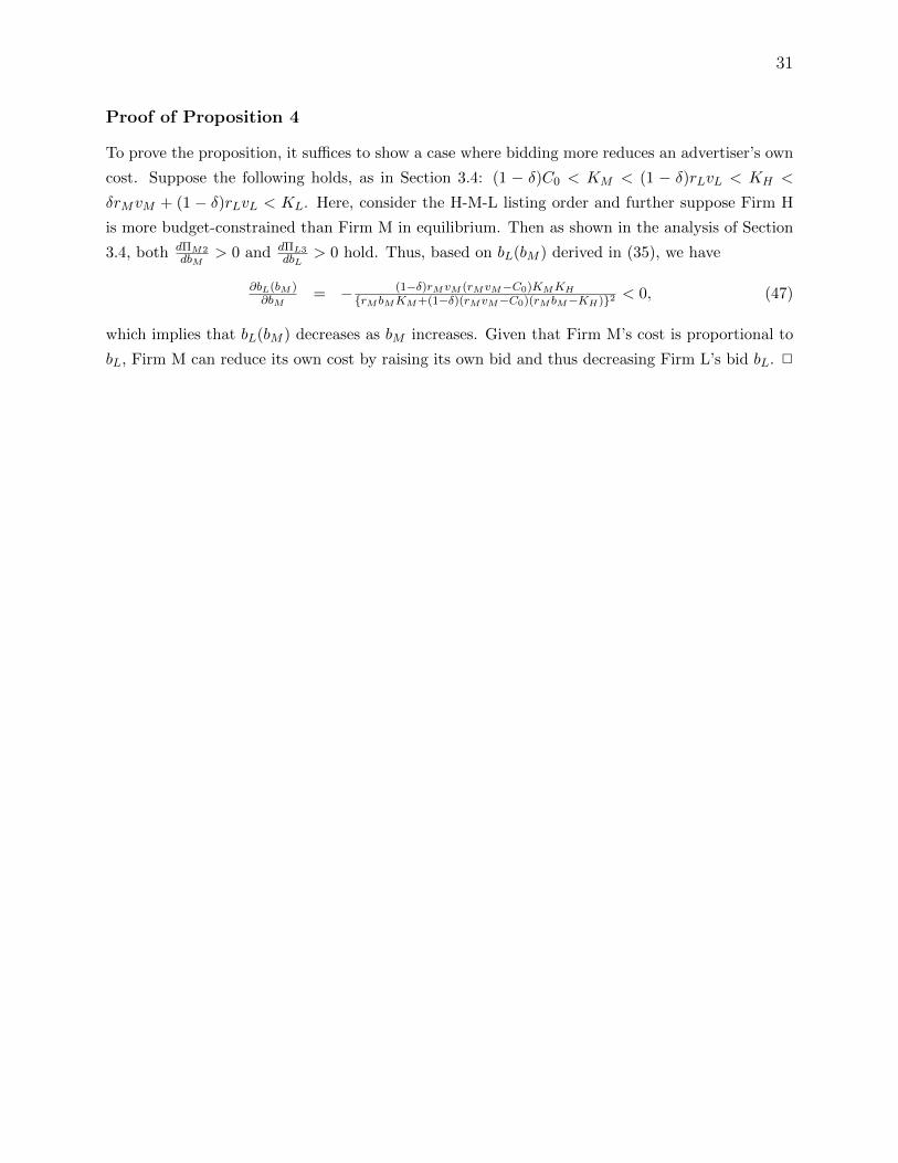
31
Proof of Proposition 4
To prove the proposition, it suffices to show a case where bidding more reduces an advertiser’s own
cost. Suppose the following holds, as in Section 3.4: (1 − δ)C0 < KM < (1 − δ)rLvL < KH <
δrMvM + (1 − δ)rLvL < KL. Here, consider the H-M-L listing order and further suppose Firm H
is more budget-constrained than Firm M in equilibrium. Then as shown in the analysis of Section
3.4, both dΠM2dbM
> 0 and dΠL3dbL
> 0 hold. Thus, based on bL(bM ) derived in (35), we have
∂bL(bM )∂bM
= − (1−δ)rMvM (rMvM−C0)KMKH{rM bMKM+(1−δ)(rMvM−C0)(rM bM−KH)}2 < 0, (47)
which implies that bL(bM ) decreases as bM increases. Given that Firm M’s cost is proportional to
bL, Firm M can reduce its own cost by raising its own bid and thus decreasing Firm L’s bid bL. 2