Keysight Technologies 10 Hints for Making Successful Noise Figure Measurements

Application Note

Optimize Your Measurements and Minimize the Uncertainties

Introduction

The checklist in Appendix A is a helpful tool to

verify that all hints have been considered

for a particular measurement.

Noise figure is often the key to characterizing a receiver and its ability to detect weak incoming signals in the presence of self-generated noise. The process of reducing noise figure begins with a solid understanding of the uncertainties in your components, subsystems and test setups. Quantifying those unknowns depends on flexible tools that provide accurate, reliable results.

Keysight Technologies, Inc. noise figure solution set—instruments, applications and accessories—helps you optimize test setups and identify unwanted sources of noise. We’ve been providing noise-figure test solutions for more than 50 years, beginning with basic noise meters and evolving into solutions based on spectrum, network, and noise-figure analyzers.

The 10 hints presented here will help minimize the uncertainties in your noise figure measurements—whether you are designing for good, better or best performance in your device. Key topics include minimizing extraneous signals, mismatch uncertainties, nonlinearities, and path losses.

3

Introduction ................................................................................................ 2HINT 1: Select the Appropriate Noise Source .................................... 4HINT 2: Minimize Extraneous Signals ................................................. 5HINT 3: Minimize Mismatch Uncertainties ......................................... 6HINT 4: Use Averaging to Minimize Display Jitter ............................ 7HINT 5: Avoid Non-Linearities .............................................................. 8HINT 6: Account for Mixer Characteristics ......................................... 9HINT 7: Use Proper Measurement Correction ................................. 12HINT 8: Choose the Optimal Measurement Bandwidth ................. 13HINT 9: Account for Path Losses ....................................................... 14HINT 10: Account for the Temperature of the Measurement Components ............................................................................................. 15Appendix A: Checklist ........................................................................... 16Appendix B: Total Uncertainty Calculations ..................................... 17Appendix C: Abbreviations ................................................................... 18Appendix D: Glossary and Definitions ............................................... 18Additional Resources ............................................................................. 19

Table of Contents

Find out more www.keysight.com/find/noisefigure

4

ENRThe output of a noise source is defined in terms of its frequency range and excess noise ratio (ENR). Nominal ENR values of 15 dB and 6 dB are commonly available. ENR values are calibrated at specific spot frequencies.

Use a 15 dB ENR noise source for: – General-purpose applications to

measure noise figure up to 30 dB.

– User-calibrating the fullest dynamic range of an instrument (before measuring high-gain devices)

Use a 6 dB ENR noise source when: – Measuring a device with gain that

is especially sensitive to changes in the source impedance

– The device under test (DUT) has a very low noise figure

– The device’s noise figure does not exceed 15 dB

A low ENR noise source will minimize error due to noise detector non-linearity. This error will be smaller if the measurement is made over a smaller, and therefore more linear, range of the instrument’s detector. A 6 dB noise source uses a smaller detector range than a 15 dB source.

A low ENR noise source will require the instrument to use the least inter-nal attenuation to cover the dynamic range of the measurement, unless the gain of the DUT is very high. Using less attenuators will lower the noise figure of the measurement instrument, which will lower the uncertainty of the measurement.

Figure 1-1. Automatic download of ENR data to the instrument speeds up overall set-up time

HINT 1: Select the Appropriate Noise Source

Frequency range Commercial noise sources cover frequencies up to 50 GHz with choices of co-axial or waveguide connectors. The frequency range of the noise source must include the input frequency range of the DUT, of course. If the DUT is a mixer or frequency translation device, the output frequency range of the DUT must also be addressed. If one source does not include both frequency ranges, a second source will be required. A second noise source may also be necessary when measuring a non-frequency translating device with low noise and high gain. Low ENR is best for the measurement, however, high ENR is necessary to calibrate the full dynamic range of the instrument. In either case, a full-featured noise figure analyzer can account for the different ENR tables required for calibration and measurement.

Match If possible, use a noise source with the lowest change in output impedance between its ON and OFF states. The noise source’s output impedance changes between its ON and OFF states, which varies the match between the noise source and the DUT. This variation changes the gain and noise figure of the DUT, especially for active devices like GaAs FET amplifiers. To minimize this effect, 6 dB ENR noise sources are commercially available that limit their changes in reflection coefficient between ON and OFF states to better than 0.01 at frequencies to 18 GHz.

Adapters Use a noise source with the cor-rect connector for the DUT rather than use an adapter, particularly for devices with gain. The ENR values for a noise source apply only at its connector. An adapter adds losses to these ENR values. The uncertainty of these losses increases the overall uncertainty of the measurement. If an adapter must be used, account for the adapter losses.

5

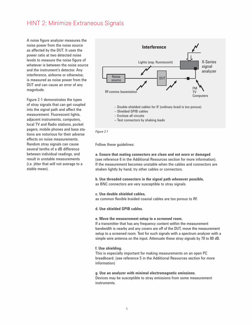
A noise figure analyzer measures the noise power from the noise source as affected by the DUT. It uses the power ratio at two detected noise levels to measure the noise figure of whatever is between the noise source and the instrument’s detector. Any interference, airborne or otherwise, is measured as noise power from the DUT and can cause an error of any magnitude.

Figure 2-1 demonstrates the types of stray signals that can get coupled into the signal path and affect the measurement. Fluorescent lights, adjacent instruments, computers, local TV and Radio stations, pocket pagers, mobile phones and base sta-tions are notorious for their adverse effects on noise measurements. Random stray signals can cause several tenths of a dB difference between individual readings, and result in unstable measurements (i.e. jitter that will not average to a stable mean).

Interference

Noisesource

Lights (esp. fluorescent)

FMTVComputers

– Double-shielded cables for IF (ordinary braid is too porous)– Shielded GPIB cables– Enclose all circuits– Test connectors by shaking leads

X-Seriessignalanalyzer

RF comms basestation

DUT

Figure 2-1

HINT 2: Minimize Extraneous Signals

Follow these guidelines:

a. Ensure that mating connectors are clean and not worn or damaged (see reference 6 in the Additional Resources section for more information). If the measurement becomes unstable when the cables and connectors are shaken lightly by hand, try other cables or connectors.

b. Use threaded connectors in the signal path whenever possible, as BNC connectors are very susceptible to stray signals.

c. Use double shielded cables, as common flexible braided coaxial cables are too porous to RF.

d. Use shielded GPIB cables.

e. Move the measurement setup to a screened room. If a transmitter that has any frequency content within the measurement bandwidth is nearby and any covers are off of the DUT, move the measurement setup to a screened room. Test for such signals with a spectrum analyzer with a simple wire antenna on the input. Attenuate these stray signals by 70 to 80 dB.

f. Use shielding. This is especially important for making measurements on an open PC breadboard. (see reference 5 in the Additional Resources section for more information)

g. Use an analyzer with minimal electromagnetic emissions. Devices may be susceptible to stray emissions from some measurement instruments.

6

Figure 3-1

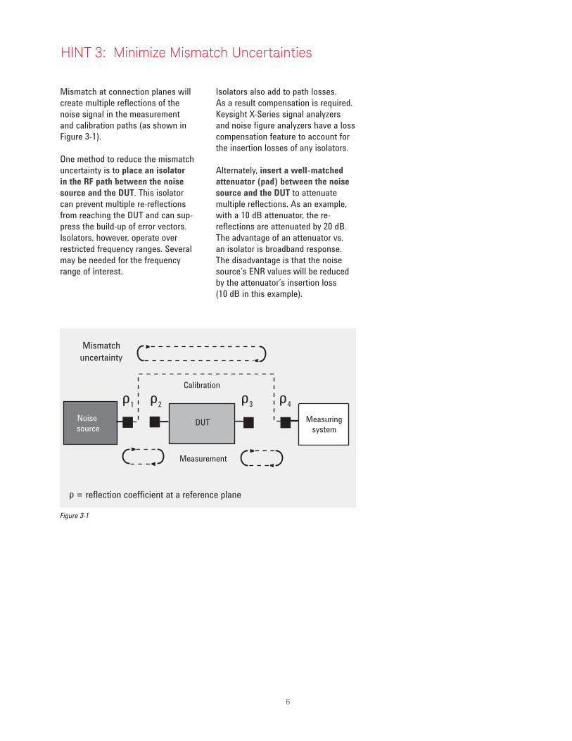
Mismatch at connection planes will create multiple reflections of the noise signal in the measurement and calibration paths (as shown in Figure 3-1).

One method to reduce the mismatch uncertainty is to place an isolator in the RF path between the noise source and the DUT. This isolator can prevent multiple re-reflections from reaching the DUT and can sup-press the build-up of error vectors. Isolators, however, operate over restricted frequency ranges. Several may be needed for the frequency range of interest.

Isolators also add to path losses. As a result compensation is required. Keysight X-Series signal analyzers and noise figure analyzers have a loss compensation feature to account for the insertion losses of any isolators.

Alternately, insert a well-matched attenuator (pad) between the noise source and the DUT to attenuate multiple reflections. As an example, with a 10 dB attenuator, the re-reflections are attenuated by 20 dB. The advantage of an attenuator vs. an isolator is broadband response. The disadvantage is that the noise source’s ENR values will be reduced by the attenuator’s insertion loss (10 dB in this example).

Measuringsystem

Noise source DUT

Calibration

Measurement

Mismatchuncertainty

ρ1 ρ2 ρ4ρ3

ρ = reflection coefficient at a reference plane

HINT 3: Minimize Mismatch Uncertainties

7

Mismatch at connection planes with noise measurement inherently displays variability or jitter because of the random nature of the noise being measured. Averaging many readings can minimize displayed jitter and bring the measurement closer to the true mean of the noise’s Gaussian distribution.

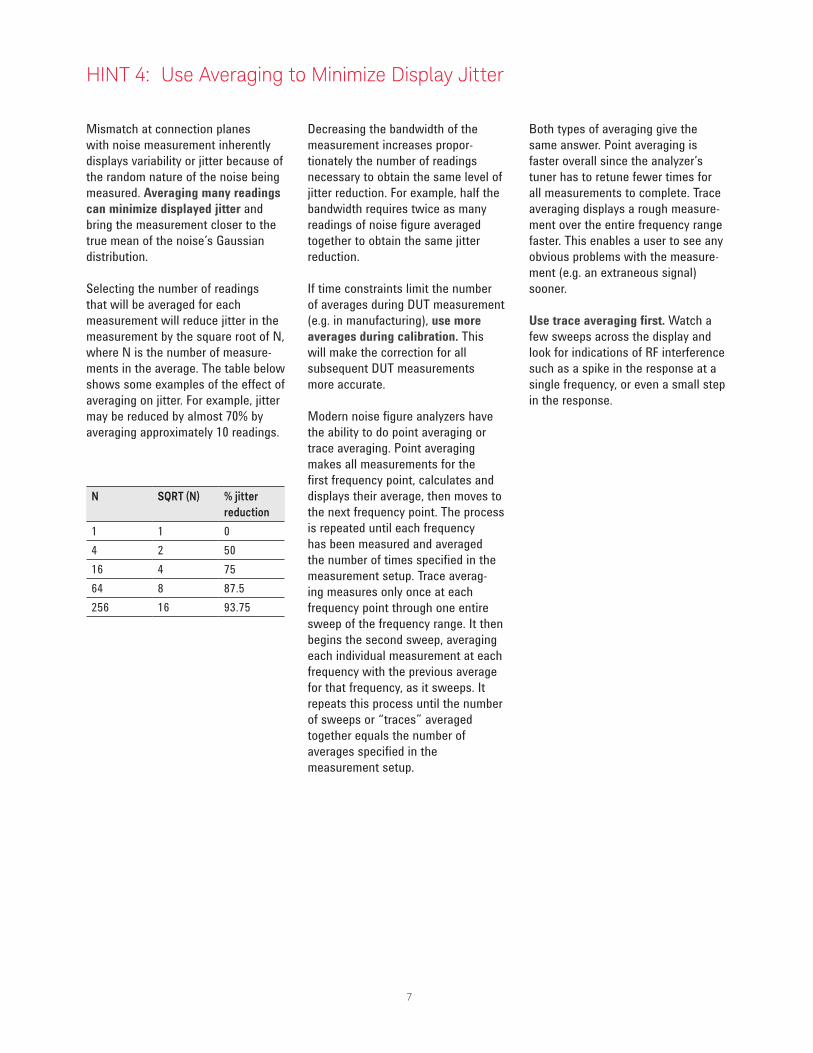
Selecting the number of readings that will be averaged for each measurement will reduce jitter in the measurement by the square root of N, where N is the number of measure-ments in the average. The table below shows some examples of the effect of averaging on jitter. For example, jitter may be reduced by almost 70% by averaging approximately 10 readings.

Decreasing the bandwidth of the measurement increases propor-tionately the number of readings necessary to obtain the same level of jitter reduction. For example, half the bandwidth requires twice as many readings of noise figure averaged together to obtain the same jitter reduction.

If time constraints limit the number of averages during DUT measurement (e.g. in manufacturing), use more averages during calibration. This will make the correction for all subsequent DUT measurements more accurate.

Modern noise figure analyzers have the ability to do point averaging or trace averaging. Point averaging makes all measurements for the first frequency point, calculates and displays their average, then moves to the next frequency point. The process is repeated until each frequency has been measured and averaged the number of times specified in the measurement setup. Trace averag-ing measures only once at each frequency point through one entire sweep of the frequency range. It then begins the second sweep, averaging each individual measurement at each frequency with the previous average for that frequency, as it sweeps. It repeats this process until the number of sweeps or “traces” averaged together equals the number of averages specified in the measurement setup.

Both types of averaging give the same answer. Point averaging is faster overall since the analyzer’s tuner has to retune fewer times for all measurements to complete. Trace averaging displays a rough measure-ment over the entire frequency range faster. This enables a user to see any obvious problems with the measure-ment (e.g. an extraneous signal) sooner.

Use trace averaging first. Watch a few sweeps across the display and look for indications of RF interference such as a spike in the response at a single frequency, or even a small step in the response.

N SQRT (N) % jitter reduction

1 1 04 2 5016 4 7564 8 87.5256 16 93.75

HINT 4: Use Averaging to Minimize Display Jitter

8

Avoid all predictable sources of nonlinearities:

– Circuits with phase lock loops (and any circuit that relies on signal presence to set its operating condition)

– Circuits that oscillate (even if at a far-removed frequency)

– Amplifiers or mixers that are operating near saturation

– AGC circuits or limiters (AGC circuits have been known to contribute additional noise power at the power levels near its operational point, even when disabled.)

– High-gain DUTs without in-line attenuation (Attenuate the output of the DUT if necessary. See Hint 7 for details)

– Power supply drifts

– DUTs or measurement systems that have not warmed up

– Logarithmic amplifiers (The standard Y-factor measurement is invalid for amplifiers in a logarithmic mode.)

Hint 5: Avoid Nonlinearities

A Y-factor noise figure analyzer assumes a linear change in the detected noise power as the noise source is switched between Thot and Tcold. Any variations from linearity in either the DUT or in the detector directly produce an error in the Y value and hence in the noise figure that is displayed. The instrumentation uncertainty specification accounts for the linearity of the analyzer’s detector. The linearity of the DUT, however, should be carefully considered when making the measurement.

The measured noise figure is determined by the power in the instrument’s resolution bandwidth. The instrument’s attenuation settings, however, may be determined by the power in the instrument’s overall fre-quency range that reaches the range detector. The analyzer is therefore susceptible to being overdriven by noise outside the bandwidth of any one individual measurement, and therefore vulnerable to non-linearity errors. In such cases, attenuate any broadband power outside the ana-lyzer’s resolution bandwidth. Use a filter wider than the measurement frequency range and before the DUT.

Consider measuring a familiar “ reference” or “gold standard” device at the beginning of each day to assure that the same result is obtained as prior days for the same device, to add assurance that the measurement instrument is warmed up sufficiently.

9

Figure 6-1

If the device under test is a mixer:

– Measure the same sideband(s) that will be used in the application of the mixer.

– For double sideband measurements, select a LO frequency close to the RF band of interest.

– For single sideband measurements, select a LO far from the RF band of interest, if possible.

– Choose the LO to suit the mixer.

– Filter the RF signal (i.e. the noise source) if necessary to remove unwanted signals that would mix with the LO’s harmonics or spurious signals.

– Always document a frequency plan to identify which of the above precautions are necessary.

Noise

pow

erFreq

LSB

USB

FLO

FIF

Average

HINT 6: Account for Mixer Characteristics

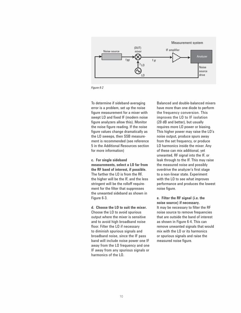
a. Select a double sideband or a single sideband measurement.A mixer will translate input signals and noise from the upper sideband (USB) and lower sideband (LSB) as Figure 6-1 shows. (Note that the LSB and USB are separated by twice the IF.) A double sideband (DSB) measurement, shown in Figure 6-2, measures the noise powers for both the USB and LSB. Some receiver sys-tems, like those in radio astronomy, intentionally use both sidebands. DSB noise figure measurement is appropriate in these cases. In many applications the desired signal will be seen in only one sideband. A single sideband (SSB) measurement is appropriate in these cases. In SSB measurement setups, the noise power in the unwanted sideband is suppressed by appropriate “image rejection” filtering at the input of the mixer.

DSB measurements are easier to perform since they don’t require the additional burden of image rejection filter design and matching. When a mixer with a DSB specified noise figure is going to be used in an SSB application, careful correction is needed. (see reference 5 in the Additional Resources section for more information)

b. For double sideband measurements, select a LO frequency as close as possible to the RF band of interest. The choice of LO frequency, and the resulting IF, can make a dramatic difference in the results of DSB mea-surements. Instruments typically display the average of the LSB and USB noise figures. They measure the power in the IF band (which is the sum of both sidebands after conver-sion), diminish that power by half (3 dB), and display the result. The closer the USB and LSB are together, the more likely they are to be equal (as shown in Figure 6-1) and the more likely the default 3 dB correction will be accurate. Since noise power versus frequency for a mixer is rarely flat, if too wide an IF is used the error and its correction will be unknown. To minimize this error, choose the LO frequency as close as possible to the RF band of interest, within the limita-tion that the resulting IF cannot be below the lower frequency limit of the instrument being used (often 10 MHz).

10

To determine if sideband-averaging error is a problem, set up the noise figure measurement for a mixer with swept LO and fixed IF (modern noise figure analyzers allow this). Monitor the noise figure reading. If the noise figure values change dramatically as the LO sweeps, then SSB measure-ment is recommended (see reference 5 in the Additional Resources section for more information)

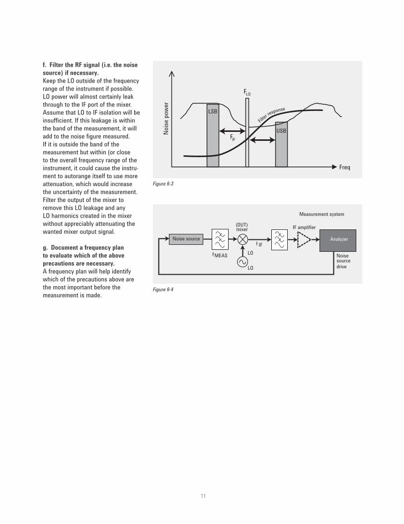
c. For single sideband measurements, select a LO far from the RF band of interest, if possible. The farther the LO is from the RF, the higher will be the IF, and the less stringent will be the rolloff require-ment for the filter that suppresses the unwanted sideband as shown in Figure 6-3.

d. Choose the LO to suit the mixer.Choose the LO to avoid spurious output where the mixer is sensitive and to avoid high broadband noise floor. Filter the LO if necessary to diminish spurious signals and broadband noise, since the IF pass band will include noise power one IF away from the LO frequency and one IF away from any spurious signals or harmonics of the LO.

Balanced and double-balanced mixers have more than one diode to perform the frequency conversion. This improves the LO to IF isolation (20 dB and better), but usually requires more LO power or biasing. This higher power may raise the LO’s noise output, produce spurs away from the set frequency, or produce LO harmonics inside the mixer. Any of these can mix additional, yet unwanted, RF signal into the IF, or leak through to the IF. This may raise the measured noise and possibly overdrive the analyzer’s first stage to a non-linear state. Experiment with the LO to see what improves performance and produces the lowest noise figure.

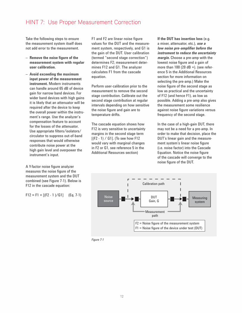
e. Filter the RF signal (i.e. the noise source) if necessary. It may be necessary to filter the RF noise source to remove frequencies that are outside the band of interest as shown in Figure 6-4. This can remove unwanted signals that would mix with the LO or its harmonics or spurious signals and raise the measured noise figure.

Noise source IF amplifiermixer

fLO

IFfRF

LO

Measurement system

Noise source drive

(DUT)

f

Analyzer

Figure 6-2

11

Noise

pow

erFreq

LSB

USB

FLO

FIF

Filter r

esponse

Analyzer

IF amplifiermixer

fLO

IF

fMEAS

LO

Measurement system

Noisesourcedrive

(DUT)

Noise source

Figure 6-3

Figure 6-4

f. Filter the RF signal (i.e. the noise source) if necessary. Keep the LO outside of the frequency range of the instrument if possible. LO power will almost certainly leak through to the IF port of the mixer. Assume that LO to IF isolation will be insufficient. If this leakage is within the band of the measurement, it will add to the noise figure measured. If it is outside the band of the measurement but within (or close to the overall frequency range of the instrument, it could cause the instru-ment to autorange itself to use more attenuation, which would increase the uncertainty of the measurement. Filter the output of the mixer to remove this LO leakage and any LO harmonics created in the mixer without appreciably attenuating the wanted mixer output signal.

g. Document a frequency plan to evaluate which of the above precautions are necessary. A frequency plan will help identify which of the precautions above are the most important before the measurement is made.

12

Figure 7-1

Take the following steps to ensure the measurement system itself does not add error to the measurement.

– Remove the noise figure of the measurement system with regular user calibration.

– Avoid exceeding the maximum input power of the measurement instrument. Modern instruments can handle around 65 dB of device gain for narrow band devices. For wider band devices with high gains it is likely that an attenuator will be required after the device to keep the overall power within the instru-ment’s range. Use the analyzer’s compensation feature to account for the losses of the attenuator. Use appropriate filters/isolators/circulator to suppress out-of-band responses that would otherwise contribute noise power at the high gain level and overpower the instrument’s input.

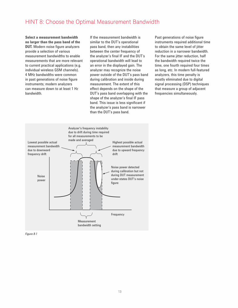
A Y-factor noise figure analyzer measures the noise figure of the measurement system and the DUT combined (see Figure 7-1). Below is F12 in the cascade equation:

F12 = F1 + [(F2 - 1 )/G1] (Eq. 7-1)

F1 and F2 are linear noise figure values for the DUT and the measure-ment system, respectively, and G1 is the gain of the DUT. User calibration (termed “second stage correction”) determines F2; measurement deter-mines F12 and G1. The analyzer calculates F1 from the cascade equation.

Perform user-calibration prior to the measurement to remove the second stage contribution. Calibrate out the second stage contribution at regular intervals depending on how sensitive the noise figure and gain are to temperature drifts.

The cascade equation shows how F12 is very sensitive to uncertainty margins in the second stage term [(F2 - 1) / G1]. (To see how F12 would vary with marginal changes in F2 or G1, see reference 5 in the Additional Resources section)

If the DUT has insertion loss (e.g. a mixer, attenuator, etc.), use a low noise pre-amplifier before the instrument to reduce the uncertainty margin. Choose a pre-amp with the lowest noise figure and a gain of more than 100 (20 dB +). (see refer-ence 5 in the Additional Resources section for more information on selecting the pre-amp.) Make the noise figure of the second stage as low as practical and the uncertainty of F12 (and hence F1), as low as possible. Adding a pre-amp also gives the measurement some resilience against noise figure variations versus frequency of the second stage.

In the case of a high-gain DUT, there may not be a need for a pre-amp. In order to make that decision, place the DUT’s linear gain and the measure-ment system’s linear noise figure (i.e. noise factor) into the Cascade Equation. Notice the noise figure of the cascade will converge to the noise figure of the DUT.

Noisesource

Measuringsystem

DUTGain, G

Calibration path

Measurementpath

F2 = Noise figure of the measurement systemF1 = Noise figure of the device under test (DUT)

HINT 7: Use Proper Measurement Correction

13

Figure 8-1

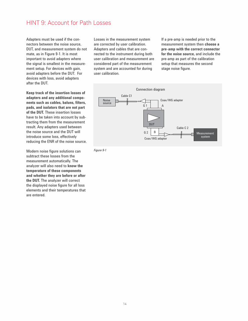
Select a measurement bandwidth no larger than the pass band of the DUT. Modern noise figure analyzers provide a selection of various measurement bandwidths to enable measurements that are more relevant to current practical applications (e.g. individual wireless GSM channels). 4 MHz bandwidths were common in past generations of noise figure instruments; modern analyzers can measure down to at least 1 Hz bandwidth.

If the measurement bandwidth is similar to the DUT’s operational pass band, then any instabilities between the center frequency of the analyzer’s final IF and the DUT’s operational bandwidth will lead to an error in the displayed gain. The analyzer may recognize the noise power outside of the DUT’s pass band during calibration and inside during measurement. The extent of this effect depends on the shape of the DUT’s pass band overlapping with the shape of the analyzer’s final IF pass band. This issue is less significant if the analyzer’s pass band is narrower than the DUT’s pass band.

Past generations of noise figure instruments required additional time to obtain the same level of jitter reduction in a narrower bandwidth. For the same jitter reduction, half the bandwidth required twice the time, one fourth required four times as long, etc. In modern full-featured analyzers, this time penalty is mostly eliminated due to digital signal processing (DSP) techniques that measure a group of adjacent frequencies simultaneously.

Frequency

Measurementbandwidth setting

Noise power detected during calibration but not during DUT measurement under-states DUT's noise figure

Noisepower

Lowest possible actualmeasurement bandwidth due to downward frequency drift

Analyzer's frequency instability due to drift during time required for all measurements to be made and averaged Highest possible actual

measurement bandwidth due to upward frequency drift

HINT 8: Choose the Optimal Measurement Bandwidth

14

Adapters must be used if the con-nectors between the noise source, DUT, and measurement system do not mate, as in Figure 9-1. It is most important to avoid adapters where the signal is smallest in the measure-ment setup. For devices with gain, avoid adapters before the DUT. For devices with loss, avoid adapters after the DUT.

Keep track of the insertion losses of adapters and any additional compo-nents such as cables, baluns, filters, pads, and isolators that are not part of the DUT. These insertion losses have to be taken into account by sub-tracting them from the measurement result. Any adapters used between the noise source and the DUT will introduce some loss, effectively reducing the ENR of the noise source.

Modern noise figure solutions can subtract these losses from the measurement automatically. The analyzer will also need to know the temperature of these components and whether they are before or after the DUT. The analyzer will correct the displayed noise figure for all loss elements and their temperatures that are entered.

Losses in the measurement system are corrected by user calibration. Adapters and cables that are con-nected to the instrument during both user calibration and measurement are considered part of the measurement system and are accounted for during user calibration.

If a pre-amp is needed prior to the measurement system then choose a pre-amp with the correct connector for the noise source, and include the pre-amp as part of the calibration setup that measures the second stage noise figure.

Figure 9-1

Connection diagram

Noisesource

DUT

Measurementsystem

G 1

G 2

Cable C1

Cable C 2

Coax/WG adapter

Coax/WG adapter

A

B

HINT 9: Account for Path Losses

15

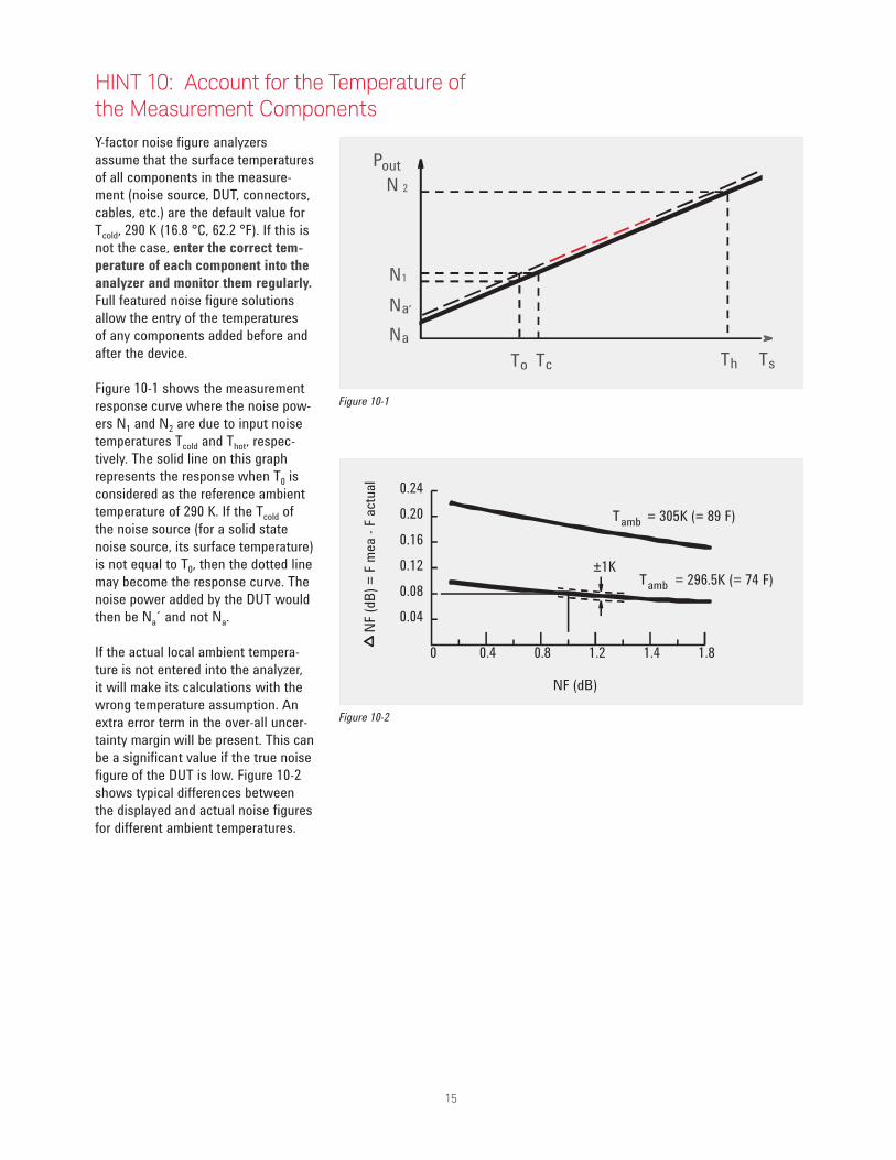
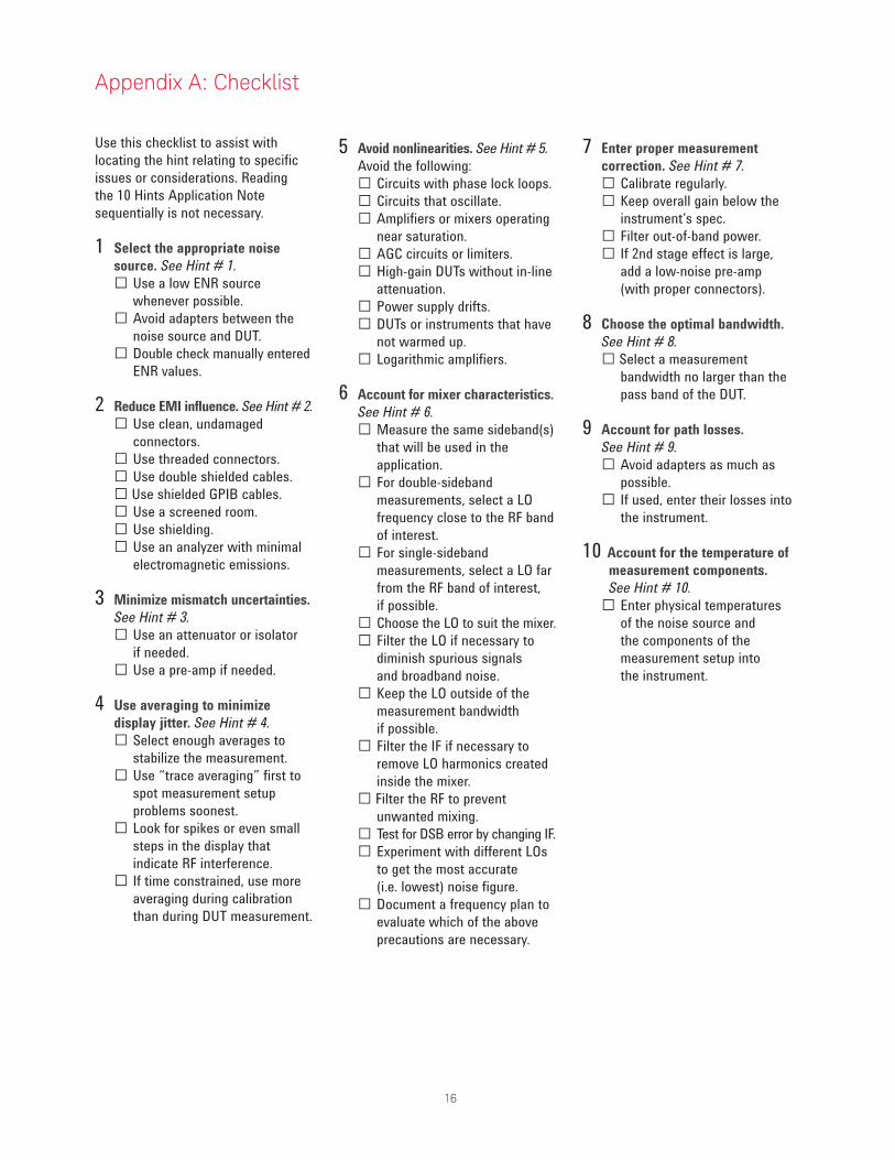
Y-factor noise figure analyzers assume that the surface temperatures of all components in the measure-ment (noise source, DUT, connectors, cables, etc.) are the default value for Tcold, 290 K (16.8 °C, 62.2 °F). If this is not the case, enter the correct tem-perature of each component into the analyzer and monitor them regularly. Full featured noise figure solutions allow the entry of the temperatures of any components added before and after the device.

Figure 10-1 shows the measurement response curve where the noise pow-ers N1 and N2 are due to input noise temperatures Tcold and Thot, respec-tively. The solid line on this graph represents the response when T0 is considered as the reference ambient temperature of 290 K. If the Tcold of the noise source (for a solid state noise source, its surface temperature) is not equal to T0, then the dotted line may become the response curve. The noise power added by the DUT would then be Na´ and not Na.

If the actual local ambient tempera-ture is not entered into the analyzer, it will make its calculations with the wrong temperature assumption. An extra error term in the over-all uncer-tainty margin will be present. This can be a significant value if the true noise figure of the DUT is low. Figure 10-2 shows typical differences between the displayed and actual noise figures for different ambient temperatures.

PoutN 2

N1

Na

NaTo Tc Th Ts

±1KT amb = 296.5K (= 74 F)

T amb = 305K (= 89 F)

0.240.20

0.160.120.080.04

0 0.4 0.8 1.2 1.4 1.8

NF (dB)

NF (d

B) =

F m

ea -

F act

ual

Figure 10-1

Figure 10-2

HINT 10: Account for the Temperature of the Measurement Components

16

Use this checklist to assist with locating the hint relating to specific issues or considerations. Reading the 10 Hints Application Note sequentially is not necessary. 1 Select the appropriate noise source. See Hint # 1. □ Use a low ENR source whenever possible. □ Avoid adapters between the noise source and DUT. □ Double check manually entered ENR values.

2 Reduce EMI influence. See Hint # 2. □ Use clean, undamaged connectors. □ Use threaded connectors. □ Use double shielded cables. □ Use shielded GPIB cables. □ Use a screened room. □ Use shielding. □ Use an analyzer with minimal electromagnetic emissions.

3 Minimize mismatch uncertainties. See Hint # 3. □ Use an attenuator or isolator if needed. □ Use a pre-amp if needed.

4 Use averaging to minimize display jitter. See Hint # 4. □ Select enough averages to stabilize the measurement. □ Use “trace averaging” first to spot measurement setup problems soonest. □ Look for spikes or even small steps in the display that indicate RF interference. □ If time constrained, use more averaging during calibration than during DUT measurement.

Appendix A: Checklist

5 Avoid nonlinearities. See Hint # 5. Avoid the following: □ Circuits with phase lock loops. □ Circuits that oscillate. □ Amplifiers or mixers operating near saturation. □ AGC circuits or limiters. □ High-gain DUTs without in-line attenuation. □ Power supply drifts. □ DUTs or instruments that have not warmed up. □ Logarithmic amplifiers.

6 Account for mixer characteristics. See Hint # 6. □ Measure the same sideband(s) that will be used in the application. □ For double-sideband measurements, select a LO frequency close to the RF band of interest. □ For single-sideband measurements, select a LO far from the RF band of interest, if possible. □ Choose the LO to suit the mixer. □ Filter the LO if necessary to diminish spurious signals and broadband noise. □ Keep the LO outside of the measurement bandwidth if possible. □ Filter the IF if necessary to remove LO harmonics created inside the mixer. □ Filter the RF to prevent unwanted mixing. □ Test for DSB error by changing IF. □ Experiment with different LOs to get the most accurate (i.e. lowest) noise figure. □ Document a frequency plan to evaluate which of the above precautions are necessary.

7 Enter proper measurement correction. See Hint # 7. □ Calibrate regularly. □ Keep overall gain below the instrument’s spec. □ Filter out-of-band power. □ If 2nd stage effect is large, add a low-noise pre-amp (with proper connectors).

8 Choose the optimal bandwidth. See Hint # 8. □ Select a measurement bandwidth no larger than the pass band of the DUT.

9 Account for path losses. See Hint # 9. □ Avoid adapters as much as possible. □ If used, enter their losses into the instrument.

10 Account for the temperature of measurement components. See Hint # 10. □ Enter physical temperatures of the noise source and the components of the measurement setup into the instrument.

17

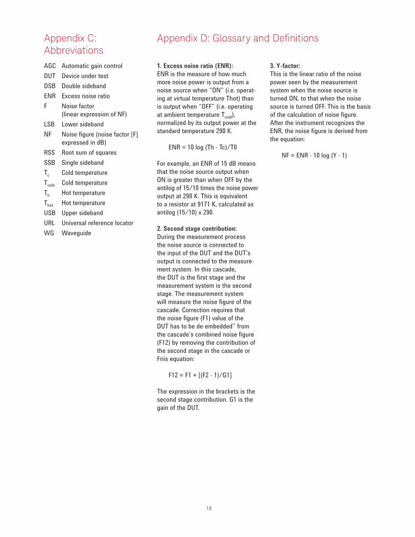
The error model in the spreadsheet shown in Figure B-1 is obtained from the derivative of the Cascade equation (F1 = F12 - [(F2-1)/G1]). It takes into account the individual mismatch uncertainty calculations at each reference or incident plane of the DUT, noise source and measurement system. This example represents the total noise figure measurement uncertainty, RSS analysis, for a microwave transistor with an S11 of 0.5, S22 of 0.8 and S21 of 5 (14 dB). Noise figure uncertainty, here is cal-culated as ±0.48 dB. The uncertainty dramatically improves to ±0.26 dB, in this instance, if the gain is improved to 20 dB. The calculation for this error model is derived from reference 5 in the Additional Resources section.

Figure B-2

Figure B-4

Figure B-3

Figure B-1

Figure B-5

Appendix B: Total Uncertainty Calculations

Figure B-2 shows the typical display for the entry point to this interactive model. Figures B-3, B-4 and B-5 show simulated results for the uncertainty calculator. There are a number of graphs that can be plotted. These figures show examples of RSS uncertainty with respect to instrument match,

DUT input match and instrument noise figure, respectively. This inter-active uncertainty calculator and the spreadsheet version shown in Figure B-1 can be accessed via the Internet by using the URL on the back page of this application note.

18

AGC Automatic gain control DUT Device under test DSB Double sideband ENR Excess noise ratio F Noise factor (linear expression of NF) LSB Lower sideband NF Noise figure (noise factor [F] expressed in dB) RSS Root sum of squares SSB Single sideband Tc Cold temperature Tcold Cold temperature Th Hot temperature Thot Hot temperature USB Upper sideband URL Universal reference locatorWG Waveguide

1. Excess noise ratio (ENR): ENR is the measure of how much more noise power is output from a noise source when “ON” (i.e. operat-ing at virtual temperature Thot) than is output when “OFF” (i.e. operating at ambient temperature Tcold), normalized by its output power at the standard temperature 290 K.

ENR = 10 log (Th - Tc)/T0

For example, an ENR of 15 dB means that the noise source output when ON is greater than when OFF by the antilog of 15/10 times the noise power output at 290 K. This is equivalent to a resistor at 9171 K, calculated as antilog (15/10) x 290.

2. Second stage contribution: During the measurement process the noise source is connected to the input of the DUT and the DUT’s output is connected to the measure-ment system. In this cascade, the DUT is the first stage and the measurement system is the second stage. The measurement system will measure the noise figure of the cascade. Correction requires that the noise figure (F1) value of the DUT has to be de-embedded” from the cascade’s combined noise figure (F12) by removing the contribution of the second stage in the cascade or Friis equation:

F12 = F1 + [(F2 - 1)/G1]

The expression in the brackets is the second stage contribution. G1 is the gain of the DUT.

Appendix C: Abbreviations

Appendix D: Glossary and Definitions

3. Y-factor: This is the linear ratio of the noise power seen by the measurement system when the noise source is turned ON, to that when the noise source is turned OFF. This is the basis of the calculation of noise figure. After the instrument recognizes the ENR, the noise figure is derived from the equation:

NF = ENR - 10 log (Y - 1)

19

For more information on noise figure and Keysight Technologies’ noise figure solutions, see below.

Noise figure solutions:1. www.keysight.com/find/noisefigure

2. Hints for Making Better Noise Figure Measurements – video series: www.keysight.com/find/noisefigurevideos

3. Noise Figure Selection Guide, literature number 5989-8056EN

4. Fundamentals of Noise Figure Measurements (AN 57-1), Application Note, literature number 5952-8255E

5. Noise Figure Measurement Accuracy (AN 57-2), Application Note, literature number 5952-3706E

6. Principles of Microwave Connector Care, Application Note, literature number 5954-1566

Additional Resources

This information is subject to change without notice.© Keysight Technologies, 2011 - 2014Published in USA, August 1, 20145980-0288Ewww.keysight.com

20 | Keysight | 10 Hints for Making Successful Noise Figure Measurements - Application Note

For more information on Keysight Technologies’ products, applications or services, please contact your local Keysight office. The complete list is available at:www.keysight.com/find/contactus

Americas Canada (877) 894 4414Brazil 55 11 3351 7010Mexico 001 800 254 2440United States (800) 829 4444

Asia PacificAustralia 1 800 629 485China 800 810 0189Hong Kong 800 938 693India 1 800 112 929Japan 0120 (421) 345Korea 080 769 0800Malaysia 1 800 888 848Singapore 1 800 375 8100Taiwan 0800 047 866Other AP Countries (65) 6375 8100

Europe & Middle EastAustria 0800 001122Belgium 0800 58580Finland 0800 523252France 0805 980333Germany 0800 6270999Ireland 1800 832700Israel 1 809 343051Italy 800 599100Luxembourg +32 800 58580Netherlands 0800 0233200Russia 8800 5009286Spain 0800 000154Sweden 0200 882255Switzerland 0800 805353

Opt. 1 (DE)Opt. 2 (FR)Opt. 3 (IT)

United Kingdom 0800 0260637

For other unlisted countries:www.keysight.com/find/contactus(BP-05-23-14)

myKeysight

www.keysight.com/find/mykeysightA personalized view into the information most relevant to you.

www.lxistandard.org

LAN eXtensions for Instruments puts the power of Ethernet and the Web inside your test systems. Keysight is a founding member of the LXI consortium.

Three-Year Warranty

www.keysight.com/find/ThreeYearWarrantyKeysight’s commitment to superior product quality and lower total cost of ownership. The only test and measurement company with three-year warranty standard on all instruments, worldwide.

Keysight Assurance Planswww.keysight.com/find/AssurancePlansUp to five years of protection and no budgetary surprises to ensure your instruments are operating to specification so you can rely on accurate measurements.

www.keysight.com/qualityKeysight Electronic Measurement GroupDEKRA Certified ISO 9001:2008 Quality Management System

Keysight Channel Partnerswww.keysight.com/find/channelpartnersGet the best of both worlds: Keysight’s measurement expertise and product breadth, combined with channel partner convenience.

www.keysight.com/find/noisefigure