Kernel Techniques for Generalized AudioCrossfades

William A. Sethares and James A. Bucklew∗

July 10, 2015

Abstract

This paper explores a variety of density and kernel-based techniques thatcan smoothly connect (crossfade or “morph” between) two functions. Whenthe functions represent audio spectra, this provides a concrete way of ad-justing the partials of a sound while smoothly interpolating between exist-ing sounds. The approach can be applied to both interpolation-crossfades(where the crossfade connects two different sounds over a specified dura-tion) and to repetitive-crossfades (where a series of sounds are generated,each containing progressively more features of one sound and fewer of theother). The interpolation surface can be thought of as the two dimensions(time and frequency) of a spectrogram, and the kernels can be chosen so asto constrain the surface in a number of desirable ways. When successful, thetimbre of the sounds is changed dynamically in a plausible way. A series ofsound examples demonstrate the strengths and weaknesses of the approach.

∗Both authors are with the Department of Electrical and Computer Engineering, University ofWisconsin, Madison, USA, sethares@ece.wisc.edu and bucklew@engr.wisc.edu

1

Public Interest Statement

A common cinematic effect is the morphing of one image to another: a persontransforms smoothly into a werewolf or the features of one person change fluidlyinto those of another. The analogous effect in audition is sometimes called a cross-fade, and this paper examines two kinds of generalized crossfades that allow onesound to smoothly transform into another. Using ideas from differential equationsand probability theory, the “kernel” of the crossfade is defined, and its structurehelps to determine the behavior of the resulting sound in terms of audible ridges.A number of sound examples present the uses and limitations of the method.

About the Authors

William Sethares and James Bucklew are both with the department of Electri-cal and Computer Engineering at the University of Wisconsin-Madison. Their re-search interests include signal processing as applied to audio, images, and telecom-munications.

2

1 IntroductionCrossfading between two sounds can be simple: one sound decreases in volume asthe second sound increases in volume. More interesting crossfades may attemptto maintain common aspects of the sounds while smoothly changing dissimilaraspects. For example, it may be desirable to gradually transform one sound intoanother while requiring that nearby partials sweep between nearby partials, or itmay be advantageous to require that the sound retains its harmonic integrity overthe duration of the crossfade. Sometimes called audio morphing, such generalizedcrossfades are an area of investigation in the computer music field [16], [17] andthe techniques may also find use in speech synthesis, where smoothly connectingspeech sounds is not a trivial operation [4].

Two kinds of crossfades may be distinguished based on the information usedand the desired time over which the fade is to be conducted. In interpolation cross-fades, two sounds A and B are separated in time by some interval t. The goal ofthe fade is to smoothly and continuously change from A (the source) to B (thedestination) over the time t. The fade “fills in” the time between a single (starting)frame in A and a single (ending) frame in B. Figure 1(a) shows this schemati-cally. In a repetitive crossfade, the goal is to create a series of intermediate soundsMi, i = 1, 2, . . . n each of which exhibits progressively more aspects of B andfewer aspects of A, as shown in Fig. 1(b). Observe that repetitive crossfading isformally analogous to image morphing since it creates a series of intermediariesbetween the specified start and end points. Interpolation crossfades, by filling ina silence between two sounds, can be thought of as a time-stretching procedurewhere the start and end sounds may be chosen arbitrarily. In both cases, kernel-based techniques can be used to place constraints on and guide the crossfade.

Perhaps the most common strategy for creating audio morphings is to:

(i) derive sets of features fA and fB,

(ii) create a correspondence where features in sound A are assigned to featuresin sound B

(iii) interpolate between the corresponding features over the specified time ofthe morph

(iv) synthesize the morphed sound from the interpolated features.

Most current approaches to morphing follow the general plan (i)-(iv). For exam-ple, [1] models the sound as a Gaussian Mixture which is trained on notes from

3

source A destination B

duration of crossfadestart frame

source

destination

frames

end frame

M1

M2

Mn-1

Mn

most like source

most like destination

aspects of both

source and destination }

} }(a) interpolation crossfade

time

(b) repetitive crossfade

t

A

B

Figure 1: Audio crossfades generate sounds that change smoothly between asource and a destination sound. In interpolation crossfades (a), the sound be-gins as A and over time smoothly becomes like B. The total duration of theoutput sound is independent of the duration of A and B and the cross only de-pends on the sound in the starting and ending frames. The overall effect is oneof stretching time under the constraint that the sound must emerge continuouslyfrom A and merge continuously into B. In repetitive crossfades (b), a series ofintermediate sounds Mi merge aspects of A and B, analogous to the intermedi-ary photographs of an image morph that merges various aspects of the startingand ending photographs. The duration of each output sound Mi is equal to thecommon duration of A and B. Thus interpolation crosses begin as one sound andend as another while in a repetitive cross, each Mi contains features of both ofthe original sounds. For instance, an interpolation crossfade might start with theattack portion of a cymbal and end with the final moments of a lion’s roar. Theinterpolation crossfade is the transition that occurs over a user specified time. Incontrast, each intermediate sound in a repetitive crossfade merges aspects of boththe complete lion sound (from start to end) with those of the complete cymbal(from attack through decay).

4

the same instrument played with different intensities, or on notes from differentinstruments. Other approaches exploit the sinusoidal plus noise decompositionof Serra [13] or use the bandwidth-enhanced sinusoidal approach [5] to allow forthe more faithful reproduction of nonsinusoidal elements in the sound. A varietyof spectral manipulations including audio morphings are suggested by Erbe [3]and Polansky [12]. Our previous work [15] separated the noise part of the soundfrom the tonal part using a median filter, then morphed the two parts indepen-dently. Most such methods incorporate peak-finding routines (as may be familiarfrom McAulay and Quatieri’s tracking method [9]) in the choice of features anduse some kind of ad hoc assignment method for creating the correspondences.Tellman [17] describes some of the issues that arise when carrying out complexassignments.

This paper suggests an alternative procedure for the construction of smoothaudio connections that generalizes to any sensible kernel function. An advantageof this method is that two of the common problems in the general scheme (i)-(iv)are avoided. First, no choice of specific features is made and there is no need tolocate significant partials or features in the sound. Hence there can be no mistakesmade in identifying such features. Second, since the crossfade is defined by a PDEor, in a probabilistic sense, as a density or kernel function, no correspondence offeatures is required, and hence there is no possibility of error in the assignment ofsuch correspondences.

Section 2 presents the conceptual and analytical foundations of the method,which reside in the specification of a pair of density-like functions fz|L and fz|Rthat describe how the left and right spectra of the sound are propagated and a pairof mixing functions GL and GR that describe how the spectra are combined. Sec-tion 3 presents a number of crossfades between sinusoids that are simple enoughto approach analytically, and the idea of a ridge able to connect nearby partialsis introduced and analyzed. Section 4 then presents several sound examples thatdemonstrate the basic functioning of the generalized crossfading process and aselection of examples are conducted between both instrumental and environmen-tal sounds, including a set of fades between clarinet multiphonics. Section 4.2then provides details on the repetitive crossfades along with corresponding sounddemonstrations.

5

2 Crossfading, Potentials, and Probability TheoryGiven two functions of a real variable, S0(y) and Sd(y), the solution to the mathe-matical crossfade problem may be defined to be a real-valued function of two realvariables S(x, y) with domain D = {(x, y) ∈ <2 : 0 ≤ x ≤ d, y ∈ (−∞,∞)}and such that S(0, y) = S0(y) and S(d, y) = Sd(y). The domain D is an infinitestrip of width d in the <2 plane, with the strip extending from x = 0 to x = d andextending infinitely in the positive and negative y directions. The two functionsS0 and Sd act as boundary conditions on the left and right margins (respectively)of the infinite strip. A solution to the crossfade problem is then any real valuedfunction over the strip that when restricted to the left (right) margin is S0 (Sd).We often impose additional conditions in order to avoid useless and/or trivial an-swers. For example, in this paper, we always require that S(x, y) have some sortof smoothness or differentiability on the interior of D to insure that the surfaceS(x, y) is smooth.

This is analogous in many ways to the Dirichlet problem which consists offinding a solution to Laplace’s equation on some domain D where the solution onthe boundary ofD is equal to a given function. Perhaps the simplest field equationis Laplace’s equation, which is the linear, second order, steady-state elliptic PDE

∇2u = 0 (1)

where∇2 is the Laplacian operator. For 2-D rectangular coordinates,

∇2 ≡ ∂2

∂x2+

∂2

∂y2. (2)

Problems of great physical diversity can be studied using this equation. For exam-ple, in the thermal case the field potential function u(x, y) represents the temper-ature, in gravitational problems it is the gravitational potential, in hydrodynamicsit is the velocity potential, and in electrostatics it is the voltage.

Laplace’s equation is the condition required from a variational analysis forminimizing the field energy of a surface “stretched across” the boundaries [6].Imagine a rectangular wire frame where the contour of the left hand side is spec-ified by the spectrum of the sound A (given by the function S0(y)), the contourof the right hand side is given by the spectrum of the sound B (given by Sd(y)),and where the top and bottom are set to zero as depicted in Fig. 2. This is tan-tamount to an assumption that there is no sound energy at DC and none at highfrequencies, for instance, those outside the normal range of hearing. If this wire

6

frame is dipped into a pool of soapy water and carefully retracted, a smooth sheetforms that is characterized as the surface that minimizes the surface energy wherethe height of the sheet at each point is u(x, y). Mathematically, this can be statedas the PDE (1) with the specified boundary conditions. Reinterpreting the contourof the soap film (i.e., the field values) as sound provides the audio output, whichcan be heard to smoothly interpolate from the left hand spectrum to the right handspectrum. This views the crossfade function as the solution to a boundary valueproblem over a two-dimensional domain defined by the spectrum of the sound inthe y dimension and the duration of the crossfade in the x direction. The soapyfilm is, in essence, reinterpreted as a spectrogram.

normalized time x

upper boundary u(x,1) = 0

lower boundary u(x,0) = 000

1

t*

norm

aliz

ed f

requ

ency

y

left b

ound

ary

u(0,

y) d

efin

ed

by s

pect

rum

of so

und

A

in th

e st

art f

ram

e

righ

t bo

unda

ry u

(t*,

y) d

efin

ed b

y sp

ectr

um

of s

ound

B in

the

end

fram

e

u(x,y) = 0

∆2

Figure 2: A crossfade surface can be defined by Laplace’s equation∇2u(x, y) = 0with boundary conditions given by the spectra of two sounds A andB. The x-axis(representing time) proceeds from time 0 to time t∗ while the y-axis (representingfrequency) covers the range from DC (at 0) to the Nyquist rate (at 1). The surfaceis formally analogous to a spectrogram and can be inverted back into the timedomain using any of a variety of standard techniques.

Close connections exist between potential theory and the theory of Markovprocesses. Most famously, the solution to the Dirichlet problem can be expressedas a functional of the mean hitting time of a standard Brownian motion. Supposethat Bz is a standard two dimensional Brownian motion whose value at time zerois z = (xz, yz) ∈ D. Let Ez[·] denote the expectation operator with respect

7

to this Brownian motion and let τ∂D denote the time that the Brownian motionfirst hits the boundary of the strip ∂D = {x = 0} ∪ {x = d}. The value ofBz at this time is Bz(τ∂D). Defining the “initial condition” function over ∂D asS∂D(x, y) = 1{x=0}S0(y) + 1{x=d}Sd(y), the solution to the Dirichlet problem canbe rewritten

S(z) = Ez[S∂D(Bz(τ∂D))].

A Brownian motion that begins at the point z in the interior of D wanders about inD until (with probability one) it hits either the left {x = 0} or the right {x = d}boundary. It is true (and intuitive) that areas on the boundary closer to z have agreater chance of being hit than areas further away, and the probability distributionof the points hit on the boundary (the so-called hitting distribution) is

fz(x, y) =1

2d(P (

xzπ

d,(y − yz)π

d)1{x=0}+P (π− xzπ

d,(y − yz)π

d)1{x=d}), (3)

where

P (a, b) =sin(a)

cosh(b)− cos(a)(4)

is the so-called Poisson kernel. The indicator functions keep track of the hittingdistributions on the left and right boundaries. 1A = 1 if A is true and is zero if Ais false. Since ∫ ∞

−∞P (x, y)dy = 2(π − x),

it can be shown that starting from the point z = (xz, yz), the Brownian motion willhit the left boundary with probability 1−G(xz) = 1−xz/d and the right boundarywith probability G(xz) = xz/d. Thus, the hitting distribution conditioned on theevent that the left boundary is hit first is

fz|L(y) =1

2(d− xz)P (xzπ

d,(y − yz)π

d) (5)

and the hitting distribution conditioned on the event that the right boundary is hitfirst is

fz|R(y) =1

2xzP (π − xzπ

d,(y − yz)π

d). (6)

This allows an alternate form for the solution to the Dirichlet problem

S(z) = GL(xz)

∫ ∞−∞

fz|L(y)S0(y)dy +GR(xz)

∫ ∞−∞

fz|R(y)Sd(y)dy (7)

where GL(xz) = 1−G(xz) and GR(xz) = G(xz). Observe that

8

(i) G(x) is a cumulative distribution function with conditions G(0) = 0 andG(d) = 1.

(ii) fz|L(y) converges to the Dirac delta function δ(y − yz) as xz approacheszero.

(iii) fz|R(y) converges to the Dirac delta function δ(y − yz) as xz approaches d.

These conditions imply that S(z) converges to the boundary conditions as z ap-proaches the boundary. The form of the solution in (7) allows straightforwardgeneralizations. The functions GL(x) and GR(x) discount the further boundariesand emphasize the nearer boundaries, they need not be restricted to the form (i).The Poisson kernel form of the hitting distributions fz|L(y) and fz|R(y) allows theprobabilistic calculation of S(z) = S(xz, yz) to equal the field potential functionu(xz, yz) given by the heat equation (2). In the crossfade setting, however, there isno compelling reason that this must be the exact form of the constraints. The roleof the hitting distributions may be played by any kernels that satisfy the bound-ary constraints. By choosing these functions judiciously, fades with a variety ofdifferent properties can be selected.

Example 1 (Simple Linear Crossfade) Let G(x) = x/d, fz|L(y) = δ(y−yz), andfz|R(y) = δ(y − yz). Then S(z) = (1− xz/d)S0(yz) + (xz/d)Sd(yz).

This crossfade is the standard audio crossfade in which the volume of the firstsound is lowered proportionally as the volume of the second is raised. Fortunately,there are more interesting forms of crossfades.

Example 2 (Heat Equation) With fz|L(y) and fz|R(y) chosen as in (5) and (6) andwith G(x) = x/d, this is the standard heat equation corresponding to the solutiongiven by (2) (and the intuition of Fig. 2).

The heat equation formulation is used in several of the sound examples as it givesa smooth fade that connects nearby partials at the two endpoints. For instance,a frequency f at the left boundary sweeps smoothly upwards to meet anotherfrequency g at the right boundary. By its nature, the heat equation diffuses energyas it moves away from the boundaries, and this can sometimes be heard as alowering of the volume of the sound towards the middle of the crossfade surface.

9

Example 3 (Harmonic Integrity) Since the human auditory apparatus perceivespitches (roughly) on a log scale, it makes sense to allow the hitting distribution toscale so that it is wider at higher frequencies. Let f(z) be an arbitrary probabilitydensity function and choose a reference frequency y0. For a point z = (xz, yz),define the left hitting density

fz|L(y) =1

xz

yzy0f

((y − yz)

yzxzy0

)and the right hitting density

fz|R(y) =1

d− xzyzy0f

((y − yz)

yz(d− xz)y0

).

This strategy tends to maintain the perceptual integrity of a harmonic collection.A number of other choices for the functional forms of GL(x), fz|L(y), GR(x), andfz|R(y) are investigated in the following sections.

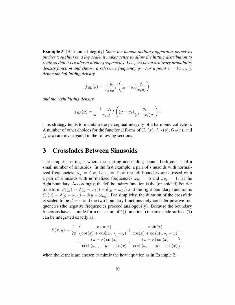
3 Crossfades Between SinusoidsThe simplest setting is where the starting and ending sounds both consist of asmall number of sinusoids. In the first example, a pair of sinusoids with normal-ized frequencies ωL1 = 5 and ωL2 = 12 at the left boundary are crossed witha pair of sinusoids with normalized frequencies ωR1 = 6 and ωR2 = 11 at theright boundary. Accordingly, the left boundary function is the (one-sided) Fouriertransform S0(y) = δ(y − ωL1) + δ(y − ωL2) and the right boundary function isSπ(y) = δ(y − ωR1) + δ(y − ωR2). For simplicity, the duration of the crossfadeis scaled to be d = π and the two boundary functions only consider positive fre-quencies (the negative frequencies proceed analogously). Because the boundaryfunctions have a simple form (as a sum of δ() functions) the crossfade surface (7)can be integrated exactly as

S(x, y) =1

2π

(x sin(x)

cos(x) + cosh(ωR2 − y)+

x sin(x)

cos(x) + cosh(ωR1 − y)...

+(π − x) sin(x)

cosh(ωL2 − y)− cos(x)+

(π − x) sin(x)

cosh(ωL1 − y)− cos(x)

)when the kernels are chosen to mimic the heat equation as in Example 2.

10

This is plotted in Fig. 3(a). The boundaries at the left and right show thetwo sinusoids (as delta functions at their respective frequencies) while the surfacegradually descends to the middle where they meet. Observe that there are twoshapes that connect the nearby frequencies ωL1 to ωR1 and ωL2 to ωR2 . Theseare local maxima (in the y direction) which form a connected set as x varies overits range; call these ridges. Observe that there is a significant loss of height inthe ridges of Fig. 3(a). Since the magnitude of the surface corresponds to theamplitude of the spectral components, this may be perceptible as a drop in thevolume towards the middle of the crossfade region.

Figure 3: Sinusoids of frequencies ωL1 = 5 and ωL2 = 12 are crossed withfrequencies ωR1 = 6 and ωR2 = 11 using the Poisson kernel and three differentG(x) functions (see text for details). Though the ridges connecting the nearbyfrequencies appear in all three figures, the drop in (a) is likely to be heard as adrop in volume over the course of the first half of the crossfade.

11

Figure 3(b) also uses the Poisson kernel (4) but definesGL(x) = (π−x) sin(x)and GR(x) = x sin(x). This tends to increase the total mass in the middle of thecrossfade, and the ridge sags less than in (a). Figure 3(c) defines

GL(x) = GR(x) = sin(x) (8)

which boosts the ridge to a (near) constant height as it spans the duration to con-nect the sinusoidal pairs on the two boundaries. Observe that in all three casesthe sinusoids sweep smoothly from their starting to their ending frequencies. Incontrast, a linear combination of the two sounds (as in the cross fade of Example1) has no ridges: the amplitudes of the two starting frequencies die away to zeroover the duration of the fade while the amplitudes of the two ending frequenciesslowly increase.

The kernels used in Fig. 3 have the same width at all frequencies y, whichmay not be desirable when attempting to cross more complex sounds. Considera source sound with partials at (relative) frequencies 8, 16, 32 and 64 and a desti-nation sound with partials at 9, 18, 36 and 72. If these sounds are to be spectrallycrossed, it is desirable to have 8→ 9, 16→ 18, 32→ 36, and 64→ 72. With anequal width between all pairs, this is impossible since the distance between 9 and16 (two partials which should not be connected by a ridge) is less than 8 while thedistance between 64 and 72 (two partials which should be connected by a ridge)is 8. This is shown in the left side of Fig. 4. While the lower ridges appear asexpected, the upper two pairs are not joined together by a ridge. Once again, thefreedom to modify the kernels allows a solution. The right hand side of Fig. 4shows a kernel, as suggested by Example 3, that is narrow at lower frequenciesand wider at higher frequencies, allowing ridges to form for all the pairs. Thespecific kernel used is

f(x, y) =sin(x)

cosh( y−y00.12y0

)− cos(x), (9)

which scales the f(x, y) values so that they stretch more for larger y.The above discussion emphasizes the importance of the ridges, and it is crucial

to be able to make good choices of kernels that lead to desirable ridges. While it isdifficult to prove in general when ridges will occur and how wide they are, in thesimple case where the kernel is a rectangle function, the existence and behaviorof ridges can be described analytically. Viewing the smooth kernels as havinga support that can be approximated by an appropriate set of rectangle functions

12

Figure 4: The ridges in the crossfade surface on the left are equally wide irrespec-tive of the absolute frequency. In some situations, it may be advantageous to allowthe width of the ridges to become wider at higher frequencies, as shown on theright. This can be accomplished by defining the kernels as suggested in Example3.

suggests that insights gained from studying the rectangle kernels may be useful inmore general situations.

The rectangle function rect(x) is defined as one for x ∈ (−1/2, 1/2) and zerootherwise. For a > 0, let f(x) = arect(ax) and define the kernel as in Example3. The support of the left boundary hitting density is [y − xy

ay0, y + xy

ay0] and the

support of the right boundary hitting density is [y − (d−x)yay0

, y + (d−x)xyay0

]. Thesupport of the left density varies linearly in x (if y is held constant) from zero atx = 0, to a maximum of 2dy/y0a at x = d (and similarly for the support of theright density). Consider the crossfade between a pure frequency ωL on the leftboundary to a pure frequency ωR on the right boundary. Thus S0(y) = δ(y − ωL)and Sd(y) = δ(y − ωR). The crossfade surface is

S(z) =(1−G(x))fz|L(ωL) +G(x)fz|R(ωR)

=(1−G(x))a

x

y0y

rect(a(ωL − y)

y0xy

)+G(x)

a

d− xy0y

rect(a(ωR − y)

y0(d− x)y

)

13

A ridge is said to exist whenever there is a trajectory T = {(x, y(x)) : ∀x ∈[0, 1] such that both terms in the above expression are nonzero}.

Theorem 1 (The Ridge Theorem) Suppose that ωR > ωL and that d < 2ay0. Aridge exists if and only if

ωRωL

< 1 +d

2ay0. (10)

A proof is given in Appendix A.1.

4 Audio CrossfadesThis section presents a series of experiments that carry out generalized crossfadesbetween a variety of sounds, including sinusoids, instrumental, and environmentalsounds. The experiments demonstrate the ridge theorem concretely by showingthe interaction between the width of the kernel and the frequencies joined by theridges. To be practical, it is desirable to have ridges that connect partials of thestarting and ending sounds when the frequencies are close and to not have ridgeswhen the frequencies of the partials are distant.

In order to implement the crossfade procedure, it is necessary to discretize thetwo dimensions, to choose the size n of the FFTs that will be used to specify theboundary spectra, and to select a window that will extract the n samples from thesound waveforms. These choices are familiar from short-time Fourier transform(STFT) modeling [11], and the same tradeoffs apply. In addition, n must be equalto the number of points in the vertical y direction. We have found n = 210, 211,and 212 to be convenient and have used a standard Hann window. In the horizontalx direction we have typically used between m = 200 and m = 500 points.

The inversion of the two-dimensional surface S(x, y) of (7) into a sound wave-form can be accomplished using any of the techniques that would invert an STFTimage into sound. The sound examples of this section implement a “phase vocoder”strategy that is well known in applications such as time scaling and pitch trans-position [2], [8], [14]). This method synthesizes phase values for a given setof magnitude values, effectively choosing phase values that guarantee continuityacross successive frames. To be explicit, suppose that the frequency fi is to bemapped to some value g. Let k be the closest frequency bin in the FFT vector,i.e., the integer k that minimizes

∣∣k srn− g∣∣ where sr is the sampling rate. Then

the kth bin of the output spectrum at time index j + 1 has magnitude equal to the

14

magnitude of the ith bin of the input spectrum with corresponding phase

θj+1k = θjk + 2π dt g (11)

where dt is the time separation between consecutive frames. The phase values in(11) guarantee that the resynthesized partials are continuous across frame bound-aries, reducing the likelihood of discontinuities and clicks. An advantage of thisapproach is that it allows the duration of the fade to be freely chosen after the so-lution to the crossfade surface has been obtained. Thus the relationship betweent∗ in Fig. 2 and real time can be freely adjusted even after the calculation of thesurface S(x, y).

A series of generalized crossfades demonstrate that the ridges of Figures 3 and4 are perceived as pitch glides. Sound examples 220to230.wav, 220to240.wav, through 220to270.wav are available at the website [18] (as are all othersoundfiles discussed throughout the paper). All examples use the kernel f(x, y)in (9) and the transition function G(x) of (8). In each case, the crossfade startsat the pitch corresponding to the first frequency and rises smoothly to the pitchcorresponding to the second frequency, as shown graphically in Fig. 5(a). Thefrequency values are calculated from the output of the phase vocoder using ananalysis that interpolates three frequency bins in each FFT frame. In these graphs,the method is accurate to about 2 Hz (far better than the 44100

2048≈ 22 Hz resolution

of the FFT bins).When the frequencies of the sinusoids at the start and end are far apart, there

is less interaction. The sound example in 220to300.wav begins as a sine waveat 220 Hz and ends as a sine wave at 300 Hz. What happens is that the startingsinusoid decreases in amplitude and the ending sinusoid increases in amplitudethroughout the process. Essentially, the kernel is no longer wide enough to formridges and the connecting sound has become a simple crossfade. The instanta-neous frequencies of the two sines are shown in Fig. 5(b), which shows that bothsines are individually identifiable throughout the process. The pitches are notcompletely fixed at 220 and 300, but bend slightly towards each other. The fi-nal sinusoidal example shows how superposition applies to the crossfade processwhen the sine waves are far apart in frequency. In the example 220to260+440to400.wav, a sine at 220 glides smoothly to 260 while a sine at 440 glidessmoothly to 400. The two are effectively independent. Indeed, the output to thetwo crossfaded pairs is (almost exactly) the sum of outputs to the two pairs cross-faded separately.

15

220

230

240

250

260

270

time(a) (b)

freq

uen

cy H

z

start of

morphs

end of morphs

220

240

260

280

300

time

start of morph end of morph

Figure 5: (a) Six different crossfades begin at 220 Hz and proceed to 220, 230,240, 250, 260, and 270 Hz. Each sounds like a single sine wave that slowlyincreases in pitch up to the specified frequency. (b) A sinusoid at 220 Hz is cross-faded with a sinusoid at 300 Hz. Because the pitches only bend slightly, theprocess is almost indistinguishable from a simple amplitude crossfade.

4.1 Instrumental and Environmental CrossfadesThe crossfades in this section are conducted as interpolation crossfades, whichstretches time proportional to the x-width of the surface S(x, y). Again, the kernelused is f(x, y) of (9) and the transition function G(x) is (8). The first two exam-ples cross between single-tone instrumental sounds. In morph-PianoClarinet.wav, an A2 attack on the piano changes slowly into a sustained A2 on the clar-inet. Similarly, in morph-ViolinTrumpet.wav, both instruments play a C4as the attack of the violin crossfades into the sustained portion of the trumpet.Two spectrally rich sounds, a chinese gong and a low C on a minimoog synth,are crossed in morph-GongMinimoog.wav. Several nonobvious effects canbe heard including the rising and falling pitch contours, and the slow swelling ofthe low C towards the end. Then in morph-GongLion.wav, the same gongrecording is crossed with the roar of a lion. Spectrally rich sounds seem to cross-fade particularly well.

Multiphonics occur in wind instruments when the coupling between the driver(the reed or lips) and the resonant tube evokes more than a single fundmantalpitch. The sounds tend to be inharmonic and spectrally rich, the timbres rangefrom soft and mellow to noisy and harsh. We recorded Paris-based instrumentalistCarol Robinson playing a large number (about 80) of multiphonics. These rangedin duration from brief (a few hundred milliseconds) to fully sustained (several

16

seconds). The timbres ranged from soft and mellow to noisy and harsh. For thepresent application, a number of these were selected, and sustained crossfadeswere calculated between a variety of starting and ending multiphonics. These are

morph-MultiXMultiY.wav

where (X,Y) take on values (13, 23), (29, 66), (32, 14), (39, 28), (48, 64), and(74, 53). All of these can be heard (along with the original recordings of themultiphonics) on the website for the paper [18]. Despite the variety of startingand ending timbres, the crossfades connect smoothly. There are partials that movein frequency (as suggested by the experiments of Sec. 3) and the basic level ofnoisiness in some of the samples also changes smoothly throughout the process.

4.2 Repetitive CrossfadesInterpolation crossfades tend to change the timbre of the sounds in proportion tothe amount time is stretched. Repetitive crossfades more closely parallel visualmorphing since the output is a collection of sounds that are each the same du-ration as the sounds A and B. In this case the sounds are not partitioned intoframes and the boundaries of the crossfade surface are the complete spectra of thesounds. Each column of the solution S(x, y) represents the spectrum of a differentintermediate sound.

This distinction has several implications. First, the sounds cannot be too longsince they must be analyzed (and inverted) all at once; at the normal CD samplingrate, this limits the duration to a few seconds. Second, the horizontal axis needsonly have as many points as the desired number of output (intermediate) sounds(recall that for the interpolation crossfades, there needs to be as many mesh pointsas there are frames in the duration t). Thus, while the frequency y dimension issignificantly larger, the time dimension x is significantly smaller. It is possibleto be clever. Appendix A.2 shows how, when using the Poisson kernel (4), it ispossible to calculate the crossed signal at the midpoint d/2 without calculatingthe complete surface, that is, to calculate S(d/2, y) in isolation. This can reducethe numerical complexity significantly. The method of the Appendix can also beiterated to yield the solutions for S(d/4, y), S(3d/4, y), etc.

Perhaps the greatest difference is in the reinterpretation of the S(x, y) intosound. In the interpolation crossfade, it is necessary to reconstruct the phasesof the spectra in some way (for instance, using the phase vocoder strategy as in(11)). In the repetitive crossfade, it is possible to use the complete complex-valued

17

spectra as the boundary conditions; the surface S(x, y) becomes complex-valuedand each column represents the complete spectrum of the sound.

The first two examples of the repetitive crossfade are between single-tone in-strumental sounds. In repmorph-PianoClarinet.wav, anA2 attack on thepiano is crossed with an A2 on the clarinet. Each of the sounds was truncated toabout 2.5 seconds, and nine different intermediate sounds were generated. In thesoundfile, each of the nine sounds is separated by about 0.25 seconds of silence.The first sound is the trumpet (sound A), the last is the clarinet (sound B), andthe others are the intermediaries. Similarly, in repmorph-TrumpetViolin.wav, both instruments play a C4 as the attack of the trumpet is crossed into theviolin.

Two spectrally rich sounds, a chinese gong and a low C on a minimoog synth,are crossed in repmorph-MinimoogGong.wav. The first 2.5 second sound isthe minimoog note, and the next several slowly incorporate increasing amount ofgong noise. The final segment is the pure gong sound. Observe that this is quitea different set of effects from the interpolation crossfades of the same sounds.In repmorph-Gong1Gong2.wav, two different gong sounds are faded to-gether, creating a variety of “new” intermediate gong-like sounds. Finally, inrepmorph-LionGong.wav, the same gong recording is crossed with the roarof a lion. Spectrally rich sounds cross easily, and the middle sounds are plausiblehybrids.

5 ConclusionBy formalizing the idea of a crossfade function as one which smoothly connectstwo signals, this paper provides a basis for studying processes that underly soundtransitions. The use of a variety of kernels is key, as this specification connectsa family of uninteresting transitions (such as simple crossfades) with more inter-esting transitions (such as spectral crossfades). The ridge theorem delineates ina simple setting when spectral peaks in one signal connect to those in another.The methodology (of regarding the spectrogram as a surface defined by hittingpoints of a stochastic process) provides some hope that similar questions can alsobe handled analytically. The mathematics is applied concretely to the problemsof interpolation and repetitive crossfades, and each is demonstrated in a handfulof sound examples where the strengths and weaknesses of the approach becomeapparent. In many of the examples, it is possible to clearly hear the ridges, in-dicating that these plausibly correspond (in an audio sense) to the smooth ridges

18

that appear in Figures 3-4.

6 AcknowledgementsThe authors would like to thank Howard Sharpe for extensive discussions duringthe early phases of this project.

A Appendix

A.1 Proof of the Ridge TheoremFix a value of x in the interval [0, d]. There is a nonzero contribution from bothterms as long as the upper part of the rectangle for the first term extends furtherthan the lower part of the rectangle for the second term. The y value for where theupper part of the rectangle for the first term terminates satisfies

(y − ωL)ay0xy

=1

2

y =ωL

1− x2ay0

.

Similiarly the y value for where the lower part of the rectangle for the second termterminates satisfies

(y − ωR)ay0

((d− x)y=− 1

2

y =ωR

1− d−x2ay0

.

Thus the condition for overlap is

ωL1− x

2ay0

>ωR

1− d−x2ay0

ωRωL

<2ay0 + (d− x)

2ay0 − x

It is easy to verify that the right hand side of the above inequality is increasing in xand thus takes on its minimum value at x = 0. This gives the theorem statement.∆

19

A.2 A Computational SimplificationLet P (x, y) be the Poisson kernel (4). The line where x = d/2 = π/2 representsthe center strip of the crossfade surface. A Brownian motion started on this centerstrip has the hitting distribution

fπ/2(y) =1

2π(P (π/2, y)1L + P (π − π/2, y)1R)

=1

2π(

1

cosh(y)1L +

1

cosh(y)1R)

=1

2π(

2 exp(|y|)exp(2|y|) + 1

)(1L + 1R).

To find the characteristic function or Fourier Transform of this probability density

zx(y) =P (x, y)

2(π − x)

=1

2(π − x)

sin(x)

cosh(y)− cos(x).

The following transform pair can be found in [10], Table 1A, Even Functions, #201:

f(x)⇐⇒g(y)

1

2N

1

cosh(ax) + cos(b)⇐⇒ 1

N

1

aπ csc(b)

sinh( bya

)

sinh(πya

)

where N = ba

csc(b)b < π. Letting a = 1, b = π − t, and N = (π − t) csc(π − t)gives the transform relation

1

cosh(x)− cos(t)⇐⇒ 2π

sin(π − t)sinh[(π − t)y]

sinh[πy]

Hence,

zx(y) =1

2(π − x)

sin(x)

cosh(y)− cos(x)

⇐⇒ π

(π − x)

sin(x)

sin(π − x)

sinh[(π − x)ω]

sinh[πω]

=π

(π − x)

sinh[(π − x)ω]

sinh[πω]

= Zx(ω)

20

where Zx(ω) is the characteristic function (and Fourier Transform since we aredealing with even functions) of zx(y).

References[1] F. Boccardi and C. Drioli, “Sound Morphing With Gaussian Mixture Models,”

Proc. 4th COST G-6 Workshop on Digital Audio Effects, Limerick, Ireland,Dec. 2001.

[2] M Dolson, “The phase vocoder: a tutorial,” Computer Music Journal, Spring,Vol. 10, No. 4, 14-27, 1986.

[3] T. Erbe, Soundhack Manual, Frog Peak Music, Lebanon, NH, 1994 (pp. 7-40).

[4] E. Farnetani and D. Recasens, ”Coarticulation and Connected Speech Pro-cesses,” in Handbook of Phonetic Sciences, 2cnd Edition, Ed. W. J. Hardcas-tle, J. Laver, F. E. Gibbon, Blackwell Pubs. 2010 (pp. 316-352).

[5] K. Fitz, L. Haken, S. Lefvert, and M. O’Donnell, “Sound morphing usingLoris and the reassigned bandwidth-enhanced additive sound model: Practiceand applications,” in International Computer Music Conference, Gotenborg,Sweden, 2002.

[6] K. E. Gustafson, Introduction to Partial Differential Equations and HilbertSpace Methods, John Wiley and Sons, Hoboken, NJ, 1980 (pp. 1-35).

[7] W. Hatch, High-Level Audio Morphing Strategies, MS Thesis, McGill Uni-versity, Aug. 2004.

[8] J. Laroche and M. Dolson, “Improved phase vocoder time-scale modificationof audio,” IEEE Trans. on Audio and Speech Processing, Vol. 7, No. 3, May1999.

[9] R. J. McAulay and T. F. Quatieri, “Speech analysis/synthesis based on a si-nusoidal representation,” IEEE Trans. on Acoustics, Speech, and Signal Pro-cessing ASSP-34(4), 744-754, 1986.

[10] F. Oberhettinger, Fourier Transforms of Distributions and Their InversesAcademic Press, New York, 1973 (pp. 15-17).

21

[11] A. V. Oppenheim and R. W. Schafer, Discrete-Time Signal Processing, 3rdEdition, Prentice-Hall, New Jersey, 2009 (pp. 730-742).

[12] L. Polansky, and M. McKinney, “Morphological mutation functions: ap-plications to motivic transformations and to a new class of cross-synthesistechniques,” Proc. of the ICMC, Montreal, 1991.

[13] X. Serra, “Sound hybridization based on a deterministic plus stochastic de-composition model,” in Proc. of the 1994 International Computer Music Con-ference, Aarhus, Denmark, 348351, 1994.

[14] W. A. Sethares, Rhythm and Transforms, Springer-Verlag, London, UK 2007(pp. 111-145)

[15] W. A. Sethares, A. Milne, S. Tiedje , A. Prechtl and J. Plamondon, “Spectraltools for dynamic tonality and audio morphing,” Computer Music Journal,Vol. 33, No. 2, Pages 71-84, Summer 2009.

[16] M. Slaney, M. Covell, and B. Lassiter, “Automatic audio morphing,” Proc-ceedings of the 1996 International Conference on Acoustics, Speech, and Sig-nal Processing, Atlanta, GA, May 1996.

[17] E. Tellman, L. Haken, B. Holloway, “Timbre morphing of sounds with un-equal numbers of features” Journal of the Audio Engineering Society, Vol. 43,No. 9, 678-689, Sept. 1995.

[18] Sound examples accompanying this paper may be found at http://sethares.engr.wisc.edu/papers/audioMorph.html (date lastviewed July 10, 2015)

22