Kernel Methods for Small Sample andAsymptotic Tail Inference for Dependent,

Heterogeneous Data

[Running Title: Kernel Methods for Tail Inference]

Jonathan B. Hill¤

Dept. of EconomicsFlorida International University, Miami, FL

March 17, 2007

Abstract

This paper considers tail shape inference techniques robust to sub-stantial degrees of serial dependence and heterogeneity. We detail a newkernel estimator of the asymptotic variance and the exact small samplemean-squared-error, and a simple representation of the bias of the B. Hill(1975) tail index estimator for dependent, heterogeneous data.

Under mild assumptions regarding the tail fractile sequence, mem-ory and heterogeneity, choosing the sample fractile by non-parametricallyminimizing the mean-squared-error leads to a consistent and asymptoti-cally normal estimator.

A broad simulation study demonstrates the merits of the resultingminimum MSE estimator for autoregressive and GARCH data. We ana-lyze the distribution of a standardized Hill-estimator in order to asses theaccuracy of the kernel estimator of the asymptotic variance, and the distri-bution of the minimum MSE estimator. Finally, we apply the estimatorsto a small study of the tail shape of equity markets returns.

1. INTRODUCTION The use of extreme value theory has reachedinto risk management in …nance, damage and catastrophe modeling in the en-gineering, actuarial and meteorological sciences, and the analysis of asset mar-ket contagion and hyper-in‡ation. See, e.g., Mandelbrot (1963), Fama (1965),McCulloch (1996), Embrechts, Klüppelberg, and Mikosch (1997), Finkenstadt

¤Dept. of Econom ics, Florida Internat ional University, Miami, FL; www.…u.edu/»hill jona ;jonathan.hil l@…u.edu.AMS classi…cation: 62G32.Keywords : Hill est imator; regular variation; extremal near epoch dependence; kernel est ima-tor; mean-square-error.

1

and Rootzén (2003), Bradley and Taqqu (2003), Rachev (2003), and Beirlant,Goegebeur, Segers, Teugels, and De Waal (2004).

The general framework for analyzing extremes begins by assuming the dis-tribution tail is regularly varying at 1: there exists some 0 such that forall

¹() := () =¡()0where is slowly varying. (1)

Distributions satisfying (1) include the domain of attraction of the stable lawswith 2, coincide with the maximum domain of attraction of the extremevalue distributions expf¡¡g, and characterize the tails of GARCH processes.See deHaan (1970), Leadbetter, Lindgren and Rootzén (1983), Bingham, Goldieand Teugels (1987), Resnick (1987), and Basrak, Davis, and Mikosch (2002).

Denote by () 0 the order statistic of the sample path f1g:(1) ¸(2) ¸ , and let= fg2N denote a sequence of integers satisfying ! 1 as ! 1, and = (). B. Hill (1975) proposed the followingestimator of ¡1:

¡1

:= 1X

=1ln()(+1)

The Hill-estimator has been widely used in the economics, …nance, and telecom-munications literatures, in particular on data for which substantial evidencesuggests serial dependence and/or heterogeneity via volatility clustering. SeeAkgiray and Boothe (1988), Cheng and Rachev (1995), Resnick and Rootzén(2000) and Chan, Deng, Peng and Xia (2005) and Hill (2005b), to name a veryfew.

The question of selecting the tail fractile for dependent, heterogeneousdata, however, remains entirely ignored. Tail fractile selection is a long stand-ing problem in the extreme value theory literature because tail shape and taildependence estimates may be highly sensitive to the chosen tail region. See Fig-ure 1 for plots of ¡1

and ¡1[] for iid, AR(1) and IGARCH data with Stable

or Pareto innovations. Positive serial dependence increases the likelihood thatneighboring observations are close in value, diminishing observable tail thick-ness and rendering the Hill-estimator positively biased (e.g. Stable AR(1));volatility clustering augments the detectable degree of tail thickness, leading tonegatively biased estimates (e.g. Pareto IGARCH). Such plots are essentiallynon-formative for dependent or heterogeneous data.

INSERT FIGURE 1 HERE

Graphical "Hill-plot" methods for tail fractile selection for iid data are con-sidered at length in Renick and St¼aric¼a (1997) and Drees, de Haan, and Resnick(2000). See, also, Beirlant, Vynckier and Teugels (1996) and Beirlant, Dierckx,and Guillou (2005). Bootstrap and adaptive selection methods for selecting in the iid case are considered in Hall and Welsh (1985), Hall (1990), Drees andKaufman (1997), and Draisma, de Haan, Peng and Periera (1997).

2

Mean-squared-error (MSE) and bias reduction methods for selecting are developed in the seminal contributions of Hall (1982) and Hall and Welsh(1985), and recently in Beirlant,Vynckier and Teugels (1996), Resnick andSt¼aric¼a (1997), Danielsson, de Haan, Peng, and de Vries (1998), Hall (1990), andHuisman Koedijk, Kool, and Palm (2001). An iid assumption is universally im-posed in this literature, and several methods are suggested without theoreticalriguer. Consider Beirlant,Vynckier and Teugels (1996) and Huisman, Koedijk,Kool, and Palm (2001).

It is a possible misconception that selecting the sequence fg by minimiz-ing the MSE for each leads to a inconsistent estimator . Hall (1982) andHall and Welsh (1985) use the tail shape

() =¡(1 +(¡))0 (2)

and focus on sequences » 2(2+) , 0. The MSE is easy to char-acterize for iid data, and is parametrically minimized with respect to . Theresulting estimator is inconsistent due simply to the chosen class of fractiles2(2+). See Hall (1982: Theorem 2) and Hsing (1991: Theorems 2.4). Seealso Huisman et al (2001).

In this paper we analyze non-parametric methods for selecting the tail frac-tile for the B. Hill (1975) estimator for processes with substantial degreesof dependence and heterogeneity restricted only to extremes. We do not im-pose any structure on non-extremes. For processes satisfying (1) we discussa consistent kernel estimator of the exact MSE and asymptotic variance. Wethen characterize the small sample bias for tails satisfying (2), construct a bias-corrected MSE, and select fg by minimizing the MSE.

We only consider a class of sequences fg for which the Hill-estimator isknown to be consistent and asymptotically normal under general conditions, cf.Hill (2005a). The class (2) is not too restricted, and includes stochastic recur-rence equations, including the marginal distributions of Multivariate GARCHprocesses. See Basrak et al (2002).

We focus on the Hill-estimator because a broad asymptotic theory alreadyexists for dependent, heterogeneous data. The minimum MSE estimator is con-sistent and asymptotically normal for processes fg with extremes that areNear-Epoch-Dependent on themixing extremes of some shock process fg. Thiscovers at least nonlinear distributed lags, ARFIMA() and FIGARCH()processes with fractional di¤erence 2 [01), bilinear processes, and randomcoe¢cient and threshold autoregressions. Apparently this is the most generaltheory available for this or any other tail estimator (e.g. Pickands 1975; Smith1987; Drees, Ferreira, and de Haan 2004), and for this or any other fractile se-lection method (e.g. Hall and Welsh 1985; Drees, de Haan, and Resnick 2000).

In a large scale simulation study we analyze the merits of the kernel MSEestimator, say 2

, for sample fractile selection. We also analyze 2

as an

estimator of the asymptotic variance. We perform Cramer-von Mises tests ofstandard normality on standardized ratios ´ p(¡1

¡ ¡1) and

…nd the range of over which ¼ (01) at the 5%-10% levels nearly alwaysincludes the optimally selected by minimizing the MSE.

3

Section 2 lays out extremal dependence de…nitions and properties of theHill-estimator. In Sections 3 and 4 we characterize the mean-squared-error andbias of the Hill estimator for general data. Section 5 presents fractile selectionmethods and key asymptotic theory. Sections 6 and 7 contain a simulationstudy and an application to daily equity market returns. All …gures and tablesare placed at the end of the paper.

2. TAIL SHAPE AND TAIL MEMORY We assume has for eacha common marginal distribution tail (1) with support on [01), and -…eld== ( : · ). In practice this setting applies to an absolute series =jj, or tail preserving transforms = ¡£ (0) and = £ (0).

Assume ¹()¹(¡) ! 1 such that there exists sequences fg 1 andfg 1, ! 1, satisfying

()() ! 1 (3)

See Leadbetter et al (1983: Theorem 1.7.13). We must restrict the tail shape inorder to expedite asymptotic normality. Cf. Goldie and Smith (1987: propertySR1), Hsing (1991) and Hill (2005a).

Assumption A fg satis…es (1) for some 0. For some positive measur-able : R+ ! R+,

()() ¡ 1 = (()) as ! 1 (4)

The function has bounded increase: there exists 0 0 1 and 0 such that ()() · some for ¸ 1 and 0Speci…cally,fg 1 , fg 1, and (¢) satisfy

p() ! 0where ! 1, = (). (5)

Remark 1: Tails satisfying Assumption A include ¹() = ¡(1 +((ln)¡)) and ¹() =¡(1 + (¡)). See Haeusler and Teugels (1985).Tails of the latter form have been widely exploited in the applied and theoreticalstatistics and econometrics literatures, and characterizes the tails of GARCHprocesses. See Hall (1982), Hall and Welsh (1985), Chan and Tran (1989), Caner(1998), Basrak et al (12002) and Hill (2005b) to name a new.

Remark 2: Property (5) restricts the rate at which ! 1, and is keyto ensuring consistency and asymptotic normality for for general classes ofdata. See Hsing (1991) and Hill (2005a). If, for example, the tail satis…es (2)then (5) holds if

=(2(2+))

See Haeusler and Teugels (1985) for this and other examples. Property (5),therefore, does not include the sequence » 2(2+) exploited in Hall

4

(1982), Hall and Welsh (1985) and Huisman et al (2001). Such sequences render an inconsistent estimator of . See Hall (1982) and Hsing (1991).

We require extremal versions of mixing and Near-Epoch-Dependence proper-ties developed in Hill (2005a). Consult that source for complete details, and seeHall and Heyde (1980) and Gallant and White (1988) for details on conventionalmixing and NED processes.

Denote by = fg a sequence of constant real thresholds, ! 1 as! 1, and denote by ´ () a measurable extremal functional of for 2 f1g, and = 0 for any other 2 f1g. Examples includethe extreme event (jj ), exceedance (jj ¡)+, and value jj £(). De…ne

z:=(() : ··)

and de…ne the coe¢cients

´ sup2z+2z+1

+:2Zj(\ +) ¡()(+)j

´ sup2z+2z+1

+:2Zj(+j) ¡(+)j

where fg is a sequence of positive integers satisfying 1 · · , ! 1 as! 1 and = ().

E-Mixing If ! 0 as ! 1 we say fg is Extremal-Strong Mixing withsize 0. If ! 0 as ! 1 we say fg is Extremal-uniformmixing with size 0.

2-E-NED fg is -Extremal-NED on some array of -…elds fz1g with

size 0 , 0, if for any 2 R°°(

j=+¡) ¡(

jz+¡)

°°

·()

where : R ! R+ is Lebesgue measurable on R+, sup() = (()1)for each 2 R, and ()1¡1 ! 0 for some .

Remark 1: fg is E-NED on fg if extremal information induced byextremes of can be used to forecast the extreme event with analmost surely zero prediction error as ! 1. Memory restrictions are notimposed on the non-extremal support: · ! 1.

Remark 2: The E-NED property allows for a large degree of extremaland non-extremal memory and heterogeneity, including ARFIMA() andFIGARCH() processes with 2 [01)bilinear processes, nonlinear dis-tributed lags, random coe¢cient autoregressions, and extremal threshold au-toregressions. See Hill (2005a: Section 5). Thus, random walk and IGARCHprocesses have not been shown to have near epoch dependent extremes.

5

Assumption B fg is 2-E-NED with size 12 on an E-Mixing process fg.The base fg is E-Uniform Mixing with size [2(¡ 1)] for some ¸2, or E-Strong Mixing with size (¡ 2) for some 2.

Under Assumptions A and B, Theorem 5 of Hill (2005a) deliversp

¡¡1

¡¡1¢ ) (01) and

p( ¡)~ )(01)

where2

:= (p(¡1

¡¡1))2 and ~2

=42

3. MEAN-SQUARED-ERROR KERNEL ESTIMATOR Note 2

is identically the asymptotic variance and exact small sample MSE of ¡1

. Ifthe data are iid then Hall (1982) shows2

!¡2. In general when an analytic

expression for 2

is not available Hill (2005a) proposes a kernel estimator

2 =¡1

X

=1

X

=1((¡))

where := [¡ln(+1)

¢+ ¡ ()¡1

], and ((¡ )) denotes a

standard kernel function with bandwidth 1 · ! 1 as !1.

Assumption C Let 12 ! 1, ! 1 as ! 1, = (¡12),and 1

P=1 j((¡ ))j = (12). Moreover, (¢) satis…es

Assumption 1 of de Jong and Davidson (2000).

Under Assumptions A-C, Theorem 6 of Hill (2005a) delivers

j2 ¡2

j ! 0

This includes Bartlett, Parzen, Quadratic Spectral and Tukey-Hanning kernels.The estimator 2

alone, provides an enormous improvement in theory

over existing MSE representations in which an iid assumption is universallyimposed, leading to a potentially massive underestimate of the true MSE of¡1 for highly dependent and heterogeneous data. See Section 6 for evidence.

Nevertheless, notice that 2 incorporates the possibly biased ¡1

in fg.In the next section we exploit a new characterization of the small sample biasto improve both ¡1

and the MSE for small samples.

4. SMALL SAMPLE BIAS The small sample bias is exactly

:= (p(¡1

¡¡1))

If » (2) such that () = ¡(1 + ¡+ (¡)), and »

2(2+)then Hall (1982: Theorem 2) proves ! ¡+12(+ ). Under Assumptions A and B, however, the Hill-estimator is asymptoti-cally unbiased.

6

THEOREM 1 Under Assumptions A and B

=p£¡1 [(1 +(()))

2 ¡ 1] +(1) =(1) (6)

Inspecting (6), a simple estimate of the bias can be achieved if the non-parametric term (()) can be expressed analytically. For example, if thetail probability satis…es (2) then Haeusler and Teugels (1985) show

() = ¡

andp() ! 0 if = (2(2+)) = 0. The -quantile

can be easily estimated by thep-consistent (+1), where consistency is

established for processes E-NED on an E-Mixing base in Hill (2005a: Theorem5).

Hall and Welsh (1985) argue that tails (2) typically arise () as powers ofsmooth distributions; () from Type II extreme value distributions expf¡¡g;or () from stable distributions. They argue that case () typically involves = or = 2; case () renders = ; and case () implies = if 1and 2 · if 1 2.

In most cases, therefore, = = 2, or lies in a known range and inmost cases, they argue, ¸ . Hall (1990) and Huisman et al (2001) thereforesimply assume = .

COROLLARY 2 Suppose

¹() =¡(1 +¡)0 (7)

and = (23)Under Assumptions A and B

=p¡1 £5 £¡

+(1)

Remark 1: Under Assumption B tail shape (2) require =(2(2+))= (23) when = .

Remark 2: For small samples and any process satisfying (2), or moregenerally (1), is at best a rough approximation of the true bias. Paretorandom variables, for example, have (¡) = 0, hence over-estimates thebias.

The bias estimator and bias-correct Hill-estimator ¡1() simultane-

ously solve

=p¡1

() £5 £¡()

(+1) (8)

=p¡1

£5 £¡1(¡1

¡p)

(+1)

¡ £5 £¡1(¡1¡

p)

(+1)

¡1

() = ¡1

¡ p

7

The solution f¡1

()g can be computed numerically for each . How-ever, for large samples the mean-value-theorem implies the following result.

LEMMA 3 Under the conditions of Corollary 2 and » , 0 23,if = (

p) then ! 0 and

¯¯¯ ¡

p¡1 £¡

(+1)

2 + £¡(+1) £

¡ln(+1)

¢+¡

(+1)

¯¯¯ ! 0 (9)

The argument used to prove Lemma 3 shows if p degenerates to

zero, then it must be the case that ! 0. In the sequel, therefore, we simplyassert the following.

ASSUMPTION D Any solution f¡1()g to (8) satis…es = (

p)

and ¡1() = ¡1

+ (1) under Assumptions A-B.

Finally, a small sample bias-corrected MSE estimator 2() uses ¡1

():

2

() :=¡1

X

=1

X

=1((¡ )) £ () £ ()

() :=¡ln (+1)

¢+ ¡ ()¡1

()

5. Fractile Selection The simplest criteria for selecting the sample frac-tile is the minimization of the MSE over some set of appropriate sequencesfg. The trick for ensuring both asymptotic normality and consistency is torestrict attention to the set of proportional sequences under Assumption A:

= f= fg2N : ! 1 as ! 1, (4)-(5) hold,= 1 +(1), 8g

The next result shows that f2g is asymptotically equivalent to f~

2~g

for any pair ~2 .

THEOREM 4 Let ~ 2 Under Assumptions A and B, = ~

+ (1p

~)If additionally Assumption C holds, then 2

= 2~

+(1).

Now select that fractile ¤ that minimizes the mean-squared-error 2

orthe bias-corrected the mean-squared-error 2

() for each over some set of

feasible integers µ f1g. Each integer in must belong to asequence fg in .

Under (2) consider

= f= fg, »0 2(2+g

8

For each a candidate set of tail fractile integers is

= fg=1

= f[] ¡1[¡]+g=1, where = 2[¡] + 1

and each 2 N does not depend on above a …xed threshold, set to ensure 1· · for the minimal encountered.

For example, if = 5000 and a rolling-window tail analysis involves windowsof minimum width = 1000, the subset

= f[66 ] ¡ 1 £ [65] +g=1, = 5 £ [65 ] + 1

is valid, where 1000 = f6547g and 5000 = f221544g.The optimal fractile ¤

can be written as

¤= [] ¡ [1¡] +¤, ¤2 f1 g¤= ()

The resulting sequence f¤g 1 is itself an element of . By construction

each

¤= [] ¡ [1¡] +¤2 f [] ¡ [1¡][] + (2 ¡1)[¡]g

hence for any 2

1 á [] ¡ [1¡] +¤[] + (2 ¡1)[¡]

· ¤

· [] ¡ [1¡] +¤

[] ¡ [1¡]! 1

THEOREM 5 Under Assumptions A-C for any subset µ and

¤ 2

©arg min2

2

argmin2 2

()ª

we have p¤(¡1

¤

¡¡1)¤

)(01) and p¤(

¡1¤() ¡¡1)¤

()

) (01).

Remark : Theorem 5 has far more applications than a minimum MSE.Any criterion that selects the fractile sequence from a set of proportional se-quences that satis…es Assumption B will not a¤ect consistency and asymptoticnormality of ¤

, nor consistency of 2

¤.

6. MONTE CARLO STUDY We draw random samples of iid mean-zero innovations fg from either a symmetric Stable distribution with unitscales, or a symmetric Paretian tail

(¡) = () =¡¡1 + 2¡¡1, 2=1492704, 2 [02]

By constructionR 1

¡1()= 1In both cases = 17. Simulation results forother values of are qualitatively similar. We choose = 17 because it is near

9

2 and we want to access the accuracy of tests of …nite variance. The sample sizeis = 1000.

6.1 Step Up

We simulate AR(1) and Power-GARCH(1,1) processes using fg. In theAR(1) case

=¡1 +2 f0269gIn the Power-GARCH(1,1) case

= ¡1, = 0 +1 j¡1j+2¡1= 15

We randomly select 2 [015] from a uniform distribution, retaining onlythose 1 + 2 99.

We simulate 3observations and retain the last . We generate 10000 seriesof each process and compute for the absolute series jj. All reported valuesare averages over all simulated series.

6.2 Estimation

We estimate with accompanying asymptotic 95% con…dence bands us-ing the kernel estimators b~2

= 4

2 with a Bartlett kernel and bandwidth

= [15]. Parzen and Tukey-Hanning kernels produce qualitatively similarresults. We compute the bias according to formula (9), and estimate tailparameters for all 2

= f10550g

See Figure 1, and see Tables 1 and 2 for con…dence band for selected 2 .All reported values are averages over all repetitions.

6.3 Tail Index Estimates

We now return to the issues raised in the introduction. As the degree ofpositive serial dependence increases observations cluster withgreater probabilityhence the observable tail thickness is large. More observations from the tail arerequired to obtain a sharp estimate of for persistent data. Consider Tables1.1 and 2.1. For Stable or Paretian AR(1) processes with = 9 we require atleast = 420 tail observations in order not to incur a Type II error for one-sided tests of ¸ 2 at the 5%-level, and as many as= 510 tail observationswill render a 95% con…dence band that contains = 17. Using = 420 (notshown) the con…dence band for Stable random variables is 168 §24, and using= 510 (not shown) the band is 151 § 19.

In general, for GARCH(1,1) data we require fewer tail observations to obtaina sharp index estimate that autoregressive data with positive serial dependence.This is fairly intuitive: positive serial dependence increases the likelihood ofclustering such that more observations are required to discern the true tailshape (the Hill-estimator is positively biased for small ). On the other hand,volatility clustering augments tail thickness. The use of fewer tail observations

10

in this case improves the likelihood that they will not be neighbors and hencenot strongly heteroscedastically related (the Hill-estimator is negatively biasedfor large ).

6.4 Kernel Asymptotic Variance Estimation

The asymptotic variance of is 2 for benchmark iid random variables.In this case the kernel variance estimator satis…es b~ ¼ for large¸ 350for Stable processes, and even larger ¸ 400 for Paretian tailed processes. Seecolumn one of Tables 1 and 2. As the degree of dependence and heterogeneityincreases, however, the kernel variance increases well beyond 2 . For StableAR(1) processes with iid errors, = 9, and = 400, the kernel estimate isb~ = 408 17.

For exact Pareto tails, ( ) = ¡the performance of the Hill-estimator signi…cantly improves, in particular for iid data. This is well knownin the literature. In simulations not shown here the estimated kernel varianceis between 16 and 18 for any ¸ 50.

Of course this may simply point out the inability of 2 to approximate the

variance of 2

for dependent data. We perform a unique simulation study toassess the merits of 2

by testing how well the standard normal distributionapproximates the true distribution of

=p

¡¡1

¡¡1¢

In this case ¡1

represents the tail index estimate of the series, sayfg1000

=1 , and each series is generated independently of any other series. Weperform Cramer-von Mises tests of standard normality on sequence fg1000

=1for each simulated process.

In Figure 2 we plot Cramer-von Mises test statistics over 2 foriid, AR(1) with = 9 and GARCH(1,1). In general a large number of tailobservations is required to ensure approximate standard normality at the 1%and 5% levels for dependent data, in particular for Stable random variables. Abroad spectrum of fractile values can generate ¼ (01) at the 10%-levelfor GARCH(1,1) data.

6.5 Minimum MSE Estimates

We select the optimal fractile ¤by minimizing the MSE 2

and the bias-corrected MSE 2

(). In general each criterion generates sharp estimates, inparticular for serially dependent data. The optimally selected fractile is nearlyalways within the fractile range over which the Hill-estimator is approximatelynormally distributed at the 5-10% level. See the last two rows of Tables 1 and2.

The only challenging cases involve the minimum bias-corrected MSE esti-mator. The estimator tends to be positively biased for iid and low memory ARdata. Nevertheless, the resulting estimator is exceptional for strongly dependentdata (AR(1) with = 9).

11

7. EMPIRICAL APPLICATION Wenow study daily log-returns fgto the NASDAQ and S&P500 composite indices over the period Jan. 1, 2001to Dec. 31, 2005. Market closures are treated as missing values, and each seriesis …ltered through a standard 5 day dummy regression to remove daily e¤ects.After di¤erencing and removing missing values the sample size is 1422.

See Figure 2 for plots of , and based on the absolute series ´ jjThe only distribution characteristics that matter regarding asymptotics for

(assuming the tails are regularly varying) is dependence and heterogeneity inthe extremes. In order to assess the degree of dependence in the extremes weestimate the …rst order tail dependence coe¢cient (1) de…ned as

(1) := ()((¡1 ) ¡()(¡1 ))

A nonparametric estimator is simply

(1) =1

X

=1

¡((+1)) ¡ ()

¢ ¡((+1)) ¡ ()

¢.

See Hill (2006) for a literature review, asymptotic theory and a robust kernelvariance estimator associated with (1) under Assumptions A-C. Speci…cally,under Assumptions A-C

p((1) ¡(1)) )(01)

where 2

:= (p((1) ¡ (1))2 , and a kernel estimator, a la 2

,satis…es 2

¡ 2

! 0.

Both equity returns series display signi…cant levels of positive …rst orderextremal dependence. Unless we impose a parametric model and explicitly workout a parametric expression for the asymptotic variance of the Hill-estimator (ifone exists analytically), the evidence supports the use of the kernel estimators.

Minimum MSE [MMSE] estimates for either series are close to 2. Non-biascorrected MMSE estimates § 196b~

p are 171 § 204 and 202 §257 for the NASDAQ and SP500, respectively. The "bias-corrected" MMSEestimates are identical to the uncorrected MMSE estimates (up to four decimalplaces) because the estimated bias for each equity market is tiny (between ¡01and ¡12) relative to the magnitude of the MSE itself (between 5 and 80). SeeFigure 3 for plots of ¡1

¡1() and .

Appendix 1: Proofs of Main Results

Proof of Theorem 1. De…ne for any 2 R

fg :=©(ln)+ ¡[(ln )+]

ª(10)

©¤(

p)

ª:=

n³

p

´¡

h

³

p

´io

12

From Lemma A.1 in Appendix 2, Assumptions A and D imply

p

¡¡1 ¡¡1¢ = ¡12

X

=1

¡¡¡1¤

(p)

¢

+p

³1

X

=1(ln)+ ¡¡1

´+

where [¡12

P=1(¡ ¡1¤

(p))] = 0 by construction, =

(1) and [] = (1). Analogous to arguments in Hsing (1991), by properties(1) and (3), dominated convergence and arguments in Smith (1982: eq. 2.2)

£p

¡¡1 ¡¡1¢¤

= p

³1

X

=1(ln)+ ¡¡1

´+[]

=p

µ

(ln)+ ¡¡1¶

+(1)

=p

µ

Z 1

0(

)¡¡1¶

+(1)

=p

µ

()Z 1

1¡1()

()¡¡1

¶+(1)

=p

µ(1 +(())) £

Z 1

1¡1¡(1 +(())) ¡¡1

¶+(1)

=p¡1

³(1 +(()))2 ¡ 1

´+(1)

Proof of Corollary 2. Similar to the above argument, suppose ¹() =¡(1 + ¡£) for some 0Then

£p

¡¡1 ¡¡1¢¤

=p

µ

Z 1

1¡1()¡¡1

¶+(1)

=p

µ

Z 1

1¡1¡

¡(1 +¡¡)¡¡1

¶+(1)

=p

µ

¡

·Z 1

1¡1¡+¡

Z 1

1¡1¡(1+)

¸¡¡1

¶+(1)

=p

µ

¡

£¡1 + (11 +))¡1¡

¤¡¡1

¶+(1)

=p¡1 ¡

(1 +(1p)) £

£1 + (1 +)¡1¡

¤¡ 1

¢+(1)

=p¡1(1 +)¡1¡

+(1)

where = ()(1 + (1p)) by Lemma A.2. Simply put = 1 to

complete the proof.

13

Proof of Lemma 3.

Step 1 ( = (p)): Suppose = (

p). In order to prove

= (1) from (8) we need only show

p

¡1(¡1¡

p)

(+1) =(1)

De…ne := ()

(+1)

and write

(11)

lnµ

()¡1(¡1¡

p)

(+1)

¶

= ¡ ln

1 ¡ £ p

¡ ln()p

£"

£

1 ¡ £ p

#

Under Assumptions A and B, Theorem 1 of Hill (2005b) states

!

and » with 23 implies

(ln)p=

³¡12

ln´

= (1)

Thus, p! 0, ! and (11) imply

()¡1(¡1¡

p)

(+1) ! ¡1

Use 23 ! 0 to conclude

p

¡1(¡1¡

p)

(+1) = (p()) =(1)

Step 2: By the mean-value-theorem there exists for each a randomvariable ¤

2 [0] that satis…es

=p¡1

£5 £¡(+1)

¡5 £ p¡1

£

¡ln(+1)

¢£

¡1(¡1¡¤

p)

(+1)p(¡1

¡¤

p)2£

¡5 £¡1(¡1¡¤

p)

(+1) £

+5 £¤

¡ln (+1)

¢

¡1(¡1 ¡¤

p)

(+1)p(¡1

¡¤

p)2

£

14

Let = (p) such that ¤

! 0 by Step 1: ¤

2 [0 ] ! 0.

Notice (ln(+1)) £ ¡1¡1

(+1) ! 0. Therefore¯¯¯ ¡

p¡1

£¡(+1)

2 + £¡(+1) £

¡ln (+1)

¢+¡

(+1)

¯¯¯ ! 0

Proof of Theorem 4.

Claim 1: Consider©

¤(

p)ª

de…ned in (10). Lemma A.1implies for any (,~) 2

¡12

X

=1

¡¡¡1¤

(p)

¢

¡ (~)12 £ ~¡12

X

=1

³~¡¡1¤

~(p

~)´

= (1)

where (~)12 = 1 + (1) by assumption, hence

¡12

X

=1

¡¡¡1¤

(p)

¢

¡ ~¡12

X

=1

³~¡¡1¤

~(p

~)´

= (1)

Lemma A.3 impliesp

¡¡1 ¡¡1¢ ¡ p

¡¡1 ¡¡1¢

= ¡12

X

=1

¡¡¡1¤

(p)

¢

¡ ~¡12

X

=1

³~¡¡1¤

~(p

~)´

= (1)

Thereforep

¡¡1 ¡¡1¢

¡p

~¡¡1

~ ¡¡1¢

=p

¡¡1 ¡¡1¢³

1 ¡p

~p

´+

p~

¡¡1 ¡ ¡1

~

¢=(1)

By Theorem 5 of Hill (2005a) ¡1 ¡ ¡1 = (1

p), and by assumption

1 ¡p

~p = (1p). We deduce p(¡1

¡ ¡1) = (1), hence

¡1

= ¡1~

= (1p

~) as claimed.

Claim 2: Clearly¯2 ¡ 2

~

¯·

¯2 ¡2

¯+

¯2

~ ¡2~

¯+

¯2 ¡2

~

¯

By Theorem 6 of Hill (2005a) 2 ¡ 2

= (1) for all 2 . Hence, itsu¢ces to prove 2

= 2~

+ (1). This follows from Claim 1: ¡1 = ¡1

~

+ (1p

~) and ~= 1 + (1) 8f, ~g 2 implyp

~¡¡1

~¡¡1¢ ¡ p

¡¡1

¡¡1¢ ) 0

15

in distribution, hence (e.g. Theorem 2.1 of Billingsley, 1999)

2 ¡2

~ =(p(¡1

¡¡1))2 ¡(p

~(¡1~ ¡¡1))2 ! 0

Proof of Theorem 5. The claim follows from Theorem 4, asymptotic nor-mality p(¡1

¡ ¡1) ) (01) and consistency 2

¡2

! 0, cf.

Theorems 5 and 6 of Hill (2005a).

Appendix 2: Supporting Lemmeta

LEMMA A.1 Under Assumptions A and B,

p

¡¡1 ¡¡1¢ = ¡12

X

=1

¡¡¡1¤

(p)

¢

+p

h

³¡1

X

=1(ln)+

´¡¡1

i+

= ¡12

X

=1

¡¡¡1¤

(p)

¢+(1)

where = (1) and [] = (1), and is independent of scale.

LEMMA A.2 Under the conditions of Corollary 2, = ()(1 +(1p)).

LEMMA A.3 Under Assumptions A and B, 8fg 2

1p

X

=1¡ 1

p~

X

=1~=(1)

1p

X

=1¤(

p) ¡ 1

p~

X

=1¤

~(p

~) =(1)

Proof of Lemma A.1. We can always writep

¡¡1 ¡¡1¢

=p

³1

X

=1ln()(+1) ¡¡1

´

=p

³1

X

=1ln() ¡¡1

´¡ p

ln(+1)

=p

³1

X

=1ln() ¡

³1

X

=1(ln)+

´´

¡ p

¡ln(+1)

¢+

p

h

³1

X

=1(ln)+

´¡¡1

i

Using AssumptionA and arguments in Hsing (1991: p. 1554), p[(¡1

P=1 (ln )+)¡

¡1] = (1).Moreover, Lemma 4 of Hill (2005a) and a Cramér-Wold device give

p

³1

X

=1¡11

X

=1¤(

p)

´) (12)

16

where each » (02), 2

1.Furthermore, Lemma 1 of Hill (2005a) states j ln([]) ¡ ln() j ! 0 for

all in an arbitrary neighborhood of 1. Therefore Theorem 2.2 of Hsing (1991:eq. 2.4-2.7) can be used to show

p

³1

X

=1ln() ¡

³1

X

=1(ln )+

´´) 1

p

¡ln (+1)

¢)2

hencep

¡¡1 ¡¡1¢ = 1

p

X

=1

¡¡¡1¤

(p)

¢

+p

h

³1

X

=1(ln)+

´¡¡1

i+

= 1p

X

=1

¡¡¡1¤

(p)

¢+(1)

where

=³1p

X

=1ln() ¡

³1

X

=1(ln)+

´´¡ 1

X

=1

+p

¡ln(+1)

¢¡¡11

p

X

=1¤(

p)

=(1)

Finally [] ! 0 in probability by Fatou’s Lemma: limsup 1[jj] ·[limsup 1 jj] = 0, hence j[]j · [jj] ! 0.

Proof of Lemma A.2. By the construction of the sequence fg 1 andthe distribution tail ¹() = ¡(1 + ¡

) we can write

() » (1 +¡) ) »()

Use = (23) to conclude ()» (1 + ¡1()) = + ()

= + (¡12 ).

Proof of Lemma A.3. For simplicity let ~· 8. Write

112

X

=1¡ 1~12

X

=1 (12)

= 112

X

=1

³¡ (~)12~

´

where

¡ (~)12~

= (ln)+ ¡ (~)12 (ln~)++ (~)12(ln~)+ ¡(ln)+

17

Using Assumption A and (ln )+ ¸ 0, the expectations di¤erence is(12

) because

(~)12(ln~)+ ¡(ln)+ (13)

= (~)12Z 1

0¹(~

)¡Z 1

0¹(

)

= (~)12 ¹(~)Z 1

0

¹(~)¹(~)

¡ ¹()Z 1

0

¹()¹()

» (~)12 ¹(~)Z 1

0¡¡ ¹()

Z 1

0¡

= ¡1 £ ¹()

"µ

~

¶12 ¹(~)¹()

¡ 1

#

= ¡1 £() £(112 ) =(12

)

where the last line follows from ¹() = () by the construction of ,and Lemma A.3.1 below.

It is easy to show · ~ as ! 1 follows from ~· . Assume is su¢ciently large such that · ~. De…ne

1 = f: ~ ¸g, ~2 = f: ¸~g.

Then (12) and (13) imply(14)

¯¯¡12

X

=1

³¡ (~)12~

´¯¯

·¯¯¡12

X

=1

³(ln)+ ¡ (~)12 (ln~)+

´¯¯+(1)

· ¡12

X21

ln

+¯¯¡12

X2~2

³ln ¡ (~)12 ln~

´¯¯ +(1)

· ¡12

X21

ln + (ln~) £ 1~12

X

=1(¸~) +(1)

If we show each term on the right-hand-side of (14) is (1) then the claimis proven by Chebyshev’s inequality. First, as ! 1

°°°°112

X21

ln

°°°°1

·

12

() £Z ln~

0

()()

18

=

12

³1 +(¡12

)´

£Z ln~

0¡

=12

³1 +(¡12

)´

£¡1 £¡1 ¡~

¢

=12

³1 +(¡12

)´

£¡1 £(¡12 ) =(1)

The …rst equality follows from dominated convergence and Assumption A:

( ) » ¡()= () £ (1 +(()))= () £ (1 +(1

p))

The third equality follows from Lemma A.3.1.For the second term in (14), arguments similar to the above and Lemma

A.3.1 give

(ln~) £°°°~¡12

X

=1( ~)

°°°1

· (~¡12 ) £ (~12

) £( )

= (~¡12 ) £ (~12

) £³1 +(¡12

)´

= (1)

LEMMA A.3.1 Under the conditions of Lemma A.3, 82

µ

~

¶12 ¹(~)¹()

= 1 + (¡12 ) and ~

= 1 + (¡12

)

Proof. Properties (1)-(5) imply

() ¹() = ()¡()

= 1 +(()) = 1 +(¡12 )

henceµ

~

¶ ¹(~)¹()

=(~)¡~

()¡

(~)()

=1 +( ~¡12

)

1 +(¡12 )

= 1 +(¡12 )(15)

given ~= (1). But this implies ~ ! 1, hence ()(~) !1. Moreover, for some , every ¸ , and any 1

¯¯(~)() ¡ 1

¯¯ ·

¯¯()()

¡1¯¯ =(()) = (¡12

) (16)

19

From (15) we now deduce

()¡

(~)¡~

³1 +(¡12

)´

= 1 +(¡12 )

hence~

= 1 +(¡12

) (17)

Together (15)-(17) imply ¹()¹() = 1 + (¡12 ), hence

µ

~

¶12 ¹(~)¹()

= 1 +(¡12 )

References[1] Akgiray, V. and G. Booth (1988). "The Stable Law Model of Stock Returns,"Journal of Business and Economic Stat istics 6, 51-57.[2] Basrak, B., R.A. Davis, and T. Mikosch (2002). "Regular Variation of GARCHProcesses," Stochastic Processes and their Applications 99, 95-115.[3] Beirlant, J., P. Vynckier and J. Teugels (1996). "Tail Index Estimation, ParetoQuantile Plots, and Regression Diagnostics," Journal of the American Statistical As-sociation 91, 1659-67.[4] Beirlant, J., D . Dierckx, and A. Guillou (2005). "Estimation of the Extreme ValueIndex and Generalized Plots," Bernoulli 11, 949-970.[5] Beirlant, J. Y. Goegebeur, J. Segers, J. Teugels, D . De Waal (2004). "Statistics ofExtremes: Theory and Applications," (John Wiley & Sons: New York).[6] Bingham, N.H., C.M. Goldie and J. L. Teugels (1987). "Regular Variation," (Cam-bridge Univ. Press: Great Britain).[7] Bradley, B.O., and M.S. Taqqu (2003). "Financial Risk and Heavy Tails. InHandbook of Heavy-Tailed Distributions in Finance," S. T. Rachev (ed.), Elsevier:Amsterdam.[8] Brown, B. and R. W. Katz (1993). "Regional Analysis of Temperature Extremes:Spatial Analog for Climate Change?" Journal of Climate 8, 108–119.[9] Caner, M. (1998). "Tests for Cointegration with In…nite Variance Errors," Journalof Econometrics 86, 155-175.[10] Chan, N.H., and L.T. Tran (1989). "On the First Order Autoregressive Processwith In…nite Variance," Econometric Theory 5, 354-362.[11] Chan, N.H., S.D. Deng, L. Peng, and Z. Xia (2005). "Interval Estimation for theConditional Value-at-Risk Based on GARCH with Heavy Tailed Innovations," Journalof Econometrics (forthcoming).[12] Cheng, B.N. and S.T. Rachev (1995). "Multivariate Stable Futures Prices," Math-ematical Finance 5, 133-153.[13] Cline, D. B. H. (1986). "Convolution Tails, Product Tails and Domains of Attrac-tion," Probability Theory and Related Fields 72, 525-557.[14] Danielsson, J., L. de Haan, L. Peng, and C. G. de Vries (1998), "Using a Bootstrap

20

Method to Choose the Sample Fraction in Tail Index Estimation," mimeo, EramusUniversity Rotterdam.[15] de Haan, L. (1970). "On Regular Variation and Its Applications to the Weak Con-vergence of Sample Extremes," MC Tract 32, Mathematisch Centrum, Amsterdam.[16] de Jong, R.M., and J. Davidson (2000). "Consistency of Kernel Estimators ofHeteroscedastic and Autocorre lated Covariance Matrices," Econometrica 68, 407-423.[17] Draisma, G., L. de Haan, L. Peng, T.T. Periera (1997). "A Bootstrap-basedMethod to Achieve Optimality in Estimating the Extreme-value Index," Eramus Uni-versity, Econometric Institute Report EI 2000-18/A.[18] Drees, H., de Haan, L. and Resnick, S . (2000). "How to Make a Hill Plot," Annalsof Statistics 28, 254-274.[19] Drees, H., Ferreira A, and L. de Haan (2004). On Maximum Likelihood Estima-tion of the Extreme Value Index, Annals of Applied Probability 14, 1179-1201.[20] Drees, H., and E. Kaufman (1997). "Selecting the Optimal Sample Fraction inUnivariate Extreme Value Estimation," Stochastic Processes and their Applicat ions75, 149-172.[21] Dumouchel, W.H. (1983). "Estimating the Stable Index in order to MeasureTail Thickness," Annals of Statistics 11 1019-1036.[22] Embrechts, P. and C. M. Goldie (1980). "On Closure and Factorization Propertiesof Subexponential Distributions," Journal of Aust. Math. Soc. Ser. A 29, 243-256.[23] Embrechts, P. and C. M. Goldie (1982). "On Convolution Tails," StochasticProcesses and their Applications 13, 263-278.[24] Embrechts, P., C. Kluppelberg, and T. Mikosch (1997). "Modelling ExtremalEvents for Insurance and Finance," (Springer: New York).[25] Fama, E. (1965). "Portfolio Analysis in a Stable Paretian Market," ManagementScience 11, 404-419.[26] Finkenstadt, B., and H. Rootzén (2003). "Extreme Values in Finance, Telecom-munications and the Environment," (Chapman and Hall).[27] Gallant, A. R. and H. White (1988). A Uni…ed Theory of Estimation and Infer-ence for Nonlinear Dynamic Models. Basil Blackwell: Oxford.[28] Goldie, C.M., and R.L. Smith (1987). "Slow Variation with Remainder: Theoryand Applications," Quarterly Journal of Mathematics 38, 45-71.[29] Haeusler, E., and J. L. Teugels (1985). "On Asymptotic Normality of Hill’s Esti-mator for the Exponent of Regular Variation," Annals of Statistics 13, 743-756.[30] Hall, P. (1982). "On Some Estimates of an Exponent of Regular Variation," Jour-nal of the Royal Statistical Society 44, 37-42.[31] Hall, P. (1990). "Using the Bootstrap to Estimate Mean Squared Error and SelectSmoothing Parameter in Nonparametric Problems," Journal of Multivariate Analysis32, 177-203.[32] Hall, P., and C. C. Heyde (1980). Martingale Limit Theory and Its Applications.Academic Press: New York.[33] Hall, P., and A.H. Welsh (1985). "Adaptive Estimates of Parameters of RegularVariation," Annals of Statistics 13, 331-341.[34] Hill, B.M. (1975). "A Simple General Approach to Inference about the Tail of a

Distribution," Annals of Mathematical Statistics 3, 1163-1174.

21

[35] Hill, J.B. (2005a). "On Tail Index Estimation for Dependent, HeterogeneousData," Dept. of Economics, Florida International University; available athttp://www.…u.edu/»hill_het_dep.pdf,[36] Hill, J.B. (2005b). "Gaussian Tests of ’Extremal White Noise’ for Dependent,Heterogeneous,Heavy Tailed Stochastic Processes with an Application", Conditionallyaccepted by Journal of Econometrics, available at www.…u.edu/»co-relation-test.pdf.[37] Hill, J.B. (2006). "Robust Tests of Extremal Volatility Spillover with an Applica-tion to Extremal Asset Market Contagion", Dept. of Economics, Florida InternationalUniversity.[38] Hsing, T. (1991). "On Tail Index Estimation Using Dependent Data," Annals ofStatistics 19, 1547-1569.[39] Huisman R., K.G. Koedijk, C.J.M. Kool, and F. Palm (2001), "Tail-Index Esti-mates in Small Samples," Journal of Business and Economic Statistics 19, 208-216.[40] Kearns, P. and A. Pagan (1997). "Estimating the Density Tail Index for FinancialTime Series," The Review of Economics and Statistics 79, 171-175.[41] Leadbetter, M.R., G. Lindgren and H. Rootzén (1983). "Extremes and RelatedProperties of Random Sequences and Processes," (Springer-Verlag: New York).[42] Mandelbrot, B. (1963). "The Variation of Certain Speculative Prices," Journal ofBusiness 36, 394-419.[43] Manski, C. (1983). "Closest Empirical Distribution Estimation," Econometrica51, 304-319.[44] McCulloch, J. H. (1996). "Financial Applications of Stable Distributions," in G.S.Maddala and C.R. Rao, eds., Statistical Methods in Finance (Handbook of Statistics14), 393-425, Elsevier Science: Amsterdam.[45] Mikosch,T., and C. St¼aric¼a (2000). "Limit Theory for the Sample Autocorrela-tions and Extremes of a GARCH(1,1) Process," Annals of Statistics 28, 1427-145.[46] Pickands, J. (1975). Statistical-Inference using Extreme Order Statistics, Annalsof Statistics 3, 119-131.[47] Poon, S., M. Rockinger and J.A. Tawn (2002). "Modelling Extreme-Value De-pendence in International Stock Markets," working paper, University of Strathclyde.[48] Rachev, S. T. (2003). "Handbook of Heavy Tailed Distributions in Finance,"(Elsevier Science: New York).[49] Resnick, S. (1987). "Extreme Values, Regular Variation and Point Processes,"(Springer-Verlag: New York).[50] Resnick, S. (1987). "Heavy Tail Modeling and Teletra¢c Data," Annals of Sta-tistics 25, 1805-1869.[51] Resnick, S., and H. Rootzén (2000). "Self-S imilar Communication Models andVery Heavy Tails," Annals of Applied Probability 10, 753–778.[52] Resnick, S. and C. St¼aric¼a (1997). "Smoothing the Hill Estimator," Advances inApplied Probability 29, 271-293.[53] Smith, R.L. (1982). Uniform Rates of Convergence in Extreme-Value Theory,Advances in Applied Probability 14, 600-622.[54] Smith, R.L. (1987). "Estimating Tails of Probability-Distributions," Annals ofStatistics 15, 1175-1207.

22

Figure 1Hill-Plots and Alt-Hill Plots for iid, AR(1) and IGARCH

Hill Plot: Stable,= 1.7

1.0

1.5

2.0

2.5

3.0

3.5

4.0

4.5

5.0

2 52 102 152 202m

IID AR(1) IGARCH

Hill Plot: Pareto, = 1.7

0.0

0 .5

1.0

1.5

2.0

2 .5

3.0

3 .5

4.0

4 .5

5.0

2 52 102 152 202

mIID AR(1) IGARCH

AltHill P lot : Stable, = 1.7

1.0

1.5

2 .0

2 .5

3 .0

3 .5

4 .0

4 .5

5.0

.2 50 .3 50 .4 50 .550 .6 50 .750 .8 50 .9 50

IID AR (1) IGAR C H(1,1)

AltHill Plot: Pareto, = 1.7

0

1

2

3

4

5

6

7

.250 .350 .450 .550 .650 .750 .850 .950

IID AR(1) IGARCH(1,1)

Notes: The data are based on randomly generated symmetric Stable or Paretoinnovations {} with unit scale and index = 17. In the AR(1) caseX=9X¡1+. In the IGARCH case X=¡1, =0+(1¡1)¡1+1¡1,where {01} » [19].

23

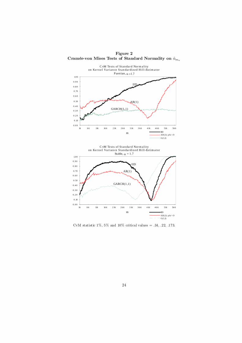
Figure 2Cramér-von Mises Tests of Standard Normality on

C vM Te sts of Standard Norm ali tyon Ke rne l Variance Standardiz e d Hil l -Estim ator

Paret ian,

IID

AR(1)

GARCH(1,1)

0 .0 0

0 .10

0 .2 0

0 .3 0

0 .4 0

0 .50

0 .6 0

0 .70

0 .8 0

0 .9 0

1.0 0

16 6 6 116 16 6 2 16 2 6 6 3 16 3 6 6 4 16 4 6 6 516 56 6

m IIDAR (1): p hi =.9

G(1,1)

C vM Te sts of Standard Normal ityon Ke rne l Variance Standardiz e d Hi l l -Estim ator

Stable, = 1.7

IID

AR(1)

GARCH(1,1)

0 .0 0

0 .10

0 .2 0

0 .3 0

0 .4 0

0 .50

0 .6 0

0 .70

0 .8 0

0 .9 0

1.0 0

16 6 6 116 16 6 2 16 2 6 6 3 16 3 6 6 4 16 4 6 6 516 56 6

m IIDAR (1): p hi =.9G(1,1)

CvM statistic 1%, 5% and 10% critical values = .34, .22, .173.

24

Figure 3NASDAQ and S&P500 Daily Log-Returns

NASDAQDailyReturns

-0.10

-0.08

-0.06

-0.04

-0.02

0.00

0.02

0.04

0.06

0.08

0.10

0.12

Jan-01 May-01 Oct-01 Mar-02 Aug-02 Jan-03 May-03

SP500DailyReturns

-0.04

-0.03

-0.02

-0.01

0.00

0.01

0.02

0.03

0.04

0.05

Jan-01 May-01 Oct-01 Mar-02 Aug-02 Jan-03 May-03

NASDAQHill-Estimator andRobustConfidenceBands

0

1

2

3

4

5

15 65 115 165 215 265 315 365 415 465 515 565 615 665

m a(m) a(m)-k a(m)+k

SP500Hill-Estimator andRobust Confidence Bands

0

1

2

3

4

5

15 65 115 165 215 265 315 365 415 465 515 565 615 665

m a(m) a(m)-k a(m)+k

NASDAQTwo-TailedTail Dependence Coefficient r(1)

andRobust Confidence Band

-0.30

-0.25

-0.20

-0.15

-0.10

-0.05

0.00

0.05

0.10

0.15

0.20

0.25

0.30

0.01 0.06 0.11 0.16 0.21 0.26 0.31 0.36 0.41 0.46 0.51 0.56 0.61 0.66

m/nth quantile-k r(1,m) k

SP500Two-TailedTail Dependence Coefficient r(1)

andRobust Confidence Band

-0.30

-0.25

-0.20

-0.15

-0.10

-0.05

0.00

0.05

0.10

0.15

0.20

0.25

0.30

15 65 115 165 215 265 315 365 415 465 515 565 615 665

m -k r(1,m) k

Notes: The median two-tailed tail dependence coe¢cients (1) over all m areNASDAQ: .10 § .07, and SP500: .17 § .09. As long as each fractile mbelongs to a sequence in S , the set of all proportional sequences,the median dependence coe¢cient is consistent and asymptoticallynormal under Assumptions A-C. See Hill (2006) for related theory andcomputation of the above plotted consistent kernel con…dence bands.

25

Figure 4

NASDAQInve rte d Hi l l -Estim ator,

Bias C orre cte d Inve rte d Hil l -Estim ator and Bias

-0 .2

-0 .1

0 .0

0 .1

0 .2

0 .3

0 .4

0 .5

0 .6

0 .7

0 .8

18 6 8 118 16 8 2 18 2 6 8 3 18 3 6 8 4 18 4 6 8

m

0

10

2 0

3 0

4 0

50

6 0

70

8 0

9 0

10 0

1/alp ha 1/alp ha(B )

B IAS M SE

SP500Inve rte d Hil l -Estim ator,

Bias C orre cte d Inve rte d Hi l l -Estim ator an d Bias

-0 .1

0 .0

0 .1

0 .2

0 .3

0 .4

0 .5

0 .6

18 6 8 118 16 8 2 18 2 6 8 3 18 3 6 8 4 18 4 6 8

m

0

10 0

2 0 0

3 0 0

4 0 0

50 0

6 0 0

70 0

8 0 0

9 0 0

10 0 0

1/alp ha 1/alp ha(B )

B IAS M SE

26

Table 1.1: Stable, = 17= 1000AR(1) G(1,1)

0 .2 .6 .9m § § § § §20 2.36§2.3 2.32§2.5 1.38§1.3 5.14§4.4 2.17§2.450 2.73§2.1 2.38§1.4 1.42§.98 2.41§2.0 2.02§1.8

100 2.05§.73 2.41§1.3 1.55§.84 3.60§1.8 1.95§.83150 2.32§.64 2.42§1.3 1.91§.80 3.21§1.3 2.03§.71200 2.15§.39 2.19§.45 2.11§.66 2.88§.79 1.97§.42300 1.89§.26 1.92§.31 1.89§.43 2.26§.48 1.81§.32400 1.69§.16 1.71§.24 1.79§.30 1.72§.40 1.62§.23500 1.47§.13 1.61§.15 1.48§.22 1.54§.20 1.41§.16

m¯ 2 369 381 411 422 347

m 460 477 518 510 454b~400 1.80 2.41 3.09 4.04 2.35400

KS05 415-430 420-435 422-445 390-440 310-380KS10 390-460 400-445 405-470 350-470 260-410

Notes: a. GARCH(1,1)b. Bandwidth = 1.96£b~/12

c. Minimum at which 2 does not occur in the 90% interval.d. Maximum at which = 1.7 occurs in the 95% interval.e. KS: Fractile range over which the Kolmogov-Smirnov test of normality

on 12 (-)/b~ is not rejected at the -level.

f. Excluding Paretian iid and GARCH data, in all cases the Cramér-von Misesstatistic is bi-modal over the fractile range. We only display the upper rangeof fractile values at which we fail to reject normality. See Figure 2.

Table 1.2: Minimum MSE EstimatesAR(1) G(1,1)

0 .2 .6 .9

¤ § ¤

1.66§.165 1.67§.202 1.63§.222 1.62§.274 1.77§.301¤

f2g 443 462 517 444 318 (.83)

¤ § ¤

1.87§.319 2.34§.117 1.84§.183 1.69§.202 1.76§.386¤

f2

()g 331 565 540 496 297 (.82)

Notes: a. Non-"bias corrected" ¤f2

g = arg min2f2

g.

b. "Bias corrected" ¤f2

()g = arg min2f2

()g.

27

Table 2.1: Paretian, = 17, = 1000AR(1) G(1,1)

0 .2 .6 .9m § § § § §20 1.83§1.15 1.85§1.20 2.14§1.53 3.18§2.62 2.09§2.150 1.79§.703 1.87§.783 2.04§.962 2.81§.146 1.88§1.7

100 1.85§.509 1.90§.584 2.12§.799 2.59§1.11 1.61§.72150 1.89§.421 1.95§.485 2.15§.662 2.46§.842 1.59§.57200 1.94§.372 1.99§.428 2.17§.573 2.32§.670 1.58§.39300 2.00§.308 2.08§.360 2.08§.427 2.05§.453 1.61§.32400 2.06§.268 2.13§.311 1.87§.302 1.78§.317 1.64§.28500 2.11§.239 2.14§.270 1.61§.208 1.52§.221 1.65§.25550 2.13§.228 2.13§.254 1.47§.180 1.39§.206 1.69§.31

m¯ 2 - - 448 423 180

m - - 536 510 575b~400 2.73 3.17 3.08 3.23 2.5950

KS05 15-48 15-50 430-485 400-450 15-85KS10 15-110 15-95 430-500 360-480 15-575

Notes: The "Paretian Tail" is P(Xz) = z¡(1 + z¡).

Table 2.2: Minimum MSE EstimatesAR(1) G(1,1)

0 .2 .6 .9

¤ § ¤

1.78§.684 1.74§.796 1.63§.254 1.62§.264 1.59§.743¤

f2g 51 46 452 446 48 (.56)

¤ § ¤

1.81§.674 1.66§.810 1.67§.245 1.63§.208 1.60§.327¤f2

()g 56 46 496 484 355 (.85)

Table 4. Equity Mininimum MSE EstimatesNASDAQ SP500

¤ § ¤

1.71§.204 2.02§.257¤

(2) =¤

(2()) 466 473

Notes: Sample size = 1422.

28