KERMACK{McKENDRICK EPIDEMIC MODEL REVISITED · Kermack{McKendrick Epidemic Model Revisited 397 If...

KYBERNET IK A — VOLUME 4 3 ( 2 0 0 7 ) , NU MB ER 4 , P AG E S 3 9 5 – 4 1 4

KERMACK–McKENDRICK EPIDEMIC MODELREVISITED

Josef Stepan and Daniel Hlubinka

This paper proposes a stochastic diffusion model for the spread of a susceptible-infective-removed Kermack–McKendric epidemic (M1) in a population which size is a martingale Nt

that solves the Engelbert–Schmidt stochastic differential equation (2). The model is givenby the stochastic differential equation (M2) or equivalently by the ordinary differentialequation (M3) whose coefficients depend on the size Nt. Theorems on a unique strong andweak existence of the solution to (M2) are proved and computer simulations performed.

Keywords: SIR epidemic models, stochastic differential equations, weak solution, simula-tion

Mathematics Subject Classification: 37N25, 60H10, 60H35, 92D25

1. INTRODUCTION

An epidemy of a highly infectious disease with a fast recovery (or fatality) in a homo-geneous population is considered, the influenza being an example of such epidemics.This classical Kermack–McKendrick model [12] assumes a fixed sized population ofn individuals, the population being divided into three subpopulations which changetheir respective sizes in the running time of the epidemic: Susceptibles (the individ-uals exposed to the infection), infectives (the infected individuals that are able tospread the disease) and removals (the individuals restored to health not able furtherto spread the infection or get themselves to be infected again) numbering by x(t),y(t) and z(t) the individuals that are susceptible, infected and removed at some timet ≥ 0, respectively. Hence, x(t) + y(t) + z(t) = n, x(t) and z(t) being generally anonincreasing and nondecreasing function, respectively such that z(0) = 0.

The model assumes the dynamics given by the following three dimensional dif-ferential equation

x(t) = −βx(t)y(t), x(0) = x0 > 0,

y(t) = βx(t)y(t)− γy(t), y(0) = y0 = n− x0 > 0, (M1)z(t) = γy(t), z(0) = 0,

396 J. STEPAN AND D. HLUBINKA

where the intensity β > 0 is higher for more infectious diseases and the parameterγ−1 > 0 is proportional to the average duration of the “being infected” status, i. e.to the average time for which an individual is infected.

In general there is no explicit solution to (M1), the approximation e−u ∼ 1−u+12u2 is known, (see [7]) to deliver a unique solution z as

z(t) ∼ ρ2

x0

(x0

ρ− 1

)+

αρ2

x0tanh

(12γαt− ϕ

)(S1)

with

α =

[2x0

ρ2(n− x0) +

(x0

ρ− 1

)2]1/2

(1)

ϕ = tanh−1

[1α

(x0

ρ− 1

)]

where ρ = γ/β denotes the relative removal rate of the disease. In some cases we mayget a precise solution assuming a non constant intensity β = β(x, y, z) or adopting amore simple and still realistic choice β = β(z). Assuming, for example, that β(z) ≥ 0is a decreasing function we in fact propose a model in which the population grows tobe more cautious and hence the epidemy will slow down its spread. See Theorem 1and the examples that follow.

Our aim is to propose and justify a diffusion version of (M1) model that allowsboth more general intensities β and to model the spread of epidemic in a populationthat changes its size Nt due to a diffusion type emigration and immigration processesdefined for example by the Engelbert–Schmidt stochastic differential equation

dNt = Ntσ(Nt) dWt, N0 = n0 := x0 + y0. (2)

If this is the case we assume

σ ≥ 0 bounded such that supp(σ) ⊂ [a, b], where 0 ≤ a ≤ n0 ≤ b < ∞, (3)

which assumption keeps the size of population Nt in the interval [a, b]. Furtherwe assume the ratios x(t), y(t) and z(t) of susceptibles, infectives and removals,respectively, to derive their dynamics from a generalized (M1) model that is givenas the ordinary differential equation with random time dependent coefficients

x(t) = −α(x(t), y(t), z(t), Nt) · x(t)y(t), x(0) =x0

n0

y(t) = α(x(t), y(t), z(t), Nt) · x(t)y(t)− γ · y(t), y(0) =y0

n0, (M3)

z(t) = γy(t), z(0) = 0,

(note that x(t) + y(t) + z(t) = 1), where α(x, y, z, n) is a function that is Lipschitzcontinuous on

(x, y, z) ∈ [0, 1]3, x + y + z = 1

uniformly for n ∈ [a, b].

Kermack–McKendrick Epidemic Model Revisited 397

If this is the case we are able to represent uniquely (Theorem 5 and Corollary 1) thesize Xt = x(t) ·Nt, Yt = y(t) ·Nt and Zt = z(t) · Nt of suspectibles, infectives andremovals, respectively, as the solution to a three dimensional SDE

dXt = −β(Xt, Yt, Zt)XtYt dt + Xtσ(Nt) dWt, X0 = x0 > 0dYt = β(Xt, Yt, Zt)XtYt dt− γYt dt + Ytσ(Nt) dWt, Y0 = y0 > 0 (M2)dZt = γYt dt + Z(t)σ(Nt) dWt, Z0 = 0,

where the intensities α(x, y, z, n) and β(x, y, z) rescale each other as α(x, y, z, n) =n ·β(nx, ny, nz). Note that the size of population Nt = Xt +Yt +Zt where (X,Y, Z)solves (M2) is a solution to (2). Theorems 2, 5 and Corollary 2 offer sufficient con-ditions for (M2) to have a unique strong and weak solution, respectively. Section 1,namely Theorem 1, summarizes and extends well-known properties of the solutionto the deterministic model (M1) and also possible choices of the intensity β(z) arelisted. The article is closed by Example 5 that delivers a visible computer illustrationof the above results.

We refer the reader to [4, 7], and to more recent [8] and [3] for the history andpresent state of art of stochastic modelling of epidemics.

The martingale and diffusion models probably first appeared in [6] where (inour setting and notation) the stochastic process Mt := Yt −

∫ t

0(βXuYu − γYu) du

is assumed to be a martingale which assumption makes it possible to estimate theconstant intensity β.

References [1, 2, 13, 14] propose a multidimensional diffusion model built upon the top of the deterministic infection in a population that consists only of sus-pectibles and infectives: Having interpreted γ as the disease death rate and β asits transmission rate, denoting by Nt = Xt + Yt the size of the population we maysimplify this model to the dimension one as

Xt = − β

NtXtYt, Yt =

β

NtXtYt − γYt, hence Nt = −γYt.

The authors propose its diffusion version given by the non-linear stochastic differ-ential equation

dXt = −βXtYt

Ntdt + b11(t) dW 1

t + b12(t) dW 2t ,

dYt = βXtYt

Ntdt− γYt dt + b21(t) dW 1

t + b22(t) dW 2t ,

where (W 1,W 2) is a two-dimensional standard Wiener process and

B = B(X,Y ) =

(b11 b12

b21 b22

)=

(βN XY − β

N XY

− βN XY β

N XY + γY

) 12

.

Phillips–Saranson theorem [16, 12.12 Theorem, p. 134] proves that the equation hasa unique strong solution and authors perform its sophisticated and instructive sim-ulations. Note that the size of population Nt is a supermartingale in this case.


Obviously, while the (M2) model expects an epidemic or even a pandemic with onlynegligible fatal consequences, the model proposed by [2] may be relevant when theinfections as HIV–AIDS in humans are studied.

[19] proved a unique existence theorem for a differential equation that, if gener-alized to R3, would cover the equation (M3).

2. KERMACK–McKENDRIC DETERMINISTIC EPIDEMIC

Here we shall treat (M1) deterministic model with an intenzity β = β(z) whichvalues are subject to changes dependent on the size of the removals subpopulation.Information on a solution (x(t), y(t), z(t)) to (M1) we are able recover in this case issummarized by

Theorem 1. Consider γ > 0 and assume β = β(z) to be a nonnegative, boundedand locally Lipschitz continuous function on R+. Then (M1) has a unique solution(x, y, z) ∈ C1(R+, R3) that is positive on (0,∞) and such that

x = X(z), y = Y (z) and z = γ[n− z −X(z)], z(0) = 0, (4)

hold, where

X(z) = x0 exp− 1

γ

∫ z

0

β(u) du

and Y (z) = n− z −X(z), 0 ≤ z ≤ n. (5)

The number of susceptibles individuals x(t) and the number of removals z(t) is apositive nonincreasing and increasing function on R+, respectively, such that 0 <x(∞) < n and 0 < z(∞) ≤ n while y(∞) exists and equals to zero.

The limit z(∞) is a solution to the equation

n− z = X(z) (6)

and if β(z) is nonincreasing on R+ then it is a unique solution to the equation onthe interval [0, n].

If β(0) > 0, γβ(0) < x0 and β(z) is again a nonincreasing function then the number

of infectives has a unique maximum y+ = y(t+), where

y+ = n− z+ −γ

β(z+), t+ =

1γ

∫ z+

0

1Y (u)

du (7)

and z+ is a unique 0 < z < z(∞) such that

β(z)X(z) = γ. (8)

The number of infectives y(t) is increasing on [0, t+] and decreasing on the interval[t+,∞].

All the above statements are proved for a constant β(z) in [7], for example.


P r o o f . The unique existence part follows from a more general Theorem 3 choos-ing there σ = 0. Also, apply (12), (13) and (14) in Lemma 1 to verify (4) and that(x, y, z) > 0 on (0,∞), hence (x, y, z) ∈ [0, n]3 on R+. It follows that z = γy > 0,hence z is an increasing function on R+ with z(∞) ∈ (0, n]. Similarly x ≤ 0 andx is seen as nonincreasing on R+ with n > x0 ≥ x(∞) = X(z(∞)) > 0. Thus,y(t) = n − x(t) − z(t) has a finite limit y(∞). Assuming y(∞) > 0 we concludethat limt→∞ z(t) > 0 which implies z(∞) = ∞, hence a contradiction. Finally,z(∞) = n− x(∞) < n.

The limit z(∞) solves (6) because n−z(∞) = x(∞) = X(z(∞)), according to (4).Assuming that β(z) is a nonincreasing function we get X(z) to be convex on R+.

Hence if 0 < z1 < z2 ≤ n are two distinct solutions to (6), then the graph of X(z) on[0, z2] is bellow the segment that connects the points (0, x0) and (z2, n− z2), whichsegment is further strictly bellow the segment that joins points (0, n) and (z2, n−z2).It follows that n− z1 > X(z1) which is a contradiction.

Compute

Y ′(z) = −1 +β(z)

γX(z), and Y ′(0+) = −1 +

β(0)γ

x0 > 0. (9)

It follows that there is a z ∈ (0, z(∞)) such that Y ′(z) = 0 as Y (0) = y0 > 0and Y (z(∞)) = 0. Assuming that Y ′(z1) = Y ′(z2) = 0 for a pair 0 < z1 < z2 <z(∞), or equivalently that (7) has not a unique solution in (0, z(∞)), it follows that1/X(z1) = β(z1)/γ ≥ β(z2)/γ = 1/X(z2). This and the inequality X(z1) ≥ X(z2)imply that X(z1) = X(z2) and further that β(z) = 0 on [z1, z2]. Hence, 1

X(z1)= 0

that contradicts the definition of X(z). Thus, there is unique z+ ∈ (0, z(∞)) suchthat −1 + β(z+)

γ X(z+) = Y ′(z+) = 0 and Y (z) increases and decreases on (0, z+)and (z+, z(∞)), respectively, Y (z+) being its unique maximum.

Finally, let t = t(z) be the inverse function to z = z(t). It follows by (M1) thatdtdz = 1

γY (z) , hence t(z) = 1γ

∫ z

01

Y (u) du and t+ = 1γ

∫ z+

01

Y (u) du is the only argumentof maxt<∞ y(t) = Y (z+). ¤

Remark 1. The number of removals z(t) is a unique solution to the differentialequation (4). Having computed the integral

t = t(z) =1γ

∫ z

0

[n− u− x0 exp

− 1

γ

∫ u

0

β(v) dv

]−1

du, (10)

and putting z(t) = t−1(z) we get the solution to (4).

Remark 2. The size of relative removal rate ρ = γ/β is considered by epidemiol-ogists as a good measure of the virulence of an epidemic: If x0 exceeds ρ only by asmall quantity then we model something as the common cold or a weak influenza.On the other hand, its values ρ ∼ x0/2 indicate the danger of a pandemic spread ofinfection.


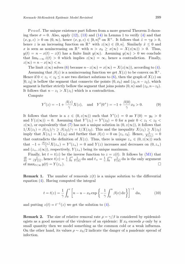
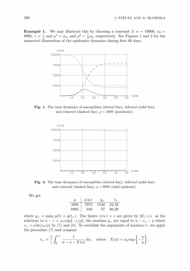
Example 1. We may illustrate this by choosing a constant β, n = 10000, x0 =9995, γ = 1

3 and ρ1 ∼ x0, and ρ2 ∼ 12x0, respectively. See Figures 1 and 2 for the

numerical illustration of the epidemics dynamics during first 60 days.

10 20 30 40 50 60time

2500

5000

7500

10000

size

Fig. 1. The time dynamics of susceptibles (dotted line), infected (solid line)

and removed (dashed line), ρ = 4995 (pandemic).

10 20 30 40 50 60time

2500

5000

7500

10000

size


and removed (dashed line), ρ = 8995 (mild epidemic).

We getρ z(∞) y+ t+

4995 7975 1540 22.338995 948 57 98.29

where y+ = maxt y(t) = y(t+). The limits z(∞) = z are given by (6), i. e. as thesolutions to n − z = x0 exp−z/ρ, the maxima y+ are equal to n − z+ − ρ wherez+ = ρ ln(x0/ρ) by (7) and (8). To establish the arguments of maxima t+ we applythe procedure (7) and compute

t+ =1γ

∫ z+

0

1n− u−X(u)

du, where X(u) = x0 exp−u

ρ

.


We have used program [9] in Mathematicar for numerical calculation (and interpo-lation) of x(·), y(·), z(·) and t+.

Remark 3. Having postulated that

β(z) ≥ 0 is a nonincreasing function supported by a compact [0, z1],

where z1 > 0 and such thatγ

β(0)< x0,

we assume that the intensity of infection monotonously decreases with the increasingnumber of removals and becomes negligible at the time t1 when z(t1) = z1. Notethat ρ(0) = γ/β(0) < x0 if and only if y(0+) > 0, and the latter inequality is acondition necessary and sufficient for the outbreak of the epidemic. Also note thatthe number of susceptibles x(t) = X(z(t)) is decreasing on [0, t1] and then remainsat the level x(t1) = X(z1) for ever. The number of removals will be of course stillincreasing to z(∞) = n−X(z1) ≥ z1.

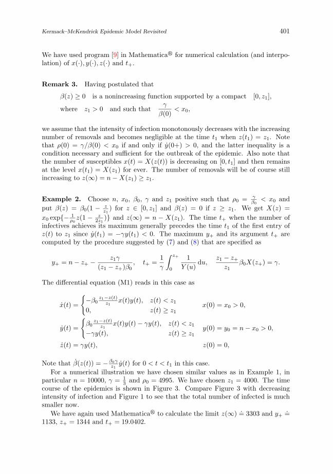
Example 2. Choose n, x0, β0, γ and z1 positive such that ρ0 = γβ0

< x0 andput β(z) = β0(1 − z

z1) for z ∈ [0, z1] and β(z) = 0 if z ≥ z1. We get X(z) =

x0 exp− 1ρ0

z(1 − z2z1

) and z(∞) = n − X(z1). The time t+ when the number ofinfectives achieves its maximum generally precedes the time t1 of the first entry ofz(t) to z1 since y(t1) = −γy(t1) < 0. The maximum y+ and its argument t+ arecomputed by the procedure suggested by (7) and (8) that are specified as

y+ = n− z+ −z1γ

(z1 − z+)β0, t+ =

1γ

∫ z+

0

1Y (u)

du,z1 − z+

z1β0X(z+) = γ.

The differential equation (M1) reads in this case as

x(t) =

−β0

z1−z(t)z1

x(t)y(t), z(t) < z1

0, z(t) ≥ z1

x(0) = x0 > 0,

y(t) =

β0

z1−z(t)z1

x(t)y(t)− γy(t), z(t) < z1

−γy(t), z(t) ≥ z1

y(0) = y0 = n− x0 > 0,

z(t) = γy(t), z(0) = 0,

Note that β(z(t)) = −β0γz1

y(t) for 0 < t < t1 in this case.For a numerical illustration we have chosen similar values as in Example 1, in

particular n = 10000, γ = 13 and ρ0 = 4995. We have chosen z1 = 4000. The time

course of the epidemics is shown in Figure 3. Compare Figure 3 with decreasingintensity of infection and Figure 1 to see that the total number of infected is muchsmaller now.

We have again used Mathematicar to calculate the limit z(∞) .= 3303 and y+.=

1133, z+ = 1344 and t+ = 19.0402.


10 20 30 40 50 60time

2500

5000

7500

10000

size


and removed (dashed line), β(z) decreasing function.

Example 3. Kendall [11] proposes (see also [7]) a more sophisticated choice forβ(z) in the form

β(z) =

2β0

(1−z/ρ0)+(1−z/ρ0)−1 , 0 ≤ z ≤ ρ0, ρ0 = γβ0

, γ, β0 > 0.

= 0, z ≥ ρ0,

Note that β(z) is chosen such that the assumptions of Remark 3 are satisfied, inparticular z1 = ρ0, β(0) = β0, and z(∞) = n−X(ρ0) = (x0/ρ− 1 + α)ρ2/x0, withα given by (1).

3. KERMACK–McKENDRICK WITH A STOCHASTIC EMIGRATIONAND IMMIGRATION

A random three dimensional dynamics Lt = (Xt, Yt, Zt), t > 0 of the numberXt, Yt and Zt of susceptibles, infectives and removals, respectively, with the sizeof population Nt = Xt + Yt + Zt whose stochastic nature is caused by small ran-dom emigration-immigration perturbations is proposed by the stochastic differentialequations (M2) where β(x, y, z) and σ(n) are suitable functions on R3 and R1, re-spectively. Note that the size Nt is a solution to the Engelbert–Schmidt stochasticdifferential equation (2). The nature of β(x, y, z), or perhaps more simply of β(z),and the constant γ > 0 that enter (M2) is explained in Section 1. The diffusioncoefficient σ(n) is designed to control the global size of the population Nt insidereasonable bounds. It can be seen, for example, by choosing σ(n) as in (3) sincea ≤ Nt ≤ b holds almost surely in this case. Note that choosing a = b = n0 andσ = 0 (M2) becomes (M1).

Let us agree that Lt = (Xt, Yt, Zt) is a solution to (M2) if (M2) makes sense andif it holds for a standard Brownian motion Wt defined on a complete probabilityspace (Ω,F , P ), i. e. if X, Y and Z are continuous Ft-semimartingales that satisfy(M2), having denoted by Ft the augmented canonical filtration of the process Wt.


Recall that (M2) is said to have a unique strong solution if there is an almost surelydetermined solution on arbitrary (Ω,F , P,W ). Also recall that (M2) is said to havea unique weak solution if there is a setting (Ω,F , P,W ) on which a solution X,Y, Zmay be constructed and if L(X,Y, Z) = L(X ′, Y ′, Z ′) whatever solutions to(M2)(X,Y, Z) and (X ′, Y ′, Z ′) might be chosen.

By Ito formula, or more precisely by [10, Proposition 21.2] on Doleans equation,we prove easily the following lemma.

Lemma 1. Assume β(z, y, z) and σ(n) bounded. Then (X,Y, Z) is a solution to(M2) if and only if

Nt = n0 exp∫ t

0

σ(Nu) dWu −12

∫ t

0

σ2(Nu) du

, (11)

Xt =x0

n0exp

−

∫ t

0

β(Xu, Yu, Zu)Yu du

·Nt, (12)

Yt =y0

n0exp

∫ t

0

β(Xu, Yu, Zu)Xu du− γt

·Nt, (13)

Zt = γ

∫ t

0

Yu

Nudu ·Nt (14)

hold for all t ≥ 0 almost surely. Especially, processes X,Y and N are positive onR+ and Z is a process positive on (0,∞).

Theorem 2. Assume β nonnegative and bounded, let σ satisfy (3) and considerarbitrary solution (X,Y, Z) to (M2). Then the following statements hold;

(i) The size of population Nt is a bounded martingale such that a ≤ N ≤ b holdsand such that the limit N∞ := lim

t→∞Nt exists. Especially, ENt = n0 holds for

all t ≥ 0.

(ii) If supp(σ) = (a, b) and∫ a+

a1

u2σ2(u) du =∫ b

b−1

u2σ2(u) du = ∞, the limit N∞equals to a and b with probability b−n0

b−a and n0−ab−a , respectively.

(iii) The number of susceptibles 0 < X ≤ b and the number of removals 0 ≤ Z ≤ bis a supermartingale and submartingale, respectively. The process Z is positiveon (0,∞). Especially, EXs ≥ EXt and EZs ≤ EZt holds for s ≤ t.

(iv) All limits X∞, Y∞ and Z∞ exist, Y∞ = 0 and X∞ > 0 if and only if N∞ > 0,hence assuming a > 0 we get X∞ as a positive random variable.

Observe that all the above statements, equalities and inequalities are meant tohold almost surely, for example X > 0 is to be read as Xt > 0 holds for all t ≥ 0almost surely. The stated martingale and semimartingale properties are w.r.t. theaugmented canonical filtration of Wt denoted by Ft. For example, the statement Xis a supermartingale is precisely as X is an Ft-supermartingale.


P r o o f . The size of population Nt is a positive local martingale by definitionand by (11). It is a constant on a bounded interval (s, t) if and only if its quadraticvariation [N ]t =

∫ t

0N(u)2σ2(Nu) du has the same property [16, 30.4 Theorem, p. 54].

Since [σ2 > 0] = (a, b) we reason that a ≤ N ≤ b and therefore Nt is a boundedmartingale. Thus, according to [15, Theorem 69.1, p. 176] a ≤ N∞ ≤ b exists. Wehave proved (i).

The proof of (ii) will be postponed until Theorem 5.Since Nt is a martingale and −

∫ t

0β(Xu, Yu, Zu)Yu du a nonincreasing process we

get 0 ≤ X ≤ b as a bounded supermartingale by (12) in Lemma 1. Similarly, weverify that 0 ≤ Zt ≤ b is a bounded submartingal by (14). This concludes the proofof (iii).

It follows by the supermartingale and submartingale property of bounded pro-cesses Xt and Zt, respectively, applying [15, Th. 69.1] again, that X∞ and Z∞ exist.To prove that Y∞ = N∞ − X∞ − Z∞ = 0 we shall verify that

∫∞0

Yu du < ∞:Observe first that

∫ t

0Z2

uσ2(Nu) du < ∞ holds for all t > 0. This implies that∫ t

0Zuσ(Nu) dWu defines an L2 -martingale. Hence, E

∫ t

0Yu du = 1

γ EZt by (M2) andE

∫∞0

Yu du = 1γ EZ∞ ≤ b

γ . In particular,∫∞0

Yu du < ∞. Finally, observing that∫∞0

β(Xu, Yu, Zu)Yu dy ≤ c∫∞0

Yu du < ∞ for a c ∈ (0,∞), it follows by (12) thatX∞ > 0 if and only if N∞ > 0 and (iv) is proved completely. ¤

A unique strong solution to (M2) exists under fairly mild requirements on thecoefficients β(x, y, z) and σ(n). Putting L = (X,Y, Z) we write (M2) as

dLt = b(Lt) dt + a(Lt) dBt, L0 = (x0, y0, 0), (15)where

b(x, y, z) =

b1(x, y, z)b2(x, y, z)b3(x, y, z)

=

−xyβ(x, y, z)xyβ(x, y, z)− γy

γy

: R3 → R3,

a(x, y, z) =

a11(x, y, z) 0 0a21(x, y, z) 0 0a31(x, y, y) 0 0

=

xσ(x + y + z) 0 0yσ(x + y + z) 0 0zσ(x + y + z) 0 0

: R3 → M3

and Bt = (W 1t ,W 2

t ,W 3t ) is a three dimensional Brownian motion with W 1

t = Wt.By M3 we have denoted the space of the 3×3-matrices endowed with the Eucleidiannorm. A standard of stochastic analysis [16, V.12.1 Theorem] says that (15) hasa unique strong solution provided that the maps b and a are locally Lipschitz andof a linear growth. Even though our particular case (M2) involves a coefficientb = (b1, b2, b3) that is not of a linear growth whatever nontrivial bounded β(x, y, z)may be chosen, we are able to prove

Theorem 3. Let σ(n) be a Lipschitz continuous function such that (3) holdsfor some a ≤ b. Further, assume that β(x, y, z) is a nonnegative function that isLipschitz continuous on

∆ab :=(x, y, z) ∈ [0, b]3, a ≤ x + y + z ≤ b

.


Then (M2) has a unique strong solution L = (X,Y, Z) that is a positive process on(0,∞) such that a ≤ N = X + Y + Z ≤ b.

P r o o f . Choose bounded locally Lipschitz ϕi(x, y, z) : R3 → R such that

ϕ1(x, y, z) = −β(x, y, z)y, ϕ2(x, y, z) := β(x, y, z)x holds for (x, y, z) ∈ ∆ab

and consider the stochastic differential equations

dXt = ϕ1(Xt, Yt, Zt)Xt dt + Xtσ(Nt) dWt, X0 = x0

dYt = ϕ2(Xt, Yt, Zt)Yt dt + Ytσ(Nt) dWt − γYt dt, Y0 = y0 (16)dZt = γYt dt + Ztσ(Nt) dWt, Z0 = 0,

where Nt = Xt + Yt + Zt. This is the case of equation (15) that has coefficientsb(x, y, z) and a(x, y, z) that are locally Lipschitz and of a linear growth. Hence,by [16, V.12.1 Theorem], (16) has a unique strong solution L = (X,Y, Z) that ispositive on (0,∞):

Xt =x0 exp∫ t

0

ϕ1(Xu, Yu, Zu)− 12σ2(Nu) du +

∫ t

0

σ(Nu) dWu

,

Yt =y0 exp∫ t

0

ϕ2(Xu, Yu, Zu)− 12σ2(Nu) du− γt +

∫ t

0

σ(Nu) dWu

,

andZt = exp

∫ t

0

σ(Nu) dWu −12

∫ t

0

σ2(Nu) du

×

∫ t

0

exp−

∫ u

0

σ(Nw) dWw +12

∫ u

0

σ2(Nw) dw

· γYu du

by [10, Theorem 21.2] again. Denote by τ := inft > 0 : Lt /∈ ∆ab the first entry ofL = (X,Y, Z) to the complement of ∆ab. Obviously, (16) yields equations

Xt∧τ = x0 +∫ t∧τ

0

−β(Xu, Yu, Zu)XuYu du +∫ t∧τ

0

Xuσ(Nu) dWu,

Yt∧τ = y0 +∫ t∧τ

0

β(Xu, Yu, Zu)XuYu − γYu du +∫ t∧τ

0

Yuσ(Nu) dWu (17)

Zt∧τ = γ

∫ t∧τ

0

Yu du +∫ t∧τ

0

Zuσ(Nu) dWu.

Hence, Nt = n0 +∫ t

0Nuσ(Nu) dWu for t ≤ τ and therefore a ≤ Nt ≤ b for any

such t as supp(σ) ⊂ [a, b]. Obviously there is no t > 0 for which either Nt /∈[a, b] or min(Xt, Yt, Zt) < 0 would hold, consequently there is no t > 0 such thatmax(Xt, Yt, Zt) > b. Hence τ = ∞. Reading (17) again we conclude that (X,Y, Z)solves (M2).

Finally, if (X,Y, Z) is a solution to (M2) it follows from Theorem 2 that (Xt, Yt, Zt)∈ ∆ab at any time t. It yields that (X,Y, Z) is a solution to (16). The stochasticdifferential equation (M2) has a unique strong solution since (16) has the property.

¤Later on we shall appreciate even a more general result.


Theorem 4. Consider (M2) model with a time dependent intensity β(x, y, z, t) ≥ 0that is Lipschitz continuous on ∆ab uniformly for t ≥ 0 (especially bounded on ∆ab).Also let a Lipschitz continuous σ(n) to satisfy (3) for some a ≤ b. Then (M2) has aunique strong solution and any solution L = (X,Y, Z) to (M2) is a positive processon (0,∞) with a ≤ N = X + Y + Z ≤ b.

The proof goes along the lines of the reasoning employed in the proof of of The-orem 3 only a finer construction of Lipschitz extensions ϕi has to be performed:Define ϕi : C(R+, R3)× R → R for t ≥ 0, (x., y., z.) ∈ C(R+, R3) by

ϕ1(x., y., z., t) = −β(xt∧τ , yt∧τ , zt∧τ , t ∧ τ) · yt∧τ

ϕ2(x., y., z., t) = β(xt∧τ , yt∧τ , zt∧τ , t ∧ τ) · xt∧τ ,

where τ = τ(x., y., z.) = inf t > 0 : (xt, yt, zt) /∈ ∆ab : C(R+, R3) → [0,∞] is timeof the first entry of the C(R+, R3)-canonical process lt = (xt, yt, zt) to the com-plement of ∆ab. It easy to check that ϕ1 and ϕ2 are bounded progressive pathfunctionals on C(R+, R3) × R+ that are Lipschitz continuous on C(R+, R3), i. e.such that

|ϕi(l·, t)− ϕi(l′·, t)| ≤ C · ‖l − l′‖t, l, l′ ∈ C(R+, R3), t ≥ 0 (18)

holds for a constant C and ‖l‖t denotes the sup-norm in C([0, t], R3). Putting

b(l·, t) =

ϕ1(l·, t)xt

ϕ2(l·, t)yt − γyt

γyt

, a(l·, t) =

xtσ(xt + yt + zt) 0 0ytσ(xt + yt + zt) 0 0ztσ(xt + yt + zt) 0 0

for lt = (xt, yt, zt) ∈ C(R+, R3) and t ≥ 0 we propose a three dimensional SDE

dLt = b(Lt, t) dt + a(Lt, t) dBt, L0 = (x0, y0, 0) (19)

where Lt = (Xt, Yt, Zt) and Bt = (Wt,W2t ,W 3

t ) is a three dimensional standardBrownian motion as before. Because b and a are progressive path functionals

b : C(R+, R3)× R+ → R3, a : C(R+, R3)× R+ → M3

such that |b(l·, t)− b(l′·, t)|+ |a(l·, t)− a(l′·, t)| ≤ CN · ‖l − l′‖t,

holds for ‖l‖ ≤ N , ‖l′‖ ≤ N , N ∈ N and t ≥ 0 and

|b(l., t)|+ |a(l., t)| ≤ C · (1 + ‖l‖)

holds for all l ∈ C(R+, R3) and t ≥ 0 according to (18), where CN and C are con-stants. We have denoted by |b|, |a|, the Eucleidian norms in R3 and M3, respectivelyand ‖l‖ the sup-norm in C(R+, R3). It follows by [16, V.12.1 Theorem], p. 131 that(19) has a unique strong solution. Choosing a solution L = (X,Y, Z) to (19) we pro-ceed the proof exactly as in the proof of Theorem 3 putting there τ = τ(L) whereτ : C(R+, R3) → [0,∞] is defined as the first entry of l. to R3 \∆ab.


Remark 4. Saying that b(l., t) is a progressively measurable map we mean that bis an Ct-progressive process on C(R+, R3) where Ct is the minimal right continuousfiltration built up on the top of the canonical filtration Ht in C(R+, R3). It is easy tocheck that V.12.1 Theorem of [16], that is formulated for Ht-progressive (previsible)coefficients, is applicable more generally for the Ct-progressive path functionals aand b. Our reason for this enrichment is that τ , being a Ct-Markov time, lacks thisproperty with respect to the canonical filtration Ht.

4. WEAK SOLUTIONS TO KERMACK–McKENDRICK STOCHASTICEPIDEMIC MODEL

The following theorem suggests a two-step procedure for obtaining a solution (X,Y, Z)to (M2).

Theorem 5. A semimartingale Lt = (Xt, Yt, Zt) is a solution to (M2) if and only if

Xt = x(t) ·Nt, Yt = y(t) ·Nt, Zt = z(t) ·Nt, t ≥ 0, almost surely, (20)

where Nt is is a solution to Engelbert–Schmidt stochastic differential equation (2)and l(t) =

(x(t), y(t), z(t)

)is a semimartingale that solves almost surely the or-

dinary differential equation with random coefficients (M3) where α(x, y, z, n) =n · β(nx, ny, nz) for (x, y, z, n) ∈ R4.

P r o o f . Let L = (X,Y, Z) to solve (M2) and put l(t) = (x(t), y(t), z(t)) :=1

Nt(Xt, Yt, Zt) where N = X + Y + Z. Then Nt is a solution to (2) and it follows by

(12), (13) and (14) in Lemma 1 that (x(t), y(t), z(t)) is a solution to (M3) almostsurely.

On the other hand, consider a solution Nt to (2) and(x(t), y(t), z(t)

)a solution

to (M3). Note that x(t)+y(t)+z(t) = 1 and put (Xt, Yt, Zt) :=(x(t), y(t), z(t)

)·Nt.

It follows that

x(t) = x(0) · exp−

∫ t

0

α(x(u), y(u), z(u), Nu) · y(u) du

=x0

n0· exp

−

∫ t

0

β(Xu, Yu, Zu) · Yu du

,

y(t) = y(0) · exp∫ t

0

α(x(u), y(u), z(u), Nu) · x(u) du− γ · t

=y0

n0· exp

∫ t

0

β(Xu, Yu, Zu) ·Xu du− γt

andz(t) = γ

∫ t

0

y(u) du = γ

∫ t

0

Yu

Nudu,

that is exactly as to say that (Xt, Yt, Zt) is a solution to (M2) according to Lemma 1.¤


We need sufficient conditions for (M3) to have a unique solution almost surely.Observe the following requirements on β(x, y, z) and α(x, y, z, n), respectively.

(i) β(x, y, z) is a Lipschitz continuous function on ∆ab.

(ii) α(x, y, z, n) is Lipschitz continuous on ∆11 =(x, y, z) ∈ [0, 1]3, x + y + z = 1

uniformly for n ∈ [a, b].

(iii) For arbitrary N. ∈ C(R+) such that a ≤ N. ≤ b the function α(x, y, z,Nt) isLipschitz continuous on ∆11 uniformly for t ≥ 0.

(iv) For arbitrary N ∈ C(R+) such that a ≤ N ≤ b and N0 = n0, the equation(M3) has a unique solution l(N, t) = (x(N, t), y(N, t), z(N, t)) ∈ C(R+, R3).

It is obvious that

(i) =⇒ (ii) =⇒ (iii) =⇒ (iv), (21)

where the last implication is proved by Theorem 4 with a = b = 1, especially withσ = 0. Consequently, the proposed two-step construction of a solution to (M2) isgood one from the mathematical point of view.

Corollary 1. Let either β(x, y, z) to satisfy (i) or α(x, y, z, n) to satisfy (ii) andassume that σ(n) follows (3) for some a ≤ b. Then (M2) has a unique strong solutionif and only if the equation (2) has the property. Moreover, assuming that (2) has aunique weak solution (M2) inherits the property.

P r o o f . The first assertion is mostly a simple consequence of Theorem 5 applyingthe chain of implications (21). It remains to assume that (M2) has a unique strongsolution and prove that N = N ′ almost surely for any pair of solutions to (2).Let l(t) = (x(t), y(t), z(t)) be the unique solution to (M3) generated by Nt andl′(t) = (x′(t), y′(t), z′(t)) the unique solution to (M3) generated by N ′

t . Then l(t) ·Nt = l′(t)N ′

t holds for t ≥ 0 almost surely. Hence, N ′t = c(t) ·Nt, where c(t) := x(t)

x′(t) ,c(0) = 1, is a continuous process of finite variation. Since Nt is a martingale, itfollows by Ito per partes formula that E

∫ t

0Nu dc(u) = 0 for all t ≥ 0 almost surely,

hence c is a process with constant trajectories. Thus, c(t) = 1 for all t and thereforeN = N ′.

Note that (iv) defines a map

F :N ∈ C(R+), a ≤ N ≤ b, N0 = n0

→ C(R+, R3)

that sends any such N to F (N)(t) = l(N, t), i. e. to a unique solution to (M3)generated by N . The map F is easily seen to be Borel measurable and thereforethe probability distribution of Nt uniquely determines the probability distributionof N · F (N) that is a solution to (M2) according to Theorem 5. ¤

We suspect that there might be situations when (M2) has a unique weak solutionwhile there need not to exist a unique strong solution to the Engelbert–Schmidtequation (2).


Example 4. Choose β(x, y, z) such that β(x, y, z) = BA(x+y+z)+z holds on ∆ab.

Then α(x, y, z, n) = BA+z is Lipschitz on ∆11 and the equation (M3) adopts the

deterministic form of Kermack–McKendric model scrutinized in Theorem 1.

Write p0 = x0/n0 and q0 = y0/n0 = 1− p0. We get (M1) as

x = − B

A + z· x · y, x(0) = p0

y =B

A + z· x · y − γy, y(0) = q0

z = γ · y, z(0) = 0.

We easily compute

X(z) = p0 · exp− 1

γ

∫ z

0

α(u) du

= p0

(A

A + z

)B/γ

andY (z) = 1− z − p0

(A

A + z

)B/γ

.

Choosing B = γ and A = p02 we get γ

α(0) = A < p0 and observe that Theorem 1 isapplicable completely with

α(z) =2γ

p0 + 2z, X(z) =

p20

p0 + 2zand Y (z) = 1− z − p2

0

p0 + 2z.

The above differential equation has a unique solution (x(t), y(t), z(t)) on R+, z(t)being computed by solving

z = γ ·(

1− z − p20

p0 + 2z

), z(0) = 0.

There is no explicit solution to this differential equation nevertheless some featuresof the solution can be stated. The limit z∞ = limt→∞ z(t) ∈ [0, 1] may be computedby solving 1− z∞ = X(z∞) = p2

0/(p0 + 2z∞). We get

z∞ =2− p0 +

√4 + 4p0 − 7p2

0

4, x∞ =

2 + p0 −√

4 + 4p0 − 7p20

4.

Also solve the equation 2p20 = (p0 + 2z+)2 to establish a z+ ∈ (0,∞) and compute

y+ = 1− z+ −p20

p0 + 2z+, t+ =

1γ

∫ z+

0

21− u− p2

0(p0 + 2u)−1du

to get

y+ = max y(t) = 1− p0

(√2− 1

2

), z+ = p0

√2− 12

, x+ = p0

√2

2

and t+ > 0 such that y+ = y(t+).


We summarize that having (M2) model with β(x, y, z) = 2γp0(x+y+z)+2z and a

Lipschitz continuous function σ(n) that satisfies (10) for a pair a ≤ b, we get amodel that has a unique strong solution

Xt = x(t) ·Nt, Yt = y(t) ·Nt, zt = z(t) ·Nt,

where Nt solves the equation (2). We easily compute that

EXt = x(t) · n0, EYt = y(t) · n0, EZt = z(t) · n0.

The above two-step procedure obviously generates a couple of problems:

(A) To solve Engelbert–Schmidt equation (10) by which we mean to receive aninformation as complex as possible about the probability distribution of itssolution Nt with the aim to deliver simulations of its trajectories and formulasfor the moments ENk

t . To complicate things even more epidemiologists prefermodels with possibly non-Lipschitz weight functions σ(n)

σ(n) = K(n− a)µ · (b− n)ν , a ≤ n ≤ b, 0 < a < n0 < b < ∞, µ, ν > 0.

(B) Having done this we are of course expected to solve the ordinary equation (M3)with the similar aims as proposed by (A).

To this end precise requirements (2) as

σ ≥ 0 bounded with supp(σ) = (a, b), 0 < a < n0 < b < ∞, (22)∫ a+

a

1n2σ2(n)

dn =∫ b

b−

1n2σ2(n)

dn = ∞ (23)

and note that (23) is satisfied for Lipschitz continuous σ(n) that satisfy (22). Con-sider a Brownian motion B(t) such that B(0) = n0, denote

A(s) =∫ s

0

1B(u)2σ2(B(u))

du, s ≥ 0, τt = inf s > 0 : A(s) > t , t ≥ 0

and recall Engelbert–Schmidt Theorem [10, Theorem 23.1, Lemma 23.2, p. 451–2] toget (looking also through the proofs) a simple

Corollary 2. Assume (22). Then the condition (23) is necessary and sufficient forthe equation (2) to have a unique weak solution. Arbitrary solution Nt to (2) isequally distributed in C(R+) as the continuous stochastic process B(τt). Moreover,

τ∞ := inf s ≥ 0 : A(s) = ∞ = limt→∞

τt = inf s ≥ 0 : B(s) ∈ a, b . (24)

In a combination with Corollary 1 we also prove


Corollary 3. Assume (22) and (23) for σ(n) and consider arbitrary α(x, y, z, n) =n · β(nx, ny, nz) that is Lipschitz continuous on

∆11 =(x, y, z) ∈ [0, 1]3 : x + y + z = 1

uniformly for n ∈ [a, b]. Then the equation (M2) has a unique weak solution.

Engelbert–Schmidt Theorem in a more detailed form of Corollary 2 also provesthe (ii) statement in Theorem 2:

Consider arbitrary solution Nt to the equation (2). It follows by (24) that the limitN∞ and transformation B(τ∞) are equally distributed random variables. BecauseB(τ∞) is a a, b-valued random variable almost surely and τ∞ a Markov time suchthat B(t) ∈ [a, b] if τ∞ ≥ t we may apply the Wald equalities

aP[B(τ∞) = a]+b P[B(τ∞) = b] = n0, a2P[B(τ∞) = a]+b2P[B(τ∞) = b] = Eτ∞

to verify (ii) in Theorem 2.The reader may find in [17, 18] a source of information relevant to the problems

proposed by (A).

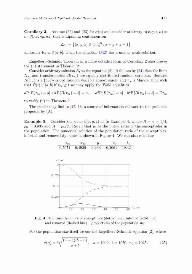
Example 5. Consider the same β(x, y, z) as in Example 4, where B = γ = 1/4,p0 = 0.995 and A = p0/2. Recall that p0 is the initial ratio of the susceptibles inthe population. The numerical solution of the population ratio of the susceptibles,infected and removed dynamics is shown in Figure 4. We can also calculate

z∞ x∞ y+ z+ t+0.5074 0.4926 0.0904 0.2061 19.42

.

10 20 30 40 50 60time

0.25

0.5

0.75

1

size


and removed (dashed line) – proportions of the population size.

For the population size itself we use the Engelbert–Schmidt equation (2), where

σ(n) = 6

√(n− a)(b− n)

a + b, a = 1000, b = 1050, n0 = 1025. (25)


10 20 30 40 50 60

1020

1025

1030

1035

1040

1045

1050

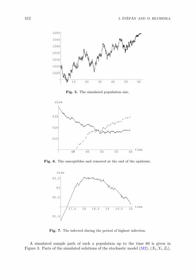
Fig. 5. The simulated population size.

40 45 50 55 60time

510

520

530

size

Fig. 6. The susceptibles and removed at the end of the epidemic.

17.5 18 18.5 19 19.5 20time

91.5

92.5

93

93.5

size

Fig. 7. The infected during the period of highest infection.

A simulated sample path of such a population up to the time 60 is given inFigure 3. Parts of the simulated solutions of the stochastic model (M2), (Xt, Yt, Zt),


are shown in Figures 6 and 7. The population dynamics is, however, quite smallwith respect to the dynamics of the size of susceptibles, infected and removed. Thepopulation size is between 1,000 and 1,050 to keep the emmigration/immigrationdynamics realistic. On the other hand the number of susceptibles changes from 995to 500 quite fast.

ACKNOWLEDGEMENT

This work was partially supported by the Ministry of Education, Youth and Sports of theCzech Republic under research project MSM 0021620839. The work of J.S. was partiallyfinanced by the Czech Science Foundation under grant 201/03/1027, the work of D.H. waspartially financed by the Czech Science Foundation under grant 201/03/p138.The authors thank for the interesting problem proposed to them by the Roche Company.

(Received April 18, 2006.)

REFERENC ES

[1] E. J. Allen: Stochastic differential equations and persistence time for two interactingpopulations. Dynamics of Continuous, Discrete and Impulsive Systems 5 (1999), 271–281.

[2] L. J. S. Allen and N. Kirupaharan: Asymptotic dynamics of deterministic and stochas-tic epidemic models with multiple pathogens. Internat. J. Num. Anal. Model. 2 (2005),329–344.

[3] H. Andersson and T. Britton: Stochastic Epidemic Models and Their Statistical Anal-ysis. (Lecture Notes in Statistics 151.) Springer–Verlag, New York 2000.

[4] N.T. J. Bailey: The Mathematical Theory of Epidemics. Hafner Publishing Comp.,New York 1957.

[5] F. Ball and P. O’Neill: A modification of the general stochastic epidemic motivatedby AIDS modelling. Adv. in Appl. Prob. 25 (1993), 39–62.

[6] N.G. Becker: Analysis of infectious disease data. Chapman and Hall, London 1989.[7] D. J. Daley and J. Gani: Epidemic Modelling; An Introduction. Cambridge University

Press, Cambridge 1999.[8] D. Greenhalgh: Stochastic Processes in Epidemic Modelling and Simulation. In: Hand-

book of Statistics 21 (D. N. Shanbhag and C.R. Rao, eds.), North–Holland, Amster-dam 2003, pp. 285–335.

[9] J. Hurt: Mathematicar program for Kermack–McKendrick model. Department ofProbability and Statistics, Charles University in Prague 2005.

[10] O. Kallenberg: Foundations of Modern Probability. Second edition. Springer–Verlag,New York 2002.

[11] D.G. Kendall: Deterministic and stochastic epidemics in closed population. In: Proc.Third Berkeley Symp. Math. Statist. Probab. 4, Univ. of California Press, Berkeley,Calif. 1956, pp. 149–165.

[12] W.O. Kermack and A.G. McKendrick: A contribution to the mathematical theory ofepidemics. Proc. Roy. Soc. London Ser. A 115 (1927), 700–721.

[13] N. Kirupaharan: Deterministic and Stochastic Epidemic Models with MultiplePathogens. PhD Thesis, Texas Tech. Univ., Lubbock 2003.

[14] N. Kirupaharan and L. J. S. Allen: Coexistence of multiple pathogen strains in stochas-tic epidemic models with density-dependent mortality. Bull. Math. Biol. 66 (2004),841–864.


[15] L. C.G. Rogers and D. Williams: Diffusions, Markov Processes and Martingales. Vol. 1:Foundations. Cambridge University Press, Cambridge 2000.

[16] L. C.G. Rogers and D. Williams: Diffusions, Markov Processes and Martingales. Vol. 2:Ito Calculus. Cambridge University Press, Cambridge 2000.

[17] J. Stepan and P. Dostal: The dX(t) = Xb(X)dt + Xσ(X) dW equation and financialmathematics I. Kybernetika 39 (2003), 653–680.

[18] J. Stepan and P. Dostal: The dX(t) = Xb(X)dt + Xσ(X)dW equation and financialmathematics II. Kybernetika 39 (2003), 681–701.

[19] R. Subramaniam, K. Balachandran, and J.K. Kim: Existence of solution of a stochas-tic integral equation with an application from the theory of epidemics. Nonlinear Funct.Anal. Appl. 5 (2000), 23–29.

Josef Stepan and Daniel Hlubinka, Department of Probability and Statistics, Faculty of

Mathematics and Physics – Charles University, Sokolovska 83, 186 75 Praha 8. Czech

Republic.

e-mails: [email protected], [email protected]

KERMACK{McKENDRICK EPIDEMIC MODEL REVISITED · Kermack{McKendrick Epidemic Model Revisited 397 If...

Documents

Transcript of KERMACK{McKENDRICK EPIDEMIC MODEL REVISITED · Kermack{McKendrick Epidemic Model Revisited 397 If...