Neuroinformatics 1: review of statistics Kenneth D. Harris UCL, 28/1/15.
Basic Statistics for Research
Kenneth M. Y. Leung
Why do we
need statistics?
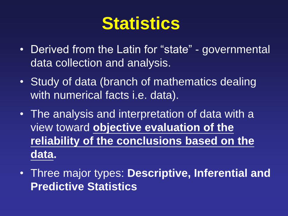
Statistics
• Derived from the Latin for “state” - governmental
data collection and analysis.
• Study of data (branch of mathematics dealing
with numerical facts i.e. data).
• The analysis and interpretation of data with a
view toward objective evaluation of the
reliability of the conclusions based on the
data.
• Three major types: Descriptive, Inferential and
Predictive Statistics
Variation - Why statistical
methods are needed
http://www.youtube.com/watch?v=fsRYkRqQqgg&feature=related
By UCMSCI
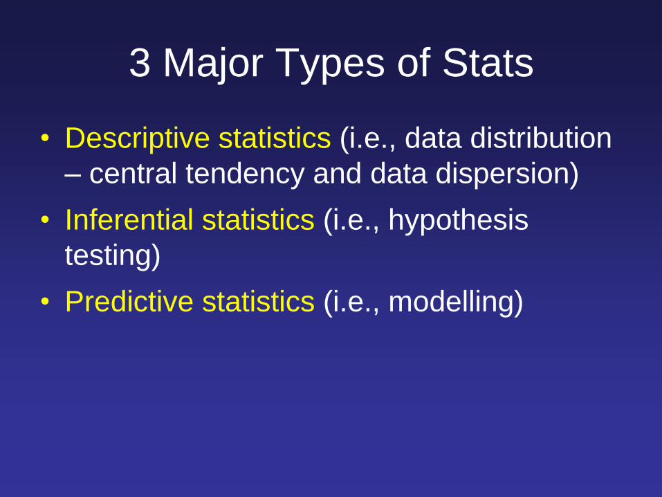
3 Major Types of Stats
• Descriptive statistics (i.e., data distribution
– central tendency and data dispersion)
• Inferential statistics (i.e., hypothesis
testing)
• Predictive statistics (i.e., modelling)
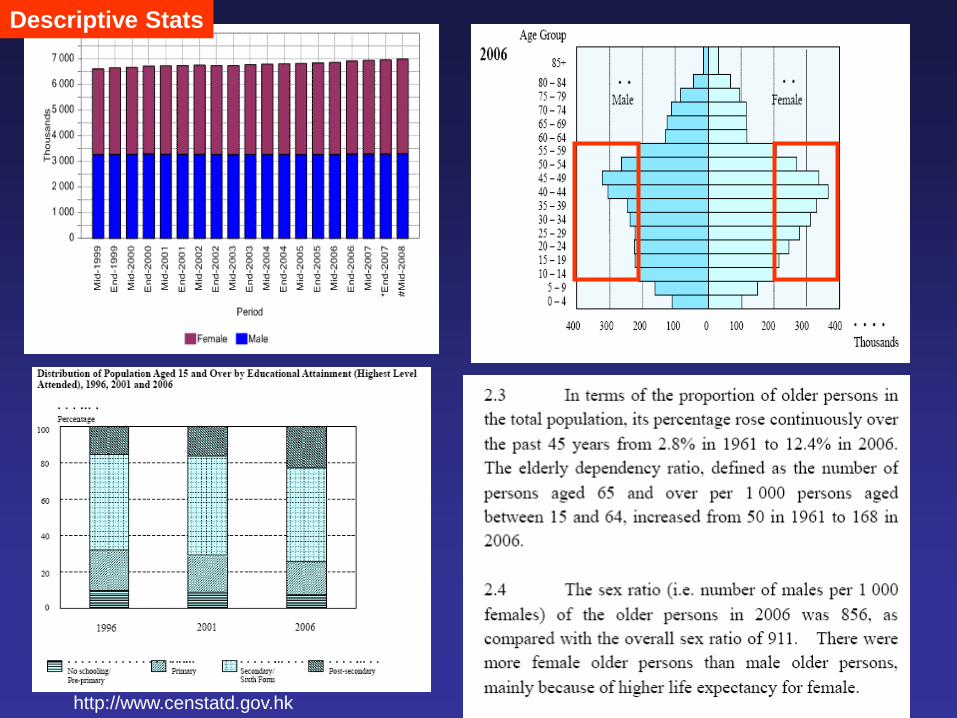
http://www.censtatd.gov.hk
Descriptive Stats
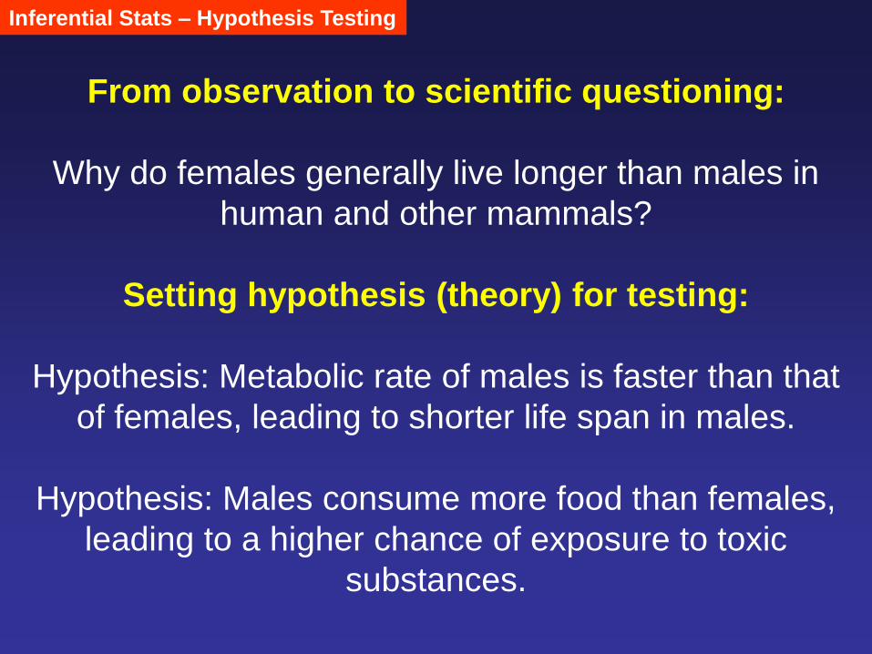
From observation to scientific questioning:
Why do females generally live longer than males in
human and other mammals?
Setting hypothesis (theory) for testing:
Hypothesis: Metabolic rate of males is faster than that
of females, leading to shorter life span in males.
Hypothesis: Males consume more food than females,
leading to a higher chance of exposure to toxic
substances.
Inferential Stats – Hypothesis Testing
A Hypothesis
• A statement relating to an observation that
may be true but for which a proof (or
disproof) has not been found.
• The results of a well-designed experiment
may lead to the proof or disproof of a
hypothesis (i.e. accept or reject of the
corresponding null hypothesis).
Inferential Stats
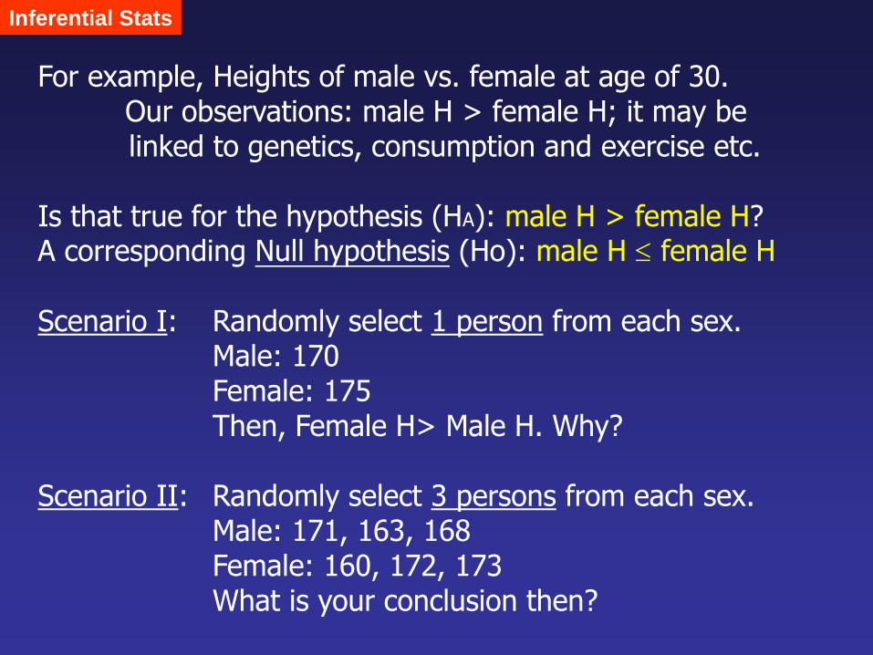
For example, Heights of male vs. female at age of 30. Our observations: male H > female H; it may be linked to genetics, consumption and exercise etc. Is that true for the hypothesis (HA): male H > female H? A corresponding Null hypothesis (Ho): male H female H Scenario I: Randomly select 1 person from each sex. Male: 170 Female: 175 Then, Female H> Male H. Why? Scenario II: Randomly select 3 persons from each sex. Male: 171, 163, 168 Female: 160, 172, 173 What is your conclusion then?
Inferential Stats
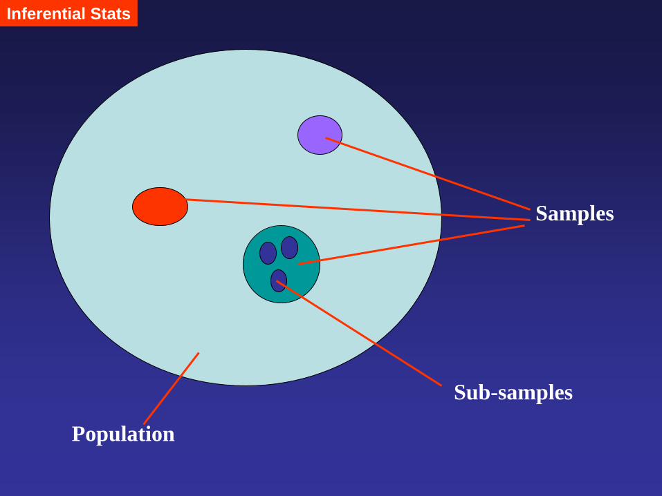
Population
Samples
Sub-samples
Inferential Stats
0.00
0.01
0.02
0.03
0.04
0.05
0.06
0.07
0.08
0.09
0.10
140 150 160 170 180 190
Height (cm)
Pro
bab
ility
de
nsi
ty
Inferential Stats
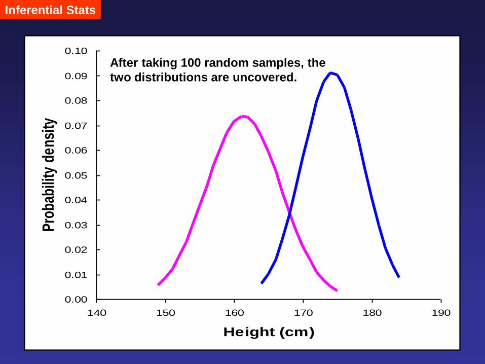
After taking 100 random samples, the
two distributions are uncovered.
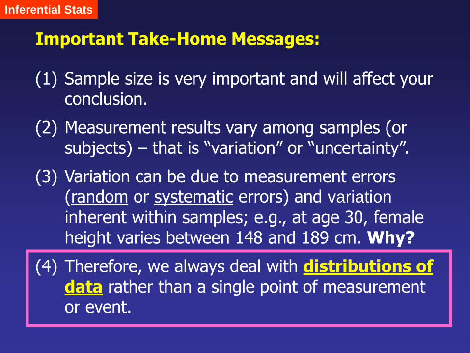
Important Take-Home Messages:
(1) Sample size is very important and will affect your conclusion.
(2) Measurement results vary among samples (or subjects) – that is “variation” or “uncertainty”.
(3) Variation can be due to measurement errors (random or systematic errors) and variation
inherent within samples; e.g., at age 30, female height varies between 148 and 189 cm. Why?
(4) Therefore, we always deal with distributions of data rather than a single point of measurement or event.
Inferential Stats
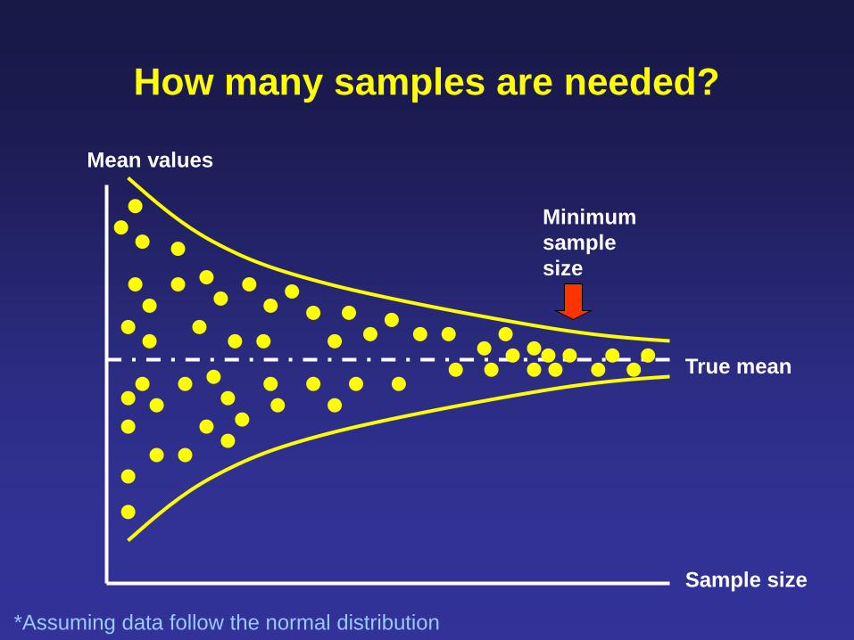
How many samples are needed?
Mean values
Sample size
True mean
Minimum
sample
size
*Assuming data follow the normal distribution
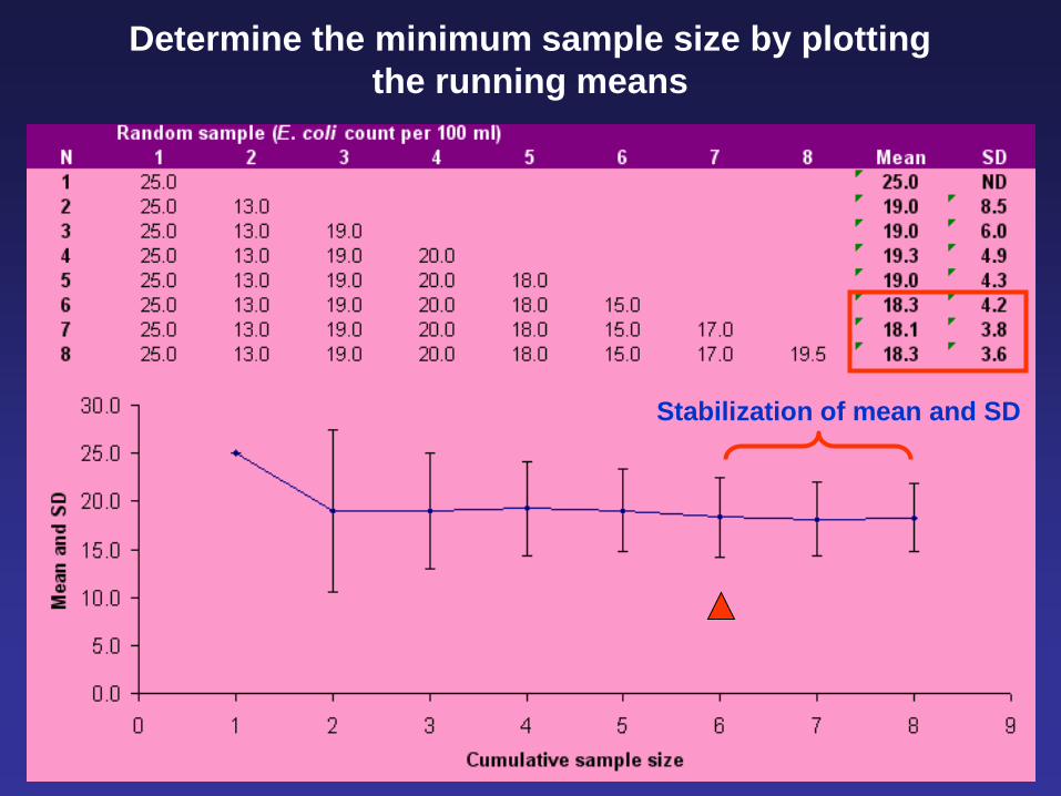
Determine the minimum sample size by plotting
the running means
Stabilization of mean and SD
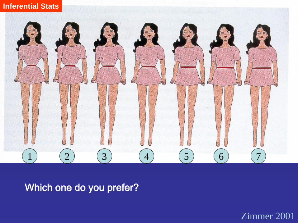
Zimmer 2001
1 2 3 4 5 6 7
Which one do you prefer?
Inferential Stats
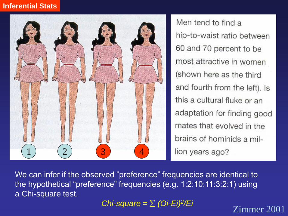
1 2 3 4
Zimmer 2001
We can infer if the observed “preference” frequencies are identical to
the hypothetical “preference” frequencies (e.g. 1:2:10:11:3:2:1) using
a Chi-square test.
Chi-square = (Oi-Ei)2/Ei
Inferential Stats
Inferential Stats – Hypothesis Testing
Ho 1: The water sample A is cleaner than the water
sample B in terms of E. coli count.
Ho 2: Water quality in Site A is better than Site B in
terms of E. coli count during the swimming
season.
Ho 3: Water quality in Site A is better than Site B in
terms of E. coli count at all times.
How can we test the following hypotheses?
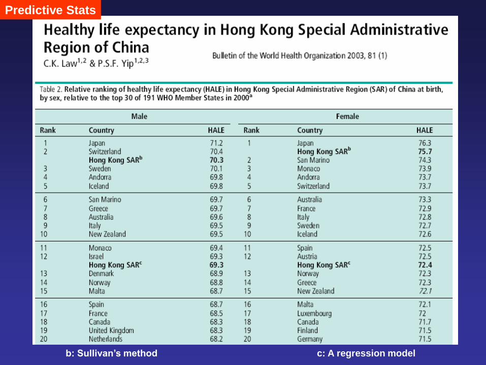
b: Sullivan’s method c: A regression model
Predictive Stats
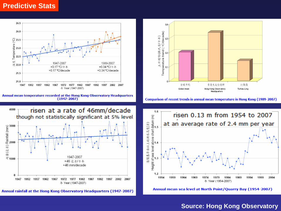
Predictive Stats
Source: Hong Kong Observatory
Basic Descriptive Statistics
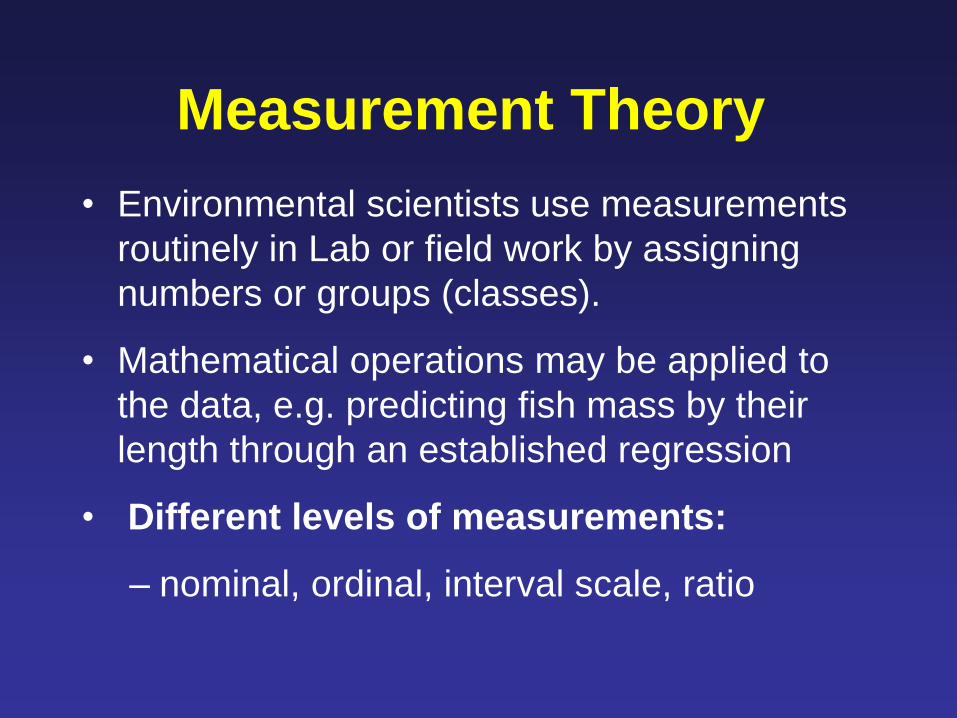
Measurement Theory
• Environmental scientists use measurements
routinely in Lab or field work by assigning
numbers or groups (classes).
• Mathematical operations may be applied to
the data, e.g. predicting fish mass by their
length through an established regression
• Different levels of measurements:
– nominal, ordinal, interval scale, ratio
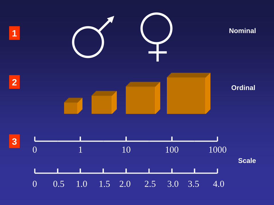
1
2
3 0 1 10 100 1000
0 0.5 1.0 1.5 2.0 2.5 3.0 3.5 4.0
Nominal
Ordinal
Scale
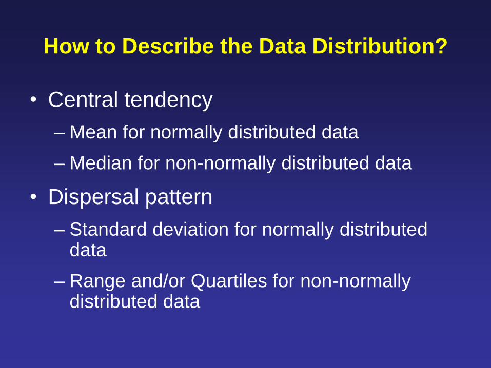
How to Describe the Data Distribution?
• Central tendency
– Mean for normally distributed data
– Median for non-normally distributed data
• Dispersal pattern
– Standard deviation for normally distributed data
– Range and/or Quartiles for non-normally distributed data

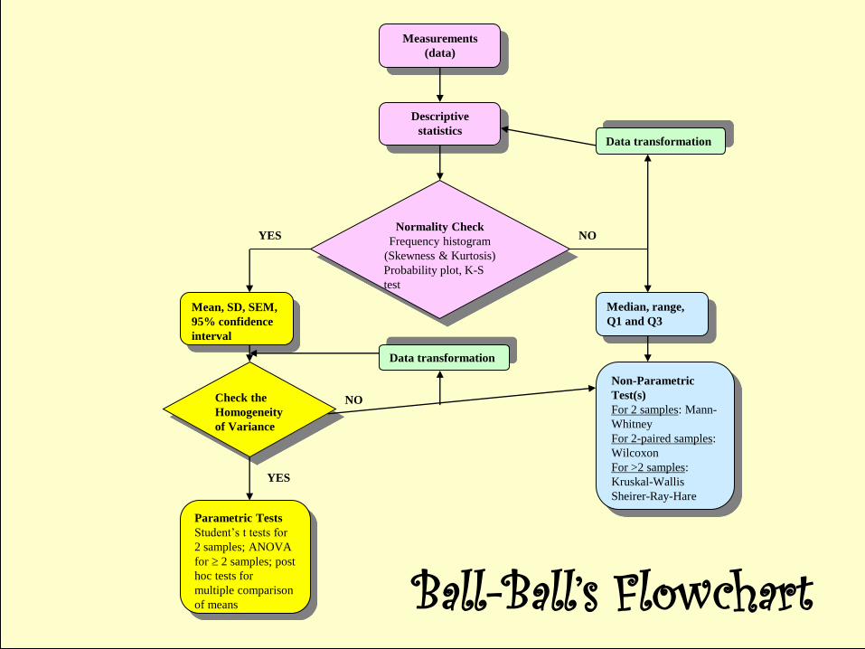
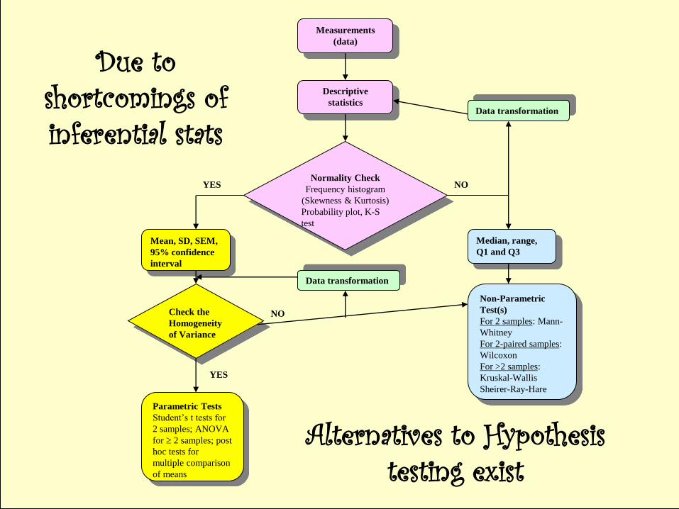
Normality Check
Frequency histogram
(Skewness & Kurtosis)
Probability plot, K-S
test
Descriptive
statistics
Measurements
(data)
Mean, SD, SEM,
95% confidence
interval
YES
Check the
Homogeneity
of Variance
Data transformation
NO
Data transformation
NO
Median, range,
Q1 and Q3
Non-Parametric
Test(s)
For 2 samples: Mann-
Whitney
For 2-paired samples:
Wilcoxon
For >2 samples:
Kruskal-Wallis
Sheirer-Ray-Hare
Parametric Tests
Student’s t tests for
2 samples; ANOVA
for 2 samples; post
hoc tests for
multiple comparison
of means
YES
Ball-Ball’s Flowchart
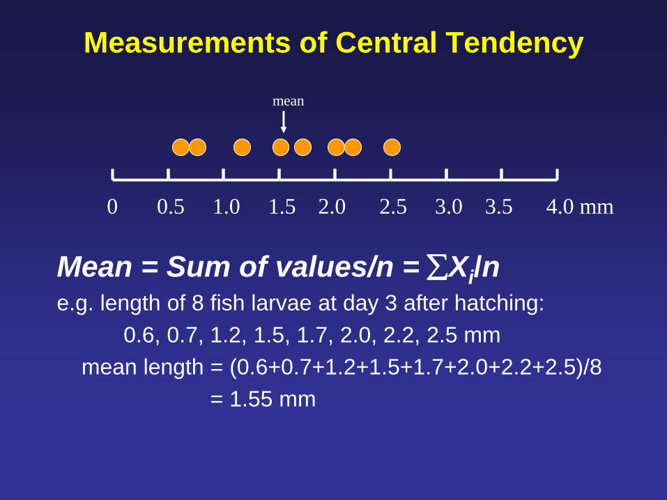
Measurements of Central Tendency
Mean = Sum of values/n = Xi/n e.g. length of 8 fish larvae at day 3 after hatching:
0.6, 0.7, 1.2, 1.5, 1.7, 2.0, 2.2, 2.5 mm
mean length = (0.6+0.7+1.2+1.5+1.7+2.0+2.2+2.5)/8
= 1.55 mm
0 0.5 1.0 1.5 2.0 2.5 3.0 3.5 4.0 mm
mean
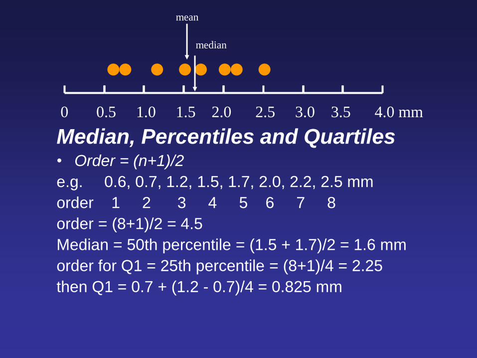
Median, Percentiles and Quartiles • Order = (n+1)/2
e.g. 0.6, 0.7, 1.2, 1.5, 1.7, 2.0, 2.2, 2.5 mm
order 1 2 3 4 5 6 7 8
order = (8+1)/2 = 4.5
Median = 50th percentile = (1.5 + 1.7)/2 = 1.6 mm
order for Q1 = 25th percentile = (8+1)/4 = 2.25
then Q1 = 0.7 + (1.2 - 0.7)/4 = 0.825 mm
0 0.5 1.0 1.5 2.0 2.5 3.0 3.5 4.0 mm
mean
median
0 0.5 1.0 1.5 2.0 2.5 3.0 3.5 4.0 mm
mean
median
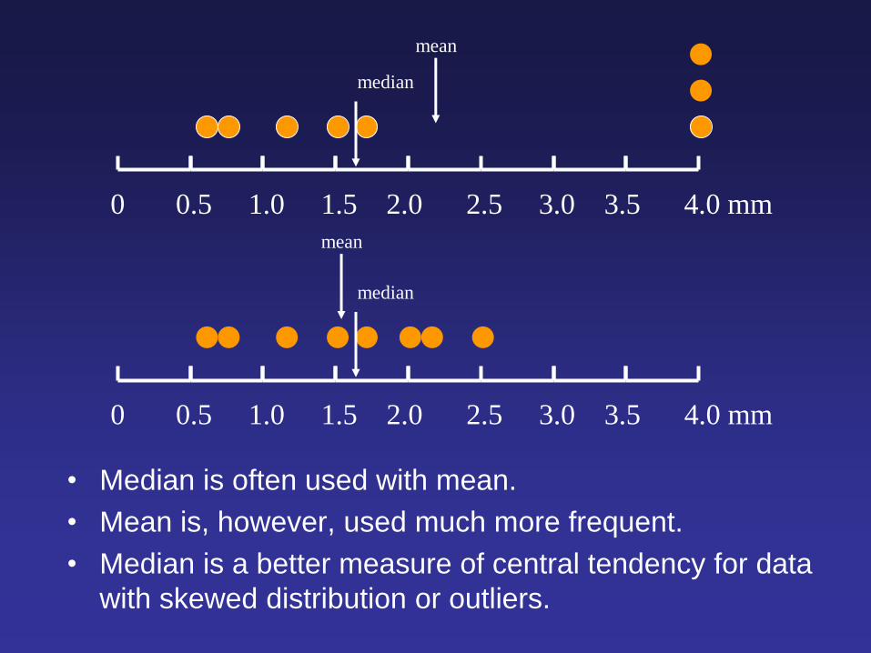
• Median is often used with mean.
• Mean is, however, used much more frequent.
• Median is a better measure of central tendency for data
with skewed distribution or outliers.
0 0.5 1.0 1.5 2.0 2.5 3.0 3.5 4.0 mm
mean
median
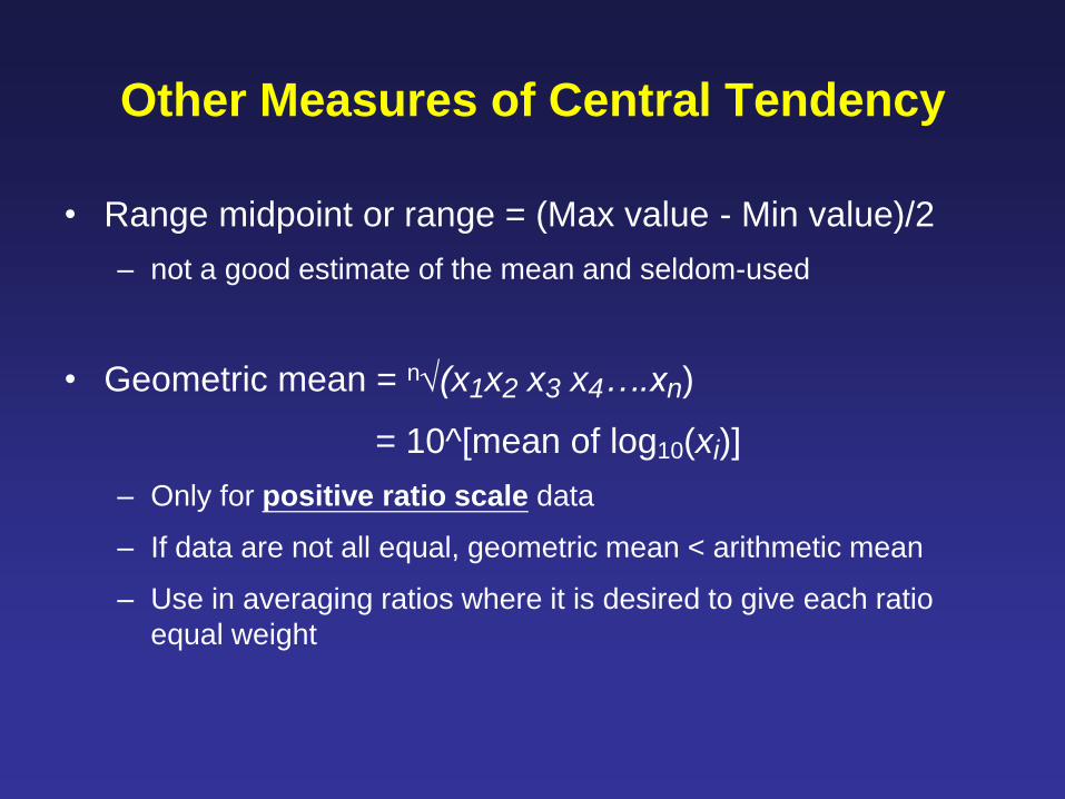
Other Measures of Central Tendency
• Range midpoint or range = (Max value - Min value)/2
– not a good estimate of the mean and seldom-used
• Geometric mean = n(x1x2 x3 x4….xn)
= 10^[mean of log10(xi)]
– Only for positive ratio scale data
– If data are not all equal, geometric mean < arithmetic mean
– Use in averaging ratios where it is desired to give each ratio
equal weight
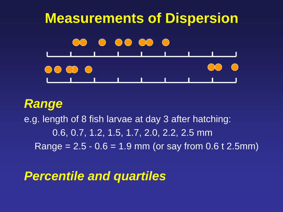
Measurements of Dispersion
Range e.g. length of 8 fish larvae at day 3 after hatching:
0.6, 0.7, 1.2, 1.5, 1.7, 2.0, 2.2, 2.5 mm
Range = 2.5 - 0.6 = 1.9 mm (or say from 0.6 t 2.5mm)
Percentile and quartiles
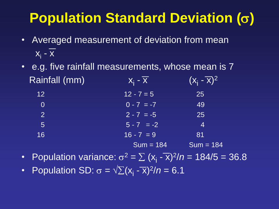
Population Standard Deviation ()
• Averaged measurement of deviation from mean
xi - x
• e.g. five rainfall measurements, whose mean is 7
Rainfall (mm) xi - x (xi - x)2
12 12 - 7 = 5 25
0 0 - 7 = -7 49
2 2 - 7 = -5 25
5 5 - 7 = -2 4
16 16 - 7 = 9 81
Sum = 184 Sum = 184
• Population variance: 2 = (xi - x)2/n = 184/5 = 36.8
• Population SD: = (xi - x)2/n = 6.1
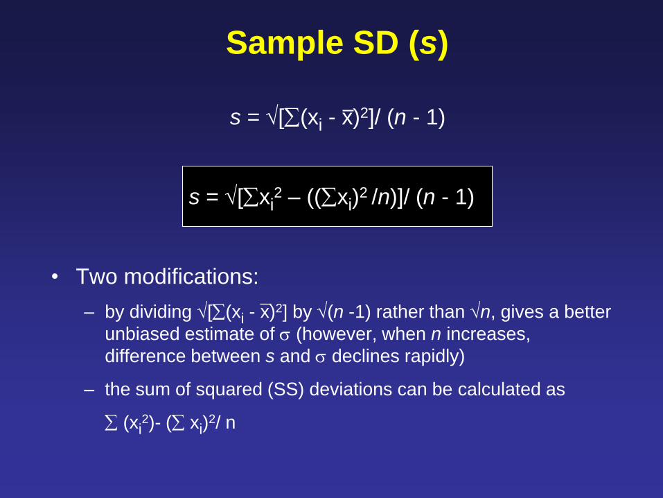
Sample SD (s)
s = [(xi - x)2]/ (n - 1)
s = [xi2 – ((xi)
2 /n)]/ (n - 1)
• Two modifications:
– by dividing [(xi - x)2] by (n -1) rather than n, gives a better
unbiased estimate of (however, when n increases,
difference between s and declines rapidly)
– the sum of squared (SS) deviations can be calculated as
(xi2)- ( xi)
2/ n
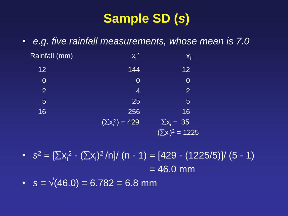
Sample SD (s)
• e.g. five rainfall measurements, whose mean is 7.0
Rainfall (mm) xi2 xi
12 144 12
0 0 0
2 4 2
5 25 5
16 256 16
(xi2) = 429 xi = 35
(xi)2 = 1225
• s2 = [xi2 - (xi)
2 /n]/ (n - 1) = [429 - (1225/5)]/ (5 - 1)
= 46.0 mm
• s = (46.0) = 6.782 = 6.8 mm
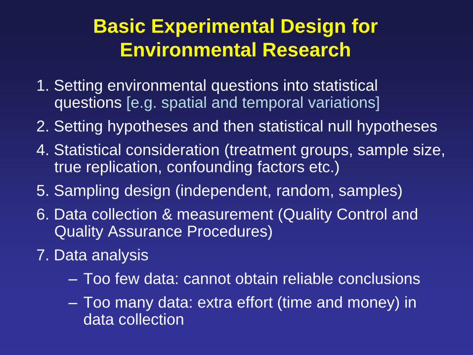
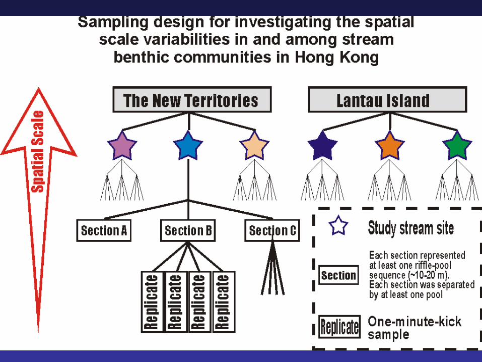
Basic Experimental Design for
Environmental Research
1. Setting environmental questions into statistical questions [e.g. spatial and temporal variations]
2. Setting hypotheses and then statistical null hypotheses
4. Statistical consideration (treatment groups, sample size, true replication, confounding factors etc.)
5. Sampling design (independent, random, samples)
6. Data collection & measurement (Quality Control and Quality Assurance Procedures)
7. Data analysis
– Too few data: cannot obtain reliable conclusions
– Too many data: extra effort (time and money) in data collection
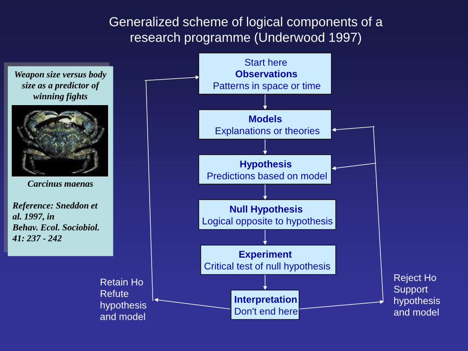
Generalized scheme of logical components of a
research programme (Underwood 1997)
Weapon size versus body
size as a predictor of
winning fights
Carcinus maenas
Reference: Sneddon et
al. 1997, in
Behav. Ecol. Sociobiol.
41: 237 - 242
Reject Ho
Support
hypothesis
and model
Retain Ho
Refute
hypothesis
and model
Interpretation
Don't end here
Experiment
Critical test of null hypothesis
Null Hypothesis
Logical opposite to hypothesis
Hypothesis
Predictions based on model
Models
Explanations or theories
Start here
Observations
Patterns in space or time
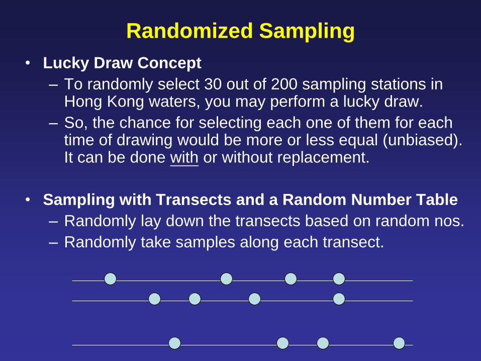
Randomized Sampling
• Lucky Draw Concept
– To randomly select 30 out of 200 sampling stations in Hong Kong waters, you may perform a lucky draw.
– So, the chance for selecting each one of them for each time of drawing would be more or less equal (unbiased). It can be done with or without replacement.
• Sampling with Transects and a Random Number Table
– Randomly lay down the transects based on random nos.
– Randomly take samples along each transect.
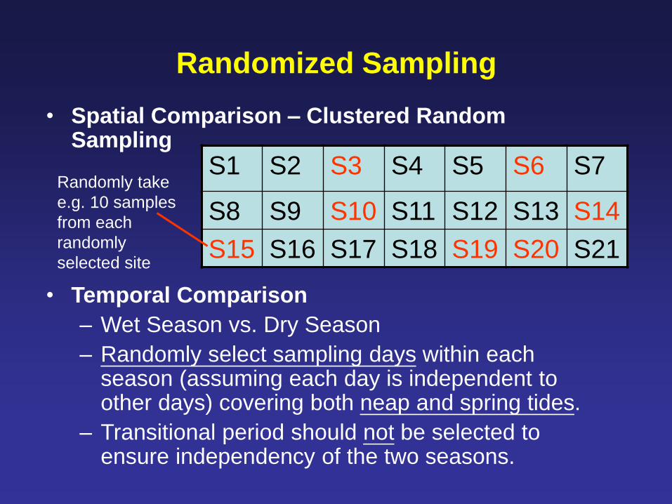
Randomized Sampling
• Spatial Comparison – Clustered Random Sampling
S1 S2 S3 S4 S5 S6 S7
S8 S9 S10 S11 S12 S13 S14
S15 S16 S17 S18 S19 S20 S21
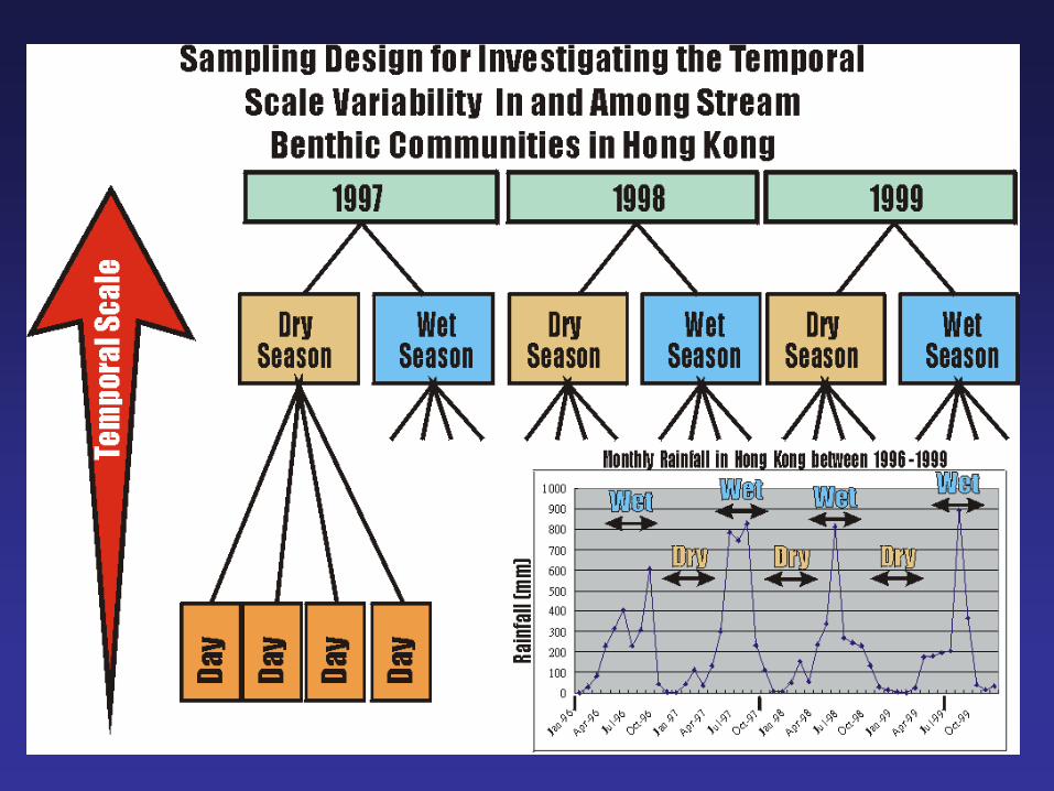
• Temporal Comparison
– Wet Season vs. Dry Season
– Randomly select sampling days within each season (assuming each day is independent to other days) covering both neap and spring tides.
– Transitional period should not be selected to ensure independency of the two seasons.
Randomly take
e.g. 10 samples
from each
randomly
selected site
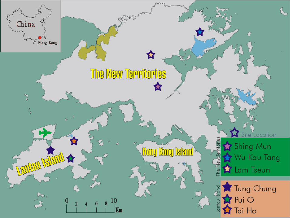
Study Sites (HK map)
Spatial
Temporal
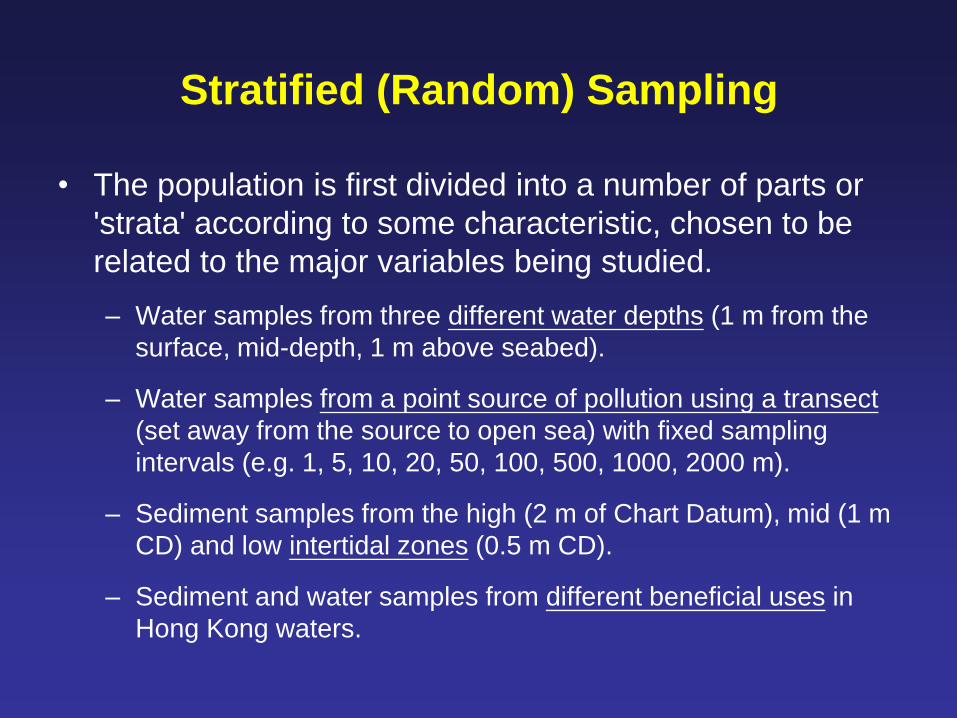
Stratified (Random) Sampling
• The population is first divided into a number of parts or
'strata' according to some characteristic, chosen to be
related to the major variables being studied.
– Water samples from three different water depths (1 m from the
surface, mid-depth, 1 m above seabed).
– Water samples from a point source of pollution using a transect
(set away from the source to open sea) with fixed sampling
intervals (e.g. 1, 5, 10, 20, 50, 100, 500, 1000, 2000 m).
– Sediment samples from the high (2 m of Chart Datum), mid (1 m
CD) and low intertidal zones (0.5 m CD).
– Sediment and water samples from different beneficial uses in
Hong Kong waters.
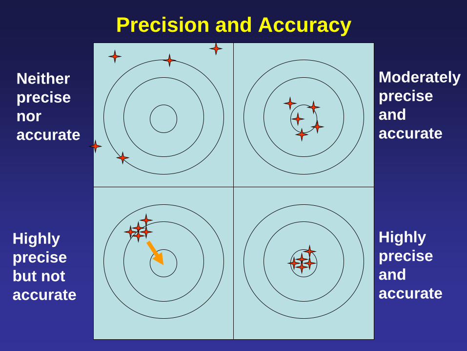
Precision and Accuracy
Neither
precise
nor
accurate
Highly
precise
but not
accurate
Moderately
precise
and
accurate
Highly
precise
and
accurate
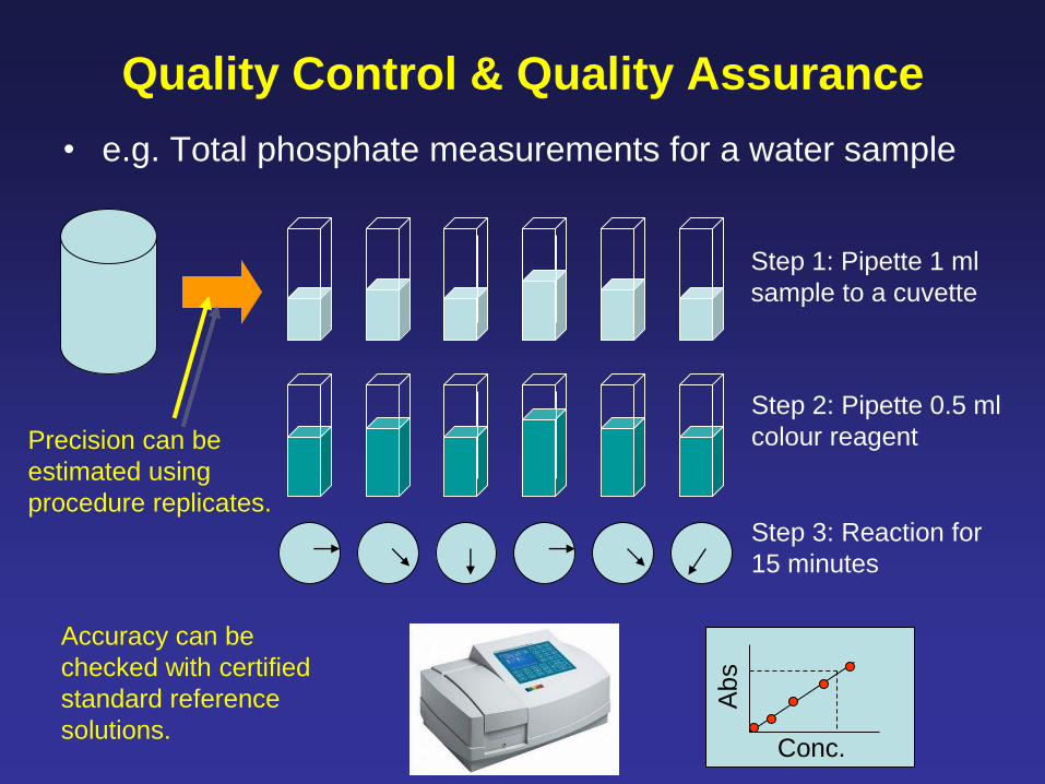
Quality Control & Quality Assurance
• e.g. Total phosphate measurements for a water sample
Step 1: Pipette 1 ml
sample to a cuvette
Step 2: Pipette 0.5 ml
colour reagent
Step 3: Reaction for
15 minutes
Conc. A
bs
Accuracy can be
checked with certified
standard reference
solutions.
Precision can be
estimated using
procedure replicates.
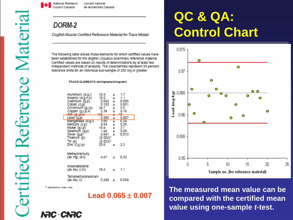
Lead 0.065 0.007
QC & QA:
Control Chart
The measured mean value can be
compared with the certified mean
value using one-sample t-test.
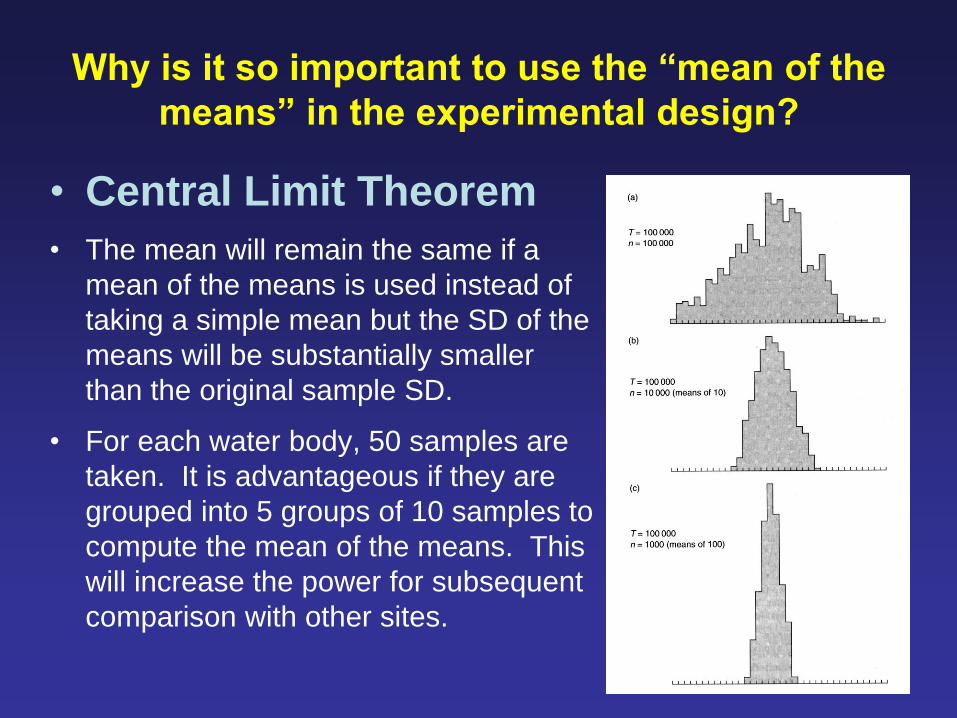
Why is it so important to use the “mean of the
means” in the experimental design?
• Central Limit Theorem
• The mean will remain the same if a
mean of the means is used instead of
taking a simple mean but the SD of the
means will be substantially smaller
than the original sample SD.
• For each water body, 50 samples are
taken. It is advantageous if they are
grouped into 5 groups of 10 samples to
compute the mean of the means. This
will increase the power for subsequent
comparison with other sites.
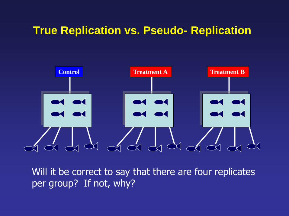
True Replication vs. Pseudo- Replication
Treatment B Control Treatment A
Will it be correct to say that there are four replicates per group? If not, why?
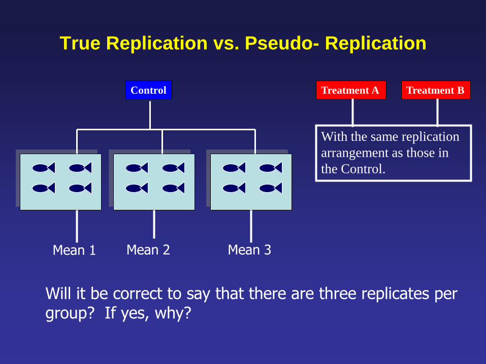
True Replication vs. Pseudo- Replication
Treatment B Control Treatment A
Will it be correct to say that there are three replicates per group? If yes, why?
Mean 1 Mean 2 Mean 3
With the same replication
arrangement as those in
the Control.
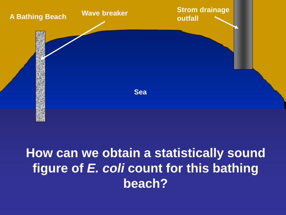
How can we obtain a statistically sound
figure of E. coli count for this bathing
beach?
Strom drainage
outfall A Bathing Beach Wave breaker
Sea
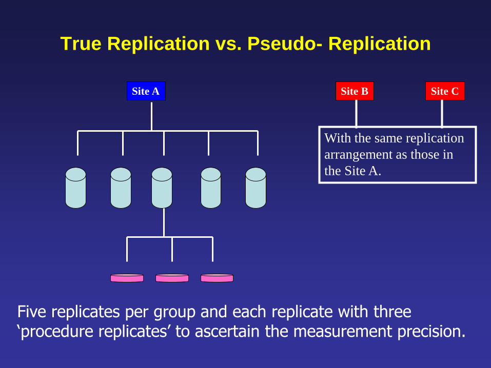
True Replication vs. Pseudo- Replication
Site C Site A Site B
Five replicates per group and each replicate with three ‘procedure replicates’ to ascertain the measurement precision.
With the same replication
arrangement as those in
the Site A.
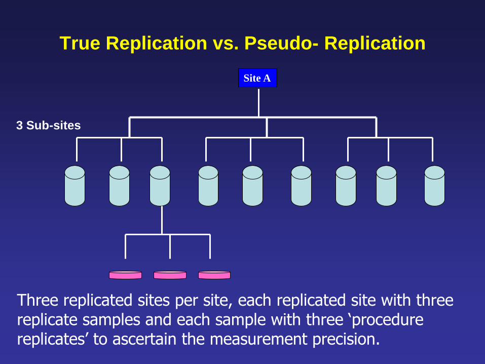
True Replication vs. Pseudo- Replication
Site A
Three replicated sites per site, each replicated site with three replicate samples and each sample with three ‘procedure replicates’ to ascertain the measurement precision.
3 Sub-sites
Inferential Statistics
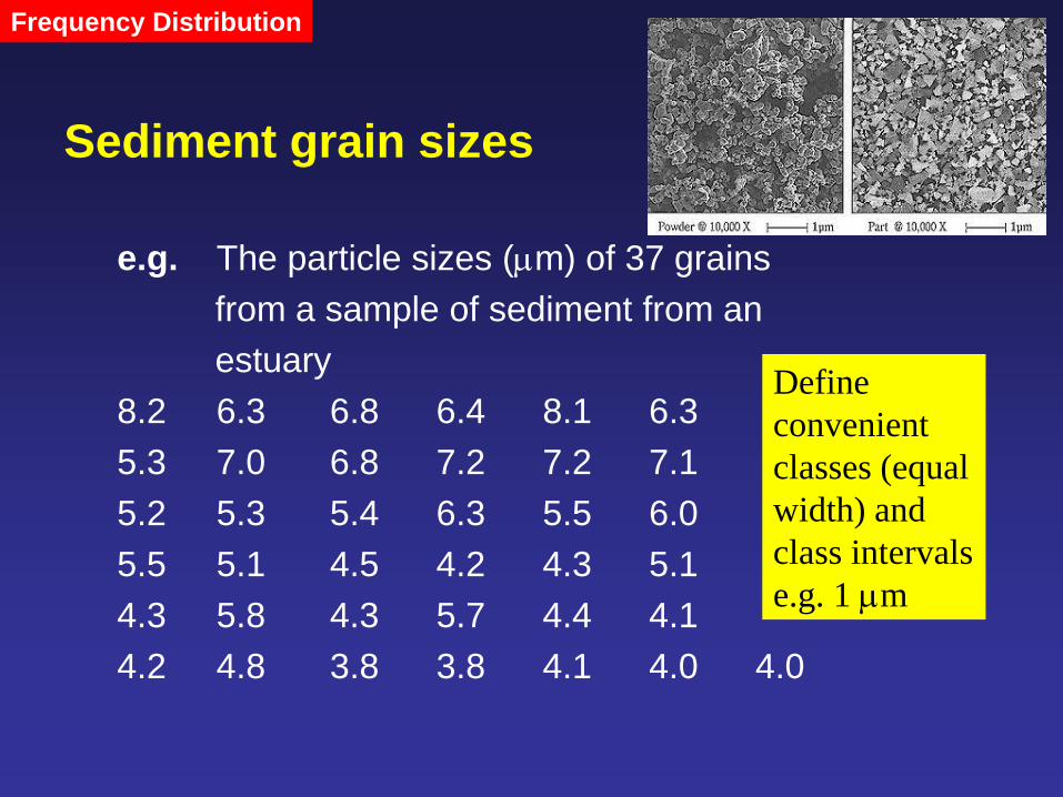
e.g. The particle sizes (m) of 37 grains
from a sample of sediment from an
estuary
8.2 6.3 6.8 6.4 8.1 6.3
5.3 7.0 6.8 7.2 7.2 7.1
5.2 5.3 5.4 6.3 5.5 6.0
5.5 5.1 4.5 4.2 4.3 5.1
4.3 5.8 4.3 5.7 4.4 4.1
4.2 4.8 3.8 3.8 4.1 4.0 4.0
Define
convenient
classes (equal
width) and
class intervals
e.g. 1 m
Frequency Distribution
Sediment grain sizes
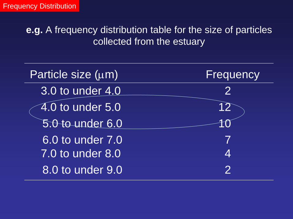
e.g. A frequency distribution table for the size of particles
collected from the estuary
Particle size (m) Frequency
3.0 to under 4.0 2
4.0 to under 5.0 12
5.0 to under 6.0 10
6.0 to under 7.0 7
7.0 to under 8.0 4
8.0 to under 9.0 2
Frequency Distribution
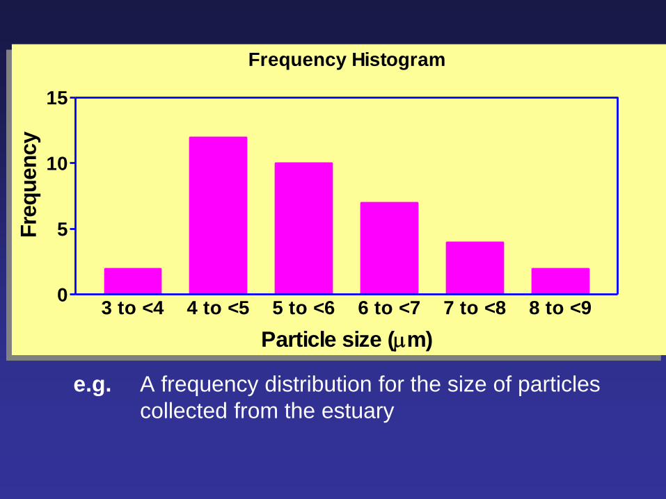
e.g. A frequency distribution for the size of particles
collected from the estuary
Frequency Histogram
3 to <4 4 to <5 5 to <6 6 to <7 7 to <8 8 to <90
5
10
15
Particle size (m)
Fre
qu
en
cy
>149-153>153-157>157-161>161-165>165-169>169-173>173-177>177-181>181-1850
2
4
6
8
10
12
14
Height (cm)
Fre
qu
en
cy
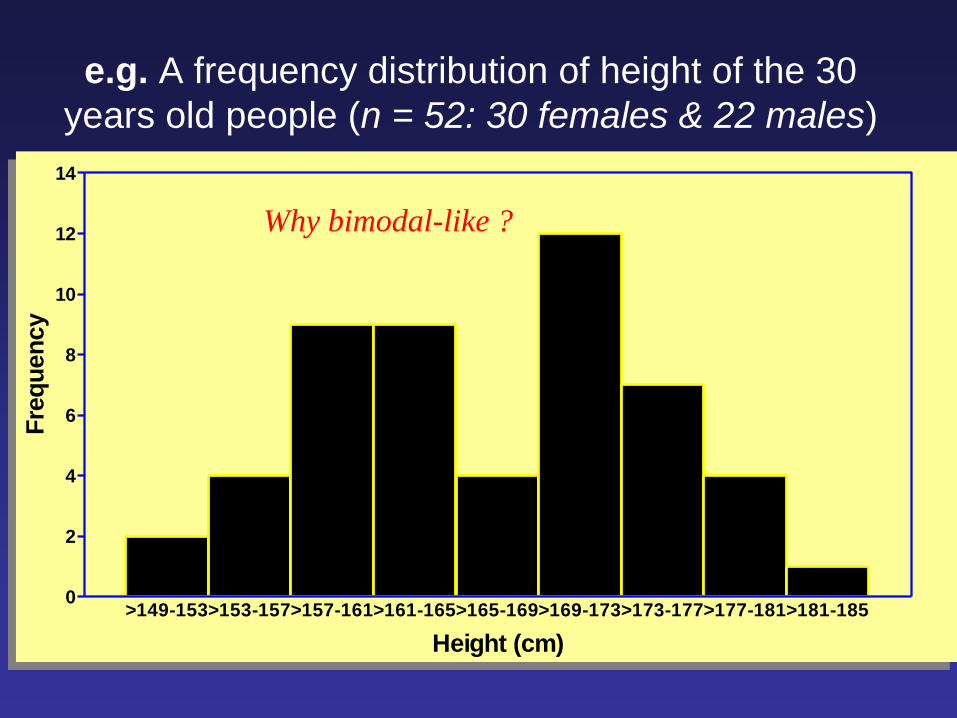
e.g. A frequency distribution of height of the 30
years old people (n = 52: 30 females & 22 males)
Why bimodal-like ?
0.00
0.01
0.02
0.03
0.04
0.05
0.06
0.07
0.08
0.09
0.10
140 150 160 170 180 190
Height (cm)
Pro
bab
ilit
y d
en
sit
y
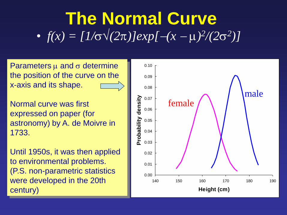
Parameters and determine
the position of the curve on the
x-axis and its shape.
Normal curve was first
expressed on paper (for
astronomy) by A. de Moivre in
1733.
Until 1950s, it was then applied
to environmental problems.
(P.S. non-parametric statistics
were developed in the 20th
century)
female male
The Normal Curve • f(x) = [1/(2)]exp[(x )2/(22)]
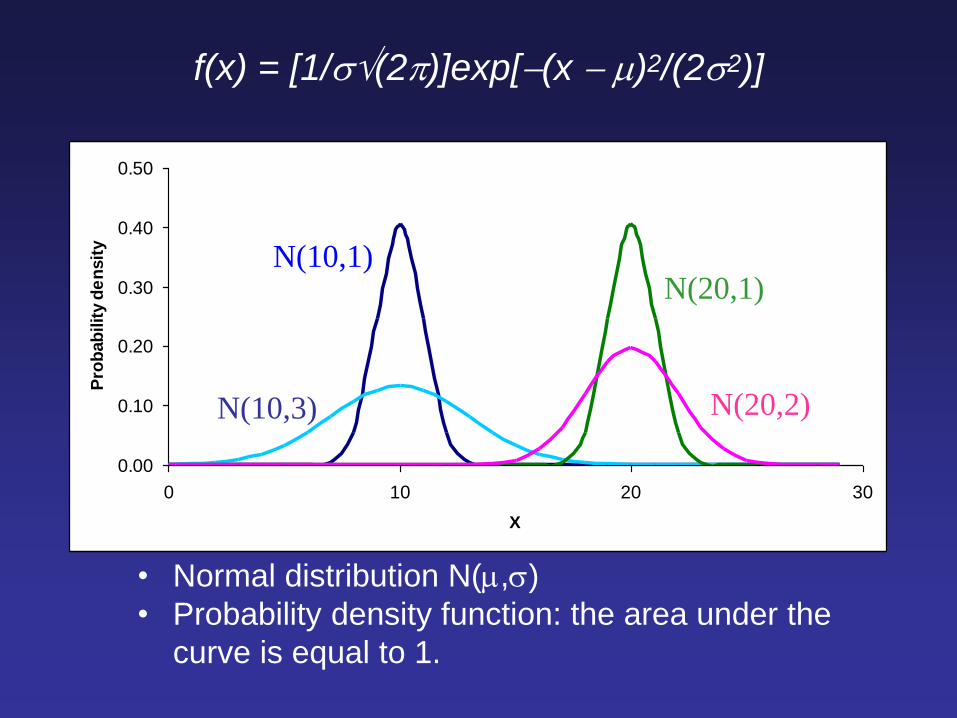
f(x) = [1/(2)]exp[(x )2/(22)]
0.00
0.10
0.20
0.30
0.40
0.50
0 10 20 30
X
Pro
bab
ilit
y d
en
sit
y
N(20,2)
N(20,1) N(10,1)
N(10,3)
• Normal distribution N(,)
• Probability density function: the area under the
curve is equal to 1.
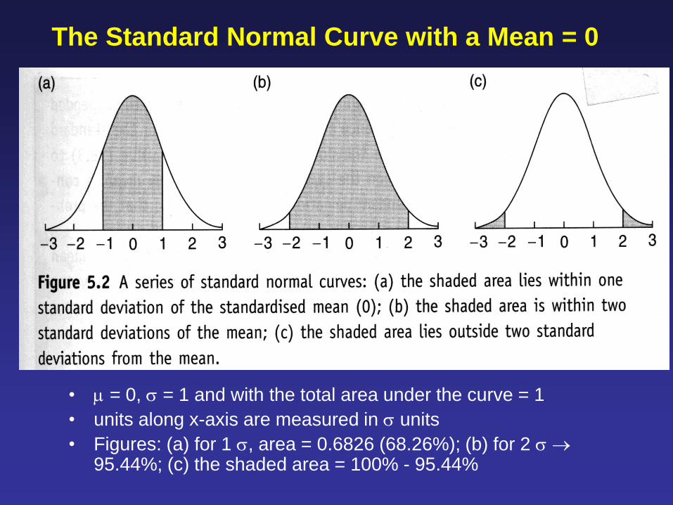
• = 0, = 1 and with the total area under the curve = 1
• units along x-axis are measured in units
• Figures: (a) for 1 , area = 0.6826 (68.26%); (b) for 2 95.44%; (c) the shaded area = 100% - 95.44%
The Standard Normal Curve with a Mean = 0
(Pentecost 1999)
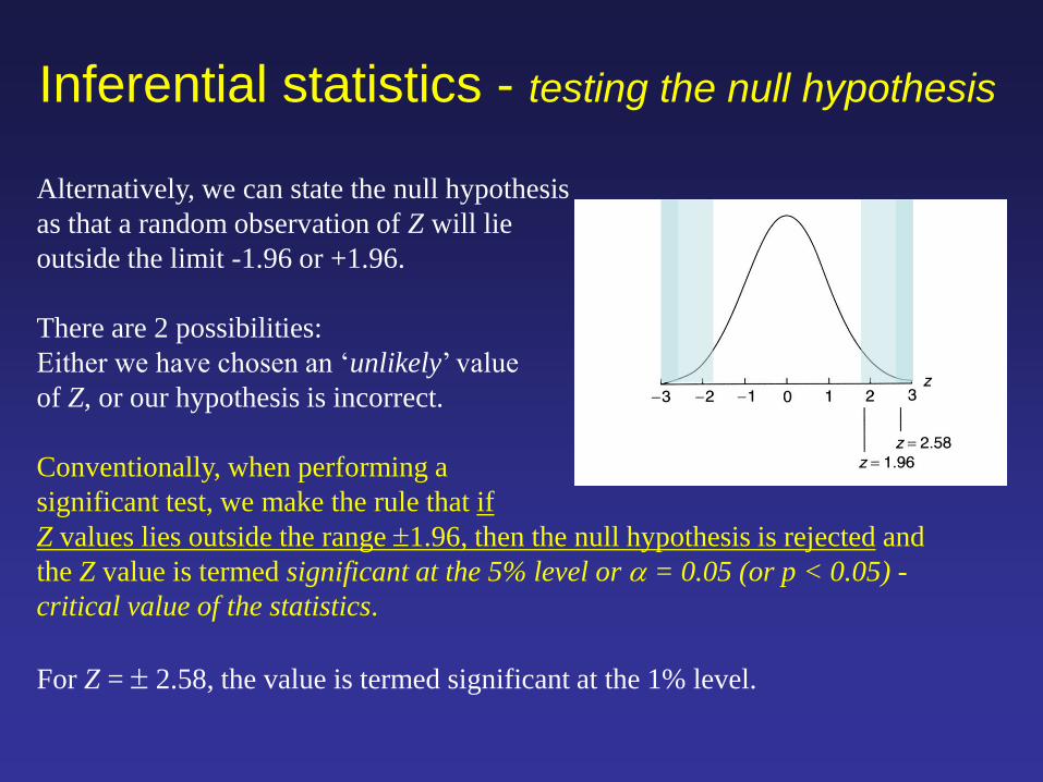
Alternatively, we can state the null hypothesis
as that a random observation of Z will lie
outside the limit -1.96 or +1.96.
There are 2 possibilities:
Either we have chosen an ‘unlikely’ value
of Z, or our hypothesis is incorrect.
Conventionally, when performing a
significant test, we make the rule that if
Z values lies outside the range 1.96, then the null hypothesis is rejected and
the Z value is termed significant at the 5% level or = 0.05 (or p < 0.05) -
critical value of the statistics.
For Z = 2.58, the value is termed significant at the 1% level.
Inferential statistics - testing the null hypothesis
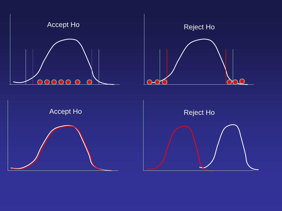
Accept Ho Reject Ho
Accept Ho Reject Ho

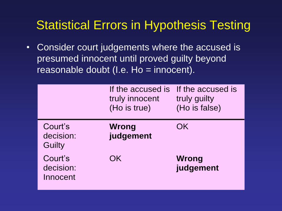
Statistical Errors in Hypothesis Testing
• Consider court judgements where the accused is
presumed innocent until proved guilty beyond
reasonable doubt (I.e. Ho = innocent).
If the accused is truly innocent (Ho is true)
If the accused is truly guilty (Ho is false)
Court’s decision: Guilty
Wrong judgement
OK
Court’s decision: Innocent
OK Wrong judgement
Statistical Errors in Hypothesis Testing
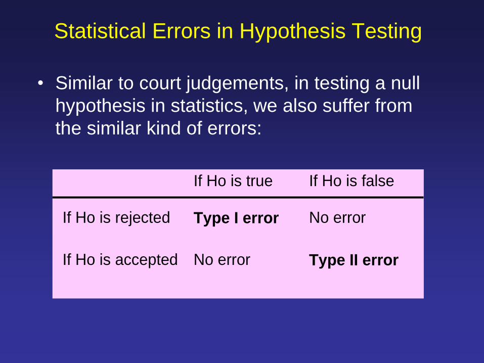
• Similar to court judgements, in testing a null
hypothesis in statistics, we also suffer from
the similar kind of errors:
If Ho is true If Ho is false
If Ho is rejected Type I error No error
If Ho is accepted No error Type II error
Statistical Errors in Hypothesis Testing
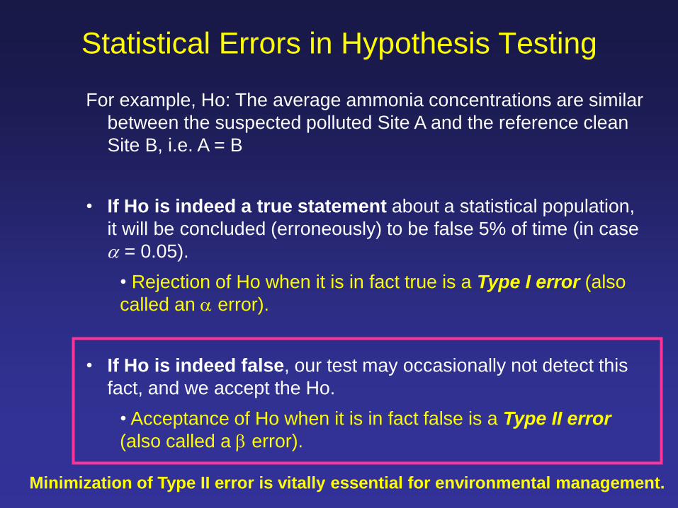
For example, Ho: The average ammonia concentrations are similar
between the suspected polluted Site A and the reference clean
Site B, i.e. A = B
• If Ho is indeed a true statement about a statistical population,
it will be concluded (erroneously) to be false 5% of time (in case
= 0.05).
• Rejection of Ho when it is in fact true is a Type I error (also
called an error).
• If Ho is indeed false, our test may occasionally not detect this
fact, and we accept the Ho.
• Acceptance of Ho when it is in fact false is a Type II error
(also called a error).
Minimization of Type II error is vitally essential for environmental management.
Power of a Statistical Test
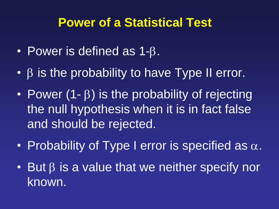
• Power is defined as 1-.
• is the probability to have Type II error.
• Power (1- ) is the probability of rejecting
the null hypothesis when it is in fact false
and should be rejected.
• Probability of Type I error is specified as .
• But is a value that we neither specify nor
known.
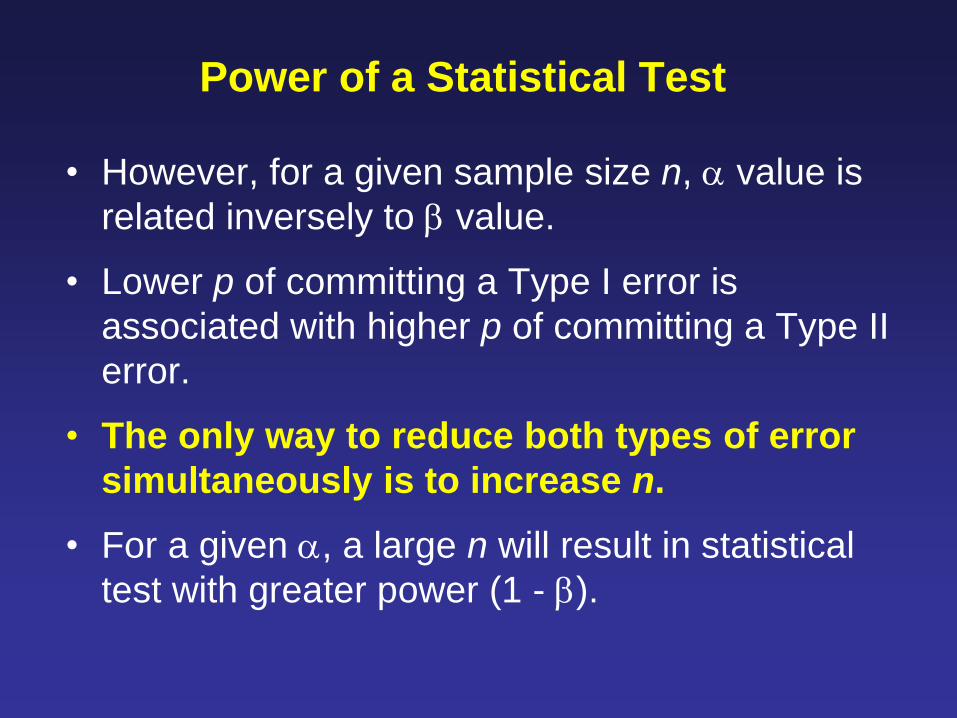
• However, for a given sample size n, value is
related inversely to value.
• Lower p of committing a Type I error is
associated with higher p of committing a Type II
error.
• The only way to reduce both types of error
simultaneously is to increase n.
• For a given , a large n will result in statistical
test with greater power (1 - ).
Power of a Statistical Test
What is next?
1. Group Discussion on the Experimental
Design for a Case Study
2. Introduction to Two Classes of Basic
Statistical Techniques:
(1) correlation based methods and
(2) group comparison methods
3. Power Analysis
Normality Check
Frequency histogram
(Skewness & Kurtosis)
Probability plot, K-S
test
Descriptive
statistics
Measurements
(data)
Mean, SD, SEM,
95% confidence
interval
YES
Check the
Homogeneity
of Variance
Data transformation
NO
Data transformation
NO
Median, range,
Q1 and Q3
Non-Parametric
Test(s)
For 2 samples: Mann-
Whitney
For 2-paired samples:
Wilcoxon
For >2 samples:
Kruskal-Wallis
Sheirer-Ray-Hare
Parametric Tests
Student’s t tests for
2 samples; ANOVA
for 2 samples; post
hoc tests for
multiple comparison
of means
YES
Ball-Ball’s Flowchart
A. Comparing Two Samples
Independent Samples t test
B. Comparing More than 2 Samples
Analysis of Variance (ANOVA)
Power Analysis with G*Power

G*Power 3 – Free Software
http://www.psycho.uni-duesseldorf.de/abteilungen/aap/gpower3/

Photo source: http://www-groups.dcs.st-and.ac.uk/~history/PictDisplay/Gosset.html
Mr. Student = Mr. William Sealey Gosset (1876 – 1937)

Normality Check
Frequency histogram
(Skewness & Kurtosis)
Probability plot, K-S
test
Descriptive
statistics
Measurements
(data)
Mean, SD, SEM,
95% confidence
interval
YES
Check the
Homogeneity
of Variance
Data transformation
NO
Data transformation
NO
Median, range,
Q1 and Q3
Non-Parametric
Test(s)
For 2 samples: Mann-
Whitney
For 2-paired samples:
Wilcoxon
For >2 samples:
Kruskal-Wallis
Sheirer-Ray-Hare
Parametric Tests
Student’s t tests for
2 samples; ANOVA
for 2 samples; post
hoc tests for
multiple comparison
of means
YES
Ball-Ball’s Flowchart
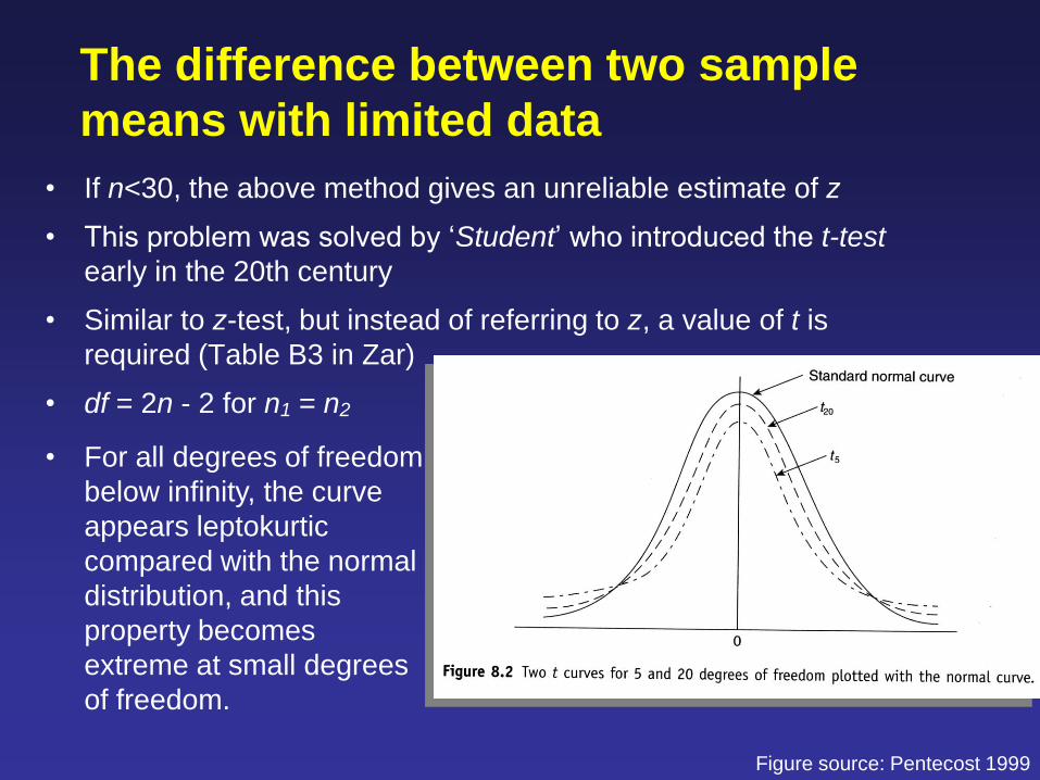
The difference between two sample
means with limited data
• If n<30, the above method gives an unreliable estimate of z
• This problem was solved by ‘Student’ who introduced the t-test
early in the 20th century
• Similar to z-test, but instead of referring to z, a value of t is
required (Table B3 in Zar)
• df = 2n - 2 for n1 = n2
• For all degrees of freedom
below infinity, the curve
appears leptokurtic
compared with the normal
distribution, and this
property becomes
extreme at small degrees
of freedom.
Figure source: Pentecost 1999
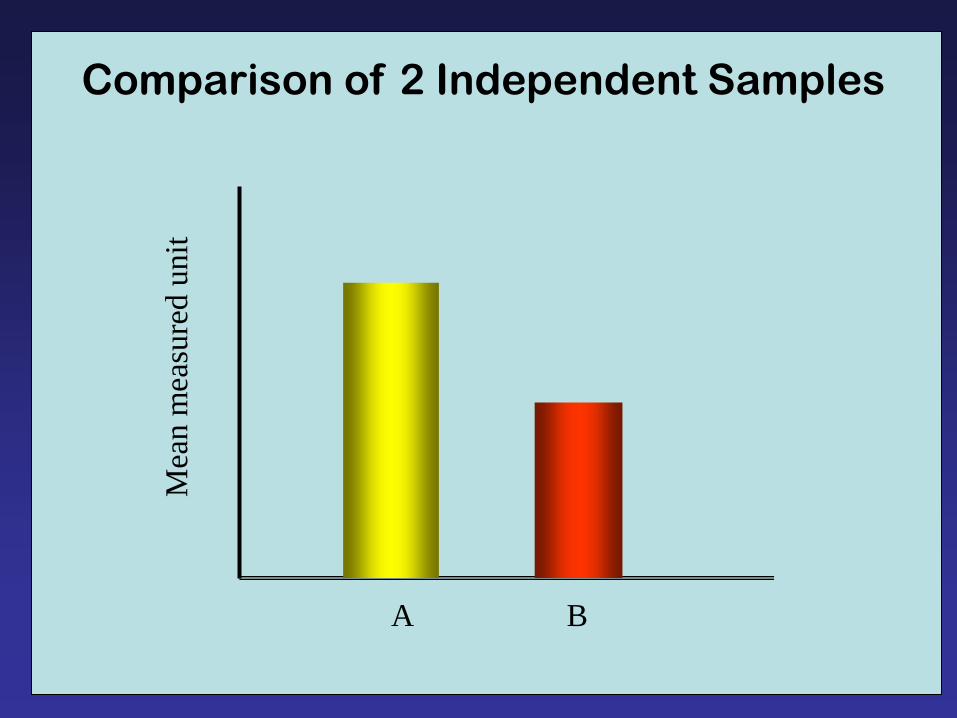
A B
Mea
n m
easu
red u
nit
Comparison of 2 Independent Samples
Error bar = 95% C.I.
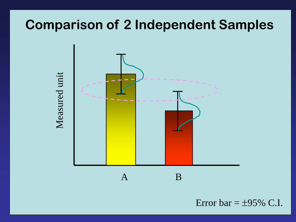
A B
Mea
sure
d u
nit
Comparison of 2 Independent Samples
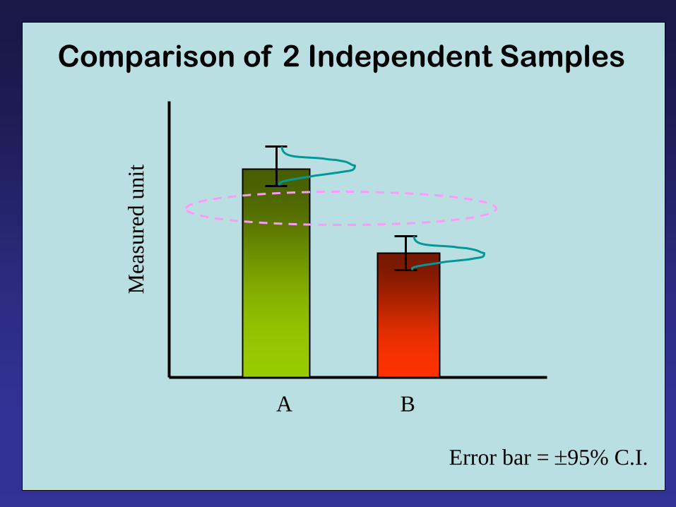
A B
Mea
sure
d u
nit
Comparison of 2 Independent Samples
Error bar = 95% C.I.
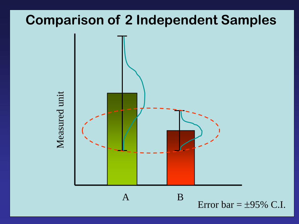
A B
Mea
sure
d u
nit
Comparison of 2 Independent Samples
Error bar = 95% C.I.
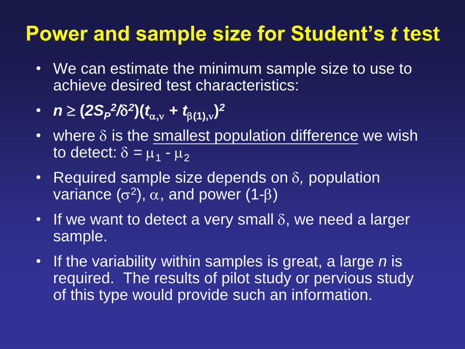
Power and sample size for Student’s t test
• We can estimate the minimum sample size to use to achieve desired test characteristics:
• n (2SP2/2)(t, + t(1),)
2
• where is the smallest population difference we wish to detect: = 1 - 2
• Required sample size depends on , population variance (2), , and power (1-)
• If we want to detect a very small , we need a larger sample.
• If the variability within samples is great, a large n is required. The results of pilot study or pervious study of this type would provide such an information.
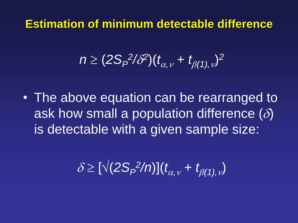
Estimation of minimum detectable difference
n (2SP2/2)(t, + t(1),)
2
• The above equation can be rearranged to
ask how small a population difference ()
is detectable with a given sample size:
[(2SP2/n)](t, + t(1),)
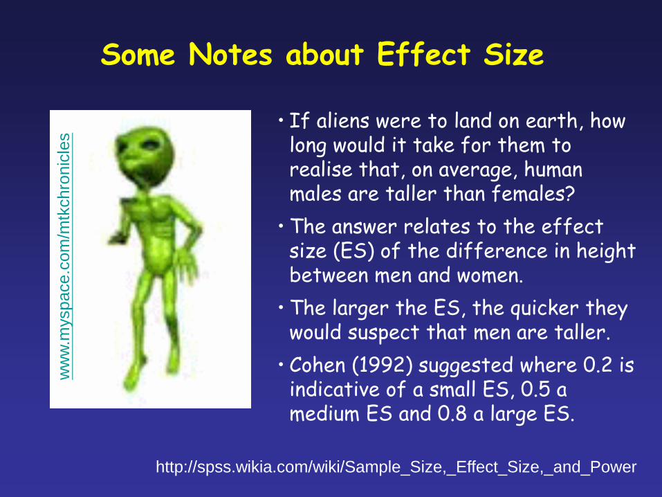
• If aliens were to land on earth, how long would it take for them to realise that, on average, human males are taller than females?
• The answer relates to the effect size (ES) of the difference in height between men and women.
• The larger the ES, the quicker they would suspect that men are taller.
• Cohen (1992) suggested where 0.2 is indicative of a small ES, 0.5 a medium ES and 0.8 a large ES.
Some Notes about Effect Size
http://spss.wikia.com/wiki/Sample_Size,_Effect_Size,_and_Power
ww
w.m
yspace.c
om
/mtk
chro
nic
les
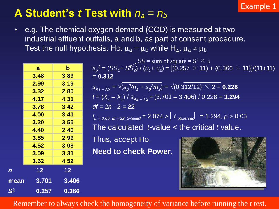
A Student’s t Test with na = nb
• e.g. The chemical oxygen demand (COD) is measured at two
industrial effluent outfalls, a and b, as part of consent procedure.
Test the null hypothesis: Ho: a = b while HA: a b
a b
3.48 3.89
2.99 3.19
3.32 2.80
4.17 4.31
3.78 3.42
4.00 3.41
3.20 3.55
4.40 2.40
3.85 2.99
4.52 3.08
3.09 3.31
3.62 4.52
n 12 12
mean 3.701 3.406
S2 0.257 0.366
sp2 = (SS1+ SS2) / (υ1+ υ2) = [(0.257 × 11) + (0.366 × 11)]/(11+11)
= 0.312
sX1 – X2 = √(sp2/n1 + sp
2/n2) = √(0.312/12) × 2 = 0.228
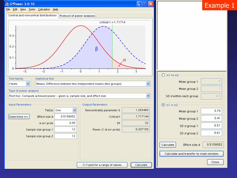
t = (X1 – X2) / sX1 – X2 = (3.701 – 3.406) / 0.228 = 1.294
df = 2n - 2 = 22
t = 0.05, df = 22, 2-tailed = 2.074 > t observed = 1.294, p > 0.05
The calculated t-value < the critical t value.
Thus, accept Ho.
Need to check Power.
SS = sum of square = S2 × υ
Remember to always check the homogeneity of variance before running the t test.
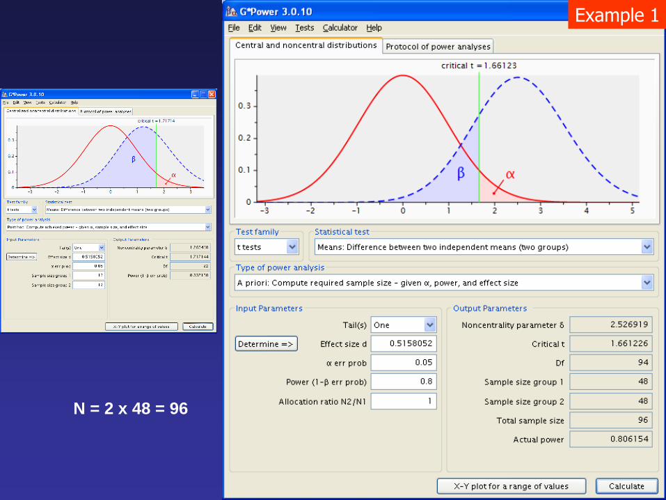
Example 1
Example 1
Example 1
N = 2 x 48 = 96
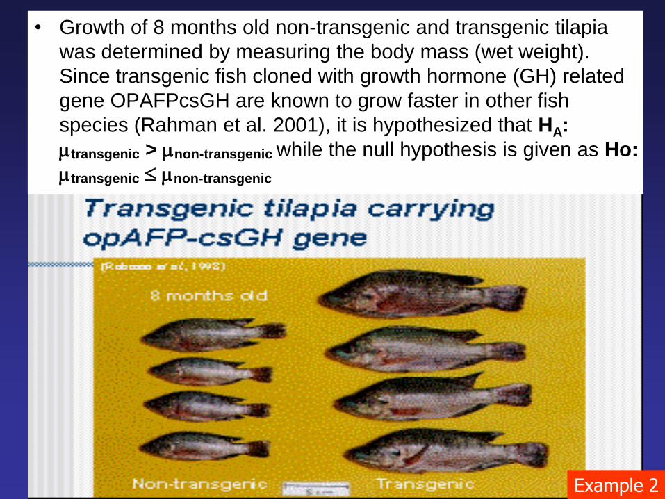
• Growth of 8 months old non-transgenic and transgenic tilapia
was determined by measuring the body mass (wet weight).
Since transgenic fish cloned with growth hormone (GH) related
gene OPAFPcsGH are known to grow faster in other fish
species (Rahman et al. 2001), it is hypothesized that HA:
transgenic > non-transgenic while the null hypothesis is given as Ho:
transgenic non-transgenic
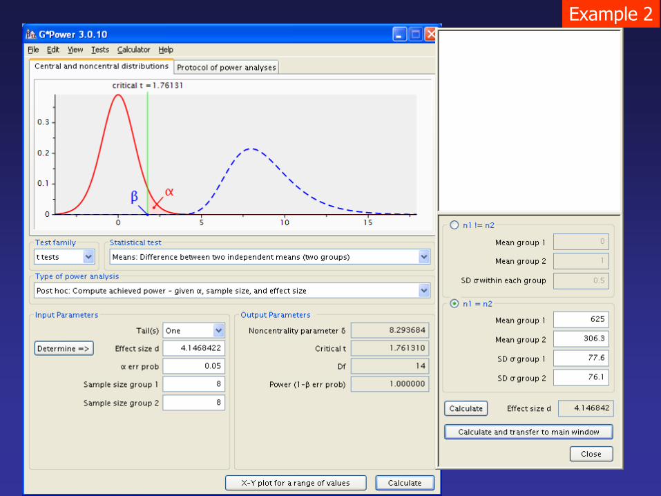
Example 2
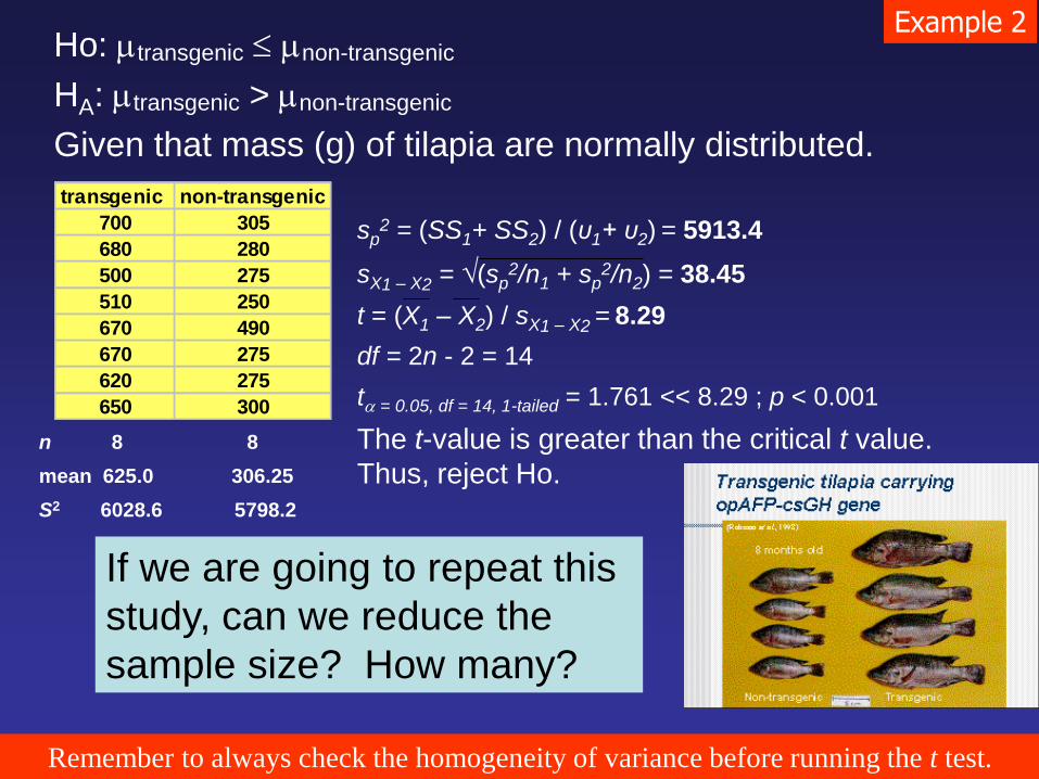
Ho: transgenic non-transgenic
HA: transgenic > non-transgenic
Given that mass (g) of tilapia are normally distributed.
n 8 8
mean 625.0 306.25
S2 6028.6 5798.2
transgenic non-transgenic
700 305
680 280
500 275
510 250
670 490
670 275
620 275
650 300
sp2 = (SS1+ SS2) / (υ1+ υ2) = 5913.4
sX1 – X2 = √(sp2/n1 + sp
2/n2) = 38.45
t = (X1 – X2) / sX1 – X2 = 8.29
df = 2n - 2 = 14
t = 0.05, df = 14, 1-tailed = 1.761 << 8.29 ; p < 0.001
The t-value is greater than the critical t value.
Thus, reject Ho.
Remember to always check the homogeneity of variance before running the t test.
Example 2
If we are going to repeat this
study, can we reduce the
sample size? How many?
Example 2
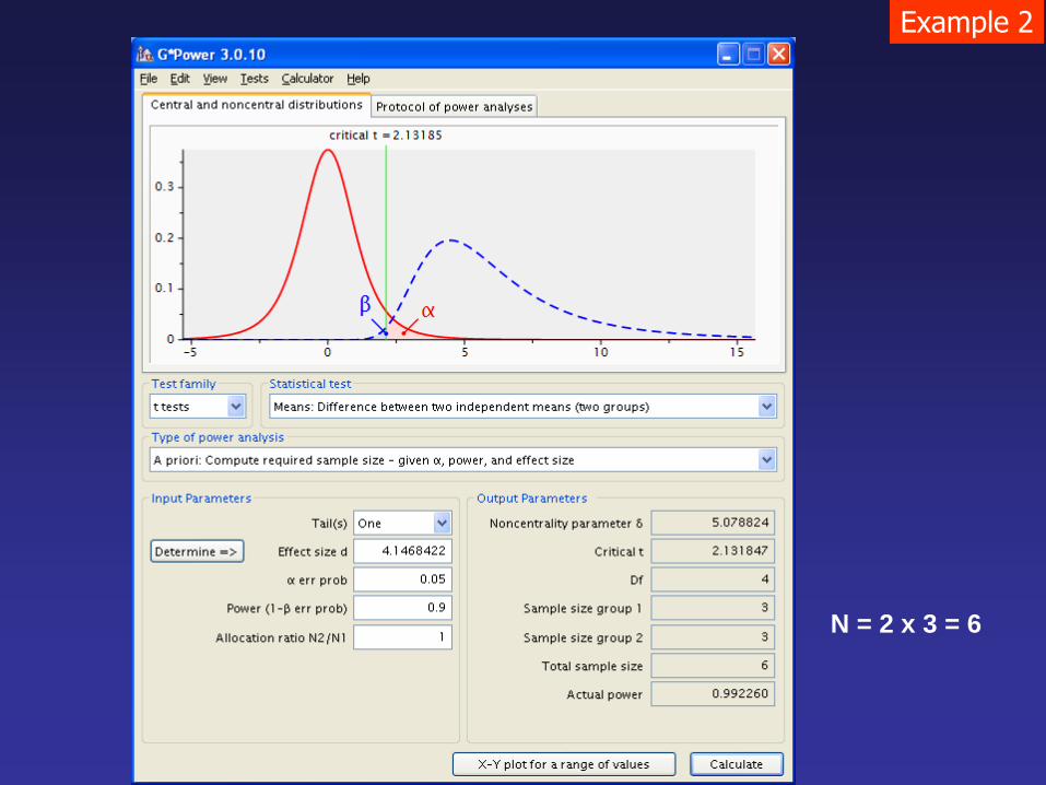
Example 2
N = 2 x 3 = 6
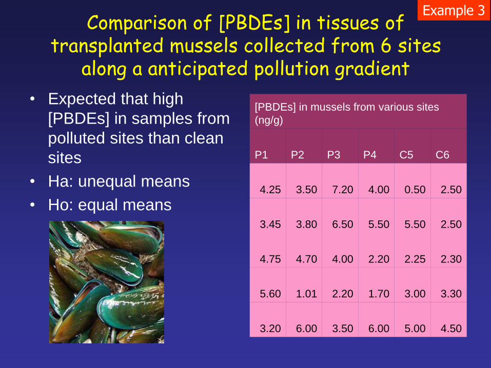
Comparison of [PBDEs] in tissues of transplanted mussels collected from 6 sites
along a anticipated pollution gradient
• Expected that high
[PBDEs] in samples from
polluted sites than clean
sites
• Ha: unequal means
• Ho: equal means
[PBDEs] in mussels from various sites
(ng/g)
P1 P2 P3 P4 C5 C6
4.25 3.50 7.20 4.00 0.50 2.50
3.45 3.80 6.50 5.50 5.50 2.50
4.75 4.70 4.00 2.20 2.25 2.30
5.60 1.01 2.20 1.70 3.00 3.30
3.20 6.00 3.50 6.00 5.00 4.50
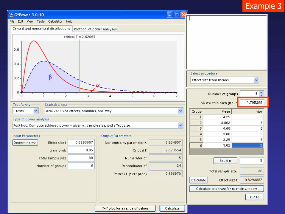
Example 3
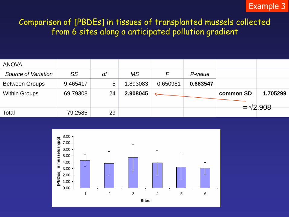
ANOVA
Source of Variation SS df MS F P-value
Between Groups 9.465417 5 1.893083 0.650981 0.663547
Within Groups 69.79308 24 2.908045 common SD 1.705299
Total 79.2585 29
Example 3
Comparison of [PBDEs] in tissues of transplanted mussels collected from 6 sites along a anticipated pollution gradient
0.00
1.00
2.00
3.00
4.00
5.00
6.00
7.00
8.00
1 2 3 4 5 6
Sites
[PB
DE
s]
in m
ussels
(n
g/g
)
= 2.908
Example 3
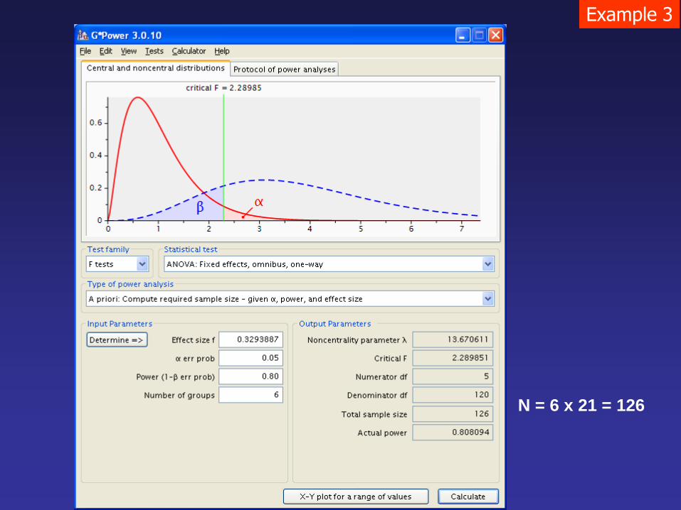
Example 3
N = 6 x 21 = 126
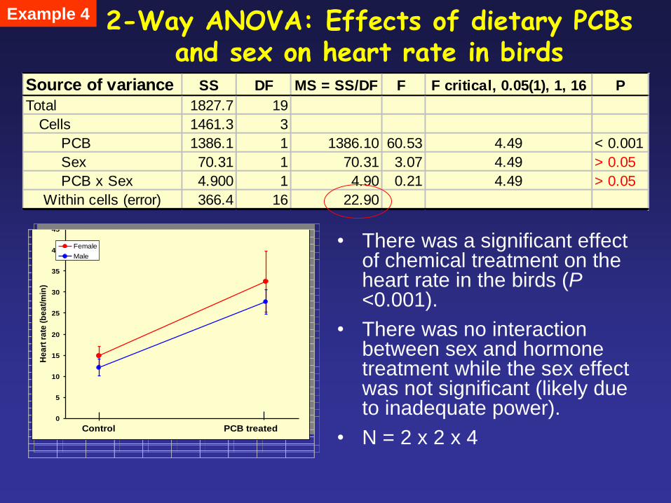
2-Way ANOVA: Effects of dietary PCBs and sex on heart rate in birds
• There was a significant effect of chemical treatment on the heart rate in the birds (P <0.001).
• There was no interaction between sex and hormone treatment while the sex effect was not significant (likely due to inadequate power).
• N = 2 x 2 x 4
Source of variance SS DF MS = SS/DF F F critical, 0.05(1), 1, 16 P
Total 1827.7 19
Cells 1461.3 3
PCB 1386.1 1 1386.10 60.53 4.49 < 0.001
Sex 70.31 1 70.31 3.07 4.49 > 0.05
PCB x Sex 4.900 1 4.90 0.21 4.49 > 0.05
Within cells (error) 366.4 16 22.90
0
5
10
15
20
25
30
35
40
45
He
art
ra
te (
be
at/
min
)
Female
Male
Control PCB treated
Example 4
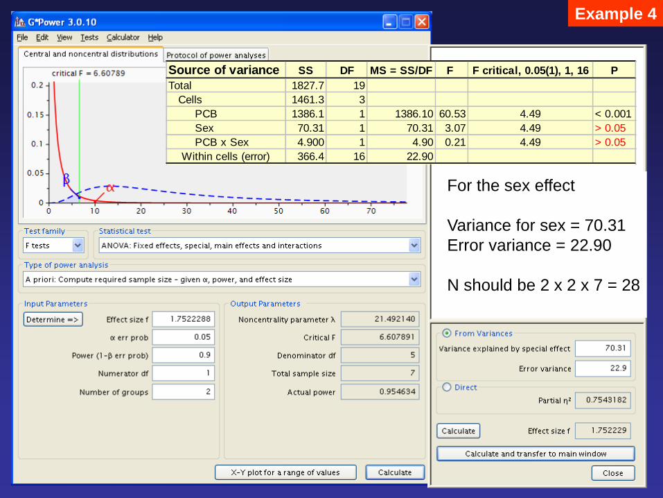
Source of variance SS DF MS = SS/DF F F critical, 0.05(1), 1, 16 P
Total 1827.7 19
Cells 1461.3 3
PCB 1386.1 1 1386.10 60.53 4.49 < 0.001
Sex 70.31 1 70.31 3.07 4.49 > 0.05
PCB x Sex 4.900 1 4.90 0.21 4.49 > 0.05
Within cells (error) 366.4 16 22.90
For the sex effect
Variance for sex = 70.31
Error variance = 22.90
N should be 2 x 2 x 7 = 28
Example 4
Normality Check
Frequency histogram
(Skewness & Kurtosis)
Probability plot, K-S
test
Descriptive
statistics
Measurements
(data)
Mean, SD, SEM,
95% confidence
interval
YES
Check the
Homogeneity
of Variance
Data transformation
NO
Data transformation
NO
Median, range,
Q1 and Q3
Non-Parametric
Test(s)
For 2 samples: Mann-
Whitney
For 2-paired samples:
Wilcoxon
For >2 samples:
Kruskal-Wallis
Sheirer-Ray-Hare
Parametric Tests
Student’s t tests for
2 samples; ANOVA
for 2 samples; post
hoc tests for
multiple comparison
of means
YES
Alternatives to Hypothesis
testing exist
Due to
shortcomings of
inferential stats

There are problems in the conventional hypothesis testing:
http://www.youtube.com/watch?v=ez4DgdurRPg

YouTube - Bayes' Formula
http://www.youtube.com/watch?v=pPTLK5hF
GnQ&feature=channel
By bionicturtledotcom

YouTube - Bayes' Theorem -
Part 2
http://www.youtube.com/watch?v=bcALcVmLva8&feature=related
By westofvideo
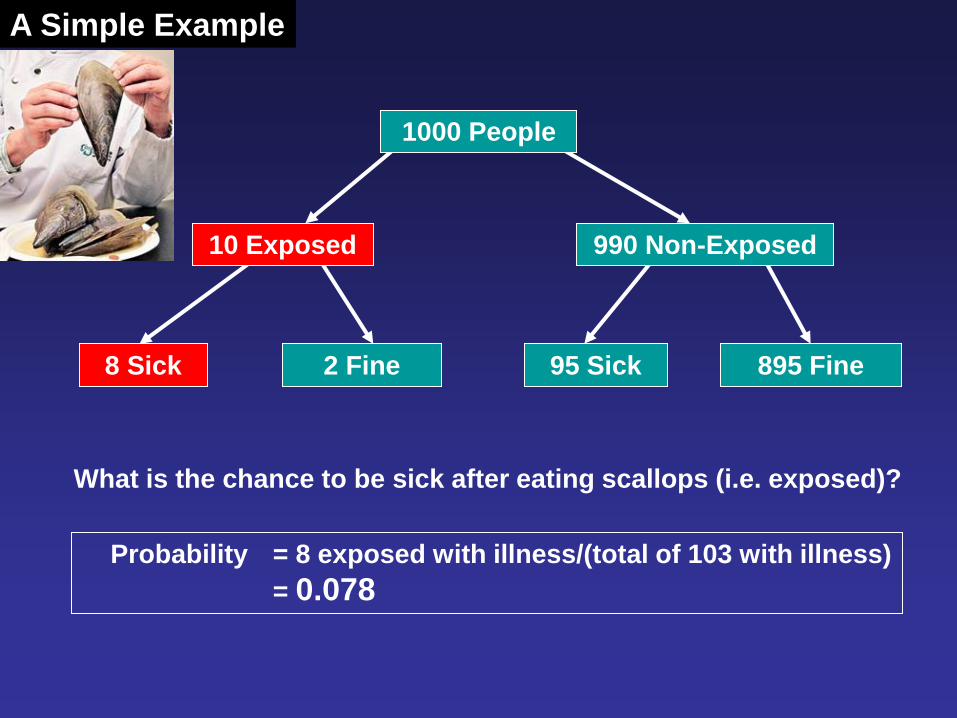
8 Sick 2 Fine 95 Sick 895 Fine
10 Exposed
1000 People
990 Non-Exposed
What is the chance to be sick after eating scallops (i.e. exposed)?
Probability = 8 exposed with illness/(total of 103 with illness)
= 0.078
A Simple Example
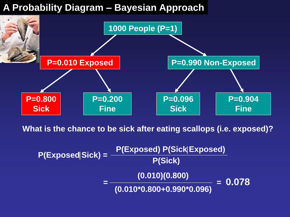
P=0.800
Sick
P=0.200
Fine
P=0.096
Sick
P=0.904
Fine
P=0.010 Exposed
1000 People (P=1)
P=0.990 Non-Exposed
What is the chance to be sick after eating scallops (i.e. exposed)?
A Probability Diagram – Bayesian Approach
P(ExposedSick) = P(Exposed) P(SickExposed)
P(Sick)
= (0.010)(0.800)
(0.010*0.800+0.990*0.096) = 0.078
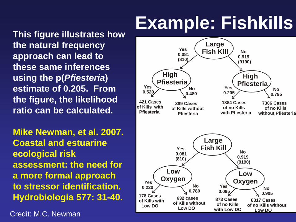
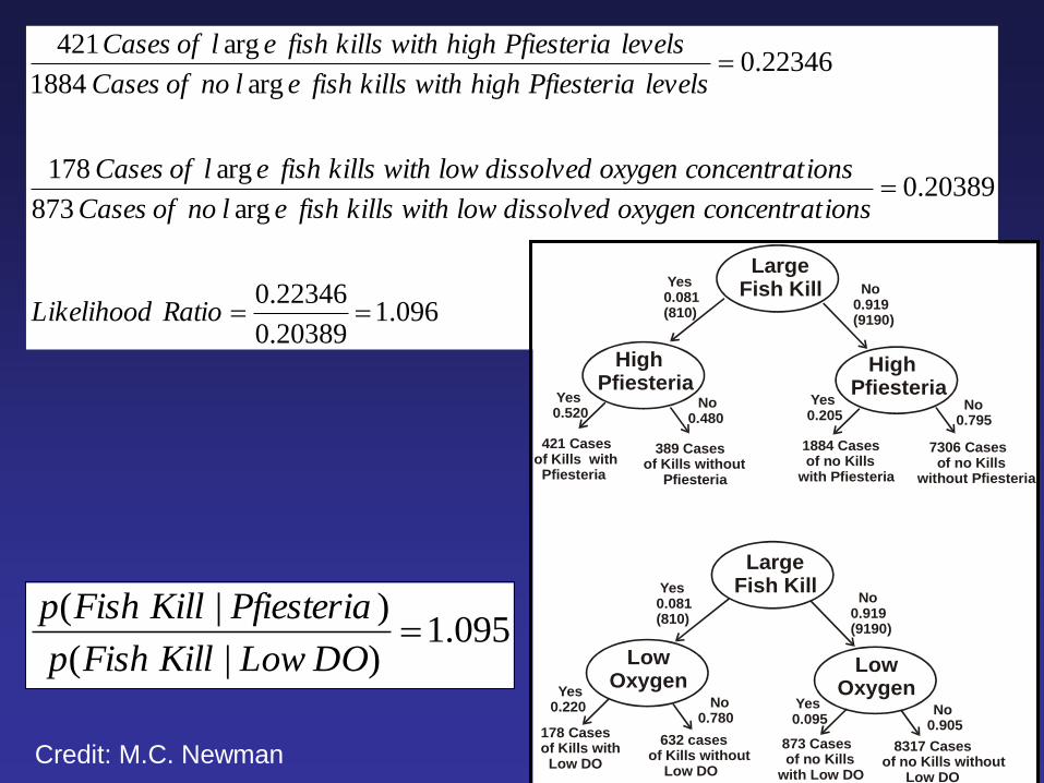
This figure illustrates how
the natural frequency
approach can lead to
these same inferences
using the p(Pfiesteria)
estimate of 0.205. From
the figure, the likelihood
ratio can be calculated.
Mike Newman, et al. 2007.
Coastal and estuarine
ecological risk
assessment: the need for
a more formal approach
to stressor identification.
Hydrobiologia 577: 31-40.
LargeFish Kill
HighPfiesteria
HighPfiesteria
LargeFish Kill
LowOxygen
LowOxygen
Yes0.081(810)
No0.919(9190)
Yes0.520
No0.480
Yes0.205
No0.795
421 Casesof Kills with Pfiesteria
389 Casesof Kills without Pfiesteria
1884 Cases of no Kills with Pfiesteria
7306 Cases of no Kills without Pfiesteria
Yes0.081(810)
No0.919(9190)
Yes0.220 No
0.780 Yes0.095
No0.905
178 Casesof Kills with Low DO
632 casesof Kills without Low DO
873 Cases of no Killswith Low DO
8317 Casesof no Kills without Low DO
Example: Fishkills
Credit: M.C. Newman
096.120389.0
22346.0
20389.0arg873
arg178
22346.0arg1884
arg421
RatioLikelihood
ionsconcentratoxygendissolvedlowwithkillsfishelnoofCases
ionsconcentratoxygendissolvedlowwithkillsfishelofCases
levelsPfiesteriahighwithkillsfishelnoofCases
levelsPfiesteriahighwithkillsfishelofCases
095.1)|(
)|(
DOLowKillFishp
PfiesteriaKillFishp
LargeFish Kill
HighPfiesteria
HighPfiesteria
LargeFish Kill
LowOxygen
LowOxygen
Yes0.081(810)
No0.919(9190)
Yes0.520
No0.480
Yes0.205
No0.795
421 Casesof Kills with Pfiesteria
389 Casesof Kills without Pfiesteria
1884 Cases of no Kills with Pfiesteria
7306 Cases of no Kills without Pfiesteria
Yes0.081(810)
No0.919(9190)
Yes0.220 No
0.780 Yes0.095
No0.905
178 Casesof Kills with Low DO
632 casesof Kills without Low DO
873 Cases of no Killswith Low DO
8317 Casesof no Kills without Low DO
Credit: M.C. Newman
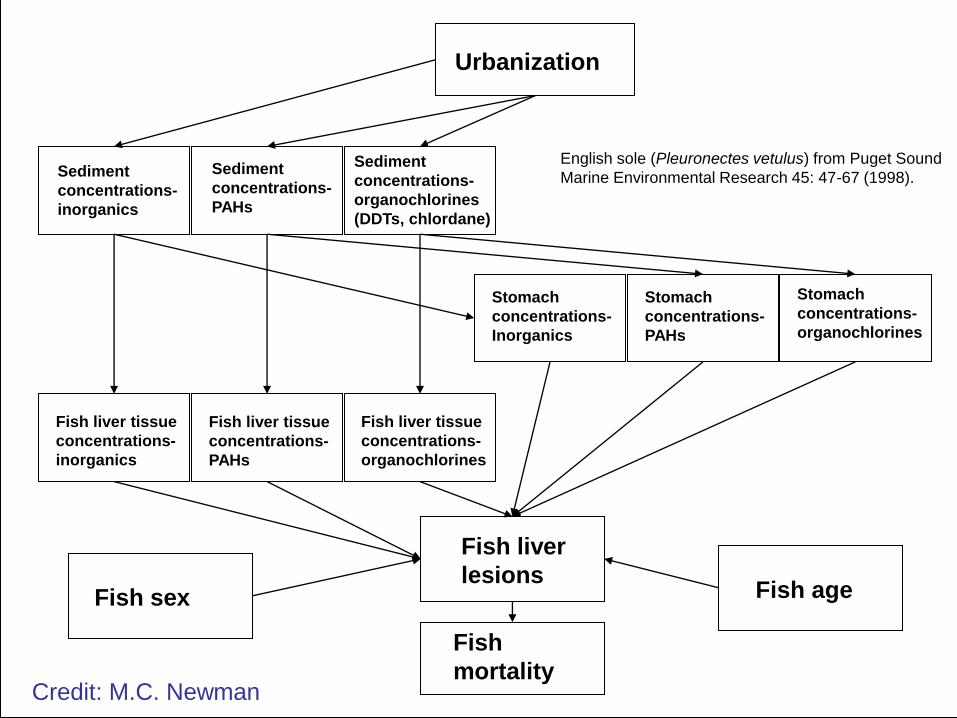
Fish age Fish sex
Urbanization
Fish liver
lesions
Sediment
concentrations-
inorganics
Fish
mortality
Sediment
concentrations-
organochlorines
(DDTs, chlordane)
Sediment
concentrations-
PAHs
Stomach
concentrations-
Inorganics
Stomach
concentrations-
PAHs
Stomach
concentrations-
organochlorines
Fish liver tissue
concentrations-
inorganics
Fish liver tissue
concentrations-
PAHs
Fish liver tissue
concentrations-
organochlorines
English sole (Pleuronectes vetulus) from Puget Sound
Marine Environmental Research 45: 47-67 (1998).
Credit: M.C. Newman
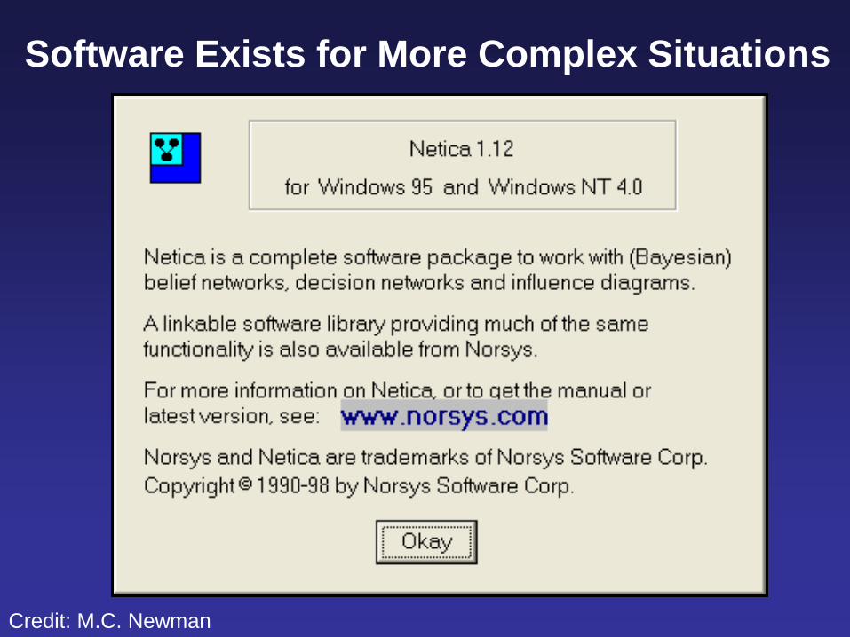
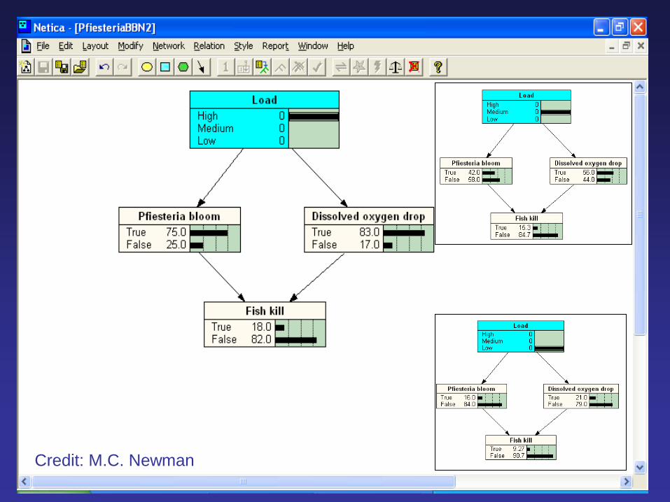
Software Exists for More Complex Situations
Credit: M.C. Newman
Credit: M.C. Newman
Supplemental Readings Aven, T. & J.T. Kvaløy, 2002. Implementing the Bayesian paradigm in risk analysis.
Reliability Engineering and System Safety 78: 195-201.
Bacon, P.J., J.D. Cain & D.C. Howard, 2002. Belief network models of land manager
decisions and land use change. Journal of Environmental Management 65: 1-23.
Belousek, D.W., 2004. Scientific consensus and public policy: the case of Pfiesteria.
Journal Philosophy, Science & Law 4: 1-33.
Borsuk, M.E., 2004. Predictive assessment of fish health and fish kills in the Neuse
River estuary using elicited expert judgment, Human and Ecological Assessment
10: 415-434.
Borsuk, M.E., D. Higdon, C.A. Stow & K.H. Reckhow, 2001. A Bayesian hierarchical
model to predict benthic oxygen demand from organic matter loading in estuaries
and coastal zones. Ecological Modelling 143: 165-181.
Garbolino, P. and F. Taroni. 2002. Evaluation of scientific evidence using Bayesian
networks. Forensic Sci Intern. 125:149-155.
Newman, M.C. and D. Evans. 2002. Causal inference in risk assessments: Cognitive
idols or Bayesian theory? In: Coastal and Estuarine Risk Assessment. CRC Press
LLC, Boca Raton, FL, pp. 73-96.
Newman, M.C., Zhao, Y., and J.F. Carriger. 2007. Coastal and estuarine ecological
risk assessment: the need for a more formal approach to stressor identification.
Hydrobiologia 577: 31-40.
Uusitalo, L. 2007. Advantages and challenges of Bayesian networks in environmental
modeling. Ecol. Modelling 203:312-318.
Credit: M.C. Newman
YouTube - Bayes' Theorem
Introduction
http://www.youtube.com/watch?v=0NGmrwu_BkY&feature=related
By westofvideo
Error Type (Type I & II)
http://www.youtube.com/watch?v=taEmnrTxuzo&feature=related
By bionicturtledotcom