Kendall’s tau and Spearman’s rho - arXiv · Kendall’s tau and Spearman’s rho Manuela...

arXiv: arXiv:0000.0000

On the exact region determined by

Kendall’s tau and Spearman’s rho

Manuela Schreyer, Roland Paulin∗ and Wolfgang Trutschnig†

Department for MathematicsUniversity of SalzburgHellbrunnerstrasse 34

A-5020 Salzburge-mail: [email protected]

[email protected]

[email protected]

Abstract: Using properties of shuffles of copulas and tools from combina-torics we solve the open question about the exact region Ω determined byall possible values of Kendall’s τ and Spearman’s ρ. In particular, we provethat the well-known inequality established by Durbin and Stuart in 1951 isonly sharp on a countable set with sole accumulation point (−1,−1), givea simple analytic characterization of Ω in terms of a continuous, strictlyincreasing piecewise concave function, and show that Ω is compact and sim-ply connected but not convex. The results also show that for each (x, y) ∈ Ωthere are mutually completely dependent random variables whose τ and ρvalues coincide with x and y respectively.

Primary 62H20, 60E15; secondary 28D05, 05A05.Keywords and phrases: Measures of association, Kendall τ , Spearmanρ, Copula, complete dependence.

1. Introduction

Kendall’s τ and Spearman’s ρ are, without doubt, the two most famous non-parametric measures of association/concordance. Given random variables X,Ywith continuous distribution functions F and G respectively, Spearman’s ρ isdefined as the Pearson correlation coefficient of the U(0, 1)-distributed randomvariables U := F X and V := G Y whereas Kendall’s τ is given by theprobability of concordance minus the probability of discordance, i.e.

ρ(X,Y ) = 12(E(UV )− 1

4

)τ(X,Y ) = P

((X1 −X2)(Y1 − Y2) > 0)− P

((X1 −X2)(Y1 − Y2) < 0

),

whereby (X1, Y1) and (X2, Y2) are independent and have the same distributionas (X,Y ). Since both measures are scale invariant they only depend on the

∗Supported by the Austrian Science Fund (FWF): P24574†corresponding author

1

arX

iv:1

502.

0462

0v1

[m

ath.

ST]

16

Feb

2015

http://arxiv.org/abs/arXiv:0000.0000

mailto:[email protected]

Schreyer, Paulin, Trutschnig/On the exact τ -ρ region 2

underlying (uniquely determined) copula A of (X,Y ). It is well known andstraightforward to verify (see [13]) that, given the copula A of (X,Y ), Kendall’sτ and Spearman’s ρ can be expressed as

τ(X,Y ) = 4

∫[0,1]2

A(x, y) dµA(x, y)− 1 =: τ(A) (1.1)

ρ(X,Y ) = 12

∫[0,1]2

xy dµA(x, y)− 3 =: ρ(A), (1.2)

whereby µA denotes the doubly stochastic measure corresponding to A. Con-sidering that τ and ρ quantify different aspects of the underlying dependencestructure (see [6] and the references therein) a very natural question is howmuch they can differ, i.e. if τ(X,Y ) is known which values may ρ(X,Y ) assumeand vice versa. The following well-known universal inequalities between τ andρ go back to Daniels [1] and Durbin and Stuart [4] respectively (for alternativeproofs see [10, 7, 13]):

|3τ − 2ρ| ≤ 1 (1.3)

(1 + τ)2

2− 1 ≤ ρ ≤ 1− (1− τ)2

2(1.4)

The inequalities together yield the set Ω0 (see Figure 1) to which we will referto as classical τ -ρ region in the sequel. Daniels’ inequality is known to be sharp(see [13]) whereas the first part of the inequality by Durbin and Stuart is onlyknown to be sharp at the points pn = (−1+ 2

n ,−1+ 2n2 ) with n ≥ 2 (which, using

symmetry, is to say that the second part is sharp at the points −pn). Althoughboth inequalities are known since the 1950s and the interrelation between τ andρ has received much attention also in recent years (see [6] and the referencestherein), to the best of the authors’ knowledge the exact τ -ρ region Ω, definedby (C denoting the family of all two-dimensional copulas)

Ω =

(τ(X,Y ), ρ(X,Y )) : X,Y continuous random variables

(1.5)

=

(τ(A), ρ(A)) : A ∈ C,

is still unknown.In this paper we give a full characterization of Ω. We derive a piecewise

concave, strictly increasing, continuous function Φ : [−1, 1] → [−1, 1] and (seeTheorem 3.5 and Theorem 5.1) prove that

Ω =

(x, y) ∈ [−1, 1]2 : Φ(x) ≤ y ≤ −Φ(−x). (1.6)

Figure 1 depicts Ω0 and the function Φ (lower red line), the explicit form of Φis given in eq. (3.8) and eq. (3.7). As byproduct we get that the inequality byDurbin and Stuart is not sharp outside the aforementioned points pn and −pn,that Ω is compact and simply connected, but not convex. Moreover, we provethe surprising fact that for each point (x, y) ∈ Ω there exist mutually completelydependent random variables X,Y for which (τ(X,Y ), ρ(X,Y )) = (x, y) holds.


−1.0

−0.5

0.0

0.5

1.0

−1.0 −0.5 0.0 0.5 1.0τ

ρ

Fig 1. The classical τ -ρ-region Ω0 and some copulas (distributing mass uniformly on the bluesegments) for which the inequality by Durbin and Stuart is sharp. The red line depicts thetrue boundary of Ω.

The rest of the paper is organized as follows: Section 2 gathers some notationsand preliminaries. In Section 3 we reduce the problem of determining Ω to aproblem about so-called shuffles of copulas, prove some properties of shufflesand derive the function Φ. The main result saying that Ω is contained in theright-hand-side of eq. (1.6) is given in Section 4, tedious calculations neededfor the proofs are collected to the Appendix. Finally, Section 5 serves to proveequality in eq. (1.6), and to collect some interesting consequences of this result.

2. Notation and Preliminaries

As already mentioned before, C will denote the family of all two-dimensionalcopulas, see [3, 5, 13, 16]. M and W will denote the minimum copula and thelower Frechet-Hoeffding bound respectively. Given A ∈ C the transpose At ∈ Cof A is defined by At(x, y) := A(y, x) for all x, y ∈ [0, 1]. d∞ will denote theuniform distance on C; it is well known that (C, d∞) is a compact metric spaceand that d∞ is a metrization of weak convergence in C. For every A ∈ C thecorresponding doubly stochastic measure will be denoted by µA, i.e. we haveµA([0, x] × [0, y]) := A(x, y) for all x, y ∈ [0, 1]. PC denotes the class of all

these doubly stochastic measures. B([0, 1]) and B([0, 1]2) will denote the Borelσ-fields in [0, 1] and [0, 1]2, λ and λ2 the Lebesgue measure on [0, 1] and [0, 1]2

respectively. Instead of λ-a.e. we will simply write a.e. since no confusion willarise. T will denote the class of all λ-preserving transformations h : [0, 1] →[0, 1], i.e. transformations for which the push-forward λh of λ via h coincideswith λ, Tb the subclass of all bijective h ∈ T .

For every copula A ∈ C there exists a Markov kernel (regular conditionaldistribution) KA : [0, 1]× B([0, 1])→ [0, 1] fulfilling (Gx := y ∈ [0, 1] : (x, y) ∈G denoting the x-section of G ∈ B([0, 1]2) for every x ∈ [0, 1])∫

[0,1]

KA(x,Gx) dλ(x) = µA(G), (2.1)

for every G ∈ B([0, 1]2), so, in particular∫[0,1]

KA(x, F ) dλ(x) = λ(F ) (2.2)

for every F ∈ B([0, 1]). We will refer to KA simply as Markov kernel of A. Onthe other hand, every Markov kernel K : [0, 1]×B([0, 1])→ [0, 1] fulfilling (2.2)induces a unique element µ ∈ PC([0, 1]2) via (2.1). For more details and prop-erties of regular conditional distributions and disintegration we refer to [8, 9].A copula A ∈ C will be called completely dependent if and only if there existsh ∈ T such that K(x,E) := 1E(h(x)) is a Markov kernel of A (see [11, 19] forequivalent definitions and main properties). For every h ∈ T the induced com-pletely dependent copula will be denoted by Ah. Note that h1 = h2 a.e. impliesAh1

= Ah2and that eq. (2.1) implies Ah(x, y) = λ([0, x] ∩ h−1([0, y])) for all

x, y ∈ [0, 1]. In the sequel Cd will denote the family of all completely dependentcopulas. Ah ∈ Cd will be called mutually completely dependent if we even haveh ∈ Tb. Note that in case of h ∈ Tb we have Ah−1 = (Ah)t. Complete depen-dence is the exact opposite of independence since it describes the (not necessar-ily mutual) situation of full predictability/maximum dependence. Some notionsquantifying dependence of two-dimensional random variables which, contraryto Schweizer and Wolff’s σ (see [15]) are not based on d∞ have been studied in[18, 19].

Tackling the problem of determining the region Ω, our main tool will bespecial members of the class Cd usually referred to as shuffles of the minimumcopula M . Following [13] we will call h ∈ Tb a shuffle (and Ah ∈ Cd a shuffle ofM) if there exist 0 = s0 < s1 < . . . < sn−1 < sn = 1 and ε = (ε1, . . . , εn) ∈−1, 1n such that we have h′(x) = εi for every x ∈ (si−1, si). In case of εi = 1for every i ∈ 1, . . . , n we will call h straight shuffle. S will denote the family ofall shuffles, S+ the family of all straight shuffles. It is well known (see [12, 13])that CS+ , defined by

CS+ =Ah : h ∈ S+

(2.3)

is dense in (C, d∞). For more general definitions of shuffles we refer to [3]. Ob-viously every shuffle h ∈ S can be expressed in terms of vectors u ∈ ∆n, ε ∈


−1, 1n and a permutation π ∈ σn, whereby ∆n denotes the unit simplex∆n = x ∈ [0, 1]n :

∑ni=1 xi = 1 and σn denotes all bijections on 1, . . . , n. In

fact, choosing suitable u ∈ ∆n, ε ∈ −1, 1n, π ∈ σn, setting (empty sums arezero by definition)

sk :=

k∑i=1

ui, tk :=

k∑i=1

uπ−1(i) (2.4)

for every k ∈ 0, . . . , n, we have sk − sk−1 = uk = tπ(k) − tπ(k)−1 and on(sk−1, sk) the shuffle h is given by

h(x) = hπ,u,ε(x) :=

tπ(k)−1 + x− sk−1 if εk = 1,tπ(k) − (x− sk−1) if εk = −1.

(2.5)

s0 = 0 s1 s2 s3 s4 = 1

t0 = 0

t1

t2

t3

t4 = 1

Fig 2. Shuffle hπ,u,ε with π = (4, 2, 1, 3), u = ( 18, 38, 14, 14

) and ε = (1,−1, 1, 1)

In the sequel we will directly work with the function hπ,u,ε, implicitly defined

in eq. (2.5) since all possible extensions of hπ,u,ε from⋃ki=1(sk−1, sk) to [0, 1]

yield the same copula, which we will denote by Ahπ,u,ε . In case of εi = 1 forevery i ∈ 1, . . . , n we will simply write hπ,u in the sequel. Note that the


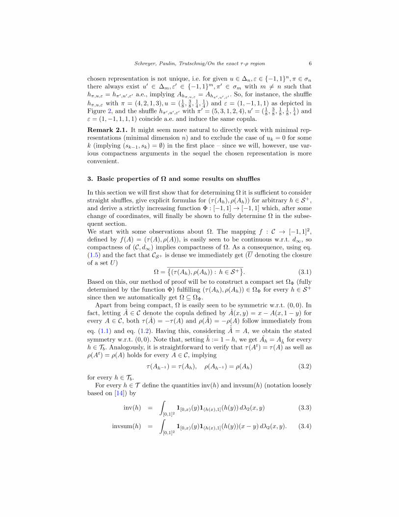
chosen representation is not unique, i.e. for given u ∈ ∆n, ε ∈ −1, 1n, π ∈ σnthere always exist u′ ∈ ∆m, ε

′ ∈ −1, 1m, π′ ∈ σm with m 6= n such thathπ,u,ε = hπ′,u′,ε′ a.e., implying Ahπ,u,ε = Ahπ′,u′,ε′ . So, for instance, the shuffle

hπ,u,ε with π = (4, 2, 1, 3), u = (18 ,

38 ,

14 ,

14 ) and ε = (1,−1, 1, 1) as depicted in

Figure 2, and the shuffle hπ′,u′,ε′ with π′ = (5, 3, 1, 2, 4), u′ = ( 18 ,

38 ,

18 ,

18 ,

14 ) and

ε = (1,−1, 1, 1, 1) coincide a.e. and induce the same copula.

Remark 2.1. It might seem more natural to directly work with minimal rep-resentations (minimal dimension n) and to exclude the case of uk = 0 for somek (implying (sk−1, sk) = ∅) in the first place – since we will, however, use var-ious compactness arguments in the sequel the chosen representation is moreconvenient.

3. Basic properties of Ω and some results on shuffles

In this section we will first show that for determining Ω it is sufficient to considerstraight shuffles, give explicit formulas for (τ(Ah), ρ(Ah)) for arbitrary h ∈ S+,and derive a strictly increasing function Φ : [−1, 1]→ [−1, 1] which, after somechange of coordinates, will finally be shown to fully determine Ω in the subse-quent section.We start with some observations about Ω. The mapping f : C → [−1, 1]2,defined by f(A) = (τ(A), ρ(A)), is easily seen to be continuous w.r.t. d∞, socompactness of (C, d∞) implies compactness of Ω. As a consequence, using eq.(1.5) and the fact that CS+ is dense we immediately get (U denoting the closureof a set U)

Ω =

(τ(Ah), ρ(Ah)) : h ∈ S+. (3.1)

Based on this, our method of proof will be to construct a compact set ΩΦ (fullydetermined by the function Φ) fulfilling (τ(Ah), ρ(Ah)) ∈ ΩΦ for every h ∈ S+

since then we automatically get Ω ⊆ ΩΦ.Apart from being compact, Ω is easily seen to be symmetric w.r.t. (0, 0). In

fact, letting A ∈ C denote the copula defined by A(x, y) = x − A(x, 1 − y) forevery A ∈ C, both τ(A) = −τ(A) and ρ(A) = −ρ(A) follow immediately from

eq. (1.1) and eq. (1.2). Having this, consideringˆA = A, we obtain the stated

symmetry w.r.t. (0, 0). Note that, setting h := 1− h, we get Ah = Ah for everyh ∈ Tb. Analogously, it is straightforward to verify that τ(At) = τ(A) as well asρ(At) = ρ(A) holds for every A ∈ C, implying

τ(Ah−1) = τ(Ah), ρ(Ah−1) = ρ(Ah) (3.2)

for every h ∈ Tb.For every h ∈ T define the quantities inv(h) and invsum(h) (notation loosely

based on [14]) by

inv(h) =

∫[0,1]2

1[0,x)(y)1(h(x),1](h(y)) dλ2(x, y) (3.3)

invsum(h) =

∫[0,1]2

1[0,x)(y)1(h(x),1](h(y))(x− y) dλ2(x, y). (3.4)

Then the following result holds:

Lemma 3.1. For every h ∈ Tb the following relations hold:

τ(Ah) = 4

∫[0,1]

Ah(x, h(x)) dλ(x)− 1 = 1− 4 inv(h)

ρ(Ah) = 12

∫[0,1]

xh(x) dλ(x)− 3 = 1− 12 invsum(h)

Moreover, for every h ∈ Tb we have (inv(h), invsum(h)) ∈[0, 1

2

]×[0, 1

6

].

Proof. Using disintegration we immediately get

τ(Ah) = 4

∫[0,1]

∫[0,1]

Ah(x, y)KAh(x, dy) dλ(x)− 1

= 4

∫[0,1]

Ah(x, h(x)) dλ(x)− 1

as well as

inv(h) =

∫[0,1]

∫[0,x]

(1− 1[0,h(x)](h(y))

)dλ(y)dλ(x)

=

∫[0,1]

(x−Ah(x, h(x))

)dλ(x) =

1− τ(Ah)

4

which proves the first identity. The first part of the second one is an im-mediate consequence of disintegration. To prove the remaining equality use∫

[0,x)1(h(x),1](h(y)) dλ(y) = x − Ah(x, h(x)) and

∫(y,1]

1[0,h(y))(h(x)) dλ(x) =

h(y)−Ah(y, h(y)) to finally get

invsum(Ah) =

∫[0,1]

x(x−Ah(x, h(x))− (h(x)−Ah(x, h(x))

)dλ(x)

=1

3−∫

[0,1]

xh(x) dλ(x).

The fact that (inv(Ah), invsum(Ah)) ∈[0, 1

2

]×[0, 1

6

]is a direct consequence of

Ω ⊆ [−1, 1]2.

As next step we derive explicit formulas for inv(h) and invsum(h) for the caseof h being a straight shuffle based on which we will afterwards derive the afore-mentioned function Φ determining the region Ω. To simplify notation define

Iπ =i, j : 1 ≤ i < j ≤ n, π(i) > π(j)

Qπ =

i, j, k : 1 ≤ i < j < k ≤ n, π(i) > π(j) > π(k) or (3.5)

π(j) > π(k) > π(i) or π(k) > π(i) > π(j),

as well as

aπ(u) = inv(hπ,u), bπ(u) = inv(hπ,u)− 2 invsum(hπ,u) (3.6)

for every π ∈ σn and u ∈ ∆n. The following lemma (the proof of which is givenin the Appendix) holds.

Lemma 3.2. For every (π, u) ∈ σn ×∆n the following identities hold:

inv(hπ,u) = aπ(u) =∑

i<j, i,j∈Iπ

uiuj

invsum(hπ,u) =∑

i<j, i,j∈Iπ

1

2u2iuj +

1

2uiu

2j +

∑k: i<k<j

uiujuk

bπ(u) =

∑i<j<k, i,j,k∈Qπ

uiujuk

As pointed out in the Introduction, the first part of inequality (1.4) is knownto be sharp only at the points pn = (−1 + 2

n ,−1 + 2n2 ) with n ≥ 2. According

to [13] (or directly using Lemma 3.2), considering π = (n, n − 1, . . . , 2, 1) andu1 = u2 = . . . = un = 1

n we get pn = (τ(Ahπ,u), ρ(Ahπ,u)). Having this, it seemsnatural to conjecture that all shuffles of the form Ahπ,u with

π = (n, n− 1, . . . , 2, 1), u1 = u2 = . . . = un−1 = r, un = 1− (n− 1)r

for some n ≥ 2 and r ∈ ( 1n ,

1n−1 ) might also be extremal in the sense that

(τ(Ahπ,u), ρ(Ahπ,u)) is a boundary point of Ω. Main content of the paper is theconfirmation of this very conjecture. We will assign all shuffles of the just men-tioned form the name prototype, calculate τ and ρ explicitly for all prototypesand then, based on these values, derive the function Φ.

Definition 3.3. π ∈ σn will be called decreasing if π = (n, n− 1, . . . , 2, 1). Thepair (π, u) ∈ σn×∆n will be called a prototype if π is decreasing and there existssome r ∈ [ 1

n ,1

n−1 ] such that u1 = u2 = . . . = un−1 = r and un = 1 − (n − 1)r.

Analogously, h ∈ S+ (and Ah ∈ Cd) is called a prototype if there exists aprototype (π, u) such that h = hπ,u a.e.

Using the identities from Lemma 3.2 we get the following expressions forprototypes (the proof is given in the Appendix):

Lemma 3.4. Suppose that (π, u) ∈ σn ×∆n is a prototype, then

τ(Ahπ,u) = 1− 4(n− 1)r + 2r2n(n− 1) ∈[

2−nn , 2−(n−1)

n−1

]ρ(Ahπ,u) = 1− 2r(n− 1)

(3− 3r(n− 1) + r2(n− 2)n

)∈[

2−n2

n2 , 2−(n−1)2

(n−1)2

].

Fix n ≥ 2. Then both functions r 7→ 1 − 4(n − 1)r + 2r2n(n − 1) and r 7→1 − 2r(n − 1)

(3 − 3r(n − 1) + r2(n − 2)n

)are strictly increasing on [ 1

n ,1

n−1 ].Expressing r as function of τ and substituting the result in the expression for ρdirectly yields

ρ(Ahπ,u) = −1− 4

n2+

3

n+

3τ(Ahπ,u)

n− n− 2√

2n2√n− 1

(n− 2 + nτ(Ahπ,u))3/2.


Based on this interrelation define Φn : [−1 + 2n , 1]→ [−1, 1] by

Φn(x) = −1− 4

n2+

3

n+

3x

n− n− 2√

2n2√n− 1

(n− 2 + nx)3/2 (3.7)

and set

Φ(x) =

−1 if x = −1,

Φn(x) if x ∈[

2−nn , 2−(n−1)

n−1

]for some n ≥ 2.

(3.8)

Since we have Φn( 2−nn ) = Φn+1( 2−n

n ) = −1 + 2n2 for every n ≥ 1 this defines

a function Φ : [−1, 1] → [−1, 1]. Notice that Φ2(x) = − 12 + 3x

2 , i.e. on [0, 1]Φ coincides with Daniels’ linear bound and for xn = 2−n

n and n ≥ 2 we have(xn,Φ(xn)) = pn, i.e. (xn,Φ(xn)) coincides with the points at which Durbin andStuart’s inequality is known to be sharp. Furthermore, it is straightforward toverify that Φ is a strictly increasing homemorphism on [−1, 1] which is concave

on every interval [ 2−nn , 2−(n−1)

n−1 ] with n ≥ 2. Figure 3 depicts the function Φ aswell as some prototypes and their corresponding Kendall’s τ and Spearman’s ρ.Defining the compact set ΩΦ by

ΩΦ =

(x, y) ∈ [−1, 1]2 : Φ(x) ≤ y ≤ −Φ(−x), (3.9)

we can now state the following main result the proof of which is given in thenext section.

Theorem 3.5. The precise τ -ρ region Ω fulfills Ω ⊆ ΩΦ.

Remark 3.6. The fact that Ω ⊆ ΩΦ holds is the principal result of this papersince it improves the classical inequality by Durbin and Stuart mentioned in theIntroduction and, more importantly, gives sharp bounds everywhere. In Section5 we will, however, show that even Ω = ΩΦ holds and that for every point(x, y) ∈ Ω there exists a shuffle h ∈ S such that (τ(Ah), ρ(Ah)) = (x, y).

Remark 3.7. A function similar (but not identical) to Φ has appeared inthe literature in [17], where the authors tried to deduce sharp bounds of Ω byrunning simulations (but did not provide any analytic proof). Additionally, ithas been brought to our attention during the preparation of this manuscript thatManuel Ubeda-Flores (University of Almerıa) already conjectured Theorem 3.5(with the exact form of Φ) in a working paper in 2009.

4. Proof of the main theorem

Using the properties of Ω mentioned at the beginning of Section 3, Theorem3.5 is proved if we can show that for every h ∈ S+ we have ρ(Ah) ≥ Φ(τ(Ah)).Given Lemma 3.2 it is straightforward to verify that this is equivalent to showinginvsum(h) ≤ ϕ(inv(h)) for every h ∈ S+ whereby ϕ : [0, 1

2 ] → [0, 16 ] is defined

by

ϕ(x) =

16 if x = 1

2 ,ϕn(x) if x ∈ [ 1

2 −1

2(n−1) ,12 −

12n ] for some n ≥ 2

(4.1)


−1.0

−0.9

−0.8

−0.7

−0.6

−0.5

−0.6 −0.4 −0.2 0.0τ

ρ

Fig 3. The function Φ (red) and some prototypes with their corresponding Kendall’s τ andSpearman’s ρ. The shaded region depicts the classical τ -ρ-region Ω0, straight lines connectingthe points pn are plotted in green.

and ϕn : [ 12 −

12(n−1) ,

12 −

12n ]→ [0, 1

6 ] is given by

ϕn(x) =1

6+

1

3n2− 1

2n+x

n+

n− 2

6n2√n− 1

(n− 1− 2nx)3/2. (4.2)

Translating this to aπ(u) and bπ(u), using eq. (3.6) and defining ϑ : [0, 12 ]→ [0, 1

6 ]by ϑ(x) = x− 2ϕ(x) we arrive at the following equivalent form of Theorem 3.5:

Theorem 4.1. For every n ∈ N, π ∈ σn and u ∈ ∆n the following inequalityholds:

bπ(u) ≥ ϑ(aπ(u)) (4.3)

We are now going to prove this result and start with some first observationsand an outline of the structure of the subsequent proof. (i) ϑ is continuousand, by calculating the derivative, it is straightforward to see that ϑ is non-decreasing. (ii) ϑ(0) = ϑ( 1

4 ) = 0 and ϑ( 12 ) = 1

6 . (iii) For every prototype (π, u)we have equality bπ(u) = ϑ(aπ(u)). (iv) For given n and fixed π ∈ σn the func-tions v 7→ aπ(v) and v 7→ bπ(v) are continuous on ∆n, so there exists some

u ∈ ∆n minimizing the function v 7→ bπ(v) − ϑ(aπ(v)). (v) For n ≤ 2 the in-equality bπ(u) ≥ ϑ(aπ(u)) trivially holds for every π ∈ σn and every u ∈ ∆n, sofrom now on we will only consider the case n ≥ 3.

The structure of the proof of Theorem 4.1 is as follows:

1. Preliminary Step 1: We prove inequality (4.3) for the case of decreasingπ ∈ σn.

2. Preliminary Step 2: We analyze how, for fixed π ∈ σn, the quantities aπ(u)and bπ(u) change if u ∈ ∆n changes.

3. Induction Step 1: Assuming that the result is true for all (π, u) ∈ σm×∆m

with m < n we prove inequality (4.3) for (π, u) ∈ σn × ∆n under thehypothesis that there either exist (i) p < q < r such that π(r) > π(q) >π(p) or (ii) p < q < r < s such that π(q) > π(p) > π(s) > π(r) holds.

4. Induction Step 2: Assuming that the result is true for all (π, u) ∈ σm×∆m

with m < n we prove inequality (4.3) for (π, u) ∈ σn × ∆n with π notfulfilling the hypothesis in Induction Step I.

Preliminary Step 1 : Consider n ≥ 3 and π = (n, n− 1, . . . , 2, 1). Note that inthis situation we have e1(u) = 1, e2(u) = aπ(u), e3(u) = bπ(u) for every u ∈ ∆n,whereby ei denotes the i-th elementary symmetric polynomial for i ∈ 1, 2, 3,i.e. e1(v) :=

∑i vi, e2(v) :=

∑i<j vivj and e3(v) :=

∑i<j<k vivjvk for every

v ∈ Rn. Hence aπ(u) and bπ(u) do not change if we reorder the coordinates ofu.

Lemma 4.2. Suppose that n ≥ 3, π = (n, n − 1, . . . , 2, 1), c2 ∈ aπ(∆n) andthat u ∈ ∆n fulfills bπ(u) = minbπ(v) : v ∈ ∆n ∩ (aπ)−1(c2) as well asu1 ≥ · · · ≥ un ≥ 0. Then there exists m ∈ 1, . . . , n such that ui = 0 for everyi > m, and u1 = · · · = um−1 ≥ um.

Proof. Note that continuity of bπ and compactness of ∆n∩(aπ)−1(c2) impliesthe existence of the minimum. We first prove the statement for the case n =3 and suppose that u is a minimizer fulfilling u3 ≥ u2 ≥ u1 ≥ 0. Define apolynomial f : R→ R by

f(T ) = (T − u1)(T − u2)(T − u3) = T 3 − T 2 + c2T − e3(u),

and let Df denote the discriminant of f . It is well known that Df > 0 if andonly if f has three distinct real zeros and that in case of Df 6= 0 locally thezeros of f are smooth (so in particular continuous) functions of the coefficientsof f .

Suppose that u1 > u2 > u3 > 0. Then Df > 0. Let fε(T ) = T 3 − T 2 +c2T − (e3(u) − ε), then for small enough values of ε > 0, the polynomial fεhas three distinct, positive real zeros: uε,1, uε,2, uε,3. Then uε,1 + uε,2 + uε,3 = 1and uε,1uε,2 + uε,2uε,3 + uε,3uε,1 = c2, while uε,1uε,2uε,3 = e3(u) − ε < e3(u),contradiction. So either u3 = 0 or u1 = u2 or u1 > u2 = u3 > 0. In the firsttwo cases we are done, so suppose that u1 > u2 = u3 > 0. Then 1 = u1 + 2u2

and c2 = 2u1u2 + u22. Suppose that u1 ≥ 4u2. Then 1 ≥ 4c2, so there are

unique y1 ≥ y2 ≥ 0 such that y1 + y2 = 1 and y1y2 = c2. Let y3 = 0, thenconsidering y = (y1, y2, y3) we get e1(y) = 1, e2(y) = c2, and e3(y) = 0 < e3(u),contradiction. So 4u2 > u1 > u2. Let y1 = y2 = 2u1+u2

3 and y3 = 4u2−u1

3 . Theny1, y2, y3 ≥ 0, e1(y) = 1, e2(y) = c2, and e3(y) = 1

27 (2u1 + u2)2(4u2 − u1) =e3(u)− 4

27 (u1 − u2)3 < e3(u), contradiction. This proves the claim for n = 3.Suppose indirectly that the statement is false for some n > 3. Then there

are i < j < k such that ui > uj ≥ uk > 0. Setting ul := ului+uj+uk

for every

l ∈ i, j, k obviously ui + uj + uk = 1. Applying the case n = 3 to ui, uj , ukyields yi, yj , yk ∈ [0, 1] such that yi + yj + yk = ui + uj + uk, yiyj + yj yk +ykyi = uiuj + uj uk + ukui and yiyj yk < uiuj uk. Setting yl = ul for everyl ∈ 1, . . . , n \ i, j, k and yl = yl(ui + uj + uk) for every l ∈ i, j, k finallyyields e1(y) = e1(u), e2(y) = e2(u) and e3(y) < e3(u), contradiction.

Corollary 4.3. Suppose that n ≥ 3 and that π = (n, n − 1, . . . , 2, 1). Thenbπ(u) ≥ ϑ(aπ(u)) holds for every u ∈ ∆n.

Preliminary Step 2 : We investigate how, for fixed π ∈ σn, the quantitiesaπ(u) and bπ(u) change if u ∈ ∆n changes. To do so, temporarily extend aπ andbπ to full Rn using the identities in Lemma 3.2. The following lemmata (whoseproof is given in the Appendix) will be crucial in the sequel.

Lemma 4.4. Suppose that n ≥ 3 and that δ = (δ1, . . . , δn) ∈ Rn fulfills∑i δi =

0. Then for every t ∈ R the following identities hold:

aπ(u+ tδ)− aπ(u) = α1t+ α2t2 (4.4)

bπ(u+ tδ)− bπ(u) = β1t+ β2t2 + β3t

3 (4.5)

whereα1 =

∑i

aiδi, α2 =∑

i<j, i,j∈Iπ

δiδj ,

β1 =∑i

biδi, β2 =∑i<j

ci,jδiδj , β3 =∑

i<j<k,i,j,k∈Qπ

δiδjδk,

and

ai =∑

j: i,j∈Iπ

uj , bi =∑

j<k, i,j,k∈Qπ

ujuk, ci,j = cj,i =∑

k: i,j,k∈Qπ

uk.

Lemma 4.5. Suppose that n ≥ 3 and that π ∈ σn. If p, q, r ∈ 1, . . . , n aredistinct elements such that p, q, r /∈ Qπ, then cp,r + cq,r ≥ cp,q ≥ 0.

We now state two conditions for π that imply the existence of a directionδ ∈ Rn \ 0 with

∑i δi = 0 such that t 7→ aπ(u + tδ) − aπ(u) is identical to

zero for every t and t 7→ bπ(u+ tδ)− bπ(u) is of degree two and concave.

Lemma 4.6. Suppose that n ≥ 3, that π ∈ σn, and that one of the followingtwo conditions holds:

(i) There exist p, q, r ∈ 1, 2, . . . , n with p < q < r and π(r) > π(q) > π(p).

(ii) There exist p, q, r, s ∈ 1, 2, . . . , n with p < q < r < s and π(q) > π(p) >π(s) > π(r).

Then there exists δ ∈ Rn \0 such that the coefficients in (4.4) and (4.5) fulfillα1 = α2 = β3 = 0 and β2 ≤ 0.

Induction Step 1 : We prove the induction step for all π ∈ σn fulfilling one ofthe conditions in Lemma 4.6.

Lemma 4.7. Suppose that n ≥ 3 and that bω(v) ≥ ϑ(aω(v)) holds for all(ω, v) ∈ σm×∆m with m < n. If π ∈ σn fulfills one of the conditions in Lemma4.6 then bπ(u) ≥ ϑ(aπ(u)) for every u ∈ ∆n.

Proof. Suppose that π ∈ σn fulfills one of the conditions in Lemma 4.6 andconsider u ∈ ∆n. If uk = 0 for some k ∈ 1, . . . , n then, defining (π′, v) ∈σn−1 ×∆n−1 by vi = ui for i < k and vi = ui+1 for i ≥ k as well as

π′(i) =

π(i) if i < k and π(i) < π(k)π(i)− 1 if i < k and π(i) > π(k),π(i+ 1) if i ≥ k and π(i+ 1) < π(k)π(i+ 1)− 1 if i ≥ k and π(i+ 1) > π(k),

we immediately get bπ(u) = bπ′(v) ≥ ϑ(aπ′(v)) = ϑ(aπ(u)).Suppose now that u ∈ (0, 1)n and, using Lemma 4.6, choose δ ∈ Rn \ 0

such that β2 ≤ 0 and aπ(u+ tδ) = aπ(u) and bπ(u+ tδ)− bπ(u) = β1t+β2t2 for

all t ∈ R. Considering u ∈ (0, 1)n there are t0 < 0 < t1 such that u+ tδ ∈ [0, 1]n

if and only if t ∈ [t0, t1]. Concavity of t 7→ bπ(u+ tδ) implies that bπ(u+ t0δ) ≤bπ(u) or bπ(u + t1δ) ≤ bπ(u). Moreover there are i, j such that (u + t0δ)i = 0and (u+ t1δ)j = 0 by construction, so we can proceed as in the first step of theproof and use induction to get bπ(u) ≥ ϑ(aπ(u)).

Induction Step 2: As final step we concentrate on permutations π ∈ σn notfulfilling any of the two conditions in 4.6 and start with the following definitionand the subsequent lemma (whose proof can be found in the Appendix).

Definition 4.8. A permutation π ∈ σl is called almost decreasing if there is atmost one i ∈ 1, . . . , l − 1 such that π(i) < π(i+ 1).

Lemma 4.9. Let l ≥ 1 and π ∈ σl. Then the following two conditions areequivalent:

• There are no 1 ≤ p < q < r ≤ l such that π(p) < π(q) < π(r), and thereare no 1 ≤ p < q < r < s ≤ l such that π(r) < π(s) < π(p) < π(q).

• π or π−1 is almost decreasing.

Having this characterization we can now prove the remaining induction stepfor those π ∈ σn fulfilling that π or π−1 is almost decreasing. Notice thatw.l.o.g. we may assume that π ∈ σn is almost decreasing since defining v ∈ ∆n

by vi = uπ−1(i) for every i ∈ 1, . . . , n yields aπ(u) = aπ−1(v) as well asbπ(u) = bπ−1(v). Both subsequent lemmata are therefore only stated and provedfor almost decreasing π.

Lemma 4.10. Suppose that n ≥ 3 and that bω(v) ≥ ϑ(aω(v)) holds for all(ω, v) ∈ σm ×∆m with m < n. If π ∈ σn is almost decreasing with π(1) = n orπ(n) = 1 then bπ(u) ≥ ϑ(aπ(u)) holds for every u ∈ ∆n.

Proof. As before we may assume u ∈ (0, 1)n. Suppose that π(1) = n. Defining(π′, u′) ∈ σn−1×∆n−1 by π′(i) = π(i+1) and u′i = ui+1

1−u1for every i ∈ 1, . . . , n−

1 and considering

aπ′(u′) =

1

(1− u1)2

∑2≤i<j≤n: i,j∈Iπ

uiuj

yields that aπ(u) = (1− u1)2aπ′(u′) + u1(1− u1). Analogously, using

bπ′(u′) =

1

(1− u1)3

∑2≤i<j<k≤n: i,j,k∈Qπ

uiujuk

we get bπ(u) = (1−u1)3bπ′(u′) +u1(1−u1)2aπ′(u

′). To simplify notation let πkdenote the decreasing permuation in σk for every k ∈ N. Choose u′′1 , ..., u

′′n−1 ∈

∆n−1 such that aπn−1(u′′) = aπ′(u

′) and bπn−1(u′′) = ϑ(aπ′(u

′)). Define u =(u1, ..., un) by u1 = u1 and ui = (1 − u1)u′′i−1 for every i ∈ 2, . . . , n. Then∑ni=1 ui = u1 + (1− u1)

∑n−1i=1 u

′′i = 1 and we get

aπn(u) = (1− u1)2aπn−1(u′′) + u1(1− u1) = aπ(u)

as well as

bπn(u) =∑

1<i<j<k: i,j,k∈Qπn

uiuj uk + u1

∑1<j<k: j,k∈Iπn

uiuj

= (1− u1)3bπn−1(u′′) + u1(1− u1)2aπn−1(u′′).

Altogether this yields

bπ(u) = (1− u1)3bπ′(u′) + u1(1− u1)2aπ′(u

′)

≥ (1− u1)3ϑ(aπ′(u′)) + u1(1− u1)2aπ′(u

′)

= (1− u1)3bπn−1(u′′) + u1(1− u1)2aπn−1

(u′′) = bπn(u)

≥ ϑ(aπn(u)) = ϑ(aπ(u)).

The proof of the case π(n) = 1 is completely analogous.

The following final lemma assures that in case of almost decreasing π ∈ σnwith π(1) 6= n and π(n) 6= 1 we can not be on the boundary of ΩΦ. Note thatin the proof we do not make use of the induction hypothesis.

Lemma 4.11. Suppose that n ≥ 3 and that π ∈ σn is almost decreasing withπ(1) 6= n and π(n) 6= 1. Then for every u ∈ ∆n ∩ (0, 1)n we have

bπ(u)− ϑ(aπ(u)) > minbω(v)− ϑ(aω(v)) : ω ∈ σn, v ∈ ∆n

Proof. First note that the existence of the minimum is assured by the fact thatσn is finite and ∆n is compact. Set k := π−1(1). Then 1 = π(k) < π(k − 1) <· · · < π(1) < n and 1 < π(n) < · · · < π(k+2) < π(k+1), so π(k+1) = n. Define(π′, u′) ∈ σn×∆n as follows: π′(i) = π(i) for i /∈ k, k+1, π′(k) = π(k+1) = nand π′(k + 1) = π(k) = 1; u′i = ui for i /∈ k, k + 1, u′k = uk+1 and u′k+1 = uk.Then it is straightforward to verify that

aπ′(u′)− aπ(u) = ukuk+1

andbπ′(u

′)− bπ(u) = −∑

i 6=k,k+1

ukuk+1ui,

holds, which, considering n ≥ 3 implies aπ′(u′) > aπ(u) and bπ′(u

′) < bπ(u).Having this we get bπ(u) − ϑ(aπ(u)) > bπ′(u

′) − ϑ(aπ′(u′)) since ϑ is non-

decreasing, which completes the proof.

Since Lemma 4.11 implies that in order to prove inequality (4.3) for every π ∈σn and u ∈ ∆n it is not necessary to consider almost decreasing permutationsπ with π(1) 6= n and π(n) 6= 1 the proof of Theorem 4.1 (hence the one ofTheorem 3.5) is complete.

5. Additional related results

So far we have shown that Ω ⊆ ΩΦ. We now prove that the two sets are in factidentical.

Theorem 5.1. The precise τ -ρ region Ω coincides with ΩΦ. In particular, Ω isnot convex.

Proof. The construction of Φ implies the existence of a family (At)t∈[0,1] ofshuffles of M fulfilling that the map t 7→ At is continuous on [0, 1] (w.r.t. d∞)and that

γ(t) := (τ(At), ρ(At)) =

(4t− 1,Φ(4t− 1)) if t ∈ [0, 1

2 ](3− 4t,−Φ(4t− 3)) if t ∈ [ 1

2 , 1].(5.1)

Obviously the curve γ : [0, 1] → [−1, 1]2 is simply closed and rectifiable. Forevery s ∈ [0, 1] consider similarities fs, gs : [0, 1]2 → [0, 1]2, given by fs(x, y) =s(x, y) and gs(x, y) = (1−s)(x, y) +(s, s) and define the (ordinal sum) operatorOs : C → C implicitly via

µOs(A) = sµfsM + (1− s)µgsA .

Then we have d∞(Os(A), Os(B)) ≤ d∞(A,B) for all A,B ∈ C and every s ∈[0, 1], and the mapping s 7→ Os(A) is continuous for every A ∈ C. Consequently,the function H : [0, 1]2 → [−1, 1]2, given by

H(s, t) =(τ(Os(At)), ρ(Os(At))

)


is continuous and fulfills, firstly, that H(0, t) = γ(t) and H(1, t) = (1, 1) forevery t ∈ [0, 1] and, secondly, that H(s, 0) = H(s, 1) for all s ∈ [0, 1]. In otherwords,H is a homotopy and γ is homotopic to the constant curve (1, 1), implying

Ω = ΩΦ. Since Φ is strictly concave on each interval [ 2−nn , 2−(n−1)

n−1 ] with n ≥ 3,Ω = ΩΦ cannot be convex.

−1.0

−0.5

0.0

0.5

1.0

−1.0 −0.5 0.0 0.5 1.0τ

ρ

Fig 4. The curves γs(t) = H(s, t) for t ∈ [0, 1] and s ∈ 110, . . . , 9

10 with H being the

homotopy used in the proof of Theorem 5.1.

Considering that the operator Os : C → C maps the family of all shufflesof M into itself for every s ∈ [0, 1] the proof of Theorem 5.1 has the followingsurprising byproduct:

Corollary 5.2. For every point (x, y) ∈ Ω there is a shuffle h ∈ S such that(τ(Ah), ρ(Ah)) = (x, y).

Additionally, Theorem 5.1 also implies the following result concerning thepossible range of Spearman’s ρ if Kendall’s τ is known (and vice versa):

Corollary 5.3. Suppose that X,Y are continuous random variables with τ(X,Y ) =τ0. Then ρ(X,Y ) ∈ [Φ(τ0),−Φ(−τ0)].

Remark 5.4. Due to the simple analytic form of Φ is straightforward to verifythat

λ2(Ω) =4

5− 4

5ζ(3) +

2

15π2 ≈ 1.1543,

whereby ζ(3) =∑∞i=1

1i3 . Considering that λ2(Ω0) = 7

6 ≈ 1.1667 this underlinesthe quality of the classical inequalities.

6. Appendix

Proof of Lemma 3.2. Since the first identity is straightforward to verify we startwith the proof of the second one. Using s2

j − s2j−1 = (sj − sj−1)(sj + sj−1) =

uj(2∑k<j uk + uj) we get

invsum(hπ,u) =

n∑j=1

∫ sj

sj−1

∫ 1

0

1[0,y)(x)1(hπ,u(y),1](hπ,u(x))(y − x) dλ(x) dλ(y)

=

n∑j=1

∫ sj

sj−1

∑i: i<j,

π(i)>π(j)

∫ si

si−1

(y − x) dλ(x) dλ(y)

=

n∑j=1

∑i: i<j,

π(i)>π(j)

∫ sj

sj−1

(y ui −

1

2u2i − ui

∑k: kπ(j)

1

2uiuj

(2∑l: l<j

ul + uj

)− 1

2u2iuj − uiuj

∑k: kπ(j)

uiuj ∑l: l<j

ul +1

2uiu

2j −

1

2u2iuj − uiuj

∑k: kπ(j)

1

2uiu

2j +

1

2u2iuj +

∑k: i<k<j

uiujuk

.

The third identity follows from

bπ(u) = inv(hπ,u)− 2 invsum(hπ,u)

=∑

k<i<j, π(i)>π(j)

uiujuk +∑

i<k<j, π(i)>π(j)

uiujuk +∑

i<j<k, π(i)>π(j)

uiujuk

+∑

i<j, π(i)>π(j)

u2iuj +

∑i<j, π(i)>π(j)

uiu2j

−∑

i<j, π(i)>π(j)

u2iuj −

∑i<j, π(i)>π(j)

uiu2j − 2

∑i<k<j, π(i)>π(j)

uiujuk

=∑

i<j<k, π(j)>π(k)

uiujuk +∑

i<j<k, π(i)>π(j)

uiujuk −∑

i<j<k, π(i)>π(k)

uiujuk

=∑i<j<k,

π(i)>π(j)>π(k)

uiujuk +∑i<j<k,

π(j)>π(i)>π(k)

uiujuk +∑i<j<k,

π(j)>π(k)>π(i)

uiujuk

+∑i<j<k,

π(k)>π(i)>π(j)

uiujuk +∑i<j<k,

π(i)>π(k)>π(j)

uiujuk +∑i<j<k,

π(i)>π(j)>π(k)

uiujuk

−∑i<j<k,

π(j)>π(i)>π(k)

uiujuk −∑i<j<k,

π(i)>π(j)>π(k)

uiujuk −∑i<j<k,

π(i)>π(k)>π(j)

uiujuk

=∑i<j<k,

π(i)>π(j)>π(k)

uiujuk +∑i<j<k,

π(j)>π(k)>π(i)

uiujuk +∑i<j<k,

π(k)>π(i)>π(j)

uiujuk.

Proof of Lemma 3.4. To simplify calculations let ei(v) denote the i-th elemen-tary symmetric polynomial for i ∈ 1, 2, 3 and v ∈ Rn, i.e. e1(v) =

∑i vi,

e2(v) =∑i<j vivj and e3(v) =

∑i<j<k vivjvk. Using

∑i v

2i = e1(v)2 − 2e2(v)

it follows that

inv(hπ,u) = e2(u) =1

2

(e1(u)2 −

∑i

u2i

)=

1

2

(1−

∑i

u2i

)=

1

2

(1− (n− 1)r2 − (1− (n− 1)r)2

)= r(n− 1)− 1

2r2n(n− 1).

Moreover, considering r ∈ [ 1n ,

1n−1 ] we get inv(hπ,u) ∈ [ 1

2 −1

2(n−1) ,12 −

12n ],

implying τ(Ahπ,u) ∈ [−1 + 2n ,−1 + 2

n−1 ], which completes the proof of the first

assertion. Using∑i v

3i = e1(v)3−3e1(v)e2(v)+3e3(v) and Lemma 3.2 moreover

it follows that

invsum(hπ,u) =1

2inv(hπ,u)− 1

2bπ(h) =

1

2e2(u)− 1

2e3(u)

=1

2e2(u)− 1

2

(1

3

∑i

u3i −

1

3e1(u)3 + e1(u)e2(u)

)=

1

2e2(u)− 1

6

∑i

u3i +

1

6− 1

2e2(u) =

1

6− 1

6

∑i

u3i

=1

6− 1

6

((n− 1)r3 + (1− (n− 1)r)3

).

Again considering r ∈ [ 1n ,

1n−1 ] we get invsum(hπ,u) ∈ [ 1

6 −1

6(n−1)2 ,16 −

16n2 ],

implying ρ(Ahπ,u) ∈ [−1 + 2n2 ,−1 + 2

(n−1)2 ], which completes the proof.

Proof of Lemma 4.4. The expression for aπ(u+ tδ)− aπ(u) is easily verified:

aπ(u+ tδ)− aπ(u) =∑

i<j, i,j∈Iπ

((ui + δit)(uj + δjt)− uiuj)

= t∑

i<j, i,j∈Iπ

δjui + δiuj + t2∑

i<j, i,j∈Iπ

δiδj

= t

∑j<i, i,j∈Iπ

δiuj +∑

i<j, i,j∈Iπ

δiuj

+ t2α2

= t

n∑i=1

δi∑

j: i,j∈Iπ

uj + t2α2

= t

n∑i=1

δiai + t2α2 = α1t+ α2t2

To derive the expression for bπ(u+ tδ)− bπ(u) notice that

bπ(u+ tδ)− bπ(u) =∑

i<j<k, i,j,k∈Qπ

((ui + δit)(uj + δjt)(uk + δkt)− uiujuk)

=∑

i<j<k, i,j,k∈Qπ

δiδjδkt3 + δiδjukt

2 + δiδkujt2

+ δjδkuit2 + δkuiujt+ δjuiukt+ δiujukt

= t3∑

i<j<k, i,j,k∈Qπ

δiδjδk

+ t2∑

i<j<k, i,j,k∈Qπ

δiδjuk + δiδkuj + δjδkui

+ t∑

i<j<k, i,j,k∈Qπ

δkuiuj + δjuiuk + δiujuk

= β1t+ β2t2 + β3t

3

since ∑i<j<k:

i,j,k∈Qπ

δiδjuk + δiδkuj + δjδkui

=∑i<j<k:

i,k,j∈Qπ

δiδjuk +∑i<k<j:

i,k,j∈Qπ

δiδjuk +∑k<i<j:

k,i,j∈Qπ

δiδjuk

=∑i<j

δiδj

∑i<j<k:

i,k,j∈Qπ

uk +∑i<k<j:

i,k,j∈Qπ

uk +∑k<i<j:

k,i,j∈Qπ

uk

=∑i<j

δiδj∑

k: i,k,j∈Qπ

uk

=∑i<j

δiδjci,j = β2

and ∑i<j<k:

i,j,k∈Qπ

δkuiuj + δjuiuk + δiujuk

=∑i<j<k:

i,j,k∈Qπ

δkuiuj +∑i<j<k:

i,j,k∈Qπ

δjuiuk +∑i<j<k:

i,j,k∈Qπ

δiujuk

=∑j<k<i:

i,j,k∈Qπ

δiujuk +∑j<i<k:

i,j,k∈Qπ

δiujuk +∑i<j<k:

i,j,k∈Qπ

δiujuk

=

n∑i=1

δi

∑j<k<i:

i,j,k∈Qπ

ujuk +∑j<i<k:

i,j,k∈Qπ

ujuk +∑i<j<k:

i,j,k∈Qπ

ujuk

=

n∑i=1

δi∑j<k

ujuk =

n∑i=1

δibi = β1.

Proof of Lemma 4.5. The inequality cp,q ≥ 0 immediately follows from u1, . . . , un ≥0. Let

ι(i, j) = ι(j, i) =

1 if (i < j and π(i) > π(j)) or (j π(i)),

−1 otherwise

and

γi,j,k =1

2(1 + ι(i, j)ι(i, k)ι(j, k)) ∈ 0, 1

for every i, j, k ∈ 1, . . . , n. Then we have i, j, k ∈ Qπ if and only if ι(i, j)ι(j, k)ι(i, k) =1 if and only if γi,j,k = 1. Therefore ci,j =

∑k γi,j,kuk for every i, j. So

cp,r + cq,r − cp,q =∑i

(γp,r,i + γq,r,i − γp,q,i)ui

and it is enough to prove γp,r,i + γq,r,i ≥ γp,q,i for every i. If γp,q,i = 0 orγp,r,i = 1 or γq,r,i = 1, then this is clear. So suppose indirectly that γp,q,i = 1and γp,r,i = γq,r,i = 0. Then ι(p, q)ι(p, i)ι(q, i) = 1, ι(p, r)ι(p, i)ι(r, i) = −1 andι(q, r)ι(q, i)ι(r, i) = −1. Multiplying these together, we get that ι(p, q)ι(p, r)ι(q, r) =1, so γp,q,r = 1. However p, q, r /∈ Qπ, so γp,q,r = 0, contradiction.

Proof of Lemma 4.6. (i) Suppose that there are p < q < r such that π(r) >π(q) > π(p). Let δi = 0 for every i 6= p, q, r. We can fix a nonzero solution(δp, δq, δr) ∈ R3 \ 0 to the following system of homogeneous linear equations:

δp + δq + δr = 0, apδp + aqδq + arδr = 0.

Then∑i δi = 0, α1 = 0, moreover p, q, p, r, q, r /∈ Iπ and p, q, r /∈ Qπ,

so α2 = β3 = 0. The numbers δpδq, δpδr, δqδr cannot be all negative, so e.g.,δpδq ≥ 0. Then using Lemma 4.5 we obtain

β2 = cp,qδpδq + cp,rδpδr + cq,rδqδr

≤ (cp,r + cq,r)δpδq + cp,rδpδr + cq,rδqδr

= cp,rδp(δq + δr) + cq,rδq(δp + δr) = −cp,rδ2p − cq,rδ2

q ≤ 0.

Now suppose that there are p < q < r < s such that π(q) > π(p) > π(s) >π(r). Let δi = 0 for i 6= p, q, r, s. We can fix a nonzero solution (δp, δq, δr, δs) ∈R4 \ 0 to the following system of homogeneous linear equations:

δp + δq = 0, δr + δs = 0, apδp + aqδq + arδr + asδs = 0.

Then∑i δi = 0, α1 = 0, and

α2 = δpδr + δpδs + δqδr + δqδs = (δp + δq)(δr + δs) = 0.

Moreover p, q, r, p, q, s, p, r, s, q, r, s /∈ Qπ, so β3 = 0. We claim that

β2 = −cp,qδ2p + (cp,r + cq,s − cp,s − cq,r)δpδr − cr,sδ2

r ≤ 0.

Let d = cp,r + cq,s − cp,s − cq,r. Lemma 4.5 implies that cp,q ≥ |cq,r − cp,r|and cp,q ≥ |cp,s − cq,s|, so 2cp,q ≥ |cq,r − cp,r| + |cp,s − cq,s| ≥ |d|. Similarly,cr,s ≥ |cp,r − cp,s| and cr,s ≥ |cq,s − cq,r|, so 2cr,s ≥ |d| too. Since either −d ≤ 0or d ≤ 0, the equations

2β2 = −2cp,qδ2p + 2dδpδr − 2cr,sδ

2r

= −d(δp − δr)2 − (2cp,q − d)δ2p − (2cr,s − d)δ2

r =

= d(δp + δr)2 − (2cp,q + d)δ2

p − (2cr,s + d)δ2r

imply that β2 ≤ 0.

Proof of Lemma 4.9. Each of the two conditions is true for π if and only if itis true for π−1. It is easy to see that the second condition implies the first one.Conversely, suppose that π (and hence also π−1) satisfies the first condition. Weprove by induction on l. The statement is trivial for l = 1, so let l ≥ 2. If π(l) = 1then we can use the induction hypothesis for π|1,...,l−1 ∈ σl−1. If π(1) = l thenwe can use the induction hypothesis for π′ ∈ σl−1, where π′(i) = π(i + 1) − 1for every i ∈ 1, . . . , l − 1. So we may assume π(1) 6= l and π(l) 6= 1.

Suppose that π−1(l) > π−1(1) and set k = π−1(l). If π−1(1) < k − 1 < k,then 1 = π(π−1(1)) < π(k − 1) < π(k) = l, which contradicts the condition onπ. Consider π−1(1) = k − 1. If i < j < k, then we cannot have π(i) < π(j),because then we would have π(i) < π(j) < π(k) = l, contradicting the conditionon π. If k − 1 π(i+1) for every i ∈ 1, . . . , l−1\k, hence π is almost decreasing.

Now suppose that π−1(l) < π−1(1). If π(l) < π(1), then the condition onπ is false for p = 1, q = π−1(l), r = π−1(1), s = l. So π(l) > π(1) and(π−1)−1(l) > (π−1)−1(1). Applying the previous paragraph to π−1 shows thatπ−1 is almost decreasing.

References

[1] Daniels, H. E. (1950). Rank correlation and population models. J. R.Stat. Soc. Ser. B Stat. Methodol. 12 171–191. MR0040629

[2] Durante, F. and Sarkoci, P. and Sempi, C. (2009). Shuffles of copulas.J. Math. Anal. Appl. 352 914–921. MR2501937

[3] Durante, F. and Sempi, C. (2010). Copula theory: an introduction. InCopula theory and its applications, Lecture Notes in Statistics–Proceedings(P. Jaworski, F. Durante, W. Hardle, T. Rychlik) 1–314. Springer, Berlin.

[4] Durbin, J. and Stuart, A. (1951). Inversions and Rank Correlation Co-efficients J. R. Stat. Soc. Ser. B Stat. Methodol. 13 303–309. MR0047994

[5] Embrechts, P. and Lindskog, F. and McNeil, A. (2001). ModellingDependence with Copulas and Applications to Risk Management. In Hand-book of Heavy Tailed Distributions in Finance (S. T. Rachev) 329–384.Elsevier, Amsterdam.

[6] Fredricks, G. A. and Nelsen, R. B. (2007). On the relationship betweenSpearman’s rho and Kendall’s tau for pairs of continuous random variables.J. Statist. Plann. Inference 137 2143–2150. MR2325421

[7] Genest, C. and Neslehova, J. (2009). Analytical proofs of classical in-equalities between Spearman’s ρ and Kendall’s τ . J. Statist. Plann. Infer-ence 139 3795-3798. MR2553765

[8] Kallenberg, O. (1997). Foundations of modern probability. Springer,New York Berlin Heidelberg. MR1464694

[9] Klenke, A. (2008). Probability Theory - A Comprehensive Course.Springer, Berlin Heidelberg. MR2372119

[10] Kruskal, W. H. (1958). Ordinal measures of association. J. Amer. Statist.Assoc. 53 814–861. MR0100941

[11] Lancaster, H. O. (1963). Correlation and complete dependence of ran-dom variables. Ann. Statist. 34 1315–1321. MR0154376

[12] Mikusınski, P. and Sherwood, H. and Taylor, M. D. (1992). Shufflesof Min. Stochastica 13 61–74. MR1197328

[13] Nelsen, R. B. (2006). An Introduction to Copulas. Springer, New York.MR2197664

[14] Sack, J. and Ulfarsson, H. (2012). Refined inversion statistics on per-mutations. Electron. J. Combin. 19 P29. MR2880660

[15] Schweizer, E. and Wolff, E.F. (1981). On nonparametric measures ofdependence for random variables. Ann. Stat. 9 879-885. MR0619291

[16] Sempi, C. (2011). Copulae: Some mathematical aspects. Appl. Stoch. Mod-els Bus. Ind. 27 37–50. MR2752452

[17] Shao, W. and Guo, G. and Zhao, G. and Meng, F. (2014). Simulated

http://www.ams.org/mathscinet-getitem?mr=0040629


annealing for the bounds of Kendall’s τ and Spearman’s ρ. J. Stat. Comput.Simul. 84 2688–2699. MR3250967

[18] Siburg, K. F. and Stoimenov, P. A. (2010). A measure of mutual com-plete dependence. Metrika 71 239–251. MR2602190

[19] Trutschnig, W. (2011). On a strong metric on the space of copulasand its induced dependence measure. J. Math. Anal. Appl. 384 690–705.MR2825218




Kendall’s tau and Spearman’s rho - arXiv · Kendall’s tau and Spearman’s rho Manuela...

Documents

Transcript of Kendall’s tau and Spearman’s rho - arXiv · Kendall’s tau and Spearman’s rho Manuela...