Katsarou, Foteini (2018) Improving the performance and...
161
Katsarou, Foteini (2018) Improving the performance and scalability of patten subgraph queries. PhD thesis. http://theses.gla.ac.uk/9024/ Copyright and moral rights for this work are retained by the author A copy can be downloaded for personal non-commercial research or study, without prior permission or charge This work cannot be reproduced or quoted extensively from without first obtaining permission in writing from the author The content must not be changed in any way or sold commercially in any format or medium without the formal permission of the author When referring to this work, full bibliographic details including the author, title, awarding institution and date of the thesis must be given Enlighten:Theses http://theses.gla.ac.uk/ [email protected]
Transcript of Katsarou, Foteini (2018) Improving the performance and...

Katsarou, Foteini (2018) Improving the performance and scalability of patten subgraph queries. PhD thesis.
http://theses.gla.ac.uk/9024/
Copyright and moral rights for this work are retained by the author
A copy can be downloaded for personal non-commercial research or study, without prior
permission or charge
This work cannot be reproduced or quoted extensively from without first obtaining
permission in writing from the author
The content must not be changed in any way or sold commercially in any format or
medium without the formal permission of the author
When referring to this work, full bibliographic details including the author, title,
awarding institution and date of the thesis must be given
Enlighten:Theses
http://theses.gla.ac.uk/

IMPROVING THE PERFORMANCE AND
SCALABILITY OF PATTERN SUBGRAPH
QUERIES
FOTEINI KATSAROU
SUBMITTED IN FULFILLMENT OF THE REQUIREMENTS FOR THE DEGREE OF
Doctor of Philosophy
SCHOOL OF COMPUTING SCIENCE
COLLEGE OF SCIENCE AND ENGINEERING
UNIVERSITY OF GLASGOW
APRIL 2018
c© FOTEINI KATSAROU

Abstract
Graphs have great representational power, and can thus efficiently represent complexstructures, such as chemical compounds and social networks. A common problem that oftenarises to graphs is the subgraph pattern matching querying problem, where given a graphDB and a query in the form of a graph, the graphs from the DB that contain the query arereturned. In some algorithms, all possible occurrences of the query graph in the DB graphsare additionally returned. The subgraph matching problem entails subgraph isomorphismwhich is known to be NP-Complete. To alleviate the problem, a large number of methodshas been proposed over the years that can be classified in two major categories: (i) thefilter-then-verify (FTV) and (ii) the subgraph isomorphism (SI) methods. Specifically, theFTV methods rely on a constructed index with the aim to filter out graphs from the DB thatdefinitely do not contain the query graph as an answer. On the remaining set of graphs,which form the so-called candidate set, a subgraph isomorphism algorithm is applied toverify whether the query graph is indeed contained in the DB graph. SI methods target inoptimizing their subgraph isomorphism testing process by suggesting different heuristics.
With our work, we confirm that both FTV and SI methods suffer from significant perfor-mance and scalability limitations, stemming from the NP-complete nature of the subgraphisomorphism problem. Instead of trying to devise new algorithms with better performancecompared to the already existing ones, we take a different approach. We suggest a numberof solutions to improve their performance and to extend their scalability limitations.
In more detail, we conduct a comprehensive analysis of the state of the art FTV methods.We initially identify a set of key-factor parameters that influence the performance of relatedmethods, namely the number of nodes and density per graph, the number of distinct labelsand graphs in the graph DB, and the size of the query. Subsequently, using the aforemen-tioned parameters, we perform a large number of experiments with both real and syntheticdatasets in a systematic way, where we report on indexing time and size, query process-ing time and filtering power. We analyze the sensitivity of the various FTV methods. Ouranalysis helps us draw useful conclusions about the algorithms relative performance. In par-allel, we stress-test them and thus, we recognize different scalability limitations, i.e., pointswhere some algorithms operate while others break.
One of the conclusions drawn from our experiments with the FTV methods is that as thegraphs in the dataset grow large in the number of nodes and/or density and as the query sizeincreases query processing becomes harder. Thus, we additionally bring into the play thestate of the art SI methods and along with the top-performing FTV methods as indicated byour aforementioned analysis, we investigate whether all queries of the same size are equallychallenging. First, our experiments reveal that all proposed methods suffer from stragglers,i.e., queries with execution times many orders of magnitude worse compared to the majorityof them. Second, through our experiments we have seen that isomorphic queries can havewidely and wildly different execution times on the various algorithms. Thus, we proposeour own isomorphic query rewritings that can introduce large performance gains. Third, weobserve that stragglers are algorithm specific, i.e., a straggler query on one algorithm can bea typical query on some other algorithm. We incorporate our findings in a novel proposedframework, coined Ψ-framework that runs in parallel different isomorphic instances of theoriginal query and/or different algorithms. Such parallel executions of various algorithmshave been used for other NP-hard problems and are known as portfolios of algorithms. Ourframework introduces large performance gains in the subgraph matching problem, on bothFTV and SI methods across all employed datasets, where some combinations of algorithmsperform better than others. Similar to Ψ-framework, some portfolios are more favorable thanothers.
Recent proposed methods tend to totally dismiss FTV methods and employ SI methodsinstead, with the claim that the SI methods enjoy shorter query execution times and thatmanaging the index-based FTV methods is too costly. With our work, we investigate thisclaim. We initially quantify the constructed index of state of the art SI methods and thetop performing FTV method in terms of time and size and we evaluate the efficiency of theconstructed indices in filtering out graphs that do not contain the query. Based on our ex-periments, in both real and synthetic datasets, SI methods fail to avoid a large number ofredundant subgraph isomorphism tests. Additionally, our experiments on the SI methods failto indicate a single-winner. Thus, we propose a hybrid FTV-SI method, as a combinationof the filtering achieved by the top-performing FTV method and the verification of variousSI methods. This hybrid FTV-SI combination was not studied before, perhaps surprisinglyfor the problem at hand. Based on our experiments, such a hybrid combination brings highspeedups in the subgraph matching problem. In an attempt to reduce even more the un-derlying indexing costs, we additionally experiment with different values of the enumeratedfeatures. Our experiments reveal that we can still achieve high quality filtering, even withsmaller features, whereas the overall query execution time is still significantly boosted.
With our research results, we hope to open up a whole new research trend where commu-nity will benefit from already existing solutions by combining them appropriately to achievelarge performance gains.

Acknowledgements
At this point I would like to express my sincere gratitude to my supervisors Prof. PeterTriantafillou and Dr. Nikos Ntarmos for the opportunity they gave me to work with them andfor their help and guidance through all these years. My PhD studies was a long journey, butwith their support and patience, I was able to face numerous challenges. Their dedication toexcellence as well as the effort they made and the time they sacrificed not only for me but forall the members of the team are priceless. Among others, through their guidance I succeededin expanding my knowledge and improving my programming and presentation skills, whichare invaluable assets to pursue any career in the future.
Additionally, I would like to thank my examiners, Prof. Phil Trinder and Prof. AlexandraPoulovassilis, during my PhD viva, for reading my thesis so carefully, for their preciousadvice for improvement and for the stimulating discussion we had during the viva. It was apleasure meeting them.
I would also like to thank my office mates Dr. Jing Wang, Atoshum Cahsai, Fotis Savvaand Wei Ma for their friendship and kindness and for their willingness and patience to dis-cuss and analyze academic issues. Special thanks to Dr. Christos Anagnostopoulos and Dr.Yashar Moshfeghi for their guidance and invaluable advice through my PhD, and to BessyMousioni for proof-reading my PhD thesis.
During my PhD studies, I made good friends around the department, who gave me thenecessary distractions from my research. Thus, I would like to thank Dr. Baharak Raste-gari, Dr. Ornela Dardha, Dr. Rosanne English, Dr. Natalia Chechina, Dr. Oana Andrei,Fatma Amin Ibrahim, Gozel Shakeri, Frances Cooper, David Maxwell, Stuart Mackie, Os-eghale Osezua Igene, Maria Evangelopoulou, Teresa Bonner, Gail Reat, Aileen Orr, StevenKendrick, Helen McNee, Anastasia Fliatoura, Lydia Marshall, and John Hunter, and also myflatmates and good friends Georgios Sfakianakis and Susanne Oehler that made my stay inGlasgow memorable.
Finally, I would like to thank the people who with their support helped me reach mydestination, and persuaded me to try this whole new experience. Thus, I would like to thank

my professors from the Department of Electrical & Computer Engineering from Universityof Thessaly and especially Dr. Dimitrios Katsaros for all the knowledge I gained from them,my parents, Theodosios and Panagiota, who stand by my side in every choice I make, supportand guide me, and Georgios Kazanidis, my partner in life, who not only shares with mebeautiful moments and concerns and stands by also my side with a lot of patience and care.

“Τοῖς τολμῶσιν ἡ τύχη ξύμφορος”Θουκυδίδης, 460-394 π.Χ.
“Fortune is by the side of those who dare to try”Thucydides, 460-394 BC

To my parents:Theodosios and Panagiota

Author’s Declaration
I declare that, except where explicit reference is made to the contribution of others, thatthis dissertation is the result of my own work and has not been submitted for any other degreeat the University of Glasgow or any other institution.
Foteini Katsarou

Contents
[ X \
1 Introduction 1
1.1 Graphs and the Subgraph Pattern Querying Problem . . . . . . . . . . . . 1
1.1.1 Thesis Statement . . . . . . . . . . . . . . . . . . . . . . . . . . . 3
1.2 Research Questions and Contributions . . . . . . . . . . . . . . . . . . . . 4
1.3 Thesis Outline . . . . . . . . . . . . . . . . . . . . . . . . . . . . . . . . . 9
1.4 Publications . . . . . . . . . . . . . . . . . . . . . . . . . . . . . . . . . . 11
2 Related Work & Basic Definitions 12
2.1 Graphs and Networks . . . . . . . . . . . . . . . . . . . . . . . . . . . . 12
2.1.1 Graph Data Models . . . . . . . . . . . . . . . . . . . . . . . . . . 13
2.2 Basic Definitions . . . . . . . . . . . . . . . . . . . . . . . . . . . . . . . 13
2.3 Subgraph Matching problem . . . . . . . . . . . . . . . . . . . . . . . . . 15
2.3.1 FTV methods . . . . . . . . . . . . . . . . . . . . . . . . . . . . 16
2.3.2 SI methods . . . . . . . . . . . . . . . . . . . . . . . . . . . . . . 19
2.4 Other types of queries . . . . . . . . . . . . . . . . . . . . . . . . . . . . 22
2.5 Graph Databases . . . . . . . . . . . . . . . . . . . . . . . . . . . . . . . 23
2.6 Graph Generators and Graph Visualization . . . . . . . . . . . . . . . . . 24
2.7 Branch and bound paradigm . . . . . . . . . . . . . . . . . . . . . . . . . 25

3 Experimental Setup 27
3.1 Competing algorithms . . . . . . . . . . . . . . . . . . . . . . . . . . . . 27
3.1.1 Competing FTV methods . . . . . . . . . . . . . . . . . . . . . . 28
3.1.2 Competing SI methods . . . . . . . . . . . . . . . . . . . . . . . . 30
3.2 Datasets . . . . . . . . . . . . . . . . . . . . . . . . . . . . . . . . . . . . 32
3.2.1 Graph Generation . . . . . . . . . . . . . . . . . . . . . . . . . . 33
3.2.2 Characteristics of Real and Synthetic Datasets . . . . . . . . . . . 33
3.2.3 Query Workloads . . . . . . . . . . . . . . . . . . . . . . . . . . 35
3.3 Metrics . . . . . . . . . . . . . . . . . . . . . . . . . . . . . . . . . . . . 35
3.3.1 Time and Size metrics . . . . . . . . . . . . . . . . . . . . . . . . 36
3.3.2 Quantifying the Filtering Power . . . . . . . . . . . . . . . . . . . 36
3.3.3 Speedup . . . . . . . . . . . . . . . . . . . . . . . . . . . . . . . 37
3.3.4 WLA and QLA Performance Metrics . . . . . . . . . . . . . . . . 37
4 Performance and Scalability of Indexed Subgraph Query Processing Methods 39
4.1 Introduction . . . . . . . . . . . . . . . . . . . . . . . . . . . . . . . . . . 39
4.2 Related Work and Contributions . . . . . . . . . . . . . . . . . . . . . . . 41
4.3 The Experimental Framework . . . . . . . . . . . . . . . . . . . . . . . . 43
4.3.1 Competing Algorithms . . . . . . . . . . . . . . . . . . . . . . . . 43
4.3.2 Setup . . . . . . . . . . . . . . . . . . . . . . . . . . . . . . . . . 43
4.3.3 Real and Synthetic Datasets . . . . . . . . . . . . . . . . . . . . . 44
4.3.4 Query Workloads . . . . . . . . . . . . . . . . . . . . . . . . . . . 46
4.4 Evaluation Results . . . . . . . . . . . . . . . . . . . . . . . . . . . . . . 46
4.4.1 Real Datasets . . . . . . . . . . . . . . . . . . . . . . . . . . . . . 46
4.4.2 Synthetic datasets . . . . . . . . . . . . . . . . . . . . . . . . . . . 46
4.5 Lessons Learned . . . . . . . . . . . . . . . . . . . . . . . . . . . . . . . 60
4.5.1 Effect of key dataset/workload characteristics . . . . . . . . . . . . 60
4.5.2 Sancta Simplicitas . . . . . . . . . . . . . . . . . . . . . . . . . . 61
4.5.3 Choosing the right index method for user needs . . . . . . . . . . 62
4.5.4 Scalability limits . . . . . . . . . . . . . . . . . . . . . . . . . . . 63
4.6 Conclusions . . . . . . . . . . . . . . . . . . . . . . . . . . . . . . . . . . 63

5 Subgraph Querying with Parallel Use of Query Rewritings and Alternative Al-gorithms 65
5.1 Introduction . . . . . . . . . . . . . . . . . . . . . . . . . . . . . . . . . . 66
5.2 Related Work and Contributions . . . . . . . . . . . . . . . . . . . . . . . 66
5.3 Experimental Setup . . . . . . . . . . . . . . . . . . . . . . . . . . . . . . 67
5.3.1 Algorithms . . . . . . . . . . . . . . . . . . . . . . . . . . . . . . 67
5.3.2 Setup . . . . . . . . . . . . . . . . . . . . . . . . . . . . . . . . . 68
5.3.3 Datasets . . . . . . . . . . . . . . . . . . . . . . . . . . . . . . . 69
5.3.4 Query Workloads . . . . . . . . . . . . . . . . . . . . . . . . . . 69
5.3.5 Performance Metrics . . . . . . . . . . . . . . . . . . . . . . . . . 70
5.4 Straggler Queries . . . . . . . . . . . . . . . . . . . . . . . . . . . . . . . 71
5.5 Isomorphic queries . . . . . . . . . . . . . . . . . . . . . . . . . . . . . . 76
5.6 Graph query rewriting . . . . . . . . . . . . . . . . . . . . . . . . . . . . 80
5.7 Algorithm-specific Stragglers . . . . . . . . . . . . . . . . . . . . . . . . 87
5.8 The Ψ-framework . . . . . . . . . . . . . . . . . . . . . . . . . . . . . . 90
5.9 Conclusions . . . . . . . . . . . . . . . . . . . . . . . . . . . . . . . . . . 98
6 Hybrid Algorithms for Subgraph Pattern Queries in Graph Databases: AnEvaluation 100
6.1 Introduction . . . . . . . . . . . . . . . . . . . . . . . . . . . . . . . . . . 101
6.2 Related Work and Contributions . . . . . . . . . . . . . . . . . . . . . . . 102
6.3 Experimental Setup . . . . . . . . . . . . . . . . . . . . . . . . . . . . . . 104
6.3.1 Algorithms . . . . . . . . . . . . . . . . . . . . . . . . . . . . . . 104
6.3.2 Setup . . . . . . . . . . . . . . . . . . . . . . . . . . . . . . . . . 104
6.3.3 Datasets . . . . . . . . . . . . . . . . . . . . . . . . . . . . . . . 105
6.3.4 Query Workloads . . . . . . . . . . . . . . . . . . . . . . . . . . 105
6.4 Index construction . . . . . . . . . . . . . . . . . . . . . . . . . . . . . . 107
6.5 Filtering power . . . . . . . . . . . . . . . . . . . . . . . . . . . . . . . . 108
6.6 Performance of SI methods . . . . . . . . . . . . . . . . . . . . . . . . . 110
6.7 Evaluating the hybrid FTV-SI method . . . . . . . . . . . . . . . . . . . . 112
6.7.1 Performance Metrics . . . . . . . . . . . . . . . . . . . . . . . . . 112

6.7.2 Performance Results . . . . . . . . . . . . . . . . . . . . . . . . . 113
6.8 Reducing filtering time with parallelism . . . . . . . . . . . . . . . . . . . 115
6.9 Index Time/Size - Filtering Power Tradeoff . . . . . . . . . . . . . . . . . 118
6.10 Conclusions . . . . . . . . . . . . . . . . . . . . . . . . . . . . . . . . . . 125
7 Conclusion and Future Steps 127
7.1 Summary of Contributions . . . . . . . . . . . . . . . . . . . . . . . . . . 127
7.2 Limitations and Future Work . . . . . . . . . . . . . . . . . . . . . . . . . 132
Bibliography 134

List of Tables
[ X \
3.1 Characteristics of 4 Real datasets and the Synthetic dataset for FTV methods 34
3.2 Dataset characteristics for SI methods . . . . . . . . . . . . . . . . . . . . 34
5.1 Results for SI methods on the yeast dataset (AET: Average exec time) . . . 73
5.2 Results for SI methods on the human dataset (AET: Average exec time) . . 73
5.3 (max/min)QLA statistics for FTV methods . . . . . . . . . . . . . . . . . 77
5.4 (max/min)QLA statistics for SI methods . . . . . . . . . . . . . . . . . . 79
5.5 Percent reduction of straggler queries for FTV and SI methods using isomor-phic query counterparts . . . . . . . . . . . . . . . . . . . . . . . . . . . . 84
5.6 speedup∗QLA statistics for FTV methods across rewritings . . . . . . . . . 85
5.7 speedup∗QLA statistics for SI methods across rewritings . . . . . . . . . . . 86
5.8 speedup∗QLA statistics when utilizing different algorithms on SI methods foryeast and human . . . . . . . . . . . . . . . . . . . . . . . . . . . . . . . 87
5.9 speedup∗QLA statistics when utilizing different algorithms on SI methods forwordnet . . . . . . . . . . . . . . . . . . . . . . . . . . . . . . . . . . . . 89
5.10 Percentage of killed queries of FTV methods and different versions of ourΨ-framework. (Or stands for original query.) . . . . . . . . . . . . . . . . 92
5.11 Percentage of killed queries of SI methods and different versions of our Ψ-framework. (Or stands for original query.) . . . . . . . . . . . . . . . . . . 94
5.12 Percentage of killed queries of SI methods and on running multiple SI algo-rithms on Ψ-framework. (Or stands for original query.) . . . . . . . . . . . 97
6.1 speedup∗QLA statistics for FTV-SI combination with 1 thread . . . . . . . . 114

6.2 speedup∗QLA statistics for FTV-SI combination with 4 threads . . . . . . . 118
6.3 speedup∗QLA statistics for FTV-SI combination with 1 and 4 threads,maxL =
2 . . . . . . . . . . . . . . . . . . . . . . . . . . . . . . . . . . . . . . . . 123
6.4 speedup∗QLA statistics for FTV-SI combination with 1 and 4 threads,maxL =
3 . . . . . . . . . . . . . . . . . . . . . . . . . . . . . . . . . . . . . . . . 124

List of Figures
[ X \
1.1 The subgraph querying problem. In the example, the graph DB consists of4 graphs. The different colors on the nodes represent different labels. Thequery graph is found in G1 (one occurrence) and G4 (two occurrences). . . 2
1.2 Features of different sizes of a given graph. . . . . . . . . . . . . . . . . . 7
2.1 Summary of the stages of FTV methods . . . . . . . . . . . . . . . . . . . 18
2.2 Example of a hypothetical FTV method that enumerates exhaustively pathsand organizes them in a trie index structure . . . . . . . . . . . . . . . . . 19
2.3 Summary of the stages of SI methods . . . . . . . . . . . . . . . . . . . . 20
4.1 Indexing results over the real datasets . . . . . . . . . . . . . . . . . . . . 47
4.2 Query processing results over the real datasets . . . . . . . . . . . . . . . 48
4.3 Indexing performance results for varying number of nodes . . . . . . . . . 49
4.4 Query processing performance results for varying number of nodes . . . . . 50
4.5 Indexing performance results for varying density values . . . . . . . . . . . 52
4.6 Query processing performance results for varying density values . . . . . . 53
4.7 Query processing times for individual query graph sizes and varying densityvalues . . . . . . . . . . . . . . . . . . . . . . . . . . . . . . . . . . . . . 54
4.8 Indexing performance results for varying number of distinct labels . . . . . 55
4.9 Query processing performance results for varying number of distinct labels 56
4.10 Indexing performance results for varying number of graphs in the dataset . 58
4.11 Query processing performance results for varying number of graphs in thedataset . . . . . . . . . . . . . . . . . . . . . . . . . . . . . . . . . . . . . 59

5.1 WLA-Average exec time (s) in FTV methods . . . . . . . . . . . . . . . . 72
5.2 Percentages of easy, 2”-600”, and hard queries in FTV methods . . . . . . 73
5.3 WLA-Average exec time (s) in SI methods . . . . . . . . . . . . . . . . . . 74
5.4 Percentages of easy, 2”-600”, and hard queries in SI methods . . . . . . . 75
5.5 Average (max/min)QLA for FTV methods . . . . . . . . . . . . . . . . . 77
5.6 Average (max/min)QLA for different query sizes on FTV methods and forPPI dataset . . . . . . . . . . . . . . . . . . . . . . . . . . . . . . . . . . 78
5.7 Average (max/min)QLA for SI methods . . . . . . . . . . . . . . . . . . . 78
5.8 Average (max/min)QLA for different query sizes on SI methods and forhuman dataset . . . . . . . . . . . . . . . . . . . . . . . . . . . . . . . . . 79
5.9 Isomorphic queries generated with different rewritings (assuming the labelfrequencies in the stored graph are: “A”=20, “B”=15, “C”=10) . . . . . . . 82
5.10 Results for individual query rewritings for FTV on PPI dataset . . . . . . . 82
5.11 Results for individual query rewritings for SI methods on yeast dataset . . . 83
5.12 Average speedup∗QLA for FTV methods across rewritings . . . . . . . . . . 84
5.13 Average speedup∗QLA for different query sizes on FTV methods . . . . . . 85
5.14 Average speedup∗QLA for SI methods across rewritings . . . . . . . . . . . 86
5.15 Average speedup∗QLA when utilizing different algorithms on SI methods . . 88
5.16 Average speedup∗QLA across different versions of our framework on theFTV methods . . . . . . . . . . . . . . . . . . . . . . . . . . . . . . . . . 92
5.17 Average speedup∗WLA across different versions of our framework on theFTV methods . . . . . . . . . . . . . . . . . . . . . . . . . . . . . . . . . 93
5.18 Comparison of average execution time over the PPI dataset, for Grapes/4against the Ψ-framework with 4 rewritings (ILF, IND, DND, ILF+IND) overGrapes/1 . . . . . . . . . . . . . . . . . . . . . . . . . . . . . . . . . . . . 94
5.19 Average speedup∗QLA across different versions of Ψ-framework on the SImethods . . . . . . . . . . . . . . . . . . . . . . . . . . . . . . . . . . . . 95
5.20 Average speedup∗QLA for running multiple algorithms against SI methodson Ψ-framework . . . . . . . . . . . . . . . . . . . . . . . . . . . . . . . . 96
5.21 Average speedup∗WLA for running multiple algorithms against SI methodson Ψ-framework . . . . . . . . . . . . . . . . . . . . . . . . . . . . . . . . 97
6.1 Indexing time and size of Grapes and SI methods . . . . . . . . . . . . . . 106

6.2 Indexing time and size of subsets of the Synthetic dataset . . . . . . . . . . 108
6.3 Pruning Power of Grapes and SI methods . . . . . . . . . . . . . . . . . . 109
6.4 Avg query exec time (ms) of SI methods . . . . . . . . . . . . . . . . . . . 110
6.5 Avg query exec time (ms) of SI methods for PPI and Synthetic datasets andfor different query sizes . . . . . . . . . . . . . . . . . . . . . . . . . . . 111
6.6 Average speedup∗QLA & speedup∗WLA of the hybrid FTV-SI method . . . 113
6.7 Avg query exec time (ms) of hybrid FTV-SI methods for PPI and Syntheticdatasets and for different query sizes . . . . . . . . . . . . . . . . . . . . . 115
6.8 Avg query exec time (ms) of the FTV-SI hybrid methods . . . . . . . . . . 116
6.9 Example on parallel execution of the verification stage of the hybrid FTV-SIcombination with number of threads N = 2. (We assume that graphs g1,g2, g4, and g8 formed the candidate set after the filtering stage. The red X isused to represent the removal of a grpah from the queue or the completion ofa thread execution.) . . . . . . . . . . . . . . . . . . . . . . . . . . . . . . 116
6.10 Average speedup∗QLA & speedup∗WLA of the hybrid FTV-SI method, 4threads . . . . . . . . . . . . . . . . . . . . . . . . . . . . . . . . . . . . 117
6.11 Tweaking the maxL parameter, index construction . . . . . . . . . . . . . . 119
6.12 Tweaking the maxL parameter, filtering power . . . . . . . . . . . . . . . . 120
6.13 Tweaking the maxL parameter, achieved speedup∗, 1 thread . . . . . . . . 121
6.14 Tweaking the maxL parameter, achieved speedup∗, 4 threads . . . . . . . . 122
Abbreviations
[ X \
Avg exec time Average execution timeFTV Filter-then-VerifySI Subgraph IsomorphismGGSX GraphGrepSXGR GrapesGQL GraphQLSP sPathQSI QuickSITI TurboIsoBTI BoostIso over TurboIsoFPR False Positive RatioQLA Query-Level AverageWLA Workload-Level Aggregation

1
Chapter 1
Introduction
[ X \
This chapter contains an introduction to graphs, their efficacy to represent complex struc-tures, the graph databases and an informal definition of the subgraph pattern querying prob-lem, along with useful applications. It also contains the thesis statement along with the basicresearch questions and research contributions of this thesis. Subsequently, an outline of thechapters that follow is presented. Finally, we provide the list of publications that came outof this work.
1.1 Graphs and the Subgraph Pattern Querying Prob-
lem
Graphs have great representational power. They are ideal for representing complex enti-ties and their relationships / interactions, such as social networks, chemical compounds andprotein-protein interaction networks. Both nodes and edges that connect the nodes allowlabels that characterize them, in such a way that repetitions of the labels are allowed. Forexample, in a chemical compound the node labels are the names of the molecules, whereasthe edge labels could characterize the type of the chemical bonds. In a social network thenode labels could be various properties such as the name, age, location, profession and theedge labels could be the existence of friendship, reactions to posts and others. Thus, thegraphs that constitute the graph datasets, e.g., [1, 2, 3], can vary widely in numerous graphcharacteristics, such as the number of graphs in the dataset, the size of the graphs and thenumber of distinct labels. As a result, a large number of graph databases (graph DBs) has

1.1. Graphs and the Subgraph Pattern Querying Problem 2
been developed to efficiently store, handle and process the ever increasing graph data, suchas Neo4j[4] and OrientDB[5].
A common query pattern that arises in such a graph DB, which is essential to graph an-alytics, is finding the occurrence(s) of a pattern graph within the various graphs in the graphDB. Specifically, in subgraph pattern matching or subgraph querying (for short), given agraph DB and a pattern query graph, we want to locate which graphs in the DB containthe query (the decision problem) and/or find all its occurrences (the matching problem).Subgraph querying entails the subgraph isomorphism problem, which is known to be NP-complete [6]. Over the years, subgraph querying has received and continues to receive alot of attention, as is evident by the numerous new methods that are added in the bibliog-raphy annually. Furthermore, four recent experimental and analysis papers ([7, 8, 9, 10])compare and stress-test the proposed methods, thus providing interesting insights about theperformance of the various solutions. Figure 1.1 presents a simple example of the subgraphquerying problem. In the presented example, the graph DB consists of four graphs, andthe different colors on the nodes represent different labels. Thus, the whole dataset consistsof four distinct labels. In this example, the query graph (which is usually a much smallergraph compared to those stored in the DB) is found in G1 (one occurrence) and G4 (twooccurrences), as highlighted with red color.
Figure 1.1: The subgraph querying problem. In the example, the graph DB consists of 4graphs. The different colors on the nodes represent different labels. The query graph isfound in G1 (one occurrence) and G4 (two occurrences).
The various proposed methods can be classified in two major categories: the filter-then-
verify (FTV) and the subgraph isomorphism (SI) methods. Specifically, the FTV methods,that address the decision problem, mainly focus on filtering out graphs from the DB that defi-nitely do not contain the query graph as an answer. Then, in the remaining set of graphs FTV

1.1. Graphs and the Subgraph Pattern Querying Problem 3
methods employ a “standard” SI algorithm for performing the final verification, to confirmthat the query graph is indeed located in those larger graphs. However, the SI methods, thatusually address the matching version of the problem, mainly neglect indexing and filteringin order to focus on providing different subgraph isomorphism heuristics.
1.1.1 Thesis Statement
The subgraph matching problem entails the subgraph isomorphism which is known tobe NP-Complete.. For the purpose of this thesis, we have conducted a large number of ex-periments with existing FTV and SI methods employing both real and synthetic datasetsdesigned for the subgraph matching problem. However, both FTV and SI methods show sig-nificant limitations in their performance as the key parameters of the problem are increased,i.e., the number of nodes and / or density per graph, the number of stored graphs in the DB,and the size of the query. One solution is to try to devise new algorithms, with the aim toavoid these problems. Instead, in the current thesis, we take a completely different route.With our work we have come to the conclusion that these shortcomings were vanished whenwe applied various simple techniques such as reformulating the query to an equivalent oneand/or combining existing algorithms to form hybrids or employing them in a framework.This gave rise to the following thesis statement.
State of the art methods for the subgraph querying problem, which include both theFTV and SI methods, do not scale when the graph DB grows large in terms of numberof nodes or density per graph and/or in number of graphs in the DB. Additionally,their performance is seriously affected by increasing the query size. Instead of devisingnew algorithms with the aim of better performance, to extend the scalability of existingmethods, one should consider rewriting the original query and/or combining the top-performing methods appropriately. By such simple techniques, one is able to achievelarge performance gains.
The above thesis statement can be further analyzed to the following statements:
• Both existing FTV and SI methods have serious shortcomings stemming from the NP-Complete nature of the underlying subgraph isomorphism.• Key parameters that influence the algorithms performance are: the number of nodes
and density per graph, the number of graphs and the number of distinct labels in thedataset, and the size of the query.• Proposed FTV and SI methods suffer from straggler queries, i.e., queries with execu-
tion time much larger compared to the majority of them.• Isomorphic queries to the original query can have widely and wildly different execu-
tion times.

1.2. Research Questions and Contributions 4
• Challenging queries are algorithm-specific.• Thus, by executing in parallel isomorphic instances of the original query and/or differ-
ent algorithms in the proposed Ψ-framework, we are to able to achieve large perfor-mance gains. Such parallel executions of algorithms are widely used for other NP-hardproblems, as we will discuss in §2.7 and §5.8. As in the case of the Ψ-framework, somecombinations of algorithms are more beneficial than others.• FTV methods were designed to prune out graphs from the dataset that definitely do not
contain the query graph as an answer and thus they possess high filtering power. How-ever, their overall performance is diminished because of their underlying isomorphismalgorithms, which can be replaced with newer SI methods to achieve large performancegains. Such a hybrid FTV-SI combination can prove to be highly beneficial.
1.2 Research Questions and Contributions
A number of different FTV and SI methods is presented annually, extending the rele-vant bibliography for the subgraph matching problem, with the purpose of surpassing theperformance of older methods. But before totally dismissing older proposed methods, it isessential that we better analyze existing ones and study their performance, stress-test them,bring out their good qualities, and combine them (when appropriate) thus forming new betterperforming hybrids or execute them in parallel and achieve large performance gains. Such awork has not been conducted properly so far and this blind spot is investigated by the currentthesis.
In the current work, we tried to answer a set of fundamental questions for the subgraphmatching methods. The knowledge we have gained from our experiments in its turn gener-ated other fundamental questions. Specifically, we know that both FTV and SI methods relyon a constructed index to facilitate the query processing. The index is formed by variousfeatures either maintained or encoded in a compressed format. Thus, our initial question wasthe following:
Question 1: What is the time and space required to construct the index of related subgraphmatching methods and how effective is the constructed index in the query processing?
All proposed methods claim that they exhibit better performance results compared topreceding ones. However, existing comparative studies ([7, 8]) claim that this is not the case.With our experiments, we also investigated the aforementioned claim (§4.4 and §4.5 for theFTV methods, §6.6 for the SI methods).
Question 2: Does a performance analysis of both FTV and SI methods reveal a single-winner?

1.2. Research Questions and Contributions 5
The quick answer to this question is that there was no algorithm that was the clear winneracross the spectrum. As a matter of fact and especially in the case of the SI methods, therewere cases that the best algorithm changed even for the same dataset and different queryworkload sizes (§6.6). Additionally, our intuition was confirmed; as we were increasing theparameters of the problem such as the number of nodes of the stored graph or the size of thequery, query processing was becoming harder (§4.4 and §5.4). Thus, our findings triggeredthe following two questions:
Question 3: Are all queries of the same size equally challenging for a specific algorithm?
Question 4: In the case that a query is found to be challenging for one algorithm, should weconclude that the query is challenging for all algorithms or is this related to the algorithm’sspecificity?
The brief answer to these is that there is a small portion of queries whose execution timedominates the overall processing time (§5.4) and that different algorithms are challengedby different queries (§5.7). Triggered from all of our findings, our last question was thefollowing:
Question 5: How to combine / exploit existing algorithms appropriately to achieve largeperformance gains?
Motivated from the above questions, we studied the details (both theoretical and theirimplementation) of existing methods, and we performed a large number of experiments.With the knowledge we gained, we were able to point out the real assets of existing work. Weexploited them appropriately to achieve large performance gains in the subgraph matchingproblem on both FTV and SI methods (§5.8, §6.7.2, §6.8 and §6.9).
Overall, the current thesis makes the following key research contributions, that were sofar lacking from the bibliography.
Contribution 1: Identification of a set of key factor-parameters that influence the perfor-mance of subgraph matching methods.
In chapter §4, and specifically in §4.3, we identify the number of nodes and density pergraph, the number of distinct labels and graphs in the dataset and the size of the query thatinfluence the performance of both FTV and SI methods either positively or negatively, asthese factors influence the performance of the underlying subgraph isomorphism test. In§4.4, we use these parameters to perform experiments and analyze the sensitivity on existingFTV methods in a systematic manner, i.e., we maintain all parameters fixed except for one

1.2. Research Questions and Contributions 6
that we gradually increase and we study the effect of the said parameter on the performanceof the various algorithms. Furthermore, we stress-test them and we study the scalabilitylimitations of these algorithms by pinpointing points where some algorithms break whereasothers still operate by efficiently constructing their index and by answering queries.
Contribution 2: Choosing the right algorithm for our application through the quantificationof indexing time, index size, query processing time and filtering power of top-performingFTV and SI methods.
In §4.4 and §4.5, in order to identify top-performing methods, we have quantified theconstructed index in time and size and we have studied its efficiency in answering queriesboth in time and in filtering power (when applicable). For this task, we have used both well-known real and numerous synthetic datasets. Such an analysis is essential as newly proposedmethods utilize different metrics to compare with each other, and thus it is very difficult todecide which method performs best and based on which criteria. All in all, all proposedmethods have their advantages and disadvantages and when we need to choose the rightmethod to use, we need to consider optimizing different aspects of the problem and theseare the indexing time, the index size, the query processing time and scalability. Althoughour experiments in §6.6 were inconclusive for pointing out the top-performing SI method,for the FTV methods our experiments revealed two winners with a common attribute, thesimplicity. Specifically, features are the fundamental components for constructing the index;the term feature refers to a connected subgraph structure of the initial graph, and the size
of the enumerated features refers to the size of the subgraph structure in number of edges.Figure 1.2 illustrates an example of features produced from a given graph. Related FTVmethods employ various features for constructing their index; i.e., paths, trees, graphs, cyclesor a combination of them, up to maximum size. Among these features, paths is the simplestform because of the underlying procedure for extracting them. Additionally, paths are alsoconsidered to be trees and graphs. Various methods employ different maximum sizes that inbibliography (§2.3.1 and §3.1) varies between 4 and 10 edges. Based on our experiments.Grapes[11] and GGSX[12], which employ the simplest form of features, the paths, are theclear winners from the set of the various FTV methods by performing the best in terms ofindexing time, query processing time and scalability limitations. However, we also see thatGrapes significantly outperforms GGSX in filtering power, especially when the stored graphsin the dataset increase in size, i.e., in number of nodes and/or density. Contributions 1 and 2are additionally discussed in [9].
Contribution 3: Confirmation of the existence of straggler-queries and the role of isomor-phic instances of the same query.

1.2. Research Questions and Contributions 7
Figure 1.2: Features of different sizes of a given graph.
So far, related work, e.g. [7, 8] was limited in employing workload metrics; i.e., theaverage query execution time (calculated as the total time to execute all queries in the work-load divided by the number of the queries in the workload) as a representative metric of thealgorithms’ performance (§5.4). In other cases, queries that were identified as outliers, i.e.,too time-consuming to execute, were totally removed from the query workloads. With ourexperiments, we show that such assumptions are erroneous and improper. Specifically, weshow that given a large stored graph and some query graphs, the query execution times for aspecific algorithm (among queries of the same size) can vary widely, with the majority of thequeries being very easy to execute; i.e., their execution time is<2”. However, there is a smallpercentage of queries with execution times many orders of magnitude higher compared to therest, which we call “straggler” queries. In such a query workload, different algorithms havedifferent percentages of straggler queries. This finding holds for both FTV and SI methods(§5.4). Given the existence of straggler queries, averaging execution times over all queries inthe workload can lead to a misinterpretation of the algorithms’ performance; i.e.: the averageexecution time can be artificially inflated or the straggler queries can disappear because ofthe possible accumulated number of non-straggler queries.
In both the stored and the query graph, a unique number (ID) is used to identify thenodes; this numbering is used by some algorithms during query processing and can affectthe order in which the nodes of the query are matched to the nodes of the stored graph. Given

1.2. Research Questions and Contributions 8
a query graph q, we can produce an isomorphic query q′ by maintaining the structure andlabels of the query the same (i.e., the nodes with their labels and edges among the nodes),and by interchanging the node IDs (definition 3 and figure 5.9). We call this process query
rewriting. In §5.5 and §5.6 we see that if we rewrite the query to an isomorphic one, we mightget completely different execution times. In other words, isomorphic queries can have widelyand wildly different execution times. Thus, we propose and implement our own isomorphicquery rewritings (on top of any other rewriting imposed internally by each algorithm), bypermuting the node IDs in a specific manner, to achieve large performance gains (§5.6).
Contribution 4: Discovery of algorithm specific stragglers.
With our experiments in §5.4, we see that all proposed methods suffer from stragglers,which appear in different percentages depending on the dataset. We also know that thevarious SI methods employ different heuristics to perform the subgraph isomorphism test(§2.3.2). With our experiments in §5.7, we see that different algorithms are challenged bydifferent queries. In other words, a straggler query on one algorithm is a typical query onsome other algorithm.
Contribution 5: The Ψ-Framework.
Instead of totally dismissing prior work and trying to devise new straggler-free algo-rithms, with all the aforementioned findings, we show that related work already performsvery well in the majority of queries, i.e.: although proposed algorithms suffer from strag-gler queries, a large number of queries is actually executed very fast, as discussed in §5.4.Thus, we need to exploit existing methods appropriately in order to achieve large perfor-mance gains in the subgraph matching problem. This is the task of our novel proposedΨ-Framework (§5.8), which stands for Parallel Subgraph Isomorphism Framework. As thename suggests, we generate and execute in parallel different isomorphic instances of thesame query and/or different algorithms by instantiating executions in different threads. Afterthe completion of any first thread, the rest of them are killed. Although such an execution canhave a large memory footprint, which depends on the number of the instantiated threads, itis highly beneficial across algorithms and datasets and leads to a performance improvementof many orders of magnitude compared to the original proposed methods. Contributions 3,4 and 5 are also discussed in [10].
Contribution 6: Creation of hybrid FTV-SI methods for the matching problem.
The smart indexing of FTV methods is mainly used to prune out graphs that definitivelydo not contain the query as an answer and is thus useless in scenarios of a dataset consisting

1.3. Thesis Outline 9
of a single large stored graph. Of course in such scenarios, SI methods surpass FTV meth-ods without doubt [8]. However, recent works ([8]) tend to totally dismiss FTV methodseven in datasets consisting of a large number of graphs, with the claim that the fast subgraphisomorphism test of the SI methods can significantly outperform the overall performance ofthe FTV methods. With our work, we investigate the above claim. To better test this, westudy whether the benefits of the filtering of the FTV methods can be really offset by thefast SI methods in datasets consisting of a large number of graphs and under which circum-stances. In chapter §4 and in [9], we identify Grapes as a top-performing FTV method interms of indexing time, index size, scalability limitations and filtering power. Our experi-ments are inconclusive in identifying a single top-performing SI method in §6.6. Knowingthat Grapes has a much stronger filtering compared to the filtering, if any, performed by theSI methods (§6.5), we set out to construct a hybrid FTV-SI method as a combination of thetop performing FTV method (Grapes) and any SI method that would replace the underlyingsubgraph isomorphism test used in Grapes (§6.7 and §6.8). Such a hybrid combination is ableto achieve large performance gains in the subgraph matching problem. This contribution isalso discussed in [13].
Contribution 7: Identifying and extending scalability limitations.
With our comprehensive and systematic conducted experiments on the FTV methods,we show that all proposed methods suffer from scalability limitations as the dataset growslarge in terms of number of nodes / density per graph or as the number of graphs in thedataset increases (§4.5). We identify cases where (i) the index creation required excessiveamount of time or was not even possible due to excessive memory requirements and (ii) thequeries could not be answered in reasonable time (§4.4). Similar conclusions hold for the SImethods (§5.4). However, we are able to extend these scalability limitations by applying a setof different techniques, presented in this thesis. Specifically, although Grapes is one of thetop performing FTV methods, the size of the enumerated features can restrict its scalability.By tweaking this parameter with smaller values in §6.9, we can still achieve high filteringpower but with a non-negligible reduced cost of index time and size. Also, our proposedhybrid FTV-SI method aims to solve scalability limitations in query processing. Finally, ourΨ-Framework, proposed in §5.8 is another solution to the scalability limitations problem inthe identified cases where the index could be constructed efficiently but the queries were notanswered in reasonable time.
1.3 Thesis Outline
The current thesis is organized as follows:

1.3. Thesis Outline 10
• Chapter 1 serves as the introductory material of this thesis, by presenting the efficacy ofgraphs in representing complex structures and the subgraph pattern matching problem.It presents the thesis statement and it identifies the fundamental research questions andcontributions of this thesis. Finally, it provides the list of peer-reviewed publicationsthat came out of this thesis.
• Chapter 2 provides the literature review of the most recent and well-known work con-ducted in the field of graph DB and specifically in the subgraph pattern querying prob-lem, and emphasizes on the various FTV and SI methods that were introduced overthe years. It also provides some useful definitions.
• Chapter 3 provides details for the experimental setup for the chapters that follow.Specifically, it provides details on the employed algorithms, the used datasets for thesubsequent experiments (both real and synthetic ones). It also provides details on howwe generate the queries and some useful metrics for evaluating the performance of theexisting algorithms and the introduced solutions.
• Chapter 4 includes results from the comparison of various well-known and top-performingFTV methods. After a set of experiments with both real and synthetic datasets, wherewe vary parameters of interest, i.e. number of nodes, density, number of labels ofgraphs and number of graphs in the dataset, and the query size it also provides usefulinsights about their performance and scalability.
• Chapter 5 focuses on the subgraph isomorphism test of both FTV and SI methods.This chapter identifies the straggler queries, i.e. queries with execution times muchgreater than the majority of queries in the workload. Subsequently, it employs iso-morphic instances or alternative algorithms to efficiently cope with straggler queries.Finally, it employs these findings in the novel proposed Ψ-framework to achieve largeperformance gains on both FTV and SI methods.
• Chapter 6 studies the indexing time and size and the achieved filtering of a top-performing and well-known FTV method (Grapes) with top-performing SI methods.Equipped with this knowledge, we combine them to form a hybrid FTV-SI methodthat is able to achieve large performance gains on a graph dataset that consists of manylarge graphs. Finally, to reduce the cost of index time/size, we tweak the size of theenumerated features and we study the related trade-offs.
• Chapter 7 concludes this thesis by presenting an overview of the contributions. Ad-ditionally, it sets the future steps through the questions arising from the already con-ducted work.

1.4. Publications 11
1.4 Publications
The majority of the content of this thesis has been peer-reviewed and published in aca-demic conference proceedings as follows:
• Foteini Katsarou, Nikos Ntarmos, Peter Triantafillou, “Performance and Scalability ofIndexed Subgraph Query Processing Methods”, Proceedings of the VLDB Endowment,
(P/VLDB 2015), vol. 8, no. 12, pp. 1566-1577, August 2015.
• Foteini Katsarou, Nikos Ntarmos, Peter Triantafillou, “Subgraph Querying with Paral-lel Use of Query Rewritings and Alternative Algorithms”, 20th International Confer-
ence on Extending Database Technology, (EDBT17), pp. 25-36, March, 2017.
• Foteini Katsarou, Nikos Ntarmos, Peter Triantafillou, “Towards Hybrid Methods forGraph Pattern Queries”, 6th International Workshop on Querying Graph Structured
Data (GraphQ 2017) co-located with EDBT2017, March 2017.
• Foteini Katsarou, Nikos Ntarmos, Peter Triantafillou, “Hybrid Algorithms for Sub-graph Pattern Queries in Graph Databases”, In Proc. IEEE International Conference
on Big Data, (BigData17), December 2017.

12
Chapter 2
Related Work & Basic Definitions
[ X \
In this chapter, we will introduce the background information and we will provide aliterature review of the most relevant related work for this thesis. Specifically, we will firstprovide a formal definition of the problem along with other useful basic definitions. Wewill then define the graphs by giving representative examples of some real world, well-known graphs and networks and we will explore the expressive power of graphs, i.e., theirefficiency in representing complex structures. Armed with this basic knowledge, we willset the context of the pattern subgraph querying problem, which is the main scope of thisthesis. We will discuss extensively the various proposed FTV and SI methods and we willfocus on their differences on addressing the subgraph queries. Subsequently, we will brieflydiscuss other types of queries addressed by the graph DBs. Additionally, we will providean overview of the various well-known graph DBs. As visual representation of graphs isessential in graph analysis, we will name some well-known tools that are publicly availablefor graph visualization, along with some tools for graph generation that try to emulate thecharacteristics of real-world graphs.
2.1 Graphs and Networks
A graph is a collection of vertices / nodes and edges. Assuming that the nodes aredifferent entities and the edges are the various relationships among them, then graphs areideal for representing complex entities and their relationships / interactions.
Examples that can be modeled as graphs are abundant in both real life and in computerand communication systems. One of the most characteristic examples is the various online

2.2. Basic Definitions 13
social networks [14], where the entities are the users of the social network and the relation-ships are the friendship, follow, like or other kinds of interactions among them. Similar tothat, the World Wide Web can be modeled as a huge graph with the nodes being the var-ious pages and the edges being the links among different pages. Accordingly, the set ofresearch papers and their citations could model a similar network. In biology, we have bi-ological networks such as chemical compounds[15, 1, 16, 2] and protein-protein interactionnetworks[17, 18, 19]. Even the various transportation networks can form large graphs. In allthe aforementioned examples of graphs, the various components / entities interact with othercomponents / entities and thus they formulate interconnected and heterogeneous networks ofvarious scales [20].
2.1.1 Graph Data Models
Depending on the purposes of the application, several different graph data models havebeen developed and these include (among others): property graphs, hypegraphs and triples.
Property graphs contain nodes and relationships, where both nodes and relationshipscan contain properties in the form of key-value pairs. Relationships are always directed andnamed, but also nodes can be labeled with one or more labels.
Hypergraphs are especially popular when modeling a many-to-many relationship, wherea special relationship, called hyper-edge, can connect any number of nodes. In other words,the hyper-edge allows as starting point multiple start vertices and as ending point multipleend nodes.
Triples are developed to model short statements in the form of subject - predicate -object. Triples originate from the semantic web and the idea behind them is to harvest usefulrelationship information from the Web.
2.2 Basic Definitions
The aforementioned algorithms can in theory support arbitrary graphs with labels onboth vertices and edges; however, the available implementations of several of them can onlyhandle undirected graphs with labels only on vertices (e.g. [11, 12, 8]). We thus focus ongraph datasets with such graphs.
Definition 1 (Graph) A graph G = (V,E, L) is defined as the triplet consisting of the set
V = {vi}, i = 1, ..., n of vertices of the graph, the set E ⊆ {(v, u) : v, u ∈ V } of edges
between vertices in the graph, and a function L : V → L assigning a label l ∈ L (L being
the set of all possible labels) to each vertex v ∈ V .

2.2. Basic Definitions 14
We assume that each node in a graph is assigned an integer in the interval [1, n], so thatno two nodes in a graph have the same number; we call this the node ID.
In this work we consider undirected graphs. We assume that, in each graph, each vertexhas a unique identifier. Note that, by the above definition, each node in a graph can have onlyone label, but any given label can be assigned to multiple nodes in a graph.
Definition 2 (Graph Database/Dataset) A graph DB or graph datasetD = {G1, G2, . . . , Gm}is a collection of vertex-labeled graphs as defined in definition 1.
Definition 3 (Graph Isomorphism) Two graphs G = (V,E, L) and G′ = (V ′, E ′, L′) are
isomorphic iff there exists a bijection I : V → V ′ that maps each vertex of G to a vertex of
G′, such that if (u, v) ∈ E then (I(u), I(v)) ∈ E ′, L(u) = L′(I(u)), L(v) = L′(I(v)), and
vice versa. The isomorphism class of G is the collection of graphs that are isomorphic to
graph G and to each other.
Note that, given a graph G, a graph G′ isomorphic to G can be trivially produced bypermuting the node IDs in G.
Definition 4 (Canonical Label) A canonical labeling, or canonical form, of a graph G is a
unique string representation which characterizes the whole isomorphism class of G.
Definition 5 (Non-Induced Subgraph Isomorphism) A graphG= (V,E, L) is non-induced
subgraph isomorphic to a graph G′ = (V ′, E ′, L′), denoted by G ⊆ G′, iff there exists
an injective function I : V → V ′ such that if (u, v) ∈ E then (I(u), I(v)) ∈ E ′ and
L(u) = L′(I(u)) and L(v) = L′(I(v)). Graph G is then called a subgraph of G′ and G′
is called a supergraph of G; equivalently, we say that G is contained in G′. Subgraph iso-
morphism is injective; thus there may exist edges in E ′ for which there are no corresponding
edges in E.
Definition 6 (Induced Subgraph Isomorphism) A graph G = (V,E, L) is induced sub-
graph isomorphic to a graph G′ = (V ′, E ′, L′), iff there exists an injective function I :
V → V ′ such that (i) if (u, v) ∈ E then (I(u), I(v)) ∈ E ′ for L(u) = L′(I(u)) and
L(v) = L′(I(v)) and (ii) if (u, v) /∈ E then (I(u), I(v)) /∈ E ′ for L(u) = L′(I(u)) and
L(v) = L′(I(v)).
In other words, induced subgraph isomorphism is different than the non-induced sub-graph isomorphism in that the absence of an edge in G also implies the absence of thecorresponding edge in G′, whereas in subgraph isomorphism these “extra” edges may bepresent. Checking for either induced or non-induced subgraph isomorphism is known to

2.3. Subgraph Matching problem 15
be NP-Complete [6]. Although the problem of induced subgraph isomorphism seems to beonly slightly different from that of subgraph isomorphism, the “induced” restriction intro-duces enough changes that have major implications for the computational complexity. Thereare pairs of G and G′, that when the subgraph isomorphism problem is applied, the problemis NP-Complete, whereas when the induced subgraph isomorphism is applied, the problemcan be solved in polynomial time, while the opposite is not valid [21, 22]. Much like allof the FTV and SI methods discussed in §2.3, we focus on the non-induced subgraph iso-morphism problem, or simply subgraph isomorphism, and omit any further discussion of theinduced subraph isomorphism.
Definition 7 (Graph Density) The density d of a graph G = (V,E, L) is defined as the
quotient of the division of the number |E| of edges in the graph over the number of edges in
a complete graph with the same number of vertices. In an undirected graph with |V | vertices,
the latter is equal to |V |×(|V |−1)2
edges, and thus:
d =2× |E|
|V | × (|V | − 1), d ∈ [0, 1] (2.1)
Definition 8 (Average Degree) The degree of a node v in a graph G = (V,E, L) is defined
as the number of edges in the graph having v as an endpoint. The average degree avgdegof graph G is then defined as the average of the degrees of all vertices in the graph. For
undirected graphs:
avgdeg = 2× |E||V |
(2.2)
Finally, we define the subgraph matching problem, that we will discuss later in chapters§4, §5 and §6.
Definition 9 (Subgraph Matching Problem) Given a set of graphs D = G1, ..., Gn, and
a query graph q, the subgraph matching problem determines all graphs Gi ∈ D such that
q ⊆ Gi and finds all the occurrences of q within each Gi.
2.3 Subgraph Matching problem
Armed with the knowledge of examples of real graphs, it is essential to set the contextof typical queries addressed to these graphs. Thus, in the exact subgraph pattern querying
problem, given a pattern graph (query) and a graph DB, we want to locate which graphs inthe DB contain this query. In some algorithms, all occurrences of the query graph in the DBgraphs are additionally returned. Exact subgraph matching is one of the most fundamental

2.3. Subgraph Matching problem 16
operators in many applications that handle graphs (as discussed in [23]). Typical applicationfields, among others, are biomedicine and the protein-protein interaction networks [11, 24,25], knowledge bases [26, 27], program analysis [28, 29], social network search and graphanalytics applications [23, 30, 31]. Another manifestation of the importance of the problemis the large set of already proposed solutions and comparative studies, e.g.: [7, 8], which isannually enhanced by at least 2 new proposed methods. Other types of queries addressed ina graph DB will be discussed in §2.4.
The subgraph querying problem entails subgraph isomorphism which is known to beNP-complete [6]. Thus, over the years numerous methods have been proposed to alleviatethe problem with related work being fragmented in two different categories that examinedifferent versions of the subgraph querying problem: the decision and the matching version.In the decision version, given a DB of many (typically small) graphs and a query/patterngraph q, the method decides whether q is contained in any graph in the dataset and returns theIDs of those graphs. The decision version is typically addressed by the so called filter-then-
verify (FTV) or indexed subgraph query processing methods and work in two stages. In thematching version, the method finds all embeddings of the query graph q in a typically large,stored graph g or in each graph of a graph DB. The matching version is usually addressed bysubgraph isomorphism (SI) algorithms that employ different heuristics.
2.3.1 FTV methods
With a typical graph DB consisting of a large number of graphs and subgraph isomor-phism being NP-complete, the philosophy of FTV methods relies on the attempt to reducethe number of graphs that undergo subgraph isomorphism. Specifically, all such algorithmsconstruct an index with the attempt to reduce the set of graphs against which to test for con-tainment and during query processing they operate in two stages: filtering (where they createa set of candidate matching graphs) and verification (of the query graph in the candidateset). Central to the whole procedure is the use of features, where the term “feature” refers tosubstructures of DB graphs used to produce the index, regardless of whether these are thenstored in the index or not.
The wide design space is formed through the different design options of the numerousproposed FTV methods. In total, the design space is characterized through a classification ofrelated works in 4 major categories: (i) type of indexed features: paths, trees, simple cycles,or graphs; (ii) approach for extracting said features from indexed graphs: i.e., exhaustiveenumeration or frequent mining techniques; (iii) index data structure: hash table, tree, trie;and (iv) whether the index stores location information or not.
We will now present in detail the distinct stages of the various FTV methods:

2.3. Subgraph Matching problem 17
Index Construction, which is a pre-processing step before the actual query processing.Specifically, The various FTV methods extract features from the DB’s graphs and indexthem in an appropriate data structure. Depending on the algorithm, these features can be(a) simple paths[32, 12, 33, 11, 34], (b) trees[35, 36, 37], (c) graphs[38, 39, 40, 41, 42, 43],or (d) a combination of trees and graphs/cycles[44, 43]. Additionally, the features can beextracted from the graphs by either (i) exhaustively enumerating all such features across allgraphs[12, 44, 39, 34], or (ii) mining the dataset graphs for frequent patterns[38, 36, 40, 41,42, 37, 43, 45, 46]. LIndex[42] reuses the frequent feature extraction primitives of previousalgorithms (e.g., [38, 35, 41, 43]), and is thus able to function with several feature types.
In the case of frequent feature mining algorithms a larger feature can be produced asthe union of several smaller features, and thus, the number of graphs that contain the for-mer is a subset of those that contain the latter. Thus, frequent mining techniques employthe support ratio metric of a feature which is defined as the percentage of graphs in thedataset containing it, where the feature is considered frequent if its support ratio is abovesome algorithm-specific threshold. Correspondingly, the discriminative ratio of a feature isa metric characterizing the pruning power of a feature compared to its sub-features 1. Finally,in order to be able answer all possible queries, frequent mining techniques index all featuresof size 1.
In all cases, an upper limit is imposed on the size of the indexed features, where the sizeof a feature is defined as the number of edges comprising it. Features are identified by theircanonical label; i.e., a unique string representation of each feature, computed on the labelsof the vertices of the feature using an algorithm appropriate for the feature’s structure (path,tree, etc.). In the end of the indexing phase, the stored index contains the features along withgraph ID lists, i.e. a list of the IDs of graphs containing this specific feature. Additionally,some of the algorithms choose to further enhance their index with location information, suchas the id of the first node in each path feature [11], or the id of the node at the center of atree feature [37], whereas others [41] prefer not to do so for space reduction purposes. Last,all this is organized in algorithm-specific structures, such as hash tables, prefix trees, tries,or lattices.
During query processing, the stages of the various FTV methods are:
Filtering. In this stage, the query graph is first looked up in the index. If an exactmatch is found, the related graph IDs are returned. Otherwise, the query graph is brokenup into features of the same form as those used to create the index. The query index ismatched with the dataset’s index, filtering out unmatched branches. Subsequently, in themajority of algorithms, an intersection of the sets of graphs containing each feature of the
1All frequent mining-based works mentioned above provide differing formulas for this metric; we thus donot provide a formula here but rather refer interested readers to the cited papers for more details.

2.3. Subgraph Matching problem 18
query graph (i.e. an intersection of the returned graph ID lists) is performed, resulting in a setof graphs possibly containing the query graph, called the candidate set for the given query.Additionally, the algorithms that also store location information take advantage of this addedknowledge at this stage for further filtering.
Verification. The above filtering stage may well produce false positives as graphs inthe dataset may contain all (size-limited) features of a query graph but not the query graphitself. To this end, a final verification step is necessary, consisting of testing the query graphfor subgraph isomorphism against only those graphs in its candidate set. The vast major-ity of FTV algorithms opt to employ the VF2 subgraph-isomorphism algorithm[47] mainlybecause of its public availability, with the exception of [44], [35] and [37] which employalgorithm-specific tests.
Figure 2.1: Summary of the stages of FTV methods
Figure 2.1 summarizes the stages of the various FTV methods. FTV methods are ex-tensively discussed in [7, 42, 9, 13]. To better comprehend the stages of the various FTVmethods, figure 2.2 presents a hypothetical FTV method that exhaustively enumerates pathsup to maximum length maxL = 2 for a graph dataset that consists of graphs {g1, g2, g3}.The enumerated paths are organized in a trie and the graph-id lists are represented with the’@’ sign followed by the ids of graphs. In query processing, the query index is matched withthe dataset’s index (highlighted with orange color in the figure), and the intersection of thegraph-id lists reveal the candidate set; i.e. {g1, g2}. The final isomorphism test reveals g1 asan answer to the query.
The main target of all these methods is to prune the candidate set and thus to reduce the

2.3. Subgraph Matching problem 19
Figure 2.2: Example of a hypothetical FTV method that enumerates exhaustively paths andorganizes them in a trie index structure
number of (expensive) subgraph-isomorphism tests performed. However, with their designoptions the various proposed methods try to optimize 4 different criteria: (i) the indexingtime, (ii) the index size, (iii) the query processing time and (iv) the candidate set size. Theirdesign options reflect on the scalability of these methods, i.e., the ability of constructing theindex in reasonable time and size and answering queries in reasonable time. Our findings onthe above criteria are extensively discussed in chapter §4 and specifically in §4.4 and §4.5. Inbrief, with our work we concluded that Grapes[11] and GGSX[12] are the best solutions interms of index construction time, query processing time, and scalability limitations. We alsoshowed that both Grapes and GGSX enjoy similar filtering power for datasets consisting ofrelatively small graphs. However, when the graph sizes increase, Grapes outperforms GGSXin filtering power.
2.3.2 SI methods
Some early SI methods include [48, 49, 50, 51], approaches [24, 47, 52] are widely usedand later work include [53, 54]. The main focus of SI methods, is not to filter out graphsin the dataset that definitely do not contain the query as an answer, but for each DB graph(i) to locate the best candidate vertices to expedite the sub-iso test, and (ii) to decide theoptimal join plan to follow; i.e., the sequence in which the query vertices will be matchedto those of the stored graph. Thus, proposed SI methods, apart from the sub-iso heuristic

2.3. Subgraph Matching problem 20
algorithm, additionally comprise of a pre-processing/indexing step where they maintain afeature-based index consisting of: (i) vertices and edges [35, 49], (ii) shortest paths [29] or(iii) subgraphs [24, 52] up to a certain size. The algorithms additionally store vertex labellists along with additional information to facilitate the sub-iso test. During query processing,they apply different heuristics and define different join operations to match the query. Figure2.3 summarizes the stages of the various SI methods.
Figure 2.3: Summary of the stages of SI methods
A number of such methods were presented and compared in [8], concluding that (i) al-though there was no single algorithm to outperform all others on all occasions, GraphQL[24]was the only one that managed to complete all tested query workloads; (ii) GraphQL andsPath[29] showed very good performance; but also that (iii) all existing algorithms haveweaknesses in the way they apply their join selection and pruning heuristics, leading to theneed for new SI methods with improved performance. Following the publication of [8],several subgraph isomorphism tests were proposed. Specifically, TurboIso[55] rewrites thequery by merging vertices that share the same label and neighborhoods. BoostIso[56] appliesthe aforementioned rewriting technique to the stored graph and dynamically reduces the du-plicate computations. Thus, BoostIso claims that it can be applied on top of any SI algorithmand that it can accelerate all proposed subgraph isomorphism techniques. CFL-Match[57]applies decomposition of the query in dense subgraph and forest and unlike other methods,CFL-Match processes the dense subgraph first. Finally, Peng et al.[58] decompose the queryin adjacent edge pairs or star-style patterns and propose an Edge Join algorithm for matchingthe query.

2.3. Subgraph Matching problem 21
Our recent work[10], also discussed in chapter §5, provided key insights about the per-formance of both FTV and SI methods, and complements [8] with the inclusion of morerecent SI algorithms. In brief, our experiments first showed that all existing SI algorithmssuffer from straggler-queries; i.e., queries whose processing time is many orders of mag-nitude worse compared to the rest (§5.4). Second, that isomorphic queries, generated bysimply permuting the node IDs, can have widely and wildly different execution times. Thefact that all proposed methods do not define an absolutely strict order in which the nodesof the query will be matched, constitutes to this end (§5.5). Thus, straggler queries mayhave isomorphic instances which are not stragglers. Finally, we observed that stragglers arealgorithm-specific, i.e. a straggler-query on one algorithm can be a typical query on someother algorithm (§5.7). These findings yielded the Ψ-framework (Ψ for Parallel SubgraphIsomorphism), which executes in parallel threads of different query rewritings and/or alter-native algorithms to achieve large performance gains on both SI and FTV methods (§5.8).
There is nothing obstructing the SI methods being applied for the decision problem orthe FTV methods for the matching problem. Both FTV and SI methods initially construct anindex. FTV methods were originally proposed to work with datasets consisting of numerous,relatively small graphs, whose effectiveness relies on their achieved filtering, whereas SImethods employ the constructed index to primarily locate candidate vertices of the query ina large stored graph.
Finally, McCreesh [59], proposes additional heuristics to the subgraph matching prob-lem. Unfortunately, [59] did not consider as many/large real datasets (yeast[8], human[8],wordnet[23]) or synthetic datasets (constructed using GraphGen[60] – see section §3.2.1),as we did. Additionally, the state of the art SI methods, namely GraphQL[24], sPath[29],QuickSI[35], TurboIso[55] and BoostIso[56] over TurboIso, are totally ignored and no com-parison with them is considered.
Distributed SI methods
All the aforementioned FTV and SI methods are designed for subgraph matching queryprocessing over graph DBs that can reside in the memory of a single commodity computer.In other words, they are not designed to tolerate any graph partitioning mechanisms or pro-cessing of the graphs in the DB in batches.
Thus, in addition to the above directly relevant research, recent research has expandedits scope in various directions. Below we refer to some interesting representative examples.Methods, such as sTwig[23], TwinTwig[30], SEED[31], and ParMa[61] deal with a single,very large graph, stored in a distributed infrastructure, and rely on parallel computing algo-rithms and infrastructures to perform the subgraph isomorphism testing.

2.4. Other types of queries 22
Specifically, sTwig[23] relies on Trinity[62] for storing and partitioning the large graph.During query processing, the query is decomposed into smaller subqueries and sTwig uti-lizes mainly graph exploration, whereas the expensive joins are necessary only in the caseof cycles existing in the query. TwinTwigJoin[30] is implemented over MapReduce[63].Similar to sTwig, the query is decomposed in smaller subqueries, but the main join unit is aTwinTwig, i.e., either an edge or two incident edges of a node. The query is reconstructed fol-lowing left-deep-joins of intermediate results of matching the TwinTwigs against the storedgraph. SEED[31] is an improvement over TwinTwigJoin (by the same authors), where notonly TwinTwigs are considered for the intermediate joins, but also stars and cliques. Addi-tionally, the left-deep joins are replaced with a dynamic-programming algorithm and cliquesare compressed to reduce the intermediate results. ParMa[61], unlike all other previous meth-ods, tries to optimize not only the number of intermediate results produced during the joinoperations but also the number of iterations through the query decomposition. Therefore, thequery is decomposed in such a way that overlaps are allowed. Finally, all aforementionedmethods employ a mechanism in such a way to estimate intermediate produced results andthus they attempt to define the optimal order in which the join operations will be applied inthe decomposed query.
2.4 Other types of queries
Apart from the subgraph pattern queries, other types of queries could be addressed in agraph DB. Therefore, there has been considerable work on the subjects of approximate graphpattern matching and of supergraph query processing. In the first case, related techniques(e.g, cTree[36], CT-Index[44], Tale[64], GD-Index[39], Grafil[65], GiS[66], SAPPER[28],SAGA[67], gSimJoin-minEdit[68], APPSUB[69], NeMa[70], GrafD-Index[71], etc.) doperform subgraph matching, but with support for wildcards and/or approximate matches. Acharacteristic use case is the 2017 Pulitzer Prize-winning Panama Papers investigation[72]initiated by the International Consortium of Investigative Journalists, which revealed highlyconnected networks of offshore tax structures, created in Neo4j[4]. In the second case, therelated algorithms (e.g., LW-Index[73], cIndex[74], prefIndex[75], igQuery[76]) return thosegraphs in the dataset which are contained in the query graph (as opposed to containing thequery graph; see [73] for an overview of related approaches). All these algorithms are notdirectly related to our work, as we focus on exact-match subgraph query processing.
Methods, like iGQ[77] and GraphCache[78], employ caching on top of any proposedFTV method to improve performance and study the architecture, system and algorithms fora graph cache for both subgraph and supergraph queries for FTV and SI methods, whereasGraphCache+[79] proposes different approaches to ensure consistency in GraphCache. Sim-

2.5. Graph Databases 23
ilarly, PatternTreeISO[80] utilizes pattern correlations of preceding queries to expedite sub-graph isomorphism for subsequent ones. Ren et al.[81] study the problem of multi-queryoptimization (MQO) on a system where multiple subgraph matching queries arrive simulta-neously; first the system detects useful common subgraphs on the queries, then it proposes asequence in which the queries should be executed and a caching mechanism to exploit inter-mediate results. Lin et al.[82] address the problem of generalized subgraph query processing.Finally, Semertzidis et al.[83] considered pattern queries over time-evolving graphs.
Significant work has been conducted in graph mining, which is essential in frequentmining FTV methods (as presented in §2.3.1). Proposed algorithms can be classified in theapriori approach (e.g. AGM[84], FGS[85]) or the pattern growth approach (e.g. gSpan[46],SPIN[86], GASTON[87]). For more information, [88] is a recent comparative study of var-ious subgraph mining methods. Unlike, other mining methods, GraMi[89] is a system thatallows frequent subgraph mining in a single large graph.
Finally, as we already mentioned in §2.3, canonical labels (or canonical forms), i.e., aunique string representation of a feature employing the labels of the vertices of the feature,are essential in the indexing process. The indexed features can be paths, trees or graphs. Forpaths, the generation of canonical labels is straight forward and is computed as the concate-nation of labels of participating nodes in the path. The canonical label of a tree is calculatedin linear time. Specifically, first we need to calculate the center of the tree by repeatedlyremoving the leaf nodes till 1 or 2 nodes are left. Then, as proposed in [90], the vertices ofthe rooted unordered tree are sorted / ordered level-by-level and bottom to up following a re-cursive procedure. Subsequently, the canonical label is produced by concatenating the labelsof the vertices in a DFS traversal. Canonical labels for graphs is known to be NP-complete.Thus, efficient algorithms have been proposed that scale reasonably in moderate size graphssuch as Nauty[48], Bliss[91] and Traces[92].
2.5 Graph Databases
There are various types of databases (DBs), that could be used to store graph data withmany different database management systems (DBMS) developed over the years to managethe DB; i.e., traditional relational DBs with PostegreSQL[93] being a characteristic DBMS,and NoSQL DBs, with the DBMS MongoDB[94]. However, both relational DBs and NoSQLDBs struggle to model the complex represented relationships [95]. Specifically, the “thirdnormal form (3NF)” is crucial in a relational DB, where a series of transformations in tablesis applied in order to avoid replication of data and thus redundancy, and to enforce logicalconsistency among the data of the table [96]. Thus, exploring relationships in a graph storedin a relational DB translates into joining different tables, where additional overheads are

2.6. Graph Generators and Graph Visualization 24
added by the foreign key constraints and the special checking of nullable columns [95]. Sim-ilarly, the NoSQL DBs are used to store sets of disconnected values/ columns/ documents,and in order to impose some order in the stored data, they can add aggregate identifiers in-side these fields. Thus, when exploring relationships in a graph stored in a NoSQL DB, thattranslates into expensive join of aggregates which become too costly too soon.
On the contrary, a graph DB is more appropriate to efficiently store and process graphsand the queries addressed to the said graphs, by storing the data using graph structures, i.e.,the entities are represented as vertices and the relationships/ interactions are represented asedges. Graph DBs are well-known for 2 basic characteristics: (i) the index-free adjacency,i.e., every element contains a pointer to its adjacent element and thus no index lookupsare necessary, and (ii) native graph processing, the graph traversal is achieved by literallychasing pointers [97].
Over the years, several graph DBs have been proposed such as Neo4j[4] (which isopen-source and well documented [98, 99, 100]), OrientDB[5], Titan[101], Trinity[62],FlockDB[102] and others. We omit any further analysis here, as it is beyond the scopeof this thesis. Addtionally, for the same reason we just reference here Pregel[103], and itsopen-source counterpart Apache Giraph[104], Horton[105] and GraphLab[106] which aredifferent graph processing systems that offer high scalability, whereas GraphChi[107] wasdesigned to perform processing of large graphs over a single computer.
For the current thesis, and for simplicity reasons, we omit the use of the above systemsfor storing and processing the graphs. Instead, graphs reside in plain text files, which areloaded into memory at the beginning and before any processing. Graphs in the DB arealso static, i.e. no modifications such as deletion/ additions of graphs/ nodes/ edges areconsidered.
2.6 Graph Generators and Graph Visualization
The Stanford Network Analysis Project [3] provides some real-world graphs, whichamong others represent social networks, communication networks, online reviews and com-munities. However, the number and/or size of graphs publicly available are not suitable forexperimentation. Thus, over the years various graph generators have been proposed that cap-ture properties of these real-world graphs, which allow various parameters of interest to beset such as the number of nodes and edges of the generated graphs. In other words, such aparametrization is suitable to generate graphs of different scale and size.
GraphGen[60] is a standard tool for constructing datasets suitable for graph mining tech-niques and subgraph queries, as it allows the parametrization of various parameters of inter-est; namely number of graphs, average number of nodes and density per graph, number of

2.7. Branch and bound paradigm 25
labels in the dataset, etc. As GraphGen is essential in our experiments (see chapters §4, §5and §6), we include a more detailed description of how it generates a graph dataset in §3.2.1.R-MAT[108] follows the Erdos-Renyi model and is especially popular for generating power-law degree distributions graphs, such as the social network graphs or the World Wide Web, ina recursive manner by specifying a small number of parameters. However, neither StanfordNetwork Analysis Project nor R-MAT contain any labels on the nodes and/or the edges ofthe graph.
Visual representation of graphs is essential in graph analysis. GraphTool[109] is a verypowerful tool that enables graph visualization, along with other capabilities such as statisticalanalysis of graphs. It is a Python[110] module with many algorithms implemented in C++,which benefits from the Boost Graph Library[111]. A similar tool for graph visualization,but with less algorithms ready implemented is SNAP[112]. Pajek[113] is one of the oldestgraph visualization tools which is publicly available but not open-source and additionallyoffers some real graphs with various characteristics. Pegasus[114] is an open-source graphmining library which is able to perform statistical analysis of graphs in the size of Tera- oreven Peta-bytes, and is implemented over Hadoop[115].
2.7 Branch and bound paradigm
Branch and bound refers to the exploration of the tree-shaped search space by sub-dividing it and branching recursively into each sub-space [116, 117]. The concept of branchand bound search is equivalent to the case where many paths from a root node to a goalexist. What we want to achieve is to locate the optimal path; i.e. the path with the smallestcost. Thus, we perform a depth-first traversal from the root node to the goal, by extending byone edge each time, and we maintain the path with the lowest cost discovered so far. Whileforming the path from root to goal, if we encounter a path with higher cost than the currentlyoptimal one, this path can be safely pruned. Otherwise, the current best path and cost isupdated. Branch and bound is applied in solving NP-hard optimization problems such asconstraint satisfaction and mixed integer programming problems.
Proposed algorithms for these problems can show a high variance in their executiontimes. In their core, they employ different heuristics and are significantly affected by thesearch order they impose. Additionally, during the process of defining a search order, theymay encounter ties, that when randomized can even further affect the algorithm’s perfor-mance.
Given an algorithm, its execution time is a random variable and independent of the ex-ecution time of another algorithm for the same problem. Thus, in order to achieve largeperformance gains, the algorithms are combined in parallel searches and/or re-uses of the

2.7. Branch and bound paradigm 26
same algorithm, which is known as portfolios of algorithms [116]. It can be easily conceivedthat portfolio approaches can have a practical pay-off when combining methods with a highvariance in their execution time and when there is not a single winning algorithm across thewhole spectrum of problem instances. Thus, some portfolios of algorithms are favorablewhen compared to others. Additionally, the design of the optimal portfolio is quite sensitiveto the distribution of underlying execution times of the various algorithms.

27
Chapter 3
Experimental Setup
[ X \
In the current chapter, we will set the experimental framework for the chapters that fol-low. Specifically, we provide a detailed description of the competing algorithms of bothFTV and SI research camps. We also provide the description and statistics of the employeddatasets (both real and synthetic) for our experiments and the procedure we follow to gen-erate our query workloads. We conclude this chapter with the presentation of the mainperformance metrics we employ for the evaluation of our experiments. We note that addi-tional details for the experimental setup of each chapter will be introduced in the individualchapters.
3.1 Competing algorithms
For the experiments carried out for the purpose of this thesis, we used a set of well-established FTV and SI algorithms. To facilitate the reader, the competing algorithms’ detailsare presented here.
For the FTV methods, our main focus was to cover as much of the design space aspossible, and thus, we opted to perform an extensive comparison of six of the above algo-rithms. These algorithms were purposefully selected to represent different points in the de-sign space, characterized by their use of: different feature types, different feature extractionapproaches, different index data structures, and different filtering and verification processes.We chose to evaluate a set of representatives of the various regions in the design space, asopposed to providing an exhaustive (and unwieldy) examination of all available FTV algo-rithms. More specifically, we compare CT-index[44], GCode[34], gIndex[41], Grapes[11],

3.1. Competing algorithms 28
GraphGrepSX[12], and Tree+∆[43]. We justify our selection of algorithms and discuss theircharacteristics below.
For the experiments with the SI methods, we opted for methods (i) whose code is pub-licly available or made available to us by the authors upon request, so any conclusions wouldnot be implementation dependent and (ii) that were well recognized as well performing. Weselected GraphQL[24], sPath[29], QuickSI[35], TurboIso[55], and BoostIso[56] over Tur-boIso. With respect to CFL-Match[57]: we did not employ the algorithm as its authors didnot respond to our request for their code.
3.1.1 Competing FTV methods
gIndex[41] uses a frequent mining approach, indexing graph-structured features. It usesboth the features’ support ratio and the discriminative ratio to decide whether a feature isfrequent or not, and indexes these features in a prefix tree. gIndex uses no location infor-mation, and thus it only stores a graph ID list per feature. During query processing, gIndexenumerates all graph-structured fragments of the query graph up to a maximum fragmentsize, in a way which ensures that (a) smaller fragments are enumerated before larger ones,by starting with fragments of size one and expanding each fragment with one additional edgeat a time, and (b) if a fragment does not appear in the index, no supergraphs of that fragmentwill be produced. Then, the candidate set of the query is computed as the intersection ofthe graph ID lists of the largest fragments along each expansion path. Finally, the verifica-tion is performed by comparing the query graph against all candidate graphs using the VF2algorithm.
Tree+∆[43] also uses a frequent mining approach, but initially indexes only tree-structuredfeatures of up to a predefined size. The feature information is stored in a hash table. Like gIn-dex, no location information is maintained. In the query processing phase, all tree-structuredfragments of the query graphs are enumerated and looked up in the index; the candidate set isthen computed as the intersection of the graph ID lists corresponding to these fragments, anda final verification step is performed using the VF2 algorithm. However, Tree+∆ takes anextra step: in addition to trees, the algorithm also enumerates simple cycles found in querygraphs, which then extends by adjacent edges. Those cycle-based structures that are found tobe discriminative enough (based on a predefined threshold on their discriminative ratio) areused to enhance the index structure and serve just like the initially indexed tree-structuredfeatures do for the subsequent queries.
gCode[34] takes a different route and chooses an exhaustive enumeration approach.First, it enumerates all paths of up to a predefined size. Given these paths, it then pro-duces vertex signatures, consisting of three components. The first two components are a

3.1. Competing algorithms 29
counter-string encoding of the labels of vertices in each path1, and a counter-string encodingof the neighbors of each vertex in each path. The third component is computed as follows:(i) first, for each node in the database, the algorithm creates a “level-N path tree” rooted atsaid node and consisting of all length-N paths starting at that node; (ii) this tree is encodedin an adjacency matrix form; (iii) the eigenvalues of the matrix are computed and sorted byvalue; and (iv) the top-m such values (for some user-configurable m) are used as the thirdcomponent of the vertex signature. For every graph in the database, all these vertex signa-tures are then combined to form the graph’s code. All graph codes are finally stored in abalanced search tree. When a query comes in, first gCode follows the same process as aboveto construct a graph code for the query graph. This code is then compared against the codesof graphs in the database. This results in a first set of candidate graphs, which is then fur-ther pruned by comparing the individual vertex signatures of the query graph and candidategraphs. Finally, verification is performed by comparing the query graph against all graphs inthe final candidate set using the VF2 algorithm.
CT-Index[44] also uses an exhaustive enumeration approach to build its index. It usespath-, tree- and cycle-structured features (of up to a user-configurable size). The canonicallabels of all such features are then combined and hashed, producing a fixed-size bit arrayfingerprint for each graph in the database. Because of the hash-key compression applied,additional collisions are introduced in the case of high numbers of different features andsmall number of used bit array size. This algorithm, too, does not maintain any locationinformation. During query processing, a similar fingerprint is created for the query graphand is then compared against the fingerprints of all graphs in the database via a bitwise-ANDoperation. This produces a candidate set which is then fed to a verification stage utilizing amodified VF2 algorithm with additional heuristics. The leading heuristic is that the frequentlabels have bigger priority than the less frequent ones.
GraphGrepSX[12] (GGSX for short) enumerates all paths up to a maximum lengthusing depth first search (DFS) and organizes them in a suffix tree. Each node of the suffixtree also stores the graph ID list along with the number of occurrences of the correspondingpath feature in each graph it appears in. During query processing, maximal paths (of the samemaximum length as above) of the query graph are extracted and organized in a query suffixtree, which is then compared against the index structure. Unmatched branches of the indexare pruned away, and a further filtering is performed based on the frequencies of featuresin each graph. This process produces the candidate set, which then undergoes a verification
1 gCode utilizes a fixed-length vector representation, of size n of each node label l, let Xl ={xl
0, xl1, ..., x
ln−1}, that is computed via hashing. Let also P the set of paths of maximum length L, start-
ing from a node n of the graph, and pathi ∈ P . Then, a counter-string encoding Cn for a node n is calculated
as Cn ={ P∑
l∈pathi
xl0,
P∑l∈pathi
xl1, ...,
P∑l∈pathi
xln−1
}. In other words, Cn is the vector produced as the sum of
all the Xl representations of all labels appearing in all pathi ∈ P starting from node n. A similar definitionapplies to the counter-string encoding of the neighbors of each vertex in each path.

3.1. Competing algorithms 30
stage using VF2.
Finally, Grapes[11] (GR for short) also uses an exhaustive enumeration approach, in-dexing the simplest of features – i.e., paths of up to a maximum length, denoted maxL.However, in addition to the paths’ canonical labels, Grapes also maintains location informa-tion in the form of the ID of the starting node of each path for each graph it appears in, aswell as a counter denoting how many times each feature appears in each such graph. Thisinformation is then indexed using a trie. An added benefit of Grapes is that it is the only ofthe above algorithms which was designed specifically to support parallel execution of bothits indexing and query processing chores. In the former case, this is accomplished via asmart assignment of graph nodes to threads so that each thread can produce a complete anddisjoint part of the final trie, without needing to synchronize with the rest. In more depth,from the pool of all distinct labels, every initialized thread is assigned some labels to performthe indexing and every new path that is enumerated is added on the local tries created by thethread. When the indexing of a specific label is terminated, the next “free” label is assignedto that thread. In the end, all the local tries are concatenated very fast, as no merging ofthe inner nodes of the tries is required. During query processing, the query graph also un-dergoes the same (parallel) process of path enumeration and trie construction, with the soleexception that only maximal paths are considered. The query trie is then compared againstthe index trie and the non-matching parts are pruned away. The “surviving” parts of the trieare further reduced by taking into account the aforementioned location information, and arethen translated into a set of connected components per database graph. This set then formsthe candidate set of this algorithm. In the verification stage, the query graph is tested forsubgraph isomorphism against each of these connected components in parallel, with eachsuch component being assigned to a different thread.
3.1.2 Competing SI methods
The underlying isomorphism algorithm for the majority of FTV methods is VF2[47].VF2 does not define any order in which query vertices are selected. Given a query graph qand a dataset graph g, the algorithm chooses a vertex from q to match to vertices in g, andproceeds by then trying to match still unmatched vertices adjacent to the matched ones inq. Given an unmatched vertex in q, the set of candidate vertices of g is defined as the setof all vertices in g with the same label as the unmatched vertex in q. VF2 then employs 3pruning rules to reduce the number of candidate vertices. The first rule removes candidatesthat are not directly connected to the already matched vertices of g. The second rule removesall candidates for which the number of adjacent unmatched nodes which are also adjacentto matched nodes of g, is smaller than the corresponding figure for the matched vertex of q.The final rule removes all g candidates with less adjacent (matched/candidate) nodes than

3.1. Competing algorithms 31
the corresponding figure in q.
In the indexing phase of GraphQL[24] (GQL for short), the labels of all vertices alongwith the neighborhood signatures, which capture the labels of neighboring nodes in a radiusi in lexicographical order, are indexed. In the subgraph matching phase, the algorithm startsby retrieving all possible matches for each node in the pattern. Subsequently, 3 rules areapplied in order to prune the search space. First, the indexed vertex labels and neighborhoodsignatures are used to remove infeasible matches. Then a pseudo subgraph isomorphismalgorithm is applied to the problem iteratively up to level l; i.e., for every pair of possiblegraph-query vertex matches, the nodes adjacent to the query node should be matched to thecorresponding neighbors of the graph. Finally, the algorithm needs to optimize the searchorder in the query before proceeding with the actual sub-iso test, which in turn consists of anumber of joins of the candidate node lists. This optimization is based on an estimation ofthe result-set size of intermediate joins, and as it would be very expensive to enumerate allpossible search orders, only left-deep query plans are considered.
sPath[29] (SPA for short), similarly to GraphQL, also maintains a neighborhood sig-nature comprised of shortest paths organized in a compact indexing structure. Specifically,in order to reduce the storing space, shortest paths are not really maintained, but they aredecomposed in a distance-wise structure. In the query processing, the query is initially de-composed in shortest paths that are then matched to the candidate shortest paths from thestored graph. From all possible candidate shortest paths, those that (i) can cover the queryand (ii) provide good selectivity, i.e. minimize the estimated result-set size of each joinoperation, are selected as candidates. For each one of the selected paths, an edge-by-edgeverification is then used to perform the sub-iso test.
In the sub-iso test of QuickSI[35] (QSI for short), priority is given to the vertices withinfrequent labels and infrequent adjacent edge labels. In the indexing phase, QuickSI pre-computes the frequencies of labels and edges and uses them to compute the “average innersupport” of a vertex or an edge; i.e., the average number of possible mappings of the vertexor edge in the graph. The inner support is later used in the graph matching process to assignweights on the edges of the query graph and to construct a rooted minimum spanning tree(MST). In case of symmetries, edges are added in such a way that they will make the MSTdenser. The order in which vertices are inserted to the MST defines the order in which theyare then matched in the sub-iso test.
TurboIso[55] (TI for short), utilizes 2 data structures as its index: (i) an inverse vertexlabel list that allows easy access to the vertices that share the same label, and (ii) a list ofadjacent vertices for every vertex. TurboIso defines the Neighborhood Equivalent Class (orNEC for short) as the class of vertices that share the same structure, i.e. the same labels. Inthe query processing, for a given query a starting (root) vertex is chosen based on a ranking

3.2. Datasets 32
function that favors low label frequencies and high node degrees and the query is rewrittento the equivalent NECtree. Initiating from the root query vertex, TurboIso identifies candi-date regions to the stored graph by performing a DFS search on the query’s NECtree. As inall aforementioned methods, the matching order for the query vertices is chosen so that theintermediate candidate results are minimized. However, TurboIso defines a better matchingorder because of the more precise candidate regions estimation. Specifically, TurboIso ex-ploits the paths of the NECtree from the starting vertex to every leaf node of the NECtree,and calculates the cardinalities of their candidate regions. Based on that, a matching order isdefined in ascending order to the vertices of the NECtree.
BoostIso[56] (BI for short) can be applied on top of every proposed back-tracking al-gorithm and is based on the use of 4 types of relationships: (i) syntactic containment (SC),(ii) syntactic equivalence (SE), (iii) query-dependent containment (QDC), and (iv) query-dependent equivalence (QDE). Empirically, the SC is evident in the case that two nodes havethe same label and the neighboring set of nodes on the second node is contained in the firstnode. In the SE, two nodes share the same label and the same neighboring set of nodes. SCand SE relationships are combined to form the Syntactic Equivalence Class (SEC), wherevertices in the same SEC form a clique or are pairwise adjacent (they are either 1-step or2-step reachable from each other respectively). QDC and QDE are similar conditions to SCand SE between the nodes of the query and the nodes of the stored graph. In brief, BoostIsoemploys the aforementioned relationships as follows: the SC and SE relationships are usedto transform the stored graph to a new graph called the adapted hypergraph Gsh (sh standsfor stored hypergraph), whereas QDC and QDE are only applied in query processing and areemployed to further reduce duplicate computations. In more detail, as a pre-processing step,BoostIso transforms the stored graph to the adapted hypergraph, by utilizing the SEC. Thisprocess is called graph adaptation. Thus, the adapted hypergraph Gsh captures the structureof the original graph along with the SE and SC relationships between vertices. In the queryprocessing, BoostIso searches for hyperembeddings of the query graph Gq in the adaptedhypergraph Gsh which are then translated to embeddings. Duplicates can be further reducedusing the QDC and QDE relations along with the SC and SE relations. For our experiments,we employ BoostIso over TI (BTI for short).
3.2 Datasets
For our experiments, we have employed both real world and synthetic datasets (gener-ated with GraphGen). The DOI of data used for the current thesis can be found in http://dx.doi.org/10.5525/gla.researchdata.588. In the current subsection, wewill present their characteristics.

3.2. Datasets 33
3.2.1 Graph Generation
GraphGen[60] allows the parametrization of a large number of key graph parameters,such as the number of the graphs in the dataset, the average number of edges per graph, thenumber of unique node labels in the whole dataset and the average density of the graphs. Weobtained the binary files of GraphGen from http://www.cse.ust.hk/graphgen/
(authors of FG-Index[38]) where it was publicly available, and through reverse engineeringwe obtained the source code. GraphGen employs the following algorithm to generate a graphDB:
1. The user specifies the number of distinct labels, of distinct edges, and of graphs in thedataset, as well as the average graph density and graph size;
2. First, GraphGen produces an alphabet of distinct edges, in our case consisting of allpossible pairs of distinct node labels;
3. Then, for every new graph, GraphGen:(a) Computes a random size (number of edges) and density, following a normal dis-
tribution around the aforementioned averages and a standard deviation of 5 and0.01 respectively, and
(b) Iteratively selects a (uniformly distributed) random edge from the alphabet, addingit to the current graph, until the requested size/density is reached or the systemruns out of edges to use.
Concerning the alphabet, let L be the number of distinct node labels. Then the maximumnumber of distinct edge labels is: L×(L−1)
2+L = L×(L+1)
2. To better justify this formula, let a
graph dataset with 3 distinct node labels, i.e., “A”, “B”, “C”. Then the possible edge labels arethe combination in pairs of the above labels (in lexicographical order): “AA”, “AB”, “AC”,“BB”, “BC”, “CC”. Note that “BA” is the same as considering “AB” and is thus omitted.Finally, all graphs generated by GraphGen are connected.
3.2.2 Characteristics of Real and Synthetic Datasets
We have chosen datasets which (a) have also been used by other studies, so as to enablepossible direct comparisons, and (b) have key characteristics covering a large part of thedesign space (e.g., regarding graph size and density).
We have performed experiments with datasets consisting of a large number of graphs,both real and synthetic ones and their characteristics are found in table 3.1 and datasetsconsisting of a single graph with their characteristics summarized in table 3.2.
Table 3.1 summarizes the characteristics of the 4 real datasets and a synthetic datasetthat consist of many graphs. All these datasets differ across all characteristics of interest.

3.2. Datasets 34
AIDS PDBS PCM PPI Synthetic
Dat
aset # graphs 40000 600 200 20 1000
# disconnected graphs 3157 360 200 20 0# labels 62 10 21 46 20
PerG
raph
Avg # nodes 45 2939 377 4942 1100StdDev # nodes 21.7 3215 186.7 2648 483Avg # edges 46.95 3064 4340 26667 12487Avg density 0.0475 0.0007 0.0612 0.0022 0.020Avg node degree 2.09 2.06 23.01 10.87 24.5Avg # labels 4.4 6.4 18.9 28.5 20
Table 3.1: Characteristics of 4 Real datasets and the Synthetic dataset for FTV methods
The AIDS antiviral dataset was used (as a whole or in subsets) by all the aforementionedFTV algorithms and it consists of 40000 small graphs, with only 45 nodes on average each.PDBS, PCM and PPI are 3 real datasets that were used in [11, 9]. PDBS and PCM representchemical compounds comprising of 600 and 200 graphs respectively, whereas PPI repre-sents 20 different protein-protein interaction networks. The majority of existing real datasetscomprise of relatively small and sparse graphs.
In the lack of real datasets publicly available that preserve the required properties (i.e.,many large graphs), for this thesis we employ an additional synthetic dataset of 1000 graphsgenerated with GraphGen[60], which is further described in table 3.1.
yeast human wordnet#nodes 3112 4674 82670#edges 12519 86282 120399Avg degree 8.04 36.91 2.912StdDev degree #nodes 14.50 54.16 7.74Density 0.00258 0.0079 0.000035#labels 184 90 5Avg frequency labels 127 240 16534StdDev frequency labels 322.5 430 152
Table 3.2: Dataset characteristics for SI methods
The primary task of the SI methods is to find all occurrences of the pattern graph ina large stored graph, as mentioned in §2.3.2. Table 3.2 summarizes the characteristics ofthe three real datasets – namely yeast, human and wordnet — that we have used for the SImethods.
Yeast and human were previously used in [8] and we obtained them from the authors of[8], while wordnet was used in [23]. We obtained wordnet from http://vlado.fmf.
uni-lj.si/pub/networks/data/dic/Wordnet/Wordnet.htm. Both yeast andhuman represent protein-protein interaction networks for budding yeast and for homo sapi-

3.3. Metrics 35
ens accordingly. Wordnet represents relations of the variable words. It has only 5 distinctlabels which represent nouns, verbs, adjectives, adverbs or adjective satellites. Here, we needto note that unlike wordnet, yeast and human, allow multiple labels on each node. Finally,all three datasets vary widely in their size and the number of distinct labels.
3.2.3 Query Workloads
For the query formation, the following process is followed. Given the number of querygraphs and their desired size (in terms of number of edges), a query workload is constructedas follows:
1. If the dataset consists of many graphs, we first select a graph uniformly and at randomfrom the dataset. Otherwise, we proceed to the next step.
2. We maintain two sets: one for visited nodes and one for traversed edges that willformulate the query graph; both sets are initially empty.
3. We select a node uniformly at random from said graph and we add the said node to theset of visited nodes.
4. Starting from that node, we perform a random walk, by choosing one of the edges ofthat node. The sets of visited nodes and traversed edges are updated accordingly.
5. If the query graph size has not been reached, a new starting node is chosen from the setof visited nodes as long as possible edges exist from that node, i.e., not yet consideredin the set of traversed edges and the previous step is repeated.
6. When the desired query graph size is reached, the procedure is terminated and thenew query graph is returned as the union of visited nodes and traversed edges and in acompatible format for each algorithm.
Although the graphs in the dataset are not connected, the formulated query graphs are al-ways connected. Additionally, because of the procedure followed to formulate the query, allqueries are matched to at least one graph in the dataset. Finally, the formulated queries canbe paths, trees (stars) or graphs (containing loops).
3.3 Metrics
This subsection presents the metrics used throughout this thesis and are essential for theevaluation of our experiments in the subsequent chapters along with other metrics that havebeen used in related work.

3.3. Metrics 36
3.3.1 Time and Size metrics
Indexing time, index size and average query processing time are the three standard met-rics that are employed by all relevant publications, as presented in §2.3 and are also reportedin the current thesis, to study algorithms’ relevant performance and to allow direct com-parisons with previous work. Indexing time and size are reported in §4.4, §6.4 and §6.9.The average query execution time is calculated as the query workload execution time di-vided by the number of queries in the workload and is reported in §4.4, §5.4, §5.6, §5.8,§6.6 and §6.7.2. We are interested in the aforementioned index and query processing timemetrics because we are looking at the subgraph pattern matching problem from the systems’perspective, and thus, it is important to measure the overall (clock) execution time. Addi-tionally, we are interested in measuring the index size because all methods discussed in §2.3and especially in §3.1 load all data in memory, and thus, in cases where the constructed indexsize is close to the machine’s available memory, then the index size is a limiting factor forscalability.
Apart from the aforementioned metrics, some prior works report on the average num-ber of recursive calls during query processing and the number of maintained features duringindexing. The average number of recursive calls can be used to compare different queryprocessing instances of the same algorithm, but it is not a good metric to compare across al-gorithms because any recursive algorithm could be transformed to an equivalent iterative onethrough the use of stack [118], without really giving any information about how expensiveeach step is. For this reason, we did not utilize the average number of recursive calls.
3.3.2 Quantifying the Filtering Power
To quantify the filtering power, we utilize 2 different metrics.
The first metric is the percentage of graphs that constitute the candidate set for each algo-rithm, before proceeding with the final subgraph isomorphism test. This metric is employedin §6.5 and §6.9. It is a standard metric used by prior work, e.g. [41, 7, 44].
The second metric is the false positive ratio, defined as:
FPR =1
|Q|∑q∈Q
|C{q}| − |A{q}||C{q}|
(3.1)
where |·| denotes set cardinality,Q is the set of all queries in each query workload, andC{q}and A{q} are the candidate set and answer set respectively for query q, with A{q} ⊆ C{q}.Additionally, FPR ∈ [0, 1]. We note that FPR = 0 means that the candidate set is exactlythe same as the answer set and FPR = 1 that although some/all of the graphs in the dataset

3.3. Metrics 37
belong in the candidate set, none of them is found to be an answer in the query, i.e. theanswer set size is 0.
Similar metrics to the false positive ratio have been used by prior work to quantify thepruning power of the algorithms, such as: 1
|Q|∑
q∈Q|C{q}||D| (in [44]) and 1
|Q|∑
q∈Q|D|−|C{q}||D|−|A{q}|
(in [34]), where |D| denotes the number of graphs in the dataset. For our experiments, weemploy the FPR metric for comparing results across algorithms. We note that we can stillreach the same conclusions for the relative order of the algorithms with any of the theseformulas. Thus, we used the FPR in §4.4, §6.5 and §6.9.
3.3.3 Speedup
For every query against a stored graph, we measure the Execution Time, denoted exec
time, for both FTV and SI methods, while avg exec time denotes the average execution time.
In many cases, we need to compare the performance of two different methods M andM ′. Let qi be a given query. Let also tMi and tM ′i the exec time of qi over method M andM ′ respectively. Thus, we employ the speedup∗ metric calculated as: tMi
tM′
i
. In other words,speedup∗ represents what we lose in performance if we choose methodM over an alternativemethod M ′. More details about the calculated speedup∗ will be introduced in the followingchapters. Finally, the speedup∗ metric is used in §5.6, §5.7, §5.8, §6.7, §6.8 and §6.9.
3.3.4 WLA and QLA Performance Metrics
Fundamentally, FTV and SI solutions must confront the NP-Completeness of the under-lying sub-iso testing. That is, all solutions are heuristics whose main achievement is that in
the majority of cases performance is very good. However, in any workload of non-negligiblesize there will always be queries whose execution time may take a very large amount oftime to complete (called straggler queries). And it has been discovered (see §5) that dif-ferent queries may be stragglers for different methods. All related work so far utilize onlyworkload-based metrics: they run a workload of a number of queries where they computethe average query execution time. Also, they (unavoidably) set an upper bound for the ex-ecution time of each query. If a query in the workload takes longer, it is simply discardedand not included in the results. Thus the workload-based metric in itself (unavoidably) is notentirely reliable. In addition, such metrics provide only one point of view: that of the system.However, to the average user, this is not particularly informative. To her the question is whatis the best method for her query and by how much; or, put differently, what is the probabil-ity that a given method will perform best for her query. To address these concerns we willprovide, additionally to workload-based metrics, query-based metrics which will reflect the(average) per-query performance of each method. This has the effect of treating all queries

3.3. Metrics 38
(and thus users) equally, despite the time taken by each query to execute. Such query-basedmetrics have unfortunately so far escaped all related work.
When comparing two sets of measurements A = {Ai} and B = {Bi}, for i = 1, ..., n,we can compute their average (mean) ratio in two ways:
• Workload-Level Aggregation (WLA), given by
∑ni=1 Bi
n∑ni=1 Ai
n
=∑n
i=1 Bi∑ni=1 Ai
. WhenA andB con-
tain query response times, the WLA computation would give the improvement in theoverall average execution time. This metric is important from the system perspectiveas it encapsulates the overall performance change.• Query-Level Aggregation (QLA), computed as 1
n
∑ni=1
Bi
Ai. When applied to query
processing times, the QLA computation would give the average of per-query improve-ments. This metric is user-centric in the sense that each user cares what the perfor-mance improvement for his query is using different methods.
Let a set X = {Xi}, where Xi = Bi
Aifor i = 1, ..., n. In other words, speedup∗QLA =
avg(Xi) (the average/mean over all items Xi in the set X). Thus, the QLA variant can alsobe carried over to other computations; for example, the standard deviation of the ratio of Aand B would be computed as stdDev(Xi) under QLA. However, unless stated otherwise,we shall use QLA to denote averages. Finally, we note that the QLA and WLA subscriptsare widely used in chapters §5 and §6.

39
Chapter 4
Performance and Scalability of Indexed Sub-graph Query Processing Methods
[ X \
In the current chapter, we identify a set of key factors-parameters, that influence theperformance of related FTV index-based methods: namely, the number of nodes per graph,the graph density, the number of distinct labels, the number of graphs in the dataset, andthe query graph size. We then conduct comprehensive and systematic experiments that ana-lyze the sensitivity of the various methods on the values of the key parameters. Our aim aretwofold: first to derive conclusions about the algorithms’ relative performance, and, second,to stress-test all algorithms, deriving insights as to their scalability, and highlight how bothperformance and scalability depend on the above factors. We choose six well-establishedindexing methods, namely Grapes, CT-Index, GGSX, gIndex, Tree+∆, and gCode, as rep-resentative approaches of the overall design space, including the most recent and best per-forming methods. We report on their index construction time and index size, and on queryprocessing performance in terms of time and false positive ratio. We employ both real andsynthetic datasets. Specifically, four real datasets of different characteristics are used: AIDS,PDBS, PCM, and PPI. In addition, we generate a large number of synthetic graph datasets,empowering us to systematically study the algorithms’ performance and scalability as theydepend on the aforementioned key parameters.
4.1 Introduction
We have already seen that real graph datasets (Table 3.1) can vary wildly on several keycharacteristics, such as the number of graphs in the dataset, the number of nodes per graph,

4.1. Introduction 40
the average density of the graphs in the dataset, and the size of the set of distinct node la-bels and these are typical datasets handled by the graph data management systems. One ofthe main problems addressed by the current graph data management systems is the decision
subgraph query processing problem (as discussed in §2.3), where given a graph dataset con-sisting of numerous graphs and a query graph, all graphs that contain the query are returned.A straight forward solution for processing such queries is to perform a subgraph isomor-phism test against each graph in the dataset, which is known to be NP-Complete and thuscould be computationally expensive. With the claim that expensive subgraph isomorphismtests can be avoided for those graphs that definitely do not contain the query, a research trendhas been formulated; many index-based methods or filter-then-verify (FTV) methods havebeen proposed to reduce the number of candidate graphs that have to underpass the subgraphisomorphism test. As a reminder, in brief, FTV solutions utilize an index based on features(i.e., substructures) of the graphs to filter out some of those that definitely do not contain thequery q; however, the graphs remaining after the filtering – called the candidate set – maynot actually contain q (i.e., the filtering process can produce false positives). Due to this,a verification stage is required, during which q is tested for subgraph isomorphism againstall of these remaining graphs. The main premise of these algorithms is that the candidateset is usually much smaller in size than the complete dataset, and the number of redundantisomorphism tests is significantly reduced.
Given the importance of the problem and the large attention it has received in the researchcommunity, with this chapter we provide a systematic and comprehensive evaluation of theperformance and scalability of a representative set of related methods, which includes themost recent and most competitive approaches and also approaches representing different keydecisions in the design space. More specifically, the contributions of this chapter are thefollowing:
1. Algorithm Performance. A comprehensive study of the performance of related meth-ods. A set of methods is selected to represent different key design decisions withrespect to the type of graph features indexed (i.e., paths, trees, cycles, subgraphs) andthe method selected for generating graph features (i.e., based on frequency mining orexhaustive enumeration of graph features). Further, this set of methods includes themost recent and higher-performing methods (such as GGSX, Grapes, and CT-Index).Our performance metrics include query indexing time and space, as well as queryprocessing time and false positives.
2. Algorithm Scalability. Our experiments also aim to stress-test the above methods, de-riving conclusions with respect to the methods’ scalability. The existing work focusesonly on performance issues – i.e., time and space comparison of the algorithms – andfails to look at scalability issues – i.e., what the performance of the algorithm is whenboth the dataset and the graphs grow large and/or more complex.

4.2. Related Work and Contributions 41
3. A systematic evaluation of performance and scalability. We employ both real andsynthetic graph datasets. Specifically, four real datasets of different characteristicsare used: AIDS[1], PDBS[16], PCM[15], and PPI[18, 19]. Furthermore, a very largenumber of synthetic datasets is generated which facilitates a systematic study on thedependence of the algorithms’ performance and scalability on the key problem pa-rameters (e.g., number of nodes, graph density, number of distinct labels, number ofgraphs, and query graph size).
Such a scalability and performance showdown is currently very much lacking. Mostrelated works are tested against the AIDS antiviral dataset and synthetic datasets, formed ofmany small graphs. These sets are not adequate to provide definitive conclusions on howan algorithm is influenced by the characteristics of the graphs. Of these works, Grapes[11]alone used several real datasets; however, the authors did not evaluate scalability. Also,their performance evaluation did not include a systematic exploration of the effect of the keyproblem parameters. The iGraph comparison framework [7], which implements several suchtechniques, compared the performance of older algorithms (up to 2010). Since then, several,more efficient algorithms have been proposed (e.g. GGSX[12], Grapes[11], CT-Index[44]).Finally, virtually all of these works report on different metrics; thus, no concrete conclusioncan be reached regarding their relative scalability.
In order to address all above problems, we conduct a systematic and comprehensiveevaluation on existing implementations and we report the results. Specifically, we use severalreal datasets (AIDS, PDBS, PCM, PPI [11]), as well as several synthetic datasets varyingin all the factors of interest (created using GraphGen[60]). Because it is very difficult toexhaustively run experiments for variating simultaneously all factors of interest (number ofnodes, number of graphs, density, distinct labels), we choose to fix all the parameters apartfrom one for every set of experiments and decide about how influential a specific factor isfor every algorithm.
4.2 Related Work and Contributions
As mentioned previously, one approach to process a subgraph query is to check the querygraph for subgraph isomorphism against each graph in the dataset. As subgraph isomorphismis an NP-complete problem, and graph datasets may contain a large number of graphs, thisprocedure can get too time consuming. To this end, many indexing methods, also knownas FTV methods, have been proposed over the years, attempting to reduce the set of graphsagainst which to test for containment. The numerous proposed FTV methods were exten-sively discussed in §2.3. For completeness, we additionally reference here earlier works thatalso considered larger graphs and/or a comparison with related FTV methods. Thus, we note

4.2. Related Work and Contributions 42
that Lindex[42] provides an extensive discussion of related methods (although some of themethods considered in our work were not mentioned in Lindex). Additionally, Lindex reusesthe frequent feature extraction primitives of previous algorithms (e.g., [38, 35, 41, 43]), andis thus able to function with several feature types. CP-index [40] was designed to solve thefrequent mining problem for larger graphs but not necessarily for bigger datasets (in numberof graphs).
All aforementioned algorithms reported performance results against datasets consistingof a large number of small graphs (e.g., the AIDS antiviral dataset containing 40,000 graphseach consisting of 45 nodes and 47 edges on average (Table 3.1), the PubChem datasetcontaining 1 million graphs each consisting of 24 nodes and 26 edges on average ([7]),etc.), often providing no proper insight on the performance and scaling of the algorithmsagainst considerably larger and more complex datasets and query workloads. Of these works,Grapes[11] was the only one to provide results against datasets with larger graphs (PDBS,PCM, PPI, Table 3.1), but the number of graphs in these datasets was quite small (PDBScontains 600 graphs, PCM contains 200 graphs, and PPI only 20 graphs). Moreover, virtuallyevery such work reported on a different set of metrics, thus making comparisons between thevarious algorithms a very hard task.
iGraph[7] provided a comprehensive comparison of indexing methods for subgraphquery processing. Our work replicates some of the experiments in [7]. However, our workcomplements and surpasses iGraph in several ways. First, we considered several indexingalgorithms that were published after [7] and were proven to be significantly superior to thosetested by the latter (often by orders of magnitude). Second, in iGraph, scalability was notaddressed; all the previous papers, and specifically iGraph, focus on performance evaluationagainst small graphs (especially in terms of number of nodes), while their “large datasets”are typically only large in terms of the number of graphs in the dataset and not with respect tothe size/complexity of the graphs. Third, we performed a systematic study on performanceand scalability based on 5 characteristics of a graph dataset/workload: the number of nodes,the density of the graphs, the number of distinct labels, the number of graphs in the dataset,and the query size.
Finally, sTwig[23] has looked at subgraph query processing for datasets consisting of asingle very large (billion-node) graph, and the same research paradigm was later followedby TwinTwig[30], and SEED[31]. sTwig takes a totally different approach, by not build-ing an index at all and instead utilizing a memory cloud and massively parallel computingprimitives. Its authors motivate their approach by claiming that index-based solutions do notscale, and by providing theoretical arguments based on the asymptotic complexity of the lat-ter (but no experimental evaluation of their approach against index-based techniques). Ourwork complements and substantiates this claim, by providing hard numbers and a systematicexamination of the breaking points of each index algorithm type, across a large number of

4.3. The Experimental Framework 43
datasets of varying characteristics.
4.3 The Experimental Framework
4.3.1 Competing Algorithms
For our study, we chose different six algorithms so that they represent different points inthe design space, and a range of publication dates with an emphasis on newer and improvedapproaches:
• gIndex[41] to represent frequent-mining algorithms, utilizing graph-structure features,storing the index in a prefix tree data structure;• Tree+∆[43] to represent frequent mining algorithms, utilizing tree- and cycle-structured
features, storing the index in a hash table;• CT-Index[44] to represent exhaustive enumeration algorithms utilizing tree- and cycle-
structured features, encoding indexed features as fingerprints, and storing them in ahash table;• gCode[34] to represent exhaustive enumeration algorithms utilizing path-structured
features, encoding vertex- and neighborhood-related information in bit strings, andstoring their combination in a balanced search tree data structure;• GGSX[12] to represent exhaustive enumeration algorithms utilizing path-structured
features, and storing them in a prefix tree data structure; and• Grapes[11] to represent exhaustive enumeration algorithms utilizing path-structured
features along with location information and storing them in a trie data structure.
A more detailed description of the in-use algorithms can be found in §3.1.1. In the followingsection, we report the indexing time, index size, the query processing time and filteringpower of the above algorithms by employing the false positive ratio metric as discussed in§3.3.2.
4.3.2 Setup
All experiments were conducted on a Windows 7 SP1 host, featuring 2 Intel Xeon E5-2660 CPUs (2.20GHz, 20MB Cache, 8 cores/16 threads per CPU) and 128GB of RAM. Foreach experiment, a time limit of totally 8 hours1 was imposed, after which the experimentwas terminated.
1As a matter of fact, we waited for more than 24 hours before terminating those experiments exceeding the8-hour limit, but to no avail.

4.3. The Experimental Framework 44
For Tree+∆, gIndex and gCode we used the implementations provided by [7]. For allremaining algorithms, we used the implementations provided by their respective authors. Inthe case of Grapes, we had to alter the source code so that the VF2 verification step returnsafter the first match of the query graph against a connected component for an indexed graph,as opposed to the original implementation which was returning all possible matches; thiswas necessary as all other algorithms return only the first match by default.
We used the default values for the input parameters of compared algorithms, as they weredefined by their respective authors in the relevant publications and/or in their implementationcode. Specifically:
• For gIndex, the maximum feature size was set to 10, the support ratio to 0.1, and thediscriminative ratio to 2.0. The same parameters were used for both indexing andquery processing.• For Tree+∆ the maximum feature size was set to 10, the support ratio to 0.1, and the
discriminative ratio2 to 0.1. For query processing, the support ratio threshold to addnew features to the index is set to 0.8.• For gCode, paths of up to size 2 were used to construct the vertex signatures, and
the top 2 eigenvalues are maintained. These values are based on the experiments per-formed by the respective authors of gCode, where their experiments reveal that theextra values maintained do not improve the filtering power. Additionally, the main-tained vertex label and neighbor label bit-strings were both 32 bits long.• For CT-Index, we created 4096-bit fingerprints by exhaustively enumerating trees and
cycles of up to length 4. The respective authors of CT-Index propose the use of treesof size 6 and cycles of size 8, but [11] showed that a size of 4 for the features re-sults in a somewhat worse filtering power but a significantly lower indexing and queryprocessing time.• For GGSX, we enumerated paths of up to a size of 4.• For Grapes, we used 6 threads and enumerated paths of up to a size of 4.
4.3.3 Real and Synthetic Datasets
We tested the performance and scalability of these algorithms against (a) a set of realdatasets provided by [11] (i.e., AIDS, PDBS, PCM, PPI), and (b) synthetic datasets createdusing the widely used GraphGen[60] generator.
Table 3.1 summarizes the characteristics of the real datasets. All four datasets differacross all of the characteristics which we identified as significant. Specifically, AIDS con-sists of a large number of small and low average degree graphs, PDBS contains a moderate
2Tree+∆ uses a different formula than gIndex to compute the discriminative ratio, hence the different pa-rameter value.

4.3. The Experimental Framework 45
number of large but low average degree graphs, PCM is comprised of a moderate number ofmedium-sized but high average degree graphs, and PPI includes few large but medium av-erage degree graphs. Thus, they provide individual data points across the evaluation space,but are not adequate to examine the algorithms’ scaling across datasets of varying sizes andcomplexities. Please note that the AIDS antiviral dataset was used by all the aforementionedalgorithms as a whole or as a subset of graphs that form the database and thus, it can be usedto compare results with previous work.
We used GraphGen (see §3.2.1) for the generation of our synthetic graphs, as it allowsthe parameterization of various parameters of interest. The parameters used are: numberof graphs in the dataset, number of distinct labels (that will define the size of the alphabet),mean number of nodes and mean density per graph. Given a mean number of nodes and meandensity per graph, and using the equation 2.1, the mean size of the graph in number of edgesis retrieved, which is the input parameter used in GraphGen (instead of mean number ofnodes). In brief, based on the aforementioned input parameters, GraphGen initially producesthe alphabet of possible distinct edges. Then, for every new graph that will be added in thedataset, GraphGen computes a random number of edges and density, following a normaldistribution around the user’s corresponding input parameters, with a standard deviation of5 and 0.01 respectively. Subsequently, GraphGen iteratively selects a random edge from thealphabet to add to the current graph until the desired size/density for this graph is reached.
Regarding the generation of the synthetic datasets, we took a rather systematic approach.First, we examined the values of the core input parameters for the four real datasets (AIDS,PDBS, PCM, PPI) (table 3.1) and we established an initial set of relevant values:
• Mean number of nodes per graph: {50, 200, 400, 4000},• Mean graph density: {0.005, 0.025, 0.05, 0.075},• Number of labels in the dataset: {10, 20, 40, 60},• Number of graphs in the dataset: {1000, 10000}.• Query size: {4, 8, 16, 32}.
We then tested the algorithms using all possible combinations of these parameter values(4 ∗ 4 ∗ 4 ∗ 2 = 128 cases in the indexing phase and 4 ∗ 128 = 512 in the query processingphase). Alas, the results revealed that many of the algorithms could not produce an index orprocess queries for most of these combinations. We then computed a set of “sane defaults”,so that they represent a challenging case but for which all algorithms could produce results;namely, 200 nodes per graph, average density 0.025, 20 distinct labels and 1000 graphs in thedataset. Subsequently, we executed several experiments to study the scalability of the variousalgorithms, varying one parameter at a time to examine its effect on the various metrics andalgorithms.
It is also worth mentioning that several of the graphs in the real datasets are disconnected,

4.4. Evaluation Results 46
whereas all generated graphs in the synthetic datasets are connected. Moreover, for the vastmajority of the input parameter values considered in our setting, the datasets generated byGraphGen consisted almost exclusively – more than 95% of the graphs in the dataset – ofgraphs with cycles (i.e., not trees or paths). There were only two exceptions to this rule: (i)datasets with only 50 nodes per graph, where almost half of the graphs were tree-shaped,and (ii) datasets with average graph density of 0.005, where 8.5% of the graphs contained nocycles.
4.3.4 Query Workloads
We describe the procedure for generating query workloads in §3.2.3. For the purpose ofour experiments, we created query graphs with 4, 8, 16, and 32 edges, to match the querygraph sizes used by related work. As these query graphs are actually subgraphs of the variousdatasets, they have the same characteristics (on average) as the latter with regard to densityand distribution of labels.
4.4 Evaluation Results
4.4.1 Real Datasets
Figures 4.1(a) and 4.1(b) present the time and size requirements to perform the indexcreation with all algorithms. Grapes and GGSX are the only algorithms which managedto complete indexing for all datasets in the 8-hour time limit. Grapes consistently outper-formed the other methods in terms of indexing time, often by at least one order of magnitude;conversely, its index size grows quite large compared to all but Tree+∆’s.
Figures 4.2(a) and 4.2(b) present the query processing time and false positive ratio re-spectively. Again, Grapes outperforms all contenders in processing time, with the sole ex-ception of GGSX on the PPI dataset. The fact that there is no result for gCode for the PDBSdataset, is due to its implementation not being able to handle signatures of the size requiredfor this dataset and thus crashing.
Overall, the results agree with what was reported in the respective papers for these algo-rithms.
4.4.2 Synthetic datasets
We will now focus on stress-testing the various algorithms using synthetic datasets, withthe intent of both covering the space of possible parameter value combinations, and explor-

4.4. Evaluation Results 47
0.1
1
10
100
1000
10000
100000
AIDS PDBS PCM PPI
tim
e (s
ec)
databases
GrapesGGSX
CT-IndexgCode
gIndexTree+∆
(a) Indexing Time
0.1
1
10
100
1000
10000
AIDS PDBS PCM PPI
size
(M
B)
databases
GrapesGGSX
CT-IndexgCode
gIndexTree+∆
(b) Index Size
Figure 4.1: Indexing results over the real datasets
ing the breaking points of the various indexing and query processing algorithms. Unlessotherwise noted, we are using the “sane” defaults mentioned above to generate the graphdatasets and query workloads.
Number of nodes
First, we vary the number of nodes per graph in the dataset in an almost linear way so asto capture the different breaking points of the various algorithms for both indexing and queryprocessing phases. Thus, we initially increase the number of nodes using smaller intervals

4.4. Evaluation Results 48
0.001
0.01
0.1
1
10
100
AIDS PDBS PCM PPI
tim
e (s
ec)
databases
GrapesGGSX
CT-IndexgCode
gIndexTree+∆
(a) Query Processing Time
0
0.2
0.4
0.6
0.8
1
AIDS PDBS PCM PPI
avg
fal
se p
osi
tiv
e ra
tio
databases
GrapesGGSX
CT-IndexgCode
gIndexTree+∆
(b) Query Processing False Positive Ratio
Figure 4.2: Query processing results over the real datasets
to provide sufficient points for all algorithms and then we gradually increase the intervals.Specifically, we have created datasets consisting of graphs with 50, 75, 100, 125, 150, 175,200, 250, 300, 400, 500, 600, 800, 1000, 1200, 1400, 1600, 1800, and 2000 nodes. Given afixed value for the average graph density, a linear increase in the number of nodes translatesinto a quadratic increase in the number of edges in the graph (see equation (2.1)); that is, wecan also think of this scenario as consisting of graphs with an increasing number of edges.
Figures 4.3(a) and 4.3(b) present the time and size results for the index construction foreach algorithm. For clarity, we provide the breaking points of the algorithms; gIndex canefficiently construct an index for only up to 250 nodes, Tree+∆ for up to 300 nodes, CT-

4.4. Evaluation Results 49
0.1
1
10
100
1000
10000
100000
500 1000 1500 2000
tim
e (s
ec)
number of nodes
GrapesGGSX
CT-IndexgCode
gIndexTree+∆
(a) Indexing Time
0.1
1
10
100
1000
10000
100000
500 1000 1500 2000
size
(M
B)
number of nodes
GrapesGGSX
CT-IndexgCode
gIndexTree+∆
(b) Index Size
Figure 4.3: Indexing performance results for varying number of nodes
Index for up to 400 nodes, gCode for up to 600 nodes, GGSX for up to 800 nodes and finallyGrapes for up to 1800 nodes. For small graphs (less than 175 nodes), Tree+∆ is marginallybetter than Grapes in index construction time. For larger graphs, Grapes takes the lead, beingfaster than the rest by at least one order of magnitude. GGSX comes second, with gCode andCT-Index being third and fourth; gIndex and Tree+∆ fail to produce an index even for as fewas 250-300 nodes per graph. This result is expected and is a direct artefact of the complexityof the indexed features and the methods of feature extraction. Frequent feature mining isknown to be a very computationally costly process[7] and thus gIndex and Tree+∆ havethe worst running times; moreover, as graphs are more complex (and more numerous) than

4.4. Evaluation Results 50
0.001
0.01
0.1
1
10
100
100 200 300 400 500 600 700 800
tim
e (s
ec)
number of nodes
GrapesGGSX
CT-IndexgCode
gIndexTree+∆
(a) Query Processing Time
0
0.2
0.4
0.6
0.8
1
100 200 300 400 500 600 700 800
avg
fal
se p
osi
tiv
e ra
tio
number of nodes
GrapesGGSX
CT-IndexgCode
gIndexTree+∆
(b) Query Processing False Positive Ratio
Figure 4.4: Query processing performance results for varying number of nodes
trees, gIndex fairs worse than Tree+∆. CT-Index and gCode exhaustively enumerate theirfeatures and are thus faster than the frequent mining approaches; however, the computationof fingerprints/signatures is non-trivial and this is evident in the results. Moreover, treefeatures are more complex (and numerous) than paths, and thus CT-Index fairs worse thangCode. Last, Grapes and GGSX both exhaustively enumerate paths (leading to the lowestrunning times), with the former having an edge due to its multi-threaded implementation.
On the index size front, CT-Index and gCode have the smallest indices since these al-gorithms only store fixed-size fingerprints/signatures per graph (gCode’s index is larger asit also stores node signatures). The index size for GGSX and Grapes levels out after some

4.4. Evaluation Results 51
point; as these algorithms use a prefix tree/trie to store indexed paths, as soon as all possiblepaths up to the size limit have been produced, the index structure doesn’t grow any further(other than location/frequency information being recorded). Last, the frequent mining algo-rithms start off with a small index, but the larger the graphs the more the frequent features,and this exponential increase is evident in both of these figures.
Figures 4.4(a) and 4.4(b) depict the query processing time and false positive ratio resultsfor this case, averaged over all query sizes. The x-axis extends only up to 800 nodes dueto the fact that no algorithm could handle queries on datasets with larger graphs within the8-hour limit. Although Grapes managed to complete the indexing stage for larger cases (upto 1800-node graphs), in the query processing phase the increase in the number of candidatesand in the average size of each candidate graph made the subgraph isomorphism time takemore than the 8-hour limit. Moreover, gCode was failing for graphs larger than 200 nodeswith error messages indicating that the implementation was unable to handle signatures of theproduced sizes. Trend-wise, the “simple” algorithms (exhaustive enumeration of paths) werethe clear winners, with the other algorithms following in a similar order as in the indexingtime case. The exception here is gCode, whose convoluted signature generation algorithmresulted in a larger execution time than even the frequent mining algorithms. In conclusion,the order of the algorithms from the fastest to the slowest is: (Grapes, GGSX) < CT-Index< (Tree+∆, gIndex) < gCode.
Last, as far as the algorithms’ filtering power is concerned, figure 4.4(b) shows an inter-esting trend: for all algorithms, the false positive ratio increases initially with the number ofnodes, but then decreases again after some point: This “knee” appears around the 100-nodemark for CT-Index and Tree+∆, around the 200-node mark for gIndex and gCode, on the500-node mark for GGSX, while Grapes doesn’t reach its turning point in the x-axis rangedepicted in the figure.
Density
Next, we vary the density of the graphs in the dataset. We used four intervals withdifferent increasing steps each, denoted [starting point : increasing step : ending point],and these are: [0.005:0.001:0.01], [0.01:0.005:0.05], [0.05:0.01:0.1], [0.1:0.1:0.3]. Thus, weused the following density values: 0.005, 0.006, 0.007, 0.008, 0.009, 0.01, 0.015, 0.02,0.025, 0.03, 0.035, 0.04, 0.045, 0.05, 0.06, 0.07, 0.08, 0.09, 0.1, 0.2, 0.3. The chosen valuesfollow an almost exponential series with the exception of the second interval. We opted forthe aforementioned density values for practical purposes, as in the first 2 intervals executionswere fast and thus we were able to get more results. This allowed us to also reveal interestingpatterns appearing in the performance sequence of algorithms in both indexing and queryprocessing. Additionally, we identify the breaking points of all competing algorithms to

4.4. Evaluation Results 52
appear in between density values 0.035 and 0.3.
Figures 4.5(a) and 4.5(b) depict the indexing time and size results, while figures 4.6(a)and 4.6(b) show the query processing results. Apart from Grapes and GGSX, no other al-gorithm could produce an index for density values above 0.1 within the 8-hour limit, andGrapes was the only one capable of dealing with densities above 0.2. With a fixed numberof graph nodes, increasing density results in a proportional increase in the number of graphedges (see equation (2.1)). We would thus expect to see similar behavior for both indexingand query processing as in the previous case, only with a less dramatic effect as the depen-dency is now proportional, not quadratic, and this is exactly what can be seen in these figures.
1
10
100
1000
10000
100000
0.01 0.1
tim
e (s
ec)
densities
GrapesGGSX
CT-IndexgCode
gIndexTree+∆
(a) Indexing Time
0.1
1
10
100
1000
10000
0.01 0.1
size
(M
B)
densities
GrapesGGSX
CT-IndexgCode
gIndexTree+∆
(b) Index Size
Figure 4.5: Indexing performance results for varying density values

4.4. Evaluation Results 53
0.001
0.01
0.1
1
10
100
1000
0.01 0.1
tim
e (s
ec)
densities
GrapesGGSX
CT-IndexgCode
gIndexTree+∆
(a) Query Processing Time
0
0.2
0.4
0.6
0.8
1
0.01 0.1
avg
fal
se p
osi
tiv
e ra
tio
densities
GrapesGGSX
CT-IndexgCode
gIndexTree+∆
(b) Query Processing False Positive Ratio
Figure 4.6: Query processing performance results for varying density values
For clarity, we provide the breaking points of the algorithms; gIndex can efficiently constructan index for only up to density 0.035, Tree+∆ for up to 0.04, CT-Index for up to 0.08, gCodefor up to 0.1, GGSX for up to 0.2 and finally Grapes for up to 0.3.
The astute reader will note that although GGSX and Grapes did produce an index fordensity values up to 0.3, the x-axis in Figures 4.6(a) and 4.6(b) does not extend beyondthe 0.1 point. This was due to the fact that, when increasing densities, these algorithmsdidn’t manage to produce results for densities above 0.1 within the 8-hour limit. To thisend, we also show per-query-size query processing time results in figure 4.7. An interestingobservation stemming from this figure is that, for density values up to 0.1, the exhaustive

4.4. Evaluation Results 54
0.0
01
0.0
1
0.1 1
10
100
1000
0.0
1 0
.1
time (sec)
den
siti
es
Gra
pes
GG
SX
CT
-Index
gC
ode
gIn
dex
Tre
e+∆
(a)
Que
rySi
ze:4
0.0
01
0.0
1
0.1 1
10
100
1000
0.0
1 0
.1
time (sec)
den
siti
es
Gra
pes
GG
SX
CT
-Index
gC
ode
gIn
dex
Tre
e+∆
(b)
Que
rySi
ze:8
0.0
01
0.0
1
0.1 1
10
100
1000
0.0
1 0
.1
time (sec)
den
siti
es
Gra
pes
GG
SX
CT
-Index
gC
ode
gIn
dex
Tre
e+∆
(c)
Que
rySi
ze:1
6
0.0
01
0.0
1
0.1 1
10
100
1000
0.0
1 0
.1
time (sec)
den
siti
es
Gra
pes
GG
SX
CT
-Index
gC
ode
gIn
dex
Tre
e+∆
(d)
Que
rySi
ze:3
2
Figu
re4.
7:Q
uery
proc
essi
ngtim
esfo
rind
ivid
ualq
uery
grap
hsi
zes
and
vary
ing
dens
ityva
lues

4.4. Evaluation Results 55
enumeration approaches are rather insensitive to the size of the queries, whereas the frequentmining approaches show a small but noticeable increase in their query processing times.Grapes was the only algorithm capable of producing some query results for densities above0.1. Moreover, we can see how the increase in query processing time becomes more abruptas the query size gets larger, with Grapes producing results within the 8-hour limit for densityvalues up to only 0.2 for 16-edge queries, and only up to 0.1 for 32-edge queries.
1
10
100
1000
10000
0 20 40 60 80 100
tim
e (s
ec)
labels
GrapesGGSX
CT-IndexgCode
gIndexTree+∆
(a) Indexing Time
0.1
1
10
100
1000
0 20 40 60 80 100
size
(M
B)
labels
GrapesGGSX
CT-IndexgCode
gIndexTree+∆
(b) Index Size
Figure 4.8: Indexing performance results for varying number of distinct labels

4.4. Evaluation Results 56
0.001
0.01
0.1
1
10
0 20 40 60 80 100
tim
e (s
ec)
labels
GrapesGGSX
CT-IndexgCode
gIndexTree+∆
(a) Query Processing Time
0
0.1
0.2
0.3
0.4
0.5
0.6
0.7
0.8
0.9
1
0 20 40 60 80 100
avg
fal
se p
osi
tiv
e ra
tio
labels
GrapesGGSX
CT-IndexgCode
gIndexTree+∆
(b) Query Processing False Positive Ratio
Figure 4.9: Query processing performance results for varying number of distinct labels
Number of distinct node labels
Varying the number of nodes per graph or the average graph density, resulted in largergraphs with more nodes and more edges. However, other than the graph size, the number ofdistinct labels in the dataset can also affect the indexing and query processing performanceof the algorithms. Specifically, the alphabet of edges produced by GraphGen grows quadrat-ically to the number of distinct labels (see §3.2.1). With the rest of the parameters constant,a larger alphabet translates into less overlap in the edges across graphs of any given dataset,inadvertently affecting approaches based on frequent pattern mining. We opted for a linear

4.4. Evaluation Results 57
increase in the number of distinct labels, with the aim to include the number of distinct labelsfound in the real datasets, as presented in table 3.1. To this end, we performed an evaluationover datasets with 10, 20, 30, 40, 50, 60, 70, and 80 distinct labels.
Figures 4.8(a) and 4.8(b) present the indexing time and index size for all algorithms.True to our above intuition, the indexing time of approaches using exhaustive enumera-tion, i.e. in Grapes, GGSX, CT-Index and gCode, is relatively unaffected by the increasein the number of distinct labels. On the other hand, the two frequent-mining algorithms aredefinitely affected, albeit curiously in completely opposite ways; whereas gIndex’s index-ing time increases with more distinct labels, that of Tree+∆’s decreases. We attribute thisdiscrepancy in the different heuristics implemented by each algorithm; both algorithms setdifferent discriminative ratios and employ different mining features, i.e., the former minesgraphs while the latter mines trees. Tree canonical labels are less computationally expen-sive to be produced than graph canonical labels and require less space for storage. Alsonotably, the frequent mining techniques could not construct an index within the 8-hour limitfor the case of 10 distinct labels. We speculate the following: these mining techniques startfrom small features of size 1 (1 edge), that are expanded by one edge at every stage. If allfeatures are found to be frequent because of the small number of labels, then they all needto be expanded in the next step, leading to an exponential increase of combinations to beconsidered.
Figures 4.9(a) and 4.9(b) present the query processing time and false positive ratio re-sults, averaged over all different query sizes. We can see that the processing time of allalgorithms seems to improve when utilizing more distinct labels, with the sole exception ofgIndex. Similarly, the filtering power of the algorithms also improves when increasing thedistinct labels, with the exception of Tree+∆ and CT-Index. Intuitively, the more the distinctlabels, the less repetition there is of distinct edges (i.e., pairs of labels) from the alphabet, sothe number of false positives is expected to decrease. CT-Index again has the worst filteringpower of all contenders, since its fixed-size hash-based fingerprints seem to suffer from “col-lisions” (considerably different graphs producing very similar fingerprints); however, whatit loses in filtering power, it gains in processing time, with the simplicity of its hash-basedapproach and its tweaked verification algorithm. In this case as well, the general patternregarding query processing time is: (Grapes, GGSX) < CT-Index < ( Tree+∆, gIndex) <
gCode.
Number of graphs in the dataset
Last, we vary the number of graphs in the dataset. This parameter takes on values of1000, 2500, 5000, 7500, 10000, 25000, 50000, 100000 and 500000 graphs. Similar to thedensity, we also opted for the semi-exponential series. We would expect all performance

4.4. Evaluation Results 58
metrics (indexing time, index size, processing time) to scale linearly to the number of graphs,as the latter does not affect in any way the complexity or size of individual graphs in thedataset. Along the same lines, we would expect the query processing false positive ratio tobe relatively unaffected, for the exact same reason. These intuitions are indeed verified bythe results depicted in figures 4.10 and 4.11, where these tendencies are rather prominent andclear.
Although the increase in performance metrics is linear to the number of graphs, we cansee that all algorithms other than GGSX didn’t manage to produce an index for very largenumbers of graphs. For gCode, CT-Index, and Tree+∆, this was a case of the indexing pro-
10
100
1000
10000
100000
0 10000 20000 30000 40000 50000 60000 70000 80000 90000 100000
tim
e (s
ec)
number of graphs
GrapesGGSX
CT-IndexgCode
gIndexTree+∆
(a) Indexing Time
0.1
1
10
100
1000
10000
100000
0 10000 20000 30000 40000 50000 60000 70000 80000 90000 100000
size
(M
B)
number of graphs
GrapesGGSX
CT-IndexgCode
gIndexTree+∆
(b) Index Size
Figure 4.10: Indexing performance results for varying number of graphs in the dataset

4.4. Evaluation Results 59
0.001
0.01
0.1
1
10
100
1000
10000
0 10000 20000 30000 40000 50000 60000 70000 80000 90000 100000
tim
e (s
ec)
number of graphs
GrapesGGSX
CT-IndexgCode
gIndexTree+∆
(a) Query Processing Time
0
0.2
0.4
0.6
0.8
1
0 10000 20000 30000 40000 50000 60000 70000 80000 90000 100000
avg
fal
se p
osi
tiv
e ra
tio
number of graphs
GrapesGGSX
CT-IndexgCode
gIndexTree+∆
(b) Query Processing False Positive Ratio
Figure 4.11: Query processing performance results for varying number of graphs in thedataset
cess taking more than 8 hours for datasets with more than 50,000 graphs. gIndex also failedto produce indices due to excessive indexing time; moreover, its average time was muchhigher than that of other algorithms (an artefact of frequent mining and graph features) andthus exceeded the 8-hour limit much earlier than the rest (around the 10,000-node mark).Furthermore, this is the only case in our experiments where Grapes didn’t manage to com-plete all indexing chores; the reason for this was excessive memory usage (its index sizecurve alludes to this), leading to thrashing even in our 128GB RAM host. However, for thecases where it managed to produce an index, its query processing performance was on parwith that of GGSX and considerably better than the rest. GGSX towards the indexing of

4.5. Lessons Learned 60
the last paths in the case of 100,000 graphs was also using an excessive amount of memorywith the thrashing not being very evident in that stage. Last, we can see again the sameparadox as before for CT-Index; although its filtering power was the worst by a large mar-gin, its query processing time was second only to Grapes and GGSX, due to the speed ofusing hash-based fingerprints and implementing a smarter subgraph isomorphism algorithm.In summary, the general pattern regarding query processing time is: (Grapes, GGSX) <
CT-Index < (Tree+∆, gIndex) < gCode.
4.5 Lessons Learned
We strived for comprehensiveness; first, we used four real datasets representing differentpoints in the dataset complexity, to gain some first insights into the performance of the var-ious approaches and to validate our experimental infrastructure against results published inthe respective papers for the competing algorithms. We then identified five key characteris-tics of the graph datasets and corresponding query workloads that influence the performanceof the underlying subgraph isomorphism algorithm; namely, (i) the number of nodes/ edgesand (ii) average density per graph, (iii) the number of distinct labels and (iv) the numberof graphs in the database, and (v) the number of nodes/ edges in the query graphs. Subse-quently, we performed an extensive and systematic exploration of this space, by using a largenumber of purposefully generated synthetic datasets generated so as to cover all aspects ofthe design space, employing a well-known synthetic generator. We focused not only on theperformance of the various algorithms, but also on their scalability, in terms of constructingthe index in reasonable time and size and answering queries in reasonable time; by stress-testing the various approaches, we attempted to identify tendencies in their performance aswell as their breaking points. Based on our experiments, the following is a summary of theinsights we gained from the above evaluation.
4.5.1 Effect of key dataset/workload characteristics
Our findings of the effect of the dataset characteristics on the performance and scalabilityof the various algorithms are summarized below:
• As indicated by equation (2.1), when density is kept constant, a linear increase in thenumber of nodes results in a quadratic increase in the number of edges. As the numberof features is exponential to the number of nodes in the graph, the increase on thenumber of nodes leads to a detrimental increase in the indexing time, with the frequentmining techniques being more severely affected (figures 4.3 and 4.4).

4.5. Lessons Learned 61
• Along the same lines by equation (2.1), given a constant number of nodes, the numberof edges increases linearly to the graph density. Thus, when increasing the graphdensity, indexing and query processing times are affected in a similar manner as in thecase of increasing the number of nodes, only with a less dramatic effect, because thedependency is now proportional and not quadratic (figures 4.5 and 4.6).• The number of graphs increases the overall complexity only linearly (albeit the fre-
quent mining techniques are more sensitive because more features have to be locatedacross more graphs) (figures 4.10 and 4.11).• The increase in the number of distinct labels leads to an easier dataset to index and an
easier query workload to process (figures 4.8 and 4.9), as it results in fewer occurrencesof any given feature and thus in a decrease in the false positive ratio of the variousalgorithms. Even relatively small changes in this characteristic affected drastically theperformance of some of the algorithms.• The size of query graphs affects all methods, even more so in the case where the
datasets consist of dense graphs. This effect is more pronounced for frequent miningtechniques, manifesting even for moderately dense or even sparse graphs (figures 4.4,4.6, 4.7, 4.9 and 4.11).
4.5.2 Sancta Simplicitas
As shown by our experiments, on one hand, algorithms utilizing complex feature struc-tures: (a) fail to produce indexes within the time limit for large/complex datasets, and (b)exhibit a high filtering power, but at the expense of a much higher overall query process-ing time. On the other hand, algorithms with simpler feature structures (i) have very fastindexing times, traded off for a higher index size, (ii) also exhibit a high filtering power bythe sheer coverage provided by the larger number of indexed features, and (iii) achieve thelowest processing times of the lot; (iv) last, the additional use of location information seemsto greatly increase the index’s filtering power (e.g., see Grapes).
Overall, our findings give rise to the following adage: “Keep It Simple and Smart”.
The general tendency is that, the simpler the feature structure and extraction process, thefaster the indexing and query processing algorithm. Although seemingly counterintuitive,this conclusion is easily justifiable. Graphs are indeed more expressive than trees, whichare in turn more expressive than paths, and thus a graph-based index would have a higherfiltering power and lower processing time than a tree-based index etc. However, the number
of subgraphs of size n in a graph is significantly larger than the number of trees of size n,
and the trees of size n is significantly larger than the number of paths of size n. Due to this,on one side, indexes utilizing more features with complex structures are forced to maintainonly a subset of them (frequent mining techniques) or apply some compression upon them

4.5. Lessons Learned 62
(CT-index). Thus, the expressive power gained by the more complex features is offset by thedecrease in coverage and/or by the introduction of yet more false positives in the filteringstage. Moreover, the more complex features also translate into higher indexing times andsimilarly higher filtering times. On the other side, algorithms with simpler feature structures,resorting to exhaustive enumeration during their index construction, enjoy low indexing andfiltering times, at the expense of considerably larger indexes.
4.5.3 Choosing the right index method for user needs
The various solutions tend to optimize different aspects of their operation. Answeringwhich algorithm is best fit for any given case requires choosing an optimization criterionof interest, and these are the indexing time and size, the query processing time and thescalability.
If index size is of importance, algorithms utilizing fixed-width encodings (CT-Index,gCode) should be chosen first; this is especially true as the size and complexity of the inputgrows. Frequent mining algorithms (gIndex, Tree+∆) may be competitive for small/sparsedatasets, but they quickly lose their edge as the datasets grow. Last, techniques using ex-haustive enumeration and no encoding of features (Grapes, GGSX) have by far the largestindexes in size. This is particularly important if the index is to reside in main memory, as itis usually desirable in most realistic use cases.
For the lowest indexing time, one should first look at techniques exhaustively enumer-ating their features (Grapes, GGSX, gCode, CT-Index). Approaches that utilize simplerfeatures (paths; i.e., Grapes, GGSX) are considerably faster compared to those using morecomplex features (trees, cycles; i.e., CT-Index) and/or those using encoding (i.e., CT-Index,gCode). Again, frequent mining approaches (gIndex, Tree+∆) are competitive only forsmall/sparse datasets, but their indexing times grow very high very fast.
For query processing time, again the approaches using exhaustive enumeration (Grapes,GGSX, CT-Index) are the definitive winners, with those indexing simple features (paths; i.e.,Grapes, GGSX) having the edge over those with more complex features (trees, cycles; i.e.,CT-Index). Frequent mining approaches (gIndex, Tree+∆) are usually an order of magnitudeslower than that. gCode here is the odd one out, as its encoding scheme seems to dominatethe query processing time, hence it appears to be the slowest.
From a scalability point of view, as the input grows larger and/or denser, interestingtrends evolve. For example, gCode, usually by far the slowest of the lot in query process-ing time, wins over the initially much faster frequent mining approaches as the dataset andgraphs grow in size and density, as it exhibits a much better scaling. Conversely, Grapes,usually a very fast algorithm, fails to produce an index for certain very large datasets, and is

4.6. Conclusions 63
routinely outscaled by GGSX. Notably, when the number of graphs goes beyond a few thou-sand, Grapes is also outscaled by Tree+∆, gCode and CT-Index, as the additional locationinformation in Grapes’ index causes it not to fit in main memory.
4.5.4 Scalability limits
When the size of the dataset (in number of nodes or density per graph and/or in numberof graphs in the dataset) grows very large, none of the above methods is capable of copingwith it. Specifically, our results show that none of the studied methods can scale beyondgraph datasets with 1000 graphs, with each graph having 800 nodes, of medium (0.025)density (figures 4.3 and 4.4). Reducing the average number of nodes per graph to 200 allowsGGSX to operate with a dataset of up to 100000 graphs (figures 4.10 and 4.11). At largerscales, one should (i) vary input parameters of existing algorithms and/or combine existingtop-performing algorithms to form a better one (this will be discussed in chapter §6), (ii)rethink anew indexing methods, (iii) adopt an index-less approach (e.g., [23]), or (iv) devisealgorithms providing approximate answers.
Finally, comparing our conclusions against those reached by the iGraph[7] study, wenote the following. For the smaller datasets that iGraph studied and for the common al-gorithms in iGraph and our paper, our results are in complete agreement. Specifically, theresults for the index construction of gCode, gIndex and Tree+∆ show the same relative orderand trends in both papers. Furthermore, for smaller datasets, our query processing resultsalso coincide.
However, in our work, the algorithms were systematically studied as they depend on keyworkload and dataset characteristics and were stress-tested using 4 real and many syntheticdatasets, revealing the new insights outlined above. Furthermore, with respect to the commonalgorithms with iGraph, although gCode can be up to orders of magnitude worse than gIndexand Tree+∆ at smaller scales, gCode can outscale both gIndex and Tree+∆, as the dataset’sdensity increases. gCode can also outscale gIndex and match the scalability of Tree+∆ asthe number of dataset graphs increases. More importantly, in contrast to the iGraph paper’sconclusion that there is no overall winner, our study reveals 2 methods, GGSX and Grapes,one of which is always the clear winner for query processing time and scalability!
4.6 Conclusions
The chapter reports a comprehensive and systematic evaluation of the performance andscalability of FTV methods for processing graph containment queries. Graph containmentqueries have received a lot of attention from our community, with research efforts spanning
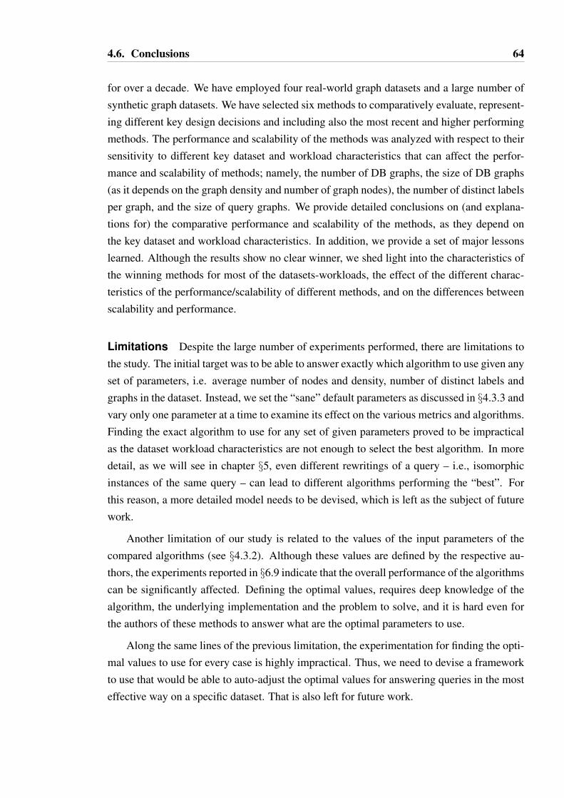
4.6. Conclusions 64
for over a decade. We have employed four real-world graph datasets and a large number ofsynthetic graph datasets. We have selected six methods to comparatively evaluate, represent-ing different key design decisions and including also the most recent and higher performingmethods. The performance and scalability of the methods was analyzed with respect to theirsensitivity to different key dataset and workload characteristics that can affect the perfor-mance and scalability of methods; namely, the number of DB graphs, the size of DB graphs(as it depends on the graph density and number of graph nodes), the number of distinct labelsper graph, and the size of query graphs. We provide detailed conclusions on (and explana-tions for) the comparative performance and scalability of the methods, as they depend onthe key dataset and workload characteristics. In addition, we provide a set of major lessonslearned. Although the results show no clear winner, we shed light into the characteristics ofthe winning methods for most of the datasets-workloads, the effect of the different charac-teristics of the performance/scalability of different methods, and on the differences betweenscalability and performance.
Limitations Despite the large number of experiments performed, there are limitations tothe study. The initial target was to be able to answer exactly which algorithm to use given anyset of parameters, i.e. average number of nodes and density, number of distinct labels andgraphs in the dataset. Instead, we set the “sane” default parameters as discussed in §4.3.3 andvary only one parameter at a time to examine its effect on the various metrics and algorithms.Finding the exact algorithm to use for any set of given parameters proved to be impracticalas the dataset workload characteristics are not enough to select the best algorithm. In moredetail, as we will see in chapter §5, even different rewritings of a query – i.e., isomorphicinstances of the same query – can lead to different algorithms performing the “best”. Forthis reason, a more detailed model needs to be devised, which is left as the subject of futurework.
Another limitation of our study is related to the values of the input parameters of thecompared algorithms (see §4.3.2). Although these values are defined by the respective au-thors, the experiments reported in §6.9 indicate that the overall performance of the algorithmscan be significantly affected. Defining the optimal values, requires deep knowledge of thealgorithm, the underlying implementation and the problem to solve, and it is hard even forthe authors of these methods to answer what are the optimal parameters to use.
Along the same lines of the previous limitation, the experimentation for finding the opti-mal values to use for every case is highly impractical. Thus, we need to devise a frameworkto use that would be able to auto-adjust the optimal values for answering queries in the mosteffective way on a specific dataset. That is also left for future work.

65
Chapter 5
Subgraph Querying with Parallel Use ofQuery Rewritings and Alternative Algo-rithms
[ X \
Despite the large attention the problem of subgraph query processing has enjoyed withinthe data management/mining communities and the large number of methods that have beendeveloped, scalability and efficiency remain an elusive goal, owing to the NP-Complete na-ture of the underlying subgraph isomorphism test. We analyze this problem and present keynovel discoveries and observations on the nature of the problem which hold across querysizes, datasets, and top-performing algorithms. Firstly, we show that algorithms (for boththe decision and matching versions of the problem) suffer from straggler queries, whichdominate query workload times. If one were to cap query times and not to report resultsfor queries exceeding the cap (personal communication with authors of [11], 2015), this canlead to erroneous conclusions of the methods’ relative performance. Secondly, we study andshow the dramatic effect that isomorphic graph queries can have on query times. Thirdly,we show that for each query, isomorphic queries based on proposed query rewritings canintroduce large performance benefits. Fourthly, we observe that straggler queries are largelyalgorithm-specific: many challenging queries to one algorithm can be executed efficiently byanother. Finally, the above discoveries naturally lead to the derivation of a novel frameworkfor subgraph query processing, resting on query graph rewritings (producing graphs that areisomorphic to the original query) and on using multiple alternative algorithms. The centralidea is to employ parallelism in a novel way, instead of trying to parallelize the subgraphisomorphism algorithm, whereby parallel matching/decision attempts are initiated, each us-

5.1. Introduction 66
ing a query rewriting and/or an alternate algorithm. Such an approach is common to otherNP-hard problems, where parallelizing the underlying algorithm is not easily feasible andthus running parallel instances of the same or alternative algorithms is a better approach,known as portfolios of algorithms. The framework is shown to be highly beneficial acrossalgorithms and datasets.
5.1 Introduction
With our work, we explore the strengths and weaknesses of existing FTV and SI methodsfor all versions of the subgraph querying problem, and we exploit the strong points of everyalgorithm by combining them in parallel executions to achieve large performance gains in thesubgraph querying problem. Our analysis aims to (i) lead to interesting novel findings aboutthe nature of the problem and existing solutions, (ii) analyze and quantify said discoveriesand their effect on well-established existing solutions, and (iii) show that the findings can beused to develop a framework that can offer large performance gains. Specifically, we first rec-ognize the existence of “straggler” queries; i.e., queries whose execution time is dramaticallyhigher than the rest. This holds for all query workloads and all datasets examined and acrossall tested FTV and SI algorithms. Subsequently, we reveal and quantify the interesting factthat isomorphic instances of queries can have a wild variation in querying times. Then wegenerate isomorphic instances of the original query using statistics on vertex-label frequen-cies and/or vertex degrees and we investigate their performance. Moreover, for SI methods inparticular, we additionally show that challenging queries are algorithm-specific, with a strag-gler query for one algorithm possibly being easy for others. Finally, we incorporate thesefindings in a novel framework, coined the Ψ-framework, that exploits parallelism for bothFTV and SI methods, achieving large performance gains. Specifically, instead of trying tocome up with new algorithms for sub-iso testing, we utilize isomorphic query rewritings andexisting alternative algorithms in parallel. Extensive experimentation shows that our frame-work can be highly beneficial across both real and synthetic datasets and query workloads,and for both FTV and SI methods.
5.2 Related Work and Contributions
The numerous proposed FTV and SI methods have been extensively discussed in §2.3.The target of the current chapter is to propose empirical ways in order to expedite the sub-graph queries, originated from the strengths and weaknesses of all proposed methods. Wemainly focus on the various SI methods and thus, we leave intact the indexing and filteringstage of the used FTV methods.

5.3. Experimental Setup 67
As subgraph querying is an important problem, we expect that many researchers willkeep focusing on trying to improve upon existing algorithms in the future. Indeed, sincethe publication just a few years ago of iGraph-v2[8], comprehensively comparing the thenstate of art SI algorithms, newer algorithms have been proposed, e.g. [55], with better per-formance. Nonetheless all algorithms show exponential execution times even at small querysizes (up to 10 edges) (BoostIso[56]). Our contributions aim to help this process in twoways. First, by revealing key insights, based on comprehensive experimentation, about theproblem itself and how they affect well-known algorithms. Second, by shedding light onto anovel overall approach to the problem and its benefits. Namely, instead of focusing solely ondeveloping new solutions by improving earlier algorithms, try to benefit from the wealth ofideas already existing within previous algorithms! Specifically, our findings show that dif-ferent algorithms are appropriate for different queries. Furthermore, they show that differentquery rewritings are appropriate for different queries and for different algorithms! Finally,the existence of straggler queries poses new challenges for the performance comparison ofdifferent algorithms, needing more detailed performance metrics and experimenting withmore challenging queries. All current works miss the above points: (i) they only considerone query rewriting, if at all, for all queries, (ii) they use only one algorithm for all work-load queries, and (iii) they do not stress-test their algorithms with more challenging queries(e.g., larger sizes). Our framework shows that such misses also lead to misses of dramaticperformance improvements.
5.3 Experimental Setup
5.3.1 Algorithms
For the FTV methods, we chose Grapes[11] and GGSX[12] to be included in our exper-iments, accredited as top-performing based on our experiments in chapter §4.
For the SI methods, we opted for methods (i) whose code is publicly available or madeavailable to us by the authors upon request, so any conclusions would not be implementationdependent, (ii) that were well recognized as well performing and (iii) used by many papersfor comparison purposes. We selected QuickSI[35], GraphQL[24], sPath[29], TurboIso[55],and Boosted-TurboIso[56]. With respect to CFL-Match [57], its authors did not respond toour request for their code, and thus CFL-Match is not included in our experiments.
A more detailed description of the in-use algorithms can be found in §3.1.

5.3. Experimental Setup 68
5.3.2 Setup
Experiments with Grapes and GGSX were conducted on a small cluster consisting of 5nodes, each featuring an Intel Core i5-3570 CPU (3.4GHz, 4 physical cores, 6MB cache),16GB of RAM, 500GB disk per node, and running Ubuntu Linux 14.04. Experiments withQuickSI, GraphQL, sPath, TurboIso and BTI (i.e., the SI methods) were conducted on a Win-dows 7 SP1 host, with 2 Intel Xeon E5-2660 CPUs (2.20GHz, 20MB cache) with 8 cores/16vcores per CPU, 128GB of RAM, and 3.5TB disk. With the term “experiment”, we refer tothe subgraph matching process of 1 query graph against 1 stored graph. For practical pur-poses, we allowed a maximum limit of 10 mins for each query to be processed. Beyond thattime, the execution is terminated and we proceed with the next query in the workload. Pleasenote that this 10’ limit does not apply in the indexing phase of the individual algorithms.
For Grapes and GGSX we used the implementations provided by their respective au-thors. However, in the case of Grapes, we had to alter the source code so that the VF2verification step returns after the first match of the query graph, as opposed to the originalimplementation which was returning all possible matches. The reason for this is that FTVmethods are mainly designed to retrieve the graphs that contain the query as an answer. ForQuickSI, GraphQL and sPath, we used the implementation provided by [8]. For TurboIso,we obtained the binary code from the authors and for BTI we obtained the source code fromGitHub1 where it was publicly available.
We used the default values for the input parameters of the compared algorithms, asthey were defined by their respective authors in the relevant publications and/or in theirimplementation code. More specifically:
• For GGSX and Grapes, we enumerated paths of up to size of 4.• We ran Grapes with 1 and 4 threads; results for executions with 1 (respectively 4)
threads are denoted by Grapes/1 or GR/1 (respectively Grapes/4 or GR/4).• For GraphQL, we used a refined level of iterations of pseudo-subgraph isomorphismr = 4.• For sPath, we used a neighborhood radius of 4 and maximum path length 4.• TurboIso does not require any input parameter. However, by default only queries up
to 25 vertices are able to execute. We were not able to change this option because ofthe binary that was made available to us.• BTI, too, does not require any input parameter. However, compared to the rest of the
in-use SI methods, BTI only allows one label per vertex on the stored graph. Thus, wewere not able to execute experiments with some of our datasets (see §5.3.3).• For all SI methods the number of searched embeddings of the pattern graph on the
stored graph is capped at 1000; i.e., after finding the first 1000 matches, the algorithms1 https://github.com/UltraHector/BoostIsoGraphAdaptation

5.3. Experimental Setup 69
terminate. We note that for GraphQL, sPath, QuickSI and BTI the number of embed-dings is configurable, but for TurboIso it is hardcoded (an option we cannot changebecause of the binary made availabe to us).
A detailed description of the employed algorithms can be found in §3.1.
5.3.3 Datasets
We chose datasets which (a) have also been used by other studies, so as to enable possibledirect comparisons, and (b) have key characteristics covering a large part of the design space(e.g., regarding graph size and density).
For the FTV methods, we have used PPI and the Synthetic datasets and their charac-teristics can be seen in Table 3.1. PPI (used in [11, 9]) is a real dataset representing 20different protein-protein interaction networks, as discussed in §3.2.2. The majority of ex-isting real datasets that were used for the FTV methods comprises of relatively small andsparse graphs. In [9] we showed that, for such datasets, both Grapes and GGSX performadequately well. For our current study we are further interested in more challenging datasetsand we thus employ the additional synthetic dataset generated with GraphGen[60], allow-ing various parameters of interest to be specified; namely, number of graphs and numberof labels in the dataset, average number of nodes and density per graph). A more detaileddescription of how GraphGen constructs the dataset can be found in §3.2.1.
Datasets used for the SI methods consist of only one graph, as the primary task of thesemethods is to find all occurrences of the pattern graph in the large stored graph. Table 3.2summarizes the characteristics of the three real datasets – namely yeast, human and wordnet– that we have used for the SI methods. Yeast and human were previously used in [8], whilewordnet2 was used in [23]. Finally, yeast and human, unlike wordnet, allow multiple labelson each node, and thus we were able to execute BTI only on wordnet, as discussed in §5.3.2.
5.3.4 Query Workloads
To generate each of the query graphs, we follow the procedure described in §3.2.3.
For the FTV methods, for the synthetic dataset, we used queries of size 24, 32 and40 edges for Grapes/1 and Grapes/4. We did not run GGSX against the synthetic dataset,because of excessive amount of time required for the experiments to complete. For the PPIdataset, we used queries of size 16, 20, 24, and 32 edges.
For the SI methods, we used 200 queries of 10, 16, 20, 24 and 32 edges. For QuickSIwe only report results against the yeast dataset, as (i) it was the easiest dataset used for
2http://vlado.fmf.uni-lj.si/pub/networks/data/dic/Wordnet/Wordnet.htm

5.3. Experimental Setup 70
the SI methods to process (smallest number of nodes with highest number of distinct labelscompared to human and yeast as discussed in §3.2.2), and (ii) QuickSI always had manymore cases, compared to GraphQL and sPath, where query processing exceeded the 10’ cap(figures 5.4). Because of implementation restrictions with TurboIso and the binary that wasmade available to us, we were not able to execute queries with more than 25 vertices, andas a result, from the 200 constructed queries of 32-edges workload, none of them qualifyfor yeast and only 60 of them qualify for human dataset that we include on our experiments.BTI does not support the use of multiple labels per node. Thus, we do not present any resultswith BTI against the yeast and human dataset. Finally, to restrict the number of executedexperiments, we opted to execute BTI instead of TurboIso as the third alternative algorithmin wordnet.
For all used methods, the majority of the queries completed in under 2”. We call themeasy queries. Another portion of queries had processing times in the 2” to 600” range; wedenote these 2”-600” queries. We use the term completed to refer to all queries that finishedwithin the 10’ limit; those that did not are called hard or killed.
5.3.5 Performance Metrics
For every query against a stored graph, we measure the Execution Time, denoted exec
time, for both FTV and SI methods, while avg exec time denotes the average execution time.Specifically for this specific chapter, for FTV methods, this is the pure subgraph isomor-phism time; i.e., excluding the index loading and filtering times, which add only a trivialoverhead, unless stated otherwise. For FTV methods reported times are in seconds, whilefor SI methods times are in milliseconds, unless stated otherwise.
Let qi be a given query and tMi the exec time of qi over method M . Let also qi,j be thej-th isomorphic instance of qi and tMi,j the exec time of qi,j over method M . Finally, let tΨi,jbe the exec time of qi,j over our proposed Ψ-framework, and tGR−M
i be the execution timeof qi over the hybrid combination of Grapes (GR) with method M over all the graphs in thedataset.
We define the (max/min) metric as:maxj(tMi,j)
minj(tMi,j). The minimum value of this metric is 1,
indicating that there are no variations between the min and max exec time. The higher thevalue of this metric, the higher the differences between the min and max exec time achievedby the isomorphic query instances.
We also define the speedup∗ metric as: tMiT
, where T is set to: (i) minj(tMi,j), when
comparing against the various isomorphic instances of qi, (ii) minM(tMi,j), when comparingagainst different methods, and (iii) tΨi , when comparing against our Ψ-framework. speedup∗
represents what we lose in performance if we choose the original method over the various

5.4. Straggler Queries 71
alternatives; i.e., speedup∗ equals the maximum attainable speedup over the original method,if we chose the best of the examined alternatives. For comparison purposes, for queries thatwere killed at the 10’ limit we use this time (i.e., 600”) as their minimum execution time.
Finally, both (max/min) and speedup∗ metric have their QLA and WLA version, as wediscussed in §3.3.4, denoted with a matching subscript; e.g. speedup∗QLA.
5.4 Straggler Queries
We know that as the dataset grows in terms of the size of graphs (i.e. density, number ofnodes), query processing becomes harder; likewise, query processing becomes harder as thequery graph incresases, as discussed in [9] and in chapter §4. But are these statements truefor all queries-dataset stored graph combinations? Running many queries against the wholedataset can hide the details of how much time is required per individual graph-query pair. Inthe case that a small portion of such pairs dominates the whole execution time, then by justlooking at the whole query workload execution times it is easy to draw wrong conclusionsabout the algorithms’ performance. Also, several related works choose to ignore querieswhose execution is much higher compared to the rest. To investigate the above, in this studywe execute each individual query against a single stored graph at a time, for both FTV andSI methods.
Observation 1: In all workloads generated by us or found in other papers, our experimentsshow “stragglers”; i.e., queries whose processing time is many orders of magnitude highercompared to the rest.
To support our observation, we present the results from our experiments on the afore-mentioned datasets against both FTV (figures 5.1 and 5.2) and SI methods (figures 5.3 and5.4).
FTV methods
Figures 5.1 and 5.2 present the results from the query workloads on the FTV methods.Specifically, figures 5.1(a) and 5.1(b) show the average execution times for the correspond-ing algorithms for the synthetic and the PPI dataset accordingly (GGSX/synthetic resultsare omitted; see §5.3.2). Figure 5.2 presents the percentage of the sub-iso tests that wereeasy, 2”-600”, and hard for both the synthetic and PPI datasets. As expected, Grapes/4 hasa much smaller percentage of killed queries compared to Grapes/1 and GGSX. A notablething here is that, the average execution time of easy queries is measured to some tens of

5.4. Straggler Queries 72
0.01
0.1
1
10
100
GR/1 GR/4
WL
A-A
vg
ex
ec t
ime
(s)
easy 2’’-600’’ completed
(a) Synthetic dataset, WLA-Average exec time (s)
0.01
0.1
1
10
100
GR/1 GR/4 GGSX
WL
A-A
vg
ex
ec t
ime
(s)
easy 2’’-600’’ completed
(b) PPI dataset, WLA-Average exec time (s)
Figure 5.1: WLA-Average exec time (s) in FTV methods
milliseconds and the average execution time of 2”-600” is hundreds of seconds, which re-sults in an average execution time of completed queries measured in tens of seconds. Inother words, although for both Grapes/1 and Grapes/4 the percentage of 2”-600” queries isonly < 5% in the synthetic dataset and < 10% in PPI, the average execution time across allcompleted queries is significantly affected; that is, the most expensive queries dominate theoverall execution time.
SI methods
Figures 5.3 and 5.4 present the results from the query workloads on the SI methods(QuickSI-[human/wordnet], TurboIso-wordnet and BTI-[human/yeast] results are omitted;see §5.3.2), while tables 5.1 and 5.2 give the average execution times and percentages for

5.4. Straggler Queries 73
0
20
40
60
80
100
GR/1 GR/4 GR/1 GR/4 GGSX
% o
f q
uer
ies
easy 2’’-600’’ hard
PPIsynthetic
Figure 5.2: Percentages of easy, 2”-600”, and hard queries in FTV methods
GraphQL sPath QuickSI TurboIso
10-e
dgeq
AET easy (ms) 66.84 134.78 131.67 92.69% of easy 100 99.5 99 99.5
AET 2”-600” (ms) - 2871.44 50367.40 -% of 2”-600” 0 0.5 1 0
% of hard 0 0 0 0.5
32-e
dgeq
AET easy (ms) 130.66 120.71 96.62 -% of easy 80 91 67.5 -
AET 2”-600” (ms) 140812 140781 78917.2 -% of 2”-600” 6.5 3 6 -
% of hard 13.5 6 26.5 -
Table 5.1: Results for SI methods on the yeast dataset (AET: Average exec time)
GraphQL sPath TurboIso
10-e
dgeq
AET easy (ms) 179.49 209.91 87.04% of easy 100 98 100
AET 2”-600” (ms) - 182392 -% of 2”-600” 0 1 0
% of hard 0 0 0
32-e
dgeq
AET easy (ms) 246.31 277.13 173.35% of easy 71.5 84.5 73.33
AET 2”-600” (ms) 93523.7 31817 148.695% of 2”-600” 4.5 4.5 8.33
% of hard 24 11 18.33
Table 5.2: Results for SI methods on the human dataset (AET: Average exec time)
10- and 32-edge easy, 2”-600” and hard queries for the yeast and human datasets. We usethe 10-edge query results to compare our findings with those presented in iGraph-v2[8] andfor the common algorithms, i.e., GraphQL, sPath and QuickSI. iGraph-v2 used small query

5.4. Straggler Queries 74
1
10
100
1000
10000
100000
1x10⁶
GQL SP QSI TI
WL
A-A
vg
ex
ec t
ime
(ms)
easy 2’’-600’’ completed
yeast
(a) yeast dataset, WLA-Average exec time (ms)
1
10
100
1000
10000
100000
1x10⁶
GQL SP TI
WL
A-A
vg
ex
ec t
ime
(ms)
easy 2’’-600’’ completed
human
(b) human dataset, WLA-Average exec time (ms)
1
10
100
1000
10000
100000
GQL SP BTI
WL
A-A
vg
ex
ec t
ime
(ms)
easy 2’’-600’’ completed
(c) wordnet dataset, WLA-Average exec time (ms)
Figure 5.3: WLA-Average exec time (s) in SI methods

5.4. Straggler Queries 75
0
20
40
60
80
100
GQL SP QSI TI GQL SP TI GQL SP BTI
% o
f q
uer
ies
easy 2’’-600’’ hard
wordnethumanyeast
Figure 5.4: Percentages of easy, 2”-600”, and hard queries in SI methods
sizes (up to 10 edges) and showed that the best performing algorithm is GraphQL, because itmanaged to complete all tested query workloads. With our experiments, we confirm this forboth yeast and human datasets and for queries of size 10 edges. GraphQL performs the bestamong the three, having also 0% of hard queries. However, the picture is totally reversedwhen looking at the rest of the queries.
Specifically, regarding table 5.1 and the yeast dataset, for 10-edge queries, results forsPath and QuickSI are comparable, with GraphQL having 0% of hard queries, whereas Tur-boIso is already lagging behind with 0.5% of hard queries. The same is valid for the easy
queries of 32 edges. However, the picture is totally reversed when looking at the rest of thequeries. In this case, the percentage of killed queries is double for GraphQL and quadruplefor QuickSI compared to sPath.
Additionally, regarding table 5.2 and the human dataset, where QuickSI is replaced withTurboIso (§5.3.2), GraphQL and TurboIso perform better compared to sPath that already hasa 1% 10-edge query that takes 2”-600” to execute. The picture is again reversed for all threecompeting algorithms as sPath proves to be the most robust at 32-edge queries, with only11% of hard queries.
Because of implementation restrictions, we were not able to execute queries of >25vertices with TurboIso (see §5.3.2); thus no queries of 32 edges were executed for yeastand only 60 queries of 32 edges qualified for human. As a result, the presented results forTurboIso on human and yeast are not directly comparable with the numbers provided forGraphQL and sPath. However, we note that for the same 60 32-edge queries executed overhuman dataset on all 3 algorithms, TurboIso encountered more hard queries than the othertwo contestants. Finally, although BTI is the latest proposed method, it suffers from morehard queries compared to GraphQL and sPath for the wordnet dataset.

5.5. Isomorphic queries 76
GraphQL and sPath are the 2 alogrithms executed against all 3 datasets (figures 5.3and 5.4, tables 5.1 and 5.2). Based on our experiments, sPath performs overall better thanGraphQL having (i) smaller average execution times on the completed queries and (ii) smallerpercentages of hard queries in yeast and human datasets. However, in wordnet this behavioris reversed. Thus, it’s very difficult to claim that one algorithm is performing better thanthe other. In fact, in order to claim that, we need to define a performance metric of interest.Such a performance metric could be the percentage of killed queries, but that still dependson the time limit imposed on query processing. For example, in wordnet, if the thresholdwas 2”, then sPath would be better than GraphQL, but if we change this threshold the picturechanges.
We summarize our results to the following 3 conclusions: (1) Some queries are hard.(2) Different algorithms have different percentages of completed queries; thus, different al-gorithms find different queries hard. (3) As the most expensive queries dominate the averageexecution time, one must include a sufficient number of hard queries in order to draw con-clusions about the relative performance of the algorithms.
5.5 Isomorphic queries
Various proposed SI methods ([24, 29, 35]), as well as iGraph-v2[8] that compares them,observe that the search order on the query can have a huge impact on query processingtime. We agree with this claim. This behavior is typical on other NP-hard problems, asdiscussed in §2.7 ([116]). In the current study, we take a further step and instead of relyingon the order that the individual method imposes, we generate our own isomorphic queryrewritings. To achieve this, we maintain the structure of the query graph and the labels onthe nodes unchanged, and we permute the node IDs. Subsequently, we transform the querygraph to an input format compatible with each individual method and we perform the queryprocessing. The same effect of constructing isomorphic query graphs to the original querygraph can be achieved by permuting rows/columns of the original graph in an adjacencymatrix representation. In the following experiments, we use a total of 6 different rewritingsper query, leading to the following observation.
Observation 2: Queries which are isomorphic to the original query graph can have widelyand wildly different execution times.
We attribute this behavior to the fact that all proposed methods do not define an abso-lutely strict order in which the nodes of the query are matched, as it would be too compu-tationally expensive to compute a globally optimal join plan. Thus, all proposed methods,

5.5. Isomorphic queries 77
similarly to other NP-hard problems [116], rely on heuristics (see §5.3.1) in order to min-imize the search space for the join plan. However, given the fact that SI methods definea more strict order in which the nodes of the query are matched, this wide execution timevariation (as we will see later on in this chapter) was not initially expected.
1
10
100
1000
10000
100000
1x10⁶
(max
/min
) QL
A
GR/1GR/4
GGSX
PPIsynthetic
Figure 5.5: Average (max/min)QLA for FTV methods
Grapes/1 Grapes/4 GGSX
synt
hetic
stdDev 86,700.40 65,988.40 -min 1.06 1.02 -max 3,820,000.00 3,490,000.00 -
median 3.90 4.45 -
PPI
stdDev 469,934 395,285 1,020,000min 1.03 1.02 1.01max 3,680,000 3,160,000 12,000,000
median 1,186.51 11.19 109,086.00
Table 5.3: (max/min)QLA statistics for FTV methods
FTV methods
Figure 5.5 depicts the QLA average value of the (max/min) metric for the syntheticand PPI datasets, for the FTV methods (GGSX results are omitted for the synthetic dataset;see §5.3.4), whereas figure 5.6 presents the (max/min)QLA for different query sizes onthe PPI dataset. Table 5.3 additionally reports the stdDev, min, max and median values of(max/min)QLA. In the calculations, we did not include a small number of queries thatwere not helped by any of the isomorphic instances tried; i.e., queries that were hard onall tested isomorphic instances of the query. This behavior occurred in 0.0036% and 1.4%of queries for Grapes/1 on the synthetic and PPI datasets respectively, in 0.37% of queries
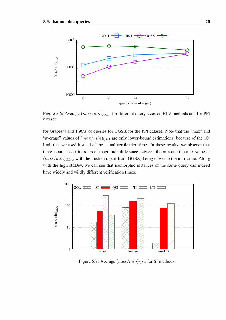
5.5. Isomorphic queries 78
10000
100000
1x10⁶
16 20 24 32
(max
/min
) QL
A
query size (# of edges)
GR/1 GR/4 GGSX
Figure 5.6: Average (max/min)QLA for different query sizes on FTV methods and for PPIdataset
for Grapes/4 and 1.96% of queries for GGSX for the PPI dataset. Note that the “max” and“average” values of (max/min)QLA are only lower-bound estimations, because of the 10’limit that we used instead of the actual verification time. In these results, we observe thatthere is an at least 6 orders of magnitude difference between the min and the max value of(max/min)QLA, with the median (apart from GGSX) being closer to the min value. Alongwith the high stdDev, we can see that isomorphic instances of the same query can indeedhave widely and wildly different verification times.
1
10
100
1000
(max
/min
) QL
A
GQL SP QSI TI BTI
wordnethumanyeast
Figure 5.7: Average (max/min)QLA for SI methods

5.5. Isomorphic queries 79
GraphQL sPath QuickSI TurboIso BTI
yeas
t
stdDev 287.5 533.8 1685.7 704.7 -min 1.0 1.0 1.0 1.0 -max 7286.3 6695.8 15021.6 14053.4 -
median 1.4 1.3 1.6 2.1 -
hum
anstdDev 440.1 662.7 - 1214.7 -
min 1.0 1.0 - 1.0 -max 4115.0 4087.8 - 9030.0 -
median 1.8 1.9 - 1.9 -
wor
dnet
stdDev 20.5 396.8 - - 1635.1min 1.0 1.0 - - 1.0max 646.4 3081.1 - - 31121.8
median 1.2 1.3 - - 1.1
Table 5.4: (max/min)QLA statistics for SI methods
1
10
100
1000
10000
10 16 20 24 32
(max
/min
) QL
A
query size (# of edges)
GQL SP TI
Figure 5.8: Average (max/min)QLA for different query sizes on SI methods and for humandataset
SI methods
Figure 5.7 reports the QLA-average values of the (max/min) metric for the yeast, hu-man and wordnet datasets, for the tested SI methods (QuickSI-[human/wordnet], TurboIso-wordnet and BTI-[human/yeast] results are omitted; see §5.3.4). Additionally, figure 5.8presents the (max/min)QLA for different query sizes on the PPI dataset. Table 5.4 reportsthe stdDev, min, max and median value of (max/min)QLA. We report that 4.2%, 8.2% and1.5% of queries were not helped by any tested isomorphic query instances for GraphQL andfor yeast, human and wordnet respectively. For sPath the corresponding values are 2.1%,1.4% and 11.8%, and for QuickSI 8.6% of the queries were not helped for the yeast dataset.For TurboIso 0.88% and 4.19% of the queries were not helped for yeast and human respec-tively and for BTI and wordnet the corresponding value is 7.7%.

5.6. Graph query rewriting 80
The QLA-average (max/min) for the SI methods is up to 3 orders of magnitude lowerthan that of the FTV methods. This is somewhat expected as the SI methods define a morestrict order in which the nodes of the query are matched and thus leave less space for wildvariations. However, this order is still significantly affected by the initial node ids of thequery, and thus we still see per-query (max/min) values of up to 2 orders of magnitude.
We summarize our overall results to the following conclusions: (1) For every isomorphictest to be executed, given a query graph q and a stored graph, there is an isomorphic versionof q that can take anywhere from 2 to 6 orders of magnitude more time to execute comparedto the least expensive version of the query. This holds across all algorithms and datasetstested. This is a typical behavior of other algorithms proposed for NP-hard problems, asdiscussed in §2.7. Specifically, we have seen that these algorithms also employ differentheuristics and their performance is significantly affected by the search order they impose.(2) The harder the queries (higher query sizes), the higher these number are, as it can be seenby figures 5.6 and 5.8.
5.6 Graph query rewriting
Having established that isomorphic versions of a query can have dramatically differentexecution times, we set out to construct our own specific rewritings, constructing graphs iso-morphic to the original queries, with the aim to capture these benefits. We have developedand experimented with several such query rewritings. We outline below five such rewrit-ings, all performed by carefully permuting the node IDs in the query graph: The discussionassumes a query graph and a stored graph.
• Query Rewriting ILF (Increasing Label Frequency):In a preprocessing step, we compute the frequencies of all node labels in the storedgraph, sorted in increasing frequency order. Given this order, we produce a rewritingof the query graph so if i, j are the node IDs of query graph nodes ni, nj , L(ni), L(nj)
are their labels, and f(L(·)) is the frequency of a label L(·) in the stored graph, thenf(L(ni)) < f(L(nj)) ⇒ i < j. Ties can appear in 2 cases: (i) two or more querynodes have the same label, or (ii) two or more query nodes have different labels butwith the same frequency. These ties are broken arbitrarily.• Query Rewriting IND (Increasing Node Degree):
The nodes of the query are sorted in increasing node degree order; i.e., if ni, nj are twoquery graph nodes, and d(·) is the degree (number of edges) of a node, then d(ni) <
d(nj) ⇒ i < j. In the case of nodes with the same number of edges, ties are brokenarbitrarily.

5.6. Graph query rewriting 81
• Query Rewriting DND (Decreasing Node Degree):This rewriting is similar to the IND rewriting but the nodes of the query are sorted indecreasing node degree and the node ids are assigned accordingly.• Query Rewriting ILF+IND:
This rewriting is the same as ILF above, with ties being broken in an IND manner: i.e.,nodes with smaller outgoing degree get a lower node id.• Query Rewriting ILF+DND:
This rewriting is the same as ILF+IND, with ties being broken in a DND manner.
In order to conduct our experiments, and to perform our query rewriting, based on theinitial query node IDs of the original query, we break ties by respecting the order of nodes onthe original queries. In other words, let ni and nj be two query graph nodes with node IDsi < j, that belong in the same tie group; i.e. they have the same label or the same degree,or both the same label and degree. Then, in the rewritten query the node IDs will be i′ < j′.Undoubtedly, this is not the only way to resolve ties; for example we could randomly assignnode IDs on the nodes that belong in the same tie group. Additionally, although our currenttie-breaking approach is deterministic, it is still based on the initial assignment of IDs tonodes, which is in turn arbitrary and random in its own right, e.g., any random rewritingcould have been the original form of the query graph.
In §3.1.2 and §5.5, we discussed how the various methods decide the optimal join planso as to match the query vertices to the vertices on the stored graph. However, we have seenthat in some cases ties (symmetries) still exist, in other cases that not all possible join plansare considered. For example, QuickSI tries to resolve symmetries by making the constructedMST denser, whereas GraphQL considers only left-deep join plans to define a good searchorder. However, ties still exist and it is expected that these ties are resolved by the variousalgorithms by looking at the query node IDs. Thus, intuitively, and in case of ties, given thatnode ID i < j, it is expected that ni will be matched earlier than node nj . Time-wise, thismight have a tremendous effect on the algorithm’s performance depending on the number ofthe actual join operations to consider.
Figure 5.9 presents an example of the above rewritings. Note that the ILF+IND rewritingin 5.9(d) is another valid isomorphic ILF rewriting. Ties are (utterly) broken in an arbitraryway, and thus one may compute several different isomorphic graphs for the same rewriting.
Indicatively3, in figures 5.10 and 5.11 we report the WLA average processing timesof the original query and the 5 proposed query rewritings for the PPI and yeast datasets,as well as the corresponding percentages of the hard queries. For the FTV methods, thebest performing rewritings are ILF and ILF+DND, with the percentage of hard queries be-
3We obtained similar results for the synthetic dataset for the FTV methods and the human and wordnetdatasets for all used SI methods. The sole exception was sPath, whose percentage of hard queries increasedslightly for the wordnet dataset.

5.6. Graph query rewriting 82
A A
AB
B
C
C0
123
45
6
(a) Original
A A
AB
B
C
C0
1
2
34
56
(b) ILF
A A
AB
B
C
C
0
1
2
3 4
5
6
(c) IND
A A
AB
B
C
C0
12
3
4
5
6
(d) ILF+IND
Figure 5.9: Isomorphic queries generated with different rewritings (assuming the label fre-quencies in the stored graph are: “A”=20, “B”=15, “C”=10)
0
50
100
150
200
250
300
GR/1 GR/4 GGSX
WL
A-A
vg
ex
ec t
ime
(s)
OrigILF
INDDND
ILF+INDILF+DND
(a) WLA-Average exec time (s)
0
5
10
15
20
25
30
35
40
45
GR/1 GR/4 GGSX
% o
f h
ard
qu
erie
s
OrigILF
INDDND
ILF+INDILF+DND
(b) percentage of hard queries
Figure 5.10: Results for individual query rewritings for FTV on PPI dataset

5.6. Graph query rewriting 83
0
10000
20000
30000
40000
50000
60000
70000
80000
GQL SP QSI TI
WL
A-A
vg
ex
ec t
ime
(ms)
OrigILF
INDDND
ILF+INDILF+DND
(a) WLA-Average exec time (ms)
0
2
4
6
8
10
12
GQL SP QSI TI
% o
f h
ard
qu
erie
s
OrigILF
INDDND
ILF+INDILF+DND
(b) percentage of hard queries
Figure 5.11: Results for individual query rewritings for SI methods on yeast dataset
ing significantly improved. For the SI methods, the picture is slightly different. GraphQLshows no considerable improvement for each rewriting individually; as a matter of fact, thereare rewritings leading to higher average execution times than the original query does. ForsPath, the DND and ILF+DND rewritings reduce the percentage of killed queries from 2.8%to 2.4%. For QuickSI, ILF+DND reduced the percentage of killed queries from 11.3% to10.2%, but DND only brings it down to 10.9%. For TurboIso, IND and ILF+IND reduce thepercentage of killed queries from 1% to 0.875%. Note that in the case of TurboIso, results arenot directly comparable with the rest of the contestants because no queries of 32 edges areincluded (see §5.3.4). More importantly, note that there is no single rewriting that managesto improve all algorithms across all datasets and workloads. However, if we were to executein parallel various isomorphic rewritings, we would achieve large performance gains.

5.6. Graph query rewriting 84
Observation 4: “Stragglers” can have isomorphic counterparts which are not stragglers.Table 5.5 quantifies the percent reduction of straggler queries for both FTV and SI methodswhen using isomorphic query counterparts for the tested datasets.
GR/1 GR/4 GGSX GQL SP QSI TI BTI
FTV synthetic 98.8% 100% - - - - - -
PPI 91.1% 94.1% 94.7% - - - - -
SI
yeast - - - 2.32% 25% 23.9% 12% -human - - - 15.5% 68.2% - 24.9% -human - - - 6.3% 9.2% - - 36.9%
Table 5.5: Percent reduction of straggler queries for FTV and SI methods using isomorphicquery counterparts
Figures 5.12 and 5.14 present the achieved speedup∗ of such an execution. Similarly, asin §5.5, the max and average reported speedup∗ represent a lower-bound estimation becauseof the value 10’ that we use for the hard queries that were killed. Additionally, in ourcalculations we do not include the few queries that were killed in both the original instanceand in all the rewritings of the query (see §5.5).
1
10
100
1000
10000
100000
1x10⁶
spee
du
p*
QL
A
GR/1GR/4
GGSX
PPIsynthetic
Figure 5.12: Average speedup∗QLA for FTV methods across rewritings
FTV methods
Figure 5.12 presents the average speedup∗QLA for the FTV methods for the synthetic andPPI datasets (GGSX/ synthetic results are omitted; see §5.3.4). Additionally, table 5.6 reportsthe QLA stdDev, min, max and median of speedup∗QLA. Moreover, as we increased the sizeof the queries, speedup∗QLA increased by up to 5 orders of magnitude, as it can be seen byfigure 5.13. Regarding the presented results in table 5.6, median speedup∗QLA is close to

5.6. Graph query rewriting 85
Grapes/1 Grapes/4 GGSX
synt
hetic
stdDev 53,785.70 24,267.60 -min 1.00 1.00 -max 3,820,000 2,110,000 -
median 1.36 1.24 -
PPI
stdDev 302,250 237,573 758,668min 1.00 1.00 1.00max 3,370,000 2,910,000 9,390,000
median 3.71 1.67 1,751.22
Table 5.6: speedup∗QLA statistics for FTV methods across rewritings
1
10
100
1000
10000
100000
1x10⁶
16 20 24 32
spee
du
p*
QL
A
query size (# of edges)
GR/1 GR/4 GGSX
(a) PPI dataset
1
10
100
1000
10000
100000
24 32 40
spee
du
p*
QL
A
query size (# of edges)
GR/1 GR/4
(b) Synthetic dataset
Figure 5.13: Average speedup∗QLA for different query sizes on FTV methods
min speedup∗QLA, evidencing again a wide variation in the benefits of the isomorphic queryrewritings. Keeping in mind that the majority of the queries are easy (figure 5.2), we come

5.6. Graph query rewriting 86
to the conclusion that large performance gains can come from improving the hard queries.Finally, the percentages of the queries that were not helped by any of the rewritings are thesame as presented in §5.5.
1
10
100
1000
spee
du
p*
QL
A
GQL SP QSI TI BTI
wordnethumanyeast
Figure 5.14: Average speedup∗QLA for SI methods across rewritings
GraphQL sPath QuickSI TurboIso BTI
yeas
t
stdDev 235.6 422.5 1193.0 498.7 -min 1.0 1.0 1.0 1.0 -max 7286.3 6695.8 15021.6 14053.3 -
median 1.1 1.1 1.3 1.7 -
hum
an
stdDev 259.9 492.4 - 695.1 -min 1.0 1.0 - 1.0 -max 4115.1 4087.8 - 8919.7 -
median 1.1 1.1 - 1.1 -
wor
dnet
stdDev 20.5 244.6 - - 1029.7min 1.0 1.0 - - 1.0max 646.4 3081.1 - - 31121.8
median 1.1 1.1 - - 1.0
Table 5.7: speedup∗QLA statistics for SI methods across rewritings
SI methods
Figure 5.14 presents the average speedup∗QLA for the SI methods for the yeast, humanand wordnet datasets (QuickSI-[human/wordnet], TurboIso-wordnet and BTI-[human/ yeast]results are omitted; see §5.3.4). Table 5.7 reports the stdDev, min, max and median ofthe speedup∗QLA. The percentages of the queries that were not helped by any rewritingare in accordance with those reported in §5.5. The performance of sPath could seeminglybe improved by one to two orders of magnitude across all datasets. The same holds for

5.7. Algorithm-specific Stragglers 87
QuickSI, TurboIso and BTI on the corresponding datasets. GraphQL could also be improvedby more than a factor of 10× on the yeast and human datasets. However, no significantimprovement was possible for GraphQL on wordnet. The reason why this is so, is somewhatsubtle. Apart from what the algorithms do internally to match the query, other culprits arethe characteristics of the actual stored graphs and the generated queries. Looking at thestatistics of the graphs (table 3.2), yeast and especially wordnet are very sparse graphs withsmall average node degree. Thus, the majority of the generated queries are paths, where therewritings based on node degrees are not effective in this case. Additionally for wordnet, thesmall number of labels (only 5) and the distribution of the frequencies of the labels beinghighly skewed leads to the generation of queries that in their majority contain only 1 or 2labels, with the second label appearing only once. As a result, the rewritings are of little usein these cases.
5.7 Algorithm-specific Stragglers
In §5.4, we notice that for the SI methods, different algorithms have different percent-ages of hard queries. With our experiments, we elaborated more on that and we found thatdifferent algorithms find different queries hard.
Observation 5: “Stragglers” are algorithm-specific; i.e., by evaluating the same queryworkloads with various algorithms, we have seen that a “straggler”-query for one algorithmcan be a typical query for some other algorithm.
GraphQL sPath QuickSI
yeas
t 2alg
stdDev 1094.57 1051.65 -min 1.00 1.00 -max 9189.36 9129.60 -
median 1.00 1.80 -
yeas
t 3alg
stdDev 1596.47 1255.34 2162.97min 1.00 1.00 1.00max 13060.10 12403.70 12312.70
median 1.00 1.88 1.32
hum
an
stdDev 1394.34 570.83 -min 1.00 1.00 -max 30873.80 4341.44 -
median 1.00 1.04 -
Table 5.8: speedup∗QLA statistics when utilizing different algorithms on SI methods for yeastand human
Here, we present the results of our observation for the various SI methods. But beforepresenting the achieved speedup∗QLA, we recall the formula of calculating the speedup∗

5.7. Algorithm-specific Stragglers 88
1
10
100
1000
yeast human wordnet
spee
du
p*
QL
A
QSI GQLSP
BTI
SP-BTIGQL-BTIGQL-SP3algGQL-SPGQL-SP-QSIGQL-SP
(a) yeast, human, wordnet with all query sizes
1
10
100
1000
yeast human
spee
du
p*
QL
A
GQL SP TI
SP-TIGQL-TIGQL-SP3algSP-TIGQL-TIGQL-SP3alg
(b) yeast & human using GraphQL, sPath and TurboIso, (only queries that qualify for TurboIso,i.e. no queries with >25 vertices)
Figure 5.15: Average speedup∗QLA when utilizing different algorithms on SI methods
metric as presented in §3.3.3. Specifically in our case, let t{M}i and tMi the execution time ofqi over a set of methods {M} and the execution time of qi over a method M respectively.
Then the speedup∗ metric is calculated as: t{M}i
tMi. In other words, the speedup∗ represents
what we gain in performance if we choose a set of methods {M} over a single alternativemethod M .
Figure 5.15 presents the average speedup∗QLA for the yeast, human and wordnet datasetsand for the tested algorithms and query workloads. Note that TurboIso cannot executequeries of >25 vertices, as discussed in §5.3.4. Thus, in the presented results, figure 5.15(a)includes all 3 datasets with the algorithms that were able to be executed against all differentquery sizes and these dataset-algorithms combinations are yeast-[GraphQL/ sPath], yeast-[GraphQL/ sPath/ QuickSI], human-[GraphQL/ sPath], wordnet-[GraphQL/ sPath/ BTI] (ti-

5.7. Algorithm-specific Stragglers 89
GraphQL sPath BTI
3alg
stdDev 486.72 699.97 668.07min 1.00 1.00 1.00max 11061.40 12776.40 9376.22
median 4.51 1.00 4.79
GQ
L-S
P stdDev 253.56 104.42 -min 1.00 1.00 -max 3733.78 932.58 -
median 2.47 1.00 -G
QL
-BT
I stdDev 445.85 - 155.64min 1.00 - 1.00max 11061.40 - 3278.35
median 1.00 - 1.47
SP-B
TI stdDev - 714.31 683.56
min - 1.00 1.00max - 12776.40 9376.22
median - 1.00 3.42
Table 5.9: speedup∗QLA statistics when utilizing different algorithms on SI methods forwordnet
tled as 3alg), wordnet-[GraphQL/ sPath], wordnet-[GraphQL/ BTI], wordnet-[sPath/ BTI],whereas figure 5.15(b) includes results for yeast and human and for GraphQL, sPath and Tur-boIso but only for the graph query sizes that qualify for TurboIso (as discussed in §5.3.4),i.e. the algorithm combinations are [GraphQL/ sPath/ TurboIso] (titled as 3alg), [GraphQL/sPath], [GraphQL/ TurboIso], [sPath/ TurboIso]. For example, the first bar (from left) onfigure 5.15(a) represents the speedup∗QLA achieved when using the set of methods {M}[GraphQL/sPath] instead of method M GraphQL on yeast dataset. In tables 5.8 and 5.9, weadditionally report the stdDev, min, max and median of speedup∗QLA for GraphQL, sPath,QuickSI and BTI and the corresponding datasets; presented results are relevant to figure5.15(a). We note that for the 5.15(b), where not all query sizes are included because of theimplementation restrictions with TurboIso, the corresponding stdDev, min, max and medianof speedup∗QLA follow similar trends as above.
With the use of multiple algorithms, there were very few query executions that were nothelped by any of the employed algorithms. Thus, in figure 5.15(a), for the yeast dataset, wenote that all cases were helped by either the use of 2 (GraphQL and sPath) or 3 (GraphQL,sPath, QuickSI) algorithms. In human only 0.8% were not helped by the GraphQL-sPathcombination, and in wordnet 0.1% of the queries were not helped by the same algorithms’combination. Including BTI in wordnet, all queries are helped, whereas the GraphQL-BTIcombination leads to 0.2% of hard queries and the sPath-BTI combination to 4.7% hardqueries. Thus, looking at these results in comparison with figures 5.3 and 5.4, we notethat BTI is one of the least performing algorithms, but when combined with other better

5.8. The Ψ-framework 90
performing algorithms large performance gains can be achieved.
Similar results are obtained for yeast and human and for the GraphQL, sPath, TurboIsocombinations, as presented in figure 5.15(b). Specifically, any combination of algorithms inyeast and the all-3-algorithm combination in human leads to straggler-free query executions.In human, GraphQL-sPath combination leads to 0.35%, GraphQL-TI to 1.51% and sPath-TIto 0.12% hard queries.
Finally, the speedup∗QLA values for using multiple algorithms are higher compared tothe speedup∗QLA values achieved with multiple query rewritings (see §5.6). This leads to theconclusion that the use of multiple algorithms could be way more beneficial compared to therewritings, which are not always effective (§5.6).
5.8 The Ψ-framework
In this subsection we present how we incorporate our findings in a novel framework thatexploits parallelism. The proposed framework is called Ψ-framework (Parallel SubgraphIsomorphism framework). Unlike recent related work [30, 23], by having different threads/machines working on different versions of the problem our Ψ-framework exploits paral-lelism in a novel way. We utilize Grapes and GGSX as top-performing FTV and GraphQLand sPath as top-performing SI methods that were additionally able to execute against allthree considered datasets and query sizes. We do not include TurboIso, BTI and QuickSIas (1) in many cases they showcase worse performance than the incorporated GraphQL andsPath, and (2) because of the implementation restrictions as described in §5.3.1. Within ourΨ-framework we have incorporated the original implementations of Grapes and GGSX asprovided by their authors, and of GraphQL and sPath as found in [8].
In the FTV methods we leave the index construction and the filtering stages intact duringquery processing. In the verification stage, for every graph in the candidate set, we instantiatea number of threads equal to the number of the isomorphic-query rewritings we utilize. Thesethreads run in parallel with each being assigned one rewriting of the initial query, and thefirst thread to finish is the “winner”; i.e., the rest of the threads are killed and the algorithmproceeds with the verification of the next graph in the candidate set.
Ψ-framework for the SI methods works similarly to the verification stage of the FTVmethods. However, we mentioned in observation 5 that stragglers disappear when using analternative matching algorithm. We incorporate this finding in our Ψ-framework by runningsimultaneously two threads: one for sPath and one for GraphQL with the original query.Again after the completion of the fastest thread, the rest of them are killed. Additionally,because of the finding that different query rewritings can have widely different executiontimes, we further enhance Ψ-framework as follows: we run simultaneously multiple threads

5.8. The Ψ-framework 91
with each thread being assigned a pair of [algorithm] - [original query and/or rewritings ofthe original query]. This will be further discussed later in this section.
The recent trends in cpu design go towards multicore/manycore systems, and as such,our proposed approach bears great potential. This is yet another way to harness the par-allelism available at the hardware level, not via parallelizing individual algorithms, whichmight be hard, error prone or outright impractical [119], but via executing algorithms and/orisomorphic instances in parallel.
The aforementioned technique of killing the rest of the threads after the completion ofthe fastest one is not entirely new. The logic is similar to the branch and bound searchwhere the goal is to find the optimal path between the root node and the goal. In order toachieve this, during space exploration, we can safely prune a path that is more costly thanthe currently optimal one, as discussed in §2.7.
On the one hand we have seen that the more the isomorphic instances we use, the betterthe speedup we gain in the graph matching process. On the other hand, the instantiation andsynchronization of many threads come with a non-trivial overhead, impacting the overallspeedup. To this end, in our performance evaluation we report on the speedup achieved byseveral beneficial combinations of rewritings. We note that our Ψ-framework is of coursenot the only solution to the straggler-queries’ problem. Undoubtedly, it would be preferableto choose the right isomorphic query instance and/or algorithm to use to minimize the queryexecution time. However, given the complex nature of the sub-iso problem, we leave suchdesign decisions for future work.
The proposed Ψ-framework shares the same concept idea of portfolios of algorithms asdiscussed in §2.7 and in [116]. This is indeed a common technique in NP-hard problemswhere (i) the execution times of proposed algorithms can have a wide variance and (ii) thereis not a single winning algorithm across all instances of the whole spectrum. We will alsosee in our experiments that some combinations of algorithms pay-off better than others.
The cost of producing the query rewritings was measured from a few tens (for the small-est query sizes) to a few hundreds (for the biggest query sizes) of µsecs; being a negligibleoverhead to the overall query processing time, we ignore it in the figures and omit any furtherdiscussion of this cost factor.
FTV methods
Figures 5.16 and 5.17 present the average speedup∗QLA and average speedup∗WLA re-spectively for utilizing different versions of Ψ-framework on the FTV methods. Specifically,we present the average speedup∗QLA and average speedup∗WLA of the following versionsof Ψ-framework: (a) ILF/ ILF+IND (2 threads), (b) ILF/ ILF+DND (2 threads), (c) ILF/

5.8. The Ψ-framework 92
0
500
1000
1500
2000
2500
3000
spee
du
p*
QL
A
Ψ(ILF/ILF+IND)Ψ(ILF/ILF+DND)Ψ(ILF/IND/DND)
Ψ(ILF/IND/DND/ILF+IND)Ψ(all_rewritings)
GR/4GR/1
(a) Synthetic dataset
0
50000
100000
150000
200000
250000
300000
spee
du
p*
QL
A
Ψ(ILF/ILF+IND)Ψ(ILF/ILF+DND)Ψ(ILF/IND/DND)
Ψ(ILF/IND/DND/ILF+IND)Ψ(all_rewritings)
GGSXGR/4GR/1
(b) PPI dataset
Figure 5.16: Average speedup∗QLA across different versions of our framework on the FTVmethods
Synthetic PPIGR/1 GR/4 GR/1 GR/4 GGSX
Original Algorithm 0.299% 0.131% 15.888% 6.298% 37.6362%Ψ(ILF/ ILF+IND) 0.100% 0.061% 6.441% 2.333% 7.168%Ψ(ILF/ ILF+DND) 0.122% 0.066% 5.353% 1.603% 7.798%Ψ(ILF/ IND/ DND) 0.007% 0.000% 2.261% 0.715% 5.182%
Ψ(ILF/ IND/ DND/ ILF+IND) 0.007% 0.000% 2.061% 0.658% 3.681%Ψ(all rewrtings) 0.003% 0.000% 1.631% 0.458% 2397%
Ψ(Or/ all rewrtings) 0.003% 0.000% 1.402% 0.372% 1.961%
Table 5.10: Percentage of killed queries of FTV methods and different versions of our Ψ-framework. (Or stands for original query.)

5.8. The Ψ-framework 93
0
5
10
15
20
25
30
35
40
spee
du
p*
WL
A
Ψ(ILF/ILF+IND)Ψ(ILF/ILF+DND)Ψ(ILF/IND/DND)
Ψ(ILF/IND/DND/ILF+IND)Ψ(all_rewritings)
Ψ(Or/all_rewritings)
GR/4GR/1
(a) Synthetic dataset
0
5
10
15
20
spee
du
p*
WL
A
Ψ(ILF/ILF+IND)Ψ(ILF/ILF+DND)Ψ(ILF/IND/DND)
Ψ(ILF/IND/DND/ILF+IND)Ψ(all_rewritings)
Ψ(Or/all_rewritings)
GGSXGR/4GR/1
(b) PPI dataset
Figure 5.17: Average speedup∗WLA across different versions of our framework on the FTVmethods
IND/ DND (3 threads), (d) ILF/ IND/ DND/ ILF+IND (4 threads) and (e) all 5 possiblerewritings (5 threads). Table 5.10 reports the percentage of killed queries for the originalquery against the used FTV algorithms and the different used versions of our Ψ-framework.Our framework proves highly beneficial for all algorithms and datasets. As it was expected,by increasing the number of threads running multiple rewritings on the Ψ-framework, notonly the average execution time is significantly improved but also the percentage of hard
queries is decreased, even leading to straggler-free executions. However, note that the Ψ-framework(ILF/ IND/ DND) (3 threads) is only 3-8% worse compared to Ψ-framework(ILF/IND/ DND/ ILF+IND) (4 threads) for Grapes/1 and Grapes/4.
As Grapes is designed as a multi-threaded application, we additionally compare Grapes/4against our Ψ-framework running Grapes/1 with the following four rewritings (for a total of

5.8. The Ψ-framework 94
0
20
40
60
80
100
120
140
WL
A-A
vg
ex
ec t
ime
(s)
GR/4 ΨGR/1
32e24e20e16e
Figure 5.18: Comparison of average execution time over the PPI dataset, for Grapes/4 againstthe Ψ-framework with 4 rewritings (ILF, IND, DND, ILF+IND) over Grapes/1
4 threads as well): ILF, IND, DND, ILF+IND. The results are presented in figure 5.18 for thePPI dataset (results for the synthetic dataset were similar). The corresponding percentagesof killed queries are: 6.298% for Grapes/4 and 2.061% for Ψ(ILF/ IND/ DND/ ILF+IND)(as reported in table 5.10). As it can be conceived, although both contenders have the samelevel of parallelism, Ψ-framework makes better use of its threads and leads to lower queryprocessing times.
yeast human wordnetGQL SP QSI GQL SP GQL SP
Original Algorithm 4.3% 2.8% 11.3% 10% 4.4% 1.6% 13%Ψ(Or/ ILF/ ILF+IND) 4.2% 2.4% 9.4% 8.4% 2.2% 1.5% 11.8%
Ψ(Or/ ILF/ IND/ DND) 4.2% 2.1% 8.9% 8.3% 1.4% 1.5% 11.8%Ψ(Or/ ILF/ IND/ DND/ ILF+IND) 4.2% 2.1% 8.8% 8.2% 1.4% 1.5% 11.8%
Ψ(all) 4.2% 2.1% 8.6% 8.2% 1.4% 1.5% 11.8%
Table 5.11: Percentage of killed queries of SI methods and different versions of our Ψ-framework. (Or stands for original query.)
SI methods
Figure 5.19 presents the average speedup∗QLA for utilizing different versions of Ψ-framework on the SI methods. We utilize the following versions of Ψ-framework and the cor-responding number of threads: (a) Orig/ ILF/ ILF+IND (3 threads) (b) Orig/ ILF/ IND/ DND(4 threads), (c) Orig/ ILF/ IND/ DND/ ILF+IND (5 threads), and (d) Orig + all-rewritings(titled as all) (6 threads). Table 5.11 presents the percentage of killed queries for the originalquery against the in use SI algorithm and the different used versions of our Ψ-framework.

5.8. The Ψ-framework 95
0
20
40
60
80
100
120
140
160
spee
du
p*
QL
A
Ψ(Or/ILF/ILF+IND)Ψ(Or/ILF/IND/DND)
Ψ(Or/ILF/IND/DND/ILF+IND)Ψ(all)
QSISPGQL
(a) yeast dataset
0
10
20
30
40
50
60
70
80
90
spee
du
p*
QL
A
Ψ(Or/ILF/ILF+IND)Ψ(Or/ILF/IND/DND)
Ψ(Or/ILF/IND/DND/ILF+IND)Ψ(all)
SPGQL
(b) human dataset
0
5
10
15
20
25
30
spee
du
p*
QL
A
Ψ(Or/ILF/ILF+IND)Ψ(Or/ILF/IND/DND)
Ψ(Or/ILF/IND/DND/ILF+IND)Ψ(all)
SPGQL
(c) wordnet dataset
Figure 5.19: Average speedup∗QLA across different versions of Ψ-framework on the SI meth-ods

5.8. The Ψ-framework 96
For all tested datasets and workloads, GraphQL was benefited the least from the rewritings.The biggest improvements appear in the human dataset. We attribute this to the fact that thisdataset comprises of a denser graph with more labels, thus a larger portion of hard querieswas benefited from our rewritings and framework. Apart from the case of QuickSI in yeast,the rest of the algorithms do not accomplish significant speedups by increasing the numberof threads in most cases. This is particularly evident in Ψ-framework(Orig/ ILF/ IND/ DND/ILF+IND) with 5 threads and Ψ-framework(all) which operates with 6 threads. Although,Ψ-framework is able to achieve large performance gains, the large number of killed queriesis still prevalent.
0
50
100
150
200
250
300
350
400
spee
du
p*
QL
A
Ψ([GQL/SP]-[Or])Ψ([GQL/SP]-[ILF])
Ψ([GQL/SP]-[IND])Ψ([GQL/SP]-[DND])
Ψ([GQL/SP]-[Or/DND])
wordnethumanyeast
(a) speedup∗QLA for GraphQL
20
40
60
80
100
120
140
160
180
200
spee
du
p*
QL
A
Ψ([GQL/SP]-[Or])Ψ([GQL/SP]-[ILF])
Ψ([GQL/SP]-[IND])Ψ([GQL/SP]-[DND])
Ψ([GQL/SP]-[Or/DND])
wordnethumanyeast
(b) speedup∗QLA for sPath
Figure 5.20: Average speedup∗QLA for running multiple algorithms against SI methods onΨ-framework
Finally, figures 5.20 and 5.21 depict the average speedup∗QLA and the average speedup∗WLA
for utilizing different algorithms and different versions of Ψ-framework on the SI meth-

5.8. The Ψ-framework 97
0
50
100
150
200
250
300
350
400
450
spee
du
p*
WL
A
Ψ([GQL/SP]-[Or])Ψ([GQL/SP]-[ILF])
Ψ([GQL/SP]-[IND])Ψ([GQL/SP]-[DND])
Ψ([GQL/SP]-[Or/DND])
wordnethumanyeast
(a) speedup∗WLA for GraphQL
0
20
40
60
80
100
120
140
160
180
spee
du
p*
WL
A
Ψ([GQL/SP]-[Or])Ψ([GQL/SP]-[ILF])
Ψ([GQL/SP]-[IND])Ψ([GQL/SP]-[DND])
Ψ([GQL/SP]-[Or/DND])
wordnethumanyeast
(b) speedup∗WLA for sPath
Figure 5.21: Average speedup∗WLA for running multiple algorithms against SI methods onΨ-framework
yeast human wordnetGraphQL 4.3% 10% 1.6%
sPath 2.8% 4.4% 13%Ψ([GQL/SP]-[Or]) 0% 0.8% 0.1%Ψ([GQL/SP]-[ILF]) 0% 0.8% 0%Ψ([GQL/SP]-[IND]) 0% 0.6% 0%Ψ([GQL/SP]-[DND]) 0% 0.9% 0%
Ψ([GQL/SP]-[Or/DND]) 0% 0.7% 0%
Table 5.12: Percentage of killed queries of SI methods and on running multiple SI algorithmson Ψ-framework. (Or stands for original query.)
ods and on yeast, human and wordnet, against vanilla GraphQL and sPath respectively,whereas table 5.12 depicts the corresponding percentages of killed queries. We instanti-

5.9. Conclusions 98
ated the following versions of our Ψ-framework with the corresponding number of threads:(a) GraphQL-Orig/ sPath-Orig (2 threads), (b) GraphQL-ILF/ sPath-ILF (2 threads), (c)GraphQL-IND/ sPath-IND (2 threads), (d) GraphQL-DND/ sPath-DND (2 threads). (e)GraphQL-Orig /sPath-Orig/ GraphQL-DND/ sPath-DND (4 threads). For both GraphQLand sPath, we were able to achieve up to 3 orders of magnitude improvement with our Ψ-framework on both per-query and per-workload metrics. Also, with the Ψ-framework, thepercentage of hard queries was reduced and, for yeast and wordnet, hard queries becameextinct – see Table 5.12. Both metrics and the percentage of the killed queries reveal that fordifferent workloads and different algorithms, there are different performance gains. This isanother manifestation of the algorithm specificity.
5.9 Conclusions
We have studied the subgraph isomorphism problem, in both its decision and matchingversions, using well-established FTV and SI methods respectively, and against several dif-ferent real and synthetic datasets of various characteristics. Our research has revealed andquantified a number of insights, concerning (i) the existence and role of straggler queriesin a method’s overall performance (§5.4), (ii) the dramatically varying performance of iso-morphic queries (§5.5), (iii) the impressive impact that query rewriting can have when usedbefore executing the query with several algorithms ((§5.6)), and (iv) the fact that stragglerqueries are algorithm-specific (§5.7). We used both WLA and QLA metrics to fully ap-preciate the performance of algorithms in the presence of stragglers. A number of queryrewritings were proposed, and our results showed that in many cases at least one rewritingexisted which could offer great performance advantages – with different rewritings beingbest for different queries. We showcased that, for the SI algorithms, when a query proved tobe very expensive with one algorithm, another algorithm would actually manage to computeits answer very efficiently. These findings then naturally culminated into a novel framework,which employs in parallel different threads, each using a different well-known algorithmand/or a specific query rewriting, per query. This introduced dramatic improvements (up toseveral orders of magnitude) to FTV and SI algorithms. We hope that our findings will openup new research directions, striving to find appropriate, per-query, isomorphic rewritings, incombination with alternate per-query subgraph isomorphism algorithms that can yield largeimprovements. Using machine learning models to predict which version of our framework(algorithms, rewritings) to employ per query is of high interest.
Limitations We summarize some of the limitations discussed earlier in this chapter alongwith further steps that we could follow. Experiments in this chapter and especially in §5.6

5.9. Conclusions 99
and §5.8 are limited to the use of 5 different query rewritings. Additional query rewritingscould be introduced along with combining existing rewritings in a different sequence, e.g.IND+ILF instead of ILF+IND.
Additionally, in §5.6, we mentioned that in order to perform our query rewriting, we arebased on the initial query node IDs of the original query, and we break ties by respecting theorder of nodes on the original queries. Undoubtedly, this is not the only way to resolve ties.Thus, it would be preferable to experiment with possible combinations in the case of ties.However, given queries with high number of edges and a large number of ties to break, suchan experimentation is not easily feasible.
In §5.8, we discussed that Ψ-framework is not the only solution to the straggler queriesproblem. Instead, it would be preferable to be able to choose the right algorithm and/orisomorphic query instance to use so as to minimize the query execution time along with thememory overhead that is introduced by the parallel execution. This research direction is leftfor future work.
Finally, so far, we have considered graph query rewritings for performing the subgraphmatching and we leave intact the stored graphs. Thus, similar rewritings could be applied onthe stored graph. Undoubtedly, given the size of the stored graphs compared to the size of thequery graph, this can be impractical; additionally a much larger number of ties is expectedwith the proposed rewritings in §5.6 that would have to be resolved with more complexrewritings.

100
Chapter 6
Hybrid Algorithms for Subgraph PatternQueries in Graph Databases: An Evalua-tion
[ X \
Numerous methods have been proposed over the years for subgraph query processing, asit is central to graph DB analytics. These are fragmented in two major categories; FTV andSI methods. Alas, the current research trend is to totally dismiss FTV methods, because SImethods have been shown to enjoy much shorter query execution times and because of thealleged high costs of managing the DB graph index in FTV methods. As a result, a numberof new SI methods is being proposed annually.
In the current work, we initially study the performance of the latest SI algorithms overdatasets consisting of a large number of graphs. With our study, we evaluate the algorithms’performance and we provide comparison details with former studies. As a second step, wecombine the powerful filtering of a top-performing FTV method, with the various SI meth-ods, which leads to the best practice conclusion that SI and FTV shouldn’t be thought ofas disjoint types of solutions, as their union achieves better results than any one of themindividually. Specifically, we experimentally analyze and quantify the (positive) impact ofincluding the essence of indexed FTV methods within SI methods, showing that query pro-cessing times can be significantly improved at modest additional memory costs. To achievethis, we initially quantify the time and space that is required to construct the indexes used byFTV and SI methods. Subsequently, we study the effectiveness of the constructed indexes inthe process of filtering away candidate graphs and the time/space trade-offs involved in thisprocess. We show that these results hold over a variety of well-known SI methods and across

6.1. Introduction 101
several real and synthetic datasets. As such, hybrids of the FTV and SI methods reveal amissing opportunity and a blind spot in related literature and trends. With a typical datasetconsisting of many large graphs and the query graph existing in a small portion of them,Grapes is capable of filtering out the majority of graphs that do not contain the query graph.Thus, such a combination proves to be beneficial by primarily avoiding the initiation of alarge number of redundant subgraph isomorphism tests.
6.1 Introduction
Related work in the subgraph querying problem is segregated in two major categories:the filter-then-verify (FTV) and the subgraph isomorphism (SI) methods, as discussed in §2.3.Specifically, FTV methods mainly focus on filtering out graphs that do not contain a querygraph as an answer and then employ a “standard” SI algorithm for verification, whereas forSI methods indexing/filtering is usually neglected in favor of better/faster SI heuristics. Themore recent works, e.g. [8, 55, 23], dismiss the FTV methods with the claim that the fast sub-iso test of the SI methods significantly outperforms the index-based FTV methods. Thus, allrecently published methods follow the SI paradigm.
In the current chapter, our goal is to identify the best practices for processing subgraphpattern queries. In turn this rests on two pillars: The first is a head-to-head comparison andevaluation of the state-of-the-art SI methods. Our findings will allow a direct comparisonwith [8] for the common used algorithms, but will also reveal interesting insights for twonotable and high performing SI methods proposed after the publication of [8]. Second, andmost importantly, armed with the knowledge of the above conclusions, we investigate bestpractices for subgraph pattern querying in graph DBs by combining the main assets of theFTV and SI methods to derive hybrid FTV-SI methods. Perhaps surprisingly, for the problemat hand, no prior research has considered to study the impact of hybrid FTV-SI solutions,whereby the benefits of a top-performing graph DB index are combined with the benefitsof the faster sub-iso heuristics offered by the SI methods. With the current chapter, we fillthis gap by studying the benefits of hybrid FTV-SI solutions and thus putting forward a newpoint in the solution space. In other words, we investigate the effect of combining (partsof) well known algorithms from different research categories, bringing new insights into thestrengths and weaknesses of existing FTV and SI methods, and analyzing the benefits of theirhybrids, revealing a blind spot in related research. Overall, the current chapter shows thatsuch approaches can be very beneficial and suggests how to address the key shortcomings ofsuch hybrid solutions.
In total, we provide answers to the following central questions: (1) Does a head-to-headcomparison reveal a single winner among the top-performing SI algorithms in both index-

6.2. Related Work and Contributions 102
ing and query processing? (2) Noting that even SI methods utilize a pruning (index-like)structure, how much time/space is required to create the index from the FTV methods andthe corresponding SI methods? (3) How effective is the index from the SI methods versusFTV in terms of filtering away candidate graphs? (4) What are the time/space trade-offsinvolved in this process? (5) Finally, the dominant question is “can we achieve significantspeedups by using hybrid solutions and quantify the speedups given memory and time con-straints for the index?” With a typical graph dataset consisting of many large graphs andthe actual answer set consisting of a small portion of graphs, with this work we show thatlarge performance gains are possible. We employ three real and a synthetic dataset generatedwith GraphGen[60] to investigate characteristics not present in the real datasets. Finally, weconsider five popular and efficient recent SI methods for our evaluation and a top-performingfiltering approach from an FTV method to construct our best practice hybrids.
6.2 Related Work and Contributions
The numerous proposed FTV and SI methods have been extensively discussed in §2.3.For the purposes of this chapter and in order to facilitate the discussion in the presentedresults, we recap here the key-points of both FTV and SI methods. FTV methods were orig-inally proposed for the decision version of the subgraph querying problem, where given adataset of numerous (typically small) graphs and a query/pattern graph q, the method de-cides whether q is contained in any graph in the dataset and the IDs of those graphs arereturned, whereas SI methods were originally proposed for the matching version to find allthe embeddings of q in a typically large, stored graph.
In the index construction phase of FTV methods, stored graphs are decomposed intofeatures which are then indexed. During query processing, query graphs are similarly de-composed into features; graphs from the dataset that do not contain one or more of thesefeatures definitely do not contain the query and are thus pruned away, with the remaininggraphs forming the candidate set. At the verification stage, the query graph is tested forsubgraph isomorphism against each graph in the candidate set to produce the final answer.The target of all these methods is to prune as much as possible the candidate set and thusto reduce the number of subgraph isomorphism tests performed. The underlying isomor-phism test of the vast majority of proposed methods is VF2[47], which was widely publiclyavailable. In chapters §4 and §5, we extensively discussed various proposed FTV methods.With our experiments, we concluded that Grapes[11] and GGSX[12] are the best solutionsin terms of index construction time, query processing time, and scalability limitations. It wasalso showed that both Grapes and GGSX enjoy similar filtering power for datasets consist-ing of relatively small graphs. However, when the graph sizes increase, Grapes outperforms

6.2. Related Work and Contributions 103
GGSX in filtering power.
The focus of SI methods is not to filter out graphs in the dataset that definitely do notcontain the query as an answer, but for each DB graph (i) to locate the best candidate ver-tices to expedite the sub-iso test, and (ii) to decide the optimal join plan to follow; i.e., thesequence in which the query vertices will be matched to those of the stored graph. Thus,proposed SI methods, apart from the subgraph isomorphism heuristic algorithm, addition-ally contain a pre-processing/indexing step where they maintain a feature-based index, alongwith vertex label lists and additional information to facilitate the sub-iso test. With our ex-periments on chapter §5, among others, we have shown that all SI proposed methods sufferfrom “straggler” queries; i.e., queries whose processing time is many orders of magnitudeworse compared to the rest. We have also seen that a straggler query on one algorithm canbe a typical query on some other algorithm.
There is nothing preventing the SI methods from being applied for the decision problem,as discused in §2.3. FTV methods were originally proposed to work with datasets consistingof numerous, relatively small graphs, and their effectiveness relies on their achieved filter-ing. In the current research, SI methods gain ground over FTV methods. There are variousreasons for that. First reason is the claim that the SI methods enjoy shorter query execu-tion times that can offset the gains of the filtering offered by the FTV methods and thus SImethods outperform FTV methods [8, 55, 23]. Another reason is that FTV methods comebundled with the alleged high costs of managing the constructed DB graph index [7, 9].
Contributions: In the current work, our goal is twofold. We evaluate top-performingSI methods against datasets consisting of a large number of graphs to provide insights abouttheir performance. Our findings compare with [8] for the 3 common algorithms and com-plement it with inclusion of 2 notable SI methods proposed after the publication of [8]. Inparallel, we thoroughly investigate the current community wisdom which tends to totallydismiss FTV methods based on the fact that the fast sub-iso test of the more recent SI meth-ods can significantly outperform the index-based FTV methods [55, 8, 23]. This is indeed aclaim we have verified as well: when comparing a fast SI algorithm (even if not the fastestone yet, such as GraphQL) against a top-performing FTV algorithm (such as Grapes) forqueries run over a single graph in the DB, SI methods are the winners. However, this factrequires further analysis which has not as of yet been performed. Note that: (1) No analysisfor the reasons for this fact has ever been provided. (2) SI methods also essentially developand utilize indexes for pruning the search space during matching; no one has ever reallyprovided any insights as to how costly in time and in memory space this is. And, combinedwith (1) above, (3) No evidence exists so far that relates the efficacy of FTV-indexes versusSI-indexes in terms of reducing the search space. Finally, FTV algorithms utilize both afiltering and a verification stage. Hence, if FTV-type indexing is more powerful than SI-typeindexing, this implies that the subgraph-isomorphism heuristics of SI methods must signif-

6.3. Experimental Setup 104
icantly outperform the verification algorithms of FTV methods. Therefore, combining theadditional power of FTV-type indexing with the great efficiency of SI algorithms appears tobe a promising avenue for new performance gains. So, the real issue becomes to (4) Inves-tigate and quantify what the expected performance gains of hybrid FTV-SI solutions are. Inthe current chapter, we will tackle the above issues and we will show that dismissing com-pletely indexed FTV methods leads to missing an opportunity for significant performancegains and thus reveal a research blind spot. This we hope will motivate new research intohybrid FTV-SI combinations and new indexes and/or new subgraph isomorphism heuristicalgorithms for such hybrids.
For our experiments, we employ various real-world and synthetic datasets over the top-performing FTV algorithm (based on the results from [9]) and 5 high-performing SI methods(based on results from [8, 10, 55]). Our results will show that FTV-based indexing can bebeneficial despite the added time and space overhead, by offering great pruning in the searchspace compared to SI methods. As a result, we then study the performance of a novel hybridmethod that utilizes the index from Grapes and 5 different top-performing SI methods. Weanalyze the performance speedup that can be achieved and the related trade-offs.
6.3 Experimental Setup
6.3.1 Algorithms
For the FTV methods, we chose Grapes[11] as top-performing in terms of (i) indexingtime, (ii) query processing time, (iii) scalability limitations and (iv) filtering power (§6.2).
For the SI methods, we opted for methods (i) whose code is publicly available or madeavailable to us by the authors upon request, so any conclusions would not be implementa-tion dependent and (ii) that were well recognized as well performing. Thus, we selectedGraphQL[24], sPath[29], QuickSI[35], TurboIso[55], and BoostIso[56] over TurboIso. Withrespect to CFL-Match[57]: we did not employ the algorithm as its authors did not respondto our request for their code.
A more detailed description of the used algorithms can be found in §3.1.
6.3.2 Setup
All the experiments were conducted on a Windows 7 SP1 host, with 2 Intel Xeon E5-2660 CPUs (2.20GHz, 20MB cache) with 8 cores/16 vcores per CPU, 128GB of RAM, and3.5TB disk. We ran our experiments individually and one at a time to avoid any interferenceacross runs.

6.3. Experimental Setup 105
For Grapes we used the implementation provided by its authors. For GraphQL, sPath,and QuickSI, we used the implementation provided by [8]. For TurboIso we obtained thebinary code from the authors and for BTI we obtained the source code from GitHub1 whereit was publicly available.
We used the default values for the input parameters of the compared algorithms, asthey were defined by their respective authors in the relevant publications and/or in theirimplementation code. Specifically:
• For Grapes, we enumerated paths of up to size of 4. We used 1 and 4 threads; resultsfor executions with 1 (respectively 4) threads are denoted by Grapes/1 (respectivelyGrapes/4).• For GraphQL, we used a refined level of iterations of pseudo-subgraph isomorphismr = 4.• For sPath, we used a neighborhood radius of 4 and maximum path length 4.• TurboIso and BTI do not require any input parameter. However, for TurboIso we were
able to execute queries of only up to 25 vertices, due to an inherent limitation in theexecutable provided to us (and we were unable to amend this because we were onlyprovided with the binary).• For all SI methods the number of searched embeddings of the pattern graph in the
stored graph is capped at 1000; i.e., after finding the first 1000 matches, the algorithmsterminate. For TurboIso this option is hardcoded whereas for the rest it is configurable.
6.3.3 Datasets
Table 3.1 summarizes the characteristics of the employed datasets. Recall that PDBS,PCM and PPI are 3 real datasets that were previously used in [11, 9]. PDBS and PCM rep-resent chemical compounds comprising of 600 and 200 graphs respectively, whereas PPIrepresents 20 protein-protein interaction networks. The majority of existing real datasetscomprise of relatively small and sparse graphs, and thus in the lack of real datasets pub-licly available that preserve the required properties (i.e., many large graphs), we additonallyemploy a synthetic dataset of 1000 graphs generated with GraphGen[60]. GraphGen waspresented in detail in §3.2.1.
6.3.4 Query Workloads
To generate each of the query graphs, we follow the procedure described in §3.2.3.
1 https://github.com/UltraHector/BoostIsoGraphAdaptation

6.3. Experimental Setup 106
For PDBS and PCM, we use queries of size 20 and 24 edges. For PPI, we use queriesof size 16, 20, 24, and 32 edges. For the synthetic dataset, we use queries of size 24, 32and 40 edges. For every query size we use 200 queries for PDBS and PCM and 100 queriesfor PPI and the Synthetic dataset. Finally, we were unable to execute queries greater that25 vertices on TurboIso, as discussed in §6.3.2. Thus, in the presentation of our results inthe subsequent figures and because of the small number of queries of >25 edges in PPI andSynthetic dataset that qualify for TurboIso, we omit them completely and we only presentresults for queries up to 24 edges.
1
10
100
1000
10000
tim
e (s
)
GQLSP
QSITI
BTIGR/1
GR/4
SyntheticPPIPCMPDBS
(a) Indexing time
1
10
100
1000
10000
100000
size
(M
B)
GQL SP QSI TI BTI GR
SyntheticPPIPCMPDBS
(b) Index size
Figure 6.1: Indexing time and size of Grapes and SI methods

6.4. Index construction 107
6.4 Index construction
Both FTV and SI methods rely on an index which is used to fulfill different purposes ineach case. For the FTV methods, the index construction facilitates the pruning of graphs inthe dataset that definitely do not contain the query graph as an answer. For the SI methodsthe index purpose is to locate the candidate vertices on the stored graph to expedite theunderlying subgraph isomorphism test. Thus, SI methods require less time and space toconstruct and store their index respectively.
Figure 6.1 presents the results from the index construction phase for all datasets and al-gorithms. For Grapes, the index size is independent of the number of threads and thus onlyone bar is used in the corresponding figure 6.1(b) for this algorithm. Among the SI methods,we notice the following trend in the index sizes: SizeQuickSI > SizesPath > SizeGraphQL >
SizeTurboIso > SizeBTI and this trend is also followed by the indexing time, with the soleexception of BTI, where the indexing time is comparable to that of QuickSI. In the majorityof algorithms, this is somewhat expected because of the structures used by each algorithm tomaintain the index. Specifically, based on the code we had available, we note that GraphQLand sPath along with the additional information they require to store their index – i.e. labelsof neighboring nodes in radius i shorted in lexicographical order for GraphQL, and shortestpaths for sPath – they also store the actual graphs in a convenient format as presented in Tur-boIso (§3.1.2). Our results come in agreement with [8] for GraphQL and sPath but not forQuickSI. Finally, BTI’s index consists of 2 distinct files that store the hypergraph and con-tainment graph (as described in §3.1.2) and even though their size is already small enough,it could be diminished even more if the index files were stored in a binary format instead ofplain “txt” files.
Comparing sPath, that constructs the second largest in size index, with Grapes, we notethat both sPath and Grapes work with paths. However, sPath maintains only the shortestpaths, whereas Grapes enumerates all paths up to maximum length and additionally main-tains location and frequency information. Thus, as it was expected, Grapes/1 constructs upto 1 order of magnitude bigger indices than sPath and it requires up to 1 order of magnitudemore time to achieve this, with the sole exception of PDBS. To justify the results in PDBS,we need to look at the dataset characteristics in table 3.1. PDBS is a very sparse dataset,with only 10 labels totally and an average number of only 6.4 distinct labels per graph. As aresult, the enumerated distinct paths are well compressed in the trie utilized by Grapes andless time and space are required to build/store the index.
Finally, to highlight how the number of graphs in the DB affect the indexing phase, weemploy the Synthetic dataset, that consists of 1000 graphs and we utilize appropriate subsetsof the dataset. Specifically, we utilize 10 different subsets consisting of the first 100, 200,
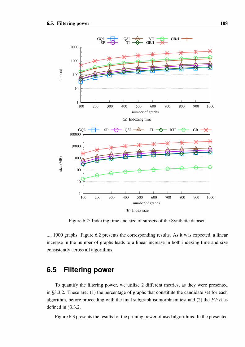
6.5. Filtering power 108
1
10
100
1000
10000
100 200 300 400 500 600 700 800 900 1000
tim
e (s
)
number of graphs
GQLSP
QSITI
BTIGR/1
GR/4
(a) Indexing time
1
10
100
1000
10000
100000
100 200 300 400 500 600 700 800 900 1000
size
(M
B)
number of graphs
GQL SP QSI TI BTI GR
(b) Index size
Figure 6.2: Indexing time and size of subsets of the Synthetic dataset
..., 1000 graphs. Figure 6.2 presents the corresponding results. As it was expected, a linearincrease in the number of graphs leads to a linear increase in both indexing time and sizeconsistently across all algorithms.
6.5 Filtering power
To quantify the filtering power, we utilize 2 different metrics, as they were presentedin §3.3.2. These are: (1) the percentage of graphs that constitute the candidate set for eachalgorithm, before proceeding with the final subgraph isomorphism test and (2) the FPR asdefined in §3.3.2.
Figure 6.3 presents the results for the pruning power of used algorithms. In the presented

6.5. Filtering power 109
0
20
40
60
80
100
avg
% g
rap
hs
GQL_CSS SP_CSS GR_CSS ASS
SyntheticPPIPCMPDBS
(a) Candidate and answer sets for all algorithms
0
0.2
0.4
0.6
0.8
1
fals
e p
osi
tiv
e ra
tio
GQL SP GR
SyntheticPPIPCMPDBS
(b) False Positive Ratio
Figure 6.3: Pruning Power of Grapes and SI methods
figures, CSS stands for Candidate Set Size and ASS stands for Answer Set Size. QuickSI,TurboIso, and BTI are not included in the presented results as they do not perform anyfiltering and they proceed directly with the subgraph isomorphism test. Grapes provides thesame filtering power independently of the number of threads that are executed and thus on thecorresponding figures we do not distinguish the results. For comparison purposes, we reportthe percentage of graphs that constitute the average answer set size along with the percentageof graphs that constitute the average candidate set size for each algorithm in figure 6.3(a).
In the aforementioned figures, we observe that different number of graphs were filteredout by the three different methods. Although it is not presented in the above figures, thefiltering power of the SI methods is slightly improved as the query size increases and thesame effect holds for Grapes. In the majority of cases, Grapes was able to filter out at least

6.6. Performance of SI methods 110
double the amount of graphs compared to GraphQL and sPath, leading to candidate sets veryclose to the actual answer set, and this is also evident in the low FPR. However, Grapes’filtering comes at an extra cost of a much larger index to store and more time to construct(see §6.3.2), with the sole exception of PDBS. sPath, that constructs a slightly more elaborateindex compared to GraphQL, was also able to achieve an up to 10% better filtering thanGraphQL. A very interesting observation is the fact that in very rare cases the graphs thatwere filtered out by the SI methods were not always a subset of the graphs filtered out byGrapes. This occurred in <1% of graph-query pairs and was more evident when increasingthe query size. Finally, it is important to observe the FPR in combination with the candidateset and answer set sizes. To showcase this, we note that although PDBS is the only datasetwhere the average candidate set sizes are among the biggest for all 3 algorithms reported, thecorresponding FPR are the lowest for all datasets because of the high answer set size.
6.6 Performance of SI methods
SI methods keep gaining ground over FTV methods, with the current tendency in recentwork to totally dismiss FTV methods with the claim that the smart subgraph isomorphismheuristics of the SI methods outperform the index-based FTV methods. Before proceedingwith further investigating this claim, we provide in figure 6.4 a head-to-head comparisonof the average query execution time of SI algorithms across all datasets. Because of therestriction mentioned in §6.3.2, for TurboIso and for PPI and Synthetic dataset only resultswith queries ≤ 24 edges are presented.
1
10
100
1000
10000
100000
1x10⁶
avg
qu
ery
ex
ec t
ime
(ms)
GQL SP QSI TI BTI
SyntheticPPIPCMPDBS
Figure 6.4: Avg query exec time (ms) of SI methods
As it can be seen from figure 6.4, there is no winner algorithm across all datasets. Thisfinding comes in agreement with [8] and our experiments in chapter §5, where for the SI

6.6. Performance of SI methods 111
algorithms the tested dataset contained only a single, large graph. TurboIso and BTI, thenewest additions in the set of SI algorithms, are favored particularly in datasets consistingof a small number of labels because of the smart rewritings applied on the query graph (andon the stored graph in the case of BTI). The least promising SI algorithm is QuickSI, butoutperforms BTI on PPI where the number of distinct labels is more abundant.
100
1000
10000
100000
1x10⁶
16 20 24 32
avg
qu
ery
ex
ec t
ime
(ms)
query size (# of edges)
GQL SP QSI TI BTI
(a) PPI
1000
10000
100000
1x10⁶
24 32 40
avg
qu
ery
ex
ec t
ime
(ms)
query size (# of edges)
GQL SP QSI TI BTI
(b) Synthetic
Figure 6.5: Avg query exec time (ms) of SI methods for PPI and Synthetic datasets and fordifferent query sizes
As we increase the query size, query processing becomes harder for all algorithms, withthe exception of PDBS and PCM where there are no significant differences for differentquery sizes. The relevant results for the PPI and the Synthetic dataset can be seen in figure6.5. It is worth mentioning that there is not a single winning algorithm for different querysizes even for the same dataset; this is consistent with both the findings in [10] and the resultspresented in §5.4.

6.7. Evaluating the hybrid FTV-SI method 112
6.7 Evaluating the hybrid FTV-SI method
Having discussed that the filtering of Grapes is more powerful than that achieved bythe SI methods, we set out to construct a hybrid FTV-SI solution. The proposed hybridsolution works as follows: We construct the index for both Grapes (the in use FTV method)and for the in use SI method. In the query processing, we perform the filtering of Grapes(as discussed in §3.1.1) and till the stage of forming the candidate set. Subsequently, forthose graphs that pass the filtering stage we use GraphQL/ sPath/ QuickSI/ TurboIso/ BTI,instead of Grapes’s default (and expensive) VF2 subgraph isomorphism test. Since an extrafiltering step is introduced (namely, the filtering from Grapes), it is worthwhile evaluating,analyzing, and quantifying the effect of the cost to perform this additional on-line filtering onthe overall achievable performance. As Grapes was originally designed to work in parallel,we utilize (·)/N to denote the in use number of threads N for Grapes-[GraphQL/ sPath/QuickSI/ TurboIso/ BTI] as the FTV-SI combination of algorithms. In this section we utilizeonly one thread; additional parallelism will be discussed in the following section. Last, forthe rest of the discussion, we assume that the indices are already loaded into main memoryonce at the beginning of the execution for each query workload.
6.7.1 Performance Metrics
For every query against a dataset of graphs, we measure the execution time, while avg
exec time denotes the average execution time. For the SI methods the execution time in-cludes the time for constructing the index of the query, the matching of the query’s index tothe databases’ index (where applicable) and the time required to perform the subgraph iso-morphism test. For our proposed hybrid FTV-SI solution the execution time includes (i) thetime required to perform the filtering of Grapes as described in §3.1.1 and (ii) the executiontime of the in use SI method for the graphs that passed the filtering stage (that substitutes theVF2 verification algorithm).
Let qi be a given query. Let also tMi be the execution time of qi over methodM , whereMcan be one of the SI methods, i.e., GraphQL/ sPath/ QuickSI/ TurboIso/ BTI, and tGrapes−M
i
be the execution time of qi over the hybrid combination of Grapes with method M over allthe graphs in the dataset. In order to evaluate the performance of this combination, we utilizethe speedup∗ metric defined as: tMi
tGrapes−Mi
. speedup∗ represents what we lose in performanceif we choose the original method over the various alternatives; i.e., speedup∗ equals themaximum attainable speedup over the original method, if we chose the best of the examinedalternatives. As we described in §3.3.4, the aforementioned speedup∗ metric can have a QLAand WLA version, denoted with a matching subscript; e.g. speedup∗QLA.

6.7. Evaluating the hybrid FTV-SI method 113
6.7.2 Performance Results
Before proceeding with the presentation of the achieved speedups, we initially discussthe indexing costs we need to pay for our hybrid FTV-SI solution. Thus, the size of theconstructed index for all datasets for the hybrid FTV-SI solution is the addition of Grapes’index with the index of the in use SI method as presented in figure 6.1(b). The same holdsfor the corresponding indexing times. The pruning power of the FTV-SI solution is equalto the pruning power of Grapes, as it was presented in figure 6.3 and for the correspondingdatasets.
0
1
2
3
4
5
6
7
8
9
10
avg
sp
eed
up
*Q
LA
(GR-GQL)/1(GR-SP)/1
(GR-QSI)/1(GR-TI)/1
(GR-BTI)/1
SyntheticPPIPCMPDBS
(a) Average speedup∗QLA
0
1
2
3
4
5
6
avg
sp
eed
up
*W
LA
(GR-GQL)/1(GR-SP)/1
(GR-QSI)/1(GR-TI)/1
(GR-BTI)/1
SyntheticPPIPCMPDBS
(b) Average speedup∗WLA
Figure 6.6: Average speedup∗QLA & speedup∗WLA of the hybrid FTV-SI method
Figure 6.6 presents the average QLA and WLA speedups for all datasets and query sizes.We were not able to execute queries >25 vertices with TurboIso (§6.3.2); as a result in PPIand the Synthetic dataset the presented speedup for the hybrid Grapes-TurboIso combination

6.7. Evaluating the hybrid FTV-SI method 114
(GR-GQL)/1 (GR-SP)/1 (GR-QSI)/1 (GR-TI)/1 (GR-BTI)/1
PDB
S
stdDev 1.783 2.035 2.589 1.556 0.456min 0.777 0.798 0.847 0.682 0.022max 10.361 12.179 15.185 9.107 3.055
median 1.937 1.934 2.119 1.915 0.308PC
M
stdDev 3.454 3.093 6.560 3.655 0.218min 1.164 1.182 1.250 1.195 0.053max 14.912 14.029 26.001 17.099 1.078
median 5.436 5.153 6.975 5.619 0.776
PPI
stdDev 2.886 7.112 37.603 2.852 119.611min 0.857 0.914 0.001 0.877 0.067max 24.196 29.198 89.884 18.479 90.6
median 1.496 1.416 1.522 1.865 0.993
Synt
hetic
stdDev 5.465 9.444 21.386 2.248 15.599min 1.269 1.094 1.168 1.633 0.292max 28.554 65.586 29.042 12.920 61.415
median 5.107 3.683 2.777 2.649 0.964
Table 6.1: speedup∗QLA statistics for FTV-SI combination with 1 thread
refers to queries ≤ 24 edges, and thus results are not directly comparable with the rest of theresults for the hybrid Grapes-M combinations. BTI is the sole algorithm that is rather hurtthan improved by this hybrid combination in PCM where the size of data graphs is relativelysmall, and in PDBS where the size of the candidate graphs in the dataset is relatively high.In the majority of cases the achieved speedups are higher as the query size increases andthis effect is more profound in the Synthetic dataset, because of the much higher numberof graphs that constitute the Synthetic dataset and the higher percentages of graphs thatwere filtered out (as we can observe in combination with figure 6.3(a)). To showcase this,we provide in figure 6.7 the average query execution times of the hybrid FTV-SI methodsfor PPI and Synthetic datasets and for different query sizes that can be compared againstthe average query execution times of the hybrid SI methods for the same datasets (figure6.5). In other words, the query graphs in the Synthetic dataset provide better selectivity thanthose in the 3 Real datasets and this is reflected in the achieved speedups. A notable fact,presented in figure 6.8, is that the different achieved speedups for all algorithms bring aboutsignificant changes in their average query execution times, as they were presented in figure6.4. However, not a single winner algorithm across all datasets and different query sizes isyet identified!
Table 6.1 presents additional statistics for min, max, median and stdDev of the achievedspeedup∗QLA. For all algorithms except for BTI, we observe that the min achieved speedupis not always > 1, but the median speedup∗QLA is in all cases > 1. In other words, thereare some queries that the time gained from the filtered out graphs does not pay off. For theexecuted queries, this phenomenon occurred when the candidate set size was ≥ 500 graphs

6.8. Reducing filtering time with parallelism 115
100
1000
10000
100000
1x10⁶
16 20 24 32
avg
qu
ery
ex
ec t
ime
(ms)
query size (# of edges)
(GR-GQL)/1(GR-SP)/1
(GR-QSI)/1(GR-TI)/1
(GR-BTI)/1
(a) PPI
1000
10000
100000
1x10⁶
24 32 40
avg
qu
ery
ex
ec t
ime
(ms)
query size (# of edges)
(GR-GQL)/1(GR-SP)/1
(GR-QSI)/1(GR-TI)/1
(GR-BTI)/1
(b) Synthetic
Figure 6.7: Avg query exec time (ms) of hybrid FTV-SI methods for PPI and Syntheticdatasets and for different query sizes
in PDBS and ≥ 15 graphs in PPI.
6.8 Reducing filtering time with parallelism
As Grapes was designed to work in parallel, we studied this effect with additional ex-periments. Specifically, we used Grapes/4 for the filtering stage, alongside one of the SIalgorithms, on the same set of datasets and query workloads. We utilize as many differ-ent (parallel) instances of SI algorithms as the number of threads N utilized by Grapes. Wemaintain the graphs that passed Grapes’ filtering test in a queue and the firstN graphs are as-signed to theN threads. Till the graph queue is empty, the first graph in the queue is assigned

6.8. Reducing filtering time with parallelism 116
1
10
100
1000
10000
100000
1x10⁶
avg
qu
ery
ex
ec t
ime
(ms)
(GR-GQL)/1(GR-SP)/1
(GR-QSI)/1(GR-TI)/1
(GR-BTI)/1
SyntheticPPIPCMPDBS
Figure 6.8: Avg query exec time (ms) of the FTV-SI hybrid methods
to the next available thread. This choice brings additional performance improvement.
Figure 6.9: Example on parallel execution of the verification stage of the hybrid FTV-SIcombination with number of threads N = 2. (We assume that graphs g1, g2, g4, and g8
formed the candidate set after the filtering stage. The red X is used to represent the removalof a grpah from the queue or the completion of a thread execution.)
To showcase this, we will additionally present an example (figure 6.9). We assume thatwe use N = 2 threads and that after the filtering stage of Grapes the candidate set is formedby graphs g1, g2, g4 and g8. Thus, in the verification stage and at time t0, g1, g2, g4, andg8 are placed in a queue. We also instantiate as many different instances of the in use SImethod as the number of threads N to run in parallel, denoted T#i, where i = 0, ..., N − 1.
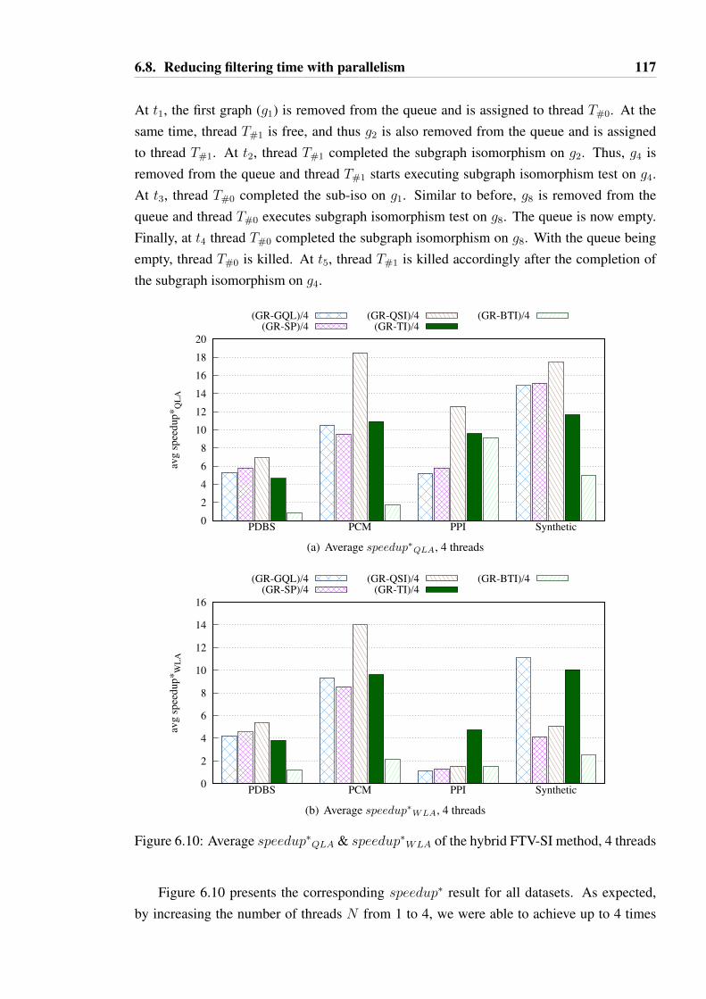
6.8. Reducing filtering time with parallelism 117
At t1, the first graph (g1) is removed from the queue and is assigned to thread T#0. At thesame time, thread T#1 is free, and thus g2 is also removed from the queue and is assignedto thread T#1. At t2, thread T#1 completed the subgraph isomorphism on g2. Thus, g4 isremoved from the queue and thread T#1 starts executing subgraph isomorphism test on g4.At t3, thread T#0 completed the sub-iso on g1. Similar to before, g8 is removed from thequeue and thread T#0 executes subgraph isomorphism test on g8. The queue is now empty.Finally, at t4 thread T#0 completed the subgraph isomorphism on g8. With the queue beingempty, thread T#0 is killed. At t5, thread T#1 is killed accordingly after the completion ofthe subgraph isomorphism on g4.
0
2
4
6
8
10
12
14
16
18
20
avg
sp
eed
up
*Q
LA
(GR-GQL)/4(GR-SP)/4
(GR-QSI)/4(GR-TI)/4
(GR-BTI)/4
SyntheticPPIPCMPDBS
(a) Average speedup∗QLA, 4 threads
0
2
4
6
8
10
12
14
16
avg
sp
eed
up
*W
LA
(GR-GQL)/4(GR-SP)/4
(GR-QSI)/4(GR-TI)/4
(GR-BTI)/4
SyntheticPPIPCMPDBS
(b) Average speedup∗WLA, 4 threads
Figure 6.10: Average speedup∗QLA & speedup∗WLA of the hybrid FTV-SI method, 4 threads
Figure 6.10 presents the corresponding speedup∗ result for all datasets. As expected,by increasing the number of threads N from 1 to 4, we were able to achieve up to 4 times

6.9. Index Time/Size - Filtering Power Tradeoff 118
(GR-GQL)/4 (GR-SP)/4 (GR-QSI)/4 (GR-TI)/4 (GR-BTI)/4
PDB
S
stdDev 2.393 2.838 4.067 2.022 0.829min 1.794 1.924 2.201 1.353 0.022max 13.988 16.847 23.709 11.568 4.278
median 5.250 5.616 6.585 4.770 0.397PC
M
stdDev 3.397 2.925 8.550 3.603 0.901min 3.579 3.521 4.453 3.776 0.054max 18.425 17.255 40.317 21.375 3.475
median 10.298 9.435 17.664 10.838 1.721
PPI
stdDev 3.280 16.967 61.712 7.481 134.922min 1.001 1.003 1.003 3.403 0.0893max 26.366 5.613 85.818 63.498 297.41
median 4.511 4.278 4.409 7.001 1.704
Synt
hetic
stdDev 6.184 12.819 30.828 6.639 22.757min 1.318 1.134 1.636 6.153 0.330max 31.975 108.596 96.647 30.388 72.763
median 13.613 10.892 8.913 9.491 3.342
Table 6.2: speedup∗QLA statistics for FTV-SI combination with 4 threads
better speedups compared to the single-threaded executions. Table 6.2 presents additionalstatistics for min, max, median and stdDev of the achieved speedup∗QLA in the case of 4threads, where in all datasets and query workloads the achieved speedup is > 1.
6.9 Index Time/Size - Filtering Power Tradeoff
In our discussion so far we used the default values of the enumerated features for con-structing the index for Grapes, as suggested by the respective authors. But as we have seen,the constructed index of FTV methods is costly both in size and in time. In this section wetweak the size of the enumerated featuresmaxL (see §3.1.1) and we observe the filtering thatcan be achieved and how this affects the gained speedups in our hybrid proposed solution.Thus, for our experiments we have used maxL = 2, 3, 4, 5. We report that for maxL = 5,the index process was utilizing excessive amount of memory, leading to thrashing even to our128GB machine and thus no numbers are reported for this case. In the subsequent figures,we utilize Grapes-Li, i = 2, 3, 4 (or GR-Li for short) to denote the maxL value used.
Figures 6.11(a) and 6.11(b) report the indexing time and size for Grapes and the dif-ferent maxL tried for all employed datasets. For comparison, we additionally include thecorresponding values for the employed SI methods. For all datasets, except for PDBS, thereis a difference of up to 3 orders of magnitude for both indexing time and size and for maxLfrom 2 to 4, leading to times and sizes much smaller than the SI methods in most cases. ForPDBS, the small number of labels and thus the small variation of enumerated paths leads to

6.9. Index Time/Size - Filtering Power Tradeoff 119
0.1
1
10
100
1000
10000
tim
e (s
)
GQLSP
QSI
TIBTI
(GR-L2)/1
(GR-L2)/4(GR-L3)/1(GR-L3)/4
(GR-L4)/1(GR-L4)/4
SyntheticPPIPCMPDBS
(a) Indexing Time
1
10
100
1000
10000
100000
size
(M
B)
GQLSP
QSITI
BTIGR-L2
GR-L3GR-L4
SyntheticPPIPCMPDBS
(b) Indexing Size
Figure 6.11: Tweaking the maxL parameter, index construction
up to 1 order of magnitude difference of the index size from maxL = 2 to 4. Thus, overallin the hybrid FTV-SI method, the use of smaller maxL values results in adding only a trivialtime and space overhead in the indexing phase.
Figures 6.12(a) and 6.12(b) present the pruning power of Grapes utilizing different fea-ture sizes on all datasets. As it was expected, as we increase the size of the features, thecandidate set size decreases and it affects accordingly the FPR. However, in all occasionsthe filtering power is better than that achieved by the SI methods. This is particularly evidentin PPI, PCM and the Synthetic dataset. For these datasets and for all feature sizes, the candi-date set size is very close to the answer set size. Thus, we also obtain relatively small FPRvalues. PDBS follows the same trends but with less steep divergence from the SI methodsbecause of the high answer set size. This leads to the conclusion that we can still achieve

6.9. Index Time/Size - Filtering Power Tradeoff 120
0
20
40
60
80
100
avg
% g
rap
hs
GQL_CSSSP_CSS
GR-L2_CSSGR-L3_CSS
GR-L4_CSSASS
SyntheticPPIPCMPDBS
(a) Candidate and answer sets
0
0.2
0.4
0.6
0.8
1
fals
e p
osi
tiv
e ra
tio
GQL SP GR-L2 GR-L3 GR-L4
SyntheticPPIPCMPDBS
(b) False Positive Ratio
Figure 6.12: Tweaking the maxL parameter, filtering power
high speedups with smaller feature sizes.
Finally, figures 6.13(c) - 6.14(f) report the achieved QLA and WLA speedups by tweak-ing the maxL value of Grapes for the used datasets for our hybrid FTV-SI solution whenutilizing 1 and 4 threads and for all query sizes. A notable observation here is that in somecases, with the sole exception of PDBS and PCM, the achieved speedups with smaller valuesof maxL outperform the speedups with larger values of maxL. We attribute this to the factthat for smaller maxL values less time is required to construct the index of the query andmatch it to the dataset’s index. Additionally, the fact that the candidate set sizes that areformed after Grapes’s filtering are close for the various maxL values, contributes to this.For completeness, tables 6.3 and 6.4 provide additional statistics for min, max, median andstdDev of the achieved speedup∗QLA with different feature sizes and different number of

6.9. Index Time/Size - Filtering Power Tradeoff 121
0 2 4 6 8
10
12
14
avg speedup*QLA
(GR
-L2 -
GQ
L)/
1(G
R-L
2 -
SP
)/1
(GR
-L2 -
QS
I)/1
(GR
-L2 -
TI)
/1(G
R-L
2 -
BT
I)/1
Sy
nth
etic
PP
IP
CM
PD
BS
(a)
Avg
speedup∗ Q
LA
,maxL
=2,
1th
read
0 2 4 6 8
10
12
14
avg speedup*QLA
(GR
-L3 -
GQ
L)/
1(G
R-L
3 -
SP
)/1
(GR
-L3 -
QS
I)/1
(GR
-L3 -
TI)
/1(G
R-L
3 -
BT
I)/1
Sy
nth
etic
PP
IP
CM
PD
BS
(b)
Avg
speedup∗ Q
LA
,maxL
=3,
1th
read
0 2 4 6 8
10
12
14
avg speedup*QLA
(GR
-L4 -
GQ
LI)
/1(G
R-L
4 -
SP
)/1
(GR
-L4 -
QS
I)/1
(GR
-L4 -
TI)
/1(G
R-L
4 -
BT
I)/1
Sy
nth
etic
PP
IP
CM
PD
BS
(c)
Avg
speedup∗ Q
LA
,maxL
=4,
1th
read
0 1 2 3 4 5 6
avg speedup*WLA
(GR
-L2 -
GQ
L)/
1(G
R-L
2 -
SP
)/1
(GR
-L2 -
QS
I)/1
(GR
-L2 -
TI)
/1(G
R-L
2 -
BT
I)/1
Sy
nth
etic
PP
IP
CM
PD
BS
(d)
Avg
speedup∗ W
LA
,maxL
=2,
1th
read
0 1 2 3 4 5 6
avg speedup*WLA
(GR
-L3 -
GQ
L)/
1(G
R-L
3 -
SP
)/1
(GR
-L3 -
QS
I)/1
(GR
-L3 -
TI)
/1(G
R-L
3 -
BT
I)/1
Sy
nth
etic
PP
IP
CM
PD
BS
(e)
Avg
speedup∗ W
LA
,maxL
=3,
1th
read
0 1 2 3 4 5 6
avg speedup*WLA
(GR
-L4 -
GQ
LI)
/1(G
R-L
4 -
SP
)/1
(GR
-L4 -
QS
I)/1
(GR
-L4 -
TI)
/1(G
R-L
4 -
BT
I)/1
Sy
nth
etic
PP
IP
CM
PD
BS
(f)
Avg
speedup∗ W
LA
,maxL
=4,
1th
read
Figu
re6.
13:T
wea
king
the
max
Lpa
ram
eter
,ach
ieve
dspeedup∗
,1th
read

6.9. Index Time/Size - Filtering Power Tradeoff 122
0 5
10
15
20
25
30
avg speedup*QLA
(GR
-L2 -
GQ
L)/
4(G
R-L
2 -
SP
)/4
(GR
-L2 -
QS
I)/4
(GR
-L2 -
TI)
/4(G
R-L
2 -
BT
I)/4
Sy
nth
etic
PP
IP
CM
PD
BS
(a)
Avg
speedup∗ Q
LA
,maxL
=2
0 5
10
15
20
25
30
avg speedup*QLA
(GR
-L3 -
GQ
L)/
4(G
R-L
3 -
SP
)/4
(GR
-L3 -
QS
I)/4
(GR
-L3 -
TI)
/4(G
R-L
3 -
BT
I)/4
Sy
nth
etic
PP
IP
CM
PD
BS
(b)
Avg
speedup∗ Q
LA
,maxL
=3
0 5
10
15
20
25
30
avg speedup*QLA
(GR
-L4 -
GQ
LI)
/4(G
R-L
4 -
SP
)/4
(GR
-L4 -
QS
I)/4
(GR
-L4 -
TI)
/4(G
R-L
4 -
BT
I)/4
Sy
nth
etic
PP
IP
CM
PD
BS
(c)
Avg
speedup∗ Q
LA
,maxL
=4
0 2 4 6 8
10
12
14
16
avg speedup*WLA
(GR
-L2 -
GQ
L)/
4(G
R-L
2 -
SP
)/4
(GR
-L2 -
QS
I)/4
(GR
-L2 -
TI)
/4(G
R-L
2 -
BT
I)/4
Sy
nth
etic
PP
IP
CM
PD
BS
(d)
Avg
speedup∗ W
LA
,maxL
=2
0 2 4 6 8
10
12
14
16
avg speedup*WLA
(GR
-L3 -
GQ
L)/
4(G
R-L
3 -
SP
)/4
(GR
-L3 -
QS
I)/4
(GR
-L3 -
TI)
/4(G
R-L
3 -
BT
I)/4
Sy
nth
etic
PP
IP
CM
PD
BS
(e)
Avg
speedup∗ W
LA
,maxL
=3
0 2 4 6 8
10
12
14
16
avg speedup*WLA
(GR
-L4 -
GQ
LI)
/4(G
R-L
4 -
SP
)/4
(GR
-L4 -
QS
I)/4
(GR
-L4 -
TI)
/4(G
R-L
4 -
BT
I)/4
Sy
nth
etic
PP
IP
CM
PD
BS
(f)
Avg
speedup∗ W
LA
,maxL
=4
Figu
re6.
14:T
wea
king
the
max
Lpa
ram
eter
,ach
ieve
dspeedup∗
,4th
read
s

6.9. Index Time/Size - Filtering Power Tradeoff 123
1th
read
4th
read
sG
R-G
QL
GR
-SP
GR
-QSI
GR
-TI
GR
-BT
IG
R-G
QL
GR
-SP
GR
-QSI
GR
-TI
GR
-BT
I
PDBS
stdD
ev1.
481
1.68
92.
185
1.33
20.
215
2.25
32.
612
3.66
92.
024
0.41
8m
in0.
581
0.60
70.
688
0.48
50.
021
1.01
91.
104
1.37
00.
748
0.02
1m
ax9.
712
11.8
5316
.612
8.83
80.
849
12.7
5816
.189
22.3
7510
.904
1.60
8m
edia
n1.
687
1.78
11.
893
1.64
30.
251
4.22
54.
706
5.58
73.
789
0.30
8
PCM
stdD
ev2.
509
2.24
74.
864
2.66
10.
221
2.37
82.
047
6.29
22.
556
0.82
2m
in1.
049
1.03
91.
101
1.03
00.
042
3.17
33.
070
3.80
82.
981
0.04
3m
ax11
.155
10.0
2221
.071
12.2
031.
050
13.4
6811
.685
29.3
7214
.227
3.24
2m
edia
n4.
008
3.69
04.
891
4.11
90.
710
7.56
96.
896
12.7
127.
959
1.44
0
PPI
stdD
ev3.
515
6.06
036
.828
3.23
415
1.38
53.
563
11.6
0654
.506
8.72
815
1.34
6m
in0.
832
0.88
90.
910
0.84
60.
081
1.00
11.
003
1.00
22.
201
0.08
1m
ax30
.759
8.57
498
.490
22.1
0422
5.01
030
.759
7.71
689
.218
71.1
0332
5.01
med
ian
1.36
41.
301
1.38
51.
640
0.99
23.
298
3.39
33.
380
4.56
01.
613
Synthetic
stdD
ev8.
549
13.6
6722
.341
1.90
121
.319
9.23
816
.897
38.4
265.
134
30.5
81m
in1.
260
1.09
21.
105
1.53
30.
474
1.31
51.
135
1.63
65.
342
0.47
6m
ax51
.635
101.
997
37.1
7910
.595
62.1
3954
.019
123.
504
112.
209
29.8
1259
.015
med
ian
4.29
23.
145
2.32
52.
281
0.97
211
.796
9.05
47.
566
8.04
33.
299
Tabl
e6.
3:speedup∗
QLA
stat
istic
sfo
rFT
V-S
Icom
bina
tion
with
1an
d4
thre
ads,maxL
=2
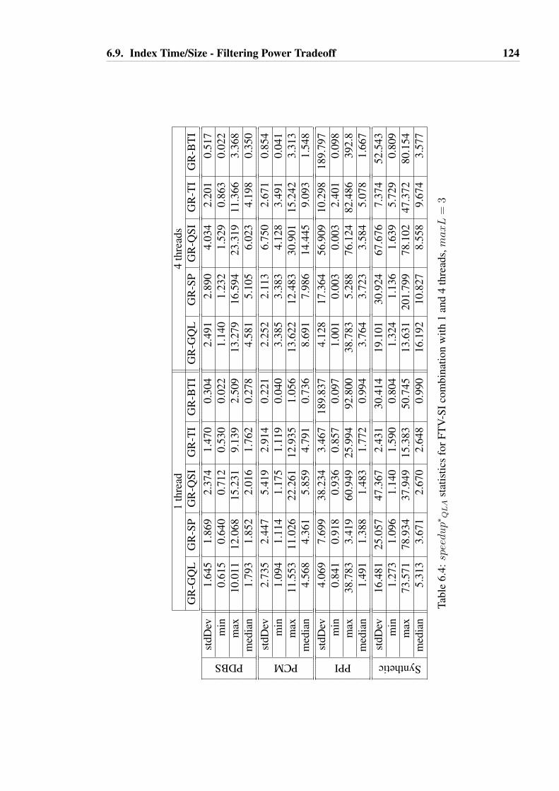
6.9. Index Time/Size - Filtering Power Tradeoff 124
1th
read
4th
read
sG
R-G
QL
GR
-SP
GR
-QSI
GR
-TI
GR
-BT
IG
R-G
QL
GR
-SP
GR
-QSI
GR
-TI
GR
-BT
I
PDBS
stdD
ev1.
645
1.86
92.
374
1.47
00.
304
2.49
12.
890
4.03
42.
201
0.51
7m
in0.
615
0.64
00.
712
0.53
00.
022
1.14
01.
232
1.52
90.
863
0.02
2m
ax10
.011
12.0
6815
.231
9.13
92.
509
13.2
7916
.594
23.3
1911
.366
3.36
8m
edia
n1.
793
1.85
22.
016
1.76
20.
278
4.58
15.
105
6.02
34.
198
0.35
0
PCM
stdD
ev2.
735
2.44
75.
419
2.91
40.
221
2.25
22.
113
6.75
02.
671
0.85
4m
in1.
094
1.11
41.
175
1.11
90.
040
3.38
53.
383
4.12
83.
491
0.04
1m
ax11
.553
11.0
2622
.261
12.9
351.
056
13.6
2212
.483
30.9
0115
.242
3.31
3m
edia
n4.
568
4.36
15.
859
4.79
10.
736
8.69
17.
986
14.4
459.
093
1.54
8
PPI
stdD
ev4.
069
7.69
938
.234
3.46
718
9.83
74.
128
17.3
6456
.909
10.2
9818
9.79
7m
in0.
841
0.91
80.
936
0.85
70.
097
1.00
10.
003
0.00
32.
401
0.09
8m
ax38
.783
3.41
960
.949
25.9
9492
.800
38.7
835.
288
76.1
2482
.486
392.
8m
edia
n1.
491
1.38
81.
483
1.77
20.
994
3.76
43.
723
3.58
45.
078
1.66
7
Synthetic
stdD
ev16
.481
25.0
5747
.367
2.43
130
.414
19.1
0130
.924
67.6
767.
374
52.5
43m
in1.
273
1.09
61.
140
1.59
00.
804
1.32
41.
136
1.63
95.
729
0.80
9m
ax73
.571
78.9
3437
.949
15.3
8350
.745
13.6
3120
1.79
978
.102
47.3
7280
.154
med
ian
5.31
33.
671
2.67
02.
648
0.99
016
.192
10.8
278.
558
9.67
43.
577
Tabl
e6.
4:speedup∗
QLA
stat
istic
sfo
rFT
V-S
Icom
bina
tion
with
1an
d4
thre
ads,maxL
=3

6.10. Conclusions 125
threads and along with tables 6.1 and 6.2 (presented earlier in§6.7 and §6.8) complete thepicture. We note that BTI is again the least benefited algorithm, as evident in the retrievedvalues of average, min and median speedup∗QLA values. In fact it is rather harmed than im-proved by the use of smaller feature sizes, i.e., maxL = 2 or maxL = 3 in the vast majorityof cases. In PDBS particularly, BTI with the use of smaller feature sizes is not even benefitedby the use of 4 threads.
Undoubtedly, the aforementioned speedups bring about additional changes in the aver-age query execution times, as discussed earlier in §6.7. Thus, the overall conclusion, with thesole exception of BTI, is that the use of smaller feature sizes in the hybrid FTV-SI method isnot just a good compromise of the achieved speedups. This solution offers additional bene-fits in the indexing phase by reducing significantly both the index size and time, as discussedearlier in this section.
6.10 Conclusions
The current trend in research for subgraph pattern queries in graph DBs dismisses FTVmethods since the fast subgraph isomorphism heuristics of SI methods significantly outper-form FTV methods. We analyzed the problem by answering a set of fundamental questions.Specifically, we initially investigated the index time and space requirements from both FTVand SI methods. Subsequently, we showed that the filtering power of a top-performing FTValgorithm (Grapes) is significantly better than that of all SI methods. Having that in mind andknowing that the subgraph isomorphism testing can be very expensive as the graph DB growslarge (in number or size of stored graphs), we set out to initially evaluate the performanceof well known SI methods. Our experiments reveal no single winner across all datasets. Wethen evaluate the performance of a hybrid FTV-SI solution, that incorporates the powerfulfiltering of the FTV methods with the fast subgraph-isomorphism algorithm of the SI meth-ods. This hybrid proves to be a better practice compared to the traditional SI methods overdatasets consisting of a large number of graphs by avoiding redundant and possibly expensivesub-iso tests in the whole DB, and thus by bringing about significant speedups and changesin algorithms’ relative performance with not yet a single winner. However, gained benefitscome at the extra costs of index memory space and indexing time. We then further analyzedthis hybrid method in two dimensions: First, to reduce the space-time index costs, we low-ered the size of indexed features. Our results revealed that the filtering power of the FTVindex is still much higher than that of SI methods and that high speedups can be achieved,even with these smaller indexes, which are in turn even smaller than the SI indexes. Second,as the time to perform index-based filtering is substantial, we studied the positive effects ofdoing this in parallel. Our results showed that expected speedups can thus be significantly

6.10. Conclusions 126
boosted. Parallelizing this filtering step is a much easier task than parallelizing the actualsubgraph-isomorphism algorithm. Overall, this work surfaces new promising possibilitiesfor expediting subgraph queries in graph DBs by experimentally revealing a blind spot incurrent thinking. We hope this will inspire new research targeting new FTV-style indexesand/or SI-style subgraph-isomorphism algorithms for FTV-SI hybrids.
Limitations The current work is limited to the use of three real and a synthetic datasets.A systematic study, as performed in chapter §4, would be useful to (i) perform a systematicevaluation of existing SI algorithms and the hybrid FTV-SI method and (ii) pinpoint thescalability limitations. Regarding the scalability limits, we also need to identify the existenceof straggler-queries (as discussed in chapter §5). Then, we could combine the Ψ-framework(§5.8) and the hybrid FTV-SI combination method (§6.7 and §6.8) to extend the scalabilitylimitations of the originally proposed FTV and SI methods. This will be further discussed in§7.2.
Another limitation of our study is related to the values of the input parameters of theemployed SI algorithms (see §4.3.2). We would expect that varying the input parameters onthe SI methods (see §6.3.2) would have similar effects as varying the input parameters on theFTV methods (see §6.9).

127
Chapter 7
Conclusion and Future Steps
[ X \
After numerous experiments and all the knowledge we have gained so far, we are readyto conclude this thesis. In the current chapter, we briefly review our findings and our majorcontributions. Of course, there are still open questions and space for improvement. Thus, inthe end we set the future steps to be conducted.
7.1 Summary of Contributions
Graphs have great representation power in representing complex structures and theirinteractions. A common problem that is addressed to such graphs is the subgraph patternmatching problem. Over the years, significant work has been conducted in the field of sub-graph matching queries, which entails subgraph isomorphism, a well-known NP-Completeproblem. Related work, that was extensively discussed in chapter §2, is classified in two ma-jor categories: the FTV methods that typically address the decision version, and SI methodsthat usually address the matching version of the problem. We have seen that a number ofsuch methods is added in the bibliography annually, that tend to totally dismiss older pro-posed methods and instead present new ideas with the aim to surpass the performance offormer work. With our experiments, we show that both FTV and SI methods show signifi-cant limitations in their performance as we were increasing the parameters of the problem,i.e. the number of nodes and / or density per graph, the number of graphs in the dataset,and the size of the query. Thus, in the current thesis we propose that instead of devisingnew algorithms, we should consider rewriting the original query and / or combining existing,top-performing algorithms appropriately in order to achieve large performance gains.

7.1. Summary of Contributions 128
More specifically, in chapter §4, we conducted a set of experiments with well-known andtop-performing FTV methods with an emphasis on newer proposed methods. We have em-ployed four real datasets and many synthetic ones, generated with the well-known GraphGen[60].We have identified a set of key-factor parameters that influence the performance of FTVmethods and in general the underlying subgraph isomorphism test and these are the num-ber of nodes and density per graph, the number of distinct labels and number of graphsin the dataset, along with the size of the query. The primary aim of our experiments wasto study their performance and sensitivity in the gradual increasing key-factor parameters(§4.4). Additionally, we stress-tested the various FTV methods by pinpointing points wheresome algorithms continue to operate whereas others break. Overall, from our analysis wegained the following insights:
• The first major lesson is related to the effect of the key dataset characteristics. Theintuition is verified; increasing the number of graphs (see figures 4.10 and 4.11) leadsto a linear increase in the problem’s complexity. The frequent mining techniques aremore severely affected, as more features have to be located across more graphs. Bycomplexity, we mean the indexing time and size and the query processing time. Byincreasing the number of nodes and density, the complexity increases in a super-linearway (see figures 4.3 and 4.4, 4.5 and 4.6). However, increasing the number of labelsleads to an easier problem, because there are more distinct features and the filteringworks better (see figures 4.8 and 4.9). Finally, by increasing the size of the queries,the query processing becomes harder, with the effect being more profound on densegraphs and specifically on frequent mining techniques (see figures 4.4, 4.6 and 4.11and §4.5.1).• The second major lesson is that simplicity wins (see §4.5.2). Many methods advo-
cate that graphs are more expressive than trees and trees are more expressive thanpaths accordingly, as graphs can maintain more structural information. We agree withthis claim. However, considering that all paths are trees but the opposite does nothold, given any graph in the dataset and similarly for graphs, the number of producedsubgraphs of the same size is higher than the number of trees of the same size andaccordingly for paths. If the methods utilizing more complex structures had to storeeverything, then the indexing time, index size and filtering time would be much higher.Thus, all methods employing complex structures maintain only a subset or apply en-coding (see description of gIndex, Tree+∆, gCode and CT-Index in §3.1.1). As aresult, their coverage is decreased, i.e., some features are not represented in the in-dex. On the other side, methods that rely on simpler features (paths), compared to thefrequent mining techniques can index all the features up to a certain size, in the costof an increased constructed index (Grapes and GGSX in figures 4.3(b), 4.5(b), 4.8(b)and 4.10(b)). In the end, exhaustive enumeration techniques have more or less the

7.1. Summary of Contributions 129
same behavior with frequent mining techniques in the filtering, but because of theirsimplicity, they win in both indexing and query processing time.• The choice of the right algorithm relies on optimizing different aspects of the prob-
lem and these are: efficiency in terms of indexing time, index size, query processingtime and scalability limitations. Based on our experiments, in most cases, Grapes andGGSX, utilizing the simplest features, are the winners, as discussed in §4.5.3. How-ever their index size requirements are the highest among all contestants.• In the relevant bibliography [7], all methods were tested with small and sparse datasets.
With our experiments, we have seen that at datasets consisting of larger and densergraphs, these algorithms do not scale. At larger scales, one should consider other op-tions such as devising new algorithms, varying the input parameters of top-performingmethods and/or combining existing top-performing algorithms to form a better one, asdiscussed in §4.5.4.
In chapter §5, we focused on the various subgraph isomorphism tests. We conducted aset of experiments with top-performing FTV, namely Grapes and GGSX, and SI methods,namely GraphQL, sPath, QuickSI, TurboIso and BTI, and we presented key novel discoveriesand observations of the nature of the subgraph isomorphism problem. Specifically, we madethe following key observations.
• Related works present the average query execution time, calculated as the query work-load time divided by the number of the queries in the workload to showcase the per-formance of their method compared to others. However, such an approach can concealthe real execution times of individual queries. Specifically, with our work we haveseen that as the dataset grows large in terms of number of nodes and/or density, queryprocessing becomes harder (see figures 5.1 and 5.3 and tables 5.1 and 5.2). We con-ducted experiments with a single query against a single large stored graph and we haveseen that both FTV and SI methods suffer from straggler queries, i.e., queries with ex-ecution times many orders of magnitude worse compared to the majority (see figures5.2 and 5.4). Straggler queries appear in a small percentage of the total query work-loads, but when execution times are averaged, the most expensive queries dominatethe overall processing time.• Isomorphic queries can have widely and wildly different execution times (see figures
5.5 and 5.7 and discussion in §5.5). We recall that for the generation of an isomorphicquery to the original query, one can simply permute the node IDs of the original query,as discussed in §2.2. The reason for that is that all proposed methods do not define anabsolutely strict order in which the nodes of the query are matched, because it wouldbe too computationally expensive to compute a globally optimal join plan. Instead,proposed methods rely on heuristics to minimize the search space for the join plan(§5.5). We have seen that FTV methods are more vulnerable to such wild variations

7.1. Summary of Contributions 130
as they propose a less strict order in which the nodes of the query are matched to thenodes of the stored graph compared to the SI methods.• Finally, we have seen that straggler queries are algorithm specific, i.e., a straggler
query on one algorithm could be a typical query on some other algorithm (figures5.15). For our experiments, we employed the various SI methods. We have seenthat the use of alternative algorithms is much more beneficial compared to the useof different isomorphic query rewritings, leading to straggler-free executions (figures5.14 and 5.15).
Many of the issues observed are encountered with other NP-hard problems, such asbranch and bound[116], as discussed in §2.7 and in §5.5, §5.8. We have seen that proposedalgorithms show a wide variance in their execution times as they employ different heuristicsand are significantly affected by the search order they impose. Additionally, the way theyresolve ties during their processing may further affect the search order, again resulting inunpredictable overall execution times.
Subsequently, we used our observations to make the following key contributions.
• We generated our own isomorphic query rewritings by permuting the query node IDsin a specific manner, as discussed in §5.6. Thus, we implemented and further experi-mented with 5 such rewritings, namely ILF, IND, DND, ILF+IND and ILF+DND thatpermute the node IDs in such a way that they take into consideration the frequenciesof labels of the stored graph and/or the query node degrees. With our experiments, wehave seen that these rewritings are beneficial across different algorithms and datasets(see figures 5.12 and 5.14).• We proposed and experimented with the Ψ-framework which stands for Parallel Sub-
graph Isomorphism Framework, as discussed in §5.8. Specifically, we run in paralleldifferent isomorphic instances of the same query and/or different algorithms by instan-tiating different threads. After the completion of any first thread, the rest of them arekilled. To reduce the memory footprint, we experimented with various combinationsand a number of threads. Such an execution leads to a performance improvement ofmany orders of magnitude compared to the original proposed methods.
Similar techniques to our Ψ-framework are applied to other NP-hard searches. Theseare known as portfolios of algorithms, as discussed in §2.7 and §5.8, where some portfoliospay-off more than others.
In chapter §6, we investigated the current trend that tends to totally dismiss FTV meth-ods and instead employ SI methods, with the claim that SI methods enjoy much shorterexecution times whereas FTV methods additionally suffer from elevated costs in managingtheir constructed index. Thus, we initially evaluated the performance of the aforementionedtop-performing SI methods over graph DBs consisting of a large number of graphs. Our

7.1. Summary of Contributions 131
experiments in featuring a single winner were inconclusive (see figure 6.4). In parallel, weinvestigated the time and size costs (figure 6.1) related to the constructed index of both theSI methods and Grapes – the top-performing FTV method in terms of indexing time, queryprocessing time, scalability limitations and filtering power, as shown in chapter §4 – alongwith the filtering power (figure 6.3) achieved from all aforementioned methods. Having seenthat the filtering achieved by Grapes is much higher than that of the SI methods, we set outto combine the powerful filtering of Grapes, with the fast subgraph isomorphism of the var-ious SI methods. Subsequently, we studied the overall query processing time of this hybridcombination of our in use FTV method and the various SI methods (figures 6.6, 6.8 and6.10). Additionally, taking into consideration that the constructed index of Grapes can havean elevated cost both in time and size, we study various trade-offs involved in the processby varying the size of the enumerated features, as discussed in §6.9. Thus, we repeated allaforementioned experiments and we quantified the indexing time, size, filtering power andachieved speedups using smaller enumerated features compared to what was initially pro-posed by the respective authors. Our experiments reveal that the efficiency of this hybridFTV-SI combination is not compromised by employing smaller features. In fact, not onlythe overall speedups were significantly boosted even with very small feature size, but alsothe cost of the constructed index was reduced up to 3 orders of magnitude both in time andsize, while the filtering power remained of high quality and still much better compared tothat of the SI methods.
In chapter §4 and specifically in §4.5.4, we identified significant scalability limitationson top-performing FTV methods. Specifically, we identified both cases where (i) the con-structed index was not adequate to secure the execution of query processing in reasonabletime at all times, such as in Grapes in the case of increasing the number of nodes beyond 800nodes (figures 4.3 and 4.4) and (ii) the index construction was not completed in reasonabletime because of either excessive time or of space restrictions, as discussed in §4.4. Although,we have not conducted a similar systematic survey in the SI methods, we have identified sim-ilar scalability limitations on the SI methods, especially because of the straggler queries, thatwere identified in chapter §5 and specifically in §5.4. Thus, apart from the aforementionedcontributions, with our work we managed to extend the scalability limitations in variousways. Specifically, our proposed Ψ-Framework, presented in §5.8, can ameliorate the prob-lem in the cases that the index could be constructed, but queries could not be answered inreasonable time by some of the FTV or SI methods. Similar to that, our hybrid FTV-SI com-bination, as presented in §6.7 can be efficiently used in such cases. In the cases that the indexcould not be constructed, our hybrid FTV-SI combination with smaller sizes of enumeratedfeatures is a good option, because the index size and time are significantly reduced whereasthe filtering power remains of good quality, as discussed in §6.9.

7.2. Limitations and Future Work 132
7.2 Limitations and Future Work
Despite the large number of experiments performed, there are some limitations on theexisting work that leave space for improvement on the above proposed solutions for thesubgraph matching problem. We now discuss the limitations and we set the future steps tofollow.
With the conducted experiments in chapter §4, the initial target was to be able to answerexactly which algorithm to use given any set of parameters, i.e. average number of nodesand density, number of distinct labels and graphs in the dataset. Instead, in our researchwe establish a set of the “sane” default parameters as discussed in §4.3.3 where we varyonly one parameter at a time to examine its effect on the various metrics and algorithms.Finding the exact algorithm to use for any set of given parameters proved to be impracticalbecause the dataset workload characteristics are not enough to let us select the best algorithmto execute. In more detail, we have seen in chapter §5, even different rewritings of a query– i.e., isomorphic instances of the same query – can lead to different algorithms performingthe “best”.
In chapter §5 and especially in §5.6 and §5.8, our study is limited to the use of 5 differentquery rewritings. On top of that, we currently break ties by respecting the order of nodeson the original queries, as discussed in §5.6, instead of generating all possible combinationsin the case of ties. Thus, additional query rewritings could be introduced, that would intro-duce new criteria for breaking ties, along with combining existing rewritings in a differentsequence, e.g. IND+ILF instead of ILF+IND that we considered. Finally, in this chapter wehave not considered rewritings of the stored graphs, which given the size of the stored graphscan be impractical. Additionally a much larger number of ties is expected compared to thequery graphs that would have to be resolved with more complex rewritings.
Experiments in chapter §6 are limited in the use of three real and a synthetic dataset.Thus, a systematic study, as performed in chapter §4, would be useful, so as (i) to performa systematic evaluation of existing SI algorithms and the hybrid FTV-SI method and (ii) toindicate the scalability limitations.
For the majority of experiments, with few exceptions (see §6.9), we rely on and employalgorithm’s input parameters as defined by the respective authors, as discussed in §4.3.2.Taking the experiments we performed in §6.9 into consideration, it is shown that varyingthese parameters can significantly affect the algorithms’ performance. Although the sug-gested input parameters for the various methods are defined by the respective authors, defin-ing the optimal input parameters, requires deep knowledge of the algorithm, the underlyingimplementation and the problem to solve. Thus, it is often hard even for the authors of thesemethods to answer what are the optimal parameters to use. The experimentation for finding

7.2. Limitations and Future Work 133
the optimal values to use for every case is highly impractical. Thus, devising a frameworkto use that would be able to auto-adjust the optimal values for answering queries in the mosteffective way on a specific dataset is left for future work.
Thus, apart from the aforementioned limitations that could be addressed, we propose thefollowing two ideas for future work:
Combining the benefits of both the hybrid FTV-SI solution and the Ψ-framework
We concluded the previous section of contributions (§7.1) by stating that our proposedsolutions – the hybrid FTV-SI solution and the Ψ-framework – can extend the scalabilitylimitations of the originally proposed FTV and SI methods. But instead of only applyingthese solutions separately, we could further combine them for better results. Specifically, wehave seen that the hybrid FTV-SI solution aims primarily at filtering out graphs that do notcontain the query as an answer rapidly and efficiently. Thus, for the datasets consisting of alarge number of graphs, we initially employ the hybrid FTV-SI solution as it was presentedin §6.7. However, in the verification stage, instead of executing a single SI method againstthe original query, we could employ our Ψ-framework as it was presented in §5.8. Sucha combination requires a set of additional experiments to define how the scalability limita-tions have been extended. Furthermore, in these experiments it is essential to quantify theadditional space required for the parallel executions.
Identifying the right isomorphic query instance and/or right SI algorithm to employ
As we mentioned earlier in chapter §5, our Ψ-framework runs in parallel different iso-morphic instances of the same query and/or alternative algorithms, with the generated iso-morphic instances adding only a trivial overhead in the whole process. Although such asolution provides an easy fix to the problem of straggler-queries, it can have a non-negligiblememory footprint which is proportional to the number of parallel executions that are instan-tiated. To tackle this problem, we need to identify the right algorithm to execute and/or theright isomorphic instance of the original query to use. In other words, we need to identifywhich queries are difficult for which algorithms and/or which instances of the same query aredifficult for a specific algorithm. To achieve this, we need to identify the characteristics ofthe stored graphs and of the queries that lead to difficult instances in the subgraph matchingproblem. Then, we could feed these characteristics in a machine learning model that couldpredict the right algorithm and/or right isomorphic query to employ. Such a solution wouldresolve the problem of the large memory footprint.

BIBLIOGRAPHY 134
Bibliography
[ X \
[1] National Cancer Institute - DTP AIDS antiviral screen dataset, http://dtp.nci.nih.gov/docs/aids/aids data.html.
[2] E. E. Bolton, Y. Wang, P. A. Thiessen, and S. H. Bryant, “Pubchem: integrated plat-form of small molecules and biological activities,” Annual reports in computational
chemistry, vol. 4, pp. 217–241, 2008.
[3] J. L. et al., “Stanford network analysis project,” https://snap.stanford.edu/data/loc-gowalla.html, 2010.
[4] Neo4j Team, “Neo4j,” http://www.neo4j.org/.
[5] L. Garulli, “Orientdb,” 2012, http://www.orientdb.org/.
[6] R. G. Michael and S. J. David, Computers and intractability: a guide to the theory of
NP-completeness. San Francisco, LA: Freeman, 1979.
[7] W.-S. Han, J. Lee, M.-D. Pham, and J. X. Yu, “iGraph: a framework for comparisonsof disk-based graph indexing techniques,” PVLDB, vol. 3, no. 1-2, pp. 449–459, 2010.
[8] J. Lee, W.-S. Han, R. Kasperovics, and J.-H. Lee, “An in-depth comparison of sub-graph isomorphism algorithms in graph databases,” PVLDB, vol. 6, no. 2, pp. 133–144, 2012.
[9] F. Katsarou, N. Ntarmos, and P. Triantafillou, “Performance and scalability of indexedsubgraph query processing methods,” PVLDB, vol. 8, no. 12, pp. 1566–1577, 2015.
[10] ——, “Subgraph Querying with Parallel Use of Query Rewritings and AlternativeAlgorithms,” in Proc. ACM EDBT, 2017, pp. 25–36.

Bibliography 135
[11] R. Giugno, V. Bonnici, N. Bombieri, A. Pulvirenti, A. Ferro, and D. Shasha,“GRAPES: A software for parallel searching on biological graphs targeting multi-core architectures,” PloS One, vol. 8, no. 10, p. e76911, 2013.
[12] V. Bonnici, A. Ferro, R. Giugno, A. Pulvirenti, and D. Shasha, “Enhancing graphdatabase indexing by suffix tree structure,” in Proc. IAPR PRIB. Springer, 2010, pp.195–203.
[13] F. Katsarou, N. Ntarmos, and P. Triantafillou, “Towards Hybrid Methods for GraphPattern Queries,” in Proc. GraphQ Workshop EDBT/ICDT, 2017.
[14] Facebook Graph API, https://developers.facebook.com/docs/graph-api.
[15] C. Vehlow, H. Stehr, M. Winkelmann, J. M. Duarte, L. Petzold, J. Dinse, andM. Lappe, “Cmview: Interactive contact map visualization and analysis,” Bioinfor-
matics, 2011.
[16] Y. He, et al., “Structure of decay-accelerating factor bound to echovirus 7: a virus-receptor complex,” Proc. National Academy of Sciences of the United States of Amer-
ica, 2002.
[17] H. M. Berman, J. Westbrook, Z. Feng, G. Gilliland, T. Bhat, H. Weissig, I. N.Shindyalov, and P. E. Bourne, “The protein data bank,” Nucleic acids research, 2000.
[18] M. Ashburner, C. A. Ball, J. A. Blake, D. Botstein, H. Butler, J. M. Cherry, A. P.Davis, K. Dolinski, S. S. Dwight, J. T. Eppig et al., “Gene ontology: tool for theunification of biology,” Nature genetics, vol. 25, no. 1, pp. 25–29, 2000.
[19] C. Zhang, K. Hanspers, A. Kuchinsky, N. Salomonis, D. Xu, and A. R. Pico, “Mosaic:making biological sense of complex networks,” Bioinformatics, vol. 28, no. 14, pp.1943–1944, 2012.
[20] Khan, Arijit and Wu, Yinghui, “Graph Pattern Matching Queries – Approximationand User-Friendliness,” http://wp.sigmod.org/?p=2202.
[21] S. Kijima, Y. Otachi, T. Saitoh, and T. Uno, “Subgraph isomorphism in graph classes,”Discrete Mathematics, vol. 312, no. 21, pp. 3164–3173, 2012.
[22] P. Heggernes, P. van’t Hof, D. Meister, and Y. Villanger, “Induced subgraph isomor-phism on proper interval and bipartite permutation graphs,” Theoretical Computer
Science, vol. 562, pp. 252–269, 2015.
[23] Z. Sun, H. Wang, H. Wang, B. Shao, and J. Li, “Efficient subgraph matching on billionnode graphs,” PVLDB, vol. 5, no. 9, pp. 788–799, 2012.

Bibliography 136
[24] H. He and A. K. Singh, “Graphs-at-a-time: query language and access methods forgraph databases,” in Proc. SIGMOD, 2008, pp. 405–418.
[25] H. S. de Andrade and C. L. Sales, “Pattern match query in a large graph database,”Encontros Universitarios da UFC, vol. 2, no. 1, p. 1544, 2009.
[26] G. Kasneci, F. M. Suchanek, G. Ifrim, M. Ramanath, and G. Weikum, “Naga: Search-ing and ranking knowledge,” in Proc. ICDE, 2008, pp. 953–962.
[27] W. Wu, H. Li, H. Wang, and K. Q. Zhu, “Probase: A probabilistic taxonomy for textunderstanding,” in Proc. SIGMOD, 2012, pp. 481–492.
[28] S. Zhang, J. Yang, and W. Jin, “SAPPER: subgraph indexing and approximate match-ing in large graphs,” PVLDB, vol. 3, no. 1-2, pp. 1185–1194, 2010.
[29] P. Zhao and J. Han, “On graph query optimization in large networks,” PVLDB, vol. 3,no. 1-2, pp. 340–351, 2010.
[30] L. Lai, L. Qin, X. Lin, and L. Chang, “Scalable subgraph enumeration in mapreduce,”PVLDB, vol. 8, no. 10, pp. 974–985, 2015.
[31] L. Lai, L. Qin, X. Lin, Y. Zhang, L. Chang, and S. Yang, “Scalable distributed sub-graph enumeration,” PVLDB, vol. 10, no. 3, pp. 217–228, 2016.
[32] R. Giugno and D. Shasha, “GraphGrep: A fast and universal method for queryinggraphs,” in Proc. ICPR, 2002, pp. 112–115.
[33] R. Di Natale, A. Ferro, R. Giugno, M. Mongiovı, A. Pulvirenti, and D. Shasha, “Sing:Subgraph search in non-homogeneous graphs,” BMC Bioinformatics, 2010.
[34] L. Zou, L. Chen, J. X. Yu, and Y. Lu, “A novel spectral coding in a large graphdatabase,” in Proc. ACM EDBT, 2008, pp. 181–192.
[35] H. Shang, Y. Zhang, X. Lin, and J. X. Yu, “Taming verification hardness: an efficientalgorithm for testing subgraph isomorphism,” PVLDB, vol. 1, no. 1, pp. 364–375,2008.
[36] H. He and A. K. Singh, “Closure-tree: An index structure for graph queries,” in Proc.
ICDE, 2006, pp. 38–38.
[37] S. Zhang, M. Hu, and J. Yang, “TreePi: A Novel Graph Indexing Method,” in Proc.
ICDE, 2007, pp. 966–975.
[38] J. Cheng, Y. Ke, W. Ng, and A. Lu, “FG-index: towards verification-free query pro-cessing on graph databases,” in Proc. SIGMOD, 2007, pp. 857–872.

Bibliography 137
[39] D. W. Williams, J. Huan, and W. Wang, “Graph database indexing using structuredgraph decomposition,” in Proc. ICDE, 2007, pp. 976–985.
[40] Y. Xie and P. Yu, “CP-Index: on the efficient indexing of large graphs,” in Proc. CIKM,2011, pp. 1795–1804.
[41] X. Yan, P. S. Yu, and J. Han, “Graph indexing: a frequent structure-based approach,”in Proc. SIGMOD, 2004, pp. 335–346.
[42] D. Yuan and P. Mitra, “Lindex: a lattice-based index for graph databases,” VLDBJ,vol. 22, no. 2, pp. 229–252, 2013.
[43] P. Zhao, J. X. Yu, and P. S. Yu, “Graph indexing: tree + delta >= graph,” in PVLDB,2007, pp. 938–949.
[44] K. Klein, N. Kriege, and P. Mutzel, “CT-index: Fingerprint-based graph indexingcombining cycles and trees,” in Proc. ICDE, 2011, pp. 1115–1126.
[45] A. Ferro, et al., “Graphfind: enhancing graph searching by low support data miningtechniques,” BMC Bioinformatics, vol. 9, no. Suppl 4, p. S10, 2008.
[46] X. Yan and J. Han, “gSpan: Graph-based substructure pattern mining,” in IEEE
ICDM, 2002, pp. 721–724.
[47] L. P. Cordella, P. Foggia, C. Sansone, and M. Vento, “A (sub) graph isomorphismalgorithm for matching large graphs,” IEEE TPAMI, vol. 26, no. 10, pp. 1367–1372,2004.
[48] B. D. McKay, “Nauty user’s guide (version 2.4),” Computer Science Dept., Australian
National University, pp. 225–239, 2007.
[49] J. R. Ullmann, “An algorithm for subgraph isomorphism,” Journal of the (JACM),vol. 23, no. 1, pp. 31–42, 1976.
[50] B. D. McKay et al., “Practical graph isomorphism,” 1981.
[51] B. D. McKay and A. Piperno, “Practical graph isomorphism, ii,” Journal of Symbolic
Computation, vol. 60, pp. 94–112, 2014.
[52] S. Zhang, S. Li, and J. Yang, “GADDI: Distance Index Based Subgraph Matching inBiological Networks,” in Proc. ACM EDBT, 2009, pp. 192–203.
[53] C. R. Rivero and H. M. Jamil, “Efficient and scalable labeled subgraph matching usingsgmatch,” Knowledge and Information Systems, pp. 1–27, 2016.

Bibliography 138
[54] M. Saltz, A. Jain, A. Kothari, A. Fard, J. A. Miller, and L. Ramaswamy, “DualIso:An algorithm for subgraph pattern matching on very large labeled graphs,” in IEEE
BigData Congress, 2014, pp. 498–505.
[55] W.-S. Han, J. Lee, and J.-H. Lee, “Turboiso: towards ultrafast and robust subgraphisomorphism search in large graph databases,” in Proc. SIGMOD, 2013, pp. 337–348.
[56] X. Ren and J. Wang, “Exploiting vertex relationships in speeding up subgraph iso-morphism over large graphs,” PVLDB, vol. 8, no. 5, pp. 617–628, 2015.
[57] F. Bi, L. Chang, X. Lin, L. Qin, and W. Zhang, “Efficient subgraph matching bypostponing cartesian products,” in Proc. SIGMOD, 2016, pp. 1199–1214.
[58] P. Peng, L. Zou, L. Chen, X. Lin, and D. Zhao, “Answering subgraph queries overmassive disk resident graphs,” WWW, vol. 19, no. 3, pp. 417–448, 2016.
[59] C. McCreesh, “Solving hard subgraph problems in parallel,” Ph.D. dissertation,School of Computing Science, University of Glasgow, 2017.
[60] J. Cheng, Y. Ke, and W. Ng, “GraphGen,” http://www.cse.ust.hk/graphgen/, 2007.
[61] B. Suo, Z. Li, Q. Chen, and W. Pan, “Towards scalable subgraph pattern matchingover big graphs on mapreduce,” in IEEE International Conference on Parallel and
Distributed Systems (ICPADS), 2016, pp. 1118–1126.
[62] B. Shao, H. Wang, and Y. Li, “Trinity: A distributed graph engine on a memorycloud,” in Proc. ACM SIGMOD, 2013, pp. 505–516.
[63] T. White, Hadoop: The Definitive Guide. O’Reilly Media, 2009.
[64] Y. Tian and J. M. Patel, “Tale: A tool for approximate large graph matching,” in Proc.
ICDE, 2008, pp. 963–972.
[65] X. Yan, F. Zhu, P. S. Yu, and J. Han, “Feature-based similarity search in graph struc-tures,” ACM TODS, vol. 31, no. 4, pp. 1418–1453, 2006.
[66] D. Pal, P. Rao, V. Slavov, and A. Katib, “Fast processing of graph queries on a largedatabase of small and medium-sized data graphs,” Journal of Computer and System
Sciences, vol. 82, no. 6, pp. 1112–1143, 2016.
[67] Y. Tian, R. C. Mceachin, C. Santos, J. M. Patel et al., “SAGA: a subgraph matchingtool for biological graphs,” Bioinformatics, vol. 23, no. 2, pp. 232–239, 2007.
[68] X. Zhao, C. Xiao, X. Lin, W. Wang, and Y. Ishikawa, “Efficient processing of graphsimilarity queries with edit distance constraints,” VLDBJ, vol. 22, no. 6, pp. 727–752,2013.

Bibliography 139
[69] Z. Zeng, A. K. Tung, J. Wang, J. Feng, and L. Zhou, “Comparing stars: On approxi-mating graph edit distance,” in Proc. VLDB, vol. 2, no. 1, 2009, pp. 25–36.
[70] A. Khan, Y. Wu, C. C. Aggarwal, and X. Yan, “NeMa: Fast graph search with labelsimilarity,” in Proc. VLDB, vol. 6, no. 3, 2013, pp. 181–192.
[71] H. Shang, X. Lin, Y. Zhang, J. X. Yu, and W. Wang, “Connected substructure similar-ity search,” in ACM SIGMOD, 2010, pp. 903–914.
[72] A. Khan and Y. Wu, “Graph pattern matching queries – approximation and user-friendliness,” http://wp.sigmod.org/?p=2202.
[73] D. Yuan, P. Mitra, and C. L. Giles, “Mining and indexing graphs for supergraphsearch,” PVLDB, vol. 6, no. 10, pp. 829–840, 2013.
[74] C. Chen, X. Yan, P. S. Yu, J. Han, D.-Q. Zhang, and X. Gu, “Towards graph contain-ment search and indexing,” in PVLDB, 2007, pp. 926–937.
[75] G. Zhu, X. Lin, W. Zhang, W. Wang, and H. Shang, “Prefindex: an efficient super-graph containment search technique,” in Scientific and Statistical Database Manage-
ment. Springer, 2010, pp. 360–378.
[76] J. Cheng, Y. Ke, A. W.-C. Fu, and J. X. Yu, “Fast graph query processing with alow-cost index,” VLDBJ, vol. 20, no. 4, pp. 521–539, 2011.
[77] J. Wang, N. Ntarmos, and P. Triantafillou, “Indexing query graphs to speedup graphquery processing,” in Proc. ACM EDBT, 2016, pp. 41–52.
[78] ——, “GraphCache: A Caching System for Graph Queries,” in Proc. ACM EDBT,2017, pp. 13–24.
[79] ——, “Ensuring consistency in graph cache for graph-pattern queries,” in Proc.
GraphQ Workshop EDBT/ICDT, 2017.
[80] M. Zhou, J. Yu, Y. Liu, Q. Dai, and L. Guo, “PatternTreeISO: A Pattern Graph Corre-lation Framework for Accelerating Subgraph Isomorphism over Massive Graphs,” inProc. CIKM, 2016.
[81] X. Ren and J. Wang, “Multi-query optimization for subgraph isomorphism search,”PVLDB, vol. 10, no. 3, pp. 121–132, 2016.
[82] W. Lin, X. Xiao, J. Cheng, and S. S. Bhowmick, “Efficient algorithms for generalizedsubgraph query processing,” in Proc. CIKM, 2012, pp. 325–334.

Bibliography 140
[83] K. Semertzidis and E. Pitoura, “Durable graph pattern queries on historical graphs,”in Proc. ICDE, 2016.
[84] A. Inokuchi, T. Washio, and H. Motoda, “An apriori-based algorithm for mining fre-quent substructures from graph data,” in Principles of Data Mining and Knowledge
Discovery. Springer, 2000, pp. 13–23.
[85] M. Kuramochi and G. Karypis, “An efficient algorithm for discovering frequent sub-graphs,” IEEE TKDE, vol. 16, no. 9, pp. 1038–1051, 2004.
[86] J. Huan, W. Wang, J. Prins, and J. Yang, “SPIN: mining maximal frequent subgraphsfrom graph databases,” in ACM SIGKDD, 2004, pp. 581–586.
[87] S. Nijssen and J. N. Kok, “A Quickstart in frequent structure mining can make adifference,” in ACM SIGKDD, 2004, pp. 647–652.
[88] C. C. Aggarwal and H. Wang, “Graph data management and mining: A survey ofalgorithms and applications,” in Managing and mining graph data. Springer, 2010,pp. 13–68.
[89] M. Elseidy, E. Abdelhamid, S. Skiadopoulos, and P. Kalnis, “GraMi: Frequent Sub-graph and Pattern Mining in a Single Large Graph,” PVLDB, vol. 7, no. 7, 2014.
[90] Y. Chi, Y. Yang, and R. R. Muntz, “Canonical forms for labelled trees and their ap-plications in frequent subtree mining,” Knowledge and Information Systems, vol. 8,no. 2, pp. 203–234, 2005.
[91] T. A. Junttila and P. Kaski, “Engineering an efficient canonical labeling tool for largeand sparse graphs.” in SIAM ALENEX, vol. 7, 2007, pp. 135–149.
[92] A. Piperno, “Search space contraction in canonical labeling of graphs,” Elsevier, 2008.
[93] R. O. Obe and L. S. Hsu, PostgreSQL: Up and Running: A Practical Introduction to
the Advanced Open Source Database. O’Reilly Media, Inc., 2014.
[94] K. Chodorow and M. Dirolf, MongoDB: The Definitive Guide. O’Reilly Media, Inc.,2010.
[95] I. Robinson, J. Webber, and E. Eifrem, Graph Databases. O’ Reilly, 2013.
[96] A. Silberschatz, H. F. Korth, and S. Sudarshan, Database system concepts. McGraw-Hill New York, 2002, vol. 4.
[97] M. A. Rodriguez and P. Neubauer, “The Graph Traversal Pattern.” chapter in Graph
Data Management: Techniques and Applications, 2011.

Bibliography 141
[98] S. Jouili and V. Vansteenberghe, “An empirical comparison of graph databases,” inInternational Conference on Social Computing (SocialCom). IEEE, 2013, pp. 708–715.
[99] J. J. Miller, “Graph Database Applications and Concepts with Neo4j,” Proc. of South-
ern Association for Information Systems, 2013.
[100] Chris Gioran, “Digital Stain,” http://digitalstain.blogspot.co.uk/.
[101] M. Broecheler, D. LaRocque, M. A. Rodriguez, S. Mallette, and P. Yaskevich, “Titan,”2012, http://titan.thinkaurelius.com/.
[102] R. Pointer, N. Kallen, E. Ceaser, and J. Kalucki, “Introducing flockDB,” 2010.
[103] G. Malewicz, M. H. Austern, A. J. Bik, J. C. Dehnert, I. Horn, N. Leiser, and G. Cza-jkowski, “Pregel: a system for large-scale graph processing,” in Proc. ACM SIGMOD,2010, pp. 135–146.
[104] Sakr, Sherif and Orakzai, Faisal Moeen and Abdelaziz, Ibrahim and Khayyat, Zuhair,“Apache Giraph,” https://giraph.apache.org/.
[105] M. Sarwat, S. Elnikety, Y. He, and G. Kliot, “Horton: Online query execution enginefor large distributed graphs,” in Proc. IEEE ICDE, 2012, pp. 1289–1292.
[106] Y. Low, J. Gonzalez, A. Kyrola, D. Bickson, and C. Guestrin, “Graphlab: A distributedframework for machine learning in the cloud,” arXiv preprint arXiv:1107.0922, 2011.
[107] A. Kyrola, G. E. Blelloch, and C. Guestrin, “GraphChi: Large-scale graph computa-tion on just a pc,” USENIX, 2012.
[108] D. Chakrabarti, Y. Zhan, and C. Faloutsos, “R-MAT: A recursive model for graphmining,” in SIAM International Conference on Data Mining, 2004, pp. 442–446.
[109] T. P. Peixoto, “The graph-tool python library,” figshare, 2014. [Online]. Available:https://graph-tool.skewed.de/
[110] G. van Rossum, “Python,” https://www.python.org/.
[111] Siek, Jeremy and Lee, Lie-Quan and Lumsdaine, Andrew, “boost,” http://www.boost.org/.
[112] V. Batagelj, “Stanford network analysis project,” http://snap.stanford.edu/, 2004.
[113] S. University, “Pajek,” http://vlado.fmf.uni-lj.si/pub/networks/pajek/, 2011.

Bibliography 142
[114] U. Kang, C. E. Tsourakakis, and C. Faloutsos, “PEGASUS: A peta-scale graph miningsystem implementation and observations,” in Proc. IEEE ICDM, 2009, pp. 229–238.
[115] , “Apache Hadoop,” http://hadoop.apache.org/.
[116] C. P. Gomes and B. Selman, “Algorithm portfolios,” Artificial Intelligence, vol. 126,no. 1, pp. 43 – 62, 2001, tradeoffs under Bounded Resources.
[117] B. Archibald, P. Maier, R. Stewart, P. Trinder, and J. De Beule, “Towards genericscalable parallel combinatorial search,” in Proc. of the International Workshop on
Parallel Symbolic Computation. ACM, 2017, p. 6.
[118] Y. A. Liu and S. D. Stoller, “From recursion to iteration: what are the optimizations?”ACM Sigplan Notices, vol. 34, no. 11, pp. 73–82, 1999.
[119] A. Suleman, “Parallel programming: When Amdahl’s law is inapplicable,” Future
chips, June, 2011.


![SEGURIDAD VIAL LEY 9024 (B.O.01-12-17) MODIFICATORIA DE … · 2018-02-19 · SEGURIDAD VIAL LEY 9024 (B.O.01-12-17) MODIFICATORIA DE LA LEY 6082 (B.O. 17-01-94) [Escriba aquí] Art.](https://static.fdocuments.net/doc/165x107/5ebae802ae7e6630d664a3c2/seguridad-vial-ley-9024-bo01-12-17-modificatoria-de-2018-02-19-seguridad-vial.jpg)