Kangaroo Methods for Solving the Interval Discrete ...sgal018/AFhons.pdf · Kangaroo Methods for...

Kangaroo Methods for Solving theInterval Discrete Logarithm Problem

Alex Fowler

Department of Mathematics

The University of Auckland

Supervisor: Steven Galbraith

A dissertation submitted in partial fulfillment of the requirements for the degree ofBSc(Hons) in Applied Mathematics, The University of Auckland, 2014.

Abstract

The interval discrete logarithm problem is defined as follows: Given some g, h in agroup G, and some N ∈ N such that gz = h for some z where 0 ≤ z < N , find z.At the moment, kangaroo methods are the best low memory algorithm to solve theinterval discrete logarithm problem. The fastest non parallelised kangaroo methodsto solve this problem are the three kangaroo method, and the four kangaroo method.These respectively have expected average running times of

(1.818 + o(1)

)√N , and(

1.714 + o(1))√N group operations.

It is currently an open question as to whether it is possible to improve kangaroo methodsby using more than four kangaroos. Before this dissertation, the fastest kangaroomethod that used more than four kangaroos required at least 2

√N group operations

to solve the interval discrete logarithm problem. In this thesis, I improve the runningtime of methods that use more than four kangaroos significantly, and almost beat thefastest kangaroo algorithm, by presenting a seven kangaroo method with an expectedaverage running time of

(1.7195 + o(1)

)√N ± O(1) group operations. The question,

’Are five kangaroos worse than three?’ is also answered in this thesis, as I propose afive kangaroo algorithm that requires on average

(1.737 + o(1)

)√N group operations

to solve the interval discrete logarithm problem.

1

Contents

Abstract 1

1 Introduction 5

1.1 Introduction . . . . . . . . . . . . . . . . . . . . . . . . . . . . . . . . . . 5

2 Kangaroo Methods 7

2.1 General intuition behind kangaroo methods . . . . . . . . . . . . . . . . 7

2.2 van Oorshot and Weiner Method . . . . . . . . . . . . . . . . . . . . . . 8

2.3 How we analyse the running time of Kangaroo Methods . . . . . . . . . 10

2.4 Three Kangaroo Method . . . . . . . . . . . . . . . . . . . . . . . . . . . 11

2.5 Four Kangaroo Method . . . . . . . . . . . . . . . . . . . . . . . . . . . 14

2.6 Can we do better by using more kangaroos? . . . . . . . . . . . . . . . . 15

3 Five Kangaroo Methods 17

3.1 How the Walks of the Kangaroos are Defined . . . . . . . . . . . . . . . 17

3

4 CONTENTS

3.2 How many kangaroos of each type should be used? . . . . . . . . . . . . 18

3.3 Designing a (2, 2, 1) kangaroo algorithm . . . . . . . . . . . . . . . . . . 28

3.3.1 Formula for computing the running time of a (2,2,1)-5 kangarooalgorithm . . . . . . . . . . . . . . . . . . . . . . . . . . . . . . . 30

3.3.1.1 Number of group operations required in Stage 1 . . . . 30



3.3.1.4 Number of Group operations required in Stage 4 . . . . 38

3.3.2 Finding a good assignment of starting positions, and average stepsize . . . . . . . . . . . . . . . . . . . . . . . . . . . . . . . . . . 38

3.4 Five Kangaroo Method . . . . . . . . . . . . . . . . . . . . . . . . . . . . 44

4 Seven Kangaroo Method 47

5 Conclusion 49

Chapter 1

Introduction

1.1 Introduction

The interval discrete logarithm problem (IDLP) is defined in the following manner:Given a group G, some g, h ∈ G, and some N ∈ N such that gz = h for some 0 ≤ z < N ,find z. In practice, N will normally be much smaller than

∣∣G∣∣, and g will be a generatorof G. The probability that z takes any integer value between 0 and N − 1 is deemedto be uniform.To our current knowledge, the IDLP is hard over some groups. Examples of suchgroups include Elliptic curves of large prime order, and Z∗p, where p is a large prime.Hence, cryptosystems such as the Boneh-Goh-Nissim homomorphic encryption scheme[1] derive their security from the hardness of the IDLP. The IDLP also arises in a widerange of other contexts. Examples include, counting points on elliptic curves [4], smallsubgroup and side channel attacks [5,6], and the discrete logarithm problem with c-bitexponents [4]. The IDLP is therefore regarded as a very important problem in contem-porary cryptography.Kangaroo methods are the best generic low storage algorithm to solve the IDLP. Inthis thesis, I examine serial kangaroo algorithms, although all serial kangaroo methodscan be parallelised in a standard way, giving a speed up in running time in the process.Currently, the fastest kangaroo algorithm is the 4 kangaroo method of Galbraith, Pol-lard and Ruprai [3]. On an interval of size N , this algorithm has an estimated averagerunning time of (1.714 + o(1))

√N group operations and requires O(log(N)) memory.

It should be noted that over some specific groups, there are better algorithms to solve

5

6 CHAPTER 1. INTRODUCTION

the IDLP. For example, over groups where inversion is fast, such as elliptic curves,an algorithm proposed by Galbraith and Ruprai in [2] has an expected average caserunning time of (1.36 + o(1))

√N group operations, while requiring a constant amount

of memory. This method is much slower than the four kangaroo method over groupswhere inversion is slow however. Baby-step giant-step algorithms, which were first pro-posed by Shanks in [10], are also faster than kangaroo methods. The fastest Baby-stepGiant-step algorithm was illustrated by Pollard in [8], and requires on average 4/3

√N

group operations to solve the IDLP. However, these algorithms are unusable over largeintervals, since they have O(

√N) memory requirements. If one is solving the IDLP in

an arbitrary group, on an interval of size N , one would typically use baby-step giant-step algorithms if N < 230, and would use the four kangaroo method if N > 230.The first kangaroo method was proposed by Pollard in 1978 in [9]. This had an esti-mated average running time of 3.3

√N group operations [11]. The next improvement

came from van Oorshot and Wiener in [12,13], with the introduction of an algorithmwith an estimated average running time of

(2 + o(1)

)√N group operations. This was

the fastest kangaroo method for over 15 years, until Galbraith, Pollard and Rupraipublished their three and four kangaroo methods in [3]. These respectively require onaverage

(1.818 + o(1)

)√N , and

(1.714 + o(1)

)√N group operations to solve the IDLP.

The fastest kangaroo method that uses more than four kangaroos is a five kangaroomethod, proposed in [3]. This requires at least 2

√N group operations to solve the

IDLP.It is currently believed, but not proven, that the four kangaroo method is the optimalkangaroo method. This is a major gap in our knowledge of kangaroo methods, and sothe main question that this dissertation attempts to answer is the following.

• Question 1: Can we improve kangaroo methods by using more than four kan-garoos?

This dissertation also attempts to answer the following lesser, but also interesting prob-lem.

• Question 2: Are five kangaroos worse than three?

In this report, I attempt to answer these questions, by investigating five kangaroomethods in detail. I then state how a five kangaroo method can be adapted to give aseven kangaroo method, giving an improvement in running time in the process.

Chapter 2

Current State of Knowledge ofKangaroo Methods

In this section I will give a brief overview of how kangaroo methods work, and of ourcurrent state of knowledge of kangaroo algorithms.

2.1 General intuition behind kangaroo methods

The key idea behind all kangaroo methods known today, is that if we can express anyx ∈ G in two of the forms out of gph,gq or grh−1, where p, q, r ∈ N, then one can find z,and hence solve the IDLP. In all known kangaroo methods, we have a herd of kangarooswho randomly ’hop’ around various elements of G. Eventually, 2 different kangarooscan be expected to land on the same group element. If we define the kangaroo’s walkssuch that all elements of a kangaroo’s walk are in one of the forms out of gph,gq orgrh−1, then when 2 kangaroos land on the same group element, the IDLP may be ableto be solved.

7

8 CHAPTER 2. KANGAROO METHODS

2.2 van Oorshot and Weiner Method

The van Oorshot and Weiner method of [12,13] was the fastest kangaroo method forover 15 years. In this method, there is one ’tame’ kangaroo (labelled T ), and one ’wild’kangaroo (labelled W ). Letting ti and wi respectively denote the group elements Tand W are at after i ’jumps’ of their walk, T and W ’s walks are defined recursively inthe following manner.

• How T ’s walk is defined

– T starts his walk at t0 = gN2 . 1

– ti+1 = tign, for some n ∈ N.

• How W ’s walk is defined

– W starts his walk at w0 = h.– wi+1 = wig

m, for some m ∈ N.

One should note also that the algorithm is arranged so that T and W jump alter-nately. Clearly, all elements of T ’s walk are expressed in the form gq, while all elementsof W ’s walk are expressed in the form gph, where p, q ∈ N. Hence when T and W bothvisit the same group element, we will have wi = tj , for some i, j ∈ N, from which wecan obtain an equation of the form gq = gph, for some p, q ∈ N, which implies z = q−p.Now if we structure the algorithm so that the amount each kangaroo jumps by at eachstep is dependent only on its current group element, then from the point where bothkangaroos have visited a common group element onwards, both kangaroos walks willfollow the same path. As a consequence of this, we can detect when T and W havevisited the same group element, while only storing a small number of the elements ofeach kangaroo’s walk. All kangaroo methods employ this same idea, and this is whykangaroo methods only require O(log(N)) memory.To arrange the algorithm so that the amount each kangaroo jumps by at each stepis dependent only on its current group element, we create a hash function H, whichrandomly assigns a ’step size’ to each element of G. When a kangaroo lands on somex ∈ G, the amount it jumps forward by at that step is H(x) (so its current groupelement is multiplied by the precomputed value of gH(x)). To use this property sothat the algorithm requires only O(log(N)) memory, we create a set of ’distinguished

1Note that the method assumes N is even, so N/2 ∈ N

2.2. VAN OORSHOT AND WEINER METHOD 9

points’, D, where D ⊂ G. D is defined such that ∀x ∈ G, the probability that x ∈ Dis c log(N)/

√N , for some c > 0. If a kangaroo lands on some x ∈ D, we first check

to see if the other kangaroo has landed on x also. If it has, we can solve the IDLP.If the other kangaroo hasn’t landed on x, then if T is the kangaroo that landed onx, we store x, the q such that x = gq, and a flag indicating that T landed on x. Onthe other hand, if W landed on x, we store x, the p such that gph = x, and a flagindicating that W landed on x. Hence we can only detect a collision after the kanga-roos have visited the same distinguished point. At this stage, the IDLP can be solved.A diagram of the process the algorithm undertakes in solving the IDLP is shown below.

To analyse the running time of the van Oorshot and Wiener method, we break thealgorithm into the three disjoint stages shown in Stage 1, Stage 2, and Stage 3 below.In this analysis (and for the remainder of this thesis), I will use the following definitions.

Step. A period where each kangaroo makes exactly one jump.

Position (of a kangaroo). A kangaroo is at position p if and only if it’s current groupelement is gp. For instance, T starts his walk at position N/2.

Distance (between kangaroos). The difference between two kangaroos positions.

We analyse the running time of the algorithm (and of all kangaroo methods) byconsidering the expected average number of group operations it requires to solve theIDLP. The reason for analysing the running time using this metric is explained insection 2.3.

• Stage 1. The period between when the kangaroos start their walks, and whenthe back kangaroo B catches up to the front kangaroo F ’s starting position. Now


since the probability that z takes any integer value[0, N

)is uniform, the average

distance between B and F before they start their walks is N/4. Therefore, theexpected number of steps required in stage 1 is N/4m, where m is the averagestep size of the kangaroos walks

• Stage 2. This is the period between when stage 1 finishes, and B lands on agroup element that has been visited by F . John Pollard showed experimentallyin [8] that the number of steps required in this stage is m. One can see thisintuitively in the following way. Once B has caught up to F ’s starting position,he will be jumping over a region in which F has visited on average 1/m groupelements. Hence the probability that F lands on a element of F ’s path at eachstep in Stage 2 is 1/m. Therefore, we can expect B’s walk to join with F ’s afterm steps.

• Stage 3. This is the period between when stage 2 finishes, and B lands ona distinguished point. Since the probability that any x ∈ G is distinguished isc log(N)/

√N , for some c > 0, we can expectB to make 1

c log(N)/√

N=√N/c log(N)

steps in this stage.

Hence we can expect the algorithm to require N/4m+m+√N/c log(N) steps to solve

the IDLP. Now since each of the two kangaroos make one jump at each step, and ineach jump a kangaroo makes we multiply two already known group elements together,each step requires two group operations. Hence the algorithm requires 2

(N/4m +

m +√N/c log(N)

)group operations to solve the IDLP. The optimal choice of m in

this expression is m =√N/2, which gives an expected average running time of

(2 +

1/c log(N))√N =

(2 + o(1)

)√N group operations.

Note that this analysis (and the analysis of the three and four kangaroo methods)ignores the number of group operations required to initialise the algorithm (in theinitialisation phase we find the starting positions of the kangaroos, assign a step size toeach x ∈ G, and precompute the group elements gH(x) for each x ∈ G). In section 3.3,I show however that the number of group operations required in this stage is constant.

2.3 How we analyse the running time of Kangaroo Meth-ods

I can now explain why we analyse running time of kangaroo methods in terms of theexpected average number of group operations they require to solve the IDLP.

2.4. THREE KANGAROO METHOD 11

Why only consider group operations? Generally speaking, in kangaroo methods,the computational operations that need to be carried out are group operations (e.g.multiplying a kangaroo’s current group element to move it around the group), hashing(e.g. computing the step size assigned to a group element), and memory access com-parisons (e.g. when a kangaroo lands on a distinguished point, checking to see if thatdistinguished point has already been visited by another kangaroo). The groups whichone is required to solve the IDLP over are normally elliptic curve groups of large primeorder, or Z∗p, for a large prime p [11]. Group operations over such groups require farmore computational operations than hashing, or memory access comparisons do. Hencewhen analysing the running time, we get an accurate approximation to the number ofcomputational operations required by only counting the number of group operations.Counting the number of hashing operations, and memory access comparisons increasesthe difficulty of analysing the running time substantially, so it is desirable to only countgroup operations.Why consider the expected average number of group operations? In the vanOorshot and Weiner method (and in all other kangaroo methods), the hash functionwhich assigns a step size to each element of G is chosen randomly. Now for fixed z andvaried hash functions, there are many possibilities for how the walks of the kangarooswill pan out. Hence in practise, the number of group operations until the IDLP is solvedcan take many possible values for each z. Hence we consider the expected running timefor each z, as being the average running time across all possible walks the kangarooscan make for each z.Now z can take any integer value between 0 and N − 1 with equal probability. Hencewe refer to the expected average running time, as being the average of the expectedrunning times across all z ∈ N in the interval

[0, N).

2.4 Three Kangaroo Method

The next major breakthrough in kangaroo methods came from Galbraith, Pollard andRuprai in [3] with the introduction of their three kangaroo method. The algorithmassumes that g has odd order, and that 10|N . The method uses three different typesof kangaroos, labelled W1,W2 and T . All of the elements of W1,W2 and T ’s walks arerespectively expressed in the forms gph, grh−1, and gq, where p, q, r ∈ N. If any pairof kangaroos collides, then we can express some x ∈ G in 2 of the forms out of gph,gq

and grh−1. If we have x = gph = gq, then z = p− q, while if we have x = gq = grh−1,then z = r − q. On the other hand, if we have x = gph = gqh−1, then since g has oddorder, we can solve z = 2−1(q − p) mod (

∣∣g∣∣). Hence a collision between any pair of


kangaroos can solve the IDLP.To enable us to express the elements of the kangaroos walks in these ways, as in thevan Oorshot and Wiener method, we create a hash function H which assigns a stepsize to each element of G. Defining W1,i,W2,i and Ti to respectively denote the groupelement W1, W2 and T are at after i jumps in their walk, we then define the walks ofthe kangaroos in the following way.

• How W1’s walk is defined

– W1 starts at the group element W1,0 = g−N/2h

– To move W1 to the next step, W1,i+1 = W1,igH(W1,i+1)

• How W2’s walk is defined

– We start W2 at the group element W2,0 = gN/2h−1

– To move W2 to the next step, W2,i+1 = W2,igH(W2,i)

• How T ’s walk is defined

– We start T at T0 = g3N/10.

– To move T to the next step, Ti+1 = TigH(T1)

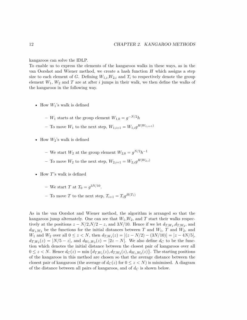
As in the van Oorshot and Wiener method, the algorithm is arranged so that thekangaroos jump alternately. One can see that W1,W2, and T start their walks respec-tively at the positions z −N/2,N/2− z, and 3N/10. Hence if we let dT,W1 ,dT,W2 , anddW1,W2 be the functions for the initial distances between T and W1, T and W2, andW1 and W2 over all 0 ≤ z < N , then dT,W1(z) =

∣∣(z −N/2)− (3N/10)∣∣ =

∣∣z − 4N/5∣∣,

dT,W2(z) =∣∣N/5 − z∣∣, and dW1,W2(z) =

∣∣2z − N ∣∣. We also define dC to be the func-tion which denotes the initial distance between the closest pair of kangaroos over all0 ≤ z < N . Hence dC(z) = min

{dT,W1(z), dT,W2(z), dW1,W2(z)

}. The starting positions

of the kangaroos in this method are chosen so that the average distance between theclosest pair of kangaroos (the average of dC(z) for 0 ≤ z < N) is minimised. A diagramof the distance between all pairs of kangaroos, and of dC is shown below.

2.4. THREE KANGAROO METHOD 13

The following table shows the the formula for dC , what C (the closest pair of kan-garoos) is, what B (the back kangaroo in C) is, and what F (the front kangaroo in C)is, across all 0 ≤ z < N .

dC(z) C B F0 ≤ z ≤ N/5 dT,W2(z) = N/5− z T and W2 T W2N/5 ≤ z ≤ 2N/5 dT,W2(z) = z −N/5 T and W2 W2 T

2N/5 ≤ z ≤ N/2 dW1,W2 = N − 2z W1 and W2 W1 W2N/2 ≤ z ≤ 3N/5 dW1,W2 = 2z −N W1 and W2 W2 W13N/5 ≤ z ≤ 4N/5 dT,W1(z) = 4N/5− z T and W1 W1 T

4N/5 ≤ z ≤ N/2 dT,W1(z) = z − 4N/5 T and W1 T W1

The expected number of steps until the IDLP is solved from a collision between theclosest pair can be analysed in the same way as the running time was analysed in thevan Oorshot and Weiner method.

• Stage 1. The period between when the kangaroos start their walks, and whenB catches up with F ’s starting position. The average of dC can easily be seen tobe N/10. Hence if we let m be the average step size used, the expected numberof steps for B to catch up to F ’s starting position is N/10m.

• Stage 2. The period between when stage 1 finishes, and when B lands on anelements of F ’s walk. The same analysis as was applied in the van Oorshot andWeiner method shows that the expected number of steps required in this stage ism.


• Stage 3. The period between when B lands on an element of F ’s path, and Blands on a distinguished point. In the three kangaroo method, the probabilityof a group element being distinguished is the same as it is in the van Oorshotand Wiener method, so the expected number of steps required in this stage is√N/c log(N).

If we make the pessimistic assumption that the IDLP will always be solved from acollision between the closest pair of kangaroos, we can expect the algorithm to requireN/10m+m+

√N/c log(N) steps to solve the IDLP. This expression is minimised when

m is taken to be√N/10. In this case, the algorithm requires

(2√

1/10 + o(1)))√N

steps to solve the IDLP. Since there are three kangaroos jumping at each step, theexpected number of group operations until the IDLP is solved is

(1.897 + o(1)

)√N

group operations.When Galbraith, Pollard and Ruprai considered the expected number of group oper-ations until the IDLP was solved from a collision between any pair of kangaroos (sonot just from a collision between the closest pair), they found through a complex anal-ysis, that the three kangaroo method has an expected average case running time of(1.818 + o(1)

)√N group operations. This is a huge improvement on the running time

of the van Oorshot and Weiner method.

2.5 Four Kangaroo Method

The Four kangaroo method is a very simple, but clever extension of the 3 kangaroomethod. As in the three kangaroo method, we start three kangaroos, T1, W1 andW2 atthe positions 3N/10, z−N/2, and N/2−z respectively. Here however, we add in one extratame kangaroo (T2), who starts his walk at 3N/10 + 1. One can see that the startingpositions of W1 and W2 have the same parity, while exactly one of T1 and T2’s startingpositions will have the same parity as W1 and W2’s starting positions. Therefore, if thestep sizes are defined to be even, then in any walk, both of the wild, and one of thetame kangaroos will be able to collide, while one of the tame kangaroos will be unableto collide with any other kangaroo. Therefore, the three kangaroos that can collide areeffectively simulating the three kangaroo method, except over an interval of half thesize. Hence, from the analysis of the three kangaroo method, the three kangaroos thatcan collide in this method require (1.818 + o(1))

√N/2 group operations to solve the

IDLP. However, since there is one ’useless’ kangaroo that requires just as many groupoperations as the three other useful kangaroos, the expected number of group operationsrequired to solve the IDLP by the four kangaroo method is (3 + 1)/3(1.818+o(1))

√N/2 =

2.6. CAN WE DO BETTER BY USING MORE KANGAROOS? 15

(1.714 + o(1))√N group operations.

2.6 Can we do better by using more kangaroos?

I now return to the main question this dissertation seeks to address. The answer to thisquestion is not clear through intuition, since there are arguments both for and againstusing more kangaroos.On the one hand, if one uses more kangaroos, we both increase the number of pairsof kangaroos that can collide, and we can make the kangaroos closer together. There-fore, by using more kangaroos, the number of steps until the first collision occurs willdecrease. However, by increasing the number of kangaroos, there will more kangaroosjumping at each step, so the number of group operations required at each step increases.

Chapter 3

Five Kangaroo Methods

This section will attempt to answer the two main questions of this dissertation (seeQuestion 1 and Question 2 in the introduction), by investigating kangaroo methodswhich use five kangaroos.

In this section, I will answer Question 2, and partially answer Question 1, by pre-senting a five kangaroo algorithm which requires on average

(1.737 + o(1)

)√N ±O(1)

group operations to solve the IDLP. To find a five kangaroo algorithm with this runningtime, I answered the following questions, in the order stated below.

• How should the walks of the kangaroos be defined in a 5 kangaroo algorithm?

• How many kangaroos of each type should be used?

• Where abouts should the kangaroos start their walks?

• What average step size should be used?

3.1 How the Walks of the Kangaroos are Defined

I will first investigate 5 kangaroo methods where a kangaroo’s walk can be defined inone of the same three ways as they were in the three and four kangaroo methods. This

17

18 CHAPTER 3. FIVE KANGAROO METHODS

means, that a kangaroo can either be of type Wild1,Wild2, or Tame, where the typesof kangaroos are defined in the following way.

• Wild1 Kangaroo - A kangaroo for which we express all elements of its walk inthe form gph, where p ∈ N.

• Wild2 Kangaroo - A kangaroo for which we express all elements of its walk inthe form grh−1, where r ∈ N.

• Tame Kangaroo - A kangaroo for which we express all elements of its walk inthe form gq, where q ∈ N.

As in the three and four kangaroo methods, there will be a hash function H whichassigns a step size to each x ∈ G. To walk the kangaroos around the group, if x isa kangaroos current group element, the group element it will jump to next will bexgH(x). As in all previous kangaroo methods, the algorithm will be arranged so thatthe kangaroos each take one jump during each step of the algorithm.

3.2 How many kangaroos of each type should be used?

If we let NW 1, NW 2 and NT respectively denote the number of wild1, wild2, andtame kangaroos used in any 5 kangaroo method. Then NW 1 + NW 2 + NT = 5. Thefollowing theorem will prove to be very useful in working out how many kangaroos ofeach type should be used, given this constraint.

Theorem 3.2. Let A be any 5 kangaroo algorithm, where the kangaroos can be of typeTame, Wild1, or Wild2. Then the expected number of group operations until the clos-est ’useful’ pair of kangaroos in A collides is no less than 10

√N

2NW 1NW 2+4NT (NW 1+NW 2)(A pair is called useful if the IDLP can be solved when the pair collides).

My proof of this requires Lemma 3.2.1, Lemma 3.2.2, Lemma 3.2.3, Lemma 3.2.4,and Lemma 3.2.5. Before stating and proving these lemmas, I will make the followingtwo important remarks.

• Remark 1. I showed in my description of the three kangaroo method how acollision between kangaroos of different types could solve the IDLP. On the other

3.2. HOW MANY KANGAROOS OF EACH TYPE SHOULD BE USED? 19

hand, we can gain no information about z from a collision between kangaroos ofthe same type. Hence a pair of kangaroos is ’useful’ if and only if it features twokangaroos of different types.

• Remark 2. In this section, for any choice of starting positions, I will let d (whered is a function of z) be the function that denotes the initial distance between theclosest useful pair of kangaroos across all 0 ≤ z < N . d is analogous to thefunction dC in the three kangaroo method, where for any z with 0 ≤ z < N ,d(z) will be defined to be the smallest distance between pairs of kangaroos ofdifferent types, at that particular z. Note that d(z) is completely determined bythe starting positions of the kangaroos.

Lemma 3.2.1. For any choice of starting positions in a 5 kangaroo algorithm, theminimal expected number of group operations until the closest useful pair collides is10√Ave(d(z)), where Ave(d(z)) is the average starting distance between the closest

useful pair of kangaroos over all instances of the IDLP (i.e. over all z ∈ N wherez ∈

[0, N

)=[0, N − 1

]).

Proof of Lemma 3.2.1. Let A be a 5 kangaroo algorithm that starts all kangaroos atsome specified choice of starting positions, and let m be the average step size used inA. Also let d(z) be defined as in remark 2. For each z with 0 ≤ z < N , using anargument very similar to that provided in section 2.2, the expected number of stepsuntil the closest useful pair collides for this specific z is d(z)/m+m. Since 5 kangaroosjump at each step, the expected number of group operations until the closest usefulpair collides for this z is 5(d(z)/m + m). Therefore, the expected average number ofgroup operations until the closest useful pair collides across all instances of the IDLP(i.e. across all z ∈ N with 0 ≤ z < N) is

1N

N−1∑z=0

5(d(z)m

+m

)

≈ 1N

∫ N−1

05(d(z)m

+m

)dz

= 5( 1

N

∫N−10 d(z)dzm

+m

)

≈ 5

1N

N−1∑z=0

d(z)

m+m

= 5(Ave(d(z))

m+m

).


Now simple differentiation shows that the m that minimises this is m =√Ave(d(z)).

Substituting in m =√Ave(d(z)) gives the required result.

Lemma 3.2.2. For each z, d(z) is either of the form |C1±z| or |C2±2z|, where C1 andC2 are constants independent of z. Furthermore, letting pg1 and pg2 respectively denotethe number of pairs with initial distance function of the form |C ± z|, and |C ± 2z|,pg1 = NT (NW 1 +NW 2), and pg2 = NW 1NW 2.

Proof of Lemma 3.2.2. Since a pair of kangaroos is useful if and only if it featurestwo kangaroos of different types, a pair is useful if and only if it is a tame/wild1, atame/wild2, or a wild1/wild2 pair (here a type1/type2 pair means a pair of kan-garoos featuring one kangaroo of type1, and another kangaroo of type2). Sinceall wild1,wild2 and tame kangaroos start their walks respectively at group ele-ments of the form gph,grh−1 and gq, for some p, q, r ∈ N, the starting positions ofall Wild1,Wild2 and Tame kangaroos will be of the forms p + z, r − z, and q re-spectively. Hence the initial distance functions between tame/wild1, tame/wild2,and wild1/wild2 pairs are respectively |p+ z − q|, |r − z + q|, and |p+ z − (r − z)|.Therefore, the distance function between all tame/wild1 and tame/wild2 pairs canbe expressed in the form |C1 ± z|, where C1 is independent of z. The number of suchpairs is NTNW 1 +NTNW 2. On the other hand, the initial distance function between awild1/wild2 pair can be expressed in the form |C2±2z|, where C2 is also independentof z. The number of such pairs is NW 1NW 2.

From the graph of dC in section 2.4, we can see that the function for the distancebetween the closest pair of kangaroos in the three kangaroo method is a sequence oftriangles. The same is generally true in five kangaroo methods. In lemma 3.2.3, I willshow that the area under the function d is minimised in five kangaroo methods whend is a sequence of triangles.

Lemma 3.2.3. Suppose d1,1, d1,2, d1,3, ..., dp1 and d2,1, d2,2, ..., d2,p2 are functions of z,defined on the interval [0, N), where for all i and j, d1,i(z) = |Ci ± z|, and d2,j(z) =|C2 ± 2z|, where Ci and Cj are constants. Let d(z) be defined such that ∀ 0 ≤ z < N ,d(z) = min {d1,1(z), d1,2(z), ..., d1,p1(z), d2,1(z), ..., d2,p2(z)}. Then assuming that wehave full control over the constants Ci and Cj, in every case where d is not a sequenceof triangles, the area under d can be decreased by making d into a sequence of triangles.This can be done by changing some of the constants Ci and Cj.

Proof. By d being a sequence of triangles, I mean that if we shade in the region beneathd, then the shaded figure is a sequence of triangles (see figure 3.2(a)). Now d is a


sequence of triangles if and only if S1,S2 and S3 hold, where S1 is the statement’d(0) = 0, or d(0) > 0 and d′(0) < 0’, S2 is the statement ’d(N−1) = 0, or d(N−1) > 0and d′(N−1) > 0’, and S3 is the statement ’for every z where the gradient of d changes,the sign of the gradient of d changes’. This is equivalent to the statement, ’for every zwhere the function which is smallest changes (from say da1,b1 to da2,b2), the gradientsof both da1,b1 and da2,b2 have opposite sign at z’.Hence if d is not a sequence of triangles, d must not satisfy at least one of the propertiesout of S1 (see figure 3.2(b)),S2 (see figure 3.2(c)), or S3 (see figures 3.2 (d) and (e)).


First consider the case where S1 doesn’t hold. Then d(0) > 0, and d′(0) > 0. LetdC0 be the function which is smallest out out of all{d1,1(z), d1,2(z), ..., d1,p1(z), d2,1(z), ..., d2,p2(z)} at z = 0. Hence dC0 = |C + gz|, whereC > 0, and g is 1 or 2, and d(z) = dC(z) for all z between 0 and p, for some p < N .If we change dC0 so that dC0 = |gz|, and define all other functions apart from dC0 inthe same way, then the area under d decreases by Cp over the region [0, p] (see figure3.2(f)), while the area under d over [p,N) will be no larger than it was before dC0(z)was redefined to be |gz|. Hence the area under d decreases by at least Cp over [0, N).Therefore, in every case where S1 doesn’t hold, we can decrease the area under d byredefining d so that S1 holds (Prop1).

Similarly, in the case where S2 doesn’t hold, d(N − 1) = C > 0 and d′(N − 1) < 0.If dCN is the function such that dCN (N − 1) = d(N − 1), then dCN (z) = |C − gz|,where C > g(N − 1) (since dCN (N − 1) > 0). Hence if we redefine dCN such thatdCN (z) = |g(N − 1)− gz|, if p is defined such that dCN (z) = d(z) ∀ p ≤ z < N (beforedCN (z) was defined to be |g(N − 1)− gz|), then the area under d decreases by at least


(N−1−p)(C−gN) (see figure 3.2(g)). Therefore, in every case where S2 doesn’t hold,we can decrease the area under d by redefining d so that S2 holds (Prop2).

Now consider the case where S3 doesn’t hold. Then there exists an x with 0 ≤ x < N ,and functions da1,b1 and da2,b2 such that the function which is smallest (so the functionwhich d equals) changes from da1,b1 to da2,b2 at x, and d′a1,b1

(x) and d′a2,b2(x) have the

same sign.In the case where d′a1,b1

(x) < 0 and d′a2,b2(x) < 0, (see figure 3.2(h)) d′a2,b2

(x) < d′a1,b1(x)

(since da2,b2(z) > da1,b1(z) for z < x with z ≈ x, and da2,b2(z) < da1,b1(z) for z > xwith z ≈ x. Hence da2,b2(x)′ = −2 and da1,b1(x)′ = −1. Therefore da2,b2(z) = |C2−2z|,and da1,b1(z) = |C1 − z| for some C1, C2 > 0. Now I will let [s, f ] be the regionsuch that for all z where s ≤ z ≤ f , d(z) = da1,b1(z) or d(z) = da2,b2(z), and h besuch that h = da1,b1(x) = da2,b2(x). Now if we fix da1,b1 (and all other functions in{d1,1(z), d1,2(z), ..., d1,p1(z), d2,1(z), ..., d2,p2(z)}), and allow da2,b2 to vary (by varyingthe constant C2), then assuming da1,b1 and da2,b2 intersect somewhere on the region[s, f ] when both d′a1,b1

< 0 and d′a2,b2< 0, then the area under d over the region [s, f ]

is determined purely by the height of this intersection point (Mathematically, it can beeasily shown that if we define H to be the height of the intersection point of da1,b1 andda2,b2 when da1,b1 and da2,b2 are decreasing, and A1s,f to be the area under da1,b1 over[s, f ], then the area under d over [s, f ] is A1s,f − 2H2/9). Now suppose we redefineda2,b2 so that da2,b2(z) = |C2− (x− s)− 2z| (as in figure 3.2(h)). Then da1,b1 and da2,b2

intersect with negative gradient when z = s, and the height of this intersection pointis h + (x − s). The following basic lemmas will be very useful for the remainder thisproof.

Lemma 3.2.3.1. If s > 0, d′(z) > 0 for z < s, with z ≈ s.

Proof. At any z, d′(z) is either −2,−1, 1 or 2. If d′(z) < 0 for z < s with z ≈ s, thensince da1,b1(z) = d(z) for z > s with z ≈ s, da1,b1 would still be the smallest function


for z < s, with z ≈ s. But this is a contradiction to [s, f ] being the region which eitherda1,b1 or da1,b1 are the smallest functions over.

Lemma 3.2.3.2. In the case where the intersection point of da1,b1 and da2,b2 whend′a1,b1

, d′a2,b2< 0 is when z = s, d satisfies S3 over [s, f ].

Proof. After da2,b2 is redefined, da1,b1 and da2,b2 are clearly still the smallest functionsover [s, f ]. Hence we only need to consider the intersection points of da1,b1 and da2,b2

to prove the lemma. By the nature of the functions da1,b1 and da2,b2 , da1,b1 and da2,b2

can have at most one intersection point when both d′a1,b1and d′a2,b2

have the same sign.Now da1,b1 and da2,b2 intersect when both have negative gradient when z = s. Hencethe only z where d’s gradient changes, but the sign of d’s gradient remains the sameover [s, f ], is when z = s. But Lemma 3.2.3.1 implies that the gradient of d changesfrom a positive to a negative value when z = s. Hence S3 is satisfied over [s, f ].

As a result, we can conclude x > s, since otherwise S3 would hold over [s, f ] whenda2,b2(z) was |C2 − 2z|. Hence the height of the intersection point of da1,b1 and da2,b2

when both d′a1,b1, d′a2,b2

< 0 is increased when da2,b2 is redefined, so the area under dover [s, f ] is decreased by redefining da2,b2 in such a way that d satisfies S3 over [s, f ].Since the value of d(z) doesn’t increase when da2,b2 is redefined for 0 ≤ z < s andf < z < N , the area under d over all other regions apart from [s, f ] does not increasewhen da2,b2 is redefined. Hence the area under d over [0, N) is decreased by redefiningd so that S3 is satisfied over [s, f ].A very similar argument can show that in the case where there exists a z such that thefunction which is smallest changes from dA1,B1 to dA2,B2 at z, and d′A1,B1

, d′A2,B2> 0,

then we can redefine dA2,B2 so that the area under d over [0, N) is decreased and S3is satisfied over [S, F ] (where S and F are defined such that d equals either dA1,B1 ordA2,B2 for all z with S ≤ z ≤ F ).Therefore, in every case where there exists z such that the gradient of d changes butkeeps the same sign at z, we can decrease the area under d over [0, N) by redefining oneof the functions in {d1,1(z), d1,2(z), ..., d1,p1(z), d2,1(z), ..., d2,p2(z)}, so that d satisfies S3over each of the intervals [s, f ] and [S, F ]. Hence, in such a case we can decrease thearea under d while making d satisfy S3 over [0, N) (Prop3).By combining Prop1,Prop2, and Prop3, we can conclude that in every case where dis not a sequence of triangles (so at least one of S1,S2 or S3 doesn’t hold for d), we candecrease the area under d by redefining d so that d is a sequence of triangles (so S1,S2and S3 all hold for d on [0, N)).


Figure 3.1: Diagram of the kind of situation being considered in lemma 3.2.4

In any five kangaroo method, we are given a set of functions of the same form asthose in lemma 3.2.3. To minimise the expected number of group operations until theclosest useful pair collides, we need to minimise the area under d, by choosing the Ci

and Cjs appropriately in functions of the form of lemma 3.2.3. Hence we may assumethat when the area under d is as small as possible, d will be a sequence of triangles.Therefore, since this theorem is stating a lower bound on the expected number ofgroup operations until the closest useful pair collides, for the purposes of the proof ofthis theorem, d can be assumed to be a sequence of triangles.The following lemma will be useful in finding how small the area under d can be, giventhat d can be assumed to be a sequence of triangles.

Lemma 3.2.4. Fix n,N ∈ N, and let the gradients G1,G2,...,Gn ∈ R \ {0} be fixed.Let R1,R2,...,Rn be such that Ri ≥ 0, ∑n

i=1Ri = N , and such that the sum of areasof triangles of base Ri and gradient Gi is minimised. Then all triangles have the sameheight.

Proof of Lemma 3.2.4. I will label the triangles such that the ith triangle (Ti) is thetriangle which has i − 1 triangles to the left of it. Gi can be considered to be thegradient of the slope of Ti, and Ri can be considered to be the size of the region whichTi occupies. Also let AT be the sum of area under these triangles. A diagram of thesituation is shown in Figure 3.1.

Then we haven∑

i=1Ri = N


andAT =

n∑i=1

|Gi|.R2i

2

In the arrangement where the heights of all the triangles are the same, for each 1 ≤ i <j < n, Ri/Rj = |Gj |/|Gi|. Suppose we change the ratio of Ri to Rj , so that the newRi is Ri + ε, and Rj becomes Rj − ε (note that ε can be greater than or less than 0).Then the area of Ti becomes (Gi(Ri + ε)2)/2 = (Gi(R2

i + 2Riε+ ε2))/2 while the areaof Tj becomes Gj(R2

j − 2Rjε+ ε2)/2. AT therefore changes by

|Gi|(Ri + ε)2

2 + |Gj |(Rj − ε)2

2 − |Gi|R2i

2 −|Gj |R2

j

2

= |Gi|R2i

2 +|Gj |R2

j

2 + |Gi|Riε− |Gj |Rjε−|Gi|R2

i

2 −|Gj |R2

j

2 + ε2

2 + ε2

2= |Gi|Riε− |Gj |Rjε+ ε2 = ε2 > 0

Therefore, adjusting the ratio of the size of any two regions away from that whichensures the height of the triangles is the same, always strictly increases the sum of thearea of the triangles. It follows that when the heights of all the triangles are equal, thesum of the area beneath these triangles is minimised.

Lemma 3.2.5. In the case where d is a sequence of triangles, each useful pair is eithernever the closest useful pair, or it is the closest useful pair over a single region.

Proof. By a useful pair (P ) being the closest useful pair only over a single region, Imean that there is a single interval [s, f ], with 0 ≤ s < f < N , such that P is theclosest useful pair for all z where s ≤ z ≤ f . This is in contrast to there being intervals[s1, f1], and [s2, f2], where 0 ≤ s1 < f1 < N , and f1 < s2 < f2 < N , such that P is theclosest useful pair for all z with s1 ≤ z ≤ f1, and s2 ≤ z ≤ f2, but P is not the closestuseful pair for all z where f1 < z < s2.The result of this lemma follows easily from the fact that if d is a sequence of triangles,then for every z where the closest useful pair changes (say from P1 to P2), the gradientsof the initial distance functions between P1, and P2 have opposite sign.

Proof of Theorem 3.2. The lemmas can now be used to prove the theorem. Firstly,label all useful pairs in any way from 1 to n, where n is the number of useful pairs of


kangaroos in A. Now since d can be assumed to be a a sequence of triangles, lemma3.2.5 implies that a useful pair is either never the closest useful pair, or there exists asingle region for which a useful pair is closest over. For each i, in the case where pairi is the closest useful pair over some region, let Ri denote the single region which pairi is the closest useful pair over, and Ris denote the size of Ri. In the case where pairi is never the closest useful pair, define Ris to be 0. Then ∑n

i=1Ris = N . Letting di

denote the distance function between pair i for each i, by Lemma 3.2.2, di(z) is of theform |C±giz|, where gi is 1 or 2, and C ∈ R. It is clear from the diagram in section 2.4that such functions feature at most two triangles, both of which have slopes of gradientwith an absolute value of gi. Hence di must feature at most two such triangles overRi. Now for every i, pair i is the closest useful pair over Ri, so d(z) = di(z) ∀z ∈ Ri.Therefore, d features at most two triangles over Ri, both of which have slopes thathave a gradient with an absolute value of gi. Therefore, if we let Tg1 and Tg2 denotethe number of triangles in d where the absolute values of their gradients are 1 and2 respectively, Tg1 ≤ 2pg1 = 2NT (NW 1 + NW 2) and Tg2 ≤ 2pg2 = 2NW 1NW 2. Nowby Lemma 3.2.4, for the area under d to be minimised, all triangles must have thesame height. This implies that all triangles with the same gradient in d must covera region of the same size. Defining RT1 and RT2 to denote the size of the regionscovered by each triangle of gradients 1 and 2 respectively, Lemma 3.2.4 also impliesthat RT1 = 2RT2 . Then since all triangles cover the domain of d, N = Tg1RT1 +Tg2RT2

≤ 2NT (NW 1 + NW 2)RT1 + 2NW 1NW 2RT2 = 4NT (NW 1 + NW 2)RT2 + 2NW 1NW 2RT2 .Hence RT2 ≥ N/(4NT (NW 1 +NW 2)+2NW 1NW 2). Now since all triangles in d have thesame height, the average of d over all z with 0 ≤ z < N is half the height of all triangles.Therefore, since the height of a triangle of gradient 2 is 2RT2 , RT2 gives the average ofd, which is the average distance between the closest useful pair. Then by Lemma 3.2.1,the expected number of group operations until the closest useful pair collides in the casewhere the area under d is minimised (and hence the average distance between the closestuseful pair is minimised) is 10

√RT2 ≥ 10

√N/(4NT (NW 1 +NW 2) + 2NW 1NW 2).

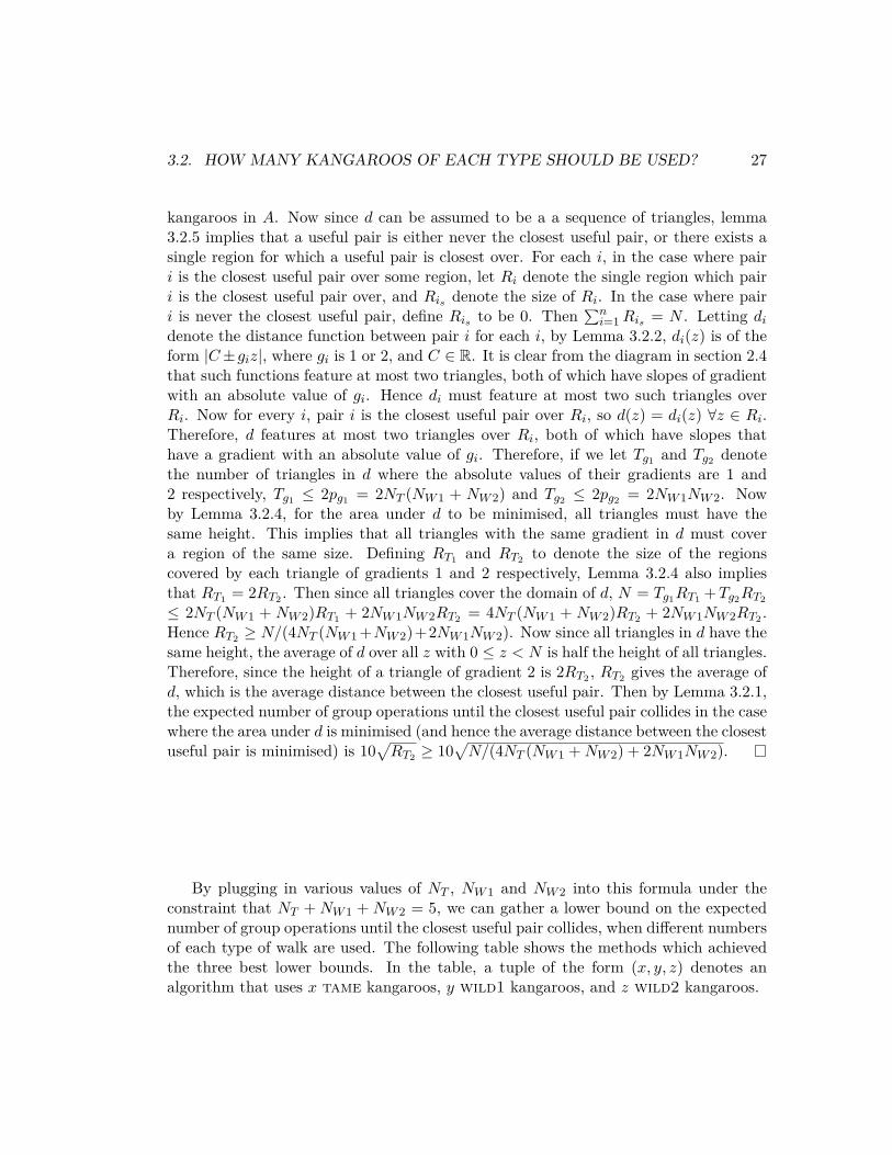
By plugging in various values of NT , NW 1 and NW 2 into this formula under theconstraint that NT + NW 1 + NW 2 = 5, we can gather a lower bound on the expectednumber of group operations until the closest useful pair collides, when different numbersof each type of walk are used. The following table shows the methods which achievedthe three best lower bounds. In the table, a tuple of the form (x, y, z) denotes analgorithm that uses x tame kangaroos, y wild1 kangaroos, and z wild2 kangaroos.


10√

N(4NT (NW 1+NW 2)+2NW 1NW 2) Number of walks of each type used

1.8898√N (2, 1, 2), (2, 2, 1)

1.9611√N (3, 1, 1)

2.0412√N (1, 2, 2), (2, 0, 3), (2, 3, 0),

(3, 0, 2), (3, 2, 0)

From this, it can be seen that a (2, 2, 1) 5 kangaroo method has the minimal lowerbound on the expected number of group operations until the closest useful pair collides,of 1.8898

√N group operations. A (2, 1, 2) method doesn’t need to be considered as a

separate case, since this is clearly equivalent to a (2, 2, 1) method. If one starts twowild1 kangaroos at h and g0.7124Nh, a wild2 kangaroo at g1.3562Nh−1, and two tamekangaroos at g0.9274N and g0.785N , the lower bound (2, 2, 1) method of 1.8898

√N group

operations is realised. The table shows that in any other 5 kangaroo method, the closestuseful pair can’t collide in less than 1.9611

√N group operations on average.

Since the closest useful pair of kangaroos is by far the most significant in determiningthe running time of any kangaroo algorithm (for instance, in the 3 kangaroo methodthe expected number of group operations until the closest useful pair collides could beas low as 1.8972

√N group operations, while the expected number of group operations

until any pair collides can only be as low as 1.818√N group operations), a method

that uses 2 tame, 2 wild1, and 1 wild2 kangaroos is most likely to be the optimal 5kangaroo method, out of all methods that only use tame,wild1, and wild2 kangaroos.

3.3 Where the Kangaroos should start their walks, andwhat average step size should be used?

Given that, in any 5 kangaroo method that uses only tame, wild1, and wild2 kan-garoos one should use 2 wild1, 1 wild2, and 2 tame kangaroos, the next question toconsider is where abouts the kangaroos should start their walks. In the analysis thatanswers this question, the question of what average step size to use will be answeredalso. I will now state some definitions and remarks that will be used throughout theremainder of this thesis.

• Remark 1: Firstly, I will redefine the IDLP to be to find z, given h = gzN ,when we’re given g and h, and that 0 ≤ z < 1.

3.3. DESIGNING A (2, 2, 1) KANGAROO ALGORITHM 29

• Remark 2: At this stage, I will place one constraint on the starting positionsof all kangaroos. This being, that all Wild1,Wild2, and Tame kangaroos willrespectively start their walks at positions of the form aN + zN , bN − zN , andcN , for universal constants a,b, and c, that are independent of the interval sizeN . This is the only constraint I will place on the starting positions at this stage.

• Remark 3: I will let Di,z denote the initial distance between the ith closestuseful pair of kangaroos for some specified z. It follows from Remark 2 thatDi,z = di,zN , for some di,z independent of N .

• Remark 4: The average step size m will be defined to be cm

√N , for some cm

independent of N .

• Remark 5: Si,z will be defined such that Si,z denotes the expected numberof steps the back kangaroo requires to catch up to the front kangaroo’s startingposition in the ith closest useful pair, for some specified z. It is clear that Si,z =dDi,z

m e. Since Di,z = di,zN , and m = cm

√N for some di,z, and cm which are

independent of N , we can say Si,z = dsi,z

√Ne for some si,z independent of N .

For the typical interval sizes over which one uses kangaroo methods to solve theIDLP (N > 230), this can be considered to be si,z

√N .

• Remark 6: Ci,z and ci,z will be defined such that Ci,z = ∑ij=1 Si,z, and

ci,z

√N = Ci,z. One can see from the definition of Si,z that ci,z is independent of

the interval size N .

I will answer the question that titles this section by first presenting a formula thatcan compute the running time of any (2,2,1) 5-kangaroo algorithm (see section 3.3.1),and then by showing how this formula can be used to find the best starting positionsand average step size to use (see section 3.3.2).


3.3.1 Formula for computing the running time of a (2,2,1)-5 kangarooalgorithm

Theorem 3.3.1. In any 5 kangaroo method which uses 2 tame, 1 wild2, and 2wild1 kangaroos, the expected number of group operations required to solve the IDLPis approximately5((∫ 1

0 czdz)

+ o(1))√

N +O(log(N)), where

cz =8∑

i=1

(e

(−isi,z+ci,z)cm (cm

i+ si,z)− e

−isi+1,z+ci,zcm (cm

i+ si+1,z)

).

Proof. Any 5 kangaroo method can be broken into the following 4 disjoint stages;

• Stage 1- The stage where the algorithm is initialised. This involves comput-ing the starting positions of the kangaroos, assigning a step size to each groupelement, and computing and storing the group elements which kangaroos aremultiplied by at each step (so computing gH(x) for each x in G).

• Stage 2- The period between when the kangaroos start their walks, and the firstcollision between a useful pair occurs.

• Stage 3- The period between when the first collision occurs, and when bothkangaroos have visited the same distinguished point.

• Stage 4- The stage where z is computed, using the information gained from auseful collision.

3.3.1.1 Number of group operations required in Stage 1

To find the starting positions of the kangaroos, we require one inversion (to find thestarting position of the kangaroo of type wild2), 3 multiplications (in finding thestarting positions of all wild kangaroos), and 5 exponentiations (one to find the start-ing position of each kangaroo). All of these operations are O(log(N)) in any group.As explained in [8], the step sizes can be assigned in O(log(N)) time also using a hashfunction. To pre-compute the group elements which kangaroos can be multiplied by ateach step, we need to compute gs, for each step size s that can be assigned to a group


element (this is the number of values which the function H can take). The numberof step sizes used in kangaroo methods is generally between 20 and 100. This wassuggested by Pollard in [8]. Applying less than a constant number (100) of exponen-tiation operations requires a constant number of group operations (so independent ofthe interval size).Summing together the number of group operations required by each part of Stage 1,we see that the number of group operations required in Stage 1 is O(log(N)).


To analyse the number of group operations required in stage 2, I will define Z(z) tobe a random variable on N such that Pr

(Z(z) = k

)denotes the probability that for

some specified z, the first collision occurs after k steps. From this, one can see thatE(Z(z)

)= ∑∞

k=0 kPr(Z(z) = k

), gives the expected number of steps until the first

collision occurs, at our specified z.

Important Remark

To compute E(Z(z)), I will compute the expected number of steps until the first usefulcollision occurs in the case where in every useful pair of kangaroos, the back kangarootakes the expected number of steps to catch up to the front kangaroos starting position,and make the assumption that this is proportional to the expected number of steps untilthe first useful collision occurs across all possible random walks. This assumption wasused implicitly in computing the running time of the three kangaroo method in [3],and is a necessary assumption to make, since calculating the expected number of stepsuntil the first useful collision occurs across all possible walks is extremely difficult.The following lemma will be useful in computing E(Z(z)).

Lemma 3.3.1. In the case where in every useful pair of kangaroos, the back kangarootakes the expected number of steps to catch up to the starting position of the front

kangaroo, for every k, Pr(Z(z) = k) =i∑

j=1

(ij

) 1mj e

−ik−i+Ci,z+j

m where i is the number of

pairs of kangaroos for which the back kangaroo has caught up to the front after k steps.

Proof. Let k ∈ N, and i be such that Si(z) ≤ k < Si+1(z). In the case where in everypair of kangaroos, the back kangaroo takes the expected number of steps to catch up


to the starting position of the front kangaroo, when Si(z) ≤ k < Si+1(z), there will beexactly i pairs where the back kangaroo will be walking over a region that has beentraversed by the front kangaroo (these will be the i closest useful pairs). Therefore,exactly i pairs can collide after k steps, for all Si(z) ≤ k < Si+1(z). In order for the firstcollision to occur after exactly k steps, we require that the i pairs that can collide avoideach other for the first k − 1 steps, and then on the kth step, j pairs collide for some jbetween 1 and i. I will define Ek,j to be the event that there are no collisions in the firstk − 1 steps, and then on the kth step, exactly j pairs collide. Since Ek,j and Ek,l are

disjoint events for j 6= l, we can conclude that Pr(Z(z) = k

)=

i∑j=1

P (Ek,j) (1). Now

Pr(Ek,j) can be computed as follows; In any instance where Ek,j occurs, we can definesetsX and Y such thatX is the set of all x where the xth closest useful pair of kangaroosdoesn’t collide in the first k−1) steps, but does collide on the kth step, and Y is the setof all y where the yth closest useful pair doesn’t collide in the first k steps. Now in Stage2 of the van Oorshot and Weiner method, I explained how at any step, the probabilitythat a pair collides once the back kangaroo has caught up to the path of the front is1/m. Hence for any x ∈ X, the probability that the back kangaroo in the xth closestuseful pair avoids the path of the front kangaroo for the first k − 1 steps, but lands onan element in the front kangaroos walk on the kth step is 1

m(1− 1m)k−Sx,z ≈ 1

me−k+Sx,z

m ,while for any y ∈ Y , the probability that the yth closest useful pair doesn’t collidein the first k steps is (1 − 1

m)k+1−Sy,z ≈ e−k−1+Sy,z

m . Now before any collisions havetaken place, the walks of any 2 pairs of kangaroos are independent of each other.Therefore, the probability that the pairs in X all first collide on the kth step, whileall the pairs in Y don’t collide in the first k steps is ∏x∈X

1me

−k+Sx,zm

∏y∈Y e

−k−1+Sy,zm

= 1mj e

−jk+∑

x∈XSx,z

m e−(i−j)k−(i−j)+

∑y∈Y

Sy,z

m = 1mj e

−ik−i+j+Ci,zm . Now since there are

(ij

)ways for j out of the i possible pairs to collide on the kth step, we obtain the formulaP (Ek,j) =

(ij

) 1mj e

−ik−i+j+Ci,zm . When substituting this result back into (1), we obtain

the required result of Pr(Z(z) = k) = ∑ij=1

(ij

) 1mj e

−ik−i+j+Ci,zm

I will now define pz to be the function such that pz(k) = kPr(Z(z) = k), for allk ∈ N . Hence E(Z(z)) = ∑∞

k=0 pz(k). Now in a 5 kangaroo method that uses 2 Tame,2 Wild1, and 1 Wild2 walks, there there are 8 pairs that can collide to yield a usefulcollision (4 Tame/Wild1 pairs, 2 Tame/Wild2 pairs, and 2 Wild1/Wild2 pairs).Hence for any k, the number of pairs where the back kangaroo has caught up to the


front kangaroos starting position can be anywhere between 0 and 8. Therefore,

pz(k) =

0 1 ≤ k < S1,z

kme

−k+C1,zm S1,z ≤ k < S2,z

k( 1me

−2k−1+C2,zm + 1

m2 e−2k+C2,z

m ) S2,z ≤ k < S3,z3∑

j=1k(3

j

) 1mj e

−3k−3+j+C3,zm S3,z ≤ k < S4,z

4∑j=1

k(4

j

) 1mj e

−4k−4+j+C4,zm S4,z ≤ k < S5,z

5∑j=1

k(5

j

) 1mj e

−5k−5+j+C5,zm S5,z ≤ k < S6,z

6∑j=1

k(6

j

) 1mj e

−6k−6+j+C6,zm S6,z ≤ k < S7,z

7∑j=1

k(7

j

) 1mj e

−7k−7+j+C7,zm S7,z ≤ k < S8,z

8∑j=1

k(8

j

) 1mj e

−8k−8+j+C8,zm S8,z ≤ k <∞

For the rest of this thesis, I will consider pz as a continuous function. The followingresult will be useful in computing E(Z(z)).

Theorem 3.3.1.1.∫∞

1 pz(k)dk −O(1) ≤ E(Z(z)) ≤∫∞

1 pz(k)dk +O(1).

Proof. The proof of this will use the following lemma.

Lemma 3.3.2. pz(k) is O(1) ∀k

Proof. Let 0 ≤ z < 1. Then ∀ k < S1,z, pz(k) = 0, while ∀ k ≥ S1,z, pz(k) =k∑i

j=1(i

j

) 1mj e

−ik−i+j+Ci,zm , for some 1 ≤ i ≤ 8. Hence for the purposes of the proof

of this lemma, we can assume k ≥ S1,z. I will state some facts that will make theargument of this proof flow more smoothly.

Fact 1: For k such that Si,z ≤ k < Si+1,z, e−ik−i+j+Ci,z

m ≤ 1.This holds because since k ≥ Si,z, ik ≥ iSi,z ≥

∑ij=1 Sj,z = Ci,z. Also, i ≥ j. Hence

−ik − i+ j + Ci,z ≤ 0, and e−ik−i+j+Ci,z

m ≤ 1.

Fact 2: No useful pair of kangaroos can start their walks further than a distanceof 6N apart on an interval of size N . Also, the average step size is at least 0.06697

√N .

Both of these facts will be explained in ’Remark regarding Lemma 3.3.2’ on Page 44.


Fact 3: The interval size can be assumed to be greater than 230. This wasexplained in the introduction, and can be assumed because one would typically usebaby-step giant-step algorithms to solve the IDLP on intervals of size smaller than 230.

I will show that pz(k) is O(1) for two separate cases.

Case 1: The case where S8,z ≤ m/8.First, consider the situation in this case where S1,z ≤ k ≤ m/8. Let i be such that Si,z ≤k < Si+1,z. Then by Fact 1, Fact 2, Fact 3, and the condition that k ≤ m/8, pz(k) =∑i

j=1(i

j

)k

mj e−ik−i+j+Ci,z

m ≤∑i

j=1(i

j

)k

mj ≤∑i

j=1(i

j

) m8

mj ≤∑i

j=1(i

j

) 18(0.06697

√230)j−1 , which

is clearly O(1).Now consider the case where k > m/8. Then since S8,z < m/8, k > S8,z. Hencepz(k) = ∑8

j=1 k(8

j

) 1mj e

−8k−8+j+C8,zm .

Hence dpz(k)dk =

(∑8j=1

(8j

) 1mj e

−8k−8+j+C8,zm

)(1− 8k

m

). This is less than 0 for k > m/8.

Hence ∀ k > m/8, pz(k) < pz(m/8). Since pz(m/8) is O(1), pz(k) is O(1) for k > m/8.

Case 2: The case where S8,z > m/8. First, consider the situation whereS1,z ≤ k ≤ S8,z. Let i be such that Si,z ≤ k < Si+1,z Now Fact 3 and Remark 5 (seePage 29) imply that S8,z ≤ 6N

0.06697√

N< 90

√N . Hence k < 90

√N . Therefore, pz(k) =∑i

j=1(i

j

)k

mj e−ik−i+j+Ci,z

m ≤∑i

j=1(i

j

)k

mj ≤∑i

j=1(i

j

)90√

Nmj ≤

∑ij=1

(ij

) 900.06697j(0.06697

√230)j−1

≤(8

1) 90

0.06697 +∑8j=2 o(1), which is O(1).

Now when k > S8,z, dpz(k)dk =

(∑8j=1

(8j

) 1mj e

−8k−8+j+C8,zm

)(1 − 8k

m ). Since k > S8,z >

m/8, dpz(k)dk < 0 ∀ k > S8,z. Therefore, pz(k) < pz(S8,z) ∀k > S8,z. Since pz(S8,z) is

O(1), pz(k) is O(1) ∀ k > S8,z.

I will now prove the theorem by approximating the sum of pz(k) over all k ∈ N to theintegral of pz(k), over each interval

[Si,z, Si+1,z

). On the interval [1, S1,z), pz(k) = 0,

so ∑Si,z−1k=1 pz(k) =

∫ S1,z

1 pz(k)dk (2). Hence for the rest of the proof I will considerpz(k) on intervals [Si,z, Si+1,z), where i ≥ 1. Now let pi,z be the function such thatpi,z(k) = k

∑ij=1

(ij

) 1mj e

−ik−i+j+Ci,zm (so pi,z(k) = pz(k) ⇐⇒ k ∈ [Si,z, Si+1,z)). Now by

differentiating pi,z, we obtain dpi,z

dk =(∑i

j=1(i

j

) 1mj e

−ik−i+j+Ci,zm

)(1− ki

m

). Hence pi,z


has a single turning point (at k = mi ). Since pz(k) = pi,z(k) for some i for every i ≥ 1,

on each interval [Si,z, Si+1,z), pz is either only decreasing, only increasing, or ∃ a t suchthat ∀ k < t, pz is increasing, and ∀ k > t, pz is decreasing.In the case where pz is only decreasing on an interval [Si,z, Si+1,z), by applying theintegral test for convergence, we can conclude that

∫ Si+1,z

Si,zpz(r)dr <∑Si+1,z−1

k=Si,zpz(k) <∫ Si+1,z

Si,zpz(r)dr + pz(Si,z) (3), while if pz is only increasing on [Si,z, Si+1,z),

∫ Si+1,z

Si,zpz(r)dr−

pz(Si,z) <∑Si+1,z−1k=Si,z

pz(k) <∫ Si+1,z

k=Si,zpz(r)dr (4).

Now consider pz on intervals of the form [Si,z, Si+1,z), where there exists a turningpoint t such that ∀ k < t, pz is increasing, while ∀ k > t, pz is decreasing (see figure3.3(a)). Let j be defined such that j = max{m ∈ N|n ≤ t− 1}. Then by applying theintegral for convergence test to the intervals [Si,z, j+ 1], and [j+ 2, Si+1,z], one can seethat ∑j+1

k=Si,zpz(k) >

∫ j+1k=Si,z

pz(r)dr and ∑Si+1,z−1k=j+2 pz(k) >

∫ Si+1,z

j+2 pz(r)dr. Therefore,∑Si+1,z−1Si,z

pz(k)+∫ j+2

j+1 pz(r)dr >∫ Si+1,z

Si,zpz(r)dr. Now

∫ j+2j+1 pz(r)dr = Ave{pz(r)|j+1 ≤

r ≤ j + 2}, which is O(1) since all pz(k) are O(1). Hence∫ Si+1,z

Si,zpz(r)dr − O(1) <∑Si+1,z−1

Si,zpz(k) (5).

Now the integral for convergence test, applied again to the intervals [Si,z, j + 1],and [j + 2, Si+1,z] implies that ∑j

k=Si,zpz(k) <

∫ j+1Si,z

pz(r)dr, and ∑Si+1,z−1k=j+3 pz(k) <∫ Si+1,z

j+2 pz(r)dr. Also, it is clear that pz(j + 1) + pz(j + 2) < pz(j + 1) + pz(j +2) +

∫ j+2j+1 pz(r)dr. Hence, ∑j

k=Si,zpz(k) + pz(j + 1) + pz(j + 2) + ∑Si+1,z−1

k=j+3 pz(k) <∫ j+1Si,z

pz(r)dr +∫ j+2

j+1 pz(r)dr +∫ Si+1,z

j+2 pz(r)dr. Therefore, since pz(j + 1) and pz(j + 2)are O(1), ∑Si+1,z−1

k=Si,zp(k) <

∫ Si+1,z

Si,zpz(r)dr +O(1) (6).


From (2),(3),(4), (5), and (6), we can see that for all intervals [Si,z, Si+1,z),

∫ Si+1,z

Si,z

pz(r)dr −O(1) <Si+1,z−1∑

Si,z

pz(k) <∫ Si+1,z

Si,z

pz(r)dr +O(1)

. Therefore, we obtain the required result of∫ ∞1

pz(k)dk −O(1) <∞∑

k=1pz(k) = E(Z(z)) <

∫ ∞1

pz(k)dk +O(1)

Hence for large interval sizes N ,∫∞

1 pz(k)dk approximates the expected number ofsteps until the first collision very well. The following lemma will make the computingof∫∞

1 pz(k)dk far more achievable.

Lemma 3.3.3. ∀i, j where 1 ≤ i ≤ 8, and j ≥ 2,∫ Si+1,z

Si,zk(i

j

) 1mj e

−ik+Ci,z−i+j

m is O(1).

Proof. The integral of k(i

j

) 1mj e

−ik+Ci,z−i+j

m with respect to k is

(ij

)(ik +m)e

−ik+Ci,z−i+j

m

i2mj−1

so∫ Si+1,z

Si,zk(i

j

) 1mj e

−ik+Ci,z−i+j

m dk is

(i

j

)(e−iSi,z+Ci,z−i+j

m (iSi,z +m)− e−iSi+1,z+Ci,z−i+j

m (iSi+1,z +m))

mj−1i2(7)

Now in the proof of Lemma 3.3.2, I showed that e−iSi,z+Ci,z−i+j

m ≤ 1. Hence (7) is lessthan (i

j)(Si,z+m)i2mj−1 . In the proof of the same lemma , I also showed that Si,z < 90

√N ,

and cm ≤ 0.06697√N . Hence (i

j)(Si,z+m)i2mj−1 < (90+0.06697)

√N

(0.06697√

N)j−1 , which is O(1) for j ≥ 2.

Therefore, from the formulas at the top of page 33, we see that∫ ∞1

pz(k)dk =8∑

i=1

∫ Si+1,z

Si,z

ik

me−ik+Ci,z−i+1

m +O(1) (8).


Now each∫ Si+1,z

Si,z

ikme

−ik+Ci,z−i+1m is

e−iSi,z+Ci,z−i+1

m (mi

+ Si,z)− e−iSi+1,z+Ci,z−i+1

m (mi

+ Si+1,z)

Substituting this into (8), we obtain∫ ∞

1pz(k)dk =

8∑i=1

(e−iSi,z+Ci,z−i+1

m (mi


m (mi

+ Si+1,z))

+O(1)

Now since Ci,z = ∑ij=1 Sj,z, Ci,z can be expressed as ci,z

√N , for some ci,z independent

of N . Hence8∑

i=1

(e−iSi,z+Ci,z−i+1

m (mi


m (mi

+ Si+1,z))

=8∑

i=1

(e

(−isi,z+ci,z)√

N−i+1cm√

N (cm

i+ si,z)

√N − e

(−isi+1,z+ci,z)√

N−i+1cm√

N (cm

i+ Si+1,z)

)√N

=8∑

i=1e−i+1

m

(e

(−isi,z+ci,z)cm (cm

i+ si,z)− e

−isi+1,z+ci,zcm (cm

i+ si+1,z)

)√N (9)

Now for the typical interval sizes over which one uses kangaroo methods to solve theIDLP (N > 230), e i+1

m is extremely close to 1. Hence we can safely ignore the e−i+1m term

in (9). I will state how large the approximation error due to ignoring this e−i+1m term

is when I present my final kangaroo algorithm in section 3.4. Therefore, if we define cz

to be∑8i=1

(e

(−isi,z+ci,z)cm ( cm

i + si,z)− e−isi+1,z+ci,z

cm ( cmi + si+1,z)

), we have

∫∞1 pz(k)dk−

O(1) = cz

√N . Using the result from Theorem 3.3.1.1, we can conclude that

E(Z(z)) = cz

√N ±O(1) (10)

Hence the expected number of steps until the first collision over all instances of theIDLP (i.e. over all z with 0 ≤ z < N) is

E(Z) = c√N ±O(1) (11)

where c = Ave{cz|0 ≤ z < 1} =∫ 1

0 czdz. Now since at each step, each of the 5 kangaroosmake one jump, the expected number of group operations until the first collision occursacross all z is

5(∫ 1

0czdz

)±O(1) (12)



From the analysis provided in [3], if one sets the probability that a group element isdistinguished to be c log(N)

√N, for some constant c > 0, the expected number of

group operations required in stage 3 is√N/c log(N) = o(1)

√N .

3.3.1.4 Number of Group operations required in Stage 4

The kangaroos used in a 2 tame, 2 wild1, and 1 wild2 kangaroo method are of thesame type as those used in the three kangaroo method. I explained how one may findz from a collision between any of these types of kangaroos when I described the threekangaroo method. In any case, at most 3 addition or subtraction operations modulo|g|, while in the case where a Wild1 and a Wild2 kangaroo collides, we are requiredto find 2−1 (mod |g|). Hence the number of group operations required in this stage isO(1).

Now by summing the number of group operations required in stages 1,2,3 and 4,we obtain the required result that the expected number of group operations requiredto solve the IDLP by any 2 tame, 2 wild1, and 1 wild2 kangaroo method, is approx-imately 5

((∫ 10 czdz

)+ o(1)

)√N +O(log(N)).

3.3.2 Finding a good assignment of starting positions, and averagestep size

In this subsection, I will use the formula presented in Theorem 3.3.1 to find the bestchoice of starting positions and average step size that I could possibly find.The process I will use to do this will be to first state how the formula of Theorem 3.3.1can be used compute the running time of an algorithm with particular starting positionsand average step size (see Algorithm 1), and then to iterate through various possiblestarting positions and average step sizes, to find which one minimises the running time.For this purpose, I will define a,b,c,t1, and t2 to be universal constants independent ofthe interval size N , such that on an interval of size N , the 2 Wild1 kangaroos starttheir walks at the positions aN + zN and cN + zN , the Wild2 kangaroo starts hiswalk at bN − zN , and the 2 Tame kangaroos start their walks at t1 and t2.

One can see from the formula of Theorem 3.3.1, that finding the running time of


any 5 kangaroo method requires finding∫ 1

0 czdz. Now calculating cz at any z requiresfinding si,z ∀ i with 1 ≤ i ≤ 8. The most rigorous approach to finding the averageof cz would be to find a formula for each si,z across all z, and to plug this into theformula for cz, and then integrate this across all z. Finding a direct formula for eachsi,z that holds for all possible choices for the starting positions and the average step sizeproved to be too difficult. I therefore proposed the following simulation based approachfor computing

∫ 10 czdz. This is how the computeaveragecz function of Algorithm 1

computes∫ 1

0 czdz.At a particular z, si,z can be computed by finding the starting positions of all kangarooson an interval of size N = 1 (this means computing aN+zN = a+z, b−z, c+z, t1 andt2), and then finding the distances between all useful pairs when the kangaroos startat these positions. By then ranking these distances in the manner done in line 5 ofAlgorithm 1, one can find Di,z for each i between 1 and 8, for an interval of size N = 1.One can then find si,z using Di,z/m = di,zN/cm

√N = si,z

√N = si,z. Following this,

we can compute all ci,z, using ci,z = ∑ij=1 sj,z. Hence we have all the information we

need to compute cz. By finding the average of cz for a large number of evenly spacedz in [0, 1) (so for instance, computing cz for all z in {z|z = 10−pk, k ∈ N, 0 ≤ z < 1},with p ≥ 3), we can approximate

∫ 10 czdz. The pseudocode for the matlab® function

to compute cz is shown in Algorithm 1.

Algorithm 1 Function for finding the average of cz

1: function computeaveragecz(a,b,c,t1,t2,cm,p)2: z ←− 03: sumofcz ←− 04: while z < 1 do5: distancesarray ← sort({

|(a+ z)− t1| , |(b− z)− t1| , |(c+ z)− t1| , |(a+ z)− t2||(b− z)− t2| , |(c+ z)− t2| , |(a+ z)− (b− z)| , |(c+ z)− (b− z)|

})

6: for i← 1 to 8 do7: si,z ← distancesarray[i]/cm

8: ci,z ←∑i

j=1 sj,z

9: cz ←∑8

i=1

(e

(−isi,z+ci,z)cm ( cm

i + si,z)− e−isi+1,z+ci,z

cm ( cmi + si+1,z)

)10: sumofcz ← sumofcz + cz

11: z ← z + 10−p

12: return sumofcz/(10p)

Therefore, if we let Opt denote the output of this function on some specified combi-nation of starting positions and average step size (i.e. values of a,b,c,t1,t2 and cm), thenfrom (11), the expected number of steps until the first collision occurs for this combi-


nation is Opt

√N ± O(1) (13). Also, from the formula of theorem 3.3.1, the expected

number of group operations required to solve the IDLP for our specified combinationof starting positions and average step size is approximately (5Opt + o(1))

√N ± O(1)

(14). I will state how large the error of this approximation is when I present my fivekangaroo algorithm in section 3.4.

Therefore, if we let aopt,bopt,copt,t1opt ,t2opt , and cmopt respectively denote the bestvalues for a,b,c,t1,t2 and cm, then aopt,bopt,copt,t1opt ,t2opt , and cmopt are the values ofa,b,c,t1,t2 and cm for which the output of the computeaveragecz function is smallest.

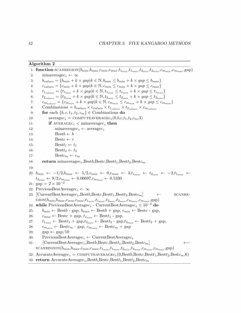
This fact gives rise the to the following algorithm for finding good values fora,b,c,t1,t2, and cm. The pseudocode for this algorithm is shown in Algorithm 2. Theidea of the algorithm was to start with a range of values for which the optimal val-ues of a,b,c,t1,t2, and cm lay in. These ranges would be encapsulated in the variablesamin,amax,bmin,bmax,cmin,cmax,t1min ,t1max ,t2min ,t2max ,cmmin and cmmax , so we wouldhave amin ≤ aopt ≤ amax, bmin ≤ bopt ≤ bmax, cmin ≤ copt ≤ cmax, t1min ≤ t1opt ≤ t1max ,t2min ≤ t2opt ≤ t2max . I was unable to prove a range of values for which aopt,bopt,copt,t1opt ,t2opt , and cmopt were guaranteed to lie in, but in (A),(B),(C),(D) and (E)(which can be found below), I state and justify some ranges for which aopt,bopt,copt,t1opt ,t2opt , and cmopt are likely to lie in. Using the scanregion function, I wouldthen find good values for b,c,t1,t2 and cm (by (A), a can be fixed at 0) by computingaveragecz for evenly spaced (separated by the amount defined by the variable ’gap’ inAlgorithm 2) values of b,c,t1,t2, and cm, between the ranges defined by the variablesbmin,bmax,cmin,cmax,t1min ,t1max ,t2min ,t2max ,cmmin and cmmax (see lines 3-10). The vari-ables Bestb,Bestc, Bestt1, Bestt2, and Bestcm would represent the values of b,c,t1,t2and cm for which averagecz was smallest, across all combinations for which averagecz

was computed for (this is carried out in lines 9-18).We could then find better values for b,c,t1,t2 and cm than Bestb, Bestc, Bestt1, Bestt2,and Bestcm, by running the scanregion function on values of b,c,t1,t2 and cm in asmaller region centred around Bestb, Bestc, Bestt1, Bestt2, and Bestcm (see lines 25-28),that are separated by a smaller gap (see line 29). By repeating this process multipletimes (see lines 24-31), we could keep finding better and better values for b,c,t1,t2 andcm. Eventually however, the interval for which the scanregion function was called onwould shrink to be zero in size. At this point, the the improvements in the best valuesfor b,c,t1,t2 and cm between iterations would become negligible. Line 24 determineswhen this occurs.The algorithm then computes Averagecz to a higher degree of accuracy for the optimalvalues of b,c,t1,t2 and cm (see line 32). It does this by setting the variable p in theComputeaveragecz function to be 6 (p was set to 3 the main loop (see line 10), due


to reasons relating to the practicality of the running time of Algorithm 2).

Estimates of initial bounds for the optimal values of a,b,c,t1,t2 and cm

(A). aopt = 0

(B). −12 = bmin ≤ bopt ≤ bmax = 5

2

(C). 0 = cmin ≤ copt ≤ cmax = 3, and c ≥ a

(D). −2 = t1min = t2min ≤ t1opt ≤ t2opt ≤ t1max = t2max = 92

(E). 0.06697 ≤ cmopt ≤ 0.5330

Justification of (A). Suppose we start our kangaroos walks at N(d + z),N(b + d −z),N(c + d + z),N(t1 + d), and N(t2 + d), where d ∈ R. Then for all z, one can seethat the starting distances between all pairs of kangaroos is the same in this case aswhen the kangaroos start their walks at N(0 + z),N(b− z),N(c+ z),t1N and t2N (thatis, if we subtract dN from all kangaroos starting positions). Hence if we use the sameaverage step size in both cases, the running time in both algorithms will be the same.Hence for any algorithm where a > 0, there exists an algorithm where a = 0 which hasthe same running time. Hence we only need to check the case where a = 0, so we canclaim that aopt = 0

Justification of (B). The bound presented here is very loose. If b−a > 2.5, or b < a−0.5then ∀ z, on an interval of size N , the initial distance between the kangaroos that starttheir walks at a+ z and b− z is at least N/2 (when z = 0, |(a+ z)− (−0.5− z)| = 0.5,and when z = 1, |(a + z) − (2.5 − z)| = 0.5). Now in the three kangaroo method, onan interval of size N , the furthest the initial distance between the closest useful pairof kangaroos could be across all z was N/5 (this occurred when z was 0, 2N/5, 3N/5and N). Now in a good five kangaroo method, since there are more kangaroos (than ina three kangaroo method), we can expect to the furthest initial distance between theclosest useful pair of kangaroos across all z to be smaller than N/5. Hence if a pair ofkangaroos in a five kangaroo method always starts their walks at least distance N/2apart, such a pair is highly unlikely to ever collide before the closest useful pair collides,at any z, and will therefore be extremely unlikely to ever be the pair which collidesfirst. In a good 5 kangaroo algorithm, it would be natural to suppose that every usefulpair of kangaroos can be the pair whose collision leads to the solving of the IDLP (i.e.


Algorithm 21: function scanregion(bmin,bmax,cmin,cmax,t1min ,t1max ,t2min ,t2max ,cmmin ,cmmax ,gap)2: minaveragecz ←∞3: bvalues = {bmin + k × gap|k ∈ N, bmin ≤ bmin + k × gap ≤ bmax}4: cvalues = {cmin + k × gap|k ∈ N, cmin ≤ cmin + k × gap ≤ cmax}5: t1values

= {t1min + k × gap|k ∈ N, t1min ≤ t1min + k × gap ≤ t1max}6: t2values

= {t2min + k × gap|k ∈ N, t2min ≤ t2min + k × gap ≤ t2max}7: cmvalues

= {cmmin + k × gap|k ∈ N, cmmin ≤ cmmin + k × gap ≤ cmmax}8: Combinations = bvalues × cvalues × t1values

× t2values× cmvalues

9: for each {b, c, t1, t2, cm} ∈ Combinations do10: averagecz = computeaveragecz(0,b,c,t1,t2,cm,3)11: if averagecz < minaveragecz then12: minaveragecz ← averagecz

13: Bestb← b14: Bestc← c15: Bestt1 ← t116: Bestt2 ← t217: Bestcm ← cm

18: return minaveragecz,Bestb,Bestc,Bestt1,Bestt2,Bestcm

19:20: bmin ← −1/2,bmax ← 5/2,cmin ← 0,cmax ← 3,t1min ← t2min ← −2,t1max ←

t2max ← 9/2,cmmin ← 0.06697,cmmax ← 0.533021: gap = 2× 10−2

22: PreviousBestAveragecz ←∞23:

[CurrentBestAveragecz,Bestb,Bestc,Bestt1,Bestt2,Bestcm

]← scanre-

gion(bmin,bmax,cmin,cmax,t1min ,t1max ,t2min ,t2max ,cmmin ,cmmax ,gap)24: while PreviousBestAveragecz - CurrentBestAveragecz ≤ 10−4 do25: bmin ← Bestb - gap, bmax ← Bestb + gap, cmin ← Bestc - gap,26: cmax ← Bestc + gap, t1min ← Bestt1 - gap,27: t1max ← Bestt1 + gap,t2min ← Bestt2 - gap,t2max ← Bestt2 + gap,28: cmmin ← Bestcm - gap, cmmax ← Bestcm + gap29: gap ← gap/1030: PreviousBestAveragecz ← CurrentBestAveragecz

31:[CurrentBestAveragecz,Bestb,Bestc,Bestt1,Bestt2,Bestcm

]←−

scanregion(bmin,bmax,cmin,cmax,t1min ,t1max ,t2min ,t2max ,cmmin ,cmmax ,gap)32: AccurateAveragecz = computeaveragecz(0,Bestb,Bestc,Bestt1,Bestt2,Bestcm,6)33: return AccurateAveragecz,Bestb,Bestc,Bestt1,Bestt2,Bestcm


can collide first), at some z. Hence it is not desirable for there to be a useful pair whichalways starts its walk at least distance of 0.5N apart on an interval of size N .

Justification of (C). Firstly let W1,1 denote the kangaroo that starts its walk at N(a+z), and W1,2 denote the kangaroo that starts at N(c + z). Since these kangaroos areof the same types (they’re both Wild1 kangaroos), if we fix c,t1,t2 and cm, then analgorithm where W1, 1 starts at a + z and W1,2 starts at c + z, has the same runningtime as an algorithm where W1,1 starts at c + z and W1,2 starts at a + z, since the 2Wild1 walks that start at the same positions in both cases. Hence copt ≥ aopt = 0.Now copt ≤ 3, since if c > 3, then on an interval of size N , the distance between thekangaroos that start their walks at N(c+ z) and N(b− z) can never be less than N/2.I gave evidence that this was not desirable in my justification of (B). Hence we maysuppose that 0 ≤ copt ≤ 3.

Justification of (D). Firstly, we only need to check values where t2opt ≥ t1opt , becauseone can show in a similar way to the one shown in proving copt ≥ aopt, that for every casewhere t2 < t1, there exists an algorithm with the same running time where t1 < t2.Now −2 ≤ t1, t2 ≤ 9/2, since if t1 and t2 are outside this range, then the startingdistance between any wild kangaroo and any of the tame kangaroos on an interval ofsize N is at least N/2.

Justification of (E). I stated in Section 3.2 that by starting the kangaroos walks at h,g0.7124Nh, g1.3562Nh−1,g0.9274N and g0.785N , the lower bound for the expected numberof group operations until the closest useful pair collides (ECP ) of 1.8898

√N group

operations could be realised. Using Lemma 3.2.1 in the proof of Theorem 3.2, theaverage distance between the closest useful pair across all z when ECP = 1.8898

√N

group operations is 0.0357N . In the proof of the same lemma, I also showed thatECP = 5(Ave(d(z))/m + m), where Ave(d(z)) denotes the average distance betweenthe closest useful pair of kangaroos over all z. Hence Ave(d(z)) ≥ 0.0357N in any 5kangaroo algorithm. Therefore, ECP ≥ 5(0.0357N/cm

√N + cm

√N). One could suppose

that there must be some bound B, such that if the expected number of group operationsfor the closest useful pair to collide in some algorithm is larger than B, then thisalgorithm could have no chance of being the optimal 5 kangaroo algorithm. A very loosebound on B is 3

√N . For ECP ≤ 3

√N , we require 5(0.0357N/cm

√N+cm

√N) ≤ 3

√N .


For this to occur, cm must range between 0.06697, and 0.5330. Hence we can suppose0.06697 ≤ cmopt ≤ 0.5330.

Remark regarding Lemma 3.3.2

Lemma 3.3.2 required an upper bound on how far apart a useful pair of kangarooscan be when they start their walks. When t2 is 4.5, b = −0.5, and zN = N − 1, theinitial distance between the Wild2 kangaroo that starts its walk at (b− z)N , and theTame kangaroo that starts his walk at t2N , is 6N − 1 < 6N . In any method wherethe variables a, b, c, t1 and t2 are within the bounds presented in (A),(B),(C) and (D),no useful pair of kangaroos can start their walks further apart than this.The same lemma also required a lower bound on the average step size used. (E) showsthat one lower bound is 0.06697

√N .

Results

When I ran Algorithm 2 in matlab®, the values for a,b,c,t1,t2 and cm which werereturned had a = 0, b = 1.3578, c = 0.7158, t1 = 0.7930, t2 = 0.9220, and cm = 0.3118.Algorithm 2 computed averagecz to be 0.3474 in this case.Using the result of (14) (see the top of page 40), we see that in an algorithm wherea,b,c,t1,t2 and cm are defined to be these values requires on average

(5 × 0.3474 +

o(1))√N ±O(1) =

(1.737 + o(1)

)√N ±O(1) group operations to solve the IDLP.

Formula (13) also implies that the expected number of steps until the first collisionwill be 0.3474

√N ±O(1) steps (15).

3.4 Five Kangaroo Method

I now present my five kangaroo algorithm.If we are solving the IDLP on an interval of size N over a group G, and we start thewalks of five kangaroos at the group elements h, g1.3578Nh−1, g0.7158Nh, g0.922N , andg0.793N , and use an average step size of 0.3118

√N , and let the kangaroos walk around

the group G in the manner defined in section 3.1, then we can expect to solve the IDLP

3.4. FIVE KANGAROO METHOD 45

in on average(1.737 + o(1)

)√N ±O(1) group operations.

Note that 1.3578N ,0.7158N ,0.922N , and 0.793N might not be integers, so in practice,the kangaroos would start their walks at h, gbh−1, gch, gt1 , and gt2 , where b,c,t1, andt2 are respectively the closest integers to 1.3578N ,0.7158N ,0.922N , and 0.793N .There are two main factors which have not been accounted for in this calculation of therunning time. The first is eluded to in the remark, stated just before Lemma 3.3.1. Thisbeing, that I calculate the expected running time in the instance where for every z, theback kangaroo takes the expected number of steps to catch up to the starting positionof the front kangaroo in every useful pair of kangaroos, and make the assumption thatthis is proportional to the average expected running time across all possible walks thatthe kangaroos can make. I was unable to find a bound for how much the approximationerror would be increased by because of this assumption. However, in [3], Galbraith,Pollard and Ruprai make the same assumption in computing the running time of thethree and four kangaroo methods. They were also unable to find a bound for muchthe approximation error would be increased by because of this assumption. However,when Galbraith, Pollard and Ruprai gathered experimental results to test how welltheir heuristic estimates worked in practice, they found that their experimental resultsmatched their estimated results well [3]. Hence I can assume the magnitude of theapproximation error is not affected too badly as a result of this assumption.The other factor that wasn’t accounted for in my calculation of the running time, washow I ignore the e−i+1

m term in (9) (see page 37). Since m = 0.3118√N in my 5

kangaroo algorithm, and in practice, one would typically use kangaroo methods onintervals of size at least 230, the multiplicative factor of the approximation error dueto this is has a lower bound of e−i+1

m ≥ e−7

0.3118√

N ≥ e7

0.3118√

230 ≥ 1− (7× 10−4), and anupper bound of 1.This five kangaroo algorithm is therefore a huge improvement on the previously optimalfive kangaroo method of Galbraith, Pollard, and Ruprai, which required at least 2

√N

group operations to solve the IDLP on average. This algorithm also beats the runningtime of the three kangaroo method, so it therefore answers one of the main questionsof this dissertation. This being, ’Are five kangaroos worse than three?’.

Chapter 4

Seven Kangaroo Method

Using the same idea that was applied by Galbraith, Pollard and Ruprai in [3] in extend-ing the three kangaroo method to the four kangaroo method, the five kangaroo methodcan be extended to give a seven kangaroo method, with slightly improved running time.If we are solving the IDLP on an interval of size N , let A,B, and C respectively bethe closest even integers to 0,1.3578N , and 0.7158N , and let T1 and T2 be the closestintegers to 0.422N , and 0.793N . Suppose we start the walks of 7 kangaroos at thegroup elements h, gBh−1, gCh, gT1 , gT1+1, gT2 , and gT2+1. Then we are effectivelystarting two Wild1 kangaroos at positions z, and C + z, one Wild2 kangaroo at theposition B − z, and four Tame kangaroos at the positions T1, T1 + 1, T2 and T2 + 1.Now z, B − z and C + z are either all odd, or all even. Hence all Wild1 and Wild2kangaroos start their walks an even distance apart. Also, exactly one of T1 and T1 + 1,and exactly one of T2 and T2 + 1 are of the same parity as z, B − z and C + z. I willlet T1useful

and T2usefuldenote the Tame kangaroos whose starting positions are of the

same parity as the starting positions of the Wild1 and Wild2 kangaroos, and T1useless

and T2uselessdenote the two other tame kangaroos.

Now suppose we make all step sizes even. Then T1uselessand T2useless

will be unable tocollide with any other kangaroo, excluding themselves. However, T1useful

,T2useful, and

all Wild1 and Wild2 kangaroos are able to collide, and are all starting their walks atat almost the exact same positions as the five kangaroos do in the five kangaroo methodof section 3.4. Hence, assuming the algorithm is arranged so that all kangaroos jumpone after the other in some specified order, then these 5 kangaroos (T1useful

,T2useful, the

Wild2 kangaroo, and the two Wild1 kangaroos) are effectively performing the fivekangaroo method of section 3.4, except over an interval of size N/2, since the fact that

47

48 CHAPTER 4. SEVEN KANGAROO METHOD

all step sizes are even means that only every second group element is being consideredin this method. Hence from the statement of (15) (see the results section on page 44),the expected number of steps until the first collision occurs is

(0.3474

√N/2 ± O(1)

)= 0.2456

√N ± O(1) steps. However, since there are now 7 kangaroos jumping at

each step, the expected number of group operations until the first collision occurs is7×0.2456

√N±O(1) = 1.7195

√N±O(1) group operations. By defining the probability

that a point is distinguished in the same way as it was in the five kangaroo method,we can conclude that the seven kangaroo method presented here requires on averagean estimated

(1.7195 + o(1)


As I have already stated, currently the fastest kangaroo method is the four kangaroomethod. This has an estimated average running time of (1.714 + o(1))

√N group op-

erations. Therefore, the seven kangaroo method presented here is very close to beingthe optimal kangaroo method.

Chapter 5

Conclusion

The main results of this thesis were the following.

• Result 1: The presentation of a five kangaroo algorithm which requires on av-erage

(1.737 + o(1)


• Result 2: The presentation of a seven kangaroo method that requires on average(1.7195 + o(1)


For clarity, I will restate the main questions that this thesis attempted to answerhere also.

• Question 1: Can we improve kangaroo methods by using larger numbers ofkangaroos?

• Question 2: Are 5 kangaroos worse than three?

Before this dissertation, the four kangaroo method of Galbraith, Pollard, and Ruprai[3] was by the far the best kangaroo algorithm. This algorithm has an estimated av-erage running time of

(1.714 + o(1)

)√N group operations. It was unknown whether

we could beat the running time of the four kangaroo method by using more than fourkangaroos. The fastest algorithm that used more than four kangaroos was far slower

49

50 CHAPTER 5. CONCLUSION

than the four kangaroo method, requiring on average at least 2√N group operations

to solve the IDLP.The five and seven kangaroo algorithms presented in this report are a significant im-provement in kangaroo methods that use more than four kangaroos. Even though therunning time of the methods presented in this thesis did not beat the running time ofthe four kangaroo method, they came very close to doing so. Therefore, even thoughthe main question of this dissertation (Question 1) still remains unanswered, we cannow have more confidence that kangaroo methods can be improved by using more thanfour kangaroos.Question 2 was also answered in this thesis, since the estimated average running timeof the five kangaroo method presented in section 3.4 (

(1.737 + o(1)

)√N ±O(1) group

operations) beat the estimated average running time of the three kangaroo method of[3] (

(1.818 + o(1)

)√N group operations).

References

[1] Boneh D, Goh E, Nissim K. Evaluating 2-DNF formulas on ciphertexts. Theory ofcryptography: Springer; 2005. p. 325-341.

[2] Galbraith SD, Ruprai RS. Using equivalence classes to accelerate solving the dis-crete logarithm problem in a short interval. Public Key Cryptography–PKC 2010:Springer; 2010. p. 368-383.

[3] Galbraith SD, Pollard JM, Ruprai RS. Computing discrete logarithms in an interval.Mathematics of Computation 2013;82(282):1181-1195.

[4] Gaudry P, Schost É. A low-memory parallel version of Matsuo, Chao, and Tsujii’salgorithm. Algorithmic number theory: Springer; 2004. p. 208-222.

[5] Gopalakrishnan K, Thériault N, Yao CZ. Solving discrete logarithms from partialknowledge of the key. Progress in Cryptology–INDOCRYPT 2007: Springer; 2007.p. 224-237.

[6] Lim CH, Lee PJ. A key recovery attack on discrete log-based schemes using a primeorder subgroup. Advances in Cryptology—CRYPTO’97: Springer; 1997. p. 249-263.

[7] Pohlig SC, Hellman ME. An improved algorithm for computing logarithms over andits cryptographic significance (corresp.). Information Theory, IEEE Transactions on1978;24(1):106-110.

[8] Pollard JM. Kangaroos, monopoly and discrete logarithms. J Cryptol2000;13(4):437-447.

[9] Pollard JM. Monte Carlo methods for index computation (mod p). Mathematics ofcomputation 1978;32(143):918-924.

[10] Shanks D. Class number, a theory of factorization, and genera. Proc. Symp. PureMath; 1971.

51

52 REFERENCES

[11] Teske E. Square-root algorithms for the discrete logarithm problem (a survey). InPublic Key Cryptography and Computational Number Theory, Walter de Gruyter:Citeseer; 2001.

[12] Van Oorschot PC, Wiener MJ. Parallel collision search with cryptanalytic appli-cations. J Cryptol 1999;12(1):1-28.

[13] Van Oorschot PC, Wiener MJ. Parallel collision search with application to hashfunctions and discrete logarithms. Proceedings of the 2nd ACM Conference on Com-puter and communications security: ACM; 1994.

Kangaroo Methods for Solving the Interval Discrete ...sgal018/AFhons.pdf · Kangaroo Methods for...

Documents

Transcript of Kangaroo Methods for Solving the Interval Discrete ...sgal018/AFhons.pdf · Kangaroo Methods for...