
Kalman-based schemes for mobile nodes localization in · PDF fileKalman-based schemes for...
88
Kalman-based schemes for mobile nodes localization in ad-hoc networks Esquemas de localizaci´ on de nodos m´oviles en redes ad-hoc basados en filtros de Kalman Juli´ an Alberto Pati˜ no Murillo Universidad Nacional de Colombia Facultad de Ingenier´ ıa y Arquitectura Departamento de Ingenier´ ıa El´ ectrica,Electr´onicayComputaci´on Manizales, Colombia 2011
Transcript of Kalman-based schemes for mobile nodes localization in · PDF fileKalman-based schemes for...

Kalman-based schemes for mobilenodes localization in ad-hoc networks
Esquemas de localizacion de nodos moviles en redesad-hoc basados en filtros de Kalman
Julian Alberto Patino Murillo
Universidad Nacional de Colombia
Facultad de Ingenierıa y Arquitectura
Departamento de Ingenierıa Electrica, Electronica y Computacion
Manizales, Colombia
2011


Kalman-based schemes for mobilenodes localization in ad-hoc networksEsquemas de localizacion de nodos moviles en redes
ad-hoc basados en filtros de Kalman
Julian Alberto Patino Murillo
Tesis o trabajo de grado presentada(o) como requisito parcial para optar al tıtulo de:
Magister en Ingenierıa - Automatizacion Industrial
Director(a):
Ph.D. Jairo Jose Espinosa Oviedo
Lınea de Investigacion:
Matematicas Avanzadas para el Control y los Sistemas Dinamicos
Grupo de Investigacion:
GAUNAL
Universidad Nacional de Colombia
Facultad de Ingenierıa y Arquitectura
Departamento de Ingenierıa Electrica, Electronica y Computacion
Manizales, Colombia
2011


Dedicated to
To my beloved ones, my Mother Aracelly and my Brother Alejo,
because they are the strength that makes me get up every day and
their support is always there for me...
To my Granny Consuelo, who taught me to have faith and
to know that good things happens when you believe...and by
extension to all the Murillo’s Family...
And to Marley (just be patient, Honey!)
Dedicatoria
A mis seres mas queridos, mi Madre Aracelly y mi hermano Alejo,
porque ellos son la fuerza que me hace levantarme cada dıa y su
apoyo siempre esta disponible para mı...
A mi mamita Consuelo, quien me enseno a tener fe y a saber que
cosas buenas pasan cuando creemos...y por extension a toda la
familia Murillo...
Y a Marley (teneme un poquito de paciencia!)


Acknowledgements
First, I would like to thank Professor Jairo Espinosa for taking a chance on me without
knowing, and because he still sees in me the capabilities for giving much more.
To the Gaunal bunch (Alejo, Jose, Jose David, Pablo, Felipe, Richard, Cesar, Camilo, Juan
Esteban, Andrea) for all the laughs, and for all the help and encouragement during the last
three years and counting.
To my people from Control Engineering 2001 promotion (Sau, Cata, Camilo, Juan David,
Juan David F., Juan Diego, Sara, Marce, Diana R., Diana P., Juan Pablo, Leyton, Esteban,
Saul, Monica, Laura) because you always will be my friends. Your success makes me happy,
and forces me to become a better human being each day just to keep up with you. Love you
guys!
To my big family, because of their unwavering support that makes me persevere day after day.
To Colciencias and Facultad de Minas of the Universidad Nacional de Colombia for providing
the funding for my studies through the programs Convocatoria 463 de 2008 and Convocato-
ria 496 de 2009 from ”Programa Nacional de Jovenes investigadores e innovadores”during
the last two years.
To Marley, for her love and support.
And, finally, to my mother and brother for their unconditional love and their believe that I
can accomplish anything I purpose myself to do.


ix
Resumen
Esta tesis enfrenta el problema de la determinacion de la posicion de nodos moviles en
redes inalambricas ad hoc, con base en las mediciones del indicador de potencia de la senal
recibida (RSSI). Las caracterısticas de movilidad de los nodos se modelan a traves de un
sistema no lineal representado por un modelo de Giro Coordinado (CTM). La localizacion
de la posicion de los nodos se lleva a cabo mediante multilateracion integrada con diferentes
esquemas para refinar la estimacion basados en las tecnicas de Kalman: FIltro Extendido
de Kalman (EKF); Filtro de Kalman Unscented”(UKF); y dos Filtros de Multiples Modelos
Interactuantes (IMM), los cuales consisten en un conjunto de Filtros de Kalman Extendi-
dos (IMM-EKF) y un banco de Filtros de Kalman Unscented”(IMM-UKF). Se alcanza a
estimacion de los estados del modelo de movilidad, los cuales comprenden la posicion, la
velocidad y, eln algunos casos, el parametro de Tasa de Giro del nodo objetivo movil. El de-
sempeno de los diferentes esquemas basados en Kalman se compara mediante el seguimiento
de dos trayectorias a traves de simulaciones Monte Carlo.
Palabras clave: Redes ad hoc, Localizacion de nodos, Seguimiento de trayectorias, Esti-
macion, Filtros de Kalman, Filtro de Kalman Extendido, Filto de Kalman Unscented”,
Multiples Modelos Interactuantes.
Abstract
This thesis addresses the problem of position localization of mobile nodes in ad hoc wireless
networks based on received signal strength indicator (RSSI) measurements. Node mobility is
modelled as a non-linear system driven a Coordinated Turn Model (CTM). Self-localization
of mobile nodes is performed via multilateration integrated with a different collection of
Kalman based schemes for estimation refinement: Extended Kalman Filter (EKF); Unscent-
ed Kalman Filter (UKF); an two Interacting Multiple Model Filter consisting of a bank of
Extended Kalman Filters (IMM-EKF) and Unscented Kalman Filters (IMM-UKF). Esti-
mation of the mobility state, which comprises the position, speed and, in some cases, the
Turn Rate parameter of the mobile node is accomplished. The performance of the Kalman
based filters is compared through the tracking of two different trajectories by Monte Carlo
simulation.
Keywords: Ad hoc networks, Node Localization, Trajectory Tracking, Kalman Filter,
Extended Kalman Filter, Unscented Kalman Filter, Interacting Multiple Model

Contents
Acknowledgements VII
Abstract IX
List of Abbreviations XIV
1. Introduction 1
1.1. Mobile nodes self-localization in ad hoc networks . . . . . . . . . . . . . . . . 1
1.2. Motivation . . . . . . . . . . . . . . . . . . . . . . . . . . . . . . . . . . . . . 2
1.3. Objectives . . . . . . . . . . . . . . . . . . . . . . . . . . . . . . . . . . . . . 2
1.4. Chapter by chapter overview . . . . . . . . . . . . . . . . . . . . . . . . . . . 3
2. Ad Hoc Wireless Sensor Networks 4
2.1. What is a Wireless Ad hoc Network? . . . . . . . . . . . . . . . . . . . . . . 4
2.1.1. Types of Wireless Ad hoc Networks . . . . . . . . . . . . . . . . . . . 5
2.2. What is an Ad Hoc Wireless Sensor Network? . . . . . . . . . . . . . . . . . 5
2.2.1. Applications of Ad Hoc Wireless Sensor Networks . . . . . . . . . . . 6
2.2.2. Properties of Ad Hoc Wireless Sensor Networks . . . . . . . . . . . . 9
2.2.3. Challenges in the Design of Ad Hoc Wireless Sensor Networks . . . . 9
3. Self Localization in Mobile Ad Hoc Networks 13
3.1. Localization . . . . . . . . . . . . . . . . . . . . . . . . . . . . . . . . . . . . 13
3.2. Technical Challenges . . . . . . . . . . . . . . . . . . . . . . . . . . . . . . . 14
3.2.1. Network Topology . . . . . . . . . . . . . . . . . . . . . . . . . . . . 15
3.2.2. Estimating the Distance Between Two Nodes . . . . . . . . . . . . . 16
3.3. A brief literature survey about ad-hoc localization schemes . . . . . . . . . . 18
3.3.1. Ranging . . . . . . . . . . . . . . . . . . . . . . . . . . . . . . . . . . 19
3.3.2. Positioning . . . . . . . . . . . . . . . . . . . . . . . . . . . . . . . . 19
3.3.3. Refinement . . . . . . . . . . . . . . . . . . . . . . . . . . . . . . . . 23
4. Mobility and observation models for mobile node localization 26
4.1. Localization of mobile nodes . . . . . . . . . . . . . . . . . . . . . . . . . . . 26
4.2. Discrete-Time State Space Models . . . . . . . . . . . . . . . . . . . . . . . . 27
4.2.1. Linear state space estimation . . . . . . . . . . . . . . . . . . . . . . 29

Contents xi
4.2.2. Discretization of continuous-time linear time-invariant systems . . . . 29
4.3. Mobility Models . . . . . . . . . . . . . . . . . . . . . . . . . . . . . . . . . . 30
4.3.1. CWPA Model . . . . . . . . . . . . . . . . . . . . . . . . . . . . . . . 30
4.3.2. CWPV Model . . . . . . . . . . . . . . . . . . . . . . . . . . . . . . . 31
4.3.3. Position Model . . . . . . . . . . . . . . . . . . . . . . . . . . . . . . 32
4.3.4. Coordinated Turn Model . . . . . . . . . . . . . . . . . . . . . . . . . 32
4.4. Measurement Model . . . . . . . . . . . . . . . . . . . . . . . . . . . . . . . 33
5. The application of Kalman-based schemes to localization 34
5.1. Theoretical tools . . . . . . . . . . . . . . . . . . . . . . . . . . . . . . . . . 34
5.1.1. Lateration . . . . . . . . . . . . . . . . . . . . . . . . . . . . . . . . . 34
5.1.2. Kalman Filter . . . . . . . . . . . . . . . . . . . . . . . . . . . . . . . 34
5.1.3. Kalman Filter for Tracking Problems . . . . . . . . . . . . . . . . . . 37
5.1.4. Kalman Filters for Non-linear State Estimation . . . . . . . . . . . . 37
5.1.5. Extended Kalman Filter (EKF) . . . . . . . . . . . . . . . . . . . . . 37
5.1.6. Unscented Kalman Filter . . . . . . . . . . . . . . . . . . . . . . . . . 40
5.1.7. Multiple Model Systems . . . . . . . . . . . . . . . . . . . . . . . . . 43
5.2. Algorithm Description . . . . . . . . . . . . . . . . . . . . . . . . . . . . . . 45
5.3. Hypothesis Test: ANOVA Analysis . . . . . . . . . . . . . . . . . . . . . . . 47
6. Simulation results 50
6.1. Wiener Process Models Performance Comparison . . . . . . . . . . . . . . . 50
6.1.1. Simulation Description . . . . . . . . . . . . . . . . . . . . . . . . . . 50
6.1.2. Discussion of Results . . . . . . . . . . . . . . . . . . . . . . . . . . . 52
6.2. Target Tracking . . . . . . . . . . . . . . . . . . . . . . . . . . . . . . . . . . 56
6.2.1. Simulation Description . . . . . . . . . . . . . . . . . . . . . . . . . . 56
6.2.2. Results for trajectory 1 . . . . . . . . . . . . . . . . . . . . . . . . . . 58
6.2.3. Results for trajectory 2 . . . . . . . . . . . . . . . . . . . . . . . . . . 62
7. Conclusions and future work 67
7.1. Conclusions . . . . . . . . . . . . . . . . . . . . . . . . . . . . . . . . . . . . 67
7.2. Future Work . . . . . . . . . . . . . . . . . . . . . . . . . . . . . . . . . . . . 68
Bibliography 69

List of Tables
5-1. IMM-EKF Localization Algorithm Procedure . . . . . . . . . . . . . . . . . 46
5-2. IMM-UKF Localization Algorithm Procedure . . . . . . . . . . . . . . . . . 46
5-3. EKF Localization Algorithm Procedure . . . . . . . . . . . . . . . . . . . . . 47
5-4. UKF Localization Algorithm Procedure . . . . . . . . . . . . . . . . . . . . . 47
6-1. Simulation parameters for Wiener Process Models Performance Comparison 51
6-2. Average of the error metrics for trajectory estimation . . . . . . . . . . . . . 53
6-3. Simulation parameters for Target Tracking . . . . . . . . . . . . . . . . . . . 58
6-4. Description of Trajectory 1 . . . . . . . . . . . . . . . . . . . . . . . . . . . . 58
6-5. Average of RMSE values for Trajectory 1 . . . . . . . . . . . . . . . . . . . . 59
6-6. Description of Trajectory 2 . . . . . . . . . . . . . . . . . . . . . . . . . . . . 62
6-7. Average of RMSE values for Trajectory 2 . . . . . . . . . . . . . . . . . . . . 63

List of Figures
2-1. Wireless Networks Classification . . . . . . . . . . . . . . . . . . . . . . . . . 4
4-1. Ad-hoc sensor network architecture . . . . . . . . . . . . . . . . . . . . . . . 27
5-1. The lateration process . . . . . . . . . . . . . . . . . . . . . . . . . . . . . . 35
6-1. Simulation testbed for trajectory estimation . . . . . . . . . . . . . . . . . . 51
6-2. Best estimation results with different q values . . . . . . . . . . . . . . . . . 54
6-3. Average Distance Error with the different values of q . . . . . . . . . . . . . 55
6-4. ANOVA analysis with q = 50 . . . . . . . . . . . . . . . . . . . . . . . . . . 55
6-5. ANOVA analysis with q = 0,5 . . . . . . . . . . . . . . . . . . . . . . . . . . 56
6-6. Representation in 2D of Target trajectory 1. . . . . . . . . . . . . . . . . . . 59
6-7. A sample of position estimation results for trajectory 1 . . . . . . . . . . . . 60
6-9. MSE of velocity estimation for trajectory 1 . . . . . . . . . . . . . . . . . . . 60
6-8. MSE of position estimation for trajectory 1 . . . . . . . . . . . . . . . . . . . 61
6-10.ANOVA analysis of position estimation for trajectory 1 . . . . . . . . . . . . 62
6-11.Representation in 2D of Target trajectory 2. . . . . . . . . . . . . . . . . . . 63
6-12.A sample of position estimation results for trajectory 2 . . . . . . . . . . . . 64
6-13.MSE of position estimation for trajectory 2 . . . . . . . . . . . . . . . . . . . 64
6-14.MSE of velocity estimation for trajectory 2 . . . . . . . . . . . . . . . . . . . 65
6-15.ANOVA analysis of position estimation for trajectory 2 . . . . . . . . . . . . 66

List of Abbreviations
Abbreviation Term
AhLoS Ad Hoc Localization System
ANOV A Analysis of Variance
AoA Angle of Arrival
APS Ad Hoc Positioning System
BER Bit Error Rate
CWPA Continuous Wiener Process Acceleration (PV A)
CWPV Continuous Wiener Process Velocity (PV )
DE Distance Error
EKF Extended Kalman Filter
GPS Global Positioning System
IMM Interacting Multiple Model
KF Kalman Filter
MANET Mobile Ad Hoc Network
MDS −MAP Multi-Dimensional Scaling
MinMax Minimum-Maximum Algorithm
MSE Mean Squared Error
P Position Model
RMSE Root Mean Squared Error
RSS Received Signal Strength
RSSI Received Signal Strength Indicator
ToA Time of Arrival
TDoA Time Difference of Arrival
UKF Unscented Kalman Filter
WMN Wireless Mesh Networks
WSN Wireless Sensor Networks

1 Introduction
1.1. Mobile nodes self-localization in ad hoc networks
The movement patterns of mobile users play an important role in performance analysis of
wireless computer and communication networks in which nodes may move freely within an
area. The structure of ad hoc wireless networks can change dynamically over time; this fact
complicates the network control and management tasks. It is very important for this kind of
network to localize the node positions and movement [17] [64] [45] as the transmitter range
is generally fairly small with respect to the size of the area. Self localization [35] involves
the combination of absolute location information (e.g., obtained from a Global Positioning
System (GPS)) with relative distance information (e.g. distance measurements between sen-
sors) over regions of the network. It is also desirable to minimize the amount of inter-sensor
communications.
There are many methods for self-localization, one class is based on signal measurements
and their statistical models (see, e.g., the surveys [17] [45] [35]). These methods rely up-
on the signal time-of-arrivals, time difference of arrivals, angle-of-arrivals or received signal
strengths and they vary in their complexity and accuracy. In this thesis we consider the
self-localization of mobile nodes in wireless ad hoc networks using received signal strength
indicator (RSSI) measurements. Node mobility is modelled with a linear dynamic model,
with multiple acceleration modes, which are driven by a discrete Markov process. Due to the
fact that the control process of the mobile node is unknown and we have multiple acceleration
levels, the Interacting Multiple Model approach [5] is suitable for the considered problem.
We implemented it in combination with an Extended Kalman Filter (requires linearization
of the non-linear measurement equations) and an Unscented Kalman Filter (affords avoid-
ing linearization of the highly non-linear measurement equations). The IMM Kalman-based
filters are compared with EKF and UKF algorithms for mobile nodes self-localization.
Previous approaches to mobile nodes localization depend on the type of the ad hoc network
[35]: indoor or outdoor. In the indoor sensor network the localization can be performed with
beacons (fixed or moving) or it can be beacon free. In outdoor applications GPS systems are
mainly used. Many localisation techniques rely on Kalman Filtering [36] [59] [37] and Monte
Carlo techniques [20], including and knowledge of the connectivity between the nodes. Some
works [45] consider the case when nodes can communicate among each other which is not

2 1 Introduction
always possible because communications are energy-consuming.
1.2. Motivation
The absence of a fixed infrastructure in wireless ad hoc networks make them suitable for use
in emergency situations as well as for low cost commercial communication systems. How-
ever, the flexibility of the highly dynamic ad hoc networks complicates important control
and management tasks such as routing, flow control, and power management. For example,
traffic routes change over time, subject to the movement of the mobile nodes. The effective-
ness of any routing algorithm depends heavily on the accuracy and timelines of the available
network topology information. In ad hoc networks, knowledge of the network topology can
be inferred from the mobility of the nodes. The absence of a fixed infrastructure in wireless
ad hoc networks make them suitable for use in several applications of target tracking as well
as for low cost commercial communication systems.
Although different algorithms for self-localization and tracking have been proposed in the
literature, this is an open and active research area, where many questions from theoretical
and practical point of view remain unsolved. The difficulties are coming from the changeable
network topology, the need of communications between the nodes under limited resources
(energy, bandwidth), noisy data and the challenge of overcoming losses.
1.3. Objectives
General Objective
The aim of this thesis is to present a performance comparison of a collection of Kalman based
tools capable of target tracking in ad-hoc networks by solving one or both target motion and
measurement uncertainties.
Specific Objectives
The development of tracking algorithms for ad-hoc networks based on Kalman filters
and IMM techniques using distance measurements and lateration.
The implementation of a simulation scheme for the evaluation of the developed local-
ization algorithms.
The selection of a performance metric for the comparison of the simulation results of
the studied methods.

1.4 Chapter by chapter overview 3
1.4. Chapter by chapter overview
This thesis is organized in 5 chapters. A brief description of each chapter is given as follows.
Chapter 2: This chapter presents an introduction of the Ad Hoc Wireless Sensor
Networks, with a brief definition and an illustration of its properties, applications and
the current design challenges.
Chapter 3: This chapter presents an overview of the problem of self-localization of
nodes in ad hoc networks, and it shows the stages of the localization process. Also,
it describes the state of the art of the localization and tracking solutions for ad hoc
networks found in literature.
Chapter 4: This chapter describes the mobility models used to represent the dynamics
of the mobile target, and it also shows the measurement model for extracting position
information from the RSSI data over the ad hoc network.
Chapter 5: This chapter presents a detailed description of the theoretical tools used
to develop the localization algorithms, such as lateration and Kalman Filter and its
derivatives (EKF - UKF). We also introduce the Interacting Multiple Models tools
for the estimation of the target trajectory. Later, some algorithms for localization and
tracking using Kalman Filter in ad hoc networks are presented.
Chapter 6: In this chapter, the simulation results of the studied methods are present-
ed.
Conclusions: This dissertation finishes with some concluding remarks and outlines
posible future work areas on this matter.

2 Ad Hoc Wireless Sensor Networks
There is a major difference between wireless and wired networks: the former makes the
transmission of the information through air and the latter through physical cables. Therefore,
the main difference between wired and wireless is the infrastructure. At the wired networks:
wires, switches, hubs and all the other communication means are responsible for transporting
the information while at wireless networks signals and waves propagate through the air.
Figure 2-1 presents a wireless networks classification according to [30]. As it is the subject
of this thesis, the following sections introduce the characteristics of the Ad Hoc Wireless
Sensor Networks.
Figure 2-1: Wireless Networks Classification
2.1. What is a Wireless Ad hoc Network?
A wireless ad hoc network is a decentralized wireless network with a dynamical structure
changing over time, which complicates the network control and management tasks. Data
can be forwarded from any node to any other node through zero, one or more intermediate
nodes. Other characteristics are:
Multi-hop routing is a common feature in ad hoc networks: data from a source to
destination may go through certain intermediate nodes.

2.2 What is an Ad Hoc Wireless Sensor Network? 5
Each node can send data, receive data and also act as a router forwarding data for
peers.
Wireless cellular networks need a fixed infrastructure where an access point manages com-
munication among nodes. In contrast, a wireless ad hoc network requires minimal prior
configuration and can be quickly deployed: the devices self-organize among themselves to
form a network on the fly. The emphasis here is on the ad hoc character of these kinds
of networks; it implies that network deployment and configuration happens with no need
of previous preparation, and assumes no existing infrastructure in the area of deployment.
The dynamic aspect of these kind of networks constitutes its most interesting and more
challenging characteristic.
2.1.1. Types of Wireless Ad hoc Networks
Ad hoc Network (MANET)
A MANET is a self-organizing wireless network of mobile devices. The topology of the
network (arrangement of the devices) changes dynamically with time. An example of this
kind of networks are the Vehicular Ad hoc Networks(VANET) [63]. A type of MANET that
is fast gaining wide research focus, VANETs are used for communication among vehicles
(equipped with wireless devices) and between vehicles and roadside equipment.
Wireless Mesh Networks (WMN)
A WMN is an ad hoc network where all nodes are generally static and mobility is not an
issue. A WMN is composed of mesh clients (laptops, cell phones and etc.) and mesh routers
that forward traffic towards and from the mesh clients to the gateways that connect to the
Internet. The mesh topology provides multiple paths from the source to the destination
and helps in quick reconfiguration of paths when an existing path fails. The WMN nodes
are normally not resource constrained. An example of a WMN could be a mesh formed by
placing wireless relaying equipment on the top of houses [2].
Wireless Sensor Networks (WSN)
Being the main subject of this thesis, this kind of ad hoc networks will be reviewed in the
next section with more detail.
2.2. What is an Ad Hoc Wireless Sensor Network?
Generally speaking, an ad hoc wireless sensor network consists of a large number of self-
sufficient nodes with sensing capabilities. The nodes can perform simple computations and

6 2 Ad Hoc Wireless Sensor Networks
communicate with each other through a self-deployed and self-healing multihop communica-
tion network [1]. The sensors are distributed over a region to cooperatively monitor physical
or environmental conditions (such as temperature, pressure, pollutant concentration, forest
fire, etc.) at different locations and report the data to a central base station (commonly
called sink).
Each node in a sensor network is typically equipped with one or more sensors; a radio
transceiver for communication; a micro-controller for computation and decision making and
a battery. The lifetime of each individual sensor may not as significant but lifetime of the
entire network may be an important performance metric.
2.2.1. Applications of Ad Hoc Wireless Sensor Networks
The claim of wireless sensor network proponents is that this technological vision will facili-
tate many existing application areas and bring into existence entirely new ones. This claim
depends on many factors, but a couple of the envisioned application scenarios shall be high-
lighted. Apart from the need to build cheap, simple to program and network, potentially
long-lasting sensor nodes; a crucial and primary ingredient for developing actual applica-
tions is the actual sensing and actuating capabilities of a sensor node. For many physical
parameters, appropriate sensor technology exists that can be integrated in a node of a WSN.
Some of the few popular ones are temperature, humidity, visual and infra-red light (from
simple luminance to cameras), acoustic, vibration (e.g. for detecting seismic disturbances),
pressure, chemical sensors (for gases of different types or to judge soil composition), me-
chanical stress, magnetic sensors (to detect passing vehicles), potentially even radar [13].
But even more sophisticated sensing capabilities are conceivable.
The rest of this section presents a number of applications of ad hoc wireless sensor networks
found in the literature.
Environmental applications
Although there are some other techniques to monitor environmental conditions, random dis-
tribution and self organization of WSNs make them suitable for environmental monitoring.
WSNs can be used to control the environment, for example, with respect to chemical pol-
lutants: a possible application are garbage dump sites. Another example is the surveillance
of the marine ground floor; an understanding of its erosion processes is important for the
construction of offshore wind farms. Closely related to environmental control is the use of
WSNs to gain an understanding of the number of plant and animal species that live in a giv-
en habitat (biodiversity mapping). The main advantages of WSNs here are the long-term,
unattended, wire-free operation of sensors close to the objects that have to be observed;
since sensors can be made small enough to be unobtrusive, they only negligibly disturb the

2.2 What is an Ad Hoc Wireless Sensor Network? 7
observed animals and plants. Often, a large number of sensors is required with rather high
requirements regarding lifetime. Some of the specific ongoing study cases over this field are:
Planetary exploration [3]
Geophysical monitoring [61]
Habitat monitoring [33]
Bio-complexity mapping [24]
Oceanography [7]
Transportation Systems
Cars equipped with sensors can form local communication networks sharing information on
weather and road conditions, plan efficiently chosen routes, avoid traffic and identify their
position in areas where GPS signals are unavailable [9].
Structural Monitoring
Sensors are placed on structures to detect structural weaknesses, the presence of hazardous
materials and, their reaction to extreme weather and physical phenomena [29]. These sensors
can form local communication networks and forward the information they gather to central
points where suitable simulation models can then decide on the need for structural changes
and help prevent accidents.
Medical and Physiological Monitoring
Wireless sensors can be used in hospitals to efficiently locate doctors and patients and when
attached to medications, they can minimize the danger of issuing the wrong medication
to patients [28]. Small sensors, each with different sensing capabilities, can be attached to
different parts of the body of a patient to measure physiological signatures, detect infections
and automatically regulate her medication or alert doctors [57].
Intelligent buildings
Buildings waste vast amounts of energy by inefficient usage of Humidity, Ventilation and Air
Conditioning (HVAC). WSN can be integrated with building automation systems [44], in
such a way that employees are equipped with sensors that form local networks and efficiently
locally regulate light, temperature and humidity, based on predefined individual preferences.
Every time an employee enters or leaves a room, the network is updated (restructured) and
the light, temperature and humidity settings of the room are updated accordingly.
8 2 Ad Hoc Wireless Sensor Networks
Military and Security
As it also occurs into other fields of technology research, the military plays a central role in
the advancement of ad hoc wireless sensor networks by initiating and supporting a variety of
related projects. The rapid deployment, self-organization and fault tolerance are character-
istics of sensor networks that make them a very appealing promising technique for military
applications. These area also includes alerting systems and disaster relief implementations.
Some examples of use are:
Surveillance and battle-space monitoring [58] [23]
Urban warfare [23]
Self-healing minefields [6]
Disaster detection and rescuing operations [1]
Commercial and residential security [22]
Inventory Control
Even in almost fully automated distribution centers, due to their dynamic nature, inventory
management still requires high-cost manual inventory control operations. When items in
the warehouse are equipped with low-cost tiny sensors, these operations become obsolete;
stock can be easily located in the warehouse and inventory management can become a fully
automated process [1].
Robot Swarms
Most of the issues that concern the design and implementation of ad hoc wireless sensor
networks are also relevant when multirobot formations are considered. Robots are equipped
with sensors; they communicate with each other and form local networks to accomplish
various tasks. Note that the problem of network localization that we are here concerned
with, plays an important role in multirobot formations and is still an active field of research
[32].
Social Networks Analysis
There are fields that cannot be considered as direct applications of ad hoc wireless sensor
networks, but still share much of their structure and characteristics, and can benefit from
their development. One can name, for example, the study of Social Networks, where the
importance of concepts as centrality, network density and visualization (and relative posi-
tioning) of such networks plays an important role. Actors in such networks have sensing
capabilities, communicate with other actors and interact with their environment in such a
way that can be easily modeled as ad hoc wireless sensor networks [19].

2.2 What is an Ad Hoc Wireless Sensor Network? 9
2.2.2. Properties of Ad Hoc Wireless Sensor Networks
The increasing number and variety of applications and designs of wireless sensor networks
make it difficult to speak of a typical wireless sensor network in a strict sense [49]. Roughly
speaking, there is a different kind of network depending on the application purpose. However,
it is assumed that ad hoc wireless sensor networks possess certain characteristics that permit
them to make the task at hand.
Ad Hoc: The network can deploy itself without depending on the existence of any
external infrastructure, without the requirement of previous planing, and has the ability
to self-assemble and self-organize and perform its assigned tasks unattended [1].
Self-sufficiency : The network is able to manage its own resources: energy, bandwidth
and processing power in an optimal way with the goal of maximizing its lifetime.
Communication Network : The sensors are able to communicate with each other or
with an external (central) computational unit, and form a communication network”.
A communication network can involve all the nodes in the network uniformly (each
node is connected and communicates with all its neighbors), or can use local clustering
(each node is associated with a cluster head that they then can communicate with each
other).
Sensing Capabilities The nodes are equipped with sensing devices and can be spe-
cialized to detect certain environmental effects such as motion, heat or sound [1]. By
using algorithms that feature emergent behavior, the network can demonstrate sensing
capabilities without the cost of having all nodes being able to sense all effects that are
of interest.
Robustness : The network should be in the position to reorganize itself when addi-
tional nodes become available or in the case of node failure. When mobile nodes are
considered, the network should be in the position to adapt to structural changes due
to node movement.
Small size/low cost : When ad hoc wireless sensor networks are considered, we refer
to networks of homogeneous nodes that are small in physical size and of low economic
cost; nodes have to be deployed in large numbers and, if needed, left behind.
Location awareness : Nodes need to be aware of their position, either in an absolute
way or in reference to an internal coordinate system [35].
2.2.3. Challenges in the Design of Ad Hoc Wireless Sensor Networks
There are many challenges that designers of hardware and software for wireless sensor net-
works have to face before they can make wireless sensor networks attractive for large scale

10 2 Ad Hoc Wireless Sensor Networks
commercial use. Most of these challenges have to do with the large number of nodes that are
used and the unpredictable behavior that accompanies such large scale systems [8].
The hardware challenges at hand include extending the lifetime of the networks (energy),
building efficient ways for the networks to adapt easily to varying environmental constraints,
and building adaptive data collection mechanisms that are fast and robust [15]. On the
software side, information flow and localization seem to be the most challenging aspects of
the design of wireless sensor networks. Energy constraints play an important role here.
Information Flow
Information should be able to travel through the network. The most popular way of in-
formation broadcasting in (large scale) ad-hoc networks is Flooding. With Flooding [56], a
message is broadcasted by all receiving nodes to their neighbors until the entire network is
reached. In a clustered network, flooding is performed between the cluster heads which then
forward the message to all nodes that belong to their cluster. An empirical study [56] has
shown that communication in large networks can be hugely affected by small environmental
effects and deviations from the norm. These may result in ”dark areasın the network; areas
that the broadcasted information is unable to reach.
The network should in some cases be able to communicate with a ”base station.or ”sink
node.outside of its deployment area [18]. When a number of the available nodes are able to
transmit and receive messages to and from the base station, flooding can be used to com-
municate information between the base station and the nodes. When a message from the
base station needs to be communicated to some, or all, of the nodes in the network, it is
enough if it can reach some of its nodes, since it can then be forwarded to all the nodes using
their internal communication network. In the reverse case, nodes that need to communicate
information to the base station can simply forward it through the existing communication
network to the nodes that are in the position to reach the base station.
In some scenarios the transmitters and receivers of the nodes have different angular spreads,
resulting in an asymmetrical communication network; some nodes might receive messages
from neighbors that they will not be able to transmit to. Information flow can also be affect-
ed by structural changes in the communication network such as node failures, and message
collisions. Noisy environments can sometimes be destructive to the information flow in the
network [18] as they can severely affect the quality of the transmission.
Recent research has led to the creation of a number of alternative schemes, such as Gossiping,
SPIN, SAR, LEACH, SMECN and Directed diffusion (see [1] for an extensive study of their
properties and behavior), to address the inefficiencies of simple Flooding communication

2.2 What is an Ad Hoc Wireless Sensor Network? 11
protocols (i.e., duplicate messages sent to the same node, multiple nodes sharing the same
observing region, resource blindness, etc.).
Energy
It is assumed that ad hoc wireless sensor networks should be low-cost and unattended. It is
therefore expected that node failure will be a common event [18]. Accordingly, communica-
tion and computational demands should be minimized to prevent node-failure due to energy
overconsumption.
Localization
The problem of localization, that we address in the present work, concerns the estimation
of the position of wireless sensor nodes in an ad hoc network setting, in reference to a
coordinate system that may be internal or external to the network. Localization is one of the
main challenges of an ad hoc wireless sensor network set up and there are many technical
issues that make this problem a very difficult. Some of these issues are:
Non-Line of Sight Problem (NLOS): The existence of physical obstacles can pre-
vent neighboring nodes from detecting each other [48]. This in turn, can lead to losses
of important connectivity information.
Sparse Node Problem: The connectivity information available to the network, es-
pecially in networks of low density, may not be enough for the construction of a unique
solution [48].
Geometric Dilution of Precision (GDOP): In practice, the distance measurements
used to compute node coordinates almost always have some error. These measurement
errors get reflected in the computed node coordinates. The magnitude of the final
computed error depends on both the value of the measurement error and the true
geometry of the structure induced by he nodes and edges. The contribution due to
geometry is called the Geometric Dillution of Precission (GDOP), and is defined as
the ratio between the computed coordinate error and the measurement error [48].
Range Error Problem: Localization is based either on distance or connectivity mea-
surements, and this information is prone to error. Distance information may contain
errors as large as 50% of the measurement value [53].
Summary
This section presented the concept of Ad Hoc Wireless Sensor Networks, a type of Ad Hoc
Network composed of many self-sufficient nodes with sensing capabilities. The applications,

12 2 Ad Hoc Wireless Sensor Networks
properties and challenges in the field of Ad Hoc Wireless Sensor Networks were also present-
ed. Between the challenges, the localization problem is highlighted because it is the central
topic of this thesis.

3 Self Localization in Mobile Ad Hoc
Networks
The tendency of networks, both wired and wireless, is to continuously grow in size and com-
plexity. There is a need to make automatic process of the self-configuration and monitoring
tasks, and this need increases along with the network growth. Therefore, the problem of
making the nodes localize themselves an constitutes an issue of primary concern in a WSN
(and in general in a MANet). Information about the position and orientation of the individ-
ual nodes is useful to the target application and service. For instance, routing and querying
are services that can be controlled according to position. At the application level, we require
position information in order to log the reported data in a sensor network. Consider a mete-
orological application where it is necessary to make geographical sense of the observed data
e.g. labelling a map with temperature or humidity.
3.1. Localization
When sensors are deployed in an ad-hoc manner, a priori knowledge of their location is not
possible [13]. There are, therefore, many reasons why solving the localization problem is
crucial, and while GPS could be employed in some outdoor settings and only for some types
of networks, it is not suitable for wireless sensor networks because of the following reasons
[27], [41]:
GPS cannot be used indoors, where satellite signals are not available.
Most applications need location information of high accuracy that cannot be offered
by GPS.
Battery constraints in most wireless sensor networks settings make the use of GPS
highly inefficient.
When networks of thousands of disposable nodes are considered, the installation of
GPS devices would be forbiddingly expensive.
The size of the nodes under consideration is, in most cases, much smaller than what
would be needed if GPS devices were to be included in the installation.

14 3 Self Localization in Mobile Ad Hoc Networks
The problem of localization is an issue that should be addressed, since its importance for ad-
hoc wireless sensor networks cannot be neglected. There is a number of reasons why location
information is useful and in some cases why it is absolutely necessary:
Data Registration: Sensed data, in many cases, are almost useless when they are
not located in space (and sometimes also in time).
Efficient targeting:When sensors are aware of their location, they can either trigger
the partial silencing, or the activation of some parts of the network when activities that
have to be measured are not present or detected, respectively. This way, sensors can
save energy when they are not needed, and the communication becomes more efficient,
since the transmitting or receiving of redundant messages is avoided.
Target tracking: When the purpose of the network is to track (possibly moving)
targets in its deployment area, node localization is absolutely necessary [28], especially
when the network must be able to restructure itself (as in the WSN for Minefield
Detection [6]), or to adopt to node failures, target movements or security breaches.
Coverage: When mobile nodes are considered, the network can use different schemes
to maximize its coverage of the deployment area, while ensuring the robustness of its
communication network. In such a setting, it is assumed that nodes are aware of their
position in the deployment area [21].
Routing Protocols: Communication protocols, such as the Location-Aided Routing
(LAR) protocol [60] use location information for efficient route discovery purposes. The
location information is used to limit the search space during the route discovery process
so that fewer route discovery messages will be necessary. In mobile ad hoc networks,
such as MANET [30], location information is used to design mobile gateways to increase
the information flow inside the network and to create efficient routes to communicate
information to stations outside the deployment area. It should though be noted that
recent research in Swarm Intelligence [32] has produced routing protocols, such as
the .ant-based control (ABC).or the .AntNet”method, that can be applied to ad hoc
networks and do not depend on location information.
3.2. Technical Challenges
Localization depends on the topology of a network and the quality of the information that
is available. As the number of nodes becomes large (currently hundreds of thousands), the
dynamic nature and the complexity of the topology of the network become the first ma-
jor obstacles to localization techniques. Most of the available localization methods depend
heavily on proximity and/or distance information between neighboring nodes. Measurement

3.2 Technical Challenges 15
errors are the second major obstacle to localization. In the following paragraphs, we discuss
these two issues in more detail.
3.2.1. Network Topology
The topology of a network is defined by one or more of the following characteristics: size,
capacity, diameter, coverage, density, and connectivity.
Size: The size of a network is defined as the number of nodes that are active in it. As
the size increases, the complexity of the localization methods can increase in such a
way that some of them may become unusable.
Capacity: The capacity of a network is the average rate of data transmission between
any two nodes in the network in bits per second [16]. As the size of the network increases
this capacity is negatively affected. It has been shown in [16] that for ad hoc networks
with n randomly placed nodes, assuming omnidirectional antennas and disregarding
link or node failures, the capacity of the network is O(1/√n). So, as the size of the
network increases, its capacity tends to zero.
Diameter: The diameter of a network is the largest distance between any pair of nodes
of the network. It is sometimes estimated by the largest shortest path between any two
nodes or by the maximum number of hops [30] that is needed for any two nodes in the
network to reach each other.
Coverage: Any node, depending on the capabilities of its sensors, can cover a part of
the deployment area of the network. The area that is covered by the whole network is
called its coverage [49]. The coverage of a network is closely related to its density and
connectivity, properties that influence the quality of localization. In [49], the authors
wrote that the coverage of a network can be of three types: sparse (when the network
coverage is much smaller than its deployment area), dense (when the network coverage
coincides with its deployment area, or comes close to it) and redundant (when multiple
sensors cover the same area).
Density: The term density refers to the number of neighbors per node in the network.
Density is closely related to connectivity. A network is considered to be connected if
there is a path between any pair of its nodes. The density of the network can affect
its communication capabilities, its lifetime and the quality of localization. Networks
with high-density can be easier localized than networks with low-density, and even
poor distance information can be compensated by high connectivity [27]. However,
high-density networks are more energy-costly than low-density networks, and have
therefore a shorter life expectancy. Nevertheless, research is being done on prolonging
the lifetime of high-density networks by making data aggregation more efficient [27].

16 3 Self Localization in Mobile Ad Hoc Networks
Connectivity: The connectivity of a network depends largely on the (transmitting)
communication range of its sensors, as well as its density. When the range is shorter
than the shortest distance between any pair of nodes, the network is completely un-
connected. When the range is longer than the diameter of the network, the network
is completely connected but energy consumption becomes inefficient in this case and
message collisions can diminish the network’s communication capabilities. The problem
of estimating the minimum range that guarantees that the network stays connected is
known as the Critical Transmitting Range problem [27].
3.2.2. Estimating the Distance Between Two Nodes
Localization is based either on connectivity information, or distance information; on case,
each node, estimates its distance to its neighbors in a distributed manner. However this
information is not free of error. In ad hoc wireless sensor networks, where power consumption
constraints and limits on the size of the sensors are common challenges, the influence [30] of
the environment (physical obstacles, noise, radio interference) and the transmission system
used, render reliable measurements infeasible. Range estimation is usually performed using
one of the approaches described below [35], [47].
Received Signal Strength (RSS)
RSS is defined as the voltage measured by the circuit of received signal strength indicator
(RSSI) in any receiver. It can be equivalently reported as squared magnitude of the signal
strength, i.e., the measured power. RSS of Radio Frequency (RF) signals can be estimated
by each receiver during normal data communication within the network. This does not re-
quire additional bandwidth, energy or hardware. These features of RSS measurements make
it relatively inexpensive and simple to implement, and make this techniques appealing to
research institutions.
However, RSS measurements are often very noisy, mostly due to the shadowing and fading
phenomena. For a distance, d, between a transmitter and receiver, it is often quoted that
signal power decays proportional to d−2, but this is not always the case under experimen-
tal validation. In practical situations, multiple signals with different amplitudes and phases
arrive at the receiver and signals add constructively or destructively as a function of the fre-
quency, causing frequency-selective fading. In addition, the measured RSS is also a function
of the transmitter and receiver calibration; RSSI circuits and transmit power vary according
to the hardware, and also the battery state.

3.2 Technical Challenges 17
Time-of-Arrival (ToA) and Time-Difference-of-Arrival (TDoA)
ToA is the measured time at which a signal (RF, acoustic, laser, etc.) first arrives at the re-
ceiver. The measured ToA is the time of transmission plus the signal propagation delay. This
time delay is a linear function of the transmitter-receiver separation distance if the propa-
gation velocity is previously known. The most difficult aspect of this time-based technique
is to accurately estimate the arrival time of the line-of-sight (LOS) signal. This estima-
tion is impaired both by additive noise and multi-path signals; .early-arriving multi-path.and
.attenuated LOS.are the main cause of estimation errors. Typically, the ToA is chosen as
the time value maximizing the cross-correlation between a known transmitted signal and
the received one (Simple Cross-Correlator, SCC). If the nodes of an wireless ad hoc network
are accurately synchronized, then the time delay is determined by subtracting the known
transmit time from the measured ToA.
For an asynchronous network, a common practice is to use either two-signals or round-trip
techniques. In the first a sensor transmits two signals simultaneously with two different prop-
agation velocities e.g. RF and ultrasound. The receiver computes the time difference between
the two signals. In the second method a node transmits a signal to a second node, which
immediately replies with its own signal. At the originating transmitter, the measured delay
between transmission and reply is twice the propagation time plus the known delay of the
second sensor. It should be noted for a given bandwidth and signal-noise ratio (SNR), the
time delay estimate can only achieve a given accuracy. A more in depth study is provided in
[47].
Another alternative is the Time Difference of Arrival (TDoA) technique. This is similar to
ToA, but based on processing signals transmitted simultaneously by different terminals.
Angle-of-Arrival (AoA)
AoA involves the measurement of the direction towards neighboring nodes rather than the
distance to them. This kind of information is complementary to RSS and ToA. The normal
way in which nodes measure AoA is to use a sensor array, or alternatively two (or more)
directional antennas.
In the sensor array case, each sensor node is comprised of two or more individual sensors
(microphones for acoustic signals or antennas for RF signals) whose locations with respect
to the node center are known. The AoA is estimated from the differences in arrival times for
a transmitted signal at each of the sensor array elements employing techniques called .array
signal processing”. In case of multi-directional antennas, the beams of antennas pointed in
different directions overlap and can be used to estimate the AoA from the ratio of their
individual RSS values.

18 3 Self Localization in Mobile Ad Hoc Networks
Both of the above methods require hardware that considerably increases the device cost and
size. AoA measurements are still hampered by additive noise and multi-path. Since it is not
likely that sensors will be placed with known direction, localization reliability may depend
on the sensor orientation.
Connectivity and Bit-Error-Rate (BER)
This technique determines whether two devices can communicate or not. Two nodes are not
regarded as connected simply based on the distance between them. They are connected if
the receiver node can successfully demodulate packets from the transmitter. The connection
quality is usually correlated with the received signal strength (RSS) and therefore the bit
error rate (BER) of the received packets. BER increases as RSS decreases, and demodulation
of packets can easily fail if the RSS is too low. BER and connectivity for ranging is gener-
ally applied in conjunction with the other methods previously reported since it is a crude
technique.
3.3. A brief literature survey about ad-hoc localization
schemes
Localization algorithms can be implemented in one of two distinct ways: if each node in a
network is able to localize itself it is referred to as distributed localization; otherwise, if the
data collected are relayed to a powerful central point (sink) it is called centralized localiza-
tion. A further approach can be identified, similar to the distributed case but each node can
only make use of local data (in other words communication is limited), this is called localized
localization. Localization approaches can be further categorized as range based or range free
protocols. The first bases the estimates upon absolute distance measures, whilst the latter
uses relative position and connectivity information.
Generally speaking, a localization process is made up of three phases [31]:
1. Ranging : to determine the distances among the nodes that form the network and the
reference points.
2. Positioning : to give a first evaluation (which in some cases can be very approximate)
about the nodal positions from its distances to reference nodes. Several methods exist
to do this and depend on the application, available budget and network typology.
3. Refinement : to refine the outcome of the previous two phases using nodes information
in addition to the range (distance). This is derived from the network and the nodes
which form it.

3.3 A brief literature survey about ad-hoc localization schemes 19
References [35], [47] report complete overviews about the different techniques used in local-
ization.
3.3.1. Ranging
All the methods used to measure relative distances among nodes can be referred to as
”ranging techniques”. The most commonly encountered were presented in subsection 3.2.2.
3.3.2. Positioning
As previously discussed Positioning is a stage which follows after Ranging. There are sev-
eral well-known methods to implement positioning but the most commonly encountered are
presented in the following subsections.
The first three positioning techniques below (Lateration, MinMax, RocRSSI+) use RSS as a
ranging technique. They are attractive because of the low cost and complexity. These meth-
ods work on the assumption that anchor nodes or landmark devices with known positions are
available and can act as reference points for the nodes with unknown position. Nevertheless,
in [38] the authors investigate algorithms for localization in sensor networks where there is a
lack of absolute reference. References [35], [34], [36] and [41] list several other possible ways
to achieve the positioning stage. In [35], particularly, there is a classification of positioning
algorithms and the authors discusses ”one hop.or ”multi-hop”solutions.
One hop algorithms assume nodes receiving positioning information are within the connec-
tivity range (hop) of the device (landmark, satellite, anchor or beacon) acting as the reference
point and providing the localization service.
”Multihop”solutions are those where localization algorithms have to consider nodes which
may not be in direct contact with reference nodes. They do not necessarily measure ranges to
anchor nodes directly. This group of algorithms is more applicable in large ad hoc networks.
In [41], the positioning algorithms are further classified through the ranging technique used
(distance measurements or connectivity derived from the graph associated with the network)
and the kind of coordinate systems provided. These include: absolute, local or relative posi-
tioning. An absolute coordinate system requires global coherence of the estimation. This is
desirable for most applications but is expensive in communication cost, especially in mobile
environments, since all new positions must be coherent with the previous ones. A relative
coordinate system, provides a relative position which is local to the network; the coordinates
could be arbitrary but network wide coherence is still guaranteed. A local coordinate system
provides just local coherence between singular clusters of nodes, with respect to each other.

20 3 Self Localization in Mobile Ad Hoc Networks
As the reader can infer, clearly implementation costs, and hardware/software challenges vary
considerably according to application purposes and needs. A literature review of the available
algorithms is presented in the following subsections.
Lateration
This technique is based on the idea of locating a node using overlapping circles (at least
three) with rays equal to the estimated distances among nodes. This is discussed fully in
section 5.1.1.
Minimum Maximum Algorithm (MINMAX)
A simpler method than lateration is presented in [53] as part of the N-hop multilateration
approach. This algorithm (also known as Bounding Box ) is an easy method and it is used
in some systems for locating initial estimates quickly but not very carefully. For all mobile
nodes, an anchor node measures the power received, and the computation of the distance
allows a square to be drawn around the fixed node, with sides equal to twice the estimated
distance. The anchor node assumes that the mobile is within this region. The same thing
happens for all other mobile nodes. By overlapping (bounding) the square regions (boxes) it
is possible to identify a mobile node within a rectangle whose area gets smaller as the number
of anchor nodes increases. The output of the algorithm is the centroid of this rectangle. The
main advantage of this technique relies on its ease of implementation, as the intersection of
all bounding boxes can be easily computed without any need for floating point operations.
However, the minimum maximum algorithm is characterized by a bias. If an anchor node
assumes that the mobile position is represented by a square region, instead of a circumference
around itself (as in lateration), there is an additive estimation error [36]. As a consequence
the bias impairs the output of the algorithm, even in cases where there is no fading or
shadowing.
Ring Overlapping Algorithm (ROCRSSI+)
The general idea of ROCRSSI+ is that each sensor node uses a series of overlapping rings
to narrow down the possible area in which it resides. This is achieved by comparing the
received power from the anchor nodes. Therefore it does not need an accurate estimate of
the distance among nodes. Each anchor node can draw circles around itself by measuring the
received power to any other fixed node. The circumferences of these circles are centered on
an anchor node and ideally, i.e. in a channel which only contains path loss, will intersect the
others. In this way each anchor node draws boundaries around itself that identify different
regions of the space. By comparing the received signal strength from the mobile node (for
all the mobile nodes) with the one coming from the other anchor nodes, each anchor node
can apportion the mobile node to one of these regions. Repeating the same principal for all

3.3 A brief literature survey about ad-hoc localization schemes 21
anchor nodes, we arrive at a space comprising of several overlapping regions, i.e. a slice. The
output of this algorithm is the centroid of the region slice where the majority of anchor nodes
have established the mobile to be. The power of this algorithm comes from the fact that it is
ranging free”, i.e., it does not need to estimate the distances among nodes and just compares
the received powers. However, it has been shown in [36] that the localization precision of
this method changes significantly according to the anchor topology and the mobile position.
Convex Optimization
This is a centralized method, simple to implement with most types of ranging techniques.
It can use both linear programming and semidefinite programming (SDP) since there are
efficient computational methods available for most convex programming problems. In SDP,
the optimality is achieved at the cost of centralization and the need to manage large data
structures. The complexity is at least quadratic with the number of connections, and it
uses connectivity information or graph theory as the ranging technique. In the centralized
algorithm of Doherty et al [12], a method for estimating unknown node positions in a sensor
network based exclusively on connectivity-induced constraints is described and solved as a
convex optimization problem through SDP.
Multi-Dimensional Scaling (MDS-MAP)
This is another centralized algorithm that makes use of connectivity only to provide positions
in a network with or without landmarks [54]. This method operates in three stages: first
the shortest path between all pairs of nodes is computed, then a relative map is built for
the network nodes, finally this map is converted into an absolute map if three (or more)
landmarks are available. The advantage of this method is its wide range of applicability; it
can use both connectivity and distance measurement ranging techniques and provides both
absolute and relative positioning. The complexity required is quite high and is at least cubic
with respect to the number of nodes, but, unlike the previous algorithm, it has a theoretical
bound.
Global Position System (GPS)
Like the previously cited lateration,MinMax, and RocRSSI+methods, is a .one hop”positioning
algorithm. A dominant technical requirement for GPS is line of sight (LOS). The positioning
service is available, through multilateration, when at least four satellites are visible; three
to find the coordinate of the receiver, and a fourth one to determine the clock bias on the
receiver. So, in environments such as: indoors, under foliage or in the shadow of buildings
it is not possible to get a position. Furthermore, when very small sensors are required, size
and cost prohibit the inclusion of a GPS receiver. Besides this, the integration of a GPS

22 3 Self Localization in Mobile Ad Hoc Networks
device to the sensor nodes will increase the energetic consumption of the sensor, decreasing
the operational time of the node [35].
Lighthouse Location System
This is a curious one hop positioning method that achieves the positioning of an entire
field of sensors using a ”lighthouse”base station (BS). Using a parallel beam that rotates
at a constant speed the BS sweeps over the entire set of nodes. By knowing the rotational
speed and the width of the beam, and measuring the length of time it sees the light, each
node (equipped with a clock and a photo detector) is able to independently estimate its
range to the BS. This effectively places it on a circle around the lighthouse. Collecting
three of these estimations independently of each other (using three different lighthouses or
mutually perpendicular light beams from the same lighthouse) it is possible for a node using
trilateration to determine its position [50].
Ad Hoc Localization System (AHLoS)
This is is a distributed algorithm [52] consisting of several types of multilateration: atomic,
iterative and collaborative. In atomic multilateration, anchor node density is high such that
a node has enough neighbours to apply basic trilateration. Nodes that manage to obtain a
location begin to behave as landmarks starting the iterative multilateration. However even
after applying these two methods there may still be nodes unable to estimate their position,
and the problem must be considered in a collaborative fashion. The disadvantage of AHLoS
is that it requires a high percentage of anchor nodes in order to achieve an acceptable number
of resolved nodes. The overriding advantage is that given a good ranging method, it is likely
to produce high-quality position estimates.
Ad Hoc Positioning System (APS)
This is is a hybrid distributed, multi-hop algorithm [42] comprising of two ideas: distance
vector (DV) routing and beacon based positioning (like GPS). What makes it similar to
DV is that information is forwarded hop by hop. What makes it similar to GPS is that
eventually each node estimates its own position based on the landmark readings it gets. The
advantage of the APS method is that it is both distributed and localized. It supports limited
mobility and has variable duty cycles for power-saving oriented applications. It is suitable
for the majority of ranging techniques. The disadvantages are: it requires a fairly uniform
distribution of anchor nodes, and, due its DV nature, it will face increasing costs in the face
of high mobility.

3.3 A brief literature survey about ad-hoc localization schemes 23
Self Positioning Algorithm (SPA) - Local Positioning System (LPS)
These algorithms simply find positions within a coordinate system of an identified group
of nodes called the ”location reference group”(LRG). In an SPA a node achieves relative
positioning with respect to its neighbors, by iteratively exchanging tables which contain par-
ticular information. In LPS a node uses capabilities such as RSS, AoA or magnetic compasses
to estimate its position in a local coordinate system. This method allows positioning to be
achieved only for nodes participating in packet forwarding, thereby reducing traffic load in
the network.
Once each node independently establishes its local coordinate system, an alignment proce-
dure initiated by the LRG aligns all other coordinate systems to the reference group. The
advantage of both these methods is that they provide a network-wide coherence in position
without the need for landmarks. SPA faces high cost as the mobility increases, whilst LPS
cannot provide a globally coherent coordinate system.
3.3.3. Refinement
Finally the refinement stage aims to minimize the estimation error variance. In a centralized
approach to localization, the central processing entity can parse data coming from the whole
network, and the optimization can be treated as a convex programming problem as seen for
the convex optimization. Alternatively in distributed localization, the refinement follows the
positioning stage and can be performed either independently by each node or collaboratively.
The following subsections identify the commonly used refinement methods.
Optimization of a global cost function
Some algorithms try to find the optimum of a global cost function, e.g., Least Squares
(LS), Weighted Least Squares (WLS) or Maximum Likelihood (ML). These methods are
very accurate, but they involve a heavy computational load that is not always achievable in
sensor nodes. References [59] and [46] illustrate some applications of this approach.
Bayesian Estimators
These algorithms try to maximize the a posteriori probability of the estimation, given mea-
sured data (positioning measurements), using Bayes rule [39] to incorporate some a priori
information about the model, e.g. density of the nodes. An example of this kind of estimator
is the DT/A Algorithm, proposed in [40] and based on a Hidden Markov Model (HMM).
The implementation allows the joint tracking of both a mobile terminal and the visibility
condition in LOS/NLOS indoor environment. Another application of these methods can be
found in [39], where the algorithm acts as a refinement of an existing sampling method
denominated as progressive correction.

24 3 Self Localization in Mobile Ad Hoc Networks
Cooperative Localization
After each sensor has estimated its location, it then transmits the assertion to its neighbours,
which must then recalculate their location and transmit again, until convergence occurs. This
technique is required, to implement the AHLoS positioning algorithm [53], but can also be
found in [43] and [45].
Particle Filters - Monte Carlo Localization
In the article [20], Hu and Evans present a range-free localization algorithm for mobile sensor
networks based on the Sequential Monte Carlo method [4]. The Monte Carlo method has
been extensively used in robotics [4] where a robot estimates its localization based on its
motion, perception and possibly a pre-learned map of its environment. Hu and Evans extend
the Monte Carlo method as used in robotics to support the localization of sensors in a free,
unmapped terrain. The authors assume a sensor has little control and knowledge over its
movement, in contrast to a robot. They target an environment where there is no hardware
for obtaining ranging information, the topology of the network is unknown and most likely
irregular, the density of anchors is low and both anchors and sensor nodes can move in an
uncontrollable manner. The only assumption that is made is that the sensors or anchors
move with a known maximum speed and that the radio range is common to the sensors and
anchors, or is distributed together with other messages. This latter point, however, is not
described by the authors.
Using the sequential Monte Carlo Localization (MCL), Hu and Evans want to take advan-
tage of mobility to improve the accuracy of localization and reduce the number of anchor
nodes that are required in the network. The key idea of the sequential Monte Carlo Localiza-
tion is to represent the posterior distribution of the possible locations of a node using a set
of weighted samples. Localization happens in two steps. First, the prediction step leads to
choosing a set of samples representing the belief of the node regarding its location. During
the prediction step, a node picks random locations within the deployment area, possibly
constrained by its maximum speed and the previous location samples. Second, the filtering
step aims at removing the impossible locations from the set of samples. The filtering is done
using information obtained from the environment, such as the location of the anchors in the
case of a sensor node or the detection of landmarks in the case of a mobile robot. The process
repeats and the sensor or robot is able to update its position estimation.
Although this approach has been widely studied, there are some drawbacks for its implemen-
tation [62]. First, a sufficient number of anchors are required for the algorithms. The position
estimation of MCL depends on local anchor information; hence, the location error could be
large when the density of anchor nodes is low. Although MCL is an extension approach that
includes information about the neighbours, the problem is not solved completely. Accord-

3.3 A brief literature survey about ad-hoc localization schemes 25
ing to the simulation results of MCL [20], MCL needs more than one anchor in a one-hop
transmission range to obtain reasonable accuracy, and this number of anchors is relatively
small but not sufficient to apply the algorithm in a real environment. As a second problem,
the particle filter based algorithms assume that the fixed radio transmission range is known.
In a real environment, however, the radio range changes due to residual battery, geometric
characteristics, and many other factors.
Kalman Filters
The Kalman Filter is a digital filter that provides an efficient recursive means to estimate
the state of a process, minimizing the mean of the squared error. We implemented some
derivations of this refinement method to improve the performance of the positioning algo-
rithms considered, as it is well suited to the tracking application. In section 5.1.2 we report
a detailed description of this filter. Other examples of how the Kalman filter can be used to
track mobile terminals can be found in references [36], [59], [37].
Summary
Localization is the process of determining a target position at a particular moment in time.
This is one of the main challenges for the Ad Hoc wireless sensor networks, because of both
the network topology and the difficulty of the estimation of the distance between nodes. The
three phases of a localization process are:
Ranging
Positioning
Refinement
In spite of the extensive search of a solution for the localization problem, this remains as
one of the open research issues for wireless networks. There are many proposed schemes to
solve this problem, but there is no complete solution because every proposed system has its
own drawbacks.

4 Mobility and observation models for
mobile node localization
For the successful tracking of a moving target it is essential to extract the maximum useful
information about the target state from the available observations. Both good models to
describe the target dynamics and sensor will certainly help this information extraction. As
the knowledge of information on the kinematics of the target and sensor characteristics are
generally known, most of the tracking algorithms base their performance on the a priori
defined mathematical model of the target which are assumed to be sufficiently accurately.
This section, addresses the problem of describing the target motion model and establishes a
good compromise between accuracy and complexity.
4.1. Localization of mobile nodes
We consider the two-dimensional (2-D) problem of cooperative localization [45] of mobile
nodes. The vector X = {(x1, y1), (x2, y2), . . . , (xn, yn)} of positions of n mobile nodes is
estimated given r reference coordinates Xr = {(xn+1, yn+1), (xn+2, yn+2), . . . , (xn+r, yn+r)}previously known and measurements {Xi,j}, where Xi,j is a measurement between devices i
and j. In this work, besides the mobile nodes positions, we can also estimate their speeds
and accelerations depending on the mobility models used. We focus our attention on cases in
which mobile sensor nodes receive distance measurements from a subset of reference sensor
nodes in the network. This includes applications in which each sensor is equipped with a
wireless transceiver and the distance is estimated by received signal strength indicators or
time delay of arrival between sensor locations. We consider a sensor deployment architecture
as described in [37] (see Figure 4-1). Received signal strength indicators are processed in a
central information processor (CIP) through a low-power communication network. We allow
unknown-location devices to make measurements with known-location references. In coop-
erative localisation, unknown-location devices might be allowed to make measurements with
other unknown-location devices. The additional information gained from the measurements
between pairs of unknown-location devices might enhance the accuracy and robustness of
the localisation system. However, apart from the increased energy necessary for communica-
tions, the complexity of the localisation algorithms also increases. In this work we limit our
consideration to the case without communications between the mobile nodes.

4.2 Discrete-Time State Space Models 27
Figure 4-1: Ad-hoc sensor network architecture
4.2. Discrete-Time State Space Models
In this work we will consider only discrete-time state space models. The models are defined
recursively in terms of distributions as shown in equation (4-1).
xk ∼ p(xk | xk−1)
yk ∼ p(yk | xk)(4-1)
In (4-1),
xk εRn is the state of the system at time step k.
yk εRm is the output or measurement of the system at time step k.
p(xk | xk−1) is the dynamic model which characterizes the dynamic behaviour of the
system. Usually the model is a probability density (continuous state), but it can also
be a counting measure (discrete state), or a combination of them, if the state is both
continuous and discrete.
p(yk | xk) is the model for measurements, which describes how the measurements
are distributed given the state. This model characterizes how the dynamic model is
perceived by the observers.
A system defined this way has the so called Markov -property, which means that the state
xk given xk−1 is independent from the history of states and measurements, which can also
be expressed with the following equality:
p(xk | x1:k−1, y1:k−1) = p(xk | x1:k−1). (4-2)

28 4 Mobility and observation models for mobile node localization
The past events do not depend on the future given the present, which is the same as
p(xk−1 | xk:T , yk:T ) = p(xk−1 | xk). (4-3)
The same applies also to measurements, meaning that the measurement yk is independent
from the histories of measurements and states, which can be expressed with the equality
p(yk | x1:k, y1:k−1) = p(yk | xk). (4-4)
In actual application problems, we are interested in predicting and estimating the state of
a dynamic system given the measurements obtained so far. In probabilistic terms, we are
interested in the predictive distribution for the state at the next time step
p(xk | y1:k−1), (4-5)
and in the marginal posterior distribution for the state at the current time step
p(xk | y1:k). (4-6)
The formal solutions for these distribution are given by the following recursive Bayesian
filtering equations (e.g. [51]):
p(xk | y1:k−1) =
∫
p(xk | xk−1)p(xk−1 | y1:k−1)dxk−1, (4-7)
and
p(xk | y1:k) =1
Zk
p(yk | xk)p(xk | y1:k−1), (4-8)
where the normalization constant Zk is given as
Zk =
∫
p(yk | xk)p(xk | y1:k−1)dxk. (4-9)
In many cases we are also interested in smoothed state estimates of previous time steps
given the measurements obtained so far. In other words, we are interested in the marginal
posterior distribution
p(xk | y1:T ), (4-10)
where T > k. As with the filtering equations above also in this case we can express the
formal solution as a set of recursive Bayesian equations (e.g. [51]):
p(xk+1 | y1:k) =∫
p(xk+1 | xk)p(xk | y1:k)dxk
p(xk | y1:T ) = p(xk | y1:k)∫
[p(xk+1|xkp(xk+1|y1:T ))p(xk+1|y1:k)
]dxk+1.(4-11)

4.2 Discrete-Time State Space Models 29
4.2.1. Linear state space estimation
The simplest of the state space models considered in this documentation are linear models,
which can be expressed with equations of the following form:
xk = Ak−1xk−1 + qk−1
yk = Hkxk + rk(4-12)
where
xk εRn is the state of the system on time step k.
yk εRm is the state of the system on time step k.
qk−1 ∼ N(0, Qk−1) is the process noise on time step k − 1.
rk ∼ N(0, Rk) is the measurement noise on time step k.
Ak−1 is the transition matrix of the dynamical model.
Hk is the measurement model matrix.
The prior distribution for the state is x0 ∼ N(m0, P0), where parameters m0 and P0
are set using the information known about the system under study.
The model can also be equivalently expressed in probabilistic terms with distributions
p(xk | xk−1) = N(xk | Ak−1xk−1, Qk−1)
p(yk | xk = N(yk | Hkxk, Rk).(4-13)
4.2.2. Discretization of continuous-time linear time-invariant systems
Often many linear time-invariant models are described with continuous-time state space
equations of the following form:
dx(t)
dt= Fx(t) + Lw(t), (4-14)
where
the initial conditions are x(0) ∼ N(m(0), P (0)),
F and L are constant matrices, which characterize the behaviour of the model,
w(t) is a white noise process with a power spectral density Qc.
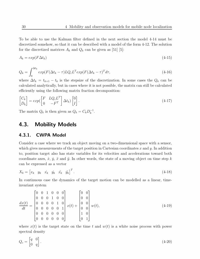
30 4 Mobility and observation models for mobile node localization
To be able to use the Kalman filter defined in the next section the model 4-14 must be
discretized somehow, so that it can be described with a model of the form 4-12. The solution
for the discretized matrices Ak and Qk can be given as [51] [5]:
Ak = exp(F∆tk) (4-15)
Qk =
∫ ∆tk
0
exp(F (∆tk − τ)LQcLT exp(F (∆tk − τ)Tdτ, (4-16)
where ∆tk = tk+1 − tk is the stepsize of the discretization. In some cases the Qk can be
calculated analytically, but in cases where it is not possible, the matrix can still be calculated
efficiently using the following matrix fraction decomposition:[
Ck
Dk
]
= exp(
[
F LQcLT
0 −F T
]
∆tk)
[
0
I
]
. (4-17)
The matrix Qk is then given as Qk = CkD−1k .
4.3. Mobility Models
4.3.1. CWPA Model
Consider a case where we track an object moving on a two-dimensional space with a sensor,
which gives measurements of the target position in Cartesian coordinates x and y. In addition
to, position target also has state variables for its velocities and accelerations toward both
coordinate axes, x, y, x and y. In other words, the state of a moving object on time step k
can be expressed as a vector
Xk =[
xk yk xk yk xk yk]T
. (4-18)
In continuous case the dynamics of the target motion can be modelled as a linear, time-
invariant system
dx(t)
dt=
0 0 1 0 0 0
0 0 0 1 0 0
0 0 0 0 1 0
0 0 0 0 0 1
0 0 0 0 0 0
0 0 0 0 0 0
x(t) +
0 0
0 0
0 0
0 0
1 0
0 1
w(t), (4-19)
where x(t) is the target state on the time t and w(t) is a white noise process with power
spectral density
Qc =
[
q 0
0 q
]
. (4-20)
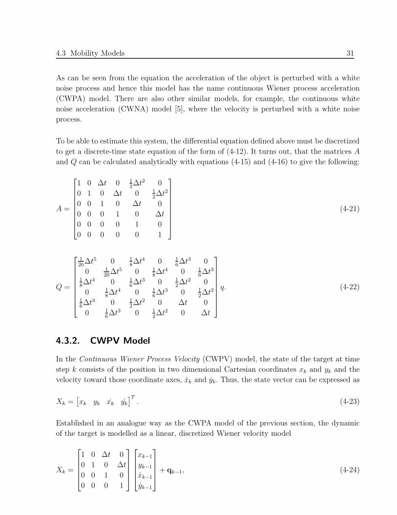
4.3 Mobility Models 31
As can be seen from the equation the acceleration of the object is perturbed with a white
noise process and hence this model has the name continuous Wiener process acceleration
(CWPA) model. There are also other similar models, for example, the continuous white
noise acceleration (CWNA) model [5], where the velocity is perturbed with a white noise
process.
To be able to estimate this system, the differential equation defined above must be discretized
to get a discrete-time state equation of the form of (4-12). It turns out, that the matrices A
and Q can be calculated analytically with equations (4-15) and (4-16) to give the following:
A =
1 0 ∆t 0 12∆t2 0
0 1 0 ∆t 0 12∆t2
0 0 1 0 ∆t 0
0 0 0 1 0 ∆t
0 0 0 0 1 0
0 0 0 0 0 1
(4-21)
Q =
120∆t5 0 1
8∆t4 0 1
6∆t3 0
0 120∆t5 0 1
8∆t4 0 1
6∆t3
18∆t4 0 1
6∆t3 0 1
2∆t2 0
0 18∆t4 0 1
6∆t3 0 1
2∆t2
16∆t3 0 1
2∆t2 0 ∆t 0
0 16∆t3 0 1
2∆t2 0 ∆t
q. (4-22)
4.3.2. CWPV Model
In the Continuous Wiener Process Velocity (CWPV) model, the state of the target at time
step k consists of the position in two dimensional Cartesian coordinates xk and yk and the
velocity toward those coordinate axes, xk and yk. Thus, the state vector can be expressed as
Xk =[
xk yk xk yk]T
. (4-23)
Established in an analogue way as the CWPA model of the previous section, the dynamic
of the target is modelled as a linear, discretized Wiener velocity model
Xk =
1 0 ∆t 0
0 1 0 ∆t
0 0 1 0
0 0 0 1
xk−1
yk−1
xk−1
yk−1
+ qk−1, (4-24)

32 4 Mobility and observation models for mobile node localization
where qk−1 is Gaussian process noise with zero mean and covariance
Q =
13∆t3 0 1
2∆t2 0
0 13∆t3 0 1
2∆t2
12∆t2 0 ∆t 0
0 12∆t2 0 ∆t
q (4-25)
where q is the spectral density of the noise.
4.3.3. Position Model
In the Position (P) model, the state of the target at time step k consists only of the position
in two dimensional Cartesian coordinates xk and yk. Thus, the state vector can be expressed
as
Xk =[
xk yk]T
. (4-26)
Established in an analogue way as Random Walk model, the dynamic of the target is mod-
elled as a linear, discretized Wiener model
Xk =
[
1 0
0 1
] [
xk−1
yk−1
]
+ qk−1, (4-27)
where qk−1 is Gaussian process noise with zero mean and covariance
Q =
[
∆t 0
0 ∆t
]
q (4-28)
where q is the spectral density of the noise.
4.3.4. Coordinated Turn Model
A common way of modelling a turning object is to use the coordinated turn model [5].
The idea is to augment the state vector with a turning rate parameter ω, which has to
be estimated along with the other system parameters (the position and the velocity of the
target). Thus, the joint system vector can be expressed as
Xk =[
xk yk xk yk ωk
]T. (4-29)
The dynamic model for the coordinated turns is
Xk+1 =
1 0 sin(ωk∆t)ωk
cos(ωk∆t)−1ωk
) 0
0 1 1−cos(ωk∆t)ωk
) sin(ωk∆t)ωk
0
0 0 cos(ωk∆t) −sin(ωk∆t) 0
0 0 sin(ωk∆t) cos(ωk∆t) 0
0 0 0 0 1
Xk +
0
0
0
0
1
vk, (4-30)
where vk ∼ N(0, σ2ω) is univariate white Gaussian process noise for the turn rate parameter.
This model is, despite the matrix form, non-linear.

4.4 Measurement Model 33
4.4. Measurement Model
In a wireless ad hoc network, the distance between the mobile and a reference (reachable)
node can be inferred from the received signal strength indicator (RSSI) or pilot signal of the
node. The RSSI, measured in dB, received at the mobile node Ni from the node Nj with
coordinates (xj,k, yj,k) at time k is given by [37]
zij,k = κj − 10γlog10(dij,k) + vi,k, (4-31)
where κj is a constant determined by the transmitted power, wavelength, and gain of the
node Nj, γ is the slope index (tipically γ = 2 for highways and γ = 4 for microcells in a city),
vi,k is the logarithm of the shadowing component which is found to be a zero mean, stationary
Gaussian process with standard deviation σv (from 4-8 dB), and dij,k is the distance between
the mobile nodes Ni and Nj
dij,k =√
(xj,k − xi,k)2 + (yj,k − yi,k)2. (4-32)
All nodes in the group send their pilot signal strength measurements (reference strength
indicator signals) to the reference nodes. In the case with n mobile nodes, and r fixed nodes
having known positions and without communications between the fixed nodes, the overall
observation vector has the form
zk = {zij,k}Lij=1, (4-33)
where L = n ∗ r is the number of measurements. In the developed solutions we do not
consider communications between mobile nodes, hence we exclude the measured distances
between them. The vector form of the observation equation (4-31) is
zk = Hkxk + vk, (4-34)
where the noise vk consists of the path loss and the shadowing component.
Summary
This chapter presented the mathematical fundamentals for the study of localization problem
in Ad Hoc wireless sensor networks. Starting from a discrete-time state space representation,
the Wiener Process and the Coordinated Turn models are discussed. Also, the measurement
model based on the signal strength indicator was established.

5 The application of Kalman-based
schemes to localization
5.1. Theoretical tools
5.1.1. Lateration
This algorithm is based on a very simple idea. For all the mobile nodes, each anchor node
measures the power received from the mobile and draws a circle around itself by computing
the distance (inversion of the path loss model formula). The anchor node assumes that the
mobile should be at one of the points on the circumference of the circle. If the measurement
of the distances is exact (i.e. there is no fading and no shadowing) it is possible to discover
where is the mobile node by the intersection of three circles, given three anchor nodes.
To make the implementation easier, pairs of anchor nodes were considered rather than
triplets. In such a manner, for each pair of anchor nodes it should be possible to calcu-
late two points where the circles overlap: one of this is correct, the other one is false. Then,
for each pair of anchor nodes it is possible to collect two estimated positions for all the
mobile nodes considered. Referring to the collected estimates of an individual mobile node,
the objective is to find which ones are correct and which are false.
The main problem associated with the lateration positioning is that in the presence of fading
and shadowing this method may produce no results at all, i.e. the error in the distance
estimation can prevent the circles overlaping.
5.1.2. Kalman Filter
In the 1960s R.E. Kalman published a paper entitled A new Approach to Linear Filtering and
Prediction Problems (see [26]). In this work the author presented a novel filtering method to
process data for solving problems that deal with measurements hampered by random biases,
with the goal of providing a recursive solution for estimation of linear discrete-time dynamic
systems. A Kalman Filter is an optimal recursive data processing algorithm; each of these
words composes the magical formula that makes one aware of what this filter is:
”data processing algorithms”, this simply means that the Kalman Filter is a set of

5.1 Theoretical tools 35
Figure 5-1: The lateration process
mathematical formulas implemented in software, and the filtering process is therefore
digital;
”recursive”, that is, the filter repeats at each iteration (i.e. at each measurement
done) the same operations;
”optimal”, namely, the Kalman filter achieves the best performance if we assume the
observed process is linear and the measurement noise is white and gaussian.
The purpose of the filter is to estimate a quantity by both the measurement and the a priori
knowledge about the observed phenomenon. The principle followed is to collect and wisely
process the available information. The data process is made up of two stages:
Prediction: a function estimates the state of the Kalman Filter, projecting the quan-
tity for future estimates. During this stage the measurement value of the quantity is
also collected; these steps translate to equations as follows
m−k = Ak−1mk−1
P−k = Ak−1Pk−1A
Tk−1 +Qk−1.
(5-1)
Update: the data collected at the previous stage is weighted by an appropriate coeffi-
cient called the Kalman Gain, determining the estimation for the observed value. The
equations for this stage are:
vk = yk −Hkm−k
Sk = HkP−k HT
k +Rk
Kk = P−k HT
k S−1k
mk = m−k +Kkvk
Pk = P−k −KkSkK
Tk ,
(5-2)

36 5 The application of Kalman-based schemes to localization
where
m−k and P−
k are, respectively, the predicted mean and covariance of the state on the
time step k before taking into account the current measurement.
mk and Pk are, respectively, the estimated mean and covariance of the state on time
step k after taking into account the current measurement.
vk is the innovation or the measurement residual on time step k.
Sk is the measurement prediction covariance on the time step k.
Kk is the filter gain, an indicator of how much the predictions should be corrected on
time step k.
The measurement function is responsible for projecting the state of the filter into the future
and contains information about the observed process. This function describes a mathematical
model of the measurable monitored phenomenon. In this way we can interpret the measure-
ment obtained dynamically and coherently. The Kalman Gain is composed of quantities that
are related to uncertainty both of the measurements and of the model used. We are assuming
an environment impaired by white gaussian noise; therefore we can take into account both
measurement and projection uncertainties referring to the noise and the covariances of the
model respectively.
In certain cases a Gaussian assumption is too primitive, but a Gaussian process only requires
the first and second order statistics (i.e. mean and covariance) to be statistically described.
The Gaussian assumption often allows complex problems to become more tractable. Further-
more, because the real data are influenced by many variables (e.g., scatter noise, multi-path
channel, measurement noise, used device bias, etc.) we can utilize the Central Limit Theorem,
which is at the core of probability theory. This theorem [36], proves that when a number of
independent random variables are added together, their overall effect can be described well
using a Gaussian probability density.
The assumption of white noise leads to some contradictions. This supposition implies noise
values are not correlated in time, e.g. a channel can change from one state to another one
abruptly. The assumption of whiteness also implies that all frequencies have the some power,
i.e. a noise with infinite power. Despite this, the white-noise model is still useful both for
treatment simplicity and because we can overcome the above problems using some ”tricks”.
For instance, any physical system of interest has a bandpass frequency response; we can just
disregard the frequencies outside this band to get away from the requirement to consider
infinite noise power.

5.1 Theoretical tools 37
Note that in this case the predicted and estimated state covariances on different time steps
do not depend on any measurement, so that they could be calculated off-line before making
any measurements provided that the matrices A, Q, R and H are known on those particular
time steps. It is also possible to predict the state of system as many steps ahead as wanted
just by looping the predict step of Kalman filter, but naturally the accuracy of the estimate
decreases with every step.
5.1.3. Kalman Filter for Tracking Problems
A tracking problem, particularly in a wireless environment, is a complex task indeed. On
one hand the power measurements, which are required to determine the mobile positions,
are hampered by more complex noise than white-gaussian; and on the other the algorithm
and the hardware used can introduce bias that is difficult to control. Furthermore trying to
model animated motion is a difficult challenge since feelings, needs, thoughts, and instincts
can make the movements (and of the mobile carried) completely unpredictable. Despite
this, the trade off between simplicity and reliability leads to investigate the Kalman filter
capabilities to track a mobile terminal along an unknown path. The use of the Kalman Filter
to assist in tracking mobile nodes has been proposed before; see [36], [59], [37].
5.1.4. Kalman Filters for Non-linear State Estimation
In many cases interesting dynamic systems are not linear by nature, so the traditional
Kalman filter cannot be applied in the estimation of the state of such systems. In these
kind of systems, one or both the dynamics and the measurement processes can be non-
linear. In this section we describe two extensions to the traditional Kalman filter, which
can be applied for estimating non-linear dynamical systems by forming Gaussian approx-
imations to the joint distribution of the state x and measurement y. First we present the
Extended Kalman filter (EKF), which is based on Taylor series approximation of the joint
distribution, and then the Unscented Kalman filter (UKF), which is based on the unscented
transformation of the joint distribution.
5.1.5. Extended Kalman Filter (EKF)
The extended Kalman filter (see [5], [51]) extends the scope of Kalman filter to non-linear
optimal filtering problems by forming a Gaussian approximation to the joint distribution of
state x and measurements y using a Taylor series based transformation. A first order EKF is
presented using linear approximation; higher order filters are also possible, but not presented
here. The filtering model used in the EKF is
xk = f(xk−1, k − 1) + qk−1
yk = h(xk, k) + rk,(5-3)
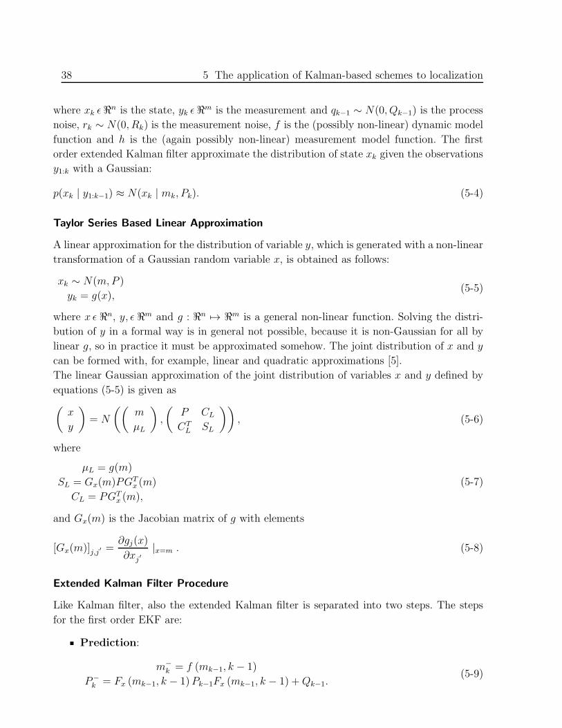
38 5 The application of Kalman-based schemes to localization
where xk ε<n is the state, yk ε<m is the measurement and qk−1 ∼ N(0, Qk−1) is the process
noise, rk ∼ N(0, Rk) is the measurement noise, f is the (possibly non-linear) dynamic model
function and h is the (again possibly non-linear) measurement model function. The first
order extended Kalman filter approximate the distribution of state xk given the observations
y1:k with a Gaussian:
p(xk | y1:k−1) ≈ N(xk | mk, Pk). (5-4)
Taylor Series Based Linear Approximation
A linear approximation for the distribution of variable y, which is generated with a non-linear
transformation of a Gaussian random variable x, is obtained as follows:
xk ∼ N(m,P )
yk = g(x),(5-5)
where x ε <n, y, ε <m and g : <n 7→ <m is a general non-linear function. Solving the distri-
bution of y in a formal way is in general not possible, because it is non-Gaussian for all by
linear g, so in practice it must be approximated somehow. The joint distribution of x and y
can be formed with, for example, linear and quadratic approximations [5].
The linear Gaussian approximation of the joint distribution of variables x and y defined by
equations (5-5) is given as
(
x
y
)
= N
((
m
µL
)
,
(
P CL
CTL SL
))
, (5-6)
where
µL = g(m)
SL = Gx(m)PGTx (m)
CL = PGTx (m),
(5-7)
and Gx(m) is the Jacobian matrix of g with elements
[Gx(m)]j,j′ =∂gj(x)
∂xj′
|x=m . (5-8)
Extended Kalman Filter Procedure
Like Kalman filter, also the extended Kalman filter is separated into two steps. The steps
for the first order EKF are:
Prediction:
m−k = f (mk−1, k − 1)
P−k = Fx (mk−1, k − 1)Pk−1Fx (mk−1, k − 1) +Qk−1.
(5-9)

5.1 Theoretical tools 39
Update:
vk = yk − h(m−k , k)
Sk = Hx(m−k , k)P
−k HT
x (m−k , k) +Rk
Kk = P−k HT
x (m−k , k)S
−1k
mk = m−k +Kkvk
Pk = P−k −KkSkK
Tk ,
(5-10)
where the matrices Fx(m, k − 1) and Hx(m, k) are the Jacobians of f and h, with elements
[Fx(m, k − 1)]j,j′ =∂fj(x, k − 1)
∂xj′
|x=m (5-11)
[Hx(m, k)]j,j′ =∂hj(x, k)
∂xj′
|x=m . (5-12)
Note that the difference between first order EKF and KF is that the matrices Ak and Hk in
KF are replaced with Jacobian matrices Fx(mk−1, k− 1) and Hx(m−k , k)) in EKF. Predicted
mean m−k and residual of prediction vk are also calculated differently in the EKF.
The Limitations of EKF
As discussed in [25], the EKF has some serious drawbacks, which should be kept in mind
when it is used:
1. The linear transformation produces reliable results only when the error propagation
can be well approximated by a linear function. If this condition is not achieved the
performance of the filter can be extremely poor. At worst, its estimates can diverge
altogether.
2. The Jacobian matrices (and Hessian matrices with second order filters) need to exist
so that the transformation can be applied. However, there are cases where this is not
true. For example, the system might be jump-linear and the parameters can change
abruptly [25].
3. In many cases the calculation of Jacobian and Hessian matrices can be a very difficult
process, and its also prone to human errors (both derivation and programming). These
errors are usually very hard to debug, because it its hard to see which parts of the
system produces the errors by looking at the estimates, especially as usually we do not
know which kind of performance we should expect.

40 5 The application of Kalman-based schemes to localization
5.1.6. Unscented Kalman Filter
The unscented Kalman filter (UKF) [25] makes use of the unscented transform described in
section 5.1.6 to give a Gaussian approximation to the filtering solutions of non-linear optimal
filtering problems of the form (same as eq. (5-3), but restated here for convenience)
xk = f(xk−1, k − 1) + qk−1
yk = h(xk, k) + rk,(5-13)
where xk ε<n is the state, yk ε<m is the measurement and qk−1 ∼ N(0, Qk−1) is the Gaussian
process noise, and rk ∼ N(0, Rk) is the Gaussian measurement noise.
Unscented Transform
Like Taylor series based approximation presented above the unscented transform (UT) [25]
can be used for forming a Gaussian approximation to the joint distribution of random vari-
ables x and y, which are defined with equations (5-5). In UT we deterministically choose a
fixed number of sigma points, which capture the desired moments (at least mean and co-
variance) of the original distribution of x exactly. After that we propagate the sigma points
through the non-linear function g and estimate the moments of the transformed variable
from them.
The advantage of UT over the Taylor series based approximation is that UT is better at
capturing the higher order moments caused by the non-linear transform, as discussed in [25].
Also the Jacobian and Hessian matrices are not needed, so the estimation procedure is in
general easier and less error-prone.
The unscented transform can be used to provide a Gaussian approximation for the joint
distribution of variables x and y of the form
(
x
y
)
= N
((
m
µU
)
,
(
P CU
CT
USU
))
. (5-14)
In Eq. 5-14, m = E [x], with E[.] denoting the expected value. Also, m ∈ Rn and P ∈ Rn×n.
The transformation is done as follows:
1. Compute the set of 2n+ 1 sigma points from the columns of the matrix√
(n + λ)P:
χ(0) = m
χ(i) = m+[
√
(n+ λ)P]
i, i = 1, . . . , n
χ(i+n) = m−[
√
(n + λ)P]
i, i = n+ 1, . . . , 2n
(5-15)

5.1 Theoretical tools 41
and the associated weights:
W(0)m = λ�(n+ λ)
W(0)c = λ�(n+ λ) + (1− α2 + β)
W(i)m = 1� {2(n+ λ)} , i = 1, . . . , 2n
W(i)c = 1� {2(n+ λ)} , i = 1, . . . , 2n.
(5-16)
Parameter λ is a scaling parameter, which is defined as
λ = α2(n + κ)− n. (5-17)
The positive constants α, β and κ are used as parameters of the method.
2. Propagate each of the sigma points through the non-linearity as
y(i) = g(x(i)), i = 0, . . . , 2n. (5-18)
3. Calculate the mean and covariance estimates for y as
µU ≈2n∑
i=0
W (i)m y(i) (5-19)
SU ≈2n∑
i=0
W (i)c (y(i) − µU)(y
(i) − µU)T . (5-20)
4. Estimate the cross-covariance between x and y as
SU ≈2n∑
i=0
W (i)c (x(i) −m)(y(i) − µU)
T . (5-21)
The square root of positive definite matrix P is defined as A =√P, where
P = AAT . (5-22)
To calculate the matrix A we can use, for example, lower triangular matrix of the Cholesky
factorization.
The Matrix Form of UT
Let Υ =[
m · · · m]
, Υ ∈ Rn×2n+1 .The unscented transform described above can be
written conveniently in matrix form as follows (see [51] for a proof):
X =[
Υ]
+√c[
0n×1
√P −
√P]
Y = g(X)
µU = Ywm
SU = YWYT
CU = XWYT ,
(5-23)

42 5 The application of Kalman-based schemes to localization
where X is the matrix of sigma points, function g(X) is applied to each column of the
argument matrix separately, c = α2(n + κ), and vector wm and matrix W are defined as
follows:
wm =[
W(0)m · · · W
(2n)m
]T
. (5-24)
W = I−[
wm · · · wm
]
×diag(W(0)c · · · W (2n)
c )
×(I −[
wm · · · wm
]
)T(5-25)
UKF Procedure
Using the matrix form of UT described above the prediction and update steps of the UKF
can computed as follows:
Prediction: Compute the predicted state mean m−k and the predicted covariance P−
k as
X−k =
[
mk−1 · · · mk−1
]
+√c[
0√Pk−1 −√
Pk−1
]
Xk = f(Xk−1, k − 1)
m−k = Xkwm
P−k = XkW
[
Xk
]T
+Qk−1.
(5-26)
Update: Compute the predicted mean µk and covariance of the measurement Sk, and
the cross-covariance of the state and measurement Ck:
X−k =
[
m−k · · · m−
k
]
+√c[
0√
P−k −
√
P−k
]
Y−k = h(X−
k , k)
µk = Y−k wm
Sk = Y−k W
[
Y−k
]T+Rk
Ck = X−k W
[
Y−k
]T.
(5-27)
Then compute the filter gain Kk and the updated state mean mk and covariance Pk:
Kk = CkS−1k
mk = m−k +Kk [yk − µk]
Pk = P−k KkSkK
Tk .
(5-28)

5.1 Theoretical tools 43
5.1.7. Multiple Model Systems
In many practical scenarios it is reasonable to assume that the the model of the system can
change through time somehow. For example, a fighter airplane, which in normal situation
flies with stable flight dynamics, might commence rapid maneuvers when approached by a
hostile missile, or a radar can have a different SNR in some regions of space than in others,
and so on. Such varying system characteristics are hard to describe with only one certain
model, so in estimation one should somehow take into account the possibility that the model
of the system might change.
We now consider systems whose current model is one from a discrete set of n models, which
are denoted by M = {M1, . . . ,Mn}. We assume that for each model M j we have some
prior probability µj0 =
{
M0j
}
. Also the probabilities of switching from model i to model
j in next time step are assumed to be known and denoted by pij = P{
M jk | M i
k−1
}
. This
can be seen as a transition probability matrix of a first order Markov chain characterizing
the mode transitions, and hence systems of this type are commonly referred as Markovian
switching systems. The optimal approach to filtering the states of multiple model system of
this type requires running optimal filters for every possible model sequences, that is, for n
models nk optimal filters must be ran to process the k -th measurement. Hence, some kind
of approximations are needed in practical applications of multiple model systems.
In this section we describe the Interacting Multiple Model (IMM) filter [5] [14], which is
a popular method for estimating systems, whose model changes according to a finite-state,
discrete-time Markov chain. IMM filter can also be used in situations where the unknown
system model structure or its parameters are estimated from a set of candidate models, and
hence it can be also used as a method for model comparison. Initially we start with linear
models, and after that we review the EKF and UKF based non-linear extensions to the
standard IMM-filter.
Linear Systems
We can now modify the equations of linear systems described in (4-12) to have the form
xk = Ajk−1xk−1 + qjk−1
yk = Hjkxk + rjk
(5-29)
where now we have denoted by j the model (or mode) acting during the time step k − 1.
Conditioned on the currently active model we can use the classical Kalman filter (section
5.1.2) for estimating the state of the system on each time step. However, the active model
of the system is not usually known, so we must also estimate it.

44 5 The application of Kalman-based schemes to localization
Interacting Multiple Model (IMM) Filter
IMM-filter [5] is a computationally efficient and in many cases well performing suboptimal
estimation algorithm for Markovian switching systems of the type described above. Basically
it consists of three major steps: interaction (mixing), filtering and combination. In each time
step we obtain the initial conditions for certain model-matched filter by mixing the state
estimates produced by all filters from the previous time step under the assumption that this
particular model is the right model at current time step. Then we perform standard Kalman
filtering for each model, and after that we compute a weighted combination of updated state
estimates produced by all the filters yielding a final estimate for the state and covariance
of the Gaussian density in that particular time step. The weights are chosen according to
the probabilities of the models, which are computed in filtering step of the algorithm. The
equations for each step are as follows:
Interaction: The mixing probabilities µi|jk for each model M i and M j are calculated as
cj =n
∑
i=1
pijµik−1, (5-30)
µi|jk =
1
cjpijµ
ik−1, (5-31)
where µik−1 is the probability of model M i in the time step k−1 and cj a normalization
factor. Now we can compute the mixed inputs (that is, means and covariances) for each
filter as
m0jk−1 =
n∑
i=1
µi|jk mi
k−1, (5-32)
P0jk−1 =
n∑
i=1
µi|jk ×
{
Pik−1 +
[
mik−1 −m0j
k−1
] [
mik−1 −m0j
k−1
]T}
, (5-33)
where mik−1 and Pi
k−1 are the updated mean and covariance for model i at time step
k − 1.
Filtering : Now, for each model M i the filtering is done as[
m−,ik ,P−,i
k
]
= KFp(m0jk−1,P
0jk−1,A
ik−1,Q
ik−1), (5-34)
[
mik,P
ik
]
= KFu(m−,ik−1,P
−,ik−1,yk,H
ik,R
ik), (5-35)
where we have denoted the prediction and update steps (equations ((5-1) and (5-2)) of
the standard Kalman filter with KFp(·) KFu(·), correspondingly. In addition to mean
and covariance we also compute the likelihood of the measurement for each filter as
Λik = N(vi
k; 0,Sik), (5-36)

5.2 Algorithm Description 45
where vik is the measurement residual and and Si
k is the covariance for model M i in
the KF update step. The probabilities of each model M i at time step k are calculated
as
c =
n∑
i=1
Λikci, (5-37)
µik =
1
cΛi
kci, (5-38)
where c is a normalizing factor.
Combination: In the final stage of the algorithm the combined estimate for the state
mean and covariance are computed as
mk =n
∑
i=1
µikm
ik, (5-39)
Pk =n
∑
i=1
µik ×
{
Pik
[
mik −mk
] [
mik −mk
]T}
. (5-40)
Non-linear Systems
The non-linear versions of IMM filter reviewed in previous section can be obtained simply by
replacing the Kalman filter prediction and update steps (in eqs. (5-34) and (5-35)) by their
extended Kalman filter or unscented Kalman filter counterparts, which were reviewed in sec-
tions 5.1.5 and 5.1.6. These algorithms are commonly referred as IMM-EKF and IMM-UKF.
Naturally, this approach introduces some error to the estimations of an already suboptimal
IMM, but it can still provide sufficient accuracy with suitable models.
5.2. Algorithm Description
Using the theoretical concepts presented in the previous section, four localization techniques
were implemented in software for simulation purposes. These schemes employ the observed
RSSI measurements as the way for obtaining the distance of a mobile target with respect to
four reference points. With the distances, the trilateration equations are formed. However,
the RSSI measurements contain uncertainty and noise. So, we integrate the Kalman Filter
to the localization process through four different approaches, using the concepts illustrated
in the previous section.
The analyzed schemes are:
IMM-EKF: EKF based Interacting Multiple Model filter integrated to localization.
The procedure is presented in table 5-1.

46 5 The application of Kalman-based schemes to localization
IMM-UKF: UKF based Interacting Multiple Model filter integrated to localization.
The procedure is presented in table 5-2.
EKF: Extended Kalman filter integrated to localization. The procedure is presented
in table 5-3.
UKF: Unscented Kalman filter integrated to localization. The procedure is presented
in table 5-4.
Table 5-1: IMM-EKF Localization Algorithm Procedure
1. Measure of RSSI values
2. Calculate distance values from RSSI observed values
3. Calculate the mixing probabilities for each model (eq. (5-30) and (5-31))
4. Calculate the mixed initial conditions for the states m0jk−1 and
.. the covariances P 0jk−1 for the models used (5-32) and (5-33))
5. Perform mode-matched filtering with EKF and calculate the corresponding
.. likelihood function (see equations (5-34), (5-35) and (5-36))
6. Update model probabilities (eq. (5-37) and (5-38))
7. Extract combined estimate for the state mean xk = mk and covariance Pk
.. (eq. (5-37) and (5-38))
Table 5-2: IMM-UKF Localization Algorithm Procedure
1. Measure of RSSI values
2. Calculating distance values from RSSI observed values
3. Calculate the mixing probabilities for each model (eq. (5-30) and (5-31))
4. Calculate the mixed initial conditions for the states m0jk−1 and
.. the covariances P 0jk−1 for the models used (5-32) and (5-33))
5. Perform mode-matched filtering with UKF and calculate the corresponding
.. likelihood function (see equations (5-34), (5-35) and (5-36))
6. Update model probabilities (eq. (5-37) and (5-38))
7. Extract combined estimate for the state mean xk = mk and covariance Pk
.. (eq. (5-37) and (5-38))

5.3 Hypothesis Test: ANOVA Analysis 47
Table 5-3: EKF Localization Algorithm Procedure
1. Measure of RSSI values in dB
2. Calculate distance values from RSSI observed values (eq. (4-31))
3. Initialize values for the states x0 and the covariance P0 for the model used
4. Apply EKF procedure using m0 = x0, P0, the distance values and
.. the model parameters (see equations (5-9) and (5-10))
5. Extract the estimated values of the states xk = mk at the k instant
Table 5-4: UKF Localization Algorithm Procedure
1. Measure of RSSI values in dB
2. Calculate distance values from RSSI observed values (eq. (4-31))
3. Initialize values for the states x0 and the covariance P0 for the model used
4. Calculate sigma points and the associated weights (eq. (5-15) and (5-16))
5. Apply UKF procedure using m0 = x0, P0, the distance values and
.. the model parameters (see equations (5-26), (5-27) and (5-28))
6. Extract the estimated values of the states xk = mk at the k instant
5.3. Hypothesis Test: ANOVA Analysis
Analysis of variance (ANalysis Of VAriance - ANOVA) is a general method for studying
sampled-data relationships [10]. The method analyzes the difference between two or more
sample means, achieved by subdividing the total sum of squares. One way ANOVA is the
simplest case. The purpose is to test for significant differences between class means, and this
is done by analysing the variances. Incidentally, if we are only comparing two different means
then the method is the same as the t- test for independent samples [11]. The basis of ANOVA
is the partitioning of sums of squares into between-class (SSb) and within-class (SSw). It
enables all classes to be compared with each other simultaneously rather than individually;
it assumes that the samples are normally distributed. The one-way analysis is calculated in
three steps. First, the sum of squares for all samples, then the within-class cases and, at
last, the between-class cases. For each stage the degrees of freedom df are also determined,
where df is the number of independent ”pieces of information”that go into the estimation
of a parameter. These calculations are performed via the Fisher statistic to analyse the
null hypothesis. The null hypothesis states that there are no differences between means of
different classes, suggesting that the variance of the within-class samples should be identical
to that of the between-class samples (resulting in no between-class discrimination capability).
It must however be noted that small sample sets will produce random fluctuations due to
the assumption of a normal distribution. If dij is the sample for the ith class and jth data

48 5 The application of Kalman-based schemes to localization
point then the total sum of squares is defined as:
SSt =
S∑
i=1
D∑
j=1
(dij −GM)2 (5-41)
with degrees of freedom:
dft = (S D)− 1 (5-42)
where D is the number of data points (assuming equal numbers of data points in each class)
and S is the number of classes and GM is the grand mean:
GM =1
(S D)
S∑
i=1
D∑
j=1
dij. (5-43)
The second stage determines the sum of squares for the within class case, defined as:
SSw =S∑
i=1
D∑
j=1
(dij −Mi)2, (5-44)
where Mi is the ith class mean determined by:
Mi =1
D
D∑
j=1
dij, (5-45)
and the within class df is:
dfw = S(D − 1). (5-46)
The sum of squares for the between class case is:
SSb =
S∑
i=1
D (Mi −GM)2, (5-47)
with the corresponding df of:
dfb = S − 1. (5-48)
Defining the total degrees of freedom dft and the total sum of squares SSt as:
dft = dfb + dfw, (5-49)

5.3 Hypothesis Test: ANOVA Analysis 49
SSt = SSb + SSw. (5-50)
Finally if MSSb is the mean square deviations (or variances) for the between class case, and
MSSw is the reciprocal for the within class case, then:
MSSb =SSb
dfb; MSSw =
SSw
dfw. (5-51)
It is now possible to evaluate the null hypothesis using the Fisher statistic, defined as:
F =MSSb
MSSw
. (5-52)
If F >> 1, then it is likely that differences between class means exist. These results are
then tested for statistical significance or P -value, where the P -value is the probability that a
variate would assume a value greater than or equal to the value observed strictly by chance.
If the P -value is small (eg. P < 0,01 or P < 1%) then this implies that the means differ by
more than would be expected by chance alone. By setting a limit on the P -value, (i.e. 1%)
a critical F value can be determined. The critical value Fcrit is determined (via standard
lookup tables) through the between-class (dfb) and within-class (dfw) df values. Values of
F greater than the critical value denote the rejection of the null hypothesis, which prompts
further investigation into the nature of the differences of the class means. In this way ANOVA
can be used to prune a list of features [55].
Summary
This section presented the application of four different Kalman-based schemes to the local-
ization problem in Ad Hoc wireless sensor networks. All the proposed schemes employ the
multilateration technique as the basis for the unknown position determination. The schemes
are distinguished by the Kalman-scheme implemented, and by the use of a single mobility
model or a set of interacting mobility models. The proposed schemes were:
EKF: Employs Extended Kalman Filter and a single movement model.
UKF: Employs Unscented Kalman Filter and a single movement model.
IMM-EKF: Employs Extended Kalman Filter and the interacting multiple model
technique for the target movement representation.
IMM-EKF: Employs Unscented Kalman Filter and the interacting multiple model
technique for the target movement representation.
THis section enden with the description of the ANOVA analysis, an statistical tool for
studying the relationships between different sets of sampled data.

6 Simulation results
In this chapter, the simulation results of the different localization algorithms are shown and
discussed. Two examples are exhibited with the objective to demonstrate the capability of
the algorithms of tracking a target undergoing different trajectories.
6.1. Wiener Process Models Performance Comparison
In this section, the performance of the P , PV , and PV A models with Extended Kalman
Filter for trajectory tracking will be compared. The benefit of one over the other depends
upon the characteristics of the motion of the object. A system modeled using just P will work
when the position is mostly constant and the velocity can be treated as noise. In the case of a
PV model, it will tend to work better when velocity is mostly constant, and the acceleration
can be treated as noise. PVA on the other hand works better when the acceleration is mostly
constant [?].
6.1.1. Simulation Description
At first, we will explore the performance of the P, PV, and PVA models with an Extended
Kalman Filter. We simulate the two dimensional motion of an object by collecting distance
measurements of the mobile node while physically moving it in a network composed of
8 wireless sensors (see figure 6-1). The range measurement employed is Received Signal
Strength Indicator (RSSI); however, as was discussed in previous sections, the use of RSSI
introduces noise. The distance measurements returned by the sensors fluctuate often and
these measurements are the inputs to the Kalman filters.
RSSI = κj − 10γlog10(dij,k) + vi,k, (6-1)
.
To investigate the positioning capabilities of the implemented RSSI based algorithms the
simulation was set up as reported below. We chose the parameters in order to fit the real
node features and the characteristics of the environment reported in [36]. The distance
measurements were obtained from eq. (6-1) (see section 4.4 for further explanation). All the
algorithms have been tested in 100 scenarios, with randomly created noises, and equal for all
algorithms; the results obtained can therefore be interpreted statistically. We have repeated

6.1 Wiener Process Models Performance Comparison 51
Table 6-1: Simulation parameters for Wiener Process Models Performance Comparison
T Sampling time [s] 0,08s
n Number of samples 50
κj Transmission power [dB] 90
γ Path loss index 2,1060
nsim Number of Monte Carlo runs 100
σv Covariance of the gaussian noise v [dB] 2,0873
the experiments with the same simulation values, but modifying the process noise parameter
q over the Extended Kalman Filter procedure, to gauge its influence on the overall estimation
with the different models.
−2500 −2000 −1500 −1000 −500 0 500−400
−300
−200
−100
0
100
200
300Position
Real trajectoryMeasurementsSensors
Figure 6-1: Simulation testbed for the comparison of the trajectory estimation for P, PV,
and PVA models with an Extended Kalman Filter. The green dots denote a set
of the noisy position observations randomly generated.
The sensors or reference points were placed at fixed coordinates (denoted by +) of the grid as
shown in 6-1. For each of the 50 tested position (see the green dots), distances measurements
were collected from the eight beacons. The measurement noise for each of the sensors was
assumed to be independent of the others. The measurement noise was obtained by taking
the average difference between the actual and estimated distances from the beacons to the
nodes. The process noise matrix Q is more difficult to obtain. Approximate behavior such
as the standard deviation of the position for the P model about the estimated movement
of the object can be used. Of course, the standard deviation of velocity would be applied

52 6 Simulation results
for the PV model, and the standard deviation of the acceleration for the PV A model.
Determination of the correct process noise parameters are key to accurate localization. Here,
we use Q = diag {q}, with q taking values from the vector q =[
50 5 0,5 0,05]T.
6.1.2. Discussion of Results
We have implemented EKF P, PV, and PVA tracking algorithms and performed experiments
extensively. Several metrics were used to compare the performances of the Kalman filters. The
first is the average distance error (DE) in localization per estimate, as defined by equation
(6-2). Another metric that was used is the Root Mean Square Error (RMSE). The benefit of
the RMSE given in equation (6-3) is that the error in localization of the X and Y coordinates
is available. The X and Y RMSE values can be combined through equation (6-4) resulting
in the Net RMSE that describes the net error. An interesting characteristic of the RMSE
is that it is biased towards large errors. A large error make a larger contribution in RMSE
than in average distance error.
DE =Σ√
(xactual − xest)2 + (yactual − yest)2
number of estimates(6-2)
RMSE =
√
Σ(actual − estimated)2
number of estimates(6-3)
Net RMSE =√
x2RMSE + y2RMSE (6-4)
We ran one hundred simulations of the position per value of the noise process q. In table
6-2, the average error metrics for each case are presented. As table 6-2 indicates, the PV
model has the least distance error per estimate and the least NetRMSE and hence the best
localization performance in every case, except when the value of the noise process is q = 0,05.
This is followed closely by the PVA model, and finally the P model. Figure 6-2 shows the
best estimation reached by each model for the different q values evaluated. Figure 6-3 plots
the average Distance Error of the estimation with each model for the different values of q.
Over the performance of the models, we can highlight the following comments:
The value of the process noise parameter q has a deep effect on the estimation capabil-
ities of each model. When the q value is high, meaning that the uncertainty over the
process model is high, all three estimation models have a similar performance. Howev-
er, as the q value decreases, the models with more complete information prevail. The
PV and PVA models, with more rigid kinematic equations, tend to perform better.
This fact is corroborated when the PVA model (more descriptive) reaches the lowest
error values when the noise process parameter has a minimum value of q = 0,05

6.1 Wiener Process Models Performance Comparison 53
The P model estimation decays significantly when the values of the noise parameter
decrease; in fact, the P model only works well when q = 50. This is due to the assump-
tion that velocity and acceleration are just random noise; when the uncertainty in the
trajectory model decrease (lower q), the ability of the P model to keep up with the
reference trajectory is completely reduced.
There are two cases when seems that there is no difference between the estimation with
the different models. For these specific cases, we performed an ANOVA analysis over the
average DE of the estimations. We choose as the null hypothesis the statement that there
are no significant statistical differences between the estimations, and we use a critical value
or Fcrit = 0,05. Remember, if the P -value of the ANOVA is lower than Fcrit, we reject the
null hypothesis. Conversely, if P -value > Fcrit, then the null hypothesis is accepted. See the
results in the paragraphs below.
Table 6-2: Average of the error metrics for the trajectory estimation with P , PV and PV A
models for different values of q
Model DE xRMSE yRMSE NetRMSE q
P 33.6596 28.4742 25.5553 38.3858
PV 32.4624 26.9093 25.3647 37.1278 50
PVA 34.2068 27.3339 27.8196 39.1788
P 38.3033 33.9419 32.6505 47.2804
PV 27.2986 23.4787 20.0342 30.9742 5
PVA 29.9712 25.1152 22.7514 34
P 96.3363 106.2014 79.9403 132.9739
PV 26.3663 20.3114 21.6824 29.9136 0.5
PVA 27.0517 22.2004 20.942 30.6959
P 226.2218 306.2388 93.8838 320.331
PV 46.6378 34.3279 45.2519 56.9912 0.05
PVA 25.0649 20.2785 19.5381 28.4024

54 6 Simulation results
Case 1 - Estimation when q = 50: Figure 6-4 depicts the boxplots and the P -
value of the ANOVA for the different set of estimations with q = 50. Even if the
estimation with the P, PV, and PVA models look very similar from figures 6-2 and
6-3, the P -value indicates that there is a significant statistical difference among the
average Distance Error of the estimations. However, the comparison of P and PVA
data showed no difference between them, with a P -value = 0,25994 > Fcrit = 0,05.
These results favor the PV estimation as the best possible result obtained whit q = 50.
Case 2 - Estimation with PV and PVA models when q = 0,5: Figure 6-5 depicts
the boxplots and the P -value of the ANOVA for only PV and PVA set of estimations
with q = 0,5. As we can see from figures 6-2 and 6-3, the P model performance is lower
than the other two, so we let this data out of the analysys. In this case, the ANOVA
analysis threw a P -value = 0,10608 > Fcrit = 0,05. Therefore, we accept the null
hypothesis, and we conclude that there is no significant statistical difference between
the average of Distance Error estimation for PV and PVA models with q = 0,5
−2500 −2000 −1500 −1000 −500 0 500−400
−200
0
200
400
X
Y
Best Position Estimation with q = 50
−2500 −2000 −1500 −1000 −500 0 500−400
−200
0
200
400
X
Y
Best Position Estimation with q = 5
−2500 −2000 −1500 −1000 −500 0 500−400
−200
0
200
400
X
Y
Best Position Estimation with q = 0.5
−2500 −2000 −1500 −1000 −500 0 500−400
−200
0
200
400
X
Y
Best Position Estimation with q = 0.05
Trajectory
Measurements
faros
Starting point
EKF PVA
EKF PV
EKF P
Figure 6-2: Best trajectory estimation with each model for different values of the q
parameter

6.1 Wiener Process Models Performance Comparison 55
0 20 40 60 80 10020
25
30
35
40
45
Simulation
Ave
rage
DE
Average Distance Error with q = 50
0 20 40 60 80 10020
30
40
50
60
Simulation
Ave
rage
DE
Average Distance Error with q = 5
0 20 40 60 80 1000
50
100
150
Simulation
Ave
rage
DE
Average Distance Error with q = 0.5
P
PV
PVA
0 20 40 60 80 1000
50
100
150
200
250
Simulation
Ave
rage
DE
Average Distance Error with q = 0.05
Figure 6-3: Average Distance Error with the different values of q
25
30
35
40
P PV
p = 0.0089968
25
30
35
40
P PVA
p = 0.25994
25
30
35
40
PV PVA
p = 0.00049858
25
30
35
40
P PV PVA
p = 0.0010814
Figure 6-4: Boxplot and p-value of ANOVA analysis for the Distance Error data of the
different estimations with q = 50

56 6 Simulation results
20
22
24
26
28
30
32
34
36
PV PVA
p = 0.10608 with q = 0.5
Figure 6-5: Boxplot and p-value of ANOVA analysis for the Distance Error data of PV
and PV A estimations with q = 0,5
As a summary, we can conclude that the performance of the three Wiener Process models
evaluated was very similar when the noise process was high; i.e., there is a high uncertainty
over the motion target model. However, as the noise process decreased, the performance of
the different estimation got better for the models including more kinematic parameters (P
and PVA), as this kind of models have a more detailed descriptive level.
6.2. Target Tracking
Next we review a classical filtering application (see, e.g., [?]), in which we track a moving
object with sensors, which measure only the bearings (distances) of the object with respect
positions of the sensors. There is a one moving target in the scene and four sensors for
tracking it. Solving this problem is important, because often more general multiple target
tracking problems can be partitioned into sub-problems, in which single targets are tracked
separately at a time [51].
6.2.1. Simulation Description
Similarly to the scenario presented in section 6.1, we consider one mobile target with four
reference nodes. Respective pilot signal strengths are used between the mobile nodes and

6.2 Target Tracking 57
reference nodes. Two sample mobile trajectories were generated using the Coordinated Turn
Model for the mobile target.
The four Kalman-based algorithms described in the previous chapter are used for locating
the mobile target. The target and the reference nodes transmit RSSI signals, and every node
can receive the signals of the others (a fully communicated one-hop network). The distance
measurements were obtained from the RSSI data and the position of the object was extracted
directly with the additive noise, in the same way as explained in section 6.1. Over 100 Monte
Carlo simulations were performed for each algorithm and trajectory, with the RSSI values
randomly generated in each experiment.
In the estimation we use the following models:
1. Standard Wiener process velocity model with process noise variance q1 = 0,05, whose
purpose is to model the relatively slow turns.
2. A combination of Wiener process velocity model and a coordinated turn model de-
scribed above. The variance of the process noise for the velocity model is set to q2 = 0,01
and for the turning rate parameter in the turning model to qω = 0,15. The estimation
is now done with both the EKF and UKF based IMM filters as the turning model is
non-linear. In both cases the model transition probability matrix is set to
Φ =
[
0,9 0,1
0,1 0,9
]
, (6-5)
and the prior model probabilities are
µ0 =[
0,9 0,1]
. (6-6)
The simulation parameters are described in table 6-3. The position of the object is estimated
with the following methods:
EKF: Extended Kalman filter using the Wiener process velocity model.
UKF: Unscented Kalman filter using the same model as the EKF.
IMM-EKF: EKF based IMM filter using a combination of Wiener process velocity
model and a coordinated turn model.
IMM-UKF: UKF based IMM filter using the same models as IMM-EKF.
The combined position root-mean-square error (RMSE) shown in the equation 6-7 is used to
assess the closeness of the estimated trajectory x, y to to the actual trajectory x, y averaged
over the number of data points n.
RMSE =
√
√
√
√
1
n
n∑
i=1
[(xi − xi)2 + (yi − yi)2]. (6-7)

58 6 Simulation results
Table 6-3: Simulation parameters for Target Tracking
T Sampling time [s] 0,1s
n Number of samples 200
κj Transmission power [dB] 90
γ Path loss index 2,1060
nsim Number of Monte Carlo runs 100
σv Covariance of the gaussian noise v [dB] 2,0873
6.2.2. Results for trajectory 1
Trajectory 1 is generated from a combination between PV Wiener Process Model and a
Coordianted Turn Model as described in table 6-4. The trajectory is depicted in figure 6-6.
We ran 100 Monte Carlo simulations for this trajectory. A sample result of one estimations
is plotted in Figure 6-7. The estimates seem to be very similar for the four Kalman-based
algorithms.
In table 6-5 we have listed the average mean square errors of position estimates over 100
Monte Carlo runs. The histogram of average RMSE of position estimation for each simulation
is plotted in figure 6-8. Also, The average RMSE of velocity estimation for each simulation
is shown in figure 6-9. It can be observed that the estimates of EKF and UKF are identical
in practice. The difference between IMM-UKF and IMM-EKF is trending in the favor of
IMM-UKF. To corroborate this observations, we perform an ANOVA analysis like is going
to be shown in the next subsection.
Table 6-4: Description of Trajectory 1
1. Object starts from origin with velocity (x, y) = (1, 0).
2. At 4s object starts to turn left with rate ω = 1.
3. At 9s object stops turning and moves straight for 2 seconds with a constant
total velocity of one.
4. At 11s objects starts to turn right with rate ω = −1.
5 At 16s object stops turning and moves straight for 4 seconds with the same velocity.

6.2 Target Tracking 59
Table 6-5: Average of RMSE values for Trajectory 1
Algorithm Position RMSE
EFK 0,0587
UKF 0,0586
IMM-EKF 0,0483
IMM-UKF 0,0401
−1 0 1 2 3 4 5 6 7−4
−3
−2
−1
0
1
2
3
4
X
Y
Trajectory 1
Real trajectoryPositions of sensorsStarting position
Figure 6-6: Representation in 2D of Target trajectory 1.

60 6 Simulation results
−1 0 1 2 3 4 5 6 7−4
−3
−2
−1
0
1
2
3
4
X
YPosition estimation results for trayectory 1
TrajectoryEKFUKFIMM−EKFIMM−UKFReference positions
Figure 6-7: A sample of position estimation results for trajectory 1
0 10 20 30 40 50 60 70 80 90 1000.05
0.1
0.15
0.2
0.25
0.3
Number of Simulation
MS
E V
alue
MSE of velocity estimation for trajectory 1
EKFUKFIMM−EKFIMM−UKF
Figure 6-9: MSE of velocity estimation for trajectory 1

6.2 Target Tracking 61
0.03 0.04 0.05 0.06 0.07 0.080
10
20
MSE Values Distribution for trajectory 1 position estimation
MSE EKF
0.03 0.04 0.05 0.06 0.07 0.080
10
20
MSE UKF
0.03 0.04 0.05 0.06 0.07 0.080
10
20
MSE IMM−EKF
0.03 0.04 0.05 0.06 0.07 0.080
10
20
MSE IMM−UKF
Figure 6-8: MSE of position estimation for trajectory 1
ANOVA analysis for trajectory 1
From figures 6-7 and 6-8, we observe that the position estimation trough EKF and UKF is
almost identical. Also, the average error for the IMM-EKF and IMM-UKF seems to be very
close. For these specific cases, we performed an ANOVA analysis over the average DE of the
estimations. As we did in the section 6.1, we choose as the null hypothesis the affirmation
that there are no significant statistical differences between the estimations, and we use a
critical value or Fcrit = 0,05. Remember, if the the P -value of the ANOVA is lower than
Fcrit, we reject the null hypothesis. Conversely, if P -value > Fcrit, the the null hypothesis is
accepted. See the results in the paragraphs below.
Figure 6-10 depicts the boxplots and the P -value of the ANOVA for the different set of
estimations with the four different filters for trajectory 1. Even if the estimations between
subsets look very similar, the P -value for the different combinations of datasets indicates
that there is a significant statistical difference among the average error of the estimations.
However, the comparison of EKF and UKF data showed no difference between them, with a
P -value = 0,96013 > Fcrit = 0,05. These results favor the IMM-UKF estimation as the best
possible result obtained for trajectory 1.

62 6 Simulation results
0.04
0.05
0.06
0.07
0.08
EKF UKF
p = 0.96013
0.04
0.06
0.08
EKF IMM−EKF
p = 6.9944e−15
0.04
0.06
0.08
EKF IMM−UKF
p = 0
0.04
0.06
0.08
UKF IMM−EKF
p = 9.4369e−15
0.04
0.06
0.08
UKF IMM−UKF
p = 0
0.04
0.06
0.08
IMM−EKF IMM−UKF
p = 6.6407e−12
Figure 6-10: Boxplots of MSE distributions for ANOVA analysis of position estimation for
trajectory 1
6.2.3. Results for trajectory 2
Trajectory 2 is also generated from a combination between PV Wiener Process Model and a
Coordinated Turn Model as described in table 6-6. The trajectory is depicted in figure 6-11.
We ran 100 Monte Carlo simulations for this trajectory. A sample result of one estimations is
plotted in Figure 6-12. The estimates are very similar for the four Kalman-based algorithms,
even more than the previous case. In fact, the results of each method are barely discriminated
one from the others.
Table 6-6: Description of Trajectory 2
1. Object starts from origin with velocity (x, y) = (1, 1).
2. At 4s object starts to turn left with rate ω = 0,1555 and velocity (x, y) = (−1,−1).
3. At 9s object stops turning and moves straight for 2 seconds with a constant
total velocity of one.
4. At 11s objects starts to turn right with rate ω = −0,1555.
5 At 16s object stops turning and moves straight for 4 seconds with the same velocity.

6.2 Target Tracking 63
Table 6-7: Average of RMSE values for Trajectory 2
Algorithm Position RMSE
EFK 0,0339
UKF 0,0339
IMM-EKF 0,0259
IMM-UKF 0,0249
In table 6-7 we have listed the average mean square errors of position estimates over 100
Monte Carlo runs. The histogram of average RMSE of position estimation for each simulation
is plotted in figure 6-8. Also, the average RMSE of velocity estimation for each simulation
is shown in figure 6-9.
For the states representing the velocity over each axis, the IMM based methods hold a
clearly advantage over EKF and UKF. This could be expected, as the IMM techniques rely
on the interaction of more mobility models, and thus can extract more information. As in
the previous section, it can be observed that the estimates of EKF and UKF are identical
in practice. However, there is no appreciable difference between IMM-UKF and IMM-EKF,
although the performance of the latter two methods is better than the former two. Again, to
corroborate this observations, we perform the ANOVA analysis that is being shown shown
in the next subsection.
−2 0 2 4 6 8 10 12 14 16−5
0
5
10
15
20
25
X
Y
Trajectory 2
Real trajectoryPositions of sensorsStarting position
Figure 6-11: Representation in 2D of Target trajectory 2.

64 6 Simulation results
0 5 10 15−5
0
5
10
15
20
25
X
YPosition estimation results for trajectory 2 with variance = 0.5
TrajectoryEKFUKFIMM−EKFIMM−UKFReference positions
Figure 6-12: A sample of position estimation results for trajectory 2
0.02 0.025 0.03 0.035 0.04 0.045 0.05 0.0550
10
20
MSE Values Distribution for trajectory 2 position estimation
MSE EKF
0.02 0.025 0.03 0.035 0.04 0.045 0.05 0.0550
10
20
MSE UKF
0.02 0.025 0.03 0.035 0.04 0.045 0.05 0.0550
10
20
MSE IMM−EKF
0.02 0.025 0.03 0.035 0.04 0.045 0.05 0.0550
10
20
MSE IMM−UKF
Figure 6-13: MSE of position estimation for trajectory 2

6.2 Target Tracking 65
0 10 20 30 40 50 60 70 80 90 1000.02
0.04
0.06
0.08
0.1
0.12
0.14
0.16
0.18
Number of Simulations
MS
E V
alue
sMSE of velocity estimation for trajectorie 2
EKFUKFIMM−EKFIMM−UKF
Figure 6-14: MSE of velocity estimation for trajectory 2
ANOVA analysis for trajectory 2
From figures 6-12 and 6-13, we observe that the position estimation trough EKF and UKF
is almost identical. Also, the average error for the IMM-EKF and IMM-UKF seems to be
equal. For these specific cases, we performed an ANOVA analysis over the average error
of the estimations. Again, we choose as the null hypothesis the affirmation that there are
no significant statistical differences between the estimations, and we use a critical value or
Fcrit = 0,05.
Figure 6-15 depicts the boxplots and the P -value of the ANOVA for the different set of
estimations with the four different filters for trajectory 2. Like the previous case, a P -value
of 0,9606 shows that there is no significant statistical difference between the estimation
with EKF and UKF for this case. Besides this, the null hypothesis is accepted also for the
comparison of IMM-EKF and IMM-UKF, with a P -value = 0,82111, meaning the estimation
results for these two models is statistically identical. So, there is no clear-cut better method
for estimation of trajectory 2: both IMM-based models perform better than the others.

66 6 Simulation results
0.03
0.04
0.05
EKF UKF
p = 0.9696
0.03
0.04
0.05
EKF IMM−EKF
p = 4.1488e−010
0.03
0.04
0.05
EKF IMM−UKF
p = 1.1106e−010
0.03
0.04
0.05
UKF IMM−EKF
p = 3.325e−010
0.03
0.04
0.05
UKF IMM−UKF
p = 8.8531e−011
0.03
0.04
0.05
IMM−EKFIMM−UKF
p = 0.82111
Figure 6-15: Boxplots of MSE distributions for ANOVA analysis of position estimation for
trajectory 2
Summary
It has been show that the four Kalman-based schemes present similar estimation results for
the two different trajectories studied. A case could be made for either method, but the choice
of the best one depends on the designer’s criteria. The IMM-UKF yields the best results, and
the Multiple Model algorithms performed better than those with one-model. Besides this, it
should be noted that the performance of each tested method could be tuned by optimizing
their parameters (e.g. variance of process noise of dynamic models, values of model transition
matrix in IMM, etc.) more carefully, so the performance differences could change radically.
Still, it is clear that the Kalman filter does actually work also with (at least some) non-
linear dynamic and measurement models, and should be considered as a standard location
estimation method for multiple model systems. Also, one should prefer IMM-UKF over IMM-
EKF as the performance is (at least in these examples) better, although his computation
could be higher in some cases.

7 Conclusions and future work
The aim of this thesis was to present an overview of a collection of tools used in the problem of
target tracking. Under this thesis scope, several algorithms for target tracking were studied.
This chapter will thus emphasize the main results drawn from the algorithms studied, bearing
in mind that the validity of these conclusions may be limited to the scenarios simulated.
7.1. Conclusions
The Kalman filter is capable of localizing using noisy distance measurements in sensor
networks. The PV Wiener Process model with Extended Kalman filter was found
to have the best performance over the other Wiener Process model in the studied
examples. However, depending on the motion of the tracked object the PV or PVA
model could be better.
The process noise parameters allow the Kalman filter to project the position of the
object in the next time instant. If the proper process noise parameters are not used,
the performance of the Kalman filters will be severely affected.
The Kalman-based localization algorithms all revealed capable trackers under target
motion uncertainty. The first couple of Kalman-based algorithms (EKF and UKF)
are the most limited, since they assume the target motion is governed by a constant
pattern, i.e., the algorithms only use an unique model to estimate the mobile target
trajectory . The other two schemes (IMM-EKF and IMM-UKF) have more complex
concepts, even though they are not computationally more complex (when using a low
number of models). Their tracking capability appears to be better, since they assume
the target can have multiple maneuver motions.
Regarding the performance comparison shown in chapter 6, this results represent only
an example since the algorithms may have different responses for different target mo-
tions. In the simulations performed in this thesis, there is no sensible difference between
EKF and UKF. Given the availability of more resources (because they had multiple
mobility models), the IMM-based algorithms got better results than EKF and UKF.
This suggests that there is a sensible advantage for the use of this Multiple Model tech-
niques in localization schemes for Ad-Hoc sensor networks over the one-model based
techniques.

68 7 Conclusions and future work
Kalman filtering is an interesting and powerful method to optimally and dynamically
process data hampered by white gaussian noise. Filtering also allows one to interpret
measurements coherently with a mathematical model of the observed phenomenon.
However, as a downside, the performance of the Kalman Filter depends on tuning
parameters and on the model used to describe the process of interest. It is possible
using Kalman filtering to realize tracking applications, achieving a good performance
after a specific delay to achieve the best filter state.
7.2. Future Work
The additional research that can be performed in this area is vast. There are several addi-
tional topics to extend this thesis work, they are:
1. Test further and study even in more depth the algorithms in simulation en-
vironment: more simulations could be realized, specially for the IMM Kalman-based
algorithms, but with the intervention of other kind of ranging signals different than
RSSI. Also further algorithm development could be done in order to study its perfor-
mance in the presence of the phenoms affecting the RSSI signals, just like interferences,
fading and multipath effects.
Regarding this performance improvement, it would be interesting to analyze possible
mathematical designs of the model probability thresholds, characteristic of the IMM
algorithms, and study whether they should be static or adaptive, for instances, if there
is a high uncertainty on the state estimate, the thresholds can be relaxed.
2. Analyze the algorithms performance in a real life implementation: Since all
the discussed algorithms, are studied in environments that try to simulate a real life
situation, it would be valuable to analyze their performances in a real life application.
It would be interesting to implement the algorithms using real sensor measurements
and real targets, and test their capability and robustness.
3. Study alternative algorithms: there are a lot to choose from, more or less document-
ed and more or less studied. An interesting subject with plenty of room for exploration
is the study of more alternative techniques such as the Monte Carlo techniques known
as Particle Filtering [20], which have drawn the attention of the tracking community.

Bibliografıa
[1] I. F. Akyildiz, W. Su, Y. Sankarasubramaniam, and E. Cayirci. Wireless sensor net-
works: a survey. Computer Networks, 38:393–422, 2002.
[2] I. F Akyildiz and Xudong Wang. A survey on wireless mesh networks. Communications
Magazine, IEEE, 43(9):S23 – S30, September 2005.
[3] Jeffrey Antol, Philip Calhoun, John Flick, Gregory Hajos, Richard Kolacinski, David
Minton, Rachel Owens, and Jennifer Parker. Low cost mars surface exploration: The
mars tumbleweed. Tech. Report NASA/TM-2003-212411, NASA STI Program, Langley
Research Center, 2003.
[4] Aline Baggio and Koen Langendoen. Monte carlo localization for mobile wireless sensor
networks. Ad Hoc Netw., 6(5):718–733, 2008.
[5] Yaakov Bar-Shalom and Xiao-Rong Li. Estimation with Applications to Tracking and
Navigation. John Wiley & Sons, Inc., New York, NY, USA, 2001.
[6] Y. Baudoin. Information architecture for sensor and mobile robotic systems facing
the humanitarian demining problem. In Information and Communications Technolo-
gy, 2005. Enabling Technologies for the New Knowledge Society: ITI 3rd International
Conference on, pages 473 –493, December 2005.
[7] O. Bondarenko, S. Kininmonth, and M. Kingsford. Underwater sensor networks,
oceanography and plankton assemblages. In Intelligent Sensors, Sensor Networks and
Information, 2007. ISSNIP 2007. 3rd International Conference on, pages 657 –662,
December 2007.
[8] G. Brasche. Trends and challenges of wireless sensor networks. In Applications and
Services in Wireless Networks, 2008. ASWN ’08. Eighth International Workshop on,
pages 7 –7, October 2008.
[9] M. C Bulan and H. Temeltas. Localization mobile vehicles in a wireless sensor networks
based on hop-count and artificial potentials method. In Control and Automation, 2009.
ICCA 2009. IEEE International Conference on, pages 1417 –1422, December 2009.
[10] G. M. Clarke and D. Cooke. A Basic Course in Statistics. A Hodder Arnold Publication,
1998.

70 Bibliografıa
[11] Paul R. Cohen. Empirical Methods for Artificial Intelligence (Bradford Books). The
MIT Press, 1995.
[12] L. Doherty, K. S.J pister, and L. El Ghaoui. Convex position estimation in wireless
sensor networks. In INFOCOM 2001. Twentieth Annual Joint Conference of the IEEE
Computer and Communications Societies. Proceedings. IEEE, volume 3, pages 1655
–1663 vol.3, 2001.
[13] D. Estrin, L. Girod, G. Pottie, and M. Srivastava. Instrumenting the world with wire-
less sensor networks. In Acoustics, Speech, and Signal Processing, 2001. Proceedings.
(ICASSP ’01). 2001 IEEE International Conference on, volume 4, pages 2033 –2036
vol.4, 2001.
[14] Joana Barbosa Bastos Gomes. An Overview on Target Tracking using Multiple Mod-
el methods. Master thesis in electrical and computer engineering, Instituto Superior
Tecnico, October 2008.
[15] V. C Gungor and G. P Hancke. Industrial wireless sensor networks: Challenges, design
principles, and technical approaches. Industrial Electronics, IEEE Transactions on,
56(10):4258 –4265, October 2009.
[16] P. Gupta and P. R Kumar. The capacity of wireless networks. Information Theory,
IEEE Transactions on, 46(2):388 –404, March 2000.
[17] F. Gustafsson and F. Gunnarsson. Mobile positioning using wireless networks: possi-
bilities and fundamental limitations based on available wireless network measurements.
Signal Processing Magazine, IEEE, 22(4):41 – 53, July 2005.
[18] M. Hanssmann, Sokwoo Rhee, and Sheng Liu. No wiring constraints. Industry Appli-
cations Magazine, IEEE, 15(4):60 –65, August 2009.
[19] Jeng-Cheng Hsieh, Chih-Ming Chen, and Hsiao-Fang Lin. Social interaction mining
based on wireless sensor networks for promoting cooperative learning performance in
classroom learning environment. In Wireless, Mobile and Ubiquitous Technologies in
Education (WMUTE), 2010 6th IEEE International Conference on, pages 219 –221,
April 2010.
[20] Lingxuan Hu and David Evans. Localization for mobile sensor networks. In MobiCom
’04: Proceedings of the 10th annual international conference on Mobile computing and
networking, page 45–57, New York, NY, USA, 2004. ACM.
[21] Chi-Fu Huang and Yu-Chee Tseng. The coverage problem in a wireless sensor network.
In Proceedings of the 2nd ACM international conference on Wireless sensor networks
and applications, WSNA ’03, page 115–121, New York, NY, USA, 2003. ACM.

Bibliografıa 71
[22] Huiping Huang, Shide Xiao, Xiangyin Meng, and Ying Xiong. A remote home security
system based on wireless sensor network and GSM technology. In Networks Security
Wireless Communications and Trusted Computing (NSWCTC), 2010 Second Interna-
tional Conference on, volume 1, pages 535 –538, April 2010.
[23] M. A Hussain, P. khan, and Kwak kyung Sup. WSN research activities for military
application. In Advanced Communication Technology, 2009. ICACT 2009. 11th Inter-
national Conference on, volume 01, pages 271 –274, February 2009.
[24] Philo Juang, Hidekazu Oki, Yong Wang, Margaret Martonosi, Li Shiuan Peh, and Daniel
Rubenstein. Energy-efficient computing for wildlife tracking: design tradeoffs and early
experiences with ZebraNet. In Proceedings of the 10th international conference on Ar-
chitectural support for programming languages and operating systems, ASPLOS-X, page
96–107, New York, NY, USA, 2002. ACM.
[25] S. J Julier and J. K Uhlmann. Unscented filtering and nonlinear estimation. Proceedings
of the IEEE, 92(3):401 – 422, March 2004.
[26] Rudolph Emil Kalman. A new approach to linear filtering and prediction problems.
Transactions of the ASME–Journal of Basic Engineering, 82(Series D):35–45, 1960.
[27] Holger Karl and Andreas Willig. Protocols and Architectures for Wireless Sensor Net-
works. John Wiley & Sons, 2005.
[28] Kwangsoo Kim, Jongarm Jun, Sunjoong Kim, and B. Y Sung. Medical asset tracking
application with wireless sensor networks. In Sensor Technologies and Applications,
2008. SENSORCOMM ’08. Second International Conference on, pages 531 –536, August
2008.
[29] N. Kurata, S. Saruwatari, and H. Morikawa. Ubiquitous structural monitoring using
wireless sensor networks. In Intelligent Signal Processing and Communications, 2006.
ISPACS ’06. International Symposium on, pages 99 –102, December 2006.
[30] J. F Kurose and K. W Ross. Computer networking: a top-down approach. Pearson
Education, 2009.
[31] Koen Langendoen and Niels Reijers. Distributed localization in wireless sensor networks:
a quantitative comparison. Comput. Netw., 43(4):499–518, 2003.
[32] Y. K Leow and Ying Shang. Mobile robot tracking in wireless sensor networks. In
Networking, Sensing and Control (ICNSC), 2010 International Conference on, pages
313 –318, April 2010.
72 Bibliografıa
[33] Alan Mainwaring, David Culler, Joseph Polastre, Robert Szewczyk, and John Ander-
son. Wireless sensor networks for habitat monitoring. In Proceedings of the 1st ACM
international workshop on Wireless sensor networks and applications, WSNA ’02, page
88–97, New York, NY, USA, 2002. ACM.
[34] E. D Manley, H. A Nahas, and J. S Deogun. Localization and tracking in sensor systems.
In Sensor Networks, Ubiquitous, and Trustworthy Computing, 2006. IEEE International
Conference on, volume 2, page 237 –242, June 2006.
[35] Guoqiang Mao, Barıs Fidan, and Brian D. O Anderson. Wireless sensor network local-
ization techniques. Comput. Netw., 51(10):2529–2553, 2007.
[36] Riccardo Masiero. RSSI Based Tracking Algorithms for Wireless Sensor Networks:
Theoretical Aspects and Performance Evaluation. Master thesis in telecommunication
engineering, University of Padova,, Italy, 2007.
[37] L. Mihaylova, D. Angelova, C. N Canagarajah, and D. R Bull. Algorithms for mobile
nodes Self-Localisation in wireless ad hoc networks. In Information Fusion, 2006 9th
International Conference on, pages 1 –7, July 2006.
[38] David Moore, John Leonard, Daniela Rus, and Seth Teller. Robust distributed network
localization with noisy range measurements. In SenSys ’04: Proceedings of the 2nd
international conference on Embedded networked sensor systems, page 50–61, New York,
NY, USA, 2004. ACM.
[39] M. R Morelande, B. Moran, and M. Brazil. Bayesian node localisation in wireless
sensor networks. In Acoustics, Speech and Signal Processing, 2008. ICASSP 2008. IEEE
International Conference on, page 2545 –2548, 2008.
[40] C. Morelli, M. Nicoli, V. Rampa, and U. Spagnolini. Hidden markov models for radio
localization in mixed LOS/NLOS conditions. Signal Processing, IEEE Transactions on,
55(4):1525 –1542, April 2007.
[41] D. Niculescu. Positioning in ad hoc sensor networks. Network, IEEE, 18(4):24 – 29,
August 2004.
[42] D. Niculescu and B. Nath. Ad hoc positioning system (APS). In Global Telecommuni-
cations Conference, 2001. GLOBECOM ’01. IEEE, volume 5, pages 2926 –2931 vol.5,
2001.
[43] Dragos Niculescu and Badri Nath. Error characteristics of ad hoc positioning systems
(aps). In MobiHoc ’04: Proceedings of the 5th ACM international symposium on Mobile
ad hoc networking and computing, page 20–30, New York, NY, USA, 2004. ACM.

Bibliografıa 73
[44] F. Osterlind, E. Pramsten, D. Roberthson, J. Eriksson, N. Finne, and T. Voigt. Inte-
grating building automation systems and wireless sensor networks. In Emerging Tech-
nologies and Factory Automation, 2007. ETFA. IEEE Conference on, pages 1376 –1379,
September 2007.
[45] N. Patwari, J. N Ash, S. Kyperountas, A. O. Hero, R. L Moses, and N. S Correal. Lo-
cating the nodes: cooperative localization in wireless sensor networks. Signal Processing
Magazine, IEEE, 22(4):54 – 69, July 2005.
[46] N. Patwari, A. O. Hero, M. Perkins, N. S Correal, and R. J O’Dea. Relative loca-
tion estimation in wireless sensor networks. Signal Processing, IEEE Transactions on,
51(8):2137 – 2148, August 2003.
[47] Neal Patwari. Location Estimation in Sensor Networks. Electrical engineering PhD
thesis, University of Michigan, USA, 2005.
[48] N. B Priyantha, H. Balakrishnan, E. D Demaine, and S. Teller. Mobile-assisted local-
ization in wireless sensor networks. In INFOCOM 2005. 24th Annual Joint Conference
of the IEEE Computer and Communications Societies. Proceedings IEEE, volume 1,
pages 172 – 183 vol. 1, March 2005.
[49] K. Romer and F. Mattern. The design space of wireless sensor networks. Wireless
Communications, IEEE, 11(6):54 – 61, December 2004.
[50] Kay Romer. The lighthouse location system for smart dust. In Proceedings of the
1st international conference on Mobile systems, applications and services, MobiSys ’03,
page 15–30, New York, NY, USA, 2003. ACM.
[51] Simo Sarkka. Recursive Bayesian Inference on Stochastic Differential Equations. PhD
thesis in technology, Helsinki University of Technology, Espoo, Finland, 2006.
[52] Andreas Savvides, Chih-Chieh Han, and Mani B Strivastava. Dynamic fine-grained
localization in Ad-Hoc networks of sensors. In Proceedings of the 7th annual interna-
tional conference on Mobile computing and networking, MobiCom ’01, page 166–179,
New York, NY, USA, 2001. ACM.
[53] Andreas Savvides, Heemin Park, and Mani B Srivastava. The bits and flops of the n-
hop multilateration primitive for node localization problems. In WSNA ’02: Proceedings
of the 1st ACM international workshop on Wireless sensor networks and applications,
page 112–121, New York, NY, USA, 2002. ACM.
[54] Y. Shang, W. Rumi, Y. Zhang, and M. Fromherz. Localization from connectivity in
sensor networks. Parallel and Distributed Systems, IEEE Transactions on, 15(11):961
– 974, November 2004.

74 Bibliografıa
[55] Jamie Shutler. One way ANOVA - analysis of variance.
http://homepages.inf.ed.ac.uk/rbf/CVonline/LOCAL COPIES/SHUTLER2/node1.html,
2002. In CVonline: On-Line Compendium of Computer Vision [Online].
[56] Dongjin Son, Bhaskar Krishnamachari, and John Heidemann. Experimental study of
concurrent transmission in wireless sensor networks. In In Proc. ACM SenSys, page
237–250. ACM Press, 2006.
[57] K. Wac, R. Bults, B. van Beijnum, I. Widya, V. Jones, D. Konstantas, M. Vollenbroek-
Hutten, and H. Hermens. Mobile patient monitoring: The MobiHealth system. In
Engineering in Medicine and Biology Society, 2009. EMBC 2009. Annual International
Conference of the IEEE, pages 1238 –1241, September 2009.
[58] T. O Walker, M. Tummala, and J. McEachen. Energy efficiency of centralized and dis-
tributed computation in unattended Multi-Hop wireless sensor networks for battlefield
monitoring. In System Sciences (HICSS), 2010 43rd Hawaii International Conference
on, pages 1 –9, January 2010.
[59] Jiangwen Wan, Ning Yu, Renjian Feng, Yinfeng Wu, and Changming Su. Localization
refinement for wireless sensor networks. Computer Communications, 32(13-14):1515 –
1524, 2009.
[60] Nen-Chung Wang and Si-Ming Wang. An efficient location-aided routing protocol for
mobile ad hoc networks. In Parallel and Distributed Systems, 2005. Proceedings. 11th
International Conference on, volume 1, pages 335 – 341 Vol. 1, July 2005.
[61] G. Werner-Allen, K. Lorincz, M. Ruiz, O. Marcillo, J. Johnson, J. Lees, and M. Welsh.
Deploying a wireless sensor network on an active volcano. Internet Computing, IEEE,
10(2):18 – 25, April 2006.
[62] Jiyoung Yi, Sungwon Yang, and Hojung Cha. Multi-hop-based monte carlo localization
for mobile sensor networks. In Sensor, Mesh and Ad Hoc Communications and Net-
works, 2007. SECON ’07. 4th Annual IEEE Communications Society Conference on,
pages 162 –171, June 2007.
[63] Saleh Yousefi, Mahmoud Siadat Mousavi, and Mahmood Fathy. Vehicular ad hoc net-
works (VANETs): challenges and perspectives. In ITS Telecommunications Proceedings,
2006 6th International Conference on, pages 761 –766, June 2006.
[64] Z. R Zaidi and B. L Mark. A mobility tracking model for wireless ad hoc networks. In
Wireless Communications and Networking, 2003. WCNC 2003. 2003 IEEE, volume 3,
pages 1790 –1795 vol.3, March 2003.


![Partial discharge detection and localization using ... › 70376 › 1 › Mohamed_etal_IEEE_IEM… · proposed to be less than 1 meter, [7]. Individual sensor nodes are usually hardware](https://static.fdocuments.net/doc/165x107/60dd962c5d8c9f40b80123e6/partial-discharge-detection-and-localization-using-a-70376-a-1-a-mohamedetalieeeiem.jpg)


