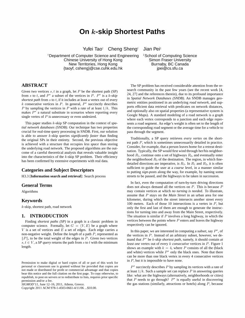
On k-skip Shortest Paths

Yufei Tao† Cheng Sheng† Jian Pei‡†Department of Computer Science and Engineering ‡School of Computing Science

Chinese University of Hong Kong Simon Fraser UniversityNew Territories, Hong Kong Burnaby, BC Canada

taoyf, csheng@cse.cuhk.edu.hk jpei@cs.sfu.ca

ABSTRACTGiven two vertices s, t in a graph, let P be the shortest path (SP)from s to t, and P a subset of the vertices in P . P is a k-skipshortest path from s to t, if it includes at least a vertex out of everyk consecutive vertices in P . In general, P succinctly describesP by sampling the vertices in P with a rate of at least 1/k. Thismakes P a natural substitute in scenarios where reporting everysingle vertex of P is unnecessary or even undesired.

This paper studies k-skip SP computation in the context of spa-tial network databases (SNDB). Our technique has two propertiescrucial for real-time query processing in SNDB. First, our solutionis able to answer k-skip queries significantly faster than findingthe original SPs in their entirety. Second, the previous objectiveis achieved with a structure that occupies less space than storingthe underlying road network. The proposed algorithms are the out-come of a careful theoretical analysis that reveals valuable insightinto the characteristics of the k-skip SP problem. Their efficiencyhas been confirmed by extensive experiments with real data.

Categories and Subject DescriptorsH3.3 [Information search and retrieval]: Search process

General TermsAlgorithms

Keywordsk-skip, shortest path, road network

1. INTRODUCTIONFinding shortest paths (SP) in a graph is a classic problem in

computer science. Formally, let G = (V,E) be a graph whereV is a set of vertices and E a set of edges. Each edge carries anon-negative weight. Define the length of a path P , represented as‖P‖, to be the total weight of the edges in P . Given two verticess, t ∈ V , a SP query returns the path from s to t with the minimumlength.

Permission to make digital or hard copies of all or part of this work forpersonal or classroom use is granted without fee provided that copies arenot made or distributed for profit or commercial advantage and that copiesbear this notice and the full citation on the first page. To copy otherwise, torepublish, to post on servers or to redistribute to lists, requires prior specificpermission and/or a fee.SIGMOD’11, June 12–16, 2011, Athens, Greece.Copyright 2011 ACM 978-1-4503-0661-4/11/06 ...$10.00.

The SP problem has received considerable attention from the re-search community in the past few years (see the recent work [4,24, 27] and the references therein), due to its profound importancein Spatial Network Databases (SNDB). An SNDB manages geo-metric entities positioned in an underlying road network, and sup-ports efficient data retrieval with predicates on network distances,and optionally also on spatial properties (a representative system isGoogle Maps). A standard modeling of a road network is a graphwhere each vertex corresponds to a junction and each edge repre-sents a road segment. An edge’s weight is often set to the length ofthe corresponding road segment or the average time for a vehicle topass through the segment.

Traditionally, a SP query retrieves every vertex on the short-est path P , which is sometimes unnecessarily detailed in practice.Consider, for example, that a person leaves home for a retreat desti-nation. Typically, the SP would first wind through her/his neighbor-hood R1, continue onto a set of highways R2, and eventually enterthe neighborhood R3 of the destination. The region, in which fine-detailed directions are imperative, is R3. In R1 and R2, it is oftensufficient to guide the user at a coarse level, in a manner similarto putting sign-posts along the way, for example, by naming somestreets to be passed, and the highways to be taken in succession.

In fact, even the computation of turn-by-turn driving directionsdoes not always demand all the vertices on P . This is because Pmay contain vertices at which no turning is needed. To illustrate,assume that P stays on the Main Street in an urban area for onekilometer, during which the street intersects another street every100 meters. Each of those 10 intersections is a vertex in P , butonly the first and last of them are enough to generate the instruc-tions for turning into and away from the Main Street, respectively.The situation is similar if P involves a long highway, in which thevertices between the points where P enters and leaves the highwayrespectively can be ignored.

In this paper, we are interested in computing a subset, say P, ofthe vertices in P . Instead of an arbitrary subset, however, we de-mand that P ∗ be k-skip shortest path, namely, it should contain atleast one vertex out of every k consecutive vertices in P . Figure 1shows an example with k = 4, where P consists of all the (blackand white) vertices while P only the black ones. Note that therecan be more than one black vertex in every 4 consecutive verticesin P , but it is impossible to have none.

P succinctly describes P by sampling its vertices with a rate ofat least 1/k. Such a sample set can replace P in answering querieslike: what are the highways (alternatively, neighborhoods or cities)that P needs to go through? P is equally useful in discoveringthe gas stations (similarly, attractions or hotels) along P , because

s

t

Figure 1: The black vertices constitute a 4-skip shortest path

it is often sufficient to find the stations close to the vertices in P,as opposed to all the vertices of P . This is the idea of [18] inapproaching the continuous nearest neighbor problem. Moreover,P is also adequate for estimating various statistics about P , as inthe query: find the percentage of dessert coverage in the route fromLos Angeles to Las Vegas. Finally, P is exactly what is needed toplot the original P in a digital map with a decreased resolution. Forexample, at Google Maps, only a subset of the vertices on a pathneed to be displayed according to the current zooming level.

For traditional mapping purposes, P has two notable advan-tages over P . First, it is (much) smaller in size, and hence, requiresless bandwidth to transmit. This is a precious feature in mobilecomputing that will especially be appreciated by users charged bythe amount of Internet usage. Second, using a clever algorithm, P

can be faster to compute because, intuitively, fewer vertices need tobe retrieved than P . Such an efficiency gain provides valuable op-portunities for in-car navigation devices and routing websites suchas Google Maps to support a great variety of on-route services inshorter time.

The concept of k-skip SP comes with a zoom-in operation. Givenconsecutive vertices u, v on P, the operation finds the missingvertices on P from u to v. As there are at most k − 1 missing ver-tices, for small k a zoom-in incurs negligible time, because it onlyneeds to compute a very short path. This adds a nice pay-as-you-gofeature in applying k-skip SP. First, a driver can request the leastzoom-in’s to complete the part of the route outside her/his knowl-edge. This allows her/him to pay for the most useful informationonly. Second, an algorithm preparing turn-by-turn directions canzoom-in only when necessary (i.e., a turning may exist between twoadjacent vertices P ), thus saving the cost of locating the skippedvertices.

Contributions. Somewhat surprisingly, the notion of k-skip SP, orin general the idea of sampling (the vertices in) a SP, has not beenmentioned previously to the best of our knowledge, let alone anyalgorithm dealing with the problem of k-skip SP computation. Wefill the gap with a systematic study of this problem. In particular,our objectives are twofold:

1. Resolve a k-skip query significantly faster than calculatingthe original SP in entirety.

2. Achieve the previous purpose with a data structure that oc-cupies less space than storing the input graph G = (V,E)itself. This permits the structure to reside in memory evenfor the largest road network, as is crucial for real-time queryprocessing in SNDB.

The first contribution of this paper is to formally establish thefact that, only a small subset V of the vertices in G need to beconsidered to attack the k-skip problem. In other words, the othervertices in V \V are never needed to form any k-skip SP. Referringto V as a k-skip cover, we show that there always exists a V withsize roughly proportional to |V |/k. This theoretical finding is ofindependent interest because it is not limited to road networks, butactually holds for general graphs.

Our second contribution is a full set of algorithms required toprocess k-skip SP queries within a stringent time limit. Specifi-cally, these algorithms settle three sub-problems: (i) find a smallV in time linear to the complexity of G, (ii) construct from V

a space-economical structure, and (iii) answer a k-skip query byaccessing only a small portion of the structure. We thoroughlyevaluated these algorithms with extensive experiments on real data,including the massive road network of the US which has about 24million vertices and 58 million edges. Our results prove that theproposed technique very well satisfy both requirements mentionedearlier in all settings.

Roadmap. The next section reviews the literature of SP computa-tion. Section 3 formally defines the target problem, and gives anoverview of our solutions. Section 4 elaborates the theoretical re-sults on k-skip covers, and the algorithms for constructing the pro-posed structure. Section 5 clarifies how to answer a k-skip queryand perform a zoom-in efficiently. Section 6 contains the experi-mental results, while Section 7 concludes the paper with directionsfor future work.

2. RELATED WORKThere is an extremely rich literature on the SP problem. In Sec-

tion 2.1, we clarify the details of the reach algorithm, which is thestate of the art for SP computation in road networks. Section 2.2surveys the other recent progress in the database and theory com-munities.

2.1 Dijkstra and reachTo facilitate discussion, given two vertices u, v in the input graph

G = (V,E), we denote by SP (u, v) the SP from u to v. Thelength of SP (u, v), i.e., ‖SP (u, v)‖, is called the distance be-tween u and v. If (u, v) is an edge in G, we represent its weightas (u, v). In case G is directed, (u, v) is an edge from u to v,and (v, u) means the opposite. To avoid unnecessary distraction,our examples use undirected graphs, but all the notations in ourdescription are carefully written so that they are also correct fordirected graphs.

Dijkstra. Let us first review the Dijkstra’s algorithm [5], which isthe foundation of the reach method described shortly. Dijkstra findsSP (s, t) by exploring the vertices in ascending order of their dis-tances to the source s. At any time, each vertex u ∈ V has a statuschosen from unseen, labeled, scanned. Furthermore, u isassociated with a label l(u) equal to the distance of the SP froms to u found so far (i.e., an even shorter path may be discoveredlater). On this path, the vertex immediately preceding u is kept inpred(u), referred to as the predecessor of u.

At the beginning of Dijkstra, all vertices u ∈ V have statusunseen, l(u) = ∞ and pred(u) = ∅. The only exception is s,whose status is labeled, with l(s) = 0 and pred(u) = ∅. At alltimes, the vertices of status labeled are managed by a min-heapQ, using their labels as the sorting key. In each iteration, the algo-rithm (i) de-heaps the vertex u ∈ Q with the minimum l(u), (ii)relaxes all edges (u, v) such that the status of v is not scanned,and (iii) changes the status of u to scanned. Specifically, relax-ation of (u, v) involves the following steps:

relax (u, v)1. if the status of v is unseen then2. l(v)← l(u) + (u, v)3. the status of v← labeled4. else if l(v) > l(u) + (u, v) then

a

b

c

d

e

f

g

4

5

5 5

1

3 3 4

5s t

1 1

(a) The input graph

a b c d e f g s t1 0 6 5 6 0 1 0 0

(b) Global reaches of the vertices

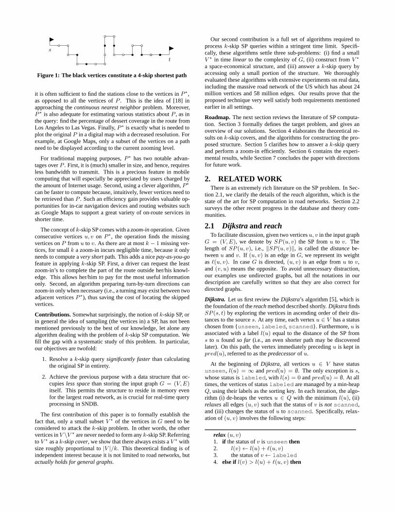
Figure 2: Illustration of reach

5. l(v)← l(u) + (u, v)6. pred(v)← u

The present l(u) is guaranteed to be ‖SP (s, u)‖. The algorithmterminates as soon as t, the destination, is selected by an iteration.

To illustrate, assume that we want to compute SP (s, t) in Fig-ure 2a. In the first iteration, Dijkstra scans s and relaxes (s, a),after which Q = a and l(a) = 1. The next iteration de-heaps aand relaxes (a, b), (a, c). Note that (a, s) is not relaxed because thestatus of s has become scanned. Now Q contains b, c with labels5, 6, respectively. The algorithm then scans b and relaxes (b, d),which labels d with 10. This is followed by de-heaping c, andrelaxing (c, d), (c, e). Note that the relaxation of (c, d) decreasesl(d) to 9. The rest of the algorithm proceeds in the same manner.By tracing the execution, one can verify that, at termination, all thevertices except t have already been scanned.

Dijkstra can be implemented in O(m+n log n) time [3], wheren,m are the number of vertices and edges, respectively (i.e., n =|V |,m = |E|). In a road network, each vertex has an O(1) degree,so the time complexity is essentially O(n log n).

Bi-directional. Dijkstra starts a graph traversal from s and gradu-ally approaches t; call this a forward search. Immediately by sym-metry, the SP problem can also be solved by a backward searchfrom t to s (if G is directed, the backward search implicitly re-verses the direction of each edge). The bi-directional algorithm[10, 20] achieves better efficiency by performing both searches syn-chronously, the effect of which is essentially to explore the verticesu ∈ V in ascending order of rs,t(u), where

rs,t(u) = min‖SP (s, u)‖, ‖SP (u, t)‖. (1)

In fact, if u is closer to s (than to t), then it will first be touched inthe forward search; otherwise, the backward search will find it first.The forward/backward search proceeds as in the standard Dijkstra’salgorithm (as if the other search did not exist). Let Qf (Qb) bethe heap of the forward (backward) direction. Synchronization iscarried out by advancing in each iteration the direction that has asmaller label at the top of the heap.

Bi-directional monitors the distance λ of the shortest s-to-t pathfound so far. λ is set to∞ initially, and may be updated when theforward search (the backward case is symmetric) de-heaps a vertexu whose status in the backward direction is labeled1. Specif-ically, at this time, the algorithm computes λ′ = lf (u) + lb(u),1This status cannot be scanned; otherwise, the algorithm wouldhave terminated right after u was de-heaped by the forward search,as will be clear shortly.

s t

Figure 3: Comparison of Dijkstra, bi-directional, and reach

where lf (u) and lb(u) are the labels of u in the forward and back-ward search, respectively. λ is reduced to λ′ if λ > λ′, sinceit implies the existence of a shorter s-to-t path that concatenatesSP (s, u), (u, v), and SP (v, t), where v is the current predecessorof u in the backward search. The algorithm terminates when eitherdirection de-heaps a vertex already scanned in the other direction.

Let us demonstrate bi-directional on the graph in Figure 2a.After three iterations of each direction, which are the same asin Dijkstra, the forward (backward) search has scanned s, a, b(t, g, f ), such that Qf (Qb) contains vertices c, d (e, d) with la-bels 6, 10, respectively. Currently, λ = ∞. Next, the forwardsearch de-heaps c ∈ Qf and relaxes edges (c, d), (c, e), afterwhich lf (e) = 7, lf (d) = 9. Similarly, the backward search thende-heaps e ∈ Qb. As the status of e in the forward direction islabeled, the algorithm updates λ to lf (e)+ lb(e) = 7+6 = 13,before it relaxes (e, c), (e, d). The forward search continues byde-heaping e ∈ Qf , which, however, has been scanned in thebackward search. The algorithm therefore terminates, without de-heaping d in either direction.

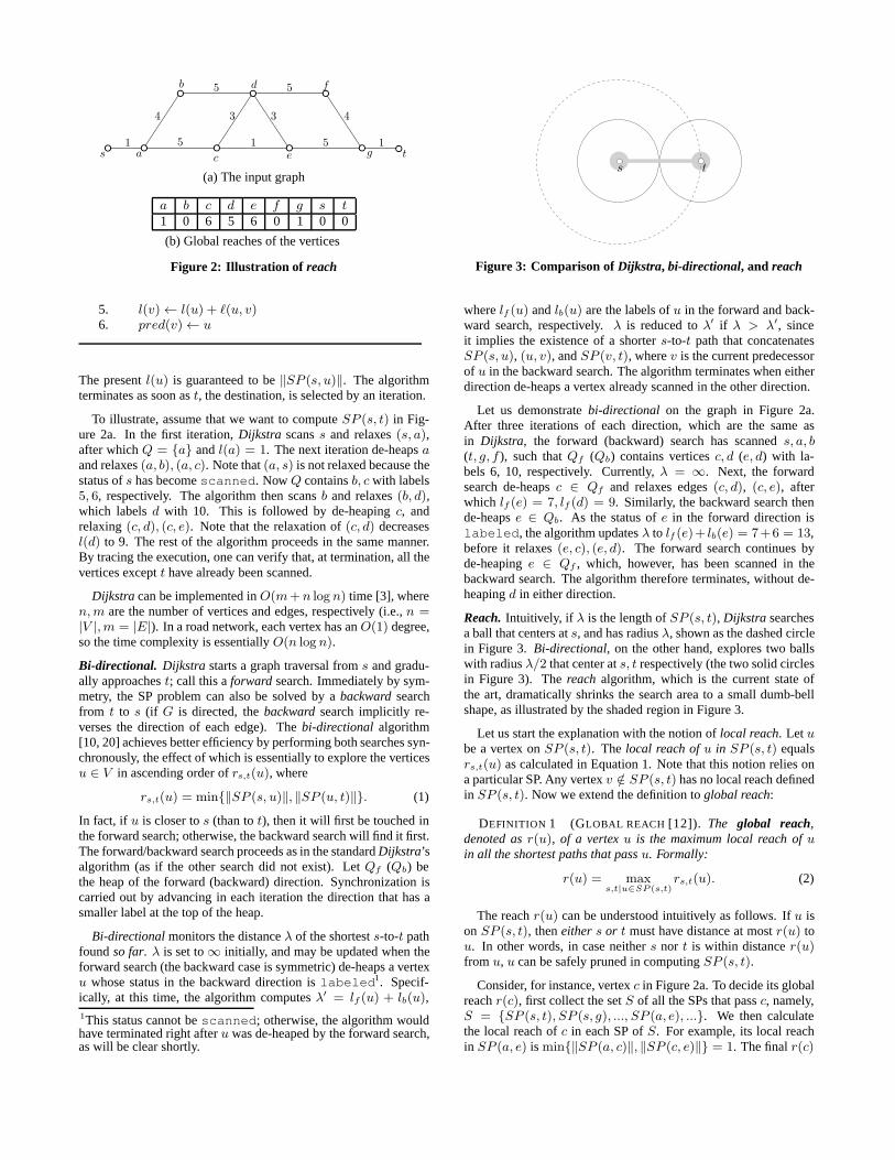
Reach. Intuitively, if λ is the length of SP (s, t), Dijkstra searchesa ball that centers at s, and has radius λ, shown as the dashed circlein Figure 3. Bi-directional, on the other hand, explores two ballswith radius λ/2 that center at s, t respectively (the two solid circlesin Figure 3). The reach algorithm, which is the current state ofthe art, dramatically shrinks the search area to a small dumb-bellshape, as illustrated by the shaded region in Figure 3.

Let us start the explanation with the notion of local reach. Let ube a vertex on SP (s, t). The local reach of u in SP (s, t) equalsrs,t(u) as calculated in Equation 1. Note that this notion relies ona particular SP. Any vertex v /∈ SP (s, t) has no local reach definedin SP (s, t). Now we extend the definition to global reach:

DEFINITION 1 (GLOBAL REACH [12]). The global reach,denoted as r(u), of a vertex u is the maximum local reach of uin all the shortest paths that pass u. Formally:

r(u) = maxs,t|u∈SP (s,t)

rs,t(u). (2)

The reach r(u) can be understood intuitively as follows. If u ison SP (s, t), then either s or t must have distance at most r(u) tou. In other words, in case neither s nor t is within distance r(u)from u, u can be safely pruned in computing SP (s, t).

Consider, for instance, vertex c in Figure 2a. To decide its globalreach r(c), first collect the set S of all the SPs that pass c, namely,S = SP (s, t), SP (s, g), ..., SP (a, e), .... We then calculatethe local reach of c in each SP of S. For example, its local reachin SP (a, e) is min‖SP (a, c)‖, ‖SP (c, e)‖ = 1. The final r(c)

equals the maximum of all the local reaches, which can be verifiedto be 6 (as is its local reach in SP (s, t)). Figure 2b shows theglobal reaches of all the vertices.

In computing SP (s, t), the reach algorithm [10, 12] proceedsin the same way as bi-directional, but may prune a vertex in re-laxing an edge (u, v). Without loss of generality, suppose that therelaxation takes place in the forward search (the backward case issymmetric). This implies that the forward search just scanned u,but has never scanned v (otherwise the edge would not have beenrelaxed). The pruning of reach takes place as follows:

RULE 1. Vertex v is pruned if both of the following hold:

1. v has status labeled or unseen in the backward direction

2. r(v) < lf (u)

where lf (u) is the label of u in the forward search.

In general, reach can be understood as the execution of bi-directional on the vertices that survive pruning. In Figure 2, forexample, reach finds SP (s, t) by scanning only s, a, c, e, g, t. Asin bi-directional, reach first scans s (t) in the forward (backward)direction, after which Qf (Qb) includes a (g) with label 1. Next,the forward search de-heaps a from Qf , and relaxes (a, b), (a, c).The relaxation of (a, b) prunes b by Rule 1 because r(b) = 0 <lf (a) = 1. The backward search then eliminates f in a similarfashion. The rest of the algorithm proceeds as in bi-directional.Vertex d does not need to be scanned for the reason explained ear-lier for bi-directional.

The space consumption of reach is very economical because, ex-cept G itself, only one extra value needs to be stored for each ver-tex. However, it can be expensive to calculate the exact reach ofevery vertex. Fortunately, there are fast algorithms [10, 12] to ob-tain approximate reaches that are guaranteed to upper bound theiroriginal values. Pruning remains the same except that r(u) shouldbe replaced by its upper bound. The outstanding efficiency of thisalgorithm on road networks has been theoretically justified [1].

2.2 More results on SP computationThe A algorithm [13] is a classic SP solution that captures Dijk-

stra as a special case. The effectiveness of A relies on a method tocalculate, typically in constant time, a lower bound of ‖SP (u, v)‖for any two vertices u, v. Apparently, 0 can be a trivial lowerbound, but in that case A degenerates into Dijkstra. In general,the tighter the lower bounds are, the faster A is than Dijkstra.

Motivated by this, Agrawal and Jagadish [2] proposed to pre-compute the distances between each vertex and a special set of ver-tices called landmarks. In answering a SP query, those distancesare deployed to derive lower bounds based on triangle inequality.This idea is also the basis of the ALT algorithm developed by Gold-berg and Harrelson [9], which has lower query time (than [2]) atthe tradeoff of consuming more space. The experiments of [10]indicate that ALT is slower than the reach method described in Sec-tion 2.1. Note, however, that ALT and reach are compatible, in thesense that their heuristics can be applied at the same time to maxi-mize efficiency [10].

Sanders and Schultes [8, 25, 26] presented a highway hierar-chy (HH) technique, whose rationale is to identify some edges thatmimic the role of highways in reality. In computing a SP, the algo-rithm of HH modifies Dijkstra so that the search can skip as manynon-highway edges as possible, and thus, terminate earlier. Based

on the empirical evaluation of [10, 25], HH has comparable perfor-mance with respect to reach.

The separator technique is another popular approach [15, 16,17] to preprocess a graph G for efficient SP retrieval. The idea is todivide the vertices of G into several components, and for each com-ponent, extract a set of boundary vertices such that the SP betweentwo vertices in different components must go through a boundaryvertex. Query efficiency benefits from the fact that, most computa-tion of a SP can be restricted only to the boundary vertices. Accord-ing to [25], however, separator-based methods are not as efficient asHH on road networks. Another disadvantage is that these methodsoften have expensive space consumption. For example, the spaceof [15] is at the order of n1.5 (where n is the number of vertices),which is prohibitive for massive graphs.

In [28], Wagner et al. described a geometric container technique,which associates each edge (u, v) in G with a geometric region.The region covers all the vertices t such that the SP from u to tgoes through v. In running Dijkstra, such regions can be used toprune many vertices that do not appear in the SP. Lauther [19] in-tegrated a similar idea with the bi-directional algorithm discussedin Section 2.1. Samet et al. [24] proposed to break the geometricregions into smaller disjoint pieces that can be indexed by a quad-tree. Their solution lowers the cost of SP calculation (compared to[19, 28]), but entails O(n1.5) space. A common shortcoming of[19, 24, 28] is that their preprocessing essentially determines theSPs between all pairs of vertices. The all-SP problem is notori-ously difficult. Even on planar graphs, the fastest solution requiresO(n2) time [7], which is practically intractable for large n.

Recently, Sankaranarayanan et al. [27] proposed a path oraclethat is constructed from well-separated pair decomposition, andcan be used to accelerate SP retrieval. Such an oracle consumesO(s2n) space in 2-d space, where s is shown to be around 12 forpractical data. Xiao et al. [30] showed that SP queries can be accel-erated by exploiting symmetry in the data graph. Their approach,however, is limited to the case where all edges have a unit weight.Wei [29] developed an alternative solution by resorting to tree de-composition [23]. Rice and Tsotras [22] studied the shortest pathproblem with label restrictions. Some other work considers how toestimate shortest path distances, e.g., [11, 21].

We emphasize that all the works aforementioned calculate tradi-tional, complete, SPs. The concept of k-skip SP has not appearedpreviously, and is formalized in the next section for the first time inthe literature.

3. K-SKIP SHORTEST PATHSFor simplicity, we assume that the data graph G = (V,E) is

undirected, and will discuss directed graphs only when the exten-sion is not straightforward. The following definition formalizes k-skip SP:

DEFINITION 2 (k-SKIP SHORTEST PATH). Let SP (s, t) bethe shortest path from source s to destination t. Label the ver-tices in SP (s, t) in the order they appear: v1, v2, ..., vl (i.e.,v1 = s, vl = t), where l is the total number of vertices in thepath. If l ≥ k, let P be an ordered subset of v1, ..., vl, wherethe ordering respects that in SP (s, t). P is a k-skip shortest pathfrom s to t if

P ∩ vi, ..., vi+k−1 = ∅ (3)

for every 1 ≤ i ≤ l − k + 1.

a

b

c

d

e

f

a

b

c

d

e

f

.

.

3

33

3

33

2

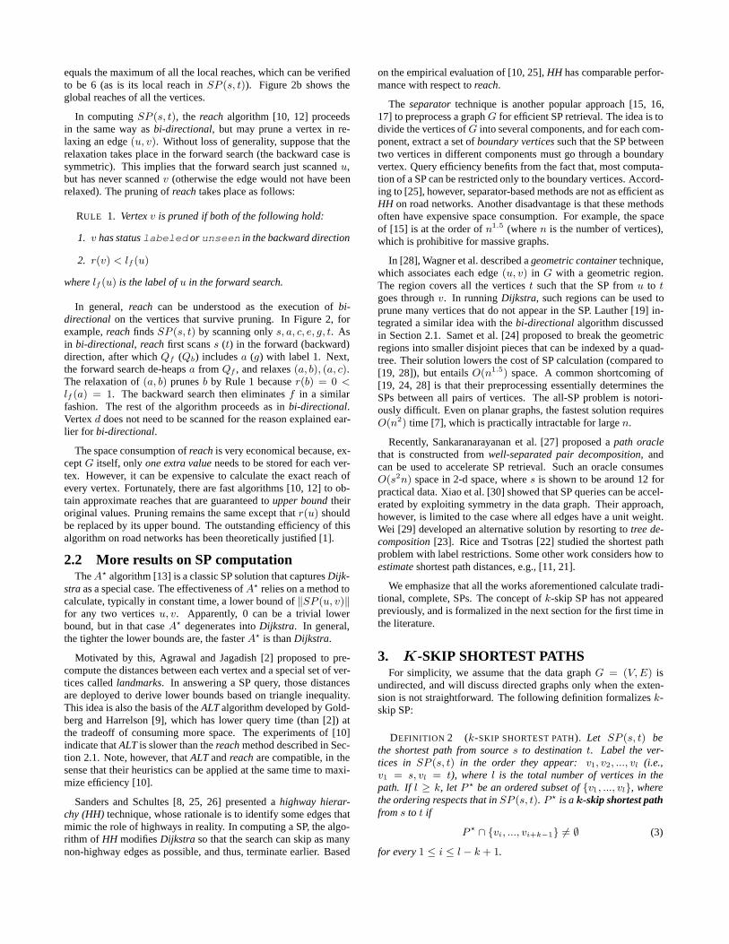
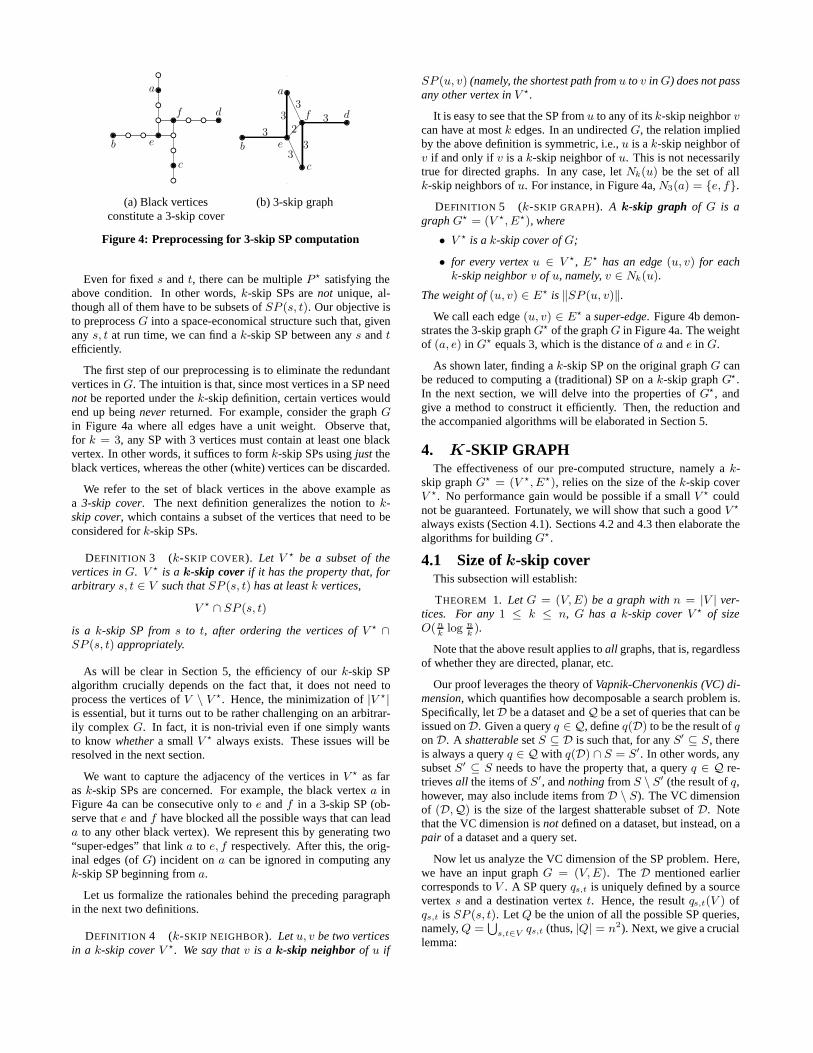
(a) Black vertices (b) 3-skip graphconstitute a 3-skip cover

Figure 4: Preprocessing for 3-skip SP computation

Even for fixed s and t, there can be multiple P satisfying theabove condition. In other words, k-skip SPs are not unique, al-though all of them have to be subsets of SP (s, t). Our objective isto preprocess G into a space-economical structure such that, givenany s, t at run time, we can find a k-skip SP between any s and tefficiently.

The first step of our preprocessing is to eliminate the redundantvertices in G. The intuition is that, since most vertices in a SP neednot be reported under the k-skip definition, certain vertices wouldend up being never returned. For example, consider the graph Gin Figure 4a where all edges have a unit weight. Observe that,for k = 3, any SP with 3 vertices must contain at least one blackvertex. In other words, it suffices to form k-skip SPs using just theblack vertices, whereas the other (white) vertices can be discarded.

We refer to the set of black vertices in the above example asa 3-skip cover. The next definition generalizes the notion to k-skip cover, which contains a subset of the vertices that need to beconsidered for k-skip SPs.

DEFINITION 3 (k-SKIP COVER). Let V be a subset of thevertices in G. V is a k-skip cover if it has the property that, forarbitrary s, t ∈ V such that SP (s, t) has at least k vertices,

V ∩ SP (s, t)

is a k-skip SP from s to t, after ordering the vertices of V ∩SP (s, t) appropriately.

As will be clear in Section 5, the efficiency of our k-skip SPalgorithm crucially depends on the fact that, it does not need toprocess the vertices of V \ V . Hence, the minimization of |V |is essential, but it turns out to be rather challenging on an arbitrar-ily complex G. In fact, it is non-trivial even if one simply wantsto know whether a small V always exists. These issues will beresolved in the next section.

We want to capture the adjacency of the vertices in V as faras k-skip SPs are concerned. For example, the black vertex a inFigure 4a can be consecutive only to e and f in a 3-skip SP (ob-serve that e and f have blocked all the possible ways that can leada to any other black vertex). We represent this by generating two“super-edges” that link a to e, f respectively. After this, the orig-inal edges (of G) incident on a can be ignored in computing anyk-skip SP beginning from a.

Let us formalize the rationales behind the preceding paragraphin the next two definitions.

DEFINITION 4 (k-SKIP NEIGHBOR). Let u, v be two verticesin a k-skip cover V . We say that v is a k-skip neighbor of u if

SP (u, v) (namely, the shortest path from u to v in G) does not passany other vertex in V .

It is easy to see that the SP from u to any of its k-skip neighbor vcan have at most k edges. In an undirected G, the relation impliedby the above definition is symmetric, i.e., u is a k-skip neighbor ofv if and only if v is a k-skip neighbor of u. This is not necessarilytrue for directed graphs. In any case, let Nk(u) be the set of allk-skip neighbors of u. For instance, in Figure 4a, N3(a) = e, f.

DEFINITION 5 (k-SKIP GRAPH). A k-skip graph of G is agraph G = (V , E), where

• V is a k-skip cover of G;

• for every vertex u ∈ V , E has an edge (u, v) for eachk-skip neighbor v of u, namely, v ∈ Nk(u).

The weight of (u, v) ∈ E is ‖SP (u, v)‖.We call each edge (u, v) ∈ E a super-edge. Figure 4b demon-

strates the 3-skip graph G of the graph G in Figure 4a. The weightof (a, e) in G equals 3, which is the distance of a and e in G.

As shown later, finding a k-skip SP on the original graph G canbe reduced to computing a (traditional) SP on a k-skip graph G.In the next section, we will delve into the properties of G, andgive a method to construct it efficiently. Then, the reduction andthe accompanied algorithms will be elaborated in Section 5.

4. K-SKIP GRAPHThe effectiveness of our pre-computed structure, namely a k-

skip graph G = (V , E), relies on the size of the k-skip coverV . No performance gain would be possible if a small V couldnot be guaranteed. Fortunately, we will show that such a good V

always exists (Section 4.1). Sections 4.2 and 4.3 then elaborate thealgorithms for building G.

4.1 Size of k-skip coverThis subsection will establish:

THEOREM 1. Let G = (V,E) be a graph with n = |V | ver-tices. For any 1 ≤ k ≤ n, G has a k-skip cover V of sizeO(n

klog n

k).

Note that the above result applies to all graphs, that is, regardlessof whether they are directed, planar, etc.

Our proof leverages the theory of Vapnik-Chervonenkis (VC) di-mension, which quantifies how decomposable a search problem is.Specifically, letD be a dataset andQ be a set of queries that can beissued onD. Given a query q ∈ Q, define q(D) to be the result of qon D. A shatterable set S ⊆ D is such that, for any S′ ⊆ S, thereis always a query q ∈ Q with q(D) ∩ S = S′. In other words, anysubset S′ ⊆ S needs to have the property that, a query q ∈ Q re-trieves all the items of S′, and nothing from S \ S′ (the result of q,however, may also include items from D \ S). The VC dimensionof (D,Q) is the size of the largest shatterable subset of D. Notethat the VC dimension is not defined on a dataset, but instead, on apair of a dataset and a query set.

Now let us analyze the VC dimension of the SP problem. Here,we have an input graph G = (V,E). The D mentioned earliercorresponds to V . A SP query qs,t is uniquely defined by a sourcevertex s and a destination vertex t. Hence, the result qs,t(V ) ofqs,t is SP (s, t). Let Q be the union of all the possible SP queries,namely, Q =

⋃s,t∈V qs,t (thus, |Q| = n2). Next, we give a crucial

lemma:

LEMMA 1. For any graph G, the VC dimension of (V,Q) is 2.

PROOF. Assume for contradiction that the VC dimension d of(V,Q) is at least 3 (note that d must be an integer). Hence, there isa shatterable set S with size d, which belongs to the SP returned bya query q ∈ Q. Let u1, u2, ..., ud be the vertices of S ordered bytheir appearance on the SP. Hence, u2 is on the SP from u1 to ud.In this case, however, S′ = u1, ud cannot be in any SP that doesnot contain u2, contradicting the fact that S is shatterable.

It remains to verify that the VC dimension can be 2. We omit thedetails as this is trivial.

The rest of the proof (for Theorem 1) concerns ε-net. Let D,Qbe as defined earlier in our introduction to VC dimension. A setS ⊆ D is an ε-net of (D,Q) if S ∩ q(D) = ∅ for any q satisfying|q(D)| ≥ ε|D|. In other words, if q retrieves no less than ε|D|items, at least one of these items must appear in S. The lemmabelow draws the correspondence between ε-net and k-skip cover:

LEMMA 2. A ( kn)-net V of (V,Q) is a k-skip cover of G.

PROOF. Let Q′ be the set of queries q ∈ Q such that the SPq(V ) returned by q has exactly k vertices. By the definition of(k/n)-net, for each q′ ∈ Q′, V ∩ q′(V ) = ∅. Now consider aquery q ∈ Q \ Q′ whose result q(V ) has more than k vertices.Clearly, any sub-path of q(V ) including k vertices is the resultq′(v) of some q′ ∈ Q′, from which V contains at least a vertex.Therefore, V is a k-skip cover.

The ε-net theorem [14] dictates that any (D,Q) with VC dimen-sion d has an ε-net of size O(d

εlog 1

ε). This, combined with Lem-

mas 1 and 2, gives Theorem 1.

Remark 1. Effectively, the proof of the ε-net theorem [14] showsthat a random subset of D with size O(d

εlog 1

ε) is an ε-net with

high probability. Hence, we can find a k-skip cover V by simplytaking O(n

klog n

k) vertices from V randomly.

Remark 2. There is a trivial lower bound of n/k on the size of a k-skip cover. Hence, the upper bound in Theorem 1 is asymptoticallytight, up to only a logarithmic factor.

4.2 Computing a k-skip coverAs mentioned in the previous subsection, a k-skip cover V can

be obtained by taking O(nklog n

k) random vertices from V . It is

well-known that randomized techniques generally work much bet-ter in practice than predicted by theory. Therefore, the V of areal graph would be much smaller, rendering a sample set of sizeO(n

klog n

k) most probably unnecessarily large. Of course, we

could artificially reduce the number of samples, but a good sam-ple size appears to be difficult to decide. A large size gives onlymarginal improvement, whereas a small size has the risk that thesample set may no longer be a k-skip cover.

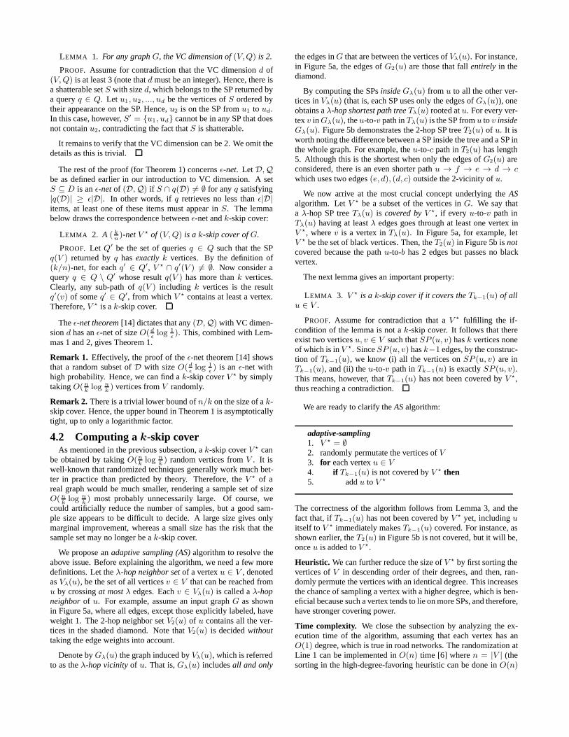
We propose an adaptive sampling (AS) algorithm to resolve theabove issue. Before explaining the algorithm, we need a few moredefinitions. Let the λ-hop neighbor set of a vertex u ∈ V , denotedas Vλ(u), be the set of all vertices v ∈ V that can be reached fromu by crossing at most λ edges. Each v ∈ Vλ(u) is called a λ-hopneighbor of u. For example, assume an input graph G as shownin Figure 5a, where all edges, except those explicitly labeled, haveweight 1. The 2-hop neighbor set V2(u) of u contains all the ver-tices in the shaded diamond. Note that V2(u) is decided withouttaking the edge weights into account.

Denote by Gλ(u) the graph induced by Vλ(u), which is referredto as the λ-hop vicinity of u. That is, Gλ(u) includes all and only

the edges in G that are between the vertices of Vλ(u). For instance,in Figure 5a, the edges of G2(u) are those that fall entirely in thediamond.

By computing the SPs inside Gλ(u) from u to all the other ver-tices in Vλ(u) (that is, each SP uses only the edges of Gλ(u)), oneobtains a λ-hop shortest path tree Tλ(u) rooted at u. For every ver-tex v inGλ(u), the u-to-v path in Tλ(u) is the SP from u to v insideGλ(u). Figure 5b demonstrates the 2-hop SP tree T2(u) of u. It isworth noting the difference between a SP inside the tree and a SP inthe whole graph. For example, the u-to-c path in T2(u) has length5. Although this is the shortest when only the edges of G2(u) areconsidered, there is an even shorter path u → f → e → d → cwhich uses two edges (e, d), (d, c) outside the 2-vicinity of u.

We now arrive at the most crucial concept underlying the ASalgorithm. Let V be a subset of the vertices in G. We say thata λ-hop SP tree Tλ(u) is covered by V , if every u-to-v path inTλ(u) having at least λ edges goes through at least one vertex inV , where v is a vertex in Tλ(u). In Figure 5a, for example, letV be the set of black vertices. Then, the T2(u) in Figure 5b is notcovered because the path u-to-b has 2 edges but passes no blackvertex.

The next lemma gives an important property:

LEMMA 3. V is a k-skip cover if it covers the Tk−1(u) of allu ∈ V .

PROOF. Assume for contradiction that a V fulfilling the if-condition of the lemma is not a k-skip cover. It follows that thereexist two vertices u, v ∈ V such that SP (u, v) has k vertices noneof which is in V . Since SP (u, v) has k−1 edges, by the construc-tion of Tk−1(u), we know (i) all the vertices on SP (u, v) are inTk−1(u), and (ii) the u-to-v path in Tk−1(u) is exactly SP (u, v).This means, however, that Tk−1(u) has not been covered by V ,thus reaching a contradiction.

We are ready to clarify the AS algorithm:

adaptive-sampling1. V = ∅2. randomly permutate the vertices of V3. for each vertex u ∈ V4. if Tk−1(u) is not covered by V then5. add u to V

The correctness of the algorithm follows from Lemma 3, and thefact that, if Tk−1(u) has not been covered by V yet, including uitself to V immediately makes Tk−1(u) covered. For instance, asshown earlier, the T2(u) in Figure 5b is not covered, but it will be,once u is added to V .

Heuristic. We can further reduce the size of V by first sorting thevertices of V in descending order of their degrees, and then, ran-domly permute the vertices with an identical degree. This increasesthe chance of sampling a vertex with a higher degree, which is ben-eficial because such a vertex tends to lie on more SPs, and therefore,have stronger covering power.

Time complexity. We close the subsection by analyzing the ex-ecution time of the algorithm, assuming that each vertex has anO(1) degree, which is true in road networks. The randomization atLine 1 can be implemented in O(n) time [6] where n = |V | (thesorting in the high-degree-favoring heuristic can be done in O(n)

4

52

22

2

2

2

2

2

2u a

b

e

c

d

f2

.

.

u a

b

e

cf2

(a) 2-hop vicinity of u and its (b) 2-hop SP tree of u

Figure 5: Deciding whether to sample u into a 3-skip cover

time when there are only a constant number of possible degrees).The λ-hop vicinity of a node u can be found by a standard breathfirst traversal (BFT) initiated at u, which terminates in O(σλ(u))time where σλ(u) is the number of λ-hop neighbors of u, i.e.,σλ(u) = |Vλ(u)|. Then, the λ-hop SP tree Tλ(u) can be extractedfrom Gλ(u) using the Dijkstra’s algorithm in O(σλ(u) log σλ(u))time. Checking whether Tλ(u) is covered by V demands a sin-gle traversal of Tλ(u) in O(σλ(u)) time. Hence, the total cost ofthe algorithm is O(nσk−1 log σk−1), where σk−1 is the averagenumber of (k − 1)-hop neighbors of the vertices in V .

The value of σk−1 depends on the structure of the road network,but not the number n of the vertices. For example, consider twosimple road networks that are a 100 × 100 and 1000 × 1000 grid,respectively. Although the second grid has 100 times more vertices,the two grids have the same σk−1 = Θ(k2). Hence, when k is farsmaller than n, O(nσk−1 log σk−1) grows linearly with n.

4.3 Computing a k-skip graphRecall that the goal of our preprocessing is to produce a k-skip

graph G = (V , E). V is simply a k-skip cover, whose deriva-tion has been clarified in Section 4.2. Next we complete the puzzleby explaining the derivation of E. Our discussion concentrateson the subproblem that, given a vertex u ∈ V , how to calculatethe set Nk(u) of its k-skip neighbors (Definition 4). Once this isdone, it is trivial to obtain E according to Definition 5, because weonly need to add to E a super-edge from each u to every vertexv ∈ Nk(u).

We will call each vertex of V a sample from now on, due to thesampling nature of the AS algorithm. A naive approach to acquireNk(u) is to first find the SP from u to every other sample v ∈V , and then add v to Nk(u) if the path passes no other sample.However, since |V | ≥ n/k (see Remark 2 of Section 4.1), doingso for all u ∈ V would incur Ω(n2/k) time, which is prohibitivefor large n. We circumvent the performance pitfall by aiming ata superset Mk(u) of Nk(u). As will be clear shortly, despite thatMk(u) may result in a G with more edges, it has the advantageof being computable in significantly less time, thus allowing ourtechnique to support gigantic graphs.

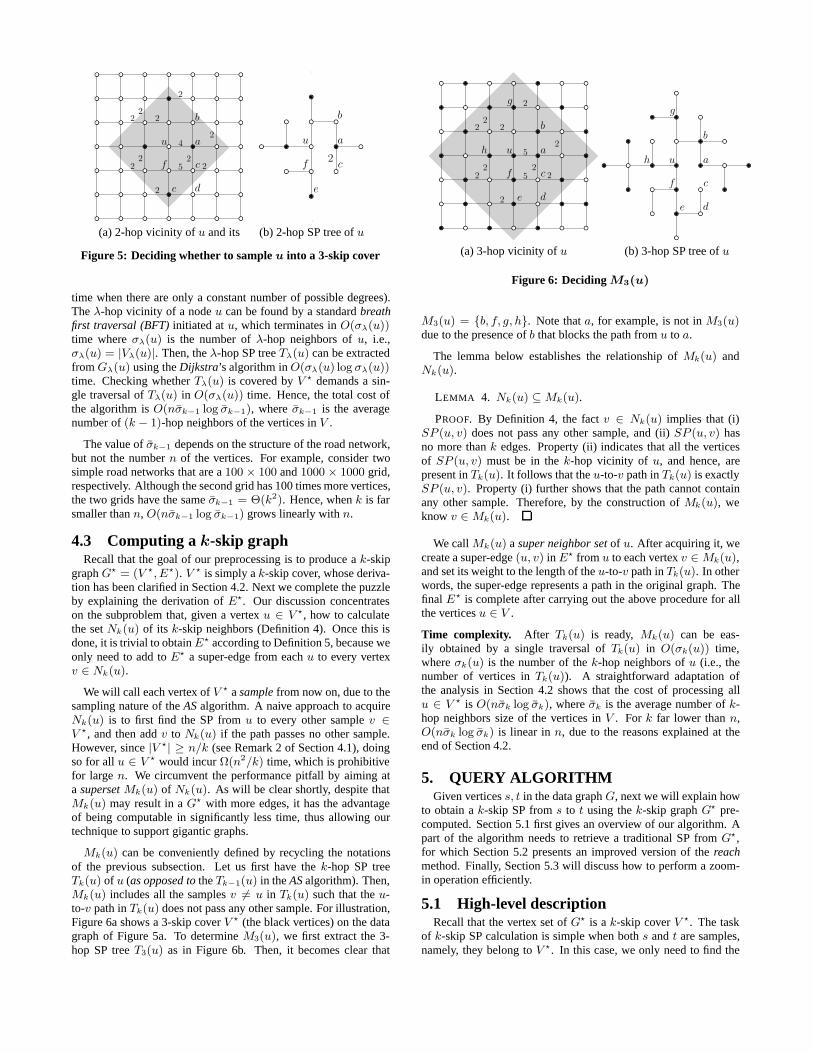
Mk(u) can be conveniently defined by recycling the notationsof the previous subsection. Let us first have the k-hop SP treeTk(u) of u (as opposed to the Tk−1(u) in the AS algorithm). Then,Mk(u) includes all the samples v = u in Tk(u) such that the u-to-v path in Tk(u) does not pass any other sample. For illustration,Figure 6a shows a 3-skip cover V (the black vertices) on the datagraph of Figure 5a. To determine M3(u), we first extract the 3-hop SP tree T3(u) as in Figure 6b. Then, it becomes clear that

u a

b

e

c

d

f

g

h 5

52

22

2

2

2

2

2

2

2u a

b

e

c

d

f

g

h

(a) 3-hop vicinity of u (b) 3-hop SP tree of u

Figure 6: Deciding M3(u)

M3(u) = b, f, g, h. Note that a, for example, is not in M3(u)due to the presence of b that blocks the path from u to a.

The lemma below establishes the relationship of Mk(u) andNk(u).

LEMMA 4. Nk(u) ⊆Mk(u).

PROOF. By Definition 4, the fact v ∈ Nk(u) implies that (i)SP (u, v) does not pass any other sample, and (ii) SP (u, v) hasno more than k edges. Property (ii) indicates that all the verticesof SP (u, v) must be in the k-hop vicinity of u, and hence, arepresent in Tk(u). It follows that the u-to-v path in Tk(u) is exactlySP (u, v). Property (i) further shows that the path cannot containany other sample. Therefore, by the construction of Mk(u), weknow v ∈Mk(u).

We call Mk(u) a super neighbor set of u. After acquiring it, wecreate a super-edge (u, v) in E from u to each vertex v ∈Mk(u),and set its weight to the length of the u-to-v path in Tk(u). In otherwords, the super-edge represents a path in the original graph. Thefinal E is complete after carrying out the above procedure for allthe vertices u ∈ V .

Time complexity. After Tk(u) is ready, Mk(u) can be eas-ily obtained by a single traversal of Tk(u) in O(σk(u)) time,where σk(u) is the number of the k-hop neighbors of u (i.e., thenumber of vertices in Tk(u)). A straightforward adaptation ofthe analysis in Section 4.2 shows that the cost of processing allu ∈ V is O(nσk log σk), where σk is the average number of k-hop neighbors size of the vertices in V . For k far lower than n,O(nσk log σk) is linear in n, due to the reasons explained at theend of Section 4.2.

5. QUERY ALGORITHMGiven vertices s, t in the data graph G, next we will explain how

to obtain a k-skip SP from s to t using the k-skip graph G pre-computed. Section 5.1 first gives an overview of our algorithm. Apart of the algorithm needs to retrieve a traditional SP from G,for which Section 5.2 presents an improved version of the reachmethod. Finally, Section 5.3 will discuss how to perform a zoom-in operation efficiently.

5.1 High-level descriptionRecall that the vertex set of G is a k-skip cover V . The task

of k-skip SP calculation is simple when both s and t are samples,namely, they belong to V . In this case, we only need to find the

s t

Mk(t)Mk(s)

G

Figure 7: In-place sampling of s and t

SP from s to t in G, that is, traveling only on the super-edges. Bythe definition of G, this SP is guaranteed to be a k-skip SP in theoriginal graph G.

Let us focus on the situation where neither s nor t is a sample.Our solution is to sample them into G right away, so that the casecan be converted to the previous scenario where s and t are sam-ples. The inclusion of s, t as samples is temporary; after queryprocessing, they will be removed from G, whose size thereforedoes not change.

Incorporation of s, t in G involves two steps. First, s and tare inserted in V . Second, some super-edges are created to re-flect the appearance of s, t, in the same way the existing super-edges are computed. That is, given s (similarly for t), we firstobtain the super neighbor set Mk(s) of s, and then add to E

a super-edge from s to each u ∈ Mk(s), all exactly as de-scribed in Section 4.3. This process is illustrated in Figure 7.The analysis of Section 4.3 shows that, the above strategy runs inO(σs(k) log σs(k)+σt(k) log σt(k)) time. Remember that σs(k),the number of k-hop neighbors of s, is low when k is small (simi-larly for σt(k)). Hence, sampling-in-place s and t incurs insignifi-cant overhead.

Let Gs,t be the resulting G with the new super-edges, and

SP (s, t) be the SP from s to t on G. The rest of our algorithm re-turns directly SP (s, t), whose correctness is shown in the lemmabelow:

LEMMA 5. SP (s, t) is a k-skip SP of SP (s, t).

PROOF. Let u be the first sample (counting also t) when wewalk from s along SP (s, t). By the definition of k-skip SP,SP (s, u) has at most k edges, all of which appear in the k-hopSP tree of s. Hence, u ∈ Mk(s) (otherwise, there would be an-other sample on SP (s, u), contradicting the choice of u), whichmeans (s, u) is a super-edge in G

s,t.

Let v be the last sample (counting also s) on SP (s, t) before wearrive at t. A similar argument shows that (v, t) is also a super-edge. The correctness of the lemma then follows from the fact thatevery super-edge has a weight equal to the length of the path itrepresents.

Remark on directed graphs. Let S be the set of super-edges on tnewly computed for G

s,t. In the above, we computed S by firstfinding the super neighbor set Mk(t) of t, and then inserting asuper-edge (u, t) for each u ∈ Mk(t). If G is directed, the deriva-tion of S is slightly different, in the sense that we need to firstreverse the directions of the edges in G, before proceeding as de-scribed earlier. Intuitively, Mk(t) should contain the samples thatcan reach t “directly” (without passing another sample). Reversingdirections allows us to apply the same algorithm in Section 4.2 toextract Mk(t), originally designed to find samples reachable fromt directly. The reversing incurs no additional execution time, be-

u va b c d e

24510423

Figure 8: Super reach calculation

cause a direction change can take place only when the relevant edgeis touched by the algorithm.

5.2 Reach

Now that we have converted k-skip SP computation to findingSP (s, t) on G (in case s, t are not samples, simply treat G

s,t

as G), many SP algorithms such as Dijkstra, bi-directional, andreach, can be plugged in to obtain SP(s, t). However, as thosemethods are not designed for our context, they may be improvedby taking into account the characteristics of G. Next, we achievethe purpose for reach.

As discussed in Section 2.1, reach prunes a vertex v in relaxingan edge (u, v), if the global reach r(v) of v is small, compared tothe distance that the algorithm has traveled in the forward/backwardsearch (see Rule 1). On a k-skip graph, using only r(v) for pruningmay miss plenty of pruning opportunities. The reason is that, asuper-edge (u, v) implicitly captures a path in the original graph,and hence, can be pruned as long as any vertex on that path has alow global reach. Motivated by this, we formulate a new notion:

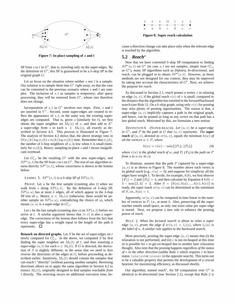
DEFINITION 6 (SUPER REACH). Let (u, v) be a super-edgein G, and P be the path in G that (u, v) represents. The superreach of (u, v), denoted as sr(u, v), equals the minimum h(w) ofall the vertices w ∈ P , where

h(w) = r(w)−min‖P1‖, ‖P2‖ (4)

where r(w) is the global reach of w, and P1 (P2) is the path on Pfrom u to w (w to v).

To illustrate, assume that the path P captured by a super-edge(u, v) is as shown in Figure 8. The number above each vertex isits global reach (e.g., r(u) = 3); and suppose for simplicity all theedges have weight 1. To decide, for example, h(b), we first observe‖P1‖ = 2 and ‖P2‖ = 4, and then calculate by Equation 4 h(b) =4 − min2, 4 = 2. After S = h(u), h(a), ..., h(e), h(v) isready, the super reach sr(u, v) can be determined as the minimumof S, i.e., h(a) = 1.

Apparently, sr(u, v) can be computed in time linear to the num-ber of vertices in P , i.e., at most k. Also, preserving all the superreaches entails small space, as only one extra value per super edgeis stored. Next, we propose a new rule to enhance the pruningpower of reach.

RULE 2. When the forward search is about to relax a superedge (u, v), prune the edge if sr(u, v) < lf (u), where lf (u) isthe label of u. A similar rule applies to the backward search.

More precisely, pruning the super-edge (u, v) means that (i) therelaxation is not performed, and (ii) v is not en-heaped at this time(it is possible for v to get en-heaped due to another later relaxationthough). Also note that the pruning happens regardless of the statusof v in the other direction (unlike Rule 1 which requires v to havestatus labeled or unseen in the opposite search). This turns outto be a valuable property that permits the development of a crucialheuristic for maximizing efficiency, as discussed shortly.

Our algorithm, named reach, for SP computation over G isidentical to bi-directional (see Section 2.1), except that Rule 2 is

checked prior to every edge relaxation in an attempt to avoid therelaxation. The following theorem establishes the correctness ofthe algorithm.

THEOREM 2. Reach finds a SP on G correctly.

PROOF. If the forward or backward search applies Rule 2 toprune a super-edge on SP(s, t), we say that a blow occurs. Thelemma is obvious if no blow ever happens, so the subsequent dis-cussion considers that there was at least one blow. Our argumentproceeds in two steps. First, we will show that there can be onlyone blow during the execution of reach. This implies that everysuper-edge in SP(s, t) must be eventually relaxed in at least onedirection, since two blows are needed to eliminate a super-edgefrom both directions. Equipped with these facts, we will prove thelemma in the second step.

Step 1. Without loss of generality, assume that the first blow oc-curred in the forward search, and eliminated super-edge (u, v) ∈SP (s, t). It is easy to see that, when the blow happened, (i) theforward direction had scanned all the vertices in SP∗(s, u), and (ii)sr(u, v) < lf (u) (by Rule 2), where lf (u) equals ‖SP (s, u)‖ =‖SP (s, u)‖. Thus,

sr(u, v) < ‖SP (s, u)‖. (5)

Let P be the path in G that (u, v) represents, and w be the vertex inP that minimizes h(w) (see Equation 4), i.e., sr(u, v) = r(w) −min‖SP (u, w)‖, ‖SP (w, v)‖. Hence,

r(w)− ‖SP (u, w)‖ ≤ sr(u, v) (6)

r(w)− ‖SP (w, v)‖ ≤ sr(u, v). (7)

Inequalities 5 and 6 lead to r(w) < ‖SP (s, u)‖ +‖SP (u, w)‖ = ‖SP (s, w)‖. By definition, r(w) is atleast min‖SP (s, w)‖, ‖SP (w, t)‖. So we know r(w) ≥‖SP (w, t)‖ which, together with Inequality 7, gives:

sr(u, v) ≥ ‖SP (w, t)‖ − ‖SP (w, v)‖ = ‖SP (v, t)‖. (8)

Inequalities 5 and 8 indicate ‖SP (s, u)‖ > ‖SP (v, t)‖. Due to(i) the way bi-directional synchronizes the two directions and (ii)the choice of (u, v), the backward search must have scanned all thevertices on SP (v, t) before the blow happened.

If there was a second blow, either the forward search needed tode-heap a vertex in SP (v, t), or the reverse search needed to de-heap a vertex in SP (s, u). But both events would have terminatedthe algorithm immediately, because bi-direction ends when the for-ward/backward search de-heaps a vertex already scanned in theother direction. Therefore, no second blow could have occurred.

Step 2. The analysis of Step 1 shows that, at the moment the blowtook place, the status of v was scanned in the backward search.This means that, u had a status of labeled in the backward di-rection. Consequently, when the forward search de-heaped u (rightbefore the blow), as in bi-directional, reach updated λ, whichrecords the length of the SP found so far, to lf (u) + lb(u) =‖SP (s, u)‖ + ‖SP (u, t)‖ = ‖SP (s, t)‖. In other words,reach found the correct SP successfully.

After the forward (or backward) search de-heaps a vertex u, ourcurrent reach attempts to prune each out-going super-edge at uwith Rule 2. Hence, the rule has to be applied numerous timesif many super-edges out of u can be eliminated. This can harmthe efficiency because each vertex in G may have a large degree(unlike G, where each vertex’s degree is bounded), the result of

which is that we may end up applying the rule a huge number oftimes during the entire algorithm.

The next heuristic allows us to significantly reduce the cost,while still eliminating as many super-edges as before, with no in-crease in the space assumption at all. The idea is to store the outgo-ing super-edges of each vertex u in G in descending order of theirsuper reaches. After de-heaping u in the algorithm, we attemptto prune those edges in the sorted order. The benefit is that oncean edge has been eliminated by Rule 2, we can assert that all theremaining edges can be pruned as well, because all of them musthave lower super reaches (than the one pruned), and therefore, willsatisfy Rule 2 for sure.

The above heuristic is made possible by the fact that, to prune anedge (u, v), Rule 2 does not require checking the status of v (in thesearch opposite to the one where the pruning happens). If this wasnot the case, the heuristic would virtually promise no performancegain as checking the status of v takes nearly the same amount oftime as applying Rule 2 on (u, v).

Remark. It is worth pointing out that, the mechanism behindreach, namely the integration of bi-directional and the no-status-checking pruning strategy of Rule 2, actually extends the algorith-mic paradigm for SP computation as illustrated in Section 2.1. Inretrospect, reach is an immediate benefit of this extension.

5.3 Zoom-inAs mentioned in Section 1, the concept of k-skip SP is naturally

accompanied by a zoom-in operator. Given consecutive verticesu, v on a k-skip SP (s, t), the operator finds all the vertices be-tween u and v on the full SP (s, t). A naive way to zoom-in is torun Dijkstra to extract the SP from u to v. A faster solution ap-plies bi-directional. In fact, one can do even better using reach.However, simply executing reach afresh to compute SP (u, v) isnot likely to outperform bi-directional much. This is because thepruning of reach (i.e., Rule 1 in Section 2.1) is effective only if thevertex u de-heaped in the, for example, forward search has a largelabel lf (u). This requires the forward search to have come a longway from the source, a situation that will not happen between u andv, because they are at most k vertices apart on their SP.

There is a simple remedy to significantly boost the efficiency.The main idea is to pretend as if we were running reach to computeSP (s, t) (as opposed to SP (u, v)), and that the algorithm had justcome to u and v in the forward and backward searches, respec-tively. We “continue” the forward direction by setting lf (u) =min‖SP (s, u)‖, ‖SP (v, t)‖, and making u the only vertex inthe heap Qf (which implies giving u the status labeled). Notethat both ‖SP (s, u)‖ and ‖SP (v, t)‖ are available in the k-skipSP (s, t) already calculated. Similarly, the backward direction isalso continued by setting lb(v) = lf (u) and creating a heap Qb

with only v inside. We then start a normal iteration and proceed asin reach.

6. EXPERIMENTSIn this section, we empirically evaluate the performance of the

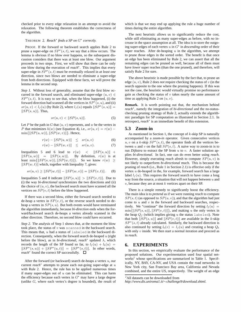
proposed solutions. Our experimentation used four spatial net-works2 whose specifications are summarized in Table 1. Specif-ically, NY, BAY, CA-NV, and USA contain the road networks inNew York city, San Francisco Bay area, California and Nevadacombined, and the entire US, respectively. The weight of an edge

2All datasets can be downloaded fromhttp://www.dis.uniroma1.it/∼challenge9/download.shtml.

dataset num. of vertices num. of edgesNY 264,346 733,846

BAY 321,270 800,172CA-NV 1,890,815 4,657,742

USA 23,947,347 58,333,344

Table 1: Dataset specifications

kdataset 4 6 8 10 12 14 16

NY 51% 38% 31% 26% 22% 20% 18%BAY 46% 33% 26% 22% 18% 16% 14%

CA-NV 46% 33% 21% 19% 16% 16% 15%USA 45% 32% 25% 21% 18% 16% 15%

(a) Vertex ratiodataset 4 6 8 10 12 14 16

NY 72% 65% 61% 58% 56% 53% 52%BAY 66% 57% 52% 48% 45% 43% 42%

CA-NV 63% 54% 49% 45% 43% 41% 40%USA 61% 51% 47% 44% 41% 39% 38%

(b) Edge ratio

Table 2: Sizes of k-skip graphs

equals the travel time on the corresponding road segment. All ofour results were obtained on a computer equipped with an IntelCore 2 DUO 3.0Ghz CPU and 2 Giga bytes memory, running Fe-dora Linux 13.

Size of the pre-computed structure. Our technique has the fea-ture of demanding only a structure with sub-linear size, i.e., a k-skip graph G = (V , E) occupies less space than the underlyingroad network G = (V,E). The first set of experiments demon-strates this by proving that G has fewer vertices and edges thanG. Equivalently, if we define the vertex ratio to be |V |/|V | andthe edge ratio to be |E|/|E|, the goal is to show that both ratiosare below 1 by a comfortable margin. Moreover, remember that V

is a k-skip cover (Definition 3). Hence, the vertex ratio also reflectsthe effectiveness of the AS algorithm in Section 4.2.

Table 2a presents the vertex ratios of each dataset as k variesfrom 4 to 16. Interestingly, we noticed that the ratio roughly equals2/k in all cases, that is, AS finds a k-skip cover with size about2|V |/k. In the same style, Table 2b shows the corresponding edgeratios, which are also much lower than 1, and decrease with theincrease of k. A general observation is that, both ratios tend to besmaller (i.e., greater size reduction) when the underlying networkis sparser (NY is the densest among all the datasets).

Query characteristics. Ideally, a k-skip SP query should be an-swered much faster than its traditional counterpart (that retrievesthe whole path). Next, we compare the reach algorithm devel-oped in Section 5.2 against reach, which is the state of the art forthe (traditional) SP problem, as reviewed in Section 2.1. We alsoexamined a method reach-on-supergraph that can be regarded as acompromise of the two algorithms. As mentioned in Section 5.2,any SP algorithm can be applied to produce a k-skip SP by findinga SP on the k-skip graph G. Following this rationale, reach-on-supergraph is a k-skip solution that simply employs reach on G.As a reference, we also report the performance of Dijkstra.

The cost of each method is measured as its average response timein processing a workload of 1000 queries whose source and desti-nation are both randomly selected from the vertices of the originalnetwork G. Figures 9a-9d plot the costs of alternative solutions asa function of k for the four datasets, respectively. The overhead of

reach reach-on-supergraph reach

0

0.2

0.4

0.6

0.8

1

1.2

1.4

1.6

4 6 8 10 12 14 16k

milli-seconds

0

0.2

0.4

0.6

0.8

1

1.2

1.4

1.6

4 6 8 10 12 14 16k

milli-seconds

(a) NY (Dijkstra = 15ms) (b) BAY (Dijkstra = 21ms)

0

1

2

3

4

5

6

7

8

9

4 6 8 10 12 14 16k

milli-seconds

0

10

20

30

40

50

60

70

4 6 8 10 12 14 16k

milli-seconds

(c) CA-NV (Dijkstra = 168ms) (d) USA (Dijkstra = 3300ms)

Figure 9: Cost of k-skip and traditional SP queries

Dijkstra is given separately beside the dataset name, because it issubstantially slower than all other competitors.

Both k-skip algorithms reach and reach-on-supergraph outper-form reach significantly. Furthermore, their performance gainsover reach become increasingly obvious as k grows larger (reachis irrelevant to k as it always reports the entire SP). This, therefore,validates k-skip graph as an effective methodology to attack thek-skip SP problem. Between the two k-skip algorithms, the con-sistent superiority of reach ascertains the necessity of designing anew algorithm that is able to leverage the characteristics of k-skipgraphs. Remember that reach gleans its performance advantagesat very little space overhead, because only one extra value needs tobe stored for each edge in G.

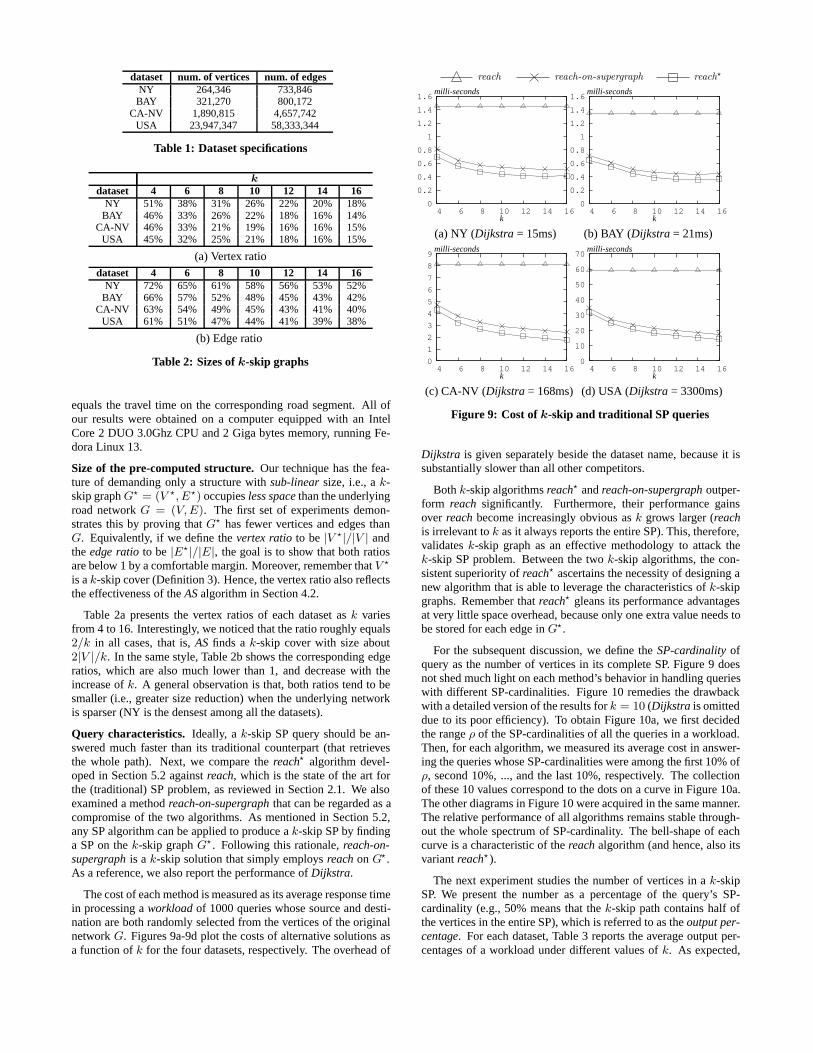
For the subsequent discussion, we define the SP-cardinality ofquery as the number of vertices in its complete SP. Figure 9 doesnot shed much light on each method’s behavior in handling querieswith different SP-cardinalities. Figure 10 remedies the drawbackwith a detailed version of the results for k = 10 (Dijkstra is omitteddue to its poor efficiency). To obtain Figure 10a, we first decidedthe range ρ of the SP-cardinalities of all the queries in a workload.Then, for each algorithm, we measured its average cost in answer-ing the queries whose SP-cardinalities were among the first 10% ofρ, second 10%, ..., and the last 10%, respectively. The collectionof these 10 values correspond to the dots on a curve in Figure 10a.The other diagrams in Figure 10 were acquired in the same manner.The relative performance of all algorithms remains stable through-out the whole spectrum of SP-cardinality. The bell-shape of eachcurve is a characteristic of the reach algorithm (and hence, also itsvariant reach).

The next experiment studies the number of vertices in a k-skipSP. We present the number as a percentage of the query’s SP-cardinality (e.g., 50% means that the k-skip path contains half ofthe vertices in the entire SP), which is referred to as the output per-centage. For each dataset, Table 3 reports the average output per-centages of a workload under different values of k. As expected,

reach reach-on-supergraph reach

0

0.2

0.4

0.6

0.8

1

1.2

1.4

1.6

1.8

0 200 400 600 800SP cardinality

milli-seconds

0 0

0.2 0.4 0.6 0.8

1 1.2 1.4 1.6 1.8

2 2.2

0 200 400 600 800 10001200SP cardinality

milli-seconds

0

(a) NY (b) BAY

0

2

4

6

8

10

12

14

1k 2k 3k 4kSP cardinality

milli-seconds

0 0

10

20

30

40

50

60

70

80

90

2k 4k 6k 8k 10k 12kSP cardinality

milli-seconds

0

(c) CA-NV (d) USA

Figure 10: Query cost vs. the number of vertices in the com-plete SP (k = 10)

kdataset 4 6 8 10 12 14 16

NY 55% 41% 34% 29% 27% 24% 22%BAY 52% 36% 29% 25% 22% 20% 18%

CA-NV 52% 36% 29% 25% 22% 21% 19%USA 51% 35% 28% 24% 22% 20% 19%

Table 3: Number of vertices in a k-skip SP (in percentage ofthe SP-cardinality)

the percentage decreases as k increases. It is not hard to observea strong correlation between the output percentages and the vertexratios in Table 2.

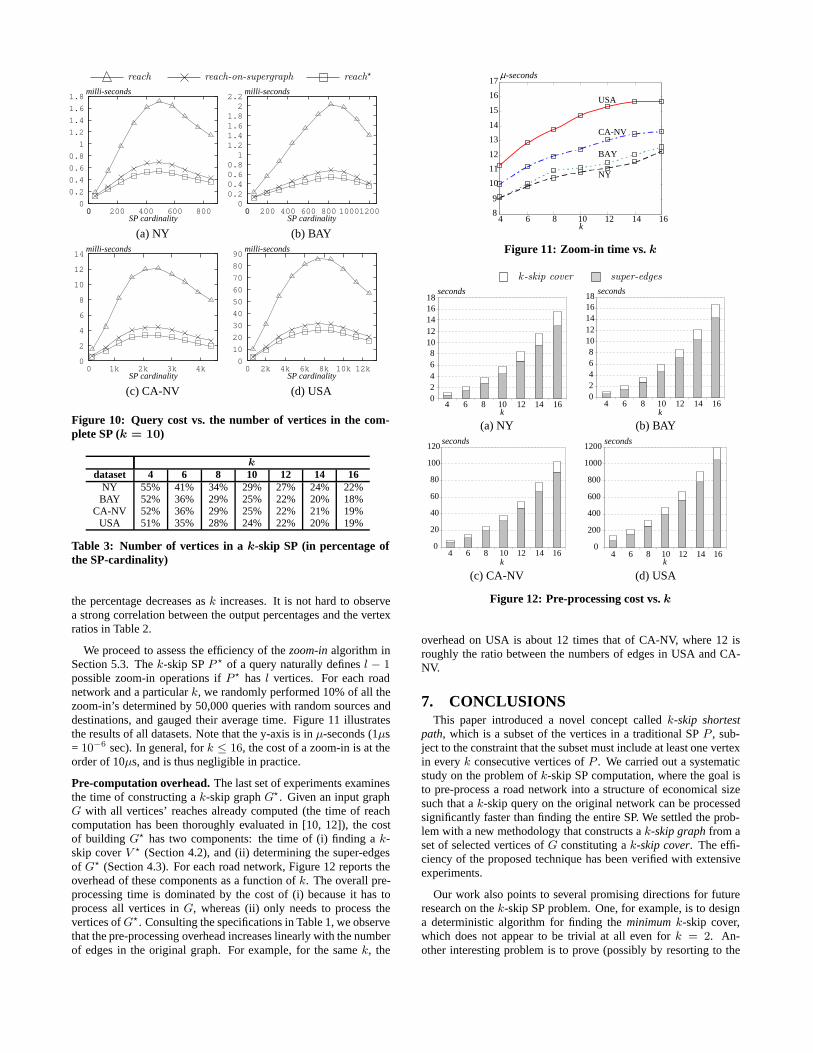
We proceed to assess the efficiency of the zoom-in algorithm inSection 5.3. The k-skip SP P of a query naturally defines l − 1possible zoom-in operations if P has l vertices. For each roadnetwork and a particular k, we randomly performed 10% of all thezoom-in’s determined by 50,000 queries with random sources anddestinations, and gauged their average time. Figure 11 illustratesthe results of all datasets. Note that the y-axis is in µ-seconds (1µs= 10−6 sec). In general, for k ≤ 16, the cost of a zoom-in is at theorder of 10µs, and is thus negligible in practice.

Pre-computation overhead. The last set of experiments examinesthe time of constructing a k-skip graph G. Given an input graphG with all vertices’ reaches already computed (the time of reachcomputation has been thoroughly evaluated in [10, 12]), the costof building G has two components: the time of (i) finding a k-skip cover V (Section 4.2), and (ii) determining the super-edgesof G (Section 4.3). For each road network, Figure 12 reports theoverhead of these components as a function of k. The overall pre-processing time is dominated by the cost of (i) because it has toprocess all vertices in G, whereas (ii) only needs to process thevertices of G. Consulting the specifications in Table 1, we observethat the pre-processing overhead increases linearly with the numberof edges in the original graph. For example, for the same k, the

8

9

10

11

12

13

14

15

16

17

4 6 8 10 12 14 16k

µ-seconds

USA

CA-NV

BAY

NY

Figure 11: Zoom-in time vs. k

k-skip cover super-edges

02468

1012141618

4 6 8 10 12 14 16k

seconds

k

seconds

02468

1012141618

4 6 8 10 12 14 16

(a) NY (b) BAY

k

seconds

0

20

40

60

80

100

120

4 6 8 10 12 14 16 k

seconds

0

200

400

600

800

1000

1200

4 6 8 10 12 14 16

(c) CA-NV (d) USA

Figure 12: Pre-processing cost vs. k

overhead on USA is about 12 times that of CA-NV, where 12 isroughly the ratio between the numbers of edges in USA and CA-NV.

7. CONCLUSIONSThis paper introduced a novel concept called k-skip shortest

path, which is a subset of the vertices in a traditional SP P , sub-ject to the constraint that the subset must include at least one vertexin every k consecutive vertices of P . We carried out a systematicstudy on the problem of k-skip SP computation, where the goal isto pre-process a road network into a structure of economical sizesuch that a k-skip query on the original network can be processedsignificantly faster than finding the entire SP. We settled the prob-lem with a new methodology that constructs a k-skip graph from aset of selected vertices of G constituting a k-skip cover. The effi-ciency of the proposed technique has been verified with extensiveexperiments.

Our work also points to several promising directions for futureresearch on the k-skip SP problem. One, for example, is to designa deterministic algorithm for finding the minimum k-skip cover,which does not appear to be trivial at all even for k = 2. An-other interesting problem is to prove (possibly by resorting to the

highway dimension [1]) a theoretical upper bound on the numberof super-edges in a k-skip graph, which will immediately lead to abound on the overall space consumption of our technique. Finally,it is certainly an important direction to explore the semantics of k-skip SP as well as the corresponding algorithms on other types ofgraphs, such as social networks.

AcknowledgementsYufei Tao and Cheng Sheng were supported by grants GRF4173/08, GRF 4169/09, and GRF 4166/10 from HKRGC. Jian Peiwas supported by NSERC Discovery grants, NSERC DiscoveryAccelerator Supplement grants, and NRAS Research Team Pro-gram. We thank the anonymous reviewers for their constructivesuggestions on improving the paper.

8. REFERENCES

[1] I. Abraham, A. Fiat, A. V. Goldberg, and R. F. F. Werneck.Highway dimension, shortest paths, and provably efficientalgorithms. In Proceedings of the Annual ACM-SIAMSymposium on Discrete Algorithms (SODA), pages 782–793,2010.

[2] R. Agrawal and H. V. Jagadish. Algorithms for searchingmassive graphs. IEEE Transactions on Knowledge and DataEngineering (TKDE), 6(2):225–238, 1994.

[3] T. H. Cormen, C. E. Leiserson, R. L. Rivest, and C. Stein.Introduction to Algorithms, Second Edition. The MIT Press,2001.

[4] K. Deng, X. Zhou, H. T. Shen, S. W. Sadiq, and X. Li.Instance optimal query processing in spatial networks. TheVLDB Journal, 18(3):675–693, 2009.

[5] E. W. Dijkstra. A note on two problems in connexion withgraphs. Numerische Mathematik, 1:269–271, 1959.

[6] R. Durstenfeld. Algorithm 235: Random permutation.Communications of the ACM (CACM), 7(7):420, 1964.

[7] G. N. Frederickson. Fast algorithms for shortest paths inplanar graphs, with applications. SIAM Journal ofComputing, 16(6):1004–1022, 1987.

[8] R. Geisberger, P. Sanders, D. Schultes, and D. Delling.Contraction hierarchies: Faster and simpler hierarchicalrouting in road networks. In Proceedings of Workshop onExperimental Algorithms (WEA), pages 319–333, 2008.

[9] A. V. Goldberg and C. Harrelson. Computing the shortestpath: A∗ search meets graph theory. In Proceedings of theAnnual ACM-SIAM Symposium on Discrete Algorithms(SODA), pages 156–165, 2005.

[10] A. V. Goldberg, H. Kaplan, and R. F. Werneck. Reach forA∗: Shortest path algorithms with preprocessing. InProceedings of Workshop on Algorithm Engineering andExperiments (ALENEX), pages 38–51, 2006.

[11] A. Gubichev, S. J. Bedathur, S. Seufert, and G. Weikum. Fastand accurate estimation of shortest paths in large graphs. InProceedings of Conference on Information and KnowledgeManagement (CIKM), pages 499–508, 2010.

[12] R. J. Gutman. Reach-based routing: A new approach toshortest path algorithms optimized for road networks. InProceedings of Workshop on Algorithm Engineering andExperiments (ALENEX), pages 100–111, 2004.

[13] P. E. Hart, N. J. Nilsson, and B. Raphael. A formal basis forthe heuristic determination of minimum cost paths. IEEETrans. Systems Science and Cybernetics, 4(2):100–107,1968.

[14] D. Haussler and E. Welzl. Epsilon-nets and simplex rangequeries. Discrete & Computational Geometry, 2:127–151,1987.

[15] D. A. Hutchinson, A. Maheshwari, and N. Zeh. An externalmemory data structure for shortest path queries. DiscreteApplied Mathematics, 126(1):55–82, 2003.

[16] N. Jing, Y.-W. Huang, and E. A. Rundensteiner. Hierarchicalencoded path views for path query processing: An optimalmodel and its performance evaluation. IEEE Transactions onKnowledge and Data Engineering (TKDE), 10(3):409–432,1998.

[17] S. Jung and S. Pramanik. An efficient path computationmodel for hierarchically structured topographical road maps.IEEE Transactions on Knowledge and Data Engineering(TKDE), 14(5):1029–1046, 2002.

[18] M. R. Kolahdouzan and C. Shahabi. Alternative solutions forcontinuous k nearest neighbor queries in spatial networkdatabases. GeoInformatica, 9(4):321–341, 2005.

[19] U. Lauther. An extremely fast, exact algorithm for findingshortest paths in static networks with geographicalbackground. Geoinformation und Mobilität - von derForschung zur praktischen Anwendung, 22:219–230, 2004.

[20] T. A. J. Nicholson. Finding the shortest route between twopoints in a network. The Computer Journal, 9:275–280,1966.

[21] M. Potamias, F. Bonchi, C. Castillo, and A. Gionis. Fastshortest path distance estimation in large networks. InProceedings of Conference on Information and KnowledgeManagement (CIKM), pages 867–876, 2009.

[22] M. N. Rice and V. J. Tsotras. Graph indexing of roadnetworks for shortest path queries with label restrictions.Proceedings of the VLDB Endowment (PVLDB), 4(2):69–80,2010.

[23] N. Robertson and P. D. Seymour. Graph minors. iii. planartree-width. Journal of Combinatorial Theory, Series B,36(1):49–64, 1984.

[24] H. Samet, J. Sankaranarayanan, and H. Alborzi. Scalablenetwork distance browsing in spatial databases. InProceedings of ACM Management of Data (SIGMOD), pages43–54, 2008.

[25] P. Sanders and D. Schultes. Highway hierarchies hastenexact shortest path queries. In Proceedings of EuropeanSymposium on Algorithms (ESA), pages 568–579, 2005.

[26] P. Sanders and D. Schultes. Engineering highwayhierarchies. In Proceedings of European Symposium onAlgorithms (ESA), pages 804–816, 2006.

[27] J. Sankaranarayanan, H. Samet, and H. Alborzi. Path oraclesfor spatial networks. Proceedings of the VLDB Endowment(PVLDB), 2(1):1210–1221, 2009.

[28] D. Wagner, T. Willhalm, and C. D. Zaroliagis. Geometriccontainers for efficient shortest-path computation. ACMJournal of Experimental Algorithmics, 10, 2005.

[29] F. Wei. Tedi: Efficient shortest path query answering ongraphs. In Proceedings of ACM Management of Data(SIGMOD), pages 99–110, 2010.

[30] Y. Xiao, W. Wu, J. Pei, W. Wang, and Z. He. Efficientlyindexing shortest paths by exploiting symmetry in graphs. InProceedings of Extending Database Technology (EDBT),pages 493–504, 2009.