Band Theory of Solids Semiconductor Theory Semiconductor Devices Nanotechnology
k · p THEORY OF SEMICONDUCTOR
NANOSTRUCTURESby
CALIN GALERIU, B.S., M.S., M.A.
A Dissertation
Submitted to the Faculty
of the
WORCESTER POLYTECHNIC INSTITUTE
in partial fulfillment of the requirements for the
Degree of Doctor of Philosophy
in
Physics
November 30, 2005
APPROVED:
Professor Lok C. Lew Yan Voon, Dissertation Advisor
Professor Richard S. Quimby, Committee Member
Professor Florin Catrina, Committee Member
Abstract
The objective of this project was to extend fundamentally the current k · p theory by applying
the Burt-Foreman formalism, rather than the conventional Luttinger-Kohn formalism, to a
number of novel nanostructure geometries. The theory itself was extended in two ways. First
in the application of the Burt-Foreman theory to computing the momentum matrix elements.
Second in the development of a new formulation of the multiband k · p Hamiltonian describing
cylindrical quantum dots.
A number of new and interesting results have been obtained. The computational imple-
mentation using the finite difference method of the Burt-Foreman theory for two dimensional
nanostructures has confirmed that a non-uniform grid is much more efficient, as had been ob-
tained by others in one dimensional nanostructures. In addition we have demonstrated that
the multiband problem can be very effectively and efficiently solved with commercial software
(FEMLAB).
Two of the most important physical results obtained and discussed in the dissertation are
the following. One is the first ab initio demonstration of possible electron localization in a
nanowire superlattice in a barrier material, using a full numerical solution to the one band k · pequation. The second is the demonstration of the exactness of the Sercel-Vahala transformation
for cylindrical wurtzite nanostructures. Comparison of the subsequent calculations to experi-
mental data on CdSe nanorods revealed the important role of the linear spin splitting term in
the wurtzite valence band.
ii
Acknowledgments
I would like to thank my advisor, Professor Lok C. Lew Yan Voon, for his patient guidance and
constant encouragement during the course of my research.
I would like to thank all members of our research group, and especially Professor Morten
Willatzen, Professor Roderik Melnik, Dr. Smagul Karazhanov, and Benny Lassen.
I would like to thank all faculty members, staff persons, and fellow students at Worcester
Polytechnic Institute.
I would like to thank my family, and especially my wife Luminita, for her patience and
support during my years of graduate studies.
I would like to thank my cat Pisoanca, who has kept me company during many hours of
typing and programming.
The research was supported through grants from the National Science Foundation, Grant
No. DMR-9984059 and Grant No. DMR-0454849, and by the Department of Physics at Worces-
ter Polytechnic Institute.
Copyright c©2005 by Calin Galeriu, all rights reserved.
iii
Contents
Abstract . . . . . . . . . . . . . . . . . . . . . . . . . . . . . . . . . . . . . . . . . ii
Acknowledgments . . . . . . . . . . . . . . . . . . . . . . . . . . . . . . . . . . . . iii
List of Figures . . . . . . . . . . . . . . . . . . . . . . . . . . . . . . . . . . . . . viii
List of Tables . . . . . . . . . . . . . . . . . . . . . . . . . . . . . . . . . . . . . . xi
1 Introduction 1
2 Symmetry and the calculation of matrix elements 5
2.1 Introduction . . . . . . . . . . . . . . . . . . . . . . . . . . . . . . . . . . . . . . . 5
2.2 Selection rules for matrix elements . . . . . . . . . . . . . . . . . . . . . . . . . . 5
2.3 Wigner-Eckart theorem . . . . . . . . . . . . . . . . . . . . . . . . . . . . . . . . 6
2.4 Momentum matrix elements at the Γ point in ZB structures . . . . . . . . . . . . 7
2.4.1 〈Γ15|Γ15|Γ1〉 momentum matrix elements . . . . . . . . . . . . . . . . . . . 8
2.4.2 〈Γ15|Γ15|Γ15〉 momentum matrix elements . . . . . . . . . . . . . . . . . . 8
2.4.3 〈Γ15|Γ15|Γ25〉 momentum matrix elements . . . . . . . . . . . . . . . . . . 8
2.4.4 〈Γ15|Γ15|Γ12〉 momentum matrix elements . . . . . . . . . . . . . . . . . . 8
2.5 Momentum matrix elements at the Γ point in DM structures . . . . . . . . . . . 9
2.6 Momentum matrix elements at the Γ point in WZ structures . . . . . . . . . . . 9
2.6.1 〈Γ1|Γ1|Γ1〉 momentum matrix elements . . . . . . . . . . . . . . . . . . . . 10
2.6.2 〈Γ1|Γ6|Γ6〉 momentum matrix elements . . . . . . . . . . . . . . . . . . . . 10
3 k · p theory - Kane 11
3.1 Introduction . . . . . . . . . . . . . . . . . . . . . . . . . . . . . . . . . . . . . . . 11
3.2 1-band model . . . . . . . . . . . . . . . . . . . . . . . . . . . . . . . . . . . . . . 11
3.3 2-band model, CB-VB coupling only . . . . . . . . . . . . . . . . . . . . . . . . . 13
3.3.1 Electron in GaAs . . . . . . . . . . . . . . . . . . . . . . . . . . . . . . . . 13
3.3.2 Light hole in GaAs . . . . . . . . . . . . . . . . . . . . . . . . . . . . . . . 13
3.4 4-band model, CB-VB coupling only . . . . . . . . . . . . . . . . . . . . . . . . . 13
3.5 3-band model . . . . . . . . . . . . . . . . . . . . . . . . . . . . . . . . . . . . . . 15
iv
3.5.1 k in the [1,0,0] direction . . . . . . . . . . . . . . . . . . . . . . . . . . . . 17
3.5.2 k in the [1,1,1] direction . . . . . . . . . . . . . . . . . . . . . . . . . . . . 18
3.6 6-band model . . . . . . . . . . . . . . . . . . . . . . . . . . . . . . . . . . . . . . 19
3.7 8-band model, CB-VB coupling only . . . . . . . . . . . . . . . . . . . . . . . . . 22
3.8 8-band model . . . . . . . . . . . . . . . . . . . . . . . . . . . . . . . . . . . . . . 25
3.9 Appendix A. Degenerate perturbation theory . . . . . . . . . . . . . . . . . . . . 29
3.10 Appendix B. Lowdin perturbation theory . . . . . . . . . . . . . . . . . . . . . . 31
4 k · p theory - Burt 33
4.1 Introduction . . . . . . . . . . . . . . . . . . . . . . . . . . . . . . . . . . . . . . . 33
4.2 Burt’s theory . . . . . . . . . . . . . . . . . . . . . . . . . . . . . . . . . . . . . . 34
4.3 Envelope function equations . . . . . . . . . . . . . . . . . . . . . . . . . . . . . . 35
4.4 Homogeneous semiconductor . . . . . . . . . . . . . . . . . . . . . . . . . . . . . 37
4.5 Burt’s Hamiltonian . . . . . . . . . . . . . . . . . . . . . . . . . . . . . . . . . . . 38
4.6 Burt’s Hamiltonian for ZB structures . . . . . . . . . . . . . . . . . . . . . . . . . 38
4.6.1 s = S, γ = Γ15, s′ = S . . . . . . . . . . . . . . . . . . . . . . . . . . . . . 39
4.6.2 s = S, γ = Γ15, s′ = X . . . . . . . . . . . . . . . . . . . . . . . . . . . . . 39
4.6.3 s = X, γ = Γ15, s′ = X . . . . . . . . . . . . . . . . . . . . . . . . . . . . . 40
4.6.4 s = X, γ = Γ25, s′ = X . . . . . . . . . . . . . . . . . . . . . . . . . . . . . 41
4.6.5 s = X, γ = Γ1, s′ = X . . . . . . . . . . . . . . . . . . . . . . . . . . . . . 41
4.6.6 s = X, γ = Γ12, s′ = X . . . . . . . . . . . . . . . . . . . . . . . . . . . . . 42
4.6.7 s = X, γ = Γ15, s′ = Y . . . . . . . . . . . . . . . . . . . . . . . . . . . . . 42
4.6.8 s = X, γ = Γ25, s′ = Y . . . . . . . . . . . . . . . . . . . . . . . . . . . . . 43
4.6.9 s = X, γ = Γ1, s′ = Y . . . . . . . . . . . . . . . . . . . . . . . . . . . . . 43
4.6.10 s = X, γ = Γ12, s′ = Y . . . . . . . . . . . . . . . . . . . . . . . . . . . . . 43
4.7 Conclusions . . . . . . . . . . . . . . . . . . . . . . . . . . . . . . . . . . . . . . . 44
4.7.1 Foreman’s notation . . . . . . . . . . . . . . . . . . . . . . . . . . . . . . . 45
4.8 Symmetrization versus Burt’s Hamiltonian . . . . . . . . . . . . . . . . . . . . . . 45
v
5 Momentum Matrix Elements 47
5.1 Introduction . . . . . . . . . . . . . . . . . . . . . . . . . . . . . . . . . . . . . . . 47
5.2 Calculation of 〈Ψ(N)(r)|pε|Ψ(M)(r)〉 . . . . . . . . . . . . . . . . . . . . . . . . . . 48
5.3 Calculation of 〈Ψ(N)(r)| ∂H∂kε
|Ψ(M)(r)〉 . . . . . . . . . . . . . . . . . . . . . . . . . 51
5.4 Normalization of the Wave Function . . . . . . . . . . . . . . . . . . . . . . . . . 51
5.5 The Effect of Symmetrization on the MME . . . . . . . . . . . . . . . . . . . . . 52
5.6 Appendix. The Projection Operator Method . . . . . . . . . . . . . . . . . . . . 54
6 k · p Theory under a Change of Basis 59
6.1 Introduction . . . . . . . . . . . . . . . . . . . . . . . . . . . . . . . . . . . . . . . 59
6.2 Mathematical Formalism . . . . . . . . . . . . . . . . . . . . . . . . . . . . . . . . 59
6.3 Diagonalization of the Spin-Orbit Interaction . . . . . . . . . . . . . . . . . . . . 60
6.3.1 ZB semiconductors . . . . . . . . . . . . . . . . . . . . . . . . . . . . . . . 61
6.3.2 WZ semiconductors . . . . . . . . . . . . . . . . . . . . . . . . . . . . . . 62
6.4 Rotation of the Cartesian Axes . . . . . . . . . . . . . . . . . . . . . . . . . . . . 62
6.4.1 Hamiltonian with no spin . . . . . . . . . . . . . . . . . . . . . . . . . . . 64
6.4.2 Hamiltonian with spin . . . . . . . . . . . . . . . . . . . . . . . . . . . . . 65
7 Strain in Cylindrical Heterostructures 67
7.1 Elasticity Theory in Cartesian Coordinates . . . . . . . . . . . . . . . . . . . . . 67
7.2 Elasticity Theory in Cylindrical Coordinates . . . . . . . . . . . . . . . . . . . . . 69
7.3 Plane Deformation with Cylindrical Symmetry . . . . . . . . . . . . . . . . . . . 70
7.4 Infinite Embedded Cylindrical Wire with Cubic Structure . . . . . . . . . . . . . 71
7.4.1 The Wire . . . . . . . . . . . . . . . . . . . . . . . . . . . . . . . . . . . . 73
7.4.2 The Substrate . . . . . . . . . . . . . . . . . . . . . . . . . . . . . . . . . 74
7.4.3 The Shrink Fit . . . . . . . . . . . . . . . . . . . . . . . . . . . . . . . . . 74
8 One-Band k · p Calculations - Quantum Ice Cream Dot 75
8.1 Introduction . . . . . . . . . . . . . . . . . . . . . . . . . . . . . . . . . . . . . . . 75
8.2 Effect of Dirichlet and van Neumann boundary conditions . . . . . . . . . . . . . 76
vi
9 One-Band k · p Calculations - Elliptical Dot 81
9.1 Introduction . . . . . . . . . . . . . . . . . . . . . . . . . . . . . . . . . . . . . . . 81
9.2 The Eigenstates of an Elliptical Quantum Dot . . . . . . . . . . . . . . . . . . . . 81
10 One-Band k · p Calculations - Nanowire Superlattice 85
10.1 Introduction . . . . . . . . . . . . . . . . . . . . . . . . . . . . . . . . . . . . . . . 85
10.2 Theory . . . . . . . . . . . . . . . . . . . . . . . . . . . . . . . . . . . . . . . . . . 86
10.3 Computational Models . . . . . . . . . . . . . . . . . . . . . . . . . . . . . . . . . 87
10.4 FDM applied to a unit cell with PBC . . . . . . . . . . . . . . . . . . . . . . . . 88
10.5 FDM applied to a finite number of unit cells . . . . . . . . . . . . . . . . . . . . . 92
10.6 Equivalent Kronig-Penney model . . . . . . . . . . . . . . . . . . . . . . . . . . . 93
10.7 Results and Discussions . . . . . . . . . . . . . . . . . . . . . . . . . . . . . . . . 94
10.7.1 Physical Applications: Inversion . . . . . . . . . . . . . . . . . . . . . . . 99
10.7.2 Physical Applications: Embedded nanowire . . . . . . . . . . . . . . . . . 100
10.8 Conclusions . . . . . . . . . . . . . . . . . . . . . . . . . . . . . . . . . . . . . . . 101
11 Eight-Band k · p Calculations - ZB Quantum Well 103
11.1 Introduction . . . . . . . . . . . . . . . . . . . . . . . . . . . . . . . . . . . . . . . 103
11.2 The Hamiltonian . . . . . . . . . . . . . . . . . . . . . . . . . . . . . . . . . . . . 104
11.3 The Finite Difference Method . . . . . . . . . . . . . . . . . . . . . . . . . . . . . 107
11.4 The Structure of Non-Zero Elements . . . . . . . . . . . . . . . . . . . . . . . . . 109
11.5 Generation of the Sparse Matrix . . . . . . . . . . . . . . . . . . . . . . . . . . . 110
11.6 Electronic Structure and MME for a Quantum Well . . . . . . . . . . . . . . . . 110
12 Six-Band k · p Calculations - WZ Cylindrical Dot 121
12.1 Introduction . . . . . . . . . . . . . . . . . . . . . . . . . . . . . . . . . . . . . . . 121
12.2 Hamiltonian . . . . . . . . . . . . . . . . . . . . . . . . . . . . . . . . . . . . . . . 122
12.3 Numerical Results and Discussion . . . . . . . . . . . . . . . . . . . . . . . . . . . 129
12.4 Conclusions . . . . . . . . . . . . . . . . . . . . . . . . . . . . . . . . . . . . . . . 132
13 Summary 133
vii
List of Figures
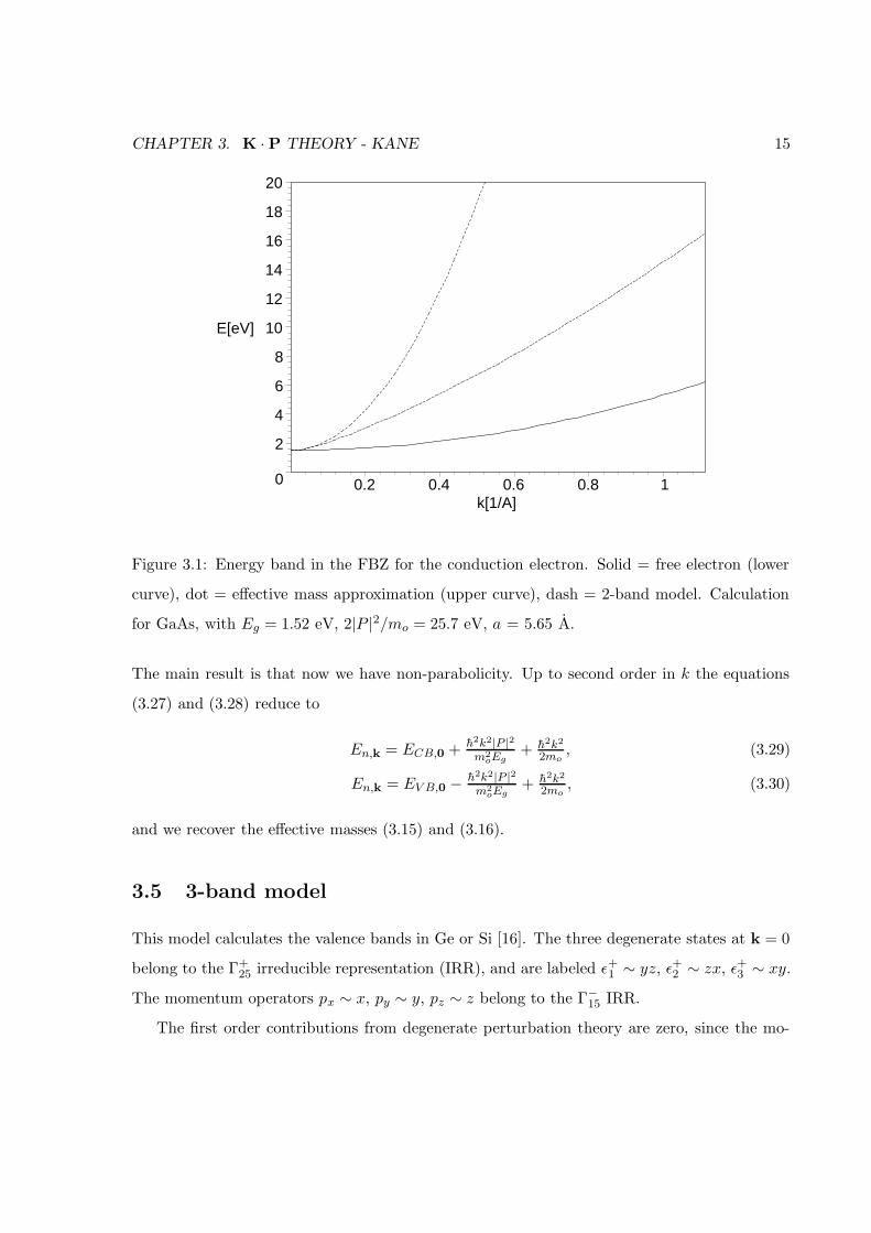
3.1 Energy band in the FBZ for the conduction electron. Solid = free electron (lower
curve), dot = effective mass approximation (upper curve), dash = 2-band model.
Calculation for GaAs, with Eg = 1.52 eV, 2|P |2/mo = 25.7 eV, a = 5.65 A. . . . 15
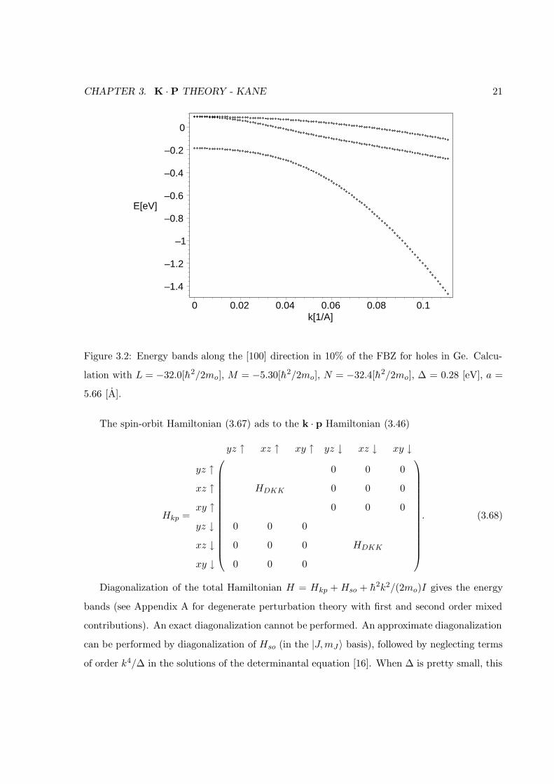
3.2 Energy bands along the [100] direction in 10% of the FBZ for holes in Ge.
Calculation with L = −32.0[h2/2mo], M = −5.30[h2/2mo], N = −32.4[h2/2mo],
∆ = 0.28 [eV], a = 5.66 [A]. . . . . . . . . . . . . . . . . . . . . . . . . . . . . . 21
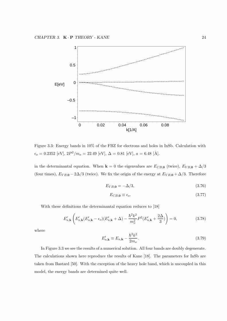
3.3 Energy bands in 10% of the FBZ for electrons and holes in InSb. Calculation
with εo = 0.2352 [eV], 2P 2/mo = 22.49 [eV], ∆ = 0.81 [eV], a = 6.48 [A]. . . . . 24
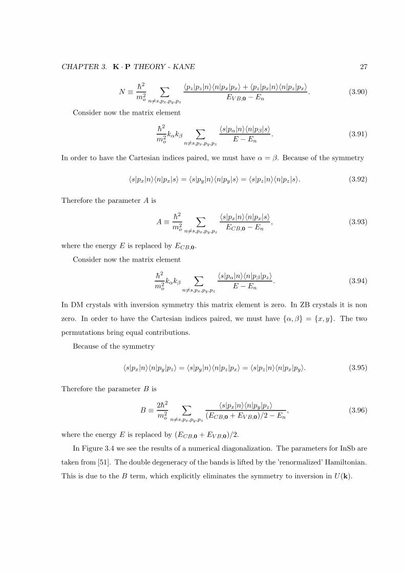
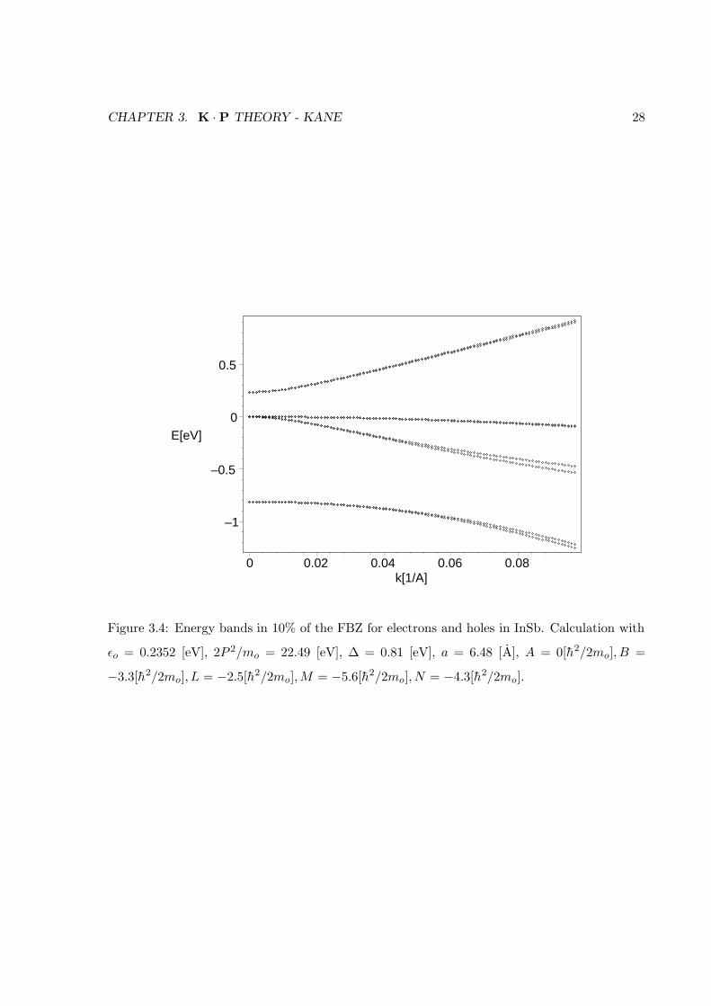
3.4 Energy bands in 10% of the FBZ for electrons and holes in InSb. Calculation
with εo = 0.2352 [eV], 2P 2/mo = 22.49 [eV], ∆ = 0.81 [eV], a = 6.48 [A],
A = 0[h2/2mo], B = −3.3[h2/2mo], L = −2.5[h2/2mo],M = −5.6[h2/2mo], N =
−4.3[h2/2mo]. . . . . . . . . . . . . . . . . . . . . . . . . . . . . . . . . . . . . . 28
6.1 The polar angles θ and φ. . . . . . . . . . . . . . . . . . . . . . . . . . . . . . . 61
7.1 The wire and the substrate before embedding. . . . . . . . . . . . . . . . . . . . 69
7.2 The wire and the substrate after the ”shrink fit” embedding. The shaded re-
gions are the compressed wire before insertion (right) and the relaxed wire after
insertion (left). . . . . . . . . . . . . . . . . . . . . . . . . . . . . . . . . . . . . . 69
8.1 The 10o QIC dot embedded into a cubical substrate. . . . . . . . . . . . . . . . 73
8.2 The 10o QIC wave-function in a YZ cross-section, at half X. . . . . . . . . . . . 74
8.3 The 10o QIC wave-function in a YZ cross-section, at half X. Contour plot lines
at 0.01, 0.02, etc. . . . . . . . . . . . . . . . . . . . . . . . . . . . . . . . . . . . 75
8.4 The 10o QIC wave-function along the Z axis. The three vertical domains are
the barrier, the quantum dot, and the barrier. . . . . . . . . . . . . . . . . . . . 76
9.1 Energy of the bound states for an elliptic quantum dot as a function of the
eccentricity a/b. The effective electron mass is m∗=0.041 mo, the product of the
two semi-axes is (ab)1/2 = 10 nm, the potential in the barrier is Vo = 0.7527 eV.
The strength of the well, deffined by γ =√
(2m∗/h2)abVo, is γ = 9. . . . . . . . 80
viii
10.1 A model nanowire superlattice. The parameters are: radius R, well width Lw,
barrier width Lb, effective mass in the well mw, effective mass in the barrier mb,
and the band offset V. . . . . . . . . . . . . . . . . . . . . . . . . . . . . . . . . . 83
10.2 The domain for (a) a unit cell with periodic boundary conditions and (b) a finite
number of unit cells, with barrier layers at both ends. . . . . . . . . . . . . . . . 84
10.3 Indexing of points on the non-uniform grid. • at grid points. × at midway points. 85
10.4 Detailed structure of the non-uniform grid at the well-barrier interface. Grid
steps of 1, 0.5, 0.25, 0.125, 0.0625, 0.03125, and 0.025 A are used. . . . . . . . . 90
10.5 Ground state for the NWSL calculated with the FEM (dotted black curve),
the FDM with uniform grid (solid gray curve), the FDM with non-uniform grid
(dotted gray curve), and the equivalent Kronig-Penney model (solid black curve). 91
10.6 Miniband formation in a symmetric NWSL structure. Energy levels as a function
of the number of wells. The segments on the right side are the energy bands
for the infinite NWSL, calculated with the FDM with non-uniform grid (left
segments) and with the equivalent Kronig-Penney model (right segments). L = 0,
L = 1, and L = 2, in increasing order of the energy. . . . . . . . . . . . . . . . . 92
10.7 Miniband formation in an asymmetric NWSL structure. Energy levels as a
function of the number of wells. The segments on the right side are the energy
bands for the infinite NWSL, calculated with the FDM with non-uniform grid
(left segment) and with the equivalent Kronig-Penney model (right segment).
L = 0. . . . . . . . . . . . . . . . . . . . . . . . . . . . . . . . . . . . . . . . . . 93
10.8 An energy band in the full Brillouin zone, calculated using the FDM with uni-
form grid (squares), the FDM with non-uniform grid (circles), and the equivalent
Kronig-Penney model (diamonds). The quantum numbers are L = 0, N = 1,
M = 1. . . . . . . . . . . . . . . . . . . . . . . . . . . . . . . . . . . . . . . . . . 93
10.9 Ground state for the NWSL calculated with the FDM with uniform grid (lower
dotted curve), the FDM with non-uniform grid (upper dotted curve), and the
equivalent Kronig-Penney model (solid curve). . . . . . . . . . . . . . . . . . . . 94
ix
10.10 Ground state for the NWSL calculated with the FDM with non-uniform grid
for a radius of 18 A (solid curve) compared to a radius of 100 A (dashed curve).
The left layer is AlGaAs, the right layer is GaAs. . . . . . . . . . . . . . . . . . 95
10.11 Lowest energy band in the first Brillouin zone for a finite outside barrier V
= 1.878 eV (squares, lower curve) compared to an infinite barrier one (circles,
upper curve). The structure is the same in both cases (radius of 100 A). . . . . 96
11.1 AlGaAs QW band structure. (eight-band calculation) . . . . . . . . . . . . . . 107
11.2 AlGaAs QW band structure. (six-band calculation) . . . . . . . . . . . . . . . . 108
11.3 AlAs QW band structure. (six-band calculation) . . . . . . . . . . . . . . . . . 109
11.4 AlGaAs momentum matrix elements: x polarization. (eight-band calculation) . 110
11.5 AlGaAs momentum matrix elements: x polarization. (six-band calculation) . . 111
11.6 AlAs momentum matrix elements: x polarization. (six-band calculation) . . . . 112
11.7 AlGaAs momentum matrix elements: z polarization. (eight-band calculation) . 113
11.8 AlGaAs momentum matrix elements: z polarization. (six-band calculation) . . 114
11.9 AlAs momentum matrix elements: z polarization. (six-band calculation) . . . . 115
12.1 The energies of the top three valence sublevels of a WZ GaN cylindrical quantum
dot, calculated with the 3D program (circles). The solid lines are the converged
values obtained with the 2D program. . . . . . . . . . . . . . . . . . . . . . . . . 124
12.2 The energies of the lowest states as a function of the CdSe quantum dot aspect
ratio. The linear term is not included in the Hamiltonian. Shown are the first
four states with Fz = 1/2 (solid lines) and with Fz = 3/2 (dotted lines). . . . . . 125
12.3 The energies of the lowest states as a function of the CdSe quantum dot aspect
ratio. The linear term is included in the Hamiltonian. Shown are the first four
states with Fz = 1/2 (solid lines) and with Fz = 3/2 (dotted lines). . . . . . . . 125
x
List of Tables
2.4 Some IRR, their dimensions, and their basis functions, for the symmetry group
Td. . . . . . . . . . . . . . . . . . . . . . . . . . . . . . . . . . . . . . . . . . . . 7
2.5 Some IRR, their dimensions, and their basis functions, for the symmetry group
O. . . . . . . . . . . . . . . . . . . . . . . . . . . . . . . . . . . . . . . . . . . . . 9
2.6 Some IRR, their dimensions, and their basis functions, for the symmetry group
C6v . . . . . . . . . . . . . . . . . . . . . . . . . . . . . . . . . . . . . . . . . . . . 10
11.2 Burt Hamiltonian, 4 bands and no spin. . . . . . . . . . . . . . . . . . . . . . . 99
11.6 8-band Kane parameters for GaAs, Al0.3Ga0.7As, and AlAs. . . . . . . . . . . . 106
11.6 6-band Kane parameters for GaAs, Al0.3Ga0.7As, and AlAs. . . . . . . . . . . . 107
12.3 6-band parameters for WZ GaN and CdSe. . . . . . . . . . . . . . . . . . . . . 126
xi
Chapter 1
Introduction
The invention of the solid state transistor in 1947 launched the age of semiconductor based
electronics. Over the last decade optical fiber communication has become the choice for the
world wide communication network. Semiconductor based light sources and detectors are crit-
ically important to this emerging technology. Progress in optoelectronics has occurred not so
much by device scaling as by new device physics. For example, the use of quantum wells in the
active region of lasers has reduced threshold current density by an order of magnitude [1].
A semiconductor heterostructure can have a quantum confinement in one dimension (quan-
tum well), two dimensions (quantum wire), or three dimensions (quantum dot) [2]. Laser
operation in a quantum wells was demonstrated in 1974. AlGaAs/GaAs was the first het-
erostructure ever made and enjoyed the most success in many areas. Today the InP based laser
dominates the optical fiber communications. In the past several years the nitride system [3] has
attracted a lot of attentions due to its wide bandgap, which gives blue light sources. Quantum
wires offer lateral confinement beyond the confinement in the growth direction, which will fur-
ther decrease the threshold current and increase the differential gain. Quantum dot structures
have discrete density of electronic states and in this regard they behave more like atoms rather
than solids.
The current state of research in this field is principally one of applying existing theories to
various nanostructures. The most commonly used method, in particular with optoelectronic
device modeling in mind, is based upon the conventional Luttinger-Kohn (LK) model [4]. While
1
CHAPTER 1. INTRODUCTION 2
a competing first principles approach was already developed in the 80’s and 90’s by Burt and
Foreman (BF) [5, 6, 7, 8, 9, 10, 11, 12], the application of the latter was until recently limited
to only demonstrating the differences between the two theories for quantum well structures.
Therefore the approach taken for this Ph.D. project was to generalize the application of the
BF theory to higher confinement nanostructures and to calculate physical properties beyond
just band structures, namely optical momentum matrix elements, since the later are relevant
to modeling optoelectronic devices. The other area of focus of this project is related to the
current interest in the influence of size and shape on physical properties [13]. Indeed in the
last few years there has been tremendous activity in the investigation, both theoretical and
experimental, of nanostructures with various shapes, such as nanorods, nanowires of different
cross-sectional shapes, and modulated nanowires. This has led us to apply the theory described
above to a number of different shapes. Details of the actual work now follow.
In Chapter 2 we discuss the role of symmetry in the calculation of matrix elements. The
k · p theory [14] relies heavily on the use of momentum matrix elements. Using symmetry
arguments [15] we can show that many of these matrix elements are zero, and many of them
are equal. This dramatically reduces the number of non-zero matrix elements that show up in
the k · p equations. The reduced number of these matrix elements also allows us to treat them
as fitting parameters, and to get their empirical values [16].
In Chapter 3 we discuss the k · p theory in the formulation of Kane [17, 18, 19, 20, 21, 22].
We give a detailed treatment of the 1-band, 4-band, 6-band, and 8-band Hamiltonians for bulk
ZB semiconductors. The derivation of the spin-orbit interaction and the folding-down of the
Hamiltonian [23] are treated in the greatest detail.
In Chapter 4 we discuss the k · p theory in the formulation of Burt [5, 6, 7, 8, 9, 10]. The
symmetry properties derived in Chapter 2 are now used extensively, and the 8-band Hamiltonian
for ZB heterostructures is obtained. Comparisons between calculations using the symmetrized
and the non-symmetrized Hamiltonians have been made for quantum wells [11, 24, 25, 26],
wires [27], and dots [28]. The differences between the Burt Hamiltonian and the symmetrized
one are pointed out.
In Chapter 5 we discuss the calculation of the momentum matrix elements. This is no easy
CHAPTER 1. INTRODUCTION 3
task, since the full eigenfunctions are never found, and only the eigenfunctions of the folded
down Hamiltonian are available [29, 30]. The formula for calculating the MME is derived in
the greatest detail, and the effects of using the Burt Hamiltonian or the symmetrized one are
shown.
In Chapter 6 we discuss the k · p theory under a change of basis. This happens when we
diagonalize the spin-orbit Hamiltonian [17, 31], but also when we rotate the Cartesian axes [18].
The theory developed in this chapter enables us to write very general and efficient computer
programs to deal with any possible crystallographic orientation of the heterostructure.
In Chapter 7 we discuss the calculation of strain in cylindrical heterostructures [32]. Al-
though we ignore strain in all calculations presented in this thesis, more detailed calculations
will have to include the effects of strain. The introduction of strain in a solid changes the lattice
parameters and the symmetry of the material. These in turn change the valence and conduction
bands [33].
In Chapter 8 we analyze a conical quantum dot, using a 1-band k · p method. The effect of
imposing Dirichlet or van Neumann boundary conditions is discussed.
In Chapter 9 we analyze an elliptical quantum dot, using a 1-band k · p method [34]. We
show that the eigenvalue equation is not separable, contrary to what was asserted in Ref. [35].
In Chapter 10 we analyze a nanowire superlattice (NWSL), using a 1-band k · p method
[36]. We derive the Hamiltonian in cylindrical coordinates, and we calculate the band structure.
Free-standing semiconductor NWSL have been grown experimentally [37, 38]. Extremely polar-
ized photoluminescence is one characteristic that makes NWSL likely candidates for practical
applications. In addition, a recent one-dimensional theory predicted the remarkable existence
of an inversion regime when the localization of the electron states can be reversed [39].
The calculation of intervalence subband optical transitions in quantum wells goes back to
a paper by Chang and James (CJ) in 1989 [40]. It established that these transitions can have
both TE and TM polarizations. The calculations were done using the four-band Luttinger-Kohn
(LK) Hamiltonian with infinite-barrier quantum-well states. Szmulowicz [29] generalized the CJ
equation to allow for position-dependent k ·p parameters. In Chapter 11 we present an envelope-
function-representation derivation and calculations of the band structure and the momentum
CHAPTER 1. INTRODUCTION 4
matrix elements between valence subbands in [001] quantum wells using the Luttinger-Kohn-
Kane and the Burt-Foreman Hamiltonians. We also discuss the numerical implementation of
the 8-band k · p method.
The III-V nitride semiconductors, with wurtzite (WZ) crystal structure, have received a
great deal of attention in recent years [41]. The detailed band structure of these materials was
studied after the discovery (in 1993) of blue light emission of WZ GaN on sapphire [3]. In
Chapter 12 we analyze a WZ cylindrical quantum dot, using a 6-band k · p method. We derive
the Hamiltonian in cylindrical coordinates, and we calculate the band structure, using a formu-
lation of the multiband envelope function theory first derived and applied by Sercel and Vahala
to spherical quantum dots and cylindrical quantum wires of zincblende (ZB) materials [42, 43].
We show that the formulation is exact for WZ materials, i.e., no axial approximation is needed.
The reduction in dimensionality greatly decreases the needed computational resources.
The above described work has resulted in five published papers:
1. L. C. Lew Yan Voon, C. Galeriu, M. Willatzen, Comment on: ”Confined states in two-
dimensional flat elliptic quantum dots and elliptic quantum wires”, Physica E 18 (2003),
547-549.
2. M. Willatzen, R. V. N. Melnik, C. Galeriu, L. C. Lew Yan Voon, Finite Element Analysis
of Nanowire Superlattice Structures, Proc. ICCSA 2003 (2003), 755-763.
3. C. Galeriu, L. C. Lew Yan Voon, R. Melnik, M. Willatzen, Modeling a nanowire superlat-
tice using the finite difference method in cylindrical polar coordinates, Computer Physics
Communications 157 (2004), 147-159.
4. M. Willatzen, R. V. N. Melnik, C. Galeriu, L. C. Lew Yan Voon, Quantum confinement
phenomena in nanowire superlattice structures, Mathematics and Computers in Simula-
tion 65 (2004), 385-397.
5. L. C. Lew Yan Voon, C. Galeriu, B. Lassen, M. Willatzen, R. Melnik, Electronic structure
of wurtzite quantum dots with cylindrical symmetry, Applied Physics Letters 87 (2005),
041906-1–041906-3.
Chapter 2
Symmetry and the calculation of
matrix elements
2.1 Introduction
An important component of the k · p theory is the application of group theory to reduce the
number of elements in the Hamiltonian. We provide our discussion of results derived in Ref. [15]
and Ref. [14].
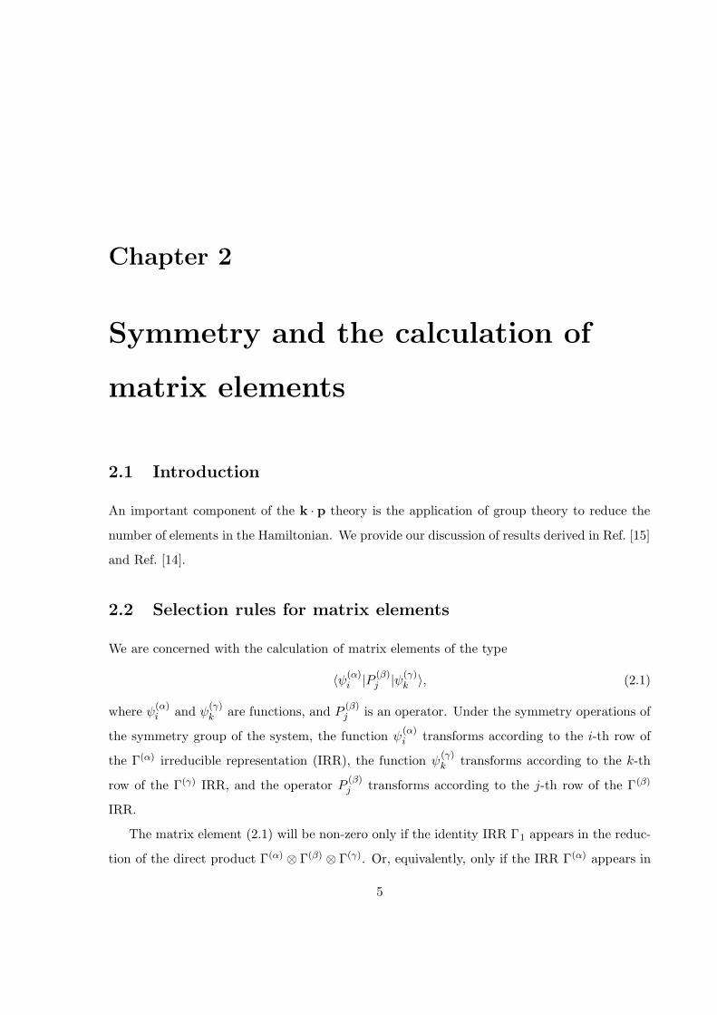
2.2 Selection rules for matrix elements
We are concerned with the calculation of matrix elements of the type
〈ψ(α)i |P (β)
j |ψ(γ)k 〉, (2.1)
where ψ(α)i and ψ
(γ)k are functions, and P
(β)j is an operator. Under the symmetry operations of
the symmetry group of the system, the function ψ(α)i transforms according to the i-th row of
the Γ(α) irreducible representation (IRR), the function ψ(γ)k transforms according to the k-th
row of the Γ(γ) IRR, and the operator P(β)j transforms according to the j-th row of the Γ(β)
IRR.
The matrix element (2.1) will be non-zero only if the identity IRR Γ1 appears in the reduc-
tion of the direct product Γ(α) ⊗ Γ(β) ⊗ Γ(γ). Or, equivalently, only if the IRR Γ(α) appears in
5
CHAPTER 2. SYMMETRY AND THE CALCULATION OF MATRIX ELEMENTS 6
the reduction of the direct product Γ(β) ⊗ Γ(γ), since the identity IRR Γ1 appears only in the
direct product of two identical IRR [44].
As a practical example we will analyze the momentum matrix elements at the k = 0 point
(Γ point) of a semiconductor with the zincblende (ZB) structure. The momentum operators
px = −ih∂/∂x, py = −ih∂/∂y, pz = −ih∂/∂z, and the valence-band functions |X〉, |Y 〉,|Z〉 transform according to the Γ15 IRR. The first conduction-band function |S〉 transforms
according to the Γ1 IRR.
Since [14]
Γ15 ⊗ Γ1 = Γ15, (2.2)
only functions F transforming according to Γ15 will produce non-zero matrix elements 〈F |pi|S〉.Since [14]
Γ15 ⊗ Γ15 = Γ1 ⊕ Γ12 ⊕ Γ15 ⊕ Γ25, (2.3)
only functions F transforming according to Γ1, Γ12, Γ15, or Γ25 will produce non-zero matrix
elements 〈F |pi|X〉,〈F |pi|Y 〉,〈F |pi|Z〉.
2.3 Wigner-Eckart theorem
The Wigner-Eckart theorem [45] states that
〈ψ(α)i |P (β)
j |ψ(γ)k 〉 = CG(i, j, k, α, β, γ)〈ψ(α) ||P (β)||ψ(γ)〉, (2.4)
where CG is a Clebsh-Gordan coefficient. This relation dramatically reduces the number of
independent matrix elements. Many of the matrix elements are eliminated because the Clebsh-
Gordan coefficient is zero.
However, since the Clebsh-Gordan coefficients are hard to find, we use an alternative method
to obtain the non-zero matrix elements. We use the fact that, under a symmetry operation G
of the symmetry group of the system, the functions and the operator transform according to
Gψ(α)i =
∑
u
ψ(α)u G
(α)ui , (2.5)
CHAPTER 2. SYMMETRY AND THE CALCULATION OF MATRIX ELEMENTS 7
where G(α)ui is a matrix element. Since point group operations leave inner products invariant,
the matrix element becomes [15]
〈ψ(α)i |P (β)
j |ψ(γ)k 〉 = 〈Gψ(α)
i |GP (β)j |Gψ(γ)
k 〉 =∑
u
∑
v
∑
w
G(α)ui G
(β)vj G
(γ)wk〈ψ(α)
u |P (β)v |ψ(γ)
w 〉. (2.6)
Although the triple sum (2.6) is intimidating, in practice, due to the G(α)ui G
(β)vj G
(γ)wk product,
only a few matrix elements remain in the sum. We are left with simple relations like
〈ψ(α)i |P (β)
j |ψ(γ)k 〉 = −〈ψ(α)
i |P (β)j |ψ(γ)
k 〉, (2.7)
which indicate that the respective matrix element is zero, or
〈ψ(α)i |P (β)
j |ψ(γ)k 〉 = 〈ψ(α)
u |P (β)v |ψ(γ)
w 〉, (2.8)
which indicate the equality of the two matrix elements. In rare occasions we obtain relations
between three or more matrix elements. In this case we have to solve the system of linear
equations in order to find the non-zero elements and the proportionality relations.
2.4 Momentum matrix elements at the Γ point in ZB structures
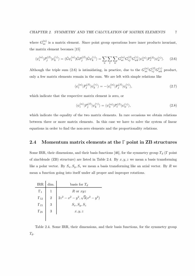
Some IRR, their dimensions, and their basis functions [46], for the symmetry group Td (Γ point
of zincblende (ZB) structure) are listed in Table 2.4. By x, y, z we mean a basis transforming
like a polar vector. By Sx, Sy, Sz we mean a basis transforming like an axial vector. By R we
mean a function going into itself under all proper and improper rotations.
IRR dim. basis for Td
Γ1 1 R or xyz
Γ12 2 2z2 − x2 − y2,√
3(x2 − y2)
Γ15 3 Sx, Sy, Sz
Γ25 3 x, y, z
Table 2.4. Some IRR, their dimensions, and their basis functions, for the symmetry group
Td.
CHAPTER 2. SYMMETRY AND THE CALCULATION OF MATRIX ELEMENTS 8
Knowing the basis functions, and knowing how x, y, z transform under the symmetry oper-
ations, allows us to find the matrices G(α) for the IRR α of interest and for all the 24 symmetry
operations G of the Td symmetry group. These matrices are listed in [47]. With these matri-
ces, the calculation of (2.6) is straightforward. For a given choice of i, j, k, α, γ (β = Γ15) the
calculation is performed for all 24 symmetry operations. The results are summarized below.
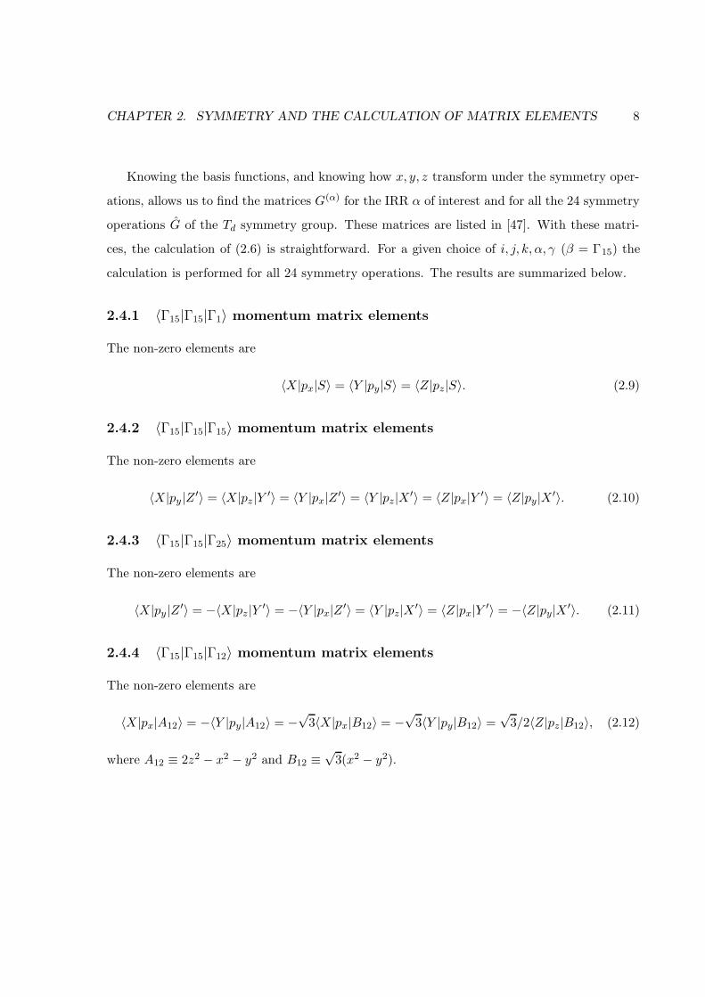
2.4.1 〈Γ15|Γ15|Γ1〉 momentum matrix elements
The non-zero elements are
〈X|px|S〉 = 〈Y |py|S〉 = 〈Z|pz|S〉. (2.9)
2.4.2 〈Γ15|Γ15|Γ15〉 momentum matrix elements
The non-zero elements are
〈X|py |Z ′〉 = 〈X|pz |Y ′〉 = 〈Y |px|Z ′〉 = 〈Y |pz|X ′〉 = 〈Z|px|Y ′〉 = 〈Z|py|X ′〉. (2.10)
2.4.3 〈Γ15|Γ15|Γ25〉 momentum matrix elements
The non-zero elements are
〈X|py |Z ′〉 = −〈X|pz |Y ′〉 = −〈Y |px|Z ′〉 = 〈Y |pz|X ′〉 = 〈Z|px|Y ′〉 = −〈Z|py|X ′〉. (2.11)
2.4.4 〈Γ15|Γ15|Γ12〉 momentum matrix elements
The non-zero elements are
〈X|px|A12〉 = −〈Y |py|A12〉 = −√
3〈X|px|B12〉 = −√
3〈Y |py|B12〉 =√
3/2〈Z|pz|B12〉, (2.12)
where A12 ≡ 2z2 − x2 − y2 and B12 ≡√
3(x2 − y2).
CHAPTER 2. SYMMETRY AND THE CALCULATION OF MATRIX ELEMENTS 9
2.5 Momentum matrix elements at the Γ point in DM struc-
tures
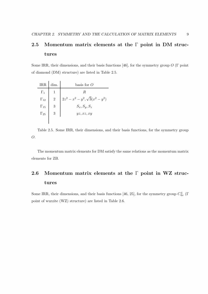
Some IRR, their dimensions, and their basis functions [46], for the symmetry group O (Γ point
of diamond (DM) structure) are listed in Table 2.5.
IRR dim. basis for O
Γ1 1 R
Γ12 2 2z2 − x2 − y2,√
3(x2 − y2)
Γ15 3 Sx, Sy, Sz
Γ25 3 yz, xz, xy
Table 2.5. Some IRR, their dimensions, and their basis functions, for the symmetry group
O.
The momentum matrix elements for DM satisfy the same relations as the momentum matrix
elements for ZB.
2.6 Momentum matrix elements at the Γ point in WZ struc-
tures
Some IRR, their dimensions, and their basis functions [46, 25], for the symmetry group C 46v (Γ
point of wurzite (WZ) structure) are listed in Table 2.6.
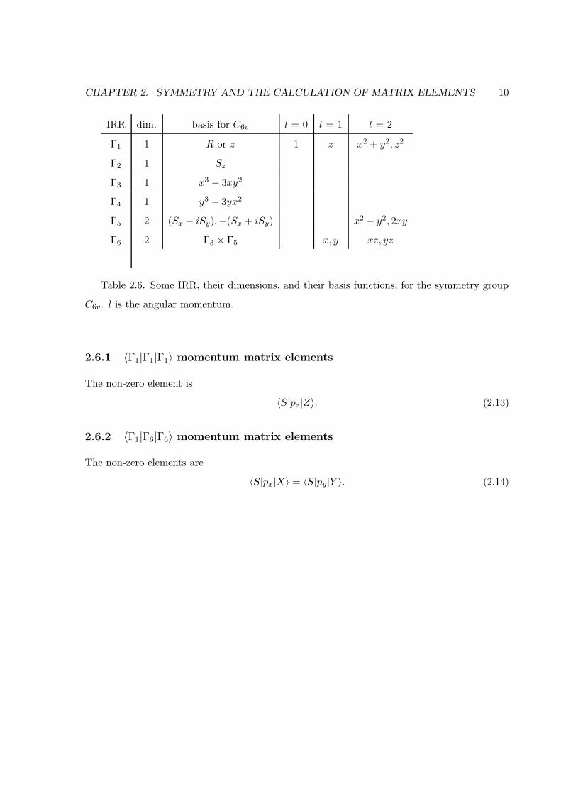
CHAPTER 2. SYMMETRY AND THE CALCULATION OF MATRIX ELEMENTS 10
IRR dim. basis for C6v l = 0 l = 1 l = 2
Γ1 1 R or z 1 z x2 + y2, z2
Γ2 1 Sz
Γ3 1 x3 − 3xy2
Γ4 1 y3 − 3yx2
Γ5 2 (Sx − iSy),−(Sx + iSy) x2 − y2, 2xy
Γ6 2 Γ3 × Γ5 x, y xz, yz
Table 2.6. Some IRR, their dimensions, and their basis functions, for the symmetry group
C6v. l is the angular momentum.
2.6.1 〈Γ1|Γ1|Γ1〉 momentum matrix elements
The non-zero element is
〈S|pz|Z〉. (2.13)
2.6.2 〈Γ1|Γ6|Γ6〉 momentum matrix elements
The non-zero elements are
〈S|px|X〉 = 〈S|py|Y 〉. (2.14)
Chapter 3
k · p theory - Kane
3.1 Introduction
In this chapter we present a review of the k · p method. The k · p method was originally an
application of the perturbation method to the study of energy bands and wave functions in
the vicinity of some important points in k space. The paper of Dresselhaus, Kip, and Kittel
[16] established the importance of the k · p approach as a rigorous basis for the empirical
determination of band structure. Symmetry arguments are used by the k · p method to show
that the band structure in a small region of k space depends only on a few parameters. Extensive
derivations and calculations using the k · p method, and many review papers by E.O. Kane
[17, 18, 19, 20, 21, 22] have transformed this perturbative approach into one of the main methods
used in Solid State Physics.
3.2 1-band model
The simplest example for an application of the k · p theory is when the electronic state is non-
degenerate and only weakly interacting with all other states. In this situation we have to solve
the one electron Schrodinger equation
Hψn,k(r) = En,kψn,k(r), (3.1)
11
CHAPTER 3. K · P THEORY - KANE 12
with the Hamiltonian
H =p2
2mo+ V (r) +
h
4m2oc
2(σ ×∇V ) · p, (3.2)
and the Bloch wave-function
ψn,k(r) = eik·run,k(r). (3.3)
Since
(−ih∇)eik·run,k(r) = hkeik·run,k(r) + eik·r(−ih∇)un,k(r), (3.4)
(−ih∇)2eik·run,k(r) = h2k2eik·run,k(r)+2hk · eik·r(−ih∇)un,k(r)+ eik·r(−ih∇)2un,k(r), (3.5)
substitution of (3.3) into (3.1) gives(h2k2
2mo+
2hk · p2mo
+p2
2mo+ V (r) +
h
4m2oc
2(σ ×∇V ) · (hk + p)
)un,k(r) = En,kun,k(r). (3.6)
With the notation
π = p +h
4moc2(σ ×∇V ), (3.7)
equation (3.6) becomes(H +
h2k2
2mo+
h
mok · π
)un,k(r) = En,kun,k(r). (3.8)
Equation (3.8) is solved using second order non-degenerate perturbation theory. The pertur-
bation is the k dependent part of the Hamiltonian. The solution, up to second order, is:
En,k = En,0 +h2k2
2mo+hk
mo· 〈n, 0|π|n, 0〉 +
h2
m2o
∑
m6=n
|k · 〈n, 0|π|m, 0〉|2En,0 −Em,0
. (3.9)
Since the energy band has a minimum at k = 0, the term linear in k is zero. We introduce the
Cartesian indices α, β = x, y, z, and assume Einstein’s summation convention for these indices.
We have
En,k = En,0 +h2k2
2mo+h2
m2o
kαkβ
∑
m6=n
〈n, 0|πα|m, 0〉〈m, 0|πβ |n, 0〉En,0 −Em,0
, (3.10)
En,k = En,0 +h2
2kαkβ
(1
m∗n
)
α,β
, (3.11)
where the tensor of the effective mass is
(1
m∗n
)
α,β
=
(1
mo
)δα,β +
2
m2o
∑
m6=n
〈n, 0|πα|m, 0〉〈m, 0|πβ |n, 0〉En,0 −Em,0
. (3.12)
CHAPTER 3. K · P THEORY - KANE 13
3.3 2-band model, CB-VB coupling only
In this model the spin is not considered. The conduction band consists of one non-degenerate
band |s〉 and the valence band consists of three degenerate bands |px〉, |py〉, |pz〉. The 2-band
model considers the coupling of the conduction band to one of the valence bands. Perturbation
theory is applied to the two bands independently.
3.3.1 Electron in GaAs
We consider coupling of the s band only with the three valence bands, which are closest in
energy. The calculation of matrix elements gives
〈s|pα|pβ〉 = Pδα,β , (3.13)
〈pγ |pα|pβ〉 = 0. (3.14)
Symmetry requires the three non-zero elements to be equal. Therefore the effective mass is
isotropic. Introducing the energy gap Eg ≡ ECB,0 −EV B,0 we get
1
m∗CB
=1
mo+
2|P |2m2
oEg. (3.15)
3.3.2 Light hole in GaAs
Along a given k direction, [kx, 0, 0] as an example, only one of the three valence bands will
couple to the conduction band. This is due to (3.13)-(3.14). Therefore we can treat that band
with non-degenerate perturbation theory. The effective mass is again isotropic, and usually
negative.1
m∗V B
=1
mo− 2|P |2m2
oEg. (3.16)
3.4 4-band model, CB-VB coupling only
This model allows coupling only between the one CB and the three VB, and ignores completely
the influences of the other bands. Spin is not considered. Within this approximation, the
CHAPTER 3. K · P THEORY - KANE 14
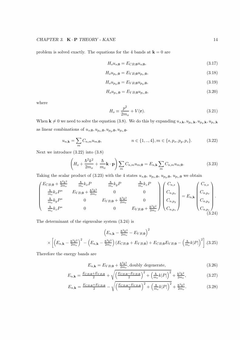
problem is solved exactly. The equations for the 4 bands at k = 0 are
Hous,0 = ECB,0us,0, (3.17)
Houpx,0 = EV B,0upx,0, (3.18)
Houpy,0 = EV B,0upy,0, (3.19)
Houpz ,0 = EV B,0upz ,0, (3.20)
where
Ho ≡ p2
2mo+ V (r). (3.21)
When k 6= 0 we need to solve the equation (3.8). We do this by expanding us,k, upx,k, upy ,k, upz,k
as linear combinations of us,0, upx,0, upy,0, upz ,0.
un,k =∑
m
Cn,mum,0, n ∈ 1, .., 4,m ∈ s, px, py, pz. (3.22)
Next we introduce (3.22) into (3.8)(Ho +
h2k2
2mo+
h
mok · p
)∑
m
Cn,mum,0 = En,k
∑
m
Cn,mum,0. (3.23)
Taking the scalar product of (3.23) with the 4 states us,0, upx,0, upy,0, upz ,0 we obtain
ECB,0 + h2k2
2mo
hmokxP
hmokyP
hmokzP
hmokxP
∗ EV B,0 + h2k2
2mo0 0
hmokyP
∗ 0 EV B,0 + h2k2
2mo0
hmokzP
∗ 0 0 EV B,0 + h2k2
2mo
Cn,s
Cn,px
Cn,py
Cn,pz
= En,k
Cn,s
Cn,px
Cn,py
Cn,pz
.
(3.24)
The determinant of the eigenvalue system (3.24) is
(En,k − h2k2
2mo−EV B,0
)2
×[(En,k − h2k2
2mo
)2−(En,k − h2k2
2mo
)(ECB,0 +EV B,0) +ECB,0EV B,0 −
(h
mok|P |
)2].(3.25)
Therefore the energy bands are
En,k = EV B,0 + h2k2
2mo,doubly degenerate, (3.26)
En,k =ECB,0+EV B,0
2 +
√(ECB,0−EV B,0
2
)2+(
hmok|P |
)2+ h2k2
2mo, (3.27)
En,k =ECB,0+EV B,0
2 −√(
ECB,0−EV B,0
2
)2+(
hmok|P |
)2+ h2k2
2mo. (3.28)
CHAPTER 3. K · P THEORY - KANE 15
0
2
4
6
8
10
12
14
16
18
20
E[eV]
0.2 0.4 0.6 0.8 1k[1/A]
Figure 3.1: Energy band in the FBZ for the conduction electron. Solid = free electron (lower
curve), dot = effective mass approximation (upper curve), dash = 2-band model. Calculation
for GaAs, with Eg = 1.52 eV, 2|P |2/mo = 25.7 eV, a = 5.65 A.
The main result is that now we have non-parabolicity. Up to second order in k the equations
(3.27) and (3.28) reduce to
En,k = ECB,0 + h2k2|P |2m2
oEg+ h2k2
2mo, (3.29)
En,k = EV B,0 − h2k2|P |2m2
oEg+ h2k2
2mo, (3.30)
and we recover the effective masses (3.15) and (3.16).
3.5 3-band model
This model calculates the valence bands in Ge or Si [16]. The three degenerate states at k = 0
belong to the Γ+25 irreducible representation (IRR), and are labeled ε+1 ∼ yz, ε+2 ∼ zx, ε+3 ∼ xy.
The momentum operators px ∼ x, py ∼ y, pz ∼ z belong to the Γ−15 IRR.
The first order contributions from degenerate perturbation theory are zero, since the mo-
CHAPTER 3. K · P THEORY - KANE 16
mentum operator is odd under inversion, while the ε+ functions are even.
〈ε+r |pα|ε+s 〉 = 0, r, s ∈ 1, 2, 3, α ∈ x, y, z. (3.31)
In other words
Γ+1 /∈ Γ+
25 ⊗ Γ−15 ⊗ Γ+
25. (3.32)
The second order contributions from degenerate perturbation theory are due to the matrix
elements
Hrs =h2
m2o
kαkβ
∑
n6=ε+
〈ε+r |pα|n〉〈n|pβ|ε+s 〉EV B,0 −En
. (3.33)
Because of the symmetry
〈xy|pz|n〉 = 〈yz|px|n〉 = 〈zx|py|n〉, (3.34)
〈xy|px|n〉 = 〈yz|py|n〉 = 〈zx|pz |n〉 = 〈xy|py|n〉 = 〈yz|pz|n〉 = 〈zx|px|n〉. (3.35)
Consider the case r = s. In the group of DM there are symmetry operators that invert only
one coordinate. The matrix element 〈ε+r |pα|n〉〈n|pβ|ε+r 〉 would cancel unless α = β. The matrix
elements, with the help of (3.35), can be written as
H11 = Lk2x +M(k2
y + k2z), (3.36)
H22 = Lk2y +M(k2
x + k2z), (3.37)
H33 = Lk2z +M(k2
x + k2y), (3.38)
where
L =h2
m2o
∑
n6=ε+
〈yz|px|n〉〈n|px|yz〉EV B,0 −En
, (3.39)
M =h2
m2o
∑
n6=ε+
〈yz|py|n〉〈n|py|yz〉EV B,0 −En
. (3.40)
Consider the case r 6= s. In the matrix element 〈ε+r |pα|n〉〈n|pβ|ε+s 〉 we need to have all Cartesian
coordinates paired. Since ε+r and ε+s share one Cartesian coordinate, the two remaining Carte-
sian coordinates determine α and β. There will be two contributions to the matrix element,
since α and β are not uniquely determined, but up to a permutation. Nonetheless, the product
CHAPTER 3. K · P THEORY - KANE 17
kαkβ will factor out. The matrix elements, with the help of (3.35), can be written as
H12 = H21 = Nkxky, (3.41)
H13 = H31 = Nkxkz, (3.42)
H23 = H32 = Nkykz, (3.43)
where
N =h2
m2o
∑
n6=ε+
〈xy|pz|n〉〈n|px|yz〉 + 〈xy|px|n〉〈n|pz|yz〉EV B,0 −En
. (3.44)
The energy bands are given by
En,k = EV B,0 +h2k2
2mo+ λ, (3.45)
where λ is an eigenvalue of the DKK Hamiltonian
HDKK =
Lk2x +M(k2
y + k2z) Nkxky Nkxkz
Nkxky Lk2y +M(k2
x + k2z) Nkykz
Nkxkz Nkykz Lk2z +M(k2
x + k2y)
. (3.46)
For k in a general direction there will be three different eigenvalues.
3.5.1 k in the [1,0,0] direction
When kx = k, ky = 0, kz = 0 the DKK Hamiltonian reduces to
HDKK =
Lk2 0 0
0 Mk2 0
0 0 Mk2
, (3.47)
with eigenvalues
λ1 = Lk2, (3.48)
λ2 = Mk2, (3.49)
λ3 = Mk2. (3.50)

CHAPTER 3. K · P THEORY - KANE 18
3.5.2 k in the [1,1,1] direction
When kx = k/√
3, ky = k/√
3, kz = k/√
3 the DKK Hamiltonian reduces to
HDKK =
(L+ 2M)k2/3 Nk2/3 Nk2/3
Nk2/3 (L+ 2M)k2/3 Nk2/3
Nk2/3 Nk2/3 (L+ 2M)k2/3
, (3.51)
with eigenvalues
λ1 = L+2M+2N3 k2, (3.52)
λ2 = L+2M−N3 k2, (3.53)
λ3 = L+2M−N3 k2. (3.54)
The point here is that we have introduced anisotropy. Only when L = M +N the effective
masses in the [1,0,0] and [1,1,1] directions are equal. If this is the case, the DKK Hamiltonian
becomes
HDKK =
Nk2x +Mk2 Nkxky Nkxkz
Nkxky Nk2y +Mk2 Nkykz
Nkxkz Nkykz Nk2z +Mk2
, (3.55)
with eigenvalues
λ1 = (M +N)k2, (3.56)
λ2 = Mk2, (3.57)
λ3 = Mk2. (3.58)
Therefore the effective mass is isotropic when L = M +N .
Another limiting case is when we restrict the interaction to only the first conduction band,
of symmetry s ∼ xyz. In this case
L = N = h2
m2o
〈yz|px|xyz〉〈xyz|px|yz〉EV B,0−ECB,0
= − h2|P |2m2
oEg, (3.59)
M = 0, (3.60)
and we recover the energy bands (3.26) and (3.30).
CHAPTER 3. K · P THEORY - KANE 19
3.6 6-band model
This is a generalization of the 3-band model, when we introduce the spin-orbit interaction.
The spin-orbit interactions is most easily treated as a perturbation acting on the cell periodic
function un,k. From eq. (3.6), this perturbation is
Hso =h
4m2oc
2(σ ×∇V ) · (hk + p). (3.61)
Since the velocity of the electron in its atomic orbit is very much greater than the velocity of
a wave packet made up of wave vectors in the neighborhood of k, the first term of Hso can be
neglected, leading to [17]:
Hso ≈ h
4m2oc
2(σ ×∇V ) · p =
h
4m2oc
2(∇V × p) · σ. (3.62)
∇V × p is an axial vector, which simplifies the matrix elements. We need to calculate the
matrix elements of the first order degenerate perturbation for the spin-orbit interaction. The
basis consists of ε+1 ↑∼ yz, ε+2 ↑∼ zx, ε+3 ↑∼ xy, ε+1 ↓∼ yz, ε+2 ↓∼ zx, ε+3 ↓∼ xy. Consider the
matrix element
〈ε+r |εαβγ∂V
∂xβpγ |ε+s 〉, r, s ∈ 1, 2, 3, α, β, γ ∈ x, y, z. (3.63)
When r = s the two Cartesian components γ and β are not paired, and the matrix element is
zero. When r 6= s, ε+r and ε+s share one Cartesian coordinate, and the two remaining Cartesian
coordinates determine β and γ, up to a permutation. The permutation, however, is already
included in the cross-product. Because of the symmetry, the non-zero elements will be equal:
〈yz|∂V∂x
py −∂V
∂ypx|xz〉 = 〈zx|∂V
∂ypz −
∂V
∂zpy|yx〉 = 〈xy|∂V
∂zpx − ∂V
∂xpz|zy〉 ≡ ∆
4m2oc
2
3ih. (3.64)
The transposed elements will have opposite sign, since the matrix elements are purely imaginary
(due to p = ih∇), and complex conjugation reduces to a change of sign. Therefore evaluation
CHAPTER 3. K · P THEORY - KANE 20
of the spatial part of the matrix elements of Hso gives
yz xz xy yz xz xy
yz 0 σz −σy 0 σz −σy
xz −σz 0 σx −σz 0 σx
xy σy −σx 0 σy −σx 0
yz 0 σz −σy 0 σz −σy
xz −σz 0 σx −σz 0 σx
xy σy −σx 0 σy −σx 0
∆
3i. (3.65)
Now the evaluation of the spin part of the matrix elements of Hso is trivial, since the Pauli
matrices are [48]
σx =
↑ ↓
↑ 0 1
↓ 1 0
, σy =
↑ ↓
↑ 0 −i↓ i 0
, σz =
↑ ↓
↑ 1 0
↓ 0 −1
. (3.66)
Therefore the matrix elements of Hso are given by [17]
Hso =
yz ↑ xz ↑ xy ↑ yz ↓ xz ↓ xy ↓
yz ↑ 0 1 0 0 0 i
xz ↑ −1 0 0 0 0 1
xy ↑ 0 0 0 −i −1 0
yz ↓ 0 0 −i 0 −1 0
xz ↓ 0 0 1 1 0 0
xy ↓ i −1 0 0 0 0
∆
3i. (3.67)
CHAPTER 3. K · P THEORY - KANE 21
–1.4
–1.2
–1
–0.8
–0.6
–0.4
–0.2
0
E[eV]
0 0.02 0.04 0.06 0.08 0.1k[1/A]
Figure 3.2: Energy bands along the [100] direction in 10% of the FBZ for holes in Ge. Calcu-
lation with L = −32.0[h2/2mo], M = −5.30[h2/2mo], N = −32.4[h2/2mo], ∆ = 0.28 [eV], a =
5.66 [A].
The spin-orbit Hamiltonian (3.67) ads to the k · p Hamiltonian (3.46)
Hkp =
yz ↑ xz ↑ xy ↑ yz ↓ xz ↓ xy ↓
yz ↑ 0 0 0
xz ↑ HDKK 0 0 0
xy ↑ 0 0 0
yz ↓ 0 0 0
xz ↓ 0 0 0 HDKK
xy ↓ 0 0 0
. (3.68)
Diagonalization of the total Hamiltonian H = Hkp + Hso + h2k2/(2mo)I gives the energy
bands (see Appendix A for degenerate perturbation theory with first and second order mixed
contributions). An exact diagonalization cannot be performed. An approximate diagonalization
can be performed by diagonalization of Hso (in the |J,mJ 〉 basis), followed by neglecting terms
of order k4/∆ in the solutions of the determinantal equation [16]. When ∆ is pretty small, this
CHAPTER 3. K · P THEORY - KANE 22
approach is not justified (but it is necessary if you need to fit the experimental effective mass
in order to get the L,M,N parameters).
In Figure 3.2 we see the results of a numerical diagonalization. All three bands are doubly
degenerate, as expected from Kramer’s theorem. The calculations shown here reproduce the
results of Kane [17].
3.7 8-band model, CB-VB coupling only
This model applies to semiconductors with a direct gap, where both the CB and VB have a
minimum at k = 0. The 8-band model is an extension of the 4-band model, where we introduce
the spin-orbit coupling. The effect of the other bands is not considered. The spin-orbit coupling
is introduced as a perturbation, together with the k · p term. This is done to minimize the
number of parameters in the theory [20]. The spin-orbit coupling, if introduced in the k = 0
basis, will lift some of the degeneracy of the valence band states [49]. Therefore more parameters
will be introduced when we add the k · p interaction, due to the reduction in symmetry.
We use the same eigenfunctions from (3.17)-(3.20). A special phase convention will be
used, with the us,0 function purely imaginary. This is to make the matrix element P ≡i〈xyz|pz |xy〉 real. We expand un,k, (n=1..8), as linear combinations of us,0↑, upx,0↑, upy ,0↑, upz ,0↑,
us,0↓, upx,0↓, upy,0↓, upz ,0↓.
un,k =∑
m
Cn,m↑um,0↑ +∑
m
Cn,m↓um,0↓, n ∈ 1, .., 8,m ∈ s, px, py, pz. (3.69)
We write (3.6) as(Ho +
h2k2
2mo+hk · pmo
+h
4m2oc
2(σ ×∇V ) · (hk + p)
)un,k(r) = En,kun,k(r), (3.70)
where
Ho =p2
2mo+ V (r), (3.71)
is the unperturbed Hamiltonian (3.21). Next we introduce (3.69) into (3.70). Again, we neglect
the spin-orbit term linear in k.
(Ho + h2k2
2mo+ h
mok · p + h
4m2oc2
(σ ×∇V ) · p)
(∑
m Cn,m↑um,0↑ +∑
m Cn,m↓um,0↓)
= En,k (∑
m Cn,m↑um,0↑ +∑
m Cn,m↓um,0↓) . (3.72)
CHAPTER 3. K · P THEORY - KANE 23
Taking the scalar product of (3.72) with the 8 states us,0↑, upx,0↑, upy,0↑, upz,0↑, us,0↓, upx,0↓,
upy,0↓, upz ,0↓ we obtain
HCB−V B
Cn,s↑
Cn,px↑
Cn,py↑
Cn,pz↑
Cn,s↓
Cn,px↓
Cn,py↓
Cn,pz↓
= En,k
Cn,s↑
Cn,px↑
Cn,py↑
Cn,pz↑
Cn,s↓
Cn,px↓
Cn,py↓
Cn,pz↓
, (3.73)
where the Hamiltonian matrix has two parts
HCB−V B =
(H4 0
0 H4
)+
0 0 0 0 0 0 0 0
0 0 1 0 0 0 0 i
0 −1 0 0 0 0 0 1
0 0 0 0 0 −i −1 0
0 0 0 0 0 0 0 0
0 0 0 −i 0 0 −1 0
0 0 0 1 0 1 0 0
0 i −1 0 0 0 0 0
∆
3i. (3.74)
H4 is the matrix (3.24) calculated for the 4-band model, due to the k · p perturbation
H4 =
ECB,0 + h2k2
2mo
hmokxP
hmokyP
hmokzP
hmokxP EV B,0 + h2k2
2mo0 0
hmokyP 0 EV B,0 + h2k2
2mo0
hmokzP 0 0 EV B,0 + h2k2
2mo
. (3.75)
The spin-orbit part has been calculated in (3.67). Two more rows and columns (first and fifth)
are added for the conduction band. All these added matrix elements are zero, due to symmetry
(s ∼ xyz).
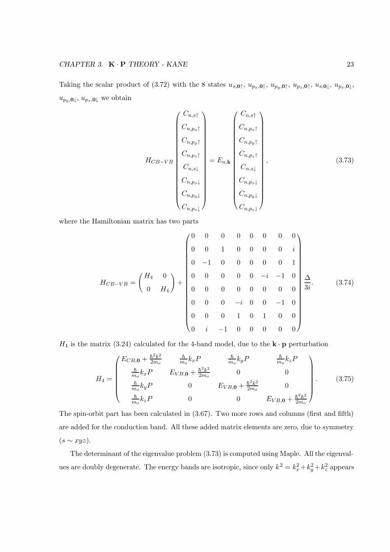
The determinant of the eigenvalue problem (3.73) is computed using Maple. All the eigenval-
ues are doubly degenerate. The energy bands are isotropic, since only k2 = k2x +k2
y +k2z appears
CHAPTER 3. K · P THEORY - KANE 24
–1
–0.5
0
0.5
1
E[eV]
0 0.02 0.04 0.06 0.08k[1/A]
Figure 3.3: Energy bands in 10% of the FBZ for electrons and holes in InSb. Calculation with
εo = 0.2352 [eV], 2P 2/mo = 22.49 [eV], ∆ = 0.81 [eV], a = 6.48 [A].
in the determinantal equation. When k = 0 the eigenvalues are ECB,0 (twice), EV B,0 + ∆/3
(four times), EV B,0 − 2∆/3 (twice). We fix the origin of the energy at EV B,0 +∆/3. Therefore
EV B,0 = −∆/3, (3.76)
ECB,0 ≡ εo. (3.77)
With these definitions the determinantal equation reduces to [18]
E′n,k
(E′
n,k(E′n,k − εo)(E
′n,k + ∆) − h2k2
m2o
P 2(E′n,k +
2∆
3)
)= 0, (3.78)
where
E′n,k ≡ En,k − h2k2
2mo. (3.79)
In Figure 3.3 we see the results of a numerical solution. All four bands are doubly degenerate.
The calculations shown here reproduce the results of Kane [18]. The parameters for InSb are
taken from Bastard [50]. With the exception of the heavy hole band, which is uncoupled in this
model, the energy bands are determined quite well.
CHAPTER 3. K · P THEORY - KANE 25
3.8 8-band model
This model is an extension of the previous model, when we include contributions from the other
energy bands. We include the other bands with the help of Lowdin perturbation theory [23]
(see Appendix B).
The basis function which we will use are un,0↑ and un,0↓, the eigenfunctions of the Hamilto-
nian (3.71), with spin added. The functions with n ∈ s, px, py, pz belong to the A class. The
full Hamiltonian
H =p2
2mo+ V (r) +
h2k2
2mo+hk · pmo
+h
4m2oc
2(σ ×∇V ) · (hk + p), (3.80)
will generate the matrix elements
Hmn ≡ 〈um,0|H|un,0〉. (3.81)
Lowdin perturbation theory requires us to solve self-consistently the system
∑
n∈A
Umncn = Ecm, m ∈ A, (3.82)
where the ’renormalized’ matrix elements are
Umn ≡ Hmn +∑
β∈B
HmβHβn
E −Hββ+ ... . (3.83)
Several approximations will now be used:
• The k dependent part of the spin-orbit interaction is ignored.
• The ’renormalized’ part of the spin-orbit interaction is ignored.
• The series of the ’renormalized’ matrix elements (3.83) is cut after the first order correction.
• The energy E in (3.83) is replaced with the approximate value (Hnn +Hmm)/2 [21].
CHAPTER 3. K · P THEORY - KANE 26
With these approximations the ’renormalized’ Hamiltonian becomes
U =
(H4 0
0 H4
)+
0 0 0 0 0 0 0 0
0 0 1 0 0 0 0 i
0 −1 0 0 0 0 0 1
0 0 0 0 0 −i −1 0
0 0 0 0 0 0 0 0
0 0 0 −i 0 0 −1 0
0 0 0 1 0 1 0 0
0 i −1 0 0 0 0 0
∆
3i+
(HR 0
0 HR
), (3.84)
where H4 is the direct k · p interaction
H4 =
ECB,0 + h2k2
2moi hmokxP i h
mokyP i h
mokzP
−i hmokxP EV B,0 + h2k2
2mo0 0
−i hmokyP 0 EV B,0 + h2k2
2mo0
−i hmokzP 0 0 EV B,0 + h2k2
2mo
, (3.85)
and HR is the ’renormalized’ part of the k · p interaction [22]
HR =
Ak2 Bkykz Bkxkz Bkxky
Bkykz Lk2x +M(k2
y + k2z) Nkxky Nkxkz
Bkxkz Nkxky Lk2y +M(k2
x + k2z) Nkykz
Bkxky Nkxkz Nkykz Lk2z +M(k2
x + k2y)
. (3.86)
The definition of the parameter P is
P ≡ −i〈s|px|px〉. (3.87)
The parameters L,M,N are closely related to those in the DKK Hamiltonian. The only differ-
ence is that now the sum does not include the first CB, which is now taken into account exactly,
and not within the perturbation. In these parameters the energy E from (3.83) is replaced by
EV B,0.
L ≡ h2
m2o
∑
n6=s,px,py,pz
〈px|px|n〉〈n|px|px〉EV B,0 −En
, (3.88)
M ≡ h2
m2o
∑
n6=s,px,py,pz
〈px|py|n〉〈n|py|px〉EV B,0 −En
, (3.89)
CHAPTER 3. K · P THEORY - KANE 27
N ≡ h2
m2o
∑
n6=s,px,py,pz
〈pz|pz|n〉〈n|px|px〉 + 〈pz|px|n〉〈n|pz|px〉EV B,0 −En
. (3.90)
Consider now the matrix element
h2
m2o
kαkβ
∑
n6=s,px,py,pz
〈s|pα|n〉〈n|pβ|s〉E −En
. (3.91)
In order to have the Cartesian indices paired, we must have α = β. Because of the symmetry
〈s|px|n〉〈n|px|s〉 = 〈s|py|n〉〈n|py|s〉 = 〈s|pz|n〉〈n|pz|s〉. (3.92)
Therefore the parameter A is
A ≡ h2
m2o
∑
n6=s,px,py,pz
〈s|px|n〉〈n|px|s〉ECB,0 −En
, (3.93)
where the energy E is replaced by ECB,0.
Consider now the matrix element
h2
m2o
kαkβ
∑
n6=s,px,py,pz
〈s|pα|n〉〈n|pβ|pz〉E −En
. (3.94)
In DM crystals with inversion symmetry this matrix element is zero. In ZB crystals it is non
zero. In order to have the Cartesian indices paired, we must have α, β = x, y. The two
permutations bring equal contributions.
Because of the symmetry
〈s|px|n〉〈n|py|pz〉 = 〈s|py|n〉〈n|pz|px〉 = 〈s|pz|n〉〈n|px|py〉. (3.95)
Therefore the parameter B is
B ≡ 2h2
m2o
∑
n6=s,px,py,pz
〈s|px|n〉〈n|py|pz〉(ECB,0 +EV B,0)/2 −En
, (3.96)
where the energy E is replaced by (ECB,0 +EV B,0)/2.
In Figure 3.4 we see the results of a numerical diagonalization. The parameters for InSb are
taken from [51]. The double degeneracy of the bands is lifted by the ’renormalized’ Hamiltonian.
This is due to the B term, which explicitly eliminates the symmetry to inversion in U(k).
CHAPTER 3. K · P THEORY - KANE 28
–1
–0.5
0
0.5
E[eV]
0 0.02 0.04 0.06 0.08k[1/A]
Figure 3.4: Energy bands in 10% of the FBZ for electrons and holes in InSb. Calculation with
εo = 0.2352 [eV], 2P 2/mo = 22.49 [eV], ∆ = 0.81 [eV], a = 6.48 [A], A = 0[h2/2mo], B =
−3.3[h2/2mo], L = −2.5[h2/2mo],M = −5.6[h2/2mo], N = −4.3[h2/2mo].
CHAPTER 3. K · P THEORY - KANE 29
3.9 Appendix A. Degenerate perturbation theory
Consider an unperturbed system with degenerate eigenstates. Sometimes the perturbation
Hamiltonian consists of two parts: one which contributes in first order, H (1), and one which
contributes in second order, H (2). If these two contributions have the same order of magnitude,
then it is better to write the perturbation expansion as [17]
H(λ) = H(0) + λ2H(1) + λH(2). (3.97)
In this way the first order contribution of H (1) will automatically be paired to the second order
contribution of H (2).We write the wave-function as
|ψ〉 = |ψ(0)〉 + λ|ψ(1)〉 + λ2|ψ(2)〉 + ... , (3.98)
and the energy as
E(λ) = E(0) + λE(1) + λ2E(2) + ... . (3.99)
We equate terms with same power in λ in Schrodinger’s equation
(H(0) + λ2H(1) + λH(2))(|ψ(0)〉 + λ|ψ(1)〉 + λ2|ψ(2)〉 + ...) =
(E(0) + λE(1) + λ2E(2) + ...)(|ψ(0)〉 + λ|ψ(1)〉 + λ2|ψ(2)〉 + ...). (3.100)
It follows that
H(0)|ψ(0)〉 = E(0)|ψ(0)〉, (3.101)
H(0)|ψ(1)〉 +H(2)|ψ(0)〉 = E(0)|ψ(1)〉 +E(1)|ψ(0)〉, (3.102)
H(0)|ψ(2)〉 +H(2)|ψ(1)〉 +H(1)|ψ(0)〉 = E(0)|ψ(2)〉 +E(1)|ψ(1)〉 +E(2)|ψ(0)〉. (3.103)
Consider the non-perturbed eigenvalue problem for the degenerate level n,m, ..., and for the
other levels α, β, ....
H(0)|ψn〉 = En|ψn〉, (3.104)
H(0)|ψα〉 = Eα|ψα〉. (3.105)
CHAPTER 3. K · P THEORY - KANE 30
The wave-function components will be written as
|ψ(0)〉 =∑
n c(0)n |ψn〉, (3.106)
|ψ(1)〉 =∑
n c(1)n |ψn〉 +
∑α c
(1)α |ψα〉. (3.107)
In writing (3.106) we have used (3.101) and (3.104). In the limit λ → 0 we recover the non-
perturbed states. Also
E(0) = En. (3.108)
We multiply (3.102) with 〈ψ(0)|. Using (3.101) and the fact that 〈ψ(0)|H(2)|ψ(0)〉 = 0, we obtain
E(1) = 0. (3.109)
We multiply (3.102) with 〈ψβ |, and using (3.105) we obtain
Eβc(1)β + 〈ψβ|H(2)|ψ(0)〉 = Enc
(1)β . (3.110)
Therefore the coefficient c(1)β is
c(1)β =
〈ψβ |H(2)|ψ(0)〉En −Eβ
. (3.111)
We multiply (3.103) with 〈ψm|, and using (3.104) we obtain
〈ψm|H(2)|ψ(1)〉 + 〈ψm|H(1)|ψ(0)〉 = E(2)c(0)m . (3.112)
Using (3.107) and the fact that 〈ψm|H(2)|ψn〉 = 0, the first term of (3.82) reduces to
〈ψm|H(2)|ψ(1)〉 = 〈ψm|H(2)|∑
α
c(1)α |ψα〉. (3.113)
Equation (3.112), with the help of (3.113) and (3.111), reduces to
∑
α
〈ψα|H(2)|ψ(0)〉En −Eα
〈ψm|H(2)|ψα〉 + 〈ψm|H(1)|ψ(0)〉 = E(2)c(0)m . (3.114)
By substitution of (3.106) we finally obtain
∑
n
(∑
α
〈ψm|H(2)|ψα〉〈ψα|H(2)|ψn〉En −Eα
+ 〈ψm|H(1)|ψn〉)c(0)n = E(2)c(0)m . (3.115)
Therefore the coefficients c(0)n and the energy E(2) are obtained by solving the eigenvalue problem
(3.115). In the particular case when H (1) = 0 we recover the simpler case of degenerate
perturbation theory with second order contributions [52].
CHAPTER 3. K · P THEORY - KANE 31
3.10 Appendix B. Lowdin perturbation theory
Consider a Hamiltonian H and a finite set of orthonormalized functions ψ(0)n , which are approx-
imate eigenfunctions of H. Suppose the set of functions ψ(0)n is split into to parts, A and B. We
will expand the eigenfunctions of H as
ψ =∑
n
cnψ(0)n . (3.116)
We substitute (3.116) into the eigenvalue equation
Hψ = Eψ. (3.117)
We take the scalar product of (3.117) with ψ(0)m and we obtain
∑nHmncn = Ecm, (3.118)
∑n6=mHmncn = (E −Hmm)cm, (3.119)
where
Hmn ≡ 〈ψ(0)m |H|ψ(0)
n 〉. (3.120)
From (3.119) we formally extract cm as
cm =∑
α∈A,α6=m
Hmα
E −Hmmcα +
∑
β∈B,β 6=m
Hmβ
E −Hmmcβ. (3.121)
From (3.121) we obtain cβ as
cβ =∑
α∈A
Hβα
E −Hββcα +
∑
γ∈B,γ 6=β
Hβγ
E −Hββcγ . (3.122)
We substitute (3.122) back into (3.121), and we iterate the process, with the ultimate goal of
eliminating all the cδ’s with δ ∈ B.
cm =∑
α∈A,α6=m
Hmα
E −Hmmcα +
∑
β∈B,β 6=m
Hmβ
E −Hmm
∑
α∈A
Hβα
E −Hββcα + ... . (3.123)
We choose m ∈ A and we write (3.123) as
∑
α∈A
Umαcα = Ecm, (m ∈ A), (3.124)
CHAPTER 3. K · P THEORY - KANE 32
with
Umα ≡ Hmα +∑
β∈B,β 6=m
HmβHβα
E −Hββ+ ..., (α ∈ A). (3.125)
We have therefore reduced the eigenvalue problem (3.118) on the full A + B space to the
restricted eigenvalue problem (3.124) on the A space. The effect of the B space is taken into
account through the ’renormalized’ matrix elements (3.125). Equations (3.124) and (3.125) are
solved iteratively, until convergence is achieved.
We choose m ∈ B and we write (3.123) as
cm =∑
α∈A
Umα
E −Hmmcα, (m ∈ B). (3.126)
In this way we have completely determined the coefficients of the eigenfunction expansion
(3.116).
Chapter 4
k · p theory - Burt
4.1 Introduction
The Kane model, developed in the previous chapter, deals with bulk semiconductors. The
periodicity characteristic to an infinite lattice has allowed us to apply the Bloch theorem. This
periodicity makes k a good quantum number.
However, when dealing with heterostructures, we no longer have periodicity. The question
has arisen, how can we still use Kane’s model when dealing with semiconductor quantum wells,
wires, and dots? Two empirical changes are applied to Kane’s Hamiltonian to extend its range
of applicability to heterostructures.
First, recognizing that the kx, ky, kz components have appeared by differentiation of the
exponential in the Bloch function
∇eik·r = ikeik·r, (4.1)
we replace these components by
kx → kx = −i ∂∂x, (4.2)
ky → ky = −i ∂∂y, (4.3)
kz → kz = −i ∂∂z. (4.4)
However, since the Kane parameters in the Hamiltonian now depend on position, being dif-
ferent in different semiconductors, they no longer commute with the differential operators. We
33
CHAPTER 4. K · P THEORY - BURT 34
therefore need an ordering of the Kane parameters and of the differentials in the Hamiltonian.
A popular choice is to symmetrize each individual element of the 8 × 8 Hamiltonian matrix.
This choice also guarantees that the resulting Hamiltonian is hermitian. The required changes
to Kane’s Hamiltonian are [53, 54]
Tkx → 1
2(T kx + kxT ), ... , (4.5)
Tkxky → 1
2(kxT ky + kyT kx), ... , (4.6)
where T represents any Kane parameter.
Symmetrized Hamiltonians have been successfully applied to the calculation of energy bands
in quantum wells [53, 54, 55], wires [56], and dots[57].
4.2 Burt’s theory
The arbitrariness of the symmetrization procedure has led Burt to believe that this is not
the right theory. Following a different approach, Burt chooses to derive the Hamiltonian for
a semiconductor heterostructure. He succeeded doing it in a series of papers [5, 6, 7, 8, 9],
culminating with a review article [10].
In Burt’s theory we start with a complete set of functions Un(r) that are periodic in the
position variable r. We assume that the different semiconductors of the heterojunction have
the same lattice constant, and the same Γ point Bloch functions. In fact, these zone-centre
eigenfunctions will be the ones used as Un(r). The wave-function is uniquely expanded as
Ψ(r) =∑
n
Fn(r)Un(r), (4.7)
where the envelope functions Fn(r) have a plane-wave expansion restricted to the first Brillouin
zone (FBZ).
Substitution of (4.7) into Schrodinger’s equation, and equating the coefficients of Un(r),
leads to the exact equation
−h2
2m∇2Fn(r) +
∑
n′
−ihm
pnn′ · ∇Fn′(r) +∑
n′
∫
UCHnn′(r, r′)Fn′(r′)dr′ = EFn(r), (4.8)
CHAPTER 4. K · P THEORY - BURT 35
where
pnn′ = 1Vc
∫UC U
∗n(r)pUn′(r)dr, (4.9)
Hnn′(r, r′) = Tnn′∆(r − r′) + Vnn′(r, r′), (4.10)
Tnn′ = 1Vc
∫UC U
∗n(r) p2
2mUn′(r)dr, (4.11)
∆(r − r′) = 1Ω
∑k∈FBZ e
ik·(r−r′), (4.12)
V (r)Ψ(r) =∑
n (∑
n′
∫UC Vnn′(r, r′)Fn′(r′)dr′)Un(r). (4.13)
The volume of a unit cell (UC) in real space is Vc, and in reciprocal space is Ω. The normalization
of the functions Un(r) is1
Vc
∫
UCU∗
n(r)Un′(r)dr = δnn′ . (4.14)
We further neglect non-local contributions in Hnn′(r, r′), and contributions from the inter-
face regions. We finally obtain the envelope function equation:
−h2
2m∇2Fn(r) +
∑
n′
−ihm
pnn′ · ∇Fn′(r) +∑
n′
Hnn′(r)Fn′(r) = EFn(r). (4.15)
Here Hnn′(r) is constant within a given homogeneous semiconductor region, equal to the bulk
value
Hnn′ =1
Vc
∫
UCU∗
n(r)H(r)Un′(r)dr, (4.16)
where H(r) is the Hamiltonian of the bulk semiconductor.
4.3 Envelope function equations
We divide the envelope functions into two categories: dominant ones, labeled with an index s,
and small ones, labeled with an index r.
We write the equation (4.15) for n = r
−h2
2m∇2Fr(r) +
∑
n′
−ihm
prn′ · ∇Fn′(r) +∑
n′
Hrn′(r)Fn′(r) = EFr(r). (4.17)
We now expand the sums as∑
n′
→∑
s′
+∑
r′
. (4.18)
CHAPTER 4. K · P THEORY - BURT 36
We neglect in (4.17) the first term (the small envelope function is slowly varying), and in the
sums over n′ we keep only the dominant terms (with s′) and the term containing Fr(r)
∑
s′
−ihm
prs′ · ∇Fs′(r) +∑
s′
Hrs′(r)Fs′(r) +Hrr(r)Fr(r) = EFr(r). (4.19)
In the end the envelope function Fr(r) is extracted as
Fr(r) =1
E −Hrr(r)
∑
s′
(−ihm
prs′ · ∇Fs′(r) +Hrs′(r)Fs′(r)
). (4.20)
We write the equation (4.15) for n = s
−h2
2m∇2Fs(r) +
∑
n′
−ihm
psn′ · ∇Fn′(r) +∑
n′
Hsn′(r)Fn′(r) = EFs(r). (4.21)
We now expand the sums as∑
n′
→∑
s”
+∑
r
. (4.22)
The expanded equation is
−h2
2m∇2Fs(r) +
∑
s”
−ihm
pss” · ∇Fs”(r) +∑
s”
Hss”(r)Fs”(r)
+∑
r
−ihm
psr · ∇Fr(r) +∑
r
Hsr(r)Fr(r) = EFs(r). (4.23)
We substitute Fr(r) from (4.20) into (4.23)
−h2
2m∇2Fs(r) +
∑
s”
−ihm
pss” · ∇Fs”(r) +∑
s”
Hss”(r)Fs”(r)
+∑
r
−ihm
psr · ∇[
1
E −Hrr(r)
∑
s′
(−ihm
prs′ · ∇Fs′(r) +Hrs′(r)Fs′(r)
)]
+∑
r
Hsr(r)1
E −Hrr(r)
∑
s′
(−ihm
prs′ · ∇Fs′(r) +Hrs′(r)Fs′(r)
)= EFs(r), (4.24)
−h2
2m∇2Fs(r) +
∑
s”
−ihm
pss” · ∇Fs”(r) +∑
s”
Hss”(r)Fs”(r)
+∑
r
∑
s′
−h2
m2psr · ∇
(prs′ · ∇Fs′(r)
E −Hrr(r)
)
+∑
r
∑
s′
−ihm
psr · ∇(
Hrs′(r)
E −Hrr(r)
)Fs′(r)
CHAPTER 4. K · P THEORY - BURT 37
+∑
r
∑
s′
−ihm
Hrs′(r)
E −Hrr(r)psr · ∇Fs′(r)
+∑
r
∑
s′
−ihm
Hsr(r)
E −Hrr(r)prs′ · ∇Fs′(r)
+∑
r
∑
s′
Hsr(r)Hrs′(r)
E −Hrr(r)Fs′(r) = EFs(r). (4.25)
We now neglect the terms from the 3-rd, 4-th, and 5-th lines in (4.25). The term on the 3-rd line
is non-zero only at an interface. The other two terms are also significant only at an interface,
being very small in the bulk of the semiconductors. We write the equation as
−h2
2m∇2Fs(r) +
∑
s”
−ihm
pss” · ∇Fs”(r) +∑
s”
Hss”(r)Fs”(r)
+∑
r
∑
s′
∑
α=x,y,z
∑
β=x,y,z
−h2
m2∂α
psrαprs′β
E −Hrr(r)∂βFs′(r)
+∑
r
∑
s′
Hsr(r)Hrs′(r)
E −Hrr(r)Fs′(r) = EFs(r). (4.26)
In (4.26) we have moved the momentum matrix element to the right of the differential, since it
doesn’t depend on position.
4.4 Homogeneous semiconductor
In the simpler case of a homogeneous semiconductor [7] the functions Un(r) are the zone-centre
eigenfunctions. We have only diagonal elements Hss, and the equation (4.26) becomes
−h2
2m∇2Fs(r) +
∑
s”
−ihm
pss” · ∇Fs”(r) +HssFs(r)
+∑
r
∑
s′
∑
α=x,y,z
∑
β=x,y,z
−h2
m2∂αpsrαprs′β
E −Hrr∂βFs′(r) = EFs(r). (4.27)
Because (4.27) is a differential equation with constant coefficients we can find solutions of
the form
Fs(r) = As(k)eik·r. (4.28)
The eigenvalue problem (4.27) becomes
h2k2
2mAs(k) +
∑
s”
h
mpss” · kAs”(k) +HssAs(k)
CHAPTER 4. K · P THEORY - BURT 38
+∑
r
∑
s′
∑
α=x,y,z
∑
β=x,y,z
h2
m2kαpsrαprs′β
E −HrrkβAs′(k) = EAs(k), (4.29)
which is the well known equation of the Kane model.
4.5 Burt’s Hamiltonian
We now apply the most dubious approximation of the Burt model, that the zone centre eigen-
functions are the same in all semiconductors of the quantum microstructure. This will again
generate only diagonal elements Hss(r), and the equation (4.26) becomes
−h2
2m∇2Fs(r) +
∑
s”
−ihm
pss” · ∇Fs”(r) +Hss(r)Fs(r)
+∑
r
∑
s′
∑
α=x,y,z
∑
β=x,y,z
−h2
m2∂α
psrαprs′β
E −Hrr(r)∂βFs′(r) = EFs(r). (4.30)
4.6 Burt’s Hamiltonian for ZB structures
We will investigate in great detail the Hamiltonian matrix element H(int)ss′ due to the interaction
of the dominant envelope functions with the remote ones.
H(int)ss′ =
∑
r
∑
α=x,y,z
∑
β=x,y,z
h2
m2kα
psrαprs′β
E −Hrr(r)kβ. (4.31)
We introduce Dirac’s notation for the momentum matrix elements. We label the remote bands
by their IRR γ, by an index nγ to distinguish between bands with the same IRR, and by an
index mγ to distinguish between basis functions of the same IRR.
H(int)ss′ =
∑
γ
∑
nγ
∑
mγ
∑
α=x,y,z
∑
β=x,y,z
h2
m2kα
〈s|pα|γ, nγ ,mγ〉〈γ, nγ ,mγ |pβ |s′〉E −Hγnγ (r)
kβ. (4.32)
We will now concentrate our attention on
∑
mγ
〈s|pα|γ, nγ ,mγ〉〈γ, nγ ,mγ |pβ|s′〉, (4.33)
for a given band (γ, nγ).
It is useful to notice that, if s or s′ belongs to Γ1, then γ can be only Γ15 for non-zero
elements. Also, if s and s′ belong to Γ15, then γ can be only Γ1, Γ15, Γ25, or Γ12 for non-zero
elements.
CHAPTER 4. K · P THEORY - BURT 39
4.6.1 s = S, γ = Γ15, s′ = S
Due to (2.9) the sum (4.33) reduces to
〈S|px|X ′〉〈X ′|px|S〉δαxδβx + 〈S|py|Y ′〉〈Y ′|py|S〉δαyδβy + 〈S|pz|Z ′〉〈Z ′|pz|S〉δαzδβz, (4.34)
which is equal to
〈S|px|X ′〉〈X ′|px|S〉(δαxδβx + δαyδβy + δαzδβz). (4.35)
Also
δαxδβx + δαyδβy + δαzδβz = δαβ(δαx + δαy + δαz) = δαβ . (4.36)
Therefore
H(int)Γ15
SS =∑
nΓ15
∑
α=x,y,z
h2
m2kα
〈S|px|Γ15, nΓ15 , X′〉〈Γ15, nΓ15 , X
′|px|S〉E −HΓ15nΓ15
(r)kα
= kxA′kx + kyA
′ky + kzA′kz, (4.37)
where
A′ ≡∑
nΓ15
h2
m2
〈S|px|Γ15, nΓ15 , X′〉〈Γ15, nΓ15 , X
′|px|S〉E −HΓ15nΓ15
(r)
=∑
ν∈Γ15
h2
m2
〈S|px|ν〉〈ν|px|S〉E −Hν(r)
. (4.38)
To get the last line we have artificially inserted the zero matrix elements with Y ′ and Z ′. We
thus sum over all basis functions of the IRR. The result is invariant, and does not depend on
the basis functions used. This is the expression given by Kane [22].
In the limit of a homogeneous semiconductor we have
H(int)Γ15
SS = A′(k2x + k2
y + k2z) = A′k2. (4.39)
4.6.2 s = S, γ = Γ15, s′ = X
Due to (2.9) and (2.10) the sum (4.33) reduces to
〈S|py|Y ′〉〈Y ′|pz|X〉δαyδβz + 〈S|pz|Z ′〉〈Z ′|py|X〉δαzδβy, (4.40)
CHAPTER 4. K · P THEORY - BURT 40
which is equal to
〈S|px|X ′〉〈X ′|py|Z〉(δαyδβz + δαzδβy). (4.41)
Therefore
H(int)Γ15
SX = kyB
2kz + kz
B
2ky, (4.42)
where
B ≡∑
nΓ15
2h2
m2
〈S|px|Γ15, nΓ15 , X′〉〈Γ15, nΓ15 , X
′|py|Z〉E −HΓ15nΓ15
(r)
=∑
ν∈Γ15
2h2
m2
〈S|px|ν〉〈ν|py|Z〉E −Hν(r)
. (4.43)
In the limit of a homogeneous semiconductor we have
H(int)Γ15
SX = Bkykz. (4.44)
4.6.3 s = X, γ = Γ15, s′ = X
Due to (2.10) the sum (4.33) reduces to
〈X|pz |Y ′〉〈Y ′|pz|X〉δαzδβz + 〈X|py|Z ′〉〈Z ′|py|X〉δαyδβy, (4.45)
which is equal to
〈X|py |Z ′〉〈Z ′|py|X〉(δαzδβz + δαyδβy). (4.46)
Therefore
H(int)Γ15
XX = kzH1kz + kyH1ky, (4.47)
where
H1 ≡∑
nΓ15
h2
m2
〈X|py|Γ15, nΓ15 , Z′〉〈Γ15, nΓ15 , Z
′|py|X〉E −HΓ15nΓ15
(r)
=∑
ν∈Γ15
h2
m2
〈X|py|ν〉〈ν|py|X〉E −Hν(r)
. (4.48)
In the limit of a homogeneous semiconductor we have
H(int)Γ15
XX = H1(k2y + k2
z). (4.49)
CHAPTER 4. K · P THEORY - BURT 41
4.6.4 s = X, γ = Γ25, s′ = X
Due to (2.11) the sum (4.33) reduces to
〈X|pz|Sy〉〈Sy|pz|X〉δαzδβz + 〈X|py |Sz〉〈Sz |py|X〉δαyδβy, (4.50)
which is equal to
〈X|py|Sz〉〈Sz|py|X〉(δαzδβz + δαyδβy). (4.51)
Therefore
H(int)Γ25
XX = kzH2kz + kyH2ky, (4.52)
where
H2 ≡∑
nΓ25
h2
m2
〈X|py|Γ25, nΓ25 , Sz〉〈Γ25, nΓ25 , Sz|py|X〉E −HΓ25nΓ25
(r)
=∑
ν∈Γ25
h2
m2
〈X|py|ν〉〈ν|py|X〉E −Hν(r)
. (4.53)
In the limit of a homogeneous semiconductor we have
H(int)Γ25
XX = H2(k2y + k2
z). (4.54)
4.6.5 s = X, γ = Γ1, s′ = X
Due to (2.9) the sum (4.33) reduces to
〈X|px|S′〉〈S′|px|X〉δαxδβx. (4.55)
Therefore
H(int)Γ1
XX = kxF′kx, (4.56)
where
F ′ ≡∑
nΓ1
h2
m2
〈X|px|Γ1, nΓ1 , S′〉〈Γ1, nΓ1 , S
′|px|X〉E −HΓ1nΓ1
(r)
=∑
ν∈Γ1
h2
m2
〈X|px|ν〉〈ν|px|X〉E −Hν(r)
. (4.57)
In the limit of a homogeneous semiconductor we have
H(int)Γ1
XX = F ′k2x. (4.58)
CHAPTER 4. K · P THEORY - BURT 42
4.6.6 s = X, γ = Γ12, s′ = X
Due to (2.12) the sum (4.33) reduces to
〈X|px|A12〉〈A12|px|X〉δαxδβx + 〈X|px|B12〉〈B12|px|X〉δαxδβx. (4.59)
Therefore
H(int)Γ12
XX = kx2Gkx, (4.60)
where
2G ≡∑
ν∈Γ12
h2
m2
〈X|px|ν〉〈ν|px|X〉E −Hν(r)
. (4.61)
In the limit of a homogeneous semiconductor we have
H(int)Γ12
XX = 2Gk2x. (4.62)
It is usefull to notice that
〈X|px|B12〉〈B12|px|X〉 =1
3〈X|px|A12〉〈A12|px|X〉, (4.63)
and therefore
2G =4
3
∑
nΓ12
h2
m2
〈X|px|Γ12, nΓ12 , A12〉〈Γ12, nΓ12 , A12|px|X〉E −HΓ12nΓ12
(r). (4.64)
4.6.7 s = X, γ = Γ15, s′ = Y
Due to (2.10) the sum (4.33) reduces to
〈X|py|Z ′〉〈Z ′|px|Y 〉δαyδβx, (4.65)
which is equal to
〈X|py |Z ′〉〈Z ′|py|X〉δαyδβx. (4.66)
Therefore
H(int)Γ15
XY = kyH1kx. (4.67)
In the limit of a homogeneous semiconductor we have
H(int)Γ15
XY = H1kxky. (4.68)
CHAPTER 4. K · P THEORY - BURT 43
4.6.8 s = X, γ = Γ25, s′ = Y
Due to (2.11) the sum (4.33) reduces to
〈X|py |Sz〉〈Sz |px|Y 〉δαyδβx, (4.69)
which is equal to
−〈X|py|Sz〉〈Sz|py|X〉δαyδβx. (4.70)
Therefore
H(int)Γ25
XY = −kyH2kx. (4.71)
In the limit of a homogeneous semiconductor we have
H(int)Γ25
XY = −H2kxky. (4.72)
4.6.9 s = X, γ = Γ1, s′ = Y
Due to (2.9) the sum (4.33) reduces to
〈X|px|S′〉〈S′|py|Y 〉δαxδβy, (4.73)
which is equal to
〈X|px|S′〉〈S′|px|X〉δαxδβy. (4.74)
Therefore
H(int)Γ1
XY = kxF′ky. (4.75)
In the limit of a homogeneous semiconductor we have
H(int)Γ1
XY = F ′kxky. (4.76)
4.6.10 s = X, γ = Γ12, s′ = Y
Due to (2.12) the sum (4.33) reduces to
〈X|px|A12〉〈A12|py|Y 〉δαxδβy + 〈X|px|B12〉〈B12|py|Y 〉δαxδβy, (4.77)
CHAPTER 4. K · P THEORY - BURT 44
which is equal to
−〈X|px|A12〉〈A12|px|X〉δαxδβy +−1√
3
−1√3〈X|px|A12〉〈A12|px|X〉δαxδβy
=−2
3〈X|px|A12〉〈A12|px|X〉δαxδβy. (4.78)
Therefore, using (4.64)
H(int)Γ12
XY = −kxGky. (4.79)
In the limit of a homogeneous semiconductor we have
H(int)Γ12
XY = −Gkxky. (4.80)
4.7 Conclusions
By summing up all contributions to the Hamiltonian we obtain
H(int)SS = kxA
′kx + kyA′ky + kzA
′kz, (4.81)
H(int)SX = ky
B
2kz + kz
B
2ky, (4.82)
H(int)XX = kx(F ′ + 2G)kx + ky(H1 +H2)ky + kz(H1 +H2)kz, (4.83)
H(int)XY = ky(H1 −H2)kx + kx(F ′ −G)ky, (4.84)
with the other elements obtained in a similar fashion.
In the case of a homogeneous semiconductor we obtain
H(int)SS = A′(k2
x + k2y + k2
z), (4.85)
H(int)SX = Bkykz, (4.86)
H(int)XX = (F ′ + 2G)k2
x + (H1 +H2)(k2y + k2
z), (4.87)
H(int)XY = (H1 −H2 + F ′ −G)kxky, (4.88)
and we recover Kane’s parameters
L′ = F ′ + 2G, (4.89)
M = H1 +H2, (4.90)
N ′ = F ′ −G+H1 −H2. (4.91)
CHAPTER 4. K · P THEORY - BURT 45
In all these parameters the summation is over the remote bands, and excludes the valence bands
and the first conduction band.
4.7.1 Foreman’s notation
Foreman [11] uses the following notation
F ≡ − h2
mo3σ, (4.92)
H1 ≡ − h2
mo3π, (4.93)
G ≡ − h2
mo3δ, (4.94)
H2 ≈ 0. (4.95)
In all these parameters the summation is over the remote bands, and excludes the valence
bands.
4.8 Symmetrization versus Burt’s Hamiltonian
We now see clearly the difference between the two procedures. The element (4.84) in the
Burt Hamiltonian corresponds to the element (4.88) in a homogeneous semiconductor. The
symmetrization procedure generates an element
1
2ky(H1 −H2 + F ′ −G)kx +
1
2kx(H1 −H2 + F ′ −G)ky, (4.96)
quite different from (4.84).
Comparisons between calculations using the symmetrized and the non-symmetrized Hamil-
tonians have been made for quantum wells [11, 24, 25, 26], wires [27], and dots [28].
Chapter 5
Momentum Matrix Elements
5.1 Introduction
Assuming that the eigenvalue problem has been solved, and that we know the wavefunctions,
we can now proceed to the calculation of the momentum matrix elements (MME). The MME
are the main quantities that we need in order to determine optical properties, like absorption
or gain.
Consider two wavefunctions Ψ(N)(r) and Ψ(M)(r), corresponding to eigenstates N and M .
In general:
Ψ(N)(r) =∑
n
F (N)n (r)Un(r) =
∑
s
F (N)s (r)Us(r) +
∑
r
F (N)r (r)Ur(r), (5.1)
Ψ(M)(r) =∑
ν
F (M)ν (r)Uν(r) =
∑
σ
F (M)σ (r)Uσ(r) +
∑
ρ
F (M)ρ (r)Uρ(r), (5.2)
where the sum has been broken down into main bands (s, σ) and remote bands (r, ρ) contribu-
tions. We need to calculate
〈Ψ(N)(r)|pε|Ψ(M)(r)〉, (5.3)
where the momentum operator is
pε ≡ −ih ∂∂ε, ε ∈ x, y, z. (5.4)
The calculation is complicated by the fact that, after solving the eigenvalue problem for the
folded-down Hamiltonian, we only know the eight (for an eight bands model) envelope functions
46
CHAPTER 5. MOMENTUM MATRIX ELEMENTS 47
for the main bands
Ψ(N)(r) =(F
(N)1 (r), F
(N)2 (r), ..., F
(N)8 (r)
), (5.5)
Ψ(M)(r) =(F
(M)1 (r), F
(M)2 (r), ..., F
(M)8 (r)
). (5.6)
The solution to this problem, as we will show, is to ignore contributions second order or higher
in kαFs, where the operator kα is
kα ≡ −i ∂∂α
, α ∈ x, y, z. (5.7)
5.2 Calculation of 〈Ψ(N)(r)|pε|Ψ(M)(r)〉
From Burt’s approximation that the zone center eigenfunctions are the same in all semiconduc-
tors of the quantum microstructure it follows that Hrs′ = 0. Therefore the envelope functions
for the remote bands (4.20) are
Fr(r) =1
E −Hrr(r)
∑
s′
−ihm
prs′ · ∇Fs′(r). (5.8)
The equations (5.1) and (5.2) now become
Ψ(N)(r) =∑
s
F (N)s (r)Us(r) +
∑
r
(1
E −Hrr(r)
∑
s′
−ihm
prs′ · ∇F (N)s′ (r)
)Ur(r), (5.9)
Ψ(M)(r) =∑
σ
F (M)σ (r)Uσ(r) +
∑
ρ
(1
E −Hρρ(r)
∑
σ′
−ihm
pρσ′ · ∇F (M)σ′ (r)
)Uρ(r). (5.10)
We now use the approximation of slowly varying envelope functions:
〈Fn(r)Un(r)|pε|Fν(r)Uν(r)〉
=
∫F ∗
n(r)U∗n(r)pεFν(r)Uν(r)dr
=
∫F ∗
n(r)U∗n(r)(pεFν(r))Uν(r)dr +
∫F ∗
n(r)U∗n(r)Fν(r)(pεUν(r))dr
≈(∫
F ∗n(r)pεFν(r)dr
)(∫
UCU∗
n(r)Uν(r)dr
)+
(∫F ∗
n(r)Fν(r)dr
)(∫
UCU∗
n(r)pεUν(r)dr
)
= 〈Fn(r)|pε|Fν(r)〉δnν + 〈Fn(r)|Fν(r)〉pnν,ε. (5.11)
CHAPTER 5. MOMENTUM MATRIX ELEMENTS 48
With the approximation (5.11), the MME becomes
〈Ψ(N)(r)|pε|Ψ(M)(r)〉
= 〈∑
s
F (N)s (r)Us(r) +
∑
r
F (N)r (r)Ur(r)|pε|
∑
σ
F (M)σ (r)Uσ(r) +
∑
ρ
F (M)ρ (r)Uρ(r)〉
≈∑
s
∑
σ
〈F (N)s (r)|pε|F (M)
σ (r)〉δsσ +∑
s
∑
σ
〈F (N)s (r)|F (M)
σ (r)〉psσ,ε
+∑
s
∑
ρ
〈F (N)s (r)|pε|F (M)
ρ (r)〉δsρ +∑
s
∑
ρ
〈F (N)s (r)|F (M)
ρ (r)〉psρ,ε
+∑
r
∑
σ
〈F (N)r (r)|pε|F (M)
σ (r)〉δrσ +∑
r
∑
σ
〈F (N)r (r)|F (M)
σ (r)〉prσ,ε
+∑
r
∑
ρ
〈F (N)r (r)|pε|F (M)
ρ (r)〉δrρ +∑
r
∑
ρ
〈F (N)r (r)|F (M)
ρ (r)〉prρ,ε
=∑
s
〈F (N)s (r)|pε|F (M)
s (r)〉 +∑
s
∑
σ
〈F (N)s (r)|F (M)
σ (r)〉psσ,ε +∑
s
∑
ρ
〈F (N)s (r)|F (M)
ρ (r)〉psρ,ε
+∑
r
∑
σ
〈F (N)r (r)|F (M)
σ (r)〉prσ,ε +∑
r
〈F (N)r (r)|pε|F (M)
r (r)〉 +∑
r
∑
ρ
〈F (N)r (r)|F (M)
ρ (r)〉prρ,ε,
(5.12)
where we have used the fact that δsρ = δrσ = 0. In (5.12) there are terms with a single
summation over the remote bands. These terms will be reduced to Kane parameters, which
also contain a single summation over remote bands. There are also terms of second order in
Fr ∼ kFs. These terms will be ignored, as second order contributions in k. Therefore
〈Ψ(N)(r)|pε|Ψ(M)(r)〉
≈∑
s
〈F (N)s (r)|pε|F (M)
s (r)〉 +∑
s
∑
σ
〈F (N)s (r)|F (M)
σ (r)〉psσ,ε
+∑
s
∑
ρ
〈F (N)s (r)|F (M)
ρ (r)〉psρ,ε +∑
r
∑
σ
〈F (N)r (r)|F (M)
σ (r)〉prσ,ε
=∑
s
〈F (N)s (r)|pε|F (M)
s (r)〉 +∑
s
∑
σ
〈F (N)s (r)|F (M)
σ (r)〉psσ,ε
+∑
s
∑
ρ
〈F (N)s (r)| 1
E −Hρρ(r)
∑
σ′
−ihm
pρσ′ · ∇F (M)σ′ (r)〉psρ,ε
+∑
r
∑
σ
〈 1
E −Hrr(r)
∑
s′
−ihm
prs′ · ∇F (N)s′ (r)|F (M)
σ (r)〉prσ,ε. (5.13)
We now work a little bit on the last term of (5.13).
〈 1
E −Hrr(r)
−ihm
prs′ · ∇F (N)s′ (r)|F (M)
σ (r)〉
CHAPTER 5. MOMENTUM MATRIX ELEMENTS 49
=
∫ (1
E −Hrr(r)
−ihm
prs′ · ∇F (N)s′ (r)
)∗F (M)
σ (r)dr
=
∫1
E −Hrr(r)
+ih
mps′r · ∇
(F
(N)s′ (r)
)∗F (M)
σ (r)dr
=
∫ (F
(N)s′ (r)
)∗∇ ·
(ps′r
1
E −Hrr(r)
−ihm
F (M)σ (r)
)dr
= 〈F (N)s′ (r)|∇ · ps′r
1
E −Hrr(r)
−ihm
|F (M)σ (r)〉, (5.14)
where we have used the fact that, due to the hermiticity of H and p, we have H∗rr = Hrr and
p∗rs′ = ps′r. We have also integrated by parts.
The third term in (5.13) can be written as:
∑
s
∑
σ′
〈F (N)s (r)|
∑
β
∑
ρ
h
m
psρ,εpρσ′,β
E −Hρρ(r)kβ |F (M)
σ′ (r)〉 =∑
s
∑
σ′
〈F (N)s (r)|
∑
β
Dεβsσ′(r)kβ |F (M)
σ′ (r)〉,
(5.15)
where
Dεβsσ′(r) ≡
∑
ρ
h
m
psρ,εpρσ′,β
E −Hρρ(r). (5.16)
The fourth term in (5.13), using (5.14), can be written as:
∑
s′
∑
σ
〈F (N)s′ (r)|
∑
α
∑
r
kαh
m
ps′r,αprσ,ε
E −Hrr(r)|F (M)
σ (r)〉 =∑
s′
∑
σ
〈F (N)s′ (r)|
∑
α
kαDαεs′σ(r)|F (M)
σ (r)〉,
(5.17)
where
Dαεs′σ(r) ≡
∑
r
h
m
ps′r,αprσ,ε
E −Hrr(r). (5.18)
We now substitute (5.15) and (5.17) into (5.13) and obtain
〈Ψ(N)(r)|pε|Ψ(M)(r)〉
=∑
s
〈F (N)s (r)|pε|F (M)
s (r)〉 +∑
s
∑
σ
〈F (N)s (r)|F (M)
σ (r)〉psσ,ε
+∑
s
∑
σ′
〈F (N)s (r)|
∑
β
Dεβsσ′(r)kβ |F (M)
σ′ (r)〉
+∑
s′
∑
σ
〈F (N)s′ (r)|
∑
α
kαDαεs′σ(r)|F (M)
σ (r)〉
=∑
s
∑
σ
〈F (N)s (r)|pεδsσ + psσ,ε +
∑
β
Dεβsσ(r)kβ +
∑
α
kαDαεsσ(r)|F (M)
σ (r)〉. (5.19)
CHAPTER 5. MOMENTUM MATRIX ELEMENTS 50
5.3 Calculation of 〈Ψ(N)(r)|∂H∂kε
|Ψ(M)(r)〉
In Burt’s theory, the folded-down Hamiltonian, acting in the envelope space, is (4.30)
Hsσ =−h2
2mδsσ∇2 +
−ihm
psσ · ∇ +Hsσ(r) +∑
r
∑
α
∑
β
−h2
m2∂α
psr,αprσ,β
E −Hrr(r)∂β
=h2
2mδsσ
∑
α
kαkα +h
m
∑
α
psσ,αkα +Hsσ(r) +∑
α
∑
β
h
mkαD
αβsσ (r)kβ . (5.20)
We now calculate the partial derivative of the Hamiltonian
∂Hsσ
∂kε
=h2
2mδsσ
∑
α
(δαεkα + kαδαε) +h
m
∑
α
psσ,αδαε
+∑
α
∑
β
h
m
(δαεD
αβsσ (r)kβ + kαD
αβsσ (r)δβε
)
=h2
mδsσkε +
h
mpsσ,ε +
∑
β
h
mDεβ
sσ(r)kβ +∑
α
h
mkαD
αεsσ(r). (5.21)
The matrix element, computed in the envelope space, is
〈Ψ(N)(r)|∂H∂kε
|Ψ(M)(r)〉
=∑
s
∑
σ
〈F (N)s (r)|∂Hsσ
∂kε
|F (M)σ (r)〉
=∑
s
∑
σ
〈F (N)s (r)| h
2
mδsσ kε +
h
mpsσ,ε +
∑
β
h
mDεβ
sσ(r)kβ +∑
α
h
mkαD
αεsσ(r)|F (M)
σ (r)〉.
(5.22)
Comparison of (5.19) and (5.22) gives directly the formula [29, 30]
〈Ψ(N)(r)|pε|Ψ(M)(r)〉 =m
h〈Ψ(N)(r)|∂H
∂kε
|Ψ(M)(r)〉, (5.23)
where we have used the fact that pε = hkε.
5.4 Normalization of the Wave Function
In the approximation of slowly varying envelope functions:
〈Fn(r)Un(r)|Fν(r)Uν(r)〉
CHAPTER 5. MOMENTUM MATRIX ELEMENTS 51
≈(∫
F ∗n(r)Fν(r)dr
)(∫
UCU∗
n(r)Uν(r)dr
)
= 〈Fn(r)|Fν(r)〉δnν . (5.24)
With the approximation (5.24), the scalar product 〈Ψ(N)(r)|Ψ(M)(r)〉 becomes
〈Ψ(N)(r)|Ψ(M)(r)〉
= 〈∑
s
F (N)s (r)Us(r) +
∑
r
F (N)r (r)Ur(r)|
∑
σ
F (M)σ (r)Uσ(r) +
∑
ρ
F (M)ρ (r)Uρ(r)〉
≈∑
s
∑
σ
〈F (N)s (r)|F (M)
σ (r)〉δsσ +∑
s
∑
ρ
〈F (N)s (r)|F (M)
ρ (r)〉δsρ
+∑
r
∑
σ
〈F (N)r (r)|F (M)
σ (r)〉δrσ +∑
r
∑
ρ
〈F (N)r (r)|F (M)
ρ (r)〉δrρ
=∑
s
∑
σ
〈F (N)s (r)|F (M)
σ (r)〉δsσ +∑
r
∑
ρ
〈F (N)r (r)|F (M)
ρ (r)〉δrρ, (5.25)
where we have used the fact that δsρ = δrσ = 0. In (5.25) there are terms with a single
summation over the remote bands. There are also terms of second order in Fr ∼ kFs. These
terms will be ignored, as second order contributions in k. Therefore
〈Ψ(N)(r)|Ψ(M)(r)〉 =∑
s
〈F (N)s (r)|F (M)
s (r)〉 = 〈Ψ(N)(r)|Ψ(M)(r)〉. (5.26)
5.5 The Effect of Symmetrization on the MME
Consider the Burt Hamiltonian quadratic in k
Hsσ =∑
α
∑
β
h
mkαD
αβsσ (r)kβ . (5.27)
The MME is given by [58]
m
h
∂Hsσ
∂kε
=∑
α
∑
β
δαεDαβsσ (r)kβ +
∑
α
∑
β
kαDαβsσ (r)δβε
=∑
β
Dεβsσ(r)kβ +
∑
α
kαDαεsσ(r). (5.28)
Consider the symmetrized Hamiltonian
Hsσ =∑
α
∑
β
h
mkαDαβ
sσ (r) +Dβαsσ (r)
2kβ . (5.29)

CHAPTER 5. MOMENTUM MATRIX ELEMENTS 52
The MME is given by [58]
m
h
∂Hsσ
∂kε
=∑
α
∑
β
δαεDαβ
sσ (r) +Dβαsσ (r)
2kβ +
∑
α
∑
β
kαDαβ
sσ (r) +Dβαsσ (r)
2δβε
=∑
β
Dεβsσ(r) +Dβε
sσ(r)
2kβ +
∑
α
kαDαε
sσ(r) +Dεαsσ(r)
2. (5.30)
CHAPTER 5. MOMENTUM MATRIX ELEMENTS 53
5.6 Appendix. The Projection Operator Method
The projection operator method [59] is an alternative way of calculating the optical matrix
elements entering the oscillator strength. The method is remarkable because it does not require
the eigenfunctions of the Hamiltonian.
Consider the general Schrodinger equation
H(r)|ψνρk(r)〉 = Eνk|ψνρk(r)〉, (5.31)
where ν is an energy band index and ρ is a degeneracy index.
The projection operator is by definition
Pνk(r, r′) =∑
ρ
|ψνρk(r)〉〈ψνρk(r′)|. (5.32)
It follows that
Pνk(r, r′)|ψµσk(r′)〉 =∑
ρ
|ψνρk(r)〉〈ψνρk(r′)|ψµσk(r′)〉
=∑
ρ
|ψνρk(r)〉δνµδρσ = δνµ|ψνσk(r)〉 = δνµ|ψµσk(r)〉. (5.33)
The projection Hamiltonian operator is by definition
H(r, r′) =∑
µ
Pµk(r, r′)H(r′). (5.34)
It follows that
H(r, r′)|ψνρk(r′)〉 =∑
µ
Pµk(r, r′)H(r′)|ψνρk(r′)〉
=∑
µ
∑
σ
|ψµσk(r)〉〈ψµσk(r′)|H(r′)|ψνρk(r′)〉
=∑
µ
∑
σ
|ψµσk(r)〉〈ψµσk(r′)|ψνρk(r′)〉Eνk
=∑
µ
∑
σ
|ψµσk(r)〉δµνδσρEνk
= Eνk|ψνρk(r)〉. (5.35)
The optical matrix elements entering the oscillator strength can be expressed as follows:
∑
ρσ
|〈ψµσk(r)|p(r)|ψνρk(r)〉|2
=∑
ρσ
〈ψµσk(r)|p(r)|ψνρk(r)〉〈ψνρk(r′)|p(r′)|ψµσk(r′)〉. (5.36)
CHAPTER 5. MOMENTUM MATRIX ELEMENTS 54
At the same time:
Trace(Pµk(r′, r)p(r)Pνk(r, r′)p(r′))
=∑
ωτ
〈ψωτk(r′)|Pµk(r′, r)p(r)Pνk(r, r′)p(r′)|ψωτk(r′)〉
=∑
ωτ
〈ψωτk(r′)|∑
ρ
|ψµρk(r′)〉〈ψµρk(r)|p(r)|∑
σ
|ψνσk(r)〉〈ψνσk(r′)|p(r′)|ψωτk(r′)〉
=∑
ωτρσ
〈ψωτk(r′)|ψµρk(r′)〉〈ψµρk(r)|p(r)|ψνσk(r)〉〈ψνσk(r′)|p(r′)|ψωτk(r′)〉
=∑
ωτρσ
δωµδτρ〈ψµρk(r)|p(r)|ψνσk(r)〉〈ψνσk(r′)|p(r′)|ψωτk(r′)〉
=∑
ρσ
〈ψµρk(r)|p(r)|ψνσk(r)〉〈ψνσk(r′)|p(r′)|ψµρk(r′)〉. (5.37)
From (5.36) and (5.37) it follows that
∑
ρσ
|〈ψµσk(r)|p(r)|ψνρk(r)〉|2 = Trace(Pµk(r′, r)p(r)Pνk(r, r′)p(r′)). (5.38)
The Trace opens alternative calculational options, because it is representation independent.
There is also another formula for the projection operator, which is independent of the eigen-
functions of the Hamiltonian.
Pνk(r, r′) =∏
µ6=ν
H(r, r′) −Eµk × 1(r, r′)Eνk −Eµk
, (5.39)
where 1(r, r′) is the unit operator.
We will derive equation (5.39) by applying the operators from both sides to a general
wavefunction.
|ψk(r′)〉 =∑
αβ
cαβ |ψαβk(r′)〉. (5.40)
Using (5.33) we have
Pνk(r, r′)|ψk(r′)〉
= Pνk(r, r′)∑
αβ
cαβ |ψαβk(r′)
=∑
αβ
cαβPνk(r, r′)|ψαβk(r′)
=∑
αβ
cαβδνα|ψαβk(r)
=∑
β
cνβ|ψνβk(r). (5.41)
CHAPTER 5. MOMENTUM MATRIX ELEMENTS 55
Using (5.37) we have
H(r, r′)|ψk(r′)〉
= H(r, r′)∑
αβ
cαβ |ψαβk(r′)〉
=∑
αβ
cαβH(r, r′)|ψαβk(r′)〉
=∑
αβ
cαβEαk|ψαβk(r)〉. (5.42)
Also
Eµk × 1(r, r′)|ψk(r′)〉
= Eµk|ψk(r)〉
= Eµk
∑
αβ
cαβ |ψαβk(r)〉. (5.43)
From (5.42) and (5.43) we have
(H(r, r′) −Eµk × 1(r, r′)
)|ψk(r′)〉 =
∑
αβ
(Eαk −Eµk)cαβ |ψαβk(r)〉. (5.44)
For µ 6= ν from (5.44) we get
H(r, r′) −Eµk × 1(r, r′)Eνk −Eµk
|ψk(r′)〉 =∑
αβ
Eαk −Eµk
Eνk −Eµk
cαβ |ψαβk(r)〉. (5.45)
We now look at the right side of (5.45), to see what happens with the sum over α.
α = µ → 0, (5.46)
α = ν →∑
β
cνβ |ψνβk(r)〉, (5.47)
α 6= µ, α 6= ν →∑
β
Eαk −Eµk
Eνk −Eµk
cαβ |ψαβk(r)〉. (5.48)
The result is that the terms with ψµβk(r) have been eliminated, the terms with ψνβk(r) have
been preserved unchanged, and the other terms have been changed. However, by repeatedly
applying the operator on the right of (5.45) for all possible values of µ (with the exception of
CHAPTER 5. MOMENTUM MATRIX ELEMENTS 56
ν) we succeed in eliminating all the terms in the wavefunction, with the exception of the terms
with ψνβk(r). These last terms are left unchanged. As a result
∏
µ6=ν
H(r, r′) −Eµk × 1(r, r′)Eνk −Eµk
|ψk(r′)〉 =
∑
β
cνβ |ψνβk(r). (5.49)
Comparing (5.41) and (5.49), and because of the arbitrariness of the wavefunction |ψk(r′)〉, we
end up with (5.39).
Chapter 6
k · p Theory under a Change of Basis
6.1 Introduction
Although the derivations presented in the previous chapters assume a semiconductor crystal
with the crystallographic axes parallel to the reference frame axes, this is not always the case
in practice. To deal with arbitrary orientations we need to know what happens with the
Hamiltonian matrix when the reference axes are rotated. This question is answered using the
formalism of linear algebra, described in this chapter. The same formalism is also used when
we have a change of basis required to diagonalize the spin-orbit interaction.
6.2 Mathematical Formalism
In the k · p method the wave-function is expanded in terms of zone-center eigenfunctions:
ψ(r) = F1(r)|S ↑〉 + F2(r)|X ↑〉 + F3(r)|Y ↑〉 + F4(r)|Z ↑〉
+F5(r)|S ↓〉 + F6(r)|X ↓〉 + F7(r)|Y ↓〉 + F8(r)|Z ↓〉
+remote bands. (6.1)
These zone-center eigenfunctions form an orthonormal basis. Hamiltonian elements are defined
by, e.g.,
H12 = 〈S ↑ |H|X ↑〉, (6.2)
57
CHAPTER 6. K · P THEORY UNDER A CHANGE OF BASIS 58
where H is the folded down Hamiltonian, with the contributions from the remote bands in-
cluded. The eigenvalue equation
Hψ(r) = Eψ(r), (6.3)
becomes
H11 H12 ... H1n
H21 H22 ... H2n
... ... ... ...
Hn1 Hn2 ... Hnn
F1
F2
...
Fn
= E
F1
F2
...
Fn
. (6.4)
It is clear that the general theory of linear algebra applies to k · p theory, and that under a
change to a new orthonormal basis (S−1 = S†) given by
U1
U2
U3
U4
U5
U6
U7
U8
= (ST )
|S ↑〉|X ↑〉|Y ↑〉|Z ↑〉|S ↓〉|X ↓〉|Y ↓〉|Z ↓〉
, (6.5)
the Hamiltonian will become
(Hnew) = (S−1)(H)(S). (6.6)
Since
(Fnew) = (S−1)(F ), (6.7)
equation (5.23) shows us that the MME is left invariant by the change of basis, as long as the
matrix S does not depend on k, result also derived in Ref. [60].
6.3 Diagonalization of the Spin-Orbit Interaction
Imagine a ZB crystal in which we can change the lattice constant. The spin-orbit interaction
Hamiltonian will only change through the multiplicative constant ∆. In the tight-binding limit
CHAPTER 6. K · P THEORY UNDER A CHANGE OF BASIS 59
the |J mj〉 representation will diagonalize the spin-orbit interaction. Because the diagonaliza-
tion does not depend on the value of ∆, the same transformation will diagonalize the spin-orbit
interaction even when tight-binding is not a good approximation [17].
6.3.1 ZB semiconductors
The 6-band spin-orbit Hamiltonian for bulk ZB semiconductors is [17]
(Hso ) =
|X ↑〉 |Y ↑〉 |Z ↑〉 |X ↓〉 |Y ↓〉 |Z ↓〉
|X ↑〉 0 1 0 0 0 i
|Y ↑〉 −1 0 0 0 0 1
|Z ↑〉 0 0 0 −i −1 0
|X ↓〉 0 0 −i 0 −1 0
|Y ↓〉 0 0 1 1 0 0
|Z ↓〉 i −1 0 0 0 0
∆
3i. (6.8)
A change of basis given by [11]
|32 , 32〉
|32 , 12〉
|32 , −12 〉
|32 , −32 〉
|12 , 12〉
|12 , −12 〉
=
1√2
i√2
0 0 0 0
0 0 −√
2√3
1√6
i√6
0
−1√6
i√6
0 0 0 −√
2√3
0 0 0 1√2
−i√2
0
0 0 1√3
1√3
i√3
0
−1√3
i√3
0 0 0 1√3
|X ↑〉|Y ↑〉|Z ↑〉|X ↓〉|Y ↓〉|Z ↓〉
, (6.9)
transforms the spin-orbit Hamiltonian into
(H(new)so ) =
1 0 0 0 0 0
0 1 0 0 0 0
0 0 1 0 0 0
0 0 0 1 0 0
0 0 0 0 −2 0
0 0 0 0 0 −2
∆
3. (6.10)
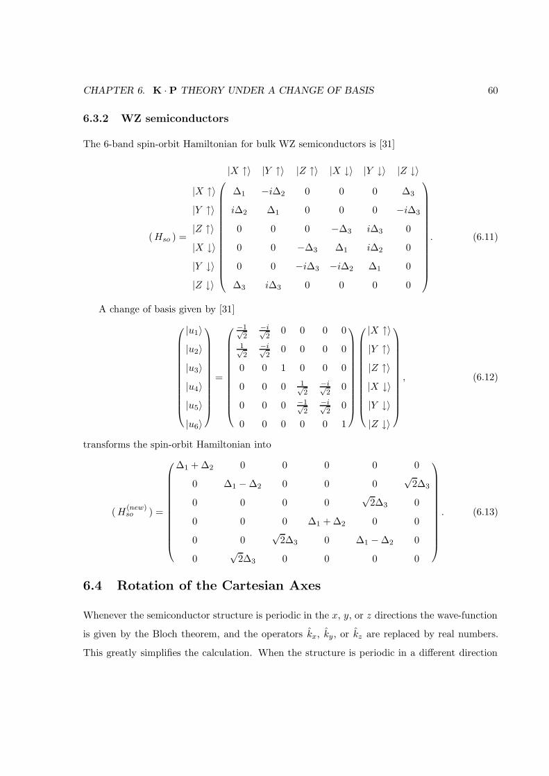
CHAPTER 6. K · P THEORY UNDER A CHANGE OF BASIS 60
6.3.2 WZ semiconductors
The 6-band spin-orbit Hamiltonian for bulk WZ semiconductors is [31]
(Hso ) =
|X ↑〉 |Y ↑〉 |Z ↑〉 |X ↓〉 |Y ↓〉 |Z ↓〉
|X ↑〉 ∆1 −i∆2 0 0 0 ∆3
|Y ↑〉 i∆2 ∆1 0 0 0 −i∆3
|Z ↑〉 0 0 0 −∆3 i∆3 0
|X ↓〉 0 0 −∆3 ∆1 i∆2 0
|Y ↓〉 0 0 −i∆3 −i∆2 ∆1 0
|Z ↓〉 ∆3 i∆3 0 0 0 0
. (6.11)
A change of basis given by [31]
|u1〉|u2〉|u3〉|u4〉|u5〉|u6〉
=
−1√2
−i√2
0 0 0 0
1√2
−i√2
0 0 0 0
0 0 1 0 0 0
0 0 0 1√2
−i√2
0
0 0 0 −1√2
−i√2
0
0 0 0 0 0 1
|X ↑〉|Y ↑〉|Z ↑〉|X ↓〉|Y ↓〉|Z ↓〉
, (6.12)
transforms the spin-orbit Hamiltonian into
(H(new)so ) =
∆1 + ∆2 0 0 0 0 0
0 ∆1 − ∆2 0 0 0√
2∆3
0 0 0 0√
2∆3 0
0 0 0 ∆1 + ∆2 0 0
0 0√
2∆3 0 ∆1 − ∆2 0
0√
2∆3 0 0 0 0
. (6.13)
6.4 Rotation of the Cartesian Axes
Whenever the semiconductor structure is periodic in the x, y, or z directions the wave-function
is given by the Bloch theorem, and the operators kx, ky, or kz are replaced by real numbers.
This greatly simplifies the calculation. When the structure is periodic in a different direction
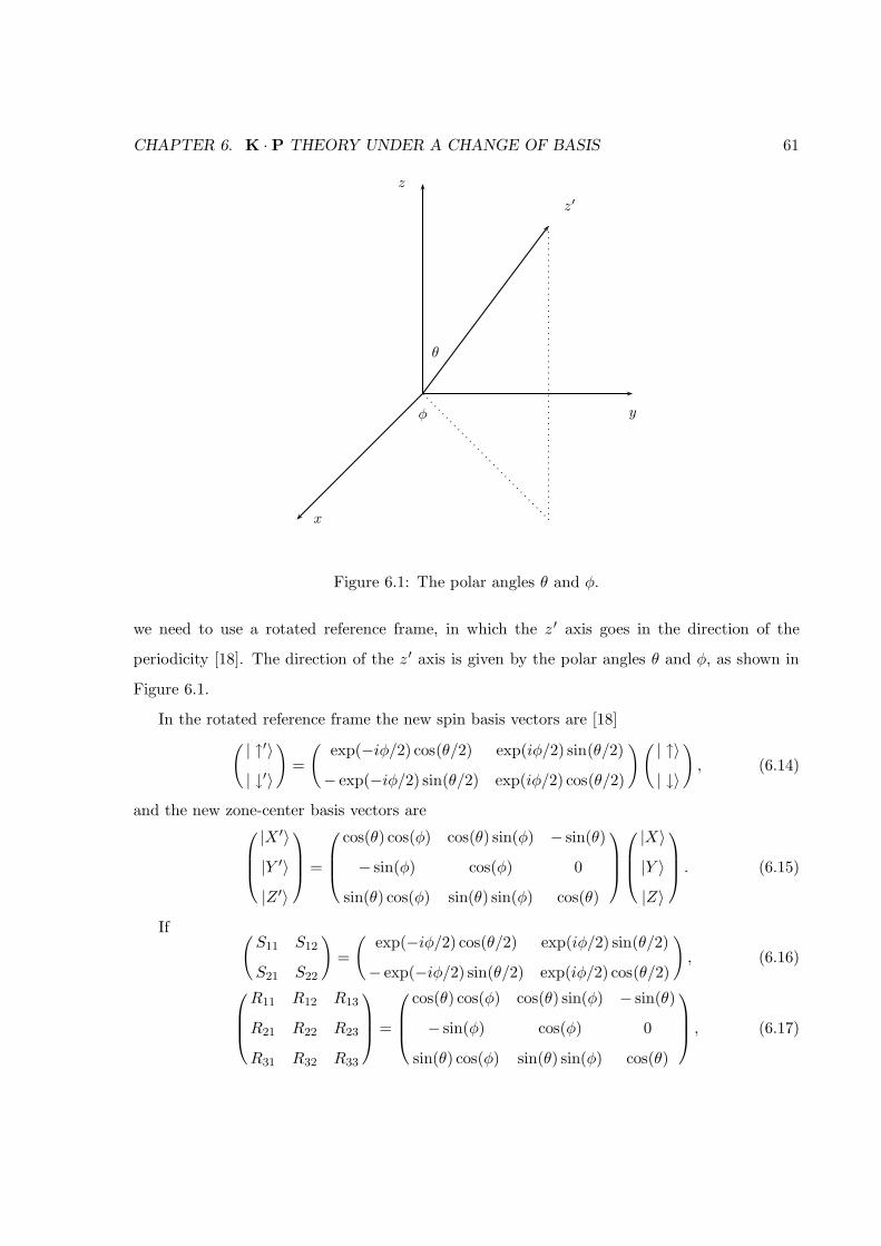
CHAPTER 6. K · P THEORY UNDER A CHANGE OF BASIS 61
z
y
x
z′
θ
φ
Figure 6.1: The polar angles θ and φ.
we need to use a rotated reference frame, in which the z ′ axis goes in the direction of the
periodicity [18]. The direction of the z ′ axis is given by the polar angles θ and φ, as shown in
Figure 6.1.
In the rotated reference frame the new spin basis vectors are [18]
( | ↑′〉| ↓′〉
)=
(exp(−iφ/2) cos(θ/2) exp(iφ/2) sin(θ/2)
− exp(−iφ/2) sin(θ/2) exp(iφ/2) cos(θ/2)
)( | ↑〉| ↓〉
), (6.14)
and the new zone-center basis vectors are
|X ′〉|Y ′〉|Z ′〉
=
cos(θ) cos(φ) cos(θ) sin(φ) − sin(θ)
− sin(φ) cos(φ) 0
sin(θ) cos(φ) sin(θ) sin(φ) cos(θ)
|X〉|Y 〉|Z〉
. (6.15)
If (S11 S12
S21 S22
)=
(exp(−iφ/2) cos(θ/2) exp(iφ/2) sin(θ/2)
− exp(−iφ/2) sin(θ/2) exp(iφ/2) cos(θ/2)
), (6.16)
R11 R12 R13
R21 R22 R23
R31 R32 R33
=
cos(θ) cos(φ) cos(θ) sin(φ) − sin(θ)
− sin(φ) cos(φ) 0
sin(θ) cos(φ) sin(θ) sin(φ) cos(θ)
, (6.17)
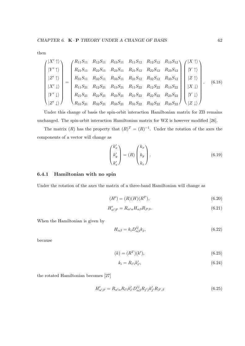
CHAPTER 6. K · P THEORY UNDER A CHANGE OF BASIS 62
then
|X ′ ↑〉|Y ′ ↑〉|Z ′ ↑〉|X ′ ↓〉|Y ′ ↓〉|Z ′ ↓〉
=
R11S11 R12S11 R13S11 R11S12 R12S12 R13S12
R21S11 R22S11 R23S11 R21S12 R22S12 R23S12
R31S11 R32S11 R33S11 R31S12 R32S12 R33S12
R11S21 R12S21 R13S21 R11S22 R12S22 R13S22
R21S21 R22S21 R23S21 R21S22 R22S22 R23S22
R31S21 R32S21 R33S21 R31S22 R32S22 R33S22
|X ↑〉|Y ↑〉|Z ↑〉|X ↓〉|Y ↓〉|Z ↓〉
. (6.18)
Under this change of basis the spin-orbit interaction Hamiltonian matrix for ZB remains
unchanged. The spin-orbit interaction Hamiltonian matrix for WZ is however modified [26].
The matrix (R) has the property that (R)T = (R)−1. Under the rotation of the axes the
components of a vector will change as
k′x
k′y
k′z
= (R)
kx
ky
kz
. (6.19)
6.4.1 Hamiltonian with no spin
Under the rotation of the axes the matrix of a three-band Hamiltonian will change as
(H ′) = (R)(H)(RT ), (6.20)
H ′α′β′ = Rα′αHαβRβ′β. (6.21)
When the Hamiltonian is given by
Hαβ = kiDijαβkj , (6.22)
because
(k) = (RT )(k′), (6.23)
ki = Ri′ik′i′ , (6.24)
the rotated Hamiltonian becomes [27]
H ′α′β′ = Rα′αRi′ik
′i′D
ijαβRj′jk
′j′Rβ′.β (6.25)
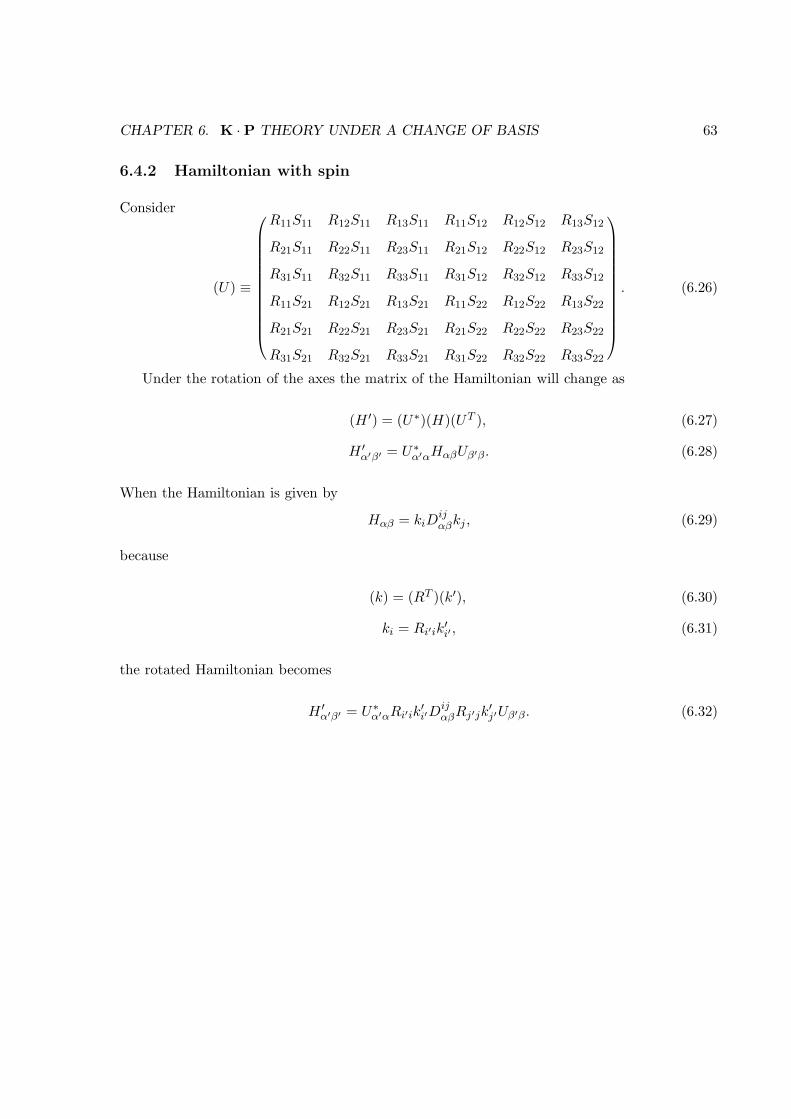
CHAPTER 6. K · P THEORY UNDER A CHANGE OF BASIS 63
6.4.2 Hamiltonian with spin
Consider
(U) ≡
R11S11 R12S11 R13S11 R11S12 R12S12 R13S12
R21S11 R22S11 R23S11 R21S12 R22S12 R23S12
R31S11 R32S11 R33S11 R31S12 R32S12 R33S12
R11S21 R12S21 R13S21 R11S22 R12S22 R13S22
R21S21 R22S21 R23S21 R21S22 R22S22 R23S22
R31S21 R32S21 R33S21 R31S22 R32S22 R33S22
. (6.26)
Under the rotation of the axes the matrix of the Hamiltonian will change as
(H ′) = (U∗)(H)(UT ), (6.27)
H ′α′β′ = U∗
α′αHαβUβ′β. (6.28)
When the Hamiltonian is given by
Hαβ = kiDijαβkj , (6.29)
because
(k) = (RT )(k′), (6.30)
ki = Ri′ik′i′ , (6.31)
the rotated Hamiltonian becomes
H ′α′β′ = U∗
α′αRi′ik′i′D
ijαβRj′jk
′j′Uβ′β. (6.32)
Chapter 7
Strain in Cylindrical
Heterostructures
7.1 Elasticity Theory in Cartesian Coordinates
The basic quantity in elasticity theory is the deformation vector field u = x ′ − x relating the
position x of a point before the deformation to the position x′ of the point after the deformation.
For a pair of two close points du = dx′ − dx, and the distance between the two points after the
deformation can be written as [61]
(dx′)2 = (dx)2 + 2εijdxidxj , (7.1)
where the symmetric strain tensor is defined as
εij =1
2
(∂ui
∂xj+∂uj
∂xi+∂uk
∂xi
∂uk
∂xj
). (7.2)
When the deformations are small the derivatives ∂ui/∂xj are small, and we keep only linear
terms in these derivatives. This is how we end up with the expression for the linear strain:
εij =1
2
(∂ui
∂xj+∂uj
∂xi
). (7.3)
The strain-displacement equations (7.3) can be integrated, to obtain the deformation from the
strain tensor. Since the six stress tensor components are more than the three displacement
64
CHAPTER 7. STRAIN IN CYLINDRICAL HETEROSTRUCTURES 65
components, extra conditions need to be imposed to make sure that the solution is consistent.
The displacement field at a given point does not depend on the integration path. Stokes theorem
is applied to the integrand, and the following compatibility conditions are obtained [62] :
∂
∂xl
[εik − xj
(∂εik∂xj
− ∂εjk∂xi
)]=
∂
∂xk
[εil − xj
(∂εil∂xj
− ∂εjl∂xi
)]. (7.4)
Consider a small volume element inside a solid body. There are two kind of forces acting on
this volume element: the body forces (e.g. gravity) and the surface tractions. The surface
tractions are the forces due to the remaining of the solid, acting on the small volume element at
its surface. Since the surface tractions act only at the surface, they must be given by a surface
integral, which is then converted to a volume integral:
Fi =
∮σikdfk =
∫∂σik
∂xkdV, (7.5)
where σik is the stress tensor. σikdfk is the Fi component of the force acting on a surface
element dfk perpendicular to the xk axis. For a body in rotational equilibrium the stress tensor
must be symmetric [61]. When the body is in translational motion the net force acting on the
volume element gives its acceleration:
∂σik
∂xk+ fi = ρai, (7.6)
where f is the body force density (e.g. ρg), ρ is the mass density, and a is the acceleration.
In general there is a proportionality relation between force and elongation (between stress and
strain), called Hooke’s Law. In the most general case this relation takes the form:
σij = Cijmnεmn, (7.7)
where Cijmn is the stiffness matrix. Although the 4 indices suggest 81 stiffness elements, due to
symmetry Cijmn = Cjimn and Cijmn = Cijnm. The existence of a strain energy density function,
when the system is adiabatic or isothermal, leads to Cijmn = Cmnij . As a result there are only
21 independent stiffness elements. For an isotropic material, due to symmetry considerations,
only 2 independent stiffness elements ( µ and λ ) are left. The stress-strain relations take the
form:
σij = 2µεij + λεnnδij . (7.8)
CHAPTER 7. STRAIN IN CYLINDRICAL HETEROSTRUCTURES 66
7.2 Elasticity Theory in Cylindrical Coordinates
In cylindrical coordinates the strain-displacement equations (7.3) take the form:
εrr =∂ur
∂r, (7.9)
εθθ =1
r
∂uθ
∂θ+ur
r, (7.10)
εzz =∂uz
∂z, (7.11)
εrθ =1
2
(1
r
∂ur
θ+∂uθ
∂r− uθ
r
), (7.12)
εrz =1
2
(∂ur
∂z+∂uz
∂r
), (7.13)
εθz =1
2
(∂uθ
∂z+
1
r
∂uz
∂θ
). (7.14)
The compatibility relations (7.4) take the form:
∂2εθθ
∂r2+
1
r2∂2εrr
∂θ2+
2
r
∂εθθ
∂r− 1
r
∂εrr
∂r= 2
(1
r
∂2εrθ
∂r∂θ+
1
r2∂εrθ
∂θ
), (7.15)
∂2εθθ
∂z2+
1
r2∂2εzz
∂θ2+
1
r
∂εzz
∂r= 2
(1
r
∂2εθz
∂z∂θ+
1
r
∂εzr
∂z
), (7.16)
∂2εzz
∂r2+∂2εrr
∂z2= 2
∂2εrz
∂z∂r, (7.17)
1
r
∂2εzz
∂r∂θ− 1
r2∂εzz
∂θ=
∂
∂z
(1
r
∂εzr
∂θ+∂εθz
∂r− ∂εrθ
∂z
)− ∂
∂z
(εθz
r
), (7.18)
1
r
∂2εrr
∂θ∂z=
∂
∂r
(1
r
∂εzr
∂θ− ∂εθz
∂r+∂εrθ
∂z
)− ∂
∂r
(εθz
r
)+
2
r
∂εrθ
∂z, (7.19)
∂2εθθ
∂r∂z− 1
r
∂εrr
∂z+
1
r
∂εθθ
∂z=
1
r
∂
∂θ
(−1
r
∂εzr
∂θ+∂εθz
∂r+∂εrθ
∂z
)+
1
r
∂
∂θ
(εθz
r
). (7.20)
The equilibrium relations (7.6) take the form:
∂σrr
∂r+
1
r
∂σθr
∂θ+∂σzr
∂z+
1
r(σrr − σθθ) + fr = ρar, (7.21)
∂σrθ
∂r+
1
r
∂σθθ
∂θ+∂σzθ
∂z+
2
rσrθ + fθ = ρaθ, (7.22)
∂σrz
∂r+
1
r
∂σθz
∂θ+∂σzz
∂z+
1
rσrz + fz = ρaz. (7.23)
The stress-strain relations (7.8) take the form:
σrr = 2µεrr + λ(εrr + εθθ + εzz), (7.24)
CHAPTER 7. STRAIN IN CYLINDRICAL HETEROSTRUCTURES 67
σθθ = 2µεθθ + λ(εrr + εθθ + εzz), (7.25)
σzz = 2µεzz + λ(εrr + εθθ + εzz), (7.26)
σrθ = 2µεrθ, (7.27)
σrz = 2µεrz, (7.28)
σθz = 2µεθz. (7.29)
7.3 Plane Deformation with Cylindrical Symmetry
A state of plane deformation is defined by ur = ur(r, θ), uθ = uθ(r, θ), uz = uz(z). If the
problem has cylindrical symmetry (no dependence on θ), and if there is no torsion (uθ = 0), the
deformation is given by ur = ur(r), uθ = 0, uz = uz(z). In this situation the strain-displacement
equations take the form:
εrr =∂ur
∂r, (7.30)
εθθ =ur
r, (7.31)
εzz =∂uz
∂z, (7.32)
εrθ = 0, (7.33)
εrz = 0, (7.34)
εθz = 0. (7.35)
The compatibility relations are reduced to:
∂2εθθ
∂r2+
2
r
∂εθθ
∂r− 1
r
∂εrr
∂r= 0. (7.36)
The stress-strain relations take the form:
σrr = 2µεrr + λ(εrr + εθθ + εzz), (7.37)
σθθ = 2µεθθ + λ(εrr + εθθ + εzz), (7.38)
σzz = 2µεzz + λ(εrr + εθθ + εzz), (7.39)
σrθ = 0, (7.40)
CHAPTER 7. STRAIN IN CYLINDRICAL HETEROSTRUCTURES 68
σrz = 0, (7.41)
σθz = 0. (7.42)
Suppose that the body is in translational equilibrium, and that there are no body forces. The
equilibrium relations take the form:
∂σrr
∂r+
1
r(σrr − σθθ) = 0, (7.43)
∂σzz
∂z= 0. (7.44)
Since∂σzz
∂z= (2µ+ λ)
∂εzz
∂z= 0, (7.45)
we conclude that εzz ≡ εo is constant, and that uz = εoz.
7.4 Infinite Embedded Cylindrical Wire with Cubic Structure
We are now ready to analyze the strain distribution in an infinitely long cylindrical wire em-
bedded in an infinite substrate. In the following the label ”in” refers to the wire, and the
label ”out” refers to the substrate. Let’s start with the wire and the substrate separated and
unstrained, as shown in Figure 7.1. The radius of the unstrained wire is greater than the radius
of the hole in the unstrained substrate. This difference is called δ. Because ε(out)zz at infinity is
zero, and because it is constant, we conclude that ε(out)zz = 0. The wire is first compressed, in
such a way as to preserve the cubic structure, until the lattice constant of the wire matches the
lattice constant of the substrate. Therefore
δ
ro=uz
z= εo =
a(out) − a(in)
a(out). (7.46)
The compressed wire is then inserted into the cavity, and the radial strain in allowed to relax.
This procedure is known as ”shrink fit” [63]. As a result the wire will end up with a deformation
u(in)r (r) and the substrate will end up with a deformation u
(out)r (r). It is clear from the figure
that
u(in)r (ro) − u(out)
r (ro) = δ. (7.47)

CHAPTER 7. STRAIN IN CYLINDRICAL HETEROSTRUCTURES 69
δ
Figure 7.1: The wire and the substrate before embedding.
u(out)r (ro)
u(in)r (ro)
ro
Figure 7.2: The wire and the substrate after the ”shrink fit” embedding. The shaded regions
are the compressed wire before insertion (right) and the relaxed wire after insertion (left).
CHAPTER 7. STRAIN IN CYLINDRICAL HETEROSTRUCTURES 70
The equation (7.47) is used to determine the pressure P at the wire-substrate interface, the key
to solving the strain distribution.
In a first step we substitute the stress components from (7.37) and (7.38) into (7.43).
2µ∂εrr
∂r+ λ
∂εrr
∂r+ λ
∂εθθ
∂r+
2µ
r(εrr − εθθ). (7.48)
In a second step we substitute the strain components from (7.30) and (7.31) into (7.48).
∂2ur
∂r2+
1
r
∂ur
∂r− ur
r2= 0. (7.49)
The general solution of the equation (7.49) is
ur(r) = C1r +C2
r. (7.50)
7.4.1 The Wire
In the wire C2 = 0, to prevent the divergence when the radius is zero. Therefore:
ur = C1r, (7.51)
εrr = C1, (7.52)
εθθ = C1, (7.53)
σrr = 2(µ+ λ)C1 + λεo. (7.54)
At the wire-substrate interface the radial stress is the negative pressure. This is the boundary
condition.
−P = 2(µ+ λ)C1 + λεo. (7.55)
As a consequence:
C1 = − P + λεo2(µ+ λ)
, (7.56)
u(in)r (r) = − P + λεo
2(µ+ λ)r. (7.57)
CHAPTER 7. STRAIN IN CYLINDRICAL HETEROSTRUCTURES 71
7.4.2 The Substrate
In the substrate C1 = 0, to prevent the divergence when the radius goes to infinity. Therefore:
ur =C2
r, (7.58)
εrr = −C2
r2, (7.59)
εθθ =C2
r2, (7.60)
σrr = −2µC2
r2. (7.61)
At the wire-substrate interface the radial stress is the negative pressure. This is the boundary
condition.
−P = −2µC2
r2o. (7.62)
As a consequence:
C2 =Pr2o2µ
, (7.63)
u(out)r (r) =
Pr2o2µr
. (7.64)
7.4.3 The Shrink Fit
We now substitute (7.57) and (7.64) into (7.47). For simplicity we assume that µ and λ are the
same in both materials [32].
− P + λεo2(µ+ λ)
ro −Pr2o2µro
= εoro. (7.65)
From (7.65) we find the pressure P , needed in (7.57) and (7.64) to give the strain distribution.
P = −εo(2µ+ 3λ)µ
2µ+ λ. (7.66)
Chapter 8
One-Band k · p Calculations -
Quantum Ice Cream Dot
8.1 Introduction
Modeling the electron states in semiconductor nanostructures remains a difficult computational
task. Various computational methods such as the transfer matrix method [64], the finite el-
ement method [65], the finite difference method [66, 67, 68], and the fast Fourier transform
technique [69] have been used. Other methods, the effective index method and numerical relax-
ation, have also been used to calculate the ground state of a cylindrical quantum dot (QD) [70].
The finite difference method (FDM) has been, by far, the most commonly used method. Never-
theless, implementation details are rarely given. One exception is in the study of GaN quantum
wells by Chuang and Chang [71].
The shape and size of a quantum dot determine the number of eigenstates and their degen-
eracy [72]. We investigated whether we can have a bound state in a very narrow quantum dot
with the shape of an ice cream cone (QIC dot). In this calculation the QIC dot is embedded
into a cube, with a potential barrier of 0.5 eV, as shown in Figure 8.1.
72
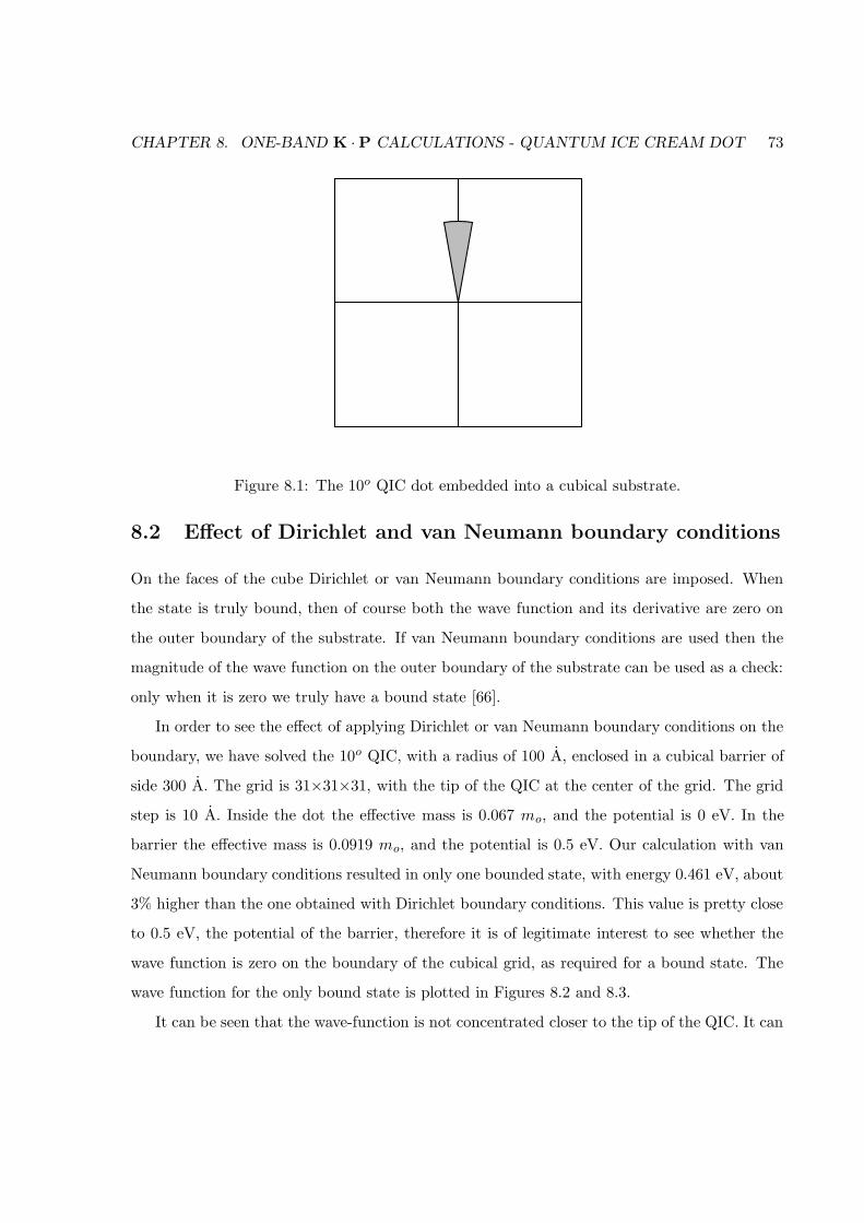
CHAPTER 8. ONE-BAND K ·P CALCULATIONS - QUANTUM ICE CREAM DOT 73
Figure 8.1: The 10o QIC dot embedded into a cubical substrate.
8.2 Effect of Dirichlet and van Neumann boundary conditions
On the faces of the cube Dirichlet or van Neumann boundary conditions are imposed. When
the state is truly bound, then of course both the wave function and its derivative are zero on
the outer boundary of the substrate. If van Neumann boundary conditions are used then the
magnitude of the wave function on the outer boundary of the substrate can be used as a check:
only when it is zero we truly have a bound state [66].
In order to see the effect of applying Dirichlet or van Neumann boundary conditions on the
boundary, we have solved the 10o QIC, with a radius of 100 A, enclosed in a cubical barrier of
side 300 A. The grid is 31×31×31, with the tip of the QIC at the center of the grid. The grid
step is 10 A. Inside the dot the effective mass is 0.067 mo, and the potential is 0 eV. In the
barrier the effective mass is 0.0919 mo, and the potential is 0.5 eV. Our calculation with van
Neumann boundary conditions resulted in only one bounded state, with energy 0.461 eV, about
3% higher than the one obtained with Dirichlet boundary conditions. This value is pretty close
to 0.5 eV, the potential of the barrier, therefore it is of legitimate interest to see whether the
wave function is zero on the boundary of the cubical grid, as required for a bound state. The
wave function for the only bound state is plotted in Figures 8.2 and 8.3.
It can be seen that the wave-function is not concentrated closer to the tip of the QIC. It can
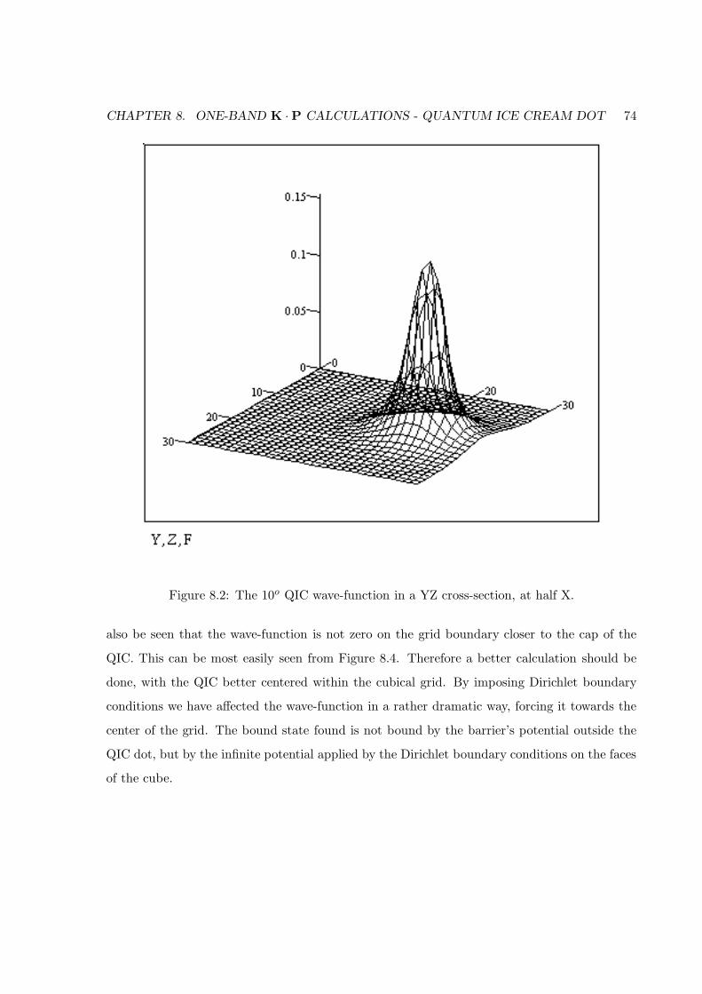
CHAPTER 8. ONE-BAND K ·P CALCULATIONS - QUANTUM ICE CREAM DOT 74
Figure 8.2: The 10o QIC wave-function in a YZ cross-section, at half X.
also be seen that the wave-function is not zero on the grid boundary closer to the cap of the
QIC. This can be most easily seen from Figure 8.4. Therefore a better calculation should be
done, with the QIC better centered within the cubical grid. By imposing Dirichlet boundary
conditions we have affected the wave-function in a rather dramatic way, forcing it towards the
center of the grid. The bound state found is not bound by the barrier’s potential outside the
QIC dot, but by the infinite potential applied by the Dirichlet boundary conditions on the faces
of the cube.
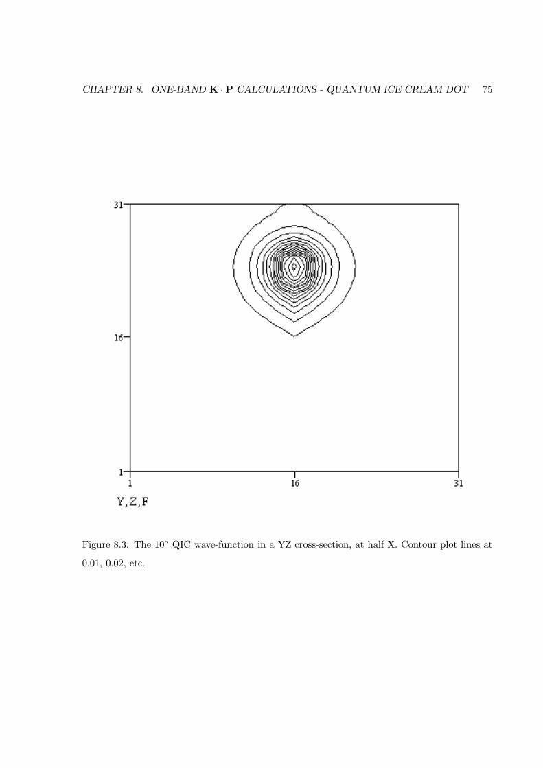
CHAPTER 8. ONE-BAND K ·P CALCULATIONS - QUANTUM ICE CREAM DOT 75
Figure 8.3: The 10o QIC wave-function in a YZ cross-section, at half X. Contour plot lines at
0.01, 0.02, etc.
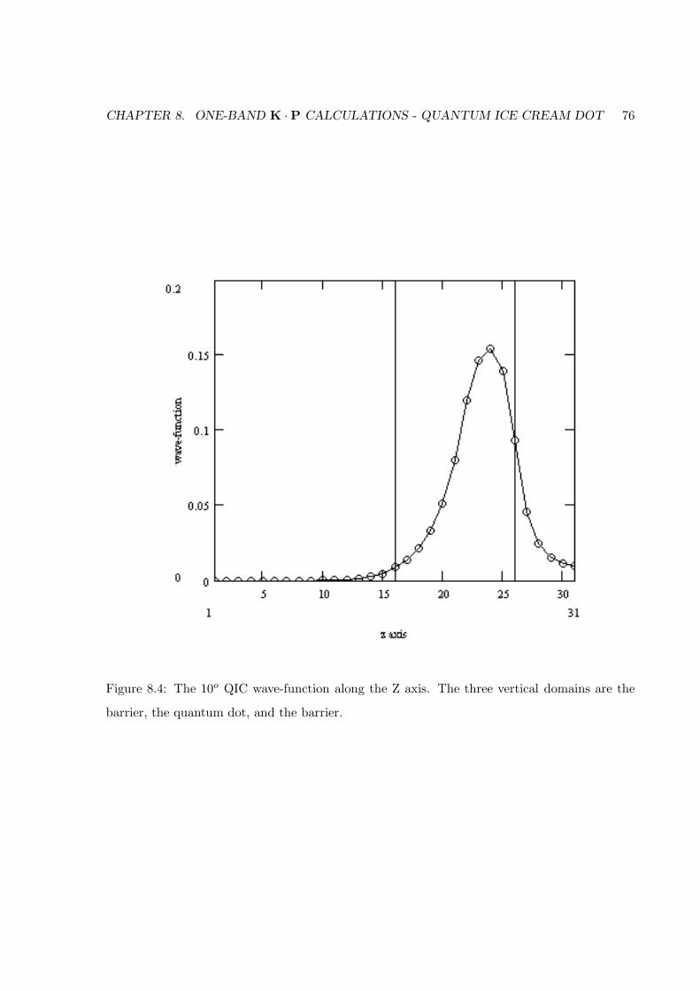
CHAPTER 8. ONE-BAND K ·P CALCULATIONS - QUANTUM ICE CREAM DOT 76
Figure 8.4: The 10o QIC wave-function along the Z axis. The three vertical domains are the
barrier, the quantum dot, and the barrier.
Chapter 9
One-Band k · p Calculations -
Elliptical Dot
9.1 Introduction
There are 11 coordinate systems with orthogonal coordinate lines [73]. Depending on the
symmetry of the domain, and also on the boundary conditions, the Schrodinger equation can or
cannot be simplified and solved exactly in the coordinate system compatible with the symmetry
of the quantum dot. The separability of the Schrodinger equation is very important when
studying shape effects, for it allows us to better understand why we get degeneracies in the
eigenfunctions [72].
In a recent paper [35], it is stated that the two-dimensional elliptic quantum dot (QD)
problem with finite barrier can be exactly solved. The purpose of our work [34] is to point out
that the above assertion is incorrect and to correct the energy spectra presented in Ref. [35].
9.2 The Eigenstates of an Elliptical Quantum Dot
The separation of the Schrodinger equation for an elliptic QD in elliptical coordinates leads to
the Mathieu and modified Mathieu differential equations (Eqs. (3a) and (3b) of Ref. [35]). For
the infinite barrier problem, it is correctly stated that the energy eigenvalues E are determined
77
CHAPTER 9. ONE-BAND K ·P CALCULATIONS - ELLIPTICAL DOT 78
by the boundary condition imposed upon the even or odd radial Mathieu functions
Mc(1)l (c, q1, U) = 0, (9.1)
Ms(1)l (c, q1, U) = 0, (9.2)
where c is a separation constant, q1 = f2k2/4 with f =√a2 − b2 the focal length and k2 =
2m∗E/h2, and U = arctanh(b/a) is the dot boundary. Periodicity of the angular Mathieu
function determines the separation constant c, while the zeroes of the radial Mathieu function
at u = U determine the energy eigenvalues [73].
For the finite barrier problem the even and odd wave functions (Eqs. (11) and (12) of
Ref. [35]) are assumed to have the form
Ψen,l(u, v)
=
N e
n,lMc(1)l (u, q1n,l
)cel(v, q1n,l), u ≤ U,
N en,lMc
(3)l (u,−q2n,l
)cel(v,−q2n,l), u > U,
(9.3)
and
Ψon,l(u, v)
=
No
n,lMs(1)l (u, q1n,l
)sel(v, q1n,l), u ≤ U,
Non,lMs
(3)l (u,−q2n,l
)sel(v,−q2n,l), u > U.
(9.4)
These functions lead to a simple boundary condition (Eq. (5) of Ref. [35]), which is solved
similarly to the infinite barrier case.
That the wave functions (3) and (4) cannot be right can be seen by rewriting the continuity
of the wave function on the ellipse boundary. For example, Eq. (3) gives
cel(v, q1n,l) =
Mc(3)l (U,−q2n,l
)
Mc(1)l (U,q1n,l
)cel(v,−q2n,l
)
≡ constant × cel(v,−q2n,l). (9.5)
The latter equation cannot be satisfied for an arbitrary v. If the angular Mathieu functions
were the same for all v (apart from a proportionality constant) then, in particular, the following
CHAPTER 9. ONE-BAND K ·P CALCULATIONS - ELLIPTICAL DOT 79
set of equations would be fulfilled:
cl,q1 − 2q1 cos(2v) =1
cel(v, q1)
d2cel(v, q1)
dv2
=1
cel(v,−q2)d2cel(v,−q2)
dv2= cl,−q2 − 2q2 cos(2v). (9.6)
From Eq. (9.6) it follows that:
2(q1 − q2) cos(2v) = cl,q1 − cl,−q2 . (9.7)
The latter equation cannot be fulfilled for all v since q1 − q2 = f2m∗Vo/(2h2) 6= 0. The origin
of the problem is, obviously, that the problem is not separable, contrary to what is stated in
Ref. [35].
The correct wave function for the finite barrier problem can be written in the form (for the
even states as example)
Ψen(u, v)
=
∑lA
en,lMc
(1)l (u, q1n)cel(v, q1n), u ≤ U,
∑lB
en,lMc
(3)l (u,−q2n)cel(v,−q2n), u > U.
(9.8)
In addition to the summation, we note that the q’s should not be functions of l.
In the absence of a simple exact solution, we present a numerical solution. We have used
the finite-difference method on a 400 × 400 uniform rectangular grid. Different eccentricities
have been achieved by changing the mesh sizes in the two directions. The algebraic eigenvalue
problem for the resulting large sparse matrix has been solved with the help of the ARPACK
library [74]. For the infinite-barrier problem, we have obtained a spectrum identical to Fig. 5
of Ref. [35]. However, for a finite barrier, our results are different. For example, we have
reproduced in our Fig. 9.1, results of our calculations corresponding to Fig. 3 of Ref. [35].
While we get the same limiting eigenvalues for the circular dot (due to the separability of
the problem), our results differ for increasing eccentricity. In particular, we get a more rapid
increase in the energies with increasing eccentricity. This is the same trend seen for the infinite
barrier QD.
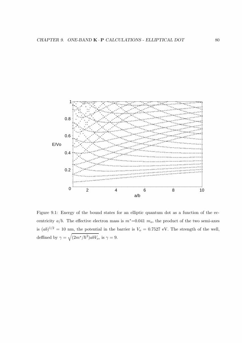
CHAPTER 9. ONE-BAND K ·P CALCULATIONS - ELLIPTICAL DOT 80
0
0.2
0.4
0.6
0.8
1
E/Vo
2 4 6 8 10a/b
Figure 9.1: Energy of the bound states for an elliptic quantum dot as a function of the ec-
centricity a/b. The effective electron mass is m∗=0.041 mo, the product of the two semi-axes
is (ab)1/2 = 10 nm, the potential in the barrier is Vo = 0.7527 eV. The strength of the well,
deffined by γ =√
(2m∗/h2)abVo, is γ = 9.
Chapter 10
One-Band k · p Calculations -
Nanowire Superlattice
10.1 Introduction
In this chapter we apply the finite difference method in cylindrical polar coordinates to solve
the Schrodinger equation for a nanowire superlattice. Our work [36] is motivated by two recent
sets of papers. In the first one, most of which were published in Comp. Phys. Comm., various
authors have applied the FDM in cylindrical polar coordinates (CPC) to study quantum dots
using the one-band effective mass equation [75, 76, 77], but details of the FDM were not given.
In particular, complications of the formulation near the cylinder axis were not mentioned. In
the second one, there has been a flurry of experimental activity on the growth of free-standing
semiconductor nanowire superlattices (NWSL’s) [37, 38, 78, 79, 80]. These NWSL are charac-
terized by a cylindrical cross-section, a periodicity along the cylinder axis, and an effectively
infinite potential barrier for the electrons outside the wire. Extremely polarized photolumines-
cence is one characteristic that makes NWSL likely candidates for practical applications. In
addition, a recent one-dimensional theory predicted the remarkable existence of an inversion
regime when the localization of the electron states can be reversed [39].
Our central goal is to demonstrate the applicability of the FDM in CPC for the novel study
of NWSL’s. FDM in CPC is needed since using the admitted more flexible Cartesian system will
81
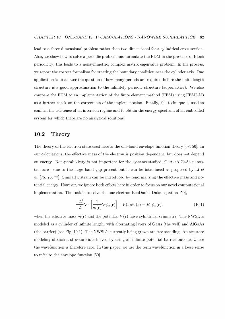
CHAPTER 10. ONE-BAND K · P CALCULATIONS - NANOWIRE SUPERLATTICE 82
lead to a three-dimensional problem rather than two-dimensional for a cylindrical cross-section.
Also, we show how to solve a periodic problem and formulate the FDM in the presence of Bloch
periodicity; this leads to a nonsymmetric, complex matrix eigenvalue problem. In the process,
we report the correct formalism for treating the boundary condition near the cylinder axis. One
application is to answer the question of how many periods are required before the finite-length
structure is a good approximation to the infinitely periodic structure (superlattice). We also
compare the FDM to an implementation of the finite element method (FEM) using FEMLAB
as a further check on the correctness of the implementation. Finally, the technique is used to
confirm the existence of an inversion regime and to obtain the energy spectrum of an embedded
system for which there are no analytical solutions.
10.2 Theory
The theory of the electron state used here is the one-band envelope function theory [68, 50]. In
our calculations, the effective mass of the electron is position dependent, but does not depend
on energy. Non-parabolicity is not important for the systems studied, GaAs/AlGaAs nanos-
tructures, due to the large band gap present but it can be introduced as proposed by Li et
al. [75, 76, 77]. Similarly, strain can be introduced by renormalizing the effective mass and po-
tential energy. However, we ignore both effects here in order to focus on our novel computational
implementation. The task is to solve the one-electron BenDaniel-Duke equation [50],
−h2
2∇ ·
[1
m(r)∇ψn(r)
]+ V (r)ψn(r) = Enψn(r), (10.1)
when the effective mass m(r) and the potential V (r) have cylindrical symmetry. The NWSL is
modeled as a cylinder of infinite length, with alternating layers of GaAs (the well) and AlGaAs
(the barrier) (see Fig. 10.1). The NWSL’s currently being grown are free standing. An accurate
modeling of such a structure is achieved by using an infinite potential barrier outside, where
the wavefunction is therefore zero. In this paper, we use the term wavefunction in a loose sense
to refer to the envelope function [50].
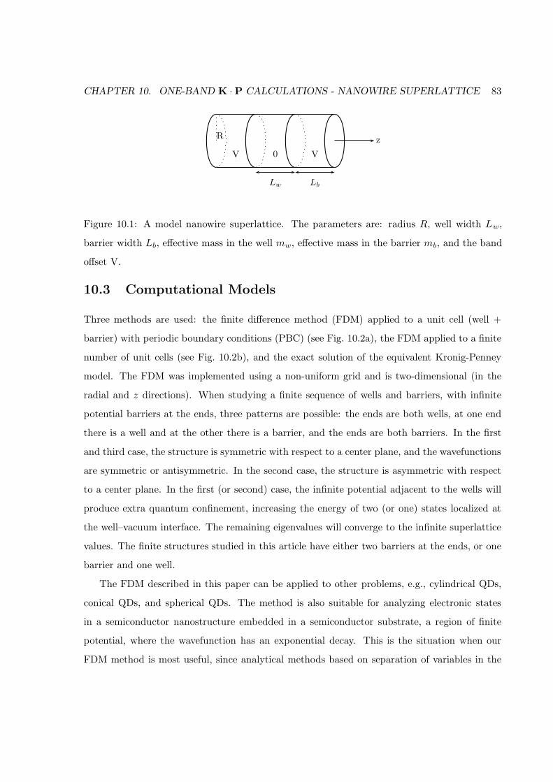
CHAPTER 10. ONE-BAND K · P CALCULATIONS - NANOWIRE SUPERLATTICE 83
Rz
V 0 V
Lw Lb
Figure 10.1: A model nanowire superlattice. The parameters are: radius R, well width Lw,
barrier width Lb, effective mass in the well mw, effective mass in the barrier mb, and the band
offset V.
10.3 Computational Models
Three methods are used: the finite difference method (FDM) applied to a unit cell (well +
barrier) with periodic boundary conditions (PBC) (see Fig. 10.2a), the FDM applied to a finite
number of unit cells (see Fig. 10.2b), and the exact solution of the equivalent Kronig-Penney
model. The FDM was implemented using a non-uniform grid and is two-dimensional (in the
radial and z directions). When studying a finite sequence of wells and barriers, with infinite
potential barriers at the ends, three patterns are possible: the ends are both wells, at one end
there is a well and at the other there is a barrier, and the ends are both barriers. In the first
and third case, the structure is symmetric with respect to a center plane, and the wavefunctions
are symmetric or antisymmetric. In the second case, the structure is asymmetric with respect
to a center plane. In the first (or second) case, the infinite potential adjacent to the wells will
produce extra quantum confinement, increasing the energy of two (or one) states localized at
the well–vacuum interface. The remaining eigenvalues will converge to the infinite superlattice
values. The finite structures studied in this article have either two barriers at the ends, or one
barrier and one well.
The FDM described in this paper can be applied to other problems, e.g., cylindrical QDs,
conical QDs, and spherical QDs. The method is also suitable for analyzing electronic states
in a semiconductor nanostructure embedded in a semiconductor substrate, a region of finite
potential, where the wavefunction has an exponential decay. This is the situation when our
FDM method is most useful, since analytical methods based on separation of variables in the
CHAPTER 10. ONE-BAND K · P CALCULATIONS - NANOWIRE SUPERLATTICE 84
O z
ρ
vacuum∞
well0
barrierV
(a)
O z
ρ
vacuum∞
V 0 V 0 V
(b)
Figure 10.2: The domain for (a) a unit cell with periodic boundary conditions and (b) a finite
number of unit cells, with barrier layers at both ends.
BenDaniel-Duke equation do not apply.
For a planar superlattice of finite length, Kolbas and Holonyak have developed a transfer
matrix method (TMM) [81]. The TMM can also be applied for a cylindrical superlattice of
finite length, provided it is surrounded by vacuum. In the TMM method, the first and last
barrier regions are extended to infinity, which gives a slightly different structure from the one
studied here. We also note that they used an incorrect boundary condition, though this is not
expected to impact the numerical convergence.
10.4 FDM applied to a unit cell with PBC
This method has the advantage of a smaller grid and, therefore, significantly reduced memory
and computing time requirements. The disadvantage is the presence of complex numbers in the
Hamiltonian matrix, due to the use of Bloch’s theorem.
We write the gradient and the divergence operators in cylindrical coordinates. The BenDaniel-
Duke equation, Eq. (10.1), becomes
−h2
2
[1
ρ
1
m
∂ψ
∂ρ+
∂
∂ρ
(1
m
∂ψ
∂ρ
)+
1
ρ
∂
∂φ
(1
m
1
ρ
∂ψ
∂φ
)+
∂
∂z
(1
m
∂ψ
∂z
)](10.2)
+V ψ = Eψ.
Due to the cylindrical symmetry, V = V (ρ, z), m = m(ρ, z), and ψ = F (ρ, z)eiLφ. The
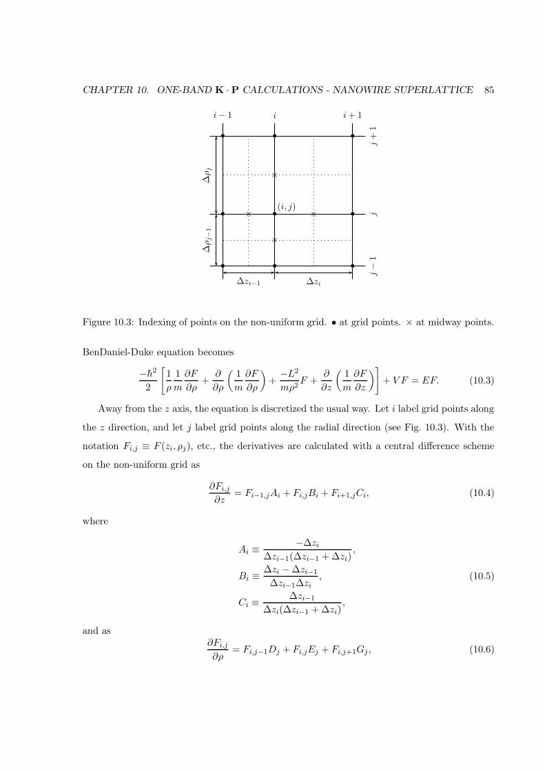
CHAPTER 10. ONE-BAND K · P CALCULATIONS - NANOWIRE SUPERLATTICE 85
∆zi−1 ∆zi
∆ρ
j−
1∆
ρj
i − 1 i i + 1
j−
1j
j+
1
•
•
•
•
•
•
•
•
•
×
×
× ×
(i, j)
Figure 10.3: Indexing of points on the non-uniform grid. • at grid points. × at midway points.
BenDaniel-Duke equation becomes
−h2
2
[1
ρ
1
m
∂F
∂ρ+
∂
∂ρ
(1
m
∂F
∂ρ
)+
−L2
mρ2F +
∂
∂z
(1
m
∂F
∂z
)]+ V F = EF. (10.3)
Away from the z axis, the equation is discretized the usual way. Let i label grid points along
the z direction, and let j label grid points along the radial direction (see Fig. 10.3). With the
notation Fi,j ≡ F (zi, ρj), etc., the derivatives are calculated with a central difference scheme
on the non-uniform grid as
∂Fi,j
∂z= Fi−1,jAi + Fi,jBi + Fi+1,jCi, (10.4)
where
Ai ≡−∆zi
∆zi−1(∆zi−1 + ∆zi),
Bi ≡∆zi − ∆zi−1
∆zi−1∆zi, (10.5)
Ci ≡∆zi−1
∆zi(∆zi−1 + ∆zi),
and as∂Fi,j
∂ρ= Fi,j−1Dj + Fi,jEj + Fi,j+1Gj , (10.6)
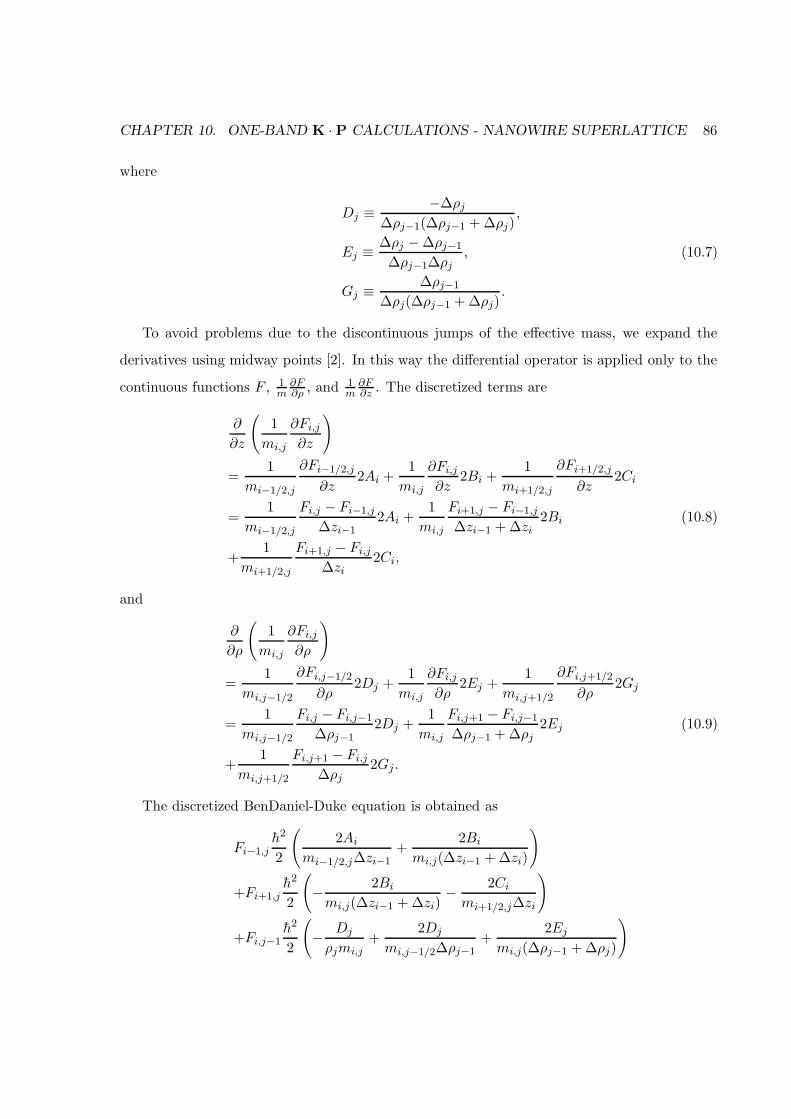
CHAPTER 10. ONE-BAND K · P CALCULATIONS - NANOWIRE SUPERLATTICE 86
where
Dj ≡−∆ρj
∆ρj−1(∆ρj−1 + ∆ρj),
Ej ≡∆ρj − ∆ρj−1
∆ρj−1∆ρj, (10.7)
Gj ≡ ∆ρj−1
∆ρj(∆ρj−1 + ∆ρj).
To avoid problems due to the discontinuous jumps of the effective mass, we expand the
derivatives using midway points [2]. In this way the differential operator is applied only to the
continuous functions F , 1m
∂F∂ρ , and 1
m∂F∂z . The discretized terms are
∂
∂z
(1
mi,j
∂Fi,j
∂z
)
=1
mi−1/2,j
∂Fi−1/2,j
∂z2Ai +
1
mi,j
∂Fi,j
∂z2Bi +
1
mi+1/2,j
∂Fi+1/2,j
∂z2Ci
=1
mi−1/2,j
Fi,j − Fi−1,j
∆zi−12Ai +
1
mi,j
Fi+1,j − Fi−1,j
∆zi−1 + ∆zi2Bi (10.8)
+1
mi+1/2,j
Fi+1,j − Fi,j
∆zi2Ci,
and
∂
∂ρ
(1
mi,j
∂Fi,j
∂ρ
)
=1
mi,j−1/2
∂Fi,j−1/2
∂ρ2Dj +
1
mi,j
∂Fi,j
∂ρ2Ej +
1
mi,j+1/2
∂Fi,j+1/2
∂ρ2Gj
=1
mi,j−1/2
Fi,j − Fi,j−1
∆ρj−12Dj +
1
mi,j
Fi,j+1 − Fi,j−1
∆ρj−1 + ∆ρj2Ej (10.9)
+1
mi,j+1/2
Fi,j+1 − Fi,j
∆ρj2Gj .
The discretized BenDaniel-Duke equation is obtained as
Fi−1,jh2
2
(2Ai
mi−1/2,j∆zi−1+
2Bi
mi,j(∆zi−1 + ∆zi)
)
+Fi+1,jh2
2
(− 2Bi
mi,j(∆zi−1 + ∆zi)− 2Ci
mi+1/2,j∆zi
)
+Fi,j−1h2
2
(− Dj
ρjmi,j+
2Dj
mi,j−1/2∆ρj−1+
2Ej
mi,j(∆ρj−1 + ∆ρj)
)
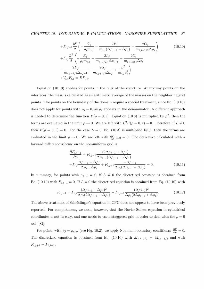
CHAPTER 10. ONE-BAND K · P CALCULATIONS - NANOWIRE SUPERLATTICE 87
+Fi,j+1h2
2
(− Gj
ρjmi,j− 2Ej
mi,j(∆ρj−1 + ∆ρj)− 2Gj
mi,j+1/2∆ρj
)(10.10)
+Fi,jh2
2
(− Ej
ρjmi,j− 2Ai
mi−1/2,j∆zi−1+
2Ci
mi+1/2,j∆zi
− 2Dj
mi,j−1/2∆ρj−1+
2Gj
mi,j+1/2∆ρj+
L2
mi,jρ2j
)
+Vi,jFi,j = EFi,j .
Equation (10.10) applies for points in the bulk of the structure. At midway points on the
interfaces, the mass is calculated as an arithmetic average of the masses on the neighboring grid
points. The points on the boundary of the domain require a special treatment, since Eq. (10.10)
does not apply for points with ρj = 0, as ρj appears in the denominator. A different approach
is needed to determine the function F (ρ = 0, z). Equation (10.3) is multiplied by ρ2, then the
terms are evaluated in the limit ρ→ 0. We are left with L2F (ρ = 0, z) = 0. Therefore, if L 6= 0
then F (ρ = 0, z) = 0. For the case L = 0, Eq. (10.3) is multiplied by ρ, then the terms are
evaluated in the limit ρ → 0. We are left with ∂F∂ρ |ρ=0 = 0. The derivative calculated with a
forward difference scheme on the non-uniform grid is
∂Fi,j−1
∂ρ= Fi,j−1
−(2∆ρj−1 + ∆ρj)
∆ρj−1(∆ρj−1 + ∆ρj)
+Fi,j∆ρj−1 + ∆ρj
∆ρj−1∆ρj+ Fi,j+1
−∆ρj−1
∆ρj(∆ρj−1 + ∆ρj)= 0. (10.11)
In summary, for points with ρj−1 = 0, if L 6= 0 the discretized equation is obtained from
Eq. (10.10) with Fi,j−1 = 0. If L = 0 the discretized equation is obtained from Eq. (10.10) with
Fi,j−1 = Fi,j(∆ρj−1 + ∆ρj)
2
∆ρj(2∆ρj−1 + ∆ρj)− Fi,j+1
(∆ρj−1)2
∆ρj(2∆ρj−1 + ∆ρj). (10.12)
The above treatment of Schrodinger’s equation in CPC does not appear to have been previously
reported. For completeness, we note, however, that the Navier-Stokes equation in cylindrical
coordinates is not as easy, and one needs to use a staggered grid in order to deal with the ρ = 0
axis [82].
For points with ρj = ρmax (see Fig. 10.2), we apply Neumann boundary conditions: ∂F∂ρ = 0.
The discretized equation is obtained from Eq. (10.10) with Mi,j+1/2 = Mi,j−1/2 and with
Fi,j+1 = Fi,j−1.
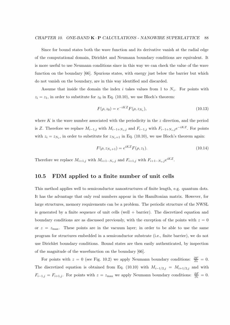
CHAPTER 10. ONE-BAND K · P CALCULATIONS - NANOWIRE SUPERLATTICE 88
Since for bound states both the wave function and its derivative vanish at the radial edge
of the computational domain, Dirichlet and Neumann boundary conditions are equivalent. It
is more useful to use Neumann conditions since in this way we can check the value of the wave
function on the boundary [66]. Spurious states, with energy just below the barrier but which
do not vanish on the boundary, are in this way identified and discarded.
Assume that inside the domain the index i takes values from 1 to Nz. For points with
zi = z1, in order to substitute for z0 in Eq. (10.10), we use Bloch’s theorem:
F (ρ, z0) = e−iKZF (ρ, zNz ), (10.13)
where K is the wave number associated with the periodicity in the z direction, and the period
is Z. Therefore we replace Mi−1,j with Mi−1+Nz ,j and Fi−1,j with Fi−1+Nz ,je−iKZ . For points
with zi = zNz , in order to substitute for zNz+1 in Eq. (10.10), we use Bloch’s theorem again:
F (ρ, zNz+1) = eiKZF (ρ, z1). (10.14)
Therefore we replace Mi+1,j with Mi+1−Nz ,j and Fi+1,j with Fi+1−Nz ,jeiKZ .
10.5 FDM applied to a finite number of unit cells
This method applies well to semiconductor nanostructures of finite length, e.g. quantum dots.
It has the advantage that only real numbers appear in the Hamiltonian matrix. However, for
large structures, memory requirements can be a problem. The periodic structure of the NWSL
is generated by a finite sequence of unit cells (well + barrier). The discretized equation and
boundary conditions are as discussed previously, with the exception of the points with z = 0
or z = zmax. These points are in the vacuum layer; in order to be able to use the same
program for structures embedded in a semiconductor substrate (i.e., finite barrier), we do not
use Dirichlet boundary conditions. Bound states are then easily authenticated, by inspection
of the magnitude of the wavefunction on the boundary [66].
For points with z = 0 (see Fig. 10.2) we apply Neumann boundary conditions: ∂F∂z = 0.
The discretized equation is obtained from Eq. (10.10) with Mi−1/2,j = Mi+1/2,j and with
Fi−1,j = Fi+1,j . For points with z = zmax we apply Neumann boundary conditions: ∂F∂z = 0.
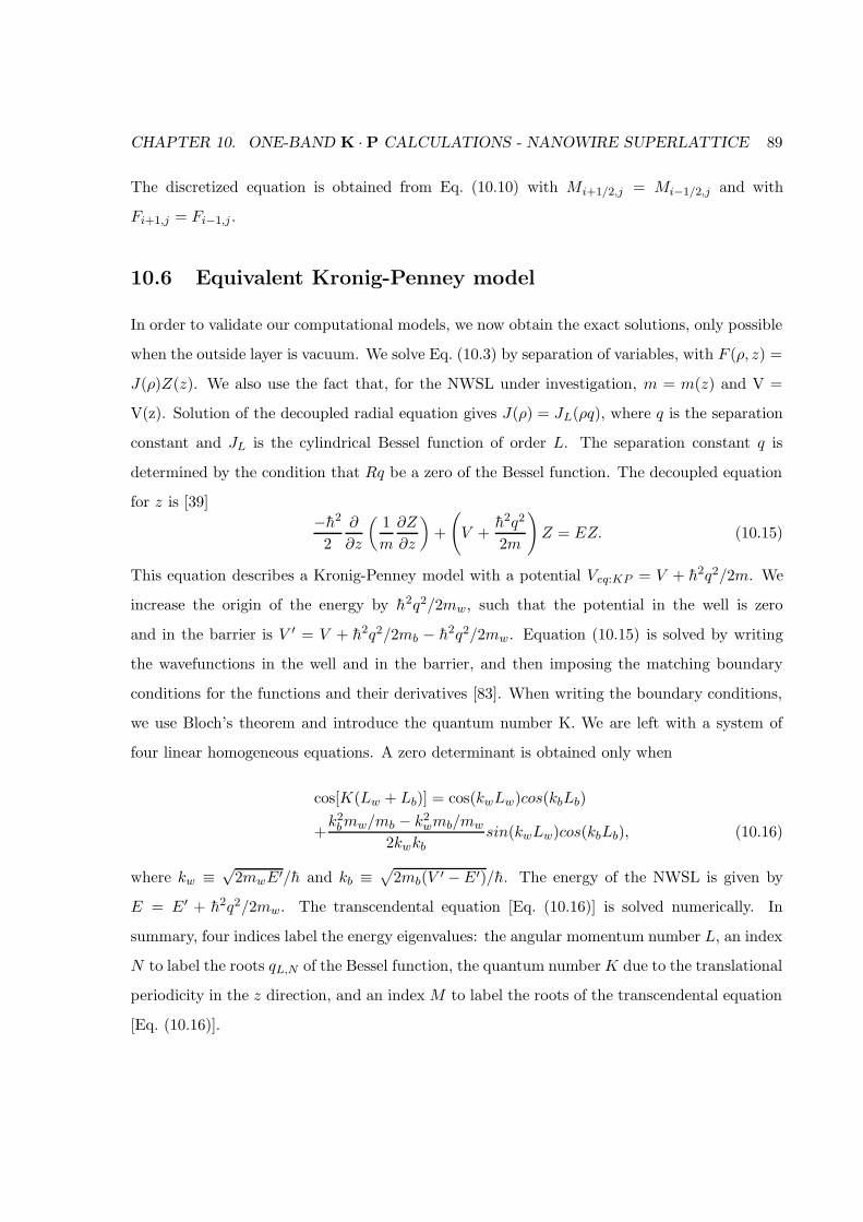
CHAPTER 10. ONE-BAND K · P CALCULATIONS - NANOWIRE SUPERLATTICE 89
The discretized equation is obtained from Eq. (10.10) with Mi+1/2,j = Mi−1/2,j and with
Fi+1,j = Fi−1,j .
10.6 Equivalent Kronig-Penney model
In order to validate our computational models, we now obtain the exact solutions, only possible
when the outside layer is vacuum. We solve Eq. (10.3) by separation of variables, with F (ρ, z) =
J(ρ)Z(z). We also use the fact that, for the NWSL under investigation, m = m(z) and V =
V(z). Solution of the decoupled radial equation gives J(ρ) = JL(ρq), where q is the separation
constant and JL is the cylindrical Bessel function of order L. The separation constant q is
determined by the condition that Rq be a zero of the Bessel function. The decoupled equation
for z is [39]
−h2
2
∂
∂z
(1
m
∂Z
∂z
)+
(V +
h2q2
2m
)Z = EZ. (10.15)
This equation describes a Kronig-Penney model with a potential Veq:KP = V + h2q2/2m. We
increase the origin of the energy by h2q2/2mw, such that the potential in the well is zero
and in the barrier is V ′ = V + h2q2/2mb − h2q2/2mw. Equation (10.15) is solved by writing
the wavefunctions in the well and in the barrier, and then imposing the matching boundary
conditions for the functions and their derivatives [83]. When writing the boundary conditions,
we use Bloch’s theorem and introduce the quantum number K. We are left with a system of
four linear homogeneous equations. A zero determinant is obtained only when
cos[K(Lw + Lb)] = cos(kwLw)cos(kbLb)
+k2
bmw/mb − k2wmb/mw
2kwkbsin(kwLw)cos(kbLb), (10.16)
where kw ≡√
2mwE′/h and kb ≡√
2mb(V ′ −E′)/h. The energy of the NWSL is given by
E = E′ + h2q2/2mw. The transcendental equation [Eq. (10.16)] is solved numerically. In
summary, four indices label the energy eigenvalues: the angular momentum number L, an index
N to label the roots qL,N of the Bessel function, the quantum numberK due to the translational
periodicity in the z direction, and an index M to label the roots of the transcendental equation
[Eq. (10.16)].
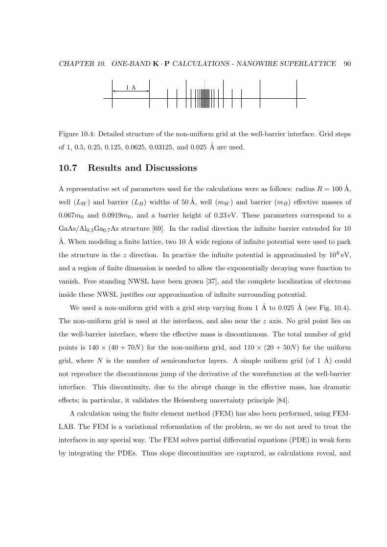
CHAPTER 10. ONE-BAND K · P CALCULATIONS - NANOWIRE SUPERLATTICE 90
1 A
Figure 10.4: Detailed structure of the non-uniform grid at the well-barrier interface. Grid steps
of 1, 0.5, 0.25, 0.125, 0.0625, 0.03125, and 0.025 A are used.
10.7 Results and Discussions
A representative set of parameters used for the calculations were as follows: radius R = 100 A,
well (LW ) and barrier (LB) widths of 50 A, well (mW ) and barrier (mB) effective masses of
0.067m0 and 0.0919m0, and a barrier height of 0.23 eV. These parameters correspond to a
GaAs/Al0.3Ga0.7As structure [69]. In the radial direction the infinite barrier extended for 10
A. When modeling a finite lattice, two 10 A wide regions of infinite potential were used to pack
the structure in the z direction. In practice the infinite potential is approximated by 106 eV,
and a region of finite dimension is needed to allow the exponentially decaying wave function to
vanish. Free standing NWSL have been grown [37], and the complete localization of electrons
inside these NWSL justifies our approximation of infinite surrounding potential.
We used a non-uniform grid with a grid step varying from 1 A to 0.025 A (see Fig. 10.4).
The non-uniform grid is used at the interfaces, and also near the z axis. No grid point lies on
the well-barrier interface, where the effective mass is discontinuous. The total number of grid
points is 140 × (40 + 70N) for the non-uniform grid, and 110 × (20 + 50N) for the uniform
grid, where N is the number of semiconductor layers. A simple uniform grid (of 1 A) could
not reproduce the discontinuous jump of the derivative of the wavefunction at the well-barrier
interface. This discontinuity, due to the abrupt change in the effective mass, has dramatic
effects; in particular, it validates the Heisenberg uncertainty principle [84].
A calculation using the finite element method (FEM) has also been performed, using FEM-
LAB. The FEM is a variational reformulation of the problem, so we do not need to treat the
interfaces in any special way. The FEM solves partial differential equations (PDE) in weak form
by integrating the PDEs. Thus slope discontinuities are captured, as calculations reveal, and
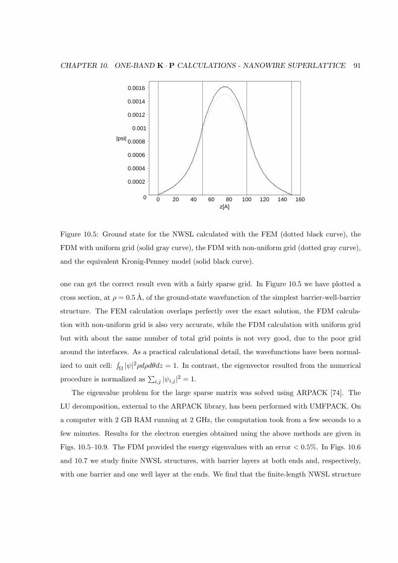
CHAPTER 10. ONE-BAND K · P CALCULATIONS - NANOWIRE SUPERLATTICE 91
0
0.0002
0.0004
0.0006
0.0008
0.001
0.0012
0.0014
0.0016
|psi|
0 20 40 60 80 100 120 140 160z[A]
Figure 10.5: Ground state for the NWSL calculated with the FEM (dotted black curve), the
FDM with uniform grid (solid gray curve), the FDM with non-uniform grid (dotted gray curve),
and the equivalent Kronig-Penney model (solid black curve).
one can get the correct result even with a fairly sparse grid. In Figure 10.5 we have plotted a
cross section, at ρ = 0.5 A, of the ground-state wavefunction of the simplest barrier-well-barrier
structure. The FEM calculation overlaps perfectly over the exact solution, the FDM calcula-
tion with non-uniform grid is also very accurate, while the FDM calculation with uniform grid
but with about the same number of total grid points is not very good, due to the poor grid
around the interfaces. As a practical calculational detail, the wavefunctions have been normal-
ized to unit cell:∫Ω |ψ|2ρdρdθdz = 1. In contrast, the eigenvector resulted from the numerical
procedure is normalized as∑
i,j |ψi,j |2 = 1.
The eigenvalue problem for the large sparse matrix was solved using ARPACK [74]. The
LU decomposition, external to the ARPACK library, has been performed with UMFPACK. On
a computer with 2 GB RAM running at 2 GHz, the computation took from a few seconds to a
few minutes. Results for the electron energies obtained using the above methods are given in
Figs. 10.5–10.9. The FDM provided the energy eigenvalues with an error < 0.5%. In Figs. 10.6
and 10.7 we study finite NWSL structures, with barrier layers at both ends and, respectively,
with one barrier and one well layer at the ends. We find that the finite-length NWSL structure
CHAPTER 10. ONE-BAND K · P CALCULATIONS - NANOWIRE SUPERLATTICE 92
0.1
0.12
0.14
0.16
0.18
0.2
0.22
E[eV]
2 4 6 8 10number of wells
Figure 10.6: Miniband formation in a symmetric NWSL structure. Energy levels as a function
of the number of wells. The segments on the right side are the energy bands for the infinite
NWSL, calculated with the FDM with non-uniform grid (left segments) and with the equivalent
Kronig-Penney model (right segments). L = 0, L = 1, and L = 2, in increasing order of the
energy.
with barrier layers at both ends approaches the superlattice energy bands when the number of
unit cells is of the order of 6. Note, however, that the infinite NWSL (with PBC) reproduces
the exact solution (given on the right-hand side) a lot faster.
The miniband formation in Fig. 10.6 can be understood from a perturbative point of view.
Indeed, consider the case of barriers of length much larger than the wells. In this situation
the wells are practically decoupled, and in each one we have the eigenstates of the single well.
As the length of the barriers is decreased, the states interact more strongly with each other,
and their energies shift, forming the miniband. It is clear that the number of states in one
miniband is equal to the number of wells in the superlattice structure. Each energy level of the
single well will correspond to a miniband in the infinite superlattice structure. The miniband
formation in Fig. 10.7 can be understood in the same way. Here, however, the state localized
at the well-vacuum interface is higher in energy, due to the increased quantum confinement,
and does not mix with the other states in the miniband. A similar state sandwiched between
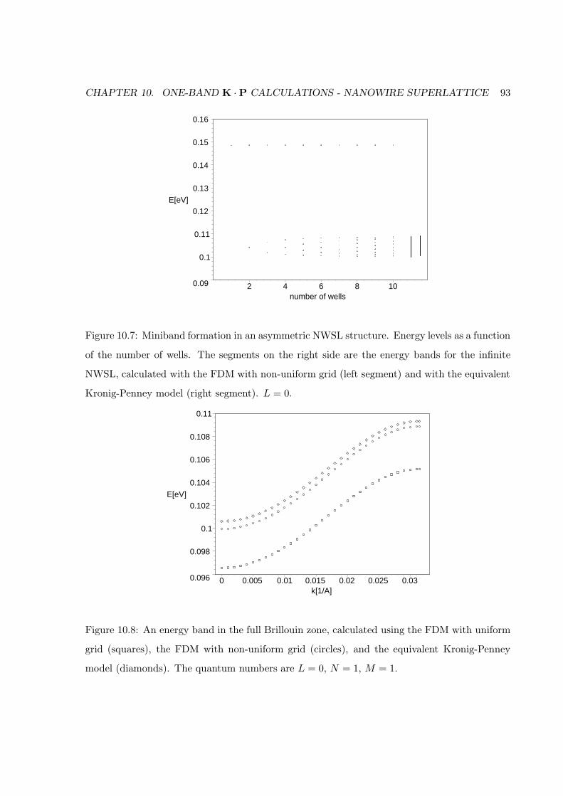
CHAPTER 10. ONE-BAND K · P CALCULATIONS - NANOWIRE SUPERLATTICE 93
0.09
0.1
0.11
0.12
0.13
0.14
0.15
0.16
E[eV]
2 4 6 8 10number of wells
Figure 10.7: Miniband formation in an asymmetric NWSL structure. Energy levels as a function
of the number of wells. The segments on the right side are the energy bands for the infinite
NWSL, calculated with the FDM with non-uniform grid (left segment) and with the equivalent
Kronig-Penney model (right segment). L = 0.
0.096
0.098
0.1
0.102
0.104
0.106
0.108
0.11
E[eV]
0 0.005 0.01 0.015 0.02 0.025 0.03k[1/A]
Figure 10.8: An energy band in the full Brillouin zone, calculated using the FDM with uniform
grid (squares), the FDM with non-uniform grid (circles), and the equivalent Kronig-Penney
model (diamonds). The quantum numbers are L = 0, N = 1, M = 1.
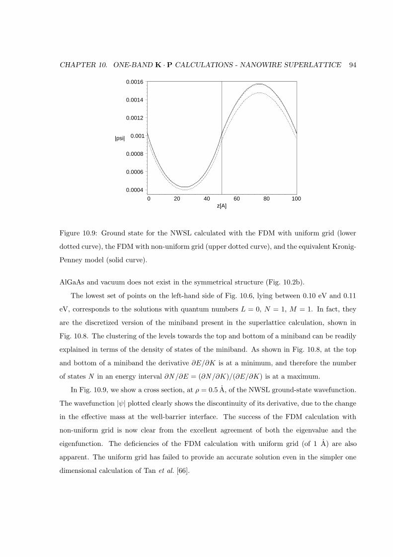
CHAPTER 10. ONE-BAND K · P CALCULATIONS - NANOWIRE SUPERLATTICE 94
0.0004
0.0006
0.0008
0.001
0.0012
0.0014
0.0016
|psi|
0 20 40 60 80 100z[A]
Figure 10.9: Ground state for the NWSL calculated with the FDM with uniform grid (lower
dotted curve), the FDM with non-uniform grid (upper dotted curve), and the equivalent Kronig-
Penney model (solid curve).
AlGaAs and vacuum does not exist in the symmetrical structure (Fig. 10.2b).
The lowest set of points on the left-hand side of Fig. 10.6, lying between 0.10 eV and 0.11
eV, corresponds to the solutions with quantum numbers L = 0, N = 1, M = 1. In fact, they
are the discretized version of the miniband present in the superlattice calculation, shown in
Fig. 10.8. The clustering of the levels towards the top and bottom of a miniband can be readily
explained in terms of the density of states of the miniband. As shown in Fig. 10.8, at the top
and bottom of a miniband the derivative ∂E/∂K is at a minimum, and therefore the number
of states N in an energy interval ∂N /∂E = (∂N /∂K)/(∂E/∂K) is at a maximum.
In Fig. 10.9, we show a cross section, at ρ = 0.5 A, of the NWSL ground-state wavefunction.
The wavefunction |ψ| plotted clearly shows the discontinuity of its derivative, due to the change
in the effective mass at the well-barrier interface. The success of the FDM calculation with
non-uniform grid is now clear from the excellent agreement of both the eigenvalue and the
eigenfunction. The deficiencies of the FDM calculation with uniform grid (of 1 A) are also
apparent. The uniform grid has failed to provide an accurate solution even in the simpler one
dimensional calculation of Tan et al. [66].
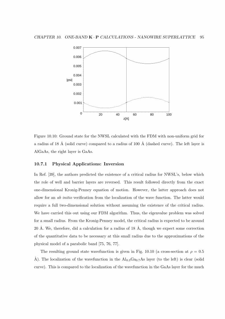
CHAPTER 10. ONE-BAND K · P CALCULATIONS - NANOWIRE SUPERLATTICE 95
0
0.001
0.002
0.003
0.004
0.005
0.006
0.007
|psi|
20 40 60 80 100z[A]
Figure 10.10: Ground state for the NWSL calculated with the FDM with non-uniform grid for
a radius of 18 A (solid curve) compared to a radius of 100 A (dashed curve). The left layer is
AlGaAs, the right layer is GaAs.
10.7.1 Physical Applications: Inversion
In Ref. [39], the authors predicted the existence of a critical radius for NWSL’s, below which
the role of well and barrier layers are reversed. This result followed directly from the exact
one-dimensional Kronig-Penney equation of motion. However, the latter approach does not
allow for an ab initio verification from the localization of the wave function. The latter would
require a full two-dimensional solution without assuming the existence of the critical radius.
We have carried this out using our FDM algorithm. Thus, the eigenvalue problem was solved
for a small radius. From the Kronig-Penney model, the critical radius is expected to be around
20 A. We, therefore, did a calculation for a radius of 18 A, though we expect some correction
of the quantitative data to be necessary at this small radius due to the approximations of the
physical model of a parabolic band [75, 76, 77].
The resulting ground state wavefunction is given in Fig. 10.10 (a cross-section at ρ = 0.5
A). The localization of the wavefunction in the Al0.3Ga0.7As layer (to the left) is clear (solid
curve). This is compared to the localization of the wavefunction in the GaAs layer for the much
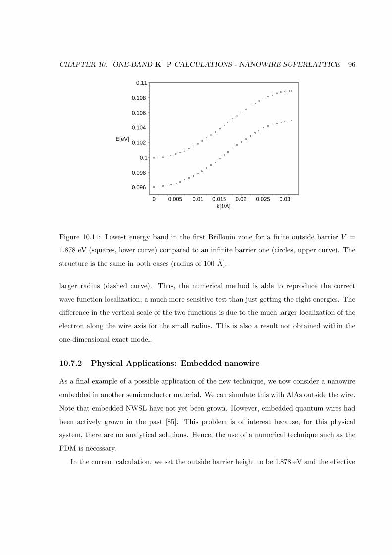
CHAPTER 10. ONE-BAND K · P CALCULATIONS - NANOWIRE SUPERLATTICE 96
0.096
0.098
0.1
0.102
0.104
0.106
0.108
0.11
E[eV]
0 0.005 0.01 0.015 0.02 0.025 0.03k[1/A]
Figure 10.11: Lowest energy band in the first Brillouin zone for a finite outside barrier V =
1.878 eV (squares, lower curve) compared to an infinite barrier one (circles, upper curve). The
structure is the same in both cases (radius of 100 A).
larger radius (dashed curve). Thus, the numerical method is able to reproduce the correct
wave function localization, a much more sensitive test than just getting the right energies. The
difference in the vertical scale of the two functions is due to the much larger localization of the
electron along the wire axis for the small radius. This is also a result not obtained within the
one-dimensional exact model.
10.7.2 Physical Applications: Embedded nanowire
As a final example of a possible application of the new technique, we now consider a nanowire
embedded in another semiconductor material. We can simulate this with AlAs outside the wire.
Note that embedded NWSL have not yet been grown. However, embedded quantum wires had
been actively grown in the past [85]. This problem is of interest because, for this physical
system, there are no analytical solutions. Hence, the use of a numerical technique such as the
FDM is necessary.
In the current calculation, we set the outside barrier height to be 1.878 eV and the effective
CHAPTER 10. ONE-BAND K · P CALCULATIONS - NANOWIRE SUPERLATTICE 97
mass to be 0.1 mo (pure AlAs). The grid in the z direction is the same as before for the infinite
barrier problem. In the radial direction, we now have a dimension of 100 A for the NWSL
(i.e. same radius of 100 A as before), and a width of 310 A for the AlAs layer. The grid in
the radial direction is 10 A at 1 A grid step, 100 A at 2 A, and 200 A at 4 A. Note that it
is not necessary to have too many points in the outside barrier since the wavefunction decays
exponentially there. In Fig. 10.11, we give the resulting energy band (lower curve) compared to
the infinite barrier result obtained earlier (upper curve). As expected, it is lower than with an
infinite barrier outside due to the reduced quantum confinement. For this particular structure,
the band is more or less uniformly lower by about 4 %. We are, therefore, in a position to
calculate the energies and wavefunctions of any NWSL, free standing or embedded, within the
one-band model.
10.8 Conclusions
The theory of the finite difference method in cylindrical polar coordinates and with periodic
boundary conditions (together with a non-uniform grid and a position-dependent mass) is
given in detail. In particular, the implementation of the boundary condition on the cylinder
axis is clarified. Applications to finite-length and infinite-length structures show that, for
a finite NWSL with barrier layers at both ends, only about six unit cells are necessary in
approximating the energy bands of a periodic system. However, the use of the Bloch theorem
speeds up the solution of the latter problem and reduces the memory requirements. Verification
of our two-dimensional computational model was achieved by comparing with one-dimensional
exact results. We then used the model to obtain a numerical proof of the possible existence of
inverted states without any a priori assumptions. New results were also obtained for the case
of an embedded nanowire for which there are no exact solutions.
Chapter 11
Eight-Band k · p Calculations - ZB
Quantum Well
11.1 Introduction
The simplest heterostructure to which we can apply the 8-band Hamiltonian is the quantum
well (QW). The calculation of intervalence subband optical transitions in quantum wells goes
back to a paper by Chang and James (CJ) in 1989 [40]. It established that these transitions
can have both TE and TM polarizations. The calculations were done using the four-band
Luttinger-Kohn (LK) Hamiltonian with infinite-barrier quantum-well states. Szmulowicz [29]
generalized the CJ equation to allow for position-dependent k · p parameters.
In this chapter we present an envelope-function-representation derivation and calculations of
the band structure and the momentum matrix elements between valence subbands in [001] quan-
tum wells using the Luttinger-Kohn-Kane and the Burt-Foreman Hamiltonians. We show how
to apply the finite difference method to solve the multi-band k · p equation for GaAs/Al0.3Ga0.7As
and GaAs/AlAs quantum wells. Then we use the eigenfunctions to calculate momentum ma-
trix elements, as described in Chapter 5. Both the Burt-Foreman and the Luttinger-Kohn
Hamiltonians are used, and differences between the two methods are pointed out.
98
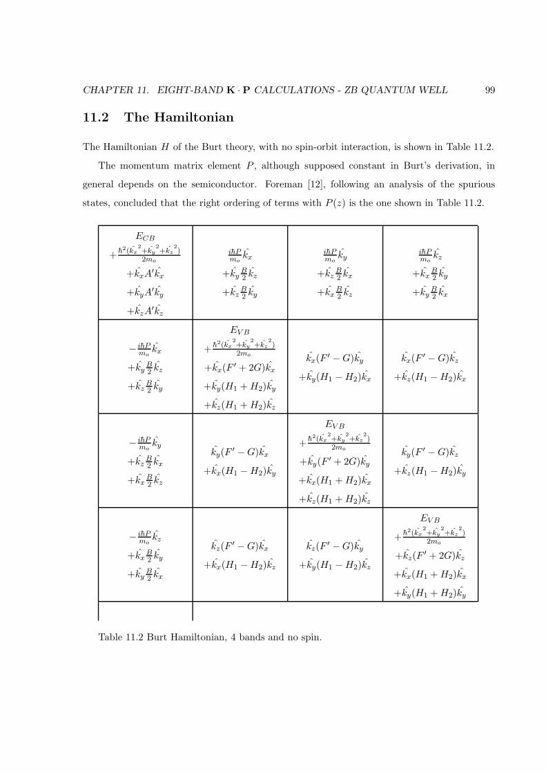
CHAPTER 11. EIGHT-BAND K · P CALCULATIONS - ZB QUANTUM WELL 99
11.2 The Hamiltonian
The Hamiltonian H of the Burt theory, with no spin-orbit interaction, is shown in Table 11.2.
The momentum matrix element P , although supposed constant in Burt’s derivation, in
general depends on the semiconductor. Foreman [12], following an analysis of the spurious
states, concluded that the right ordering of terms with P (z) is the one shown in Table 11.2.
ECB
+h2(kx
2+ky
2+kz
2)
2mo
+kxA′kx
+kyA′ky
+kzA′kz
ihPmo
kx
+kyB2 kz
+kzB2 ky
ihPmo
ky
+kzB2 kx
+kxB2 kz
ihPmo
kz
+kxB2 ky
+kyB2 kx
− ihPmo
kx
+kyB2 kz
+kzB2 ky
EV B
+ h2(kx2+ky
2+kz
2)
2mo
+kx(F ′ + 2G)kx
+ky(H1 +H2)ky
+kz(H1 +H2)kz
kx(F ′ −G)ky
+ky(H1 −H2)kx
kx(F ′ −G)kz
+kz(H1 −H2)kx
− ihPmo
ky
+kzB2 kx
+kxB2 kz
ky(F′ −G)kx
+kx(H1 −H2)ky
EV B
+h2(kx
2+ky
2+kz
2)
2mo
+ky(F′ + 2G)ky
+kx(H1 +H2)kx
+kz(H1 +H2)kz
ky(F′ −G)kz
+kz(H1 −H2)ky
− ihPmo
kz
+kxB2 ky
+kyB2 kx
kz(F′ −G)kx
+kx(H1 −H2)kz
kz(F′ −G)ky
+ky(H1 −H2)kz
EV B
+ h2(kx2+ky
2+kz
2)
2mo
+kz(F′ + 2G)kz
+kx(H1 +H2)kx
+ky(H1 +H2)ky
Table 11.2 Burt Hamiltonian, 4 bands and no spin.
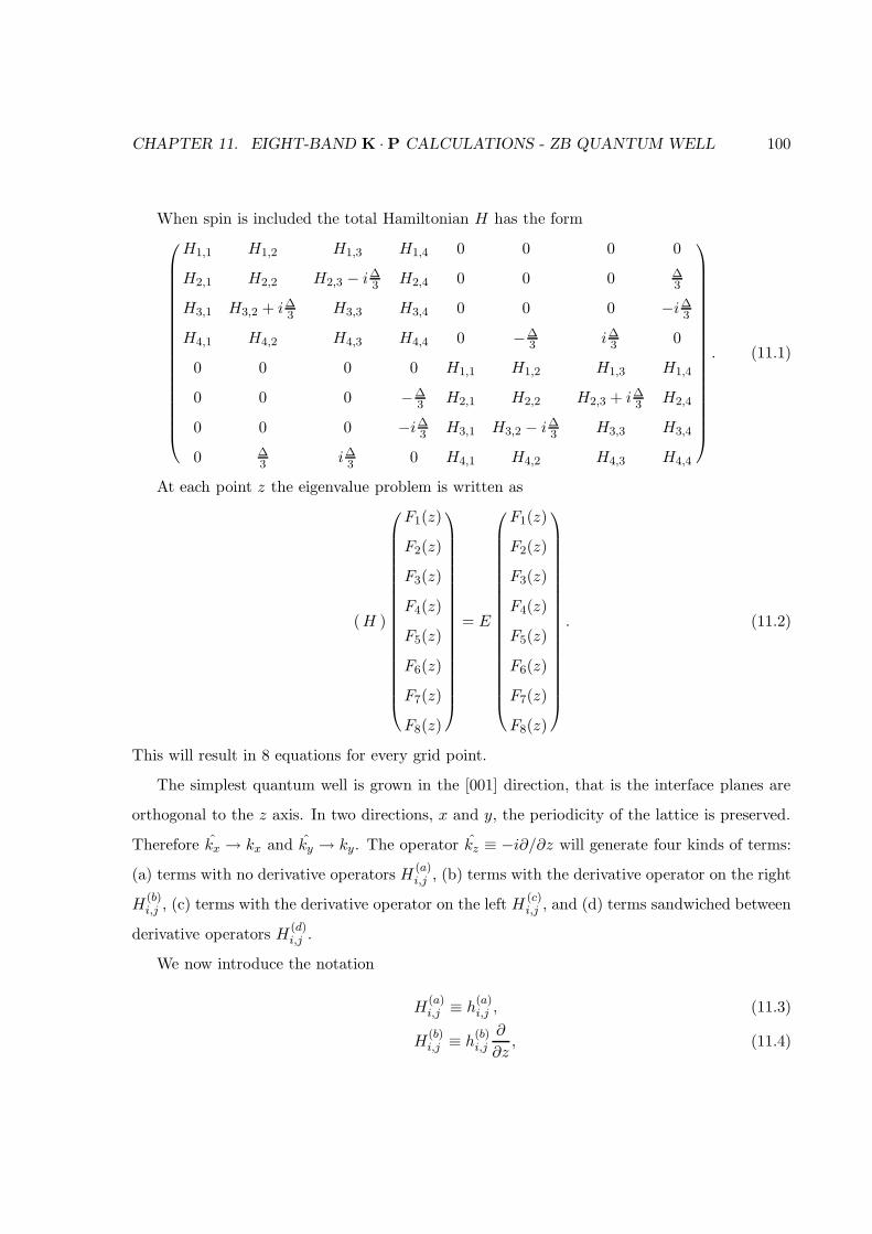
CHAPTER 11. EIGHT-BAND K · P CALCULATIONS - ZB QUANTUM WELL 100
When spin is included the total Hamiltonian H has the form
H1,1 H1,2 H1,3 H1,4 0 0 0 0
H2,1 H2,2 H2,3 − i∆3 H2,4 0 0 0 ∆3
H3,1 H3,2 + i∆3 H3,3 H3,4 0 0 0 −i∆3H4,1 H4,2 H4,3 H4,4 0 −∆
3 i∆3 0
0 0 0 0 H1,1 H1,2 H1,3 H1,4
0 0 0 −∆3 H2,1 H2,2 H2,3 + i∆3 H2,4
0 0 0 −i∆3 H3,1 H3,2 − i∆3 H3,3 H3,4
0 ∆3 i∆3 0 H4,1 H4,2 H4,3 H4,4
. (11.1)
At each point z the eigenvalue problem is written as
(H )
F1(z)
F2(z)
F3(z)
F4(z)
F5(z)
F6(z)
F7(z)
F8(z)
= E
F1(z)
F2(z)
F3(z)
F4(z)
F5(z)
F6(z)
F7(z)
F8(z)
. (11.2)
This will result in 8 equations for every grid point.
The simplest quantum well is grown in the [001] direction, that is the interface planes are
orthogonal to the z axis. In two directions, x and y, the periodicity of the lattice is preserved.
Therefore kx → kx and ky → ky. The operator kz ≡ −i∂/∂z will generate four kinds of terms:
(a) terms with no derivative operators H(a)i,j , (b) terms with the derivative operator on the right
H(b)i,j , (c) terms with the derivative operator on the left H
(c)i,j , and (d) terms sandwiched between
derivative operators H(d)i,j .
We now introduce the notation
H(a)i,j ≡ h
(a)i,j , (11.3)
H(b)i,j ≡ h
(b)i,j
∂
∂z, (11.4)
CHAPTER 11. EIGHT-BAND K · P CALCULATIONS - ZB QUANTUM WELL 101
H(c)i,j ≡ ∂
∂zh
(c)i,j , (11.5)
H(d)i,j ≡ ∂
∂zh
(d)i,j
∂
∂z. (11.6)
The Hamiltonian elements of type (a) are
h(a)1,1 = ECB +
h2(k2x + k2
y)
2mo+A′(k2
x + k2y), (11.7)
h(a)1,2 =
ihP
mokx, (11.8)
h(a)1,3 =
ihP
moky, (11.9)
h(a)1,4 = Bkxky, (11.10)
h(a)2,1 = − ihP
mokx, (11.11)
h(a)2,2 = EV B +
h2(k2x + k2
y)
2mo+ (F ′ + 2G)k2
x + (H1 +H2)k2y , (11.12)
h(a)2,3 = (F ′ −G)kxky + (H1 −H2)kxky, (11.13)
h(a)3,1 = − ihP
moky, (11.14)
h(a)3,2 = (F ′ −G)kxky + (H1 −H2)kxky, (11.15)
h(a)3,3 = EV B +
h2(k2x + k2
y)
2mo+ (F ′ + 2G)k2
y + (H1 +H2)k2x, (11.16)
h(a)4,1 = Bkxky, (11.17)
h(a)4,4 = EV B +
h2(k2x + k2
y)
2mo+ (H1 +H2)k
2x + (H1 +H2)k
2y . (11.18)
The Hamiltonian elements of type (b) are
h(b)1,2 = −iky
B
2, (11.19)
h(b)1,3 = −ikx
B
2, (11.20)
h(b)1,4 =
hP
mo, (11.21)
h(b)2,1 = −iky
B
2, (11.22)
h(b)2,4 = −ikx(F ′ −G), (11.23)
h(b)3,1 = −ikx
B
2, (11.24)
h(b)3,4 = −iky(F
′ −G), (11.25)
CHAPTER 11. EIGHT-BAND K · P CALCULATIONS - ZB QUANTUM WELL 102
h(b)4,1 = − hP
mo, (11.26)
h(b)4,2 = −ikx(H1 −H2), (11.27)
h(b)4,3 = −iky(H1 −H2). (11.28)
The Hamiltonian elements of type (c) are
h(c)1,2 = −iB
2ky, (11.29)
h(c)1,3 = −iB
2kx, (11.30)
h(c)2,1 = −iB
2ky, (11.31)
h(c)2,4 = −i(H1 −H2)kx, (11.32)
h(c)3,1 = −iB
2kx, (11.33)
h(c)3,4 = −i(H1 −H2)ky, (11.34)
h(c)4,2 = −i(F ′ −G)kx, (11.35)
h(c)4,3 = −i(F ′ −G)ky . (11.36)
The Hamiltonian elements of type (d) are
h(d)1,1 = −(
h2
2mo+A′), (11.37)
h(d)2,2 = −(
h2
2mo+H1 +H2), (11.38)
h(d)3,3 = −(
h2
2mo+H1 +H2), (11.39)
h(d)4,4 = −(
h2
2mo+ F ′ + 2G). (11.40)
11.3 The Finite Difference Method
Let n label grid points along the z direction. With the notation Fj,n ≡ Fj(zn), hi,j,n ≡ hi,j(zn),
the derivatives are calculated with a central difference scheme on the non-uniform grid as
∂Fj,n
∂z= Fj,n−1An + Fj,nBn + Fj,n+1Cn, (11.41)
CHAPTER 11. EIGHT-BAND K · P CALCULATIONS - ZB QUANTUM WELL 103
where
An ≡ −∆zn∆zn−1(∆zn−1 + ∆zn)
, (11.42)
Bn ≡ ∆zn − ∆zn−1
∆zn−1∆zn, (11.43)
Cn ≡ ∆zn−1
∆zn(∆zn−1 + ∆zn), (11.44)
and ∆zn ≡ zn+1 − zn.
The terms sandwiched between derivatives are expanded as
∂
∂z
(h
(d)i,j,n
∂Fj,n
∂z
)
= h(d)i,j,n−1/2
∂Fj,n−1/2
∂z2An + h
(d)i,j,n
∂Fj,n
∂z2Bn + h
(d)i,j,n+1/2
∂Fj,n+1/2
∂z2Cn
=h
(d)i,j,n−1 + h
(d)i,j,n
2
Fj,n − Fj,n−1
∆zn−12An + h
(d)i,j,n
Fj,n+1 − Fj,n−1
∆zn−1 + ∆zn2Bn (11.45)
+h
(d)i,j,n+1 + h
(d)i,j,n
2
Fj,n+1 − Fj,n
∆zn2Cn.
In conclusion, four contributions appear in the eigenvalue problem:
h(a)i,j,nFj,n = h
(a)i,j,nFj,n, (11.46)
h(b)i,j,n
∂
∂zFj,n = Fj,n−1Anh
(b)i,j,n + Fj,nBnh
(b)i,j,n + Fj,n+1Cnh
(b)i,j,n, (11.47)
∂
∂zh
(c)i,j,nFj,n = Fj,n−1h
(c)i,j,n−1An + Fj,nh
(c)i,j,nBn + Fj,n+1h
(c)i,j,n+1Cn, (11.48)
∂
∂zh
(d)i,j,n
∂
∂zFj,n = Fj,n−1
−
h(d)i,j,n−1 + h
(d)i,j,n
∆zn−1An −
h(d)i,j,n
∆zn−1 + ∆zn2Bn
+Fj,n
h
(d)i,j,n−1 + h
(d)i,j,n
∆zn−1An −
h(d)i,j,n+1 + h
(d)i,j,n
∆znCn
+Fj,n+1
h
(d)i,j,n
∆zn−1 + ∆zn2Bn +
h(d)i,j,n+1 + h
(d)i,j,n
∆znCn
. (11.49)
When spin is included we have additional terms hi+4,j+4,n = hi,j,n. The spin-orbit Hamil-
tonian will give an extra contribution of type (a).
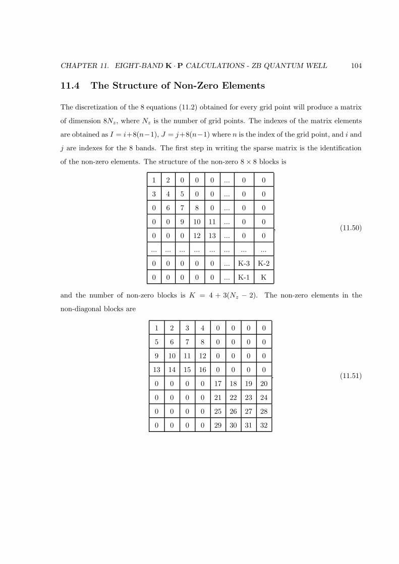
CHAPTER 11. EIGHT-BAND K · P CALCULATIONS - ZB QUANTUM WELL 104
11.4 The Structure of Non-Zero Elements
The discretization of the 8 equations (11.2) obtained for every grid point will produce a matrix
of dimension 8Nz, where Nz is the number of grid points. The indexes of the matrix elements
are obtained as I = i+8(n−1), J = j+8(n−1) where n is the index of the grid point, and i and
j are indexes for the 8 bands. The first step in writing the sparse matrix is the identification
of the non-zero elements. The structure of the non-zero 8 × 8 blocks is
1 2 0 0 0 ... 0 0
3 4 5 0 0 ... 0 0
0 6 7 8 0 ... 0 0
0 0 9 10 11 ... 0 0
0 0 0 12 13 ... 0 0
... ... ... ... ... ... ... ...
0 0 0 0 0 ... K-3 K-2
0 0 0 0 0 ... K-1 K
, (11.50)
and the number of non-zero blocks is K = 4 + 3(Nz − 2). The non-zero elements in the
non-diagonal blocks are
1 2 3 4 0 0 0 0
5 6 7 8 0 0 0 0
9 10 11 12 0 0 0 0
13 14 15 16 0 0 0 0
0 0 0 0 17 18 19 20
0 0 0 0 21 22 23 24
0 0 0 0 25 26 27 28
0 0 0 0 29 30 31 32
. (11.51)
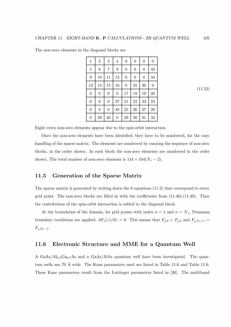
CHAPTER 11. EIGHT-BAND K · P CALCULATIONS - ZB QUANTUM WELL 105
The non-zero elements in the diagonal blocks are
1 2 3 4 0 0 0 0
5 6 7 8 0 0 0 33
9 10 11 12 0 0 0 34
13 14 15 16 0 35 36 0
0 0 0 0 17 18 19 20
0 0 0 37 21 22 23 24
0 0 0 38 25 26 27 28
0 39 40 0 29 30 31 32
. (11.52)
Eight extra non-zero elements appear due to the spin-orbit interaction.
Once the non-zero elements have been identified, they have to be numbered, for the easy
handling of the sparse matrix. The elements are numbered by running the sequence of non-zero
blocks, in the order shown. In each block the non-zero elements are numbered in the order
shown. The total number of non-zero elements is 144 + 104(Nz − 2).
11.5 Generation of the Sparse Matrix
The sparse matrix is generated by writing down the 8 equations (11.2) that correspond to every
grid point. The non-zero blocks are filled in with the coefficients from (11.46)-(11.49). Then
the contribution of the spin-orbit interaction is added to the diagonal block.
At the boundaries of the domain, for grid points with index n = 1 and n = Nz, Neumann
boundary conditions are applied: ∂Fj(z)/∂z = 0. This means that Fj,0 = Fj,2 and Fj,Nz+1 =
Fj,Nz−1.
11.6 Electronic Structure and MME for a Quantum Well
A GaAs/Al0.3Ga0.7As and a GaAs/AlAs quantum well have been investigated. The quan-
tum wells are 70 A wide. The Kane parameters used are listed in Table 11.6 and Table 11.6.
These Kane parameters result from the Luttinger parameters listed in [30]. The multiband
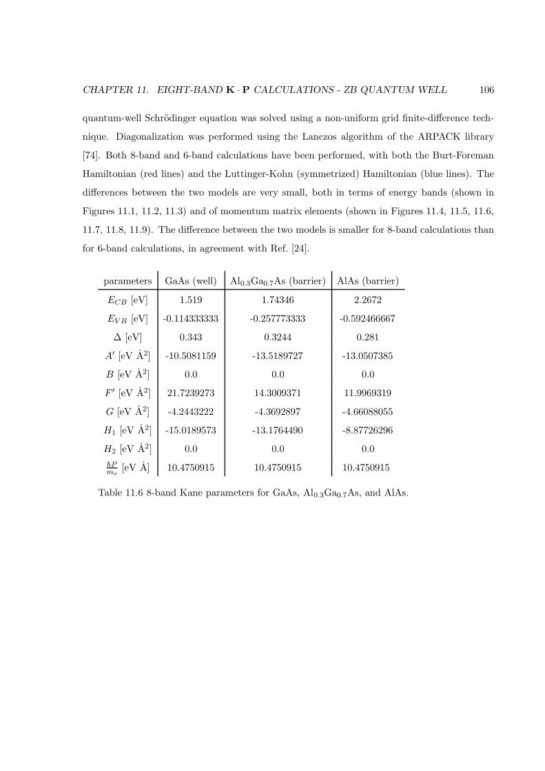
CHAPTER 11. EIGHT-BAND K · P CALCULATIONS - ZB QUANTUM WELL 106
quantum-well Schrodinger equation was solved using a non-uniform grid finite-difference tech-
nique. Diagonalization was performed using the Lanczos algorithm of the ARPACK library
[74]. Both 8-band and 6-band calculations have been performed, with both the Burt-Foreman
Hamiltonian (red lines) and the Luttinger-Kohn (symmetrized) Hamiltonian (blue lines). The
differences between the two models are very small, both in terms of energy bands (shown in
Figures 11.1, 11.2, 11.3) and of momentum matrix elements (shown in Figures 11.4, 11.5, 11.6,
11.7, 11.8, 11.9). The difference between the two models is smaller for 8-band calculations than
for 6-band calculations, in agreement with Ref. [24].
parameters GaAs (well) Al0.3Ga0.7As (barrier) AlAs (barrier)
ECB [eV] 1.519 1.74346 2.2672
EV B [eV] -0.114333333 -0.257773333 -0.592466667
∆ [eV] 0.343 0.3244 0.281
A′ [eV A2] -10.5081159 -13.5189727 -13.0507385
B [eV A2] 0.0 0.0 0.0
F ′ [eV A2] 21.7239273 14.3009371 11.9969319
G [eV A2] -4.2443222 -4.3692897 -4.66088055
H1 [eV A2] -15.0189573 -13.1764490 -8.87726296
H2 [eV A2] 0.0 0.0 0.0
hPmo
[eV A] 10.4750915 10.4750915 10.4750915
Table 11.6 8-band Kane parameters for GaAs, Al0.3Ga0.7As, and AlAs.
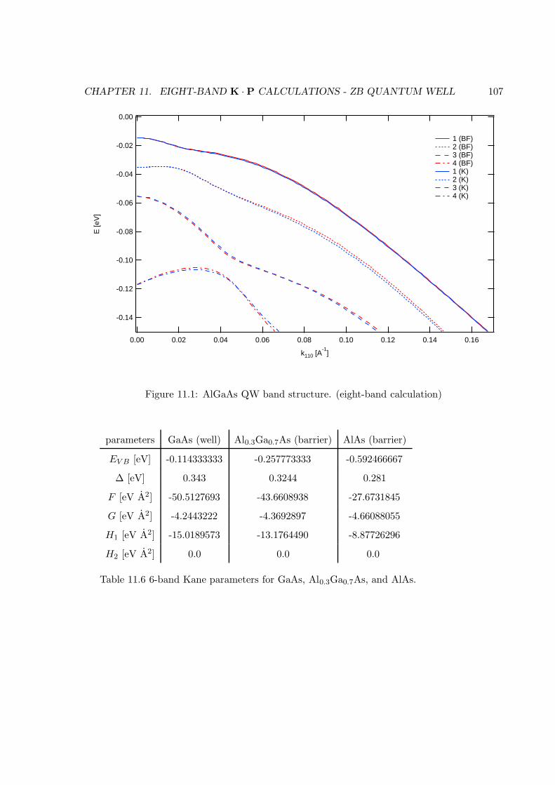
CHAPTER 11. EIGHT-BAND K · P CALCULATIONS - ZB QUANTUM WELL 107
-0.14
-0.12
-0.10
-0.08
-0.06
-0.04
-0.02
0.00
E [e
V]
0.160.140.120.100.080.060.040.020.00
k110 [A-1
]
1 (BF) 2 (BF) 3 (BF) 4 (BF) 1 (K) 2 (K) 3 (K) 4 (K)
Figure 11.1: AlGaAs QW band structure. (eight-band calculation)
parameters GaAs (well) Al0.3Ga0.7As (barrier) AlAs (barrier)
EV B [eV] -0.114333333 -0.257773333 -0.592466667
∆ [eV] 0.343 0.3244 0.281
F [eV A2] -50.5127693 -43.6608938 -27.6731845
G [eV A2] -4.2443222 -4.3692897 -4.66088055
H1 [eV A2] -15.0189573 -13.1764490 -8.87726296
H2 [eV A2] 0.0 0.0 0.0
Table 11.6 6-band Kane parameters for GaAs, Al0.3Ga0.7As, and AlAs.
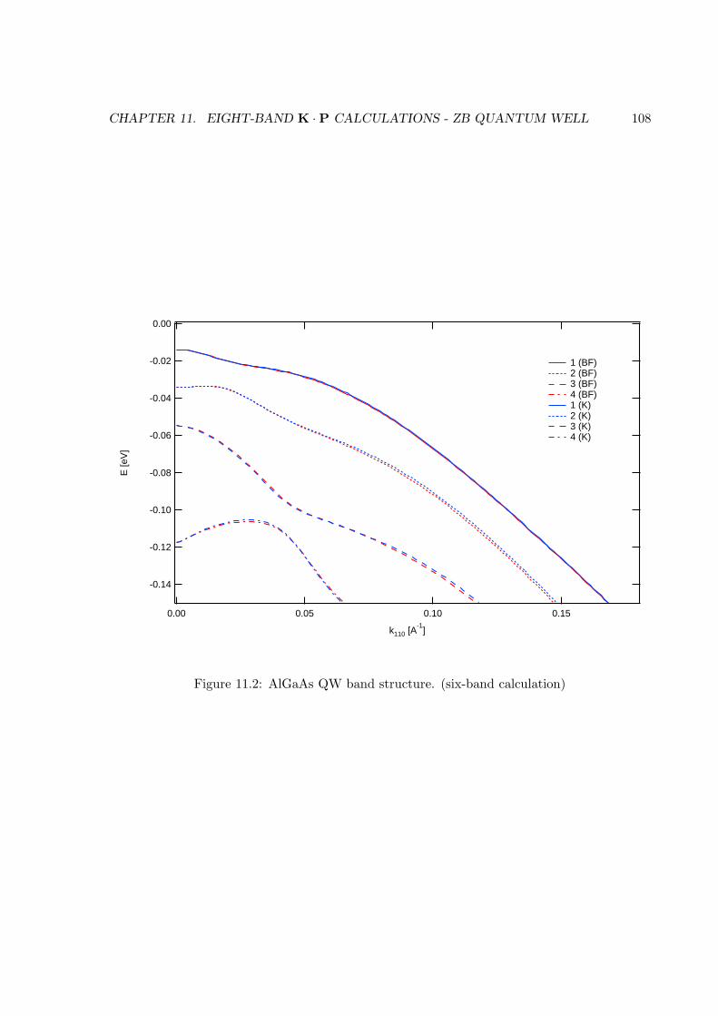
CHAPTER 11. EIGHT-BAND K · P CALCULATIONS - ZB QUANTUM WELL 108
-0.14
-0.12
-0.10
-0.08
-0.06
-0.04
-0.02
0.00
E [e
V]
0.150.100.050.00
k110 [A-1
]
1 (BF) 2 (BF) 3 (BF) 4 (BF) 1 (K) 2 (K) 3 (K) 4 (K)
Figure 11.2: AlGaAs QW band structure. (six-band calculation)
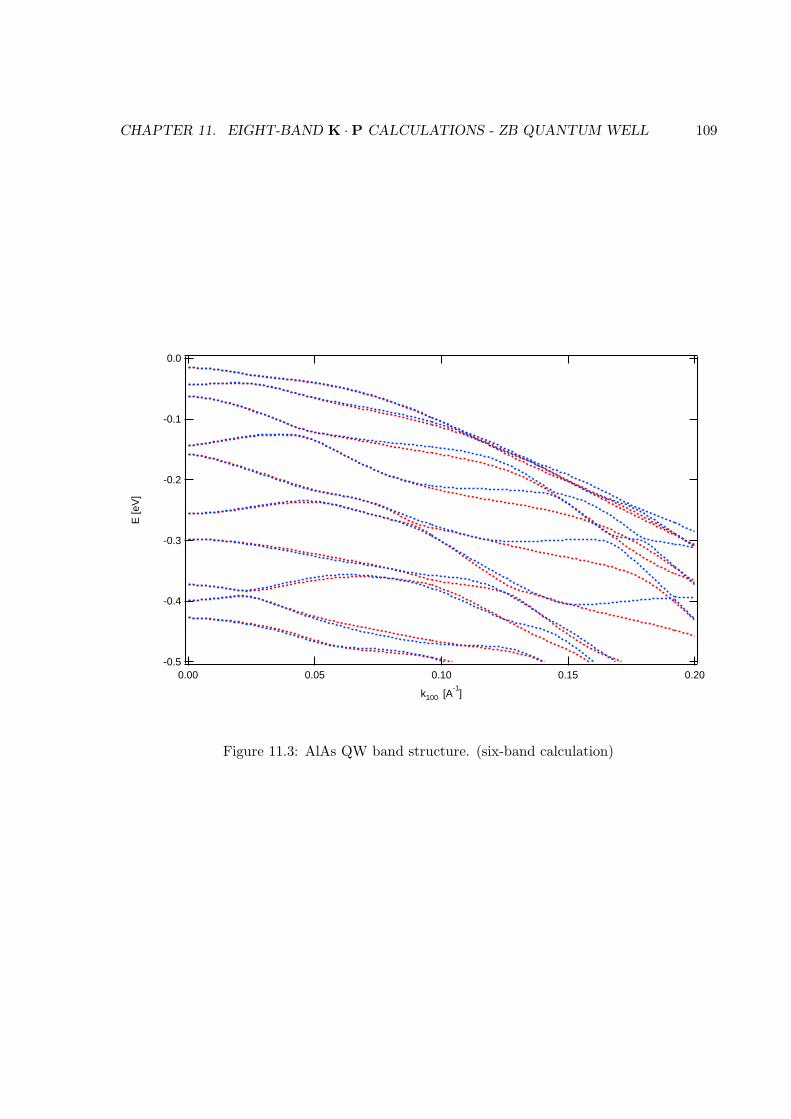
CHAPTER 11. EIGHT-BAND K · P CALCULATIONS - ZB QUANTUM WELL 109
-0.5
-0.4
-0.3
-0.2
-0.1
0.0
E [e
V]
0.200.150.100.050.00
k100 [A-1
]
Figure 11.3: AlAs QW band structure. (six-band calculation)
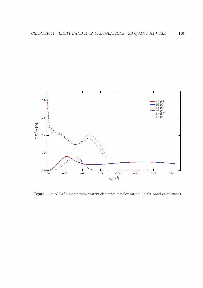
CHAPTER 11. EIGHT-BAND K · P CALCULATIONS - ZB QUANTUM WELL 110
0.8
0.6
0.4
0.2
0.0
2 |P
x|2 /m
[eV
]
0.140.120.100.080.060.040.020.00
k110 [A-1
]
1-2 (BF)1-2 (K)1-3 (BF)1-3 (K)1-4 (BF)1-4 (K)
Figure 11.4: AlGaAs momentum matrix elements: x polarization. (eight-band calculation)
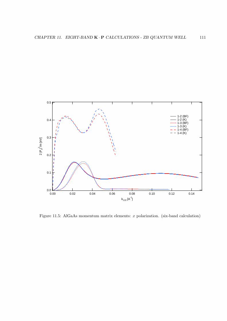
CHAPTER 11. EIGHT-BAND K · P CALCULATIONS - ZB QUANTUM WELL 111
0.5
0.4
0.3
0.2
0.1
0.0
2 |P
x|2 /m
[eV
]
0.140.120.100.080.060.040.020.00
k110 [A-1
]
1-2 (BF) 1-2 (K) 1-3 (BF) 1-3 (K) 1-4 (BF) 1-4 (K)
Figure 11.5: AlGaAs momentum matrix elements: x polarization. (six-band calculation)
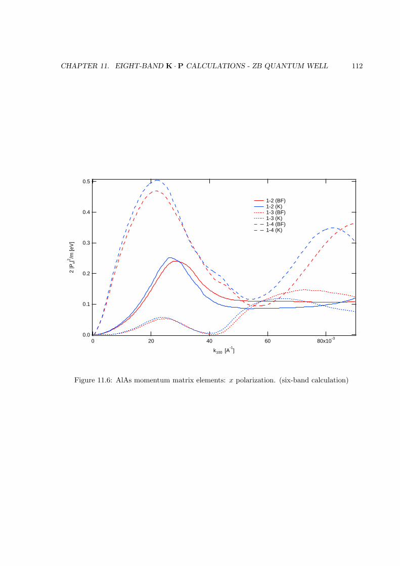
CHAPTER 11. EIGHT-BAND K · P CALCULATIONS - ZB QUANTUM WELL 112
0.5
0.4
0.3
0.2
0.1
0.0
2 |P
x|2 /m
[eV
]
80x10-3
6040200
k100 [A-1
]
1-2 (BF) 1-2 (K) 1-3 (BF) 1-3 (K) 1-4 (BF) 1-4 (K)
Figure 11.6: AlAs momentum matrix elements: x polarization. (six-band calculation)
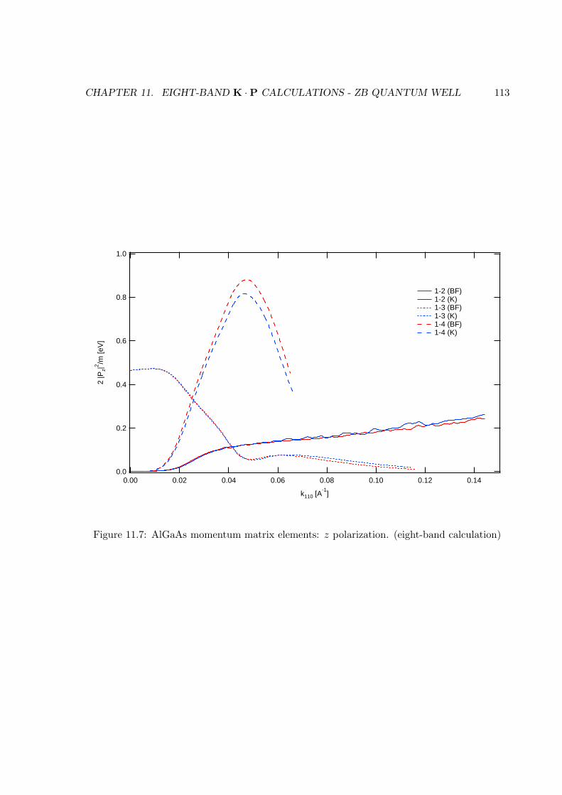
CHAPTER 11. EIGHT-BAND K · P CALCULATIONS - ZB QUANTUM WELL 113
1.0
0.8
0.6
0.4
0.2
0.0
2 |P
z|2 /m
[eV
]
0.140.120.100.080.060.040.020.00
k110 [A-1
]
1-2 (BF) 1-2 (K) 1-3 (BF) 1-3 (K) 1-4 (BF) 1-4 (K)
Figure 11.7: AlGaAs momentum matrix elements: z polarization. (eight-band calculation)
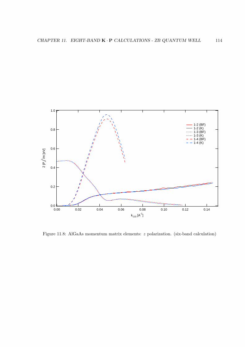
CHAPTER 11. EIGHT-BAND K · P CALCULATIONS - ZB QUANTUM WELL 114
1.0
0.8
0.6
0.4
0.2
0.0
2 |P
z|2 /m
[eV
]
0.140.120.100.080.060.040.020.00
k110 [A-1
]
1-2 (BF) 1-2 (K) 1-3 (BF) 1-3 (K) 1-4 (BF) 1-4 (K)
Figure 11.8: AlGaAs momentum matrix elements: z polarization. (six-band calculation)
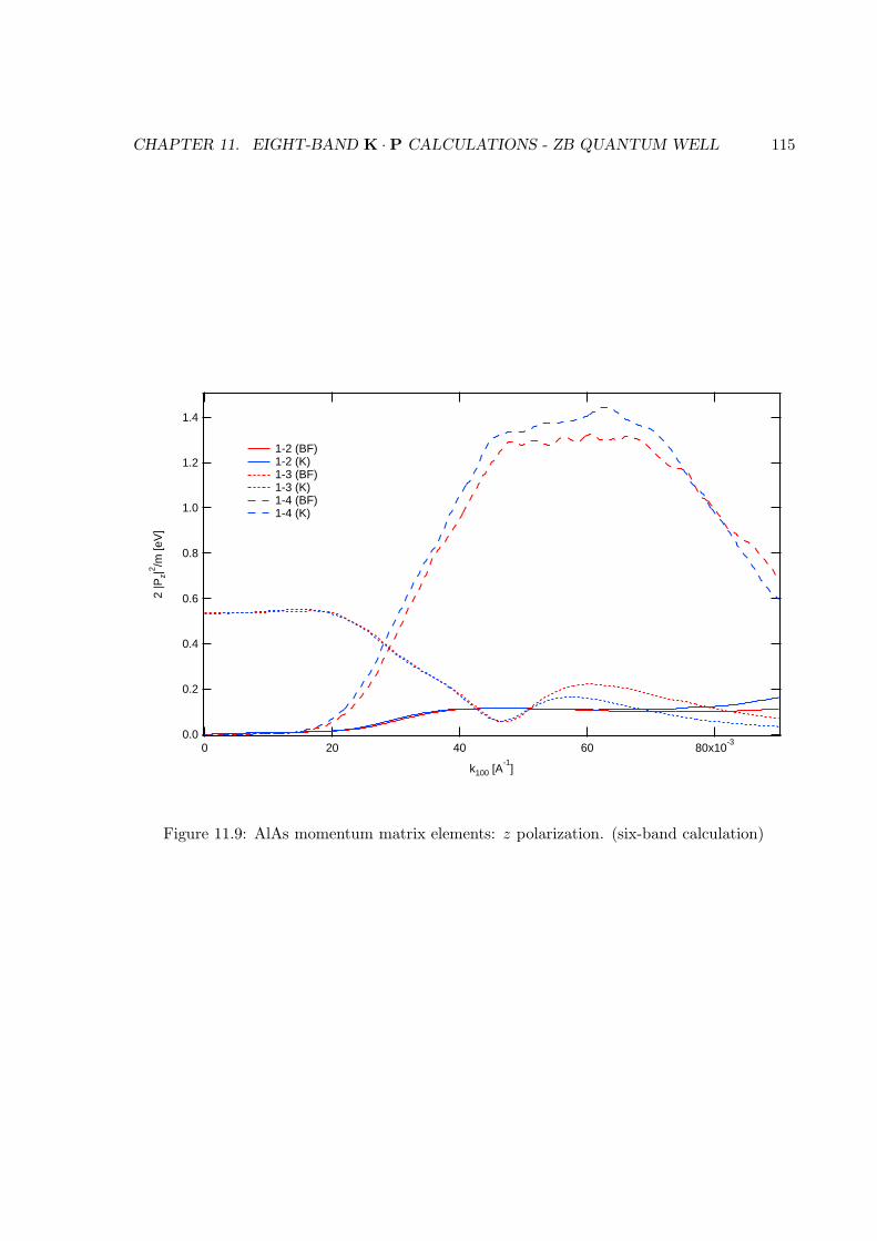
CHAPTER 11. EIGHT-BAND K · P CALCULATIONS - ZB QUANTUM WELL 115
1.4
1.2
1.0
0.8
0.6
0.4
0.2
0.0
2 |P
z|2 /m
[eV
]
80x10-3
6040200
k100 [A-1
]
1-2 (BF) 1-2 (K) 1-3 (BF) 1-3 (K) 1-4 (BF) 1-4 (K)
Figure 11.9: AlAs momentum matrix elements: z polarization. (six-band calculation)
Chapter 12
Six-Band k · p Calculations - WZ
Cylindrical Dot
12.1 Introduction
The III-V nitride semiconductors, with wurtzite (WZ) crystal structure, have received a great
deal of attention in recent years. In the 1950’s there were numerous optical studies of bulk
WZ semiconductors (see Ref. [41] for a recent review). However, the detailed band structure of
these materials was not studied until the discovery (in 1993) of blue light emission of WZ GaN
on sapphire [3]. Currently the interest in WZ materials has shifted to nanostructures such as
CdSe quantum rods [86, 87, 88], ZnS nanowires [89], ZnO nanorods [90] and nanowires [91],
AlN nanorods [92], and GaN nanowires [93]. On the theory side, the k · p theory of WZ bulk
materials was developed by Rashba and Pikus [94, 33] and later applied to heterostructures by
a number of authors [95, 31]. Mireles and Ulloa [25] have applied the theory to heterostructures
using the envelope function formalism of Burt [10] and Foreman [12]. As far as we are aware,
the model has only been applied to quantum wells [71] and pyramidal quantum dots [96]. In
1990, Sercel and Vahala (SV) presented a new formulation of the multiband envelope function
theory and applied it to spherical quantum dots and cylindrical quantum wires of zincblende
(ZB) materials [42, 43]. For ZB, the SV formulation was only possible provided the axial
approximation (γ2 = γ3) was made in the Hamiltonian. The theory, within the Luttinger-
116
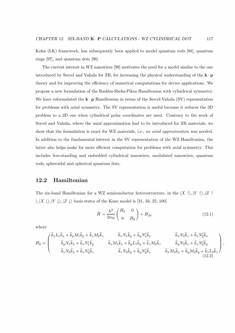
CHAPTER 12. SIX-BAND K ·P CALCULATIONS - WZ CYLINDRICAL DOT 117
Kohn (LK) framework, has subsequently been applied to model quantum rods [88], quantum
rings [97], and quantum dots [98].
The current interest in WZ nanowires [99] motivates the need for a model similar to the one
introduced by Sercel and Vahala for ZB, for increasing the physical understanding of the k · ptheory and for improving the efficiency of numerical computations for device applications. We
propose a new formulation of the Rashba-Sheka-Pikus Hamiltonian with cylindrical symmetry.
We have reformulated the k · p Hamiltonian in terms of the Sercel-Vahala (SV) representation
for problems with axial symmetry. The SV representation is useful because it reduces the 3D
problem to a 2D one when cylindrical polar coordinates are used. Contrary to the work of
Sercel and Vahala, where the axial approximation had to be introduced for ZB materials, we
show that the formulation is exact for WZ materials, i.e., no axial approximation was needed.
In addition to the fundamental interest in the SV representation of the WZ Hamiltonian, the
latter also helps make for more efficient computation for problems with axial symmetry. This
includes free-standing and embedded cylindrical nanowires, modulated nanowires, quantum
rods, spheroidal and spherical quantum dots.
12.2 Hamiltonian
The six-band Hamiltonian for a WZ semiconductor heterostructure, in the |X ↑〉, |Y ↑〉, |Z ↑〉, |X ↓〉, |Y ↓〉, |Z ↓〉 basis states of the Kane model is [31, 33, 25, 100]
H =h2
2m0
(Hk 0
0 Hk
)+H∆, (12.1)
where
Hk =
kxL1kx + kyM1ky + kzM2kz kxN1ky + kyN′1kx kxN2kz + kzN
′2kx
kyN1kx + kxN′1ky kxM1kx + kyL1ky + kzM2kz kyN2kz + kzN
′2ky
kzN2kx + kxN′2kz kzN2ky + kyN
′2kz kxM3kx + kyM3ky + kzL2kz
,
(12.2)
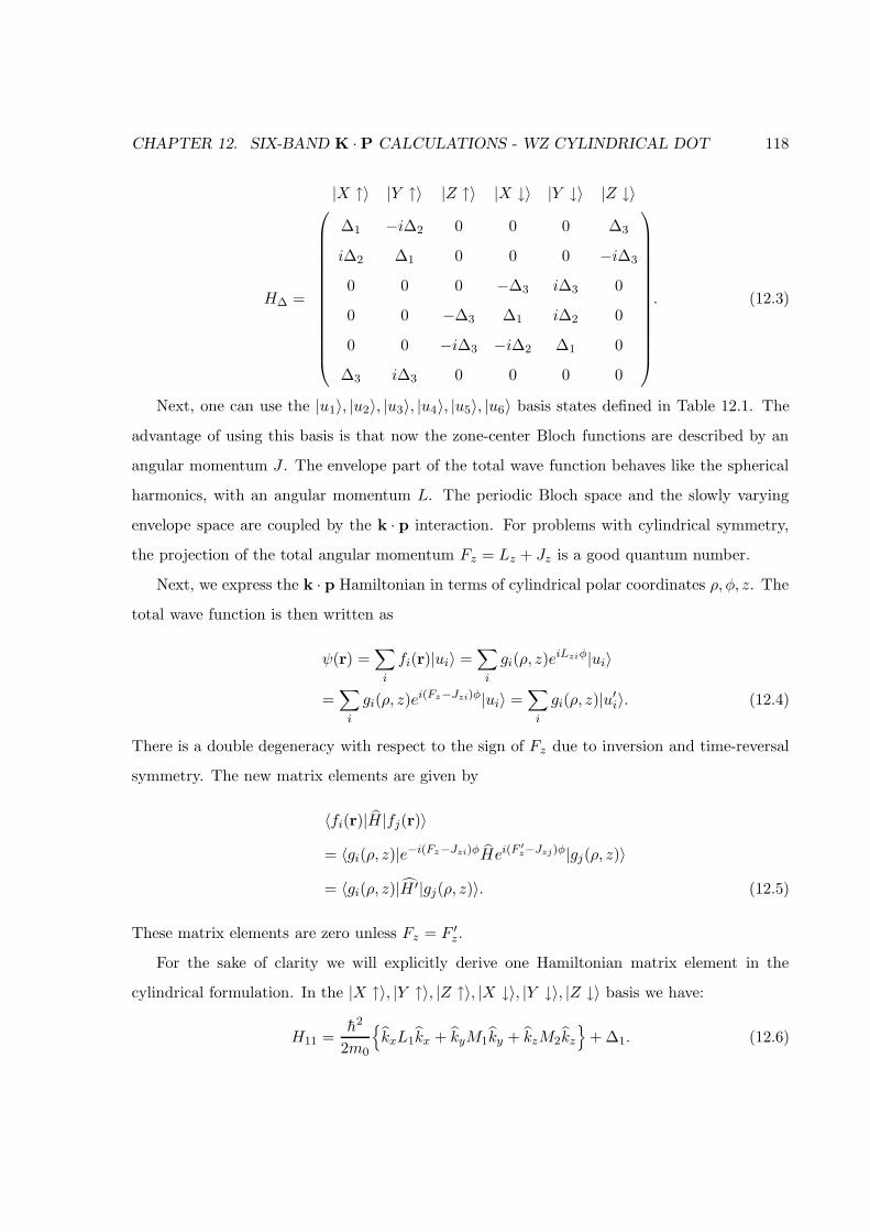
CHAPTER 12. SIX-BAND K ·P CALCULATIONS - WZ CYLINDRICAL DOT 118
H∆ =
|X ↑〉 |Y ↑〉 |Z ↑〉 |X ↓〉 |Y ↓〉 |Z ↓〉
∆1 −i∆2 0 0 0 ∆3
i∆2 ∆1 0 0 0 −i∆3
0 0 0 −∆3 i∆3 0
0 0 −∆3 ∆1 i∆2 0
0 0 −i∆3 −i∆2 ∆1 0
∆3 i∆3 0 0 0 0
. (12.3)
Next, one can use the |u1〉, |u2〉, |u3〉, |u4〉, |u5〉, |u6〉 basis states defined in Table 12.1. The
advantage of using this basis is that now the zone-center Bloch functions are described by an
angular momentum J . The envelope part of the total wave function behaves like the spherical
harmonics, with an angular momentum L. The periodic Bloch space and the slowly varying
envelope space are coupled by the k · p interaction. For problems with cylindrical symmetry,
the projection of the total angular momentum Fz = Lz + Jz is a good quantum number.
Next, we express the k · p Hamiltonian in terms of cylindrical polar coordinates ρ, φ, z. The
total wave function is then written as
ψ(r) =∑
i
fi(r)|ui〉 =∑
i
gi(ρ, z)eiLziφ|ui〉
=∑
i
gi(ρ, z)ei(Fz−Jzi)φ|ui〉 =
∑
i
gi(ρ, z)|u′i〉. (12.4)
There is a double degeneracy with respect to the sign of Fz due to inversion and time-reversal
symmetry. The new matrix elements are given by
〈fi(r)|H |fj(r)〉
= 〈gi(ρ, z)|e−i(Fz−Jzi)φHei(F′
z−Jzj)φ|gj(ρ, z)〉
= 〈gi(ρ, z)|H ′|gj(ρ, z)〉. (12.5)
These matrix elements are zero unless Fz = F ′z.
For the sake of clarity we will explicitly derive one Hamiltonian matrix element in the
cylindrical formulation. In the |X ↑〉, |Y ↑〉, |Z ↑〉, |X ↓〉, |Y ↓〉, |Z ↓〉 basis we have:
H11 =h2
2m0
kxL1kx + kyM1ky + kzM2kz
+ ∆1. (12.6)
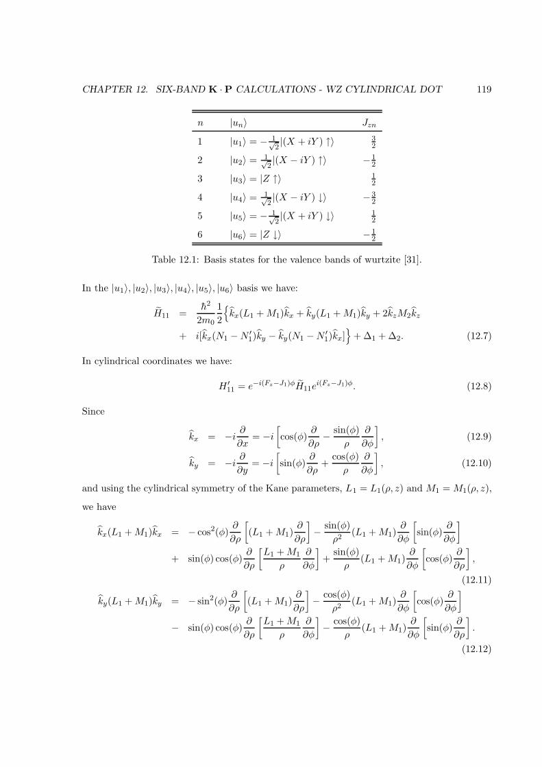
CHAPTER 12. SIX-BAND K ·P CALCULATIONS - WZ CYLINDRICAL DOT 119
n |un〉 Jzn
1 |u1〉 = − 1√2|(X + iY ) ↑〉 3
2
2 |u2〉 = 1√2|(X − iY ) ↑〉 − 1
2
3 |u3〉 = |Z ↑〉 12
4 |u4〉 = 1√2|(X − iY ) ↓〉 − 3
2
5 |u5〉 = − 1√2|(X + iY ) ↓〉 1
2
6 |u6〉 = |Z ↓〉 − 12
Table 12.1: Basis states for the valence bands of wurtzite [31].
In the |u1〉, |u2〉, |u3〉, |u4〉, |u5〉, |u6〉 basis we have:
H11 =h2
2m0
1
2
kx(L1 +M1)kx + ky(L1 +M1)ky + 2kzM2kz
+ i[kx(N1 −N ′1)ky − ky(N1 −N ′
1)kx]
+ ∆1 + ∆2. (12.7)
In cylindrical coordinates we have:
H ′11 = e−i(Fz−J1)φH11e
i(Fz−J1)φ. (12.8)
Since
kx = −i ∂∂x
= −i[cos(φ)
∂
∂ρ− sin(φ)
ρ
∂
∂φ
], (12.9)
ky = −i ∂∂y
= −i[sin(φ)
∂
∂ρ+
cos(φ)
ρ
∂
∂φ
], (12.10)
and using the cylindrical symmetry of the Kane parameters, L1 = L1(ρ, z) and M1 = M1(ρ, z),
we have
kx(L1 +M1)kx = − cos2(φ)∂
∂ρ
[(L1 +M1)
∂
∂ρ
]− sin(φ)
ρ2(L1 +M1)
∂
∂φ
[sin(φ)
∂
∂φ
]
+ sin(φ) cos(φ)∂
∂ρ
[L1 +M1
ρ
∂
∂φ
]+
sin(φ)
ρ(L1 +M1)
∂
∂φ
[cos(φ)
∂
∂ρ
],
(12.11)
ky(L1 +M1)ky = − sin2(φ)∂
∂ρ
[(L1 +M1)
∂
∂ρ
]− cos(φ)
ρ2(L1 +M1)
∂
∂φ
[cos(φ)
∂
∂φ
]
− sin(φ) cos(φ)∂
∂ρ
[L1 +M1
ρ
∂
∂φ
]− cos(φ)
ρ(L1 +M1)
∂
∂φ
[sin(φ)
∂
∂ρ
].
(12.12)
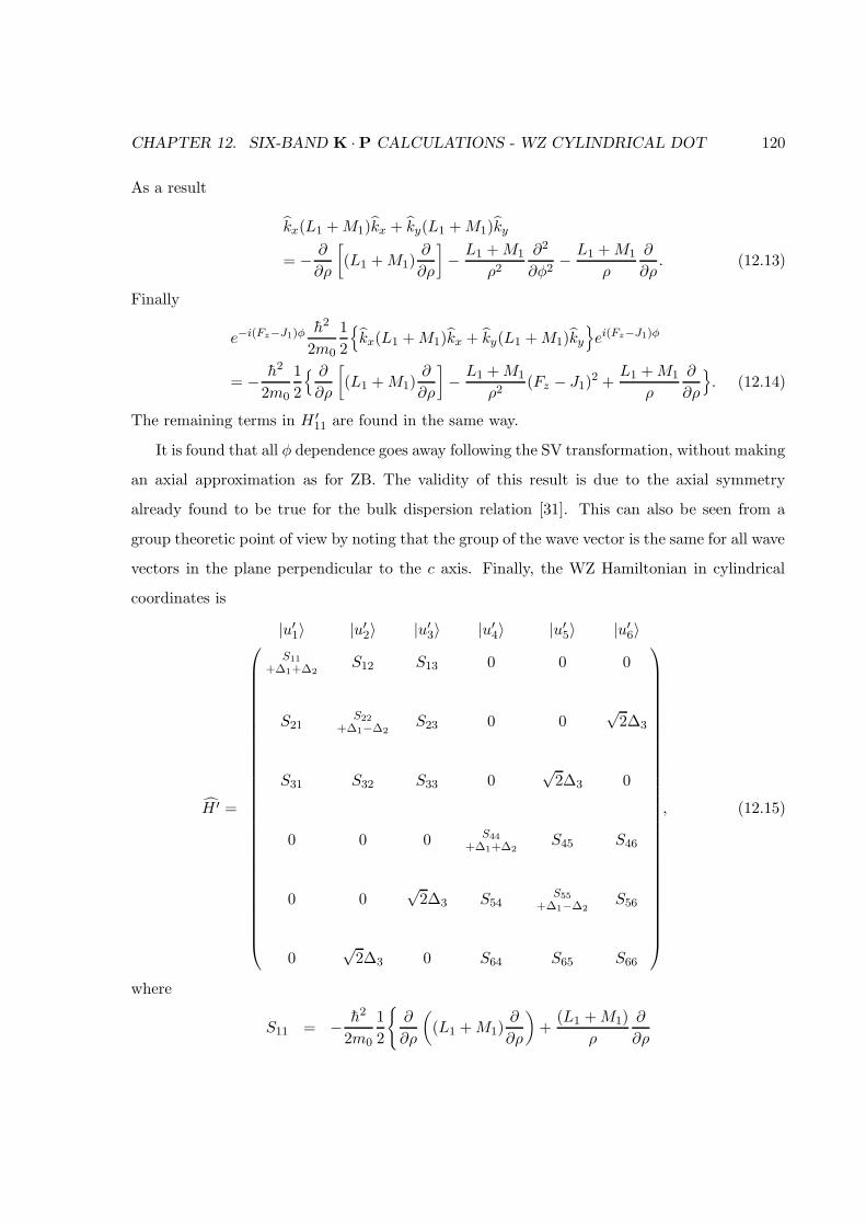
CHAPTER 12. SIX-BAND K ·P CALCULATIONS - WZ CYLINDRICAL DOT 120
As a result
kx(L1 +M1)kx + ky(L1 +M1)ky
= − ∂
∂ρ
[(L1 +M1)
∂
∂ρ
]− L1 +M1
ρ2
∂2
∂φ2− L1 +M1
ρ
∂
∂ρ. (12.13)
Finally
e−i(Fz−J1)φ h2
2m0
1
2
kx(L1 +M1)kx + ky(L1 +M1)ky
ei(Fz−J1)φ
= − h2
2m0
1
2
∂∂ρ
[(L1 +M1)
∂
∂ρ
]− L1 +M1
ρ2(Fz − J1)
2 +L1 +M1
ρ
∂
∂ρ
. (12.14)
The remaining terms in H ′11 are found in the same way.
It is found that all φ dependence goes away following the SV transformation, without making
an axial approximation as for ZB. The validity of this result is due to the axial symmetry
already found to be true for the bulk dispersion relation [31]. This can also be seen from a
group theoretic point of view by noting that the group of the wave vector is the same for all wave
vectors in the plane perpendicular to the c axis. Finally, the WZ Hamiltonian in cylindrical
coordinates is
H ′ =
|u′1〉 |u′2〉 |u′3〉 |u′4〉 |u′5〉 |u′6〉S11
+∆1+∆2S12 S13 0 0 0
S21S22
+∆1−∆2S23 0 0
√2∆3
S31 S32 S33 0√
2∆3 0
0 0 0 S44
+∆1+∆2S45 S46
0 0√
2∆3 S54S55
+∆1−∆2S56
0√
2∆3 0 S64 S65 S66
, (12.15)
where
S11 = − h2
2m0
1
2
∂
∂ρ
((L1 +M1)
∂
∂ρ
)+
(L1 +M1)
ρ
∂
∂ρ

CHAPTER 12. SIX-BAND K ·P CALCULATIONS - WZ CYLINDRICAL DOT 121
+ 2∂
∂zM2
∂
∂z− (Fz − J1)
ρ
∂(N1 −N ′1)
∂ρ
− (Fz − J1)2
ρ2(L1 +M1)
, (12.16)
S22 = − h2
2m0
1
2
∂
∂ρ
((L1 +M1)
∂
∂ρ
)+
(L1 +M1)
ρ
∂
∂ρ
+ 2∂
∂zM2
∂
∂z+
(Fz − J2)
ρ
∂(N1 −N ′1)
∂ρ
− (Fz − J2)2
ρ2(L1 +M1)
, (12.17)
S33 = − h2
2m0
∂
∂ρ
(M3
∂
∂ρ
)+M3
ρ
∂
∂ρ
+∂
∂zL2
∂
∂z− (Fz − J3)
2
ρ2M3
, (12.18)
S12 =h2
2m0
1
2
∂
∂ρ
((L1 −M1)
∂
∂ρ
)
+ (Fz − J2)∂
∂ρ
((L1 −M1)
ρ·)
+ (Fz − J2 − 1)(L1 −M1)
ρ
∂
∂ρ
+(Fz − J2)(Fz − J2 − 1)
ρ2(L1 −M1)
, (12.19)
S21 =h2
2m0
1
2
∂
∂ρ
((L1 −M1)
∂
∂ρ
)
− (Fz − J1)∂
∂ρ
((L1 −M1)
ρ·)
− (Fz − J1 + 1)(L1 −M1)
ρ
∂
∂ρ
+(Fz − J1)(Fz − J1 + 1)
ρ2(L1 −M1)
, (12.20)
S13 =h2
2m0
1√2
∂
∂ρ
(N2
∂
∂z
)+
∂
∂z
(N ′
2
∂
∂ρ
)
+ (Fz − J3)
[∂
∂z
(N ′
2
ρ·)
+N2
ρ
∂
∂z
], (12.21)
S31 =h2
2m0
1√2
∂
∂ρ
(N ′
2
∂
∂z
)+
∂
∂z
(N2
∂
∂ρ
)
CHAPTER 12. SIX-BAND K ·P CALCULATIONS - WZ CYLINDRICAL DOT 122
− (Fz − J1)
[∂
∂z
(N2
ρ·)
+N ′
2
ρ
∂
∂z
], (12.22)
S23 = − h2
2m0
1√2
∂
∂ρ
(N2
∂
∂z
)+
∂
∂z
(N ′
2
∂
∂ρ
)
− (Fz − J3)
[∂
∂z
(N ′
2
ρ·)
+N2
ρ
∂
∂z
], (12.23)
S32 = − h2
2m0
1√2
∂
∂ρ
(N ′
2
∂
∂z
)+
∂
∂z
(N2
∂
∂ρ
)
+ (Fz − J2)
[∂
∂z
(N2
ρ·)
+N ′
2
ρ
∂
∂z
], (12.24)
S44 = − h2
2m0
1
2
∂
∂ρ
((L1 +M1)
∂
∂ρ
)+
(L1 +M1)
ρ
∂
∂ρ
+ 2∂
∂zM2
∂
∂z+
(Fz − J4)
ρ
∂(N1 −N ′1)
∂ρ
− (Fz − J4)2
ρ2(L1 +M1)
, (12.25)
S55 = − h2
2m0
1
2
∂
∂ρ
((L1 +M1)
∂
∂ρ
)+
(L1 +M1)
ρ
∂
∂ρ
+ 2∂
∂zM2
∂
∂z− (Fz − J5)
ρ
∂(N1 −N ′1)
∂ρ
− (Fz − J5)2
ρ2(L1 +M1)
, (12.26)
S66 = − h2
2m0
∂
∂ρ
(M3
∂
∂ρ
)+M3
ρ
∂
∂ρ
+∂
∂zL2
∂
∂z− (Fz − J6)
2
ρ2M3
, (12.27)
S45 =h2
2m0
1
2
∂
∂ρ
((L1 −M1)
∂
∂ρ
)
− (Fz − J5)∂
∂ρ
((L1 −M1)
ρ·)
− (Fz − J5 + 1)(L1 −M1)
ρ
∂
∂ρ
+(Fz − J5)(Fz − J5 + 1)
ρ2(L1 −M1)
, (12.28)
S54 =h2
2m0
1
2
∂
∂ρ
((L1 −M1)
∂
∂ρ
)
CHAPTER 12. SIX-BAND K ·P CALCULATIONS - WZ CYLINDRICAL DOT 123
+ (Fz − J4)∂
∂ρ
((L1 −M1)
ρ·)
+ (Fz − J4 − 1)(L1 −M1)
ρ
∂
∂ρ
+(Fz − J4)(Fz − J4 − 1)
ρ2(L1 −M1)
, (12.29)
S46 = − h2
2m0
1√2
∂
∂ρ
(N2
∂
∂z
)+
∂
∂z
(N ′
2∂
∂ρ
)
− (Fz − J6)
[∂
∂z
(N ′
2·ρ
)+N2
ρ
∂
∂z
], (12.30)
S56 =h2
2m0
1√2
∂
∂ρ
(N2
∂
∂z
)+
∂
∂z
(N ′
2
∂
∂ρ
)
+ (Fz − J6)
[∂
∂z
(N ′
2·ρ
)+N2
ρ
∂
∂z
], (12.31)
S64 = − h2
2m0
1√2
∂
∂ρ
(N ′
2
∂
∂z
)+
∂
∂z
(N2
∂
∂ρ
)
+ (Fz − J4)
[∂
∂z
(N2·ρ
)+N ′
2
ρ
∂
∂z
], (12.32)
S65 =h2
2m0
1√2
∂
∂ρ
(N ′
2
∂
∂z
)+
∂
∂z
(N2
∂
∂ρ
)
− (Fz − J5)
[∂
∂z
(N2·ρ
)+N ′
2
ρ
∂
∂z
], (12.33)
where Jn ≡ Jzn. Note that in general Sij 6= S†ji.
Xia et al. [101, 102, 103] have added to the Hamiltonian (12.2) a term linear in k.
H(linear)k =
h2
2m0
0 0 Akx
0 0 Aky
Akx Aky 0
. (12.34)
In cylindrical coordinates this linear contribution is
S(linear)31 =
h2
2m0
− A√
2
∂
∂ρ+
A√2
Fz − J1
ρ
, (12.35)
S(linear)13 =
h2
2m0
− A√
2
∂
∂ρ− A√
2
Fz − J3
ρ
, (12.36)
S(linear)23 =
h2
2m0
A√2
∂
∂ρ− A√
2
Fz − J3
ρ
, (12.37)
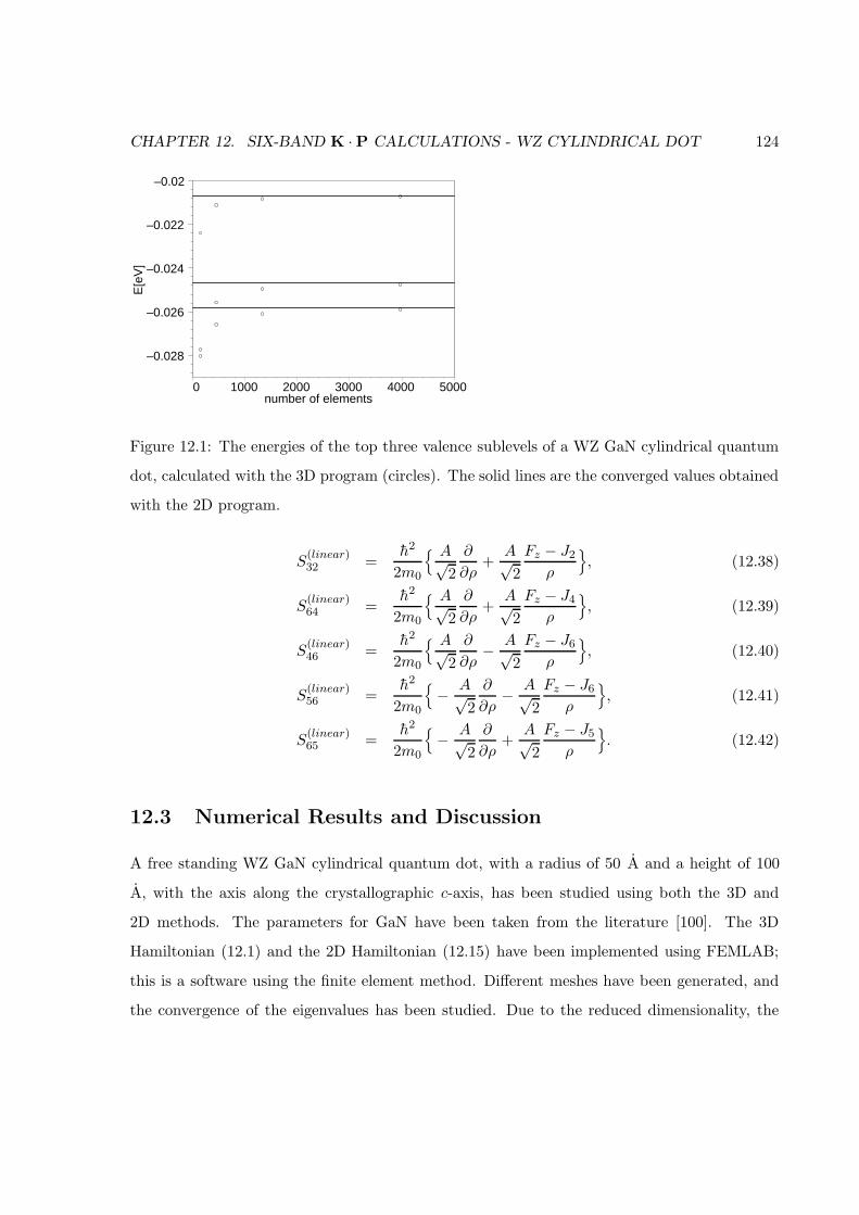
CHAPTER 12. SIX-BAND K ·P CALCULATIONS - WZ CYLINDRICAL DOT 124
–0.028
–0.026
–0.024
–0.022
–0.02
E[e
V]
0 1000 2000 3000 4000 5000number of elements
Figure 12.1: The energies of the top three valence sublevels of a WZ GaN cylindrical quantum
dot, calculated with the 3D program (circles). The solid lines are the converged values obtained
with the 2D program.
S(linear)32 =
h2
2m0
A√2
∂
∂ρ+
A√2
Fz − J2
ρ
, (12.38)
S(linear)64 =
h2
2m0
A√2
∂
∂ρ+
A√2
Fz − J4
ρ
, (12.39)
S(linear)46 =
h2
2m0
A√2
∂
∂ρ− A√
2
Fz − J6
ρ
, (12.40)
S(linear)56 =
h2
2m0
− A√
2
∂
∂ρ− A√
2
Fz − J6
ρ
, (12.41)
S(linear)65 =
h2
2m0
− A√
2
∂
∂ρ+
A√2
Fz − J5
ρ
. (12.42)
12.3 Numerical Results and Discussion
A free standing WZ GaN cylindrical quantum dot, with a radius of 50 A and a height of 100
A, with the axis along the crystallographic c-axis, has been studied using both the 3D and
2D methods. The parameters for GaN have been taken from the literature [100]. The 3D
Hamiltonian (12.1) and the 2D Hamiltonian (12.15) have been implemented using FEMLAB;
this is a software using the finite element method. Different meshes have been generated, and
the convergence of the eigenvalues has been studied. Due to the reduced dimensionality, the
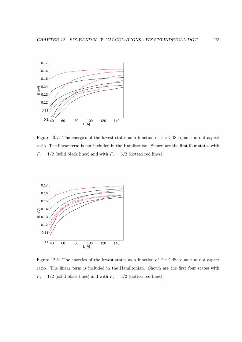
CHAPTER 12. SIX-BAND K ·P CALCULATIONS - WZ CYLINDRICAL DOT 125
0.1
0.11
0.12
0.13
0.14
0.15
0.16
0.17
E [e
V]
40 60 80 100 120 140L [A]
Figure 12.2: The energies of the lowest states as a function of the CdSe quantum dot aspect
ratio. The linear term is not included in the Hamiltonian. Shown are the first four states with
Fz = 1/2 (solid black lines) and with Fz = 3/2 (dotted red lines).
0.1
0.11
0.12
0.13
0.14
0.15
0.16
0.17
E [e
V]
40 60 80 100 120 140L [A]
Figure 12.3: The energies of the lowest states as a function of the CdSe quantum dot aspect
ratio. The linear term is included in the Hamiltonian. Shown are the first four states with
Fz = 1/2 (solid black lines) and with Fz = 3/2 (dotted red lines).
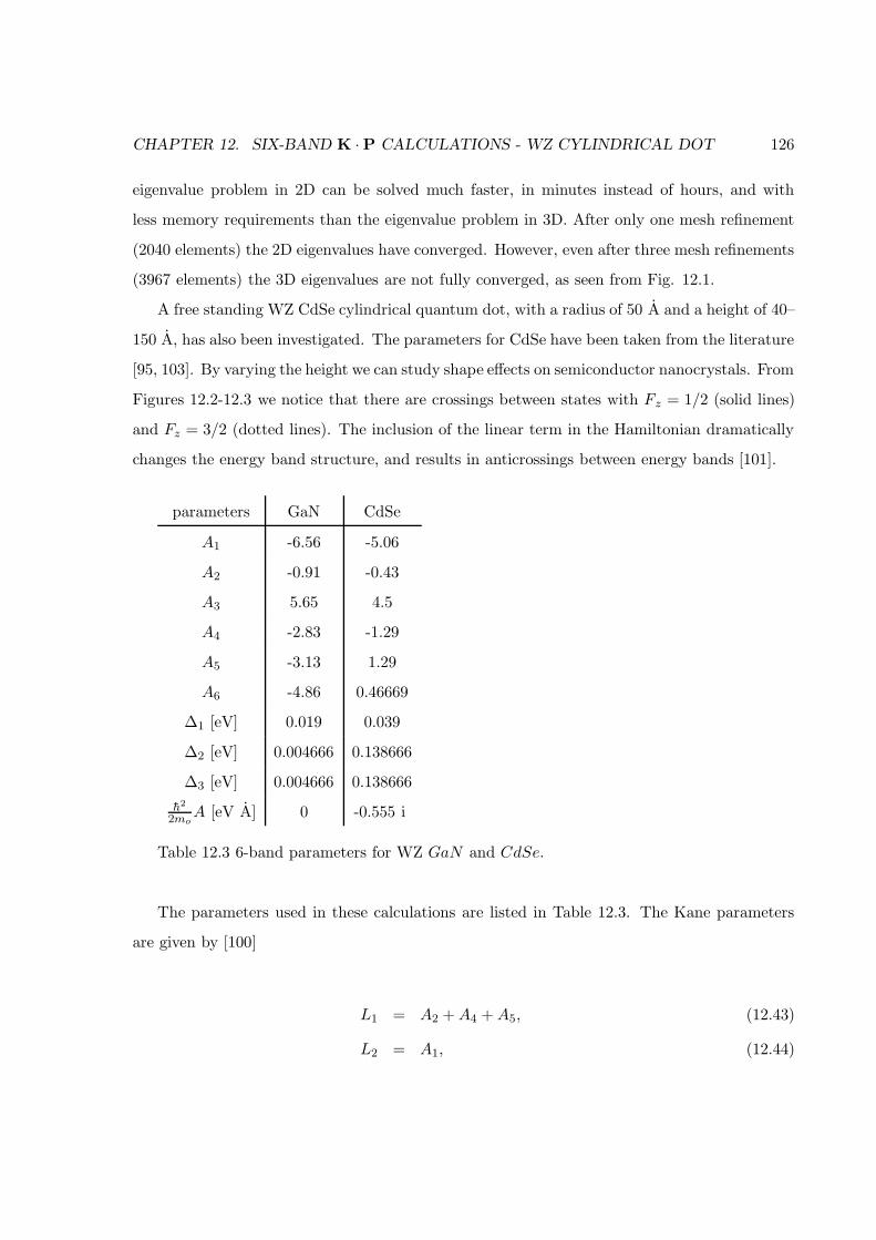
CHAPTER 12. SIX-BAND K ·P CALCULATIONS - WZ CYLINDRICAL DOT 126
eigenvalue problem in 2D can be solved much faster, in minutes instead of hours, and with
less memory requirements than the eigenvalue problem in 3D. After only one mesh refinement
(2040 elements) the 2D eigenvalues have converged. However, even after three mesh refinements
(3967 elements) the 3D eigenvalues are not fully converged, as seen from Fig. 12.1.
A free standing WZ CdSe cylindrical quantum dot, with a radius of 50 A and a height of 40–
150 A, has also been investigated. The parameters for CdSe have been taken from the literature
[95, 103]. By varying the height we can study shape effects on semiconductor nanocrystals. From
Figures 12.2-12.3 we notice that there are crossings between states with Fz = 1/2 (solid lines)
and Fz = 3/2 (dotted lines). The inclusion of the linear term in the Hamiltonian dramatically
changes the energy band structure, and results in anticrossings between energy bands [101].
parameters GaN CdSe
A1 -6.56 -5.06
A2 -0.91 -0.43
A3 5.65 4.5
A4 -2.83 -1.29
A5 -3.13 1.29
A6 -4.86 0.46669
∆1 [eV] 0.019 0.039
∆2 [eV] 0.004666 0.138666
∆3 [eV] 0.004666 0.138666
h2
2moA [eV A] 0 -0.555 i
Table 12.3 6-band parameters for WZ GaN and CdSe.
The parameters used in these calculations are listed in Table 12.3. The Kane parameters
are given by [100]
L1 = A2 +A4 +A5, (12.43)
L2 = A1, (12.44)
CHAPTER 12. SIX-BAND K ·P CALCULATIONS - WZ CYLINDRICAL DOT 127
M1 = A2 +A4 −A5, (12.45)
M2 = A1 +A3, (12.46)
M3 = A2, (12.47)
N1 = 1 + 3A5 −A2 −A4, (12.48)
N ′1 = −1 +A2 +A4 −A5, (12.49)
N2 = 1 −A1 −A3 +√
2A6, (12.50)
N ′2 = −1 +A1 +A3. (12.51)
In CdSe nanocrystals with a radius of 15 A and a gelcap shape a crossing between the
lowest two valence sublevels appears at an aspect ratio of 1.25 [86]. There are also some
experimental studies of the transition from 3D to 2D confinement in CdSe quantum rods [86,
104]. Theoretical work on the electronic properties of the transition reported so far include
empirical pseudopotential calculations on a rather artificial shape [86], and k ·p calculations for
cylindrical ZB structures [88, 105] and for spheroidal WZ structures [103]. We hope that our
new formulation for studying the electronic structure of wurzite quantum dots with cylindrical
symmetry will be a very useful tool in this important research area.
12.4 Conclusions
We have extended the Sercel-Vahala technique to WZ heterostructures with cylindrical sym-
metry and shown this to be an exact result. This is crucial for applications in enabling greatly
decreased computational resources. We have studied GaN and CdSe cylindrical quantum dots,
calculating the effect of the aspect ratio on energy levels and wavefunctions.
Chapter 13
Summary
A multiband Burt-Foreman formulation of the k · p theory was successfully carried out for
arbitrary nanostructures. This went beyond previous work in the computation of optical matrix
elements for ZB quantum wells, in the investigation of shape effects in quantum dots, and in a
new formulation for WZ cylindrical nanostructures along the [0001] direction. We have shown
that the one-band k · p equation for an elliptical quantum dot embedded in a finite barrier
material is not separable. We have demonstrated a possible electron localization in a nanowire
superlattice in a barrier material, using a full numerical solution to the one band k · p equation.
The difference between bandstructures and momentum matrix elements calculated with both
the Burt-Foreman and the Luttinger-Kohn Hamiltonians has been shown to be small, especially
when using an 8-band model. We have found that the axial approximation was not required
when the 6-band Burt-Foreman theory was extended to cylindrical coordinates using the Sercel-
Vahala transformation for WZ semiconductors. This is different from the results of others on
corresponding ZB nanostructures.
Future work may include the effect of strain on bandstructures and optical properties. From
a computational point of view we need newer and improved algorithms to solve the secular
equation for a very large and sparse matrix.
128
Bibliography
[1] P. S. Zory jr. Quantum Well Lasers. Academic, Boston, 1993.
[2] P. Harrison. Quantum Wells, Wires and Dots. Wiley, New York, 1999.
[3] S. Nakamura, S. Pearton, and G. Fasol. The Blue Laser Diode. Springer, New York, 2000.
[4] J. M. Luttinger and W. Kohn. Motion of electrons and holes in perturbed periodic fields.
Phys. Rev., 97(4):869–883, Feb 1955.
[5] M. G. Burt. An exact formulation of the envelope function method for the determination
of electronic states in semiconductor microstructures. Semicond. Science and Technology,
2:460–462, 1987.
[6] M. G. Burt. An exact formulation of the envelope function method for the determination
of electronic states in semiconductor microstructures (erratum). Semicond. Science and
Technology, 2:701, 1987.
[7] M. G. Burt. An exact formulation of the envelope function method for the determination
of electronic states in semiconductor microstructures. Semicond. Science and Technology,
3:739–753, 1988.
[8] M. G. Burt. A new effective-mass equation for microstructures. Semicond. Science and
Technology, 3:1224–1226, 1988.
[9] M. G. Burt. Exact envelope function equations for microstructures and the particle in a
box model. In A. Abram and M. Jaros, editors, Bandstructure Engineering in Semicon-
129
BIBLIOGRAPHY 130
ductor Microstructures, NATO ASI Series B, vol. 189, pages 99–109. Plenum, New York,
1989.
[10] M. G. Burt. The justification for applying the effective-mass approximation to microstruc-
tures. J. Phys.: Condens. Matter, 4:6651–6690, 1992.
[11] B. A. Foreman. Effective-mass hamiltonian and boundary conditions for the valence bands
of semiconductor microstructures. Phys. Rev. B, 48(7):4964–4967, Aug 1993.
[12] B. A. Foreman. Elimination of spurious solutions from eight-band k · p theory. Phys.
Rev. B, 56(20):R12748–R12751, Nov 1997.
[13] W. E. Buhro and V. L. Colvin. Shape matters. Nature Mat., 2:138–139, 2003.
[14] P.Y. Yu and M. Cardona. Fundamentals of Semiconductors. Springer, 1999.
[15] P.T. Landsberg. Solid State Theory. Wiley, 1969, p. 252.
[16] G. Dresselhaus, A. F. Kip, and C. Kittel. Cyclotron resonance of electrons and holes in
silicon and germanium crystals. Phys. Rev., 98(2):368–384, Apr 1955.
[17] E. O. Kane. Energy band structure in p-type germanium and silicon. J. Phys. Chem.
Sol., 1:82–99, 1956.
[18] E. O. Kane. Band structure of indium antimonide. J. Phys. Chem. Sol., 1:249–261, 1957.
[19] E. O. Kane. The semi-empirical approach to band structure. In H. Brooks, editor,
Advances in Semiconductor Science, pages 38–44. Pergamon, New York, 1959.
[20] E. O. Kane. The k · p method. In R. K. Willardson and A. C. Beer, editors, Physics of
III-V Compounds, volume 1 of Semiconductors and Semimetals, chapter 3, pages 75–100.
Academic, New York, 1966.
[21] E. O. Kane. Band structure of narrow gap semiconductors. In W. Zawadzki, editor,
Narrow Gap Semiconductors, pages 13–31. Springer-Verlag, Berlin, 1980.
BIBLIOGRAPHY 131
[22] E. O. Kane. Energy band theory. In T. S. Moss, editor, Handbook on Semiconductors,
pages 193–217. North-Holland, Amsterdam, 1982.
[23] P.-O. Lowdin. A note on quantum-mechanical perturbation theory. J. Chem. Phys.,
19(11):1396–1401, Nov 1951.
[24] A. T. Meney, B. Gonul, and E. P. O’Reilly. Evaluation of various approximations used in
the envelope-function method. Phys. Rev. B, 50(15):10893–10904, Oct 1994.
[25] F. Mireles and S. E. Ulloa. Ordered Hamiltonian and matching conditions for hetero-
junctions with wurtzite symmetry: GaN/AlxGa1−xN quantum wells. Phys. Rev. B,
60(19):13659–13667, 1999.
[26] F. Mireles and S. E. Ulloa. Strain and crystallographic orientation effects on the valence
subbands of wurtzite quantum wells. Phys. Rev. B, 62(4):2562–2572, 2000.
[27] B. Lassen, L.C. Lew Yan Voon, M. Willatzen, and R. Melnik. Exact envelope-function
theory versus symmetrized hamiltonian for quantum wires: a comparison. Solid State
Com., 132(3-4):141–149, Oct 2004.
[28] E. P. Pokatilov, V. A. Fonoberov, V. M. Fomin, and J. T. Devreese. Development of
an eight-band theory for quantum dot heterostructures. Phys. Rev. B, 64(24):245328–1–
245328–16, 2001.
[29] F. Szmulowicz. Derivation of a general expression for the momentum matrix elements
within the envelope-function approximation. Phys. Rev. B, 51(3):1613, Jan 1995.
[30] F. Szmulowicz and G. J. Brown. Calculation and photoresponse measurement of the
bound-to-continuum infrared absorption in p-type GaAs/AlxGa1−xAs quantum wells.
Phys. Rev. B, 51(19):13203–13220, May 1995.
[31] S. L. Chuang and C. S. Chang. k · p method for strained wurtzite semiconductors. Phys.
Rev. B, 54(4):2491–2504, Jul 1996.
BIBLIOGRAPHY 132
[32] M. Grundmann, O. Stier, and D. Bimberg. InAs/GaAs pyramidal quantum dots: Strain
distribution, optical phonons, and electronic structure. Phys. Rev. B, 52:11969–11980,
1995.
[33] G. L. Bir and G. E. Pikus. Symmetry and Strain-Induced Effects in Semiconductors.
Wiley, New York, 1975.
[34] L. C. Lew Yan Voon, C. Galeriu, and M. Willatzen. Comment on: ”Confined states
in two-dimensional flat elliptic quantum dots and elliptic quantum wires”. Physica E,
18:547–549, 2003.
[35] M. van den Broek and F. M. Peeters. Confined states in two-dimensional flat elliptic
quantum dots and elliptic quantum wires. Physica E, 11:345–355, 2001.
[36] C. Galeriu, L. C. Lew Yan Voon, R. N. Melnik, and M. Willatzen. Modeling a nanowire
superlattice using the finite difference method in cylindrical polar coordinates. Comp.
Phys. Commun., 157:147–159, 2004.
[37] M. S. Gudiksen, L. J. Lauhon, J. Wang, D. C. Smith, and C. M. Lieber. Growth of
nanowire superlattice structures for nanoscale photonics and electronics. Nature, 415:617–
620, Feb 2002.
[38] R. Solanki, J. Huo, J. L. Freeouf, and B. Miner. Atomic layer deposition of ZnSe/CdSe
superlattice nanowires. App. Phys. Lett., 81(20):3864–3866, Nov 2002.
[39] L. C. Lew Yan Voon and M. Willatzen. Electron states in modulated nanowires. J. App.
Phys., 93:9997–10000, 2003.
[40] Y.-C. Chang and R. B. James. Saturation of intersubband transitions in p-type semicon-
ductor quantum wells. Phys. Rev. B, 39(17):12672–12681, Jun 1989.
[41] L. C. Lew Yan Voon, M. Willatzen, M. Cardona, and N. E. Christensen. Terms linear in k
in the band structure of wurtzite-type semiconductors. Phys. Rev. B, 53(16):10703–10714,
1996.
BIBLIOGRAPHY 133
[42] K. J. Vahala and P. C. Sercel. Application of a total-angular-momentum basis to quantum-
dot band structure. Phys. Rev. Lett., 65(2):239–242, Jul 1990.
[43] P. C. Sercel and K. J. Vahala. Analytical technique for determining quantum-wire and
quantum-dot band structure in the multiband envelope-function representation. Phys.
Rev. B, 42(6):3690–3711, Aug 1990.
[44] L. Landau and E. Lifchitz. Mecanique Quantique. Mir, Moscow, 1966, p. 415.
[45] J.J. Sakurai. Modern Quantum Mechanics. Addison-Wesley, 1994, p. 239.
[46] G.F. Koster, J.O. Dimmock, R.G. Wheeler, and H. Statz. Properties of the thirty-two
point groups. MIT Press, 1963.
[47] L. C. Lew Yan Voon. Electronic and Optical Properties of Semiconductors: A Study Based
on the Empirical Tight Binding Model. Dissertations.com, 1997, p. 176.
[48] J.J. Sakurai. Modern Quantum Mechanics. Addison-Wesley, 1994, p. 164.
[49] G. Dresselhaus. Spin-orbit coupling effects in zinc blende structures. Phys. Rev.,
100(2):580–586, 1955.
[50] G. Bastard. Wave Mechanics Applied to Semiconductor Heterostructures. Halsted Press,
1988.
[51] D.G. Seiler, B.D. Bajaj, and A.E. Stephens. Inversion-asymmetry splitting of the con-
duction band in InSb. Phys. Rev. B, 16(6):2822–2833, Sep 1977.
[52] L. Landau and E. Lifchitz. Mecanique Quantique. Mir, Moscow, 1966, p. 162.
[53] R. Eppenga, M.F.H. Schuurmans, and S. Colak. New k · p theory for GaAs/Ga1−xAlxAs
- type quantum wells. Phys. Rev. B, 36(3):1554–1564, Jul 1987.
[54] D. Gershoni, C. H. Henry, and G.A. Baraff. Calculating the optical properties of multi-
dimensional heterostructures: Application to the modeling of quaternary quantum well
lasers. IEEE J. Quantum Elec., 29(9):2433–2450, Sep 1993.
BIBLIOGRAPHY 134
[55] S. A. Stoklitsky, Q. X. Zhao, P. O. Holtz, B. Monemar, and T. Lundstrom. Optical
intervalence-subband transitions in strained p-type In1−xGaxAs/InP quantum wells. J.
App. Phys., 77(10):5256–5262, 1995.
[56] O. Stier and D. Bimberg. Modeling of strained quantum wires using eight-band k · ptheory. Phys. Rev. B, 55(12):7726–7732, Mar 1997.
[57] O. Stier, M. Grundmann, and D. Bimberg. Electronic and optical properties of strained
quantum dots modeled by 8-band k · p theory. Phys. Rev. B, 59(8):5688–5701, Feb 1999.
[58] G. Shechter and L. D. Shvartsman. Theory of bound-to-continuum infrared absorption
in p-type quantum wells based on a mapping of the continuum spectrum. Phys. Rev. B,
58(7):3941–3953, 1998.
[59] P. Enders, A. Brwolff, M. Woerner, and D. Suisky. k · p theory of energy bands, wave
functions, and optical selection rules in strained tetrahedral semiconductors. Phys. Rev.
B, 51(23):16695–16704, Jun 1995.
[60] K.I. Kolokolov, S.D. Beneslavski, N.Y. Minina, and A.M. Savin. Far-infrared intersubband
absorption in p-type GaAs/AlxGa1−xAs single heterojunctions under uniaxial compres-
sion. Phys. Rev. B, 63(19):195308–1–195308–6, May 2001.
[61] L. Landau and E. Lifchitz. Theorie de L’ Elasticite. Mir, Moscow, 1967.
[62] Herbert Reismann and Peter S. Pawlik. Elasticity, Theory and Applications. John Wiley,
New York, 1980.
[63] A. S. Saada. Elasticity Theory and Applications. Krieger, Malabar, 1993.
[64] A. K. Ghatak, K. Thyagarajan, and M. R. Shenoy. A novel numerical technique for
solving the one-dimensional Schrodinger equation using matrix approach — application
to quantum well structures. IEEE J. Quantum Elec., 24(8):1524–1531, Aug 1988.
[65] K. Nakamura, A. Shimizu, M. Koshiba, and K. Hayata. Finite-element analysis of quan-
tum wells of arbitrary semiconductors with arbitrary potential profiles. IEEE J. Quantum
Elec., 25(5):889–895, May 1989.
BIBLIOGRAPHY 135
[66] I.-H. Tan, G. L. Snider, L. D. Chang, and E. L. Hu. A self-consistent solution of
Schrodinger-Poisson equations using a nonuniform mesh. J. App. Phys., 68(8):4071–7,
Oct 1990.
[67] M. Tsetseri and G. P. Triberis. A study of the ground state of quantum wires using the
finite difference method. Superlattices and Microstructures, 32(1):79–90, July 2002.
[68] D. El-Moghraby, R. G. Johnson, and P. Harrison. Calculating modes of quantum wire and
dot systems using a finite differencing technique. Comput. Phys. Comm., 150(3):235–246,
Feb 2003.
[69] D. L. Mathine, S. K. Myjak, and G. N. Maracas. A computational Fourier series solution of
the BenDaniel-Duke Hamiltonian for arbitrary shaped quantum wells. IEEE J. Quantum
Elec., 31(7):1216, Jul 1995.
[70] G. Lamouche and Y. Lepine. Ground state of a quantum disk by the effective-index
method. Phys. Rev. B, 51(3):1950–1953, Jan 1995.
[71] S. L. Chuang and C. S. Chang. A band-structure model of strained quantum-well wurtzite
semiconductors. Semicond. Sci. Technol., 12:252–263, 1997.
[72] L. C. Lew Yan Voon and M. Willatzen. Angular confinement, non-integral quantum
numbers, and controllable degeneracies. Europhys. Lett., 62:299–305, 2003.
[73] P.M. Morse and H. Feshbach. Methods of Theoretical Physics. McGraw-Hill, New York,
1953.
[74] R. Lehoucq, D.C. Sorensen, and C. Yang. Arpack User’s Guide. SIAM, 1998.
[75] Y. Li, J.-L. Liu, O. Voskoboynikov, C. P. Lee, and S. M. Sze. Electron energy level calcu-
lations for cylindrical narrow gap semiconductor quantum dot. Comput. Phys. Comm.,
140(3):399–404, Nov 2001.
[76] Y. Li, O. Voskoboynikov, C. P. Lee, and S. M. Sze. Computer simulation of electron
energy levels for different shape InAs/GaAs semiconductor quantum dots. Comput. Phys.
Comm., 141(1):66–72, Nov 2001.
BIBLIOGRAPHY 136
[77] Y. Li, O. Voskoboynikov, C. P. Lee, and S. M. Sze. Energy and coordinate dependent
effective mass and confined electron states in quantum dots. Solid State Comm., 120(2-
3):79–83, Sep 2001.
[78] Y. Wu, R. Fan, and P. Yang. Block-by-block growth of single-crystalline Si/SiGe super-
lattice nanowires. Nano Lett., 2:83–86, 2002.
[79] M. T. Bjork, B. J. Ohlsson, T. Sass, A. I. Persson, C. Thelander, M. H. Magnusson,
K. Deppert, L. R. Wallenberg, and L. Samuelson. One-dimensional steeplechase for elec-
trons realized. Nano Lett., 2:87–89, 2002.
[80] M. Kawamura, N. Paul, V. Cherepanov, and B. Voigtlander. Nanowires and nanorings
at the atomic level. Phys. Rev. Lett., 91(9):096102–1–096102–4, 2003.
[81] R. M. Kolbas and N. Holonyak Jr. Man-made quantum wells: A new perspective on the
finite square-well problem. Am. J. Phys, 52(5):431–437, May 1984.
[82] R. Verzicco and P. Orlandi. A finite-difference scheme for three-dimensional incompress-
ible flows in cylindrical coordinates. J. Comput. Phys., 123(2):402–414, Feb 1996.
[83] H.-S. Cho and P. R. Prucnal. New formalism of the kronig-penney model with application
to superlattices. Phys. Rev. B, 36(6):3237–3242, Aug 1987.
[84] L. C. Lew Yan Voon. Discontinuities in the effective-mass equation. Superlattices and
Microstructures, 31(6):269–276, 2002.
[85] E. Kapon, D. M. Hwang, and R. Bhat. Stimulated emission in semiconductor quantum
wire heterostructures. Phys. Rev. Lett., 63(4):430–433, 1989.
[86] J. Hu, L. Li, W. Yang, L. Manna, L. Wang, and A. P. Alivisatos. Linearly polarized
emission from colloidal semiconductor quantum rods. Science, 292:2060–2063, Jun 2001.
[87] L. Li, J. Hu, W. Yang, and A. P. Alivisatos. Band gap variation of size- and shape-
controlled colloidal CdSe quantum rods. Nano Lett., 1(7):349–351, 2001.
BIBLIOGRAPHY 137
[88] D. Katz, T. Wizansky, O. Millo, E. Rothenberg, T. Mokari, and U. Banin. Size-dependent
tunneling and optical spectroscopy of CdSe quantum rods. Phys. Rev. Lett., 89(8):086801–
1–086801–4, 2002.
[89] Y. Wang, L. Zhang, C. Liang, G. Wang, and X. Peng. Catalitic growth and photolumi-
nescence properties of semiconductor single-crystal ZnS nanowires. Chem. Phys. Lett.,
357:314–318, May 2002.
[90] Z. R. Tian, J. A. Voigt, J. Liu, B. McKenzie, M. J. McDermott, M. A. Rodriguez,
H. Konishi, and H. Xu. Complex and oriented ZnO nanostructures. Nature Materials,
2:821–826, Dec 2003.
[91] M. H. Huang, S. Mao, H. Feick, H. Yan, Y. Wu, H. Kind, E. Weber, R. Russo, and
P. Yang. Room-temperature ultraviolet nanowire nanolasers. Science, 292:1897–1899,
Jun 2001.
[92] Q. L. Liu, T. Tanaka, J. Q. Hu, F. F. Xu, and T. Sekiguchi. Green emission from c-axis
oriented AlN nanorods doped with Tb. Appl. Phys. Lett., 83(24):4939–4941, Dec 2003.
[93] J. C. Johnson, H. Choi, K. P. Knutsen, R. D. Schaller, P. Yang, and R. J. Saykally. Single
gallium nitride nanowires lasers. Nature Materials, 1:106–110, Oct 2002.
[94] E. I. Rashba. Symmetry of energy bands in crystals of wurtzite type. Sov. Phys. Solid
State, 1:368–380, 1959.
[95] J.-B. Jeon, Y. M. Sirenko, K. W. Kim, M. A. Littlejohn, and M. A. Stroscio. Valence
band parameters of wurtzite materials. Solid State Comm., 99(6):423–426, 1996.
[96] A. D. Andreev and E. P. OReilly. Theory of the electronic structure of GaN/AlN hexag-
onal quantum dots. Phys. Rev. B, 62(23):15851–15870, Dec 2000.
[97] J. Planelles, W. Jaskolski, and J. I. Aliaga. Energy structure of quantum rings in a
magnetic field. Phys. Rev. B, 65(3):033306–1–033306–4, 2002.
[98] F. B. Pedersen and Y.-C. Chang. Energy levels of one and two holes in parabolic quantum
dots. Phys. Rev. B, 53(3):1507–1516, Jan 1996.
BIBLIOGRAPHY 138
[99] X. Duan and C. M. Lieber. General synthesis of compound semiconductor nanowires.
Adv. Mat., 12(4):298–301, 2000.
[100] V. A. Fonoberov and A. A. Balandin. Excitonic properties of strained wurtzite and zinc-
blende GaN/AlxGa1−xN quantum dots. J. Appl. Phys., 94(11):7178–7186, Nov 2003.
[101] J.-B. Xia, K. W. Cheah, X.-L. Wang, D.-Z. Sun, and M.-Y. Kong. Energy bands and
acceptor binding energies of GaN. Phys. Rev. B, 59(15):10119–10124, Apr 1999.
[102] J.-B. Xia and J. Li. Electronic structure of quantum spheres with wurtzite structure.
Phys. Rev. B, 60(16):11540–11544, Oct 1999.
[103] X.-Z. Li and J.-B. Xia. Electronic structure and optical properties of quantum rods with
wurtzite structure. Phys. Rev. B, 66(11):115316–1–115316–6, Sep 2002.
[104] H. Yu, J. Li, R. A. Loomis, P. C. Gibbons, L.-W. Wang, and W. E. Buhro. Cadmium
selenide quantum wires and the transition from 3D to 2D confinement. J. Am. Chem.
Soc., 125:16168–16169, 2003.
[105] L. C. Lew Yan Voon, R. Melnik, B. Lassen, and M. Willatzen. Influence of aspect ratio
on the lowest states of quantum rods. Nano Lett., 4(2):289–292, 2004.