JWCL232 c11 401-448.qxd 1/15/10 5:04 PM Page 401...
112
401 11 Simple Linear Regression and Correlation The space shuttle Challenger accident in January 1986 was the result of the failure of O-rings used to seal field joints in the solid rocket motor due to the extremely low ambi- ent temperatures at the time of launch. Prior to the launch there were data on the occur- rence of O-ring failure and the corresponding temperature on 24 prior launches or static firings of the motor. In this chapter we will see how to build a statistical model relating the probability of O-ring failure to temperature. This model provides a measure of the risk as- sociated with launching the shuttle at the low temperature occurring when Challenger was launched. (15 July 2009)—Space Shuttle Endeavour and its seven-member STS-127 crew head toward Earth orbit and rendezvous with the International Space Station Courtesy NASA CHAPTER OUTLINE 11-1 EMPIRICAL MODELS 11-2 SIMPLE LINEAR REGRESSION 11-3 PROPERTIES OF THE LEAST SQUARES ESTIMATORS 11-4 HYPOTHESIS TESTS IN SIMPLE LINEAR REGRESSION 11-4.1 Use of t-Tests 11-4.2 Analysis of Variance Approach to Test Significance of Regression 11-5 CONFIDENCE INTERVALS 11-5.1 Confidence Intervals on the Slope and Intercept 11-5.2 Confidence Interval on the Mean Response 11-6 PREDICTION OF NEW OBSERVATIONS 11-7 ADEQUACY OF THE REGRESSION MODEL 11-7.1 Residual Analysis 11-7.2 Coefficient of Determination (R 2 ) 11-8 CORRELATION 11-9 REGRESSION ON TRANSFORMED VARIABLES 11-10 LOGISTIC REGRESSION JWCL232_c11_401-448.qxd 1/15/10 5:04 PM Page 401
-
Upload
truonghuong -
Category
Documents
-
view
297 -
download
14
Transcript of JWCL232 c11 401-448.qxd 1/15/10 5:04 PM Page 401...

401
11Simple Linear Regression
and Correlation
The space shuttle Challenger accident in January 1986 was the result of the failure ofO-rings used to seal field joints in the solid rocket motor due to the extremely low ambi-ent temperatures at the time of launch. Prior to the launch there were data on the occur-rence of O-ring failure and the corresponding temperature on 24 prior launches or staticfirings of the motor. In this chapter we will see how to build a statistical model relating theprobability of O-ring failure to temperature. This model provides a measure of the risk as-sociated with launching the shuttle at the low temperature occurring when Challengerwas launched.
(15 July 2009)—SpaceShuttle Endeavour andits seven-member STS-127 crew headtoward Earth orbit andrendezvous with theInternational SpaceStation Courtesy NASA
CHAPTER OUTLINE
11-1 EMPIRICAL MODELS
11-2 SIMPLE LINEAR REGRESSION
11-3 PROPERTIES OF THE LEAST
SQUARES ESTIMATORS
11-4 HYPOTHESIS TESTS IN SIMPLE
LINEAR REGRESSION
11-4.1 Use of t-Tests
11-4.2 Analysis of Variance Approach
to Test Significance of Regression
11-5 CONFIDENCE INTERVALS
11-5.1 Confidence Intervals on the
Slope and Intercept
11-5.2 Confidence Interval on the
Mean Response
11-6 PREDICTION OF NEW
OBSERVATIONS
11-7 ADEQUACY OF THE REGRESSION
MODEL
11-7.1 Residual Analysis
11-7.2 Coefficient of Determination (R2)
11-8 CORRELATION
11-9 REGRESSION ON TRANSFORMED
VARIABLES
11-10 LOGISTIC REGRESSION
JWCL232_c11_401-448.qxd 1/15/10 5:04 PM Page 401

402 CHAPTER 11 SIMPLE LINEAR REGRESSION AND CORRELATION
LEARNING OBJECTIVES
After careful study of this chapter, you should be able to do the following:
1. Use simple linear regression for building empirical models to engineering and scientific data
2. Understand how the method of least squares is used to estimate the parameters in a linear
regression model
3. Analyze residuals to determine if the regression model is an adequate fit to the data or to see if
any underlying assumptions are violated
4. Test statistical hypotheses and construct confidence intervals on regression model parameters
5. Use the regression model to make a prediction of a future observation and construct an
appropriate prediction interval on the future observation
6. Apply the correlation model
7. Use simple transformations to achieve a linear regression model
11-1 EMPIRICAL MODELS
Many problems in engineering and the sciences involve a study or analysis of the relationshipbetween two or more variables. For example, the pressure of a gas in a container is related tothe temperature, the velocity of water in an open channel is related to the width of the chan-nel, and the displacement of a particle at a certain time is related to its velocity. In this last ex-ample, if we let d0 be the displacement of the particle from the origin at time t = 0 and v be thevelocity, then the displacement at time t is dt = d0 + vt. This is an example of a deterministiclinear relationship, because (apart from measurement errors) the model predicts displacementperfectly.
However, there are many situations where the relationship between variables is not deter-ministic. For example, the electrical energy consumption of a house ( y) is related to the sizeof the house (x, in square feet), but it is unlikely to be a deterministic relationship. Similarly,the fuel usage of an automobile ( y) is related to the vehicle weight x, but the relationship is nota deterministic one. In both of these examples the value of the response of interest y (energyconsumption, fuel usage) cannot be predicted perfectly from knowledge of the corresponding x.It is possible for different automobiles to have different fuel usage even if they weigh the same,and it is possible for different houses to use different amounts of electricity even if they are thesame size.
The collection of statistical tools that are used to model and explore relationships be-tween variables that are related in a nondeterministic manner is called regression analysis.Because problems of this type occur so frequently in many branches of engineering and sci-ence, regression analysis is one of the most widely used statistical tools. In this chapter wepresent the situation where there is only one independent or predictor variable x and the re-lationship with the response y is assumed to be linear. While this seems to be a simple sce-nario, there are many practical problems that fall into this framework.
For example, in a chemical process, suppose that the yield of the product is related tothe process-operating temperature. Regression analysis can be used to build a model topredict yield at a given temperature level. This model can also be used for process opti-mization, such as finding the level of temperature that maximizes yield, or for processcontrol purposes.
JWCL232_c11_401-448.qxd 1/15/10 5:36 PM Page 402

11-1 EMPIRICAL MODELS 403
As an illustration, consider the data in Table 11-1. In this table y is the purity of oxygenproduced in a chemical distillation process, and x is the percentage of hydrocarbons that arepresent in the main condenser of the distillation unit. Figure 11-1 presents a scatter diagramof the data in Table 11-1. This is just a graph on which each (xi, yi) pair is represented as a pointplotted in a two-dimensional coordinate system. This scatter diagram was produced byMinitab, and we selected an option that shows dot diagrams of the x and y variables along thetop and right margins of the graph, respectively, making it easy to see the distributions of theindividual variables (box plots or histograms could also be selected). Inspection of this scatterdiagram indicates that, although no simple curve will pass exactly through all the points, thereis a strong indication that the points lie scattered randomly around a straight line. Therefore, itis probably reasonable to assume that the mean of the random variable Y is related to x by thefollowing straight-line relationship:
where the slope and intercept of the line are called regression coefficients. While the mean ofY is a linear function of x, the actual observed value y does not fall exactly on a straight line.The appropriate way to generalize this to a probabilistic linear model is to assume that theexpected value of Y is a linear function of x, but that for a fixed value of x the actual value of Yis determined by the mean value function (the linear model) plus a random error term, say,
(11-1)Y ϭ 0 ϩ 1x ϩ ⑀
E1Y 0 x2 ϭ Y 0 x ϭ 0 ϩ 1x
Table 11-1 Oxygen and Hydrocarbon Levels
Observation Hydrocarbon Level PurityNumber x (%) y (%)
1 0.99 90.012 1.02 89.053 1.15 91.434 1.29 93.745 1.46 96.736 1.36 94.457 0.87 87.598 1.23 91.779 1.55 99.42
10 1.40 93.6511 1.19 93.5412 1.15 92.5213 0.98 90.5614 1.01 89.5415 1.11 89.8516 1.20 90.3917 1.26 93.2518 1.32 93.4119 1.43 94.9820 0.95 87.33 Figure 11-1 Scatter diagram of oxygen purity versus hydrocarbon
level from Table 11-1.
90
88
860.950.85
92
94
96
98
100
Puri
ty (
y)
1.05 1.15 1.25 1.35 1.45 1.55
Hydrocarbon level (x)
JWCL232_c11_401-448.qxd 1/14/10 8:01 PM Page 403

0 + 1 (1.25)
x = 1.25x = 1.00
ββ
0 + 1 (1.00)ββ
True regression line
Yx = 0 + 1x
= 75 + 15xβ βµ
y
(Oxygen
purity)
x (Hydrocarbon level)
Figure 11-2 The distribution of Y for a given value of x for theoxygen purity–hydrocarbon data.
404 CHAPTER 11 SIMPLE LINEAR REGRESSION AND CORRELATION
where ⑀ is the random error term. We will call this model the simple linear regression model,because it has only one independent variable or regressor. Sometimes a model like this willarise from a theoretical relationship. At other times, we will have no theoretical knowledge ofthe relationship between x and y, and the choice of the model is based on inspection of a scatterdiagram, such as we did with the oxygen purity data. We then think of the regression model asan empirical model.
To gain more insight into this model, suppose that we can fix the value of x and observethe value of the random variable Y. Now if x is fixed, the random component ⑀ on the right-hand side of the model in Equation 11-1 determines the properties of Y. Suppose that the meanand variance of ⑀ are 0 and 2, respectively. Then,
Notice that this is the same relationship that we initially wrote down empirically from inspectionof the scatter diagram in Fig. 11-1. The variance of Y given x is
Thus, the true regression model is a line of mean values; that is, the heightof the regression line at any value of x is just the expected value of Y for that x. The slope, can be interpreted as the change in the mean of Y for a unit change in x. Furthermore, thevariability of Y at a particular value of x is determined by the error variance 2. This impliesthat there is a distribution of Y-values at each x and that the variance of this distribution is thesame at each x.
For example, suppose that the true regression model relating oxygen purity to hydrocarbonlevel is and suppose that the variance is 2 ϭ 2. Figure 11-2 illustrates this situation. Notice that we have used a normal distribution to describe the random variationin ⑀. Since Y is the sum of a constant 0 ϩ 1x (the mean) and a normally distributedrandom variable, Y is a normally distributed random variable. The variance 2 determinesthe variability in the observations Y on oxygen purity. Thus, when 2 is small, the observedvalues of Y will fall close to the line, and when 2 is large, the observed values of Y maydeviate considerably from the line. Because 2 is constant, the variability in Y at any valueof x is the same.
The regression model describes the relationship between oxygen purity Y and hydrocar-bon level x. Thus, for any value of hydrocarbon level, oxygen purity has a normal distribution
Y 0 x ϭ 75 ϩ 15x,
1,Y 0 x ϭ 0 ϩ 1x
V 1Y 0 x2 ϭ V 10 ϩ 1x ϩ ⑀2 ϭ V 10 ϩ 1x2 ϩ V 1⑀2 ϭ 0 ϩ 2 ϭ 2
E1Y 0 x2 ϭ E10 ϩ 1x ϩ ⑀2 ϭ 0 ϩ 1x ϩ E1⑀2 ϭ 0 ϩ 1x
JWCL232_c11_401-448.qxd 1/14/10 8:01 PM Page 404

with mean 75 ϩ 15x and variance 2. For example, if x ϭ 1.25, Y has mean value Y x ϭ 75 ϩ
15(1.25) ϭ 93.75 and variance 2.In most real-world problems, the values of the intercept and slope (0, 1) and the error
variance 2 will not be known, and they must be estimated from sample data. Then this fittedregression equation or model is typically used in prediction of future observations of Y, or forestimating the mean response at a particular level of x. To illustrate, a chemical engineer mightbe interested in estimating the mean purity of oxygen produced when the hydrocarbon level isx ϭ 1.25%. This chapter discusses such procedures and applications for the simple linearregression model. Chapter 12 will discuss multiple linear regression models that involve morethan one regressor.
Historical Note
Sir Francis Galton first used the term regression analysis in a study of the heights of fathers (x)and sons ( y). Galton fit a least squares line and used it to predict the son’s height from thefather’s height. He found that if a father’s height was above average, the son’s height would alsobe above average, but not by as much as the father’s height was. A similar effect was observedfor below average heights. That is, the son’s height “regressed” toward the average. Consequently,Galton referred to the least squares line as a regression line.
Abuses of Regression
Regression is widely used and frequently misused; several common abuses of regression arebriefly mentioned here. Care should be taken in selecting variables with which to constructregression equations and in determining the form of the model. It is possible to develop sta-tistically significant relationships among variables that are completely unrelated in a causalsense. For example, we might attempt to relate the shear strength of spot welds with the num-ber of empty parking spaces in the visitor parking lot. A straight line may even appear to pro-vide a good fit to the data, but the relationship is an unreasonable one on which to rely. Youcan’t increase the weld strength by blocking off parking spaces. A strong observed associationbetween variables does not necessarily imply that a causal relationship exists between thosevariables. This type of effect is encountered fairly often in retrospective data analysis, andeven in observational studies. Designed experiments are the only way to determine cause-and-effect relationships.
Regression relationships are valid only for values of the regressor variable within therange of the original data. The linear relationship that we have tentatively assumed may bevalid over the original range of x, but it may be unlikely to remain so as we extrapolate—thatis, if we use values of x beyond that range. In other words, as we move beyond the range ofvalues of x for which data were collected, we become less certain about the validity of theassumed model. Regression models are not necessarily valid for extrapolation purposes.
Now this does not mean don’t ever extrapolate. There are many problem situations inscience and engineering where extrapolation of a regression model is the only way to evenapproach the problem. However, there is a strong warning to be careful. A modest extrapola-tion may be perfectly all right in many cases, but a large extrapolation will almost neverproduce acceptable results.
11-2 SIMPLE LINEAR REGRESSION
The case of simple linear regression considers a single regressor variable or predictor variablex and a dependent or response variable Y. Suppose that the true relationship between Y and xis a straight line and that the observation Y at each level of x is a random variable. As noted
11-2 SIMPLE LINEAR REGRESSION 405
JWCL232_c11_401-448.qxd 1/14/10 8:01 PM Page 405
406 CHAPTER 11 SIMPLE LINEAR REGRESSION AND CORRELATION
previously, the expected value of Y for each value of x is
where the intercept 0 and the slope 1 are unknown regression coefficients. We assume thateach observation, Y, can be described by the model
(11-2)
where ⑀ is a random error with mean zero and (unknown) variance 2. The random errors cor-responding to different observations are also assumed to be uncorrelated random variables.
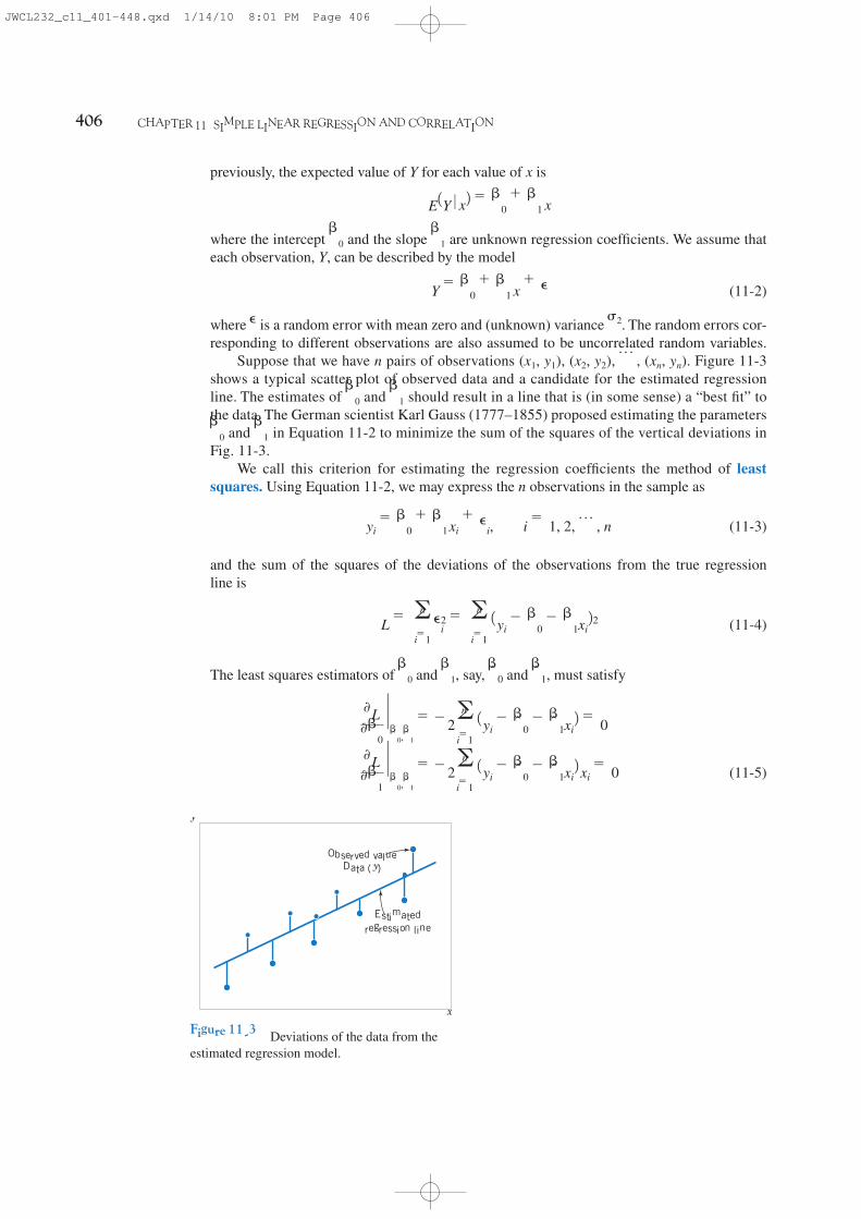
Suppose that we have n pairs of observations (x1, y1), (x2, y2), p , (xn, yn). Figure 11-3shows a typical scatter plot of observed data and a candidate for the estimated regressionline. The estimates of 0 and 1 should result in a line that is (in some sense) a “best fit” tothe data. The German scientist Karl Gauss (1777–1855) proposed estimating the parameters0 and 1 in Equation 11-2 to minimize the sum of the squares of the vertical deviations inFig. 11-3.
We call this criterion for estimating the regression coefficients the method of leastsquares. Using Equation 11-2, we may express the n observations in the sample as
(11-3)
and the sum of the squares of the deviations of the observations from the true regression line is
(11-4)
The least squares estimators of 0 and 1, say, and must satisfy
(11-5)ѨLѨ1`0,1
ϭ Ϫ2 an
iϭ11yi Ϫ 0 Ϫ 1xi2 xi ϭ 0
ѨLѨ0`0,1
ϭ Ϫ2 an
iϭ11yi Ϫ 0 Ϫ 1xi2 ϭ 0
1,0
L ϭ an
iϭ1⑀2
i ϭ an
iϭ11yi Ϫ 0 Ϫ 1xi22
yi ϭ 0 ϩ 1xi ϩ ⑀i, i ϭ 1, 2, p , n
Y ϭ 0 ϩ 1 x ϩ ⑀
E1Y 0 x2 ϭ 0 ϩ 1 x
x
y
Observed value
Data (y)
Estimated
regression line
Figure 11-3 Deviations of the data from theestimated regression model.
JWCL232_c11_401-448.qxd 1/14/10 8:01 PM Page 406

11-2 SIMPLE LINEAR REGRESSION 407
Simplifying these two equations yields
(11-6)
Equations 11-6 are called the least squares normal equations. The solution to the normalequations results in the least squares estimators and 1.0
0 an
iϭ1xi ϩ 1 a
n
iϭ1x i
2 ϭ an
iϭ1yixi
n0 ϩ 1 an
iϭ1xi ϭ a
n
iϭ1yi
The least squares estimates of the intercept and slope in the simple linear regressionmodel are
(11-7)
(11-8)
where y ϭ 11րn2 g niϭ1 yi and x ϭ 11րn2 g n
iϭ1 xi.
1 ϭa
n
iϭ1yi
xi Ϫ
aaniϭ1
yibaaniϭ1
xibn
an
iϭ1x2
i Ϫ
aaniϭ1
xib2
n
0 ϭ y Ϫ 1x
Least SquaresEstimates
The fitted or estimated regression line is therefore
(11-9)
Note that each pair of observations satisfies the relationship
where ei ϭ yi Ϫ is called the residual. The residual describes the error in the fit of themodel to the ith observation yi. Later in this chapter we will use the residuals to provideinformation about the adequacy of the fitted model.
Notationally, it is occasionally convenient to give special symbols to the numerator anddenominator of Equation 11-8. Given data (x1, y1), (x2, y2), p , (xn, yn), let
(11-10)
and
(11-11)Sxy ϭ an
iϭ11yi Ϫ y2 1xi Ϫ x2 ϭ a
n
iϭ1xiyi Ϫ
aaniϭ1
xib aaniϭ1
yibn
Sxx ϭ an
iϭ11xi Ϫ x22 ϭ a
n
iϭ1x2
i Ϫ
aaniϭ1
xib2
n
yi
yi ϭ 0 ϩ 1xi ϩ ei, i ϭ 1, 2, p , n
y ϭ 0 ϩ 1x
JWCL232_c11_401-448.qxd 1/15/10 4:53 PM Page 407

408 CHAPTER 11 SIMPLE LINEAR REGRESSION AND CORRELATION
Computer software programs are widely used in regression modeling. These programstypically carry more decimal places in the calculations. Table 11-2 shows a portion of theoutput from Minitab for this problem. The estimates and are highlighted. In subse-quent sections we will provide explanations for the information provided in this computeroutput.
10
EXAMPLE 11-1 Oxygen PurityWe will fit a simple linear regression model to the oxygenpurity data in Table 11-1. The following quantities may becomputed:
Sxx ϭ a20
iϭ1x i
2 Ϫ
aa20
iϭ1xib2
20ϭ 29.2892 Ϫ
123.922220
a20
iϭ1xi yi ϭ 2,214.6566
a20
iϭ1yi
2 ϭ 170,044.5321 a20
iϭ1xi
2 ϭ 29.2892
x ϭ 1.1960 y ϭ 92.1605
n ϭ 20 a20
iϭ1xi ϭ 23.92 a
20
iϭ1yi ϭ 1,843.21
Therefore, the least squares estimates of the slope and inter-cept are
and
The fitted simple linear regression model (with the coefficientsreported to three decimal places) is
This model is plotted in Fig. 11-4, along with the sample data.Practical Interpretation: Using the regression model, we
would predict oxygen purity of ϭ 89.23% when thehydrocarbon level is x ϭ 1.00%. The purity 89.23% may beinterpreted as an estimate of the true population mean puritywhen x ϭ 1.00%, or as an estimate of a new observationwhen x = 1.00%. These estimates are, of course, subject toerror; that is, it is unlikely that a future observation on puritywould be exactly 89.23% when the hydrocarbon level is1.00%. In subsequent sections we will see how to use confi-dence intervals and prediction intervals to describe the errorin estimation from a regression model.
y
y ϭ 74.283 ϩ 14.947x
0 ϭ y Ϫ 1x ϭ 92.1605 Ϫ 114.9474821.196 ϭ 74.28331
1 ϭSxy
Sxxϭ
10.177440.68088
ϭ 14.94748
90
87
93
96
99
102
0.87 1.07 1.27 1.47 1.67
Hydrocarbon level (%)
Oxy
gen p
uri
ty y
(%
)
x
Figure 11-4 Scatterplot of oxygen purity y versushydrocarbon level xand regression model
.y ϭ 74.283 ϩ 14.947x
ϭ 0.68088
and
ϭ 2,214.6566 Ϫ123.922 11,843.212
20ϭ 10.17744
Sxy ϭ a20
iϭ1xiyi Ϫ
aa20
iϭ1xib aa20
iϭ1yib
20
JWCL232_c11_401-448.qxd 1/14/10 8:02 PM Page 408

11-2 SIMPLE LINEAR REGRESSION 409
Table 11-2 Minitab Output for the Oxygen Purity Data in Example 11-1
Regression Analysis
The regression equation is
Purity ϭ 74.3 ϩ 14.9 HC Level
Predictor Coef SE Coef T PConstant 74.283 1.593 46.62 0.000HC Level 14.947 1.317 11.35 0.000
S ϭ 1.087 R-Sq ϭ 87.7% R-Sq (adj) ϭ 87.1%
Analysis of Variance
Source DF SS MS F PRegression 1 152.13 152.13 128.86 0.000Residual Error 18 21.25 SSE 1.18Total 19 173.38
Predicted Values for New Observations
New Obs Fit SE Fit 95.0% CI 95.0% PI1 89.231 0.354 (88.486, 89.975) (86.830, 91.632)
Values of Predictors for New Observations
New Obs HC Level1 1.00
2
1
0
Estimating 2
There is actually another unknown parameter in our regression model, 2 (the variance of theerror term ⑀). The residuals are used to obtain an estimate of 2. The sum ofsquares of the residuals, often called the error sum of squares, is
(11-12)
We can show that the expected value of the error sum of squares is E(SSE) ϭ (n Ϫ 2)2.Therefore an unbiased estimator of 2 is
SSE ϭ an
iϭ1ei
2 ϭ an
iϭ11 yi Ϫ yi22
ei ϭ yi Ϫ yi
(11-14)SSE ϭ SST Ϫ 1Sxy
(11-13)2 ϭSSE
n Ϫ 2
Estimator of Variance
Computing SSE using Equation 11-12 would be fairly tedious. A more convenient computingformula can be obtained by substituting into Equation 11-12 and simplifying.The resulting computing formula is
yi ϭ 0 ϩ 1xi
JWCL232_c11_401-448.qxd 1/14/10 8:02 PM Page 409

410 CHAPTER 11 SIMPLE LINEAR REGRESSION AND CORRELATION
where is the total sum of squares of the responsevariable y. Formulas such as this are presented in Section 11-4. The error sum of squares andthe estimate of 2 for the oxygen purity data, are highlighted in the Minitab outputin Table 11-2.
2 ϭ 1.18,
SST ϭ g niϭ1 1 yi Ϫ y 22 ϭ g n
iϭ1 yi2 Ϫ nyϪ2
EXERCISES FOR SECTION 11-2
11-1. An article in Concrete Research [“Near SurfaceCharacteristics of Concrete: Intrinsic Permeability” (Vol. 41,1989)] presented data on compressive strength x and intrinsic per-meability y of various concrete mixes and cures. Summary quan-tities are n ϭ 14, gyi ϭ 572, g ϭ 23,530, g xi ϭ 43, ϭg xi
2y2i
(e) Given that yards, find the fitted value of y and thecorresponding residual.
x ϭ 7.21
Yards per RatingPlayer Team Attempt Points
Philip Rivers SD 8.39 105.5Chad Pennington MIA 7.67 97.4Kurt Warner ARI 7.66 96.9Drew Brees NO 7.98 96.2Peyton Manning IND 7.21 95Aaron Rodgers GB 7.53 93.8Matt Schaub HOU 8.01 92.7Tony Romo DAL 7.66 91.4Jeff Garcia TB 7.21 90.2Matt Cassel NE 7.16 89.4Matt Ryan ATL 7.93 87.7Shaun Hill SF 7.10 87.5Seneca Wallace SEA 6.33 87Eli Manning NYG 6.76 86.4Donovan McNabb PHI 6.86 86.4Jay Cutler DEN 7.35 86Trent Edwards BUF 7.22 85.4Jake Delhomme CAR 7.94 84.7Jason Campbell WAS 6.41 84.3David Garrard JAC 6.77 81.7Brett Favre NYJ 6.65 81Joe Flacco BAL 6.94 80.3Kerry Collins TEN 6.45 80.2Ben Roethlisberger PIT 7.04 80.1Kyle Orton CHI 6.39 79.6JaMarcus Russell OAK 6.58 77.1Tyler Thigpen KC 6.21 76Gus Freotte MIN 7.17 73.7Dan Orlovsky DET 6.34 72.6Marc Bulger STL 6.18 71.4Ryan Fitzpatrick CIN 5.12 70Derek Anderson CLE 5.71 66.5
157.42, and g xiyi ϭ 1697.80. Assume that the two variablesare related according to the simple linear regression model.(a) Calculate the least squares estimates of the slope and intercept.
Estimate 2. Graph the regression line.(b) Use the equation of the fitted line to predict what perme-
ability would be observed when the compressive strengthis x ϭ 4.3.
(c) Give a point estimate of the mean permeability whencompressive strength is x ϭ 3.7.
(d) Suppose that the observed value of permeability at x ϭ
3.7 is y ϭ 46.1. Calculate the value of the correspondingresidual.
11-2. Regression methods were used to analyze the datafrom a study investigating the relationship between roadwaysurface temperature (x) and pavement deflection ( y). Summaryquantities were n ϭ 20, g yi ϭ 12.75, ϭ 8.86, g xi ϭg yi
2
1478, ϭ 143,215.8, and g xiyi ϭ 1083.67.(a) Calculate the least squares estimates of the slope and in-
tercept. Graph the regression line. Estimate 2.(b) Use the equation of the fitted line to predict what pave-
ment deflection would be observed when the surfacetemperature is 85ЊF.
(c) What is the mean pavement deflection when the surfacetemperature is 90ЊF?
(d) What change in mean pavement deflection would be ex-pected for a 1ЊF change in surface temperature?
11-3. The following table presents data on the ratings of quar-terbacks for the 2008 National Football League season (source:The Sports Network). It is suspected that the rating (y) is relatedto the average number of yards gained per pass attempt (x).(a) Calculate the least squares estimates of the slope and
intercept. What is the estimate of ? Graph the regres-sion model.
(b) Find an estimate of the mean rating if a quarterbackaverages 7.5 yards per attempt.
(c) What change in the mean rating is associated with adecrease of one yard per attempt?
(d) To increase the mean rating by 10 points, how much in-crease in the average yards per attempt must be generated?
2
gx2i
JWCL232_c11_401-448.qxd 1/15/10 4:53 PM Page 410

11-2 SIMPLE LINEAR REGRESSION 411
11-4. An article in Technometrics by S. C. Narula and J. F.Wellington [“Prediction, Linear Regression, and a MinimumSum of Relative Errors” (Vol. 19, 1977)] presents data on theselling price and annual taxes for 24 houses. The data areshown in the following table.
TaxesSale (Local, School),
Price/1000 County)/1000
25.9 4.917629.5 5.020827.9 4.542925.9 4.557329.9 5.059729.9 3.891030.9 5.898028.9 5.603935.9 5.828231.5 5.300331.0 6.271230.9 5.9592
TaxesSale (Local, School),
Price/1000 County)/1000
30.0 5.050036.9 8.246441.9 6.696940.5 7.784143.9 9.038437.5 5.989437.9 7.542244.5 8.795137.9 6.083138.9 8.360736.9 8.140045.8 9.1416
(a) Assuming that a simple linear regression model isappropriate, obtain the least squares fit relating sellingprice to taxes paid. What is the estimate of 2?
(b) Find the mean selling price given that the taxes paid arex ϭ 7.50.
(c) Calculate the fitted value of y corresponding to x ϭ
5.8980. Find the corresponding residual.(d) Calculate the fitted for each value of xi used to fit the
model. Then construct a graph of versus the correspon-ding observed value yi and comment on what this plotwould look like if the relationship between y and x was adeterministic (no random error) straight line. Does theplot actually obtained indicate that taxes paid is aneffective regressor variable in predicting selling price?
11-5. The number of pounds of steam used per month by achemical plant is thought to be related to the average ambienttemperature (inЊ F) for that month. The past year’s usage andtemperature are shown in the following table:
yi
yi
Month Temp. Usage/1000
Jan. 21 185.79Feb. 24 214.47Mar. 32 288.03Apr. 47 424.84May 50 454.58June 59 539.03
Month Temp. Usage/1000
July 68 621.55Aug. 74 675.06Sept. 62 562.03Oct. 50 452.93Nov. 41 369.95Dec. 30 273.98
(a) Assuming that a simple linear regression model is appro-priate, fit the regression model relating steam usage (y) tothe average temperature (x). What is the estimate of 2?Graph the regression line.
(b) What is the estimate of expected steam usage when theaverage temperature is 55ЊF?
(c) What change in mean steam usage is expected when themonthly average temperature changes by 1ЊF?
(d) Suppose the monthly average temperature is 47ЊF. Calculatethe fitted value of y and the corresponding residual.
11-6. The following table presents the highway gasolinemileage performance and engine displacement for Daimler-Chrysler vehicles for model year 2005 (source: U.S. Environ-mental Protection Agency).(a) Fit a simple linear model relating highway miles per gal-
lon ( y) to engine displacement (x) in cubic inches usingleast squares.
(b) Find an estimate of the mean highway gasoline mileageperformance for a car with 150 cubic inches enginedisplacement.
(c) Obtain the fitted value of y and the corresponding residualfor a car, the Neon, with an engine displacement of 122cubic inches.
Engine Displacement MPG
Carline (in3) (highway)
300C/SRT-8 215 30.8CARAVAN 2WD 201 32.5CROSSFIRE ROADSTER 196 35.4DAKOTA PICKUP 2WD 226 28.1DAKOTA PICKUP 4WD 226 24.4DURANGO 2WD 348 24.1GRAND CHEROKEE 2WD 226 28.5GRAND CHEROKEE 4WD 348 24.2LIBERTY/CHEROKEE 2WD 148 32.8LIBERTY/CHEROKEE 4WD 226 28NEON/SRT-4/SX 2.0 122 41.3PACIFICA 2WD 215 30.0PACIFICA AWD 215 28.2PT CRUISER 148 34.1RAM 1500 PICKUP 2WD 500 18.7RAM 1500 PICKUP 4WD 348 20.3SEBRING 4-DR 165 35.1STRATUS 4-DR 148 37.9TOWN & COUNTRY 2WD 148 33.8VIPER CONVERTIBLE 500 25.9WRANGLER/TJ 4WD 148 26.4
JWCL232_c11_401-448.qxd 1/14/10 8:02 PM Page 411

412 CHAPTER 11 SIMPLE LINEAR REGRESSION AND CORRELATION
11-7. An article in the Tappi Journal (March, 1986)presented data on green liquor Na2S concentration (in gramsper liter) and paper machine production (in tons per day). Thedata (read from a graph) are shown as follows:
y 40 42 49 46 44 48
x 825 830 890 895 890 910
y 46 43 53 52 54 57 58
x 915 960 990 1010 1012 1030 1050
(a) Fit a simple linear regression model with y ϭ green liquorNa2S concentration and x ϭ production. Find an estimateof 2. Draw a scatter diagram of the data and the resultingleast squares fitted model.
(b) Find the fitted value of y corresponding to x ϭ 910 andthe associated residual.
(c) Find the mean green liquor Na2S concentration when theproduction rate is 950 tons per day.
11-8. An article in the Journal of Sound and Vibration(Vol. 151, 1991, pp. 383–394) described a study investigatingthe relationship between noise exposure and hypertension.The following data are representative of those reported in thearticle.
y 1 0 1 2 5 1 4 6 2 3
x 60 63 65 70 70 70 80 90 80 80
y 5 4 6 8 4 5 7 9 7 6
x 85 89 90 90 90 90 94 100 100 100
(a) Draw a scatter diagram of y (blood pressure rise inmillimeters of mercury) versus x (sound pressure level indecibels). Does a simple linear regression model seemreasonable in this situation?
(b) Fit the simple linear regression model using least squares.Find an estimate of 2.
(c) Find the predicted mean rise in blood pressure levelassociated with a sound pressure level of 85 decibels.
11-9. An article in Wear (Vol. 152, 1992, pp. 171–181) pres-ents data on the fretting wear of mild steel and oil viscosity.Representative data follow, with x ϭ oil viscosity and y ϭ wearvolume ( cubic millimeters).10Ϫ4
y 110 113 75 94
x 35.5 43.0 40.5 33.0
y 240 181 193 155 172
x 1.6 9.4 15.5 20.0 22.0
(a) Construct a scatter plot of the data. Does a simple linearregression model appear to be plausible?
(b) Fit the simple linear regression model using least squares.Find an estimate of 2.
(c) Predict fretting wear when viscosity x ϭ 30.(d) Obtain the fitted value of y when x ϭ 22.0 and calculate
the corresponding residual.
11-10. An article in the Journal of EnvironmentalEngineering (Vol. 115, No. 3, 1989, pp. 608–619) reported theresults of a study on the occurrence of sodium and chloride insurface streams in central Rhode Island. The following dataare chloride concentration y (in milligrams per liter) androadway area in the watershed x (in percentage).
y 4.4 6.6 9.7 10.6 10.8 10.9
x 0.19 0.15 0.57 0.70 0.67 0.63
y 11.8 12.1 14.3 14.7 15.0 17.3
x 0.47 0.70 0.60 0.78 0.81 0.78
y 19.2 23.1 27.4 27.7 31.8 39.5
x 0.69 1.30 1.05 1.06 1.74 1.62
(a) Draw a scatter diagram of the data. Does a simple linearregression model seem appropriate here?
(b) Fit the simple linear regression model using the method ofleast squares. Find an estimate of 2.
(c) Estimate the mean chloride concentration for a watershedthat has 1% roadway area.
(d) Find the fitted value corresponding to x ϭ 0.47 and theassociated residual.
11-11. A rocket motor is manufactured by bonding togethertwo types of propellants, an igniter and a sustainer. The shearstrength of the bond y is thought to be a linear function of theage of the propellant x when the motor is cast. Twenty obser-vations are shown in the following table.(a) Draw a scatter diagram of the data. Does the straight-line
regression model seem to be plausible?(b) Find the least squares estimates of the slope and inter-
cept in the simple linear regression model. Find anestimate of 2.
(c) Estimate the mean shear strength of a motor made frompropellant that is 20 weeks old.
(d) Obtain the fitted values that correspond to each observedvalue yi. Plot versus yi and comment on what this plotwould look like if the linear relationship between shearstrength and age were perfectly deterministic (no error).Does this plot indicate that age is a reasonable choice ofregressor variable in this model?
yi
yi
JWCL232_c11_401-448.qxd 1/14/10 8:02 PM Page 412

11-2 SIMPLE LINEAR REGRESSION 413
11-12. An article in the Journal of the American CeramicSociety [“Rapid Hot-Pressing of Ultrafine PSZ Powders”(1991, Vol. 74, pp. 1547–1553)] considered the microstructureof the ultrafine powder of partially stabilized zirconia as afunction of temperature. The data are shown below:
x ϭ Temperature (ЊC): 1100 1200 1300 1100 15001200 1300
y ϭ Porosity (%): 30.8 19.2 6.0 13.5 11.47.7 3.6
(a) Fit the simple linear regression model using the method ofleast squares. Find an estimate of .2
Observation Strength y Age xNumber (psi) (weeks)
1 2158.70 15.502 1678.15 23.753 2316.00 8.004 2061.30 17.005 2207.50 5.006 1708.30 19.007 1784.70 24.008 2575.00 2.509 2357.90 7.50
10 2277.70 11.0011 2165.20 13.0012 2399.55 3.7513 1779.80 25.0014 2336.75 9.7515 1765.30 22.0016 2053.50 18.0017 2414.40 6.0018 2200.50 12.5019 2654.20 2.0020 1753.70 21.50
conducted over a period of time in days. The resulting data areshown below:
Time (days): 1 2 4 6 8 10 12 14 1618 20
BOD (mg/liter): 0.6 0.7 1.5 1.9 2.1 2.6 2.9 3.7 3.53.7 3.8
(a) Assuming that a simple linear regression model is appro-priate, fit the regression model relating BOD (y) to thetime (x). What is the estimate of ?
(b) What is the estimate of expected BOD level when the timeis 15 days?
(c) What change in mean BOD is expected when the timechanges by three days?
(d) Suppose the time used is six days. Calculate the fittedvalue of y and the corresponding residual.
(e) Calculate the fitted for each value of xi used to fit themodel. Then construct a graph of versus the correspon-ding observed values yi and comment on what this plotwould look like if the relationship between y and x was adeterministic (no random error) straight line. Does theplot actually obtained indicate that time is an effectiveregressor variable in predicting BOD?
11-14. An article in Wood Science and Technology [“Creepin Chipboard, Part 3: Initial Assessment of the Influence ofMoisture Content and Level of Stressing on Rate of Creepand Time to Failure” (1981, Vol. 15, pp. 125–144)] studiedthe deflection (mm) of particleboard from stress levels of rel-ative humidity. Assume that the two variables are related ac-cording to the simple linear regression model. The data areshown below:
x ϭ Stress level (%): 54 54 61 61 68y ϭ Deflection (mm): 16.473 18.693 14.305 15.121 13.505
x ϭ Stress level (%): 68 75 75 75y ϭ Deflection (mm): 11.640 11.168 12.534 11.224
(a) Calculate the least square estimates of the slope and inter-cept. What is the estimate of ? Graph the regressionmodel and the data.
(b) Find the estimate of the mean deflection if the stress levelcan be limited to 65%.
(c) Estimate the change in the mean deflection associatedwith a 5% increment in stress level.
(d) To decrease the mean deflection by one millimeter, howmuch increase in stress level must be generated?
(e) Given that the stress level is 68%, find the fitted value ofdeflection and the corresponding residual.
11-15. In an article in Statistics and Computing [“AnIterative Monte Carlo Method for Nonconjugate BayesianAnalysis” (1991, pp. 119–128)] Carlin and Gelfandinvestigated the age (x) and length (y) of 27 captured dugongs(sea cows).
2
yi
yi
2
(b) Estimate the mean porosity for a temperature of 1400ЊC.(c) Find the fitted value corresponding to and the
associated residual.(d) Draw a scatter diagram of the data. Does a simple linear
regression model seem appropriate here? Explain.11-13. An article in the Journal of the EnvironmentalEngineering Division [“Least Squares Estimates of BODParameters” (1980, Vol. 106, pp. 1197–1202)] took a samplefrom the Holston River below Kingport, Tennessee, duringAugust 1977. The biochemical oxygen demand (BOD) test is
y ϭ 11.4
JWCL232_c11_401-448.qxd 1/14/10 8:02 PM Page 413

414 CHAPTER 11 SIMPLE LINEAR REGRESSION AND CORRELATION
x ϭ 1.0, 1.5, 1.5, 1.5, 2.5, 4.0, 5.0, 5.0, 7.0, 8.0, 8.5, 9.0, 9.5,9.5, 10.0, 12.0, 12.0, 13.0, 13.0, 14.5, 15.5, 15.5, 16.5,17.0, 22.5, 29.0, 31.5
y ϭ 1.80, 1.85, 1.87, 1.77, 2.02, 2.27, 2.15, 2.26, 2.47, 2.19,2.26, 2.40, 2.39, 2.41, 2.50, 2.32, 2.32, 2.43, 2.47, 2.56,2.65, 2.47, 2.64, 2.56, 2.70, 2.72, 2.57
(a) Find the least squares estimates of the slope and the inter-cept in the simple linear regression model. Find an esti-mate of .
(b) Estimate the mean length of dugongs at age 11.(c) Obtain the fitted values that correspond to each ob-
served value yi. Plot versus yi, and comment on whatthis plot would look like if the linear relationship betweenlength and age were perfectly deterministic (no error).Does this plot indicate that age is a reasonable choice ofregressor variable in this model?
11-16. Consider the regression model developed in Ex-ercise 11-2.(a) Suppose that temperature is measured in ЊC rather than ЊF.
Write the new regression model.(b) What change in expected pavement deflection is associ-
ated with a 1ЊC change in surface temperature?
11-17. Consider the regression model developed in Exercise11-6. Suppose that engine displacement is measured in cubiccentimeters instead of cubic inches.
yi
yi
2
(a) Write the new regression model.(b) What change in gasoline mileage is associated with a
1 cm3 change is engine displacement?
11-18. Show that in a simple linear regression modelthe point ( ) lies exactly on the least squares regression line.x, y
( ) points. Use the two plots to intuitivelyexplain how the two models, Y ϭ 0 ϩ 1x ϩ ⑀ and
, are related.(b) Find the least squares estimates of and in the model
. How do they relate to the leastsquares estimates and ?
11-20. Suppose we wish to fit a regression model for whichthe true regression line passes through the point (0, 0). The ap-propriate model is Y ϭ x ϩ ⑀. Assume that we have n pairsof data (x1, y1), (x2, y2), p , (xn, yn). (a) Find the least squares estimate of .(b) Fit the model Y ϭ x ϩ ⑀ to the chloride concentration-
roadway area data in Exercise 11-10. Plot the fittedmodel on a scatter diagram of the data and comment onthe appropriateness of the model.
10
Y ϭ *0 ϩ *1z ϩ ⑀
*1*0Y ϭ *0 ϩ *1z ϩ ⑀
zi ϭ xi Ϫ x, yi
11-3 PROPERTIES OF THE LEAST SQUARES ESTIMATORS
The statistical properties of the least squares estimators and may be easily described.Recall that we have assumed that the error term ⑀ in the model Y ϭ 0 ϩ 1x ϩ ⑀ is a randomvariable with mean zero and variance 2. Since the values of x are fixed, Y is a random vari-able with mean ϭ 0 ϩ 1x and variance 2. Therefore, the values of and dependon the observed y’s; thus, the least squares estimators of the regression coefficients may beviewed as random variables. We will investigate the bias and variance properties of the leastsquares estimators and .
Consider first . Because is a linear combination of the observations Yi, we can useproperties of expectation to show that the expected value of is
(11-15)
Thus, is an unbiased estimator of the true slope 1.Now consider the variance of . Since we have assumed that V(⑀i) ϭ 2, it follows that
V(Yi) ϭ 2. Because is a linear combination of the observations Yi, the results inSection 5-5 can be applied to show that
(11-16)V112 ϭ2
Sxx
1
1
1
E112 ϭ 1
1
11
10
10Y 0 x10
11-19. Consider the simple linear regression model Y ϭ 0 ϩ
1x ϩ ⑀. Suppose that the analyst wants to use z ϭ x Ϫ asthe regressor variable.(a) Using the data in Exercise 11-11, construct one scatter
plot of the ( ) points and then another of thexi, yi
x
JWCL232_c11_401-448.qxd 1/14/10 8:02 PM Page 414

11-4 HYPOTHESIS TESTS IN SIMPLE LINEAR REGRESSION 415
For the intercept, we can show in a similar manner that
(11-17)
Thus, is an unbiased estimator of the intercept 0. The covariance of the random vari-ables and is not zero. It can be shown (see Exercise 11-98) that cov( ) ϭ
Ϫ2 .The estimate of 2 could be used in Equations 11-16 and 11-17 to provide estimates of
the variance of the slope and the intercept. We call the square roots of the resulting varianceestimators the estimated standard errors of the slope and intercept, respectively.
xրSxx
0, 110
0
E102 ϭ 0 and V102 ϭ 2 c 1n ϩx2
Sxxd
In simple linear regression the estimated standard error of the slope and the estimated standard error of the intercept are
respectively, where is computed from Equation 11-13.2
se112 ϭ B2
Sxx and se102 ϭ B2 c 1n ϩ
x2
Sxxd
EstimatedStandard
Errors
The Minitab computer output in Table 11-2 reports the estimated standard errors of the slopeand intercept under the column heading “SE coeff.”
11-4 HYPOTHESIS TESTS IN SIMPLE LINEAR REGRESSION
An important part of assessing the adequacy of a linear regression model is testing statisticalhypotheses about the model parameters and constructing certain confidence intervals. Hypothesistesting in simple linear regression is discussed in this section, and Section 11-5 presents methodsfor constructing confidence intervals. To test hypotheses about the slope and intercept of the re-gression model, we must make the additional assumption that the error component in themodel, ⑀, is normally distributed. Thus, the complete assumptions are that the errors are normallyand independently distributed with mean zero and variance 2, abbreviated NID(0, 2).
11-4.1 Use of t-Tests
Suppose we wish to test the hypothesis that the slope equals a constant, say, 1,0. The appro-priate hypotheses are
(11-18)
where we have assumed a two-sided alternative. Since the errors ⑀i are NID(0, 2), it followsdirectly that the observations Yi are NID(0 ϩ 1xi, 2). Now is a linear combination of 1
H1: 1 � 1,0
H0: 1 ϭ 1,0
JWCL232_c11_401-448.qxd 1/14/10 8:02 PM Page 415
416 CHAPTER 11 SIMPLE LINEAR REGRESSION AND CORRELATION
independent normal random variables, and consequently, is N(1, 2Sxx), using the bias1and variance properties of the slope discussed in Section 11-3. In addition, hasa chi-square distribution with n Ϫ 2 degrees of freedom, and is independent of . As aresult of those properties, the statistic
(11-19)
follows the t distribution with n Ϫ 2 degrees of freedom under H0: 1 ϭ 1,0. We would rejectH0: 1 ϭ 1,0 if
(11-20)
where t0 is computed from Equation 11-19. The denominator of Equation 11-19 is the standarderror of the slope, so we could write the test statistic as
A similar procedure can be used to test hypotheses about the intercept. To test
(11-21)
we would use the statistic
(11-22)
and reject the null hypothesis if the computed value of this test statistic, t0, is such that. Note that the denominator of the test statistic in Equation 11-22 is just the stan-
dard error of the intercept.A very important special case of the hypotheses of Equation 11-18 is
(11-23)
These hypotheses relate to the significance of regression. Failure to reject H0: 1 ϭ 0 isequivalent to concluding that there is no linear relationship between x and Y. This situation isillustrated in Fig. 11-5. Note that this may imply either that x is of little value in explaining thevariation in Y and that the best estimator of Y for any x is [Fig. 11-5(a)] or that the truey ϭ Y
H1: 1 � 0
H0: 1 ϭ 0
0 t0 0 Ͼ t␣ր2,nϪ2
T0 ϭ0 Ϫ 0,0
B2 c 1n ϩx2
Sxxd ϭ
0 Ϫ 0,0
se102H1: 0 � 0,0
H0: 0 ϭ 0,0
T0 ϭ1 Ϫ 1,0
se112
0 t0 0 Ͼ t␣ր2,nϪ2
T0 ϭ1 Ϫ 1,0
22րSxx
21
1n Ϫ 222ր2
Test Statistic
Test Statistic
relationship between x and Y is not linear [Fig. 11-5(b)]. Alternatively, if H0: 1 ϭ 0 is re-jected, this implies that x is of value in explaining the variability in Y (see Fig. 11-6). RejectingH0: 1 ϭ 0 could mean either that the straight-line model is adequate [Fig. 11-6(a)] or that,although there is a linear effect of x, better results could be obtained with the addition ofhigher order polynomial terms in x [Fig. 11-6(b)].
JWCL232_c11_401-448.qxd 1/14/10 8:02 PM Page 416

11-4 HYPOTHESIS TESTS IN SIMPLE LINEAR REGRESSION 417
x
y
(a)x
y
(b)
Figure 11-5 Thehypothesis H0: 1 ϭ 0is not rejected.
Figure 11-6 Thehypothesis H0: 1 ϭ 0is rejected.
x
y
(a)
x
y
(b)
EXAMPLE 11-2 Oxygen Purity Tests of Coefficients We will test for significance of regression using the model forthe oxygen purity data from Example 11-1. The hypotheses are
and we will use ␣ ϭ 0.01. From Example 11-1 and Table 11-2we have
so the t-statistic in Equation 10-20 becomes
t0 ϭ1
22րSxx
ϭ1
se112 ϭ14.947
21.18ր0.68088ϭ 11.35
1 ϭ 14.947 n ϭ 20, Sxx ϭ 0.68088, 2 ϭ 1.18
H1: 1 � 0H0: 1 ϭ 0
Practical Interpretation: Since the reference value of t ist0.005,18 ϭ 2.88, the value of the test statistic is very far into thecritical region, implying that H0: 1 ϭ 0 should be rejected.There is strong evidence to support this claim. The P-value forthis test is . This was obtained manuallywith a calculator.
Table 11-2 presents the Minitab output for this problem.Notice that the t-statistic value for the slope is computed as11.35 and that the reported P-value is P ϭ 0.000. Minitab alsoreports the t-statistic for testing the hypothesis H0: 0 ϭ 0.This statistic is computed from Equation 11-22, with 0,0 ϭ 0,as t0 ϭ 46.62. Clearly, then, the hypothesis that the intercept iszero is rejected.
P Ӎ 1.23 ϫ 10Ϫ9
11-4.2 Analysis of Variance Approach to Test Significance of Regression
A method called the analysis of variance can be used to test for significance of regression.The procedure partitions the total variability in the response variable into meaningful compo-nents as the basis for the test. The analysis of variance identity is as follows:
(11-24)an
iϭ11 yi Ϫ y 22 ϭ a
n
iϭ11 yi Ϫ y 22 ϩ a
n
iϭ11 yi Ϫ yi22Analysis of
VarianceIdentity
JWCL232_c11_401-448.qxd 1/15/10 5:37 PM Page 417

418 CHAPTER 11 SIMPLE LINEAR REGRESSION AND CORRELATION
(11-25)SST ϭ SSR ϩ SSE
(11-26)F0 ϭSSRր1
SSEր 1n Ϫ 22 ϭMSR
MSE
Test forSignificance of
Regression
The two components on the right-hand-side of Equation 11-24 measure, respectively, theamount of variability in yi accounted for by the regression line and the residual variation leftunexplained by the regression line. We usually call the error sum of squares and the regression sum of squares. Symbolically, Equation11-24 may be written as
SSR ϭ g niϭ1 1 yi Ϫ y 22 SSE ϭ g n
iϭ1 1yi Ϫ y i22
where SST ϭ gniϭ1 is the total corrected sum of squares of y. In Section 11-2 we1 yi Ϫ y22
noted that SSE ϭ SST Ϫ 1Sxy (see Equation 11-14), so since SST ϭ 1Sxy ϩ SSE, we note that theregression sum of squares in Equation 11-25 is SSR ϭ 1Sxy. The total sum of squares SST has n Ϫ 1 degrees of freedom, and SSR and SSE have 1 and n Ϫ 2 degrees of freedom, respectively.
ˆˆˆ
We may show that and that andSSEր2E 3SSEր 1n Ϫ 22 4 ϭ 2, E1SSR2 ϭ 2 ϩ 21Sxx
are independent chi-square random variables with n Ϫ 2 and 1 degrees of freedom, re-SSRր2
spectively. Thus, if the null hypothesis H0: 1 ϭ 0 is true, the statistic
follows the F1,nϪ2 distribution, and we would reject H0 if f0 Ͼ f␣,1,nϪ2. The quantities MSR ϭ
SSR1 and MSE ϭ SSE(n Ϫ 2) are called mean squares. In general, a mean square is alwayscomputed by dividing a sum of squares by its number of degrees of freedom. The test proce-dure is usually arranged in an analysis of variance table, such as Table 11-3.
Table 11-3 Analysis of Variance for Testing Significance of Regression
Source of Sum of Degrees of MeanVariation Squares Freedom Square F0
Regression 1 MSR MSRMSE
Error SSE ϭ SST Ϫ Sxy n Ϫ 2 MSE
Total SST n Ϫ 1
Note that MSE ϭ .2
1
SSR ϭ 1Sxy
EXAMPLE 11-3 Oxygen Purity ANOVAWe will use the analysis of variance approach to test for signifi-cance of regression using the oxygen purity data model fromExample 11-1. Recall that SST ϭ 173.38, Sxy ϭ
10.17744, and n ϭ 20. The regression sum of squares is
and the error sum of squares is
ϭ 21.25ϭ 173.38 Ϫ 152.13SSE ϭ SST Ϫ SSR
SSR ϭ 1Sxy ϭ 114.947210.17744 ϭ 152.13
1 ϭ 14.947,
The analysis of variance for testing H0: 1 ϭ 0 is sum-marized in the Minitab output in Table 11-2. The test statisticis f0 ϭ MSRMSE ϭ 152.131.18 ϭ 128.86, for which wefind that the P-value is P Ӎ 1.23 ϫ 10Ϫ9, so we conclude that1 is not zero.
There are frequently minor differences in terminologyamong computer packages. For example, sometimes the re-gression sum of squares is called the “model” sum of squares,and the error sum of squares is called the “residual” sum ofsquares.
JWCL232_c11_401-448.qxd 1/14/10 8:02 PM Page 418

11-4 HYPOTHESIS TESTS IN SIMPLE LINEAR REGRESSION 419
Note that the analysis of variance procedure for testing for significance of regression isequivalent to the t-test in Section 11-4.1. That is, either procedure will lead to the same conclusions.This is easy to demonstrate by starting with the t-test statistic in Equation 11-19 with 1,0 ϭ 0, say
(11-27)
Squaring both sides of Equation 11-27 and using the fact that results in
(11-28)
Note that T 20 in Equation 11-28 is identical to F0 in Equation 11-26. It is true, in general, that
the square of a t random variable with v degrees of freedom is an F random variable, with oneand v degrees of freedom in the numerator and denominator, respectively. Thus, the test usingT0 is equivalent to the test based on F0. Note, however, that the t-test is somewhat more flexiblein that it would allow testing against a one-sided alternative hypothesis, while the F-test isrestricted to a two-sided alternative.
T20 ϭ
21Sxx
MSEϭ
1Sxy
MSEϭ
MSR
MSE
2 ϭ MSE
T0 ϭ1
22րSxx
11-21. Consider the computer output below.
The regression equation isY ϭ 12.9 ϩ 2.34 x
Predictor Coef SE Coef T PConstant 12.857 1.032 ? ?X 2.3445 0.1150 ? ?
S ϭ 1.48111 RϪSq ϭ 98.1% RϪSq(adj) ϭ 97.9%
Analysis of Variance
Source DF SS MS F PRegression 1 912.43 912.43 ? ?Residual Error 8 17.55 ?Total 9 929.98
(a) Fill in the missing information. You may use bounds forthe P-values.
(b) Can you conclude that the model defines a useful linearrelationship?
(c) What is your estimate of 2?11-22. Consider the computer output below.
The regression equation isY = 26.8 ϩ 1.48 x
Predictor Coef SE Coef T PConstant 26.753 2.373 ? ?X 1.4756 0.1063 ? ?
S ϭ 2.70040 RϪSq ϭ 93.7% R-Sq (adj) ϭ 93.2%
Analysis of Variance
Source DF SS MS F PRegression 1 ? ? ? ?Residual Error ? 94.8 7.3Total 15 1500.0
(a) Fill in the missing information. You may use bounds forthe P-values.
(b) Can you conclude that the model defines a useful linearrelationship?
(c) What is your estimate of 2?
11-23. Consider the data from Exercise 11-1 on x ϭ
compressive strength and y ϭ intrinsic permeability of concrete.(a) Test for significance of regression using ␣ ϭ 0.05. Find
the P-value for this test. Can you conclude that the modelspecifies a useful linear relationship between these twovariables?
(b) Estimate 2 and the standard deviation of (c) What is the standard error of the intercept in this model?
11-24. Consider the data from Exercise 11-2 on x ϭ road-way surface temperature and y ϭ pavement deflection.(a) Test for significance of regression using ␣ ϭ 0.05. Find
the P-value for this test. What conclusions can you draw?(b) Estimate the standard errors of the slope and intercept.
11-25. Consider the National Football League data inExercise 11-3.(a) Test for significance of regression using . Find
the P-value for this test. What conclusions can you draw?(b) Estimate the standard errors of the slope and intercept.(c) Test versus with .
Would you agree with the statement that this is a test ofthe hypothesis that a one-yard increase in the averageyards per attempt results in a mean increase of 10 ratingpoints?
11-26. Consider the data from Exercise 11-4 on y ϭ salesprice and x ϭ taxes paid.(a) Test H0: 1 ϭ 0 using the t-test; use ␣ ϭ 0.05.(b) Test H0: 1 ϭ 0 using the analysis of variance with ␣ ϭ 0.05.
Discuss the relationship of this test to the test from part (a).
␣ ϭ 0.01H1: 1 � 10H0: 1 ϭ 10
␣ ϭ 0.01
1.
EXERCISES FOR SECTION 11-4
JWCL232_c11_401-448.qxd 1/14/10 8:02 PM Page 419

420 CHAPTER 11 SIMPLE LINEAR REGRESSION AND CORRELATION
(c) Estimate the standard errors of the slope and intercept.(d) Test the hypothesis that 0 ϭ 0.11-27. Consider the data from Exercise 11-5 on y ϭ steamusage and x ϭ average temperature.(a) Test for significance of regression using ␣ ϭ 0.01. What
is the P-value for this test? State the conclusions thatresult from this test.
(b) Estimate the standard errors of the slope and intercept.(c) Test the hypothesis H0: 1 ϭ 10 versus H1: 1 ϶ 10 using
␣ ϭ 0.01. Find the P-value for this test.(d) Test H0: 0 ϭ 0 versus H1: 0 ϶ 0 using ␣ ϭ 0.01. Find
the P-value for this test and draw conclusions.11-28. Consider the data from Exercise 11-6 on y ϭ highwaygasoline mileage and x ϭ engine displacement.(a) Test for significance of regression using ␣ ϭ 0.01. Find
the P-value for this test. What conclusions can youreach?
(b) Estimate the standard errors of the slope and intercept.(c) Test H0: 1 ϭ Ϫ0.05 versus H1: 1 Ͻ Ϫ0.05 using ␣ ϭ
0.01 and draw conclusions. What is the P-value for this test?(d) Test the hypothesis H0: 0 ϭ 0 versus H1: 0 ϶ 0 using
␣ ϭ 0.01. What is the P-value for this test?11-29. Consider the data from Exercise 11-7 on y ϭ greenliquor Na2S concentration and x ϭ production in a paper mill.(a) Test for significance of regression using ␣ ϭ 0.05. Find
the P-value for this test.(b) Estimate the standard errors of the slope and intercept.(c) Test H0: 0 ϭ 0 versus H1: 0 ϶ 0 using ␣ ϭ 0.05. What
is the P-value for this test?11-30. Consider the data from Exercise 11-8 on y ϭ bloodpressure rise and x ϭ sound pressure level.(a) Test for significance of regression using ␣ ϭ 0.05. What
is the P-value for this test?(b) Estimate the standard errors of the slope and intercept.(c) Test H0: 0 ϭ 0 versus H1: 0 ϶ 0 using ␣ ϭ 0.05. Find
the P-value for this test.11-31. Consider the data from Exercise 11-11, on y ϭ shearstrength of a propellant and x ϭ propellant age.(a) Test for significance of regression with ␣ ϭ 0.01. Find the
P-value for this test.(b) Estimate the standard errors of and (c) Test H0: 1 ϭ Ϫ30 versus H1: 1 ϶ Ϫ30 using ␣ ϭ 0.01.
What is the P-value for this test?(d) Test H0: 0 ϭ 0 versus H1: 0 ϶ 0 using ␣ ϭ 0.01. What
is the P-value for this test?(e) Test H0: 0 ϭ 2500 versus H1: 0 Ͼ 2500 using ␣ ϭ
0.01. What is the P-value for this test?11-32. Consider the data from Exercise 11-10 on y ϭ chlorideconcentration in surface streams and x ϭ roadway area.(a) Test the hypothesis H0: 1 ϭ 0 versus H1: 1 ϶ 0 using
the analysis of variance procedure with ␣ ϭ 0.01.(b) Find the P-value for the test in part (a).(c) Estimate the standard errors of and 0.1
1.0
(d) Test H0: 0 ϭ 0 versus H1: 0 ϶ 0 using ␣ ϭ 0.01. Whatconclusions can you draw? Does it seem that the modelmight be a better fit to the data if the intercept were removed?
11-33. Consider the data in Exercise 11-13 on and .
(a) Test for significance of regression using . Findthe P-value for this test. What conclusions can you draw?
(b) Estimate the standard errors of the slope and intercept.(c) Test the hypothesis that .11-34. Consider the data in Exercise 11-14 on and .(a) Test for significance of regression using . What
is the P-value for this test? State the conclusions that resultfrom this test.
(b) Does this model appear to be adequate?(c) Estimate the standard errors of the slope and intercept.11-35. An article in The Journal of Clinical Endocrinologyand Metabolism [“Simultaneous and Continuous 24-HourPlasma and Cerebrospinal Fluid Leptin Measurements:Dissociation of Concentrations in Central and PeripheralCompartments” (2004, Vol. 89, pp. 258–265)] studied thedemographics of simultaneous and continuous 24-hourplasma and cerebrospinal fluid leptin measurements. The datafollow:
y ϭ BMI (kg/m2): 19.92 20.59 29.02 20.78 25.9720.39 23.29 17.27 35.24
x ϭ Age (yr): 45.5 34.6 40.6 32.9 28.2 30.152.1 33.3 47.0
(a) Test for significance of regression using . Find theP-value for this test. Can you conclude that the model speci-fies a useful linear relationship between these two variables?
(b) Estimate and the standard deviation of .(c) What is the standard error of the intercept in this model?11-36. Suppose that each value of xi is multiplied by a pos-itive constant a, and each value of yi is multiplied by anotherpositive constant b. Show that the t-statistic for testing H0: 1 ϭ 0 versus H1: 1 ϶ 0 is unchanged in value.11-37. The type II error probability for the t-test for H0: 1 ϭ 1,0 can be computed in a similar manner to the t-tests of Chapter 9. If the true value of 1 is œ
1, the valueis calculated and used as
the horizontal scale factor on the operating characteristic curvesfor the t-test (Appendix Charts VIIe through VIIh) and the typeII error probability is read from the vertical scale using the curvefor n Ϫ 2 degrees of freedom. Apply this procedure to the foot-ball data of Exercise 11-3, using ϭ 5.5 and œ
1 ϭ 12.5, wherethe hypotheses are H0: 1 ϭ 10 versus H1: 1 � 10.11-38. Consider the no-intercept model Y ϭ x ϩ ⑀
with the ⑀’s NID(0, 2). The estimate of 2 is s2 ϭ
gniϭ1 and V ϭ 2gn
iϭ1
(a) Devise a test statistic for H0:  ϭ 0 versus H1:  ϶ 0.(b) Apply the test in (a) to the model from Exercise 11-20.
x 2i .121 yi Ϫ xi22ր 1n Ϫ 12
d ϭ 01,0 Ϫ ¿1 0 ր 111n Ϫ 12րSxx
12
␣ ϭ 0.05
␣ ϭ 0.01x ϭ stress level
y ϭ deflection0 ϭ 0
␣ ϭ 0.01x ϭ timeoxygen demand
y ϭ
JWCL232_c11_401-448.qxd 1/14/10 8:02 PM Page 420
11-5 CONFIDENCE INTERVALS 421
11-5 CONFIDENCE INTERVALS
11-5.1 Confidence Intervals on the Slope and Intercept
In addition to point estimates of the slope and intercept, it is possible to obtain confidenceinterval estimates of these parameters. The width of these confidence intervals is a measure ofthe overall quality of the regression line. If the error terms, ⑀i, in the regression model arenormally and independently distributed,
are both distributed as t random variables with n Ϫ 2 degrees of freedom. This leads to thefollowing definition of 100(1 Ϫ ␣)% confidence intervals on the slope and intercept.
11 Ϫ 12ր22րSxx and 10 Ϫ 02րB2 c 1n ϩx2
Sxxd
Under the assumption that the observations are normally and independently distributed,a 100(1 Ϫ ␣)% confidence interval on the slope 1 in simple linear regression is
(11-29)
Similarly, a 100(1 Ϫ ␣)% confidence interval on the intercept 0 is
(11-30)Յ 0 Յ 0 ϩ t␣ր2,nϪ2B2 c 1n ϩx2
Sxxd
0 Ϫ t␣ր2,nϪ2 B2 c 1n ϩx2
Sxxd
1 Ϫ t␣ր2,nϪ2B2
SxxՅ 1 Յ 1 ϩ t␣ր2,nϪ2 B
2
Sxx
ConfidenceIntervals onParameters
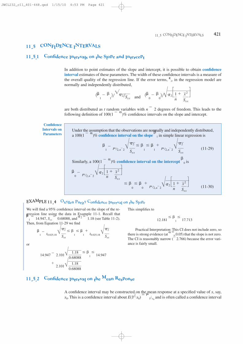
EXAMPLE 11-4 Oxygen Purity Confidence Interval on the SlopeWe will find a 95% confidence interval on the slope of the re-gression line using the data in Example 11-1. Recall that
Sxx ϭ 0.68088, and (see Table 11-2).Then, from Equation 11-29 we find
or
ϩ 2.101A1.18
0.68088
14.947 Ϫ 2.101A1.18
0.68088Յ 1 Յ 14.947
1 Ϫ t0.025,18 B2
SxxՅ 1 Յ 1 ϩ t0.025,18 B
2
Sxx
2 ϭ 1.181 ϭ 14.947,
This simplifies to
Practical Interpretation: This CI does not include zero, sothere is strong evidence (at ␣ ϭ 0.05) that the slope is not zero.The CI is reasonably narrow ( 2.766) because the error vari-ance is fairly small.
Ϯ
12.181 Յ 1 Յ 17.713
11-5.2 Confidence Interval on the Mean Response
A confidence interval may be constructed on the mean response at a specified value of x, say,x0. This is a confidence interval about E(Y x0) ϭ Y x0
and is often called a confidence interval
JWCL232_c11_401-448.qxd 1/15/10 4:53 PM Page 421
422 CHAPTER 11 SIMPLE LINEAR REGRESSION AND CORRELATION
about the regression line. Since E(Y x0) ϭ Y x0ϭ 0 ϩ 1x0, we may obtain a point estimate
of the mean of Y at x ϭ x0(Y x0) from the fitted model as
Now is an unbiased point estimator of Y x0, since and are unbiased estimators of
0 and 1. The variance of is
This last result follows from the fact that and cov The zerocovariance result is left as a mind-expanding exercise. Also, is normally distributed, because
1 and 0 are normally distributed, and if we use as an estimate of 2, it is easy to show that
has a t distribution with n Ϫ 2 degrees of freedom. This leads to the following confidenceinterval definition.
Y 0 x0Ϫ Y 0 x0
B2 c 1n ϩ1x0 Ϫ x 22
Sxxd
2
Y 0 x0
1Y, 12 ϭ 0.Y |x0ϭ y ϩ 11x0 Ϫ x2
V 1Y 0 x02 ϭ 2 c 1n ϩ
1x0 Ϫ x22Sxx
dY 0 x0
10Y 0 x0
Y 0 x0ϭ 0 ϩ 1x0
A 100(1 Ϫ ␣)% confidence interval about the mean response at the value of x ϭ x0, say , is given by
(11-31)
where is computed from the fitted regression model.Y 0 x0ϭ 0 ϩ 1x0
Յ Y 0 x0Յ Y 0 x0
ϩ t␣ր2,nϪ2B2 c 1n ϩ1x0 Ϫ x 22
Sxxd
Y 0x0Ϫ t␣ր2,nϪ2B2 c 1n ϩ
1x0 Ϫ x 22Sxx
dY 0 x0
ConfidenceInterval on the
Mean Response
Note that the width of the CI for is a function of the value specified for x0. The intervalwidth is a minimum for and widens as increases.0 x0 Ϫ x 0x0 ϭ x
Y 0 x0
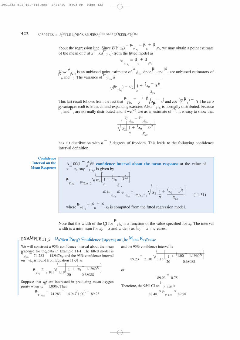
EXAMPLE 11-5 Oxygen Purity Confidence Interval on the Mean ResponseWe will construct a 95% confidence interval about the meanresponse for the data in Example 11-1. The fitted model is
and the 95% confidence intervalon is found from Equation 11-31 as
Suppose that we are interested in predicting mean oxygen purity when x0 ϭ 1.00%. Then
Y 0 x1.00ϭ 74.283 ϩ 14.94711.002 ϭ 89.23
Y 0 x0Ϯ 2.101B1.18 c 1
20ϩ1x0 Ϫ 1.196022
0.68088d
Y 0 x0
Y 0 x0ϭ 74.283 ϩ 14.947x0,
and the 95% confidence interval is
or
Therefore, the 95% CI on is
88.48 Յ Y 0 1.00 Յ 89.98
Y 0 1.00
89.23 Ϯ 0.75
89.23 Ϯ 2.101B1.18 c 120
ϩ11.00 Ϫ 1.196022
0.68088d
JWCL232_c11_401-448.qxd 1/14/10 8:03 PM Page 422

11-6 PREDICTION OF NEW OBSERVATIONS 423
This is a reasonable narrow CI.Minitab will also perform these calculations. Refer to
Table 11-2. The predicted value of y at x ϭ 1.00 is shownalong with the 95% CI on the mean of y at this level of x.
By repeating these calculations for several different val-ues for x0, we can obtain confidence limits for each correspon-ding value of . Figure 11-7 displays the scatter diagramY 0 x0
with the fitted model and the corresponding 95% confidencelimits plotted as the upper and lower lines. The 95% confi-dence level applies only to the interval obtained at one valueof x and not to the entire set of x-levels. Notice that the widthof the confidence interval on increases asincreases.
0 x0 Ϫ x 0Y 0 x0
90
87
93
96
99
102
0.87 1.07 1.27 1.47 1.67
Hydrocarbon level (%)
Oxy
gen p
uri
ty y
(%
)
x
Figure 11-7 Scatterdiagram of oxygen purity data fromExample 11-1 with fitted regression lineand 95 percent confidence limits on
.Y 0 x0
11-6 PREDICTION OF NEW OBSERVATIONS
An important application of a regression model is predicting new or future observations Ycorresponding to a specified level of the regressor variable x. If x0 is the value of the regressorvariable of interest,
(11-32)
is the point estimator of the new or future value of the response Y0.Now consider obtaining an interval estimate for this future observation Y0. This new
observation is independent of the observations used to develop the regression model.Therefore, the confidence interval for in Equation 11-31 is inappropriate, since it is basedonly on the data used to fit the regression model. The confidence interval about refers tothe true mean response at x ϭ x0 (that is, a population parameter), not to future observations.
Let Y0 be the future observation at x ϭ x0, and let given by Equation 11-32 be theestimator of Y0. Note that the error in prediction
is a normally distributed random variable with mean zero and variance
V 1ep2 ϭ V1Y0 Ϫ Y02 ϭ 2 c1 ϩ1n ϩ
1x0 Ϫ x 22Sxx
dep ϭ Y0 Ϫ Y0
Y0
Y 0 x0
Y 0 x0
Y0 ϭ 0 ϩ 1x0
JWCL232_c11_401-448.qxd 1/14/10 8:03 PM Page 423
because Y0 is independent of If we use to estimate 2, we can show that
has a t distribution with n Ϫ 2 degrees of freedom. From this we can develop the followingprediction interval definition.
Y0 Ϫ Y0
B2 c1 ϩ1n ϩ
1x0 Ϫ x 22Sxx
d2Y0.
424 CHAPTER 11 SIMPLE LINEAR REGRESSION AND CORRELATION
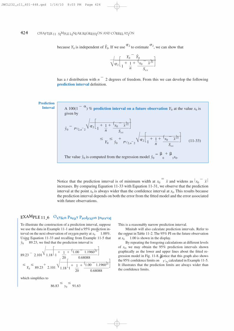
A 100(1 Ϫ ␣) % prediction interval on a future observation at the value x0 isgiven by
(11-33)
The value is computed from the regression model y0 ϭ 0 ϩ 1x0.y0
Յ Y0 Յ y0 ϩ t␣ր 2,nϪ2B2 c1 ϩ1n ϩ
1x0 Ϫ x 22Sxx
dy0 Ϫ t␣ր2,nϪ2B2 c1 ϩ
1n ϩ
1x0 Ϫ x 22Sxx
dY0
PredictionInterval
Notice that the prediction interval is of minimum width at and widens as increases. By comparing Equation 11-33 with Equation 11-31, we observe that the predictioninterval at the point x0 is always wider than the confidence interval at x0. This results becausethe prediction interval depends on both the error from the fitted model and the error associatedwith future observations.
0 x0 Ϫ x 0x0 ϭ x
EXAMPLE 11-6 Oxygen Purity Prediction IntervalTo illustrate the construction of a prediction interval, supposewe use the data in Example 11-1 and find a 95% prediction in-terval on the next observation of oxygen purity at x0 ϭ 1.00%.Using Equation 11-33 and recalling from Example 11-5 that
, we find that the prediction interval is
which simplifies to
86.83 Յ y0 Յ 91.63
B1.18 c1 ϩ1
20ϩ11.00 Ϫ1.196022
0.68088dՅ Y0 Յ 89.23 ϩ 2.101
89.23 Ϫ 2.101B1.18 c1 ϩ1
20ϩ11.00 Ϫ 1.196022
0.68088d
y0 ϭ 89.23
This is a reasonably narrow prediction interval.Minitab will also calculate prediction intervals. Refer to
the output in Table 11-2. The 95% PI on the future observationat x0 ϭ 1.00 is shown in the display.
By repeating the foregoing calculations at different levelsof x0, we may obtain the 95% prediction intervals showngraphically as the lower and upper lines about the fitted re-gression model in Fig. 11-8. Notice that this graph also showsthe 95% confidence limits on calculated in Example 11-5.It illustrates that the prediction limits are always wider thanthe confidence limits.
Y 0 x0
JWCL232_c11_401-448.qxd 1/14/10 8:03 PM Page 424

11-6 PREDICTION OF NEW OBSERVATIONS 425
Figure 11-8 Scatterdiagram of oxygenpurity data fromExample 11-1 withfitted regression line,95% prediction limits(outer lines) and 95%confidence limits on
.Y 0 x0
90
87
93
96
99
102
0.87 1.07 1.27 1.47 1.67
Hydrocarbon level (%)
x
Oxy
gen p
uri
ty y
(%
)
EXERCISES FOR SECTIONS 11-5 AND 11-6
11-39. Refer to the data in Exercise 11-1 on y ϭ intrinsicpermeability of concrete and x ϭ compressive strength. Finda 95% confidence interval on each of the following:(a) Slope (b) Intercept(c) Mean permeability when x ϭ 2.5(d) Find a 95% prediction interval on permeability when
x ϭ 2.5. Explain why this interval is wider than theinterval in part (c).
11-40. Exercise 11-2 presented data on roadway surfacetemperature x and pavement deflection y. Find a 99% confi-dence interval on each of the following:(a) Slope (b) Intercept(c) Mean deflection when temperature (d) Find a 99% prediction interval on pavement deflection
when the temperature is .11-41. Refer to the NFL quarterback ratings data inExercise 11-3. Find a 95% confidence interval on each of thefollowing:(a) Slope(b) Intercept(c) Mean rating when the average yards per attempt is 8.0(d) Find a 95% prediction interval on the rating when the
average yards per attempt is 8.0.11-42. Refer to the data on y ϭ house selling price and x ϭ taxes paid in Exercise 11-4. Find a 95% confidence inter-val on each of the following:(a) 1 (b) 0
(c) Mean selling price when the taxes paid are x ϭ 7.50(d) Compute the 95% prediction interval for selling price
when the taxes paid are x ϭ 7.50.11-43. Exercise 11-5 presented data on y ϭ steam usageand x ϭ monthly average temperature.
90ЊF
x ϭ 85ЊF
(a) Find a 99% confidence interval for 1.(b) Find a 99% confidence interval for 0.(c) Find a 95% confidence interval on mean steam usage
when the average temperature is .(d) Find a 95% prediction interval on steam usage when tem-
perature is . Explain why this interval is wider thanthe interval in part (c).
11-44. Exercise 11-6 presented gasoline mileage perfor-mance for 21 cars, along with information about the enginedisplacement. Find a 95% confidence interval on each of thefollowing:(a) Slope (b) Intercept(c) Mean highway gasoline mileage when the engine dis-
placement is x ϭ 150 in3
(d) Construct a 95% prediction interval on highway gasolinemileage when the engine displacement is x ϭ 150 in3.
11-45. Consider the data in Exercise 11-7 on y ϭ greenliquor Na2S concentration and x ϭ production in a papermill. Find a 99% confidence interval on each of the following:(a) 1 (b) 0
(c) Mean Na2S concentration when production x ϭ 910 tons �day
(d) Find a 99% prediction interval on Na2S concentrationwhen x ϭ 910 tons�day.
11-46. Exercise 11-8 presented data on y ϭ blood pressurerise and x ϭ sound pressure level. Find a 95% confidenceinterval on each of the following:(a) 1 (b) 0
(c) Mean blood pressure rise when the sound pressure level is85 decibels
(d) Find a 95% prediction interval on blood pressure risewhen the sound pressure level is 85 decibels.
55ЊF
55ЊF
JWCL232_c11_401-448.qxd 1/18/10 2:12 PM Page 425

426 CHAPTER 11 SIMPLE LINEAR REGRESSION AND CORRELATION
11-47. Refer to the data in Exercise 11-9 on y ϭ wearvolume of mild steel and x ϭ oil viscosity. Find a 95% confi-dence interval on each of the following:(a) Intercept (b) Slope(c) Mean wear when oil viscosity x ϭ 3011-48. Exercise 11-10 presented data on chloride concentra-tion y and roadway area x on watersheds in central RhodeIsland. Find a 99% confidence interval on each of the following:(a) 1 (b) 0
(c) Mean chloride concentration when roadway area x ϭ 1.0%(d) Find a 99% prediction interval on chloride concentration
when roadway area x ϭ 1.0%.11-49. Refer to the data in Exercise 11-11 on rocket motorshear strength y and propellant age x. Find a 95% confidenceinterval on each of the following:(a) Slope 1 (b) Intercept 0
(c) Mean shear strength when age x ϭ 20 weeks
(d) Find a 95% prediction interval on shear strength when agex ϭ 20 weeks.
11-50. Refer to the data in Exercise 11-12 on the mi-crostructure of zirconia. Find a 95% confidence interval oneach of the following:(a) Slope (b) Intercept(c) Mean length when (d) Find a 95% prediction interval on length when
Explain why this interval is wider than the interval inpart (c).
11-51. Refer to the data in Exercise 11-13 on oxygen de-mand. Find a 99% confidence interval on each of thefollowing:(a)(b)(c) Find a 95% confidence interval on mean BOD when the
time is 8 days.
0
1
x ϭ 1500.x ϭ 1500
11-7 ADEQUACY OF THE REGRESSION MODEL
Fitting a regression model requires several assumptions. Estimation of the model parametersrequires the assumption that the errors are uncorrelated random variables with mean zero andconstant variance. Tests of hypotheses and interval estimation require that the errors be nor-mally distributed. In addition, we assume that the order of the model is correct; that is, if wefit a simple linear regression model, we are assuming that the phenomenon actually behaves ina linear or first-order manner.
The analyst should always consider the validity of these assumptions to be doubtful andconduct analyses to examine the adequacy of the model that has been tentatively entertained.In this section we discuss methods useful in this respect.
11-7.1 Residual Analysis
The residuals from a regression model are where yi is an actualobservation and is the corresponding fitted value from the regression model. Analysis of theresiduals is frequently helpful in checking the assumption that the errors are approximatelynormally distributed with constant variance, and in determining whether additional terms inthe model would be useful.
As an approximate check of normality, the experimenter can construct a frequency his-togram of the residuals or a normal probability plot of residuals. Many computer programswill produce a normal probability plot of residuals, and since the sample sizes in regressionare often too small for a histogram to be meaningful, the normal probability plotting methodis preferred. It requires judgment to assess the abnormality of such plots. (Refer to the discus-sion of the “fat pencil” method in Section 6-6).
We may also standardize the residuals by computing , . Ifthe errors are normally distributed, approximately 95% of the standardized residuals shouldfall in the interval (Ϫ2, ϩ2). Residuals that are far outside this interval may indicate thepresence of an outlier, that is, an observation that is not typical of the rest of the data. Variousrules have been proposed for discarding outliers. However, outliers sometimes provide
i ϭ 1, 2, p , ndi ϭ eiր22
yi
ei ϭ yi Ϫ yi, i ϭ 1, 2, p , n,
JWCL232_c11_401-448.qxd 1/14/10 8:03 PM Page 426

11-7 ADEQUACY OF THE REGRESSION MODEL 427
important information about unusual circumstances of interest to experimenters and shouldnot be automatically discarded. For further discussion of outliers, see Montgomery, Peck, andVining (2006).
It is frequently helpful to plot the residuals (1) in time sequence (if known), (2), againstthe , and (3) against the independent variable x. These graphs will usually look like one ofthe four general patterns shown in Fig. 11-9. Pattern (a) in Fig. 11-9 represents the ideal situ-ation, while patterns (b), (c), and (d ) represent anomalies. If the residuals appear as in (b), thevariance of the observations may be increasing with time or with the magnitude of yi or xi. Datatransformation on the response y is often used to eliminate this problem. Widely used vari-ance-stabilizing transformations include the use of , ln y, or 1y as the response. SeeMontgomery, Peck, and Vining (2006) for more details regarding methods for selecting an ap-propriate transformation. Plots of residuals against and xi that look like (c) also indicate in-equality of variance. Residual plots that look like (d) indicate model inadequacy; that is,higher order terms should be added to the model, a transformation on the x-variable or the y-variable (or both) should be considered, or other regressors should be considered.
yi
1y
yi
Figure 11-9 Patterns for residual plots. (a) Satisfactory, (b) Funnel,(c) Double bow, (d) Nonlinear. [Adapted from Montgomery, Peck, andVining (2006).]
0
(a)
ei
0
(b)
ei
0
(c)
ei
0
(d)
ei
EXAMPLE 11-7 Oxygen Purity ResidualsThe regression model for the oxygen purity data in Example11-1 is ϭ 74.283 ϩ 14.947x. Table 11-4 presents the ob-served and predicted values of y at each value of x from thisdata set, along with the corresponding residual. These valueswere computed using Minitab and show the number of deci-mal places typical of computer output. A normal probability
yplot of the residuals is shown in Fig. 11-10. Since the residu-als fall approximately along a straight line in the figure, weconclude that there is no severe departure from normality. Theresiduals are also plotted against the predicted value in Fig.11-11 and against the hydrocarbon levels xi in Fig. 11-12.These plots do not indicate any serious model inadequacies.
yi
JWCL232_c11_401-448.qxd 1/14/10 8:03 PM Page 427

428 CHAPTER 11 SIMPLE LINEAR REGRESSION AND CORRELATION
Figure 11-10 Normal probability plot of residuals,Example 11-7.
Figure 11-11 Plot of residuals versus predicted oxygenpurity , Example 11-7.y
0.1
5
1
20
50
80
95
99
99.9
Cum
ula
tive
norm
al pro
babilit
y
0.1–1.9 –0.9 1.1 2.1
Residuals
89
–2
91 93 95 97
–1.5
–1
0
0.5
–0.5
1
1.5
2
2.5
–2.587 99
Predicted values, y
Resi
duals
Table 11-4 Oxygen Purity Data from Example 11-1, Predicted Values, and Residuals
Hydrocarbon Oxygen Predicted ResidualLevel, x Purity, y Value, e ϭ y Ϫ
1 0.99 90.01 89.081 0.9292 1.02 89.05 89.530 Ϫ0.4803 1.15 91.43 91.473 Ϫ0.0434 1.29 93.74 93.566 0.1745 1.46 96.73 96.107 0.6236 1.36 94.45 94.612 Ϫ0.1627 0.87 87.59 87.288 0.3028 1.23 91.77 92.669 Ϫ0.8999 1.55 99.42 97.452 1.968
10 1.40 93.65 95.210 Ϫ1.560
yyHydrocarbon Oxygen Predicted Residual
Level, x Purity, y Value, e ϭ y Ϫ
11 1.19 93.54 92.071 1.46912 1.15 92.52 91.473 1.04713 0.98 90.56 88.932 1.62814 1.01 89.54 89.380 0.16015 1.11 89.85 90.875 Ϫ1.02516 1.20 90.39 92.220 Ϫ1.83017 1.26 93.25 93.117 0.13318 1.32 93.41 94.014 Ϫ0.60419 1.43 94.98 95.658 Ϫ0.67820 0.95 87.33 88.483 Ϫ1.153
yy
The coefficient of determination is
(11-34)R2 ϭSSR
SSTϭ 1 Ϫ
SSE
SST
R2
11-7.2 Coefficient of Determination (R2)
A widely used measure for a regression model is the following ratio of sum of squares.
The coefficient is often used to judge the adequacy of a regression model. Subsequently, wewill see that in the case where X and Y are jointly distributed random variables, R2 is the squareof the correlation coefficient between X and Y. From the analysis of variance identity inEquations 11-24 and 11-25, 0 Յ R2 Յ 1. We often refer loosely to R2 as the amount of vari-ability in the data explained or accounted for by the regression model. For the oxygen purityregression model, we have R2 ϭ SSR SST ϭ 152.13 173.38 ϭ 0.877; that is, the model ac-counts for 87.7% of the variability in the data.
րր
JWCL232_c11_401-448.qxd 1/14/10 8:03 PM Page 428

11-7 ADEQUACY OF THE REGRESSION MODEL 429
Figure 11-12 Plot ofresiduals versus hydro-carbon level x,Example 11-8.
–0.9
–1,9
0.1
1.1
2.1
0.87 1.07 1.27 1.47 1.67
Hydrocarbon level (%)
Resi
duals
x
The statistic R2 should be used with caution, because it is always possible to make R2
unity by simply adding enough terms to the model. For example, we can obtain a “perfect” fitto n data points with a polynomial of degree n Ϫ 1. In addition, R2 will always increase if weadd a variable to the model, but this does not necessarily imply that the new model is superiorto the old one. Unless the error sum of squares in the new model is reduced by an amountequal to the original error mean square, the new model will have a larger error mean squarethan the old one, because of the loss of one error degree of freedom. Thus, the new model willactually be worse than the old one.
There are several misconceptions about R2. In general, R2 does not measure the magni-tude of the slope of the regression line. A large value of R2 does not imply a steep slope.Furthermore, R2 does not measure the appropriateness of the model, since it can be artificiallyinflated by adding higher order polynomial terms in x to the model. Even if y and x are relatedin a nonlinear fashion, R2 will often be large. For example, R2 for the regression equation inFig. 11-6(b) will be relatively large, even though the linear approximation is poor. Finally,even though R2 is large, this does not necessarily imply that the regression model will provideaccurate predictions of future observations.
EXERCISES FOR SECTION 11-7
11-52. Refer to the compressive strength data in Exercise11-1. Use the summary statistics provided to calculate R2 andprovide a practical interpretation of this quantity.11-53. Refer to the NFL quarterback ratings data inExercise 11-3.(a) Calculate R2 for this model and provide a practical inter-
pretation of this quantity.(b) Prepare a normal probability plot of the residuals from
the least squares model. Does the normality assumptionseem to be satisfied?
(c) Plot the residuals versus the fitted values and against x.Interpret these graphs.
11-54. Refer to the data in Exercise 11-4 on house sellingprice y and taxes paid x.(a) Find the residuals for the least squares model.(b) Prepare a normal probability plot of the residuals and in-
terpret this display.
(c) Plot the residuals versus and versus x. Does the assump-tion of constant variance seem to be satisfied?
(d) What proportion of total variability is explained by theregression model?
11-55. Refer to the data in Exercise 11-5 on y ϭ steamusage and x ϭ average monthly temperature.(a) What proportion of total variability is accounted for by the
simple linear regression model?(b) Prepare a normal probability plot of the residuals and
interpret this graph.(c) Plot residuals versus and x. Do the regression assump-
tions appear to be satisfied?11-56. Refer to the gasoline mileage data in Exercise 11-6.(a) What proportion of total variability in highway gaso-
line mileage performance is accounted for by enginedisplacement?
(b) Plot the residuals versus and x, and comment on the graphs.y
y
y
JWCL232_c11_401-448.qxd 1/14/10 8:03 PM Page 429
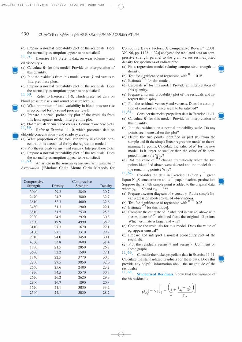
430 CHAPTER 11 SIMPLE LINEAR REGRESSION AND CORRELATION
(c) Prepare a normal probability plot of the residuals. Doesthe normality assumption appear to be satisfied?
11-57. Exercise 11-9 presents data on wear volume y andoil viscosity x.(a) Calculate R2 for this model. Provide an interpretation of
this quantity.(b) Plot the residuals from this model versus and versus x.
Interpret these plots.(c) Prepare a normal probability plot of the residuals. Does
the normality assumption appear to be satisfied?11-58. Refer to Exercise 11-8, which presented data onblood pressure rise y and sound pressure level x.(a) What proportion of total variability in blood pressure rise
is accounted for by sound pressure level?(b) Prepare a normal probability plot of the residuals from
this least squares model. Interpret this plot.(c) Plot residuals versus and versus x. Comment on these plots.11-59. Refer to Exercise 11-10, which presented data onchloride concentration y and roadway area x.(a) What proportion of the total variability in chloride con-
centration is accounted for by the regression model?(b) Plot the residuals versus and versus x. Interpret these plots.(c) Prepare a normal probability plot of the residuals. Does
the normality assumption appear to be satisfied?11-60. An article in the Journal of the American StatisticalAssociation [“Markov Chain Monte Carlo Methods for
y
y
y
Computing Bayes Factors: A Comparative Review” (2001,Vol. 96, pp. 1122–1132)] analyzed the tabulated data on com-pressive strength parallel to the grain versus resin-adjusteddensity for specimens of radiata pine.(a) Fit a regression model relating compressive strength to
density.(b) Test for significance of regression with .(c) Estimate for this model.(d) Calculate R2 for this model. Provide an interpretation of
this quantity.(e) Prepare a normal probability plot of the residuals and in-
terpret this display.(f ) Plot the residuals versus and versus x. Does the assump-
tion of constant variance seem to be satisfied?11-61. Consider the rocket propellant data in Exercise 11-11.(a) Calculate R2 for this model. Provide an interpretation of
this quantity.(b) Plot the residuals on a normal probability scale. Do any
points seem unusual on this plot?(c) Delete the two points identified in part (b) from the
sample and fit the simple linear regression model to the re-maining 18 points. Calculate the value of R2 for the newmodel. Is it larger or smaller than the value of R2 com-puted in part (a)? Why?
(d) Did the value of change dramatically when the twopoints identified above were deleted and the model fit tothe remaining points? Why?
11-62. Consider the data in Exercise 11-7 on y ϭ greenliquor Na2S concentration and x ϭ paper machine production.Suppose that a 14th sample point is added to the original data,where y14 ϭ 59 and x14 ϭ 855.(a) Prepare a scatter diagram of y versus x. Fit the simple lin-
ear regression model to all 14 observations.(b) Test for significance of regression with ␣ ϭ 0.05.(c) Estimate 2 for this model.(d) Compare the estimate of 2 obtained in part (c) above with
the estimate of 2 obtained from the original 13 points.Which estimate is larger and why?
(e) Compute the residuals for this model. Does the value ofe14 appear unusual?
(f ) Prepare and interpret a normal probability plot of theresiduals.
(g) Plot the residuals versus and versus x. Comment onthese graphs.
11-63. Consider the rocket propellant data in Exercise 11-11.Calculate the standardized residuals for these data. Does thisprovide any helpful information about the magnitude of theresiduals?11-64. Studentized Residuals. Show that the variance ofthe ith residual is
V1ei2 ϭ 2 c1 Ϫ a1n ϩ
1xi Ϫ x22Sxx
b d
y
2
y
2␣ ϭ 0.05
Compressive CompressiveStrength Density Strength Density
3040 29.2 3840 30.72470 24.7 3800 32.73610 32.3 4600 32.63480 31.3 1900 22.13810 31.5 2530 25.32330 24.5 2920 30.81800 19.9 4990 38.93110 27.3 1670 22.13160 27.1 3310 29.22310 24.0 3450 30.14360 33.8 3600 31.41880 21.5 2850 26.73670 32.2 1590 22.11740 22.5 3770 30.32250 27.5 3850 32.02650 25.6 2480 23.24970 34.5 3570 30.32620 26.2 2620 29.92900 26.7 1890 20.81670 21.1 3030 33.22540 24.1 3030 28.2
JWCL232_c11_401-448.qxd 1/14/10 8:03 PM Page 430

11-8 CORRELATION 431
11-8 CORRELATION
Our development of regression analysis has assumed that x is a mathematical variable, mea-sured with negligible error, and that Y is a random variable. Many applications of regressionanalysis involve situations in which both X and Y are random variables. In these situations, itis usually assumed that the observations (Xi, Yi), i ϭ 1, 2, p , n are jointly distributed randomvariables obtained from the distribution f (x, y).
For example, suppose we wish to develop a regression model relating the shear strengthof spot welds to the weld diameter. In this example, weld diameter cannot be controlled. Wewould randomly select n spot welds and observe a diameter (Xi) and a shear strength (Yi) foreach. Therefore (Xi, Yi) are jointly distributed random variables.
We assume that the joint distribution of Xi and Yi is the bivariate normal distribution pre-sented in Chapter 5, and Y and 2
Y are the mean and variance of Y, X and are the meanand variance of X, and is the correlation coefficient between Y and X. Recall that the corre-lation coefficient is defined as
(11-35)
where XY is the covariance between Y and X.The conditional distribution of Y for a given value of X ϭ x is
(11-36)
where
(11-37)
(11-38)
and the variance of the conditional distribution of Y given X ϭ x is
(11-39)2Y 0 x ϭ 2
Y 11 Ϫ 221 ϭ
YX
0 ϭ Y Ϫ XYX
fY 0 x 1 y2 ϭ1
12Y 0 x exp cϪ12ay Ϫ 0 Ϫ 1x
Y 0 x b2d
ϭXY
X Y
2X
Hint:
The ith studentized residual is defined as
(a) Explain why ri has unit standard deviation.(b) Do the standardized residuals have unit standard deviation?(c) Discuss the behavior of the studentized residual when the
sample value xi is very close to the middle of the range of x.
ri ϭei
B2 c1 Ϫ a1n ϩ
1xi Ϫ x 22Sxx
b d
cov1Yi, Yi2 ϭ 2 c 1n ϩ1xi Ϫ x 22
Sxxd .
(d) Discuss the behavior of the studentized residual when thesample value xi is very near one end of the range of x.
11-65. Show that an equivalent way to define the test forsignificance of regression in simple linear regression is to basethe test on R2 as follows: to test H0: 1 ϭ 0 versus H1: 1 ϶ 0,calculate
and to reject H0: 1 ϭ 0 if the computed value f0 Ͼ f␣,1,nϪ2.Suppose that a simple linear regression model has been fit ton ϭ 25 observations and R2 ϭ 0.90.(a) Test for significance of regression at ␣ ϭ 0.05.(b) What is the smallest value of R2 that would lead to the
conclusion of a significant regression if ␣ ϭ 0.05?
F0 ϭR21n Ϫ 22
1 Ϫ R2
JWCL232_c11_401-448.qxd 1/14/10 8:03 PM Page 431

432 CHAPTER 11 SIMPLE LINEAR REGRESSION AND CORRELATION
That is, the conditional distribution of Y given X ϭ x is normal with mean
(11-40)
and variance Thus, the mean of the conditional distribution of Y given X ϭ x is asimple linear regression model. Furthermore, there is a relationship between the correlationcoefficient and the slope 1. From Equation 11-38 we see that if ϭ 0, then 1 ϭ 0, whichimplies that there is no regression of Y on X. That is, knowledge of X does not assist us inpredicting Y.
The method of maximum likelihood may be used to estimate the parameters 0 and 1. Itcan be shown that the maximum likelihood estimators of those parameters are
(11-41)
and
(11-42)
We note that the estimators of the intercept and slope in Equations 11-41 and 11-42 areidentical to those given by the method of least squares in the case where X was assumed to bea mathematical variable. That is, the regression model with Y and X jointly normally distrib-uted is equivalent to the model with X considered as a mathematical variable. This followsbecause the random variables Y given X ϭ x are independently and normally distributed withmean 0 ϩ 1x and constant variance These results will also hold for any joint distribu-tion of Y and X such that the conditional distribution of Y given X is normal.
It is possible to draw inferences about the correlation coefficient in this model. Theestimator of is the sample correlation coefficient
(11-43)
Note that
(11-44)
so the slope is just the sample correlation coefficient R multiplied by a scale factor that isthe square root of the “spread” of the Y values divided by the “spread” of the X values.Thus,
and R are closely related, although they provide somewhat different information. Thesample correlation coefficient R measures the linear association between Y and X, while measures the predicted change in the mean of Y for a unit change in X. In the case of a math-ematical variable x, R has no meaning because the magnitude of R depends on the choice ofspacing of x. We may also write, from Equation 11-44,
R2 ϭ 21
SX X
SSTϭ
1SX Y
SSTϭ
SSR
SST
1
1
1
1 ϭ aSST
SX Xb1ր 2
R
R ϭa
n
iϭ1Yi 1Xi Ϫ X 2
c aniϭ11Xi Ϫ X 22 an
iϭ11Yi Ϫ Y 22 d 1ր2 ϭ
SX Y1SX XSST21ր2
2Y 0 x.
1 ϭa
n
iϭ1Yi 1Xi Ϫ X 2
an
iϭ11Xi Ϫ X 22 ϭ
SXY
SX X
0 ϭ Y Ϫ 1X
2Y 0 x.
E1Y 0 x2 ϭ 0 ϩ 1x
JWCL232_c11_401-448.qxd 1/14/10 8:04 PM Page 432

11-8 CORRELATION 433
which is just the coefficient of determination. That is, the coefficient of determination R2 isjust the square of the correlation coefficient between Y and X.
It is often useful to test the hypotheses
(11-45)
The appropriate test statistic for these hypotheses is
H1: � 0H0: ϭ 0
ConfidenceInterval for
a CorrelationCoefficient
(11-49)Z0 ϭ 1arctanh R Ϫ arctanh 02 1n Ϫ 321ր2
(11-50)tanh aarctanh r Ϫz␣ր2
1n Ϫ 3b Յ Յ tanh aarctanh r ϩ
z␣ր2
1n Ϫ 3b
which has the t distribution with n Ϫ 2 degrees of freedom if H0: ϭ 0 is true. Therefore, wewould reject the null hypothesis if t0 Ͼ t␣2,nϪ2. This test is equivalent to the test of the hypothesisH0: 1 ϭ 0 given in Section 11-5.1. This equivalence follows directly from Equation 11-46.
The test procedure for the hypotheses
(11-47)
where 0 ϶ 0 is somewhat more complicated. For moderately large samples (say, n Ն 25), thestatistic
(11-48)
is approximately normally distributed with mean and variance
respectively. Therefore, to test the hypothesis H0: ϭ 0, we may use the test statistic
Z ϭ arctanh ϭ12
ln 1 ϩ
1 Ϫ and 2
Z ϭ1
n Ϫ 3
Z ϭ arctanh R ϭ12
ln1 ϩ R1 Ϫ R
H1: � 0
H0: ϭ 0
and reject H0: ϭ 0 if the value of the test statistic in Equation 11-49 is such that z0 Ͼ z␣2.It is also possible to construct an approximate 100(1 Ϫ ␣)% confidence interval for , using
the transformation in Equation 11-48. The approximate 100(1 Ϫ ␣)% confidence interval is
(11-46)T0 ϭR1n Ϫ 2
21 Ϫ R2
Test Statisticfor Zero
Correlation
where tanh u ϭ (eu Ϫ eϪu )(eu ϩ eϪu ).
JWCL232_c11_401-448.qxd 1/14/10 8:04 PM Page 433

434 CHAPTER 11 SIMPLE LINEAR REGRESSION AND CORRELATION
Figure 11-13 Scatterplot of wire bondstrength versus wirelength, Example 11-8.
0
10
20
30
40
50
60
70
0 5 10 15 20
Str
ength
Wire length
Regression Analysis: Strength versus Length
The regression equation isStrength ϭ 5.11 ϩ 2.90 Length
Predictor Coef SE Coef T PConstant 5.115 1.146 4.46 0.000Length 2.9027 0.1170 24.80 0.000
S ϭ 3.093 R-Sq ϭ 96.4% R-Sq(adj) ϭ 96.2%PRESS ϭ 272.144 R-Sq(pred) ϭ 95.54%
Analysis of Variance
Source DF SS MS F PRegression 1 5885.9 5885.9 615.08 0.000Residual Error 23 220.1 9.6Total 24 6105.9
EXAMPLE 11-8 Wire Bond Pull StrengthIn Chapter 1 (Section 1-3) an application of regression analysisis described in which an engineer at a semiconductor assemblyplant is investigating the relationship between pull strength of awire bond and two factors: wire length and die height. In this ex-ample, we will consider only one of the factors, the wire length.A random sample of 25 units is selected and tested, and the wirebond pull strength and wire length are observed for each unit.The data are shown in Table 1-2. We assume that pull strengthand wire length are jointly normally distributed.
Figure 11-13 shows a scatter diagram of wire bondstrength versus wire length. We have used the Minitab optionof displaying box plots of each individual variable on the scat-ter diagram. There is evidence of a linear relationship betweenthe two variables.
The Minitab output for fitting a simple linear regressionmodel to the data is shown below.
Now Sxx ϭ 698.56 and Sxy ϭ 2027.7132, and the samplecorrelation coefficient is
Note that r2 ϭ (0.9818)2 ϭ 0.9640 (which is reported in theMinitab output), or that approximately 96.40% of the variabilityin pull strength is explained by the linear relationship to wirelength.
Now suppose that we wish to test the hypotheses
H1: � 0
H0: ϭ 0
r ϭSxy3Sx xSST 41ր2 ϭ
2027.71323 1698.5602 16105.92 41ր2 ϭ 0.9818
JWCL232_c11_401-448.qxd 1/14/10 8:04 PM Page 434
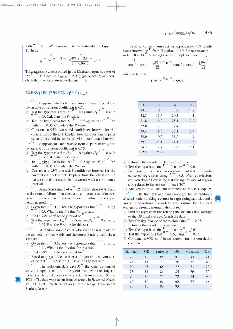
EXERCISES FOR SECTION 11–8
11-8 CORRELATION 435
with ␣ ϭ 0.05. We can compute the t-statistic of Equation11-46 as
This statistic is also reported in the Minitab output as a test ofH0: 1 ϭ 0. Because t0.025,23 ϭ 2.069, we reject H0 and con-clude that the correlation coefficient � 0.
t0 ϭr1n Ϫ 2
21 Ϫ r2ϭ
0.981812311 Ϫ 0.9640
ϭ 24.8
Finally, we may construct an approximate 95% confi-dence interval on from Equation 11-50. Since arctanh r ϭ
arctanh 0.9818 ϭ 2.3452, Equation 11-50 becomes
which reduces to
0.9585 Յ Յ 0.9921
tanh a2.3452 Ϫ1.96122b Յ Յ tanh a2.3452 ϩ
1.96122b
11-66. Suppose data is obtained from 20 pairs of (x, y) andthe sample correlation coefficient is 0.8.(a) Test the hypothesis that against with
. Calculate the P-value.(b) Test the hypothesis that against
with . Calculate the P-value.(c) Construct a 95% two-sided confidence interval for the
correlation coefficient. Explain how the questions in parts(a) and (b) could be answered with a confidence interval.
11-67. Suppose data are obtained from 20 pairs of (x, y) andthe sample correlation coefficient is 0.75.(a) Test the hypothesis that against with
. Calculate the P-value.(b) Test the hypothesis that against
with . Calculate the P-value.(c) Construct a 95% one-sided confidence interval for the
correlation coefficient. Explain how the questions inparts (a) and (b) could be answered with a confidenceinterval.
11-68. A random sample of n ϭ 25 observations was madeon the time to failure of an electronic component and the tem-perature in the application environment in which the compo-nent was used.(a) Given that r ϭ 0.83, test the hypothesis that ϭ 0, using
␣ ϭ 0.05. What is the P-value for this test?(b) Find a 95% confidence interval on .(c) Test the hypothesis H0: ϭ 0.8 versus H1: ϶ 0.8, using
␣ ϭ 0.05. Find the P-value for this test.11-69. A random sample of 50 observations was made onthe diameter of spot welds and the corresponding weld shearstrength.(a) Given that r ϭ 0.62, test the hypothesis that ϭ 0, using
␣ ϭ 0.01. What is the P-value for this test?(b) Find a 99% confidence interval for .(c) Based on the confidence interval in part (b), can you con-
clude that ϭ 0.5 at the 0.01 level of significance?11-70. The following data gave X ϭ the water content ofsnow on April 1 and Y ϭ the yield from April to July (ininches) on the Snake River watershed in Wyoming for 1919 to1935. (The data were taken from an article in Research Notes,Vol. 61, 1950, Pacific Northwest Forest Range ExperimentStation, Oregon.)
␣ ϭ 0.05H1: Ͼ 0.5H1: ϭ 0.5
␣ ϭ 0.05H1: Ͼ 0H0: ϭ 0
␣ ϭ 0.05H1: � 0.5H1: ϭ 0.5
␣ ϭ 0.05H1: � 0H0: ϭ 0
x y x y
23.1 10.5 37.9 22.832.8 16.7 30.5 14.131.8 18.2 25.1 12.932.0 17.0 12.4 8.830.4 16.3 35.1 17.424.0 10.5 31.5 14.939.5 23.1 21.1 10.524.2 12.4 27.6 16.152.5 24.9
(a) Estimate the correlation between Y and X.(b) Test the hypothesis that ϭ 0, using ␣ ϭ 0.05.(c) Fit a simple linear regression model and test for signifi-
cance of regression using ␣ ϭ 0.05. What conclusionscan you draw? How is the test for significance of regres-sion related to the test on in part (b)?
(d) Analyze the residuals and comment on model adequacy.11-71. The final test and exam averages for 20 randomlyselected students taking a course in engineering statistics and acourse in operations research follow. Assume that the finalaverages are jointly normally distributed.(a) Find the regression line relating the statistics final average
to the OR final average. Graph the data.(b) Test for significance of regression using ␣ ϭ 0.05.(c) Estimate the correlation coefficient.(d) Test the hypothesis that ϭ 0, using ␣ ϭ 0.05.(e) Test the hypothesis that ϭ 0.5, using ␣ ϭ 0.05.(f) Construct a 95% confidence interval for the correlation
coefficient.
Statistics OR Statistics OR Statistics OR
86 80 86 81 83 8175 81 71 76 75 7069 75 65 72 71 7375 81 84 85 76 7290 92 71 72 84 8094 95 62 65 97 9883 80 90 93
JWCL232_c11_401-448.qxd 1/14/10 8:04 PM Page 435

11-72. The weight and systolic blood pressure of 26 ran-domly selected males in the age group 25 to 30 are shown inthe following table. Assume that weight and blood pressureare jointly normally distributed.
436 CHAPTER 11 SIMPLE LINEAR REGRESSION AND CORRELATION
(a) Graph the data and fit a regression line to predict cur-rent without electronics to supply voltage. Is there a significant regression at ? What is the P-value?
(b) Estimate the correlation coefficient.(c) Test the hypothesis that against the alternative
with . What is the P-value?(d) Compute a 95% confidence interval for the correlation
coefficient.11-74. The monthly absolute estimate of global (landand ocean combined) temperature indexes (degrees C) in2000 and 2001 are (source: http://www.ncdc.noaa.gov/oa/climate/):
2000: 12.28, 12.63, 13.22, 14.21, 15.13, 15.82, 16.05,16.02, 15.29, 14.29, 13.16, 12.47
2001: 12.44, 12.55, 13.35, 14.22, 15.28, 15.99, 16.23,16.17, 15.44, 14.52, 13.52, 12.61
(a) Graph the data and fit a regression line to predict 2001temperatures from those in 2000. Is there a significantregression at ? What is the P-value?
(b) Estimate the correlation coefficient.(c) Test the hypothesis that against the alternative
with . What is the P-value?(d) Compute a 95% confidence interval for the correlation
coefficient.11-75 Refer to the NFL quarterback ratings data inExercise 11-3.(a) Estimate the correlation coefficient between the rat-
ings and the average yards per attempt.(b) Test the hypothesis versus using
. What is the P-value for this test?(c) Construct a 95% confidence interval for .(d) Test the hypothesis versus us-
ing . Find the P-value for this test.11-76. Consider the following (x, y) data. Calculatethe correlation coefficient. Graph the data and commenton the relationship between x and y. Explain why thecorrelation coefficient does not detect the relationshipbetween x and y.
␣ ϭ 0.05H1: � 0.7H0: ϭ 0.7
␣ ϭ 0.05H1: � 0H0: ϭ 0
␣ ϭ 0.05 � 0.9 ϭ 0.9
␣ ϭ 0.05
␣ ϭ 0.05 � 0 ϭ 0
␣ ϭ 0.05
SystolicSubject Weight BP
1 165 1302 167 1333 180 1504 155 1285 212 1516 175 1467 190 1508 210 1409 200 148
10 149 12511 158 13312 169 13513 170 150
SystolicSubject Weight BP
14 172 15315 159 12816 168 13217 174 14918 183 15819 215 15020 195 16321 180 15622 143 12423 240 17024 235 16525 192 16026 187 159
(a) Find a regression line relating systolic blood pressure toweight.
(b) Test for significance of regression using ␣ ϭ 0.05.(c) Estimate the correlation coefficient.(d) Test the hypothesis that ϭ 0, using ␣ ϭ 0.05.(e) Test the hypothesis that ϭ 0.6, using ␣ ϭ 0.05.(f) Construct a 95% confidence interval for the correlation
coefficient.11-73. In an article in IEEE Transactions on Instrumentationand Measurement (2001, Vol. 50, pp. 986–990), researchersstudied the effects of reducing current draw in a magnetic coreby electronic means. They measured the current in a magneticwinding with and without the electronics in a paired experi-ment. Data for the case without electronics are provided in thefollowing table.
Current WithoutSupply Voltage Electronics (mA)
0.66 7.321.32 12.221.98 16.342.64 23.663.3 28.063.96 33.394.62 34.123.28 39.215.94 44.216.6 47.48
x y
0
2.65
3.46
3.870 4
Ϫ1Ϫ3.87Ϫ1
Ϫ2Ϫ3.46Ϫ2
Ϫ3Ϫ2.65Ϫ3
Ϫ4
x y
01 3.8712 3.4623 2.6534 0
Ϫ2.65
Ϫ3.46
Ϫ3.87
Ϫ4
JWCL232_c11_401-448.qxd 1/14/10 8:04 PM Page 436
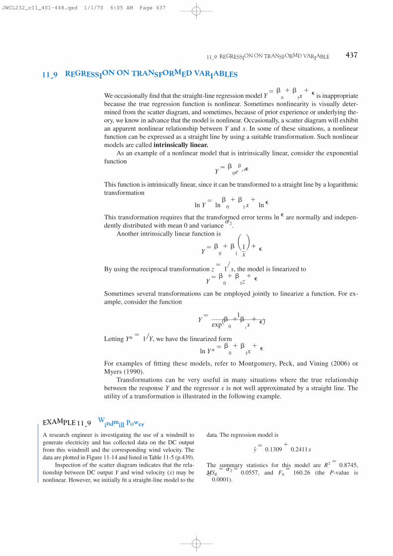
11-9 REGRESSION ON TRANSFORMD VARIABLE 437
11-9 REGRESSION ON TRANSFORMED VARIABLES
We occasionally find that the straight-line regression model Y ϭ 0 ϩ 1x ϩ ⑀ is inappropriatebecause the true regression function is nonlinear. Sometimes nonlinearity is visually deter-mined from the scatter diagram, and sometimes, because of prior experience or underlying the-ory, we know in advance that the model is nonlinear. Occasionally, a scatter diagram will exhibitan apparent nonlinear relationship between Y and x. In some of these situations, a nonlinearfunction can be expressed as a straight line by using a suitable transformation. Such nonlinearmodels are called intrinsically linear.
As an example of a nonlinear model that is intrinsically linear, consider the exponentialfunction
This function is intrinsically linear, since it can be transformed to a straight line by a logarithmictransformation
This transformation requires that the transformed error terms ln ⑀ are normally and indepen-dently distributed with mean 0 and variance 2.
Another intrinsically linear function is
By using the reciprocal transformation z ϭ 1x, the model is linearized to
Sometimes several transformations can be employed jointly to linearize a function. For ex-ample, consider the function
Letting , we have the linearized form
For examples of fitting these models, refer to Montgomery, Peck, and Vining (2006) orMyers (1990).
Transformations can be very useful in many situations where the true relationshipbetween the response Y and the regressor x is not well approximated by a straight line. Theutility of a transformation is illustrated in the following example.
ln Y* ϭ 0 ϩ 1x ϩ ⑀
Y* ϭ 1րY
Y ϭ1
exp 10 ϩ 1x ϩ ⑀2
Y ϭ 0 ϩ 1z ϩ ⑀
Y ϭ 0 ϩ 1a1xb ϩ ⑀
ln Y ϭ ln 0 ϩ 1x ϩ ln ⑀
Y ϭ 0e1x⑀
EXAMPLE 11-9 Windmill PowerA research engineer is investigating the use of a windmill togenerate electricity and has collected data on the DC outputfrom this windmill and the corresponding wind velocity. Thedata are plotted in Figure 11-14 and listed in Table 11-5 (p.439).
Inspection of the scatter diagram indicates that the rela-tionship between DC output Y and wind velocity (x) may benonlinear. However, we initially fit a straight-line model to the
data. The regression model is
The summary statistics for this model are R2 ϭ 0.8745,, and F0 ϭ 160.26 (the P-value isMSE ϭ 2 ϭ 0.0557
y ϭ 0.1309 ϩ 0.2411x
Ͻ0.0001).
JWCL232_c11_401-448.qxd 1/1/70 6:05 AM Page 437

438 CHAPTER 11 SIMPLE LINEAR REGRESSION AND CORRELATION
A plot of the residuals versus is shown in Figure 11-15.This residual plot indicates model inadequacy and implies thatthe linear relationship has not captured all of the informationin the wind speed variable. Note that the curvature that was ap-parent in the scatter diagram of Figure 11-14 is greatlyamplified in the residual plots. Clearly some other model formmust be considered.
We might initially consider using a quadratic model such as
to account for the apparent curvature. However, the scatter di-agram of Figure 11-14 suggests that as wind speed increases,DC output approaches an upper limit of approximately 2.5.This is also consistent with the theory of windmill operation.Since the quadratic model will eventually bend downward aswind speed increases, it would not be appropriate for thesedata. A more reasonable model for the windmill data that in-corporates an upper asymptote would be
y ϭ 0 ϩ 1 a1xb ϩ ⑀
y ϭ 0 ϩ 1x ϩ 2 x2 ϩ ⑀
yi
1.0
20
2.0
3.0
0.0
DC
outp
ut,
y
4 6 8 10
Wind velocity, x
Figure 11-14 Plot of DC output y versus wind velocity xfor the windmill data.
0.4
0.2
0.0
–0.2
–0.4
–0.6
0.4
ei
0.8 1.2 1.6 2.0 2.4
y
Figure 11-15 Plot of residuals ei versus fittedvalues for the windmill data.yi
1.0
3.0
0.00.10
2.0
DC
outp
ut,
y
0.20 0.30 0.40 0.50
x' =1x
Figure 11-16 Plot of DC output versus for thewindmill data.
x¿ ϭ 1րx
ei
–0.4
–0.610
–0.2
0
0.2
0.4
2 3
yi
Figure 11-17 Plot of residuals versus fitted values for the transformed modelfor the windmill data.
yi
Figure 11-16 is a scatter diagram with the transformed variable. This plot appears linear, indicating that the reciprocal
transformation is appropriate. The fitted regression model is
The summary statistics for this model are R2 ϭ 0.9800,, and F0 ϭ 1128.43 (the P value is
Ͻ0.0001).A plot of the residuals from the transformed model ver-
sus is shown in Figure 11-17. This plot does not reveal anyserious problem with inequality of variance. The normal prob-ability plot, shown in Figure 11-18, gives a mild indicationthat the errors come from a distribution with heavier tails thanthe normal (notice the slight upward and downward curve atthe extremes). This normal probability plot has the z-scorevalue plotted on the horizontal axis. Since there is no strongsignal of model inadequacy, we conclude that the transformedmodel is satisfactory.
y
MSE ϭ 2 ϭ 0.0089
y ϭ 2.9789 Ϫ 6.9345x¿
x¿ ϭ 1րx
JWCL232_c11_401-448.qxd 1/18/10 2:17 PM Page 438

11-9 REGRESSION ON TRANSFORMED VARIABLES 439
ei
–0.4
–0.6–1–2
–0.2
0
0.2
0.4
0 21
zi
Figure 11-18 Normal probability plot ofthe residuals for the transformed model forthe windmill data.
EXERCISES FOR SECTION 11–9
11-77. Determine if the following models are intrinsicallylinear. If yes, determine the appropriate transformation togenerate the linear model.
(a) (b)
(c) (d)
11-78. The vapor pressure of water at various temperaturesfollows:
Y ϭx
0x ϩ 1 ϩ x⑀Y ϭ 0
x1⑀
Y ϭ3 ϩ 5x
x ϩ ⑀Y ϭ 0x1⑀
(a) Draw a scatter diagram of these data. What type ofrelationship seems appropriate in relating y to x?
Observation Vapor pressureNumber, i Temperature (K) (mm Hg)
1 273 4.62 283 9.23 293 17.54 303 31.85 313 55.36 323 92.57 333 149.48 343 233.79 353 355.1
10 363 525.811 373 760.0
(b) Fit a simple linear regression model to these data.(c) Test for significance of regression using ␣ ϭ 0.05. What
conclusions can you draw?(d) Plot the residuals from the simple linear regression model
versus . What do you conclude about model adequacy?yi
Customer x y Customer x y
1 679 0.79 26 1434 0.312 292 0.44 27 837 4.203 1012 0.56 28 1748 4.884 493 0.79 29 1381 3.485 582 2.70 30 1428 7.586 1156 3.64 31 1255 2.637 997 4.73 32 1777 4.998 2189 9.50 33 370 0.599 1097 5.34 34 2316 8.19
10 2078 6.85 35 1130 4.79continued
(e) The Clausis–Clapeyron relationship states that lnwhere is the vapor pressure of water. Repeat parts (a)–(d). using an appropriate transformation.
11-79. An electric utility is interested in developing a modelrelating peak hour demand ( y in kilowatts) to total monthlyenergy usage during the month (x, in kilowatt hours). Data for50 residential customers are shown in the following table.
Pv
1Pv2�Ϫ 1T ,
Table 11-5 Observed Values yi and Regressor Variable xi
for Example 11-9
Observation Wind Velocity DC Output,Number, i (mph), xi yi
1 5.00 1.5822 6.00 1.8223 3.40 1.057
Observation Wind Velocity DC Output,Number, i (mph), xi yi
4 2.70 0.5005 10.00 2.2366 9.70 2.3867 9.55 2.2948 3.05 0.5589 8.15 2.166
10 6.20 1.86611 2.90 0.65312 6.35 1.93013 4.60 1.56214 5.80 1.73715 7.40 2.08816 3.60 1.13717 7.85 2.17918 8.80 2.11219 7.00 1.80020 5.45 1.50121 9.10 2.30322 10.20 2.31023 4.10 1.19424 3.95 1.14425 2.45 0.123continued
JWCL232_c11_401-448.qxd 1/1/70 6:04 AM Page 439

440 CHAPTER 11 SIMPLE LINEAR REGRESSION AND CORRELATION
Customer x y Customer x y
11 1818 5.84 36 463 0.5112 1700 5.21 37 770 1.7413 747 3.25 38 724 4.1014 2030 4.43 39 808 3.9415 1643 3.16 40 790 0.9616 414 0.50 41 783 3.2917 354 0.17 42 406 0.4418 1276 1.88 43 1242 3.2419 745 0.77 44 658 2.1420 795 3.70 45 1746 5.7121 540 0.56 46 895 4.1222 874 1.56 47 1114 1.9023 1543 5.28 48 413 0.5124 1029 0.64 49 1787 8.3325 710 4.00 50 3560 14.94
(a) Draw a scatter diagram of y versus x.(b) Fit the simple linear regression model.(c) Test for significance of regression using ␣ ϭ 0.05.(d) Plot the residuals versus and comment on the underly-
ing regression assumptions. Specifically, does it seem thatthe equality of variance assumption is satisfied?
(e) Find a simple linear regression model using as theresponse. Does this transformation on y stabilize the in-equality of variance problem noted in part (d) above?
1y
yi
11-10 LOGISTIC REGRESSION
Linear regression often works very well when the response variable is quantitative. We nowconsider the situation where the response variable takes on only two possible values, 0 and1. These could be arbitrary assignments resulting from observing a qualitative response.For example, the response could be the outcome of a functional electrical test on a semi-conductor device for which the results are either a “success,” which means the device worksproperly, or a “failure,” which could be due to a short, an open, or some other functionalproblem.
Suppose that the model has the form
(11-51)
and the response variable Yi takes on the values either 0 or 1. We will assume that the responsevariable Yi is a Bernoulli random variable with probability distribution as follows:
Yi ϭ 0 ϩ 1xi ϩ ⑀i
Yi Probability
10 P1Yi ϭ 02 ϭ 1 Ϫ i
P1Yi ϭ 12 ϭ i
Now since the expected value of the response variable is
This implies that
E 1Yi2 ϭ 0 ϩ 1xi ϭ i
ϭ i
E 1Yi2 ϭ 1 1i2 ϩ 0 11 Ϫ i2E 1⑀i2 ϭ 0,
JWCL232_c11_401-448.qxd 1/14/10 8:04 PM Page 440

11-10 LOGISTIC REGRESSION 441
This means that the expected response given by the response function E(Yi) ϭ 0 ϩ 1xi isjust the probability that the response variable takes on the value 1.
There are some substantive problems with the regression model in Equation 11-51. First,note that if the response is binary, the error terms ⑀i can only take on two values, namely,
Consequently, the errors in this model cannot possibly be normal. Second, the error varianceis not constant, since
Notice that this last expression is just
since . This indicates that the variance of the observations (which isE1Yi2 ϭ 0 ϩ 1xi ϭ i
2yi
ϭ E1Yi2 31 Ϫ E1Yi2 4ϭ i11 Ϫ i2ϭ 11 Ϫ i22i ϩ 10 Ϫ i2211 Ϫ i22
Yiϭ E5Yi Ϫ E1Yi2 62
⑀i ϭ Ϫ10 ϩ 1 xi2 when Yi ϭ 0
⑀i ϭ 1 Ϫ 10 ϩ 1 xi2 when Yi ϭ 1
0
0.2
0.4
0.6
0.8
1
1.2
0 2 4 6 8 10 12 14
E(Y )
x
(a)
0
0.2
0.4
0.6
0.8
1
1.2
0 2 4 6 8 10 12 14
E(Y )
x
(b)
Figure 11-19 Examples of the logistic response function. (a) (b) .E1Y 2 ϭ 1ր 11 ϩ eϪ6.0ϩ1.0x2E1Y 2 ϭ 1ր 11 ϩ eϪ6.0Ϫ1.0x2,
the same as the variance of the errors because ϭ Yi Ϫ i, and i is a constant) is a functionof the mean. Finally, there is a constraint on the response function, because
This restriction can cause serious problems with the choice of a linear response function, aswe have initially assumed in Equation 11-51. It would be possible to fit a model to the data forwhich the predicted values of the response lie outside the 0, 1 interval.
Generally, when the response variable is binary, there is considerable empirical evidenceindicating that the shape of the response function should be nonlinear. A monotonicallyincreasing (or decreasing) S-shaped (or reverse S-shaped) function, such as shown in Figure 11-19,is usually employed. This function is called the logit response function, and has the form
(11-52)E1Y 2 ϭexp 10 ϩ 1x2
1 ϩ exp 10 ϩ 1x2
0 Յ E 1Yi2 ϭ i Յ 1
⑀i
JWCL232_c11_401-448.qxd 1/14/10 8:05 PM Page 441

or equivalently,
(11-53)
In logistic regression we assume that E(Y ) is related to x by the logit function. It is easy toshow that
(11-54)
The quantity exp( ) on the right-hand side of Equation 11-54 is called the odds ratio.It has a straightforward interpretation: If the odds ratio is 2 for a particular value of x, it meansthat a success is twice as likely as a failure at that value of the regressor x. Notice that thenatural logarithm of the odds ratio is a linear function of the regressor variable. Therefore theslope is the change in the log odds that results from a one-unit increase in x. This means thatthe odds ratio changes by when x increases by one unit.
The parameters in this logistic regression model are usually estimated by the method ofmaximum likelihood. For details of the procedure, see Montgomery, Peck, and Vining(2006). Minitab will fit logistic regression models and provide useful information on thequality of the fit.
We will illustrate logistic regression using the data on launch temperature and O-ring fail-ure for the 24 space shuttle launches prior to the Challenger disaster of January 1986. Thereare six O-rings used to seal field joints on the rocket motor assembly. The table below presentsthe launch temperatures. A 1 in the “O-Ring Failure” column indicates that at least one O-ringfailure had occurred on that launch.
e1
1
0 ϩ 1x
E1Y 21 Ϫ E1Y 2 ϭ exp10 ϩ 1x2
E1Y 2 ϭ1
1 ϩ exp 3Ϫ10 ϩ 1x2 4
442 CHAPTER 11 SIMPLE LINEAR REGRESSION AND CORRELATION
O-Ring O-Ring O-Ring Temperature Failure Temperature Failure Temperature Failure
53 1 68 0 75 056 1 69 0 75 157 1 70 0 76 063 0 70 1 76 066 0 70 1 78 067 0 70 1 79 067 0 72 0 80 067 0 73 0 81 0
Figure 11-20 is a scatter plot of the data. Note that failures tend to occur at lower temperatures.The logistic regression model fit to this data from Minitab is shown in the following boxeddisplay.
The fitted logistic regression model is
y ϭ1
1 ϩ exp 3Ϫ110.875 Ϫ 0.17132x2 4
JWCL232_c11_401-448.qxd 1/15/10 4:54 PM Page 442

11-10 LOGISTIC REGRESSION 443
Binary Logistic Regression: O-Ring Failure versus Temperature
Link Function: LogitResponse Information
Variable Value CountO-Ring F 1 7 (Event)
0 17Total 24
Logistic Regression Table
Odds 95% CIPredictor Coef SE Coef Z P Ratio Lower UpperConstant 10.875 5.703 1.91 0.057Temperat Ϫ0.17132 0.08344 Ϫ2.05 0.040 0.84 0.72 0.99
Log-Likelihood ϭ Ϫ11.515Test that all slopes are zero: G ϭ 5.944, DF ϭ 1, P-Value ϭ 0.015
Figure 11-20 Scatter plot of O-ring failures versus launch temperature for 24 space shuttleflights.
Figure 11-21 Probability of O-ring failure versuslaunch temperature (based on a logistic regressionmodel).
0.0
6050
0.5
1.0
O-r
ing f
ailure
70 80
Temperature
0.0
6050
0.5
1.0
P(O
-rin
g f
ailure
)
70 80
Temperature
The standard error of the slope 1 is se(1) ϭ 0.08344. For large samples, 1 has anapproximate normal distribution, and so 1se(1) can be compared to the standard normaldistribution to test H0: 1 ϭ 0. Minitab performs this test. The P-value is 0.04, indicating thattemperature has a significant effect on the probability of O-ring failure. The odds ratio is 0.84,so every one degree increase in temperature reduces the odds of failure by 0.84. Figure 11-21shows the fitted logistic regression model. The sharp increase in the probability of O-ringfailure is very evident in this graph. The actual temperature at the Challenger launch was .This is well outside the range of other launch temperatures, so our logistic regression model isnot likely to provide highly accurate predictions at that temperature, but it is clear that a launchat is almost certainly going to result in O-ring failure.
It is interesting to note that all of these data were available prior to launch. However,engineers were unable to effectively analyze the data and use them to provide a convincingargument against launching Challenger to NASA managers. Yet a simple regression analysis
31ЊF
31ЊF
JWCL232_c11_401-448.qxd 1/14/10 8:05 PM Page 443

444 CHAPTER 11 SIMPLE LINEAR REGRESSION AND CORRELATION
of the data would have provided a strong quantitative basis for this argument. This is one ofthe more dramatic instances that points out why engineers and scientists need a strongbackground in basic statistical techniques.
EXERCISES FOR SECTION 11–10
11-80 A study was conducted attempting to relate homeownership to family income. Twenty households were selectedand family income was estimated, along with information con-cerning home ownership (y ϭ 1 indicates yes and y ϭ 0indicates no). The data are shown below.
HomeOwnership
Household Income Status
1 38,000 02 51,200 13 39,600 04 43,400 15 47,700 06 53,000 07 41,500 18 40,800 09 45,400 1
10 52,400 111 38,700 112 40,100 013 49,500 114 38,000 015 42,000 116 54,000 117 51,700 118 39,400 019 40,900 020 52,800 1
Load, x (psi) Sample Size, n Number Failing, r
2500 50 102700 70 172900 100 303100 60 213300 40 183500 85 433700 90 543900 50 334100 80 604300 65 51
NumberDiscount, x Sample Size, n Redeemed, r
5 500 1007 500 1229 500 147
11 500 17613 500 21115 500 24417 500 27719 500 31021 500 34323 500 37225 500 391
(a) Fit a logistic regression model to the response variable y.Use a simple linear regression model as the structure forthe linear predictor.
(b) Is the logistic regression model in part (a) adequate?(c) Provide an interpretation of the parameter 1 in this model.11-81 The compressive strength of an alloy fastener usedin aircraft construction is being studied. Ten loads were se-lected over the range 2500– 4300 psi and a number of fasten-ers were tested at those loads. The numbers of fasteners failingat each load were recorded. The complete test data follow.
(a) Fit a logistic regression model to the data. Use a simplelinear regression model as the structure for the linear pre-dictor.
(b) Is the logistic regression model in part (a) adequate?11-82 The market research department of a soft drink man-ufacturer is investigating the effectiveness of a price discountcoupon on the purchase of a two-liter beverage product. Asample of 5500 customers was given coupons for varyingprice discounts between 5 and 25 cents. The response variablewas the number of coupons in each price discount category re-deemed after one month. The data are shown below.
(a) Fit a logistic regression model to the data. Use a simple lin-ear regression model as the structure for the linear predictor.
(b) Is the logistic regression model in part (a) adequate?(c) Draw a graph of the data and the fitted logistic regression
model.
JWCL232_c11_401-448.qxd 1/19/10 8:59 PM Page 444

11-10 LOGISTIC REGRESSION 445
(d) Expand the linear predictor to include a quadratic term. Isthere any evidence that this quadratic term is required inthe model?
(e) Draw a graph of this new model on the same plot that you pre-pared in part (c). Does the expanded model visually provide abetter fit to the data than the original model from part (a)?
11-83 A study was performed to investigate new automobilepurchases. A sample of 20 families was selected. Each family wassurveyed to determine the age of their oldest vehicle and their to-tal family income. A follow-up survey was conducted six monthslater to determine if they had actually purchased a new vehicleduring that time period ( y = 1 indicates yes and y = 0 indicatesno). The data from this study are shown in the following table.
Income, x1 Age, x2 y Income, x1 Age, x2 y
45,000 2 0 37,000 5 140,000 4 0 31,000 7 160,000 3 1 40,000 4 150,000 2 1 75,000 2 055,000 2 0 43,000 9 150,000 5 1 49,000 2 035,000 7 1 37,500 4 165,000 2 1 71,000 1 053,000 2 0 34,000 5 048,000 1 0 27,000 6 0
(a) Fit a logistic regression model to the data.(b) Is the logistic regression model in part (a) adequate?(c) Interpret the model coefficients 1 and 2.(d) What is the estimated probability that a family with an in-
come of $45,000 and a car that is five years old will pur-chase a new vehicle in the next six months?
(e) Expand the linear predictor to include an interaction term.Is there any evidence that this term is required in the model?
(a) Draw a scatter diagram of these data. Does a straight-linerelationship seem plausible?
(b) Fit a simple linear regression model to these data.(c) Test for significance of regression using ␣ ϭ 0.05. What
is the P-value for this test?(d) Find a 95% confidence interval estimate on the slope.(e) Test the hypothesis H0: 0 ϭ 0 versus H1: 0 ϶ 0 using
␣ ϭ 0.05. What conclusions can you draw?11-86. The strength of paper used in the manufacture of card-board boxes ( y) is related to the percentage of hardwood con-centration in the original pulp (x). Under controlled conditions, apilot plant manufactures 16 samples, each from a different batchof pulp, and measures the tensile strength. The data are shownin the table that follows:
y x y x
0.734 1.1 1.50 1.60.886 1.2 1.66 1.71.04 1.3 1.81 1.81.19 1.4 1.97 1.91.35 1.5 2.12 2.0
(a) Fit a simple linear regression model to the data.(b) Test for significance of regression using ␣ ϭ 0.05.(c) Construct a 90% confidence interval on the slope 1.(d) Construct a 90% confidence interval on the intercept 0.(e) Construct a 95% confidence interval on the mean strength
at x ϭ 2.5.(f) Analyze the residuals and comment on model adequacy.11-87. Consider the following data. Suppose that therelationship between Y and x is hypothesized to beY ϭ (0 ϩ 1x ϩ ⑀)Ϫ1. Fit an appropriate model to the data.Does the assumed model form seem reasonable?
x 10 15 18 12 9 8 11 6
y 0.1 0.13 0.09 0.15 0.20 0.21 0.18 0.24
y 101.4 117.4 117.1 106.2
x 1.0 1.5 1.5 1.5
y 131.9 146.9 146.8 133.9
x 2.0 2.0 2.2 2.4
y 111.0 123.0 125.1 145.2
x 2.5 2.5 2.8 2.8
y 134.3 144.5 143.7 146.9
x 3.0 3.0 3.2 3.3
Supplemental Exercises
11-84. Show that, for the simple linear regression model,the following statements are true:
(a) (b)
(c)
11-85. An article in the IEEE Transactions on Instrumenta-tion and Measurement [“Direct, Fast, and Accurate Measure-ment of VT and K of MOS Transistor Using VT-Sift Circuit”(1991, Vol. 40, pp. 951–955)] described the use of a simplelinear regression model to express drain current y (inmilliamperes) as a function of ground-to-source voltage x(in volts). The data are as follows:
1n a
n
iϭ1yi ϭ y
an
iϭ11 yi Ϫ yi2 xi ϭ 0a
n
iϭ11 yi Ϫ yi2 ϭ 0
JWCL232_c11_401-448.qxd 1/14/10 8:05 PM Page 445

446 CHAPTER 11 SIMPLE LINEAR REGRESSION AND CORRELATION
Year y x Year y x
1924 8 1.350 1931 16 4.6201925 8 1.960 1932 18 5.4971926 9 2.270 1933 19 6.2601927 10 2.483 1934 20 7.0121928 11 2.730 1935 21 7.6181929 11 3.091 1936 22 8.1311930 12 3.674 1937 23 8.593
Year Days Index Year Days Index
1976 91 16.7 1984 81 18.01977 105 17.1 1985 65 17.21978 106 18.2 1986 61 16.91979 108 18.1 1987 48 17.11980 88 17.2 1988 61 18.21981 91 18.2 1989 43 17.31982 58 16.0 1990 33 17.51983 82 17.2 1991 36 16.6
Mole ratiox 1.0 0.9 0.8 0.7 0.6 0.5 0.4 0.3
Viscosityy 0.45 0.20 0.34 0.58 0.70 0.57 0.55 0.44
Thermocouple 921 935 916 920 940
IR 918 934 924 921 945
Thermocouple 936 925 940 933 927
IR 930 919 943 932 935
y 4.3 1.5 1.8 4.9 4.2 4.8 5.8 6.2 7.0 7.9
x 2.5 3.0 3.5 4.0 4.5 5.0 5.5 6.0 6.5 7.0
11-88. The following data, adapted from Montgomery,Peck, and Vining (2006), present the number of certified men-tal defectives per 10,000 of estimated population in the UnitedKingdom ( y) and the number of radio receiver licenses issued(x) by the BBC (in millions) for the years 1924 through 1937.Fit a regression model relating y and x. Comment on themodel. Specifically, does the existence of a strong correlationimply a cause-and-effect relationship?
11-89. Consider the weight and blood pressure data inExercise 11-72. Fit a no-intercept model to the data, and com-pare it to the model obtained in Exercise 11-70. Which modelis superior?11-90. An article in Air and Waste [“Update on OzoneTrends in California’s South Coast Air Basin” (Vol. 43, 1993)]studied the ozone levels on the South Coast air basin ofCalifornia for the years 1976–1991. The author believes that thenumber of days that the ozone level exceeds 0.20 parts permillion depends on the seasonal meteorological index (the sea-sonal average 850 millibar temperature). The data follow:
(a) Construct a scatter diagram of the data.(b) Fit a simple linear regression model to the data. Test for
significance of regression.(c) Find a 95% CI on the slope (d) Analyze the residuals and comment on model adequacy.11-91. An article in the Journal of Applied Polymer Science(Vol. 56, pp. 471–476, 1995) studied the effect of the mole
1.
ratio of sebacic acid on the intrinsic viscosity of copolyesters.The data follow:
(a) Construct a scatter diagram for these data, letting x ϭ
thermocouple measurement and y ϭ IR measurement.(b) Fit a simple linear regression model.(c) Test for significance a regression and calculate R2. What
conclusions can you draw?(d) Is there evidence to support a claim that both devices pro-
duce equivalent temperature measurements? Formulateand test an appropriate hypothesis to support this claim.
(e) Analyze the residuals and comment on model adequacy.11-93. The grams of solids removed from a material ( y) isthought to be related to the drying time. Ten observationsobtained from an experimental study follow:
(a) Construct a scatter diagram for these data.(b) Fit a simple linear regression model.(c) Test for significance of regression.(d) Based on these data, what is your estimate of the mean grams
of solids removed at 4.25 hours? Find a 95% confidence in-terval on the mean.
(e) Analyze the residuals and comment on model adequacy.
(a) Construct a scatter diagram of the data.(b) Fit a simple linear repression model.(c) Test for significance of regression. Calculate R2 for the
model.(d) Analyze the residuals and comment on model adequacy.11-92. Two different methods can be used for measuringthe temperature of the solution in a Hall cell used in aluminumsmelting, a thermocouple implanted in the cell and an indirectmeasurement produced from an IR device. The indirectmethod is preferable because the thermocouples are even-tually destroyed by the solution. Consider the following 10measurements:
JWCL232_c11_401-448.qxd 1/14/10 8:05 PM Page 446
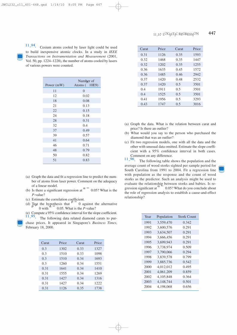
11-10 LOGISTIC REGRESSION 447
Carat Price
0.3 13020.3 15100.3 15100.3 12600.31 16410.31 15550.31 14270.31 14270.31 1126
Carat Price
0.33 13270.33 10980.34 16930.34 15510.34 14100.34 12690.34 13160.34 12220.35 1738
Number ofPower (mW) Atoms (ϫ10E9)
11 012 0.0218 0.0821 0.1322 0.1524 0.1828 0.3132 0.437 0.4939 0.5741 0.6446 0.7148 0.7950 0.8251 0.83
Year Population Stork Count
1991 3,559,470 0.3421992 3,600,576 0.2911993 3,634,507 0.2911994 3,666,456 0.2911995 3,699,943 0.2911996 3,738,974 0.5091997 3,790,066 0.2941998 3,839,578 0.7991999 3,885,736 0.5422000 4,012,012 0.4952001 4,061,209 0.8592002 4,105,848 0.3642003 4,148,744 0.5012004 4,198,068 0.656
(a) Graph the data and fit a regression line to predict the num-ber of atoms from laser power. Comment on the adequacyof a linear model.
(b) Is there a significant regression at ? What is theP-value?
(c) Estimate the correlation coefficient.(d) Test the hypothesis that against the alternative
with . What is the P-value?(e) Compute a 95% confidence interval for the slope coefficient.11-95. The following data related diamond carats to pur-chase prices. It appeared in Singapore’s Business Times,February 18, 2000.
␣ ϭ 0.05 � 0 ϭ 0
␣ ϭ 0.05
(a) Graph the data. What is the relation between carat andprice? Is there an outlier?
(b) What would you say to the person who purchased thediamond that was an outlier?
(c) Fit two regression models, one with all the data and theother with unusual data omitted. Estimate the slope coeffi-cient with a 95% confidence interval in both cases.Comment on any difference.
11-96. The following table shows the population and theaverage count of wood storks sighted per sample period forSouth Carolina from 1991 to 2004. Fit a regression linewith population as the response and the count of woodstorks as the predictor. Such an analysis might be used toevaluate the relationship between storks and babies. Is re-gression significant at ? What do you conclude aboutthe role of regression analysis to establish a cause-and-effectrelationship?
␣ ϭ 0.05
Carat Price
0.31 11260.32 14680.32 12020.36 16350.36 14850.37 14200.37 14200.4 19110.4 15250.41 19560.43 1747
Carat Price
0.35 15930.35 14470.35 12550.45 15720.46 29420.48 25320.5 35010.5 35010.5 35010.5 32930.5 3016
11-94. Cesium atoms cooled by laser light could be usedto build inexpensive atomic clocks. In a study in IEEETransactions on Instrumentation and Measurement (2001,Vol. 50, pp. 1224–1228), the number of atoms cooled by lasersof various powers were counted.
JWCL232_c11_401-448.qxd 1/14/10 8:05 PM Page 447

448 CHAPTER 11 SIMPLE LINEAR REGRESSION AND CORRELATION
IMPORTANT TERMS AND CONCEPTS
Analysis of variance
test in regression
Confidence interval
on mean response
Correlation
coefficient
Empirical model
Confidence intervals on
model parameters
Intrinsically linear model
Least squares estimation
of regression model
parameters
Logistic regression
Model adequacy checking
Odds ratio
Prediction interval on a
future observation
Regression analysis
Residual plots
Residuals
Scatter diagram
Significance of regression
Simple linear regression
model standard errors
Statistical tests on
model parameters
Transformations
MIND-EXPANDING EXERCISES
11-97. Suppose that we have n pairs of observations(xi, yi) such that the sample correlation coefficient r isunity (approximately). Now let zi ϭ y2
i and consider thesample correlation coefficient for the n-pairs of data(xi, zi). Will this sample correlation coefficient be ap-proximately unity? Explain why or why not.11-98. Consider the simple linear regression model Y ϭ 0 ϩ 1x ϩ ⑀, with E(⑀) ϭ 0, V(⑀) ϭ 2, and theerrors ⑀ uncorrelated.(a) Show that cov(b) Show that cov .11-99. Consider the simple linear regression model Y ϭ 0 ϩ 1x ϩ ⑀, with E(⑀) ϭ 0, V(⑀) ϭ 2, and theerrors ⑀ uncorrelated.(a) Show that E( ) ϭ E(MSE) ϭ 2.(b) Show that E(MSR) ϭ 2 ϩ 1
2Sx x.11-100. Suppose that we have assumed the straight-line regression model
but the response is affected by a second variable x2 suchthat the true regression function is
Is the estimator of the slope in the simple linear regres-sion model unbiased?11-101. Suppose that we are fitting a line and wewish to make the variance of the regression coefficient
as small as possible. Where should the observationsxi, i ϭ 1, 2, p , n, be taken so as to minimize V( )?Discuss the practical implications of this allocation ofthe xi.11-102. Weighted Least Squares. Suppose that weare fitting the line Y ϭ 0 ϩ 1x ϩ ⑀, but the variance
1
1
E1Y 2 ϭ 0 ϩ 1x1 ϩ 2x2
Y ϭ 0 ϩ 1x1 ϩ ⑀
2
1Y, 12 ϭ 010, 12 ϭ Ϫx2րSx x.
of Y depends on the level of x; that is,
where the wi are constants, often called weights. Showthat for an objective function in which each squaredresidual is multiplied by the reciprocal of the variance ofthe corresponding observation, the resulting weightedleast squares normal equations are
Find the solution to these normal equations. The solutionsare weighted least squares estimators of 0 and 1.11-103. Consider a situation where both Y and X arerandom variables. Let sx and sy be the sample standarddeviations of the observed x’s and y’s, respectively.Show that an alternative expression for the fitted simplelinear regression model is
11-104. Suppose that we are interested in fitting asimple linear regression model Y ϭ 0 ϩ 1x ϩ ⑀,where the intercept, 0, is known.(a) Find the least squares estimator of 1.(b) What is the variance of the estimator of the slope in
part (a)?(c) Find an expression for a 100(1 Ϫ ␣)% confidence in-
terval for the slope 1. Is this interval longer than thecorresponding interval for the case where both the in-tercept and slope are unknown? Justify your answer.
y ϭ y ϩ rsy
sx1x Ϫ x 2
y ϭ 0 ϩ 1x
0an
iϭ1wixi ϩ 1a
n
iϭ1wixi
2 ϭ an
iϭ1wixi yi
0an
iϭ1wi ϩ 1a
n
iϭ1wixi ϭ a
n
iϭ1wi yi
V1Yi 0 xi2 ϭ 2i ϭ
2
wi i ϭ 1, 2, p , n
JWCL232_c11_401-448.qxd 1/14/10 8:05 PM Page 448

449
12Multiple Linear Regression
This chapter generalizes the simple linear regression to a situation where there is morethan one predictor or regressor variable. This situation occurs frequently in science andengineering; for example, in Chapter 1 we provided data on the pull strength of a wirebond on a semiconductor package and illustrated its relationship to the wire length andthe die height. Understanding the relationship between strength and the other two vari-ables may provide important insight to the engineer when the package is designed, or tothe manufacturing personnel who assemble the die into the package. We used a multiplelinear regression model to relate strength to wire length and die height. There are manyexamples of such relationships: The life of a cutting tool is related to the cutting speed andthe tool angle; patient satisfaction in a hospital is related to patient age, type of procedureperformed, and length of stay; and the fuel economy of a vehicle is related to the type ofvehicle (car versus truck), engine displacement, horsepower, type of transmission, andvehicle weight. Multiple regression models give insight into the relationships betweenthese variables that can have important practical implications.
This chapter shows how to fit multiple linear regression models, perform the statis-tical tests and confidence procedures that are analogous to those for simple linearregression, and check for model adequacy. We also show how models that have polyno-mial terms in the regressor variables are just multiple linear regression models. We alsodiscuss some aspects of building a good regression model from a collection of candidateregressors.
CHAPTER OUTLINE
12-1 MULTIPLE LINEAR REGRESSION
MODEL
12-1.1 Introduction
12-1.2 Least Squares Estimation of
the Parameters
12-1.3 Matrix Approach to Multiple
Linear Regression
12-1.4 Properties of the Least Squares
Estimators
© David Lewis/iStockphoto
JWCL232_c12_449-512.qxd 1/16/10 10:43 AM Page 449

450 CHAPTER 12 MULTIPLE LINEAR REGRESSION
LEARNING OBJECTIVES
After careful study of this chapter you should be able to do the following:
1. Use multiple regression techniques to build empirical models to engineering and scientific
data
2. Understand how the method of least squares extends to fitting multiple regression models
3. Assess regression model adequacy
4. Test hypotheses and construct confidence intervals on the regression coefficients
5. Use the regression model to estimate the mean response and to make predictions and to construct
confidence intervals and prediction intervals
6. Build regression models with polynomial terms
7. Use indicator variables to model categorical regressors
8. Use stepwise regression and other model building techniques to select the appropriate set of vari-
ables for a regression model
12-1 MULTIPLE LINEAR REGRESSION MODEL
12-1.1 Introduction
Many applications of regression analysis involve situations in which there are more than oneregressor or predictor variable. A regression model that contains more than one regressor vari-able is called a multiple regression model.
As an example, suppose that the effective life of a cutting tool depends on the cutting speedand the tool angle. A multiple regression model that might describe this relationship is
(12-1)
where Y represents the tool life, x1 represents the cutting speed, x2 represents the tool angle,and ⑀ is a random error term. This is a multiple linear regression model with two regressors.The term linear is used because Equation 12-1 is a linear function of the unknown parameters0, 1, and 2.
Y ϭ 0 ϩ 1x1 ϩ 2x2 ϩ ⑀
12-2 HYPOTHESIS TESTS IN MULTIPLE
LINEAR REGRESSION
12-2.1 Test for Significance of
Regression
12-2.2 Tests on Individual Regression
Coefficients and Subsets of
Coefficients
12-3 CONFIDENCE INTERVALS
IN MULTIPLE LINEAR
REGRESSION
12-3.1 Confidence Intervals on
Individual Regression
Coefficients
12-3.2 Confidence Interval on
the Mean Response
12-4 PREDICTION OF NEW
OBSERVATIONS
12-5 MODEL ADEQUACY CHECKING
12-5.1 Residual Analysis
12-5.2 Influential Observations
12-6 ASPECTS OF MULTIPLE
REGRESSION MODELING
12-6.1 Polynomial Regression Models
12-6.2 Categorical Regressors and
Indicator Variables
12-6.3 Selection of Variables and
Model Building
12-6.4 Multicollinearity
JWCL232_c12_449-512.qxd 1/15/10 10:06 PM Page 450

12-1 MULTIPLE LINEAR REGRESSION MODEL 451
The regression model in Equation 12-1 describes a plane in the three-dimensional spaceof Y, x1, and x2. Figure 12-1(a) shows this plane for the regression model
where we have assumed that the expected value of the error term is zero; that is E(⑀) ϭ 0. Theparameter 0 is the intercept of the plane. We sometimes call 1 and 2 partial regressioncoefficients, because 1 measures the expected change in Y per unit change in x1 when x2 isheld constant, and 2 measures the expected change in Y per unit change in x2 when x1 is heldconstant. Figure 12-1(b) shows a contour plot of the regression model—that is, lines of con-stant E(Y ) as a function of x1 and x2. Notice that the contour lines in this plot are straight lines.
In general, the dependent variable or response Y may be related to k independent orregressor variables. The model
(12-2)
is called a multiple linear regression model with k regressor variables. The parameters j,j ϭ 0, 1, p , k, are called the regression coefficients. This model describes a hyperplane in the k-dimensional space of the regressor variables {xj}. The parameter j represents theexpected change in response Y per unit change in xj when all the remaining regressors xi (i � j)are held constant.
Multiple linear regression models are often used as approximating functions. That is, thetrue functional relationship between Y and x1, x2, p , xk is unknown, but over certain rangesof the independent variables the linear regression model is an adequate approximation.
Models that are more complex in structure than Equation 12-2 may often still be analyzedby multiple linear regression techniques. For example, consider the cubic polynomial modelin one regressor variable.
(12-3)
If we let x1 ϭ x, x2 ϭ x2, x3 ϭ x3, Equation 12-3 can be written as
(12-4)
which is a multiple linear regression model with three regressor variables.
Y ϭ 0 ϩ 1x1 ϩ 2x2 ϩ 3x3 ϩ ⑀
Y ϭ 0 ϩ 1x ϩ 2x2 ϩ 3x3 ϩ ⑀
Y ϭ 0 ϩ 1x1 ϩ 2x2 ϩ p ϩ ˛kx˛k ϩ ⑀
E1Y 2 ϭ 50 ϩ 10x1 ϩ 7x2
Figure 12-1 (a) The regression plane for the model E(Y ) ϭ 50 ϩ 10x1 ϩ 7x2. (b) The contour plot.
00
2
2 4 6 8 10
(b)
x1
2
4
6
8
10
x2
46
810
8 10 06420
0
40
80
120
160
200
240
(a)
x1
x2
E(Y)
220
203
186
169
1521351181018467
JWCL232_c12_449-512.qxd 1/15/10 10:07 PM Page 451

452 CHAPTER 12 MULTIPLE LINEAR REGRESSION
Models that include interaction effects may also be analyzed by multiple linear regres-sion methods. An interaction between two variables can be represented by a cross-productterm in the model, such as
(12-5)
If we let x3 ϭ x1x2 and 3 ϭ 12, Equation 12-5 can be written as
which is a linear regression model.Figure 12-2(a) and (b) shows the three-dimensional plot of the regression model
and the corresponding two-dimensional contour plot. Notice that, although this model is alinear regression model, the shape of the surface that is generated by the model is not linear.In general, any regression model that is linear in parameters (the ’s) is a linear regressionmodel, regardless of the shape of the surface that it generates.
Figure 12-2 provides a nice graphical interpretation of an interaction. Generally, interactionimplies that the effect produced by changing one variable (x1, say) depends on the level of theother variable (x2). For example, Fig. 12-2 shows that changing x1 from 2 to 8 produces a muchsmaller change in E(Y ) when x2 ϭ 2 than when x2 ϭ 10. Interaction effects occur frequently inthe study and analysis of real-world systems, and regression methods are one of the techniquesthat we can use to describe them.
As a final example, consider the second-order model with interaction
(12-6)
If we let x3 ϭ x21, x4 ϭ x2
2, x5 ϭ x1x2, 3 ϭ 11, 4 ϭ 22, and 5 ϭ 12, Equation 12-6 can bewritten as a multiple linear regression model as follows:
Figure 12-3(a) and (b) show the three-dimensional plot and the corresponding contour plot for
These plots indicate that the expected change in Y when x1 is changed by one unit (say) is afunction of both x1 and x2. The quadratic and interaction terms in this model produce a mound-shaped function. Depending on the values of the regression coefficients, the second-ordermodel with interaction is capable of assuming a wide variety of shapes; thus, it is a veryflexible regression model.
12-1.2 Least Squares Estimation of the Parameters
The method of least squares may be used to estimate the regression coefficients in the mul-tiple regression model, Equation 12-2. Suppose that n Ͼ k observations are available, and let
E1Y 2 ϭ 800 ϩ 10x1 ϩ 7x2 Ϫ 8.5x21 Ϫ 5x2
2 ϩ 4x˛1x2
Y ϭ 0 ϩ 1x1 ϩ 2x2 ϩ 3x3 ϩ 4x4 ϩ 5x5 ϩ ⑀
Y ϭ 0 ϩ 1x1 ϩ 2x2 ϩ 11x21 ϩ 22x2
2 ϩ 12x1x2 ϩ ⑀
Y ϭ 50 ϩ 10x1 ϩ 7x2 ϩ 5x1x2
Y ϭ 0 ϩ 1x1 ϩ 2x2 ϩ 3x3 ϩ ⑀
Y ϭ 0 ϩ 1x1 ϩ 2x2 ϩ 12x1x2 ϩ ⑀
JWCL232_c12_449-512.qxd 1/15/10 10:07 PM Page 452

12-1 MULTIPLE LINEAR REGRESSION MODEL 453
xij denote the ith observation or level of variable xj. The observations are
It is customary to present the data for multiple regression in a table such as Table 12-1.Each observation (xi1, xi2, p , xik, yi), satisfies the model in Equation 12-2, or
(12-7)ϭ 0 ϩak
jϭ1j xij ϩ ⑀i i ϭ 1,˛ 2, p , ˛n
y˛i ϭ 0 ϩ 1xi1 ϩ 2xi 2 ϩ p ϩ k xik ϩ ⑀i
1xi 1, ˛xi 2, p , xik, ˛yi2, i ϭ 1, 2, p , ˛n and n Ͼ k
Figure 12-2 (a) Three-dimensional plot of the regression modelE(Y ) ϭ 50 ϩ 10x1 ϩ 7x2 ϩ 5x1x2. (b) The contour plot.
Figure 12-3 (a) Three-dimensional plot of the regressionmodel E(Y ) ϭ 800 ϩ 10x1 ϩ 7x2 Ϫ 8.5x2
1 Ϫ 5x22 ϩ 4x1x2.
(b) The contour plot.
24
68
10
810
06420
0
200
400
600
800
(a)
x1
x2
E(Y)
00
2 4 6 8 10
(b)
x1
2
4
6
8
10
x2
720
586
452
318
184117
653
519
385
251
00
2
2 4 6 8 10
(b)
x1
2
4
6
8
10
x2
46
810
8 10064
200
200
400
800
1000
(a)
x1
x2
E(Y)
25
600
100
175
550625700750800
250325
400475
Table 12-1 Data for Multiple Linear Regression
y x1 x2 . . . xk
y1 x11 x12 . . . x1k
y2 x21 x22 . . . x2k
yn xn1 xn2 . . . xnk
oooo
JWCL232_c12_449-512.qxd 1/15/10 10:07 PM Page 453

The least squares function is
(12-8)
We want to minimize L with respect to 0, 1, p , k. The least squares estimates of 0, 1, p , k must satisfy
(12-9a)
and
(12-9b)
Simplifying Equation 12-9, we obtain the least squares normal equations
(12-10)
Note that there are p ϭ k ϩ 1 normal equations, one for each of the unknown regressioncoefficients. The solution to the normal equations will be the least squares estimators of theregression coefficients, The normal equations can be solved by any methodappropriate for solving a system of linear equations.
0, 1, p , k.
0an
iϭ1˛xik ϩ 1a
n
iϭ1˛xikxi1 ϩ 2 a
n
iϭ1xikxi2 ϩ p ϩ k a
n
iϭ1x2
ik ϭan
iϭ1xikyi
oooooo
0an
iϭ1˛xi1 ϩ 1a
n
iϭ1˛x2
i1 ϩ 2 an
iϭ1xi1 xi2 ϩ p ϩ k a
n
iϭ1xi1xik ϭa
n
iϭ1xi1yi
n0 ϩ 1an
iϭ1˛xi1 ϩ 2˛a
n
iϭ1˛xi 2 ϩ p ϩ ka
n
iϭ1˛xik ϭ a
n
iϭ1˛yi
ѨLѨj`0,1, p , k
ϭ Ϫ2an
iϭ1ayi Ϫ 0 Ϫ a
k
jϭ1jxijb xij ϭ 0 j ϭ 1, 2, p , k
ѨLѨ0`0,1, p , k
ϭ Ϫ2an
iϭ1ayi Ϫ 0 Ϫa
k
jϭ1j xijb ϭ 0
L ϭan
iϭ1˛⑀2
i ϭan
iϭ1˛ayi Ϫ 0 Ϫa
k
jϭ1˛ j xijb2
454 CHAPTER 12 MULTIPLE LINEAR REGRESSION
EXAMPLE 12-1 Wire Bond StrengthIn Chapter 1, we used data on pull strength of a wire bond in asemiconductor manufacturing process, wire length, and dieheight to illustrate building an empirical model. We will usethe same data, repeated for convenience in Table 12-2, andshow the details of estimating the model parameters. A three-dimensional scatter plot of the data is presented in Fig. 1-15.Figure 12-4 shows a matrix of two-dimensional scatter plots ofthe data. These displays can be helpful in visualizing therelationships among variables in a multivariable data set. Forexample, the plot indicates that there is a strong linearrelationship between strength and wire length.
Specifically, we will fit the multiple linear regressionmodel
where Y ϭ pull strength, x1 ϭ wire length, and x2 ϭ dieheight. From the data in Table 12-2 we calculate
Y ϭ 0 ϩ 1x1 ϩ 2x2 ϩ ⑀
a25
iϭ1xi2yi ϭ 274,816.71
a25
iϭ1˛xi1xi2 ϭ 77,177, a
25
iϭ1˛xi1yi ϭ 8,008.47,
a25
iϭ1x2
i1 ϭ 2,396, a25
iϭ1˛x2
i2 ϭ 3,531,848
a25
iϭ1xi1 ϭ 206, a
25
iϭ1˛xi 2 ϭ 8,294
n ϭ 25, a25
iϭ1˛yi ϭ 725.82
JWCL232_c12_449-512.qxd 1/15/10 10:07 PM Page 454

12-1 MULTIPLE LINEAR REGRESSION MODEL 455
For the model Y ϭ 0 ϩ 1x1 ϩ 2x2 ϩ ⑀, the normal equa-tions 12-10 are
0an
iϭ1˛xi 2 ϩ 1a
n
iϭ1˛xi1xi 2 ϩ 2a
n
iϭ1˛x2
i 2 ϭ an
iϭ1˛xi 2 yi
0an
iϭ1˛ xi1 ϩ ˛1a
n
iϭ1˛x2
i1 ϩ 2an
iϭ1˛xi1xi2 ϭ a
n
iϭ1xi1˛yi
n0 ϩ 1an
iϭ1˛xi1 ϩ 2a
n
iϭ1˛xi 2 ϭ a
n
iϭ1yi
Inserting the computed summations into the normal equa-tions, we obtain
82940 ϩ 77,1771 ϩ 3,531,8482 ϭ 274,816.71
2060 ϩ 23961 ϩ 77,1772 ϭ 8,008.47
250 ϩ 2061 ϩ 82942 ϭ 725.82
Table 12-2 Wire Bond Data for Example 12-1
Observation Pull Strength Wire Length Die Height Observation Pull Strength Wire Length Die HeightNumber y x1 x2 Number y x1 x2
1 9.95 2 50 14 11.66 2 360
2 24.45 8 110 15 21.65 4 205
3 31.75 11 120 16 17.89 4 400
4 35.00 10 550 17 69.00 20 600
5 25.02 8 295 18 10.30 1 585
6 16.86 4 200 19 34.93 10 540
7 14.38 2 375 20 46.59 15 250
8 9.60 2 52 21 44.88 15 290
9 24.35 9 100 22 54.12 16 510
10 27.50 8 300 23 56.63 17 590
11 17.08 4 412 24 22.13 6 100
12 37.00 11 400 25 21.15 5 40013 41.95 12 500
Figure 12-4 Matrix of scatter plots (from Minitab) for the wire bond pullstrength data in Table 12-2.
187.5
24.45 54.15
462.5
5.75 15.25 187.5 462.5
Strength
Length
Height
5.75
15.25
24.45
54.15
JWCL232_c12_449-512.qxd 1/15/10 10:07 PM Page 455

12-1.3 Matrix Approach to Multiple Linear Regression
In fitting a multiple regression model, it is much more convenient to express the mathemati-cal operations using matrix notation. Suppose that there are k regressor variables and n ob-servations, (xi1, xi2, p , xik, yi), i ϭ 1, 2, p , n and that the model relating the regressors to theresponse is
This model is a system of n equations that can be expressed in matrix notation as
y ؍ X � ⑀ (12-11)where
and ⑀
In general, y is an (n ϫ 1) vector of the observations, X is an (n ϫ p) matrix of the levelsof the independent variables (assuming that the intercept is always multiplied by a constantvalue—unity),  is a ( p ϫ 1) vector of the regression coefficients, and ⑀ is a (n ϫ 1) vectorof random errors. The X matrix is often called the model matrix.
We wish to find the vector of least squares estimators, , that minimizes
The least squares estimator  is the solution for  in the equations
We will not give the details of taking the derivatives above; however, the resulting equationsthat must be solved are
ѨLѨ
ϭ 0
L ϭ an
iϭ1˛⑀2
i ϭ ⑀¿⑀ ϭ 1y Ϫ X2 ¿ 1y Ϫ X2
؍ ≥ ⑀1
⑀2
o
⑀n
¥ ؍ ≥ 0
1
o
k
¥X ؍ ≥ 1 x11 x12 p x1k
1 x21 x22 p x2k
o o o o
1 xn1 xn2 p xnk
¥y ؍ ≥ y1
y2
o
yn
¥
yi ϭ 0 ϩ 1xi1 ϩ 2xi 2 ϩ p ϩ kxik ϩ ⑀i i ϭ 1, 2, p , n
456 CHAPTER 12 MULTIPLE LINEAR REGRESSION
The solution to this set of equations is
Therefore, the fitted regression equation is
y ϭ 2.26379 ϩ 2.74427x1 ϩ 0.01253x2
0 ϭ 2.26379, 1 ϭ 2.74427, 2 ϭ 0.01253
Practical Interpretation: This equation can be used topredict pull strength for pairs of values of the regressor vari-ables wire length (x1) and die height (x2). This is essentiallythe same regression model given in Section 1-3. Figure 1-16shows a three-dimensional plot of the plane of predicted val-ues generated from this equation.y
XX ؍ Xy (12-12)Normal
Equations
JWCL232_c12_449-512.qxd 1/15/10 10:07 PM Page 456

12-1 MULTIPLE LINEAR REGRESSION MODEL 457
Note that there are p ϭ k ϩ 1 normal equations in p ϭ k ϩ 1 unknowns (the values ofFurthermore, the matrix XX is always nonsingular, as was assumed above,
so the methods described in textbooks on determinants and matrices for inverting these ma-trices can be used to find . In practice, multiple regression calculations are almost always performed using a computer.
It is easy to see that the matrix form of the normal equations is identical to the scalar form.Writing out Equation 12-12 in detail, we obtain
If the indicated matrix multiplication is performed, the scalar form of the normal equations(that is, Equation 12-10) will result. In this form it is easy to see that is a ( p ϫ p) sym-metric matrix and is a ( p ϫ 1) column vector. Note the special structure of the ma-trix. The diagonal elements of are the sums of squares of the elements in the columns ofX, and the off-diagonal elements are the sums of cross-products of the elements in thecolumns of X. Furthermore, note that the elements of are the sums of cross-products ofthe columns of X and the observations
The fitted regression model is
(12-14)
In matrix notation, the fitted model is
The difference between the observation yi and the fitted value is a residual, say,The (n ϫ 1) vector of residuals is denoted by
(12-15)e ϭ y Ϫ y
ei ϭ yi Ϫ yi.yi
y ϭ X
yi ϭ 0 ϩ ak
jϭ1˛j ˛xi j i ϭ 1, ˛2, p ,˛ n
5yi6. Xy
XXXXXy
XX
H0
1
o
k
X ϭ H aniϭ1yi
an
iϭ1xi1yi
o
an
iϭ1xik˛ yi
XH n an
iϭ1xi1 a
n
iϭ1xi2
p an
iϭ1xik
an
iϭ1xi1 a
n
iϭ1x2
i1 an
iϭ1xi1xi2
p an
iϭ1xi1xik
o o o o
an
iϭ1xik a
n
iϭ1xik xi1 a
n
iϭ1xik xi2
p an
iϭ1x2
ik
X1X¿X2Ϫ1
0, 1, p , k2.
Equations 12-12 are the least squares normal equations in matrix form. They are identical tothe scalar form of the normal equations given earlier in Equations 12-10. To solve the normalequations, multiply both sides of Equations 12-12 by the inverse of Therefore, the leastsquares estimate of  is
X¿X.
 ؍ (XX)�1 Xy (12-13)Least SquareEstimate of �
JWCL232_c12_449-512.qxd 1/15/10 10:07 PM Page 457

458 CHAPTER 12 MULTIPLE LINEAR REGRESSION
EXAMPLE 12-2 Wire Bond Strength with Matrix NotationIn Example 12-1, we illustrated fitting the multiple regressionmodel
where y is the observed pull strength for a wire bond, x1 is thewire length, and x2 is the die height. The 25 observations are inTable 12-2. We will now use the matrix approach to fit the re-gression model above to these data. The model matrix X and yvector for this model are
X ϭ y ϭ
The matrix is
ϭ £ 25 206 8,294206 2,396 77,177
8,294 77,177 3,531,848§
X¿X ϭ £ 1 1 p 12 8 p 5
50 110 p 400§ ˛ ≥ 1 2 50
1 8 110o o o
1 5 400
¥X¿X
9.9524.4531.7535.0025.0216.8614.389.60
24.3527.5017.0837.0041.9511.6621.6517.8969.0010.3034.9346.5944.8854.1256.6322.1321.15
1 2 501 8 1101 11 1201 10 5501 8 2951 4 2001 2 3751 2 521 9 1001 8 3001 4 4121 11 4001 12 5001 2 3601 4 2051 4 4001 20 6001 1 5851 10 5401 15 2501 15 2901 16 5101 17 5901 6 1001 5 400
y ϭ 0 ϩ 1˛x1 ϩ 2x2 ϩ ⑀
and the vector is
The least squares estimates are found from Equation 12-13 as
 ؍ (XX)�1Xy
or
Therefore, the fitted regression model with the regressioncoefficients rounded to five decimal places is
This is identical to the results obtained in Example 12-1.This regression model can be used to predict values of
pull strength for various values of wire length (x1) and dieheight (x2). We can also obtain the fitted values by substi-tuting each observation (xi1, xi2), i ϭ 1, 2, . . . , n, into theequation. For example, the first observation has x11 ϭ 2 andx12 ϭ 50, and the fitted value is
The corresponding observed value is y1 ϭ 9.95. The residualcorresponding to the first observation is
Table 12-3 displays all 25 fitted values and the correspon-ding residuals. The fitted values and residuals are calculated tothe same accuracy as the original data.
yi
ϭ 1.57ϭ 9.95 Ϫ 8.38
e1 ϭ y1 Ϫ y1
ϭ 8.38ϭ 2.26379 ϩ 2.74427122 ϩ 0.012531502y1 ϭ 2.26379 ϩ 2.74427x11 ϩ 0.01253x12
yi
y ϭ 2.26379 ϩ 2.74427x1 ϩ 0.01253x2
ϭ £ 2.263791432.744269640.01252781
§£ 725.82
8,008.47274,811.31
§ϭ £ 0.214653 Ϫ0.007491 Ϫ0.000340Ϫ0.007491 0.001671 Ϫ0.000019Ϫ0.000340 Ϫ0.000019 ϩ0.0000015
§£ 0
1
2
§ ϭ £ 25 206 8,294206 2,396 77,177
8,294 77,177 3,531,848§ Ϫ1 £ 725.82
8,008.37274,811.31
§
X¿y ϭ £ 1 1 p 12 8 p 5
50 110 p 400§ ≥ 9.95
24.45o
21.15
¥ ϭ £ 725.828,008.47
274,816.71§
X¿y
JWCL232_c12_449-512.qxd 1/15/10 10:07 PM Page 458

12-1 MULTIPLE LINEAR REGRESSION MODEL 459
Computers are almost always used in fitting multiple regression models. Table 12-4 pre-sents some annotated output from Minitab for the least squares regression model for wire bondpull strength data. The upper part of the table contains the numerical estimates of the regres-sion coefficients. The computer also calculates several other quantities that reflect importantinformation about the regression model. In subsequent sections, we will define and explain thequantities in this output.
Estimating �2
Just as in simple linear regression, it is important to estimate 2, the variance of the error term⑀, in a multiple regression model. Recall that in simple linear regression the estimate of 2 wasobtained by dividing the sum of the squared residuals by n Ϫ 2. Now there are two parame-ters in the simple linear regression model, so in multiple linear regression with p parameters alogical estimator for 2 is
This is an unbiased estimator of 2. Just as in simple linear regression, the estimate of 2 is usu-ally obtained from the analysis of variance for the regression model. The numerator of Equation12-16 is called the error or residual sum of squares, and the denominator n Ϫ p is called the error or residual degrees of freedom.
We can find a computing formula for SSE as follows:
Substituting into the above, we obtain
(12-17)ϭ 27,178.5316 Ϫ 27,063.3581 ϭ 115.174SSE ϭ y¿y Ϫ ¿X¿y
e ϭ y Ϫ y ϭ y Ϫ X
SSE ϭ an
iϭ11 yi Ϫ yi22 ϭ a
n
iϭ1ei
2 ϭ e¿e
Table 12-3 Observations, Fitted Values, and Residuals for Example 12-2
Observation Number
1 9.95 8.38 1.572 24.45 25.60 Ϫ1.153 31.75 33.95 Ϫ2.204 35.00 36.60 Ϫ1.605 25.02 27.91 Ϫ2.896 16.86 15.75 1.117 14.38 12.45 1.938 9.60 8.40 1.209 24.35 28.21 Ϫ3.86
10 27.50 27.98 Ϫ0.4811 17.08 18.40 Ϫ1.3212 37.00 37.46 Ϫ0.4613 41.95 41.46 0.49
ei ϭ yi Ϫ yiyiyi
14 11.66 12.26 Ϫ0.6015 21.65 15.81 5.8416 17.89 18.25 Ϫ0.3617 69.00 64.67 4.3318 10.30 12.34 Ϫ2.0419 34.93 36.47 Ϫ1.5420 46.59 46.56 0.0321 44.88 47.06 Ϫ2.1822 54.12 52.56 1.5623 56.63 56.31 0.3224 22.13 19.98 2.1525 21.15 21.00 0.15
Observation Number ei ϭ yi Ϫ yiyiyi
(12-16)2 ϭa
n
iϭ1˛e2
i
n Ϫ p ϭSSE
n Ϫ p
Estimator of Variance
JWCL232_c12_449-512.qxd 1/15/10 10:07 PM Page 459

460 CHAPTER 12 MULTIPLE LINEAR REGRESSION
Table 12-4 shows that the estimate of 2 for the wire bond pull strength regression modelis 2 ϭ 115.222 ϭ 5.2364. The Minitab output rounds the estimate to 2 ϭ 5.2.
12-1.4 Properties of the Least Squares Estimators
The statistical properties of the least squares estimators may be easily found,under certain assumptions on the error terms ⑀1, ⑀2, p , ⑀n, in the regression model. Parallelingthe assumptions made in Chapter 11, we assume that the errors ⑀i are statistically independentwith mean zero and variance 2. Under these assumptions, the least squares estimators
are unbiased estimators of the regression coefficients 0, 1, p , k. Thisproperty may be shown as follows:
since E(⑀) ؍ 0 and (XЈX)Ϫ1XЈX ؍ I, the identity matrix. Thus, is an unbiased estimator of .
ϭ 
ϭ E 3 1X¿X2Ϫ1X¿X ϩ 1X¿X2Ϫ1X¿⑀ 4ϭ E 3 1X¿X2Ϫ1X¿ 1X ϩ ⑀2 4E12 ϭ E 3 1X¿X2Ϫ1X¿Y 40, 1, p ,˛ k
0, 1, p , k
Table 12-4 Minitab Multiple Regression Output for the Wire Bond Pull Strength Data
Regression Analysis: Strength versus Length, Height
The regression equation isStrength ϭ 2.26 ϩ 2.74 Length ϩ 0.0125 Height
Predictor Coef SE Coef T P VIFConstant 0 2.264 1.060 2.14 0.044Length 1 2.74427 0.09352 29.34 0.000 1.2Height 2 0.012528 0.002798 4.48 0.000 1.2
S ϭ 2.288 R-Sq ϭ 98.1% R-Sq (adj) ϭ 97.9%PRESS ϭ 156.163 R-Sq (pred) ϭ 97.44%
Analysis of Variance
Source DF SS MS F PRegression 2 5990.8 2995.4 572.17 0.000Residual Error 22 115.2 5.2Total 24 6105.9
Source DF Seq SSLength 1 5885.9Height 1 104.9
Predicted Values for New Observations
New Obs Fit SE Fit 95.0% CI 95.0% PI1 27.663 0.482 (26.663, 28.663) (22.814, 32.512)
Values of Predictors for New Observations
New Obs Length Height1 8.00 275
2
JWCL232_c12_449-512.qxd 1/15/10 10:07 PM Page 460

12-1 MULTIPLE LINEAR REGRESSION MODEL 461
The variances of the ’s are expressed in terms of the elements of the inverse of the matrix. The inverse of times the constant 2 represents the covariance matrix of theregression coefficients . The diagonal elements of are the variances of
and the off-diagonal elements of this matrix are the covariances. For example, if wehave k ϭ 2 regressors, such as in the pull-strength problem,
which is symmetric (C10 ϭ C01, C20 ϭ C02, and C21 ϭ C12) because (XЈX)Ϫ1 is symmetric,and we have
In general, the covariance matrix of is a ( p ϫ p) symmetric matrix whose jjth element is the variance of and whose i, jth element is the covariance between and that is,
The estimates of the variances of these regression coefficients are obtained by replacing2 with an estimate. When 2 is replaced by its estimate , the square root of the estimated variance of the jth regression coefficient is called the estimated standard error of or
These standard errors are a useful measure of the precision of estimationfor the regression coefficients; small standard errors imply good precision.
Multiple regression computer programs usually display these standard errors. Forexample, the Minitab output in Table 12-4 reports and
The intercept estimate is about twice the magnitude of its standard error, andare considerably larger than and This implies reasonable precision
of estimation, although the parameters 1 and 2 are much more precisely estimated than theintercept (this is not unusual in multiple regression).
se 122.se 1121 and 2ˆ
se122 ϭ 0.002798.se 102 ϭ 1.060, se 112 ϭ 0.09352,
se 1j2 ϭ 22Cjj.j
2
cov12 ϭ 21X¿X2Ϫ1 ϭ 2C
j,ij

cov1i, j2 ϭ 2C˛ij, i � j
V 1˛j2 ϭ 2C˛jj, j ϭ 0, 1, 2
C ϭ 1X¿X2Ϫ1 ϭ £C00 C01 C02
C10 C11 C12
C20 C21 C22
§1, p , k,
0,2 1X¿X2Ϫ1
X¿XX¿X
12-1. A study was performed to investigate the shearstrength of soil ( y) as it related to depth in feet (x1) and %moisture content (x2). Ten observations were collected, and thefollowing summary quantities obtained: n ϭ 10,
and (a) Set up the least squares normal equations for the model
Y ϭ 0 ϩ 1x1 ϩ 2x2 ϩ ⑀.(b) Estimate the parameters in the model in part (a).(c) What is the predicted strength when x1 ϭ 18 feet and
x2 ϭ 43%?12-2. A regression model is to be developed for predictingthe ability of soil to absorb chemical contaminants. Ten obser-vations have been taken on a soil absorption index ( y) and tworegressors: x1 ϭ amount of extractable iron ore and x2 ϭ
gy2i ϭ 371,595.6.
gxi2 yi ϭ 104,736.8,gxi1 yi ϭ 43,550.8,gxi1xi2 ϭ 12,352,gx2
i2 ϭ 31,729,gx2i1 ϭ 5,200.9,gyi ϭ 1,916,gxi2 ϭ 553,
gxi1 ϭ 223,
amount of bauxite. We wish to fit the model Y ϭ 0 ϩ 1x1 ϩ
2x2 ϩ ⑀. Some necessary quantities are:
(a) Estimate the regression coefficients in the model specifiedabove.
(b) What is the predicted value of the absorption index ywhen x1 ϭ 200 and x2 ϭ 50?
12-3. A chemical engineer is investigating how the amountof conversion of a product from a raw material (y) depends on
Xy ϭ £ 22036,7689,965
§1XX2Ϫ1 ϭ
1.17991 Ϫ7.30982 E-3 7.3006 E-4£Ϫ7.30982 E-3 7.9799 E-5 Ϫ1.23713 E-47.3006 E-4 Ϫ1.23713 E-4 4.6576 E-4
§ ,
EXERCISES FOR SECTION 12-1
JWCL232_c12_449-512.qxd 1/16/10 10:47 AM Page 461
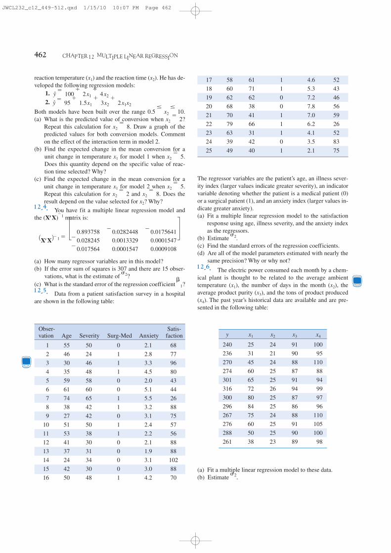
462 CHAPTER 12 MULTIPLE LINEAR REGRESSION
reaction temperature (x1) and the reaction time (x2). He has de-veloped the following regression models:
1.2.
Both models have been built over the range 0.5 Յ x2 Յ 10.(a) What is the predicted value of conversion when x2 ϭ 2?
Repeat this calculation for x2 ϭ 8. Draw a graph of thepredicted values for both conversion models. Commenton the effect of the interaction term in model 2.
(b) Find the expected change in the mean conversion for aunit change in temperature x1 for model 1 when x2 ϭ 5.Does this quantity depend on the specific value of reac-tion time selected? Why?
(c) Find the expected change in the mean conversion for aunit change in temperature x1 for model 2 when x2 ϭ 5.Repeat this calculation for x2 ϭ 2 and x2 ϭ 8. Does theresult depend on the value selected for x2? Why?
12-4. You have fit a multiple linear regression model andthe (X�X)Ϫ1 matrix is:
(a) How many regressor variables are in this model?(b) If the error sum of squares is 307 and there are 15 obser-
vations, what is the estimate of 2?(c) What is the standard error of the regression coefficient ?
12-5. Data from a patient satisfaction survey in a hospitalare shown in the following table:
1
1XX2Ϫ1 ϭ
0.893758 Ϫ0.0282448 Ϫ0.0175641£Ϫ0.028245 0.0013329 0.0001547Ϫ0.017564 0.0001547 0.0009108
§
y ϭ 95 ϩ 1.5x1 ϩ 3x2 ϩ 2x1x2
y ϭ 100 ϩ 2x1 ϩ 4x2
The regressor variables are the patient’s age, an illness sever-ity index (larger values indicate greater severity), an indicatorvariable denoting whether the patient is a medical patient (0)or a surgical patient (1), and an anxiety index (larger values in-dicate greater anxiety).(a) Fit a multiple linear regression model to the satisfaction
response using age, illness severity, and the anxiety indexas the regressors.
(b) Estimate 2.(c) Find the standard errors of the regression coefficients.(d) Are all of the model parameters estimated with nearly the
same precision? Why or why not?
12-6. The electric power consumed each month by a chem-ical plant is thought to be related to the average ambienttemperature (x1), the number of days in the month (x2), theaverage product purity (x3), and the tons of product produced(x4). The past year’s historical data are available and are pre-sented in the following table:
Obser- Satis-vation Age Severity Surg-Med Anxiety faction
1 55 50 0 2.1 682 46 24 1 2.8 773 30 46 1 3.3 964 35 48 1 4.5 805 59 58 0 2.0 436 61 60 0 5.1 447 74 65 1 5.5 268 38 42 1 3.2 889 27 42 0 3.1 75
10 51 50 1 2.4 5711 53 38 1 2.2 5612 41 30 0 2.1 8813 37 31 0 1.9 8814 24 34 0 3.1 10215 42 30 0 3.0 8816 50 48 1 4.2 70
17 58 61 1 4.6 5218 60 71 1 5.3 4319 62 62 0 7.2 4620 68 38 0 7.8 5621 70 41 1 7.0 5922 79 66 1 6.2 2623 63 31 1 4.1 5224 39 42 0 3.5 8325 49 40 1 2.1 75
y x1 x2 x3 x4
240 25 24 91 100236 31 21 90 95270 45 24 88 110274 60 25 87 88301 65 25 91 94316 72 26 94 99300 80 25 87 97296 84 25 86 96267 75 24 88 110276 60 25 91 105288 50 25 90 100261 38 23 89 98
(a) Fit a multiple linear regression model to these data.(b) Estimate 2.
JWCL232_c12_449-512.qxd 1/15/10 10:07 PM Page 462

12-1 MULTIPLE LINEAR REGRESSION MODEL 463
Table 12-5 DaimlerChrysler Fuel Economy and Emissions
mfr carline car/truck cid rhp trns drv od etw cmp axle n/v a/c hc co co2 mpg
20 300C/SRT-8 C 215 253 L5 4 2 4500 9.9 3.07 30.9 Y 0.011 0.09 288 30.8
20 CARAVAN 2WD T 201 180 L4 F 2 4500 9.3 2.49 32.3 Y 0.014 0.11 274 32.5
20 CROSSFIRE ROADSTER C 196 168 L5 R 2 3375 10 3.27 37.1 Y 0.001 0.02 250 35.4
20 DAKOTA PICKUP 2WD T 226 210 L4 R 2 4500 9.2 3.55 29.6 Y 0.012 0.04 316 28.1
20 DAKOTA PICKUP 4WD T 226 210 L4 4 2 5000 9.2 3.55 29.6 Y 0.011 0.05 365 24.4
20 DURANGO 2WD T 348 345 L5 R 2 5250 8.6 3.55 27.2 Y 0.023 0.15 367 24.1
20 GRAND CHEROKEE 2WD T 226 210 L4 R 2 4500 9.2 3.07 30.4 Y 0.006 0.09 312 28.5
20 GRAND CHEROKEE 4WD T 348 230 L5 4 2 5000 9 3.07 24.7 Y 0.008 0.11 369 24.2
20 LIBERTY/CHEROKEE 2WD T 148 150 M6 R 2 4000 9.5 4.1 41 Y 0.004 0.41 270 32.8
20 LIBERTY/CHEROKEE 4WD T 226 210 L4 4 2 4250 9.2 3.73 31.2 Y 0.003 0.04 317 28
20 NEON/SRT-4/SX 2.0 C 122 132 L4 F 2 3000 9.8 2.69 39.2 Y 0.003 0.16 214 41.3
20 PACIFICA 2WD T 215 249 L4 F 2 4750 9.9 2.95 35.3 Y 0.022 0.01 295 30
20 PACIFICA AWD T 215 249 L4 4 2 5000 9.9 2.95 35.3 Y 0.024 0.05 314 28.2
20 PT CRUISER T 148 220 L4 F 2 3625 9.5 2.69 37.3 Y 0.002 0.03 260 34.1
20 RAM 1500 PICKUP 2WD T 500 500 M6 R 2 5250 9.6 4.1 22.3 Y 0.01 0.1 474 18.7
20 RAM 1500 PICKUP 4WD T 348 345 L5 4 2 6000 8.6 3.92 29 Y 0 0 0 20.3
20 SEBRING 4-DR C 165 200 L4 F 2 3625 9.7 2.69 36.8 Y 0.011 0.12 252 35.1
20 STRATUS 4-DR C 148 167 L4 F 2 3500 9.5 2.69 36.8 Y 0.002 0.06 233 37.9
20 TOWN & COUNTRY 2WD T 148 150 L4 F 2 4250 9.4 2.69 34.9 Y 0 0.09 262 33.8
20 VIPER CONVERTIBLE C 500 501 M6 R 2 3750 9.6 3.07 19.4 Y 0.007 0.05 342 25.9
20 WRANGLER/TJ 4WD T 148 150 M6 4 2 3625 9.5 3.73 40.1 Y 0.004 0.43 337 26.4
mfr-mfr codecarline-car line name (test vehicle model name)car/truck-‘C’ for passenger vehicle and ‘T’ for truckcid-cubic inch displacement of test vehiclerhp-rated horsepowertrns-transmission codedrv-drive system codeod-overdrive codeetw-equivalent test weight
cmp-compression ratioaxle-axle ration/v-n/v ratio (engine speed versus vehicle speed at 50 mph)a/c-indicates air conditioning simulationhc-HC(hydrocarbon emissions) Test level composite resultsco-CO(carbon monoxide emissions) Test level composite resultsco2-CO2(carbon dioxide emissions) Test level composite resultsmpg-mpg(fuel economy, miles per gallon)
(c) Compute the standard errors of the regression coeffi-cients. Are all of the model parameters estimated with thesame precision? Why or why not?(d) Predict power consumption for a month in which
x2 ϭ 24 days, x3 ϭ 90%, and x4 ϭ 98 tons.
12-7. Table 12-5 provides the highway gasoline mileage testresults for 2005 model year vehicles from DaimlerChrysler. Thefull table of data (available on the book’s Web site) contains thesame data for 2005 models from over 250 vehicles from manymanufacturers (source: Environmental Protection Agency Website www.epa.gov/ otaq/cert/mpg/testcars/database).(a) Fit a multiple linear regression model to these data to esti-
mate gasoline mileage that uses the following regressors:cid, rhp, etw, cmp, axle, n/v.
x1 ϭ 75ЊF,
(b) Estimate and the standard errors of the regression co-efficients.
(c) Predict the gasoline mileage for the first vehicle in thetable.
12-8. The pull strength of a wire bond is an important char-acteristic. The following table gives information on pullstrength ( y), die height (x1), post height (x2), loop height (x3),wire length (x4), bond width on the die (x5), and bond width onthe post (x6).(a) Fit a multiple linear regression model using x2, x3, x4, and
x5 as the regressors.(b) Estimate 2.(c) Find the se( ). How precisely are the regression coeffi-
cients estimated, in your opinion?jˆ
2
JWCL232_c12_449-512.qxd 1/16/10 10:48 AM Page 463
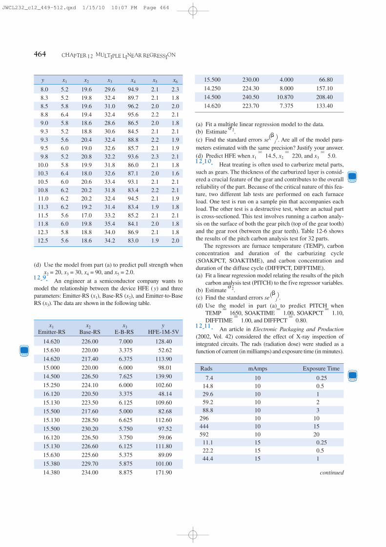
464 CHAPTER 12 MULTIPLE LINEAR REGRESSION
y x1 x2 x3 x4 x5 x6
8.0 5.2 19.6 29.6 94.9 2.1 2.38.3 5.2 19.8 32.4 89.7 2.1 1.88.5 5.8 19.6 31.0 96.2 2.0 2.08.8 6.4 19.4 32.4 95.6 2.2 2.19.0 5.8 18.6 28.6 86.5 2.0 1.89.3 5.2 18.8 30.6 84.5 2.1 2.19.3 5.6 20.4 32.4 88.8 2.2 1.99.5 6.0 19.0 32.6 85.7 2.1 1.99.8 5.2 20.8 32.2 93.6 2.3 2.1
10.0 5.8 19.9 31.8 86.0 2.1 1.810.3 6.4 18.0 32.6 87.1 2.0 1.610.5 6.0 20.6 33.4 93.1 2.1 2.110.8 6.2 20.2 31.8 83.4 2.2 2.111.0 6.2 20.2 32.4 94.5 2.1 1.911.3 6.2 19.2 31.4 83.4 1.9 1.811.5 5.6 17.0 33.2 85.2 2.1 2.111.8 6.0 19.8 35.4 84.1 2.0 1.812.3 5.8 18.8 34.0 86.9 2.1 1.812.5 5.6 18.6 34.2 83.0 1.9 2.0
(d) Use the model from part (a) to predict pull strength whenx2 = 20, x3 = 30, x4 = 90, and x5 = 2.0.
12-9. An engineer at a semiconductor company wants tomodel the relationship between the device HFE ( y) and threeparameters: Emitter-RS (x1), Base-RS (x2), and Emitter-to-BaseRS (x3). The data are shown in the following table.
(a) Fit a multiple linear regression model to the data.(b) Estimate 2.(c) Find the standard errors se Are all of the model para-meters estimated with the same precision? Justify your answer.(d) Predict HFE when x1 ϭ 14.5, x2 ϭ 220, and x3 ϭ 5.0.12-10. Heat treating is often used to carburize metal parts,such as gears. The thickness of the carburized layer is consid-ered a crucial feature of the gear and contributes to the overallreliability of the part. Because of the critical nature of this fea-ture, two different lab tests are performed on each furnaceload. One test is run on a sample pin that accompanies eachload. The other test is a destructive test, where an actual partis cross-sectioned. This test involves running a carbon analy-sis on the surface of both the gear pitch (top of the gear tooth)and the gear root (between the gear teeth). Table 12-6 showsthe results of the pitch carbon analysis test for 32 parts.
The regressors are furnace temperature (TEMP), carbonconcentration and duration of the carburizing cycle(SOAKPCT, SOAKTIME), and carbon concentration andduration of the diffuse cycle (DIFFPCT, DIFFTIME).(a) Fit a linear regression model relating the results of the pitch
carbon analysis test (PITCH) to the five regressor variables.(b) Estimate 2.(c) Find the standard errors (d) Use the model in part (a) to predict PITCH when
TEMP ϭ 1650, SOAKTIME ϭ 1.00, SOAKPCT ϭ 1.10,DIFFTIME ϭ 1.00, and DIFFPCT ϭ 0.80.
12-11. An article in Electronic Packaging and Production(2002, Vol. 42) considered the effect of X-ray inspection ofintegrated circuits. The rads (radiation dose) were studied as afunction of current (in milliamps) and exposure time (in minutes).
se 1jˆ 2.
1jˆ 2.
x1 x2 x3 yEmitter-RS Base-RS E-B-RS HFE-1M-5V
14.620 226.00 7.000 128.4015.630 220.00 3.375 52.6214.620 217.40 6.375 113.9015.000 220.00 6.000 98.0114.500 226.50 7.625 139.9015.250 224.10 6.000 102.6016.120 220.50 3.375 48.1415.130 223.50 6.125 109.6015.500 217.60 5.000 82.6815.130 228.50 6.625 112.6015.500 230.20 5.750 97.5216.120 226.50 3.750 59.0615.130 226.60 6.125 111.8015.630 225.60 5.375 89.0915.380 229.70 5.875 101.0014.380 234.00 8.875 171.90
15.500 230.00 4.000 66.8014.250 224.30 8.000 157.1014.500 240.50 10.870 208.4014.620 223.70 7.375 133.40
Rads mAmps Exposure Time
7.4 10 0.2514.8 10 0.529.6 10 159.2 10 288.8 10 3
296 10 10444 10 15592 10 2011.1 15 0.2522.2 15 0.544.4 15 1
continued
JWCL232_c12_449-512.qxd 1/15/10 10:07 PM Page 464
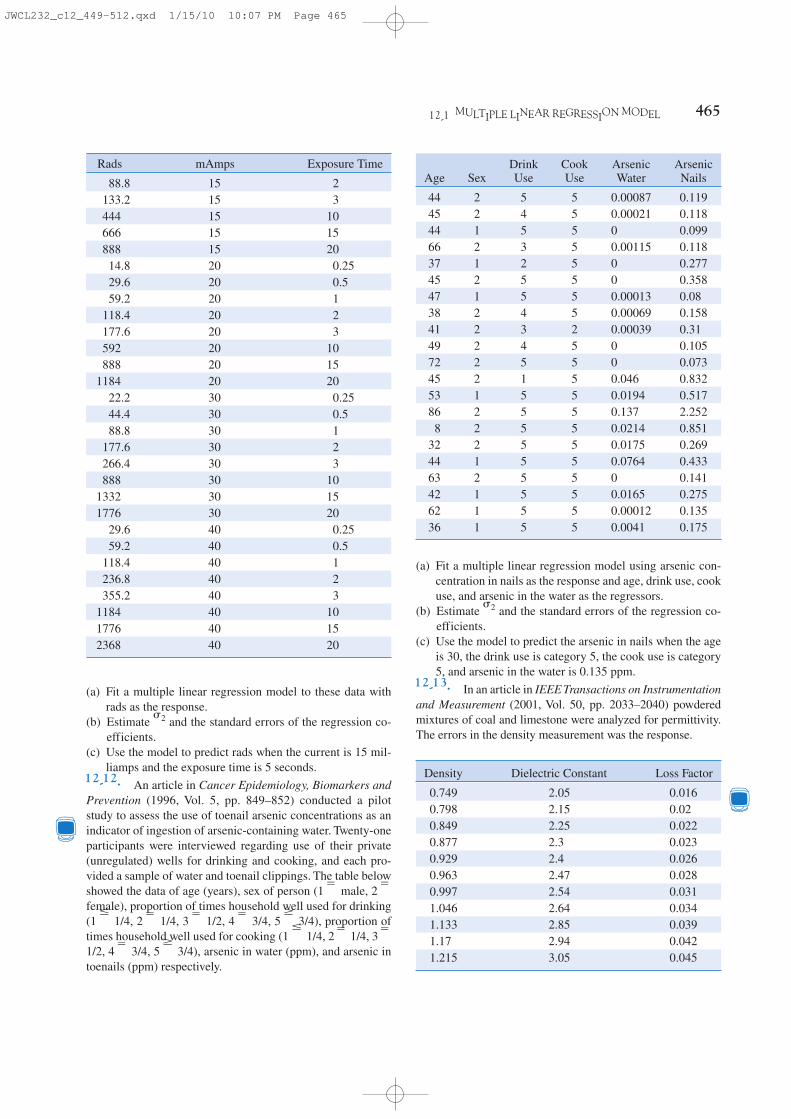
12-1 MULTIPLE LINEAR REGRESSION MODEL 465
Rads mAmps Exposure Time
88.8 15 2133.2 15 3444 15 10666 15 15888 15 2014.8 20 0.2529.6 20 0.559.2 20 1
118.4 20 2177.6 20 3592 20 10888 20 15
1184 20 2022.2 30 0.2544.4 30 0.588.8 30 1
177.6 30 2266.4 30 3888 30 10
1332 30 151776 30 20
29.6 40 0.2559.2 40 0.5
118.4 40 1236.8 40 2355.2 40 3
1184 40 101776 40 152368 40 20
(a) Fit a multiple linear regression model to these data withrads as the response.
(b) Estimate and the standard errors of the regression co-efficients.
(c) Use the model to predict rads when the current is 15 mil-liamps and the exposure time is 5 seconds.
12-12. An article in Cancer Epidemiology, Biomarkers andPrevention (1996, Vol. 5, pp. 849–852) conducted a pilotstudy to assess the use of toenail arsenic concentrations as anindicator of ingestion of arsenic-containing water. Twenty-oneparticipants were interviewed regarding use of their private(unregulated) wells for drinking and cooking, and each pro-vided a sample of water and toenail clippings. The table belowshowed the data of age (years), sex of person (1 ϭ male, 2 ϭfemale), proportion of times household well used for drinking(1 1/4, 2 ϭ 1/4, 3 ϭ 1/2, 4 ϭ 3/4, 5 3/4), proportion oftimes household well used for cooking (1 1/4, 2 ϭ 1/4, 3 ϭ1/2, 4 ϭ 3/4, 5 3/4), arsenic in water (ppm), and arsenic intoenails (ppm) respectively.
Ն
Յ
ՆՅ
2
(a) Fit a multiple linear regression model using arsenic con-centration in nails as the response and age, drink use, cookuse, and arsenic in the water as the regressors.
(b) Estimate and the standard errors of the regression co-efficients.
(c) Use the model to predict the arsenic in nails when the ageis 30, the drink use is category 5, the cook use is category5, and arsenic in the water is 0.135 ppm.
12-13. In an article in IEEE Transactions on Instrumentationand Measurement (2001, Vol. 50, pp. 2033–2040) powderedmixtures of coal and limestone were analyzed for permittivity.The errors in the density measurement was the response.
2
Drink Cook Arsenic ArsenicAge Sex Use Use Water Nails
44 2 5 5 0.00087 0.11945 2 4 5 0.00021 0.11844 1 5 5 0 0.09966 2 3 5 0.00115 0.11837 1 2 5 0 0.27745 2 5 5 0 0.35847 1 5 5 0.00013 0.0838 2 4 5 0.00069 0.15841 2 3 2 0.00039 0.3149 2 4 5 0 0.10572 2 5 5 0 0.07345 2 1 5 0.046 0.83253 1 5 5 0.0194 0.51786 2 5 5 0.137 2.2528 2 5 5 0.0214 0.851
32 2 5 5 0.0175 0.26944 1 5 5 0.0764 0.43363 2 5 5 0 0.14142 1 5 5 0.0165 0.27562 1 5 5 0.00012 0.13536 1 5 5 0.0041 0.175
Density Dielectric Constant Loss Factor
0.749 2.05 0.0160.798 2.15 0.020.849 2.25 0.0220.877 2.3 0.0230.929 2.4 0.0260.963 2.47 0.0280.997 2.54 0.0311.046 2.64 0.0341.133 2.85 0.0391.17 2.94 0.0421.215 3.05 0.045
JWCL232_c12_449-512.qxd 1/15/10 10:07 PM Page 465

466 CHAPTER 12 MULTIPLE LINEAR REGRESSION
Table 12-6
TEMP SOAKTIME SOAKPCT DIFFTIME DIFFPCT PITCH
1650 0.58 1.10 0.25 0.90 0.0131650 0.66 1.10 0.33 0.90 0.0161650 0.66 1.10 0.33 0.90 0.0151650 0.66 1.10 0.33 0.95 0.0161600 0.66 1.15 0.33 1.00 0.0151600 0.66 1.15 0.33 1.00 0.0161650 1.00 1.10 0.50 0.80 0.0141650 1.17 1.10 0.58 0.80 0.0211650 1.17 1.10 0.58 0.80 0.0181650 1.17 1.10 0.58 0.80 0.0191650 1.17 1.10 0.58 0.90 0.0211650 1.17 1.10 0.58 0.90 0.0191650 1.17 1.15 0.58 0.90 0.0211650 1.20 1.15 1.10 0.80 0.0251650 2.00 1.15 1.00 0.80 0.0251650 2.00 1.10 1.10 0.80 0.0261650 2.20 1.10 1.10 0.80 0.0241650 2.20 1.10 1.10 0.80 0.0251650 2.20 1.15 1.10 0.80 0.0241650 2.20 1.10 1.10 0.90 0.0251650 2.20 1.10 1.10 0.90 0.0271650 2.20 1.10 1.50 0.90 0.0261650 3.00 1.15 1.50 0.80 0.0291650 3.00 1.10 1.50 0.70 0.0301650 3.00 1.10 1.50 0.75 0.0281650 3.00 1.15 1.66 0.85 0.0321650 3.33 1.10 1.50 0.80 0.0331700 4.00 1.10 1.50 0.70 0.0391650 4.00 1.10 1.50 0.70 0.0401650 4.00 1.15 1.50 0.85 0.0351700 12.50 1.00 1.50 0.70 0.0561700 18.50 1.00 1.50 0.70 0.068
(a) Fit a multiple linear regression model to these data withthe density as the response.
(b) Estimate and the standard errors of the regressioncoefficients.
(c) Use the model to predict the density when the dielectricconstant is 2.5 and the loss factor is 0.03.
12-14. An article in Biotechnology Progress (2001, Vol.17, pp. 366–368) reported on an experiment to investigate
2
and optimize nisin extraction in aqueous two-phase systems(ATPS). The nisin recovery was the dependent variable ( y).The two regressor variables were concentration (%) of PEG4000 (denoted as and concentration (%) of (de-noted as (a) Fit a multiple linear regression model to these data.(b) Estimate and the standard errors of the regression
coefficients.2
x22. Na2SO4x12
JWCL232_c12_449-512.qxd 1/15/10 10:07 PM Page 466

12-1 MULTIPLE LINEAR REGRESSION MODEL 467
12-17. Table 12-7 presents quarterback ratings for the 2008National Football League season (source: The Sports Network).(a) Fit a multiple regression model to relate the quarterback
rating to the percentage of completions, the percentage ofTDs, and the percentage of interceptions.
(b) Estimate (c) What are the standard errors of the regression coefficients?(d) Use the model to predict the rating when the percentage of
completions is 60%, the percentage of TDs is 4%, and thepercentage of interceptions is 3%.
12-18. Table 12-8 presents statistics for the National HockeyLeague teams from the 2008–2009 season (source: The SportsNetwork). Fit a multiple linear regression model that relatesWins to the variables GF through FG. Because teams play 82games but such a model does nothelp build a better team. Estimate and find the standarderrors of the regression coefficients for your model.12-19. A study was performed on wear of a bearing y and itsrelationship to x1 ϭ oil viscosity and x2 ϭ load. The followingdata were obtained.
2W ϭ 82 Ϫ L Ϫ T Ϫ OTL,
2.
y
13 11 62.873915 11 76.132813 13 87.466715 13 102.323614 12 76.187214 12 77.528714 12 76.782414 12 77.438114 12 78.7417
x2x1
(c) Use the model to predict the nisin recovery whenand
12-15. An article in Optical Engineering [“OperatingCurve Extraction of a Correlator’s Filter” (2004, Vol. 43, pp.2775–2779)] reported on use of an optical correlator to per-form an experiment by varying brightness and contrast. Theresulting modulation is characterized by the useful range ofgray levels. The data are shown below:
Brightness (%): 54 61 65 100 100 100 50 57 54Contrast (%): 56 80 70 50 65 80 25 35 26Useful range (ng): 96 50 50 112 96 80 155 144 255
(a) Fit a multiple linear regression model to these data.(b) Estimate (c) Compute the standard errors of the regression coefficients.(d) Predict the useful range when brightness ϭ 80 and
contrast ϭ 75.12-16. An article in Technometrics (1974, Vol. 16, pp.523–531) considered the following stack-loss data from aplant oxidizing ammonia to nitric acid. Twenty-one daily re-sponses of stack loss y (the amount of ammonia escaping)were measured with air flow temperature , and acid con-centration
Stack loss y ϭ 42, 37, 37, 28, 18, 18, 19, 20, 15, 14, 14, 13,11, 12, 8, 7, 8, 8, 9, 15, 15
x1 ϭ 80, 80, 75, 62, 62, 62, 62, 62, 58, 58, 58, 58, 58, 58, 50,50, 50, 50, 50, 56, 70
x2 ϭ 27, 27, 25, 24, 22, 23, 24, 24, 23, 18, 18, 17, 18, 19, 18,18, 19, 19, 20, 20, 20
x3 ϭ 89, 88, 90, 87, 87, 87, 93, 93, 87, 80, 89, 88, 82, 93, 89,86, 72, 79, 80, 82, 91
(a) Fit a linear regression model relating the results of thestack loss to the three regressor varilables.
(b) Estimate (c) Find the standard error (d) Use the model in part (a) to predict stack loss when
, and x3 ϭ 85.x2 ϭ 26x1 ϭ 60,
se1j2.2.
x3.x2x1,
2.
x2 ϭ 12.5.x1 ϭ 14.5
y x1 x2
293 1.6 851230 15.5 816172 22.0 105891 43.0 1201
113 33.0 1357125 40.0 1115
(a) Fit a multiple linear regression model to these data.(b) Estimate 2 and the standard errors of the regression
coefficients.(c) Use the model to predict wear when x1 ϭ 25 and x2 ϭ 1000.(d) Fit a multiple linear regression model with an interaction
term to these data.(e) Estimate 2 and se( ) for this new model. How did these
quantities change? Does this tell you anything about thevalue of adding the interaction term to the model?
(f) Use the model in (d) to predict when x1 ϭ 25 and x2 ϭ
1000. Compare this prediction with the predicted valuefrom part (c) above.
12-20. Consider the linear regression model
where and (a) Write out the least squares normal equations for this model.(b) Verify that the least squares estimate of the intercept in
this model is (c) Suppose that we use as the response variable in the
model above. What effect will this have on the leastsquares estimate of the intercept?
yi Ϫ y¿0 ϭ g yiրn ϭ y.
x2 ϭg xi2րn.x1 ϭ g xi1րn
Yi ϭ ¿0 ϩ 11xi1 Ϫ x1 2 ϩ 2 1xi2 Ϫ x22 ϩ ⑀i
jˆ
JWCL232_c12_449-512.qxd 1/15/10 10:07 PM Page 467

468 CHAPTER 12 MULTIPLE LINEAR REGRESSION
Table 12-7 Quarterback Ratings for the 2008 National Football League Season
Pct Yds per Pct Pct RatingPlayer Team Att Comp Comp Yds Att TD TD Lng Int Int Pts
Philip Rivers SD 478 312 65.3 4,009 8.39 34 7.1 67 11 2.3 105.5Chad Pennington MIA 476 321 67.4 3,653 7.67 19 4.0 80 7 1.5 97.4Kurt Warner ARI 598 401 67.1 4,583 7.66 30 5.0 79 14 2.3 96.9Drew Brees NO 635 413 65 5,069 7.98 34 5.4 84 17 2.7 96.2Peyton Manning IND 555 371 66.8 4,002 7.21 27 4.9 75 12 2.2 95Aaron Rodgers GB 536 341 63.6 4,038 7.53 28 5.2 71 13 2.4 93.8Matt Schaub HOU 380 251 66.1 3,043 8.01 15 3.9 65 10 2.6 92.7Tony Romo DAL 450 276 61.3 3,448 7.66 26 5.8 75 14 3.1 91.4Jeff Garcia TB 376 244 64.9 2,712 7.21 12 3.2 71 6 1.6 90.2Matt Cassel NE 516 327 63.4 3,693 7.16 21 4.1 76 11 2.1 89.4Matt Ryan ATL 434 265 61.1 3,440 7.93 16 3.7 70 11 2.5 87.7Shaun Hill SF 288 181 62.8 2,046 7.10 13 4.5 48 8 2.8 87.5Seneca Wallace SEA 242 141 58.3 1,532 6.33 11 4.5 90 3 1.2 87Eli Manning NYG 479 289 60.3 3,238 6.76 21 4.4 48 10 2.1 86.4Donovan McNabb PHI 571 345 60.4 3,916 6.86 23 4.0 90 11 1.9 86.4Jay Cutler DEN 616 384 62.3 4,526 7.35 25 4.1 93 18 2.9 86Trent Edwards BUF 374 245 65.5 2,699 7.22 11 2.9 65 10 2.7 85.4Jake Delhomme CAR 414 246 59.4 3,288 7.94 15 3.6 65 12 2.9 84.7Jason Campbell WAS 506 315 62.3 3,245 6.41 13 2.6 67 6 1.2 84.3David Garrard JAC 535 335 62.6 3,620 6.77 15 2.8 41 13 2.4 81.7Brett Favre NYJ 522 343 65.7 3,472 6.65 22 4.2 56 22 4.2 81Joe Flacco BAL 428 257 60 2,971 6.94 14 3.3 70 12 2.8 80.3Kerry Collins TEN 415 242 58.3 2,676 6.45 12 2.9 56 7 1.7 80.2Ben Roethlisberger PIT 469 281 59.9 3,301 7.04 17 3.6 65 15 3.2 80.1Kyle Orton CHI 465 272 58.5 2,972 6.39 18 3.9 65 12 2.6 79.6JaMarcus Russell OAK 368 198 53.8 2,423 6.58 13 3.5 84 8 2.2 77.1Tyler Thigpen KC 420 230 54.8 2,608 6.21 18 4.3 75 12 2.9 76Gus Frerotte MIN 301 178 59.1 2,157 7.17 12 4.0 99 15 5.0 73.7Dan Orlovsky DET 255 143 56.1 1,616 6.34 8 3.1 96 8 3.1 72.6Marc Bulger STL 440 251 57 2,720 6.18 11 2.5 80 13 3.0 71.4Ryan Fitzpatrick CIN 372 221 59.4 1,905 5.12 8 2.2 79 9 2.4 70Derek Anderson CLE 283 142 50.2 1,615 5.71 9 3.2 70 8 2.8 66.5
Att Attempts (number of pass attempts)Comp Completed passesPct Comp Percentage of completed passesYds Yards gained passingYds per Att Yards gained per pass attemptTD Number of touchdown passesPct TD Percentage of attempts that are touchdownsLong Longest pass completionInt Number of interceptionsPct Int Percentage of attempts that are interceptionsRating Pts Rating points
JWCL232_c12_449-512.qxd 1/21/10 9:46 PM Page 468

12-1 MULTIPLE LINEAR REGRESSION MODEL 469
Table 12-8 Team Statistics for the 2008–2009 National Hockey League Season
Team W L OTL PTS GF GA ADV PPGF PCTG PEN BMI AVG SHT PPGA PKPCT SHGF SHGA FG
Anaheim 42 33 7 91 238 235 309 73 23.6 1418 8 17.4 385 78 79.7 6 6 43Atlanta 35 41 6 76 250 279 357 69 19.3 1244 12 15.3 366 88 76 13 9 39Boston 53 19 10 116 270 190 313 74 23.6 1016 12 12.5 306 54 82.4 8 7 47Buffalo 41 32 9 91 242 229 358 75 21 1105 16 13.7 336 61 81.8 7 4 44Carolina 45 30 7 97 236 221 374 70 18.7 786 16 9.8 301 59 80.4 8 7 39Columbus 41 31 10 92 220 223 322 41 12.7 1207 20 15 346 62 82.1 8 9 41Calgary 46 30 6 98 251 246 358 61 17 1281 18 15.8 349 58 83.4 6 13 37Chicago 46 24 12 104 260 209 363 70 19.3 1129 28 14.1 330 64 80.6 10 5 43Colorado 32 45 5 69 190 253 318 50 15.7 1044 18 13 318 64 79.9 4 5 31Dallas 36 35 11 83 224 251 351 54 15.4 1134 10 14 327 70 78.6 2 2 38Detroit 51 21 10 112 289 240 353 90 25.5 810 14 10 327 71 78.3 6 4 46Edmonton 38 35 9 85 228 244 354 60 17 1227 20 15.2 338 76 77.5 3 8 39Florida 41 30 11 93 231 223 308 51 16.6 884 16 11 311 54 82.6 7 6 39Los Angeles 34 37 11 79 202 226 360 69 19.2 1191 16 14.7 362 62 82.9 4 7 39Minnesota 40 33 9 89 214 197 328 66 20.1 869 20 10.8 291 36 87.6 9 6 39Montreal 41 30 11 93 242 240 374 72 19.2 1223 6 15 370 65 82.4 10 10 38New Jersey 51 27 4 106 238 207 307 58 18.9 1038 20 12.9 324 65 79.9 12 3 44Nashville 40 34 8 88 207 228 318 50 15.7 982 12 12.1 338 59 82.5 9 8 41NI Islanders 26 47 9 61 198 274 320 54 16.9 1198 18 14.8 361 73 79.8 12 5 37NY Rangers 43 30 9 95 200 212 346 48 13.9 1175 24 14.6 329 40 87.8 9 13 42Ottawa 36 35 11 83 213 231 339 66 19.5 1084 14 13.4 346 64 81.5 8 5 46Philadelphia 44 27 11 99 260 232 316 71 22.5 1408 26 17.5 393 67 83 16 1 43Phoenix 36 39 7 79 205 249 344 50 14.5 1074 18 13.3 293 68 76.8 5 4 36Pittsburgh 45 28 9 99 258 233 360 62 17.2 1106 8 13.6 347 60 82.7 7 11 46San Jose 53 18 11 117 251 199 360 87 24.2 1037 16 12.8 306 51 83.3 12 10 46St. Louis 41 31 10 92 227 227 351 72 20.5 1226 22 15.2 357 58 83.8 10 8 35Tampa Bay 24 40 18 66 207 269 343 61 17.8 1280 26 15.9 405 89 78 4 8 34Toronto 34 35 13 81 244 286 330 62 18.8 1113 12 13.7 308 78 74.7 6 7 40Vancouver 45 27 10 100 243 213 357 67 18.8 1323 28 16.5 371 69 81.4 7 5 47Washington 50 24 8 108 268 240 337 85 25.2 1021 20 12.7 387 75 80.6 7 9 45
W WinsL Losses during regular timeOTL Overtime lossesPTS Points. Two points for winning a game, one point for
a tie or losing in overtime, zero points for losing inregular time.
GF Goals forGA Goals againstADV Total advantages. Power play opportunities.PPGF Power-play goals for. Goals scored while on power
play.PCTG Power play percentage. Power-play goals divided by
total advantages.
PEN Total penalty minutes including bench minutesBMI Total bench minor minutesAVG Average penalty minutes per gameSHT Total times short-handed. Measures opponent
opportunities.PPGA Power-play goals againstPKPCT Penalty killing percentage. Measures a team’s
ability to prevent goals while its opponent is on apower play. Opponent opportunities minus powerplay goals divided by opponent’s opportunities.
SHGF Short-handed goals forSHGA Short-handed goals againstFG Games scored first
JWCL232_c12_449-512.qxd 1/15/10 10:07 PM Page 469

470 CHAPTER 12 MULTIPLE LINEAR REGRESSION
12-2 HYPOTHESIS TESTS IN MULTIPLE LINEAR REGRESSION
In multiple linear regression problems, certain tests of hypotheses about the model parametersare useful in measuring model adequacy. In this section, we describe several importanthypothesis-testing procedures. As in the simple linear regression case, hypothesis testingrequires that the error terms ⑀i in the regression model are normally and independently dis-tributed with mean zero and variance 2.
12-2.1 Test for Significance of Regression
The test for significance of regression is a test to determine whether a linear relationship existsbetween the response variable y and a subset of the regressor variables x1, x2, p , xk. Theappropriate hypotheses are
(12-18)H1: j Z 0 for at least one j
H0: 1 ϭ 2 ϭ # # # ϭ k ϭ 0
Rejection of implies that at least one of the regressor variablesx1, x2, p , xk contributes significantly to the model.
The test for significance of regression is a generalization of the procedure used in simplelinear regression. The total sum of squares SST is partitioned into a sum of squares due to themodel or to regression and a sum of squares due to error, say,
SST ϭ SSR ϩ SSE
Now if is true, is a chi-square random variable with k de-grees of freedom. Note that the number of degrees of freedom for this chi-square random vari-able is equal to the number of regressor variables in the model. We can also show that theSSE2 is a chi-square random variable with n Ϫ p degrees of freedom, and that SSE and SSR
are independent. The test statistic for isH0: 1 ϭ 2 ϭ p ϭ k ϭ 0
SSRր2H0: 1 ϭ 2 ϭ p ϭ k ϭ 0
H0: 1 ϭ 2 ϭ p ϭ k ϭ 0
(12-19)F0 ϭSSRրk
SSEր 1n Ϫ p2 ϭMSR
MSE
We should reject H0 if the computed value of the test statistic in Equation 12-19, f0, is greater thanf␣,k,nϪp. The procedure is usually summarized in an analysis of variance table such as Table 12-9.
A computational formula for SSR may be found easily. Now since we may rewrite Equation 12-19 as
SSE ϭ y¿y Ϫ
aaniϭ1
yib2
n Ϫ≥ ¿X¿y Ϫ
aaniϭ1
yib2
n¥
1g niϭ1 yi22րn,1g n
iϭ1 yi22րn ϭ y¿y Ϫ
SST ϭgniϭ1 y
2i Ϫ
Hypothesesfor ANOVA Test
Test Statisticfor ANOVA
JWCL232_c12_449-512.qxd 1/15/10 10:07 PM Page 470

12-2 HYPOTHESIS TESTS IN MULTIPLE LINEAR REGRESSION 471
or
SSE ϭ SST Ϫ SSR
Therefore, the regression sum of squares is
(12-21)SSR ϭ ¿X¿y Ϫ
aaniϭ1
yib2
n
Most multiple regression computer programs provide the test for significance of regressionin their output display. The middle portion of Table 12-4 is the Minitab output for this example.Compare Tables 12-4 and 12-10 and note their equivalence apart from rounding. The P-value isrounded to zero in the computer output.
Table 12-9 Analysis of Variance for Testing Significance of Regression in Multiple Regression
Source of Degrees ofVariation Sum of Squares Freedom Mean Square F0
Regression SSR k MSR MSRMSE
Error or residual SSE n Ϫ p MSE
Total SST n Ϫ 1
EXAMPLE 12-3 Wire Bond Strength ANOVAWe will test for significance of regression (with ␣ ϭ 0.05) us-ing the wire bond pull strength data from Example 12-1. Thetotal sum of squares is
The regression or model sum of squares is computed fromEquation 12-20 as follows:
ϭ 5990.7712
SSR ϭ ¿X¿y Ϫ
aaniϭ1
yib2
n ϭ 27,063.3581 Ϫ1725.8222
25
ϭ 6105.9447
SST ϭ y¿y Ϫ
aaniϭ1
yib2
n ϭ 27,178.5316 Ϫ1725.8222
25
and by subtraction
The analysis of variance is shown in Table 12-10. To testwe calculate the statistic
Since f0 Ͼ f0.05,2,22 ϭ 3.44 (or since the P-value is consider-ably smaller than ␣ = 0.05), we reject the null hypothesis andconclude that pull strength is linearly related to either wirelength or die height, or both.
Practical Interpretation: Rejection of H0 does not neces-sarily imply that the relationship found is an appropriatemodel for predicting pull strength as a function of wire lengthand die height. Further tests of model adequacy are requiredbefore we can be comfortable using this model in practice.
f0 ϭMSR
MSEϭ
2995.38565.2352
ϭ 572.17
H0: 1 ϭ 2 ϭ 0,
ϭ y¿y Ϫ ¿X¿y ϭ 115.1716SSE ϭ SST Ϫ SSR
Table 12-10 Test for Significance of Regression for Example 12-3
Source of Degrees of Variation Sum of Squares Freedom Mean Square f0 P-value
Regression 5990.7712 2 2995.3856 572.17 1.08E-19Error or residual 115.1735 22 5.2352Total 6105.9447 24
JWCL232_c12_449-512.qxd 1/15/10 10:07 PM Page 471

472 CHAPTER 12 MULTIPLE LINEAR REGRESSION
R2 and Adjusted R2
We may also use the coefficient of multiple determination R2 as a global statistic to assessthe fit of the model. Computationally,
(12-22)
For the wire bond pull strength data, we find that R2 ϭ SSRSST ϭ 5990.77126105.9447 ϭ
0.9811. Thus the model accounts for about 98% of the variability in the pull strength response(refer to the Minitab output in Table 12-4). The R2 statistic is somewhat problematic as ameasure of the quality of the fit for a multiple regression model because it never decreaseswhen a variable is added to a model.
To illustrate, consider the model fit to the wire bond pull strength data in Example 11-8.This was a simple linear regression model with x1 ϭ wire length as the regressor. The value ofR2 for this model is R2 ϭ 0.9640. Therefore, adding x2 ϭ die height to the model increases R2
by 0.9811 Ϫ 0.9640 ϭ 0.0171, a very small amount. Since R2 can never decrease when aregressor is added, it can be difficult to judge whether the increase is telling us anything usefulabout the new regressor. It is particularly hard to interpret a small increase, such as observedin the pull strength data.
Many regression users prefer to use an adjusted R2 statistic:
R2 ϭSSR
SSTϭ 1 Ϫ
SSE
SST
Because is the error or residual mean square and is a constant, R2adj
will only increase when a variable is added to the model if the new variable reduces the errormean square. Note that for the multiple regression model for the pull strength data R2
adj ϭ
0.979 (see the Minitab output in Table 12-4), whereas in Example 11-8 the adjusted R2 for theone-variable model is R2
adj ϭ 0.962. Therefore, we would conclude that adding x2 ϭ dieheight to the model does result in a meaningful reduction in unexplained variability in theresponse.
The adjusted R2 statistic essentially penalizes the analyst for adding terms to themodel. It is an easy way to guard against overfitting, that is, including regressors that arenot really useful. Consequently, it is very useful in comparing and evaluating competingregression models. We will use R2
adj for this when we discuss variable selection in regres-sion in Section 12-6.3.
12-2.2 Tests on Individual Regression Coefficients and Subsets of Coefficients
We are frequently interested in testing hypotheses on the individual regression coefficients.Such tests would be useful in determining the potential value of each of the regressor variablesin the regression model. For example, the model might be more effective with the inclusion ofadditional variables or perhaps with the deletion of one or more of the regressors presently inthe model.
SSTր 1n Ϫ 12SSEր 1n Ϫ p2(12-23)R2
adj ϭ 1 ϪSSEր 1n Ϫ p2SSTր 1n Ϫ 12
AdjustedR2
JWCL232_c12_449-512.qxd 1/15/10 10:07 PM Page 472

12-2 HYPOTHESIS TESTS IN MULTIPLE LINEAR REGRESSION 473
The hypothesis to test if an individual regression coefficient, say j equals a value j0 is
where Cjj is the diagonal element of corresponding to Notice that the denominator of Equation 12-24 is the standard error of the regression coefficient . The null hypothesis H0: j ϭ j0 is rejected if This is called a partial or marginal test because the regression coefficient depends on all the other regressor variables xi(i � j) that are in themodel. More will be said about this in the following example.
An important special case of the previous hypothesis occurs for j0 ϭ 0. If H0: j ϭ 0 isnot rejected, this indicates that the regressor xj can be deleted from the model. Adding a vari-able to a regression model always causes the sum of squares for regression to increase and theerror sum of squares to decrease (this is why R2 always increases when a variable is added).We must decide whether the increase in the regression sum of squares is large enough to jus-tify using the additional variable in the model. Furthermore, adding an unimportant variableto the model can actually increase the error mean square, indicating that adding such a vari-able has actually made the model a poorer fit to the data (this is why R2
adj is a better measureof global model fit then the ordinary R2).
j
0 t0 0 Ͼ t␣ր2,nϪp.j
j.1X¿X2Ϫ1
(12-24)H1: j � j0
H0: j ϭ j0
(12-25)T0 ϭj Ϫ j0
22Cjj
ϭj Ϫ j0
se1j2
EXAMPLE 12-4 Wire Bond Strength Coefficient TestConsider the wire bond pull strength data, and suppose that wewant to test the hypothesis that the regression coefficient for x2
(die height) is zero. The hypotheses are
The main diagonal element of the matrix correspon-ding to is C22 ϭ 0.0000015, so the t-statistic in Equation12-25 is
t0 ϭ2
22C22
ϭ0.01253
215.23522 10.00000152 ϭ 4.477
2
1X¿X2Ϫ1
H1: 2 � 0
H0: 2 ϭ 0
Note that we have used the estimate of 2 reported to four dec-imal places in Table 12-10. Since t0.025,22 ϭ 2.074, we rejectH0: 2 ϭ 0 and conclude that the variable x2 (die height) con-tributes significantly to the model. We could also have used a P-value to draw conclusions. The P-value for t0 ϭ 4.477 is P ϭ 0.0002, so with ␣ = 0.05 we would reject the null hypothesis.
Practical Interpretation: Note that this test measures themarginal or partial contribution of x2 given that x1 is in themodel. That is, the t-test measures the contribution of addingthe variable x2 ϭ die height to a model that already contains x1
ϭ wire length. Table 12-4 shows the value of the t-test com-puted by Minitab. The Minitab t-test statistic is reported to twodecimal places. Note that the computer produces a t-test foreach regression coefficient in the model. These t-tests indicatethat both regressors contribute to the model.
The test statistic for this hypothesis is
JWCL232_c12_449-512.qxd 1/15/10 10:07 PM Page 473

474 CHAPTER 12 MULTIPLE LINEAR REGRESSION
There is another way to test the contribution of an individual regressor variable to themodel. This approach determines the increase in the regression sum of squares obtained byadding a variable xj (say) to the model, given that other variables xi(i ϶ j) are already includedin the regression equation.
The procedure used to do this is called the general regression significance test, or theextra sum of squares method. This procedure can also be used to investigate the contributionof a subset of the regressor variables to the model. Consider the regression model with kregressor variables
(12-26)
where y is (n ϫ 1), X is (n ϫ p),  is (p ϫ 1), ⑀ is (n ϫ 1), and p ϭ k ϩ 1. We would like to de-termine if the subset of regressor variables x1, x2, . . . , xr (r Ͻ k) as a whole contributes signifi-cantly to the regression model. Let the vector of regression coefficients be partitioned as follows:
(12-27)
where 1 is (r ϫ 1) and 2 is [(p Ϫ r) ϫ 1]. We wish to test the hypotheses
 ϭ c1
2d
y ϭ X ϩ ⑀
Hypothesesfor General
Regression Test (12-28)H1: 1 � 0
H0: 1 ϭ 0
EXAMPLE 12-5 Wire Bond Strength One-Sided Coefficient TestThere is an interest in the effect of die height on strength. Thiscan be evaluated by the magnitude of the coefficient for dieheight. To conclude that the coefficient for die height exceeds0.01 the hypotheses become
For such a test, computer software can complete much of thehard work. We only need to assemble the pieces. From theMinitab output in Table 12-4, and the standard2 ϭ 0.012528
H1: 2 Ͼ 0.01H0: 2 ϭ 0.01
error of Therefore the t-statistic is
with 22 degrees of freedom (error degrees of freedom). FromTable IV in Appendix A, and Therefore, the P-value can be bounded as
One cannot conclude that the coefficient exceeds 0.01at common levels of significance.Ͻ 0.25.
0.1 Ͻ P-valuet0.1, 22 ϭ 1.321.t0.25, 22 ϭ 0.686
t0 ϭ0.012528 Ϫ 0.01
0.002798ϭ 0.9035
2 ϭ 0.002798.
where 0 denotes a vector of zeroes. The model may be written as
(12-29)
where X1 represents the columns of X associated with 1 and X2 represents the columns of Xassociated with 2.
For the full model (including both 1 and 2), we know that Inaddition, the regression sum of squares for all variables including the intercept is
and
MSE ϭy¿y Ϫ X¿y
n Ϫ p
SSR12 ϭ ¿X¿y 1 p ϭ k ϩ 1 degrees of freedom2 ϭ 1X¿X2Ϫ1 X¿y.
y ϭ X ϩ ⑀ ϭ X11 ϩ X22 ϩ ⑀
JWCL232_c12_449-512.qxd 1/15/10 10:07 PM Page 474
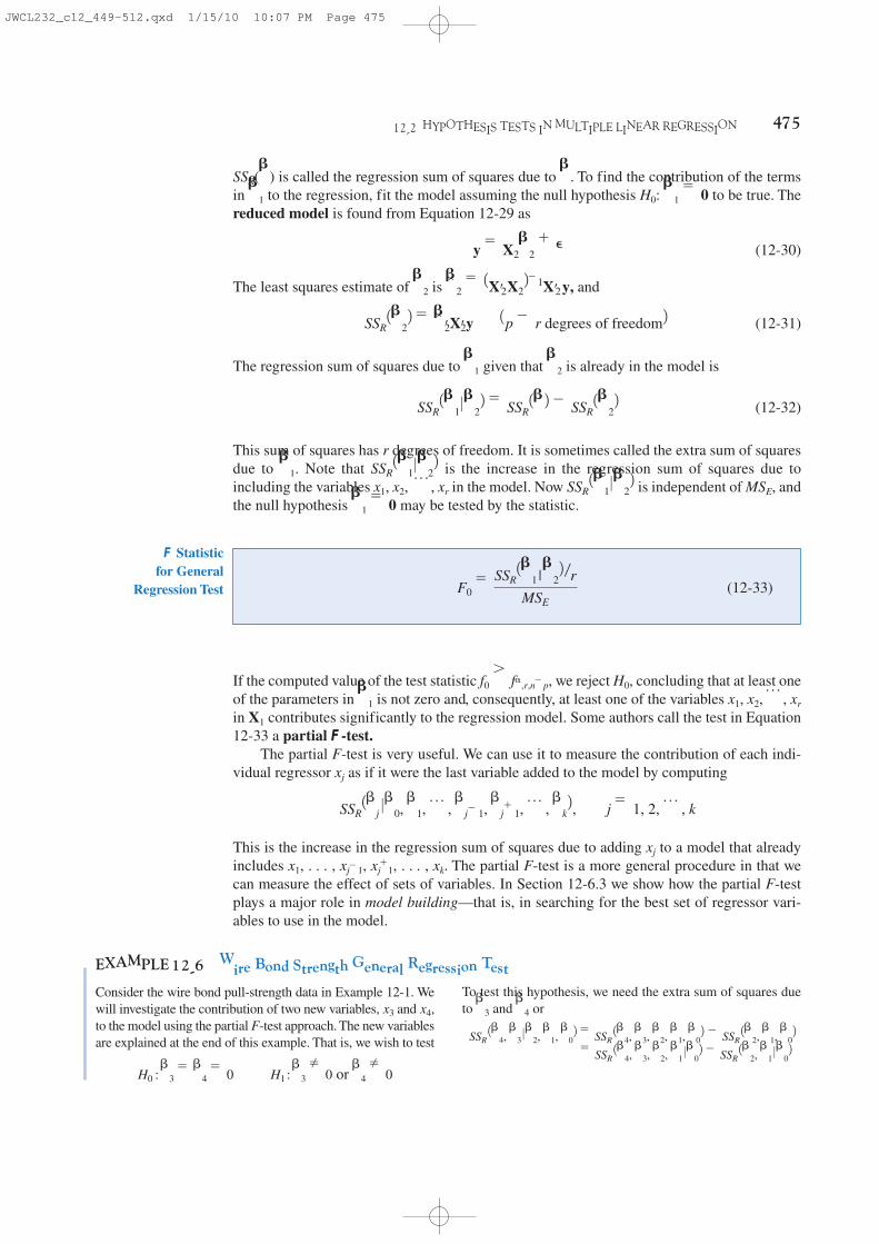
12-2 HYPOTHESIS TESTS IN MULTIPLE LINEAR REGRESSION 475
SSR() is called the regression sum of squares due to . To find the contribution of the termsin 1 to the regression, fit the model assuming the null hypothesis H0: 1 ϭ 0 to be true. Thereduced model is found from Equation 12-29 as
(12-30)
The least squares estimate of 2 is and
(12-31)
The regression sum of squares due to 1 given that 2 is already in the model is
(12-32)
This sum of squares has r degrees of freedom. It is sometimes called the extra sum of squaresdue to 1. Note that is the increase in the regression sum of squares due toincluding the variables x1, x2, p , xr in the model. Now is independent of MSE, andthe null hypothesis 1 ϭ 0 may be tested by the statistic.
SSR11 022SSR11 022SSR11 022 ϭ SSR12 Ϫ SSR122
SSR122 ϭ ¿2X¿2y 1p Ϫ r degrees of freedom22 ϭ 1X¿2X22Ϫ1X¿2y,
y ϭ X22 ϩ ⑀
(12-33)F0 ϭSSR11 |22րr
MSE
F Statistic for General
Regression Test
If the computed value of the test statistic f0 Ͼ f␣,r,nϪp, we reject H0, concluding that at least oneof the parameters in 1 is not zero and, consequently, at least one of the variables x1, x2, p , xr
in X1 contributes significantly to the regression model. Some authors call the test in Equation12-33 a partial F -test.
The partial F-test is very useful. We can use it to measure the contribution of each indi-vidual regressor xj as if it were the last variable added to the model by computing
This is the increase in the regression sum of squares due to adding xj to a model that alreadyincludes x1, . . . , xjϪ1, xjϩ1, . . . , xk. The partial F-test is a more general procedure in that wecan measure the effect of sets of variables. In Section 12-6.3 we show how the partial F-testplays a major role in model building—that is, in searching for the best set of regressor vari-ables to use in the model.
SSR1j 00, 1, p , jϪ1, jϩ1, p , k2, j ϭ 1, 2, p , k
EXAMPLE 12-6 Wire Bond Strength General Regression TestConsider the wire bond pull-strength data in Example 12-1. Wewill investigate the contribution of two new variables, and to the model using the partial F-test approach. The new variablesare explained at the end of this example. That is, we wish to test
or 4 � 0H1 : 3 � 0H0 : 3 ϭ 4 ϭ 0
x4,x3
To test this hypothesis, we need the extra sum of squares dueto and or
ϭ SSR 14, 3, 2, 1 002 Ϫ SSR 12, 1 002Ϫ SSR 12, 1, 02SSR 14, 3 02, 1, 02 ϭ SSR 14, 3, 2, 1, 0243
JWCL232_c12_449-512.qxd 1/15/10 10:07 PM Page 475

476 CHAPTER 12 MULTIPLE LINEAR REGRESSION
If a partial F-test is applied to a single variable, it is equivalent to a t-test. To see this, con-sider the Minitab regression output for the wire bond pull strength in Table 12-4. Just belowthe analysis of variance summary in this table, the quantity labeled ” ‘SeqSS”’ shows the sum
In Example 12-3 we calculated
(twodegrees of freedom)
Also, Table 12-4 shows the Minitab output for the model withonly and as predictors. In the analysis of variance table,we can see that and this agrees with our calcu-lation. In practice, the computer output would be used to ob-tain this sum of squares.
If we fit the model we can use the same matrix formula. Alternatively, we can
look at from computer output for this model. The analysisof variance table for this model is shown in Table 12-11 and wesee that
6024.0 (four degrees of freedom)
Therefore,
(two degrees of freedom)
SSR 14, 3 02, 1, 02 ϭ 6024.0 Ϫ 5990.8 ϭ 33.2
SSR 14, 3, 2, 1 002 ϭ
SSR
4x4,Y ϭ 0 ϩ 1x1 ϩ 2x2 ϩ 3x3 ϩ
SSR ϭ 5990.8x2x1
SSR 12, 1 0022 ϭ ¿Xy Ϫ
aaniϭ1
yib2
n ϭ 5990.7712
This is the increase in the regression sum of squares due toadding and to a model already containing and Totest calculate the test statistic
Note that from the full model using and is used in the denominator of the test statistic. Because
we reject and conclude that at least oneof the new variables contributes significantly to the model.Further analysis and tests will be needed to refine the modeland determine if one or both of and are important.
The mystery of the new variables can now be explained.These are quadratic powers of the original predictors wirelength and wire height. That is, and A test forquadratic terms is a common use of partial F-tests. With thisinformation and the original data for and you can usecomputer software to reproduce these calculations. Multipleregression allows models to be extended in such a simple man-ner that the real meaning of and did not even enter intothe test procedure. Polynomial models such as this are dis-cussed further in Section 12-6.
x4x3
x2,x1
x4 ϭ x22.x3 ϭ x2
1
x4x3
H0f0.05, 2, 20 ϭ 3.49,
x4x3x2,x1,MSE
f0 ϭSSR 14, 3 02, 1, 02ր2
MSEϭ
33.2ր24.1
ϭ 4.05
H0,x2.x1x4x3
Table 12-11 Regression Analysis: y versus x1, x2, x3, x4
The regression equation is y ϭ 5.00 ϩ 1.90 x1 + 0.0151 x2 + 0.0460 x3 Ϫ 0.000008 x4
Predictor Coef SE Coef T PConstant 4.996 1.655 3.02 0.007x1 1.9049 0.3126 6.09 0.000x2 0.01513 0.01051 1.44 0.165x3 0.04595 0.01666 2.76 0.012x4 0.00001641 0.646
S ϭ 2.02474 RϪSq ϭ 98.7% RϪSq (adj) ϭ 98.4%
Analysis of Variance
Source DF SS MS F PRegression 4 6024.0 1506.0 367.35 0.000Residual Error 20 82.0 4.1Total 24 6105.9
Source DF Seq SSx1 1 5885.9x2 1 104.9x3 1 32.3x4 1 0.9
Ϫ0.47Ϫ0.00000766
JWCL232_c12_449-512.qxd 1/21/10 9:23 PM Page 476

12-2 HYPOTHESIS TESTS IN MULTIPLE LINEAR REGRESSION 477
of squares obtained by fitting alone (5885.9) and the sum of squares obtained by fitting after (104.9). In out notation, these are referred to as and respec-tively. Therefore, to test , the partial F-test is
where is the mean square for residual in the computer output in Table 12.4. This statisticshould be compared to an F-distribution with 1 and 22 degrees of freedom in the numeratorand denominator, respectively. From Table 12-4, the t-test for the same hypothesis is Note that except for round-off error. Furthermore, the square of at-random variable with degrees of freedom is an F-random variable with one and degrees offreedom. Consequently, the t-test provides an equivalent method to test a single variable forcontribution to a model. Because the t-test is typically provided by computer output, it is thepreferred method to test a single variable.
t20 ϭ 4.482 ϭ 20.07 ϭ f0,
t0 ϭ 4.48.
MSE
f0 ϭSSR 12 01, 02ր1
MSEϭ
104.925.24
ϭ 20.2
H1 : 2 � 0H0 : 2 ϭ 0SSR 12, 1 002,SSR 11 002x1
x2x1
EXERCISES FOR SECTION 12-2
12-21. Consider the computer output below.
The regression equation isY ϭ 254 ϩ 2.77 x1 Ϫ 3.58 x2
Predictor Coef SE Coef T PConstant 253.810 4.781 ? ?x1 2.7738 0.1846 15.02 ?x2 Ϫ3.5753 0.1526 ? ?
S ϭ 5.05756 R-Sq ϭ ? R-Sq (adj) ϭ 98.4%
Analysis of Variance
Source DF SS MS F PRegression 2 22784 11392 ? ?Residual Error ? ? ?Total 14 23091
(a) Fill in the missing quantities. You may use bounds for theP-values.
(b) What conclusions can you draw about the significance ofregression?
(c) What conclusions can you draw about the contributions ofthe individual regressors to the model?
12-22. You have fit a regression model with two regressorsto a data set that has 20 observations. The total sum of squaresis 1000 and the model sum of squares is 750.(a) What is the value of R2 for this model?(b) What is the adjusted R2 for this model?(c) What is the value of the F-statistic for testing the signifi-
cance of regression? What conclusions would you drawabout this model if ␣ ϭ 0.05? What if ␣ ϭ 0.01?
(d) Suppose that you add a third regressor to the model and asa result the model sum of squares is now 785. Does it seemto you that adding this factor has improved the model?
12-23. Consider the regression model fit to the soil shearstrength data in Exercise 12-1.
(a) Test for significance of regression using ␣ ϭ 0.05. Whatis the P-value for this test?
(b) Construct the t-test on each regression coefficient. Whatare your conclusions, using ␣ ϭ 0.05? Calculate P-values.
12-24. Consider the absorption index data in Exercise 12-2.The total sum of squares for y is SST ϭ 742.00.(a) Test for significance of regression using ␣ ϭ 0.01. What
is the P-value for this test?(b) Test the hypothesis H0: 1 ϭ 0 versus H1: 1 � 0 using
␣ ϭ 0.01. What is the P-value for this test?(c) What conclusion can you draw about the usefulness of x1
as a regressor in this model?
12-25. A regression model Y ϭ 0 ϩ 1x1 ϩ 2x2 ϩ 3x3 ϩ
⑀ has been fit to a sample of n ϭ 25 observations. The calcu-lated t-ratios are as follows: for 1, t0 ϭ
4.82, for 2, t0 ϭ 8.21 and for 3, t0 ϭ 0.98. (a) Find P-values for each of the t-statistics.(b) Using ␣ ϭ 0.05, what conclusions can you draw about
the regressor x3? Does it seem likely that this regressorcontributes significantly to the model?
12-26. Consider the electric power consumption data inExercise 12-6.(a) Test for significance of regression using ␣ ϭ 0.05. What
is the P-value for this test?(b) Use the t-test to assess the contribution of each regressor
to the model. Using ␣ ϭ 0.05, what conclusions can youdraw?
12-27. Consider the gasoline mileage data in Exercise 12-7.(a) Test for significance of regression using ␣ ϭ 0.05. What
conclusions can you draw?(b) Find the t-test statistic for each regressor. Using ␣ ϭ 0.05,
what conclusions can you draw? Does each regressor con-tribute to the model?
j րse 1j2, j ϭ 1, 2, 3
JWCL232_c12_449-512.qxd 1/16/10 10:52 AM Page 477

478 CHAPTER 12 MULTIPLE LINEAR REGRESSION
12-28. Consider the wire bond pull strength data inExercise 12-8.(a) Test for significance of regression using ␣ ϭ 0.05. Find
the P-value for this test. What conclusions can youdraw?
(b) Calculate the t-test statistic for each regression coeffi-cient. Using ␣ ϭ 0.05, what conclusions can you draw?Do all variables contribute to the model?
12-29. Reconsider the semiconductor data in Exercise 12-9.(a) Test for significance of regression using ␣ ϭ 0.05. What
conclusions can you draw?(b) Calculate the t-test statistic and P-value for each regres-
sion coefficient. Using ␣ ϭ 0.05, what conclusions canyou draw?
12-30. Consider the regression model fit to the arsenic datain Exercise 12-12. Use arsenic in nails as the response and age,drink use, and cook use as the regressors.(a) Test for significance of regression using What
is the P-value for this test?(b) Construct a t-test on each regression coefficient. What
conclusions can you draw about the variables in thismodel? Use
12-31. Consider the regression model fit to the X-ray in-spection data in Exercise 12-11. Use rads as the response.(a) Test for significance of regression using What
is the P-value for this test?(b) Construct a t-test on each regression coefficient. What
conclusions can you draw about the variables in thismodel? Use
12-32. Consider the regression model fit to the nisin extrac-tion data in Exercise 12-14. Use nisin extraction as the response.(a) Test for significance of regression using What
is the P-value for this test?(b) Construct a t-test on each regression coefficient. What
conclusions can you draw about the variables in thismodel? Use
(c) Comment on the effect of a small sample size to the testsin the previous parts.
12-33. Consider the regression model fit to the grey rangemodulation data in Exercise 12-15. Use the useful range as theresponse.(a) Test for significance of regression using What
is the P-value for this test?(b) Construct a t-test on each regression coefficient. What
conclusions can you draw about the variables in thismodel? Use
12-34. Consider the regression model fit to the stack lossdata in Exercise 12-16. Use stack loss as the response.(a) Test for significance of regression using What
is the P-value for this test?(b) Construct a t-test on each regression coefficient. What
conclusions can you draw about the variables in thismodel? Use ␣ ϭ 0.05.
␣ ϭ 0.05.
␣ ϭ 0.05.
␣ ϭ 0.05.
␣ ϭ 0.05.
␣ ϭ 0.05.
␣ ϭ 0.05.
␣ ϭ 0.05.
␣ ϭ 0.05.
␣ ϭ 0.05.
12-35. Consider the NFL data in Exercise 12-17.(a) Test for significance of regression using ␣ ϭ 0.05. What
is the P-value for this test?(b) Conduct the t-test for each regression coefficient. Using
␣ ϭ 0.05, what conclusions can you draw about the vari-ables in this model?
(c) Find the amount by which the regressor x2 (TD percent-age) increases the regression sum of squares, and conductan F-test for H0: 2 ϭ 0 versus H1: 2 ϶ 0 using␣ ϭ 0.05. What is the P-value for this test? What conclu-sions can you draw?
12-36. Exercise 12-10 presents data on heat treating gears.(a) Test the regression model for significance of regression.
Using ␣ ϭ 0.05, find the P-value for the test and drawconclusions.
(b) Evaluate the contribution of each regressor to the modelusing the t-test with ␣ ϭ 0.05.
(c) Fit a new model to the response PITCH using newregressors x1 ϭ SOAKTIME ϫ SOAKPCT and x2 ϭ
DIFFTIME ϫ DIFFPCT.(d) Test the model in part (c) for significance of regression
using ␣ ϭ 0.05. Also calculate the t-test for each regres-sor and draw conclusions.
(e) Estimate 2 for the model from part (c) and compare thisto the estimate of 2 for the model in part (a). Whichestimate is smaller? Does this offer any insight regardingwhich model might be preferable?
12-37. Consider the bearing wear data in Exercise 12-19.(a) For the model with no interaction, test for significance of
regression using ␣ ϭ 0.05. What is the P-value for thistest? What are your conclusions?
(b) For the model with no interaction, compute the t-statisticsfor each regression coefficient. Using ␣ ϭ 0.05, what con-clusions can you draw?
(c) For the model with no interaction, use the extra sum ofsquares method to investigate the usefulness of adding x2 ϭ load to a model that already contains x1 ϭ oil vis-cosity. Use ␣ ϭ 0.05.
(d) Refit the model with an interaction term. Test for signifi-cance of regression using ␣ ϭ 0.05.
(e) Use the extra sum of squares method to determine whetherthe interaction term contributes significantly to the model.Use ␣ ϭ 0.05.
(f) Estimate 2 for the interaction model. Compare this to theestimate of 2 from the model in part (a).
12-38. Data on National Hockey League team performancewas presented in Exercise 12-18.(a) Test the model from this exercise for significance of
regression using ␣ ϭ 0.05. What conclusions can you draw?(b) Use the t-test to evaluate the contribution of each
regressor to the model. Does it seem that all regressors arenecessary? Use ␣ ϭ 0.05.
(c) Fit a regression model relating the number of games won tothe number of goals for and the number of power play goals
JWCL232_c12_449-512.qxd 1/15/10 10:07 PM Page 478

12-3 CONFIDENCE INTERVALS IN MULTIPLE LINEAR REGRESSION 479
for. Does this seem to be a logical choice of regressors, con-sidering your answer to part (b)? Test this new model forsignificance of regression and evaluate the contribution ofeach regressor to the model using the t-test. Use ␣ ϭ 0.05.
12-39. Data from a hospital patient satisfaction survey werepresented in Exercise 12-5.(a) Test the model from this exercise for significance of regression.
What conclusions can you draw if ␣ ϭ 0.05? What if ␣ ϭ 0.01?(b) Test the contribution of the individual regressors using the
t-test. Does it seem that all regressors used in the model arereally necessary?
12-40. Data from a hospital patient satisfaction survey werepresented in Exercise 12-5.
(a) Fit a regression model using only the patient age and severityregressors. Test the model from this exercise for significanceof regression. What conclusions can you draw if ␣ ϭ 0.05?What if ␣ ϭ 0.01?
(b) Test the contribution of the individual regressors using thet-test. Does it seem that all regressors used in the model arereally necessary?
(c) Find an estimate of the error variance 2. Compare this esti-mate of 2 with the estimate obtained from the model con-taining the third regressor, anxiety. Which estimate issmaller? Does this tell you anything about which modelmight be preferred?
12-3 CONFIDENCE INTERVALS IN MULTIPLE LINEAR REGRESSION
12-3.1 Confidence Intervals on Individual Regression Coefficients
In multiple regression models, it is often useful to construct confidence interval estimates forthe regression coefficients The development of a procedure for obtaining these confi-dence intervals requires that the errors are normally and independently distributed withmean zero and variance 2. This is the same assumption required in hypothesis testing.Therefore, the observations {Yi} are normally and independently distributed with mean 0 ϩ
gkjϭ1 jxij and variance 2. Since the least squares estimator is a linear combination of the
observations, it follows that is normally distributed with mean vector  and covariance matrix . Then each of the statistics
(12-34)
has a t distribution with n Ϫ p degrees of freedom, where Cjj is the jjth element of the matrix, and is the estimate of the error variance, obtained from Equation 12-16. This leads to the following 100(1 Ϫ ␣)% confidence interval for the regression coefficient j, j ϭ 0, 1, p , k.
21X¿X2Ϫ1
T ϭj Ϫ j
22Cjj
j ϭ 0, 1, p , k
21X¿X2Ϫ1

5⑀i65j 6.
A 100(1 Ϫ ␣) % confidence interval on the regression coefficient j, j ϭ 0, 1, p ,k in the multiple linear regression model is given by
(12-35)j Ϫ t␣ր2,nϪp22Cjj Յ j Յ j ϩ t␣ր2,nϪp22Cjj
Confidence Interval on a
Regression Coefficient
Because is the standard error of the regression coefficient , we would also write the CI formula as j Ϫ t␣ր2,nϪp se1j2 Յ j Յ j ϩ t␣ր2,nϪp se1j2. j22Cjj
JWCL232_c12_449-512.qxd 1/15/10 10:07 PM Page 479

480 CHAPTER 12 MULTIPLE LINEAR REGRESSION
For the multiple linear regression model, a 100(1 Ϫ ␣)% confidence interval on themean response at the point x01, x02, . . . , x0k is
(12-39)Յ Y 0x0Յ Y 0x0
ϩ t␣ր2,nϪp22˛x¿0 1�¿�2Ϫ1 x0
Y 0x0Ϫ t␣ր2,nϪp22
˛x¿0 1X¿X2Ϫ1 x0
Confidence Interval on the
Mean Response
EXAMPLE 12-7 Wire Bond Strength Confidence IntervalWe will construct a 95% confidence interval on the parameter 1
in the wire bond pull strength problem. The point estimate of 1
is and the diagonal element of corre-sponding to 1 is C11 ϭ 0.001671. The estimate of 2 is
and t0.025,22 ϭ 2.074. Therefore, the 95% CI on 1
is computed from Equation 12-35 as
which reduces to
2.55029 Յ 1 Յ 2.93825
ϩ 12.0742215.23522 1.00167122.74427 Ϫ 12.0742215.23522 1.0016712 Յ 1 Յ 2.74427
2 ϭ 5.2352,
1X¿X2Ϫ11 ϭ 2.74427
Also, computer software such as Minitab can be used to helpcalculate this confidence interval. From the regression outputin Table 10-4, and the standard error of
This standard error is the multiplier of the t-table constant in the confidence interval. That is, 0.0935 ϭ
Consequently, all the numbers areavailable from the computer output to construct the intervaland this is the typical method used in practice.
115.23522 10.0016712.1 ϭ 0.0935.1 ϭ 2.74427
12-3.2 Confidence Interval on the Mean Response
We may also obtain a confidence interval on the mean response at a particular point, say,x01, x02, p , x0k. To estimate the mean response at this point, define the vector
The mean response at this point is which is estimated by
(12-36)
This estimator is unbiased, since and the variance of is
(12-37)
A 100(1 Ϫ ␣) % CI on can be constructed from the statistic
(12-38)Y 0 x0
Ϫ Y 0 x0
22˛x¿0 1X¿X2Ϫ1 x0
Y 0 x0
V1Y 0 x02 ϭ 2x¿01X¿X2Ϫ1x0
Y 0 x0E1x¿02 ϭ x¿0 ϭ E1Y 0 x02 ϭ Y 0 x0
Y 0 x0ϭ x¿0
E1Y 0 x02 ϭ Y 0 x0ϭ x¿0,
x0 ϭ
1x01
x02
o
x0k
M m
JWCL232_c12_449-512.qxd 1/15/10 10:08 PM Page 480

12-4 PREDICTION OF NEW OBSERVATIONS 481
EXAMPLE 12-8 Wire Bond Strength Confidence Interval on the Mean ResponseThe engineer in Example 12-1 would like to construct a 95%CI on the mean pull strength for a wire bond with wire lengthx1 ϭ 8 and die height x2 ϭ 275. Therefore,
The estimated mean response at this point is found fromEquation 12-36 as
The variance of is estimated by
ϭ 5.2352 10.04442 ϭ 0.23244
ϫ £ .214653 Ϫ.007491 Ϫ.000340Ϫ.007491 .001671 Ϫ.000019Ϫ.000340 Ϫ.000019 .0000015
§ £ 18
275§
2x0¿ 1�¿�2Ϫ1x0 ϭ 5.2352 31 8 275 4Y 0x0
Y |x0ϭ x0¿  ϭ 31 8 275 4 £ 2.26379
2.744270.01253
§ ϭ 27.66
x0 ϭ £ 18
275§
Therefore, a 95% CI on the mean pull strength at this point isfound from Equation 12-39 as
which reduces to
Some computer software packages will provide estimates ofthe mean for a point of interest x0 and the associated CI. Table12-4 shows the Minitab output for Example 12-8. Both the es-timate of the mean and the 95% CI are provided.
26.66 Յ Y |x0Յ 28.66
ϩ 2.074 10.23244
27.66 Ϫ 2.07410.23244 Յ Y 0x0Յ 27.66
Equation 12-39 is a CI about the regression plane (or hyperplane). It is the multiple regressiongeneralization of Equation 11-32.
12-4 PREDICTION OF NEW OBSERVATIONS
A regression model can be used to predict new or future observations on the responsevariable Y corresponding to particular values of the independent variables, say, x01, x02, p , x0k.If , a point estimate of the future observation Y0 at the point x01, x02, p , x0k is
(12-40)y0 ϭ x¿0 ˛
x¿0 ϭ 31, x01, x02, p , x0k 4
A 100(1 Ϫ ␣)% prediction interval for this future observation is
(12-41)Յ Y0 Յ y0 ϩ t␣ր2,nϪp22˛11 ϩ x¿0 1�¿�2Ϫ1 x02y0 Ϫ t␣ր2,nϪp22
˛11 ϩ x¿0 1�¿�2Ϫ1 x02Prediction
Interval
This prediction interval is a generalization of the prediction interval given in Equation 11-33for a future observation in simple linear regression. If you compare the prediction intervalEquation 12-41 with the expression for the confidence interval on the mean, Equation 12-39,
JWCL232_c12_449-512.qxd 1/15/10 10:08 PM Page 481

482 CHAPTER 12 MULTIPLE LINEAR REGRESSION
Figure 12-5 An example of extrapolation in multiple regression.
x01
x01
x2
Joint region
of original area
Original range for x1
x1
Ori
gin
al ra
nge f
or
x2
you will observe that the prediction interval is always wider than the confidence interval. Theconfidence interval expresses the error in estimating the mean of a distribution, while the pre-diction interval expresses the error in predicting a future observation from the distribution atthe point x0. This must include the error in estimating the mean at that point, as well as the in-herent variability in the random variable Y at the same value x ϭ x0.
Also, one might want to predict the mean of several values of Y, say m, all at the samevalue x = x0. Because the variance of a sample mean is 2/m, Equation 12-41 is modified asfollows. Replace the constant 1 under the square root with 1/m to reflect the lower variabilityin the mean of m observations. This results in a narrower interval.
In predicting new observations and in estimating the mean response at a given pointx01, x02, . . . , x0k, we must be careful about extrapolating beyond the region containing theoriginal observations. It is very possible that a model that fits well in the region of the origi-nal data will no longer fit well outside of that region. In multiple regression it is often easyto inadvertently extrapolate, since the levels of the variables (xi1, xi2, . . . , xik), i ϭ 1, 2, . . . , n,jointly define the region containing the data. As an example, consider Fig. 12-5, which illus-trates the region containing the observations for a two-variable regression model. Note thatthe point (x01, x02) lies within the ranges of both regressor variables x1 and x2, but it is outside theregion that is actually spanned by the original observations. This is sometimes called a hiddenextrapolation. Either predicting the value of a new observation or estimating the mean re-sponse at this point is an extrapolation of the original regression model.
EXAMPLE 12-9 Wire Bond Strength Confidence IntervalSuppose that the engineer in Example 12-1 wishes to con-struct a 95% prediction interval on the wire bond pull strengthwhen the wire length is x1 ϭ 8 and the die height is x2 ϭ 275.Note that ϭ [1 8 275], and the point estimate of thepull strength is Also, in Example 12-8we calculated Therefore, fromEquation 12-41 we have
ϩ 2.074 25.235211 ϩ 0.0444227.66 Ϫ 2.074˛25.235211 ϩ 0.04442 Յ Y0 Յ 27.66
x¿0 1�¿�2Ϫ1x0 ϭ 0.04444.y0 ϭ x¿0  ϭ 27.66.
x¿0
and the 95% prediction interval is
Notice that the prediction interval is wider than the confidenceinterval on the mean response at the same point, calculated inExample 12-8. The Minitab output in Table 12-4 also displaysthis prediction interval.
22.81 Յ Y0 Յ 32.51
JWCL232_c12_449-512.qxd 1/15/10 10:08 PM Page 482
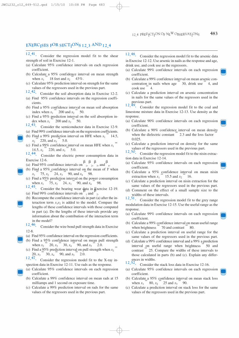
EXERCISES FOR SECTIONS 12-3 AND 12-4
12-4 PREDICTION OF NEW OBSERVATIONS 483
12-41. Consider the regression model fit to the shearstrength of soil in Exercise 12-1.(a) Calculate 95% confidence intervals on each regression
coefficient.(b) Calculate a 95% confidence interval on mean strength
when feet and (c) Calculate 95% prediction interval on strength for the same
values of the regressors used in the previous part.
12-42. Consider the soil absorption data in Exercise 12-2.(a) Find 95% confidence intervals on the regression coeffi-
cients.(b) Find a 95% confidence interval on mean soil absorption
index when x1 ϭ 200 and x2 ϭ 50.(c) Find a 95% prediction interval on the soil absorption in-
dex when x1 ϭ 200 and x2 ϭ 50.
12-43. Consider the semiconductor data in Exercise 12-9.(a) Find 99% confidence intervals on the regression coefficients.(b) Find a 99% prediction interval on HFE when x1 ϭ 14.5,
x2 ϭ 220, and x3 ϭ 5.0.(c) Find a 99% confidence interval on mean HFE when x1 ϭ
14.5, x2 ϭ 220, and x3 ϭ 5.0.
12-44. Consider the electric power consumption data inExercise 12-6.(a) Find 95% confidence intervals on 1, 2, 3, and 4.(b) Find a 95% confidence interval on the mean of Y when
x1 ϭ 75, x2 ϭ 24, x3 ϭ 90, and x4 ϭ 98.(c) Find a 95% prediction interval on the power consumption
when x1 ϭ 75, x2 ϭ 24, x3 ϭ 90, and x4 ϭ 98.
12-45. Consider the bearing wear data in Exercise 12-19.(a) Find 99% confidence intervals on 1 and 2.(b) Recompute the confidence intervals in part (a) after the in-
teraction term x1x2 is added to the model. Compare thelengths of these confidence intervals with those computedin part (a). Do the lengths of these intervals provide anyinformation about the contribution of the interaction termin the model?
12-46. Consider the wire bond pull strength data in Exercise12-8.(a) Find 95% confidence interval on the regression coefficients.(b) Find a 95% confidence interval on mean pull strength
when x2 ϭ 20, x3 ϭ 30, x4 ϭ 90, and x5 ϭ 2.0.(c) Find a 95% prediction interval on pull strength when x2 ϭ
20, x3 ϭ 30, x4 ϭ 90, and x5 ϭ 2.0.
12-47. Consider the regression model fit to the X-ray in-spection data in Exercise 12-11. Use rads as the response.(a) Calculate 95% confidence intervals on each regression
coefficient.(b) Calculate a 99% confidence interval on mean rads at 15
milliamps and 1 second on exposure time.(c) Calculate a 99% prediction interval on rads for the same
values of the regressors used in the previous part.
x2 ϭ 43%.x1 ϭ 18
12-48. Consider the regression model fit to the arsenic datain Exercise 12-12. Use arsenic in nails as the response and age,drink use, and cook use as the regressors.(a) Calculate 99% confidence intervals on each regression
coefficient.(b) Calculate a 99% confidence interval on mean arsenic con-
centration in nails when drink andcook
(c) Calculate a prediction interval on arsenic concentrationin nails for the same values of the regressors used in theprevious part.
12-49. Consider the regression model fit to the coal andlimestone mixture data in Exercise 12-13. Use density as theresponse.(a) Calculate 90% confidence intervals on each regression
coefficient.(b) Calculate a 90% confidence interval on mean density
when the dielectric and the loss factor ϭ
(c) Calculate a prediction interval on density for the samevalues of the regressors used in the previous part.
12-50. Consider the regression model fit to the nisin extrac-tion data in Exercise 12-14.(a) Calculate 95% confidence intervals on each regression
coefficient.(b) Calculate a 95% confidence interval on mean nisin
extraction when and (c) Calculate a prediction interval on nisin extraction for the
same values of the regressors used in the previous part.(d) Comment on the effect of a small sample size to the
widths of these intervals.12-51. Consider the regression model fit to the grey rangemodulation data in Exercise 12-15. Use the useful range as theresponse.(a) Calculate 99% confidence intervals on each regression
coefficient.(b) Calculate a 99% confidence interval on mean useful range
when and (c) Calculate a prediction interval on useful range for the
same values of the regressors used in the previous part.(d) Calculate a 99% confidence interval and a 99% a prediction
interval on useful range when andCompare the widths of these intervals to
those calculated in parts (b) and (c). Explain any differ-ences in widths.
12-52. Consider the stack loss data in Exercise 12-16.(a) Calculate 95% confidence intervals on each regression
coefficient.(b) Calculate a 95% confidence interval on mean stack loss
when and (c) Calculate a prediction interval on stack loss for the same
values of the regressors used in the previous part.
x3 ϭ 90.x2 ϭ 25x1 ϭ 80,
contrast ϭ 25.brightness ϭ 50
contrast ϭ 80.brightness ϭ 70
x2 ϭ 16.x1 ϭ 15.5
0.025.constant ϭ 2.3
use ϭ 4.use ϭ 4,age ϭ 30,
JWCL232_c12_449-512.qxd 1/15/10 10:08 PM Page 483

(12-42)di ϭei
2MSE
ϭei
22
StandardizedResidual
(d) Calculate a 95% confidence interval and a 95% predictioninterval on stack loss when , and Compare the widths of these intervals to those calculatedin parts (b) and (c). Explain any differences in widths.
12-53. Consider the NFL data in Exercise 12-17.(a) Find 95% confidence intervals on the regression coefficients.(b) What is the estimated standard error of when the
percentage of completions is 60%, the percentage of TDsis 4%, and the percentage of interceptions is 3%.
(c) Find a 95% confidence interval on the mean rating whenthe percentage of completions is 60%, the percentage ofTDs is 4%, and the percentage of interceptions is 3%.
12-54. Consider the heat treating data from Exercise 12-10.(a) Find 95% confidence intervals on the regression coeffi-
cients.(b) Find a 95% confidence interval on mean PITCH when
TEMP ϭ 1650, SOAKTIME ϭ 1.00, SOAKPCT ϭ
1.10, DIFFTIME ϭ 1.00, and DIFFPCT ϭ 0.80.(c) Fit a model to PITCH using regressors x1 ϭ SOAK-
TIME ϫ SOAKPCT and x2 ϭ DIFFTIME ϫ DIFFPCT.Using the model with regressors x1 and x2, find a 95%confidence interval on mean PITCH when SOAK-TIME ϭ 1.00, SOAKPCT ϭ 1.10, DIFFTIME ϭ 1.00,and DIFFPCT ϭ 0.80.
(d) Compare the length of this confidence interval with thelength of the confidence interval on mean PITCH at
Y |x0
x3 ϭ 93.x2 ϭ 19x1 ϭ 80,
484 CHAPTER 12 MULTIPLE LINEAR REGRESSION
the same point from part (b), where an additive model inSOAKTIME, SOAKPCT, DIFFTIME, and DIFFPCT wasused. Which confidence interval is shorter? Does this tellyou anything about which model is preferable?
12-55. Consider the gasoline mileage data in Exercise 12-7.(a) Find 99% confidence intervals on the regression coeffi-
cients.(b) Find a 99% confidence interval on the mean of Y for the
regressor values in the first row of data. (c) Fit a new regression model to these data using cid, etw,
and axle as the regressors. Find 99% confidence intervalson the regression coefficients in this new model.
(d) Compare the lengths of the confidence intervals from part(c) with those found in part (a). Which intervals arelonger? Does this offer any insight about which model ispreferable?
12-56. Consider the NHL data in Exercise 12-18.(a) Find a 95% confidence interval on the regression coeffi-
cient for the variable GF.(b) Fit a simple linear regression model relating the response
variable W to the regressor GF.(c) Find a 95% confidence interval on the slope for the simple
linear regression model from part (b).(d) Compare the lengths of the two confidence intervals com-
puted in parts (a) and (c). Which interval is shorter? Doesthis tell you anything about which model is preferable?
12-5 MODEL ADEQUACY CHECKING
12-5.1 Residual Analysis
The residuals from the multiple regression model, defined by , play an importantrole in judging model adequacy just as they do in simple linear regression. As noted inSection 11-7.1, several residual plots are often useful; these are illustrated in Example 12-10.It is also helpful to plot the residuals against variables not presently in the model that arepossible candidates for inclusion. Patterns in these plots may indicate that the model may beimproved by adding the candidate variable.
ei ϭ yi Ϫ yi
EXAMPLE 12-10 Wire Bond Strength ResidualsThe residuals for the model from Example 12-1 are shown inTable 12-3. A normal probability plot of these residuals isshown in Fig. 12-6. No severe deviations from normality are
obviously apparent, although the two largest residuals (e15 ϭ
5.84 and e17 ϭ 4.33) do not fall extremely close to a straightline drawn through the remaining residuals.
The standardized residuals
JWCL232_c12_449-512.qxd 1/15/10 10:08 PM Page 484

are often more useful than the ordinary residuals when assessing residual magnitude. For thewire bond strength example, the standardized residuals corresponding to e15 and e17 are
and , and they do not seem unusuallylarge. Inspection of the data does not reveal any error in collecting observations 15 and 17, nordoes it produce any other reason to discard or modify these two points.
The residuals are plotted against in Fig. 12-7, and against x1 and x2 in Figs. 12-8 and 12-9,respectively.* The two largest residuals, e15 and e17, are apparent. Figure 12-8 gives some indica-tion that the model underpredicts the pull strength for assemblies with short wire length and long wire length and overpredicts the strength for assemblies with intermediate wirelength . The same impression is obtained from Fig. 12-7. Either the relationship be-tween strength and wire length is not linear (requiring that a term involving x2
1, say, be added to themodel), or other regressor variables not presently in the model affected the response.
In the wire bond strength example we used the standardized residuals as ameasure of residual magnitude. Some analysts prefer to plot standardized residuals instead ofordinary residuals, because the standardized residuals are scaled so that their standard
di ϭ eiր22
17 Յ x1 Յ 142 1x1 Ն 152 1x1 Յ 62y
d17 ϭ 4.33ր15.2352 ϭ 1.89d15 ϭ 5.84ր15.2352 ϭ 2.55
12-5 MODEL ADEQUACY CHECKING 485
Figure 12-7 Plot of residuals against y.Figure 12-6 Normal probability plot of residuals.–6
99
–4 –2 0 2 4 6 7
98
90
80
70
60
50
40
30
20
10
5
2
Pro
babilit
y
10
–5
20 30 40 50 60 70
–4
–3
–2
–1
0
1
2
3
4
5
6
ei
yi^
*There are other methods, described in Montgomery, Peck, and Vining (2006) and Myers (1990), that plot a modifiedversion of the residual, called a partial residual, against each regressor. These partial residual plots are useful indisplaying the relationship between the response y and each individual regressor.
Figure 12-8 Plot of residuals against x1. Figure 12-9 Plot of residuals against x2.
1–4
–3
–2
0
1
2
3
4
ei
x1
–1
5
6
2 3 4 5 6 7 8 9 10 11 12 13 14 15 16 17 18 19 20 100 200 300 400 500 600 700–4
–3
–2
–1
0
1
2
3
4
5
6
ei
x2
JWCL232_c12_449-512.qxd 1/15/10 10:08 PM Page 485

deviation is approximately unity. Consequently, large residuals (that may indicate possibleoutliers or unusual observations) will be more obvious from inspection of the residual plots.
Many regression computer programs compute other types of scaled residuals. One of themost popular are the studentized residuals
486 CHAPTER 12 MULTIPLE LINEAR REGRESSION
(12-43)ri ϭei
2211 Ϫ hii2 i ϭ 1, 2, p , n
(12-44)hii ϭ x¿i 1X¿X2Ϫ1xi
where hii is the ith diagonal element of the matrix
The H matrix is sometimes called the “hat” matrix, since
Thus H transforms the observed values of y into a vector of fitted values .Since each row of the matrix X corresponds to a vector, say ,
another way to write the diagonal elements of the hat matrix isx¿i ϭ 31, xi1, xi2, p , xik 4y
y ϭ X ϭ X˛1X¿X2Ϫ1˛X¿y ϭ Hy
H ϭ � 1�¿�2Ϫ1�¿
StudentizedResidual
Diagonal Elementsof Hat Matrix
Note that apart from 2, hii is the variance of the fitted value . The quantities hii were used inthe computation of the confidence interval on the mean response in Section 12-3.2.
Under the usual assumptions that the model errors are independently distributed withmean zero and variance 2, we can show that the variance of the ith residual ei is
Furthermore, the hii elements must fall in the interval 0 Ͻ hii Յ 1. This implies that the stan-dardized residuals understate the true residual magnitude; thus, the studentized residualswould be a better statistic to examine in evaluating potential outliers.
To illustrate, consider the two observations identified in the wire bond strength data(Example 12-10) as having residuals that might be unusually large, observations 15 and 17.The standardized residuals are
Now h15,15 ϭ 0.0737 and h17,17 ϭ 0.2593, so the studentized residuals are
r15 ϭe15
2211 Ϫ h15,152 ϭ5.84
25.235211 Ϫ 0.07372 ϭ 2.65
d15 ϭe15
22ϭ
5.84
25.2352ϭ 2.55 and d17 ϭ
e17
2MSEϭ
4.33
25.2352ϭ 1.89
V˛1ei2 ϭ 211 Ϫ hii2, i ϭ 1, 2, p , n
yi
JWCL232_c12_449-512.qxd 1/15/10 10:08 PM Page 486

and
Notice that the studentized residuals are larger than the corresponding standardized residuals.However, the studentized residuals are still not so large as to cause us serious concern aboutpossible outliers.
12-5.2 Influential Observations
When using multiple regression, we occasionally find that some subset of the observationsis unusually influential. Sometimes these influential observations are relatively far awayfrom the vicinity where the rest of the data were collected. A hypothetical situation for twovariables is depicted in Fig. 12-10, where one observation in x-space is remote from the restof the data. The disposition of points in the x-space is important in determining the proper-ties of the model. For example, point (xi1, xi2) in Fig. 12-10 may be very influential in de-termining R2, the estimates of the regression coefficients, and the magnitude of the errormean square.
We would like to examine the influential points to determine whether they control manymodel properties. If these influential points are “bad” points, or erroneous in any way, theyshould be eliminated. On the other hand, there may be nothing wrong with these points, but atleast we would like to determine whether or not they produce results consistent with the rest ofthe data. In any event, even if an influential point is a valid one, if it controls important modelproperties, we would like to know this, since it could have an impact on the use of the model.
Montgomery, Peck, and Vining (2006) and Myers (1990) describe several methods fordetecting influential observations. An excellent diagnostic is the distance measure developedby Dennis R. Cook. This is a measure of the squared distance between the usual least squaresestimate of  based on all n observations and the estimate obtained when the ith point isremoved, say, . The Cook’s distance measure is1i2
r17 ϭe17
2211 Ϫ h17,172 ϭ4.33
25.235211 Ϫ 0.25932 ϭ 2.20
12-5 MODEL ADEQUACY CHECKING 487
x i1 x1
xi2
x2
Region containing
all observations
except the ith
Figure 12-10 Apoint that is remote in x-space.
Di ϭ1 1i2 Ϫ 2 ¿X¿X1 1i2 Ϫ 2
p2 i ϭ 1, 2, p , n
Cook’s Distance
JWCL232_c12_449-512.qxd 1/15/10 10:08 PM Page 487

488 CHAPTER 12 MULTIPLE LINEAR REGRESSION
(12-45)Di ϭri
2
phii11 Ϫ hii2 i ϭ 1, 2, p , n
Cook’s DistanceFormula
From Equation 12-44 we see that Di consists of the squared studentized residual, which reflects how well the model fits the ith observation yi [recall that and acomponent that measures how far that point is from the rest of the data is a mea-sure of the distance of the ith point from the centroid of the remaining n Ϫ 1 points]. A valueof Di Ͼ 1 would indicate that the point is influential. Either component of Di (or both) maycontribute to a large value.
3hiiր 11 Ϫ hii2ri ϭ eiր2211 Ϫ hii2 4
Clearly, if the ith point is influential, its removal will result in changing considerably from the value . Thus, a large value of Di implies that the ith point is influential. The statistic Di isactually computed using

1i2
EXAMPLE 12-11 Wire Bond Strength Cook’s DistancesTable 12-12 lists the values of the hat matrix diagonals hii andCook’s distance measure Di for the wire bond pull strength datain Example 12-1. To illustrate the calculations, consider thefirst observation:
ϭ Ϫ3e1ր2MSE 11 Ϫ h112 42
p ˛ �h1111 Ϫ h112
D1 ϭr2
1p ˛ � ˛
h1111 Ϫ h112 The Cook distance measure Di does not identify any poten-tially influential observations in the data, for no value of Di
exceeds unity.
ϭ 0.035
ϭ31.57ր25.235211 Ϫ 0.15732 42
3˛ � ˛
0.157311 Ϫ 0.15732
Table 12-12 Influence Diagnostics for the Wire Bond Pull Strength Data 2
Observations Cook’s Distance Measure Observations Cook’s Distance Measurei hii Di i hii Di
1 0.1573 0.035 14 0.1129 0.0032 0.1116 0.012 15 0.0737 0.1873 0.1419 0.060 16 0.0879 0.0014 0.1019 0.021 17 0.2593 0.5655 0.0418 0.024 18 0.2929 0.1556 0.0749 0.007 19 0.0962 0.0187 0.1181 0.036 20 0.1473 0.0008 0.1561 0.020 21 0.1296 0.0529 0.1280 0.160 22 0.1358 0.028
10 0.0413 0.001 23 0.1824 0.00211 0.0925 0.013 24 0.1091 0.04012 0.0526 0.001 25 0.0729 0.00013 0.0820 0.001
JWCL232_c12_449-512.qxd 1/15/10 10:08 PM Page 488

12-5 MODEL ADEQUACY CHECKING 489
12-57. Consider the gasoline mileage data in Exercise 12-7.(a) What proportion of total variability is explained by this
model?(b) Construct a normal probability plot of the residuals and
comment on the normality assumption.(c) Plot residuals versus and versus each regressor. Discuss
these residual plots.(d) Calculate Cook’s distance for the observations in this data
set. Are any observations influential?
12-58. Consider the electric power consumption data inExercise 12-6.(a) Calculate R2 for this model. Interpret this quantity.(b) Plot the residuals versus and versus each regressor.
Interpret this plot.(c) Construct a normal probability plot of the residuals and
comment on the normality assumption.
12-59. Consider the regression model for the NFL data inExercise 12-17.(a) What proportion of totalvariability is explained by this model?(b) Construct a normal probability plot of the residuals. What
conclusion can you draw from this plot?(c) Plot the residuals versus and versus each regressor, and
comment on model adequacy.(d) Are there any influential points in these data?
12-60. Consider the regression model for the heat treatingdata in Exercise 12-10.(a) Calculate the percent of variability explained by this model.(b) Construct a normal probability plot for the residuals.
Comment on the normality assumption.(c) Plot the residuals versus and interpret the display.(d) Calculate Cook’s distance for each observation and pro-
vide an interpretation of this statistic.
12-61. Consider the regression model fit to the X-ray in-spection data in Exercise 12-11. Use rads as the response.(a) What proportion of total variability is explained by this
model?(b) Construct a normal probability plot of the residuals. What
conclusion can you draw from this plot?(c) Plot the residuals versus and versus each regressor, and
comment on model adequacy.(d) Calculate Cook’s distance for the observations in this data
set. Are there any influential points in these data?
12-62. Consider the regression model fit to the arsenic datain Exercise 12-12. Use arsenic in nails as the response and age,drink use, and cook use as the regressors.(a) What proportion of total variability is explained by this
model?(b) Construct a normal probability plot of the residuals. What
conclusion can you draw from this plot?(c) Plot the residuals versus and versus each regressor, and
comment on model adequacy.y
y
y
y
y
y
(d) Calculate Cook’s distance for the observations in this dataset. Are there any influential points in these data?
12-63. Consider the regression model fit to the coal and lime-stone mixture data in Exercise 12-13. Use density as the response.(a) What proportion of total variability is explained by this
model?(b) Construct a normal probability plot of the residuals. What
conclusion can you draw from this plot?(c) Plot the residuals versus and versus each regressor, and
comment on model adequacy.(d) Calculate Cook’s distance for the observations in this data
set. Are there any influential points in these data?
12-64. Consider the regression model fit to the nisin extrac-tion data in Exercise 12-14.(a) What proportion of total variability is explained by this
model?(b) Construct a normal probability plot of the residuals. What
conclusion can you draw from this plot?(c) Plot the residuals versus and versus each regressor, and
comment on model adequacy.(d) Calculate Cook’s distance for the observations in this data
set. Are there any influential points in these data?
12-65. Consider the regression model fit to the grey rangemodulation data in Exercise 12-15. Use the useful range as theresponse.(a) What proportion of total variability is explained by this
model?(b) Construct a normal probability plot of the residuals. What
conclusion can you draw from this plot?(c) Plot the residuals versus and versus each regressor, and
comment on model adequacy.(d) Calculate Cook’s distance for the observations in this data
set. Are there any influential points in these data?
12-66. Consider the stack loss data in Exercise 12-16.(a) What proportion of total variability is explained by this
model?(b) Construct a normal probability plot of the residuals. What
conclusion can you draw from this plot?(c) Plot the residuals versus and versus each regressor, and
comment on model adequacy.(d) Calculate Cook’s distance for the observations in this data
set. Are there any influential points in these data?
12-67. Consider the bearing wear data in Exercise 12-19.(a) Find the value of R2 when the model uses the regressors
x1 and x2.(b) What happens to the value of R2 when an interaction term
x1x2 is added to the model? Does this necessarily implythat adding the interaction term is a good idea?
12-68. Fit a model to the response PITCH in the heat treatingdata of Exercise 12-10 using new regressors x1 ϭ SOAKTIMEϫ SOAKPCT and x2 ϭ DIFFTIME ϫ DIFFPCT.
y
y
y
y
EXERCISES FOR SECTION 12-5
JWCL232_c12_449-512.qxd 1/15/10 10:08 PM Page 489

490 CHAPTER 12 MULTIPLE LINEAR REGRESSION
(a) Calculate the R2 for this model and compare it to thevalue of R2 from the original model in Exercise 12-10.Does this provide some information about which modelis preferable?
(b) Plot the residuals from this model versus and on anormal probability scale. Comment on model adequacy.
(c) Find the values of Cook’s distance measure. Are any ob-servations unusually influential?
12-69. Consider the semiconductor HFE data in Exercise 12-9.(a) Plot the residuals from this model versus . Comment on
the information in this plot.(b) What is the value of R2 for this model?(c) Refit the model using log HFE as the response variable.(d) Plot the residuals versus predicted log HFE for the model
in part (c). Does this give any information about whichmodel is preferable?
(e) Plot the residuals from the model in part (d) versus theregressor x3. Comment on this plot.
(f ) Refit the model to log HFE using x1, x2, and 1x3, as the re-gressors. Comment on the effect of this change in the model.
y
y
12-70. Consider the regression model for the NHL datafrom Exercise 12-18.(a) Fit a model using GF as the only regressor.(b) How much variability is explained by this model?(c) Plot the residuals versus and comment on model adequacy.(d) Plot the residuals from part (a) versus PPGF, the points
scored while in power play. Does this indicate that themodel would be better if this variable were included?
12-71. The diagonal elements of the hat matrix are oftenused to denote leverage—that is, a point that is unusual in itslocation in the x-space and that may be influential. Generally,the ith point is called a leverage point if its hat diagonal hii exceeds 2p/n, which is twice the average size of all the hatdiagonals. Recall that p ϭ k ϩ 1.(a) Table 12-12 contains the hat diagonal for the wire bond
pull strength data used in Example 12-1. Find the averagesize of these elements.
(b) Based on the criterion above, are there any observationsthat are leverage points in the data set?
y
12-6 ASPECTS OF MULTIPLE REGRESSION MODELING
In this section we briefly discuss several other aspects of building multiple regression models.For more extensive presentations of these topics and additional examples refer to Montgomery,Peck, and Vining (2006) and Myers (1990).
12-6.1 Polynomial Regression Models
The linear model is a general model that can be used to fit any relationship thatY ϭ X ϩ ⑀
EXAMPLE 12-12 Airplane Sidewall PanelsSidewall panels for the interior of an airplane are formed in a1500-ton press. The unit manufacturing cost varies with theproduction lot size. The data shown below give the averagecost per unit (in hundreds of dollars) for this product (y) andthe production lot size (x). The scatter diagram, shown in Fig.12-11, indicates that a second-order polynomial may beappropriate.
y 1.81 1.70 1.65 1.55 1.48 1.40
x 20 25 30 35 40 50
y 1.30 1.26 1.24 1.21 1.20 1.18
x 60 65 70 75 80 90
is linear in the unknown parameters . This includes the important class of polynomialregression models. For example, the second-degree polynomial in one variable
(12-46)
and the second-degree polynomial in two variables
(12-47)
are linear regression models.Polynomial regression models are widely used when the response is curvilinear, because
the general principles of multiple regression can be applied. The following example illustratessome of the types of analyses that can be performed.
Y ϭ 0 ϩ 1x1 ϩ 2x2 ϩ 11x21 ϩ 22x2
2 ϩ 12x1x2 ϩ ⑀
Y ϭ 0 ϩ 1x ϩ 11x2 ϩ ⑀
JWCL232_c12_449-512.qxd 1/16/10 11:16 AM Page 490

12-6 ASPECTS OF MULTIPLE REGRESSION MODELING 491
Figure 12-11 Datafor Example 12-11.
20
1.00
1.10
1.20
1.30
1.40
1.50
1.60
1.70
1.80
1.90
5030 6040 70 80 90
Lot size, x
Ave
rage c
ost
per
unit
, y
We will fit the model
The y vector, the model matrix X and the  vector are as follows:
y ϭ
1.811.701.651.551.481.401.301.261.241.211.201.18
X ϭ
1 20 4001 25 6251 30 9001 35 12251 40 16001 50 25001 60 36001 65 42251 70 49001 75 56251 80 64001 90 8100
 ϭ £0
1
11
§
Y ϭ 0 ϩ 1x ϩ 11x2 ϩ ⑀
Solving the normal equations gives the fittedmodel
Conclusions: The test for significance of regression is shownin Table 12-13. Since f0 ϭ 1762.3 is significant at 1%, weconclude that at least one of the parameters 1 and 11 is notzero. Furthermore, the standard tests for model adequacy donot reveal any unusual behavior, and we would conclude thatthis is a reasonable model for the sidewall panel cost data.
y ϭ 2.19826629 Ϫ 0.02252236x ϩ 0.00012507˛x2
X¿X ϭ X¿y
Table 12-13 Test for Significance of Regression for the Second-Order Model in Example 12-12
Source of Sum of Degrees of MeanVariation Squares Freedom Square f0 P-value
Regression 0.52516 2 0.26258 1762.28 2.12E-12Error 0.00134 9 0.00015Total 0.5265 11
In fitting polynomials, we generally like to use the lowest-degree model consistent withthe data. In this example, it would seem logical to investigate the possibility of dropping thequadratic term from the model. That is, we would like to test
H1: 11 � 0H0: 11 ϭ 0
JWCL232_c12_449-512.qxd 1/15/10 10:08 PM Page 491

492 CHAPTER 12 MULTIPLE LINEAR REGRESSION
The general regression significance test can be used to test this hypothesis. We need to deter-mine the “extra sum of squares” due to 11, or
The sum of squares from Table 12-13. To find , we fit asimple linear regression model to the original data, yielding
It can be easily verified that the regression sum of squares for this model is
Therefore, the extra sum of the squares due to 11, given that 1 and 0 are in the model, is
The analysis of variance, with the test of H0: 11 ϭ 0 incorporated into the procedure, isdisplayed in Table 12-14. Note that the quadratic term contributes significantly to themodel.
12-6.2 Categorical Regressors and Indicator Variables
The regression models presented in previous sections have been based on quantitative vari-ables, that is, variables that are measured on a numerical scale. For example, variables such astemperature, pressure, distance, and voltage are quantitative variables. Occasionally, we need toincorporate categorical, or qualitative, variables in a regression model. For example, supposethat one of the variables in a regression model is the operator who is associated with eachobservation yi. Assume that only two operators are involved. We may wish to assign differentlevels to the two operators to account for the possibility that each operator may have a differenteffect on the response.
The usual method of accounting for the different levels of a qualitative variable is to useindicator variables. For example, to introduce the effect of two different operators into aregression model, we could define an indicator variable as follows:
x ϭ e 0 if the observation is from operator 11 if the observation is from operator 2
ϭ 0.031ϭ 0.5252 Ϫ 0.4942
SSR 111 0 1,02 ϭ SSR 11,11 0 02 Ϫ SSR 11 0 02SSR11 0 02 ϭ 0.4942
y ϭ 1.90036313 Ϫ 0.00910056x
SSR11 0 02SSR11,11 0 02 ϭ 0.52516
SSR111 0 1,02 ϭ SSR11,11 0 02 Ϫ SSR11 0 02
Table 12-14 Analysis of Variance for Example 12-12, Showing the Test for H0: 11 ϭ 0
Source of Degrees of MeanVariation Sum of Squares Freedom Square f0 P-value
Regression 2 0.26258 1767.40 2.09E-12Linear 1 0.49416 2236.12 7.13E-13Quadratic 1 0.03100 208.67 1.56E-7
Error 0.00133 9 0.00015Total 0.5265 11
SSR111 00,12 ϭ 0.03100SSR11 002 ϭ 0.49416
SSR11,11 002 ϭ 0.52516
JWCL232_c12_449-512.qxd 1/15/10 10:08 PM Page 492

12-6 ASPECTS OF MULTIPLE REGRESSION MODELING 493
In general, a qualitative variable with r-levels can be modeled by r Ϫ 1 indicator variables,which are assigned the value of either zero or one. Thus, if there are three operators, thedifferent levels will be accounted for by the two indicator variables defined as follows:
x1 x2
if the observation is from operator 1if the observation is from operator 2if the observation is from operator 3
Indicator variables are also referred to as dummy variables. The following example [fromMontgomery, Peck, and Vining (2006)] illustrates some of the uses of indicator variables; forother applications, see Montgomery, Peck, and Vining (2006).
0 11 00 0
EXAMPLE 12-13 Surface FinishA mechanical engineer is investigating the surface finish ofmetal parts produced on a lathe and its relationship to the speed(in revolutions per minute) of the lathe. The data are shown inTable 12-15. Note that the data have been collected using twodifferent types of cutting tools. Since the type of cutting toollikely affects the surface finish, we will fit the model
where Y is the surface finish, x1 is the lathe speed in revolu-tions per minute, and x2 is an indicator variable denoting thetype of cutting tool used; that is,
The parameters in this model may be easily interpreted.If x2 ϭ 0, the model becomes
which is a straight-line model with slope 1 and intercept 0.However, if x2 ϭ 1, the model becomes
which is a straight-line model with slope 1 and intercept. Thus, the model im-
plies that surface finish is linearly related to lathe speed andthat the slope 1 does not depend on the type of cutting toolused. However, the type of cutting tool does affect the inter-cept, and 2 indicates the change in the intercept associatedwith a change in tool type from 302 to 416.
The model matrix X and y vector for this problem are asfollows:
Y ϭ 0 ϩ 1x ϩ 2 x2 ϩ ⑀0 ϩ 2
Y ϭ 0 ϩ 1x1 ϩ 2112 ϩ ⑀ ϭ 10 ϩ 22 ϩ 1x1 ϩ ⑀
Y ϭ 0 ϩ 1x1 ϩ ⑀
x2 ϭ e 0, for tool type 3021, for tool type 416
Y ϭ 0 ϩ 1x1 ϩ 2x2 ϩ ⑀
The fitted model is
Conclusions: The analysis of variance for this model is shown in Table 12-16. Note that the hypothesis
(significance of regression) would be rejected at anyreasonable level of significance because the P-value is verysmall. This table also contains the sums of squares
so a test of the hypothesis can be made. Since thishypothesis is also rejected, we conclude that tool type has aneffect on surface finish.
H0: 2 ϭ 0
ϭ SSR 11 002 ϩ SSR 12 01,02SSR ϭ SSR 11,2 0 022 ϭ 0
H0: 1ϭ
y ϭ 14.27620 ϩ 0.14115x1 Ϫ 13.28020x2
X ؍
11111111111111111111
225200250245235237265259221218224212248260243238224251232216
00000000001111111111
y ؍
45.4442.0350.1048.7547.9247.7952.2650.5245.5844.7833.5031.2337.5237.1334.7033.9232.1335.4733.4932.29
JWCL232_c12_449-512.qxd 1/16/10 8:29 AM Page 493

It is also possible to use indicator variables to investigate whether tool type affects boththe slope and intercept. Let the model be
where x2 is the indicator variable. Now if tool type 302 is used, x2 ϭ 0, and the model is
If tool type 416 is used, x2 ϭ 1, and the model becomes
Note that 2 is the change in the intercept and that 3 is the change in slope produced by achange in tool type.
Another method of analyzing these data is to fit separate regression models to the datafor each tool type. However, the indicator variable approach has several advantages. First,only one regression model must be fit. Second, by pooling the data on both tool types,more degrees of freedom for error are obtained. Third, tests of both hypotheses on theparameters 2 and 3 are just special cases of the extra sum of squares method.
12-6.3 Selection of Variables and Model Building
An important problem in many applications of regression analysis involves selecting the set ofregressor variables to be used in the model. Sometimes previous experience or underlyingtheoretical considerations can help the analyst specify the set of regressor variables to use in aparticular situation. Usually, however, the problem consists of selecting an appropriate set of
ϭ 10 ϩ 22 ϩ 11 ϩ 32x1 ϩ ⑀
Y ϭ 0 ϩ 1x1 ϩ 2 ϩ 3x1 ϩ ⑀
Y ϭ 0 ϩ 1x1 ϩ ⑀
Y ϭ 0 ϩ 1x1 ϩ 2x2 ϩ 3x1x2 ϩ ⑀
494 CHAPTER 12 MULTIPLE LINEAR REGRESSION
Table 12-15 Surface Finish Data for Example 12-13
Observation Surface Finish Type of Cutting Observation Surface Finish Type of CuttingNumber, i yi RPM Tool Number, i yi RPM Tool
1 45.44 225 302 11 33.50 224 4162 42.03 200 302 12 31.23 212 4163 50.10 250 302 13 37.52 248 4164 48.75 245 302 14 37.13 260 4165 47.92 235 302 15 34.70 243 4166 47.79 237 302 16 33.92 238 4167 52.26 265 302 17 32.13 224 4168 50.52 259 302 18 35.47 251 4169 45.58 221 302 19 33.49 232 416
10 44.78 218 302 20 32.29 216 416
Table 12-16 Analysis of Variance for Example 12-13
Source of Degrees of MeanVariation Sum of Squares Freedom Square f0 P-value
Regression 1012.0595 2 506.0297 1103.69 1.02E-18130.6091 1 130.6091 284.87 4.70E-12881.4504 1 881.4504 1922.52 6.24E-19
Error 7.7943 17 0.4585Total 1019.8538 19
SSR12 01,02SSR11 002
JWCL232_c12_449-512.qxd 1/16/10 8:29 AM Page 494

12-6 ASPECTS OF MULTIPLE REGRESSION MODELING 495
regressors from a set that quite likely includes all the important variables, but we are sure thatnot all these candidate regressors are necessary to adequately model the response Y.
In such a situation, we are interested in variable selection; that is, screening the candidatevariables to obtain a regression model that contains the “best” subset of regressor variables.We would like the final model to contain enough regressor variables so that in the intended useof the model (prediction, for example) it will perform satisfactorily. On the other hand, to keepmodel maintenance costs to a minimum and to make the model easy to use, we would like themodel to use as few regressor variables as possible. The compromise between these conflict-ing objectives is often called finding the “best” regression equation. However, in most prob-lems, no single regression model is “best” in terms of the various evaluation criteria that havebeen proposed. A great deal of judgment and experience with the system being modeled isusually necessary to select an appropriate set of regressor variables for a regression equation.
No single algorithm will always produce a good solution to the variable selection problem.Most of the currently available procedures are search techniques, and to perform satisfactorily,they require interaction with judgment by the analyst. We now briefly discuss some of the morepopular variable selection techniques. We assume that there are K candidate regressors, x1,x2, p , xK, and a single response variable y. All models will include an intercept term 0, so themodel with all variables included would have K ϩ 1 terms. Furthermore, the functional form ofeach candidate variable (for example, x1 ϭ 1x, x2 ϭ ln x, etc.) is assumed to be correct.
All Possible Regressions
This approach requires that the analyst fit all the regression equations involving one candi-date variable, all regression equations involving two candidate variables, and so on. Thenthese equations are evaluated according to some suitable criteria to select the “best” regres-sion model. If there are K candidate regressors, there are 2K total equations to be examined.For example, if K ϭ 4, there are 24 ϭ 16 possible regression equations; while if K ϭ 10,there are 210 ϭ 1024 possible regression equations. Hence, the number of equations to beexamined increases rapidly as the number of candidate variables increases. However, thereare some very efficient computing algorithms for all possible regressions available and theyare widely implemented in statistical software, so it is a very practical procedure unless thenumber of candidate regressors is fairly large. Look for a menu choice such as “BestSubsets” regression.
Several criteria may be used for evaluating and comparing the different regression mod-els obtained. A commonly used criterion is based on the value of R2 or the value of theadjusted R2, R2
adj. Basically, the analyst continues to increase the number of variables in themodel until the increase in R2 or the adjusted R2
adj is small. Often, we will find that the R2adj will
stabilize and actually begin to decrease as the number of variables in the model increases.Usually, the model that maximizes R2
adj is considered to be a good candidate for the best re-gression equation. Because we can write R2
adj ϭ 1 Ϫ {MSE [SST(n Ϫ 1)]} and SST(n Ϫ 1)is a constant, the model that maximizes the R2
adj value also minimizes the mean square error,so this is a very attractive criterion.
Another criterion used to evaluate regression models is the Cp statistic, which is a meas-ure of the total mean square error for the regression model. We define the total standardizedmean square error for the regression model as
ϭ12 3 1bias22 ϩ variance 4
ϭ1
2 e aniϭ13E1Yi2 Ϫ E 1Yi2 42 ϩ a
n
iϭ1V 1Yi2 f
⌫p ϭ1
2 an
iϭ1E 3 Yi Ϫ E 1Yi2 42
JWCL232_c12_449-512.qxd 1/16/10 8:29 AM Page 495

(12-48)Cp ϭSSE 1p2
2 Ϫ n ϩ 2p
PRESS ϭ an
iϭ11 yi Ϫ y1i2 22 ϭ a
n
iϭ1a ei
1 Ϫ hiib2
Cp Statistic
PredictionError Sum of
Squares(PRESS)
496 CHAPTER 12 MULTIPLE LINEAR REGRESSION
We use the mean square error from the full K ϩ 1 term model as an estimate of 2; that is,Then an estimator of ⌫p is [see Montgomery, Peck, and Vining (2006) or
Myers (1990) for the details]:2 ϭ MSE 1K ϩ 12.
If the p-term model has negligible bias, it can be shown that
Therefore, the values of Cp for each regression model under consideration should be evalu-ated relative to p. The regression equations that have negligible bias will have values ofCp that are close to p, while those with significant bias will have values of Cp that are sig-nificantly greater than p. We then choose as the “best” regression equation either a modelwith minimum Cp or a model with a slightly larger Cp, that does not contain as much bias(i.e., ).
The PRESS statistic can also be used to evaluate competing regression models. PRESSis an acronym for Prediction Error Sum of Squares, and it is defined as the sum of thesquares of the differences between each observation yi and the corresponding predicted valuebased on a model fit to the remaining n Ϫ 1 points, say . So PRESS provides a measure ofhow well the model is likely to perform when predicting new data, or data that was not usedto fit the regression model. The computing formula for PRESS is
y1i2
Cp � p
E 1Cp 0 zero bias2 ϭ p
where is the usual residual. Thus PRESS is easy to calculate from the standardleast squares regression results. Models that have small values of PRESS are preferred.
ei ϭ yi Ϫ yi
EXAMPLE 12-14 Wine QualityTable 12-17 presents data on taste-testing 38 brands of pinotnoir wine (the data were first reported in an article by Kwan,Kowalski, and Skogenboe in an article in the Journal ofAgricultural and Food Chemistry, Vol. 27, 1979, and it also ap-pears as one of the default data sets in Minitab). The responsevariable is y ϭ quality, and we wish to find the “best” regres-sion equation that relates quality to the other five parameters.
Figure 12-12 is the matrix of scatter plots for the winequality data, as constructed by Minitab. We notice that there aresome indications of possible linear relationships between qual-ity and the regressors, but there is no obvious visual impressionof which regressors would be appropriate. Table 12-18 lists theall possible regressions output from Minitab. In this analysis,
we asked Minitab to present the best three equations for eachsubset size. Note that Minitab reports the values of R2, R2
adj, Cp,and for each model. From Table 12-18 we see thatthe three-variable equation with x2 ϭ aroma, x4 ϭ flavor, andx5 ϭ oakiness produces the minimum Cp equation, whereas thefour-variable model, which adds x1 ϭ clarity to the previousthree regressors, results in maximum R2
adj (or minimum MSE).The three-variable model is
and the four-variable model is
y ϭ 4.99 ϩ 1.79x1 ϩ 0.530x2 ϩ 1.26x4 Ϫ 0.659x5
y ϭ 6.47 ϩ 0.580x2 ϩ 1.20x4 Ϫ 0.602x5
S ϭ 1MSE
JWCL232_c12_449-512.qxd 1/16/10 8:29 AM Page 496

12-6 ASPECTS OF MULTIPLE REGRESSION MODELING 497
Table 12-17 Wine Quality Data
x1 x2 x3 x4 x5 yClarity Aroma Body Flavor Oakiness Quality
1 1.0 3.3 2.8 3.1 4.1 9.82 1.0 4.4 4.9 3.5 3.9 12.63 1.0 3.9 5.3 4.8 4.7 11.94 1.0 3.9 2.6 3.1 3.6 11.15 1.0 5.6 5.1 5.5 5.1 13.36 1.0 4.6 4.7 5.0 4.1 12.87 1.0 4.8 4.8 4.8 3.3 12.88 1.0 5.3 4.5 4.3 5.2 12.09 1.0 4.3 4.3 3.9 2.9 13.6
10 1.0 4.3 3.9 4.7 3.9 13.911 1.0 5.1 4.3 4.5 3.6 14.412 0.5 3.3 5.4 4.3 3.6 12.313 0.8 5.9 5.7 7.0 4.1 16.114 0.7 7.7 6.6 6.7 3.7 16.115 1.0 7.1 4.4 5.8 4.1 15.516 0.9 5.5 5.6 5.6 4.4 15.517 1.0 6.3 5.4 4.8 4.6 13.818 1.0 5.0 5.5 5.5 4.1 13.819 1.0 4.6 4.1 4.3 3.1 11.320 0.9 3.4 5.0 3.4 3.4 7.921 0.9 6.4 5.4 6.6 4.8 15.122 1.0 5.5 5.3 5.3 3.8 13.523 0.7 4.7 4.1 5.0 3.7 10.824 0.7 4.1 4.0 4.1 4.0 9.525 1.0 6.0 5.4 5.7 4.7 12.726 1.0 4.3 4.6 4.7 4.9 11.627 1.0 3.9 4.0 5.1 5.1 11.728 1.0 5.1 4.9 5.0 5.1 11.929 1.0 3.9 4.4 5.0 4.4 10.830 1.0 4.5 3.7 2.9 3.9 8.531 1.0 5.2 4.3 5.0 6.0 10.732 0.8 4.2 3.8 3.0 4.7 9.133 1.0 3.3 3.5 4.3 4.5 12.134 1.0 6.8 5.0 6.0 5.2 14.935 0.8 5.0 5.7 5.5 4.8 13.536 0.8 3.5 4.7 4.2 3.3 12.237 0.8 4.3 5.5 3.5 5.8 10.338 0.8 5.2 4.8 5.7 3.5 13.2
These models should now be evaluated further using residuals plots and the other tech-niques discussed earlier in the chapter, to see if either model is satisfactory with respect to theunderlying assumptions and to determine if one of them is preferable. It turns out that theresidual plots do not reveal any major problems with either model. The value of PRESS forthe three-variable model is 56.0524 and for the four-variable model it is 60.3327. SincePRESS is smaller in the model with three regressors, and since it is the model with the small-est number of predictors, it would likely be the preferred choice.
JWCL232_c12_449-512.qxd 1/16/10 8:29 AM Page 497

Table 12-18 Minitab All Possible Regressions Output for the Wine Quality Data
Best Subsets Regression: Quality versus Clarity, Aroma, . . .Response is Quality
OC al F ka A l ir r B a ni o o v et m d o s
Vars R-Sq R-Sq (adj) C–p S y a y r s1 62.4 61.4 9.0 1.2712 X X X X X1 50.0 48.6 23.2 1.4658 X X X X X1 30.1 28.2 46.0 1.7335 X X X X X2 66.1 64.2 6.8 1.2242 X X X X X2 65.9 63.9 7.1 1.2288 X X X X X2 63.3 61.2 10.0 1.2733 X X X X X3 70.4 67.8 3.9 1.1613 X X X X X3 68.0 65.2 6.6 1.2068 X X X X X3 66.5 63.5 8.4 1.2357 X X X X X4 71.5 68.0 4.7 1.1568 X X X X X4 70.5 66.9 5.8 1.1769 X X X X X4 69.3 65.6 7.1 1.1996 X X X X X5 72.1 67.7 6.0 1.1625 X X X X X
3.675
9.95
14.05
5.225
3.925
5.975
3.6
5.6
4.4
6.6
0.625
Quality
Clarity
Aroma
Body
Flavor
Oakiness
0.875
9.95
14.05
0.625
0.875
4.4 6.6 3.6 5.63.9
255.9
753.6
755.2
25
Figure 12-12 A matrix of scatter plots from Minitab for the wine quality data.
498 CHAPTER 12 MULTIPLE LINEAR REGRESSION
JWCL232_c12_449-512.qxd 1/16/10 8:29 AM Page 498

12-6 ASPECTS OF MULTIPLE REGRESSION MODELING 499
Stepwise Regression
Stepwise regression is probably the most widely used variable selection technique. The pro-cedure iteratively constructs a sequence of regression models by adding or removing variablesat each step. The criterion for adding or removing a variable at any step is usually expressedin terms of a partial F-test. Let fin be the value of the F-random variable for adding a variableto the model, and let fout be the value of the F-random variable for removing a variable fromthe model. We must have fin Ն fout, and usually fin ϭ fout.
Stepwise regression begins by forming a one-variable model using the regressor variablethat has the highest correlation with the response variable Y. This will also be the regressorproducing the largest F-statistic. For example, suppose that at this step, x1 is selected. At thesecond step, the remaining K Ϫ 1 candidate variables are examined, and the variable forwhich the partial F-statistic
(12-49)
is a maximum is added to the equation, provided that fj Ͼ fin. In equation 12-49, MSE (xj, x1)denotes the mean square for error for the model containing both x1 and xj. Suppose that thisprocedure indicates that x2 should be added to the model. Now the stepwise regression algo-rithm determines whether the variable x1 added at the first step should be removed. This isdone by calculating the F-statistic
(12-50)
If the calculated value f1 Ͻ fout, the variable x1 is removed; otherwise it is retained, and wewould attempt to add a regressor to the model containing both x1 and x2.
In general, at each step the set of remaining candidate regressors is examined, and theregressor with the largest partial F-statistic is entered, provided that the observed value of f exceeds fin. Then the partial F-statistic for each regressor in the model is calculated, and theregressor with the smallest observed value of F is deleted if the observed f Ͻ fout. Theprocedure continues until no other regressors can be added to or removed from the model.
Stepwise regression is almost always performed using a computer program. The analystexercises control over the procedure by the choice of fin and fout. Some stepwise regression com-puter programs require that numerical values be specified for fin and fout. Since the number ofdegrees of freedom on MSE depends on the number of variables in the model, which changesfrom step to step, a fixed value of fin and fout causes the type I and type II error rates to vary. Somecomputer programs allow the analyst to specify the type I error levels for fin and fout. However,the “advertised” significance level is not the true level, because the variable selected is the onethat maximizes (or minimizes) the partial F-statistic at that stage. Sometimes it is useful to ex-periment with different values of fin and fout (or different advertised type I error rates) in severaldifferent runs to see if this substantially affects the choice of the final model.
F1 ϭSSR11 02,02MSE 1x1, x22
Fj ϭSSR1j 01,02
MSE 1xj, x12
EXAMPLE 12-15 Wine Quality Stepwise RegressionTable 12-19 gives the Minitab stepwise regression output for thewine quality data. Minitab uses fixed values of ␣ for enteringand removing variables. The default level is ␣ ϭ 0.15 for bothdecisions. The output in Table 12-19 uses the default value.Notice that the variables were entered in the order Flavor (step 1),
Oakiness (step 2), and Aroma (step 3) and that no variables wereremoved. No other variable could be entered, so the algorithmterminated. This is the three-variable model found by all possibleregressions that results in a minimum value of Cp.
JWCL232_c12_449-512.qxd 1/16/10 8:29 AM Page 499

Table 12-19 Minitab Stepwise Regression Output for theWine Quality Data
Stepwise Regression: Quality versus Clarity, Aroma, . . .Alpha-to-Enter: 0.15 Alpha-to-Remove: 0.15
Response is Quality on 5 predictors, with N ϭ 38
Step 1 2 3Constant 4.941 6.912 6.467
Flavor 1.57 1.64 1.20T-Value 7.73 8.25 4.36P-Value 0.000 0.000 0.000
Oakiness Ϫ0.54 Ϫ0.60T-Value Ϫ1.95 Ϫ2.28P-Value 0.059 0.029
Aroma 0.58T-Value 2.21P-Value 0.034
S 1.27 1.22 1.16R-Sq 62.42 66.11 70.38R-Sq(adj) 61.37 64.17 67.76C–p 9.0 6.8 3.9
500 CHAPTER 12 MULTIPLE LINEAR REGRESSION
Forward Selection
The forward selection procedure is a variation of stepwise regression and is based on theprinciple that regressors should be added to the model one at a time until there are no remain-ing candidate regressors that produce a significant increase in the regression sum of squares.That is, variables are added one at a time as long as their partial F-value exceeds fin. Forwardselection is a simplification of stepwise regression that omits the partial F-test for deletingvariables from the model that have been added at previous steps. This is a potential weaknessof forward selection; that is, the procedure does not explore the effect that adding a regressorat the current step has on regressor variables added at earlier steps. Notice that if we were toapply forward selection to the wine quality data, we would obtain exactly the same results aswe did with stepwise regression in Example 12-15, since stepwise regression terminatedwithout deleting a variable.
Backward Elimination
The backward elimination algorithm begins with all K candidate regressors in the model. Thenthe regressor with the smallest partial F-statistic is deleted if this F-statistic is insignificant, thatis, if f Ͻ fout. Next, the model with K Ϫ 1 regressors is fit, and the next regressor for potentialelimination is found. The algorithm terminates when no further regressor can be deleted.
Table 12-20 shows the Minitab output for backward elimination applied to the wine qualitydata. The ␣ value for removing a variable is ␣ ϭ 0.10. Notice that this procedure removes Body atstep 1 and then Clarity at step 2, terminating with the three-variable model found previously.
Some Comments on Final Model Selection
We have illustrated several different approaches to the selection of variables in multiple linearregression. The final model obtained from any model-building procedure should be subjected
JWCL232_c12_449-512.qxd 1/16/10 8:29 AM Page 500

12-6 ASPECTS OF MULTIPLE REGRESSION MODELING 501
Table 12-20 Minitab Backward Elimination Output for theWine Quality Data
Stepwise Regression: Quality versus Clarity, Aroma, . . .Backward elimination. Alpha-to-Remove: 0.1
Response is Quality on 5 predictors, with N = 38
Step 1 2 3Constant 3.997 4.986 6.467
Clarity 2.3 1.8T-Value 1.35 1.12P-Value 0.187 0.269
Aroma 0.48 0.53 0.58T-Value 1.77 2.00 2.21P-Value 0.086 0.054 0.034
Body 0.27T-Value 0.82P-Value 0.418
Flavor 1.17 1.26 1.20T-Value 3.84 4.52 4.36P-Value 0.001 0.000 0.000
Oakiness Ϫ0.68 Ϫ0.66 Ϫ0.60T-Value Ϫ2.52 Ϫ2.46 Ϫ2.28P-Value 0.017 0.019 0.029
S 1.16 1.16 1.16R-Sq 72.06 71.47 70.38R-Sq(adj) 67.69 68.01 67.76C–p 6.0 4.7 3.9
to the usual adequacy checks, such as residual analysis, lack-of-fit testing, and examination ofthe effects of influential points. The analyst may also consider augmenting the original set ofcandidate variables with cross-products, polynomial terms, or other transformations of theoriginal variables that might improve the model. A major criticism of variable selection meth-ods such as stepwise regression is that the analyst may conclude there is one “best” regressionequation. Generally, this is not the case, because several equally good regression models canoften be used. One way to avoid this problem is to use several different model-building tech-niques and see if different models result. For example, we have found the same model for thewine quality data using stepwise regression, forward selection, and backward elimination. Thesame model was also one of the two best found from all possible regressions. The results fromvariable selection methods frequently do not agree, so this is a good indication that the three-variable model is the best regression equation.
If the number of candidate regressors is not too large, the all-possible regressions methodis recommended. We usually recommend using the minimum MSE and Cp evaluation criteriain conjunction with this procedure. The all-possible regressions approach can find the “best”regression equation with respect to these criteria, while stepwise-type methods offer no suchassurance. Furthermore, the all-possible regressions procedure is not distorted by dependen-cies among the regressors, as stepwise-type methods are.
JWCL232_c12_449-512.qxd 1/16/10 8:29 AM Page 501

12-6.4 Multicollinearity
In multiple regression problems, we expect to find dependencies between the response variableY and the regressors xj. In most regression problems, however, we find that there are alsodependencies among the regressor variables xj. In situations where these dependencies arestrong, we say that multicollinearity exists. Multicollinearity can have serious effects on theestimates of the regression coefficients and on the general applicability of the estimated model.
The effects of multicollinearity may be easily demonstrated. The diagonal elements of thematrix C ϭ (XЈX)Ϫ1 can be written as
where R2j is the coefficient of multiple determination resulting from regressing xj on the other
k Ϫ 1 regressor variables. We can think of Rj2 as a measure of the correlation between xj and
the other regressors. Clearly, the stronger the linear dependency of xj on the remaining regres-sor variables, and hence the stronger the multicollinearity, the larger the value of R2
j will be. Recall that Therefore, we say that the variance of is “inflated’’by the quantity . Consequently, we define the variance inflation factor for asj11 Ϫ R2
j 2Ϫ1jV 1j2 ϭ 2Cjj.
Cjj ϭ111 Ϫ R2
j 2 j ϭ 1, 2, p , k
(12-51)VIF 1j2 ϭ111 Ϫ R2
j 2 j ϭ 1, 2, . . . , k
VarianceInflation
Factor (VIF)
502 CHAPTER 12 MULTIPLE LINEAR REGRESSION
These factors are an important measure of the extent to which multicollinearity is present. If thecolumns of the model matrix X are orthogonal, then the regressors are completely uncorrelated,and the variance inflation factors will all be unity. So any VIF that exceeds one indicates somelevel of multicollinearity in the data.
Although the estimates of the regression coefficients are very imprecise when multi-collinearity is present, the fitted model equation may still be useful. For example, suppose wewish to predict new observations on the response. If these predictions are interpolations in theoriginal region of the x-space where the multicollinearity is in effect, satisfactory predictionswill often be obtained, because while individual j may be poorly estimated, the function
may be estimated quite well. On the other hand, if the prediction of new observa-tions requires extrapolation beyond the original region of the x-space where the data were col-lected, generally we would expect to obtain poor results. Extrapolation usually requires goodestimates of the individual model parameters.
Multicollinearity arises for several reasons. It will occur when the analyst collects datasuch that a linear constraint holds approximately among the columns of the X matrix. For ex-ample, if four regressor variables are the components of a mixture, such a constraint willalways exist because the sum of the components is always constant. Usually, these constraintsdo not hold exactly, and the analyst might not know that they exist.
The presence of multicollinearity can be detected in several ways. Two of the more easilyunderstood of these will be discussed briefly.
1. The variance inflation factors, defined in Equation 12-51, are very useful measuresof multicollinearity. The larger the variance inflation factor, the more severe themulticollinearity. Some authors have suggested that if any variance inflation factorexceeds 10, multicollinearity is a problem. Other authors consider this value tooliberal and suggest that the variance inflation factors should not exceed 4 or 5.Minitab will calculate the variance inflation factors. Table 12-4 presents the Minitab
g kjϭ1 j xij
JWCL232_c12_449-512.qxd 1/16/10 8:29 AM Page 502

EXERCISES FOR SECTION 12-6
12-6 ASPECTS OF MULTIPLE REGRESSION MODELING 503
multiple regression output for the wire bond pull strength data. Since both VIF1 andVIF2 are small, there is no problem with multicollinearity.
2. If the F-test for significance of regression is significant, but tests on the individualregression coefficients are not significant, multicollinearity may be present.
Several remedial measures have been proposed for solving the problem of multi-collinearity. Augmenting the data with new observations specifically designed to break up theapproximate linear dependencies that currently exist is often suggested. However, this issometimes impossible because of economic reasons or because of the physical constraints thatrelate the xj. Another possibility is to delete certain variables from the model, but this approachhas the disadvantage of discarding the information contained in the deleted variables.
Since multicollinearity primarily affects the stability of the regression coefficients, it wouldseem that estimating these parameters by some method that is less sensitive to multicollinearitythan ordinary least squares would be helpful. Several methods have been suggested. One alterna-tive to ordinary least squares, ridge regression, can be useful in combating multicollinearity. Formore details on ridge regression, there are more extensive presentations in Montgomery, Peck,and Vining (2006) and Myers (1990).
12-72. An article entitled “A Method for Improving theAccuracy of Polynomial Regression Analysis’’ in the Journalof Quality Technology (1971, pp. 149–155) reported the fol-lowing data on y ϭ ultimate shear strength of a rubber com-pound (psi) and x ϭ cure temperature (°F).
12-74. The following data were collected during an experimentto determine the change in thrust efficiency ( y, in percent) as thedivergence angle of a rocket nozzle (x) changes:
y 770 800 840 810
x 280 284 292 295
y 735 640 590 560
x 298 305 308 315
(a) Fit a second-order polynomial to these data.(b) Test for significance of regression using ␣ ϭ 0.05.(c) Test the hypothesis that 11 ϭ 0 using ␣ ϭ 0.05.(d) Compute the residuals from part (a) and use them to eval-
uate model adequacy.12-73. Consider the following data, which result from anexperiment to determine the effect of x ϭ test time in hours at aparticular temperature on y ϭ change in oil viscosity:(a) Fit a second-order polynomial to the data.
y Ϫ1.42 Ϫ1.39 Ϫ1.55 Ϫ1.89 Ϫ2.43
x .25 .50 .75 1.00 1.25
y Ϫ3.15 Ϫ4.05 Ϫ5.15 Ϫ6.43 Ϫ7.89
x 1.50 1.75 2.00 2.25 2.50
y 24.60 24.71 23.90 39.50 39.60 57.12
x 4.0 4.0 4.0 5.0 5.0 6.0
y 67.11 67.24 67.15 77.87 80.11 84.67
x 6.5 6.5 6.75 7.0 7.1 7.3
(a) Fit a second-order model to the data.(b) Test for significance of regression and lack of fit using
␣ ϭ 0.05.(c) Test the hypothesis that 11 ϭ 0, using ␣ ϭ 0.05.(d) Plot the residuals and comment on model adequacy.(e) Fit a cubic model, and test for the significance of the cubic
term using ␣ ϭ 0.05.12-75. An article in the Journal of Pharmaceuticals Sciences(Vol. 80, 1991, pp. 971–977) presents data on the observed molefraction solubility of a solute at a constant temperature and thedispersion, dipolar, and hydrogen bonding Hansen partial solu-bility parameters. The data are as shown in the following table,where y is the negative logarithm of the mole fraction solubility,x1 is the dispersion partial solubility, x2 is the dipolar partial sol-ubility, and x3 is the hydrogen bonding partial solubility.(a) Fit the model
(b) Test for significance of regression using ␣ ϭ 0.05.(c) Plot the residuals and comment on model adequacy.(d) Use the extra sum of squares method to test the contribu-
tion of the second-order terms using ␣ ϭ 0.05.
12x1x2ϩ13x1x3ϩ 23x2x3 ϩ 11x 21 ϩ 22x2
2 ϩ 33x23 ϩ ⑀.
Y ϭ 0 ϩ 1x1 ϩ 2x2 ϩ 3 x3 ϩ
(b) Test for significance of regression using ␣ ϭ 0.05.(c) Test the hypothesis that 11 ϭ 0 using ␣ ϭ 0.05.(d) Compute the residuals from part (a) and use them to eval-
uate model adequacy.
JWCL232_c12_449-512.qxd 1/16/10 8:29 AM Page 503

12-79. Consider the X-ray inspection data in Exercise 12-11.Use rads as the response. Build regression models for the datausing the following techniques:(a) All possible regressions.(b) Stepwise regression.(c) Forward selection.(d) Backward elimination.(e) Comment on the models obtained. Which model would
you prefer? Why?
12-80. Consider the electric power data in Exercise 12-6. Buildregression models for the data using the following techniques:(a) All possible regressions. Find the minimum Cp and mini-
mum MSE equations.(b) Stepwise regression.(c) Forward selection.(d) Backward elimination.(e) Comment on the models obtained. Which model would
you prefer?
12-81. Consider the regression model fit to the coal andlimestone mixture data in Exercise 12-13. Use density as theresponse. Build regression models for the data using the fol-lowing techniques:(a) All possible regressions.(b) Stepwise regression.(c) Forward selection.(d) Backward elimination.(e) Comment on the models obtained. Which model would
you prefer? Why?
12-82. Consider the wire bond pull strength data in Ex-ercise 12-8. Build regression models for the data using thefollowing methods:(a) All possible regressions. Find the minimum Cp and mini-
mum MSE equations.(b) Stepwise regression.(c) Forward selection.(d) Backward elimination.(e) Comment on the models obtained. Which model would
you prefer?
12-83. Consider the grey range modulation data in Exercise12-15. Use the useful range as the response. Build regressionmodels for the data using the following techniques:(a) All possible regressions.(b) Stepwise regression.(c) Forward selection.(d) Backward elimination.(e) Comment on the models obtained. Which model would
you prefer? Why?
12-84. Consider the nisin extraction data in Exercise 12-14.Build regression models for the data using the followingtechniques:(a) All possible regressions.(b) Stepwise regression.(c) Forward selection.
Observation Number y x1 x2 x3
1 0.22200 7.3 0.0 0.02 0.39500 8.7 0.0 0.33 0.42200 8.8 0.7 1.04 0.43700 8.1 4.0 0.25 0.42800 9.0 0.5 1.06 0.46700 8.7 1.5 2.87 0.44400 9.3 2.1 1.08 0.37800 7.6 5.1 3.49 0.49400 10.0 0.0 0.3
10 0.45600 8.4 3.7 4.111 0.45200 9.3 3.6 2.012 0.11200 7.7 2.8 7.113 0.43200 9.8 4.2 2.014 0.10100 7.3 2.5 6.815 0.23200 8.5 2.0 6.616 0.30600 9.5 2.5 5.017 0.09230 7.4 2.8 7.818 0.11600 7.8 2.8 7.719 0.07640 7.7 3.0 8.020 0.43900 10.3 1.7 4.221 0.09440 7.8 3.3 8.522 0.11700 7.1 3.9 6.623 0.07260 7.7 4.3 9.524 0.04120 7.4 6.0 10.925 0.25100 7.3 2.0 5.226 0.00002 7.6 7.8 20.7
504 CHAPTER 12 MULTIPLE LINEAR REGRESSION
12-76. Consider the arsenic concentration data in Exercise12-10.(a) Discuss how you would model the information about the
person’s sex.(b) Fit a regression model to the arsenic in nails using
age, drink use, cook use, and the person’s sex as theregressors.
(c) Is there evidence that the person’s sex affects arsenic in thenails? Why?
12-77. Consider the gasoline mileage data in Exercise 12-7.(a) Discuss how you would model the information about the
type of transmission in the car.(b) Fit a regression model to the gasoline mileage using cid, etw,
and the type of transmission in the car as the regressors.(c) Is there evidence that the type of transmission (L4, L5,
or M6) affects gasoline mileage performance?
12-78. Consider the surface finish data in Example 12-15.Test the hypothesis that two different regression models (withdifferent slopes and intercepts) are required to adequately modelthe data. Use indicator variables in answering this question.
JWCL232_c12_449-512.qxd 1/16/10 8:29 AM Page 504

12-6 ASPECTS OF MULTIPLE REGRESSION MODELING 505
(d) Backward elimination.(e) Comment on the models obtained. Which model would
you prefer? Why?
12.85. Consider the stack loss data in Exercise 12-16.Build regression models for the data using the followingtechniques:(a) All possible regressions.(b) Stepwise regression.(c) Forward selection.(d) Backward elimination.(e) Comment on the models obtained. Which model would
you prefer? Why?(f) Remove any influential data points and repeat the model
building in the previous parts? Does your conclusion inpart (e) change?
12-86. Consider the NHL data in Exercise 12-18. Buildregression models for these data with regressors GF throughFG using the following methods:(a) All possible regressions. Find the minimum Cp and mini-
mum MSE equations.(b) Stepwise regression.(c) Forward selection.(d) Backward elimination.(e) Which model would you prefer?
12-87. Use the football data in Exercise 12-17 to buildregression models using the following techniques:(a) All possible regressions. Find the equations that minimize
MSE and that minimize Cp.(b) Stepwise regression.(c) Forward selection.(d) Backward elimination.(e) Comment on the various models obtained. Which model
seems “best,’’ and why?
12-88. Consider the arsenic data in Exercise 12-12. Usearsenic in nails as the response and age, drink use, and cookuse as the regressors. Build regression models for the datausing the following techniques:(a) All possible regressions.(b) Stepwise regression.(c) Forward selection.(d) Backward elimination.(e) Comment on the models obtained. Which model would
you prefer? Why?(f) Now construct an indicator variable and add the person’s
sex to the list of regressors. Repeat the model building in theprevious parts. Does your conclusion in part (e) change?
12-89. Consider the gas mileage data in Exercise 12-7.Build regression models for the data from the numerical re-gressors using the following techniques:(a) All possible regressions.(b) Stepwise regression.(c) Forward selection.(d) Backward elimination.
(e) Comment on the models obtained. Which model wouldyou prefer? Why?
(f) Now construct indicator variable for trns and drv and addthese to the list of regressors. Repeat the model building in theprevious parts. Does your conclusion in part (e) change?
12-90. When fitting polynomial regression models, weoften subtract from each x value to produce a “centered’’regressor . This reduces the effects of dependenciesamong the model terms and often leads to more accurate esti-mates of the regression coefficients. Using the data fromExercise 12-72, fit the model (a) Use the results to estimate the coefficients in the uncen-
tered model . Predict y when. Suppose that we use a standardized variable
, where sx is the standard deviation of x, inconstructing a polynomial regression model. Fit the model
. (b) What value of y do you predict when ?(c) Estimate the regression coefficients in the unstandardized
model .(d) What can you say about the relationship between SSE and
R2 for the standardized and unstandardized models?(e) Suppose that is used in the model along
with . Fit the model and comment on the relationshipbetween SSE and R2 in the standardized model and theunstandardized model.
12-91. Consider the data in Exercise 12-75. Use all the termsin the full quadratic model as the candidate regressors.(a) Use forward selection to identify a model.(b) Use backward elimination to identify a model.(c) Compare the two models obtained in parts (a) and (b).
Which model would you prefer and why?
12-92. We have used a sample of 30 observations to fit aregression model. The full model has nine regressors, the vari-ance estimate is and .(a) Calculate the F-statistic for testing significance of regres-
sion. Using ␣ = 0.05, what would you conclude?(b) Suppose that we fit another model using only four of the
original regressors and that the error sum of squares forthis new model is 2200. Find the estimate of 2 for thisnew reduced model. Would you conclude that the reducedmodel is superior to the old one? Why?
(c) Find the value of Cp for the reduced model in part (b).Would you conclude that the reduced model is better thanthe old model?
12-93. A sample of 25 observations is used to fit a regres-sion model in seven variables. The estimate of 2 for this fullmodel is MSE ϭ 10.(a) A forward selection algorithm has put three of the original
seven regressors in the model. The error sum of squaresfor the three-variable model is SSE ϭ 300. Based on Cp,would you conclude that the three-variable model has anyremaining bias?
R2 ϭ 0.922 ϭ MSE ϭ 100,
x¿
y ¿ ϭ 1 y Ϫ y 2րsy
Y ϭ 0 ϩ 1x ϩ 11x2 ϩ ⑀
x ϭ 285ЊFY ϭ *
0 ϩ *1x¿ ϩ *
111x¿ 2 2 ϩ ⑀
x¿ ϭ 1x Ϫ x 2րsx
x ϭ 285ЊFY ϭ 0 ϩ 1x ϩ 11x2 ϩ ⑀
Y ϭ *0 ϩ *
1x¿ ϩ *11 1x¿ 2 2 ϩ ⑀.
x¿ ϭ x Ϫ xx
JWCL232_c12_449-512.qxd 1/16/10 8:29 AM Page 505
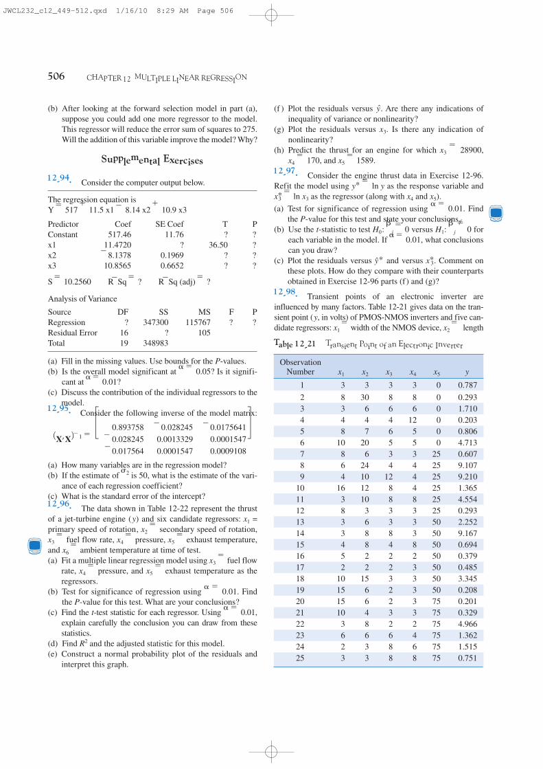
506 CHAPTER 12 MULTIPLE LINEAR REGRESSION
(b) After looking at the forward selection model in part (a),suppose you could add one more regressor to the model.This regressor will reduce the error sum of squares to 275.Will the addition of this variable improve the model? Why?
Supplemental Exercises
12-94. Consider the computer output below.
The regression equation isY ϭ 517 ϩ 11.5 x1 Ϫ 8.14 x2 ϩ 10.9 x3
Predictor Coef SE Coef T PConstant 517.46 11.76 ? ?x1 11.4720 ? 36.50 ?x2 Ϫ8.1378 0.1969 ? ?x3 10.8565 0.6652 ? ?
S ϭ 10.2560 RϪSq ϭ ? RϪSq (adj) ϭ ?
Analysis of Variance
Source DF SS MS F PRegression ? 347300 115767 ? ?Residual Error 16 ? 105Total 19 348983
(a) Fill in the missing values. Use bounds for the P-values.(b) Is the overall model significant at ␣ ϭ 0.05? Is it signifi-
cant at ␣ ϭ 0.01?(c) Discuss the contribution of the individual regressors to the
model.12-95. Consider the following inverse of the model matrix:
(a) How many variables are in the regression model?(b) If the estimate of 2 is 50, what is the estimate of the vari-
ance of each regression coefficient?(c) What is the standard error of the intercept?12-96. The data shown in Table 12-22 represent the thrustof a jet-turbine engine (y) and six candidate regressors: x1 =primary speed of rotation, x2 ϭ secondary speed of rotation,x3 ϭ fuel flow rate, x4 ϭ pressure, x5 ϭ exhaust temperature,and x6 ϭ ambient temperature at time of test.(a) Fit a multiple linear regression model using x3 ϭ fuel flow
rate, x4 ϭ pressure, and x5 ϭ exhaust temperature as theregressors.
(b) Test for significance of regression using ␣ ϭ 0.01. Findthe P-value for this test. What are your conclusions?
(c) Find the t-test statistic for each regressor. Using ␣ ϭ 0.01,explain carefully the conclusion you can draw from thesestatistics.
(d) Find R2 and the adjusted statistic for this model.(e) Construct a normal probability plot of the residuals and
interpret this graph.
1X¿X2Ϫ1 ϭ £ 0.893758Ϫ0.028245Ϫ0.017564
Ϫ0.0282450.00133290.0001547
Ϫ0.01756410.00015470.0009108
§
(f ) Plot the residuals versus Are there any indications ofinequality of variance or nonlinearity?
(g) Plot the residuals versus x3. Is there any indication of nonlinearity?
(h) Predict the thrust for an engine for which x3 ϭ 28900, x4 ϭ 170, and x5 ϭ 1589.
12-97. Consider the engine thrust data in Exercise 12-96.Refit the model using as the response variable and
ϭ ln x3 as the regressor (along with x4 and x5).(a) Test for significance of regression using ␣ ϭ 0.01. Find
the P-value for this test and state your conclusions.(b) Use the t-statistic to test H0: j ϭ 0 versus H1: j � 0 for
each variable in the model. If ␣ ϭ 0.01, what conclusionscan you draw?
(c) Plot the residuals versus and versus . Comment onthese plots. How do they compare with their counterpartsobtained in Exercise 12-96 parts (f ) and (g)?
12-98. Transient points of an electronic inverter areinfluenced by many factors. Table 12-21 gives data on the tran-sient point (y, in volts) of PMOS-NMOS inverters and five can-didate regressors: x1 ϭ width of the NMOS device, x2 ϭ length
x*3y*
x*3y* ϭ ln y
y.
Observation Number x1 x2 x3 x4 x5 y
1 3 3 3 3 0 0.7872 8 30 8 8 0 0.2933 3 6 6 6 0 1.7104 4 4 4 12 0 0.2035 8 7 6 5 0 0.8066 10 20 5 5 0 4.7137 8 6 3 3 25 0.6078 6 24 4 4 25 9.1079 4 10 12 4 25 9.210
10 16 12 8 4 25 1.36511 3 10 8 8 25 4.55412 8 3 3 3 25 0.29313 3 6 3 3 50 2.25214 3 8 8 3 50 9.16715 4 8 4 8 50 0.69416 5 2 2 2 50 0.37917 2 2 2 3 50 0.48518 10 15 3 3 50 3.34519 15 6 2 3 50 0.20820 15 6 2 3 75 0.20121 10 4 3 3 75 0.32922 3 8 2 2 75 4.96623 6 6 6 4 75 1.36224 2 3 8 6 75 1.51525 3 3 8 8 75 0.751
Table 12-21 Transient Point of an Electronic Inverter
JWCL232_c12_449-512.qxd 1/16/10 8:29 AM Page 506

12-6 ASPECTS OF MULTIPLE REGRESSION MODELING 507
Table 12-22 Thrust of a Jet-Turbine Engine
Observation Number y x1 x2 x3 x4 x5 x6
1 4540 2140 20640 30250 205 1732 992 4315 2016 20280 30010 195 1697 1003 4095 1905 19860 29780 184 1662 974 3650 1675 18980 29330 164 1598 975 3200 1474 18100 28960 144 1541 976 4833 2239 20740 30083 216 1709 877 4617 2120 20305 29831 206 1669 878 4340 1990 19961 29604 196 1640 879 3820 1702 18916 29088 171 1572 85
10 3368 1487 18012 28675 149 1522 8511 4445 2107 20520 30120 195 1740 10112 4188 1973 20130 29920 190 1711 10013 3981 1864 19780 29720 180 1682 10014 3622 1674 19020 29370 161 1630 10015 3125 1440 18030 28940 139 1572 10116 4560 2165 20680 30160 208 1704 9817 4340 2048 20340 29960 199 1679 9618 4115 1916 19860 29710 187 1642 9419 3630 1658 18950 29250 164 1576 9420 3210 1489 18700 28890 145 1528 9421 4330 2062 20500 30190 193 1748 10122 4119 1929 20050 29960 183 1713 10023 3891 1815 19680 29770 173 1684 10024 3467 1595 18890 29360 153 1624 9925 3045 1400 17870 28960 134 1569 10026 4411 2047 20540 30160 193 1746 9927 4203 1935 20160 29940 184 1714 9928 3968 1807 19750 29760 173 1679 9929 3531 1591 18890 29350 153 1621 9930 3074 1388 17870 28910 133 1561 9931 4350 2071 20460 30180 198 1729 10232 4128 1944 20010 29940 186 1692 10133 3940 1831 19640 29750 178 1667 10134 3480 1612 18710 29360 156 1609 10135 3064 1410 17780 28900 136 1552 10136 4402 2066 20520 30170 197 1758 10037 4180 1954 20150 29950 188 1729 9938 3973 1835 19750 29740 178 1690 9939 3530 1616 18850 29320 156 1616 9940 3080 1407 17910 28910 137 1569 100
JWCL232_c12_449-512.qxd 1/16/10 8:29 AM Page 507

508 CHAPTER 12 MULTIPLE LINEAR REGRESSION
of the NMOS device, x3 ϭ width of the PMOS device, x4 ϭ
length of the PMOS device, and x5 ϭ temperature (°C).(a) Fit a multiple linear regression model that uses all regres-
sors to these data. Test for significance of regression using␣ ϭ 0.01. Find the P-value for this test and use it to drawyour conclusions.
(b) Test the contribution of each variable to the model usingthe t-test with ␣ ϭ 0.05. What are your conclusions?
(c) Delete x5 from the model. Test the new model for signifi-cance of regression. Also test the relative contribution ofeach regressor to the new model with the t-test. Using ␣ ϭ 0.05, what are your conclusions?
(d) Notice that the MSE for the model in part (c) is smallerthan the MSE for the full model in part (a). Explain whythis has occurred.
(e) Calculate the studentized residuals. Do any of these seemunusually large?
(f ) Suppose that you learn that the second observation wasrecorded incorrectly. Delete this observation and refit themodel using x1, x2, x3, and x4 as the regressors. Notice thatthe R2 for this model is considerably higher than the R2 foreither of the models fitted previously. Explain why the R2
for this model has increased.(g) Test the model from part (f ) for significance of regression
using ␣ ϭ 0.05. Also investigate the contribution of eachregressor to the model using the t-test with ␣ ϭ 0.05.What conclusions can you draw?
(h) Plot the residuals from the model in part (f ) versus andversus each of the regressors x1, x2, x3, and x4. Commenton the plots.
12-99. Consider the inverter data in Exercise 12-98. Deleteobservation 2 from the original data. Define new variables asfollows: and (a) Fit a regression model using these transformed regressors
(do not use x5).(b) Test the model for significance of regression using ␣ ϭ 0.05.
Use the t-test to investigate the contribution of each vari-able to the model (␣ ϭ 0.05). What are your conclusions?
(c) Plot the residuals versus and versus each of the trans-formed regressors. Comment on the plots.
12-100. Following are data on y ϭ green liquor (g/l) and x ϭ paper machine speed (feet per minute) from a Kraft papermachine. (The data were read from a graph in an article in theTappi Journal, March 1986.)
y*
x*4 ϭ 1x4.x2* ϭ 1x2, x 3* ϭ 1ր1x3,y* ϭ ln y, x1* ϭ 1ր1x1,
y
(b) Test for significance of regression using ␣ ϭ 0.05. Whatare your conclusions?
(c) Test the contribution of the quadratic term to the model,over the contribution of the linear term, using an F-statistic.If ␣ ϭ 0.05, what conclusion can you draw?
(d) Plot the residuals from the model in part (a) versus .Does the plot reveal any inadequacies?
(e) Construct a normal probability plot of the residuals.Comment on the normality assumption.
12-101. Consider the jet engine thrust data in Exercise12-96 and 12-97. Define the response and regressors as inExercise 12-97.(a) Use all possible regressions to select the best regression
equation, where the model with the minimum value ofMSE is to be selected as “best.’’
(b) Repeat part (a) using the CP criterion to identify the bestequation.
(c) Use stepwise regression to select a subset regression model.(d) Compare the models obtained in parts (a), (b), and (c) above.(e) Consider the three-variable regression model. Calculate
the variance inflation factors for this model. Would youconclude that multicollinearity is a problem in this model?
12-102. Consider the electronic inverter data in Exercise 12-98 and 12-99. Define the response and regressors variablesas in Exercise 12-99, and delete the second observation in thesample.(a) Use all possible regressions to find the equation that min-
imizes Cp.(b) Use all possible regressions to find the equation that
minimizes MSE.(c) Use stepwise regression to select a subset regression model.(d) Compare the models you have obtained.12-103. A multiple regression model was used to relate y ϭ
viscosity of a chemical product to x1 ϭ temperature and x2 ϭ
reaction time. The data set consisted of n ϭ 15 observations.(a) The estimated regression coefficients were
and . Calculate an estimate ofmean viscosity when x1 ϭ 100°F and x2 ϭ 2 hours.
(b) The sums of squares were SST ϭ 1230.50 and SSE ϭ
120.30. Test for significance of regression using ␣ ϭ
0.05. What conclusion can you draw?(c) What proportion of total variability in viscosity is
accounted for by the variables in this model?(d) Suppose that another regressor, x3 ϭ stirring rate, is added
to the model. The new value of the error sum of squares isSSE ϭ 117.20. Has adding the new variable resulted in asmaller value of MSE? Discuss the significance of this result.
(e) Calculate an F-statistic to assess the contribution of x3 to themodel. Using ␣ ϭ 0.05, what conclusions do you reach?
12-104. Tables 12-23 and 12-24 present statistics for the MajorLeague Baseball 2005 season (source: The Sports Network).(a) Consider the batting data. Use model-building methods to
predict Wins from the other variables. Check that theassumptions for your model are valid.
2 ϭ 10.401 ϭ 0.85,0 ϭ 300.00,
y
y 16.0 15.8 15.6 15.5 14.8
x 1700 1720 1730 1740 1750
y 14.0 13.5 13.0 12.0 11.0
x 1760 1770 1780 1790 1795
(a) Fit the model using least squares.Y ϭ 0 ϩ 1x ϩ 2x2 ϩ ⑀
JWCL232_c12_449-512.qxd 1/16/10 8:29 AM Page 508

12-6 ASPECTS OF MULTIPLE REGRESSION MODELING 509
Table 12-23 Major League Baseball 2005 Season
American League BattingTeam W AVG R H 2B 3B HR RBI BB SO SB GIDP LOB OBP
Chicago 99 0.262 741 1450 253 23 200 713 435 1002 137 122 1032 0.322Boston 95 0.281 910 1579 339 21 199 863 653 1044 45 135 1249 0.357LA Angels 95 0.27 761 1520 278 30 147 726 447 848 161 125 1086 0.325New York 95 0.276 886 1552 259 16 229 847 637 989 84 125 1264 0.355Cleveland 93 0.271 790 1522 337 30 207 760 503 1093 62 128 1148 0.334Oakland 88 0.262 772 1476 310 20 155 739 537 819 31 148 1170 0.33Minnesota 83 0.259 688 1441 269 32 134 644 485 978 102 155 1109 0.323Toronto 80 0.265 775 1480 307 39 136 735 486 955 72 126 1118 0.331Texas 79 0.267 865 1528 311 29 260 834 495 1112 67 123 1104 0.329Baltimore 74 0.269 729 1492 296 27 189 700 447 902 83 145 1103 0.327Detroit 71 0.272 723 1521 283 45 168 678 384 1038 66 137 1077 0.321Seattle 69 0.256 699 1408 289 34 130 657 466 986 102 115 1076 0.317Tampa Bay 67 0.274 750 1519 289 40 157 717 412 990 151 133 1065 0.329Kansas City 56 0.263 701 1445 289 34 126 653 424 1008 53 139 1062 0.32
National League BattingTeam W AVG R H 2B 3B HR RBI BB SO SB GIDP LOB OBP
St. Louis 100 0.27 805 1494 287 26 170 757 534 947 83 127 1152 0.339Atlanta 90 0.265 769 1453 308 37 184 733 534 1084 92 146 1114 0.333Houston 89 0.256 693 1400 281 32 161 654 481 1037 115 116 1136 0.322Philadelphia 88 0.27 807 1494 282 35 167 760 639 1083 116 107 1251 0.348Florida 83 0.272 717 1499 306 32 128 678 512 918 96 144 1181 0.339New York 83 0.258 722 1421 279 32 175 683 486 1075 153 103 1122 0.322San Diego 82 0.257 684 1416 269 39 130 655 600 977 99 122 1220 0.333Milwaukee 81 0.259 726 1413 327 19 175 689 531 1162 79 137 1120 0.331Washington 81 0.252 639 1367 311 32 117 615 491 1090 45 130 1137 0.322Chicago 79 0.27 703 1506 323 23 194 674 419 920 65 131 1133 0.324Arizona 77 0.256 696 1419 291 27 191 670 606 1094 67 132 1247 0.332San Francisco 75 0.261 649 1427 299 26 128 617 431 901 71 147 1093 0.319Cincinnati 73 0.261 820 1453 335 15 222 784 611 1303 72 116 1176 0.339Los Angeles 71 0.253 685 1374 284 21 149 653 541 1094 58 139 1135 0.326Colorado 67 0.267 740 1477 280 34 150 704 509 1103 65 125 1197 0.333Pittsburgh 67 0.259 680 1445 292 38 139 656 471 1092 73 130 1193 0.322
BattingW WinsAVG Batting averageR RunsH Hits2B Doubles3B TriplesHR Home runsRBI Runs batted inBB WalksSO StrikeoutsSB Stolen basesGIDP Grounded into double play
LOB Left on baseOBP On-base percentage
PitchingERA Earned run averageSV SavesH HitsR RunsER Earned runsHR Home runsBB WalksSO StrikeoutsAVG Opponent batting average
JWCL232_c12_449-512.qxd 1/16/10 8:29 AM Page 509

Table 12-24 Major League Baseball 2005 Season
American League PitchingTeam W ERA SV H R ER HR BB SO AVG
Chicago 99 3.61 54 1392 645 592 167 459 1040 0.249Boston 95 4.74 38 1550 805 752 164 440 959 0.276LA Angels 95 3.68 54 1419 643 598 158 443 1126 0.254New York 95 4.52 46 1495 789 718 164 463 985 0.269Cleveland 93 3.61 51 1363 642 582 157 413 1050 0.247Oakland 88 3.69 38 1315 658 594 154 504 1075 0.241Minnesota 83 3.71 44 1458 662 604 169 348 965 0.261Toronto 80 4.06 35 1475 705 653 185 444 958 0.264Texas 79 4.96 46 1589 858 794 159 522 932 0.279Baltimore 74 4.56 38 1458 800 724 180 580 1052 0263Detroit 71 4.51 37 1504 787 719 193 461 907 0.272Seattle 69 4.49 39 1483 751 712 179 496 892 0.268Tampa Bay 67 5.39 43 1570 936 851 194 615 949 0.28Kansas City 56 5.49 25 1640 935 862 178 580 924 0.291
National League PitchingTeam W ERA SV H R ER HR BB SO AVG
St. Louis 100 3.49 48 1399 634 560 153 443 974 0.257Atlanta 90 3.98 38 1487 674 639 145 520 929 0.268Houston 89 3.51 45 1336 609 563 155 440 1164 0.246Philadelphia 88 4.21 40 1379 726 672 189 487 1159 0.253Florida 83 4.16 42 1459 732 666 116 563 1125 0.266New York 83 3.76 38 1390 648 599 135 491 1012 0.255San Diego 82 4.13 45 1452 726 668 146 503 1133 0.259Milwaukee 81 3.97 46 1382 697 635 169 569 1173 0.251Washington 81 3.87 51 1456 673 627 140 539 997 0.262Chicago 79 4.19 39 1357 714 671 186 576 1256 0.25Arizona 77 4.84 45 1580 856 783 193 537 1038 0.278San Francisco 75 4.33 46 1456 745 695 151 592 972 0.263Cincinnati 73 5.15 31 1657 889 820 219 492 955 0.29Los Angeles 71 4.38 40 1434 755 695 182 471 1004 0.263Colorado 67 5.13 37 1600 862 808 175 604 981 0.287Pittsburgh 67 4.42 35 1456 769 706 162 612 958 0.267
BattingW WinsAVG Batting averageR RunsH Hits2B Doubles3B TriplesHR Home runsRBI Runs batted inBB WalksSO StrikeoutsSB Stolen basesGID Grounded into double play
LOB Left on baseOBP On-base percentage
PitchingERA Earned run averageSV SavesH HitsR RunsER Earned runsHR Home runsBB WalksSO StrikeoutsAVG Opponent batting average
510 CHAPTER 12 MULTIPLE LINEAR REGRESSION
JWCL232_c12_449-512.qxd 1/16/10 8:29 AM Page 510

12-6 ASPECTS OF MULTIPLE REGRESSION MODELING 511
(b) Repeat part (a) for the pitching data.(c) Use both the batting and pitching data to build a model to
predict Wins. What variables are most important? Checkthat the assumptions for your model are valid.
12-105. An article in the Journal of the American CeramicsSociety (1992, Vol. 75, pp. 112–116) describes a process forimmobilizing chemical or nuclear wastes in soil by dissolvingthe contaminated soil into a glass block. The authors mix CaOand Na2O with soil and model viscosity and electrical conduc-tivity. The electrical conductivity model involves six regres-sors, and the sample consists of n ϭ 14 observations.(a) For the six-regressor model, suppose that SST ϭ 0.50 and
R2 ϭ 0.94. Find SSE and SSR, and use this information totest for significance of regression with ␣ ϭ 0.05. What areyour conclusions?
(b) Suppose that one of the original regressors is deleted fromthe model, resulting in R2 ϭ 0.92. What can you concludeabout the contribution of the variable that was removed?Answer this question by calculating an F-statistic.
(c) Does deletion of the regressor variable in part (b) result ina smaller value of MSE for the five-variable model, in
comparison to the original six-variable model? Commenton the significance of your answer.
12-106. Exercise 12-5 introduced the hospital patient satis-faction survey data. One of the variables in that data set is acategorical variable indicating whether the patient is a medicalpatient or a surgical patient. Fit a model including this indica-tor variable to the data, using all three of the other regressors.Is there any evidence that the service the patient is on (medicalversus surgical) has an impact on the reported satisfaction?12-107. Consider the inverse model matrix shown below.
(a) How many regressors are in this model?(b) What was the sample size?(c) Notice the special diagonal structure of the matrix. What
does that tell you about the columns in the original X matrix?
1X¿X2Ϫ1 ϭ ≥ 0.125 0 0 00 0.125 0 00 0 0.125 00 0 0 0.125
¥
MIND-EXPANDING EXERCISES
12-108. Consider a multiple regression model with kregressors. Show that the test statistic for significance of regression can be written as
Suppose that n ϭ 20, k ϭ 4, and R2 ϭ 0.90. If ␣ ϭ 0.05,what conclusion would you draw about the relationshipbetween y and the four regressors?12-109. A regression model is used to relate a responsey to k ϭ 4 regressors with n ϭ 20. What is the smallestvalue of R2 that will result in a significant regression if␣ ϭ 0.05? Use the results of the previous exercise. Areyou surprised by how small the value of R2 is?12-110. Show that we can express the residuals froma multiple regression model as e ϭ (I Ϫ H)y, where H ϭ X(X X)Ϫ1X .12-111. Show that the variance of the ith residual ei ina multiple regression model is and that thecovariance between ei and ej is Ϫ2hij, where the h’s arethe elements of H ϭ X(X X)Ϫ1X .12-112. Consider the multiple linear regression modely ϭ X ϩ ⑀. If denotes the least squares estimator of, show that where .12-113. Constrained Least Squares. Suppose wewish to find the least squares estimator of  in the model
y ϭ X ϩ ⑀ subject to a set of equality constraints, say,T ϭ c.
(a) Show that the estimator is
ϫ T[T(XX)–1T]–1(c Ϫ T )
where ϭ (XX)–1Xy.(b) Discuss situations where this model might be
appropriate.12-114. Piecewise Linear Regression. Suppose thaty is piecewise linearly related to x. That is, different lin-ear relationships are appropriate over the intervals
and .(a) Show how indicator variables can be used to fit such
a piecewise linear regression model, assuming thatthe point is known.
(b) Suppose that at the point a discontinuity occursin the regression function. Show how indicator vari-ables can be used to incorporate the discontinuityinto the model.
(c) Suppose that the point x* is not known with cer-tainty and must be estimated. Suggest an approachthat could be used to fit the piecewise linearregression model.
x*x*
x* Ͻ x Ͻ ϱϪϱ Ͻ x Յ x*


c ϭ  ϩ 1X¿X2Ϫ1
R ϭ 1X¿X2Ϫ1X¿ ϭ  ϩ R⑀,
¿
2 11 Ϫ hii2¿¿
F0 ϭR2րk11 Ϫ R2 2 ր 1n Ϫ k Ϫ 12
JWCL232_c12_449-512.qxd 1/16/10 8:29 AM Page 511

IMPORTANT TERMS AND CONCEPTS
All possible regressions
Analysis of variance test
in multiple regression
Categorical variables
Confidence interval on
the mean response
Cp statistic
Extra sum of squares
method
Hidden extrapolation
Indicator variables
Inference (test and
intervals) on individ-
ual model parameters
Influential observations
Model parameters and
their interpretation
in multiple
regression
Multicollinearity
Multiple Regression
Outliers
Polynomial regression
model
Prediction interval on a
future observation
PRESS statistic
Residual analysis and
model adequacy
checking
Significance of
regression
Stepwise regression and
related methods
Variance Inflation
Factor (VIF)
512 CHAPTER 12 MULTIPLE LINEAR REGRESSION
JWCL232_c12_449-512.qxd 1/16/10 8:29 AM Page 512