Justin Dauwels LIDS, MIT Amari Research Unit, Brain Science Institute, RIKEN June 11, 2008
Upload
scott-chenCategory
view
21download
0description

Machine learning techniques for quantifying neural synchrony: application to the diagnosis of
Alzheimer's disease from EEG
Justin DauwelsLIDS, MIT
Amari Research Unit, Brain Science Institute, RIKEN
June 11, 2008

AcknowledgmentsCollaboratorsFrançois Vialatte*, Theo Weber+, Shun-ichi Amari*, Andrzej Cichocki* (*RIKEN, +MIT)
Financial Support
•RIKEN Wako Campus (near Tokyo)
• about 400 researchers and staff (20% foreign)
• 300 research fellows and visiting scientists
• about 60 laboratories
• research covers most aspects of brain science

Overview
Alzheimer’s Disease (AD) EEG of AD patients: decrease in synchrony Synchrony measure in time-frequency domain
Pairs of EEG signalsCollections of EEG signals
Numerical Results Outlook

Alzheimer's diseaseOutside glimpse: clinical perspective
• Mild (early stage)- becomes less energetic or spontaneous- noticeable cognitive deficits- still independent (able to compensate)
• Moderate (middle stage)- Mental abilities decline- personality changes- become dependent on caregivers
• Severe (late stage)- complete deterioration of the personality- loss of control over bodily functions- total dependence on caregivers
Apathy
Memory(forgettingrelatives)
Evolution of the disease (stages)One disease,
many symptoms
Loss ofSelf-control
Video sources: Alzheimer society
• 2 to 5 years before- mild cognitive impairment (often unnoticed)- 6 to 25 % progress to Alzheimer's per year
memory, language, executive functions, apraxia, apathy, agnosia, etc…
• 2% to 5% of people over 65 years old• up to 20% of people over 80 Jeong 2004 (Nature)

Alzheimer's diseaseInside glimpse: brain atrophy
Video source: P. Thompson, J.Neuroscience, 2003
Images: Jannis Productions.(R. Fredenburg; S. Jannis)
amyloid plaques andneurofibrillary tangles
Video source: Alzheimer society

Overview
Alzheimer’s Disease (AD) EEG of AD patients: decrease in synchrony Synchrony measure in time-frequency domain
Pairs of EEG signalsCollections of EEG signals
Numerical Results Outlook

Alzheimer's diseaseInside glimpse: abnormal EEG
• AD vs. MCI (Hogan et al. 203; Jiang et al., 2005)• AD vs. Control (Hermann, Demilrap, 2005, Yagyu et al. 1997; Stam et al., 2002; Babiloni et al. 2006)• MCI vs. mildAD (Babiloni et al., 2006).
Decrease of synchrony
Brain “slow-down”
slow rhythms (0.5-8 Hz) fast rhythms (8-30 Hz)
(Babiloni et al., 2004; Besthorn et al., 1997; Jelic et al. 1996, Jeong 2004; Dierks et al., 1993).
Images: www.cerebromente.org.br
EEG system: inexpensive, mobile, useful for screening
focus of this project

Spontaneous EEG
Fourier power
f (Hz)
t (sec)
ampl
itude
Fourier |X(f)|2
EEG x(t)
Time-frequency |X(t,f)|2
(wavelet transform)
Time-frequency patterns(“bumps”)

Overview
Alzheimer’s Disease (AD) EEG of AD patients: decrease in synchrony Synchrony measure in time-frequency domain
Pairs of EEG signalsCollections of EEG signals
Numerical Results Outlook

Comparing EEG signals
PROBLEM I:
Signals of 3 seconds sampled at 100 Hz ( 300 samples)Time-frequency representation of one signal = about 25 000 coefficients
2 signals

Numerous neighboring pixels
Comparing EEG signals (2)
One pixel
PROBLEM II:
Shifts in time-frequency!

Sparse representation: bump model
Assumptions:Assumptions:
1. time-frequency map is suitable representation
2. oscillatory bursts (“bumps”) convey key information
Bumps
Sparse representation
F. Vialatte et al. “A machine learning approach to the analysis of time-frequency maps and its application to neural dynamics”, Neural Networks (2007).
104- 105 coefficients
about 102 parameters
t (sec)
f(Hz)
f(Hz)
t (sec)
f(Hz)
t (sec)

Similarity of bump models...
How “similar” or “synchronous” are two bump models?

... by matching bumps
y1 y2 Some bumps matchOffset between matched bumps
SIMILAR bump models if:Many matchesStrongly overlapping matches

... by matching bumps (2)
• Bumps in one model, but NOT in other → fraction of “spurious” bumps ρspur
• Bumps in both models, but with offset → Average time offset δt (delay) → Timing jitter with variance st
→ Average frequency offset δf → Frequency jitter with variance sf
Synchrony: only st and ρspur relevant
PROBLEM: Given two bump models, compute (ρspur, δt, st, δf, sf )
Stochastic Event Synchrony (SES) = (ρspur, δt, st, δf, sf )

Generative modelGenerate bump model (hidden)
• geometric prior for number n of bumps p(n) = (1- λ S) (λ S)-n
• bumps are uniformly distributed in rectangle
• amplitude, width (in t and f) all i.i.d.
Generate two “noisy” observations
• offset between hidden and observed bump = Gaussian random vector with mean ( ±δt /2, ±δf /2) covariance diag(st/2, sf /2)
• amplitude, width (in t and f) all i.i.d.
• “deletion” with probability pd
yhidden
y y’
Easily extendable to more than 2 observations…
( -δt /2, -δf /2)
( δt /2, δf /2)

Generative model (2)
• Binary variables ckk’
ckk’ = 1 if k and k’ are observations of same hidden bump, else ckk’ = 0 (e.g., cii’ = 1 cij’ = 0)
• Constraints: bk = Σk’ ckk’ and bk’ = Σk ckk’ are binary (“matching constraints”)
• Generative Model p(y, y’, yhidden , c, δt , δf , st , sf ) (symmetric in y and y’)
• Eliminate yhidden → offset is Gaussian RV with mean = ( δt , δf ) and covariance diag (st , sf)
• Probabilistic Inference:(c*,θ*) = argmaxc,θ log p(y, y’, c, θ)
y y’
( -δt /2, -δf /2)
( δt /2, δf /2)
i
i’ j’
p(y, y’, c, θ) = ∫ p(y, y’, yhidden , c, θ) dyhidden
θ

• Bumps in one model, but NOT in other → fraction of “spurious” bumps ρspur
• Bumps in both models, but with offset → Average time offset δt (delay) → Timing jitter with variance st
→ Average frequency offset δf → Frequency jitter with variance sf
PROBLEM: Given two bump models, compute (ρspur, δt, st, δf, sf )
APPROACH: (c*,θ*) = argmaxc,θ log p(y, y’, c, θ)θ
Summary
Objective function
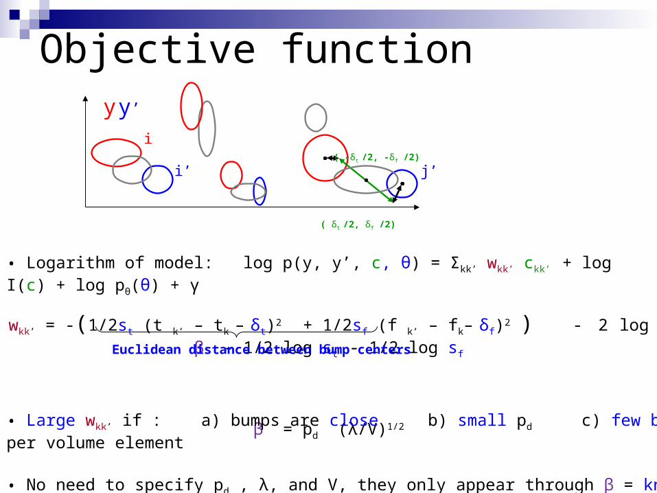
• Logarithm of model: log p(y, y’, c, θ) = Σkk’ wkk’ ckk’ + log I(c) + log pθ(θ) + γ
wkk’ = -(1/2st (t k’ – tk – δt)2 + 1/2sf (f k’ – fk– δf)2 ) - 2 log β - 1/2 log st - 1/2 log sf
β = pd (λ/V)1/2
Euclidean distance between bump centers
• Large wkk’ if : a) bumps are close b) small pd c) few bumps per volume element
• No need to specify pd , λ, and V, they only appear through β = knob to control # matches
y y’
( -δt /2, -δf /2)
( δt /2, δf /2)
i
i’ j’

p(y, y’, c, θ) / I(c) pθ(θ) Πkk’ (N(t k’ – tk ; δt ,st,kk’) N(f k’ – fk ; δf ,sf, kk’) β-2)ckk’
Generative model

Expect bumps to appear at about same frequency, but delayed
Frequency shift requires non-linear transformation, less likely than delay
Conjugate priors for st and sf (scaled inverse chi-squared):
Improper prior for δt and δt : p(δt) = 1 = p(δf)
Prior for parameters

Probabilistic inference
MATCHINGPOINT ESTIMATION
PROBLEM: Given two bump models, compute (ρspur, δt, st, δf, sf )
APPROACH: (c*,θ*) = argmaxc,θ log p(y, y’, c, θ)
θ
SOLUTION: Coordinate descent
c(i+1) = argmaxc log p(y, y’, c, θ(i) ) θ(i+1) = argmaxx log p(y, y’, c(i+1) ,θ )
X
Y
Minx2 X, y2Y d(x,y)

POINT ESTIMATION: θ(i+1) = argmaxx log p(y, y’, c(i+1) ,θ )
Uniform prior p(θ): δt, δf = average offset, st, sf = variance of offset Conjugate prior p(θ): still closed-form expressionOther kind of prior p(θ): numerical optimization (gradient method)
Probabilistic inference

MATCHING: c(i+1) = argmaxc log p(y, y’, c, θ(i) )
ALGORITHMS
• Polynomial-time algorithms gives optimal solution(s) (Edmond-Karp and Auction algorithm)• Linear programming relaxation gives optimal solution if unique [Sanghavi (2007)]• Max-product algorithm gives optimal solution if unique [Bayati et al. (2005), Sanghavi (2007)]
EQUIVALENT to (imperfect) bipartite max-weight matching problem (belongs to P)
c(i+1) = argmaxc log p(y, y’, c, θ(i) ) = argmaxc Σkk’ wkk’(i) ckk’
s.t. Σk’ ckk’ ≤ 1 and Σk ckk’ ≤ 1 with ckk’ 2 {0,1}
Probabilistic inference
not necessarily perfectfind heaviest set of disjoint edges

p(y, y’, c, θ) / I(c) pθ(θ) Πkk’ (N(t k’ – tk ; δt ,st,kk’) N(f k’ – fk ; δf ,sf, kk’) β-2)ckk’
Max-product algorithmMATCHING: c(i+1) = argmaxc log p(y, y’, c, θ(i) )
Generative model

Max-product algorithmMATCHING: c(i+1) = argmaxc log p(y, y’, c, θ(i) )
μ↑μ↑
μ↓ μ↓
Conditioning on θ

Max-product algorithm (2)• Iteratively compute messages
• At convergence, compute marginals p(ckk’) = μ↓(ckk’) μ↓(ckk’) μ↑(ckk’)
• Decisions: c*kk’ = argmaxckk’ p(ckk’)

Summary
MATCHING → max-productESTIMATION → closed-form
PROBLEM: Given two bump models, compute (ρspur, δt, st, δf, sf )
APPROACH: (c*,θ*) = argmaxc,θ log p(y, y’, c, θ)
θ
SOLUTION: Coordinate descent
c(i+1) = argmaxc log p(y, y’, c, θ(i) ) θ(i+1) = argmaxx log p(y, y’, c(i+1) ,θ )

Average synchrony
3. SES for each pair of models4. Average the SES parameters
1. Group electrodes in regions2. Bump model for each region

Overview
Alzheimer’s Disease (AD) EEG of AD patients: decrease in synchrony Synchrony measure in time-frequency domain
Pairs of EEG signalsCollections of EEG signals
Numerical Results Outlook

Beyond pairwise interactions...
Pairwise similarity Multi-variate similarity

...by clusteringy1 y2 y3 y4 y5
y1 y2 y3 y4 y5
Constraint: in each cluster at most one bump from each signal
Models similar if• few deletions/large clusters• little jitter

Generative model
Generate bump model (hidden)
• geometric prior for number n of bumps p(n) = (1- λ S) (λ S)-n
• bumps are uniformly distributed in rectangle
• amplitude, width (in t and f) all i.i.d.
Generate M “noisy” observations
• offset between hidden and observed bump = Gaussian random vector with mean ( δt,m /2, δf,m /2) covariance diag(st,m/2, sf,m /2)
• amplitude, width (in t and f) all i.i.d.
• “deletion” with probability pd
yhidden
y1 y2 y3 y4 y5
Parameters: θ = δt,m , δf,m , st,m , sf,m, pc
pc (i) = p(cluster size = i |y) (i = 1,2,…,M)

Inference• SOLUTION 1
ITERATE:• Infer hidden bump model (= cluster centers)• Compute parameters δt,m , δf,m , st,m , sf,m, pc
= adaption of K-means clustering= ESTIMATION problem
PROBLEM: LOCAL extrema!
• SOLUTION 2Assumption: one bump in each cluster is hidden bump (“exemplar”)ITERATE:
• Find exemplars (= cluster centers) and non-exemplars • Compute parameters δt,m , δf,m , st,m , sf,m, pc
= DETECTION problem (combinatorial optimization/integer program)= adaption of “affinity propagation” [Frey et al., Science, 2007] or convex clustering algorithm [Lashkari et al., NIPS 2007]
ADVANTAGE: we can find GLOBAL OPTIMUM!

Exemplar-based formulationyhidden
y1 y2 y3 y4 y5
Parameters: θ = δt,m , δf,m , st,m , sf,m, pc
pc (i) = p(cluster size = i |y) (i = 1,2,…,M)
Set of EXEMPLARS = “average” point process → compression

Exemplar-based formulation: IPBinary Variables
Integer Program: LINEAR objective function/constraints
Equivalent to k-dim matching: for k = 2: in P but for k > 2: NP-hard!

Probabilistic inference
CLUSTERING (IP or MP)POINT ESTIMATION
PROBLEM: Given M bump models, compute θ = δt,m , δf,m , st,m , sf,m, pc
APPROACH: (b*,θ*) = argmaxc,θ log p(y, y’, b, θ)
SOLUTION: Coordinate descent
b(i+1) = argmaxc log p(y, y’, b, θ(i) ) θ(i+1) = argmaxx log p(y, y’, b(i+1) ,θ )
Integer program• Max-product algorithm (MP) on sparse graph: FAILED!• Integer programming methods (e.g., LP relaxation): GREAT!
• IP with 10.000 variables solved in about 1s, total run time about 5s• CPLEX: commercial toolbox for solving IPs (combines several algorithms)

Overview
Alzheimer’s Disease (AD) EEG of AD patients: decrease in synchrony Synchrony measure in time-frequency domain
Pairs of EEG signalsCollections of EEG signals
Numerical Results Outlook

EEG Data
EEG data provided by Prof. T. Musha
• EEG of 22 Mild Cognitive Impairment (MCI) patients and 38 age-matched control subjects (CTR) recorded while in rest with closed eyes → spontaneous EEG
• All 22 MCI patients suffered from Alzheimer’s disease (AD) later on
• Electrodes located on 21 sites according to 10-20 international system
• Electrodes grouped into 5 zones (reduces number of pairs) 1 bump model per zone
• Used continuous “artifact-free” intervals of 20s
• Band pass filtered between 4 and 30 Hz

Similarity measures• Correlation and coherence• Granger causality (linear system): DTF, ffDTF, dDTF, PDC, PC, ...
• Phase Synchrony: compare instantaneous phases (wavelet/Hilbert transform)
• State space based measures sync likelihood, S-estimator, S-H-N-indices, ...
• Information-theoretic measures KL divergence, Jensen-Shannon divergence, ...
No Phase Locking Phase Locking
TIME FREQUENCY


Sensitivity (average synchrony)
Granger
Info. Theor.
State Space
Phase
SES
Corr/Coh
Mann-Whitney test: small p value suggests large difference in statistics of both groups
Significant differences for ffDTF and ρ!

Classification
• Clear separation, but not yet useful as diagnostic tool• Additional indicators needed (fMRI, MEG, DTI, ...)• Can be used for screening population (inexpensive, simple, fast)
ffDTF

Strong (anti-) correlations „families“ of sync measures
Correlations

Recent results for multivariate SES
SMALLER clusters in MCI patients!
Cluster size = 1 Cluster size = 2
Cluster size = 3 Cluster size = 4
Cluster size = 5

Recent results for multivariate SES (2)
± 90% correctly classified
± 85% correctly classified
Average cluster size
Average cluster size

Overview
Alzheimer’s Disease (AD) EEG of AD patients: decrease in synchrony Synchrony measure in time-frequency domain
Pairs of EEG signalsCollections of EEG signals
Numerical Results Ongoing Work and Outlook

Ongoing work Time-varying similarity parameters
st
low st high sthigh st
no stimulus no stimulusstimulus
low st high sthigh st

Probabilistic inference
CLUSTERING (IP or MP)CUBIC SPLINE SMOOTHING
PROBLEM: Given M bump models, compute θ = δt,m , δf,m , st,m , sf,m, pc
APPROACH: (b*,θ*) = argmaxc,θ log p(y, y’, b, θ)
SOLUTION: Coordinate descent
b(i+1) = argmaxc log p(y, y’, b, θ(i) ) θ(i+1) = argmaxx log p(y, y’, b(i+1) ,θ )
PRIOR:
POINT ESTIMATION:

Future work
yhidden
y1 y2 y3 y4 y5
Less trivial prior (not i.i.d.)Multiple hidden processes
- independent- dependent
More complex transformations = “observation model”
MODEL
INFERENCE: infer distributions instead of point estimates

Conclusions
Measure for similarity of point processes („stochastic event synchrony“)
Key idea: alignment of events
Solved by statistical inference
Application: EEG synchrony of MCI patients
About 85-90% correctly classified; perhaps useful for screening population
Ongoing/future work: more complex models, more detailed inference

Machine learning techniques for quantifying neural synchrony: application to the diagnosis of
Alzheimer's disease from EEG
Justin DauwelsLIDS, MIT
Amari Research Unit, Brain Science Institute, RIKEN
June 11, 2008

Machine learning for neuroscience
Multi-scale in time and space
Data fusion: EEG, fMRI, dMRI, spike data, bio-imaging, ...
Large-scale inference
Visualization
Behavior ↔ Brain ↔ Brain Regions ↔ Neural Assemblies ↔ Single neurons ↔ Synapses ↔ Ion channels

Research Overview
• EEG (RIKEN, MIT, MGH, MPI)• diagnosis of Alzheimer’s disease• detection/prediction of epileptic seizures• analysis of EEG evoked by visual/auditory stimuli• EEG during meditation• projects related to brain-computer interface (BMI)
• Calcium imaging (RIKEN, NAIST, MIT)•role of calcium in neural growth•role of calcium propagation in gliacells and neurons
• Diffusion MRI (Brigham&Women’s Hospital, Harvard Medical School, MIT)
• estimation and clustering of tracts
Machine learning & signal processing for applications in NEUROSCIENCE = development of ALGORITHMS to analyze brain signals
subject of this talk

Signatures of local synchronyf (Hz)
t (sec)
Time-frequency patterns(“bumps”)
EEG stems from thousands of neuronsbump if neurons are phase-locked= local synchrony

Distance measures
wkk’ = 1/st,kk’ (t k’ – tk – δt)2 + 1/sf,kk’ (f k’ – fk– δf)2 + 2 log β
st,kk’ = (Δtk + Δt’k) st sf,kk’ = (Δfk + Δf’k) sf
Scaling
Non-Euclidean

Future work: MODELyhidden
y1 y2 y3 y4 y5
Less trivial prior (not i.i.d.)Multiple hidden processes
- independent- dependent
More complex transformations = “observation model”

Illustration Matching event patterns instead of single events
= allows us to extract patterns in time-frequency map of EEG!
HYPOTHESIS:Perhaps specific patterns occur in time-frequency EEG maps of AD patients before onset of epileptic seizures
REMARK:Such patterns are ignored by classical approaches: STATIONARITY/AVERAGING!
coupling betweenfrequency bands
t (sec)
f(Hz)

Probabilistic inferencePOINT ESTIMATION:
SOLUTION 1: Solve EULER-LAGRANGE equations numerically (Runge-Kutta) PROBLEM 1: Slow! PROBLEM 2: Need to optimize over initial value…
SOLUTION 2: OBSERVATION: solution of (1) = cubic splines - bring (2) in the form (1) = Laplace or saddle-point approximation - solve (1) and (2) iteratively using cubic-spline smoothing
ADVANTAGE 1: Fast! ADVANTAGE 2: Just a few lines of code
(1)
(2)

Probabilistic inference
CLUSTERING (IP or MP)CUBIC SPLINE SMOOTHING
PROBLEM: Given M bump models, compute θ = δt,m , δf,m , st,m , sf,m, pc
APPROACH: (b*,θ*) = argmaxc,θ log p(y, y’, b, θ)
SOLUTION: Coordinate descent
b(i+1) = argmaxc log p(y, y’, b, θ(i) ) θ(i+1) = argmaxx log p(y, y’, b(i+1) ,θ )

Probabilistic inferencePOINT ESTIMATION:
SOLUTION 1: Solve EULER-LAGRANGE equations numerically (Runge-Kutta) PROBLEM 1: Slow! PROBLEM 2: Need to optimize over initial value…
SOLUTION 2: OBSERVATION: solution of (1) = cubic splines - bring (2) in the form (1) = Laplace or saddle-point approximation - solve (1) and (2) iteratively using cubic-spline smoothing
ADVANTAGE 1: Fast! ADVANTAGE 2: Just a few lines of code
(1)
(2)

Future work (2): INFERENCE
Combination of two ideas:
• Non-stationary Gaussian processes instead of splines [Plagemann et al., ECML 2008]
• Hierarchical dirichlet processes instead of IP formulation inference by Gibbs sampling (project with E. Fox and A. Willsky)
Full bayesian treatment = infer distributions instead of point estimates

Future work: MODELyhidden
y1 y2 y3 y4 y5
Less trivial prior (not i.i.d.)Multiple hidden processes
- independent- dependent
More complex transformations = “observation model”

Illustration Matching event patterns instead of single events
= allows us to extract patterns in time-frequency map of EEG!
HYPOTHESIS:Perhaps specific patterns occur in time-frequency EEG maps of AD patients before onset of epileptic seizures
REMARK:Such patterns are ignored by classical approaches: STATIONARITY/AVERAGING!
coupling betweenfrequency bands
t (sec)
f(Hz)

Estimation
Deltas: average offset Sigmas: var of offset
...where
Simple closed form expressions
artificial observations (conjugate prior)

Large-scale synchrony
Apparently, all brain regions affected...

Alzheimer's diseaseOutside glimpse: the future (prevalence)
USA (Hebert et al. 2003)
World (Wimo et al. 2003)
Mil
lio
n o
f su
ffer
ers
Mil
lio
n o
f su
ffer
ers
• 2% to 5% of people over 65 years old
• Up to 20% of people over 80
Jeong 2004 (Nature)

(Hebb 1949, Fuster 1997)
Stimuli Consolidation Stimulus
Voice Face Voice
Neuronal assemblies
Assembly activation Hebbian consolidationAssembly recall

Ongoing and future work
Applications
alternative inference techniques (e.g., MCMC, linear programming) time dependent (Gaussian processes) multivariate (T.Weber)
Fluctuations of EEG synchrony Caused by auditory stimuli and music (T. Rutkowski) Caused by visual stimuli (F. Vialatte) Yoga professionals (F. Vialatte) Professional shogi players (RIKEN & Fujitsu) Brain-Computer Interfaces (T. Rutkowski)
Spike data from interacting monkeys (N. Fujii) Calcium propagation in gliacells (N. Nakata) Neural growth (Y. Tsukada & Y. Sakumura) ...
Algorithms

Fitting bump models
Signal
Bump
Initialisation After adaptationAdaptation
gradient method
F. Vialatte et al. “A machine learning approach to the analysis of time-frequency maps and its application to neural dynamics”, Neural Networks (2007).

Boxplots
SURPRISE!No increase in jitter, but significantly less matched activity!
Physiological interpretation• neural assemblies more localized?• harder to establish large-scale synchrony?

Similarity of bump models...
How “similar” or “synchronous” are two bump models?

References + software
References
Quantifying Statistical Interdependence by Message Passing on Graphs: Algorithms and Application to Neural Signals, Neural Computation (under revision)
A Comparative Study of Synchrony Measures for the Early Diagnosis of Alzheimer's Disease Based on EEG, NeuroImage (under revision)
Measuring Neural Synchrony by Message Passing, NIPS 2007
Quantifying the Similarity of Multiple Multi-Dimensional Point Processes by Integer Programming with Application to Early Diagnosis of Alzheimer's Disease from EEG, EMBC 2008 (submitted)
Software
MATLAB implementation of the synchrony measures