Juniper: A Tree+Table Approach to Multivariate Graph Visualization

Carolina Nobre, Marc Streit, and Alexander Lex

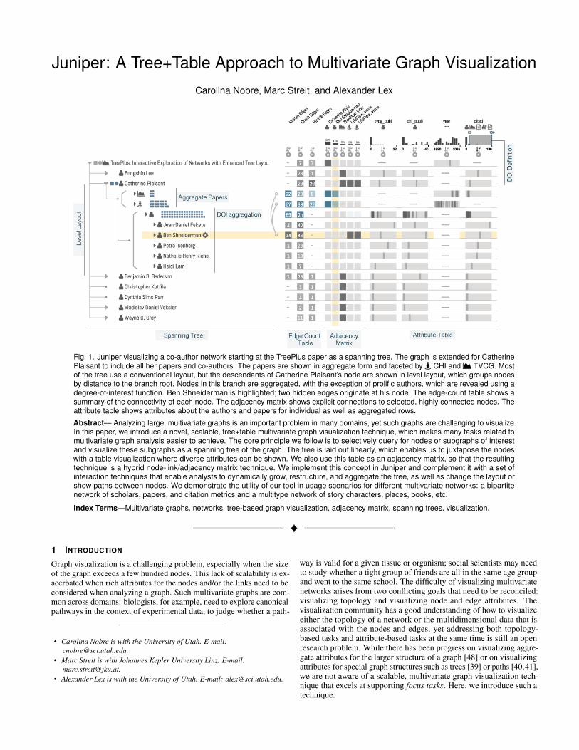
Fig. 1. Juniper visualizing a co-author network starting at the TreePlus paper as a spanning tree. The graph is extended for CatherinePlaisant to include all her papers and co-authors. The papers are shown in aggregate form and faceted by y CHI and ^ TVCG. Mostof the tree use a conventional layout, but the descendants of Catherine Plaisant’s node are shown in level layout, which groups nodesby distance to the branch root. Nodes in this branch are aggregated, with the exception of prolific authors, which are revealed using adegree-of-interest function. Ben Shneiderman is highlighted; two hidden edges originate at his node. The edge-count table shows asummary of the connectivity of each node. The adjacency matrix shows explicit connections to selected, highly connected nodes. Theattribute table shows attributes about the authors and papers for individual as well as aggregated rows.

Abstract— Analyzing large, multivariate graphs is an important problem in many domains, yet such graphs are challenging to visualize.In this paper, we introduce a novel, scalable, tree+table multivariate graph visualization technique, which makes many tasks related tomultivariate graph analysis easier to achieve. The core principle we follow is to selectively query for nodes or subgraphs of interestand visualize these subgraphs as a spanning tree of the graph. The tree is laid out linearly, which enables us to juxtapose the nodeswith a table visualization where diverse attributes can be shown. We also use this table as an adjacency matrix, so that the resultingtechnique is a hybrid node-link/adjacency matrix technique. We implement this concept in Juniper and complement it with a set ofinteraction techniques that enable analysts to dynamically grow, restructure, and aggregate the tree, as well as change the layout orshow paths between nodes. We demonstrate the utility of our tool in usage scenarios for different multivariate networks: a bipartitenetwork of scholars, papers, and citation metrics and a multitype network of story characters, places, books, etc.

Index Terms—Multivariate graphs, networks, tree-based graph visualization, adjacency matrix, spanning trees, visualization.

1 INTRODUCTION

Graph visualization is a challenging problem, especially when the sizeof the graph exceeds a few hundred nodes. This lack of scalability is ex-acerbated when rich attributes for the nodes and/or the links need to beconsidered when analyzing a graph. Such multivariate graphs are com-mon across domains: biologists, for example, need to explore canonicalpathways in the context of experimental data, to judge whether a path-

• Carolina Nobre is with the University of Utah. E-mail:cnobre@sci.utah.edu.

• Marc Streit is with Johannes Kepler University Linz. E-mail:marc.streit@jku.at.

• Alexander Lex is with the University of Utah. E-mail: alex@sci.utah.edu.

way is valid for a given tissue or organism; social scientists may needto study whether a tight group of friends are all in the same age groupand went to the same school. The difficulty of visualizing multivariatenetworks arises from two conflicting goals that need to be reconciled:visualizing topology and visualizing node and edge attributes. Thevisualization community has a good understanding of how to visualizeeither the topology of a network or the multidimensional data that isassociated with the nodes and edges, yet addressing both topology-based tasks and attribute-based tasks at the same time is still an openresearch problem. While there has been progress on visualizing aggre-gate attributes for the larger structure of a graph [48] or on visualizingattributes for special graph structures such as trees [39] or paths [40,41],we are not aware of a scalable, multivariate graph visualization tech-nique that excels at supporting focus tasks. Here, we introduce such atechnique.

We use the term focus tasks to refer to tasks where the details ofindividual nodes, edges, and their neighborhood matter, as opposedto the global structure of the network. Focus tasks commonly requirereadable labels and a detailed understanding of a node’s attributes.These tasks include identifying adjacent nodes (who are my friends?),identifying nodes that are accessible from another node (where can Ifly to from this airport within at most one layover?), finding short paths(what’s the best route to go from A to B?), etc. Examples for focusgraph tasks on multivariate networks include investigating congestionand latency in a computer network or exploring how a mutated geneinfluences activity levels of the genes in its neighborhood. It is worthnoting that these focus graph tasks are equally important in both largeand small graphs.

Our primary contribution is Juniper, a new interactive technique thatis tailored to address focus tasks when visualizing large, multivariatenetworks. The core idea is to extract a spanning tree from a subgraphthat is the result of a query of a larger graph. The spanning tree isgrown from a node of interest and laid out in a linearized tree, whereevery node can be unambiguously associated with a row in a table. Thistable is used to visualize topological properties of the tree, such as thedegree of the nodes and their adjacency to selected other nodes, and toshow rich attributes.

We also contribute an implementation of this technique, which en-riches this basic concept with user interactions to restructure the tree tobest answer the analyst’s question, expose additional topological infor-mation such as edges not included in the tree, identify shortest pathsbetween nodes, explore interdependent attributes along paths in thenetwork, aggregate groups of nodes to save space, expand the networkon demand, filter nodes by type, or sort them based on attributes.

Juniper is tailored to address focus tasks related to the details of alarge network. We argue that this class of tasks is important in manypractical applications and complementary to overview tasks that arebetter addressed with other techniques.

2 DATA AND TASKS

We consider graphs G = (N,E) with nodes n ∈ N and edges e ∈ E,which can be of different types t ∈ T . Edges can be directed. Nodeshave attributes a ∈ Anodes associated with them. Typically, nodes ofdifferent types also have different attributes. Node attributes can benumerical, ordinal, nominal, sets, or labels/identifiers. Although ourprototype does not currently support it, conceptually we could alsoincorporate edge attributes. Juniper renders a subset of the graphgsub ∈ G, where |gsub| � |G|. This subgraph is selected by an analystto satisfy a specific question and can change over the course of ananalysis. Subgraphs do not have to be connected.

Whereas many graph visualization techniques are designed to sup-port overview tasks and to be scalable with respect to the absolutenumber of nodes, edges, and attributes shown, only a few graph vi-sualization tasks require getting a large-scale overview of a network.We consider all tasks where analysts need to see a large set of nodesand edges to be overview tasks. Examples of such overview tasksare estimating the size of a network, identifying clusters, or findingarticulation points. An example for multivariate networks is to explorehow migration patterns within the US differ by age. When visualizingoverviews of all but trivial networks, the large number of nodes andedges makes it impossible to show labels and attributes for individualnodes. For focus tasks, the details of a small, well-defined subset ofnodes are relevant and necessary for the task. These details includetopological information such as neighborhoods of or paths betweennodes; and attributes, including node labels and other associated data.

To get a better sense of the importance of focus tasks, we classifiedLee et al.’s task taxonomy for graph visualization [33] into whetherthe tasks are focus tasks or require an overview. Of nine tasks Leeet al. identify, five are focus tasks (adjacency, accessibility, commonconnection, follow path, revisit). The attribute-related tasks — nodeattributes, link attributes — are described mostly in a focus context byLee et al., but they can also be useful in a global context (for example,estimating the average age of members of a social network). One task— connectivity — can be broken up into overview and focus tasks. For

example, finding the shortest path between nodes is a focus connectiv-ity task, but identifying clusters, connected components, bridges, orarticulation points is an overview variant of the connectivity task.

With regard to topology-attribute interaction, focus tasks can beclassified into two groups: (1) those that can be achieved in the contextof neighborhoods (adjacency, accessibility, common connection), e.g.,to see whether friends have similar educational attainment or whetherhealth issues, such as obesity, spread in a neighborhood of friends [5],and (2) those related to exploring attributes in the context of paths(follow path, connectivity), for example, to judge delays over time in acomputer network or whether a path in a biological pathway is activein a set of samples [41].

Juniper is designed to support focus tasks, specifically the types oftasks that are concerned with both topology and attributes. We employa bottom-up graph visualization technique [49, 50] where analysts startwith a query and expand the network on demand. As such, it is wellsuited to answer questions about specific subnetworks, but it cannotgive large-scale overviews of the network.

3 RELATED WORK

Juniper is inspired by and contributes to multiple subfields of graphvisualization. Here we discuss how our work relates to multivariategraph and tree visualization, to tree-based graph visualization, and toquery-based visualization of large graphs.

3.1 Multivariate Graph and Tree Visualization

A multivariate graph is a graph where the nodes and/or edges are asso-ciated with attributes [26]. Although most graphs have some attributes,such as a node type, multivariate graph visualization techniques areconcerned with graphs with several or even hundreds of associated at-tributes. A common goal of multivariate graph visualization techniquesis to allow analysts to jointly analyze topology and attributes and reasonabout their relationship. Partl et al. [41] discuss four different types ofmultivariate graph visualization techniques, based on node-link layouts,which we use to structure this section. We also discuss matrix-basedtechniques as a fifth type.(1) On-node encoding refers to modifying the visual appearance of anode (size, color), or embedding marks in it (bar charts, line charts,etc.) Color coding is a common choice to encode a single data valueor a node type; the latter is also often encoded using node shapes oricons. Gehlenborg et al. [13] review techniques used in systems biologyfor visualizing multivariate networks, many of which make use of on-node encoding using embedded charts, such as line charts, box plots,etc. On-node encoding is also widely supported by common graphvisualization tools such as Cytoscape [44] and Gephi [2]. Van den Elzenand van Wijk [48] use embedded visualizations to show distributionsof values aggregated in a super-node. On-node encoding supportsthe integration of topology and attribute-based tasks well; however, itcomes with scalability trade-offs. Even for a modest number of nodesin a node-link layout, node size has to be limited; hence little space isavailable to encode attributes. When details about nodes are shown,as, for example, in MoireGraphs [23], the number of nodes that can bedisplayed simultaneously is limited.(2) Multiple coordinated view (MCV) approaches use separate, ded-icated views for the attributes and the topology. Common examplesare combinations of force-directed node-link diagrams with multidi-mensional data visualization techniques [35, 43], or providing a detailview for individual nodes [18, 46]. Although this solution is flexibleand easy to implement, it requires interactive highlighting to identifyrelationships between nodes and their attributes. MCV-based attributevisualization is supported by standard graph drawing tools [2, 44].(3) Small multiples show multiple instances of the same graph layout.Each instance encodes a different attribute dimension. Small multiplespreserve the topology well, as they embed individual attributes directlyin the graph [1, 36]. Disadvantages of small multiples include difficultycomparing attributes across the views, and having to render each indi-vidual graph with little space, limiting the size of the graph that can bevisualized.

(4) Layout adaption works by adjusting the layout so that a direct asso-ciation between the nodes/edges and their attributes can be established.This is a broad category that includes placing the nodes in a scatterplotdefined by two attributes as in GraphDice [3] or aggregating nodesinto bar charts as in GraphTrail [6]. Another strategy is to linearize(parts of) a node-link layout so that it can be easily juxtaposed with atable visualizing node or edge attributes. Examples of this approachinclude Pathline [37], where a whole network including cycles andbranching is linearized and juxtaposed with an attribute visualization;enRoute [41], which linearizes a user-chosen path; and Pathfinder [40],which queries for paths in networks and juxtaposes those paths withattribute visualizations. All these approaches make compromises be-tween the readability of the topology of the graph and the associationof the attributes to the network.(5) Adjacency matrices have both favorable and unfavorable proper-ties compared to node-link layouts when judging topology [14]. Variousattempts have been made to combine node-link layouts with matricesto find a compromise between these trade-offs. Examples are Node-Trix [20], which embeds adjacency matrices for subgraphs of a node-link layout, and MatLink [19], which enhances matrices with links.For attribute visualization, however, adjacency matrices are superiorto node-link diagrams. For example, adjacency matrices can naturallyencode edge attributes in matrix cells. Although this is mostly donewith a single color value, multiple edge attributes can be visualizedas nested graphs [9]. Similar to the on-node encoding in node-linkdiagrams, however, the small space available for a matrix cell limitshow much can be encoded. For node attributes, in contrast, it is easy tojuxtapose multiple attribute visualizations with the rows or columns ofthe matrix. This has been done, for example in Graffinity [27] and inMapTrix [51].

Juniper is a layout adaption technique. It uses a linearized spanningtree to visualize a graph and juxtaposes it with a tabular visualizationtechnique. We argue that this combination hits a sweet-spot in thetopology-attribute trade-off spectrum. The linear tree-layout of thegraph enables us to also juxtapose and align it with an adjacency matrix,resulting in a hybrid node-link/matrix technique, thereby leveraging theadvantages of both: the ease of identifying paths in a node-link layoutand the ability to quickly identify neighbors in the matrix layout.

Multivariate Tree Visualization Although the data we consider isof graph form, we present the graph as a tree. Hence it is useful to alsoconsider the literature for multivariate trees in our review. Since treesare only a special type of graph, we can visualize it using any of theseapproaches.

In contrast to general graphs, trees can also be visualized usingimplicit layouts, such as tree maps [24], sunburst plots [45], or icicleplots [29]. Implicit techniques can use on-node encoding, such ascolor-coding on the node set, but they cannot be used to visualize edgeattributes, as the edges are implicit.

A large number of techniques visualize attributes of the leaves of atree in a tabular layout (a layout adaption strategy). Common examplesare cases where the tree is a dendrogram that visualizes the hierarchicalrelationship of the items in a table [7]. Similar approaches have beenused for visualizing phylogenies and attributes about the species theycontain [28, 31] or transactions associated with a hierarchy [4]. Sur-prisingly few techniques also visualize attributes for inner nodes in atree. One example is a tree-table as it is used, e.g., in file browsers,showing properties such as file types and file/directory sizes. Anotherexample is our Lineage tool [39], which is designed to visualize clinicalgenealogies. The genealogies considered in Lineage are trees that arejuxtaposed with a table that visualizes the properties of individuals. Insome sense, Juniper is a generalization of the multivariate tree visual-ization techniques introduced in Lineage to general, highly connectedgraphs. Compared to Lineage, Juniper focuses on techniques that en-able the exploration of a multivariate graph as a tree, which includescomplete control over which edges to include in the tree, visualizingselected edges in an adjacency matrix, and dynamically growing thetree from a much larger graph. Section 8 contains a detailed discussionof the differences of Juniper and Lineage.

3.2 Tree-based Graph VisualizationThe idea of tree-based graph drawing goes back at least two decades.Munzner uses a spanning tree as the structure to lay out a graph inhyperbolic space [38] and shows links that are not part of the tree ondemand. Hao et al. [17] take a similar approach, but they also introduceduplicates to resolve some ambiguities. Similarly, Ontorama [8] uses ahyperbolic layout for a spanning tree and supplements it with a secondview showing a linear tree that allows duplicate nodes.

Yee et al. [52] introduce a radial layout for graphs based on spanningtrees. A focus node is used as the root of a spanning tree and shownat the center, immediate neighbors are shown circling the focus nodes,neighbors once removed are shown on a second circle, etc. The edgesof the spanning tree and other non-tree edges are shown in a differentcolor. Animated transitions are used to dynamically update the focusnode. MoireGraphs [23] follow the same principle but combine theradial layout with rich on-node attribute visualizations.

The works most closely related to ours are TreePlus by Lee et al. [32]and the application-specific variant of TreePlus, GOTreePlus [30].TreePlus introduces the “plant a seed and watch it grow” principle.Based on an initial, user-chosen node, analysts can grow the spanningtree by successively revealing subtrees. TreePlus shows hidden linksbetween the tree nodes on demand using a combination of highlighting,a separate view of neighboring nodes, and explicit cross-links. Lee et al.evaluated TreePlus by comparing it to a traditional node-link diagramin a controlled study and found that TreePlus outperforms the node-link layout for most tasks and is preferred by most participants. For adetailed discussion of the differences of TreePlus and Juniper, refer toSection 8. Most of these techniques, including Munzner’s hyperbolictree, the radial layouts, and TreePlus, also encode node attributes, butthey limit attribute visualization to on-node encoding of one or fewattributes.

Another type of technique visualizes compound graphs that haveboth a tree and a secondary graph structure. Fekete et al. [10], forexample, visualize a tree structure in a compound graph as a tree mapand render cross-links between the tree nodes on top of it. Holten [21]uses a compound graph as an example for his hierarchical edge bundlingtechnique. Gou and Zhang [15] render a tree structure in a sunburstlayout and supplement edges connecting different levels of the layout.

Although Juniper builds on this rich body of prior work, it is uniquewith regard to several aspects. Juniper leverages novel interactionsand the close integration of tree-based graph visualization with anadjacency matrix to better support topology-based tasks in tree-basedlayouts. However, the main distinction of Juniper is the integrationof an attribute table to support attribute-based tasks. The tree-basedgraph visualization techniques discussed here are limited to one or twoattributes, in contrast to Juniper, which is the first tree-based graphvisualization technique designed to handle highly multivariate graphs.

3.3 Query-based Visualization of Large GraphsA common strategy to explore large graphs is a bottom-up approach,where the analysis begins with a search or a query, and then morecontext is added as needed [49, 50]. Flavors of this approach rangefrom explicitly revealing neighborhoods of nodes [18, 32], to queryingfor paths or connectivity in a network [27, 40], to querying based on adegree-of-interest function [49], to associative browsing and complexqueries [25, 46]. All these examples are designed to return or expand asingle subgraph, in contrast to techniques such as VIGOR [42] that areused to analyze (typically structural) queries that return many differentsubgraphs. Although we do not contribute novel concepts to graphquerying methods, we make use of many of these approaches.

4 CONCEPT

In this section we introduce the concept of tree-based exploration ofmultivariate graphs. Details on our implementation of this concept anda number of design decisions can be found in Section 5.

The idea that we follow is to (1) extract a subgraph from a larger,underlying graph, (2) calculate a spanning tree from the subgraph, and(3) linearize this tree. The linearization enables us to juxtapose the treewith a table, as illustrated in Figure 2. This tree+table approach, in turn,

A

B

E

D CG F

(a) Source Graph.

A

B E

D

C

G

(b) Spanning Tree.

0 3

2 4

1 2

4 5

1 3

0 2

Hidden Edges

Graph Edges

B F G

Edges AdjacencyMatrix

Attribute Table

A

B

E

D

C

G

(c) Linearized Tree Layout with Tables.

B

E

D

C

G

A

(d) Level Layout.

A

B

E

D

C

G

(e) Path-Based Sorting.

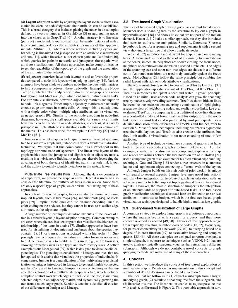
Fig. 2. From (a) a graph, to (b) a spanning tree of a subgraph. Note that node F is not included and that several edges are missing (e.g., B-D).(c) Linearization of the tree shown in (b). The linear tree layout allows us to juxtapose a table showing hidden edges and overall node degree, anadjacency matrix, and a table showing rich node attributes. Hidden links are shown for the selected node B. (d) Level layout of the same tree, whereall nodes at the same distance from the root are grouped together. (e) Node sorting to ensure that all nodes on path A-D-G are in sequence.

allows us to visualize additional topological information, such as nodeadjacency, and to show associated attributes of the nodes. Although thefirst two steps are common in other systems, as discussed in Section 3.2,Juniper is the first technique to make use of a dynamically extractedtree to visualize multivariate attributes.

Figure 2(a) shows an example graph. In practice, this graph can belarger than can be conveniently displayed, can have different types ofnodes, and can have rich attributes associated with it. Following the“search, show context, expand on demand” principle [49], we extract asubgraph from the larger graph — either in bulk or iteratively — andcalculate a spanning tree for that subgraph using a breadth-first search(Figure 2(b)). If a subgraph is added in bulk, a key decision in thisprocess is the choice of the root node, since the tree-based approachworks best for tasks related to the root (e.g., it is trivial to see allneighbors of the root). We assume that analysts will want to manuallyspecify a root in most cases; if no root is specified, we choose thenode with the highest degree. The order in which nodes are visited at agiven level by the breadth-first search algorithm also has an impact onthe resulting tree, as nodes visited first will likely have more of theirneighbors available to be attached. In Juniper, the order is driven by auser-defined sorting function; sensible options include lexical orderingof node labels, ordering by degree, or ordering by attributes.

4.1 LayoutOnce a spanning tree is calculated, we linearize the tree using oneof two complementary layout algorithms. We produce a traditionaltree layout using a depth-first search algorithm, where every node isassigned a unique vertical position (see Figure 2(c)). The order ofnodes for layout purposes is again defined with a sorting function.

An alternative layout is the level layout, shown in Figure 2(d). In thelevel layout, all nodes of a level are shown next to each other, followedby all nodes of the next level, etc. Again, sorting of nodes is driven bya user-specified function.

Level layout and tree layout have complementary strengths. Thetree layout is well suited to investigate precise relationships to the rootnode. For example, in the bipartite co-author network, if we start withan author, we can expand all her publications, and then expand all theco-authors on each of these publications, giving us a sense of whocollaborated on which paper. The level layout, in contrast, allows us toask a different question. In the level layout, the root author would beat level one, all her papers at level two, and all her co-authors at levelthree. In this layout, we can easily see and compare all the co-authorsof the root author; they will be next to each other, and we can use thetable to sort the nodes, to identify, for example, the author with themost papers. In general, the tree layout can be used to answer questionsabout specific topology, whereas the level layout can be used to evaluateall nodes at a certain distance. Note that level and tree layouts can beseparately defined for each branch.

Both level and tree layouts are well suited to support one of our main

tasks: understanding attributes in the context of neighborhoods. Tosupport our other main task — understanding attributes in the contextof paths — we introduce path-based node sorting as illustrated in Fig-ure 2(e). In this example, the tree shown in Figure 2(b) was reorderedto guarantee that all nodes along the path A-D-G are in the sequenceof the path, thereby supporting the analysis of its attribute in sequenceand enabling analysts to make judgments about path effects.

4.2 Reshaping the Tree and Revealing Hidden Edges

The crossing-free and easily readable layout achieved by using a span-ning tree comes at a cost — both tree and level layouts hide edges. Asimple way to reveal all edges and neighbors of a node is to make itthe root. This, however, changes the layout drastically, which can bedisorienting for an analyst. An alternative is to gather all children ofa node. In that case, all nodes that have an edge to the target node areattached as children to this node, with the exception of its ancestors.We choose not to attach ancestors as children because it would lead tosimilar layout changes as the make-root operation.

In addition to reshaping, we use three strategies to visualize edgesthat are not part of the tree. First, hidden edges are drawn for user-selected nodes. In Figure 2(c), hidden edges are drawn for node B,which has edges to nodes C and D, in addition to the edges to A andE that are part of the tree. This strategy is common to most tree-basedgraph visualization techniques (e.g., [32]).

Complementary to showing hidden edges on demand, we also showa table visualizing counts for hidden edges (the number of hiddenedges in the subgraph) and graph edges (the degree of the node inthe underlying graph), as shown in Figure 2(c). Whereas the formerallows analysts to judge connections that are not apparent in the tree,the latter can be used to judge the node relative to the whole network,and also give analysts a sense of how many nodes would be added ifthe neighbors of the node were to be added to the subgraph.

The third strategy to visualize topology is an adjacency matrix that isfully integrated with the tree, resulting in a hybrid node-link/matrix lay-out. The matrix is not meant to show all nodes in the subgraph, as thiswould likely result in a sparse matrix and require considerable amountsof screen-space. Instead, similar to the rationale behind NodeTrix [20],the matrix is designed to show connectivity for highly connected nodes.The integration of the node-link tree and the matrix allows analysts toquickly judge the relationships of these nodes with nodes in the tree.Note that any node can be included in the adjacency matrix, not onlythose that are part of the subgraph. Figure 2(c), for example, showsnode F in the adjacency matrix, which is not included in the subgraph.The adjacency matrix can be useful, for example, when exploring anauthor’s papers and co-authors. Adding the author’s PhD and postdocadvisors to the matrix is useful since she has likely collaborated onmany papers. Using the matrix, an analyst can quickly judge whichpapers were written in collaboration with whom, which would not beeasy to see in the tree visualization alone.

A

B

E

D

C

G

H

F

A

B

ED

C

G

H

F

(a) Aggregating a Tree Layout.

A

B

E

D

C

G

H

F

A

B EDC

G HF

(b) Aggregating a Level Layout.

A

B

EDC

G

HF

(c) Aggregating with DOI.

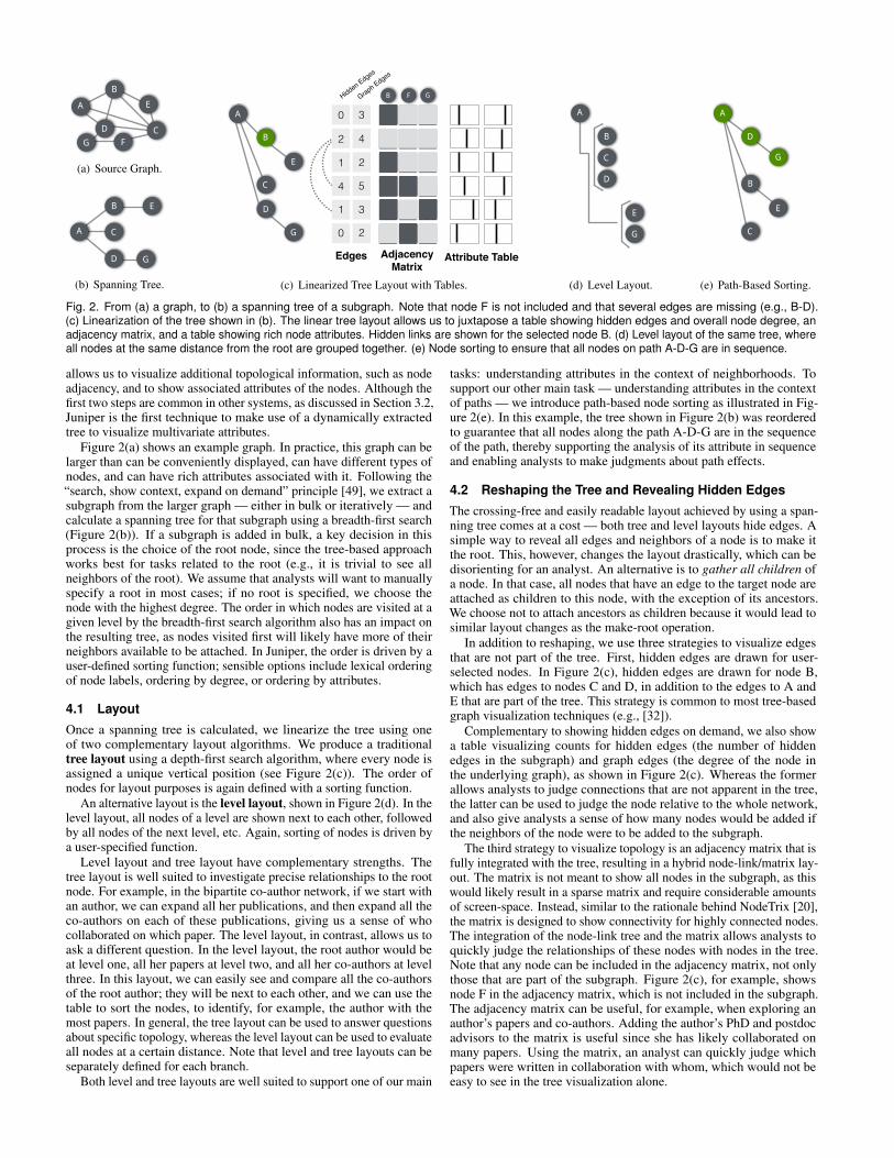
Fig. 3. Aggregation strategies. (a) Aggregation in tree layout: leaves of the same parent are aggregated by placing them in the same row. (b)Aggregating in level mode: nodes of the same level are aggregated into a single row. (c) Aggregation with a degree-of-interest function, shown in alevel mode. Nodes B and G (green) are considered to be of interest based on a degree-of-interest function, and hence are placed in their own row.

4.3 Hiding and Aggregation

Although a tree-based linear layout has many advantages, it also limitsthe number of nodes that can be concurrently displayed on the screen.To counteract this limitation, we introduce two approaches to selectivelyreduce the number of nodes: branch hiding and branch aggregation.

Branch hiding is common to most tree visualizations. It allowsanalysts to selectively hide branches of a tree that may not be relevantfor the task at hand. Although it excels at saving space, the downside ofhiding is that analysts no longer have access to any information aboutthe hidden nodes.

Our second, less aggressive, approach is aggregation. This approachhas the advantage of preserving both topological and attribute informa-tion in aggregate form. Aggregation is available in both tree and levelmodes. In tree mode, illustrated in Figure 3(a), only leaves are aggre-gated; the backbone of the tree and hence all the topological structureof the tree remain visible. When aggregating in level mode, as shownin Figure 3(b), all the nodes of one level are aggregated into a singlerow, resulting in a very compact layout.

Aggregation as described above can be controlled using the tree’stopology, i.e., analysts can choose to represent individual branches inaggregated mode. However, it is a common task to look for nodeswith certain attribute characteristics among such a large, aggregatedset. To address this, we introduce a binary degree-of-interest (DOI)function [12]. Figure 3(c) illustrates the effect of a DOI function onlevel-based aggregation. Here two nodes, B and G, shown in color,are considered of interest and hence retain their own row, whereas theothers are aggregated. An example for the co-author network wouldbe to look for all highly cited papers of a network of prolific authors,in which case highly cited papers would be afforded their own rows,whereas papers with few citations would be aggregated.

Note that the visualization of hidden edges, the adjacency matrix,and the attribute visualization can easily be adapted to support bothindividual and aggregated rows.

4.4 Attribute Visualization

In line with the “topological attributes” shown in the edge count tableand the adjacency matrix, we can leverage the linearized layout tovisualize arbitrary node attributes, as illustrated in Figure 2(c). Avariety of visualization options can conceivably show different datatypes in either individual or aggregated form [11].

The key benefit of the integrated attribute visualization, as opposedto a separate linked view, is that the topology of the tree can be used tosort and group the elements, revealing, e.g., dependencies along a path,or shared characteristics of all neighbors of a node. Equally valuableis the opposite approach: the attribute visualizations can be used toinfluence the tree layout, through both sorting and DOI functions. Thecolumns representing attributes are well suited to interactively definesuch a sorting, or a data range of interest for a DOI, as shown inFigure 4.

5 DESIGN

We implemented the concept described in the previous section in aninteractive web-based tool. Here we report on the design decisions thatwent into realizing this tool.

Juniper has two views: (1) a query view that is used to search forindividual nodes or to query for subgraphs, and (2) the main tree+tableview, which contains the graph and attribute visualizations. A toolbarat the top allows analysts to switch to a force-directed layout and tochoose a dataset. In addition, node-type specific menus allow analyststo add attributes to the table and to filter nodes by type.

5.1 QueryingThe query interface is the starting point for any exploration in Juniper.Analysts can browse or search for nodes in the query view and addthem to the tree+table view (see Figure 1). The search and browsinginterface is faceted by node types: when, for example, text is entered inthe search field, all matches are shown in separate, type-specific facets.The faceting enables analysts to quickly find nodes of interest, evenwith an incomplete query. The interface also shows the degree of thenodes, so that highly connected nodes can be readily identified. A nodecan be added individually or together with all its neighbors. Nodes canalso be added to the adjacency matrix. It is possible to add multipleroots/trees to the tree+table view simultaneously.

The query view also provides an interface to write Neo4J Cypherqueries (a query language for the graph database we use). Although thisis an expert option, it enables analysts to retrieve arbitrary subgraphsconsidering both topological features and attributes.

5.2 Tree ViewThe tree view implements the concept outlined in Section 4. Nodes ateach level are given ample space for labels, which is a common limita-tion in force-directed layouts. We also distinguish between differentnode types by showing a custom symbol for each type. Edge types anddirections are shown as tool-tips where available.

The graph can be grown organically by revealing neighboring nodes.In cases where a node has more neighbors than are currently shown, asmall plus sign is shown below the node that can be used to add thosemissing nodes, as shown in Figure 4.

In terms of tree-restructuring, our prototype supports the previouslydiscussed make root and gather children operations, in addition to se-lectively removing nodes/branches, and explicitly reattaching a branchat a different node, based on a hidden edge. Hidden edges are shownfor the selected node, House Stark, in Figure 4.

Layout and AggregationFigure 4 shows the implementation of the previously described layoutstrategies. The example shown is a Game of Thrones network that con-tains many different node types. The tree originates at a person, EddardStark, who has a connection to the û Battle at the Mummer’s Ford viaan intermediate person, Robb Stark. The layout at the root is a treelayout, but descendants of Joffrey Baratheon are shown in level layout,

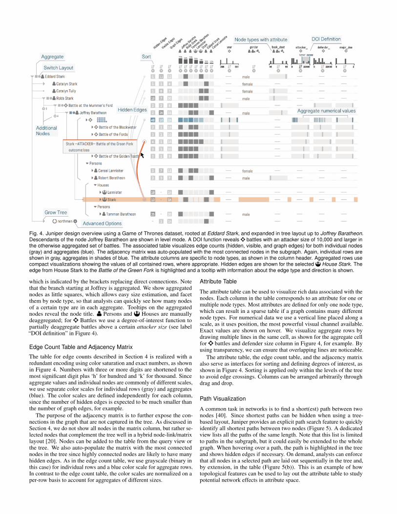
Fig. 4. Juniper design overview using a Game of Thrones dataset, rooted at Eddard Stark, and expanded in tree layout up to Joffrey Baratheon.Descendants of the node Joffrey Baratheon are shown in level mode. A DOI function reveals û battles with an attacker size of 10,000 and larger inthe otherwise aggregated set of battles. The associated table visualizes edge counts (hidden, visible, and graph edges) for both individual nodes(gray) and aggregates (blue). The adjacency matrix was auto-populated with the most connected nodes in the subgraph. Again, individual rows areshown in gray, aggregates in shades of blue. The attribute columns are specific to node types, as shown in the column header. Aggregated rows usecompact visualizations showing the values of all contained rows, where appropriate. Hidden edges are shown for the selected House Stark. Theedge from House Stark to the Battle of the Green Fork is highlighted and a tooltip with information about the edge type and direction is shown.

which is indicated by the brackets replacing direct connections. Notethat the branch starting at Joffrey is aggregated. We show aggregatednodes as little squares, which allows easy size estimation, and facetthem by node type, so that analysts can quickly see how many nodesof a certain type are in each aggregate. Tooltips on the aggregatednodes reveal the node title. g Persons and Houses are manuallydeaggregated; for û Battles we use a degree-of-interest function topartially deaggregate battles above a certain attacker size (see label“DOI definition” in Figure 4).

Edge Count Table and Adjacency Matrix

The table for edge counts described in Section 4 is realized with aredundant encoding using color saturation and exact numbers, as shownin Figure 4. Numbers with three or more digits are shortened to themost significant digit plus ‘h’ for hundred and ‘k’ for thousand. Sinceaggregate values and individual nodes are commonly of different scales,we use separate color scales for individual rows (gray) and aggregates(blue). The color scales are defined independently for each column,since the number of hidden edges is expected to be much smaller thanthe number of graph edges, for example.

The purpose of the adjacency matrix is to further expose the con-nections in the graph that are not captured in the tree. As discussed inSection 4, we do not show all nodes in the matrix column, but rather se-lected nodes that complement the tree well in a hybrid node-link/matrixlayout [20]. Nodes can be added to the table from the query view orthe tree. We also auto-populate the matrix with the most connectednodes in the tree since highly connected nodes are likely to have manyhidden edges. As in the edge count table, we use grayscale (binary inthis case) for individual rows and a blue color scale for aggregate rows.In contrast to the edge count table, the color scales are normalized on aper-row basis to account for aggregates of different sizes.

Attribute Table

The attribute table can be used to visualize rich data associated with thenodes. Each column in the table corresponds to an attribute for one ormultiple node types. Most attributes are defined for only one node type,which can result in a sparse table if a graph contains many differentnode types. For numerical data we use a vertical line placed along ascale, as it uses position, the most powerful visual channel available.Exact values are shown on hover. We visualize aggregate rows bydrawing multiple lines in the same cell, as shown for the aggregate cellfor û battles and defender size column in Figure 4, for example. Byusing transparency, we can ensure that overlapping lines are noticeable.

The attribute table, the edge count table, and the adjacency matrixalso serve as interfaces for sorting and defining degrees of interest, asshown in Figure 4. Sorting is applied only within the levels of the treeto avoid edge crossings. Columns can be arranged arbitrarily throughdrag and drop.

Path Visualization

A common task in networks is to find a short(est) path between twonodes [40]. Since shortest paths can be hidden when using a tree-based layout, Juniper provides an explicit path search feature to quicklyidentify all shortest paths between two nodes (Figure 5). A dedicatedview lists all the paths of the same length. Note that this list is limitedto paths in the subgraph, but it could easily be extended to the wholegraph. When hovering over a path, the path is highlighted in the treeand shows hidden edges if necessary. On demand, analysts can enforcethat all nodes in a selected path are laid out sequentially in the tree and,by extension, in the table (Figure 5(b)). This is an example of howtopological features can be used to lay out the attribute table to studypotential network effects in attribute space.

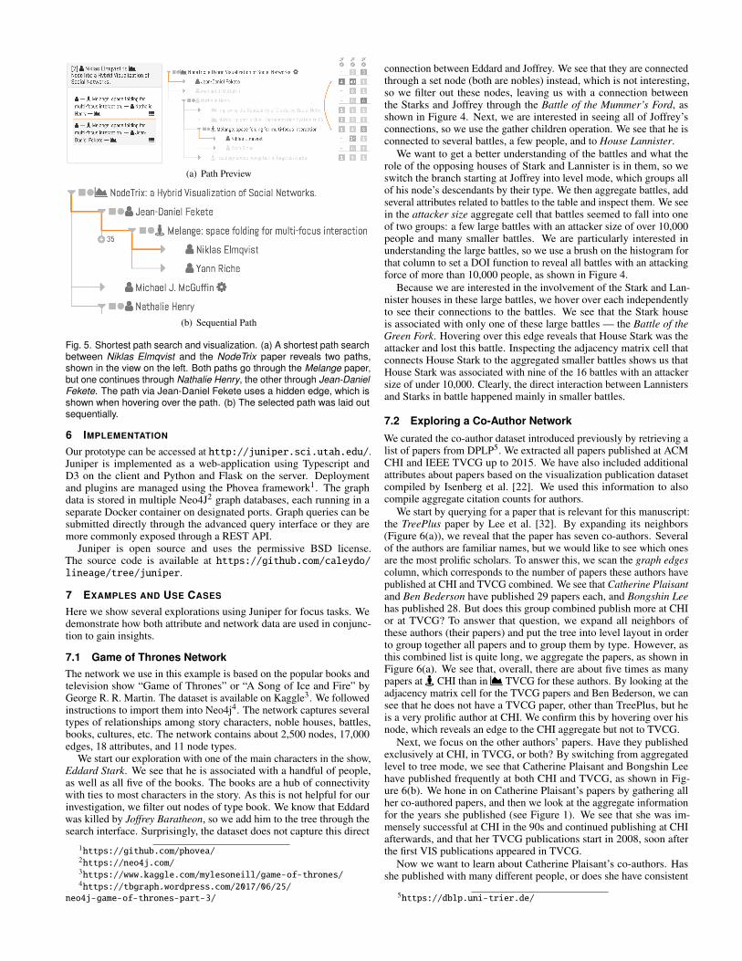
(a) Path Preview

(b) Sequential Path

Fig. 5. Shortest path search and visualization. (a) A shortest path searchbetween Niklas Elmqvist and the NodeTrix paper reveals two paths,shown in the view on the left. Both paths go through the Melange paper,but one continues through Nathalie Henry, the other through Jean-DanielFekete. The path via Jean-Daniel Fekete uses a hidden edge, which isshown when hovering over the path. (b) The selected path was laid outsequentially.

6 IMPLEMENTATION

Our prototype can be accessed at http://juniper.sci.utah.edu/.Juniper is implemented as a web-application using Typescript andD3 on the client and Python and Flask on the server. Deploymentand plugins are managed using the Phovea framework1. The graphdata is stored in multiple Neo4J2 graph databases, each running in aseparate Docker container on designated ports. Graph queries can besubmitted directly through the advanced query interface or they aremore commonly exposed through a REST API.

Juniper is open source and uses the permissive BSD license.The source code is available at https://github.com/caleydo/lineage/tree/juniper.

7 EXAMPLES AND USE CASES

Here we show several explorations using Juniper for focus tasks. Wedemonstrate how both attribute and network data are used in conjunc-tion to gain insights.

7.1 Game of Thrones NetworkThe network we use in this example is based on the popular books andtelevision show “Game of Thrones” or “A Song of Ice and Fire” byGeorge R. R. Martin. The dataset is available on Kaggle3. We followedinstructions to import them into Neo4j4. The network captures severaltypes of relationships among story characters, noble houses, battles,books, cultures, etc. The network contains about 2,500 nodes, 17,000edges, 18 attributes, and 11 node types.

We start our exploration with one of the main characters in the show,Eddard Stark. We see that he is associated with a handful of people,as well as all five of the books. The books are a hub of connectivitywith ties to most characters in the story. As this is not helpful for ourinvestigation, we filter out nodes of type book. We know that Eddardwas killed by Joffrey Baratheon, so we add him to the tree through thesearch interface. Surprisingly, the dataset does not capture this direct

1https://github.com/phovea/2https://neo4j.com/3https://www.kaggle.com/mylesoneill/game-of-thrones/4https://tbgraph.wordpress.com/2017/06/25/

neo4j-game-of-thrones-part-3/

connection between Eddard and Joffrey. We see that they are connectedthrough a set node (both are nobles) instead, which is not interesting,so we filter out these nodes, leaving us with a connection betweenthe Starks and Joffrey through the Battle of the Mummer’s Ford, asshown in Figure 4. Next, we are interested in seeing all of Joffrey’sconnections, so we use the gather children operation. We see that he isconnected to several battles, a few people, and to House Lannister.

We want to get a better understanding of the battles and what therole of the opposing houses of Stark and Lannister is in them, so weswitch the branch starting at Joffrey into level mode, which groups allof his node’s descendants by their type. We then aggregate battles, addseveral attributes related to battles to the table and inspect them. We seein the attacker size aggregate cell that battles seemed to fall into oneof two groups: a few large battles with an attacker size of over 10,000people and many smaller battles. We are particularly interested inunderstanding the large battles, so we use a brush on the histogram forthat column to set a DOI function to reveal all battles with an attackingforce of more than 10,000 people, as shown in Figure 4.

Because we are interested in the involvement of the Stark and Lan-nister houses in these large battles, we hover over each independentlyto see their connections to the battles. We see that the Stark houseis associated with only one of these large battles — the Battle of theGreen Fork. Hovering over this edge reveals that House Stark was theattacker and lost this battle. Inspecting the adjacency matrix cell thatconnects House Stark to the aggregated smaller battles shows us thatHouse Stark was associated with nine of the 16 battles with an attackersize of under 10,000. Clearly, the direct interaction between Lannistersand Starks in battle happened mainly in smaller battles.

7.2 Exploring a Co-Author Network

We curated the co-author dataset introduced previously by retrieving alist of papers from DPLP5. We extracted all papers published at ACMCHI and IEEE TVCG up to 2015. We have also included additionalattributes about papers based on the visualization publication datasetcompiled by Isenberg et al. [22]. We used this information to alsocompile aggregate citation counts for authors.

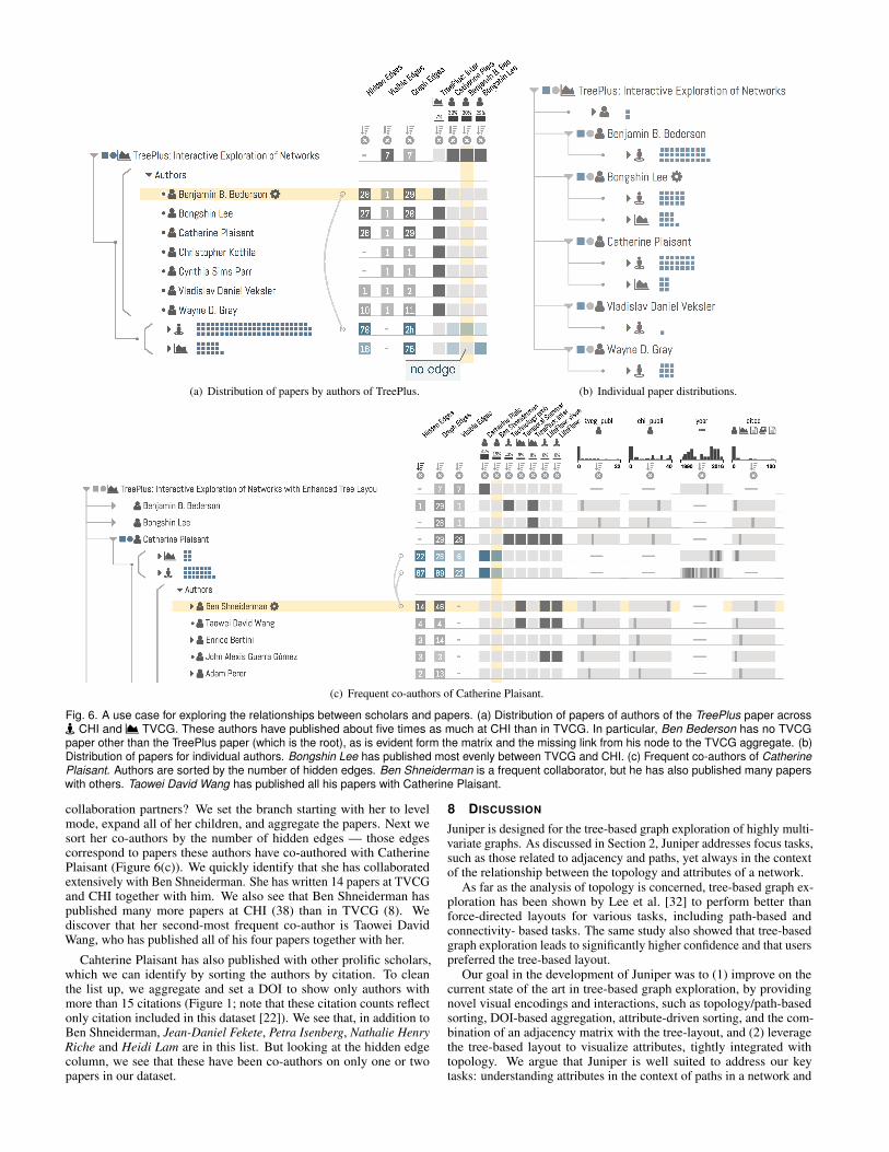
We start by querying for a paper that is relevant for this manuscript:the TreePlus paper by Lee et al. [32]. By expanding its neighbors(Figure 6(a)), we reveal that the paper has seven co-authors. Severalof the authors are familiar names, but we would like to see which onesare the most prolific scholars. To answer this, we scan the graph edgescolumn, which corresponds to the number of papers these authors havepublished at CHI and TVCG combined. We see that Catherine Plaisantand Ben Bederson have published 29 papers each, and Bongshin Leehas published 28. But does this group combined publish more at CHIor at TVCG? To answer that question, we expand all neighbors ofthese authors (their papers) and put the tree into level layout in orderto group together all papers and to group them by type. However, asthis combined list is quite long, we aggregate the papers, as shown inFigure 6(a). We see that, overall, there are about five times as manypapers at y CHI than in ^ TVCG for these authors. By looking at theadjacency matrix cell for the TVCG papers and Ben Bederson, we cansee that he does not have a TVCG paper, other than TreePlus, but heis a very prolific author at CHI. We confirm this by hovering over hisnode, which reveals an edge to the CHI aggregate but not to TVCG.

Next, we focus on the other authors’ papers. Have they publishedexclusively at CHI, in TVCG, or both? By switching from aggregatedlevel to tree mode, we see that Catherine Plaisant and Bongshin Leehave published frequently at both CHI and TVCG, as shown in Fig-ure 6(b). We hone in on Catherine Plaisant’s papers by gathering allher co-authored papers, and then we look at the aggregate informationfor the years she published (see Figure 1). We see that she was im-mensely successful at CHI in the 90s and continued publishing at CHIafterwards, and that her TVCG publications start in 2008, soon afterthe first VIS publications appeared in TVCG.

Now we want to learn about Catherine Plaisant’s co-authors. Hasshe published with many different people, or does she have consistent

5https://dblp.uni-trier.de/

(a) Distribution of papers by authors of TreePlus. (b) Individual paper distributions.

(c) Frequent co-authors of Catherine Plaisant.

Fig. 6. A use case for exploring the relationships between scholars and papers. (a) Distribution of papers of authors of the TreePlus paper acrossy CHI and ^ TVCG. These authors have published about five times as much at CHI than in TVCG. In particular, Ben Bederson has no TVCGpaper other than the TreePlus paper (which is the root), as is evident form the matrix and the missing link from his node to the TVCG aggregate. (b)Distribution of papers for individual authors. Bongshin Lee has published most evenly between TVCG and CHI. (c) Frequent co-authors of CatherinePlaisant. Authors are sorted by the number of hidden edges. Ben Shneiderman is a frequent collaborator, but he has also published many paperswith others. Taowei David Wang has published all his papers with Catherine Plaisant.

collaboration partners? We set the branch starting with her to levelmode, expand all of her children, and aggregate the papers. Next wesort her co-authors by the number of hidden edges — those edgescorrespond to papers these authors have co-authored with CatherinePlaisant (Figure 6(c)). We quickly identify that she has collaboratedextensively with Ben Shneiderman. She has written 14 papers at TVCGand CHI together with him. We also see that Ben Shneiderman haspublished many more papers at CHI (38) than in TVCG (8). Wediscover that her second-most frequent co-author is Taowei DavidWang, who has published all of his four papers together with her.

Cahterine Plaisant has also published with other prolific scholars,which we can identify by sorting the authors by citation. To cleanthe list up, we aggregate and set a DOI to show only authors withmore than 15 citations (Figure 1; note that these citation counts reflectonly citation included in this dataset [22]). We see that, in addition toBen Shneiderman, Jean-Daniel Fekete, Petra Isenberg, Nathalie HenryRiche and Heidi Lam are in this list. But looking at the hidden edgecolumn, we see that these have been co-authors on only one or twopapers in our dataset.

8 DISCUSSION

Juniper is designed for the tree-based graph exploration of highly multi-variate graphs. As discussed in Section 2, Juniper addresses focus tasks,such as those related to adjacency and paths, yet always in the contextof the relationship between the topology and attributes of a network.

As far as the analysis of topology is concerned, tree-based graph ex-ploration has been shown by Lee et al. [32] to perform better thanforce-directed layouts for various tasks, including path-based andconnectivity- based tasks. The same study also showed that tree-basedgraph exploration leads to significantly higher confidence and that userspreferred the tree-based layout.

Our goal in the development of Juniper was to (1) improve on thecurrent state of the art in tree-based graph exploration, by providingnovel visual encodings and interactions, such as topology/path-basedsorting, DOI-based aggregation, attribute-driven sorting, and the com-bination of an adjacency matrix with the tree-layout, and (2) leveragethe tree-based layout to visualize attributes, tightly integrated withtopology. We argue that Juniper is well suited to address our keytasks: understanding attributes in the context of paths in a network and

understanding attributes in the context of neighborhoods.One of the downsides of using a tree-based layout is that it is diffi-

cult to understand cycles in a network. Although we believe that thevisualization of hidden edges makes it possible to do that in Juniper,it is not the ideal solution because it requires interaction to uncover acycle. We are considering various strategies to address this problem,including a supplemental view for cycles, a special encoding along thetree, or breaking with the tree-convention for selected nodes.

Our technique targets focus tasks, yet overviews can be useful insome scenarios. Although we chose not to include an overview visual-ization to be concise and focused, we envision that a production-qualitygraph analysis system would also provide overview techniques as, forexample, described by van den Elzen and van Wijk [48]. In such an in-tegrated tool, analysts could seamlessly switch between representationsoptimized for overview and focus tasks.

8.1 ScalabilitySince Juniper is a bottom-up graph visualization technique, the size ofthe underlying graph is limited only by the capabilities and performanceof the graph database. The largest network we currently include inour demo (the co-author network) has about 34,000 nodes and 90,000edges and results in no noticeable delays for common queries.

The scalability of the subgraph is limited by the number of rows thatcan be simultaneously displayed. On a large desktop screen, we canshow about 50-60 rows. The number of rows, however, corresponds tothe number of nodes only when no aggregation is used. We found thatthe use of aggregation combined with a DOI function is a very efficientway to explore subgraphs with a few hundred nodes, depending on theproperties of the network. In cases where more rows are displayed thancan be fit on the screen, we use scrolling. However, we currently donot provide a good solution for linking to off-screen content; henceworking with many more rows can be tedious.

In terms of the number of attributes, Juniper is exceptionally scal-able compared to other multivariate network visualization techniques.We consciously reserve a sizable portion of the available screen formaking long node labels, such as paper titles, readable. Even withthat much space dedicated to labels, we can display 10-20 additionalattribute columns on a desktop display. Our current visual encodingsfor attribute visualization favor precision and details over compactness;more compact representations, such as those used in enRoute [41] areconceivable and could increase that number considerably.

8.2 Comparison to Related TechniquesWe compare Juniper to TreePlus [32], since TreePlus is the most com-prehensive of all the tree-based graph visualization techniques dis-cussed in Section 3.2. Although TreePlus shares the basic idea oftree-based graph exploration with Juniper and was an important inspi-ration for our work, Juniper introduces several novel concepts that gosignificantly beyond the capabilities of TreePlus. The key distinctionfrom TreePlus is our ability to visualize rich attribute data, dueto the linearized layout and the juxtaposition with the table. How-ever, we also argue that Juniper is at least competitive with TreePluswhen considering only topological tasks. Even though the linear layoutneeds more space than the layout chosen in TreePlus, we argue thatour aggregation methods counteract the increased spatial demand ofthe linear layout, and that our DOI-based deaggregation is effectiveat revealing relevant nodes and connections even when aggregation isused. TreePlus also does not have a level layout, which can be used toquickly identify nodes at a certain distance from the root.

Lineage [39] is a domain-specific tool developed for visualizingclinical genealogies and was published recently by some authors of thismanuscript. Although Lineage shares the idea of using a linearizedtree to visualize multivariate attributes of that tree in a table, it is infact a tree visualization tool, and not a general graph visualizationtechnique, like Juniper. The genealogies that can be visualized inLineage have to be tree-like, i.e., have to trace back to a single founder.Rare cross-links within the tree are removed by duplicating the nodes ina preprocessing step. Since Lineage visualizes trees, it has no notion ofre-shaping a tree based on a graph, does not show topological context

by combined a node link and a matrix layout, and can represent onlystatic instances of a tree, instead of growing a tree from a subgraph thatis dynamically extracted from a large graph. Lineage does not supportpath-linearization and has no level mode. Lineage is an importanttool in its niche application area. Juniper, in contrast, is a generalpurpose multivariate graph visualization technique with the potentialfor applications in many domains.

8.3 EvaluationWe considered various strategies to evaluate Juniper against the claimswe make: that it is a well-suited technique for focus tasks in multivari-ate network analysis. We considered qualitative/usability evaluation,case studies, and insight-based evaluation, which we have rejectedfor different reasons. Ultimately, we decided between (1) quantitativeevaluation of task performance (time, correctness) and (2) evaluationby justifying the design rationale and providing usage scenarios.

With regard to quantitative evaluation, the key choices to make inthe study design are (1) the tasks to use in the evaluation and (2) thecomparison target. A comparison to a state-of-the-art system like Cy-toscape introduces confounders and makes comparisons between atool specifically designed for certain tasks with a general purpose tool.The best approach to quantitatively evaluate the core contribution ofa complex technique such as Juniper would be to implement a reason-able alternative in the same general framework. We could compareJuniper to an MCV system using our attribute table and a force-directedlayout. However, while we provide a simple force-directed layout forillustration in our prototype implementation, we do not provide ad-vanced features such as aggregation, expanding or collapsing branches,etc. Since we have no canonical way to implement these features, thisapproach would require significant effort in designing such a system.It would also introduce additional potential confounders, because itmatters how (well) these features are implemented.

We instead opt for evaluation by providing a detailed rationale forour design [16] and demonstrate its usefulness in use cases. In line withrecent successful papers (e.g. [21, 34, 47, 48]), we believe that designarguments and demonstrations through use cases provide excellentevidence for the utility of complex, interactive visualization techniques.

9 CONCLUSION AND FUTURE WORK

We believe that Juniper is widely applicable to different graph datasetsacross various domains. Juniper’s strengths are in interactive explo-ration and in supporting focus tasks for multivariate graph visualization.In the future we hope to develop techniques for connecting to off-screennodes, which is a current scalability limitation. Also, allowing duplicatenodes could be helpful for certain tasks, yet node duplication requirescareful encoding to not confuse users. Juniper currently also does notsupport rich edge attributes. Edge attributes of visible edges could beseamlessly integrated into Juniper, as the tree structure guarantees thateach node has exactly one incoming edge. As a result, we could addrows representing edges to the table right above the destination nodeand add columns for the edge attributes. A drawback to this solution isthat it cannot be used for hidden edges. Attributes of multiple hiddenedges could be shown as extra columns in the table with their destina-tion node, visualizing attributes from multiple edge in each cell. Finally,for graphs with many different node types, the attribute table can besparse. We plan to investigate interleaving cells for different attributesin a single column to remedy this.

ACKNOWLEDGMENTS

The authors wish to thank members of the Visualization Design Labfor their feedback, and acknowledge support by NIH (U01 CA198935),NSF (IIS 1751238), DoD (ST1605-16-01), and the Austrian ScienceFund (FWF P27975-NBL).

REFERENCES

[1] A. Barsky, T. Munzner, J. Gardy, and R. Kincaid. Cerebral: VisualizingMultiple Experimental Conditions on a Graph with Biological Context.IEEE Transactions on Visualization and Computer Graphics (InfoVis ’08),14(6):1253–1260, 2008. doi: 10.1109/TVCG.2008.117

[2] M. Bastian, S. Heymann, and M. Jacomy. Gephi: An Open SourceSoftware for Exploring and Manipulating Networks. In Third InternationalAAAI Conference on Weblogs and Social Media, Mar. 2009.

[3] A. Bezerianos, F. Chevalier, P. Dragicevic, N. Elmqvist, and J. D. Fekete.GraphDice: A System for Exploring Multivariate Social Networks. Com-puter Graphics Forum (EuroVis ’10), 29(3):863–872, 2010. doi: 10.1111/j.1467-8659.2009.01687.x

[4] M. Burch, F. Beck, and S. Diehl. Timeline Trees: Visualizing Sequencesof Transactions in Information Hierarchies. In Proceedings of the WorkingConference on Advanced Visual Interfaces, AVI ’08, pp. 75–82. ACM,New York, NY, USA, 2008. doi: 10.1145/1385569.1385584

[5] N. A. Christakis and J. H. Fowler. The Spread of Obesity in a Large SocialNetwork over 32 Years. New England Journal of Medicine, 357(4):370–379, July 2007. doi: 10.1056/NEJMsa066082

[6] C. Dunne, N. Henry Riche, B. Lee, R. Metoyer, and G. Robertson. Graph-Trail: Analyzing Large Multivariate, Heterogeneous Networks WhileSupporting Exploration History. In Proceedings of the ACM SIGCHIConference on Human Factors in Computing Systems (CHI ’12), pp. 1663–1672. ACM, 2012. doi: 10.1145/2207676.2208293

[7] M. B. Eisen, P. T. Spellman, P. O. Brown, and D. Botstein. Clusteranalysis and display of genome-wide expression patterns. Proceedings ofthe National Academy of Sciences USA, 95(25):14863–14868, 1998. doi:10.1073/pnas.95.25.14863

[8] P. Eklund, N. Roberts, and S. Green. OntoRama: Browsing RDF ontolo-gies using a hyperbolic-style browser. In First International Symposium onCyber Worlds, 2002. Proceedings., pp. 405–411, 2002. doi: 10.1109/CW.2002.1180907

[9] N. Elmqvist, T.-N. Do, H. Goodell, N. Henry, and J. Fekete. ZAME:Interactive Large-Scale Graph Visualization. In Visualization Symposium,2008. PacificVIS ’08. IEEE Pacific, pp. 215–222, 2008. doi: 10.1109/PACIFICVIS.2008.4475479

[10] J.-D. Fekete, D. Wang, N. Dang, A. Aris, and C. Plaisant. InteractivePoster: Overlaying Graph Links on Treemaps. In Proceedings of the IEEESymposium on Information Visualization (InfoVis ’03), pp. 82–83. IEEE,2003.

[11] K. Furmanova, S. Gratzl, H. Stitz, T. Zichner, M. Jaresova, M. Ennemoser,A. Lex, and M. Streit. Taggle: Scalable Visualization of Tabular Datathrough Aggregation. arXiv preprint, 2018.

[12] G. W. Furnas. Generalized fisheye views. In Proceedings of the SIGCHIConference on Human Factors in Computing Systems (CHI ’86), pp. 16–23.ACM, 1986. doi: 10.1145/22339.22342

[13] N. Gehlenborg, S. I. O’Donoghue, N. S. Baliga, A. Goesmann, M. A.Hibbs, H. Kitano, O. Kohlbacher, H. Neuweger, R. Schneider, D. Tenen-baum, and A.-C. Gavin. Visualization of omics data for systems biology.Nature Methods, 7(3):56–68, 2010. doi: 10.1038/nmeth.1436

[14] M. Ghoniem, J.-D. Fekete, and P. Castagliola. On the Readability ofGraphs Using Node-Link and Matrix-Based Representations: A Con-trolled Experiment and Statistical Analysis. Information Visualization,4(2):114 –135, June 2005. doi: 10.1057/palgrave.ivs.9500092

[15] L. Gou and X. Zhang. Treenetviz: Revealing patterns of networks over treestructures. IEEE Transactions on Visualization and Computer Graphics(InfoVis ’11), 17(12):2449–2458, 2011.

[16] S. Greenberg and B. Buxton. Usability Evaluation Considered Harmful(Some of the Time). In Proceedings of the SIGCHI Conference on HumanFactors in Computing Systems, CHI ’08, pp. 111–120. ACM, New York,NY, USA, 2008. doi: 10.1145/1357054.1357074

[17] M. C. Hao, M. Hsu, U. Dayal, and A. Krug. Web-Based Visualization ofLarge Hierarchical Graphs Using Invisible Links in a Hyperbolic Space.In Advances in Visual Information Management, IFIP — The InternationalFederation for Information Processing, pp. 83–94. Springer, Boston, MA,2000. doi: 10.1007/978-0-387-35504-7 6

[18] J. Heer and D. Boyd. Vizster: Visualizing online social networks. In IEEESymposium on Information Visualization, 2005. INFOVIS 2005, pp. 32–39,Oct. 2005. doi: 10.1109/INFVIS.2005.1532126

[19] N. Henry and J.-D. Fekete. MatLink: Enhanced Matrix Visualization forAnalyzing Social Networks. In C. Baranauskas, P. Palanque, J. Abascal,and S. D. J. Barbosa, eds., Human-Computer Interaction – INTERACT2007, number 4663 in Lecture Notes in Computer Science, pp. 288–302.Springer Berlin Heidelberg, 2007.

[20] N. Henry, J. D. Fekete, and M. J. McGuffin. NodeTrix: A Hybrid Visu-alization of Social Networks. IEEE Transactions on Visualization andComputer Graphics (InfoVis ’07), 13(6):1302–1309, 2007. doi: 10.1109/TVCG.2007.70582

[21] D. Holten. Hierarchical Edge Bundles: Visualization of Adjacency Re-lations in Hierarchical Data. IEEE Transactions on Visualization andComputer Graphics (InfoVis ’06), 12(5):741–748, 2006. doi: 10.1109/TVCG.2006.147

[22] P. Isenberg, F. Heimerl, S. Koch, T. Isenberg, P. Xu, C. D. Stolper, M. Sedl-mair, J. Chen, T. Moller, and J. Stasko. Vispubdata.org: A MetadataCollection About IEEE Visualization (VIS) Publications. IEEE Transac-tions on Visualization and Computer Graphics, 23(9):2199–2206, Sept.2017. doi: 10.1109/TVCG.2016.2615308

[23] T. J. Jankun-Kelly and K.-L. Ma. MoireGraphs: Radial focus+contextvisualization and interaction for graphs with visual nodes. In IEEE Sym-posium on Information Visualization 2003 (IEEE Cat. No.03TH8714), pp.59–66, Oct. 2003. doi: 10.1109/INFVIS.2003.1249009

[24] B. Johnson and B. Shneiderman. Tree-maps: A space-filling approach tothe visualization of hierarchical information structures. In Proceedings ofthe IEEE Conference on Visualization (Vis ’91), pp. 284–291, 1991. doi:10.1109/VISUAL.1991.175815

[25] S. Kairam, N. H. Riche, S. Drucker, R. Fernandez, and J. Heer. Refinery:Visual Exploration of Large, Heterogeneous Networks Through Associa-tive Browsing. Computer Graphics Forum (EuroVis ’15), 34:301–310,2015.

[26] A. Kerren, H. C. Purchase, and M. Ward, eds. Multivariate NetworkVisualization. Number 8380 in Lecture notes in computer science. Springer,2014.

[27] E. Kerzner, A. Lex, C. L. Sigulinsky, R. E. Marc, B. W. Jones, T. Urness,and M. Meyer. Graffinity: Visualizing Connectivity in Large Graphs.Computer Graphics Forum (EuroVis ’17), 36(3):251–260, 2017.

[28] L. Kreft, A. Botzki, F. Coppens, K. Vandepoele, and M. Van Bel. PhyD3: Aphylogenetic tree viewer with extended phyloXML support for functionalgenomics data visualization. Bioinformatics, 33(18):2946–2947, Sept.2017. doi: 10.1093/bioinformatics/btx324

[29] J. B. Kruskal and J. M. Landwehr. Icicle Plots: Better Displays forHierarchical Clustering. The American Statistician, 37(2):162, 1983. doi:10.2307/2685881

[30] B. Lee, K. Brown, Y. Hathout, and J. Seo. GOTreePlus: An interactivegene ontology browser. Bioinformatics, 24(7):1026–1028, Apr. 2008. doi:10.1093/bioinformatics/btn068

[31] B. Lee, L. Nachmanson, G. Robertson, J. M. Carlson, and D. Heckerman.PhyloDet: A scalable visualization tool for mapping multiple traits tolarge evolutionary trees. Bioinformatics, 25(19):2611–2612, 2009. doi: 10.1093/bioinformatics/btp454

[32] B. Lee, C. S. Parr, C. Plaisant, B. B. Bederson, V. D. Veksler, W. D.Gray, and C. Kotfila. TreePlus: Interactive Exploration of Networkswith Enhanced Tree Layouts. IEEE Transactions on Visualization andComputer Graphics, 12(6):1414–1426, Nov. 2006. doi: 10.1109/TVCG.2006.106

[33] B. Lee, C. Plaisant, C. S. Parr, J.-D. Fekete, and N. Henry. Task Taxonomyfor Graph Visualization. In Proceedings of the AVI Workshop on BEyondTime and Errors: Novel Evaluation Methods for Information Visualization(BELIV ’06), pp. 1–5, 2006. doi: 10.1145/1168149.1168168

[34] A. Lex, N. Gehlenborg, H. Strobelt, R. Vuillemot, and H. Pfister. UpSet:Visualization of Intersecting Sets. IEEE Transactions on Visualizationand Computer Graphics (InfoVis ’14), 20(12):1983–1992, 2014. doi: 10.1109/TVCG.2014.2346248

[35] A. Lex, M. Streit, E. Kruijff, and D. Schmalstieg. Caleydo: Design andEvaluation of a Visual Analysis Framework for Gene Expression Datain its Biological Context. In Proceedings of the IEEE Symposium onPacific Visualization (PacificVis ’10), pp. 57–64. IEEE, 2010. doi: 10.1109/PACIFICVIS.2010.5429609

[36] A. Lex, M. Streit, H.-J. Schulz, C. Partl, D. Schmalstieg, P. J. Park, andN. Gehlenborg. StratomeX: Visual Analysis of Large-Scale HeterogeneousGenomics Data for Cancer Subtype Characterization. Computer GraphicsForum (EuroVis ’12), 31(3):1175–1184, 2012. doi: 10.1111/j.1467-8659.2012.03110.x

[37] M. Meyer, B. Wong, M. Styczynski, T. Munzner, and H. Pfister. Pathline:A Tool For Comparative Functional Genomics. Computer Graphics Forum(EuroVis ’10), 29(3):1043–1052, 2010. doi: 10.1111/j.1467-8659.2009.01710.x

[38] T. Munzner. Drawing Large Graphs with H3Viewer and Site Manager.In Graph Drawing, Lecture Notes in Computer Science, pp. 384–393.Springer, Berlin, Heidelberg, Aug. 1998. doi: 10.1007/3-540-37623-2 30

[39] C. Nobre, N. Gehlenborg, H. Coon, and A. Lex. Lineage: VisualizingMultivariate Clinical Data in Genealogy Graphs. Transaction on Visual-

ization and Computer Graphics, PP, 2018. to appear. doi: 10.1109/TVCG.2018.2811488

[40] C. Partl, S. Gratzl, M. Streit, A. M. Wassermann, H. Pfister, D. Schmalstieg,and A. Lex. Pathfinder: Visual Analysis of Paths in Graphs. ComputerGraphics Forum (EuroVis ’16), 35(3):71–80, 2016. doi: 10.1111/cgf.12883

[41] C. Partl, A. Lex, M. Streit, D. Kalkofen, K. Kashofer, and D. Schmalstieg.enRoute: Dynamic Path Extraction from Biological Pathway Maps forIn-Depth Experimental Data Analysis. In Proceedings of the IEEE Sym-posium on Biological Data Visualization (BioVis ’12), pp. 107–114, 2012.doi: 10.1109/BioVis.2012.6378600

[42] R. Pienta, F. Hohman, A. Endert, A. Tamersoy, K. Roundy, C. Gates,S. Navathe, and D. H. Chau. VIGOR: Interactive Visual Exploration ofGraph Query Results. IEEE Transactions on Visualization and ComputerGraphics, 24(1):215–225, Jan. 2018. doi: 10.1109/TVCG.2017.2744898

[43] R. Shannon, T. Holland, and A. Quigley. Multivariate Graph Drawingusing Parallel Coordinate Visualisations. Technical report, University ofSt Andrews, 2008.

[44] M. E. Smoot, K. Ono, J. Ruscheinski, P.-L. Wang, and T. Ideker. Cy-toscape 2.8: New features for data integration and network visualization.Bioinformatics, 27(3):431–432, Jan. 2011. doi: 10.1093/bioinformatics/btq675

[45] J. Stasko and E. Zhang. Focus+Context Display and Navigation Tech-niques for Enhancing Radial, Space-Filling Hierarchy Visualizations. InProceedings of the IEEE Symposium on Information Vizualization (InfoVis’00), pp. 57–65. IEEE Computer Society Press, 2000. doi: 10.1109/INFVIS.2000.885091

[46] Y. Tu and H. W. Shen. GraphCharter: Combining browsing with queryto explore large semantic graphs. In 2013 IEEE Pacific VisualizationSymposium (PacificVis), pp. 49–56, Feb. 2013. doi: 10.1109/PacificVis.2013.6596127

[47] S. van den Elzen, D. Holten, J. Blaas, and J. van Wijk. Reducing Snapshotsto Points: A Visual Analytics Approach to Dynamic Network Exploration.IEEE Transactions on Visualization and Computer Graphics, 22(1):1–10,Jan. 2016. doi: 10.1109/TVCG.2015.2468078

[48] S. van den Elzen and J. van Wijk. Multivariate Network Exploration andPresentation: From Detail to Overview via Selections and Aggregations.IEEE Transactions on Visualization and Computer Graphics (InfoVis ’14),20(12):2310–2319, 2014. doi: 10.1109/TVCG.2014.2346441

[49] F. van Ham and A. Perer. Search, Show Context, Expand on Demand:Supporting Large Graph Exploration with Degree-of-Interest. IEEE Trans-actions on Visualization and Computer Graphics (InfoVis ’09), 15(6):953–960, 2009. doi: 10.1109/TVCG.2009.108

[50] T. von Landesberger, A. Kuijper, T. Schreck, J. Kohlhammer, J. van Wijk,J.-D. Fekete, and D. Fellner. Visual Analysis of Large Graphs: State-of-the-Art and Future Research Challenges. Computer Graphics Forum,30(6):1719–1749, 2011. doi: 10.1111/j.1467-8659.2011.01898.x

[51] Y. Yang, T. Dwyer, S. Goodwin, and K. Marriott. Many-to-ManyGeographically-Embedded Flow Visualisation: An Evaluation. IEEETransactions on Visualization and Computer Graphics, 23(1):411–420,Jan. 2017. doi: 10.1109/TVCG.2016.2598885

[52] K.-P. Yee, D. Fisher, R. Dhamija, and M. Hearst. Animated exploration ofdynamic graphs with radial layout. In IEEE Symposium on InformationVisualization, 2001. INFOVIS 2001., pp. 43–50, 2001. doi: 10.1109/INFVIS.2001.963279