NASATechnical NASa-T>2r40 19870015898

Paper2740

July 1987

Advanced Detection,Isolation, andAccommodation ofSensor FailuresReal-Time Evaluation

Walter C. Merrill,John C. DeLaat, andWilliam M. Bruton

LISRAi{YCOPY

.LANGLEYRESEARCHCEN./IERLIBRARY,NASA

HAM.P.TO_N,VIRGIhlIA'

https://ntrs.nasa.gov/search.jsp?R=19870015898 2018-07-08T22:18:53+00:00Z

NASATechnicalPaper2740

1987

Advanced Detection,Isolation, andAccommodation ofSensor Failures_Real-Time Evaluation

Walter C. Merrill,John C. DeLaat, andWilliam M. Bruton

Lewis Research CenterCleveland,Ohio

National Aeronauticsand SpaceAdministration

Scientific and TechnicalInformationOffice

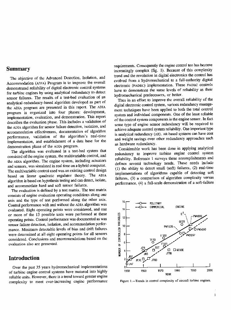
Summary requirements. Conseztuentlythe engine control toohas becomeincreasingly complex (fig. 1). Because of this complexity

The objective of the Advanced Detection, Isolation, and trend and the revolution in digital electronics the control hasAccommodation (ADIA)Program is to improve the overall evolved from a hydromechanical to a fuU-authority digital

electronic (FADEC) implementation. These FADECcontrolsdemonstrated reliability of digital electronic control systemsfor turbine engines by using analytical redundancy to detect have to demonstrate the same levels of reliability as theirsensor failures. The results of a test-bed evaluation of an hydromechanical predecessors, or better.

analytical-redundancy-based algorithm developed as part of Thus in an effort to improve the overall reliability of thethe ADIA program are presented in this report. The ADIA digital electrorticcontrol system, various re_tundancymanage-program is organized into four phases: development, ment techniques have been applied to bo_ the total controlimplementation, evaluation, and demonstration. This report system and individual components. One of the least reliabledescribes the evaluation phase. This includes a validation of of the control systemcomponents is the engine sensor. In factthe ADIAalgorithm for sensor failure detection, isolation, and some type of engine sensor redundancy will be required toaccommodation effectiveness, documentation of algorithm achieveadequate control systemreliabilit7. One importantUpeperformance, validation of the algorithm's real-time is analyticalr_undancy (AR).AR-basedsystemscan have costimplementation, and establishment of a data base for the and weight savings over other redundancy approaches such

as hardware redundancy.demonstration phase of the ADIA program.The algorithm was evaluated in a test-bed system that Considerable work has been done in applying analytical

consisted oftheenginesystem, the multivariablecontrol, and redundancy to improve turbine engine control systemthe ADIA algorithm. The engine system, including actuators reliability. Reference 1 surveys these accomplishments andand sensors, was simulated in real time on a hybrid computer, defines several technology needs. These needs includeThe multivariable control used was an existing control design (1) the ability to detect small (soft) failures, (2) real-timebased on linear quadratic regulator theory. The ADIA implementations of algorithms capable of detecting softalgorithm is bash on hypothesis testing and can detect, isolate, failures, (3) a comparison of algorithm complexity versusand accommodate hard and soft sensor failures, performance, (4) a full-scale demonstration of a soft-failure

The evaluation is defined by a test matrix. The test matrixconsists of engine evaluation operating conditions along oneaxis and the type of test performed along the other axis. 16-Control performance with and without the ADIAalgoritlunwas ---O--- MILITARY

.-r-I--- COMMERCIAL ENGINEevaluated. Eight operating points were considered, and one 14--or more of the 13 possible tests were performed at these _ E3-_operating points. Control performance was documenteAas was _ 12-- _ row4000Jsensor failure detection, isolation, and accorrmaodationperfor- _ GE23\ J_"_s"'""

> 10- PW1128--_,,,0,,'_ _.I'"mance. Minimum detectable levels of bias and drift failures _ _ ,,t,r,'O PWS000

were determined at all eight operating points for all sensors _ 8 -- _?s_'PW2O3Z_jfconsidered. Conclusions and recommendations based on the _ 6 -- f

evaluation also are presented. _ J_9,._,"I_ SST _:k#r'l .......- -9z¢[]-;/-[]O0 SEEIntroduction -= Jsz/J Jss_.__,,- Jrg0

2 JrsoOver the past 35 years hydromechanical implementations °I) J47 I I I I I

of turbine engine control systems have matured into highly 1950 1960 1970 1980 1990 2000reliable units. However, there is a trend towardgreater engine YEARcomplexity to meet ever-increasing engine performance Figure 1.--Trends in control complexity of aircraft turbine engines.

detection capability, and (5) an evaluation of the pseudo- algorithm and the implementation hardware are described.linearized modeling approach. The ADIAprogram addresses Next the results of the evaluation are presented. Finallyall of these technology needs, conclusions and recommendations for further work are given.

The ADIA program is organized into four phases:development, implementation, evaluation, and demonstration.

In the development phase (refs. 2 and 3) the ADIAalgorithm Test-Bed Systemwas designed by using advanced filtering and detection

methodologies. In the implementation phase (refs. 4 and 5) The ADIAalgorithm was evaluated in a test-bed systemthis advancedalgorithm was implemented in microprocessor- (fig. 2) consisting of the engine system, the multivariablebased hardware. A parallel-computer architecture (three control algorithm, and the ADIA algorithm. The ADIAprocessors) was used to allow the algorithm to execute in a algorithm is described in the next main section.timeframe consistent with stable, real-time operation. This

report describes the evaluation phase. In this phase algorithm Engine Systemperformance was evaluated by using a real-time hybridcomputer engine simulation. The objectives of the evaluation The engine system consisted of an F100 turbofan engine,were to validate the algorithm for sensor failure detection, the control actuators, and the sensors. The F100 turbofanisolation, and accommodation (DIA) effectiveness, to engine is a high-performance, low-bypass-ratio, twin-spooldocument algorithm performance, to validate the algorithm's turbofanengine. The test-bedengine has five controlledinputs,real-time implementation, and to establish a data base for the five sensed outputs, and four sensed environmental variables.demonstration phase of the ADIA program. The ADIA These variables are defined as follows:algorithm will be demonstrated on a full-scale F100 engine Controlled engine inputs Ucomand Umin the NASA Lewis Research Center altitude test facility. WF main combustor fuel flow

The report begins with a description of the test-bed system AJ exhaust nozzle areaused in evaluating the ADIA algorithm. Then the ADIA CIVV fan inlet variable vanes

[ FIO0TEST-REDENGINESYSTEM(HYBRIDSIMULATION) "I

I I

' . i°°i>m SENSORSII It I

I

ADIAALGORITHM , __SOFTDETECTION/

I{ ISOLATIONLOGIC

CONTROL JJ II

i,,i Ii 1ACCOMMODATIONFILTER _ I

INTEGRAL I I _1

PROTECTION

II iiI 1L JjJ zm

-.,,F------SIGNALPATH

_ RECONFIGURATIONINFORMATION

Figure 2.--Test-bed system.

Us --- FEEDFORWARDI

II --- PROPORTIONAL _-I I

PT2 , REFERENCE ENGINE

POINTSCHEDULES _ LQR PROTECTIONTT25 AND TRANSITION GAINS LOGICPLA CONTROL Z

I CRI------PT2GAIN I_TT 2

ENGINE[STATES,X SCHEDULES I___N2 s

ENGINEOUTPUTS,Z 1 INTEGRAL

i GAINS LIMITS

FTIT --_ INTEGRALTRIM

ESTIMATOR

Figure 3.--St_cture of FI_ multivariable control.

RCVV rear compressor variable vanes is more completely described in reference 6. The controlBLEED compressor bleed modes in this logic normally use fuel to set engine fan speed

Sensed engine outputs Zm and use nozzle area to set nozzle pressure (engine pressureN1 fan speed ratio). However, at those conditionswhere limiting is required,N2 compressor speed fuel flow can be used to limit the maximum FT1T,thePT4 combustor pressure maximum FT4, or the minimum PT4.PT6 exhaust nozzle pressureFTIT fan turbine inlet temperature

Sensed environmental variables Em AlgorithmPO ambient (static) pressure

PT2 fan inlet (total) pressure The ADIA algorithm detects, isolates, and accommodatesTT2 fan inlet temperature sensor failures in turbofan engine control systems. It wasTT25 compressor inlet temperature originally developed for NASA Lewis under contracts

Strictly speaking, TT25is an engine output variable. However, NAS3-22481 and NAS3-23282 by Pratt & Whitney Aircraftsince TT25 is used only as a scheduling variable in the control with subcontractor Systems Control Technology (refs. 2 and(like TT2), it is called an environmental variable. Also, TT25 3). The algorithmincorporatesadvanced falteringand detectionsensor failures are not covered by the ADIA logic, logic and is general enough to be applied to different engines

Multivariable Control System or to other types of control systems.The ADIA algorithm consists of three elements: (1) hard-The multivariable control (MVC) system (fig. 3) is failure detection and isolation logic, (2) soft-failure detection

essentially a model following proportional plus integral and isolation logic, and (3) an accommodation filter. Thesecontrol. The components of the control are the reference point are shown as part of the test-bed system in figure 2. Theschedules, the transition control schedules, the proportional algorithm detects two classesof sensor failures, hard and soft.control logic, the integral control logic, and the engine Hard failures are out-of-range or large bias errors that occurprotection logic. The reference point schedules generate a instantaneously in the sensed values. Soft failures are smalldesired engine operating point given the pilot's commanded bias errors or drift errors that accumulate relatively slowlypower lever angle (PLA). The transition logic generates rate- with time.limited command trajectories for smooth transition between The general concept is shown is block diagram form insteady-state operating points. The proportional and integral figure 4. Here, in a normal or unfailed mode of operation thecontrol logic minimizes transient and steady-state deviations accommodationfilter uses the full set of engine measurementsfrom the commandedtrajectories. The engine protection logic to generate a set of optimal estimates of the measurements.limits the size of the commanded engine inputs. This control These estimates Z are used by the control law. When a sensor

DIGITALELECTRONICCONTROLPOWERILEVER_

--_ MODEOTHERINPUTS

____ DETECTIONAND

ISOLATIONLOGIC - )

I CCOMMODATION

SIGNALS

ESTIMATOR 1IIIJ

ESTIMATEDSENSOROUTPUTS

Figure 4.--Advanced detection, isolation, and accommodation concept.

failure occurs, the detection logic determines that a failure has of the engine. The model used has a linear state-spaceoccurred. The isolation logic then determines which sensor structure, and the basepoints are nonlinear functionsof variousis faulty. This structural informationis passed to the estimator, engine variables.The estimator then removes the faulty measurement from

further consideration. The estimator, however, continues to X = F(X - Xb) + G(U - Uo)generate the full set of optimal estimates for the control. Thus

the control mode does not have to restructure for any sensor Z = H(X - Xo) + D(U - Uo) + Zofailure.

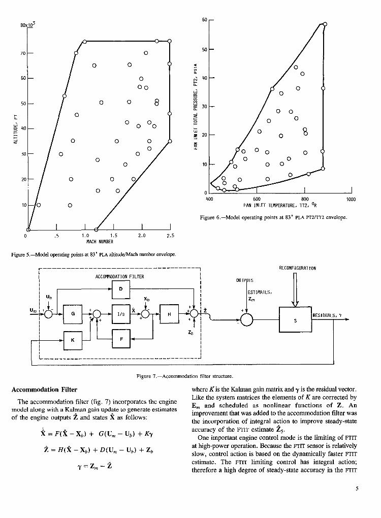
The ADIAalgorithm inputs are the measured engine inputs Here the subscriptrepresents the basepoint (steady-statepoint)Um(t ) (fuel flow, nozzle area, compressor inlet guide vane and X is the 4 × 1 model state vector, U the 5 × 1 controlangle, rear compressor variable vane angle, and bleed flow) vector, and Z the 5 × 1 output vector. The F, G, H, and Dand the measured engine outputs Zm (t) (fan speed, matrices are the appropriately dimensioned system matrices.compressor speed, combustor pressure, augmentor pressure,and fanturbineinlettemperature). The algorithmoutputsZ(t) The system matrices and the model base points wereare optimalestimatesof the engine outputs Z (t). The measured determined at 109 operating points throughout the flightenvironmental variables Emare also used to schedule engine envelope. Three variables are sufficient to completely definemodel parameters. The outputs of the algorithm, the estimates an operating point--power lever angle (PLA),altitude, andZ(t), are used as input to the proportional (linear quadratic Mach number. An alternative definition set is PEA, inletregulator, or LQR) part of the control. During normal-mode pressure (PT2),and inlet temperature (TT2).Figure 5 showssome of those 109 points as a function of the altitude/Machoperationengine measurementsare used in the integral control, number envelope at 83 ° PLA. In figure 6 the same points areWhen a sensor failure is accommodated, the measurement in shownat 83* PLAas a function of engine inlet conditions. Thethe integral control is replaced with the corresponding second envelope is the more appropriate format for ensuringaccommodation filter estimate by reconfiguring the interface that all significant model dynamics are considered byswitch matrix, adequately spanning the entire envelope with model points.

Engine Model Oncesystemmatricesare determinedat allof the 109operatingpoints, the individual matrix elements are corrected by the

The performance of the accommodation filter and the engine inlet condition E m and scheduled as nonlineardetection and isolation logic is strongly dependent on a model functions of Z. These functions are given in reference 2.

6080x103

5070 0

o oo

60 0 _ 40

O0 0o5o o o 8

_. g0

o ,_ o o,_ 0 0 O0 _- 0 0_-_40 _ 0__ _ 20 0_d 0 o o

o30 0 0 0 0 0 0

0 0 00 lO 0 0

02o 0 0 0 0

o o 0 I I400 600 800 1000

10 O FAN INLET TEMPERATURE,TT2, OR

Figure 6.--Model operating points at 83* PLAPT2/TT2envelope.

I I I I0 .5 1.0 1.5 2.0 2.5

MACHNUMBER

Figure 5.--Model operatingpointsat 83° PLAaltitude/Machnumberenvelope.

[ RECONFIGURATION

!ii ACCOMMODATIONFILTER_IF_ OUTFITSIESTIMATES"

[Figure 7.--Accommodation filter structure.

Accommodation Filter where K is the Kalman gainmatrix and 3,is the residual vector.Like the system matrices the elements of K are corrected by

The accommodation filter (fig. 7) incorporates the engine E m and scheduled as nonlinear functions of Z. Anmodel along with a Kalman gain update to generate estimates improvement that was added to theaccommodation filter wasof the engine outputs Z and states X as follows: the incorporation of integral action to improve steady-state

accuracy of the FTITestimate Zs.F(X - Xb) + G(Um - Ub) + K'y One important engine control mode is the limiting of FTIT

X

= H(X - X9) + D(Um -- Ub) + Zb at high-power operation. Because the FTIT sensor is relativelyslow, control action is based on the dynamically faster FTIT

"Y= Zm_ _ estimate. The FTIT limiting control has integral action;therefore a high degree of steady-state accuracy in the FTIT

estimate is required to ensure satisfactory control. This When a sensor failure has been isolated, the filter isaccuracy is accomplished by augmenting the filter with the reconfiguredby settingthe appropriate diagonalmatrix elementfollowing additional state and output equations: to zero. For example, if a compressor speed sensor failure

(NZ)has been isolated, the switch matrix becomes/_= K63,

1O000FTIT = Z5 + b

00000

where K6 is a gain matrix, b is the temperature bias, Z5 is S = 00100the unbiased temperature estimate, and 3, is the vector ofresiduals from the accommodationfilter. The additionof these 00010dynamics, although improving FTIT estimation accuracy,results in a larger minimum detectable FTITdrift failure rate. 00001Concatenating the temperature bias state to the filter statevector yields the same filter equations with the following The effect of this reconfiguration is to force 3'2equal to 0.

This is equivalent to setting sensed N2equal to the estimatereplacements: of N2generated by the filter. The residuals generated by the

accommodation filter are used in the hard-failure detection

Hard-Failure Detection and Isolation Logic

[ F I [ G] The hard-failure detection and isolation logic (fig. 8)0] G *-* compares the absolute'valueof each component of the residual

F *-*Lb---_j with its own threshold. If the residual absolute value is greaterthan the threshold, a failure is detected and isolated for the

[__] sensor corresponding to the residual element. Threshold sizesK *-* are initiallydeterminedfrom the standarddeviationof the noise

on the sensors. These standard deviation magnitudes are thenincreased to accountfor modelingerrors in the accommodation

[ 1_] filter. The hard-failure detection threshold values (table I) areH ,--, H twice the magnitude of these adjusted standard deviations.

The failure is accommodated by reconfiguring the switchmatrices in the accommodation filter and all of the hypothesis

D _ D filters in the soft-failure detection logic.

This filter structure, which includes the FTITbias state, is the RESIDUALS,"Ystructure used in the accommodation filter and all the |hypothesis filters in the soft-failure detection and isolationlogic.

After the detection and isolation of a sensor failure the

accommodation filter is reconfigured by a switching matrix(fig. 7). This matrix is defined as NO SOFTDETECTION

1 0 0 0 0 "N_

0 1 0 0 0 YESI

S= 00100

00010 [ MODIFYS ]

0 0 0 0 1 Figure 8.--Hard-failure detection logic.

TABLE I.--HARD-FAILURE statistic. The maximum of the results is compared with theDETECTION THRESHOLD soft-failure detection and isolation threshold. If the threshold

MAGNITUDES is exceeded, a failure is declared. If a sensor failure hasoccurred in N1,for example, all of the hypothesisfilters except

Sensor i Adjusted Detectionstandard threshold, H1will be corrupted by the faulty information. Thus each of

deviation, kn the corresponding likelihoods will be small except for Ht.ol Thus the Ht likelihood will be the maximum, and it will be

compared with the threshold to detect the failure.N1 1 300 rpm 600rpm Each hypothesis filter is identical in structure (fig. 10) toN2 2 400rpm 800rpmPT4 3 30 psi 60 psi the accommodation filter except for the switch matrix Si.PT6 4 5 psi 10 psi Each hypothesis filter generates a unique residual vector _'i.FTIT 5 250OR 500OR Assuming Gaussian sensor noise, each sample of '_i has a

certain likelihood or probability

Soft-Failure Detection and Isolation Logic Li = Pi(3/i) = ke-WSSR;The soft-failure detection and isolation logic consists of

multiple-hypothesis-based testing. Each hypothesis is where k is a constant and WSSR/=3'i_-t_i with _ =implementedby usinga Kalmanfilter. The soft detectionand diag (aT). The oi are the adjustedstandarddeviationsdefinedisolation logic structure (fig. 9) consists of six hypothesis in table I. These standarddeviationvalues scale the residualsfilters, onefor normalmode operationandfive for the failure to unitlessquantitiesthatcanbe summedin the WSSRstatistic.modes (one for each engineoutputsensor). For example, the The WSSRstatisticis smoothedto remove gross noise effectsfirsthypothesis filterH 1uses all of the sensedengineoutputs by a first-order lagwith a timeconstantof 0.1 sec. When theexcept the first, N1. The seconduses all of the sensedoutputs log of the ratio of likelihoods is taken,except the second, N2, and so on. Each hypothesis filter

generates a statistic or likelihood called the weighted sum of /L\

squared residuals (WSSR)statistic, which is defined below. LRi = log L_--J = WSSRo-- WSSRiThis statistic is subtracted from the normal-mode WSSRfilter

I WSSRo

--"°1 .11cH_ , 1", ,_

H2 WSSR2 \ _ ( "_(N2)

I ( _ LR3 MAXIMUM _ NO NO FAILURE

H3 WSSR3 _ _- _'--_€" _ LRi ISOLATED(PT4) .j

•_. LR4H4 WSSR4 _ _ _ FAILURE

(PT6) ._ ISOLATED

(FTIT)

Zm Um

Figure 9.--Soft-failure isolation logic.

Zm

m ^ _ __

ISOLATION FORM SMOOTHFILTER Si

WSSR/ WSSR/ k._/r

i = 0,1,2,...5

] is I- MAXIMUM .YES UPDATE _ AND

FORM LRi ] _ LRi>X_ / _ MODIFY S/ AND S

LRi=WSSRo-WSSRi NO [I

CONTINUE

Figure 10.--Hypothesis filter structure.

If the maximum log likelihood ratio exceeds the threshold, where Xiss is the steady-state detection/isolation threshold and

a failure is detected and isolated and accommodation occurs, r = 2 sec. The values of Xiss,r, and Mtran were found byThree steps are taken for accommodation. First, all seven of experimentation to minimize false alarms during transients.the filter (one accommodation and six hypothesis)switching The adaptive threshold expansion logic enabled ;kiss to bematrices are reconfigured to account for the detected failure reduced to 40 percent of its original value. This resulted inmode. Second, the states and estimates of all seven filters are an 80percent reduction in the detectionand isolation threshold

updated to the correct values of the hypothesis filter that Xi2.The adaptive threshold logic is illustrated in figure 11 forcorresponds to the failed sensor. Third, the interface switch a PLApulse transient.matrix is reconfigured.

83--

• rs o,o IISince the WSSR statistic is the sum of Gaussian variables 20 I [ [ lsquared, it has a chi-squared distribution. Initially the soft-

failure detection and isolation threshold is determined by _ i--TRANSIENTINDICATOR(MTRAN)standard statistical analysis of this distribution to set the 4.5

confidence level of false alarms and missed detections. Next 0_ _ ! I [the threshold is modifiedto accountfor modelingerror. It wassoon apparent from initial evaluation studies that transient 2l-'-

modeling error was dominant in determining the fixed thresh- |old level. It was also clear that this threshold was too large / /-- THRESHOLDfor desirable steady-stateoperation. Thusan adaptivethresholdwas incorporated.

The adaptive threshold is triggered by an internal controlsystem variable Mtran , which is indicative of transientoperation. When the engine experiences a transient, gtran is \

set to 4.5; otherwise it is 0. This variable is used to modify x\_LIKELIHOODRATIOthe isolation threshold h i as follows:

I I I I)ki ----_kiss()_exp q- 1) 0 5 10 15 20 25TIRE, SEC

7"_expq- )kexp= Mtran Figure 11.--Soft-failure detection threshold.

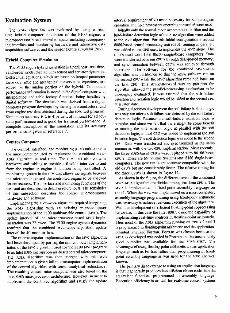
Evaluation System interval requirement of 40 msec necessary for stable engineoperation, multiple processors operating in parallelwere used.

The ADIA algorithm was evaluated by using a real- Initially only the normal-modeaccommodation filter andthetime hybrid computer simulation of the F100 engine, a hard-failure detection logic of the ADIA algorithm were addedmicroprocessor-basedcontrol computer includingaccompany- to the MVCalgorithm. For this initial configuration a seconding interface and monitoring hardware and interactive data 8086-basedcentral processing unit (cPu), running in parallel,acquisition software, and the sensor failure simulator (SFS). was added to the cPu used to implement the MVCalone. The

CPU's used were Intel 86/30 single-board computers. DataHybrid Computer Simulation were transferred between cPu's through dual-ported memory,

The F100 engine hybrid simulationis a nonlinear, real-time, and synchronization between cPu's was achieved through32nd-order model that includes sensor and actuator dynamics, interrupts. The software for the combined MVC-ADIA

algorithm was partitioned so that the ADIA software ran onDifferential equations, which are based on lumped-parameter the second cPu while the MVCalgorithm remained intact onthermodynamic and mechanical conservation equations, are the first cPu. This straightforward way to partition thesolved on the analog portion of the hybrid. Component algorithm allowed the parallel-processing mechanism to beperformance informationis stored in the digital computer with thoroughly evaluated. It was assumed that the soft-failureinterpolation and table lookup functions being handled by detection and isolation logicwould be addedto the secondcPwdigital software. The simulation was derived from a digital at a later date.computer program developed by the engine manufacturer and During algorithmdevelopmentthe soft-failureisolation logicfrom engine test data obtained during the MVCtest program.Simulation accuracy is 2 to 4 percent of nominal for steady- was only run after a soft failurewas detectedby the soft-failurestate performance and is good for transient performance. A detection logic. Because the soft-failure isolation logic iscomplete description of the simulation and its accuracy complex and since we felt that there might be some benefit

to running the soft isolation logic in parallel with the softperformance is given in reference 7. detection logic, a third cPu was added to implement the soft

isolationlogic. The softdetectionlogic was addedto the secondControl Computer cPu. Data were transferred and synchronized in the same

The control, interface, and monitoring (CIM) unit contains manner as with the two-cPu implementation. Most recently,the microcomputer used to implement the combined MVC- the three 8086-based cPu's were replaced with 80186-basedADIAalgorithm in real time. The CIMunit also contains CPU's. These are Monolithic Systems MSC8186 single-boardhardware and cabling to provide a flexible interface to and computers. The new cpu's are software compatible with thefrom the engine or engine simulation being controlled. A old cPu's but are considerably faster. The relative timing formonitoring system in the CIM unit allows the signals between the three cPu's is shown in figure 11.the microcomputer and the controlled engine to be checked As shown in the figure, the different parts of the combinedfor correctness. The interface and monitoring functions of the MVC-ADIAalgorithm are divided among the three cPU'S. TheCIMunit are described in detail in reference 8. The remainder MVCis implemented in fixed-point assembly language onof this subsection describes the control microcomputer cPu 1. When the MVCwas implementedon a microcomputer,hardware and software, assembly language programming using fixed-point arithmetic

Implementingthe MVC-ADIAalgorithm required integrating was necessary to achieve real-timeexecutionof the algorithm.the ADIA algorithm with an existing microcomputer With thedevelopmentofefficientfloating-pointcoprocessingimplementationof the F100 multivariable control (MVC).The hardware, in this case the Intel 8087, came the capability ofupdate interval of the microprocessor-based MVCimple- implementing real-time controls in floating-point arithmetic.mentation was 22 msec. The FI00 engine system dynamics Thus most of the ADIAalgorithm running on cPu's 2 and 3required that the combined MVC-ADIA algorithm update is programmed in floating-pointarithmetic and the application-interval be 40 msec or less. oriented language Fortran. Fortran was chosen because the

The microcomputer implementation of the MVCalgorithm ADIAas developed was coded in Fortran and because a fairlyhad been developed by porting the minicomputer implemen- good compiler was available for the 8086-8087. Thetation of the MVCalgorithm used for the F100 MVCprogram advantagesof using floating-pointarithmeticand an applicationto an Intel 8086 microprocessor-basedcontrol microcomputer, language such as Fortran rather than programming in fixed-The ADIA algorithm was then merged with this MVC point assembly language as was used for the MVCare wellimplementation to give a full microcomputer implementation known.of the control algorithm with sensor analytical redundancy. The primary disadvantage to using an application languageThe resulting control microcomputer was also based on the is that it generally produces less efficient object code than theIntel 8086 microprocessor architecture. However, in order to equivalent functions programmed in assembly language.implement the combined algorithm and satisfy the update Execution efficiency is critical for real-time control systems

INPUT-_ 60 --

' _ //-SCALEI /-SCALEO [] EXECUTIVE

_///-MVCP2 50-- _ ALGORITHM

CPU] /-OUTPUT

_,,, "_i-N_ _ 40-- [] MINDS, M NDS,' I''" ' ' ,_. 3o

CPU 2 EMODEL _: 20I I I I I

': 10/-ITRANS

CPU 3 FDISOL FDISOL 0

CPU I CPU 2 CPU 3 TOTALI I I I I

0 4 8 12 16 20 24 28 52 36 40TIME,MSEC Figure 13.--MVC-ADIA memory requirements. Algorithm code requires

65 percent of total algorithm memory. Total memory, 110 kilobytes.

CPU1INPUT A/D CONVERSIONAND SCALINGOF ENGINEMEASURE- access anyvariableintheMVC or ADIA algorithm.The data

MENTS taken can be uplinked to a mainframe computer for off-lineSCALEI CONVERSIONOFMEASUREMENTSTOFLOATINGPOINT processing.Inaddition,thesoftwarehasbeenenhancedtoAND TRANSFERTO CPU 2

MVCPI MVCPARTI: REFERENCEPOINTSCHEDULE,TRAN- allowplottingoftransientdataon-linewhilethecontrolSITIONCONTROL,ANDGAINSCHEDULECALCULATIONS microcomputerisoperating(ref.12).The on-linetransient

MINDS INTERACTIVEDATASYSTEM(SPARETIME CALCULA- datadisplayofinternalMVC and ADIA variableswas anTION)

SCALEO TRANSFEROF ESTIMATESAND RECONFIGURATIONIN- indispensabletoolintheevaluationprocess.

FORMATIONFROMCPU 2 AND CONVERSIONTO FIXED The memory requirements for each of the three cpu's are

POINT shown in figure 13. Each CPUhas, in addition to its share ofMVCP2 MVC PART2: PROPORTIONALCONTROL,INTEGRAL

CONTROL,ANDENGINEPROTECTIONLOGIC the MVC-ADIAalgorithm, an executive routine that maintainsOUTPUT UNSCALINGAND D/A CONVERSIONOF ENGINEINPUTS correctreal-timeoperationofthetotalalgorithm.Thememory

CPU2 requirements for the algorithm and for the executiveare shownEMODEL ENGINEMODELMATRIXAND BASEPOINTCALCULATIONETRANS TRANSFEROF EMODELINFORMATIONTO CPU 3 foreachcPu.Inaddition,thememoryrequirementforMINDSFDIA ACCOMMODATIONFILTERANDHARDDETECTIONLOGIC is shown for cpu 1. In all cases the code and the constants

CALCULATIONS were about 65 percent, and the data and the variables aboutINLET MACHNUMBERAND ALTITUDECALCULATIONCPU5 35 percent, of the total memory required. Lastly figure 13

FDISOLHYPOTHESISFILTERSANDSOFTISOLATIONLOGIC showsthetotalmemoryrequirementsforallexecutives,theCALCULATIONS total algorithm, and MINDSfor all three cPu's combined.ITRANS TRANSFEROF SOFTISOLATIONINFORMATIONTOCPU 5

Sensor Failure SimulatorFigure 12.--ADIA timing for 8-MHz MSC8186.

The sensor failure simulator (SFS)provides an efficient

including the MVC-ADIA. Thus for the ADIA,table lookup meansof modifying enginesensor signals to simulate sensorroutines, which are written to take advantageof the 8087 failures. The SFSunitconsistsof a personalcomputerdrivingarchitecture (ref. 9) and are executed frequently in the discrete analog hardware. The personal computer allows aalgorithm, and the hardware interfaceroutines, which have menu-driven,top-downapproachto failurescenarioretrieval,no Fortranequivalent,areimplementedin assemblylanguage, creation, editing,andexecution.The SFScan simulateany ofTo allow the remainderof the algorithmto remainin Fortran, four basic sensor failure modes: scale-factor change, bias,the source code has been optimized to make it run more drift, and noise. These failure modes are implemented inefficiently (ref. 10). As shown in figure 12, the entire analog electronic hardware that is controlled by the personalMVC-ADIA algorithm now executes in less than the required computer. The SFSallows complete and repeatable control40 msec. over the failure size and the timingof failure injection. Details

The programs for each of the cpu's are downloaded into of the SFSare given in reference 13.the cPU'S by using a commercially available disk operatingsystem, CP/M-86. The Microcontroller INteractive DataSystem (MINDS)is used for data acquisition (ref. 11). This Real-Time Evaluationsoftware runs on cPU 1 in the spare time when the cPU is notexecuting the MVCalgorithm (fig. 12). The package has both This section describes the evaluation of the ADIAalgorithmsteady-state and transient data-taking capabilities and can using a hybrid-computer-based, real-time simulation of an

10

F100 engine. The objectives, the procedure, and the results (altitude/Mach number) used during the evaluation are acrossof the evaluation are discussed, the top of the matrix, and the different tests conducted at these

points are along the side. Both MVConly and ADIA-MVC

Objectives evaluation tests are shown.Operating conditions.--The rationale used in selecting the

The first objective of the evaluation was to validate the test matrix operating conditions was to duplicate as manyoperation and performance of the ADIAalgorithm and its conditions as possible used in the F100 Multivariable Controlimplementation. It was especially important to conduct this Program (ref. 6), to avoid high fan inlet pressures, and tovalidation in a real-time environment in order to establish the reasonablyspanthe envelope. This rationalewas a compromisefeasibility and practicality of the implementation. The second between taking advantage of previous results for comparison,objective was to document the performance of the algorithm limited-riskengine operation,and full-envelopevalidation.Theover the envelope of the engine. The third objective was to testconditions selected are plottedon the engine face conditionestablish a data base for comparison with results obtained envelope in figure 14.during the demonstration phase of the program. Test definitions.--The tests used in the evaluation were

selected to completely define detection performance for fivecommon failures modes. Also, tests were conducted to

Procedure determine engine control performance with and without theThe procedure for evaluating the algorithm is defined by ADIA algorithm and with and without engine sensor failures.

the test matrix (table II). The different operating conditions The tests are summarized in table III.

TABLE II.--EVALUATION TEST MATRIX

Test Operating condition,altitude (1000 ft)/Mach number

10/0.6 30/0.9[ 10/0.9[ 45/0.9[ 10/1.2 50/1.8 , 35/1.9 I 55/2.2

Number of tests

Sensor failure test:Hard 10Soft 10 10 10 5 5 5 5 5Drift 10 10 10 5 5 5 5 5Noise 2 2Scale 2 2Sequence 12 12Pulse 1 1 1 1 1

Open 1 1Random 4 4Frequency 4 4

MVCtests:MVCSS 7 3 3 3 2 1 1 1MVCpulse 1 1 1 1 1Original/CIM 1 1. 1 1 1comparison

Single 5

11

TABLE III.--TEST DEFINITIONS

Test Description

ADIA-MVCevaluation

Hard Large bias failureSoft Small bias failureDrift Small drift failure

Noise Random noise failure 60 --Scale Scale-factor bias changeSequence Sequence of successive output sensor failuresPulse Minimum-to-maximum-to-minimum transient power _-

excursions. Maximum power level is maintained for 10 sec.Open Same as pulse test except that minimum power level is

o.

raised slightly, maximum power level is decreased slightly, __ qO -- OPERATINGPOINT,and engine is controlled without using any sensed engine _ ALTITUDE(1000 FT)/output information, ua_ MACHNUMBER

10/1 0

MVC-onlyevaluation _°_ 20-- 10_ O 35/1.9

MVC Same as pulse test except that control is run exclusively with _ /0.6,L'7 - O 55/2.2engine sensed output. ADIA estimates are not used - 10 f_ O 50/1.8in control. _ /O 30/0.9

MVCSS Steady-state data at operating point 0 _-- O 45/_..9 I_"-"-'_ I IBleed Pulse test with bleed control disabled 400 500 600 700 800 900Single Pulse test with single sensor failure accommodated before FANINLETTEMPERATURE,TT2o OR

initiating transientAlt/Mach Altitude/Mach number excursion from 10000 ft/Mach 0.6

to 45 000 ft/Macb 0.9 Figure 14.--Evaluation test conditions.

Results demonstrated that the microprocessor-based implementationof the MVCcontrol algorithm could accurately and safely

Three types of real-time evaluation results are presented, control the test-bed engine. Steady-state and transient resultsThe first shows the performance of the microprocessor-based were obtained at the testmatrix operating conditions. In everyMVCcontrol. The second shows the accuracy of the Kalman- case both the steady-state and transient accuracy results werefilter-based estimator. Finally the performance of the ADIA good. The steady-state results are summarized in table IV.algorithm itself is given. Minimum and maximum steady-state error results at seven

MV€performance.--The performance of the MVC control points in the 10 000-fi/Mach 0.6 operatingcondition are givenwas evaluated without the ADIAlogic. This evaluation graphically in figure 15 for N1 (minimum error) and in

TABLE IV.--STEADY-STATE MVC PERFORMANCE RESULTS

Operating condition Engine output

Altitude, Mach Power N1 N2 PT4 PT6 FTIT EPR

ft number lever

angle, Value, percent of nominalPLA,deg

10×103 0.6 50 0.07 0.66 1.94 -0.18 6.71 -0.79.6 83 -.40 .08 -.31 -.48 .24 1.53.9 50 -.17 -.36 -2.66 .00 1.49 .13.9 83 - .72 .17 .75 - .07 - .41 - .07

1.2 70 -.08 - .21 -. 15 - 1.35 .32 -.0730 .9 50 -.07 -.52 -. 11 -.37 7.20 - 1.39

.9 83 .09 -.20 .94 -.24 1.16 -.2435 1.9 83 -.34 -.31 -2.47 -.86 -1.96 -.5145 .9 70 -.16 -.31 0 -.71 -9.89 -1.4550 1.8 83 -1.20 -2.01 -5.50 -2.18 -3.78 -1.9355 2.2 83 .28 1.37 4.97 .11 .81 .11

12

llxl_O3-h SCHEDULED0 SENSED

• ESTIMATED "_)I0 -- 1800--

Jr SCHEDULED __)0 SENSED

9 -- "_) 1600-- • ESTIMATED

{ 8- -_ _ 14oo-taJ

7 _ _ 12oo- Q +

- +6 -- _ 1000 -- Q

==+

5 -- 800 --

I I I I I I I 6oo I I I I I I I20 30 40 50 60 70 80 90 20 30 40 50 60 70 80 90

POWERLEVERANGLE,DEG POWERLEVERANGLE,DEG

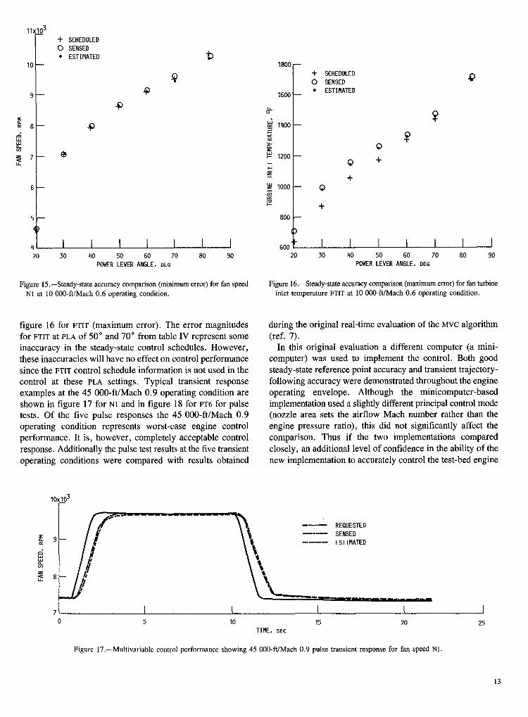
Figure 15.--Steady-state accuracycomparison (minimumerror) forfan speed Figure 16.--Steady-stateaccuracycomparison(maximumerror)forfanturbineN1 at 10 000-_/Mach 0.6 operating condition, inlet temperature FTIT at 10000-_/Mach 0.6 operating condition.

figure 16 for FTIT(maximum error). The error magnitudes during the original real-time evaluation of the MVC algorithmfor FTITat PLAof 50° and 70° from table IV represent some (ref. 7).inaccuracy in the steady-state control schedules. However, In this original evaluation a different computer (a mini-these inaccuracies will have no effecton control performance computer) was used to implement the control. Both goodsince the FTIT control schedule information is not used in the steady-state reference point accuracy and transient trajectory-control at these PLA settings. Typical transient response followingaccuracy were demonstrated throughout the engineexamples at the 45 000-ft/Mach 0.9 operating condition are operating envelope. Although the minicomputer-basedshown in figure 17 for N1and in figure 18 for PT6for pulse implementationused a slightlydifferent principal control modetests. Of the five pulse responses the 45 000-ft/Mach 0.9 (nozzle area sets the airflow Mach number rather than theoperating condition represents worst-case engine control engine pressure ratio), this did not significantly affect theperformance. It is, however, completely acceptable control comparison. Thus if the two implementations comparedresponse. Additionallythe pulse test resultsat the five transient closely, an additional level of confidence in the ability of theoperating conditions were compared with results obtained new implementation to accurately control the test-bed engine

lOxlO3

-- REQUESTEDSENSED

9 ESTIMATED

5o-)

8

7 [ I L [ I0 5 10 15 20 25

TIME, SEC

Figure 17.--Multivariable control performance showing 45 000-ff/Mach 0.9 pulse transient response forfan speed N1.

13

I I I I0 5 10 15 20 25

TIME, SEC

Figure 18.--Multivariable control performance showing 45000-fi/Mach 0.9 pulse transient response for exhaust nozzle pressure PT6.

9750--

9500 -- | Ii9250 --

REQUESTED----- MVC/ADIA

MVC/ORIGINAL

9000 --

8750 --

+oo- I8250 -- t

I!

8000 -- I!

I!

7750 -- I

7500 -- _"---"_ "" ----_"" --"

7250 I I I I I5 10 15 20 25

TIME, SEC

Figure 19.--Multivariable control response to 45 000-ft/Mach 0.9 pulse transient for fan speed Nl--comparison for two implementations.

14

12[-11

-- REQUESTED

----- MVC/ADIA

MVC/ORIGINAL

10

N

s I I I I I0 5 10 15 20 25

TIME, SEC

Figure 20.--Mu]tivariable control response to 45 O00-ft/Mach 0.9 pulse transient for augmentor pressure PT6--comparison for two implementations.

12_ 3REQUESTED

10 ----- SENSED

ESTIMATED

4O

III

II

_"30

__oII

15

10 I I I I (">10 5 10 15 20 25

TIME, SEC

(a) N] pulseresponse.(b) PT6 pulse response.

Figure 21 .--ADIA-MVC performance at 10000-ft/Mach 0.6 operating condition.

15

12xlO3

FREQUESTED

10 SENSED

ESTIMATED

,,a,8

O3

6

40

lo I 1 I I0 5 10 15 20 25

TIME, SEC

(a) NI pulse response.(b) PT6 pulse response.

Figure 22.--ADIA-MVC performance at 10 000-ft/Mach 0.6 with a PT6 sensor failure.

systemwas obtained.As seenin the typicalresponsesof figure 19 Control performance was also evaluated given that a singlefor N1and in figure 20 for PT6,the comparisonwas quitegood. sensor failure had occurred. The purpose of this test was toThis wastypicalfor all fiveof the transienttestmatrixconditions, evaluate control performance after a single sensor failure had

Additionally the control was evaluated to determine if been accommodated. In this case five pulse transients at thesuccessful engine operation could be obtained without com- 10 000-ft/Mach 0.6 operating condition were simulated. Inpressor bleed. In these tests the simulation was subjected to each case a single, but different, output sensor failure wasthe pulse transientwith the compressorbleed fixedin the closed accommodated before the pulse transient was initiated. Theposition. The transient was simulated at the 10 000-ft/Mach normal-moderesponses and the failure transient responses are0.6 operating condition. These results were compared with compared for an N1failure in figure 21 and for a PT6 failurethose for the nominal configuration. The comparison shows in figure22. Control performance was good for all five failure-no discernible difference between engine control operation mode cases. Additional information about estimate accuracywith and without compressor bleed, during these tests is given in the next section.

16

50_

60 40 --

_30--i,_ 40 OPERATINGPOINT.ALTITUDE(1000FT)/

_ MACHNUMBER

_ 10/1 ,_20I0/0,920

_ 10

o I _^>1 I I 1 I (_>1400 500 600 700 800 900 0 5 10 15 20 25

FAN INLET TEMPERATURE,TT2, OR TIME, SEC

1.0

5 10 15 20 25TIME, SEC

(a) Model operating points for PT2/TT2 envelope.(b) Altitude excursion.

(c) Mach number excursion.

Figure 23.--Altitude and Mach number excursions.

10,42103

_-- _ REQUESTEDSENSED

--_",._Z_..._. ESTIMATED

{

I0.0--

9._ I I I I I5 10 15 20 25

TIME, SEC

Figure 24,--ADIA-MVC performance--N1 response to altitude and Mach number excursions of figure 23.

Finally control performance was evaluated for an altitude the 45 000-ft/Mach 0.9/83 ° operating condition as shown inand Mach number excursion. The ADIA-MVC control figure 23. Data showing N1 and PT6 control for this transientperformed acceptably during this excursion. The excursion are given in figures 24 and 25, respectively. Controlwent from the 10 O00-ft/Mach0.6/83" operating condition to performance for this transient was quite good.

17

50

45

REQUESTED_ SENSED

40 ESTIMATED

35G

o..

_ 30

2s

20

15

lo I I I I I0 5 10 15 20 25

TIME,sEc

Figure 25.--ADIA-MVC performance--PT6 response to altitude/Mach number excursions of figure 23.

Estimator accuracy.--The single most important elementin determining ADIA algorithm performance is the accuracyof the engine output estimates used in the algorithm, Theseestimates are determined by the accommodation filter, whichincorporates a simplified engine model. The accuracy of the TABLE V.--STEADY-STATE ESTIMATION ACCURACY

output estimates for both steady-state and transient operation RESULTS WITH NO SENSOR FAILURES

was evaluated at various engine operating conditions. AnOperating condition Engine output

engine operating condition is defined by the pilot's power

request (power lever angle, PLA)and the altitude (ALT)and Altitude, Mach Power NI N2 I PT4 ]PT6 ]FTITMach number (MN) at which the engine is operating. The ft number leveraccuracy of the estimates is presented in two parts, steady- angle, Accuracy,percentof nominal

state accuracy and transient accuracy. PLA,Steady-state accuracy was obtained in a straightforward deg

manner. The simulationwas "flown" to the desired operating 10× 103 0.6 83 0.43 0.11 3.16 0.53 0. I 1

condition and allowed to reach steady state. Then control 30 .9 50 .06 .16 .21 1.53 .11

execution was halted (or frozen). MINDSwas then used to 10 .9 83 .42 .28 1.36 .69 .04sample and store a set of steady-state data. Measured and 45 .9 60 .12 .21 t.87 1.45 .0410 1.2 83 .17 .11 1.36 .33 .11estimated variables for seven operating conditions are 55 2.2 _ .33 .54 5.64 2.48 .05compared in table V by showing the difference (the residual) 35 1.9 | .03 .32 .92 5.12 .01between sensed and estimatedfan speedN1, compressor speed 50 1.8 _ .39 .49 3.12 2.48 .04N2, combustor pressure PT4,exhaust nozzle pressure PT6,andfan turbine inlet temperature FTIT as a percentage of the Average 0.24 0.28 2.21 1.83 0.06nominalvalue. Maximum .43 .53 5.64 5.12 .11

18

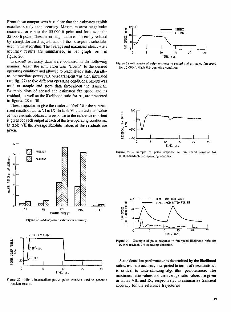
From these comparisons it is clear that the estimates exhibitexcellent steady-state accuracy. Maximum error magnitudes 12I_L0_3

occurred for PT4 at the 55 000-ft point and for PT6 at the i :__- ESTIMATESENSED

35 000-ft point. These error magnitudescan be easily reduced , 1 - /_'--'--_"xby straightforward adjustment of the base-point schedules J, ,used in the algorithm. The average and maximum steady-state _ _1 Iaccuracy results are summarized in bar graph form in 0 5 10 15 20 25figure 26. TIME.SEC

Transient accuracydata were obtainedin the following Figure 28.--Example of pulse response to sensed and estimated fan speedmanner: Again the simulation was "flown" to the desired for 10000-fl/Mach 0.6 operating condition.operating conditionand allowed to reach steady state. An idle-to-intermediate-power PLApulse transient was then simulated(see fig. 27) at five different operating conditions. MINDS wasused to sample and store data throughout the transient.Example plots of sensed and estimated fan speed and itsresidual, as well as the likelihood ratio for N1, are presentedin figures 28 to 30.

These trajectories give the reader a "feel" for the summa-

rized results of tables VI to IX. In table VI the maximum value _ 200of the residuals obtained in response to the reference transient

is given for each output at each of the five operatingconditions. _ _ 0In table VII the average absolute values of the residuals are•_ -200

given. R

-,00 I I I I0 5 10 15 20 25

6- TIME,SEC

F_ AVERAGE _"Q Figure 29.--Example of pulse response to fan speed residual for5

F,,\',_ _ 10000-ft/Mach 0.6 operating condition.D MAXIMOM..,.,z ....-

v//I -- _\" v//

F-- TCTIO.THRESHOLD_ I_///_,, .,,, o .... LIKELIH00DRATIOFORN10 ,_',Y/A, \\" _ _.

NI N2 PT4 PT6 FTIT _ _: .8ENGINEOUTPUT u_

=i::

Figure 26.--Steady-state estimation accuracy. _ "4

..J

0 5 10 15 20 25

.-- INIERMEDIAIE TIME, SEC

_, Figure 30.--Example of pulse response to fan speed likelihood ratio for10O00-ft/Mach 0.6 operating condition.

"_ 1260/SEC

_J

_._f" IDLE Sincedetection performance is determinedby the likelihood20 I I I J ratios, estimate accuracy interpreted in terms of these statistics0 s 10 15 20 is critical to understanding algorithm performance. TheTIME,SEC

maximum ratio values and the average ratio values are givenFigure27.--Idle-to-intermediate power pulse transient used to generate in tables VIII and IX, respectively, to summarize transient

transientresults, accuracy for the reference trajectories.

19

TABLE VI.--MAXIMUM RESIDUAL VALUE IN TABLE IX.--AVERAGE LIKELIHOOD RATIO INRESPONSE TO PLA PULSE INPUT RESPONSE TO PLA PULSE INPUT

(NORMAL MODE) (NORMAL MODE)

Operating condition Engine output Operating condition Engine output

PT6 I FTIT Altitude, Mach N1 N2 PT4 PT6 FTIT

F

Altitude, Mach N1 N2 PT4fi number I ft number

Value, percent of nominal Average likelihood ratio

10x103 0.6 3.57 0.81 6.50 12.55 5.78 10x103 0.6 0.086 0.057 0.044 0.059 0.01030 .9 1.47 .74 4.48 13.08 5.49 30 .9 .060 .037 .006 .045 .00710 .9 4.30 1.13 5.22 14.98 5.68 l0 .9 .088 .047 .038 .123 .01045 .9 2.89 1.86 7.81 19.30 4.44 45 .9 .044 .034 .003 .007 .00710 1.2 1.54 1.24 5.02 9.21 3.50 10 1.2 .015 .107 .124 .020 .006

Average 2.75 1.16 5.81 13.82 4.98 Average 0.059 0.056 0.023 0.051 0.008Maximum 4.30 1.86 7.81 19.30 5.78 Maximum .088 .107 .044 .123 .010

Plots of the likelihood ratios became the standard tool usedTABLE VII.--AVERAGE RESIDUAL ABSOLUTE VALUE

INRESPONSETO PLA PULSE INPUT for evaluation and performance prediction. Transient accuracy(NORMAL MODE) was considered to be quite good overall although not as good

as steady-state accuracy. It was fairly evident then that

Operating condition Engine output detection performance could be greatly improved if different

I thresholds for steady-state and transient detection wereAltitude, Mach NI N2 PT4 PT6 FTIT

ft number allowed. This observation led immediately to the implemen-Value,percentof nominal tation of the adaptive threshold logic described earlier.

Estimatoraccuracy resultswere also obtained for the single-10xl03 0.6 0.77 0.24 1.67 2.33 1.44 failure pulse tests described in the MVCevaluation. These30 .9 .63 .28 .92 2.94 1.64 results are given in table X for maximum residual values and10 .9 .60 .42 .78 2.98 1.3945 ,9 .49 .36 2.37 5,78 1.21 in table XI for average residual values. These tests show very10 1.2 ,21 .23 1.21 .75 .85 littledegradationinestimator accuracyperformance even when

it was operating with only four sensors. Thus ADIA perfor-

Average 0.54 0.31 1.39 2.96 1.31 mance will not degrade significantly after a single sensorMaximum .77 .42 2.37 5.78 1.64 failure.

Estimator accuracy was also studied during the altitude/Mach number excursion of figure 23. As an example sensedand estimated N1 and PT6 are compared in figures 24 and 25,respectively. In each case the accuracy was excellent.

TABLE VIII.--MAXIMUM LIKELIHOOD RATIO INRESPONSE TO PLA PULSE INPUT

(NORMAL MODE)TABLE X.--MAXIMUM RESIDUAL ERRORS FOR PULSE

Operating condition Engine output TRANSIENTS AT 10 000 FT/MACH 0.6 WITHSINGLE SENSOR FAILURE

Altitude, Mach N1 N2 PT4 PT6 FTIT

ft number Output Failure modeMaximum likelihood ratio

None N1 N2 PT4 PT6 FTIT10× 103 0.6 0.875 0.342 0.286 0.598 0.08030 .9 .241 .146 .076 .305 .042 Maximum residual error10 .9 1.025 .236 .162 1.340 .05945 .9 .400 .238 .009 .059 .042 NI 3.570 0 2,931 2.592 2.481 2,87710 1.2 .126 .253 .355 .401 .041 N2 .810 .979 0 .823 .784 .791

PT4 6.500 7.513 5.211 0 6.454 6.550Average 0.533 0.243 0.177 0,540 0.053 PT6 12.550 10.740 12.220 11.480 0 11.880

Maximum 1.025 .342 .355 1.340 .080 FTIT 5.780 6.383 5.704 5.650 5.731 0

20

TABLEXI.--AVERAGE RESIDUALERRORSFOR PULSE TABLE XII--MINIMUM BIAS FAILURE MAGNITUDESTRANSIENTS AT 100!30FT/MACH 0.6 WITH

SINGLE SENSOR FAILURE (a) Units

Operating condition Engine outputOutput Failure mode

Altitude, Mach Power N1, N2, PT4, PT6, FTIT,

None NI N2 PT4 PT6 FTIT ft number lever rpm rpm psi psi °Fangle,

Average residual error PLA, Failure magnitudedeg

N1 0.770 0 0.755 0.472 0.571 0.483

N2 .240 .249 0 .250 .265 .270 10× 103 0.6 50 300 300 12.50 3.00 150PT4 1.670 1.479 .693 0 1.067 1.260 .6 83 350 350 12.50 3.00PT6 2.330 2.211 2.486 2.432 0 2.431 30 .9 50 300 13.50 2.75FTIT 1.440 1.305 1.417 1.406 1.455 0 83 325 13.50 3.00

10 50 300 13.50 2.7583 300 " 11.00 3.00

45 " 70 200 400 18.00 3.00 250Detection, isolation, and accommodation performance.-- 10 1.2 70 200 400 20.00 3.50 150

Two types of sensor failureswere considered:hardandsoft. 50 1.8 83 300 350 12.50 3.00 |Hardfailures, becauseof theirsize, areeasily detected.Thus 35 1.9 83 300 300 19.00 3.00

hard-failure detection performance, although important to 2.2 83 250 500 25.00 3.00

systemreliability, was examined at only one operating condi- (b) Nominaltion. The ADIAalgorithm exhibited excellent hard-failuredetection performance at this condition. There were no false Operatingcondition Engineoutput

alarms or missed detections of any hard failures at the oper- Altitude, Mach Power N1 N2 PT4 PT6 FTITating condition studied. Hard failures were simulated in each ft number lever

of the engine sensor outputs. The failure was successfully angle,detected and accommodated in each case. In addition, no false PLA, Failure magnitude,alarms in the hard-failure detection logic were encountered deg percent of nominal

during the subsequent soft-failure evaluation. 10×103 0.6 50 3.47 2.60 6.39 12.02 12.00Soft sensor failures, although small in magnitude, if .6 83 3.41 2.67 3.85 7.74 8.75

undetected, may result in degraded or unsafeengine operation. 30 .9 50 3.43 3.10 10.92 18.10 12.36Soft failures are more difficult to detect. Therefore the 83 3.25 2.73 6.99 13.24 9.41

evaluation concentrated on soft-failure detection and isolation 10 50 3.54 2.60 6.17 9.74 12.1783 2.91 2.66 2.86 6.40 8.72

performance. Four soft-failure modes were considered: bias, 45 ', 70 2.12 3.34 21.33 29.96 18.18drift, noise, and scale factor. Algorithm performance for 10 1.2 70 2.11 3.21 5.71 7.78 10.00the bias and drift failure modes was studied extensively. 50 1.8 83 2.94 2.71 8.33 17.44 9.06Performance for the noise and scale-factor modes was studied 35 1.9 83 2.95 2.31 5.94 7.69 8.94at a limitednumber of conditions. Performancecriteria studied 55 2.2 83 2.57 3.76 16.34 15.54 8.80

were minimum detectablebias values and drift rates, detection (c)Full-scalebiastime, steady-state performance degradation, and transientresponse to failure accommodation. Operating condition Engineoutput

The procedure followed to obtain performance data was Altitude, Mach Power NI N2 PT4 PT6 FTITidentical to that used to obtain transient accuracy data. ft number lever

Additionally the SFSwas used to simulate a sensor failure of angle,the appropriate size and at the desired time. The results PLA, Failure magnitude,obtained are summarized for the minimum detectable level of deg percent of full scale

bias in table XII. lOx103 0.6 50 2.92 2.29 3.85 7.74 8.75In table XII the minimum detectable biases at 11 different .6 83 3.41 2.67 3.85 7.74

operating conditions for each engine output are given. The 30 .9 50 2.92 2.67 4.15 7.1083 3.17 2.67 4.15 7.74detection times for the minimumdetectable biases were essen-

10 50 2.92 2.29 4.15 7.10tially instantaneous. The results are presented as a percentage 83 2.92 2.67 3.38 7.74 ,'of full scale, a percentageof nominal, and in engineeringunits. 45 , 70 1.95 3.05 5.54 7.74 4.59

Full-scale values are constant, but nominal values can vary 10 1.2 70 1.95 3.05 6.15 9.04 8.75

throughout the operating range. Note that the size of the 50 1.8 83 2.92 2.67 3.85 7.74 |

failures detected (in units or equivalently as a percentage of 35 1.9 83 2.92 2.29 5.85 7.7455 2.2 83 2.44 3.81 7.69 7.74full scale) was essentially constant over the operating range.

21

50--

D AVERAGE _ TABLE XIII.--MINIMUM DRIFT FAILURE MAGNITUDES25

#: --D MAXIMUM _\.,, (a) Units

20 -- _ _ Operating condition Engine output

_N'--_ Altitude, Mach Power NI, N2, PT4, PT6, FTIT,...... \\\ fl number lever rpm/sec rpm/see psi/see psi/see °F/seeI"" " \" \ angle, '

• \\\ \_.\10 -- \\\ _ _\,_'_ PLA, Failure magnitudev / / ,,\,, deg

\\\ V/I \\\

5 ?_._ \\\ v// \\-,v// \., 10X 103 0.6 50 100 100 2.50 0.80 70\ \\ 11"// \\\"-\" t/// ,\\ .6 83 125 125 1.25 .60

v// 30 .9 50 130 100 2.50v//0 "_] ] 83 150 125 3.00

NL NH PTtl PT6 FTIT 10 50 100 100 2.50ENGINEOUTPUT 83 125 125 2.00 ,

45 " 70 100 150 3.00 .80 75

Figure 31.--Minimum detectable bias failure. 10 1.2 70 25 150 3.50 1.20 7050 1.8 83 150 150 1.75 .20 70

35 1.9 83 125 50 3.00 .20 70

Note also that the highest detectable bias (29.96 percent) as 55 2.2 83 75 215 4.50 .60 75a percentage of nominal occurred for PT6 at 45 000-ft/Mach0.9/70 ° because of the low nominal value of PT6 at this (b)Nominaldrift

condition. However, this failure as a percentage of scale (7.74 Operatingcondition Engine output

percent) was about average. The minimum detectable bias I I

Altitude, Mach Power N1 I N2 PT4 ] PT6 FTITmagnitudes were small overall and represented excellent ft number leverperformance.Thisperformanceis summarizedin bar graph angle,form in figure 31. PEA, Failure magnitude, percent of nominal

degThe minimum detectable drift rates (table XIII) were

determined by adjusting the drift magnitude such that a failure lOx103 0.6 50 1.16 0.87 1.28 3.20 5.60was detected approximately5 sec after its inception. As in the .6 83 1.22 .95 .38 1.55 4.08

30 .9 50 1.49 .89 2.02 3.95 5.77bias case the highest minimum detectable drift rate as a 83 1.50 .97 1.55 2.65 4.39percentage of nominaloccurred at the 45 000-ft/Mach 0.9/70 ° 10 50 1.18 .87 1.14 2.13 5.68operating condition. However, as before, this value as a per- 83 1.21 .95 .52 1.28 4.07

45 _ 70 1.06 1.25 3.55 7.99 5.45centage of nominal was well below the maximum value as a 10 1.2 70 .26 1.20 1.00 2.67 4.67percentage of full scale. The percentage-of-full-scale values 50 1.8 83 0 .01 .01 .03 .05are all similar in magnitude. In general these results, which 35 1.9 83 1.23 .38 .94 .51 4.17

55 2.2 83 .77 1.61 2.94 3.11 4.40are summarized in the bar graph of figure 32, were excellent.

(c) Full-scale drift

8 -- _ Operating condition Engine outputi

D k\x,.\\AVERAGE "-\ \ Altitude, Mach Power N1 N2 P ['4 PT6 FTIT_.._," ft number lever

,,=5,6- U MAXIMUM _.'_'_ angle,0.. \\\ _ PLA, Failure magnitude, percent of full scale_d \\x ,xx

-...-- _N'K deg

z 4 ....... lOxlO 3 0.6 50 976 0.76 0.77 2.70 4.08

\\\ \\\" "" "\\ /._ .6 83 1.22 .95 .38 1.55• \\ \\\

\\', /,(, .\, 30 .9 50 1.27 .76 .77"-\', "-"-", 83 1.46 .95 .92\\\ \\\

2- _'_ ,,\\ 10 50 .97 .76 .77_.._-_ 83 1.22 .95 .62 ,'

+I E \\\ \\\ 45 70 .97 1.14 .92 2.07 4.38,,\\ \\'h 10 1.2 70 .24 1.14 1.08 3.10 4.08-,\-, 50 1.8 83 0 .01 .01 .03 .04

0 \\\ 35 1.9 83 1.22 .38 .94 .51 4.17NL NH pTtl PT6 FTIT 55 2.2 83 .73 1.64 1.38 1.55 4.38

ENGINEOUTPUT

Figure 32.--Minimum detectable ramp failure.

22

TABLE XIV.--STEADY-STATE RESULTS OF SLOW DRIFT FAILURE TRANSIENTS FOR ORIGINAL ADIA ALGORITHM

Operating condition Failure ADIAalgorithmparameter

Altitude, Mach Power Parameter bias Change in Time for Comments Performance aft number lever before DIA thrust DIA,

angle, before DIA, secPLA, percent

deg

0 0 24 P6 7.4 psi (42%) -4.5 0.490 A0 40 NI 1333 rpm (12.1%) -44.5 1.994 U0 83 PT4 46.5 psi (12.7%) --.1 3.080 Filter noisy during ADIA A1.2 83 FTIT 90 F (5.2%) -2.2 2.53 |

10× 103 .75 50 PT4 40.5 psi (19.6%) -.2 2.664

.75 83 PT6 9 psi (21.8%) --1.5 .57220 .3 40 N2 Undetected .... Undetected Unstable diverging U

.3 83 N2(-) Undetected .... Undetected Unstable U

.3 ! N2 1415 rpm (11.4%) -4.5 3.518 A25 1.0 / PT4 46.5 psi (18.1%) --.2 3.066 A

2.2 _' PT4 False alarm ........ PT4 and PT6 false alarms prior to failure U40 .6 40 N2 Miss -48 .... 2000-rpm drift miss U

.6 83 PT6 6.75 psi (63.7%) -.5 .448 System oscillatory after failure induced A45 2.2 / P4 -56.4 psi (-24.5%) -.16 3.750 A60 1.2 / N2 2000 rpm (15.8%) --19.4 5.016 Drift caused system to go unstable U65 2.5 _ P6 -3.75 psi (-27.4%) +24.7 .400 FTIT false alarm U

aA = acceptable; U = unacceptable.

To place these results in perspective, the soft-failure detect-ion performance of this improved version of the algorithm TABLEXV.--DRIFTFAILURERESULTSwas compared with the original algorithm (ref. 1). In thiscomparison drift failures were injected at 17 "edge of the Operatingcondition Failure Parameter Change in Time

parameter bias thrust forenvelope" points. Performance data for the original algorithm Altitude, Mach Power beforeDIA, DIA,(table XIV were obtained from a nonlinear, digital simulation ft number lever percent secof the engine. The performance of the improved algorithm is angle,

PLA,

presented for comparison in table XV. degSome of the operating conditions of table XIV are only

approximated in table XV. The hybrid computer could not 0 0 24 P6 3.7psi 0 0.5successfully attain these conditions because of scaling limita- 0 40 NI 263.0rpm 1 .30 83 PT4 15.2 psi 0 .9

tions. In every case but one, the improved version of the 1.2 83 FTIT 124.0°V -4 2.5algorithm had a smaller parameter bias before detection than 10×103 .75 50 PT4 16.4psi 0 .9

.74 83 PT6 2.7 psi -8 3.7the originalversion. In all failurecases the improved algorithm 20 .3 40 N2 248.0rpm -1 .3allowed continued engine operation; in some cases the original .3 83 iN2(-) -234.0rpm 1 .5algorithm would have required an engine shutdown. The drift .3 [ N2 265.0rpm - 1 .3failure rates used in this comparison are given in reference 1. 25 1.0 _ IPT4 16.8psi 0 1.02.0 PT4 17.8 psi -- 1 1.2

Estimation accuracy and false alarm performance were also 40 .6 40 N2 216.0rpm -5 .5evaluated for the altitude/Mach number excursion definedby .6 83 PT6 2.6psi - 11 1.6figure 23. Likelihood ratio and detection threshold responses 45 2.1 PT4 15.7psi 0 .560 1.2 N2 274.0 rpm -- 15 .8

are given in figure 33 for the PT4 and PT6 engine outputs. The 65 2.3 PT6 3.7psi -5 2.3likelihood ratios for N1, N2, and FTITwere all smaller than 45 2.1 " PT4(--) --15.0psi 0 1.5those for PT4 and PT6. Here the accuracy was quite good andthere were no false alarms.

23

Actuator Modeling Error Evaluation

The effectsof fuelflow actuatorand fuelflow feedbacksen-sor modelingerrors were also evaluated.Since the algorithmestimates depend on fuel flow informationand since fuelflow is the primary control variable, fuel flow actuationormeasurement errors could significantly degrade detection

,8 DETECTION performance. Likelihood ratio results for the PLApulse testTHRESHOLDPT_ at the 10 000-ft/Mach 0.6 operating condition are shown in

o .6 -- PT6 figure34 for normal operation, for operationwith a 10percent,_ change in the fuel flow actuator gain, and for operation with

a 10percent change in the fuel flow feedback measurement._.4 -- In each case no false alarms were encountered. In general,._ detection performance was not significantly degraded by the__ modeling errors. However, some effect was seen for a

•2 - feedback sensor error on the N2 and PT4 likelihood ratios. For

,_""_ PT4 the difference occurred only during an engine acceleration_/,.,,'.,._2__._.,j,.,_ I _ I, I and wouldhave onlya limitedeffecton detectionperformance.

5 10 15 20 25 For N2, however, a steady-state error occurred that in theTIME,SEC

worst case would result in approximatelya 50 percent increaseFigure 33.--Likelihood ratio response during altitude/Machnumberexcursion, in minimum detectable failure magnitudes.

1.2 -- DETECTIONTHRESHOLDNORMALMODE

SENSORERROR

1.0 ACTUATORERROR

2 f'\%

-.2 I I I I0 5 10 15 20 25

TIME, SEC

(a) N1 likelihood ratio.

Figure 34--Fuel flow modeling error effects for various likelihood ratios.

24

1.2DETECTIONTHRESHOLD

_-_ NORMALMODE.... SENSORERROR

.... ACTUATORERROR1.0

(c)

-.2 I I I I i0 5 10 15 20 25

TIRE, SEC

(b) N2 likelihood ratio.

(c) PT4 likelihood ratio.

Figure 34.--Continued.

25

1.2

"-"" DETECTIONTHRESHOLD

--'-- NORMALMODE.... SENSORERROR

1.0 ACTUATORERROR

.8

,2--

(E)

-. I I I I I0 5 10 15 20 25

TIME,SEC

(d) PT6 likelihoodratio.

(e) FTIT likelihood ratio.

Figure 34.--Concluded.

26

Conclusions and straightforward programming procedures, includingFortran and floating-point arithmetic, were used. Parallel

As a result of this real-time evaluation study several conclu- processing was also used and shown to be an effectivesions have been reached, multiplier of computational resources.

1. The advanced detection, isolation, and accommodation 3. The ADIA algorithm and MVCcontrol microprocessor-(ADEn)failure detection algorithmworks and works quite well. based implementationsare ready for demonstration. The ADIA

Sensor failure detection and accommodationwere demonstra- algorithm will be demonstrated on a full-scale F100 engineted over a broad range of operating conditions and power in the Lewis Research Center's altitude test facility.conditions. The minimum detectable failure magnitudesrepresent excellent algorithm performance.

2. The algorithm is implementable in a realistic computer Lewis Research Centerenvironment and in an update interval consistent with real- National Aeronautics and Space Administrationtime operation. Off-the-shelf microprocessor-based hardware Cleveland, Ohio, April 14, 1987

References

1. Merrill, W.C.: Sensor Failure Detectionfor Jet Engines UsingAnalytical Verification of a Real-Time, Hybrid Computer Simulation of theRedundancy. Journal of Guidance, Control and Dynamics, vol. 8, F100-PW-100(3) Turbofan Engine. NASA TP-1034, 1977.no. 6, Nov.-Dec., 1985, pp. 673-682. 8. DeLaat, J.C.; and Soeder, J.F.: Design of a Microprocessor-Based

2. Beattie, E.C., et al.: Sensor Failure Detection Systemfor F100 Turbofan Control, Interface, and Monitoring (CIM) Unit for Turbine EngineEngine. (PWA-5736-17, Pratt & Whitney Aircraft; NASA Contract Controls Research. NASA TM-83433, 1983.NAS3-22481) NASA CR-165515, 1981. 9. Mackin, M.A.; and Soeder, J.F.: Floating-Point Function Generation

3. Beattie, E.C., et al.: Sensor Failure Detection for Jet Engines. Routines for 16-Bit Microcomputers. NASA TM-83783, 1984.(PWA-5891-18, Pratt & Whitney Aircraft; NASA Contract 10. DeLaat, J.C.: A Real-Time FORTRANImplementation of a SensorNAS3-23282) NASA CR-168190, 1983. Failure Detection, Isolationand AccommodationAlgorithm.Proceedings

4. DeLaat, J.C.; and Merrill, W.C.: A Real-Time Implementation of an of the 1984 American Control Conference, vol. 1, IEEE, 1984,Advanced Sensor Failure Detection, Isolation, and Accommodation pp. 572-573.Algorithm. AIAA Paper 84-0569, Jan. 1984. (Also NASATM-83553.) 11. Soeder, J.F.: MINDS:A Microcomputer Interactive Data System for

5. Merrill, W.C.; and DeLaat, J.C.: A Real-Time Simulation Evaluation 8086-Based Controllers. NASA TP-2378, 1985.of an Advanced Detection, Isolation, and Accommodation Algorithm 12. Sheskin, T.J.; and Soeder, J.F.: PMID:A Software Package for Plottingfor Sensor Failures in Turbine Engines. NASA TM-87289, 1986, Interactive Data. Computers and Industrial Engineering, vol. 9,

6. Lehtinen, B., et al.: F100 Multivariable Control Synthesis suppl. 1, 1985, pp. 415-419.Program-Results of Engine AltitudeTests. NASA TM S-83367, 1983. 13. Melcher, K.J., et al.: A Sensor Failure Simulator for Control System

7. Szuch, J.R.; Seldner, K.; and Cwynar, D.S.: Development and Reliability Studies. NASA TM-87271, 1986.

27

ReportDocumentationPageNatEonalAeronauhcs andSpace Administration

1. Report No. 2. Government Accession No. 3. Recipient's Catalog No.

NASA TP-2740

4. Title and Subtitle 5. Report Date

Advanced Detection, Isolation, and Accommodation of Sensor Failures-- July 1987Real-Time Evaluation

6. PerformingOrganizationCode

505-62-01

7. Author(s) 8. Performing OrganizationReport No.

Walter C. Merrill, John C. DeLaat, and William M. Bruton E-3479

10. Work Unit No.

9. PerformingOrganization Nameand Address11. Contractor Grant No.

National Aeronautics and Space AdministrationLewis Research Center

Cleveland, Ohio 44135 13. Type of Reportand PeriodCovered

12. Sponsoring Agency Name and Address TechnicalPaper

National Aeronautics and Space Administration 14. Sponsoring AgencyCodeWashington, D.C. 20546

15. SupplementaryNotes

16. Abstract

The objective of the Advanced Detection, Isolation, and Accommodation (ADIA) Program is to improve theoverall demonstrated reliability of digital electronic control systems for turbine engines by using analyticalredundancy to detect sensor failures. In this report the results of a real-time hybrid computer evaluation of theADIA algorithm are presented. Minimum detectable levels of sensor failures for an F100 engine control systemare determined. Also included are details about the microprocessor implementation of the algorithm as well as adescription of the algorithm itself.

17. Key Words (Suggested by Author(s)) 18. Distribution Statement

Sensors; Failure; Detection; Isolation; Accommodation; Unclassified-unlimited

Real-time operation; Feedback control; Control; STAR Category 08Simulation; Fault tolerance

19. Security Classif. (of this report) 20. SecurityClassif. (of this page) 21. No of pages 22. Price*

Unclassified Unclassified 29 A03

NASAFORM1626OCT86 *For sale by the National Technical Information Service, Springfield, Virginia 22161

NASA-Langley, 1987

National Aeronautics andSpace Administration BULKRATECode NTT-4 POSTAGE& FEESPAID

NASAWashington, D.C. PermitNo.G-2720546-0001

Ofhcial BusinessPenalty for Private Use. $300

POSTMASTER: If Undeliverable (Section ! 58Postal Manual) Do Not Return