Journal of Society for Transportation and Traffic Studies ... · Journal of Society for...
60
Transcript of Journal of Society for Transportation and Traffic Studies ... · Journal of Society for...

Journal of Society for Transportation and Traffic Studies (JSTS) Vol.2 No.4
PREFACE
Dear Readers, Season’s Greetings! And Welcome to the 4th issue, volume 2, of our online-peer-reviewed International Journal of the Society of Transportation and Traffic Studies. Four issues of the journal are published annually. This issue contains 2 academic and 2 practical papers and a special issue on a key element of road network, the intersection: The first paper present a method of how to deal with the problem of expansive clay in Bangladesh using lime stabilisation by academics from Bangladesh University of Engineering and Technology (BUET) – The second deals with trip generation model foe Bangkok high-rise residential buildings. The study made estimates of number of vehicle trip ends on weekday and weekend to help planner deal with traffic impact generated from these buildings. – The third is a practical paper from Korea addressing the driving condition and the media used to providing traffic information to drivers on their decision to change route. The goal is to promote the efficient use existing roads in order to reduce greenhouse gases and reinforce road’s competitiveness in the transport sector. – The fourth, an academic paper from Thailand in which the author proposed a new enhanced combined trip distribution and traffic assignment formulation to better model traffic congestion problem. The special issue features a practical method in addressing the problem of traffic impacts in urban areas which include congestion, accident and environmental consequences. The paper presents an introduction to the Preliminary Capacity Analysis Method (PCA-Method) which is used in the newly developed Thai Guideline for Intersection Design. A practical example is also given. I trust you will again enjoy this issue. And from all of us at JSTS, we wish our readers a Happy New Year 2012.
Pichai Taneerananon
Professor Chair of Editorial Board

Journal of Society for Transportation and Traffic Studies (JSTS) Vol.2 No.4
Journal of Society for Transportation and Traffic Studies (JSTS)
Editorial Board
1. Prof. Dr. Pichai Taneerananon Prince of Songkla University, Thailand (Chair) 2. Prof. Dr. Tien Fang Fwa National University of Singapore, Singapore 3. Prof. Dr. Praipol Koomsap Thammasat University, Thailand 4. Prof. Dr. Ulrich Brannolte Bauhaus University, Weimar, Germany 5. Prof. Dr. Kazunori Hokao Saga University, Japan 6. Prof. Dr. Csaba Koren Szechenyi Istvan University, Hungary 7. Prof. Dr. Takashi Nakatsuji Hokkaido University, Japan 8. Prof. Pol. Col. Pongson Kongtreekaew Royal Thai Police Academy, Thailand 9. Prof. Dr. Akimasa Fujiwara Hiroshima University, Japan 10. Prof. Dr. Junyi Zhang Hiroshima University, Japan 11. Assoc. Prof. Dr. Sorawit Narupiti Chulalongkorn University, Thailand 12. Assoc. Prof. Dr. Sanjeev Sinha National Institute of Technology Patna, India 13. Assoc. Prof. Dr. Kazushi Sano Nagaoka University of Technology, Japan 14. Assoc. Prof. Dr. Viroat Srisurapanon King Mongkut’s University of Technology Thonburi, Thailand
Editorial Staff
1. Dr. Watchara Sattayaprasert Mahanakorn University of Technology, Thailand (Chief) 2. Assoc. Prof.Dr. Vatanavongs Ratanavaraha Suranaree University and Technology, Thailand 3. Dr. Suebpong Paisalwattana Department of Highways, Thailand 4. Dr. Chumchoke Nanthawichit Tran Consultant Co.,Ltd. 5. Dr. Karin Limapornwanitch Systra MVA (Thailand) Ltd 6. Dr. Kerati Kijmanawat PSK Consultant Co., Ltd 7. Dr. Ponlathep Lertworawanich Department of Highways, Thailand 8. Dr. Danai Ruengsorn Department of Highways, Thailand 9. Dr. Khuat Viet Hung University of Transport and Communications, Viet Nam 10. Dr. Sudarmanto Budi Nugroho Hiroshima University, Japan 11. Asst. Prof. Dr. Wichuda Satiennam Mahasarakham University, Thailand 12. Dr. Chatchawal Simaskil Office of Transport and Traffic Policy and Planning,Thailand 13. Dr. Sompong Paksarsawan AMP Consultants, Thailand 14. Dr. Koonton Yamploy Department of Highways, Thailand 15. Dr. Paramet Luathep Prince of Songkla University, Thailand 16. Asst. Prof. Dr. Pawinee Iamtrakul Thammasat University, Thailand (Secretary)

Journal of Society for Transportation and Traffic Studies (JSTS) Vol.2 No.4
TABLE OF CONTENTS General Issue Effects of Lime Stabilisation on Engineering Properties of an Expansive Soil 1 for Use in Road Construction Abu SIDDIQUE, M. Alomgir HOSSAIN The Study on Trip Generation Model of Residential Building in Bangkok Area 10 Chisanu AMPRAYN, Vatanawongs RATANAVARAHA Analysis of Driving Condition and Preferred Media on Diversion 16 Yoonhyuk CHOI An Enhanced Combined Trip Distribution and Assignment Problem 27 Ampol KAROONSOONTAWONG Special Issue Thai Guideline for the Design of Signal Control at Intersections – 39 Introduction to Applied Preliminary Capacity Analysis Method Andreas VESPER, Pichai TANEERANANON
Journal of Society for Transportation and Traffic Studies (JSTS) Vol.2 No.4
1
EFFECTS OF LIME STABILISATION ON ENGINEERING PROPER TIES OF AN EXPANSIVE SOIL FOR USE IN ROAD CONSTRUCTION
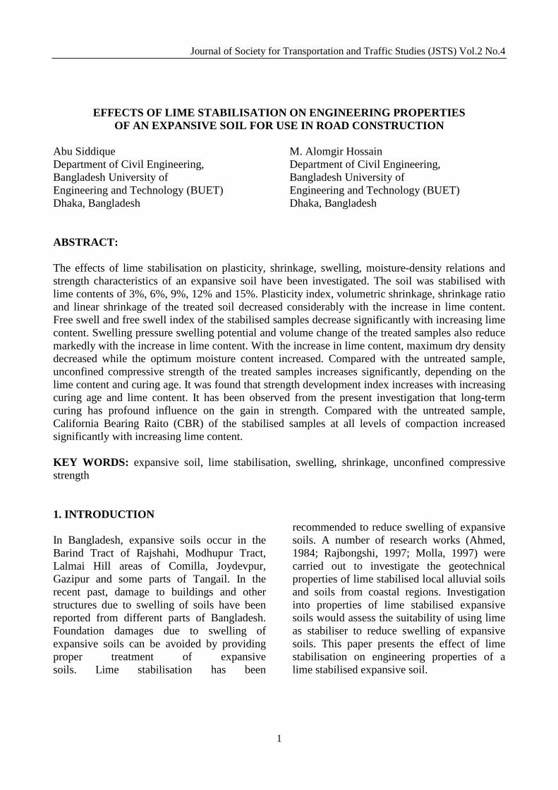
Abu Siddique M. Alomgir Hossain Department of Civil Engineering, Department of Civil Engineering, Bangladesh University of Bangladesh University of Engineering and Technology (BUET) Engineering and Technology (BUET) Dhaka, Bangladesh Dhaka, Bangladesh ABSTRACT: The effects of lime stabilisation on plasticity, shrinkage, swelling, moisture-density relations and strength characteristics of an expansive soil have been investigated. The soil was stabilised with lime contents of 3%, 6%, 9%, 12% and 15%. Plasticity index, volumetric shrinkage, shrinkage ratio and linear shrinkage of the treated soil decreased considerably with the increase in lime content. Free swell and free swell index of the stabilised samples decrease significantly with increasing lime content. Swelling pressure swelling potential and volume change of the treated samples also reduce markedly with the increase in lime content. With the increase in lime content, maximum dry density decreased while the optimum moisture content increased. Compared with the untreated sample, unconfined compressive strength of the treated samples increases significantly, depending on the lime content and curing age. It was found that strength development index increases with increasing curing age and lime content. It has been observed from the present investigation that long-term curing has profound influence on the gain in strength. Compared with the untreated sample, California Bearing Raito (CBR) of the stabilised samples at all levels of compaction increased significantly with increasing lime content. KEY WORDS: expansive soil, lime stabilisation, swelling, shrinkage, unconfined compressive strength
1. INTRODUCTION In Bangladesh, expansive soils occur in the Barind Tract of Rajshahi, Modhupur Tract, Lalmai Hill areas of Comilla, Joydevpur, Gazipur and some parts of Tangail. In the recent past, damage to buildings and other structures due to swelling of soils have been reported from different parts of Bangladesh. Foundation damages due to swelling of expansive soils can be avoided by providing proper treatment of expansive soils. Lime stabilisation has been
recommended to reduce swelling of expansive soils. A number of research works (Ahmed, 1984; Rajbongshi, 1997; Molla, 1997) were carried out to investigate the geotechnical properties of lime stabilised local alluvial soils and soils from coastal regions. Investigation into properties of lime stabilised expansive soils would assess the suitability of using lime as stabiliser to reduce swelling of expansive soils. This paper presents the effect of lime stabilisation on engineering properties of a lime stabilised expansive soil.

Journal of Society for Transportation and Traffic Studies (JSTS) Vol.2 No.4
2
2. SOIL USED AND LABORATORY TESTING PROGRAMME The expansive soil was collected from Rajendrapur Cantonment, Gajipur. Disturbed and undisturbed samples were collected from the site. Liquid limit, plasticity index, shrinkage limit and linear shrinkage of the soil were found to be 56%, 43, 11% and 20%, respectively. The soil is clay of high plasticity. Free swell, free swell index, swelling pressure, swelling potential and volume change from air-dry to saturated condition of the soil have been found to be 75%, 40%, 53 kN/m2, 1.8% and 29%, respectively. By comparing the laboratory measured values of index and swelling properties of the soil with the various recommended criteria of expansive soils, the overall degree of expansion of the soil has been found to be high. The following testing program was undertaken for the expansive soil: (i) Index properties, swelling properties and
moisture-density relations of the untreated soil and soil treated with five different lime contents of 3%, 6%, 9%, 12% and 15% were determined.
(ii) Unconfined compressive strength test on compacted cylindrical samples of 71 mm diameter by 142 mm high tests were carried out on untreated and treated soil Unconfined compressive strength tests were carried out on lime treated samples cured at different ages of 1 week, 2 weeks, 4 weeks, 8 weeks and 16 weeks.
(iii) California Bearing Ratio (CBR) tests were carried out on untreated soil and soil treated with five different lime contents of 3%, 6%, 9%, 12% and 15%. Hossain (2001) reported details of sample preparation, procedures for various tests and equipment.
3. TEST RESULTS AND DISCUSSIONS 3.1 Effect of lime stabilisation on plasticity and shrinkage characteristics The values of plasticity and shrinkage properties of the untreated and lime stabilised samples of the expansive soil are shown in Table 1. Compared with the untreated sample, the following effects of lime stabilisation on the plasticity and shrinkage properties of the soil were observed:
• Liquid limit of the stabilised samples initially decreased with the addition of lime content and then increased.
• Plastic limit and shrinkage limit increased significantly.
• Plasticity index, volumetric shrinkage, shrinkage ratio and linear shrinkage decreased markedly.
Plasticity indices of the treated samples were found to reduce by 30% to 56%. Ahmed (1984) found an increase in plastic limit while liquid limit and the plasticity index decreased with increasing addition of lime. Rajbongshi (1997) found an increase in plastic limit while liquid limit and the plasticity index reduced with increasing addition lime content. Holtz (1969) found that lime drastically reduces liquid limit and plasticity index of mont morillonitic clays. Compared with the untreated sample, shrinkage limit has been found to increase by 2 to 3.36 times while linear shrinkage was found to reduce by 35% to 75%. Rajbongshi (1997) also found an increase in shrinkage limit while linear shrinkage reduced with increasing addition of lime for samples of a coastal soil of Bangladesh. IRC (1976) and Bell (1993) also reported reduction in linear shrinkage with increasing lime content. Holtz (1969) found that lime drastically raises the shrinkage limit of expansive montmorillonitic clays. Compared with the untreated sample, volumetric shrinkage and shrinkage ratio were found to reduce by 48% to 82% and 31% to 46%, respectively, due to lime stabilisation.

Journal of Society for Transportation and Traffic Studies (JSTS) Vol.2 No.4
3
Table 1 Comparison of Index and Shrinkage Properties of Untreated and Lime Treated Expansive Soil Samples
Index and Shrinkage Properties Lime Content (%)
0 3 6 9 12 15 Liquid Limit (%) 56 54 53 54 57 59 Plastic Limit (%) 13 24 28 32 37 40 Plasticity Limit (%) 43 30 25 22 20 19 Shrinkage Limit (%) 11 22 25 29 33 37 Volumetric Shrinkage (%) 90 47 36 23 18 16 Shrinkage Ratio 2.02 1.39 1.30 1.20 1.15 1.10 Linear Shrinkage (%) 20 13 11 9 7 5 3.2 Effect of lime stabilisation on swelling properties Table 2 presents a comparison of the swelling properties of untreated and lime stabilised samples of the expansive soil. Table 2 shows the following effects of lime stabilisation on swelling properties:
• Free swell and free swell index of the stabilised samples decreased markedly. Compared with the untreated sample, free swell and fee swell index were found to reduce by 17% to 87% and 38% to 95%, respectively, due to stabilisation with 3% to 15% lime.
• Swelling pressure and swelling potential of the treated samples reduced considerably. Swelling pressure and swelling potential become zero when the
soil has been stabilised with 9% and 12% lime. These reduced swell characteristics are generally attributed to decreased affinity for water of the calcium saturated clay and the formation of a cementious matrix that resists volumetric expansion.
• Volume change of the stabilised samples from air-dry to saturated condition decreases significantly. Volume change of the stabilised samples from air-dry to saturated condition was found to decease by 55% to 83%.
The above mentioned results on the influence of lime stabilisation on swelling properties of the expansive soil clearly demonstrate that lime is an effective additive in reducing the various swelling properties of an expansive soil.
Table 2 Comparisons of Swelling Properties of Untreated and Lime Stabilised Samples
Swelling Properties Lime Content (%)
0 3 6 9 12 15 Free Swell (%) 75 62 52 38 15 10 Free Swell Index (%) 40 25 17 10 4 2 Swelling Pressure of Laboratory Compacted Sample (%)
53 15 7 2 0 0
Swelling Potential of Laboratory Compacted Sample (%)
1.8 0.40 0.20 0.075 0 0
Volume Change from Air-dry to Saturated Condition (%)
29.0 13.0 10.8 7.5 6.0 5.0

Journal of Society for Transportation and Traffic Studies (JSTS) Vol.2 No.4
4
3.3 Moisture-density relations of treated and untreated samples Moisture-density relations of untreated and lime treated samples of the soil are shown in Figure 1. From the relations presented in Figure1, the maximum dry density (γdmax) and optimum moisture content (wopt) of samples of the soil have been determined which are presented in Table 3. It can be seen from Table 3 that with the increase in lime content values of γdmax decreased while the values of wopt increased. It was found that compared with the untreated sample, the values of γdmax decreased by 10% to 17% for an increase in lime content from 3% to 15%. The values of wopt have been found to increase by 10% to
65% due to stabilisation with 3% to 15% lime. Ahmed (1984) found that for sandy silt and silty clay soils of Bangladesh, the maximum dry density reduced with the increase in lime content. Serajuddin and Azmal (1991) also found that compared with untreated samples the maximum dry density of lime treated samples of two fine-grained regional soils decreased while optimum moisture content slightly increased. For a Chittagong coastal soil, Rajbongshi (1997) reported an increase in wopt and a reduction in γdmax. Molla (1997) also found an increase in wopt and a reduction in γdmax for three regional soils (liquid limit = 34 to 47, plasticity index = 9 to 26) of Bangladesh stabilised with lime.
Figure 1 Moisture – density relations of untreated and lime treated samples of expansive soil

Journal of Society for Transportation and Traffic Studies (JSTS) Vol.2 No.4
5
Table 3 Values of Maximum Dry – density and Optimum Moisture Content of Untreated and Lime Treated Expansive Soil
Lime Content (%) γdmax (%) wopt (%)
0 17.08 18.10 3 15.34 19.90 6 15.08 23.80 9 14.75 25.60 12 14.44 27.70 15 14.10 29.90
3.4 Effect of lime stabilisation on unconfined compressive strength Table 4 shows a summary of the unconfined compression test results of the treated samples of the soil. Unconfined compressive strength of the untreated sample was found to be 550 kN/m2. Table 4 shows that compared with the untreated sample, the values of qu of the treated samples increased significantly, depending on the lime content and curing age. It has been observed from the present investigation that long-term curing (up to 16 weeks) has marked influence on the gain in strength. It has been found that at any particular lime content, unconfined compressive strength continued to increase with the increase in curing age. The effect of long-term curing on the increase in unconfined compressive strength was found to be more pronounced when samples were stabilised with higher lime contents (more than 3%). It was found that the value of qu of sample treated with 15% lime and cured at 16 weeks was about 8.4 times higher than the strength of the untreated sample. The relationship between qu for different lime contents and for samples cured at different ages is shown in Figure 2. Figure 2 shows that the values of qu of treated samples cured at any particular age increased with increasing lime content and that values of qu of samples treated with a particular lime content increased with the increase in curing age. Serajuddin and Azmal (1991) also reported that the unconfined compressive strength of regional alluvial soils of Bangladesh treated
with 5%, 7.5% and 10% slaked lime increased with the increase in lime content and curing age. Rajbongshi (1997) reported that unconfined compressive strength of lime treated samples increased with the increase in lime content and curing age for large diameter samples (71 m diameter by 142 mm high). Hasan (2002) also reported increase in unconfined compressive strength with increasing lime content for large diameter samples of silty clay collected from a reclaimed site of Dhaka city. Molla (1997) found that unconfined compressive strength of lime treated samples increased with the increase in lime content and curing age for three regional soils of Bangladesh. The rate of strength gain with curing time has been evaluated in terms of the parameter strength development index (SDI) as proposed by Uddin (1995) and defined as follows: SDI = (Strength of Stabilised sample - Strength of untreated sample) / Strength of untreated sample Plots of SDI versus curing age of treated samples are shown in Figure 3. Figure 3 shows that for samples stabilised with any particular lime content, the values of SDI increases with increasing curing age. Figure 3 also shows that for samples cured at any particular age, SDI increases with the increase in lime content. Figure 3 clearly shows that the relative degree of strength gain resulted due to increasing curing age and lime content. As can be seen from Figure 3 that long-term

Journal of Society for Transportation and Traffic Studies (JSTS) Vol.2 No.4
6
curing has got significant effect on strength development. Rajbongshi (1997) and Hasan (2002) also reported increase in SDI with
increasing curing time and lime content, as obtained in the present investigation.
Table 4 Unconfined Compressive Strength of Lime Stabilised Expansive Soil Samples
Cement Content (%) Unconfined Compressive Strength, qu (kN/m2) 1 week 2 weeks 4 weeks 8 weeks 16 weeks
3 750 850 1100 1230 1350 6 1010 1120 1820 2450 3100 9 1100 1220 1930 2640 3450 12 1180 1350 2300 2840 3980 15 1440 1620 2650 3150 4600
Figure 2 Effect of Lime Content on Unconfined Compressive strength
Figure 3 SDI versus Curing Curves for Lime Treated Expansive Soil
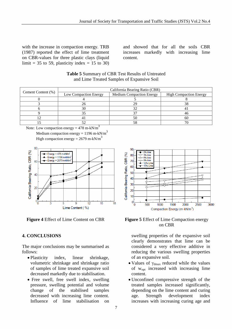
3.5 Effect of lime stabilisation on California Bearing Ratio (CBR) A summary of the CBR test result for samples of the expansive soil is presented in Table 5. In order to investigate CBR-dry density relationship for untreated and stabilised samples, CBR tests were performed on samples compacted using three levels of compaction energies, e.g., low compaction energy (478 m-kN/m3), medium compaction energy (1196 m-kN/m3) and high compaction energy (2679 m-kN/m3). It can be seen from Table 5 that compared with the untreated sample, CBR-values of the treated samples at all levels of compaction increased considerably. The variation of CBR with lime content is shown in Figure 4, while Figure 5 presents
the CBR versus compaction energy plots for the same samples. It can be seen from Figure 4 that at all levels of compaction, CBR increases markedly with increasing lime content while Figure 5 shows that at any particular lime content, CBR increases significantly with the increase in compaction energy. It has been found that compared with the untreated sample, CBR-values of treated samples increased by 4.75 to 8.75 times due to increase in lime content from 3% to 15%. Molla (1997) and Rajbongshi (1997) investigated the effect of lime on CBR-values of three regional soils and a coastal soil of Bangladesh, respectively. It was found that CBR value of stabilised samples increased with increasing lime content. Rajbongshi (1997) also reported that at any particular lime content, CBR increased significantly
Journal of Society for Transportation and Traffic Studies (JSTS) Vol.2 No.4
7
with the increase in compaction energy. TRB (1987) reported the effect of lime treatment on CBR-values for three plastic clays (liquid limit = 35 to 59, plasticity index = 15 to 30)
and showed that for all the soils CBR increases markedly with increasing lime content.
Table 5 Summary of CBR Test Results of Untreated
and Lime Treated Samples of Expansive Soil
Cement Content (%) California Bearing Ratio (CBR)
Low Compaction Energy Medium Compaction Energy High Compaction Energy 0 4 5 8 3 26 29 38 6 30 32 41 9 35 37 46 12 41 50 60 15 52 58 70
Note: Low compaction energy = 478 m-kN/m3 Medium compaction energy = 1196 m-kN/m3 High compaction energy = 2679 m-kN/m3
Figure 4 Effect of Lime Content on CBR
Figure 5 Effect of Lime Compaction energy
on CBR 4. CONCLUSIONS The major conclusions may be summarised as follows:
• Plasticity index, linear shrinkage, volumetric shrinkage and shrinkage ratio of samples of lime treated expansive soil decreased markedly due to stabilisation.
• Free swell, free swell index, swelling pressure, swelling potential and volume change of the stabilised samples decreased with increasing lime content. Influence of lime stabilisation on
swelling properties of the expansive soil clearly demonstrates that lime can be considered a very effective additive in reducing the various swelling properties of an expansive soil.
• Values of γdmax reduced while the values of wopt increased with increasing lime content.
• Unconfined compressive strength of the treated samples increased significantly, depending on the lime content and curing age. Strength development index increases with increasing curing age and

Journal of Society for Transportation and Traffic Studies (JSTS) Vol.2 No.4
8
increasing lime content. Long-term curing has marked influence on the gain in strength.
• CBR-values of the treated samples increased considerably with increasing lime content. At any particular lime content, CBR increased significantly with the increase in compaction energy.

Journal of Society for Transportation and Traffic Studies (JSTS) Vol.2 No.4
9
REFERENCES Ahmed, N.U. (1984). Geotechnical properties of selected local soils stabilised with lime and cement, M.Sc. Engineering Thesis, Department of Civil Engineering, BUET, Dhaka, Bangladesh. Bell, F.G. (1993). Engineering treatment of Soils, E & FN Spon, An Imprint of Chapman & Hall, First Edition, London, U.K. Hasan, K. A. (2002). A study of cement and lime stabilisation on soils of selected reclaimed sites of Dhaka city, M. Sc. Engineering thesis, Department of Civil Engineering, BUET, Dhaka, Bangladesh. Hossain, M. A. (2001). Geotechnical behaviour of a lime treated expansive soil, M. Sc. Engineering thesis, Department of Civil Engineering, BUET, Dhaka, Bangladesh. Holtz, W.G. (1969). Volume change in expansive clay soils and control by lime treatment, Proc., Second International Research and Engineering Conference on Expansive Soils, Texax A& M Press. IRC (Indian Road Congress) (1976). State-of-the-Art: Lime-soil stabilisation, Special Report, IRC Highway Research Board, New Delhi. Molla, M.A.A. (1997). Effect of compaction conditions and state variables on engineering properties of the lime stabilised soil, M.Sc. Engineering Thesis, Department of Civil Engineering, BUET, Dhaka. Rajbongshi, B. (1997). A study on cement and lime stabilised Chittagong coastal soils for use in road construction, M.Sc. Engineering Thesis, Department of Civil Engineering, BUET, Dhaka. Serajuddin, M. and Azmal, M. (1991). Fine-grained soils of bangladesh for road construction, Proc., 9th ARC on Soil Mechanics and Foundation Engineering, Vol. 1, Bangkok, Thailand, 175-178. TRB (Transportation Research Board) (1987). State-of-the-Art report: Lime stabilisation research, Proeprties, Design, and Construction", National Research Council, Washington, D.C. Uddin, M.K. (1995). Strength and deformation characteristics of cement-treated Bangkok clay, Ph.D. Thesis, Asian Institute of Technology, Bangkok, Thailand.

Journal of Society for Transportation and Traffic Studies (JSTS) Vol.2 No.4
10
THE STUDY ON TRIP GENERATION MODEL OF RESIDENTIAL B UILDING IN BANGKOK AREA
Chisanu AMPRAYN Assistant dean in student affairs Department of Civil Engineering, Faculty of Engineering Sripatum University 61 Phahonyothin Road Chatuchak District Bangkok 10900 Fax: +6625791111 ext 2147 E-mail: [email protected]
Vatanavongs RATANAVARAHA Associate Professor Department of Transportation Engineering Suranaree University of Technology 111 Mahavitayalai Road, Amphur Muang Nakhonratchasima 30000 Fax: +6644224608 E-mail: [email protected]
ABSTRACT: There has been blooming development in high density residential building in Bangkok and its surrounding area. Such residential buildings generate a lot of traffic volume additional to the existing demand on the road network. This study tries to estimate number of vehicle trip ends depending on weekday and weekend behavior. Multiple regression analysis with stepwise method was applied to develop the relationship between vehicle trip ends and each independent variable. In weekday behavior, there were four potential independent variables including number of residential unit (X2), total recreational area (X7), the number of route of directly passing public bus/van (X9), and number of entrance and exit point (X12) in each sample. In contrast, in weekend behavior, there were five potential independent variables which were X2, unit price (X4), X9, the distance between each sample and main road (X10), and X12. Better estimating trip generation is recommended for a reduction of the traffic impact surrounding the residential building. Consequently, more efficient and safer travelling of residents can be achieved. KEY WORDS: Trip ends, Dependent Variable, Independent Variable 1. INTRODUCTION Recently, high density residential building industry has been massively developed in Bangkok and its suburbs. Such buildings generate a number of subsequent trips which cause problematic transportation network especially at the bottle neck area such as an entrance and an exit. Thus, an estimation of the number of trips is very important for traffic management. The proposed trip generation on new residential buildings is meaningful when precised values are obtained. Trip generation analysis is a proper alternative to estimate number of trip ends, which can separate into two groups as weekday and weekend character. Therefore,
transportation planners are able to use number of trip ends in order to express the mitigation measures, which compatible with real time traffic condition and their network. 2. SAMPLE SELECTION AND DATA COLLECTION A selection of sample residential buildings in this study is based on following factors:
• A distance between the building and main street is less than 200 meters or within a walking distance. Residents can easily access to major public transport systems.
• A unit per building is more than 500 units
Journal of Society for Transportation and Traffic Studies (JSTS) Vol.2 No.4
11
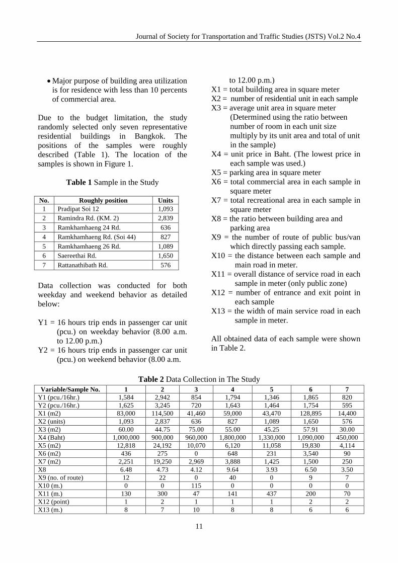
• Major purpose of building area utilization is for residence with less than 10 percents of commercial area.
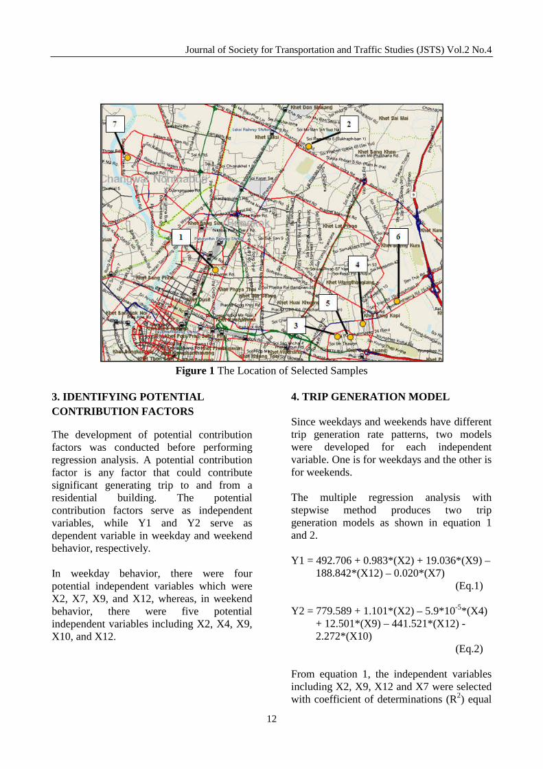
Due to the budget limitation, the study randomly selected only seven representative residential buildings in Bangkok. The positions of the samples were roughly described (Table 1). The location of the samples is shown in Figure 1.
Table 1 Sample in the Study
No. Roughly position Units 1 Pradipat Soi 12 1,093 2 Ramindra Rd. (KM. 2) 2,839
3 Ramkhamhaeng 24 Rd. 636
4 Ramkhamhaeng Rd. (Soi 44) 827
5 Ramkhamhaeng 26 Rd. 1,089 6 Saereethai Rd. 1,650
7 Rattanathibath Rd. 576
Data collection was conducted for both weekday and weekend behavior as detailed below: Y1 = 16 hours trip ends in passenger car unit
(pcu.) on weekday behavior (8.00 a.m. to 12.00 p.m.)
Y2 = 16 hours trip ends in passenger car unit (pcu.) on weekend behavior (8.00 a.m.
to 12.00 p.m.) X1 = total building area in square meter X2 = number of residential unit in each sample X3 = average unit area in square meter
(Determined using the ratio between number of room in each unit size multiply by its unit area and total of unit in the sample)
X4 = unit price in Baht. (The lowest price in each sample was used.)
X5 = parking area in square meter X6 = total commercial area in each sample in
square meter X7 = total recreational area in each sample in
square meter X8 = the ratio between building area and
parking area X9 = the number of route of public bus/van
which directly passing each sample. X10 = the distance between each sample and
main road in meter. X11 = overall distance of service road in each
sample in meter (only public zone) X12 = number of entrance and exit point in
each sample X13 = the width of main service road in each
sample in meter. All obtained data of each sample were shown in Table 2.
Table 2 Data Collection in The Study Variable/Sample No. 1 2 3 4 5 6 7
Y1 (pcu./16hr.) 1,584 2,942 854 1,794 1,346 1,865 820 Y2 (pcu./16hr.) 1,625 3,245 720 1,643 1,464 1,754 595 X1 (m2) 83,000 114,500 41,460 59,000 43,470 128,895 14,400 X2 (units) 1,093 2,837 636 827 1,089 1,650 576 X3 (m2) 60.00 44.75 75.00 55.00 45.25 57.91 30.00 X4 (Baht) 1,000,000 900,000 960,000 1,800,000 1,330,000 1,090,000 450,000 X5 (m2) 12,818 24,192 10,070 6,120 11,058 19,830 4,114 X6 (m2) 436 275 0 648 231 3,540 90 X7 (m2) 2,251 19,250 2,969 3,888 1,425 1,500 250 X8 6.48 4.73 4.12 9.64 3.93 6.50 3.50 X9 (no. of route) 12 22 0 40 0 9 7 X10 (m.) 0 0 115 0 0 0 0 X11 (m.) 130 300 47 141 437 200 70 X12 (point) 1 2 1 1 1 2 2 X13 (m.) 8 7 10 8 8 6 6
Journal of Society for Transportation and Traffic Studies (JSTS) Vol.2 No.4
12
Figure 1 The Location of Selected Samples
3. IDENTIFYING POTENTIAL CONTRIBUTION FACTORS
The development of potential contribution factors was conducted before performing regression analysis. A potential contribution factor is any factor that could contribute significant generating trip to and from a residential building. The potential contribution factors serve as independent variables, while Y1 and Y2 serve as dependent variable in weekday and weekend behavior, respectively. In weekday behavior, there were four potential independent variables which were X2, X7, X9, and X12, whereas, in weekend behavior, there were five potential independent variables including X2, X4, X9, X10, and X12.
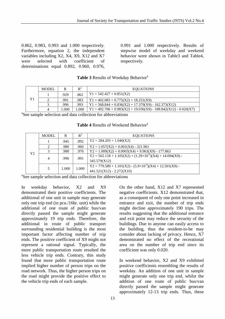
4. TRIP GENERATION MODEL Since weekdays and weekends have different trip generation rate patterns, two models were developed for each independent variable. One is for weekdays and the other is for weekends. The multiple regression analysis with stepwise method produces two trip generation models as shown in equation 1 and 2. Y1 = 492.706 + 0.983*(X2) + 19.036*(X9) – 188.842*(X12) – 0.020*(X7) (Eq.1) Y2 = 779.589 + 1.101*(X2) – 5.9*10-5*(X4) + 12.501*(X9) – 441.521*(X12) - 2.272*(X10) (Eq.2) From equation 1, the independent variables including X2, X9, X12 and X7 were selected with coefficient of determinations (R2) equal
Journal of Society for Transportation and Traffic Studies (JSTS) Vol.2 No.4
13
0.862, 0.983, 0.993 and 1.000 respectively. Furthermore, equation 2, the independent variables including X2, X4, X9, X12 and X7 were selected with coefficient of determinations equal 0.892, 0.960, 0.976,
0.991 and 1.000 respectively. Results of stepwise model of weekday and weekend behavior were shown in Table3 and Table4, respectively.
Table 3 Results of Weekday Behaviora
Y1
MODEL R R2 EQUATIONS
1 .929 .862 Y1 = 542.427 + 0.851(X2)
2 .991 .983 Y1 = 402.083 + 0.775(X2) + 18.251(X9) 3 .996 .993 Y1 = 568.844 + 0.836(X2) + 17.379(X9) - 162.373(X12) 4 1.000 1.000 Y1 = 492.706 + 0.983(X2) + 19.036(X9) - 188.842(X12) - 0.020(X7)
aSee sample selection and data collection for abbreviations
Table 4 Results of Weekend Behaviora
Y2
MODEL R R2 EQUATIONS
1 .945 .892 Y2 = 284.203 + 1.040(X2)
2 .980 .960 Y2 = 1.057(X2) + 0.001(X4) - 321.961 3 .988 .976 Y2 = 1.009(X2) + 0.0003(X4) + 9.963(X9) - 177.863
4 .996 .991 Y2 = 502.118 + 1.105(X2) + (1.29×10⁻⁵)(X4) + 14.094(X9) - 345.579(X12)
5 1.000 1.000 Y2 = 779.589 + 1.101(X2) - (5.9×10⁻⁵)(X4) + 12.501(X9) - 441.521(X12) - 2.272(X10)
aSee sample selection and data collection for abbreviations In weekday behavior, X2 and X9 demonstrated their positive coefficients. The additional of one unit in sample may generate only one trip end (in pcu./16hr. unit) while the additional of one route of public bus/van directly passed the sample might generate approximately 19 trip ends. Therefore, the additional in route of public transport surrounding residential building is the most important factor affecting number of trip ends. The positive coefficient of X9 might not represent a rational signal. Typically, the more public transportation route resulted the less vehicle trip ends. Contrary, this study found that more public transportation route implied higher number of person trips on the road network. Thus, the higher person trips on the road might provide the positive effect to the vehicle trip ends of each sample.
On the other hand, X12 and X7 represented negative coefficients. X12 demonstrated that, as a consequent of only one point increased in entrance and exit, the number of trip ends might decline approximately 190 trips. The results suggesting that the additional entrance and exit point may reduce the security of the buildings. Due to anyone can easily access to the building, thus the resident-to-be may consider about lacking of privacy. Hence, X7 demonstrated no effect of the recreational area on the number of trip end since its coefficient was only 0.020. In weekend behavior, X2 and X9 exhibited positive coefficients resembling the results of weekday. An addition of one unit in sample might generate only one trip end, whilst the addition of one route of public bus/van directly passed the sample might generate approximately 12-13 trip ends. Thus, these

Journal of Society for Transportation and Traffic Studies (JSTS) Vol.2 No.4
14
can be assumed that increased bus/van route provided stronger impact on the trip end of weekday. Contrary, X4, X12, and X10 depicted negative coefficients. Only X12 showed similar result to the weekday behavior with greater impact. The only one entrance and exit increase, the number of trip ends were reduced 440 trips. The futures residents may strongly consider in relax lifestyle and privacy, so passing by strangers are undesired. When the additional unit price (X4) was 100,000 baht per unit, trip ends were reduced approximately six trips. The higher price of building unit implies the more coziness for the future residents. Coziness in the residence is important as the residents would love to be at home rather than going out for any purpose. At last, X10 was only one variable illustrated negative coefficient. One meter increased of the distance between residential buildings to main road affected the declined number of trip ends for approximately 2 trips. This is because everyone spent their time at home during weekends, thus less travels were generated.
5. CONCLUSIONS The study developed trip generation model on residential building by using stepwise method. The models include weekday and weekend characteristics. The conclusions of the study are as follows:
• Number of unit (X2) and number of route of bus/van directly passing the sample (X9) are two main factors in order to give the positive value of trip ends in both weekday and weekend behavior.
• Number of entrance and exit point (X12) is the one factor that decrease the number of trip ends in both weekday and weekend behavior. X12 is the most important factor to decrease number of trip ends in the study
• Unit price (X4) and distance between sample and main road (X10) are two factors that decrease number of trip ends in weekend behavior only.
6. RECOMMENDATIONS Due to budget limitation, the study randomly selected only seven samples in order to find out the trip generation model. To produce the trip generation model more precisely, the number of sample must be added

Journal of Society for Transportation and Traffic Studies (JSTS) Vol.2 No.4
15
REFERENCES
Higuchi, Y (1995) Lectures on Multivariate Analysis for Human Settlements Planning. Department of Mechanical and Environmental Informatics, Graduate School of Information Science and Engineering, Tokyo Institute of Technology. Ratanavaraha V. and Ampray C. (2005). A Predictive Trip Generation Model for Hypermarkets in Bangkok, Proceeding of the 4th Asia Pacific Conference on Transportation and Environment, Xi’An, China.

Journal of Society for Transportation and Traffic Studies (JSTS) Vol.2 No.4
16
ANALYSIS OF DRIVING CONDITIONS AND PREFERRED MEDIA ON DIVERSION
Yoonhyuk CHOI Associate Researcher, Ph.D. Transportation Research Division Korea Expressway Corporation Research Institute 50-5, Sancheok-ri, Dongtan-myeon, Hwaseong- Si, Gyeonggi-Do, Republic of Korea Fax: +82-31-371-3319 E-mail: [email protected] ABSTRACT: Studies on the distribution of traffic demands have been proceeding by providing traffic information for reducing greenhouse gases and reinforcing the road's competitiveness in the transport section, however, since it is preferentially required the extensive studies on the driver's behavior changing routes and its influence factors, this study has been developed a discriminant model for changing routes considering driving conditions including traffic conditions of roads and driver's preferences for information media. It is divided into three groups depending on driving conditions in group classification with the CART analysis, which is statistically meaningful. And the extent that driving conditions and preferred media affect a route change is examined through a discriminant analysis, and it is developed a discriminant model equation to predict a route change. As a result of building the discriminant model equation, it is shown that driving conditions affect a route change much more, the entire discriminant hit ratio is derived as 64.2%, and this discriminant equation shows high discriminant ability more than a certain degree. KEY WORDS: Diversion, Driving conditions, Preferred media, Discrimint model, CART analysis 1. INTRODUCTION 1.1 Backgrounds and Purposes Interests in the greenhouse gas reduction and the environmental friendly green growth are increasing as the global warming problems are aggravated. It is more and more interested in how to efficiently use the existing roads in order to reduce greenhouse gases and reinforce road's competitiveness in the transport section, and studies on the distribution of traffic demands by providing traffic information are in progress as a practical method for them. However, driver's decision making to change routes is not a problem whether or not the information is simply provided, but may be varied depending on driving conditions or preferred
media when it is provided. In other words, driver's responses for route changes may be varied depending on the driving conditions such as weather situations and traveling distances etc. and the individual driver's preferred property for media to provide information even though the same information is provided. In particular, even though a result of driver's decision making to change routes is represented as a simple result whether to drive the existing route or change the route, the process to actually determine it is carried out through a diverse, complex and step by-step process such as examining various environmental conditions, considering the worst situation, and ranking priority in accordance with the preferred property for each person. Therefore, it is needed a study
Journal of Society for Transportation and Traffic Studies (JSTS) Vol.2 No.4
17
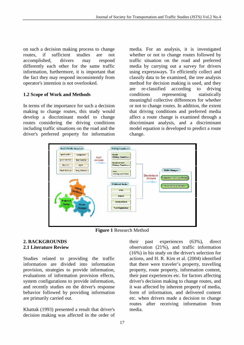
on such a decision making process to change routes, if sufficient studies are not accomplished, drivers may respond differently each other for the same traffic information, furthermore, it is important that the fact they may respond inconsistently from operator's intention is not overlooked. 1.2 Scope of Work and Methods In terms of the importance for such a decision making to change routes, this study would develop a discriminant model to change routes considering the driving conditions including traffic situations on the road and the driver's preferred property for information
media. For an analysis, it is investigated whether or not to change routes followed by traffic situation on the road and preferred media by carrying out a survey for drivers using expressways. To efficiently collect and classify data to be examined, the tree analysis method for decision making is used, and they are re-classified according to driving conditions representing statistically meaningful collective differences for whether or not to change routes. In addition, the extent that driving conditions and preferred media affect a route change is examined through a discriminant analysis, and a discriminant model equation is developed to predict a route change.
Figure 1 Research Method
2. BACKGROUNDS 2.1 Literature Review Studies related to providing the traffic information are divided into information provision, strategies to provide information, evaluations of information provision effects, system configurations to provide information, and recently studies on the driver's response behavior followed by providing information are primarily carried out. Khattak (1993) presented a result that driver's decision making was affected in the order of
their past experiences (63%), direct observation (21%), and traffic information (16%) in his study on the driver's selection for actions, and H. R. Kim et al. (2004) identified that there were traveler’s property, travelling property, route property, information content, their past experiences etc. for factors affecting driver's decision making to change routes, and it was affected by inherent property of media, form of information, and delivered content etc. when drivers made a decision to change routes after receiving information from media.

Journal of Society for Transportation and Traffic Studies (JSTS) Vol.2 No.4
18
Y. H. Choi et al. (2007) identified in their study on the information media affecting driver's decision making to change routes that drivers depended on traffic information more than their own experiences as the congestion was more serious, and I. P. Kim (2008) found a primary factor deciding a detour through a preference analysis, and identified that a strategy was needed to provide each traffic information for each traffic situation that was a core factor of route changes. Meanwhile, Khattak et al. (2008) presented that media such as Internet, radio broadcasting, VMS, navigation etc. among information provision media affecting driver's behavior had affected the decision making of destinations, travelling means, route selections etc. In particular, when comparing the existing study's result of Khattak (1993, 2008), it could be found that individual driver's experiences were regarded as important in the 1990s, but preference for information media has been increasing more than personal experiences since the high reliable traffic information is timely provided via various media due to development of information communication technologies from the 2000s. Nevertheless, a remarkable fact is that even now, there are drivers who select routes using the past experiences in spite of the information age, and it is not irrelevant to user experiences (Ux) becoming an issue recently. The Ux means overall experiences that users feel and think as they directly or indirectly use any system, product, and service. It is a valuable experience that users could know by participating, using, observing, and interacting in every whole perceivable aspect as well as satisfaction on functions or procedures simply. Referring to the results of Khattak (1993) and Y. H. Choi et al. (2007), it is seemed that the past experiences such as user's direct driving experiences and indirect travelling experiences by persons around them affect a route selection primarily in the traffic aspect. Y. H. Choi et al. (2009) identified that there was a meaningful relationship between
driver's detour behaviors and road's traffic situations through a correlation analysis between the bypass rate investigated actually and the road's traffic situation (traffic volumes on the main line, travelling speed, and travelling time), and derived a regression equation for the expressway's bypass rate by using it. In addition, Y. H. Choi et al. (2010) analyzed how the use pattern of information media was varied according to traffic situations, and re-classified into passive use media, active use media, the past experiences based on the property for each medium to analyze variation of the bypass use rate for each information medium followed by each traffic situation. They identified that while the use rate of a passive use medium was decreased as the traffic situation became worse; the bypass rate using an active use medium and the past experiences was increased. S. N. Son (2010) identified that a will to change routes and driver's perceived behavior control for a route change most significantly affected a decision whether or not to change routes. 2.2 Problem statement In spite of many studies related to traffic information like this, studies on the driver's decision making to change routes are insufficient. In particular, since it has been identified that driver's route changes depend on traffic situations and the traffic information media used for changing routes become different according to traffic situations, an analysis on the relationship between traffic situations, preferred media, and route changes is needed by integrating them. This study is a succeeding study of Y. H. Choi et al. (2009, 2010), which would comprehensively analyze driver's property to change routes considered fragmentarily such as traffic situations and route changes, traffic situations and properties to use traffic information media etc. according to the property of preferred media under driving conditions such as travelling distances

Journal of Society for Transportation and Traffic Studies (JSTS) Vol.2 No.4
19
including road's traffic situations and weather conditions etc.
3. ANALYSIS METHODS This study performed an analysis with the following process.
Figure 2 Analysis Method First, it is performed whether or not to change routes for variables to be used in this study, definitions of the classification for road's traffic conditions and preferred media, and a fundamental statistical analysis. Second, for the appropriate classification of road's traffic situations which is a core part of this study, the CART analysis method is used to investigate road's traffic situations representing statistical meaningful collective differences for route changes. Third, a statistical verification is performed for the group classification of driving conditions by performing the one-way ANOVA for driving conditions classified by the CART analysis. Fourth, a discriminant model is developed for driving conditions and preferred media affecting the route changes.
Fifth, the discriminant hit ratio is analyzed for the developed discriminant analysis model. 4. DATA ANALYSIS 4.1 Fundamental Analysis This study performed a survey for total 500 persons using metropolitan expressways. Among total 500 of respondents, males occupied 60% as 286, and females occupied 40% as 214. In the result of responses having multiple choices asking whether or not to change routes for 8 road's traffic situations and 4 preferred media, the analysis was performed by using 6,462 data that the preference for each medium was responded above 8 points. It was because drivers having a preference of 'above favor' for the preferred media in each road's traffic situation were considered to represent well the relationship between the
Journal of Society for Transportation and Traffic Studies (JSTS) Vol.2 No.4
20
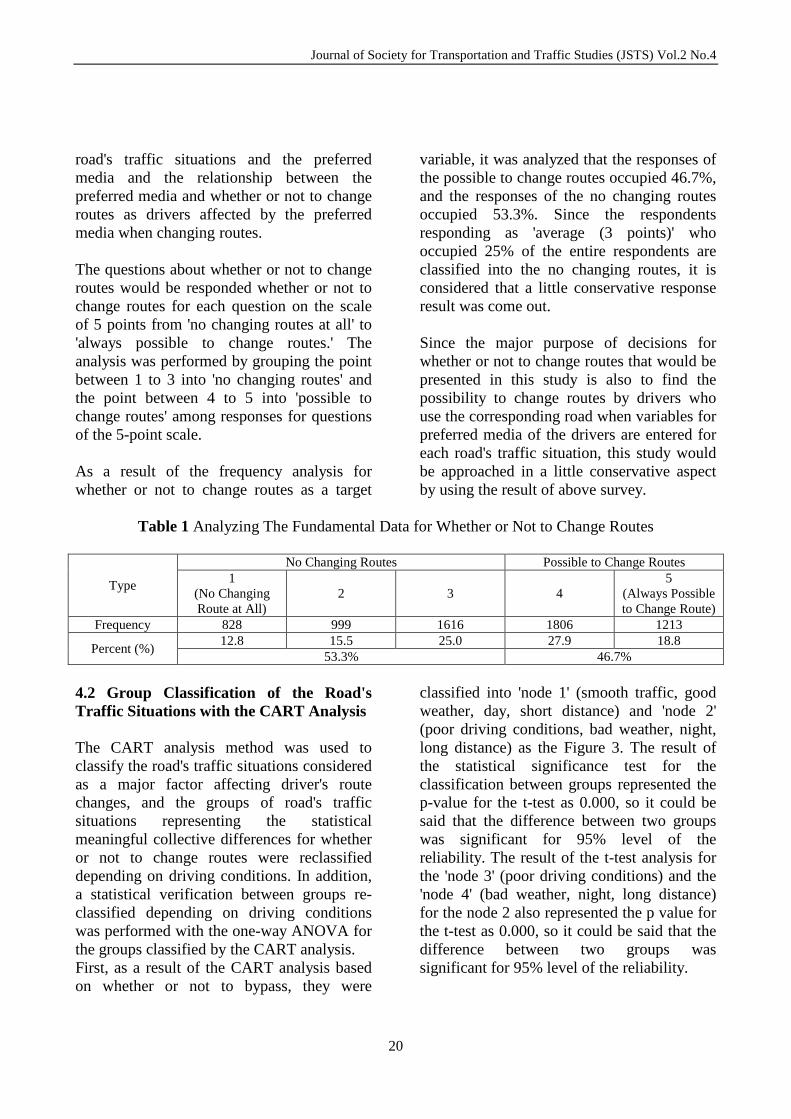
road's traffic situations and the preferred media and the relationship between the preferred media and whether or not to change routes as drivers affected by the preferred media when changing routes. The questions about whether or not to change routes would be responded whether or not to change routes for each question on the scale of 5 points from 'no changing routes at all' to 'always possible to change routes.' The analysis was performed by grouping the point between 1 to 3 into 'no changing routes' and the point between 4 to 5 into 'possible to change routes' among responses for questions of the 5-point scale. As a result of the frequency analysis for whether or not to change routes as a target
variable, it was analyzed that the responses of the possible to change routes occupied 46.7%, and the responses of the no changing routes occupied 53.3%. Since the respondents responding as 'average (3 points)' who occupied 25% of the entire respondents are classified into the no changing routes, it is considered that a little conservative response result was come out. Since the major purpose of decisions for whether or not to change routes that would be presented in this study is also to find the possibility to change routes by drivers who use the corresponding road when variables for preferred media of the drivers are entered for each road's traffic situation, this study would be approached in a little conservative aspect by using the result of above survey.
Table 1 Analyzing The Fundamental Data for Whether or Not to Change Routes
Type
No Changing Routes Possible to Change Routes 1
(No Changing Route at All)
2 3 4 5
(Always Possible to Change Route)
Frequency 828 999 1616 1806 1213
Percent (%) 12.8 15.5 25.0 27.9 18.8
53.3% 46.7%
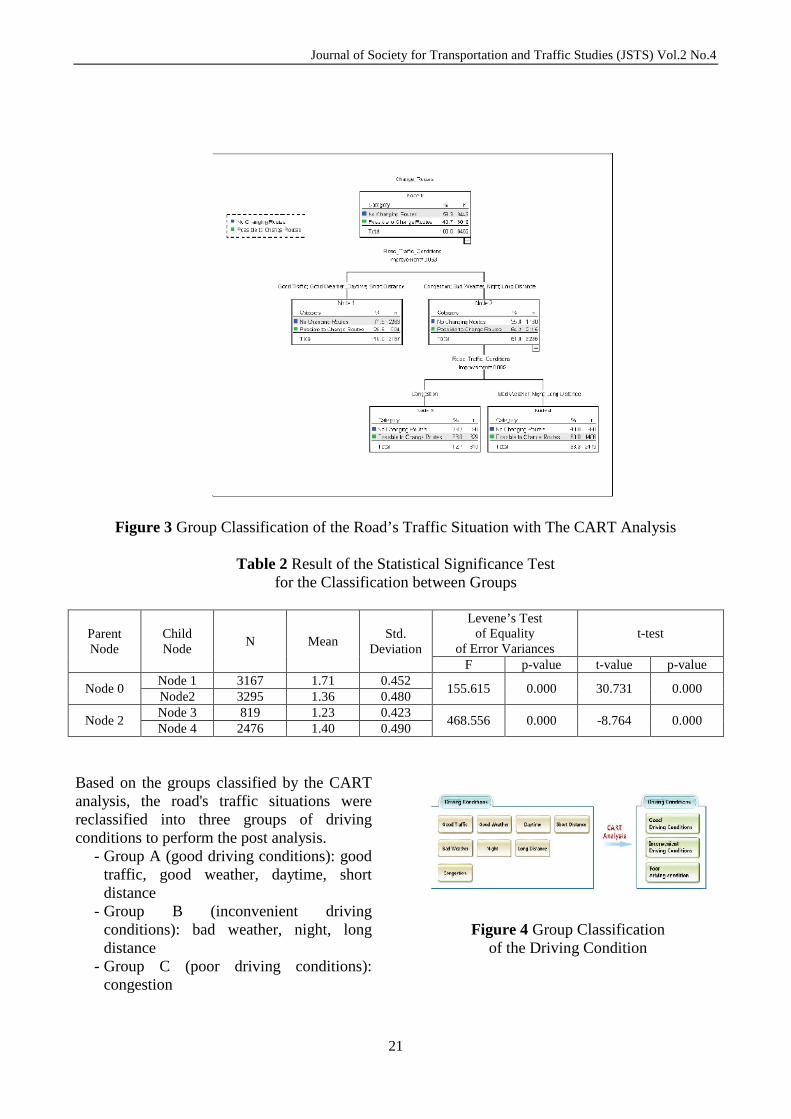
4.2 Group Classification of the Road's Traffic Situations with the CART Analysis The CART analysis method was used to classify the road's traffic situations considered as a major factor affecting driver's route changes, and the groups of road's traffic situations representing the statistical meaningful collective differences for whether or not to change routes were reclassified depending on driving conditions. In addition, a statistical verification between groups re-classified depending on driving conditions was performed with the one-way ANOVA for the groups classified by the CART analysis. First, as a result of the CART analysis based on whether or not to bypass, they were
classified into 'node 1' (smooth traffic, good weather, day, short distance) and 'node 2' (poor driving conditions, bad weather, night, long distance) as the Figure 3. The result of the statistical significance test for the classification between groups represented the p-value for the t-test as 0.000, so it could be said that the difference between two groups was significant for 95% level of the reliability. The result of the t-test analysis for the 'node 3' (poor driving conditions) and the 'node 4' (bad weather, night, long distance) for the node 2 also represented the p value for the t-test as 0.000, so it could be said that the difference between two groups was significant for 95% level of the reliability.
Journal of Society for Transportation and Traffic Studies (JSTS) Vol.2 No.4
21
Figure 3 Group Classification of the Road’s Traffic Situation with The CART Analysis
Table 2 Result of the Statistical Significance Test
for the Classification between Groups
Parent Node
Child Node
N Mean Std.
Deviation
Levene’s Test of Equality
of Error Variances t-test
F p-value t-value p-value
Node 0 Node 1 3167 1.71 0.452
155.615 0.000 30.731 0.000 Node2 3295 1.36 0.480
Node 2 Node 3 819 1.23 0.423
468.556 0.000 -8.764 0.000 Node 4 2476 1.40 0.490
Based on the groups classified by the CART analysis, the road's traffic situations were reclassified into three groups of driving conditions to perform the post analysis.
- Group A (good driving conditions): good traffic, good weather, daytime, short distance
- Group B (inconvenient driving conditions): bad weather, night, long distance
- Group C (poor driving conditions): congestion
Figure 4 Group Classification
of the Driving Condition

Journal of Society for Transportation and Traffic Studies (JSTS) Vol.2 No.4
22
The result of the one-way ANOVA and the post analysis to verify the difference between three groups classified by the driving condition represented the p-value as 0.000, and the difference between groups depending on the driving condition was the same as the CART analysis, so it had been proved that the group classification with the CART analysis was statistically appropriate. 4.3 Development of a Discriminar Model for Changing Routes 4.3.1 Outline The "1" of nominal scale was assigned to drivers changing routes, and the "0" of nominal scale was assigned to drivers not changing routes depending on whether or not to change routes for drivers using their own preferred media for each driving condition. The analysis with the stepwise method was
performed to understand variables affecting the route changes significantly, and the Wilks' method was used as the criteria to select variables. 4.3.2 Consideration of the Discriminant Analysis's Result (1) Analysis of Covariance Matrix The discriminant analysis is established under the assumption. It has a multi-variate normal distribution and the covariance of each group is identical. The homogeneity test result of the covariance matrix analyzed through the Box test for groups represented the significance probability of the Box test as 0.139, and it was selected the null hypothesis that their covariance are identical, so it could be defined that the covariance matrixes of two groups are identical.
Table 3 Result of the One-way ANOVA for Each Driving Condition
Driving Condition Mean Std. Deviation
Levene’s Test of Equality
of Error Variance One-Way ANOVA Post Hoc
Tests F-value Sig. F-value Sig.
Good Driving Conditions (a)
2.71 1.167
139.251 0.000 2337.863 0.000 a ≠ b ≠ c (Scheffe
Test)
Inconvenient Driving Conditions (b)
3.65 1.168
Poor Driving Condition (c)
4.12 0.910
Table 4 Summarizing the Introduced Variables of the Discriminant Model
Dependent Variable Independent Variable
Whether or Not to Change Routes
Driving Conditions (a) Good Driving Conditions (a1)
Inconvenient Driving Conditions (a2) Poor Driving Conditions (a3)
Preferred Media (b)
VMS (b1) Radio (b2)
Navigation (b3) Past Experience (b4)

Journal of Society for Transportation and Traffic Studies (JSTS) Vol.2 No.4
23
Table 5 Box’s Test Results
(2) Significance Test of the Discriminant Model As a result of the discriminant analysis, a discriminant function was derived, and it was analyzed that both the driving conditions and the preferred media had the statistically significant effects. Even though this analysis represented the canonical correlation coefficient as 0.310, the Eigenvalue as 0.107, the Wilks' lambda value as 0.904, which the discriminant were not very high, but the significant probability of the chi square test was 0.000 < =0.05, which represented that it was statistically significant. Examining the Wilks' lambda for road's traffic situations and preferred media and the value converting it into the F statistics also in the analysis on the discriminant factors, since the significant probability of the F statistics was less than 0.05, it could be said that the average difference of the discriminant score between groups was significant. The size of coefficient's absolute value in a discriminant equation represents the relative importance between variables, and it could be found that the driving conditions have more effects than the preferred media when it was examined the result analyzing the coefficients of the standardized canonical discriminant function for these discriminant factors.
Table 6 Summary of Canonical Discriminant Functions
Table 7 Standardized Canonical Discriminant Function Coefficients
Variable
Function Standardized
Canonical
Discriminant Function
Coefficients
Canonical
Discriminant Function
Coefficients Driving
Conditions 1.002 1.132
Preferred Media -0.239 -0.216 (Constant) - -1.635
(3) Establishment of the Standardized Canonical Discriminant Model The discriminant model equation was defined for whether or not to change routes by using the coefficients of the canonical discriminant function (non-standardized canonical discriminant function). Z = -1.635 + 1.132 x XFi – 0.216 x XMj (Eq.1) Here, Z: Whether or not to change routes
Box’s M 122.830 F Approx. 1.831
df 1 3 df 2 1.64710 Sig. 0.139
Eigen Values
Eigen Values
% of Varianc
e
Cumulative %
Cano- nical
Correlation
0.107 100.0 100.0 0.310
Wilks’ Lambda
Wilks’ Lambda
Chi Square
df Sig.
0.904 653.97 2 0.000 Test of
Equalityof
Group Means
Type Wilks’ F Sig.
Driving Conditions
0.909 649.788 0.000
Preferred Media
0.999 8.727 0.003

Journal of Society for Transportation and Traffic Studies (JSTS) Vol.2 No.4
24
XFi: Driving Condition (i: 1 = Good Driving Conditions, 2 = Inconvenient Driving Conditions, 3 = Poor Driving Conditions) XMj: Preferred Media (j: 1 = VMS, 2 = Radio, 3 = Navigation, 4 = Past Experience) If the discriminant score found by the above discriminant equation is larger than the classification standard, it is classified into the group 1 (possible to change routes), or if it is smaller, it is classified into the group 2 (no changing routes.) The average discriminant score of the group 1 is 0.349, and the average discriminant score of the group 2 is -0.306, which the standard of classification is calculated as the average of the cutting point of these two groups.
(Eq.2) Here; ni: Sample size of group i Ci: Centroid of group i The standard of classification is derived as the 0 of cutting point according to the above equation. Therefore, the case of having a larger value than the 0 by the discriminant model is classified into the group 1 (possible to change routes,) or if the value is less than the 0, it is classified into the group 2 (no changing routes.)
Table 8 Function at group Centroid
Changing Route Function 1
Centroid Cutting Point Possible
to Change Routes 0.349
0.0 No Changing Routes -0.306
(4) Establishment of the Discriminant Model for Changing Routes Using a result of the Fisher's linear discriminant analysis, the linear discriminant function for each group could be derived to determine a bypass.
(Eq.3) Here, Z: Whether or not to change routes XFi: Driving Condition (i: 1 = Good Driving Conditions, 2 = Inconvenient Driving Conditions, 3 = Poor Driving Conditions) XMj: Preferred Media (j: 1 = VMS, 2 = Radio, 3 = Navigation, 4 = Past Experience) Table 9 Classification Function Coefficients
Type Whether or Not to Change Routes
Possible to Change Routes
No Changing Routes
Driving Conditions
2.543 1.803
Preferred Media 1.638 1.779 (Constant) -5.365 -4.282
(5) Discriminant Test Examining the result performing the discriminant for each group based on data used in the analysis in order to verify the discriminative strength of the discriminant model developed as the result of the discriminant analysis, total discriminant hit ration is derived as 64.2%. The discriminant hit ratio of the group 1 (changing routes) is represented as 60.1%, and the group 2 (no changing routes) is represented as 67.9%. It could be said that the discriminant by this discriminant equation shows higher discriminative strength than a certain level.

Journal of Society for Transportation and Traffic Studies (JSTS) Vol.2 No.4
25
Table 10 Classification Result
Type
Predicted Group Membership
Total Possible to
Change Routes
No Changing Routes
Count
Possible to Change Routes
1813 1206 3019
No Changing Routes
1105 2338 3443
Ratio
Possible to Change Routes
60.1 39.9 100.0
No Changing Routes
32.1 67.9 100.0
5. CONCLUSIONS 5.1 Conclusions More efficient and effective strategies to provide the traffic information and control the traffic should be established in order to relieve the confusion and solve the congestion, since the study on the driver's behavior to change routes and the factors affecting it is preliminarily needed for the purpose, this study would develop the discriminant model to change routes considering the driving conditions including the road's traffic situations and the driver's preferred property for the information media. To find the relationship between the preferred media for traffic information and the driving conditions affecting the driver's decision to change routes, the CART analysis method is used to re-classify the group of road's traffic situations, which represents the statistically significant collective differences for whether or not to change routes, depending on the driving conditions. In addition, it was examined the extent that the driving conditions and preferred media affect the route change through the discriminant analysis and it was developed the discriminant model equation to predict whether or not to change routes. Examining
the result of building the discriminant model equation, it was represented that the driving conditions affected the route change much more, and it could be said that this discriminant equation showed higher discriminative strength than a certain level because the entire discriminant hit ratio was derived as 64.2%. 5.2 Recommendations Even though this study divided the road's traffic situations into three groups of driving conditions to analyze them, it is needed to analyze for whether or not to change routes by classifying the road's traffic situations in more detail in order to establish more efficient and effective strategies to provide the traffic information and control the traffic. In addition, even though this study carried out the survey for the preferred media and whether or not to change routes depending on the road's traffic situations, an additional study is required for whether the driver's responses and whether or not to change routes acquired range routes survey are also identical to actual sites. It should be found the various causes of changing routes, the priority of each cause, and the correlation between them for drivers changing routes actually, it should check whether the results of the survey is identical to driver's actual behavior through the factor analysis, and it should perform the correlation analysis.

Journal of Society for Transportation and Traffic Studies (JSTS) Vol.2 No.4
26
REFERENCES Yoon-Hyuk Choi, Kee-Choo Choi, Han-Geom Ko (2010) Relationships between Using Rate of Information Media on Diversion by Traffic Condition, Journal of the Korean Society of Transportation, Vol. 28, No. 1 Seung-Nyeo Son (2010) Development of Driver's Route Diversion Model based on the Theory of Planned Behavior, MyongJi University Yoon-Hyuk Choi, Kee-Choo Choi, Han-Geom Ko (2009) Relationships between Diversion Rate and Traffic Condition on on ressways, Journal of the Korean Society of Transportation, Vol. 27, No. 2 Il-Pyung Kim (2008) A Study on the Strategy for the Dissemination of Travel Information based on Detour Behavioral Analysis, HongIk University Yoon-Hyuk Choi, Kee-Choo Choi, Seung- Hwoon Oh (2007) A Study on Information Media Affecting En-route Diversion Behavior on Driver's Decision Making, Journal of Korean Society of Civil Engineers, Vol. 27 No. 6D Hye-Ran Kim, Kyung-Soo Chon, Chang-Ho Park (2004) Modelling En-route Diversion Behavior under On-site Traffic Information, Journal of the Korean Society of Transportation, Vol. 22 No. 3 A. J. Khattak, Xiaohong Pan, Billy Williams, Nagui Rouphail, Yingling Fan(2008) Traveler Information Delivery Mechanisms: Impact on Consumer Behavior, Transportation Research Record Vol. 2069 A. J. Khattak, Koppelman, F. S., and Schpfer, J. L.(1993) Stated preferences for investigating commuter's diversion propensity, Transportation Research A, Vol. 20

Journal of Society for Transportation and Traffic Studies (JSTS) Vol.2 No.4
27
AN ENHANCED COMBINED TRIP DISTRIBUTION AND ASSIGNMENT PROBLEM
Ampol KAROONSOONTAWONG Assistant Professor Department of Civil Engineering King Mongkut’s University of Technology 126 Pracha Uthit Rd, Bang Mod, Thung Khru, Bangkok 10140 Fax: +662 470 9145 E-mail: [email protected] ABSTRACT:
This paper proposes a mathematical formulation and a solution method to the enhanced combined trip distribution and traffic assignment. The trip distribution is a doubly-constrained gravity model. The traffic assignment is the paired-combinatorial-logit stochastic user equilibrium accounting for effects of congestion, stochastic perception error and path similarity. This is an enhancement to existing multinomial-logit (MNL)-based model. The proposed solution method is a disaggregate simplicial decomposition algorithm. I find that the relationship of O-D flow difference and dispersion factor is unclear, whereas link flow patterns from the two models are more identical at higher dispersion factors. The enhanced model assigns less flow to a path with higher average similarity index and higher path cost than MNL model. The enhanced model generally assigns less flow to links with more paths passing through than MNL model. The relationship between O-D flow allocation and the average similarity indices for O-D pairs is not obvious. Key Words: stochastic user equilibrium, gravity model, combined travel demand model 1. INTRODUCTION The combined distribution and assignment (CDA) problem is an instance of combined travel demand models. CDA simultaneously determines the distribution of trips between origins and destinations in a transportation network and the assignment of trips to routes in each origin-destination pair. The trip distribution is mostly assumed to be a gravity model with a negative exponential deterrence function. The static trip assignment is either user equilibrium model (UE) or stochastic user equilibrium model (SUE). UE assumes that drivers have complete and accurate information on the state of the network when they make their route choices, and drivers
select optimal routes to benefit themselves the most. SUE assumes that trip assignment follows a probabilistic route choice model. The multinomial logit-based SUE model (MNL-SUE) is widely adopted in the literature. Evans (1976) formulated the CDA problem that integrates the gravity-model trip distribution and user-equilibrium trip assignment (CDA-UE). Erlander (1990) formulated the CDA that integrates the gravity-model trip distribution and multinomial-logit stochastic-user-equilibrium assignment (CDA-MNL-SUE). Lundgren and Patriksson (1998) outlined the solution algorithms for CDA-UE and CDA-MNL-SUE.

Journal of Society for Transportation and Traffic Studies (JSTS) Vol.2 No.4
28
With the property of independence of irrelevant alternatives (IIA) in the MNL model, the MNL-SUE has an infamous deficiency in the incapability to account for similarities between different routes. Although the multinomial probit-based SUE model by Daganzo and Sheffi (1977) can account for similarity between different routes, it is not attractive due to the lack of closed form of probability function. Over the past years, researchers adopted other discrete choice model structures to SUE in order to capture the similarity between routes on the perceptions and decisions of drivers while keeping the analytical tractability of the logit choice probability function. The SUE models based on the modifications of MNL are C-logit model and path-size logit model. The SUE models based on the generalized extreme value theory are paired combinatorial logit model (Prashker and Bekhor, 2000), cross-nested logit model, logit kernel model, link-nested logit model, and generalized nested logit model. Chen et al. (2003) pointed out that among these extended logit models, the paired combinatorial logit model (PCL) is considered the most suitable for adaptation to the route choice problem due to two features that can be employed to address the IIA property in the MNL model. In this paper, I propose a combined gravity-model distribution and pairedcombinatorial - logit stochastic-user-equilibrium assignment formulation (CDA-PCL-SUE) and develop a disaggregate simplicial decomposition algorithm. The trip distribution model is doubly constrained such that both the total flow generated at each origin node and the total flow attracted to each destination node are fixed and known.
2. EQUIVALENT MATHEMATICAL FORMULATION Denote by CDA-PCL-SUE the proposed combined distribution-assignment (CDA) equivalent mathematical model. The underlying route choice in CDA-PCL-SUE is a hierarchical route choice model that decomposes the choice probability into two levels. The upper level computes the marginal probabilities P(kj) of choosing an unordered route pair k and j, based on the similarity index and the systematic utility. The lower level is a binary logit model that computes the conditional probabilities of choosing a route given the chosen route pair: P(k|kj) and P(j|kj). The underlying trip distribution in CDA-PCL-SUE is a doubly constrained model that requires the O-D flows out of an origin node and into a destination node to be equal to the known origin demands and destination demands, respectively. The definitions of sets, parameters, decision variables and mathematical formulation are given below, followed by the first-order conditions that are shown to be identical to the PCL-SUE equations and gravity-model based trip distribution equations. Set K rs = set of routes between origin r and
destination s Lrs = set of unordered route pairs between
origin r and destination s R = set of origins S = set of destinations RS = set of origin-destination (O-D) pairs A = set of arcs

Journal of Society for Transportation and Traffic Studies (JSTS) Vol.2 No.4
29
Parameters
rO = total trips originated from origin r
sD = total trips destined to destination s
θ = dispersion coefficient rskjβ = measure of dissimilarity index between
routes k and j connecting O-D r-s ( rs
kjrskj σβ −=1 )
rskjσ = measure of similarity index between
routes k and j connecting O-D r-s
rskaδ =1 if arc a is on route k connecting
origin r to destination s; 0 otherwise Decision Variables
ax = flow on link a
at = travel time on link a
rsq = demand between origin r
and destination s rs
kjkf )( = flow on route k of route pair kj
between origin r and destination s Mathematical Formulation
321min zzzz ++= (Eq.1.1)
∑∫∈
=Aa
x
a
a
dwwtz0
1 )( (Eq.1.1a)
∑∑ ∑ ∑∈ ∈ ∈
≠∈
=Rr Ss Kk
kjKj
rskj
rskjkrs
kjkrskj
rs rs
ffz
ββ
θ)(
)(2 ln1
(Eq.1.1b)
rskj
rskjj
rskjkrs
kjjrs
kjkrskj
Rr Ss
K
k
K
kj
ffff
zrs rs
ββ
θ
)()()()(
1||
1
||
13
ln))(1(
1
++−
= ∑∑ ∑ ∑∈ ∈
−
= +=
(Eq.1.1c) Subject to
rsKk
kjKj
rskjk qf
rs rs
=∑ ∑∈
≠∈
)( SsRr ∈∈∀ , (Eq.1.2)
rSs
rs Oq =∑∈
Rr ∈∀ (Eq.1.3)
sRr
rs Dq =∑∈
Ss∈∀ (Eq.1.4)
0)( ≥rskjkf SsRrLkjKk rsrs ∈∈∈∈∀ ,,,
(Eq. 1.5)
∑∑ ∑ ∑∈ ∈ ∈
≠∈
⋅=Rr Ss Kk
kjKj
rskjk
rsaka
rs rs
fx )(δ Aa∈∀ (Eq. 1.6)
The objective function (Eq.1.1) is composed of three components, similar to the objective of the PCL-SUE model. Eq.1.1a accounts for the congestion effects. Eq.1.1b and 1.1c are two entropy terms that represent the marginal and conditional probabilities in a hierarchical route choice model. Dissimilarity indices are incorporated into the objective function (Eq.1.1b and Eq.1.1c), allowing the model to capture the similarity effect and stochastic perception error effect in addition to the congestion effect (Eq.1.1a). Eq.1.2 enforces the summation of all path flows connecting an O-D pair to be equal to the O-D flows (rsq ) of
this O-D pair. Eq.1.3 and Eq.1.4 are the O-D flow balance constraints for the origin nodes and destination nodes, respectively. Eq.1.5 are the non-negativity constraints for all path flow variables. Eq.1.6 determines the link flow variable from the summation of all path flows passing through this link. It is easy to show that the optimality conditions of the proposed formulation equal to the PCL formula in Eq.5.7-5.8 and the gravity-model based trip distribution equation:
)( rssrsrrs cgDOBAq = Rr ∈∀ , Ss∈∀
(Eq.2) Where
rA =( )
r
r
O
u 1exp −θ; sB =
s
s
D
v )exp(θ;
rsc = vector of route travel times of O-D pair r,s;

Journal of Society for Transportation and Traffic Studies (JSTS) Vol.2 No.4
30
)( rscg =
∑ ∑∈
≠∈
−
−+
−
−⋅
rs rs
rskj
KkkjKj
rskj
rsj
rskj
rsk
rskj
rskrs
kj
cc
c
β
βθ
βθ
βθ
β
1
expexp
exp
3. DISAGGREGATE SIMPLICIAL DECOMPOSITION ALGORITHM The proposed algorithm for CDA-PCL-SUE is based on the disaggregate simplicial decomposition algorithm by Lundgren and Patriksson (1998) and Larsson and Patriksson (1992). The proposed algorithm alternates between two phases. In phase I (the restricted master problem), given known subsets of routes between O-D pairs rsrs KK ⊆ˆ
SsRr ∈∈∀ , , of the total sets of routes in the network, the corresponding restriction of CDA-PCL-SUE (denoted by CDA-PCL-SUE-R) is solved approximately using a partial linearization descent algorithm, which is a descent algorithm for continuous optimization problems. In phase 2 (the column generation problem), at the approximate solution to CDA-PCL-SUE-R, the subsets rsK̂ are
augmented by the generation of new routes, through the solution of a set of shortest path problems, given appropriately chosen link costs. 3.1. Phase I: Restricted Master Problem The problem CDA-PCL-SUE-R is solved by a partial linearization descent algorithm (Patriksson, 1993). The projection of CDA-PCL-SUE-R onto the set of feasible route flows is employed. Given a feasible route
flow vector }{ )(
nrskjk
n ff = at some iteration n,
an approximation of CDA-PCL-SUE-R is roughly solved in order to define an auxiliary feasible solution and a search direction. The approximate problem is constructed by
linearizing the first term (z1) of the objective function of CDA-PCL-SUE-R. The effect of this linearization is that the link costs are fixed at their levels given the current flow nf
; i.e. nrs
krskjk
n
cf
fz=
∂∂
)(
1 )(. The corresponding route
costs are calculated as: ∑∈
⋅=Aa
naa
rska
rsk xtc
n
)(δ
SsRrKk rs ∈∈∈∀ ,,ˆ , where nax is the flow
on arc a corresponding to the route flownf . The partially linearized problem (denoted by CDA-PCL-SUE-R-PL) becomes: Formulation of CDA-PCL-SUE-R-PL
(the solution is denoted by rskjk
f)()
321~~~~min zzzz ++= (Eq.3.1)
∑∑ ∑ ∑∈ ∈ ∈
≠∈
⋅=Rr Ss Kk
kjKj
rskjk
rsk
rs rs
n
fczˆ ˆ
)(1~ (Eq.3.1a)
∑∑ ∑ ∑∈ ∈ ∈
≠∈
=Rr Ss Kk
kjKj
rskj
rskjkrs
kjkrskj
rs rs
ffz
ˆ ˆ
)()(2 ln
1~β
βθ
(Eq.3.1b)
rskj
rskjj
rskjkrs
kjjrs
kjkrskj
Rr Ss
K
k
K
kj
ffff
zrs rs
ββ
θ
)()()()(
1|ˆ|
1
|ˆ|
13
ln))(1(
1~
++−
= ∑∑ ∑ ∑∈ ∈
−
= +=
(Eq.3.1c) Subject to
rSs Kk
kjKj
rskjk Of
rs rs
=∑ ∑ ∑∈ ∈
≠∈ˆ ˆ
)( Rr ∈∀ (Eq.3.2)
sRr Kk
kjKj
rskjk Df
rs rs
=∑ ∑ ∑∈ ∈
≠∈ˆ ˆ
)( Ss∈∀ (Eq.3.3)
0)( ≥rskjkf SsRrLkjKk rsrs ∈∈∈∈∀ ,,ˆ,ˆ (Eq.3.4)
It is noted that in CDA-PCL-SUE-R-PL only
rskjkf )( are decision variables, since rsq are
substituted by ∑ ∑∈
≠∈
=rs rsKk
kjKj
rskjkrs fq
ˆ ˆ)( . I next
consider the following equivalent formulation

Journal of Society for Transportation and Traffic Studies (JSTS) Vol.2 No.4
31
to CDA-PCL-SUE-R-PL, which is the projection of CDA-PCL-SUE-R-PL onto the demand space, in order to solve the problem CDA-PCL-SUE-R-PL. Equivalent Formulation to CDA-PCL-SUE-R-PL
)(min qU (Eq.4.1) Subject to
rSs
rs Oq =∑∈
Rr ∈∀ (Eq.4.2)
sRr
rs Dq =∑∈
Ss∈∀ (Eq.4.3)
0≥rsq SsRr ∈∈∀ , (Eq.4.4)
Where 321
~~~)( zzzqU ++= (Eq.4.5)
Subject to
rsKk
kjKj
rskjk qf
rs rs
=∑ ∑∈
≠∈ˆ ˆ
)( SsRr ∈∈∀ , (Eq.4.6)
0)( ≥rskjkf SsRrLkjKk rsrs ∈∈∈∈∀ ,,ˆ,ˆ (Eq.4.7)
This equivalent formulation utilizes the fact that the solution to Eq.4.5-4.7 (i.e. the restricted PCL-SUE) is easily obtained by the use of the PCL formula:
rsrs
kjk qkjkPkjPf ⋅⋅= )|()()( . By performing
the substitution of the PCL formula in Eq.4.5 (i.e. ⋅= n
rskjk kjPf )()( ⋅nkjkP )|( rsq and
rsnnrs
kjj qkjjPkjPf ⋅⋅= )|()()( are substituted
in 321~~~)( zzzqU ++= ), it can be proved that
the implicit function U(q) actually has the explicit form of the entropy maximization problem (problem Eq.5.1-5.8 in Phase I.1). Hence, it is clear that CDA-PCL-SUE-R-PL is solved through the solution of the entropy maximization problem followed by the application of the PCL formula. Specifically, an optimal solution to the equivalent formulation of CDA-PCL-SUE-R-PL is obtained by Phases I.1-I.3. Phase I.1 Entropy Maximization Problem (the
solution is denoted by nrs
q SsRr ∈∈∀ , )
∑∑∈ ∈
⋅⋅+⋅Rr Ss
rsrsnrsrs
nrs qqq lnmin νγ (Eq.5.1)
Subject to
rSs
rs Oq =∑∈
Rr ∈∀ rα: (Eq.5.2)
sRr
rs Dq =∑∈
Ss∈∀ sλ: (Eq.5.3)
0≥rsq SsRr ∈∈∀ , (Eq.5.4)
Where
⋅⋅−+
⋅
⋅+
⋅⋅
=
∑ ∑
∑ ∑
−
= +=
∈≠∈
1|ˆ|
1
|ˆ|
1
ˆ ˆ
)(ln)()1(
1
)|()(ln
1
)|()(
rs rs
rs rs
n
K
k
K
kjrskj
nn
rskj
KkkjKj
rskj
nn
rskj
rsk
nn
nrs
kjPkjP
kjkPkjP
c
kjkPkjP
ββ
θ
β
βθ
γ
(Eq.5.5)
⋅−+
⋅⋅
=
∑ ∑
∑ ∑
−
= +=
∈≠∈
1|ˆ|
1
|ˆ|
1
ˆ ˆ
)()1(1
)|()(1
rs rs
rs rs
K
k
K
kjn
rskj
KkkjKj
nnrskj
nrs
kjP
kjkPkjP
βθ
βθ
ν
(Eq.5.6)
( )( )∑∑
−
= +=
−+−
−+−=
1|ˆ|
1
|ˆ|
1
)/exp()/exp(
)/exp()/exp()(
rs rs rsmlnn
rskjnn
K
m
K
ml
rsml
rsl
rsml
rsm
rsml
rskj
rsj
rskj
rsk
rskj
n
cc
cckjP
β
β
βθβθβ
βθβθβ
(Eq.5.7)
)/exp()/exp(
)/exp()|(
rskj
rsj
rskj
rsk
rskj
rsk
n nn
n
cc
ckjkP
βθβθ
βθ
−+−
−=
(Eq.5.8) The entropy maximization problem Eq.5.1-5.8 can be solved by Bregman’s balancing method (Lamond and Stewart, 1981; Bregman, 1967), and the result is an auxiliary

Journal of Society for Transportation and Traffic Studies (JSTS) Vol.2 No.4
32
demand }{ n
rs
n qq = . The balancing method is
briefly described below. Bregman’s Balancing Method Initialization of Balancing Method: )/1exp(0 n
rsnrsrsq νγ−−= SsRr ∈∈∀ ,
(see (21) for the derivation of initial auxiliary O-D flows) 0←t (t is iteration counter for the balancing method) 1←i (i is the constraint counter of the entropy maximization problem) General Step of Balancing Method (Balancing Constraint i): Find the unique solution 1+t
rsq and ξ of:
0lnln ,1 =−−+
rsitrs
nrs
trs
nrs aqq ξνν SsRr ∈∈∀ ,
(Eq.6) and
i
RSrs
trsrsi bqa =∑
∈
+1, . (Eq.7)
The derivation of Eq.6 and Eq.7 is referred to Bregman (1967). Then, Eq.6 can be written as Eq.8.
=+
nrs
rsitrs
trs
aqq
νξ ,1 exp SsRr ∈∈∀ , (Eq.8)
which is then substitute into Eq.(7), yielding:
∑ =
⋅
rsin
rs
rsitrsrsi b
aqa
νξ ,
, exp (Eq.9)
where if ii Ob = and iαξ = if ||1 Ri ≤≤
ii Db = and iλξ = if ||||1|| SRiR +≤≤+
ξ is determined by Newton’s method, since it cannot be solved analytically. Then, determine 1+t
rsq from Eq.8:
1|))||(| modulo ( ++← SRii 1+← tt
For each pass of the algorithm (when all origins and destinations are balanced once), if
trsq is converged, terminate the algorithm.
Phase I.2 The solution (nrs
kjkf
)() of CDA-PCL-
SUE-R-PL is obtained by applying the PCL formula:
n
rsnrs
kqkPf
n
⋅= )( SsRrKk rs ∈∈∈∀ ,,
Where
∑≠∈
⋅=
kjKj
nnn
rs
kjkPkjPkPˆ
)|()()(
Phase I.3 (Line Search) An approximate line search is then made with respect to 321 zzzz ++= (the objective
function of CDA-PCL-SUE-R) in the (feasible) direction of nn ff − and nn qq − ,
resulting in the new solution 1+nf and 1+nq .
Note that nf and nq are the auxiliary solutions
to the auxiliary (partially linearized) problem CDA-PCL-SUE-R-PL; whereas nf and nq are the current solution to CDA-PCL-SUE-R at iteration n. The process is repeated with n=n+1 until a convergence criterion terminates the solution of CDA-PCL-SUE-R.
3.2. Phase II: Column Generation Problem The partial linearization algorithm in Phase I solves the restricted master problem, given the subsets of routes between O-D pairs
rsrs KK ⊆ˆ SsRr ∈∈∀ , . The quality of travel
pattern solution obtained from Phase I depends on the quality of rsK̂ in
approximating rsK . Damberg et al. (1996)
suggested and evaluated two route generation strategies based on the calculation of shortest paths given the solution of the restricted master problem. I adopt Damberg et al.’s first route generation strategy for Phase II. Routes are generated from the solution of shortest path problems based on the deterministic travel times; i.e. random components of travel times are temporarily ignored. At the solution to this restricted master problem, the link

Journal of Society for Transportation and Traffic Studies (JSTS) Vol.2 No.4
33
travel times are updated accordingly, and the subsets rsrs KK ⊆ˆ SsRr ∈∈∀ , are
augmented by the generation of new routes using the shortest path algorithm. It is worth noting that the algorithm is not guaranteed to converge to the unique optimal solution of CDA-PCL-SUE. However, it is guaranteed to solve the restriction of CDA-PCL-SUE to any set of routes generated. In the proposed algorithm, it terminates when the root mean square error of link flows and O-D flows from two successive iterations are within a user-specified tolerance. 4. ILLUSTRATIVE EXAMPLES The test network is a simple network with five nodes, eight links and four O-D pairs as shown in Figure 1. The Bureau Public Road link cost function is employed:
+=
a
a
aaaaa s
xtxt
β
α1)( 0
The parameters 0at , as , aα and aβ are also
given in Table 1, and the length of link a is set to 0
at . Two congestion levels are
considered as follows. For higher-congestion level (lower-congestion level), origin demands of origin nodes 1 and 2 are 45 and 50 trips (22 and 25 trips), respectively; destination demands of destination nodes 4 and 5 are 35 and 60 trips (17 and 30 trips), respectively. The employed tolerances are
Simplicialε = Bregmanε = Newtonε = LineSearchε =0.001.
The CDA-MNL-SUE results are obtained from the algorithm in Lundgren and Patriksson (1998). The algorithms for both CDA-PCL-SUE and CDA-MNL-SUE are implemented in C. These run on a computer with 1.73 GHz Intel Core i7 processor and 4 GB of RAM, running under Windows 7. The CPU times of all runs on the test network
are within 1 minute. I compare the results from CDA-PCL-SUE and CDA-PCL-MNL to examine the effects of congestion, travelers’ stochastic perception error and path similarity to simultaneously solve doubly-constrained trip distribution problem and stochastic user equilibrium problem. The dispersion parameters are set at various values for two congestion levels. The differences in O-D flows and link flows from the two combined distribution and assignment solutions is measured by the root mean square errors:
∑∈
−=Aa
MNLaPCLaL xxA
RMSE 2*,
*, )(
||1
Where *,PCLax and *
,MNLax are the converged link
flows in CDA-PCL-SUE and CDA-MNL-SUE, respectively.
∑∈
−=RSrs
MNLrsPCLrsOD qqRS
RMSE 2*,
*, )(
||1
Where *
,PCLrsq and *,MNLrsq are the converged
O-D flows in CDA-PCL-SUE and CDA-MNL-SUE, respectively. Figure 2 shows the values of LRMSE and ODRMSE with various
dispersion factors at two congestion levels.
ODRMSE appears fluctuated at the higher-
congestion level, whereas at the lower-congestion level ODRMSE appears smooth
over the dispersion factors. At both congestion levels, LRMSE decreases with the increase of the dispersion factor. The decrease rate of LRMSE is greater when the dispersion factor is close to 0, and the decrease rate at the higher-congestion level is greater than that of the lower-congestion level on both networks. Based on the empirical results, the link flow patterns from CDA-PCL-SUE and CDA-MNL-SUE are closer as the dispersion factor increases on both congestion levels. The O-D flow patterns from both models differ in different degree over various dispersion factors.
Journal of Society for Transportation and Traffic Studies (JSTS) Vol.2 No.4
34
Since the proposed algorithm employs the column generation phase to generate paths, it is possible that the generated paths from CDA-PCL-SUE are not the same as those from CDA-MNL-SUE. Then, it may not be comparable in terms of route flows. However, I found that the dispersion factor of 0.125 yields the same path set in both models. Thus, this is employed for path flow comparison. Table 2 shows the path flow results obtained from CDA-PCL-SUE and CDA-MNL-SUE at the higher-congestion level. As can be observed in Table 2, the path costs for each O-D pair in both CDA-PCL-SUE and CDA-MNL-SUE are not equal, and both models disperse travel demands to many paths for each O-D pair. These are the effects of travelers’ stochastic perception error captured by both models. For each O-D pair, the similarity index is calculated for each route pair connecting this O-D pair. The similarity index of each route pair is completely independent of that of other route pairs. Prashker and Bekhor (2000) indicated that this property is highly desirable for route choice models. Table 2 shows the average similarity index for each route, which is the mean value of all similarity indices involving this route. CDA-PCL-SUE generally considers a route with a high value of similarity as less attractive in route flow allocation. CDA-PCL-SUE accounts for the overlapping paths in route choice such that a path with a higher value of average similarity index and higher path cost will be assigned less flows. As can be seen in Table 2, in the CDA-MNL-SUE model, the cost of path 3 is 7.76% and 5.83% higher than paths 1 and 2, and assigns less flows to paths 3 (85.05% and 88.34% of flows assigned to paths 1 and 2, respectively). In contrast, CDA-PCL-SUE accounts for the path overlapping effect. The average similarity index of path 3 of O-D 1-4 is 101.09% higher than paths 1 and 2 connecting this O-D pair, and in the CDA-PCL-SUE model the cost of path 3 is 4.09% and 2.68%
higher than paths 1 and 2. Then, CDA-PCL-SUE assigns much less flows to path 3 (51.82% and 53.24% of flows assigned to paths 1 and 2, respectively) than CDA-MNL-SUE does. Table 3 shows the O-D flow results of the two models. Apparently, the O-D flows are distributed differently in the two models. As can be seen in Table 3, the total O-D flows out of each origin in both models are the same, and the total O-D flows into each destination in both models are equal. These are due to the doubly constrained trip distribution embedded in the two models. Table 3 also shows the average similarity index for each O-D pair, which is the mean value of the average similarity indices for all paths connecting this O-D pair. The weighted average path cost for each O-D pair is calculated by the summation of the products of path costs and route choice probabilities. I will explore the results to check whether I can relate the attractiveness of an O-D pair in doubly-constrained O-D trip distribution in CDA-PCL-SUE to the average similarity index for each O-D pair and the weighted average path cost of each O-D pair. I consider the O-D flow distribution for origin node 1. From Table 3, the weighted average path cost of O-D 1-4 in CDA-PCL-SUE is 19.78% higher than that of O-D 1-5, whereas in CDA-MNL-SUE it is 23.09% higher. The average similarity index of O-D 1-4 is 31.26% higher than O-D 1-5. The O-D flows allocated to O-D 1-5 is 14.00% higher than O-D 1-4 in CDA-PCL-SUE, whereas in CDA-MNL-SUE, it is 41.34% higher. It seems that CDA-PCL-SUE may assign more flows to O-D 1-4 with higher similarity index than CDA-MNL-SUE does. Next, I consider the O-D flow distribution for destination node 5. The weighted average path cost of O-D 1-5 in CDA-PCL-SUE is 45.99% higher than that of O-D 2-5, whereas in CDA-MNL-SUE it is 50.06% higher. The average similarity index of O-D 1-5 is 284.71% higher than O-D 2-5. The O-D flows allocated to O-D 2-5 is

Journal of Society for Transportation and Traffic Studies (JSTS) Vol.2 No.4
35
50.29% higher than O-D 1-5 in CDA-PCL-SUE, whereas in CDA-MNL-SUE, it is 27.67% higher. In this case, CDA-PCL-SUE assigns less flow to O-D 1-5 with higher similarity index than CDA-MNL-SUE does. Apparently, it cannot be concluded how CDA-PCL-SUE distributes O-D flows among different O-D pairs, given weighted average path cost and average similarity index. This is because CDA-PCL-SUE also has the origin flow balance constraints and destination flow balance constraints that must be satisfied. In fact, the trip distribution in CDA-PCL-SUE can be determined by Eq.(2); i.e. it is based on the path costs, dispersion factor, dual variables of origin and destination flow balance constraints, and similarity indices. The average similarity indices and weighted average path costs are not directly employed in determining the trip distribution. Table 4 shows the link flow results. The traffic flow patterns are different as the two models have different objective functions used in the trip distribution and route choice to capture the effects of congestion, stochastic perception error and path overlapping. Links with more paths passing through mostly have smaller flows assigned by CDA-PCL-SUE when compared with CDA-MNL-SUE such as links 1, 3, 4, 6 and 8. CDA-PCL-SUE assigns less number of flows to these links than CDA-MNL-SUE does. 5. SUMMARY AND CONCLUSIONS The enhanced combined trip distribution and traffic assignment formulation is proposed. It combines the doubly-constrained gravity-model based trip distribution and the paired-combinatorial-logit stochastic user equilibrium assignment. The proposed solution method for CDA-PCL-SUE is a disaggregate simplicial decomposition algorithm. A test network with two congestion levels are employed. The results
from CDA-PCL-SUE are compared to those from CDA-MNL-SUE in order to illustrate how CDA-PCL-SUE distributes O-D flows and route flows when accounting for similarity effects in addition to the congestion effect and stochastic-perception-error effect. I found that the relationship of O-D flow difference and dispersion factor is unclear, whereas link flow patterns from the two models are more identical at higher dispersion factors. CDA-PCL-SUE assigns less flow to a path with higher average similarity index and higher path cost than CDA-MNL-SUE. CDA-PCL-SUE generally assigns less flow to links with more paths passing through than CDA-MNL-SUE. The relationship between O-D flow allocation and the average similarity indices for O-D pairs is not obvious. The future research is to include the singly-constrained gravity-based trip distribution version and to incorporate trip generation and modal split. ACKNOWLEDGMENTS The author gratefully acknowledges the support from The Thailand Research Fund under contract number MRG5380066 and King Mongkut’s University of Technology Thonburi Research Fund.
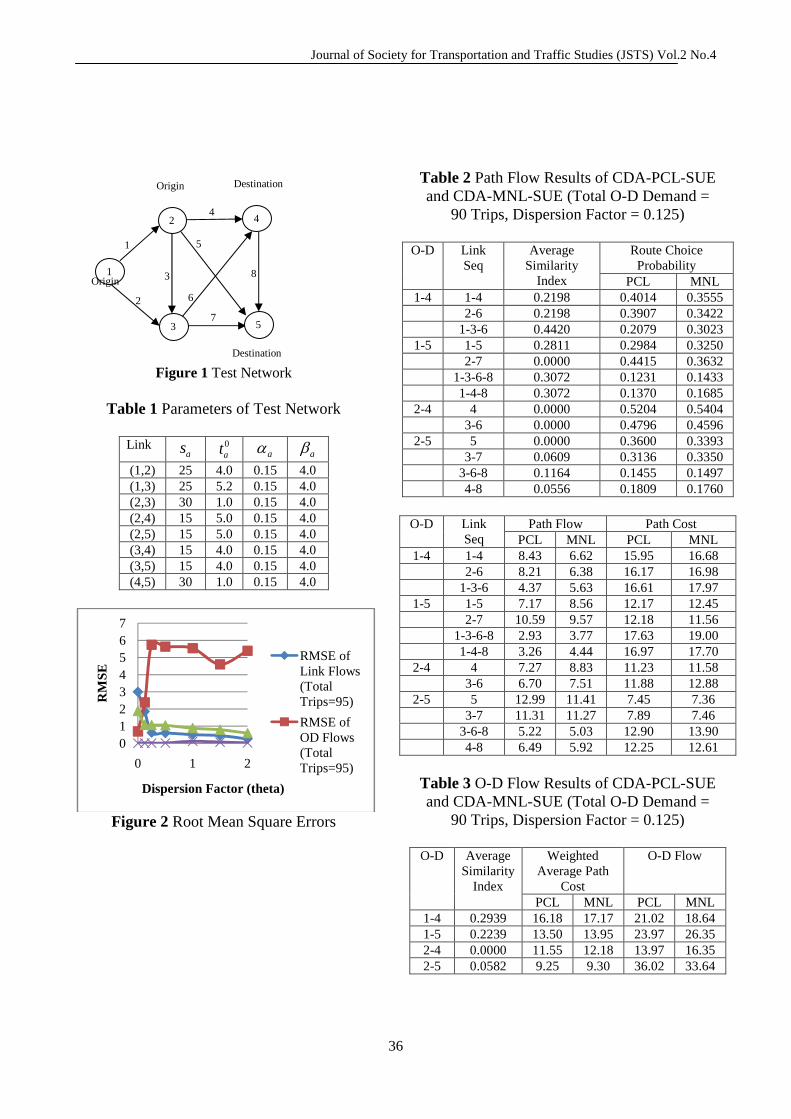
Journal of Society for Transportation and Traffic Studies (JSTS) Vol.2 No.4
36
Figure 1 Test Network
Table 1 Parameters of Test Network
Link as 0
at aα aβ
(1,2) 25 4.0 0.15 4.0 (1,3) 25 5.2 0.15 4.0 (2,3) 30 1.0 0.15 4.0 (2,4) 15 5.0 0.15 4.0 (2,5) 15 5.0 0.15 4.0 (3,4) 15 4.0 0.15 4.0 (3,5) 15 4.0 0.15 4.0 (4,5) 30 1.0 0.15 4.0
Figure 2 Root Mean Square Errors
Table 2 Path Flow Results of CDA-PCL-SUE and CDA-MNL-SUE (Total O-D Demand =
90 Trips, Dispersion Factor = 0.125)
O-D
Link Seq
Average Similarity
Index
Route Choice Probability
PCL MNL 1-4 1-4 0.2198 0.4014 0.3555
2-6 0.2198 0.3907 0.3422 1-3-6 0.4420 0.2079 0.3023
1-5 1-5 0.2811 0.2984 0.3250 2-7 0.0000 0.4415 0.3632 1-3-6-8 0.3072 0.1231 0.1433 1-4-8 0.3072 0.1370 0.1685
2-4 4 0.0000 0.5204 0.5404 3-6 0.0000 0.4796 0.4596
2-5 5 0.0000 0.3600 0.3393 3-7 0.0609 0.3136 0.3350 3-6-8 0.1164 0.1455 0.1497 4-8 0.0556 0.1809 0.1760
O-D
Link Seq
Path Flow Path Cost PCL MNL PCL MNL
1-4 1-4 8.43 6.62 15.95 16.68 2-6 8.21 6.38 16.17 16.98 1-3-6 4.37 5.63 16.61 17.97
1-5 1-5 7.17 8.56 12.17 12.45 2-7 10.59 9.57 12.18 11.56 1-3-6-8 2.93 3.77 17.63 19.00 1-4-8 3.26 4.44 16.97 17.70
2-4 4 7.27 8.83 11.23 11.58 3-6 6.70 7.51 11.88 12.88
2-5 5 12.99 11.41 7.45 7.36 3-7 11.31 11.27 7.89 7.46 3-6-8 5.22 5.03 12.90 13.90 4-8 6.49 5.92 12.25 12.61
Table 3 O-D Flow Results of CDA-PCL-SUE and CDA-MNL-SUE (Total O-D Demand =
90 Trips, Dispersion Factor = 0.125)
O-D Average Similarity
Index
Weighted Average Path
Cost
O-D Flow
PCL MNL PCL MNL 1-4 0.2939 16.18 17.17 21.02 18.64 1-5 0.2239 13.50 13.95 23.97 26.35 2-4 0.0000 11.55 12.18 13.97 16.35 2-5 0.0582 9.25 9.30 36.02 33.64
01234567
0 1 2
RM
SE
Dispersion Factor (theta)
RMSE of Link Flows (Total Trips=95)
RMSE of OD Flows (Total Trips=95)
1
1
2
3
4
5
2
3
4
5
6
7
8 Origin
Origin
Destination
Destination
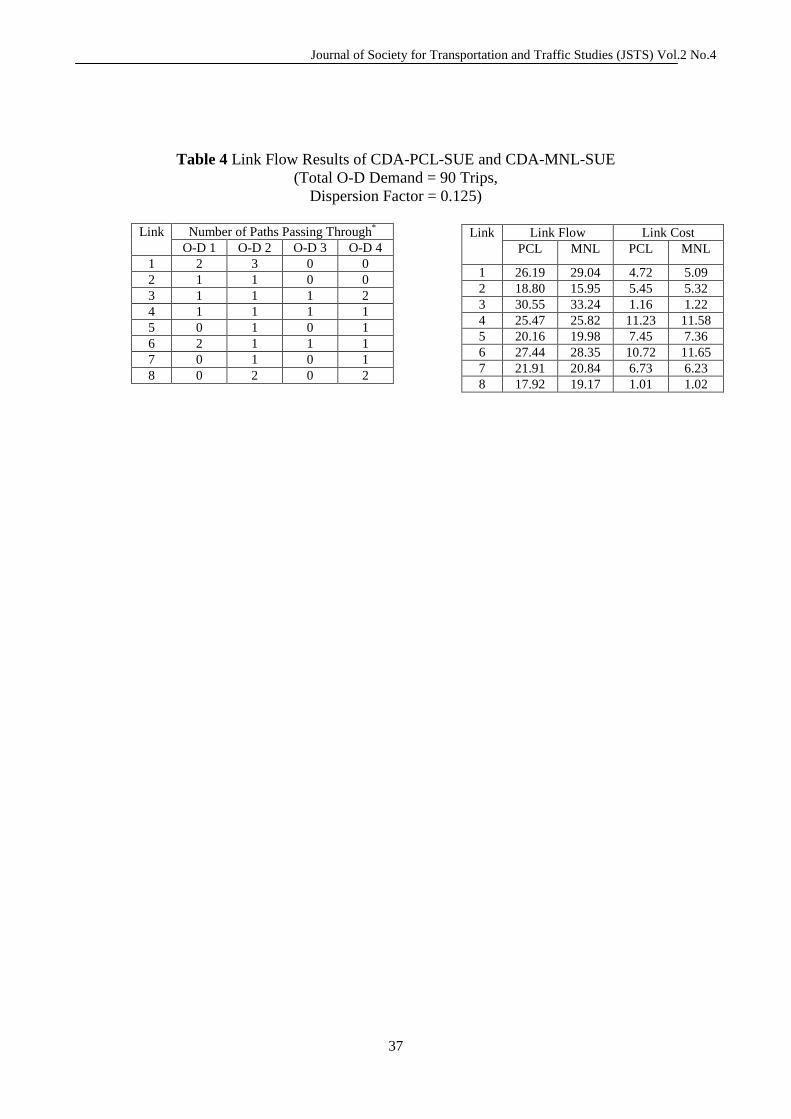
Journal of Society for Transportation and Traffic Studies (JSTS) Vol.2 No.4
37
Table 4 Link Flow Results of CDA-PCL-SUE and CDA-MNL-SUE (Total O-D Demand = 90 Trips,
Dispersion Factor = 0.125)
Link Number of Paths Passing Through* O-D 1 O-D 2 O-D 3 O-D 4
1 2 3 0 0 2 1 1 0 0 3 1 1 1 2 4 1 1 1 1 5 0 1 0 1 6 2 1 1 1 7 0 1 0 1 8 0 2 0 2
Link Link Flow Link Cost PCL MNL PCL MNL
1 26.19 29.04 4.72 5.09 2 18.80 15.95 5.45 5.32 3 30.55 33.24 1.16 1.22 4 25.47 25.82 11.23 11.58 5 20.16 19.98 7.45 7.36 6 27.44 28.35 10.72 11.65 7 21.91 20.84 6.73 6.23 8 17.92 19.17 1.01 1.02
Journal of Society for Transportation and Traffic Studies (JSTS)
38
REFERENCES
Bregman, L.M. (1967) The relaxation method of finding the common point of convex sets and its application to the solution of problems in convex programming, U.S.S.R. Computational Mathematics and Mathematical Physics, Vol.7, 200-217. Chen, A., P. Kasikitwiwat, and Z. Ji (2003) Solving the overlapping problem in route choice with paired combinatorial logit model, Transportation Research Record 1857, 65-73. Daganzo, C.F. and Y. Sheffi (1977) On Stochastic Models of Traffic Assignment, Transportation Science, Vol.11, 253-274. Damberg, O., J.T. Lundgren and M. Patriksson (1996) An algorithm for the stochastic user equilibrium problem, Transportation Research Part B, Vol.30, 115-131. Erlander, S. (1990) Efficient behavior and the simultaneous choices of origins, destinations and routes, Transportation Research Part B, Vol.24, 363-373. Evans, S.P. (1976) Derivation and analysis of some models for combining trip distribution and assignment, Transportation Research, Vol.10, 37-57. Lamond, B. and N.F. Stewart (1981) Bregman’s Balancing Method, Transportation Research Part B, Vol.15, No.4, 239-248. Larsson, T. and M. Patriksson (1992) Simplicial decomposition with disaggregated representation for the traffic assignment problem, Transportation Science, Vol.26, 4-17. Lundgren, J.T. and M. Patriksson (1998) The combined distribution and stochastic assignment problem, Annals of Operations Research, Vol.82, 309-329. Prashker, J.N. and S. Bekhor (2000) Congestion, Stochastic, and Similarity Effects in Stochastic User- Equilibrium Models, Transportation Research Record 1733, 80-87. Patriksson, M. (1993) Partial linearization methods in nonlinear programming, Journal of Optimization Theory and Applications, Vol.78, 227-246.
Journal of Society for Transportation and Traffic Studies (JSTS)
39
THAI GUIDELINE FOR THE DESIGN OF SIGNAL CONTROL AT INTERSECTIONS – INTRODUCTION
TO APPLIED PRELIMINARY CAPACITY ANALYSIS METHO D
ABSTRACT: The partner universities of the international scientific network «NICE on RoadS – EU-Asia Network in Competence Enhancement on Road Safety» developed a «Thai Guideline for the Design of Signal Control at Intersections». The guideline was prepared in the framework of the Thai-E.C. project «Improving Road Traffic Safety in Thailand – A Common Challenge for European and Thai Universities» based on international technology and knowledge transfer. This paper gives an introduction to the Preliminary Capacity Analysis Method (PCA-Method), which is introduced in the developed guideline. The theoretical background of the PCA-Method and the related analysis steps will be introduced in this paper. Furthermore the application of the PCA-Method will be explained by a practical example. KEY WORDS: signal control, road safety, preliminary capacity analysis 1. INTRODUCTION The partner universities of the international scientific network «NICE on RoadS» developed a «Thai Guideline for the Design of Signal Control at Intersections» based on international technology and knowledge transfer (Vesper et al., 2010b). The guideline was developed in the framework of the Thai-E.C. project «Improving Road Traffic Safety in Thailand – A Common Challenge for European and Thai Universities».
This paper gives an introduction to the Preliminary Capacity Analysis Method (PCA-Method), which is introduced in the developed guideline for preliminary capacity analysis of signal control at intersection. The introduced PCA-Method is based on the German «AKF-Method» (Mueller, 1969). It is a simple and very effective method to estimate whether available capacity is sufficient to serve traffic volumes at signalised intersections or not.
Andreas VESPER Senior Researcher Department of Transport Planning And Traffic Engineering Bauhaus-University Weimar Marienstrasse 13 C 99423 Weimar, Germany Fax: +49-3643-58-4475 E-mail: [email protected]
Pichai TANEERANANON Professor Centre for Road Safety Research Department of Civil Engineering Prince of Songkla University Hat Yai 90112 Thailand Fax: +66-74-446519 E-mail: [email protected]

Journal of Society for Transportation and Traffic Studies (JSTS)
40
2. DESIGN OF SIGNAL CONTROL 2.1 Control levels The following two control levels can be distinguished in traffic control at signalised intersections:
• Area Control Level (macroscopic level), • Local Control Level (microscopic level).
On the area control level, control strategies are defined which are effective for several signalised intersections located in an area, like e.g. in a road section, district or even in a whole city. Whereas the local control level comprises signal control at a local single intersection. Here local control decisions are only effective for road users crossing the respective signalised intersection. The prepared «Thai Guideline for the Design of Signal Control at Intersections» focuses mainly on the design of signal control on local control
level. This means the design of signal control at local intersection. 2.2 Work-flow for the design of signal control The design of signal control at local intersection can be subdivided in four design phases as introduced in the new «Thai Guideline for the Design of Signal Control at Intersections». Following this guideline the mentioned phases can be conducted successively in the design process of signal control as follows:
• Collection of Basic Design Data, • Preliminary Capacity Analysis of Signal
Control, • Capacity Analysis of Signal Control, • Final Check of Signal Control.
The work-flow for the design of signal control at local intersection (see Figure 1) gives an overview of the four design phases, the related sub-steps and the interrelation between them.
Figure 1 Work-flow for the Design of Signal Control at Local Intersection, (NICE on RoadS, 2011)
Layout plan1st phase
Collection of basic design data
Preliminary Capacity Analysis (PCA)
Fixeddesign
Draftdesign
Traffic volume
Signalcontrol
Geometricdesign
Control level
No areacontrol
Areacontrol
Co-ordination
No greenwave
Green wave
2nd phasePreliminary
capacity analysisof signal control
not successfulPreliminary Capacity Analysis (PCA) Modification of basic design data
like e.g. number of lanes etc.
successful
3rd phaseCapacity analysisof signal control
Determination of number of phases
Determination of signal groups
Calculation of intergreen-times
Determination of phase sequence
Calculation of GREEN-times
Determination of signal program
Calculation of cycle time
4th phaseFinal check
of signal control
Final check based on check list
Road safety audit
Determination of type of signal control
not successful
in case deficits arerelated to the capacity
analysis of signalcontrol
in case deficitsare related to
basic design data
Determination of AMBER-times
Check of RED-times
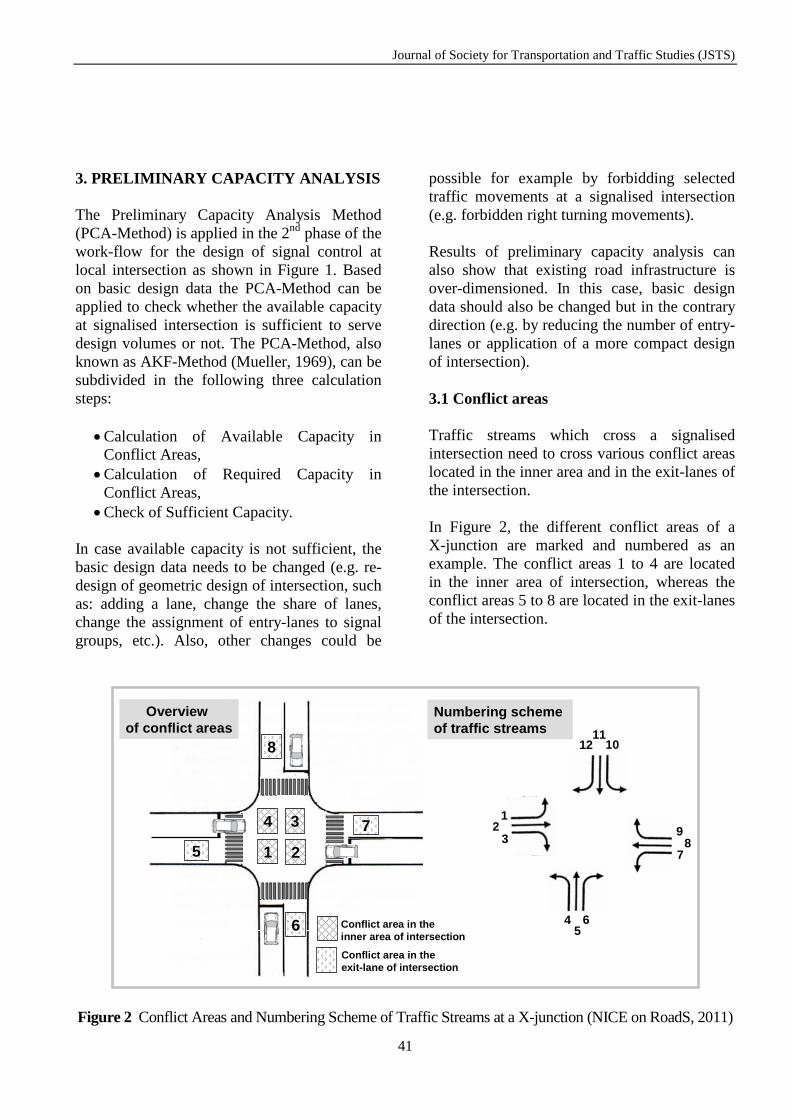
Journal of Society for Transportation and Traffic Studies (JSTS)
41
3. PRELIMINARY CAPACITY ANALYSIS The Preliminary Capacity Analysis Method (PCA-Method) is applied in the 2nd phase of the work-flow for the design of signal control at local intersection as shown in Figure 1. Based on basic design data the PCA-Method can be applied to check whether the available capacity at signalised intersection is sufficient to serve design volumes or not. The PCA-Method, also known as AKF-Method (Mueller, 1969), can be subdivided in the following three calculation steps:
• Calculation of Available Capacity in Conflict Areas,
• Calculation of Required Capacity in Conflict Areas,
• Check of Sufficient Capacity. In case available capacity is not sufficient, the basic design data needs to be changed (e.g. re-design of geometric design of intersection, such as: adding a lane, change the share of lanes, change the assignment of entry-lanes to signal groups, etc.). Also, other changes could be
possible for example by forbidding selected traffic movements at a signalised intersection (e.g. forbidden right turning movements). Results of preliminary capacity analysis can also show that existing road infrastructure is over-dimensioned. In this case, basic design data should also be changed but in the contrary direction (e.g. by reducing the number of entry-lanes or application of a more compact design of intersection). 3.1 Conflict areas Traffic streams which cross a signalised intersection need to cross various conflict areas located in the inner area and in the exit-lanes of the intersection. In Figure 2, the different conflict areas of a X-junction are marked and numbered as an example. The conflict areas 1 to 4 are located in the inner area of intersection, whereas the conflict areas 5 to 8 are located in the exit-lanes of the intersection.
Figure 2 Conflict Areas and Numbering Scheme of Traffic Streams at a X-junction (NICE on RoadS, 2011)
1
4 3
25
7
6
8
12
39
87
45
6
1211
10
Conflict area in the inner area of intersection
Conflict area in the exit-lane of intersection
Overviewof conflict areas
Numbering schemeof traffic streams

Journal of Society for Transportation and Traffic Studies (JSTS)
42
3.2 Available capacity in conflict areas The calculation of available capacity in conflict areas is the first calculation-step of PCA-Method. The available capacity in conflict areas is limited and can be calculated as shown in Formula 1:
h
estimatediC
PCA t
tt
Cavail∑−
=,*
36003600
.
(Eq.1) legend: avail. CPCA
: available capacity in conflict areas; [pcu/h]
tC : cycle time; [s/cycle] Σti, estimated : total estimated intergreen-time per
cycle; [s/cycle]
th : mean time headway; [s/pcu] For preliminary capacity analysis an estimated intergreen-time (ti, estimated) of 6 to 7 s per phase-transition can be applied. Here one should consider that estimated intergreen-times are only applicable for preliminary capacity analysis and not for capacity analysis of signal
control in the 3rd phase of the work-flow (see Figure 1). For preliminary capacity analysis a mean time headway of 1,8 to 2,2 s per pcu can be applied. The mean time headway can differ significantly depending on the location and the geometric design of intersection. For this reason this parameter needs to be determined based on an onsite data inspection. The choice of cycle time (tC) has a strong influence on the available capacity in conflict areas (avail. CPCA). The interrelation between the mentioned two parameters is shown in Figure 3 for different total intergreen-times per cycle. The diagram clarifies obviously that in case of low cycle times (up to ~70 seconds), the increase of cycle time has a great influence on available capacity in conflict areas at signalised intersections. In contrast, higher cycle times have an increasingly smaller influence on available capacity e.g. in a range over ~120 seconds. For this reason it is recommended to apply cycle times in a range between 30 and 90 s as a regular solution and only in exceptional cases in a range between 90 up to 120 s. Cycle times higher than 120 s should be avoided.
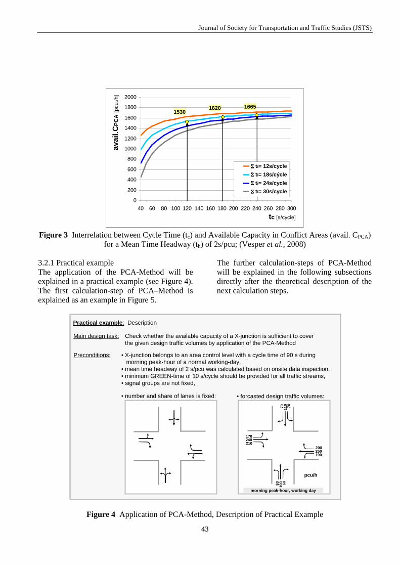
Journal of Society for Transportation and Traffic Studies (JSTS)
43
Figure 3 Interrelation between Cycle Time (tc) and Available Capacity in Conflict Areas (avail. CPCA)
for a Mean Time Headway (th) of 2s/pcu; (Vesper et al., 2008) 3.2.1 Practical example The application of the PCA-Method will be explained in a practical example (see Figure 4). The first calculation-step of PCA–Method is explained as an example in Figure 5.
The further calculation-steps of PCA-Method will be explained in the following subsections directly after the theoretical description of the next calculation steps.
Figure 4 Application of PCA-Method, Description of Practical Example
0
200
400
600
800
1000
1200
1400
1600
1800
2000
40 60 80 100 120 140 160 180 200 220 240 260 280 300
tz = 12stz = 18stz = 24stz = 30s
tc [s/cycle]
avai
l.CP
CA
[pcu
./h]
15301620 1665
Σ Σ Σ Σ t i= 12s/cycle
Σ Σ Σ Σ t i= 18s/cýcle
Σ Σ Σ Σ t i= 24s/cycle
Σ Σ Σ Σ t i= 30s/cycle
Practical example: Description
Main design task: Check whether the available capacity of a X-junction is sufficient to coverthe given design traffic volumes by application of the PCA-Method
Preconditions: • X-junction belongs to an area control level with a cycle time of 90 s duringmorning peak-hour of a normal working-day,
• mean time headway of 2 s/pcu was calculated based on onsite data inspection,• minimum GREEN-time of 10 s/cycle should be provided for all traffic streams,• signal groups are not fixed,
• number and share of lanes is fixed: • forcasted design traffic volumes:
200250190
170240210
6080 100
7070 110
pcu/h
morning peak-hour, working day
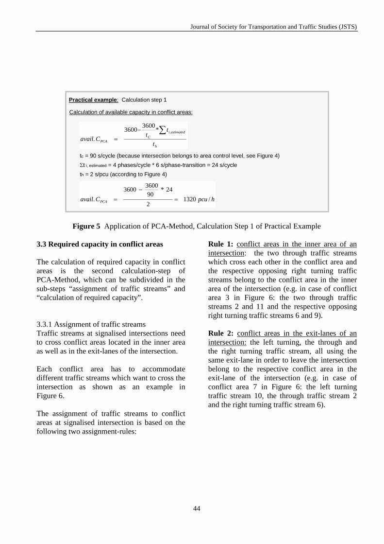
Journal of Society for Transportation and Traffic Studies (JSTS)
44
Figure 5 Application of PCA-Method, Calculation Step 1 of Practical Example 3.3 Required capacity in conflict areas The calculation of required capacity in conflict areas is the second calculation-step of PCA-Method, which can be subdivided in the sub-steps “assignment of traffic streams” and “calculation of required capacity”. 3.3.1 Assignment of traffic streams Traffic streams at signalised intersections need to cross conflict areas located in the inner area as well as in the exit-lanes of the intersection. Each conflict area has to accommodate different traffic streams which want to cross the intersection as shown as an example in Figure 6. The assignment of traffic streams to conflict areas at signalised intersection is based on the following two assignment-rules:
Rule 1: conflict areas in the inner area of an intersection: the two through traffic streams which cross each other in the conflict area and the respective opposing right turning traffic streams belong to the conflict area in the inner area of the intersection (e.g. in case of conflict area 3 in Figure 6: the two through traffic streams 2 and 11 and the respective opposing right turning traffic streams 6 and 9). Rule 2: conflict areas in the exit-lanes of an intersection: the left turning, the through and the right turning traffic stream, all using the same exit-lane in order to leave the intersection belong to the respective conflict area in the exit-lane of the intersection (e.g. in case of conflict area 7 in Figure 6: the left turning traffic stream 10, the through traffic stream 2 and the right turning traffic stream 6).
Practical example: Calculation step 1
Calculation of available capacity in conflict areas:
h
estimatediC
PCA t
tt
Cavail∑−
=,*
36003600
.
tc = 90 s/cycle (because intersection belongs to area control level, see Figure 4)
Σt i, estimated = 4 phases/cycle * 6 s/phase-transition = 24 s/cycle
th = 2 s/pcu (according to Figure 4)
hpcuCavail PCA /13202
24*90
36003600
. =
−
=
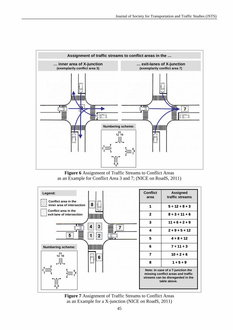
Journal of Society for Transportation and Traffic Studies (JSTS)
45
Figure 6 Assignment of Traffic Streams to Conflict Areas
as an Example for Conflict Area 3 and 7; (NICE on RoadS, 2011)
Figure 7 Assignment of Traffic Streams to Conflict Areas as an Example for a X-junction (NICE on RoadS, 2011)
3
Assignment of traffic streams to conflict areas in the …
7
… inner area of X-junction(exemplarily conflict area 3)
… exit-lanes of X-junction(exemplarily conflict area 7)
Numbering scheme:
Conflict area in the inner area of intersection
Conflict area in the exit-lane of intersection
1 + 5 + 98
Note: In case of a T-junction themissing conflict areas and traffic
streams can be disregarded in the table above.
10 + 2 + 67
7 + 11 + 36
4 + 8 + 125
2 + 9 + 5 + 124
11 + 6 + 2 + 93
8 + 3 + 11 + 62
5 + 12 + 8 + 31
Assignedtraffic streams
Conflictarea
1 + 5 + 98
Note: In case of a T-junction themissing conflict areas and traffic
streams can be disregarded in the table above.
10 + 2 + 67
7 + 11 + 36
4 + 8 + 125
2 + 9 + 5 + 124
11 + 6 + 2 + 93
8 + 3 + 11 + 62
5 + 12 + 8 + 31
Assignedtraffic streams
Conflictarea
Numbering scheme:
Legend:

Journal of Society for Transportation and Traffic Studies (JSTS)
46
In Figure 7 the different conflict areas and the assigned traffic streams are shown as an example for a X-junction. This table is also applicable for T-junctions. In case of a T-junction, the missing conflict areas and traffic streams need to be disregarded. 3.3.2 Calculation of required capacity The required capacity in conflict areas depends:
• on the assigned traffic streams of conflict areas as shown in Figure 7
• and on the relevant design volume of traffic streams.
The relevant design volume of traffic streams (rel. Vi) can be determined based on basic design data and further requirements of signal control such as:
• design volume of traffic streams (Vi), • share of lanes in the entries of intersection
(exclusive or shared lanes; one or more lanes per direction)
• and the assignment of entry-lanes and related traffic streams to signal groups (here one should consider that one signal group can cover one or more entry-lanes, which can cover one or more traffic streams).
• The determination of relevant design volume of traffic streams is explained in Figure 8.
The required capacity in conflict areas can be calculated based on Formula 2 according to Figure 8.
∑= kikCA VrelCreq ,.. (Eq.2)
legend: req. CCA
k
: required capacity in conflict area k; [pcu/(h*conflict area)]
k : number of conflict area as shown in Figure 7; [-]
rel. Vi : relevant design volume of traffic stream i as introduced in Figure 8; [pcu/(h*entry-lane)]
Σrel. Vi, k : total amount of relevant design volumes of the traffic streams which are assigned to conflict area k as shown in Figure 7; [pcu/(h*conflict area)]
i : number of traffic stream according to numbering scheme as shown in Figure 7; [-]

Journal of Society for Transportation and Traffic Studies (JSTS)
47
Figure 8 Determination of Relevant Design Volume of Traffic Streams (rel Vi) – overview (NICE on RoadS, 2011)
The main parameter in the calculation of the required capacity in conflict areas (req. CCA k) is the relevant design volume of traffic streams (rel. Vi) at the considered intersection. The share of lanes and the assignment of traffic streams to signal groups need to be considered in the calculation of relevant design volume of traffic streams (rel. Vi) as introduced in Figure 8 and Formula 3. (Eq.3) legend: rel. Vi : relevant design volume of traffic
stream i as introduced in Figure 8; [pcu/(h*entry-lane)]
V i : design volume of traffic stream i;
[pcu/(h*traffic stream)] i : number of traffic stream according to
numbering scheme as shown in Figure 7; [-]
RVj : relevant design volume of entry-lane which covers traffic stream j; [pcu/(h*entry-lane)]
j : number of traffic stream according to numbering scheme as shown in Figure 7; [-]
RVm, s : relevant design volume of signal groups which covers traffic stream m; [pcu/(h*entry-lane)]
s : signal group which covers traffic stream m; [-]
m : number of traffic stream according to numbering scheme as shown in Figure 7; [-]
Furthermore, it should be ensured that minimum GREEN-times (min tgr) will be considered in the preliminary capacity analysis
Share of lanes
Signal groups
Vi
TVj=ΣVi TVj=ΣVi
rel. Vi = Vi
TVk,s = max(TVj)
rel. Vi = TVj(for i=j)
rel. Vi = TVk,s(for i=k)
not fixed
not fixed
not fixed
fixed fixed
fixed
Basic data design traffic volume of traffic streams
ViVi
relevant design traffic volume of traffic streams
Relevant datafor PCA
rel. Vi = RVm,s(for i=m)
RVm,s = max(RVj)
Share of entry-lanes RVj = ΣViRVj = ΣVi
rel. Vi = RVj(for i=j)
Relevant design volume of traffic streams
Design volume of traffic streams
=
==
)(
)(.
, miRV
jiRV
V
Vrel
sm
j
i
i
standard
for i=j in case the share of entry-lanes is fixedfor i=m in case the share ofentry-lanes and thesignal groups are fixed

Journal of Society for Transportation and Traffic Studies (JSTS)
48
of signal control by the check that relevant design volume of traffic streams is higher than minimum relevant design volume of traffic streams (min rel. Vi) according to Formula 4:
h
gr
cii t
t
tVrelVrel
min*
3600.min. =≥ (Eq.4)
legend: rel. Vi : relevant design volume of traffic
stream i as introduced in Figure 8; [pcu/(h*entry-lane)]
min rel. Vi
: minimum relevant design volume of traffic stream i, considering minimum GREEN-time per cycle (min tgr);[pcu/(h*entry-lane)]
i : number of traffic stream according to numbering scheme as shown in Figure 7;[-]
tc : cycle time; [s/cycle] min tgr : minimum GREEN-time which
should be applied in signal program design; [s]
th : mean time headway; [s/pcu] In case where the share of entry-lanes is pre-defined, and thereby fixed, the relevant design volume of entry-lane which covers the traffic streams (RVj) needs to be considered in
preliminary capacity analysis, as introduced in Figure 8 and Formula 3. The relevant design volume of entry-lane which covers the traffic stream j (RVj) can be calculated according to Formula 5.
(Eq.5) legend: RVj : relevant design volume of entry-lane
which covers traffic stream j; [pcu/(h*entry-lane)]
j : number of traffic stream according to numbering scheme as shown in
Figure 7; [-] V i : design volume of traffic stream i;
[pcu/(h*traffic stream)] i : number of traffic stream according to
numbering scheme as shown in Figure 7; [-]
The calculation of the relevant design volume of entry-lanes (RVj) is explained as an example in Figure 9.
∑= ij VRVfor traffic streams i whichbelong to the entry-lanewhich covers traffic stream j

Journal of Society for Transportation and Traffic Studies (JSTS)
49
Figure 9 Relevant Design Volume of Entry-lanes (RVj) and the Design Volume of Related Traffic Streams (Vi); (NICE on RoadS, 2011)
In case of high pedestrian traffic volumes, it should be proved whether design volumes Vi of turning traffic streams need to be increased because turning vehicles should give the priority to crossing pedestrians in the exit-lanes of intersection. In case of two or more entry-lanes for one traffic stream, the split of traffic volumes between the two or more parallel lanes is relevant for calculation of the relevant design volume (RVj) of each lane. For a first preliminary calculation, a proportional split is applicable in most cases. In case where signal groups at signalised intersections are already fixed and cannot be changed, the relevant design volume of signal group s which covers traffic stream m (RVm,s) needs to be considered in preliminary capacity
analysis, as introduced in Figure 8 and Formula 3. Here, the relevant design volume of signal group s which can cover several traffic streams is equal to the maximum value of relevant design volumes of the covered entry-lanes (shared or exclusive lanes), as defined in Formula 6.
(Eq.6) legend: RVm ,s : relevant design volume of signal
group s which covers traffic stream m; [pcu/(h*entry-lane)];
s : number of signal group (e.g. V1, V2, …); [-]
Numbering scheme:
RV4 = V4RV5 = V5RV6 = V6
RV4 = V4RV5 = V5 + V6RV6 = V5 + V6
RV4 = V4 + V5RV5 = V4 + V5
RV6 = V6
RV4 = V4 + V5 + V6RV5 = V4 + V5 + V6RV6 = V4 + V5 + V6
RV1 = V1RV2 = V2RV3 = V3
RV1 = V1RV2 = V2 + V3RV3 = V2 + V3
RV1 = V1 + V2
RV2 = V1 + V2RV3 = V3
RV1 = V1 + V2 + V3RV2 = V1 + V2 + V3RV3 = V1 + V2 + V3
Relevant design volumeof entry-lane (RV j)
covering traffic stream j
Share of entry-lanes
RV10 = V10RV11 = V11RV12 = V12
RV10 = V10RV11 = V11 + V12RV12 = V11 + V12
RV10 = V10 + V11RV11 = V10 + V11
RV12 = V12
RV10 = V10 + V11 + V12RV11 = V10 + V11 + V12RV12 = V10 + V11 + V12
RV7 = V7RV8 = V8RV9 = V9
RV7 = V7RV8 = V8 + V9RV9 = V8 + V9
RV7 = V7 + V8RV8 = V7 + V8
RV9 = V9
RV7 = V7 + V8 + V9RV8 = V7 + V8 + V9RV9 = V7 + V8 + V9
Relevant design volumeof entry-lane (RV j)
covering traffic stream j
Share of entry-lanes
Explanatoryexample:
RV1=RV2RV3
V3
V2
V1
2 Lanes in the entry:-1 Shared left turning/
through lane with a relevant design volumeof RV1=RV2 =V1+V2
-1 Exclusive right turning lane with a relevant designvolume of RV 3 = V3
RVj [pcu/(h*entry-lane]
Vi [pcu/(h*traffic stream]
( )jsm RVRV max, =for traffic streams jwhich belong tosignal group s
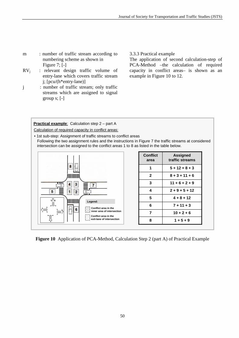
Journal of Society for Transportation and Traffic Studies (JSTS)
50
m : number of traffic stream according to numbering scheme as shown in
Figure 7; [-] RVj : relevant design traffic volume of
entry-lane which covers traffic stream j; [pcu/(h*entry-lane)]
j : number of traffic stream; only traffic streams which are assigned to signal group s; [-]
3.3.3 Practical example The application of second calculation-step of PCA-Method –the calculation of required capacity in conflict areas– is shown as an example in Figure 10 to 12.
Figure 10 Application of PCA-Method, Calculation Step 2 (part A) of Practical Example
Practical example: Calculation step 2 – part A
Calculation of required capacity in conflict areas:
• 1st sub-step: Assignment of traffic streams to conflict areasFollowing the two assignment rules and the instructions in Figure 7 the traffic streams at consideredintersection can be assigned to the conflict areas 1 to 8 as listed in the table below.
1 + 5 + 98
10 + 2 + 67
7 + 11 + 36
4 + 8 + 125
2 + 9 + 5 + 124
11 + 6 + 2 + 93
8 + 3 + 11 + 62
5 + 12 + 8 + 31
Assignedtraffic streams
Conflictarea
1 + 5 + 98
10 + 2 + 67
7 + 11 + 36
4 + 8 + 125
2 + 9 + 5 + 124
11 + 6 + 2 + 93
8 + 3 + 11 + 62
5 + 12 + 8 + 31
Assignedtraffic streams
Conflictarea
Conflict area in the inner area of intersection
Conflict area in the exit-lane of intersection
Legend:
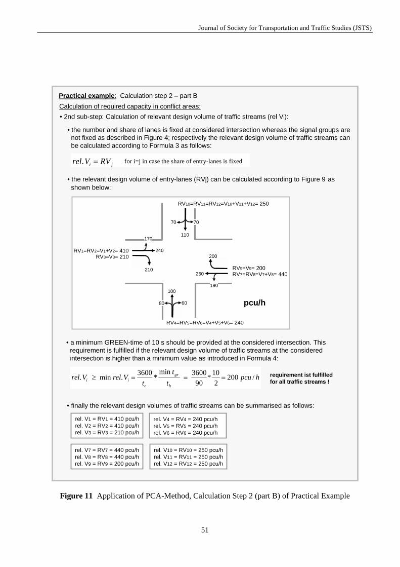
Journal of Society for Transportation and Traffic Studies (JSTS)
51
Figure 11 Application of PCA-Method, Calculation Step 2 (part B) of Practical Example
Practical example: Calculation step 2 – part B
Calculation of required capacity in conflict areas:
• 2nd sub-step: Calculation of relevant design volume of traffic streams (rel Vi):
• the number and share of lanes is fixed at considered intersection whereas the signal groups arenot fixed as described in Figure 4; respectively the relevant design volume of traffic streams canbe calculated according to Formula 3 as follows:
• the relevant design volume of entry-lanes (RVj) can be calculated according to Figure 9 as shown below:
RV1=RV2=V1+V2= 410RV3=V3= 210
RV7=RV8=V7+V8= 440RV9=V9= 200
RV10=RV11=RV12=V10+V11+V12= 250
RV4=RV5=RV6=V4+V5+V6= 240
pcu/h
100
6080
250
190
200
7070
110170
210
240
• a minimum GREEN-time of 10 s should be provided at the considered intersection. Thisrequirement is fulfilled if the relevant design volume of traffic streams at the consideredintersection is higher than a minimum value as introduced in Formula 4:
hpcut
t
tVrelVrel
h
gr
cii /200
2
10*
90
3600min*
3600.min. ===≥ requirement ist fulfilled
for all traffic streams !
• finally the relevant design volumes of traffic streams can be summarised as follows:
rel. V1 = RV1 = 410 pcu/hrel. V2 = RV2 = 410 pcu/hrel. V3 = RV3 = 210 pcu/h
rel. V4 = RV4 = 240 pcu/hrel. V5 = RV5 = 240 pcu/hrel. V6 = RV6 = 240 pcu/h
rel. V7 = RV7 = 440 pcu/hrel. V8 = RV8 = 440 pcu/hrel. V9 = RV9 = 200 pcu/h
rel. V10 = RV10 = 250 pcu/hrel. V11 = RV11 = 250 pcu/hrel. V12 = RV12 = 250 pcu/h
ji RVVrel =. for i=j in case the share of entry-lanes is fixed

Journal of Society for Transportation and Traffic Studies (JSTS)
52
Figure 12 Application of PCA-Method, Calculation Step 2 (part C) of Practical Example 3.4 Check of sufficient capacity The check of sufficient available capacity can be conducted based on the calculated available capacity in conflict areas and the required capacity in conflict areas. The check of sufficient capacity can be subdivided into the following two work-steps:
• Calculation of Available Degree of Saturation, • Capacity Check.
3.4.1 Available degree of saturation The available degree of saturation (ADS) is a value which describes which part of available capacity will be used by road users. The available degree of saturation (ADS) can be calculated by using Formula 7:
PCA
kCAk
Cavail
CreqADS
.
.= (Eq.7)
Practical example: Calculation step 2 – part C
Calculation of required capacity in conflict areas:
• 3rd sub-step: Calculation of required capacity in conflict areas (req. CCAk):
• the required capacity in conflict areas (req. CCAk) can be calculated based on Formula 2 as follows:
∑= kikCA VrelCreq ,..
• the required capacity in conflict areas (req. CCAk) can be calculated based on assigned trafficstreams to conflict areas (see Figure 10) and related relevant design volume of traffic streams(rel Vi; see Figure 11) as shown below:
� the maximum required capacity in conflict areas is required in conflict areas 1 and 2 as marked in the figure above.
rel.V1= rel.V2= 410rel.V3= 210
rel.V7= rel.V8= 440rel.V9= 200
rel.V10= rel.V11= rel.V12= 250
rel.V4= rel.V5= rel.V6= 240pcu/h
5
6
8
7
1 2
4 3
req.CCA5= 240+440+250= 930
req.CCA1= 240+250+440+210= 1140
req.CCA6= 440+250+210= 900
req.CCA2= 440+210+250+240= 1140
req.CCA7= 250+410+240= 900
req.CCA3= 250+240+410+200= 1100
req.CCA8= 410+240+200= 850
req.CCA4= 410+200+240+250= 1100

Journal of Society for Transportation and Traffic Studies (JSTS)
53
legend: ADSk : available degree of saturation in
conflict area k; [-] req. CCA k
: required capacity in conflict area k; [pcu/(h*conflict area)]
avail. CPCA
: available capacity in conflict areas; [pcu/(h*conflict area)]
k : number of conflict area as shown in Figure 7; [-]
3.4.2 Capacity check Because of randomness of arriving vehicles in the entries of signalised intersections, the target degree of saturation (TDS) in the design of signal control should be at maximum:
(Eq.8) legend: TDS : target degree of saturation [-] Following this requirement, a signalised intersection is said to provide sufficient capacity if the requirement in Formula 9 is fulfilled:
(Eq.9) legend: ADSk : available degree of saturation in
conflict area k; [k] k : number of conflict area as shown
in Figure 7; [-] TDS : target degree of saturation [-] The limiting TDS (see Formula 8) ensures that approaching road users will be served at signalised intersection within cycle time. Furthermore the limiting TDS for co-ordinated intersections ensures that progression speed can be maintained for co-ordinated traffic streams. In case where the main parameters of the preliminary capacity analysis will also be applied in the design of signal program, it can be expected that the detailed signal program calculation will be successful too. The main parameters of the preliminary capacity analysis are amongst others:
• Design of Intersection (number and share of entry-lanes (shared/exclusive)),
• Assignment of Entry-lanes to Signal Groups, • Cycle Time (tc), • Target Degree of Saturation (TDS).
If the available capacity is not sufficient, the basic design data needs to be modified or changed (see work-flow in Figure 1). Based on changed basic design data, the preliminary capacity analysis can be conducted again in order to prove that the available capacity is sufficient under the changed condition. 3.4.3 Practical example The application of third calculation step of PCA-Method –the check of sufficient capacity– is shown as an example in Figure 13.
≤
≤=
0.85to0.80
0.90to0.85TDS
in case of notco-ordinated intersections
in case of co-ordinated intersections
TDSADSk ≤

Journal of Society for Transportation and Traffic Studies (JSTS)
54
Figure 13 Application of PCA-Method, Calculation Step 3 of Practical Example
4. CONCLUSION The theoretical background of the Preliminary Capacity Analysis Method (PCA-Method) is introduced in this paper in detail. Furthermore the different calculation steps of the PCA-Method are explained for a signalised X-junction as a practical example. Beside the introduced PCA-Method the new developed «Thai Guideline for the Design of Signal Control at Intersections» comprises further main parts, which should be applied in the design of signal control. These are the “Collection of Basic Design Data”, the “Capacity Analysis of Signal Control” and the “Final Check of Signal Control” as introduced in the work-flow in Figure 1. Altogether the new developed «Thai Guideline for the Design of Signal Control at Intersections» provides a set of design instructions and recommendations which will help Thai engineers and practitioners to improve signal control at signalised intersections in the future.
It is expected that improved signal control will contribute to safer and more efficient use of signal control at intersections and thereby to contribute to improve road traffic safety as well as quality flow in the road network. 5. FORECAST The partner universities of the international network «NICE on RoadS» prepared the «Thai Guideline for the Design of Signal Control at Intersections» in the framework of of the Thai-E.C. project «Improving Road Traffic Safety in Thailand – A Common Challenge for European and Thai Universities». The guidelines will be published as an English version very soon and will be ready for application in practice afterwards. Furthermore the Thai partner universities will develop a Thai version of the guideline by the end of 2011. In this way the guideline will also be available in Thai language.
Practical example: Calculation step 3
Check of sufficient capacity:
• the maximum required capacity in conflict areas is required in conflict area 1 and 2 as shownin Figure 12. If the capacity check is successful for these two conflict areas, the check will be also successful for the other conflict areas.
86,01320
1140
.
. 11 ===
PCA
CA
Cavail
CreqADS
• the available degree of saturation can be calculated for conflict area 1 and 2 based on Formula 7:
• the capacity check is successful in case the requirement of Formula 9 is fulfilled:
90,085,086,0 −≤
� the capacity check is successful for conflict area 1 and 2� the capacity check is also successful for other conflict areas, because their ADSk is lower
than in the conflict areas 1 and 2.
�
86,012 == ADSADS
ordinatedconotTDSADSADS −≤= 21 not co-ordinated intersection

Journal of Society for Transportation and Traffic Studies (JSTS)
55
In May 2011 the partner universities of «NICE on RoadS» established the “EU-Asia Road Safety Centre of Excellence – RoSCoE”, which is located on the Hat Yai campus of the Prince of Songkla University in the south of Thailand. Here 6 PhD scholars are conducting their PhD-study, dealing with several road safety related aspects of road design. It is planned that they summarise results of their studies in design guidelines. In this way further design guidelines will be available for Thai engineers and practitioners for application in the future.
ACKNOWLEDGEMENTS The authors express their gratitude to the European Commission for the generous financial support to carry out this important research work in the framework of the Thai-E.C. project «Improving Road Traffic Safety in Thailand – A Common Challenge for European and Thai Universities».

Journal of Society for Transportation and Traffic Studies (JSTS)
56
REFERENCES Kolks, W., Fiedler, J. (2003) Verkehrswesen in der kommunalen Praxis, Vol. 1, 2nd edition, Erich
Schmidt Verlag, Berlin, Germany Mueller, P. (1969) Bemessung von Knotenpunkten mit Lichtsignalanlage mit Hilfe von
Konfliktbelastungen. Straßenverkehrstechnik 13/1969, Kirschbaum Verlag, Bonn, Germany NICE on RoadS (2011) Thai Guideline for the Design of Signal Control at Intersection, edited by
the international scientific network «NICE on RoadS – EU-Asia Network in Competence Enhancement on Road Safety», English version, final draft version, unpublished
Schnabel, W., Lohse, D. (2011) Grundlagen der Straßenverkehrstechnik und der Verkehrsplanung, 3rd edition, edited by DIN Deutsches Institut für Normung e.V., Beuth Verlag, Berlin in cooperation with Kirschbaum Verlag, Bonn, Germany
Vesper, A., Taneerananon, P., Kanitpong, K., Iamtrakul, P., Brannolte, U., Koren, C. (2010a) Traffic Control at Signalised Intersections – Preparation of a Design Guideline for Thailand, Journal of Society for Transportation and Traffic Studies (JSTS), Vol.1 No.4, page 1-19, ISSN 1906- 8360, Thai Society for Transportation and Traffic Studies (TSTS), Thailand
Vesper, A., Taneerananon, P., Kanitpong, K., Iamtrakul, P., Brannolte, U., Koren, C. (2010b) Approach of a Methodology for Road Design Guideline Implementation in Thailand - Based on International Technology and Knowledge Transfer, Journal of Society for Transportation and Traffic Studies (JSTS), Vol. 1 No. 3, page 54-67, ISSN 1906-8360, Thai Society for Transportation and Traffic Studies (TSTS), Thailand
Vesper, A., Taneerananon, P., Brannolte, U., Moerner, J. v. (2009) Analysis of Traffic Flow in Coordinated Sections of Urban Road Networks by Application of up-to-date Low-Cost- Methods, Journal of Eastern Asia Society for Transportation Studies, Vol. 8, page 1780- 1795, ISSN 1881- 1124, Eastern Asia Society for Transportation Studies (EASTS), Asia Vesper, A., Brannolte U., Taneerananon, P., Chen, Y. (2008) Traffic control at signalised intersections
in Germany, China and Thailand – Some hints to improve road traffic safety, Proceedings of 13th International Conference of Hong Kong Society for Transportation Studies (HKSTS), Hong Kong, China