Journal of Nonlinear Mathematical Physics Volume 11, Number 4 (2004), 435–460 Wave Motion

Steady Water Waves

M D GROVES

Department of Mathematical Sciences, Loughborough University, Loughborough,LE11 3TU, UKE-mail: M. D. Groves@lboro.ac.uk

This article is part of the Proceedings of the meeting at the Mathematical Research Institute atOberwolfach (Germany) titled “Wave Motion”, which took place during January 25-31, 2004

1 Introduction

The classical water wave problem concerns the irrotational flow of a perfect fluid of unitdensity subject to the forces of gravity and surface tension. The fluid motion is describedby the Euler equations in a domain bounded below by a rigid horizontal bottom {y = −h}and above by a free surface which is described as a graph {y = η(x, z, t)}, where thefunction η depends upon the two horizontal spatial directions x, z and time t. In termsof an Eulerian velocity potential φ(x, y, z, t) the mathematical problem is to solve theequations

φxx + φyy + φzz = 0 − h < y < η, (1.1)

φy = 0 on y = −h, (1.2)

φy = ηt + ηxφx + ηzφz on y = η (1.3)

and

φt +1

2(φ2

x + φ2y + φ2

z) + gη

− T

[

ηx√

1 + η2x + η2

z

]

x

− T

[

ηz√

1 + η2x + η2

z

]

z

= B on y = η, (1.4)

where g and T are respectively the acceleration due to gravity and the coefficient of surfacetension and B is a constant called the Bernoulli constant. The above formulation describesthree-dimensional gravity-capillary waves on water of finite depth, but several variationsupon this theme are possible. Solutions which do not depend upon the spatial coordinatez are called two-dimensional water waves, solutions with T = 0 are called gravity wavesand the limiting case h → ∞ is the infinite-depth problem. There are also versions of thehydrodynamic problem which involve multiple layers of fluids with different densities, orindeed a single fluid with a continuous density stratification. Steady waves are water wavesof the special form η(x, z, t) = η(x− c1t, z− c2t), φ(x, y, t) = φ(x− c1t, y, z− c2t); in otherwords they are uniformly translating in the horizontal direction with velocity c = (c1, c2).In this paper we survey some recent mathematical results concerning steady water waves,and in keeping with convention we continue to write x and z as abbreviations for x− c1t,z − c2t.

Copyright c© 2004 by M D Groves

436 M D Groves

The steady water-wave problem is one of the classical problems in applied mathematics,and there is a huge and growing literature in this area. However the majority of publishedresults concentrate on numerical studies or approximations by simper model equations, andthere has been far less rigorous mathematical study of the complete hydrodynamic problemformulated above. A small number of explicit solutions are available, namely the spatiallyperiodic solutions for pure capillary waves (g = 0) found by Crapper [23] and Kinnersley[24] for respectively the infinite- and finite-depth problems, and Gerstner’s trochoidalwaves for the slightly different infinite-depth problem in which vorticity effects are included(see Constantin [15] for a discussion). Functional-analytic techniques for partial differentialequations are required to make further progress with the exact equations, and in thispaper we survey the currently available mathematical results. Numerical, modelling andstability issues are therefore beyond its scope. Within this narrower field we focus uponthree topics in which substantial progress has recently been made and which are likelyto witness further rapid growth. The topics are Stokes waves (two-dimensional periodicgravity waves on water of infinite depth), the application of spatial dynamics to two-dimensional gravity-capillary waves on water of finite depth, and three-dimensional steadywater waves.

2 Stokes waves

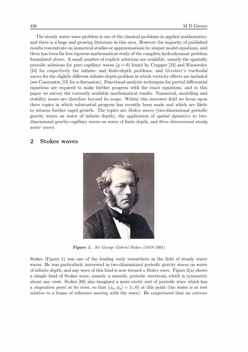
Figure 1. Sir George Gabriel Stokes (1819-1903)

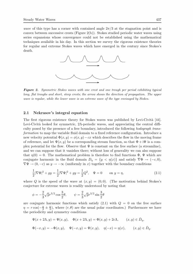
Stokes (Figure 1) was one of the leading early researchers in the field of steady waterwaves. He was particularly interested in two-dimensional periodic gravity waves on waterof infinite depth, and any wave of this kind is now termed a Stokes wave. Figure 2(a) showsa simple kind of Stokes wave, namely a smooth, periodic wavetrain which is symmetricabout any crest. Stokes [60] also imagined a more exotic sort of periodic wave which hasa stagnation point at its crest, so that (φx, φy) = (c, 0) at this point (the water is at restrelative to a frame of reference moving with the wave). He conjectured that an extreme

Steady Water Waves 437

wave of this type has a corner with contained angle 2π/3 at the stagnation point and isconvex between successive crests (Figure 2(b)). Stokes studied periodic water waves usingseries expansions whose convergence could not be established using the mathematicaltechniques available in his day. In this section we survey the rigorous existence theoriesfor regular and extreme Stokes waves which have emerged in the century since Stokes’sdeath.

Figure 2. Symmetric Stokes waves with one crest and one trough per period exhibiting typical

long, flat troughs and short, steep crests; the arrow shows the direction of propagation. The upper

wave is regular, while the lower wave is an extreme wave of the type envisaged by Stokes.

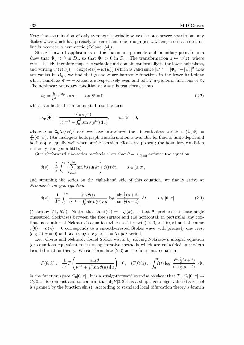
2.1 Nekrasov’s integral equation

The first rigorous existence theory for Stokes waves was published by Levi-Civita [44].Levi-Civita looked for symmetric, 2Λ-periodic waves, and appreciating the central diffi-culty posed by the presence of a free boundary, introduced the following hodograph trans-formation to map the variable fluid domain to a fixed reference configuration. Introduce anew velocity potential Φ(x, y) = φ(x, y)− cx which describes the flow in the moving frameof reference, and let Ψ(x, y) be a corresponding stream function, so that Φ + iΨ is a com-plex potential for the flow. Observe that Ψ is constant on the free surface (a streamline),and we can suppose that it vanishes there; without loss of generality we can also supposethat η(0) = 0. The mathematical problem is therefore to find functions Φ, Ψ which areconjugate harmonic in the fluid domain Dη = {y < η(x)} and satisfy ∇Φ → (−c, 0),∇Ψ → (0,−c) as y → −∞ (uniformly in x) together with the boundary conditions

1

2|∇Φ|2 + gy =

1

2|∇Ψ|2 + gy =

1

2Q2, Ψ = 0 on y = η, (2.1)

where Q is the speed of the wave at (x, y) = (0, 0). (The motivation behind Stokes’sconjecture for extreme waves is readily understood by noting that

φ = −2

3

√gr3/2 cos

3

2θ, ψ =

2

3

√gr3/2 sin

3

2θ

are conjugate harmonic functions which satisfy (2.1) with Q = 0 on the free surfaceη = r cos(−π

2 ± π3 ), where (r, θ) are the usual polar coordinates.) Furthermore we have

the periodicity and symmetry conditions

Ψ(x+ 2Λ, y) = Ψ(x, y), Φ(x+ 2Λ, y) = Φ(x, y) + 2cΛ, (x, y) ∈ Dη,

Φ(−x, y) = −Φ(x, y), Ψ(−x, y) = Ψ(x, y), η(−x) = η(x), (x, y) ∈ Dη.

438 M D Groves

Note that examination of only symmetric periodic waves is not a severe restriction: anyStokes wave which has precisely one crest and one trough per wavelength on each stream-line is necessarily symmetric (Toland [64]).

Straightforward applications of the maximum principle and boundary-point lemmashow that Ψy < 0 in Dη, so that Φx > 0 in Dη. The transformation z 7→ w(z), wherew = −Φ−iΨ, therefore maps the variable fluid domain conformally to the lower half-plane,and writing w′(z(w)) = c exp(ρ(w)+iσ(w)) (which is valid since |w′|2 = |Φx|2 + |Ψx|2 doesnot vanish in Dη), we find that ρ and σ are harmonic functions in the lower half-planewhich vanish as Ψ → −∞ and are respectively even and odd 2cΛ-periodic functions of Φ.The nonlinear boundary condition at y = η is transformed into

ρΦ =g

c3e−3ρ sinσ, on Ψ = 0, (2.2)

which can be further manipulated into the form

σΨ(Φ) =sinσ(Φ)

3(ν−1 +∫ Φ0 sinσ(eiu) du)

, on Ψ = 0,

where ν = 3gΛc/πQ3 and we have introduced the dimensionless variables (Φ, Ψ) =πΛc(Φ,Ψ). (An analogous hodograph transformation is available for fluid of finite depth andboth apply equally well when surface-tension effects are present; the boundary conditionis merely changed a little.)

Straightforward sine-series methods show that θ = σ|Ψ=0 satisfies the equation

θ(s) =2

π

∫ π

0

(

∞∑

k=1

sin ks sin kt

)

f(t) dt, s ∈ [0, π],

and summing the series on the right-hand side of this equation, we finally arrive atNekrasov’s integral equation

θ(s) =1

3π

∫ π

0

sin θ(t)

ν−1 +∫ t0 sin θ(u) du

log

∣

∣

∣

∣

∣

sin 12 (s+ t)

sin 12 (s− t)

∣

∣

∣

∣

∣

dt, s ∈ [0, π] (2.3)

(Nekrasov [51, 52]). Notice that tan θ(Φ) = −η′(x), so that θ specifies the acute angle(measured clockwise) between the free surface and the horizontal; in particular any con-tinuous solution of Nekrasov’s equation which satisfies σ(s) > 0, s ∈ (0, π) and of courseσ(0) = σ(π) = 0 corresponds to a smooth-crested Stokes wave with precisely one crest(e.g. at x = 0) and one trough (e.g. at x = Λ) per period.

Levi-Civita and Nekrasov found Stokes waves by solving Nekrasov’s integral equation(or equations equivalent to it) using iterative methods which are embedded in modernlocal bifurcation theory. We can formulate (2.3) as the functional equation

F (θ, λ) :=1

3πT

(

sin θ

ν−1 +∫ t0 sin θ(u) du

)

= 0, (Tf)(s) :=

∫ π

0f(t) log

∣

∣

∣

∣

∣

sin 12 (s+ t)

sin 12 (s− t)

∣

∣

∣

∣

∣

dt,

in the function space C0[0, π]. It is a straightforward exercise to show that T : C0[0, π] →C0[0, π] is compact and to confirm that d1F [0, 3] has a simple zero eigenvalue (its kernelis spanned by the function sin s). According to standard local bifurcation theory a branch

Steady Water Waves 439

Bloc of symmetric small-amplitude Stokes waves emerges from the trivial solution at ν = 3;in fact a supercritical bifurcation takes place.

The existence question for finite-amplitude waves was first tackled by Krasovskii [43],who applied a degree-theoretical argument to prove that for each β ∈ (0, π/6) there existsa value νβ of ν and a continuous, positive solution θνβ

of (2.3) such that sups∈[0,π] θνβ= β.

In the course of his work Krasovskii made two further conjectures about Stokes waves,namely that θνβ

tends to an extreme wave as β → π/6 and that there is no solution(ν, θν) with sups∈[0,π] θν > π/6. This result was later improved by Keady & Norbury[39] using the modern global bifurcation theory becoming available at the time. Keady &Norbury showed that the local branch of solutions bifurcating from the trivial solution atν = 3 extends to a global branch parameterised by ν ∈ (3,∞). The key observation inthis respect is that T : C0[0, π] → C0[0, π] is a compact operator which leaves the closed,convex cone K0 = {f ∈ C0[0, π] : f ≥ 0} invariant (the positivity of the kernel defining Timplies that T [K0] ⊆ {f ∈ C0[0, π] : f > 0}); in fact it also leaves the closed, convex cone

K = {f ∈ C0[0, π] : f ≥ 0, f(s)/ sin(s/2) is decreasing for s ∈ [0, π],

f(t) ≤ f(s) for s ∈ [π − t, t], t ∈ [π/2, π]}

invariant (Toland [63]), and the following result is thus a direct consequence of the globalbifurcation theory for operators defined on cones in Banach spaces (Dancer [26]).

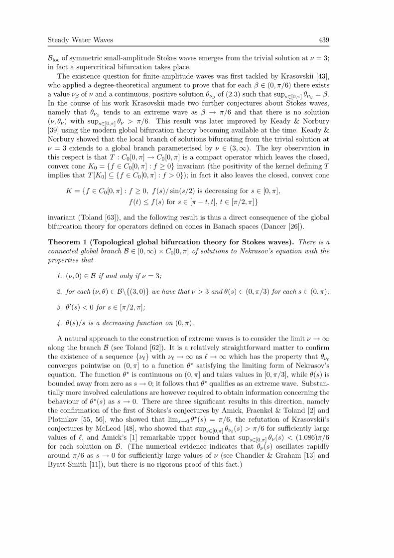
Theorem 1 (Topological global bifurcation theory for Stokes waves). There is aconnected global branch B ∈ [0,∞) × C0[0, π] of solutions to Nekrasov’s equation with theproperties that

1. (ν, 0) ∈ B if and only if ν = 3;

2. for each (ν, θ) ∈ B\{(3, 0)} we have that ν > 3 and θ(s) ∈ (0, π/3) for each s ∈ (0, π);

3. θ′(s) < 0 for s ∈ [π/2, π];

4. θ(s)/s is a decreasing function on (0, π).

A natural approach to the construction of extreme waves is to consider the limit ν → ∞along the branch B (see Toland [62]). It is a relatively straightforward matter to confirmthe existence of a sequence {νℓ} with νℓ → ∞ as ℓ → ∞ which has the property that θνℓ

converges pointwise on (0, π] to a function θ⋆ satisfying the limiting form of Nekrasov’sequation. The function θ⋆ is continuous on (0, π] and takes values in [0, π/3], while θ(s) isbounded away from zero as s→ 0; it follows that θ⋆ qualifies as an extreme wave. Substan-tially more involved calculations are however required to obtain information concerning thebehaviour of θ⋆(s) as s → 0. There are three significant results in this direction, namelythe confirmation of the first of Stokes’s conjectures by Amick, Fraenkel & Toland [2] andPlotnikov [55, 56], who showed that lims→0 θ

⋆(s) = π/6, the refutation of Krasovskii’sconjectures by McLeod [48], who showed that sups∈[0,π] θνℓ

(s) > π/6 for sufficiently largevalues of ℓ, and Amick’s [1] remarkable upper bound that sups∈[0,π] θν(s) < (1.086)π/6for each solution on B. (The numerical evidence indicates that θν(s) oscillates rapidlyaround π/6 as s → 0 for sufficiently large values of ν (see Chandler & Graham [13] andByatt-Smith [11]), but there is no rigorous proof of this fact.)

440 M D Groves

The second of Stokes’s conjectures has recently been confirmed by Plotnikov & Toland[58]. Observe that the integral equation

θ(s) =ρ

π

∫ π

0

sin θ(t)∫ t0 sin θ(u) du

log

∣

∣

∣

∣

∣

sin 12(s+ t)

sin 12(s− t)

∣

∣

∣

∣

∣

dt (2.4)

coincides with Nekrasov’s integral equation for extreme waves when ρ = 1/3 and has theexplicit (and in fact unique) solution θ⋆

1(s) = (π − s)/2 when ρ = 1. Plotnikov & Tolandshowed that equation (2.4) has a continuum C = {(ρ, θ⋆

ρ)}ρ∈[1/3,1] of solutions containingθ⋆1(s) at ρ = 1 and an extreme wave θ⋆

1/3 at ρ = 1/3. The solution θ⋆1 clearly has the

desired convexity property that θ⋆′(s) < 0 for each s ∈ [0, π], and a homotopy argumentasserts that this property is shared by every solution in C, in particular by θ⋆

1/3.

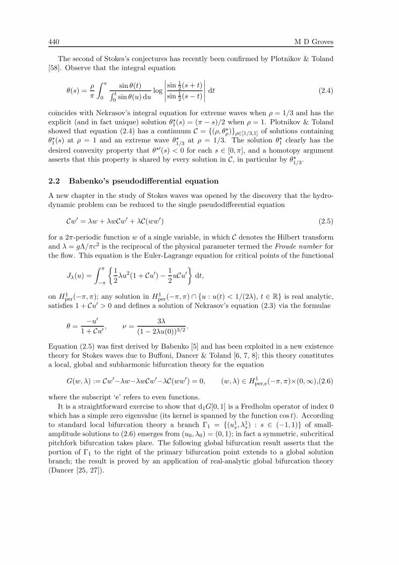
2.2 Babenko’s pseudodifferential equation

A new chapter in the study of Stokes waves was opened by the discovery that the hydro-dynamic problem can be reduced to the single pseudodifferential equation

Cw′ = λw + λwCw′ + λC(ww′) (2.5)

for a 2π-periodic function w of a single variable, in which C denotes the Hilbert transformand λ = gΛ/πc2 is the reciprocal of the physical parameter termed the Froude number forthe flow. This equation is the Euler-Lagrange equation for critical points of the functional

Jλ(u) =

∫ π

−π

{

1

2λu2(1 + Cu′) − 1

2uCu′

}

dt,

on H1per(−π, π); any solution in H1

per(−π, π) ∩ {u : u(t) < 1/(2λ), t ∈ R} is real analytic,satisfies 1 + Cu′ > 0 and defines a solution of Nekrasov’s equation (2.3) via the formulae

θ =−u′

1 + Cu′ , ν =3λ

(1 − 2λu(0))3/2.

Equation (2.5) was first derived by Babenko [5] and has been exploited in a new existencetheory for Stokes waves due to Buffoni, Dancer & Toland [6, 7, 8]; this theory constitutesa local, global and subharmonic bifurcation theory for the equation

G(w, λ) := Cw′−λw−λwCw′−λC(ww′) = 0, (w, λ) ∈ H1per,e(−π, π)×(0,∞),(2.6)

where the subscript ‘e’ refers to even functions.

It is a straightforward exercise to show that d1G[0, 1] is a Fredholm operator of index 0which has a simple zero eigenvalue (its kernel is spanned by the function cos t). Accordingto standard local bifurcation theory a branch Γ1 = {(u1

s, λ1s) : s ∈ (−1, 1)} of small-

amplitude solutions to (2.6) emerges from (u0, λ0) = (0, 1); in fact a symmetric, subcriticalpitchfork bifurcation takes place. The following global bifurcation result asserts that theportion of Γ1 to the right of the primary bifurcation point extends to a global solutionbranch; the result is proved by an application of real-analytic global bifurcation theory(Dancer [25, 27]).

Steady Water Waves 441

Theorem 2 (Real-analytic global bifurcation theory for Stokes waves). The pseu-dodifferential equation (2.6) admits a global solution branch H1 with the following proper-ties.

1. H1 is a continuous graph (us, λs) = h(s), s ∈ (0,∞) with lims→0 h(s) = (1, 0) and0 < λmin ≤ λs ≤ λmax; it may have both self-intersections and cusps.

2. Each solution (us, λs) is 2π-periodic, even, non-increasing on [0, π] and satisfies

maxt∈[−π,π]

us(t) = us(0) < 1/(2λs),

so that it is real analytic.

3. lims→∞ us is an extreme wave.

4. The branch itself consists of a countable number of real analytic arcs

Aj = {u(j)s , (λ(j)

s ) = h(j)(s), s ∈ (s(j)min, s

(j)max)}

which lie in the set S = {(u, λ) : G(u, λ) = 0, d1G[u, λ] is invertible} of regularsolutions and do not self-intersect; the first arc A0 contains the local branch Γ1∩{s >0}. Moreover, at the ‘vertices’ of the arcs which lie in S, the branch admits a locallyanalytic reparameterisation.

Observe thatG(u, λ) in fact has bifurcation points at (0, q) for each q ∈ N, and the abovelocal and global bifurcation results can therefore also be applied at these points to obtainfurther local and global solution branches Γq, Hq, q = 2, 3, . . .; the solutions on on Hq giverise to 2π-periodic solutions whose minimal period is actually 2π/q. A straightforward scal-ing argument shows that (u(q), qλ) is a solution of G(u, λ) = 0, where u(q)(t) = q−1u(qt),whenever (u, λ) is a solution. It follows that {(qλ1

s , w1s(q)) : s ∈ (−1, 1)} is a solution

branch passing through (q, 0), so that Γq is actually obtained from Γ1 using the rescalingformula Γq = {(qλ1

s, w1s(q)) : s ∈ (−δq, δq)}. In fact it is possible to strengthen this result

by showing that, for sufficiently small s, independent of q, the operator ∂2F (qλ1s, w

1s(q)) is

invertible. It follows that Γq can be extended to {(qλ1s, w

1s(q)) : s ∈ (−δ, δ)}, where δ does

not depend upon q, so that each Γq, q ≥ 2 is obtained from Γ1 by scaling in a uniformfashion. It is natural to ask if the rescaled global branch {(qλ1

s, w1s(q)) : s ∈ (0,∞)} likewise

coincides with Hq (see below).Secondary bifurcation means bifurcation of a branch of 2π-periodic solutions from H1.

A result of Kielhofer [40] for real-analytic equations with a gradient structure asserts thata change in the Morse index i(s) of Jλs

at ws⋆ implies a secondary bifurcation from thebranch H1 at h(s⋆) provided that λs is injective in a neighbourhood of s⋆ (that is h(s⋆)is not a turning point of H1). Plotnikov [57] has shown that lim sups→∞ i(s) = ∞, andit follows that there are infinitely many positive values of s (necessarily in h−1(S \ S) atwhich h(s) is a secondary bifurcation point or a turning point. The numerical evidenceindicates that only turning points occur (see Chen & Saffman [14]), but no rigorous proofof this fact is currently available. (Chen & Saffman’s results also predict that secondarybifurcations (of 2qπ-periodic waves) do occur from the branches Hq, q ≥ 2.)

442 M D Groves

Subharmonic bifurcation theory deals with waves which are 2qπ-periodic for some q ≥ 2(and are demonstrably 2π-periodic); the corresponding bifurcation problem is set up in

terms of an operator F (q)(u, λ) and functional J(q)λ (u) which are defined in the same way as

F and Jλ with 2qπ-periodic functions, integration over (−qπ, qπ) and the Hilbert transformCq for 2qπ-periodic functions. Buffoni, Dancer & Toland show that for each sufficiently

large value of q there exists a value of s in h−1(S) at which the Morse index i(q)(s) of J(q)λs

ath(s) changes. Kielhofer’s bifurcation theory shows that a solution of period 2qπ bifurcatesfrom H1 at the point h(s); this solution cannot be 2π-periodic because h(s) ∈ S andtherefore emerges in a subharmonic bifurcation (with minimal period 2qπ if q is prime).

Theorem 3 (Secondary and subharmonic bifurcation theory for Stokes waves).

1. There are infinitely many points on the global branch H1 which are either turningpoints or secondary bifurcation points.

2. For each sufficiently large value of q there exists a point on H1 from which a solutionof period 2qπ emerges in a subharmonic bifurcation.

This result offers several corollaries. Firstly, the global solution branch Hn is notobtained from H1 by rescaling: a subharmonic bifurcation of minimal period 2qπ fromH1 would correspond to a secondary bifurcation (of a 2π-periodic solution) from Hq ata point where dG[u, λ] is invertible. Secondly, no subharmonic bifurcations occur on Γ1,since a subharmonic bifurcation of a solution with minimal period 2qπ from a point of Γ1

would define by rescaling a secondary bifurcation of a 2π-periodic solution from a pointof Γq. Finally, we are able to refute a conjecture made by Levi-Civita, namely that theminimal Froude number πc2/gΛ of a periodic water wave with minimal period 2Λ is notless than unity: the minimal Froude number of a wave with minimal dimensionless period2qπ arising in a subharmonic bifurcation from (us, λs) ∈ H1 is (qλs)

−1, and this numberis bounded above by (qλmin)

−1, which can be made arbitrary small.

2.3 Further results

The above theory for Stokes waves has been extended in several directions. Amick &Toland [3] showed how periodic waves tend to solitary waves (steady waves with a pulse-like profile in the direction of propagation) as the period tends to infinity. In this fashionthey established the existence of supercritical (c2 > gh) solitary waves on water of finitedepth which are symmetric, positive (η > 0) and monotonically decaying on either side ofthe crest. These properties are not restrictions: Craig & Sternberg [21] used the methodof moving planes to show that any supercritical solitary wave is symmetric, positive andmonotonically decaying on either side of its crest. Furthermore, McLeod [47] proved byelementary means that any symmetric, positive solitary wave which decays monotonocallyon either side of its crest is supercritical, while Craig [19] has recently demonstrated thatthere are no solitary waves on water of infinite depth that are single signed (η > 0 orη < 0). A full account of a global bifurcation theory for finite-depth gravity solitary waveswhich is analogous to that for Stokes waves is given by Amick & Toland [4].

There are also extensions of the Stokes-wave theory which include the effects of capil-larity and vorticity. Jones & Toland [38] introduced and studied a version of Nekrasov’s

Steady Water Waves 443

equation for periodic gravity-capillary waves which has become the basis for a large num-ber of analytical and numerical existence theories revealing a much more complex localand global bifurcation picture than that for pure gravity waves. A comprehensive survey ofcurrent results in this area is given by Okamoto & Shoji [53]. The mathematical problemfor rotational Stokes waves is rather different. A velocity potential is not available andthe stream function Ψ (which is again even and 2Λ-periodic in x) satisfies the semilinearequation

−∇Ψ = F (Ψ) in Dη

together with the nonlinear boundary conditions (2.1) and asymptotic condition ∇Ψ →(0,−c) as y → −∞ (uniformly in x); here the vorticity function F specifies the distributionof vorticity in the flow.

The fluid domain of a rotational wave motion satisfying Ψy < 0 can be convenientlymapped to the upper half-plane by interchanging the roles of Ψ and y as dependentand independent variables, so that y = y(x,Ψ) in {(x,Ψ) : Ψ > 0}. Carrying out thistransformation, one finds that y satisfies a quasilinear elliptic equation in the upper half-plane and a fully nonlinear boundary condition on the real axis, and the analysis of thisboundary-value problem is clearly more involved that that of its irrotational counterpart,where helpful re-formulations such as Nekrasov’s or Babenko’s equation can be exploited.Nevertheless a global existence theory for a general class of vorticity functions has recentlybeen presented by Constantin & Strauss [17, 18] (in fact for the finite-depth case). Theirresult is the rotational counterpart of Keady & Norbury’s theory for irrotational Stokeswaves: degree-theoretical methods demonstrate that there is a connected global solutionbranch consisting of symmetric waves whose free-surface profile strictly decreases betweentheir one crest and one trough in each period. Each wave motion satisfies Ψy < 0 and thereis a sequence of solutions (ηn,Ψn) such that max(x,y)∈Dη

Ψny(x, y) → 0. A summary ofprevious work on rotational Stokes waves is also presented in this reference, and Constantin& Escher [16] have shown that large classes of such waves are necessarily symmetric.

3 Spatial dynamics

The phrase ‘spatial dynamics’ refers to an approach where a system of partial differentialequations governing a physical problem is formulated as a (typically ill-posed) evolutionaryequation

uξ = L(u) +N(u), (3.1)

in which an unbounded spatial coordinate plays the role of the time-like variable ξ. Themethod, which was introduced by Kirchgassner [41], has become the basis for a wide rangeof problems in the applied sciences and has proved particularly fruitful in the study of localbifurcation phenomena for two-dimensional steady water waves. This physical problemhas one bounded or semi-bounded coordinate, namely the vertical direction; by contrastno restriction is placed upon the behaviour of the waves in the horizontal direction, and sothis coordinate qualifies as ‘time-like’. We study the problem using spatial dynamics byformulating it as an evolutionary system of the form (3.1), where ξ is the horizontal spatialcoordinate, in an infinite-dimensional phase space consisting of functions of the vertical

444 M D Groves

coordinate. This task is readily accomplished in Levi-Civita’s formulation, where Φ ∈ R

and Ψ ∈ (−∞, 0) are respectively the horizontal and vertical coordinates. Introducing thenew variable γ = ρ|Ψ=1, we find from (2.2) and the Cauchy-Riemann equations for ρ andσ that

ρΦ = σy, (3.2)

σΦ = −ρy, (3.3)

γΦ =g

c3e−3γ sinσ|Ψ=1 (3.4)

with the boundary conditions that ρ, σ → 0 as Ψ → −∞ and γ = ρ|Ψ=1. Equations(3.2)–(3.4) constitute an evolutionary equation for the variable u = (ρ, σ, γ) in the phasespace {(ρ, σ, γ) ∈ L2(−∞, 0)×L2(−∞, 0)×R}, where the domain of the vector field on theright-hand side is {(ρ, σ, γ) ∈ H1(−∞, 0)×H1(−∞, 0)×R : γ = ρ|y=1}. Spatial dynamicsformulations for the finite-depth case and for capillary-gravity steady waves in a finite- orinfinite-depth setting can similarly be obtained from the Levi-Civita coordinates for thoseproblems, and in fact a host of different choices of variables is available (see Groves &Toland [33] for a choice which is closely connected to the original physical variables andhas proved extremely useful in existence theories due to its favourable functional-analyticaspects).

The methods used to find solutions of (3.1) depend heavily upon the characteristics ofthe vector field appearing in the equation, which are in turn determined by the particularproblem being studied. One particularly useful technique is known as centre-manifoldreduction. It is well known that a finite-dimensional dynamical system whose linear parthas purely imaginary eigenvalues admits an invariant manifold called the centre mani-fold which contains all its small, bounded solutions; the dimension of the centre manifoldis given by the number of purely imaginary eigenvalues (e.g. see Vanderbauwhede [65]).Under certain additional hypotheses this result also holds for infinite-dimensional evolu-tionary systems whose linear part has a finite number of purely imaginary eigenvalues.In these circumstances it is therefore possible to show that the original problem is lo-cally equivalent to a system of ordinary differential equations whose solution set can, intheory, be analysed. This reduction procedure is explained in detail by Mielke [49] andVanderbauwhede & Iooss [66] (see in particular §§4–5 in the latter reference for introduc-tory examples and applications), and is applicable to the two-dimensional gravity-capillarywater-wave problem for fluid of finite depth.

An important aspect of the centre-manifold reduction procedure is the fact that itpreserves symmetries of the initial evolutionary equation. The spatial dynamics formu-lation of a conservative problem typically admits a Hamiltonian structure, while that ofan isotropic physical problem is typically reversible, and this Hamiltonian structure orreversibility is inherited by the reduced system on a centre manifold. Other discrete orcontinuous symmetries of the original physical problem are likewise reflected in symme-tries of the reduced vector field. This feature can be exploited in existence theories forwater waves: since the physical problem is conservative and isotropic, its spatial dynamicsformulation is Hamiltonian and reversible, and the reduced system on a centre manifoldis a reversible Hamiltonian system with finitely many degrees of freedom.

Steady Water Waves 445

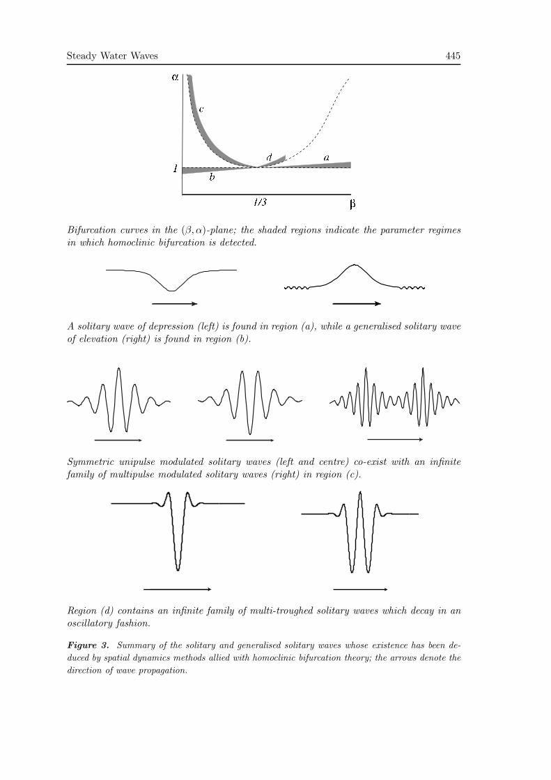
Bifurcation curves in the (β, α)-plane; the shaded regions indicate the parameter regimesin which homoclinic bifurcation is detected.

A solitary wave of depression (left) is found in region (a), while a generalised solitary waveof elevation (right) is found in region (b).

Symmetric unipulse modulated solitary waves (left and centre) co-exist with an infinitefamily of multipulse modulated solitary waves (right) in region (c).

Region (d) contains an infinite family of multi-troughed solitary waves which decay in anoscillatory fashion.

Figure 3. Summary of the solitary and generalised solitary waves whose existence has been de-

duced by spatial dynamics methods allied with homoclinic bifurcation theory; the arrows denote the

direction of wave propagation.

446 M D Groves

Bifurcation phenomena obtained by varying a parameter can also be captured by thecentre-manifold reduction procedure. A bifurcation parameter ǫmay be introduced by per-turbing physical parameters present in the problem around fixed reference values, and thereduction procedure delivers an ǫ-dependent manifold which captures the small-amplitudedynamics for small values of this parameter; the manifold is a true centre manifold atcriticality (ǫ = 0), so that its dimension is the number of purely imaginary eigenvaluesof the relevant linear operator at ǫ = 0. The reduction procedure is therefore especiallyhelpful in detecting bifurcations which are associated with a change in the number ofpurely imaginary eigenvalues. Kirchgassner [42, Fig. 1] showed that there are four criticalcurves in the (β, α)-parameter plane at which the number of purely imaginary eigenvalueschanges, and in fact each of these regions is associated with homoclinic bifurcation, wheresolutions of the reduced system which are asymptotically zero or periodic bifurcate fromthe trivial solution (see below). The parameters in question here are defined by β = T/ch2

and α = c2/gh, and Figure 3 illustrates the regions of (β, α)-parameter space in whichhomoclinic bifurcation takes place.

P

Q

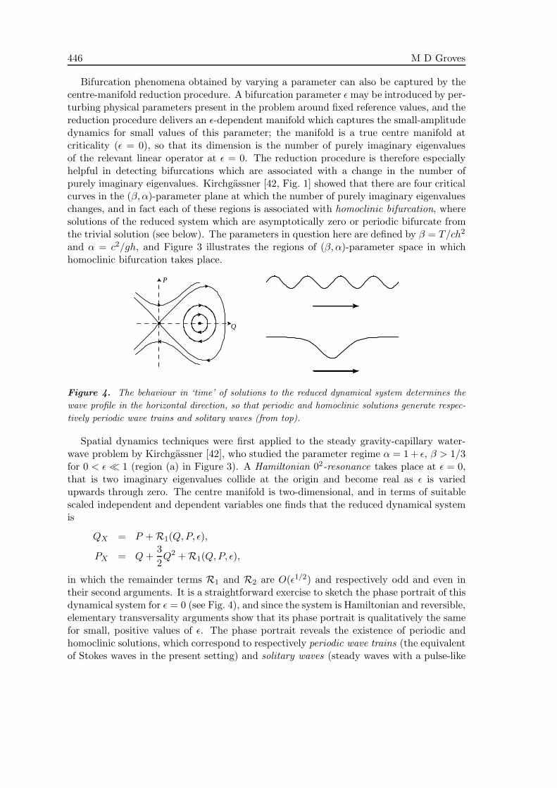
Figure 4. The behaviour in ‘time’ of solutions to the reduced dynamical system determines the

wave profile in the horizontal direction, so that periodic and homoclinic solutions generate respec-

tively periodic wave trains and solitary waves (from top).

Spatial dynamics techniques were first applied to the steady gravity-capillary water-wave problem by Kirchgassner [42], who studied the parameter regime α = 1 + ǫ, β > 1/3for 0 < ǫ ≪ 1 (region (a) in Figure 3). A Hamiltonian 02-resonance takes place at ǫ = 0,that is two imaginary eigenvalues collide at the origin and become real as ǫ is variedupwards through zero. The centre manifold is two-dimensional, and in terms of suitablescaled independent and dependent variables one finds that the reduced dynamical systemis

QX = P + R1(Q,P, ǫ),

PX = Q+3

2Q2 + R1(Q,P, ǫ),

in which the remainder terms R1 and R2 are O(ǫ1/2) and respectively odd and even intheir second arguments. It is a straightforward exercise to sketch the phase portrait of thisdynamical system for ǫ = 0 (see Fig. 4), and since the system is Hamiltonian and reversible,elementary transversality arguments show that its phase portrait is qualitatively the samefor small, positive values of ǫ. The phase portrait reveals the existence of periodic andhomoclinic solutions, which correspond to respectively periodic wave trains (the equivalentof Stokes waves in the present setting) and solitary waves (steady waves with a pulse-like

Steady Water Waves 447

profile in the direction of propagation). Further qualitative details of the correspondingwater waves are obtained by tracing back the various changes of coordinates; one finds forexample that the homoclinic solution in this parameter regime yields to a solitary wave ofdepression.

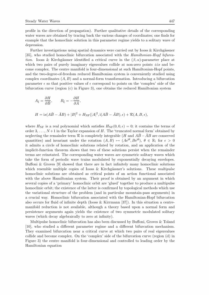
Further investigations using spatial dynamics were carried out by Iooss & Kirchgassner[35], who studied homoclinic bifurcation associated with the Hamiltonian-Hopf bifurca-tion. Iooss & Kirchgassner identified a critical curve in the (β, α)-parameter place atwhich two pairs of purely imaginary eigenvalues collide at non-zero points ±is and be-come complex. The centre manifold is four-dimensional at such Hamiltonian-Hopf points,and the two-degree-of-freedom reduced Hamiltonian system is conveniently studied usingcomplex coordinates (A,B) and a normal-form transformation. Introducing a bifurcationparameter ǫ so that positive values of ǫ correspond to points on the ‘complex’ side of thebifurcation curve (region (c) in Figure 3), one obtains the reduced Hamiltonian system

Aξ =∂H

∂B, Bξ = −∂H

∂A,

H = is(AB − AB) + |B|2 +HNF(|A|2, i(AB − AB), ǫ) + R(A,B, ǫ),

where HNF is a real polynomial which satisfies HNF(0, 0, ǫ) = 0; it contains the terms oforder 3, . . . , N+1 in the Taylor expansion of H. The ‘truncated normal form’ obtained byneglecting the remainder term R is completely integrable (H and AB− AB are conservedquantities) and invariant under the rotation (A,B) 7→ (Aeiθ, Beiθ), θ ∈ R; for ǫ > 0it admits a circle of homoclinic solutions related by rotation, and an application of theimplicit-function theorem shows that two of these solutions persist when the remainderterms are reinstated. The corresponding water waves are symmetric solitary waves whichtake the form of periodic wave trains modulated by exponentially decaying envelopes.Buffoni & Groves [9] showed that there are in fact infinitely many homoclinic solutionswhich resemble multiple copies of Iooss & Kirchgassner’s solutions. These multipulsehomoclinic solutions are obtained as critical points of an action functional associatedwith the above Hamiltonian system. Their proof is obtained by an argument in whichseveral copies of a ‘primary’ homoclinic orbit are ‘glued’ together to produce a multipulsehomoclinic orbit; the existence of the latter is confirmed by topological methods which usethe variational structure of the problem (and in particular mountain-pass arguments) ina crucial way. Homoclinic bifurcation associated with the Hamiltonian-Hopf bifurcationalso occurs for fluid of infinite depth (Iooss & Kirrmann [37]). In this situation a centre-manifold reduction is not available, although a theory based upon a normal form andpersistence arguments again yields the existence of two symmetric modulated solitarywaves (which decay algebraically to zero at infinity).

Multipulse homoclinic bifurcation has also been discussed by Buffoni, Groves & Toland[10], who studied a different parameter regime and a different bifurcation mechanism.They examined bifurcation near a critical curve at which two pairs of real eigenvaluescollide and become complex. On the ‘complex’ side of the bifurcation curve (region (d) inFigure 3) the centre manifold is four-dimensional and controlled to leading order by theHamiltonian equation

448 M D Groves

u′′′′ + (−2 + ǫ)u′′ + u− u2 = 0, 0 < ǫ≪ 1.

This equation has a transverse homoclinic orbit (an orbit arising due to a transverse in-tersection of the two-dimensional stable and unstable manifolds of the zero equilibrium inthe zero energy surface), and hence exhibits chaotic behaviour: there is a Smale-horseshoestructure in its solution set (Devaney [28]). It consequently has an infinite family of multi-pulse homoclinic solutions; the corresponding water waves are solitary waves of depressionwith 2, 3, 4, . . . large troughs separated by 2, 3, . . . small oscillations, and their oscillatorytails decay exponentially to zero.

A different homoclinic bifurcation phenomenon was discovered by Iooss & Kirchgassner[36] in the parameter regime α = 1 + ǫ, β > 1/3 for 0 < ǫ ≪ 1 (region (b) in Figure 3).A Hamiltonian 02iω resonance takes place at ǫ = 0, that is two imaginary eigenvaluescollide at the origin and become real as ǫ is varied downwards through zero, while a sec-ond pair of eigenvalues remains on the imaginary axis. The reduction procedure yields atwo-degree-of-freedom Hamiltonian system, to which Iooss & Kirchgassner applied normal-form techniques. At each order the ‘truncated normal form’ admits two invariant planeswhich contain respectively periodic orbits circling the origin and a homoclinic orbit con-necting the origin with itself. The persistence question for this homoclinic orbit is howeverdifficult to settle because of the geometry of the phase space near the origin: the stableand unstable manifolds are both one-dimensional, and the existence of a homoclinic orbitwould require these manifolds to intersect in the three-dimensional zero energy surface.A similar argument shows that homoclinic connections to periodic orbits are rather to beexpected, and Iooss & Kirchgassner indeed show that there is a family of such homoclinicorbits parameterised by the amplitude of the periodic solutions at infinity; this amplitudeis subject to a lower bound which is algebraically small in the bifurcation parameter. Thecorresponding water waves are called generalised solitary waves; their pulse-like profiledecays to a periodic ripple at infinity.This result has been extended by several authors,notably by Lombardi [45], who has shown that the lower bound on the amplitude of theperiodic ripples at infinity can in fact be made exponentially small in the bifurcation pa-rameter. It is still an open question whether genuine solitary waves exist in this parameterregime, although Sun [61] has recently proved that they do not exist for values of β close to1/3 and there is strong numerical evidence that the same is true for all values of β < 1/3(Champneys et al [12]).

4 Three-dimensional steady waves

The last five years have seen a wealth of new existence results for the previously almostuntouched three-dimensional steady gravity-capillary water-wave problem. They are allvariational in nature, but can be divided into two categories. The mathematical corner-stone of the first is a variational Lyapunov-Schmidt method, while the second consistsof an extension of the spatial dynamics methods described in Section 3 above. Theyyield respectively doubly periodic surface waves and a range of spatially unbounded wavepatterns.

Steady Water Waves 449

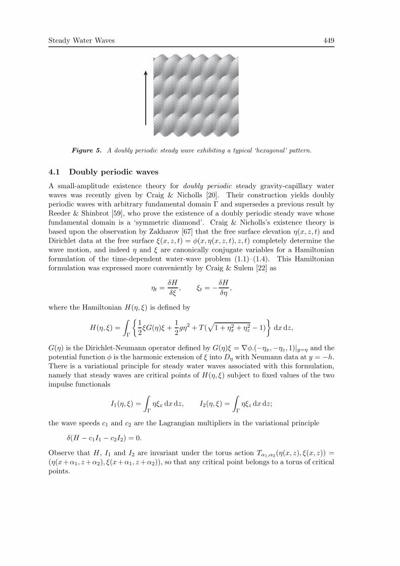
Figure 5. A doubly periodic steady wave exhibiting a typical ‘hexagonal’ pattern.

4.1 Doubly periodic waves

A small-amplitude existence theory for doubly periodic steady gravity-capillary waterwaves was recently given by Craig & Nicholls [20]. Their construction yields doublyperiodic waves with arbitrary fundamental domain Γ and supersedes a previous result byReeder & Shinbrot [59], who prove the existence of a doubly periodic steady wave whosefundamental domain is a ‘symmetric diamond’. Craig & Nicholls’s existence theory isbased upon the observation by Zakharov [67] that the free surface elevation η(x, z, t) andDirichlet data at the free surface ξ(x, z, t) = φ(x, η(x, z, t), z, t) completely determine thewave motion, and indeed η and ξ are canonically conjugate variables for a Hamiltonianformulation of the time-dependent water-wave problem (1.1)–(1.4). This Hamiltonianformulation was expressed more conveniently by Craig & Sulem [22] as

ηt =δH

δξ, ξt = −δH

δη,

where the Hamiltonian H(η, ξ) is defined by

H(η, ξ) =

∫

Γ

{

1

2ξG(η)ξ +

1

2gη2 + T (

√

1 + η2x + η2

z − 1)

}

dxdz,

G(η) is the Dirichlet-Neumann operator defined by G(η)ξ = ∇φ.(−ηx,−ηz, 1)|y=η and thepotential function φ is the harmonic extension of ξ into Dη with Neumann data at y = −h.There is a variational principle for steady water waves associated with this formulation,namely that steady waves are critical points of H(η, ξ) subject to fixed values of the twoimpulse functionals

I1(η, ξ) =

∫

Γηξx dxdz, I2(η, ξ) =

∫

Γηξz dxdz;

the wave speeds c1 and c2 are the Lagrangian multipliers in the variational principle

δ(H − c1I1 − c2I2) = 0.

Observe that H, I1 and I2 are invariant under the torus action Tα1,α2(η(x, z), ξ(x, z)) =

(η(x+α1, z+α2), ξ(x+α1, z+α2)), so that any critical point belongs to a torus of criticalpoints.

450 M D Groves

The above variational principle does not appear to be amenable to the direct methodsof the calculus of variations in any reasonable function space; its framework is howeveranalogous to the situation encountered in the proof of the Lyapunov centre theorem byMoser [50]. There one seeks periodic solutions of a finite-dimensional Hamiltonian systemnear an elliptic equilibrium. Such solutions are characterised as critical points of an actionfunctional subject to fixed values of the averaged Hamiltonian; the unknown period is theLagrange multiplier and all critical points are members of a sphere of critical points dueto autonomy. This variational principle is also not amenable to the direct methods, butnevertheless one can use the Lyapunov-Schmidt method to reduce Hamilton’s equations toa finite-dimensional system of bifurcation equations, solutions of which are critical pointsof a corresponding reduced variational principle. Craig & Nicholls apply this strategy tothe above variational principle for steady water waves.

The crucial ingredients are the specification of the function space in which the equationsδ(H − c1I1 − c2I2) = 0 are to be considered, for which purpose a precise description of themapping properties of G(η) in appropriate Sobolev spaces is required, and a proof thatthe kernel of the linearised equations is finite-dimensional. This fact is readily understoodin terms of the physics of the underlying problem. Representing doubly periodic functionsas Fourier series, one can show that a zero eigenvalue occurs whenever the wave numberk = (k1, k2) and wave velocity c = (c1, c2) satisfy the classical dispersion relation

∆(c, k) = (g + T |k|2)|k| tanh(|k|h) − (c.k)2 = 0.

For fixed c0, each solution k0 of ∆(c0, k) = 0 leads to a zero eigenvalue, and clearlysuch values of k occur in pairs ±k0. The nullity of the linear operator is therefore twicethe number N of solutions {k1, . . . , kN} of ∆(c0, k) = 0 which are normalised such thatk.c0 = 0, and one easily finds that 2 ≤ N < ∞. (The fact that T > 0 is crucialin this respect; in the case T = 0 (gravity waves) the kernel of the linear operator isinfinite-dimensional, and existence theories for doubly periodic gravity waves are thereforelikely to encounter small-divisor problems. This observation has already been made in ashort note by Plotnikov [54], and although Plotnikov gave a sketch of an existence prooffor doubly periodic steady gravity waves using superconvergence methods this problemremains essentially open.)

Having applied Moser’s reduction technique, we arrive at the reduced variational princi-ple of finding the critical points of a smooth functional H on a two-codimensional compactsubmanifold S of 2N -dimensional real space; the problem is equivariant with respect to atorus action Tα. The fact that the quadratic part of the original Hamiltonian H is positivedefinite implies that S is given geometrically as the intersection of two ellipsoids, and wecan this feature to conclude the existence of periodic orbits without considering the non-linear problem in detail. When N = 2 the set S is homeomorphic to a two-dimensionaltorus and the orbit under Tα of any point of S is the whole of S, so that H|S is constantand has one Tα-equivariant critical point. The ‘symmetric diamond’ solution of Reederand Shinbrot is a special case with k1 = (κ, ℓ), k2 = (κ,−ℓ), κ 6= ℓ. When N > 2 theset S is homeomorphic to the product of two spheres, and it follows that there are atleast indTαS + 1 distinct Tα-equivariant critical points of H on S, where indTαS is a Tα-equivariant cohomological index of S. Craig & Nicholls show that it is always possible tochoose the index so that indTαS = N − 2.

Steady Water Waves 451

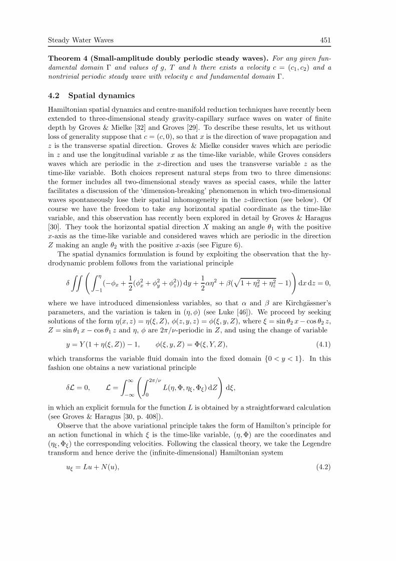
Theorem 4 (Small-amplitude doubly periodic steady waves). For any given fun-damental domain Γ and values of g, T and h there exists a velocity c = (c1, c2) and anontrivial periodic steady wave with velocity c and fundamental domain Γ.

4.2 Spatial dynamics

Hamiltonian spatial dynamics and centre-manifold reduction techniques have recently beenextended to three-dimensional steady gravity-capillary surface waves on water of finitedepth by Groves & Mielke [32] and Groves [29]. To describe these results, let us withoutloss of generality suppose that c = (c, 0), so that x is the direction of wave propagation andz is the transverse spatial direction. Groves & Mielke consider waves which are periodicin z and use the longitudinal variable x as the time-like variable, while Groves considerswaves which are periodic in the x-direction and uses the transverse variable z as thetime-like variable. Both choices represent natural steps from two to three dimensions:the former includes all two-dimensional steady waves as special cases, while the latterfacilitates a discussion of the ‘dimension-breaking’ phenomenon in which two-dimensionalwaves spontaneously lose their spatial inhomogeneity in the z-direction (see below). Ofcourse we have the freedom to take any horizontal spatial coordinate as the time-likevariable, and this observation has recently been explored in detail by Groves & Haragus[30]. They took the horizontal spatial direction X making an angle θ1 with the positivex-axis as the time-like variable and considered waves which are periodic in the directionZ making an angle θ2 with the positive x-axis (see Figure 6).

The spatial dynamics formulation is found by exploiting the observation that the hy-drodynamic problem follows from the variational principle

δ

∫∫

(

∫ η

−1(−φx +

1

2(φ2

x + φ2y + φ2

z)) dy +1

2αη2 + β(

√

1 + η2x + η2

z − 1)

)

dxdz = 0,

where we have introduced dimensionless variables, so that α and β are Kirchgassner’sparameters, and the variation is taken in (η, φ) (see Luke [46]). We proceed by seekingsolutions of the form η(x, z) = η(ξ, Z), φ(z, y, z) = φ(ξ, y, Z), where ξ = sin θ2 x− cos θ2 z,Z = sin θ1 x− cos θ1 z and η, φ are 2π/ν-periodic in Z, and using the change of variable

y = Y (1 + η(ξ, Z)) − 1, φ(ξ, y, Z) = Φ(ξ, Y, Z), (4.1)

which transforms the variable fluid domain into the fixed domain {0 < y < 1}. In thisfashion one obtains a new variational principle

δL = 0, L =

∫ ∞

−∞

(

∫ 2π/ν

0L(η,Φ, ηξ ,Φξ) dZ

)

dξ,

in which an explicit formula for the function L is obtained by a straightforward calculation(see Groves & Haragus [30, p. 408]).

Observe that the above variational principle takes the form of Hamilton’s principle foran action functional in which ξ is the time-like variable, (η,Φ) are the coordinates and(ηξ,Φξ) the corresponding velocities. Following the classical theory, we take the Legendretransform and hence derive the (infinite-dimensional) Hamiltonian system

uξ = Lu+N(u), (4.2)

452 M D Groves

z

x

Z ξ

θθ

1

2

Direction of

wave propagation

'Time-like'

horizontal coordinate'Space-like'

horizontal coordinate

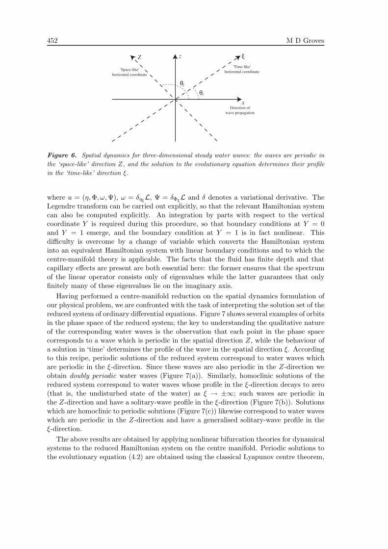
Figure 6. Spatial dynamics for three-dimensional steady water waves: the waves are periodic in

the ‘space-like’ direction Z, and the solution to the evolutionary equation determines their profile

in the ‘time-like’ direction ξ.

where u = (η,Φ, ω,Ψ), ω = δηξL, Ψ = δΦξ

L and δ denotes a variational derivative. TheLegendre transform can be carried out explicitly, so that the relevant Hamiltonian systemcan also be computed explicitly. An integration by parts with respect to the verticalcoordinate Y is required during this procedure, so that boundary conditions at Y = 0and Y = 1 emerge, and the boundary condition at Y = 1 is in fact nonlinear. Thisdifficulty is overcome by a change of variable which converts the Hamiltonian systeminto an equivalent Hamiltonian system with linear boundary conditions and to which thecentre-manifold theory is applicable. The facts that the fluid has finite depth and thatcapillary effects are present are both essential here: the former ensures that the spectrumof the linear operator consists only of eigenvalues while the latter guarantees that onlyfinitely many of these eigenvalues lie on the imaginary axis.

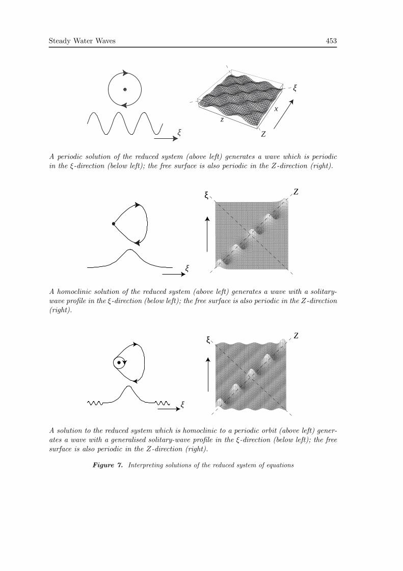
Having performed a centre-manifold reduction on the spatial dynamics formulation ofour physical problem, we are confronted with the task of interpreting the solution set of thereduced system of ordinary differential equations. Figure 7 shows several examples of orbitsin the phase space of the reduced system; the key to understanding the qualitative natureof the corresponding water waves is the observation that each point in the phase spacecorresponds to a wave which is periodic in the spatial direction Z, while the behaviour ofa solution in ‘time’ determines the profile of the wave in the spatial direction ξ. Accordingto this recipe, periodic solutions of the reduced system correspond to water waves whichare periodic in the ξ-direction. Since these waves are also periodic in the Z-direction weobtain doubly periodic water waves (Figure 7(a)). Similarly, homoclinic solutions of thereduced system correspond to water waves whose profile in the ξ-direction decays to zero(that is, the undisturbed state of the water) as ξ → ±∞; such waves are periodic inthe Z-direction and have a solitary-wave profile in the ξ-direction (Figure 7(b)). Solutionswhich are homoclinic to periodic solutions (Figure 7(c)) likewise correspond to water waveswhich are periodic in the Z-direction and have a generalised solitary-wave profile in theξ-direction.

The above results are obtained by applying nonlinear bifurcation theories for dynamicalsystems to the reduced Hamiltonian system on the centre manifold. Periodic solutions tothe evolutionary equation (4.2) are obtained using the classical Lyapunov centre theorem,

Steady Water Waves 453

xz

Zξ

ξ

A periodic solution of the reduced system (above left) generates a wave which is periodicin the ξ-direction (below left); the free surface is also periodic in the Z-direction (right).

ξ Z

ξ

A homoclinic solution of the reduced system (above left) generates a wave with a solitary-wave profile in the ξ-direction (below left); the free surface is also periodic in the Z-direction(right).

ξ Z

ξ

A solution to the reduced system which is homoclinic to a periodic orbit (above left) gener-ates a wave with a generalised solitary-wave profile in the ξ-direction (below left); the freesurface is also periodic in the Z-direction (right).

Figure 7. Interpreting solutions of the reduced system of equations

454 M D Groves

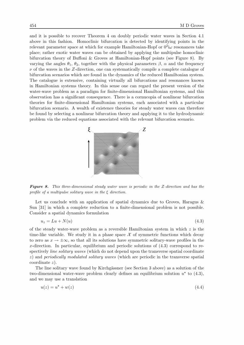
and it is possible to recover Theorem 4 on doubly periodic water waves in Section 4.1above in this fashion. Homoclinic bifurcation is detected by identifying points in therelevant parameter space at which for example Hamiltonian-Hopf or 02iω resonances takeplace; rather exotic water waves can be obtained by applying the multipulse homoclinicbifurcation theory of Buffoni & Groves at Hamiltonian-Hopf points (see Figure 8). Byvarying the angles θ1, θ2, together with the physical parameters β, α and the frequencyν of the waves in the Z-direction, one can systematically compile a complete catalogue ofbifurcation scenarios which are found in the dynamics of the reduced Hamiltonian system.The catalogue is extensive, containing virtually all bifurcations and resonances knownin Hamiltonian systems theory. In this sense one can regard the present version of thewater-wave problem as a paradigm for finite-dimensional Hamiltonian systems, and thisobservation has a significant consequence. There is a cornucopia of nonlinear bifurcationtheories for finite-dimensional Hamiltonian systems, each associated with a particularbifurcation scenario. A wealth of existence theories for steady water waves can thereforebe found by selecting a nonlinear bifurcation theory and applying it to the hydrodynamicproblem via the reduced equations associated with the relevant bifurcation scenario.

ξ Z

Figure 8. This three-dimensional steady water wave is periodic in the Z-direction and has the

profile of a multipulse solitary wave in the ξ direction.

Let us conclude with an application of spatial dynamics due to Groves, Haragus &Sun [31] in which a complete reduction to a finite-dimensional problem is not possible.Consider a spatial dynamics formulation

uz = Lu+N(u) (4.3)

of the steady water-wave problem as a reversible Hamiltonian system in which z is thetime-like variable. We study it in a phase space X of symmetric functions which decayto zero as x → ±∞, so that all its solutions have symmetric solitary-wave profiles in thex-direction. In particular, equilibrium and periodic solutions of (4.3) correspond to re-spectively line solitary waves (which do not depend upon the transverse spatial coordinatez) and periodically modulated solitary waves (which are periodic in the transverse spatialcoordinate z).

The line solitary wave found by Kirchgassner (see Section 3 above) as a solution of thetwo-dimensional water-wave problem clearly defines an equilibrium solution u⋆ to (4.3),and we may use a translation

u(z) = u⋆ + w(z) (4.4)

Steady Water Waves 455

to obtain the new Hamiltonian system

wz = L⋆w +N⋆(w). (4.5)

The spectrum of L⋆ consists of two simple imaginary eigenvalues ±ikǫ, where kǫ is O(ǫ),together with essential spectrum along the whole of the real axis. The presence of this es-sential spectrum rules out the use of centre-manifold theory which would, together with anapplication of the Lyapunov centre theorem to the reduced Hamiltonian system, yield theexistence of a family of small-amplitude periodic solutions to (4.5). Iooss [34] has howeverrecently established a version of the Lyapunov centre theorem for reversible systems ininfinite-dimensional settings with spectrum of this kind (for which the nonresonance condi-tion on the eigenvalues is violated at the origin due to the presence of essential spectrum).Groves, Haragus & Sun verified that the conditions in Iooss’s theorem are satisfied byequation (4.5), which therefore has a family of periodic solutions with frequency of O(ǫ); afamily of periodically modulated solitary water waves is obtained using formula (4.4). Theresult of this analysis is stated in Theorem 5 below; the line solitary wave is sketched inFigure 9 together with a typical member of the family of periodically modulated solitarywaves.

Figure 9. The periodically modulated solitary wave on the right emerges from the line solitary

wave on the left in a dimension-breaking bifurcation. The arrow indicates the direction of wave

propagation.

Theorem 5 (Dimension-breaking phenomenon). Suppose that β > 1/3 and α = 1+ǫ.There exists a positive constant ω0 in the interval (0, 1/(4(β − 1/3))1/2) and, for eachsufficiently small value of ǫ, a small neighbourhood Nǫ of the origin in R such that thefollowing statements hold.

1. The hydrodynamic problem admits a line solitary-wave solution (η⋆(x), φ⋆(x, y)),where

η⋆(x) = −ǫ sech2

(

ǫ1/2x

2(β − 1/3)1/2

)

+O(ǫ2)

and η⋆(−x) = η⋆(x) for all x ∈ R. The quantities η⋆ and φ⋆ decay exponentially tozero with exponential rate ǫ1/2r⋆ as x → ±∞, where r⋆ is any real positive numberstrictly less than (4(β − 1/3))−1/2.

456 M D Groves

2. A family of periodically modulated solitary waves {(ηa(x, z), φa(x, y, z))}a∈Nǫ emergesfrom the above line solitary wave in a dimension-breaking bifurcation. Here

ηa(x, z) = η⋆(x) + ǫη⋆a(ǫ

1/2x, z),

in which η⋆a(· , ·) has amplitude of O(|a|) and is even in both arguments and periodic

in its second argument with frequency ǫkǫ +O(|a|2); the positive number kǫ satisfies|kǫ − ω0| = O(ǫ1/4).

References

[1] Amick, C. J. 1987 Bounds for water waves. Arch. Rat. Mech. Anal. 99, 91–114.

[2] Amick, C. J., Fraenkel, L. E. & Toland, J. F. 1982 On the Stokes conjecturefor the wave of extreme form. Acta. Math. 148, 193–214.

[3] Amick, C. J. & Toland, J. F. 1981 On periodic water waves and their convergenceto solitary waves in the long-wave limit. Phil. Trans. R. Soc. 303, 633–673.

[4] Amick, C. J. & Toland, J. F. 1981 On solitary waves of finite amplitude. Arch.Rat. Mech. Anal. 76, 9–95.

[5] Babenko, K. I. 1987 Some remarks on the theory of surface waves of finite amplitude.Sov. Math. Dokl. 35, 599–603.

[6] Buffoni, B., Dancer, E. N. & Toland, J. F. 1998 Sur les ondes de Stokes etune conjecture de Levi-Civita. C. R. Acad. Sci. Paris, Ser. 1 326, 1265–1268.

[7] Buffoni, B., Dancer, E. N. & Toland, J. F. 2000 The regularity and localbifurcation of steady periodic water waves. Arch. Rat. Mech. Anal. 152, 207–240.

[8] Buffoni, B., Dancer, E. N. & Toland, J. F. 2000 The sub-harmonic bifurcationof Stokes waves. Arch. Rat. Mech. Anal. 152, 241–271.

[9] Buffoni, B. & Groves, M. D. 1999 A multiplicity result for solitary gravity-capillary waves in deep water via critical-point theory. Arch. Rat. Mech. Anal. 146,183–220.

[10] Buffoni, B., Groves, M. D. & Toland, J. F. 1996 A plethora of solitary gravity-capillary water waves with nearly critical Bond and Froude numbers. Phil. Trans.Roy. Soc. Lond. A 354, 575–607.

[11] Byatt-Smith, J. G. 2001 Numerical solution of Nekrasov’s equation in the boundarylayer near the crest for waves near the maximum height. Stud. Appl. Math. 106, 393–405.

[12] Champneys, A. R., Vanden-Broeck, J.-M. & Lord, G. J. 2002 Do true eleva-tion gravity-capillary solitary waves exist? A numerical investigation. J. Fluid Mech.454, 403–417.

Steady Water Waves 457

[13] Chandler, G. A. & Graham, I. G. 1993 The computation of water waves modelledby Nekrasov’s equation. SIAM J. Numer. Anal. 30, 1041–1065.

[14] Chen, B. & Saffman, P. G. 1980 Numerical evidence for the existence of newtypes of gravity wave of permanent form on deep water. Stud. Appl. Math. 62, 1–21.

[15] Constantin, A. 2001 On the deep water wave motion. J. Phys. A 34, 1405–1417.

[16] Constantin, A. & Escher, J. 2004 Symmetry of steady periodic surface waterwaves with vorticity. J. Fluid Mech. 498, 171–181.

[17] Constantin, A. & Strauss, W. 2002 Exact periodic traveling water waves withvorticity. C. R. Acad. Sci. Paris, Ser. 1 335, 797–800.

[18] Constantin, A. & Strauss, W. 2004 Exact steady periodic water waves withvorticity. Commun. Pure Appl. Math. 57, 481–527.

[19] Craig, W. 2002 Nonexistence of solitary water waves in three dimensions. Phil.Trans. Roy. Soc. Lond. A 360, 2127–2135.

[20] Craig, W. & Nicholls, D. P. 2000 Traveling two and three dimensional capillarygravity water waves. SIAM J. Math. Anal. 32, 323–359.

[21] Craig, W. & Sternberg, P. 1988 Symmetry of solitary waves. Commun. PartialDiff. Eqns. 13, 603–633.

[22] Craig, W. & Sulem, C. 1993 Numerical simulation of gravity waves. J. Comp.Phys. 108, 73–83.

[23] Crapper, G. D. 1957 An exact solution for progressive capillary waves of arbitraryamplitude. J. Fluid Mech. 2, 532–540.

[24] Crapper, G. D. 1976 Exact large amplitude capillary waves on sheets of fluid. J.Fluid Mech. 77, 229–241.

[25] Dancer, E. N. 1973 Bifurcation theory for analytic operators. Proc. Lond. Math.Soc. 26, 359–384.

[26] Dancer, E. N. 1973 Global solution branches for positive mappings. Arch. Rat.Mech. Anal. 52, 181–192.

[27] Dancer, E. N. 1973 Global structure of the solution set of non-linear real-analyticoperators. Proc. Lond. Math. Soc. 27, 747–765.

[28] Devaney, R. L. 1976 Homoclinic orbits in Hamiltonian systems. J. Diff. Eqns. 21,431–438.

[29] Groves, M. D. 2001 An existence theory for three-dimensional periodic travellinggravity-capillary water waves with bounded transverse profiles. Physica D 152–153,395–415.

458 M D Groves

[30] Groves, M. D. & Haragus, M. 2003 A bifurcation theory for three-dimensionaloblique travelling gravity-capillary water waves. J. Nonlinear Sci. 13, 397–447.

[31] Groves, M. D., Haragus, M. & Sun, S.-M. 2002 A dimension-breaking phe-nomenon in the theory of gravity-capillary water waves. Phil. Trans. Roy. Soc. Lond.A 360, 2189–2243.

[32] Groves, M. D. & Mielke, A. 2001 A spatial dynamics approach to three-dimensional gravity-capillary steady water waves. Proc. Roy. Soc. Edin. A 131, 83–136.

[33] Groves, M. D. & Toland, J. F. 1997 On variational formulations for steady waterwaves. Arch. Rat. Mech. Anal. 137, 203–226.

[34] Iooss, G. 1999 Gravity and capillary-gravity periodic travelling waves for two super-posed fluid layers, one being of infinite depth. J. Math. Fluid Mech. 1, 24–63.

[35] Iooss, G. & Kirchgassner, K. 1990 Bifurcation d’ondes solitaires en presenced’une faible tension superficielle. C. R. Acad. Sci. Paris, Ser. 1 311, 265–268.

[36] Iooss, G. & Kirchgassner, K. 1992 Water waves for small surface tension: anapproach via normal form. Proc. Roy. Soc. Edin. A 122, 267–299.

[37] Iooss, G. & Kirrmann, P. 1996 Capillary gravity waves on the free surface of aninviscid fluid of infinite depth. Existence of solitary waves. Arch. Rat. Mech. Anal.136, 1–19.

[38] Jones, M. & Toland, J. F. 1986 Symmetry and the bifurcation of capillary-gravitywaves. Arch. Rat. Mech. Anal. 96, 29–53.

[39] Keady, G. & Norbury, J. 1978 On the existence theory for irrotational waterwaves. Math. Proc. Camb. Phil. Soc. 83, 137–157.

[40] Kielhofer, H. 1988 A bifurcation theorem for potential operators. J. Func. Anal.77, 1–8.

[41] Kirchgassner, K. 1982 Wave solutions of reversible systems and applications. J.Diff. Eqns. 45, 113–127.

[42] Kirchgassner, K. 1988 Nonlinear resonant surface waves and homoclinic bifurca-tion. Adv. Appl. Math. 26, 135–181.

[43] Krasovskii, Y. P. 1961 On the theory of steady-state waves of large amplitude.U.S.S.R. Comp. Math. and Math. Phys. 1, 996–1018.

[44] Levi-Civita, T. 1925 Determination rigoureuse des ondes permanentes d’ampleurfinie. Math. Ann. 93, 264–314.

[45] Lombardi, E. 1997 Orbits homoclinic to exponentially small periodic orbits for aclass of reversible systems. Application to water waves. Arch. Rat. Mech. Anal. 137,227–304.

Steady Water Waves 459

[46] Luke, J. C. 1967 A variational principle for a fluid with a free surface. J. Fluid Mech.27, 395–397.

[47] McLeod, J. B. 1984 The Froude number for solitary waves. Proc. Roy. Soc. Edin.A 97, 193–197.

[48] McLeod, J. B. 1997 Stokes and Krasovskii’s conjectures for the wave of greatestheight. Stud. Appl. Math. 98, 311–334.

[49] Mielke, A. 1991 Hamiltonian and Lagrangian Flows on Center Manifolds. Berlin:Springer-Verlag.

[50] Moser, J. 1976 Periodic orbits near an equilibrium and a theorem by Alan Weinstein.Commun. Pure Appl. Math. 29, 727–747.

[51] Nekrasov, A. I. 1921 On steady waves. Izv. Ivanovo-Voznesensk. Politekhn. In-ta3.

[52] Nekrasov, A. I. 1951 The exact theory of steady waves on the surface of a heavyfluid. Izdat. Akad. Nauk. SSSR, Moscow .

[53] Okamoto, H. & Shoji, M. 2001 The Mathematical Theory of Permanent Progres-sive Water-Waves. Singapore: World Scientific.

[54] Plotnikov, P. I. 1980 Solvability of the problem of spatial gravitational waves onthe surface of an ideal fluid. Sov. Phys. Dokl. 25, 170–171.

[55] Plotnikov, P. I. 1982 A proof of the Stokes conjecture in the theory of surfacewaves. Dinamika Splosh. Sredy 57, 41–76. (English translation Stud. Appl. Math.108, 217–244.)

[56] Plotnikov, P. I. 1983 Justification of the Stokes hypothesis in the theory of surfacewaves. Soviet Phys. Dokl. 28.

[57] Plotnikov, P. I. 1992 Nonuniqueness of solutions of the problem of solitary wavesand bifurcation of critical points of smooth functionals. Math. USSR Izvestiya 38,333–357.

[58] Plotnikov, P. I. & Toland, J. F. 2004 Convexity of Stokes waves of extremeform. Arch. Rat. Mech. Anal. 171, 349–416.

[59] Reeder, J. & Shinbrot, M. 1981 Three dimensional nonlinear wave interaction inwater of constant depth. Nonlinear Analysis TMA 5, 303–323.

[60] Stokes, G. G. 1880 Considerations relative to the greatest height of oscillatoryirrotational waves which can be propogated without change of form. In Mathematicaland Physical Papers, Volume 1 , pages 225–228. Cambridge: C.U.P.

[61] Sun, S. M. 1999 Nonexistence of truly solitary waves with small surface tension.Proc. Roy. Soc. Lond. A 455, 2191–2228.

460 M D Groves

[62] Toland, J. F. 1978 On the existence of a wave of greatest height and Stokes’sconjecture. Proc. Roy. Soc. Lond. A 363, 469–485.

[63] Toland, J. F. 1996 Stokes waves. Topol. Meth. Nonlinear Anal. 7, 1–48.

[64] Toland, J. F. 1999 On the symmetry theory for Stokes waves of finite and infinitedepth. In Monographs and Surveys in Pure and Applied Mathematics 106 — Trendsin Applications of Mathematics to Mechanics (eds. Iooss, G., Gues, O. & Nouri, A.),pages 207–217. Boca Raton, Florida: Chapman & Hall/CRC.

[65] Vanderbauwhede, A. 1989 Centre manifolds, normal forms and elementary bifur-cations. Dynamics Reported 2, 89–169.

[66] Vanderbauwhede, A. & Iooss, G. 1992 Centre manifold theory in infinite dimen-sions. Dynamics Reported 1, 125–163.

[67] Zakharov, V. E. 1968 Stability of periodic waves of finite amplitude on the surfaceof a deep fluid. Zh. Prikl. Mekh. Tekh. Fiz. 9, 86–94. (English translation J. Appl.Mech. Tech. Phys. 9, 190–194.)