Journal of Mathematical Imaging and Vision manuscript No.

Journal of Mathematical Imaging and Vision manuscript No.(will be inserted by the editor)

Image Anomalies: a Review and Synthesis of DetectionMethods

Thibaud Ehret? · Axel Davy? · Jean-Michel Morel · Mauricio Delbracio

Received: date / Accepted: date

Abstract We review the broad variety of methods that

have been proposed for anomaly detection in images.

Most methods found in the literature have in mind a

particular application. Yet we focus on a classification

of the methods based on the structural assumption they

make on the “normal” image, assumed to obey a “back-

ground model”. Five different structural assumptions

emerge for the background model. Our analysis leads

us to reformulate the best representative algorithms in

each class by attaching to them an a-contrario detec-

tion that controls the number of false positives and thus

deriving a uniform detection scheme for all. By combin-

ing the most general structural assumptions expressing

the background’s normality with the proposed generic

statistical detection tool, we end up proposing several

generic algorithms that seem to generalize or reconcilemost methods. We compare the six best representatives

of our proposed classes of algorithms on anomalous im-

ages taken from classic papers on the subject, and on

a synthetic database. Our conclusion hints that it is

? Both authors contributed equally to this work.Work supported by IDEX Paris-Saclay IDI 2016, ANR-11-IDEX-0003-02, ONR grant N00014-17-1-2552, CNES MISSproject, Agencia Nacional de Investigacion e Innovacion(ANII, Uruguay) grant FCE 1 2017 135458, DGA AstridANR-17-ASTR-0013-01, DGA ANR-16-DEFA-0004-01, Pro-gramme ECOS Sud – UdelaR - Paris Descartes U17E04, andMENRT.

Thibaud Ehret · Axel Davy · Jean-Michel MorelCMLA, ENS Cachan, CNRS, Universite Paris-Saclay, 94235Cachan, FranceE-mail: [email protected]: [email protected]

Mauricio DelbracioIIE, Facultad de Ingenierıa, Universidad de la Republica,Uruguay

possible to perform automatic anomaly detection on a

single image.

Keywords Anomaly detection, multiscale, back-

ground modeling, background subtraction, self-

similarity, sparsity, center-surround, hypothesis

testing, p-value, a-contrario assumption, number of

false alarms.

1 Introduction

The automatic detection of anomalous structure in ar-

bitrary images is concerned with the problem of find-

ing non-confirming patterns with respect to the image

normality. This is a challenging problem in computer

vision, since there is no clear and straightforward def-

inition of what is (ab)normal for a given arbitrary im-

age. Automatic anomaly detection has high stakes in

industry, remote sensing and medicine (Figure 1). It

is crucial to be able to handle automatically massive

data to detect for example anomalous masses in mam-

mograms [56, 130], chemical targets in multi-spectral

and hyper-spectral satellite images [5, 40, 124, 129], sea

mines in side-scan sonar images [95], or defects in in-

dustrial monitoring applications [138, 149, 153]. This

detection may be done using any imaging device from

cameras to scanning electron microscopes [20].

Our goal here is to review the broad variety of meth-

ods that have been proposed for this problem in the

realm of image processing. We would like to classify the

methods, but also to decide if some arguably general

anomaly detection framework emerges from the anal-

ysis. This is not obvious: most reviewed methods were

designed for a particular application, even if most claim

some degree of generality.

arX

iv:1

808.

0256

4v2

[cs

.CV

] 3

Jun

201

9

2 Thibaud Ehret? et al.

Yet, all anomaly detection methods make a gen-

eral structural assumption on the “normal” background

that actually characterizes the method. By combining

the most general structural assumptions with statistical

detection tools controlling the number of false alarms,

we shall converge to a few generic algorithms that seem

to generalize or reconcile most methods.

To evaluate our conclusions, we shall compare rep-

resentatives of the main algorithmic classes on classic

and diversified examples. A fair comparison will require

completing them when necessary with a common sta-

tistical decision threshold.

Plan of the paper. In the next subsection 1.1, we make

a first sketch of definition of the problem, define the

main terminology and give the notation for the sta-

tistical framework used throughout the paper. Section

1.2 reviews four anterior reviews and discusses their

methodology. Section 1.3 circumscribes our field of in-

terest by excluding several related but different ques-

tions. In the central Section 2 we propose a classifica-

tion of the anomaly detectors into five classes depend-

ing on the main structural assumption made on the

background model. This section contains the descrip-

tion and analysis of about 50 different methods. This

analysis raises the question of defining a uniform de-

tection scheme for all background structures. Hence, in

Section 3 we incorporate a uniform probabilistic detec-

tion threshold to the most relevant methods spotted in

Section 2. This enables us in Section 4 to build three

comparison protocols for six methods representative of

each class. We finally conclude in Section 5.

1.1 Is there a formal generic framework for the

problem?

Because of the variety of methods proposed, it is virtu-

ally impossible to start with a formal definition of the

problem. Nevertheless, this subsection circumscribes it

and lists the most important terms and concepts recur-

ring in most papers. Each new term will be indicated

in italic.

Our study is limited to image anomalies for obvious

experimental reasons: we need a common playground

to compare methods. Images have a specific geomet-

ric structure and homogeneity which is different from

(say) audio or text. For example, causal anomaly detec-

tors based on predictive methods such as autoregressive

conditional heteroskedasticity (ARCH) models fall out

of our field. (We shall nevertheless study an adaptation

of ARCH to anomaly detection in sonar images.)

Like in the overwhelming majority of reviewed pa-

pers, we assume that anomalies can be detected in and

from a single image, or from an image data set, even

if they do contain anomalies. Learning the background

or “normal” model from images containing anomalies

nevertheless implies that anomalies are small, both in

size and proportion to the processed images, as stated

for example in [106]:

“We consider the problem of detecting points

that are rare within a data set dominated by

the presence of ordinary background points.”

Without loss of generality, we shall evaluate the

methods on single images. It appears that for the over-

whelming majority of considered methods, a single im-

age has enough samples to learn a background model.

As a matter of fact, many methods are proceeded lo-

cally in the image or in a feature space, which implies

that the background model for each detection test is

learned only on a well chosen portion of the image or

of the samples. Nevertheless for industrial applications,

using a fixed database representative of anomaly-free

images can help reduce false alarms and computation

time, and studied methods can generally be adapted to

this scenario. All methods extract vector samples from

the images, either hyperspectral pixels generally denoted

by xi, xj , xr · · · , or image patches, namely sub-images

of the image u with moderate size, typically from 2× 2

to 16 × 16, generally denoted by pi, pj , qr, qs, · · · . The

vector samples may be also obtained as a feature vector

obtained by a linear transform (e.g. wavelet coefficients)

or by a linear or nonlinear coordinate transform such

as, PCA, kernel PCA or diffusion maps, or as coordi-

nates in a sparse dictionary. We denote the resulting

vector representing a sample by xi, yi, · · · or pi, qi, · · · .From these samples taken from an image (or from a

collection of images), all considered anomaly detection

methods estimate (implicitly or explicitly) a background

model, also known as model of normal samples. The

goal of the background model is to provide for each

sample a measure of its rareness. This rarity measure is

generally called a saliency map. It requires an empirical

threshold to decide which pixels or patches are salient

enough to be called anomalies. If the background model

is stochastic, a probability of false alarm or p-value can

be associated with each sample, under the assumption

that it obeys the background model.

The methods will be mainly characterized by the

structure of their background model. This model may

be global in the image, which means common to all the

image samples, but also local in the image (for center-

surround anomaly detectors), or global in the sample

space (when a global model is given for all samples

regardless of their position in the image). The model

may remain local in the sample space when the sample’s

anomaly is evaluated by comparing it to its neighbors

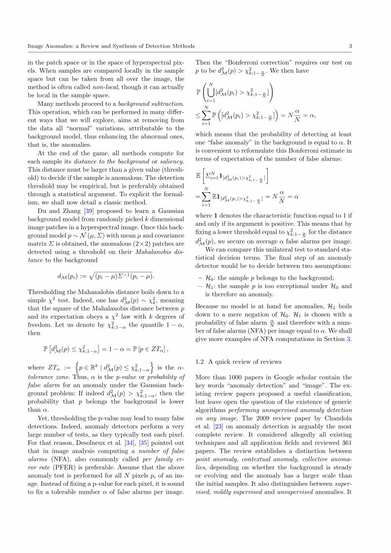
Image Anomalies: a Review and Synthesis of Detection Methods 3

in the patch space or in the space of hyperspectral pix-

els. When samples are compared locally in the sample

space but can be taken from all over the image, the

method is often called non-local, though it can actually

be local in the sample space.

Many methods proceed to a background subtraction.

This operation, which can be performed in many differ-

ent ways that we will explore, aims at removing from

the data all “normal” variations, attributable to the

background model, thus enhancing the abnormal ones,

that is, the anomalies.

At the end of the game, all methods compute for

each sample its distance to the background or saliency.

This distance must be larger than a given value (thresh-

old) to decide if the sample is anomalous. The detection

threshold may be empirical, but is preferably obtained

through a statistical argument. To explicit the formal-

ism, we shall now detail a classic method.

Du and Zhang [39] proposed to learn a Gaussian

background model from randomly picked k dimensional

image patches in a hyperspectral image. Once this back-

ground model p ∼ N (µ,Σ) with mean µ and covariance

matrix Σ is obtained, the anomalous (2×2) patches are

detected using a threshold on their Mahalanobis dis-

tance to the background

dM(pi) :=√

(pi − µ)Σ−1(pi − µ).

Thresholding the Mahanalobis distance boils down to a

simple χ2 test. Indeed, one has d2M(p) ∼ χ2k, meaning

that the square of the Mahalanobis distance between p

and its expectation obeys a χ2 law with k degrees of

freedom. Let us denote by χ2k;1−α the quantile 1 − α,

then

P[d2M(p) ≤ χ2

k;1−α]

= 1− α = P [p ∈ ZTα] ,

where ZTα :={p ∈ Rk | d2M(p) ≤ χ2

k;1−α

}is the α-

tolerance zone. Thus, α is the p-value or probability of

false alarm for an anomaly under the Gaussian back-

ground problem: If indeed d2M(p) > χ2k;1−α, then the

probability that p belongs the background is lower

than α.

Yet, thresholding the p-value may lead to many false

detections. Indeed, anomaly detectors perform a very

large number of tests, as they typically test each pixel.

For that reason, Desolneux et al. [34], [35] pointed out

that in image analysis computing a number of false

alarms (NFA), also commonly called per family er-

ror rate (PFER) is preferable. Assume that the above

anomaly test is performed for all N pixels pi of an im-

age. Instead of fixing a p-value for each pixel, it is sound

to fix a tolerable number α of false alarms per image.

Then the “Bonferroni correction” requires our test on

p to be d2M(p) > χ2k;1− α

N. We then have

P

(N⋃i=1

[d2M(pi) > χ2k;1− α

N]

)

≤N∑i=1

P(

[d2M(pi) > χ2k;1− α

N])

= Nα

N= α,

which means that the probability of detecting at least

one “false anomaly” in the background is equal to α. It

is convenient to reformulate this Bonferroni estimate in

terms of expectation of the number of false alarms:

E[ΣNi=11[d2M(pi)>χ2

k;1− αN

]

]=

N∑i=1

E1[d2M(pi)>χ2k;1− α

N] = N

α

N= α

where 1 denotes the characteristic function equal to 1 if

and only if its argument is positive. This means that by

fixing a lower threshold equal to χ2k;1− α

Nfor the distance

d2M(p), we secure on average α false alarms per image.

We can compare this unilateral test to standard sta-

tistical decision terms. The final step of an anomaly

detector would be to decide between two assumptions:

– H0: the sample p belongs to the background;

– H1: the sample p is too exceptional under H0 and

is therefore an anomaly.

Because no model is at hand for anomalies, H1 boils

down to a mere negation of H0. H1 is chosen with a

probability of false alarm αN and therefore with a num-

ber of false alarms (NFA) per image equal to α. We shall

give more examples of NFA computations in Section 3.

1.2 A quick review of reviews

More than 1000 papers in Google scholar contain the

key words “anomaly detection” and “image”. The ex-

isting review papers proposed a useful classification,

but leave open the question of the existence of generic

algorithms performing unsupervised anomaly detection

on any image. The 2009 review paper by Chandola

et al. [23] on anomaly detection is arguably the most

complete review. It considered allegedly all existing

techniques and all application fields and reviewed 361

papers. The review establishes a distinction between

point anomaly, contextual anomaly, collective anoma-

lies, depending on whether the background is steady

or evolving and the anomaly has a larger scale than

the initial samples. It also distinguishes between super-

vised, mildly supervised and unsupervised anomalies. It


Fig. 1 Examples of industrial images with anomalies to detect. From left to right a suspicious mammogram [56], an underseamine [96], a defective textile pattern [139] and a defective wheel [136].

revises the main objects where anomalies are sought

for (images, text, material, machines, networks, health,

trading, banking operations, etc.) and lists the preferred

techniques in each domain. Then it finally proposes the

following classification of all involved techniques.

1. Classification based anomaly detection, e.g.,

SVM, Neural networks. These techniques train a

classifier to distinguish between normal and anoma-

lous data in the given feature space. Classification is

either multi-class (normal versus abnormal) or one-

class (only trains to detect normality, that is, learns

a discriminative boundary around normal data).

Among the one-class detection methods we have the

Replicator Neural Networks (auto-encoders).

2. Nearest neighbor based anomaly detection.

The basic assumption of these methods is that nor-

mal data instances occur in dense neighborhoods,

while anomalies occur far from their closest neigh-

bors. This can be measured by the distance to the

kth nearest neighbor or as relative density.

3. Clustering based anomaly detection. Normal

data instances are assumed to belong to a cluster

in the data, while anomalies are defined as those

standing far from the centroid of their closest clus-

ter.

4. Statistical anomaly detection. Anomalies are

defined as observations unlikely to be generated by

the “background” stochastic model. Thus, anoma-

lies occur in the low probability regions of the back-

ground model. Here the background models can

be: parametric (Gaussian, Gaussian mixture, regres-

sion), or non-parametric and built, e.g., by a kernel

method.

5. Spectral anomaly detection. The main tool here

is principal component analysis (PCA) and its gen-

eralizations. Its principle is that an anomaly has de-

viant coordinates with respect to normal PCA co-

ordinates.

6. Information theoretic anomaly detection.

These techniques analyze the information content

of a data set using information theoretic measures,

such as, the Kolomogorov complexity, the entropy,

the relative entropy, among others.

This excellent review is perhaps nevertheless biting off

more than it could possibly chew. Indeed, digital ma-

terials like sound, text, networks, banking operations,

etc. are so different that it was impossible to exam-

ine in depth the role of their specific structures for

anomaly detection. By focusing on images, we shall

have a much focused discussion involving their specific

structure yielding natural vector samples (color or hy-

perspectral, pixels, patches) and specific structures for

these samples, such as self-similarity and sparsity.

The above review by Chandola et al. [23] is fairly

well completed by the more recent review by Pimentel

et al. [114]. This paper presents a complete survey of

novelty detection methods and introduces a classifica-

tion into five groups.

1. Probabilistic novelty detection. These meth-

ods are based on estimating a generative proba-

bilistic model of the data (either parametric or non-

parametric).

2. Distance-based methods. These methods rely

on a distance metric to define similarity among

data points (clustering, nearest-neighbour and self-

similar methods are included here).

3. Reconstruction-based methods. These methods

seek to model the normal component of the data

(background), and the reconstruction error or resid-

ual is used to produce an anomaly score.

4. Domain-based methods. They determine the lo-

cation of the normal data boundary using only the

data that lie closest to it, and do not make any as-

sumption about data distribution.

5. Information-theoretic methods. These methods

require a measure (information content) that is sen-

sitive enough to detect the effects of anomalous

points in the dataset. Anomalous samples, for exam-

ple, are detected by a local Gaussian model, which

starts this list.

Our third reviewed review was devoted to anomaly

detection in hyperspectral imagery [93]. It completes


three previous comparative studies, namely [129],

[65] and [92]. Matteoli et al. [93] conclude that

most of the techniques try to cope with background

non-homogeneity, and attempt to remove it by de-

emphasizing the main structures in the image, which

we can interpret as background subtraction.

For the same authors, an anomaly can be defined as

an observation that deviates in some way from the back-

ground clutter. The background itself can be identified

from a local neighborhood surrounding the observed

pixel, or from a larger portion of the image. They also

suggest that the anomalies must be sparse and small

to make sense as anomalies. Also, no a-priori knowl-

edge about the target’s spectral signature should be

required. The question in hyperspectral imagery there-

fore is to “find those pixels whose spectrum significantly

differs from the background”. We can summarize the

findings of this review by examining the five detection

techniques that are singled out:

1. Modeling the background as a locally Gaus-

sian model [117] and detecting anomalous pixels

by their Mahanalobis distance to the local Gaus-

sian model learned from its surrounding at some dis-

tance. This famous method is called the RX (Reed-

Xiaoli) algorithm.

2. Gaussian-Mixture Model based Anomaly De-

tectors [5, 18, 59, 129]. The optimization is done by

stochastic expectation minimization [91]. The detec-

tion methodology is similar to the locally Gaussian

model, but the main difference is that background

modeling becomes global instead of local.

The technical difficulty raised by this more complex

model is the variety of clustering algorithms that

can be used [41, 42], and the thorny question of find-

ing the adequate number of clusters as addressed in

[43] and [111].

3. The Orthogonal Subspace Projection ap-

proach. It performs a background estimation via

a projection of pixel samples on their main compo-

nents after an SVD has been applied to all samples.

Subtracting the resulting image amounts to a back-

ground subtraction and therefore delivers an image

where noise and the anomalies dominate.

4. The kernel RX algorithm [73] which proceeds

by defining a (Gaussian) kernel distance between

pixel samples and considering that it represents a

Euclidean distance in a higher dimension feature

space. (This technique is also proposed in [94] for oil

slick detection.) A local variant of this method [116]

performs an OSP suppression of the background,

defined as one of the four subspaces spanned by

the pixels within four neighboring subwindows sur-

rounding the pixel at some distance.

5. Background support region estimation by

Support Vector Machine [6]. Here the idea is

that it is not necessary to model the background,

but that the main question is to model its support

and to define anomalies as observations away from

this support.

Our last reviewed review, by Olson et al. [106],

compares “manifold learning techniques for unsuper-

vised anomaly detection” on simulated and real images.

Manifold methods assume that the background samples

span a manifold rather than a linear space. Hence PCA

might be suboptimal and must be replaced by a non-

linear change of coordinates. The authors of the review

consider and three kinds for this change of coordinates:

1. Kernel PCA, introduced by Scholkopf et al. [122]

and adapted to the anomaly detection problem by

Hoffmann [62].

2. The Parzen density estimator, which is actually

interpreted as the simplest instance of kernel PCA

[62, 108].

3. The diffusion map [29, 74], which in this frame-

work appears as a variant of kernel PCA.

We shall review these techniques in more detail in Sec-

tion 2. In these methods, the sample manifold M is

structured by a Gaussian “distance”

k(xj , xj) = e−1h2||xi−xj ||2 .

The methods roughly represent the samples by coor-

dinates computed from the eigenvectors and eigenval-

ues of the matrix K = (k(xi, xj))ij . This amounts in

all cases to a nonlinear change of coordinates. Then,

anomalous samples are detected as falling apart from

the manifold. The key parameter h is chosen in the

examples so that the isolevel surface of the distance

function wraps tightly the inliers.

The review compares the ROC curves of the differ-

ent methods (PCA, kernel PCA, Parzen, diffusion map)

and concludes that small ships on a sea landscape are

better detected by kernel PCA. Since the review only

compares ROC curves between the different methods,

it avoids addressing the detection threshold issue.

Discussion. The above four highly cited reviews made

an excellent job of considering countless papers and

proposing a categorization of methods. Nevertheless,

their final map of the methods is an exhaustive in-

ventory where methods are distributed according to

what they do, rather than to what they assume on

background and anomaly. Nevertheless, the Pimentel

et al. [114] review is actually close to classify methods

by structural assumptions on the background, and we


shall follow this lead. The above reviews do not con-

clude on a unified statistical decision framework. Thus,

while reusing most of their categories, we shall attempt

at reorganizing the panorama according to three main

questions:

– What is the structural assumption made on the

background: in other terms what is “normal”?

– How is the decision measurement computed?

– How is the anomaly detection threshold defined and

computed, and what guarantees are met?

Our ideal goal would be to find out the weakest

(and therefore most general) structural assumption on

normal data, and to apply to it the most rigorous sta-

tistical test. In other words, the weaker the assump-

tions of normality, the more generic the detector will

be. Before proceeding to a classification of anomaly de-

tection methods, we shall examine several related ques-

tions which share some of their tools with anomaly de-

tection.

1.3 What anomaly detection isn’t

1.3.1 Not a classification problem

Most papers and reviews on anomaly detection agree

that multi-class classification techniques like SVM can

be discarded, because anomalies are generally not ob-

served in sufficient number and lack statistical coher-

ence. There are exceptions like the recent method in-

troduced by Ding et al. [37]. This paper assumes the

disposition of enough anomalous samples to learn clas-

sification parameters from the data themselves. Given

several datasets with dimensions from 8 to 50 with mod-

erate size (a few hundreds to a few thousand samples),

this paper applies classic density estimators to sizable

extracts of the normal set (k-means, SVM, Gaussian

mixture), then learns the optimal thresholds for each

classifier and finally compares the performance of these

classifiers.

While in many surface defect detection problems,

the defect can be of any shape or color, in some in-

dustrial applications known recurrent anomalies are

the target of defect detectors. In this case a train-

ing database can be produced and the detection algo-

rithm is tuned for the detection of the known defects

[69, 146, 148]. For example, Soukup and Huber-Mork

[128] proposed to detect rail defects in a completely su-

pervised manner by training a classical convolutional

neural networks on a dataset of photometric stereo im-

ages of metal surface defects. Another neural-network

based method was proposed by Kumar [72]. This paper

on the detection of local fabric defects, first performs

a PCA dimension reduction on 7× 7 windows followed

by the training of a neural network on a base of detects

/ non-detects, thus again performing two-class classifi-

cation.

To detect changes on optical or SAR satellite im-

ages, many methods compare a pair of temporally close

images, or more precisely the subtraction between them

in the case of optical images [13, 15, 81, 82, 134, 150,

151], or the log-ratio for SAR images [12, 22, 70, 79].

However these methods often work on a pair of images

where a change is known to have occurred (such as a

forest fire [15, 22], an earthquake [46, 144] or a flood

[27, 79]), and thus have an a priori for a two class dis-

tribution, which leads to classification techniques.

Conclusions.

1.3.2 More than a saliency measure

A broad related literature exists on saliency measures.

They associate to each image a saliency map, which is

a scalar positive function that can be visualized as an

image where the brighter the pixel, the more salient it

is. The goal of automatic saliency measures is to em-

ulate the human perception. Hence saliency measures

are often learned from a large set of examples associat-

ing with images their average fixation maps by humans.

For example, Tavakoli et al. [131] designed an anomaly

detector trained on average human fixation maps learn-

ing both the salient parts and their surround vectors as

Gaussian vectors. This reduced the problem to a two

class Bayesian classification problem.

The main difference with anomaly detectors is that

many saliency measures try to mimic the human vi-

sual perception and therefore are allowed to introduce

semantic prior knowledge related to the perceptual sys-

tem (e.g., face detectors). This approach works particu-

larly well with deep neural networks because attention

maps obtained by gaze trackers can be used as a ground

truth for the training step. SALICON by Huang et al.

[64] is one of these deep neural networks architecture

achieving state of the art performance.

Saliency measures deliver saliency maps, in contrast

to anomaly detectors that are requested to give a binary

map of the anomalous regions. We can exclude from our

review supervised saliency methods based on learning

from humans. Yet we cannot exclude the unsupervised

methods that are based, like anomaly detectors, on a

structural model of the background. The only differ-

ence of such saliency maps with anomaly detectors is

that that anomaly detectors would require to add a last

thresholding step after the saliency map is computed,

to transform it into a binary detection map.


Interesting methods for example assign a saliency

score to each tested pixel feature based on the inverse

of the histogram bin value to which it belongs. In [118]

a saliency map is obtained by combining 32 multiscale

oriented features obtained by filtering the image with

oriented Gabor kernels. A weighted combination of the

most contrasted channels for each orientation yields a

unique multiscale orientation channel co(i) for each ori-

entation. Then the histograms ho of these channels coare computed and each pixel i with value co(i) is given

a weight which is roughly inversely proportional to its

value ho(co(i)) in the histogram. The same rarity mea-

surement is applied to the colors after PCA. Summing

all of these saliency maps one obtains something simi-

lar to what is observed with gaze trackers: the salient

regions are the most visited.

Similarly, image patches are represented by Borji

and Itti [11] using their coefficients on a patch dictio-

nary learned on natural images. Local and global image

patch rarities are considered as two “complementary

processes”. Each patch is first represented by a vector

of coefficients that linearly reconstruct it from a learned

dictionary of patches from natural scenes (“normal”

data). Two saliency measures (one local and one global)

are calculated and fused to indicate the saliency of each

patch. The local saliency is computed as the distinctive-

ness of a patch from its surrounding patches, while the

global saliency is the inverse of a patch’s probability

of happening over the entire image. The final saliency

map is built by normalizing and fusing local and global

saliency maps of all channels from both color systems.

(Patch rarity is measured both in RGB and Lab color

spaces.)

One can consider the work by Murray et al. [101],

as a faithful representative of the multiscale center-

surround saliency methods. Its main idea is to:

• apply a multi-scale multi-orientation wavelet pyra-

mid to the image;

• measure the local wavelet energy for each wavelet

channel at each scale and orientation;

• compute a center-surround ratio for this energy;

• obtain in that way wavelet contrast coefficients that

have the same spatial multi-scale sampling as the

wavelet pyramid itself;

• apply the reverse wavelet pyramid to the contrast

coefficients to obtain a saliency map.

This is a typical saliency-only model, for which an ad-

equate detection threshold is again missing.

Conclusions. Saliency detection methods learned from

human gaze tracking are semantic methods that fall

off our inquiry. But unsupervised saliency measures de-

liver a map that only needs to be adequately thresh-

olded to get an anomaly map. They therefore pro-

pose mechanisms and background structure assump-

tions that are relevant for anomaly detection. Con-

versely, most anomaly detectors also deliver a saliency

map before thresholding. The last three generic saliency

measures listed are tantalizing. Indeed, they seem to do

a very good job of enhancing anomalies by measuring

rarity. Notwithstanding, they come with no clear mech-

anism to transform the saliency map into a probabilistic

one that might allow hypothesis testing and eventually

statistically motivated detection thresholds.

1.3.3 A sketch of our proposed classification

The anomaly detection problem has been generally han-

dled as a “one-class” classification problem. The 2003

very complete review by Markou and Singh [90] con-

cluded that most research on anomaly detection was

driven by modeling background data distributions, to

estimate the probability that test data do not belong to

such distributions. Hence the mainstream methods can

be classified by their approach to background modeling.

Every detection method has to do three things:

(a) to model the anomaly-free “background”. This

background model may be constructed from sam-

ples of various sizes extracted from the given image

(or an image database): pixels (e.g. in hyperspectral

images), patches, local features (e.g. wavelet coeffi-

cients).

(b) to define a measure on the observed data evaluat-

ing how far its samples are from their background

model. Generally, this measure is a probability of

false alarm (or even better, as we shall see, an ex-

pectation of the number of false alarms) associated

with each sample.

(c) to define the adequate (empirically or statistically

motivated) threshold value on the measure obtained

in b).

The structure chosen for the background model appears

to us as the most important difference between meth-

ods. Hence we shall primarily classify the methods by

the assumed structure of their background model, and

the way a distance of samples to the background model

is computed. Section 3 will then be devoted to the com-

putation of the detection thresholds.

We shall examine in detail five generic structures for

the background:

1. the background can be modeled by a probability

density function (pdf), which is either parametric,

such as, a Gaussian, or a Gaussian mixture, or is

obtained by interpolation from samples by a kernel


density estimation method; this structure leads to

detect anomalies by hypothesis testing on the pdf;

2. the background is globally homogeneous (allowing

for a fixed reference image, a global Fourier or a con-

volutional neural network model generally followed

by background subtraction);

3. the background is locally spatially homogeneous

(leading to center-surround methods);

4. the background is sparse on a given dictionary or

base (leading to variational decomposition models).

5. the background is self-similar (in the non-local

sense that for each sample there are other similar

samples in the image).

2 Detailed analysis of the main anomaly

detection families

The main anomaly detection families can be analyzed

from their structural assumptions on the background

model. In what follows we present and discuss the five

different families that we announced.

2.1 Stochastic background models

The principle of these anomaly detection methods is

that anomalies occur in the low probability regions of

the background model. The stochastic model can be

parametric (Gaussian, Gaussian mixture, regression),

or non-parametric. For example in “spectral anomaly

detection” as presented by Chandola et al. [23], an

anomaly is defined by having deviant coordinates with

respect to normal PCA coordinates. This actually as-

sumes a Gaussian model for the background.

Gaussian background model. The Gaussian background

assumption may expand to image patches. Du and

Zhang [39] proposed to build a Gaussian background

model from random 2 × 2 image patches in a hyper-

spectral image. Once this background model (µ,Σ) is

obtained, the anomalous (2 × 2) patches are detected

using a threshold on their Mahalanobis distance to the

background Gaussian model. The selection of the image

blocks permitting to estimate the Gaussian patch model

(µ,Σ) is performed by a RANSAC procedure [47], pick-

ing random patches in the image and excluding progres-

sively the anomalous ones.

Goldman and Cohen [54], aiming at sea-mine detec-

tion, propose a detection scheme that does not rely on

a statistical model of the targets. It performs a back-

ground estimation in a local feature space of principal

components (this again amounts to building a Gaussian

model). Then, hypothesis testing is used for the detec-

tion of anomalous pixels, namely those with an exceed-

ingly high Mahalanobis distance to the Gaussian distri-

bution (Section 1.1). This detects potentially anoma-

lous pixels, which are thereafter grouped and filtered

by morphological operators. This ulterior filter suggests

that the first stage may yield many false alarms.

Pdf estimation. Sonar images have a somewhat spe-

cific anisotropic structure that leads to model the back-

ground using signal processing methods. For exam-

ple, in [100] the authors proposed to adapt an ARCH

model, thus obtaining a statistical detection model for

anomalies not explained by the non-causal model. This

method is similar to the detection of scratches in musi-

cal records [107].

Cohen et al. [28] detect fabric defects using a Gaus-

sian Markov Random Fields model. The method com-

putes the likelihood of patches of size 32×32 or 64×64

according to the model learned on a database free of

defects. The patches are then classified as anomalous

or defect-free thanks to a likelihood ratio test.

Tarassenko et al. [130] identify abnormal masses

in mammograms by assuming that abnormalities are

uniformly distributed outside the boundaries of nor-

mality (defined using an estimation of the probabil-

ity density function from training data). If a feature

vector falls in a low probability region (using a pre-

determined threshold), then this feature vector is con-

sidered to be novel. The process to build the back-

ground model is complex and involves selecting five lo-

cal features, equalizing their means and variances to

give them the same importance, clustering the data setinto four classes, and estimating for each cluster its pdf

by a non-parametric method (i.e., Parzen window inter-

polation). Finally, a feature vector is considered anoma-

lous if it has low probability for each estimated pdf.

Such a non-parametric pdf estimate has of course an

over-fitting or under-fitting risk, due to the fact that

training data are limited.

Gaussian Mixture. The idea introduced by Xie and

Mirmehdi [147] is to learn a texture model based on

Julezs’ texton theory [71]. The textons are interpreted

as image patches following a Gaussian model. Thus a

random image patch is assumed to follow a Gaussian

mixture model (GMM), which is therefore estimated

from exemplar images by the expectation-maximization

algorithm (EM). The method works at several scales in

a Gaussian pyramid with fixed size patches (actually

5 × 5). The threshold values for detecting anomalies

are learned on a few images without defects in the fol-

lowing way: At each scale, the minimum probability in


the GMM over all patches is computed. These proba-

bilities serve as detection thresholds. A patch is then

considered anomalous if its probability is lower than

the minimum learned on the faultless textures on two

consecutive dyadic scales in the Gaussian pyramid. A

saliency map is obtained by summing up these consec-

utive probability excesses. Clearly, this model can be

transformed from a saliency map to an anomaly de-

tector by using hypothesis testing on the background

Gaussian mixture model. Gaussian mixture modeling

has been long classical in hyperspectral imagery [5] to

detect anomalies. In that case, patches are not needed

as each hyperspectral pixel already contains rich mul-

tidimensional information.

Gaussian Stationary process. Grosjean and Moisan

[56] propose a method that models the background im-

age as a Gaussian stationary process, which can also

be modeled as the result of the convolution of a white

Gaussian noise model with an arbitrary kernel, in other

terms a colored noise. This background model is rather

restrictive, but it is precise and simple to estimate. The

Gaussian model is first estimated. Then the image is fil-

tered either with low-pass filters (to detect global peaks

in the texture) or center-surround filters (to detect lo-

cally contrasted peaks in the texture). The Gaussian

probability density function of each of these filtered im-

ages is easily computed. Finally, a probabilistic detec-

tion threshold for the filtered images is determined by

bounding the NFA as sketched in Section 1.1 (we shall

give more details on this computation in Section 3.1.)

Conclusions. To summarize, in the above methods re-

lying on probabilistic background models, outliers are

detected as incoherent with respect to a probability

distribution estimated from the input image(s). The

anomaly detection threshold is a statistical likelihood

test on the learned background model. In all cases, it

gives (or could give) a p-value for each detection. So,

by tightening the detection thresholds, one can easily

control the number of false alarms, as done by Grosjean

and Moisan [56] (see Section 1.1).

2.2 Homogeneous background model

These methods estimate and (generally) subtract the

background from the image to get a residual image rep-

resentation on which detection is eventually performed.

We shall examine different ways to do so: by using

Fourier modeling, auto-encoder networks, or by sub-

traction of a smooth or fixed background.

Fourier background model. Perhaps the most successful

background based method is the detection of anomalies

in periodic patterns of textile [113, 139, 140]. This can

be done naturally by cutting specific frequencies in the

Fourier domain and thresholding the residual to find

the defects. For example Tsai and Hsieh [139] remove

the background by a frequency cutoff. Then a detec-

tion threshold using a combination of the mean and

the variance of the residual yields a detection map.

Similarly, Tsai and Huang [140] propose an auto-

matic inspection of defects in randomly textured sur-

faces which arise in sandpaper, castings, leather, and

other industrial materials. The proposed method does

not rely on local texture features, but on a background

subtraction scheme in Fourier domain. It assumes that

the spread of frequency components in the power spec-

trum space is isotropic, and with a shape that is close to

a circle. By finding an adequate radius in the spectrum

space, and setting to zero the frequency components

outside the selected circle, the periodic, repetitive pat-

terns of statistical textures are removed. In the restored

image, the homogeneous regions in the original image

get approximately flat, but the defective region is pre-

served. According to the authors, this leads to convert

the defect detection in textures into a simple threshold-

ing problem in non-textured images. This thresholding

is done using a statistical process control (SPC) bina-

rization method,

fb(x, y) =

{255 if µ− kσ 6 f(x, y) 6 µ+ kσ

0 otherwise,

where k is a control parameter, µ is the residual image

average and σ2 its variance. Regions set to zero are then

detected.

Perng et al. [113] focus on anomaly detection dur-

ing the production of bolts and nuts. The method starts

by creating normalized unwrapped images of the pat-

tern on which the detection is performed. The first step

consists in removing the “background” by setting to

zero some Fourier coefficients. Indeed, the background

pattern being extremely periodic, is almost entirely re-

moved by canceling large Fourier coefficients. The mean

µ and the variance σ2 of the residual are then com-

puted. This residual is then thresholded using the SPC

binarization method of Tsai and Huang [140].

Aiger and Talbot [3] propose to learn a Gaussian

background Fourier model of the image Fourier phase

directly from the input image. The method assumes

that only a few sparse defaults are present in the pro-

vided image. First a “phase only transform (PHOT)”

is applied to the image. The Fourier transform of an

image contains all the information of its source inside

the modulus of the Fourier coefficients and their phase.


The phase is known to contain key positional elements

of the image, while the modulus relates more to the

image texture, and therefore to its background. To il-

lustrate this fact, RPNs are well known models for a

wide class of “microtextures” as explained in Galerne

et al. [50]. A RPN is a random image where the Fourier

coefficients have deterministic moduli (identical to the

reference texture), but random, uniform, independent

phases. Another illustration of the role of phase and

modulus is obtained noticing that a Gaussian noise has

uniform random phase. The PHOT amounts to invert

the Fourier transform of an image after normalizing

the Fourier coefficients modulus, thus keeping only the

structural information contained in the phase. A local

anomaly is expected to have a value in excess compared

to the PHOT. Anomalous pixels are therefore detected

as peaks of the Mahalanobis distance of their values

to the background modelled as Gaussian distributed.

Hence, a probability of false alarm can be directly com-

puted in this ideal case. The detection method can be

also applied after convolving the PHOT transformed

image with a Gaussian, to detect blobs instead of sin-

gle pixels.

Xie and Guan [145] introduced a method to detect

defects in periodic wafer images. By estimating the pe-

riods of the repeating pattern, the method obtains a

“golden template” of the patterned wafer image under

inspection. No other prior knowledge is required. The

estimated defect-free background pattern image is then

subtracted to find out possible defects.

Neural-network-based background model. The general

idea is to learn the background model by using a neuralnetwork trained on normal data. Under the assumption

that the background is homogeneous, the “replicator”

neural networks proposed by Hawkins et al. [58] can be

used to learn this model. These networks were intro-

duced in section 1.2.

Perhaps the most important application of anomaly

detection in industry is surface defect detection. Iivari-

nen [66] proposes an efficient technique to detect de-

fects in surface patterns. A statistical self-organizing

map (SOM) is trained on defect-free data, using hand-

picked features from co-occurrence matrices and tex-

ture unit elements. The SOM is then able to separate

the anomalies, which are supposed to have a different

feature distribution. As can be seen in Xie [146] which

reviews surface defect detection techniques, many sur-

face defect detection methods work similarly. Texture

features are selected, and defects are detected as being

not well explained by the feature model.

Similarly Chang et al. [24] presented an unsuper-

vised clustering-based automatic wafer inspection sys-

tem using self-organizing neural networks. An [4] pro-

posed to train a variational autoencoder (VAE), and to

compute from it an average reconstruction probability,

which is a different measure than just looking at the

difference between the input and output. Given a new

data point, a number of samples are drawn from the

trained probabilistic encoder. For each code sample, the

probabilistic decoder outputs the corresponding mean

and variance parameters. Then, the probability of the

original data being generated from a Gaussian distribu-

tion having these parameters is calculated. The average

probability, named reconstruction probability, among

all drawn samples is used as an anomaly score.

Mishne et al. [97] presented an encoder-decoder

deep learning framework for manifold learning. The

encoder is constrained to preserve the locality of the

points, which improves the approximation power of

the embedding. Outliers are detected based on the au-

toencoder reconstruction error. The work of Schlegl

et al. [121] is in the same direction as using an au-

toencoder and looking at the norm between the origi-

nal and the output. A Generative Adversarial Network

(GAN) [55] is trained (generator + discriminator) by

using anomalous-free data. Then, given a new test im-

age a representation in latent space is computed (by

backpropagation), and the GAN reconstruction is com-

pared to the input. The discriminator cost is then used

alongside the representation of the input by the network

to find the anomalies. There is, however, no guarantee

that the latent representation found would do good for

anomaly free examples. Hence, it is not clear why the

discriminator cost would detect anomalies.

Smooth or fixed background model. Many surface defect

detectors fall into that category. For example, a com-

mon procedure to detect defects in semiconductors is

to use a fixed reference clean image and apply some

detection procedure to the difference of the observed

image and the reference pattern [38, 60, 126, 141, 142].

Since for different chips, the probability of defects ex-

isting at the same position is very low, one can extract

a standard reference image by combining at least three

images (by replacing pixels located in defects by the

pixels located in the corresponding location of another

image)[80]. Similar ideas have been exploited for the

detection of defects in patterned fabrics [104]. In [105],

nonconforming regions are detected by subtracting a

golden reference image and processed in the Wavelet

domain.

A very recent and exemplary method to detect

anomalies in smooth materials is the one proposed

by Tout et al. [137]. In this paper, the authors develop

a method for the fully automatic detection of anomalies


on wheels surface. First, the wheel image are registered

to a fixed position. For each wheel patch in a given po-

sition, a linear deterministic background model is de-

signed. Its basis is made of a few low degree polyno-

mials combined with a small number of basis functions

learned as the first basis vectors of a PCA applied to

exemplar data. The acquisition noise is accurately mod-

eled by a two-parameter Poisson noise. The parameters

are easily estimated from the data. The background es-

timation is a mere projection of each observed patch

on the background subspace. The residual, computed

as the difference between the input and the projection,

can contain only noise-and anomalies. Thus, classic hy-

pothesis testing on the norm of the residual of each

patch will yield an automatic detection threshold. This

method is clearly adapted to defect detection on smooth

surfaces.

Conclusions. Homogeneous background model based

anomaly detection methods are compelling detectors

used in a wide variety of applications. They avoid

proposing a stochastic model for an often complex back-

ground by computing the distance to the background

or doing background subtraction. However this simpli-

fication comes at a cost: some algorithms are hard to

generalize to new applications, and the detection deci-

sion mechanism is generally not statistically justified,

with the exception of some methods, like Tout et al.

[137].

2.3 Local homogeneity models: center-surround

detection.

These methods are often used for creating saliency

maps. Their rationale is that anomalies (or saliency)

occur as local events contrasting with their surround-

ings.

In one of the early papers on this topic, Itti et al.

[68] propose to compute a set of center-surround lin-

ear filters based on color, orientation and intensity. The

filters are chosen to only have positive output values.

The resultant maps are normalized by stretching their

response so that the max is at a pre-specified value.

These positive feature maps are then summed up to

produce a final saliency map. Detection is then done on

a simple winner-takes-all scheme on the maximum of

the response maps. This method is applied in Itti and

Koch [67] to detect vehicles via their saliency in huge

natural or urban images. It has also been generalized

to video in Mahadevan et al. [85].

The method was expanded by Gao et al. [51]. The

features in this paper are basically the same as those

proposed by Itti and Koch [67], that is, color features,

intensity features, and a few orientation filters (Gabor

functions, wavelets). This last paper does detection on

image and video with center-surround saliency detector.

It directly compares its results to those of Itti and Koch

[67] and takes similar features, but works differently

with them. In particular it computes center-surround

discrimination scores for the features, and puts in doubt

the linearity of center-surround filters and the need for

computing a (necessarily nonlinear) probability of false

alarm in the background model. In fact, they claim [51]:

“In particular, it is hypothesized that, in the ab-

sence of high-level goals, the most salient loca-

tions of the visual field are those that enable

the discrimination between center and surround

with smallest expected probability of error.”

The difficulty of center-surround anomaly detection

is faced by Honda and Nayar [63], who introduced a

generic method which tentatively works on all types

of images. The main idea is to estimate a probability

density for sub-regions in an image, conditioned upon

the areas surrounding these sub-regions. The estima-

tion method employs independent component analysis

and the Karhunen-Loeve transform (KLT) to reduce di-

mensionality and find a compact representation of the

region space and its surroundings, with elements as in-

dependent as possible. Anomaly is again defined as a

subregion with low conditional probability with respect

to its surrounding. This is both a coarse grained and

complex method.

Scholkopf et al. [123] and Tax and Duin [133] ex-

tended SVM to the problem of one-class detection (sup-

port estimation). The general idea is that by assuming

that only a small fraction of the training data consist

of anomalies, we can optimize the decision function of a

classifier to predict if a point belongs or not to the nor-

mal class. The goal is to find the simplest or smallest

region that is compatible to observing a given fraction

of anomalies in the training set. In [57], the authors

presented an ensemble-learning anomaly detection ap-

proach by optimizing an ensemble of kernel-based one-

class classifiers.

Very recently, Ruff et al. [120] introduced a novel

approach to detect anomalies using deep-learning that

is inspired in the same ideas. The method, named Deep

Support Vector Data Description (Deep SVDD), trains

a deep neural network by minimizing the volume of a

hypersphere that encloses the network representations

of the data.

In the famous Reed-Xiaoli (RX) algorithm [117] the

pixels of a hyperspectral optical image are assumed to

follow a Gaussian non-stationary multivariate random

process with a rapidly fluctuating space-varying mean


vector and a more slowly space-varying covariance ma-

trix. This “local normal model” for the background

pixels is learned from an outer window from which a

guard window has been subtracted, as it might contain

the anomaly. Then detection is performed by threshold-

ing the Mahanalobis distance of the pixel of interest to

the local Gaussian model, as described in Section 1.1.

It may be noticed that a previous rough background

subtraction is performed by a local demeaning using a

sliding window [25, 88]. Matteoli et al. [93] points out

two main limitations of the RX method: first, the dif-

ficulty of estimating locally a high dimensional covari-

ance matrix, and second the fact that a local anomaly

is not necessarily a global anomaly: an isolated tree in

a meadow would be viewed as an anomaly, even if its

stands close to a wood of the same trees. Nevertheless,

RX remains a leading algorithm and it has even online

versions: See, e.g., [48] for the successful application of

RX after a dimensional reduction by random projec-

tions, inspired from compressed sensing.

Conclusions. Most presented center-surround anomaly

detectors produce a saliency map, but as previously

mentioned in Section 1.3.2, while saliency detectors are

tantalizing since they propose simple and efficient rar-

ity measurements, they provide no detection mecha-

nism (threshold value). Several above reviewed center-

surround methods attempt to remedy that. But then,

the method becomes quite heavy as it requires esti-

mating a local stochastic model for both the center and

surround. Hence we are forced back to two-class clas-

sification with fewer samples and a far more complex

methodology.

2.4 Sparsity-based background models and its

variational implementations

One recent non-parametric trend is to learn a sparse

dictionary representing the background (i.e., normal-

ity) and to characterize outliers by their non-sparsity.

Margolin et al. [89] propose a method for building

salient maps by a conjunction of pattern distinctness

and color distinctness. They claim that for pattern dis-

tinctness, patch sparsity is enough to characterize vi-

sual saliency. They proceed by:

(a) Computing the PCA of all patches (of fixed size –

typically 8× 8) in the image;

(b) Computing the pattern saliency of a patch p as

P (p) := ‖p‖1 where the l1 norm is computed on

the PCA coordinates.

(c) The pattern saliency measure is combined (by mul-

tiplication) with a color distinctness measure, that

measures the distance of each color super pixel to

its closest color cluster. The final map therefore is

D(p) := P (p)C(p) where C(p) is the color distinct-

ness.

(d) The final result is a product of this saliency map

with (roughly) a Gaussian centered in the center of

mass of the previous saliency map.

We now look at sparsity models that learn the

background model as a dictionary on which “normal”

patches would have to be represented by a sparse lin-

ear combination of the elements of the dictionary (and

anomalous patches tentatively would not). Sparse dic-

tionary learning, popularized by the K-SVD algorithm

[2] and [119] and online learning methods [86], has been

successful for many signal representation applications

and in particular for image representation and denois-

ing [87].

Cong et al. [31], Zhao et al. [152] proposed a com-

pletely unsupervised sparse coding approach for detect-

ing abnormal events in videos based on online sparse

reconstructibility of query signals using a learned event

dictionary. These methods are based on the principle

that normal video events are more likely to be recon-

structible from an event dictionary, whereas unusual

events are not.

Li et al. [78] introduced a low-rank and sparse ten-

sor representation of hyperspectral imaginary HSI) data

based on the observation that the HSI data volume of-

ten displays a low-rank structure due to significant cor-

relations in the spectra of neighboring pixels.

The anomaly detector in hyperspectral images pro-

posed by Li et al. [77] soundly considers learning a

background model and not an anomaly model. Its main

contribution is perhaps to justify the use of sparsity to

estimate a background model even in the presence of a

minority of outliers. This detector belongs to the class

of center-surround detectors considered in the previ-

ous section. In a neighbour of each pixel deprived of

a “guard” central square, a sparse model of the back-

ground is learned by orthogonal matching pursuit. It is

expected that the vectors of the sparse basis will not

contain any anomaly. Thus, the projection of the cen-

tral pixel on the orthogonal space to this basis should

have a norm much higher than the average norm ob-

served in the surround if it is anomalous. The detection

threshold is based on the ratio between these two num-

bers and is not further specified. It might nevertheless

use a χ2 model, as the background residual could be

modeled as white Gaussian noise.

For Boracchi et al. [9], the background model is a

learned patch dictionary from a database of anomaly-

free data. The abnormality of a patch is measured as

the Mahalanobis distance to a 2D Gaussian learned on


the parameter pairs composed by the `1 norm of the

coefficients and of their reconstruction error. In what

follows we detail this method.

Although the method looks general, the initial ques-

tion addressed by Boracchi et al. [9] is how to detect

anomalies in complex homogeneous textures like mi-

crofibers. A model is built as a dictionary D learned

from all patches pi by minimizing

Jλ(X,D) = ‖DX − P‖2F + λ‖X‖1,

where P is the matrix whose columns are the reference

patches, the dictionary D is represented as a matrix

where the columns are the elements of the dictionary,

X is a matrix where the i-th column represents the

coefficients of patch pi on D, and the data-fitting error

is measured by the Frobenius norm of the first term.

The `1 norm on X must be understood as the sum

of the absolute values of all of its coefficients. Once a

minimizer D is obtained, the same functional can be

used to find a sparse representation x for each patch p

by minimizing

Jλ(x) = ‖Dx− p‖2 + λ‖x‖1.

The question then arises: how to decide from this

minimization that a patch p is anomalous? The au-

thors propose to associate to each patch the pair of

values φ(p) := (‖Dx − p‖, ‖x‖1). The first component

is a data-fidelity term measuring how well the patch is

represented in D. The second component measures the

sparsity (and therefore the adequacy) of this represen-

tation. An empirical 2D Gaussian model (µ,Σ) is then

estimated for these pairs calculated for all patches inthe reference anomalous-free dataset. Under this Gaus-

sian assumption, the normality region can be defined

for the patch model by fixing an adequate threshold γ

on the Mahanalobis distance of samples to this Gaus-

sian model (see section 1.1). According to the authors

fixing γ is a “suitable question” that we shall address

in Section 3.5.

The Boracchi et al. [9] method is directly related

to the sparse texture modeling previously introduced

by Elhamifar et al. [45], where a “row sparsity index” is

defined to distinguish outliers in a dataset. The outliers

are added to the dictionary. Hence, in any variational

sparse decomposition of themselves, they will be used

primarily as they cannot be sparsely decomposed over

the inlier dictionary. In the words of the authors [45],

“We use the fact that outliers are often inco-

herent with respect to the collection of the true

data. Hence, an outlier prefers to write itself as

an affine combination of itself, while true data

points choose points among themselves as repre-

sentatives as they are more coherent with each

other.”

As we saw the Boracchi et al. [9] method is extremely

well formalized. It was completed in Carrera et al. [20]

by adding a multiscale detection framework measuring

the anomaly’s non-sparsity at several scales. The 2015

variant by Carrera et al. [19] of the above models in-

troduces the tempting idea of building a convolutional

sparse dictionary. This is done by minimizing

L(xm, dm) =

∑p∈P

∥∥∥∥∥M∑m=1

dm ∗ xm − p

∥∥∥∥∥2

+ λ

M∑m=1

‖xm‖1

,

subject to ‖dm‖2 = 1, m = 1, · · · ,M , where (dm)mand (xm)m denote a collection of M filters and M coef-

ficient vectors respectively. As usual in such sparse dic-

tionary models, the minimization can be done on both

the filters (dm) and coordinates xm and summing for

a learning set of patches. Deprived of the sum over p,

the same functional can be minimized for a given input

patch p0 to compute its coordinates xm and evaluate

its sparsity.

Defining anomaly detection as a variational prob-

lem, where anomalies are detected as non-sparse, is also

the core of the method proposed by Adler et al. [1]. In

a nutshell, the `1 norm of the coefficients on a learned

background dictionary is used as an anomaly measure.

More precisely, assuming a dictionary D on which nor-

mal data would be sparse, the method performs the

minimization

minX,E‖Y −DX − E‖2F + α‖X‖1,q + β‖E‖2,1,

where q = 1 for if sparsity is enforced separately on each

sample and q = 2 for enforcing joint sparsity of all sam-

ples and ‖E‖2,1 =∑i ‖E(:, i)‖2 is the l2,1 norm. Here

Y is the data matrix where each column is a distinct

data vector. Similarly D is a matrix whose columns are

the dictionary’s components. X is the matrix of coeffi-

cients of these data vectors on D which is forced by the

‖X‖1,q term to become sparse. Yet anomalies, which

are not sparse on D, make a residual whose norm is

measured as ‖E‖2,1, therefore their number should be

moderated. Of course this functional depending on two

parameters (α, β) raises the question of their adequate

values. The final result is a decomposition Y ' DX+E

where the difference between Y and DX+E should be

mainly noise and therefore we can write this

Y = DX + E +N


where N is the noisy residual, DX the sparse part of

Y and E its anomalies.

In appendix A we prove that the dual variational

method amounts to finding directly the anomalies. Fur-

thermore, we have seen that these methods cleverly

solve the decision problem by applying very simple hy-

pothesis testing to the low dimensional variables formed

by the values of the terms of the functional. Hence, the

method is generic, applicable to all images and can be

completed by computing a number of false alarms, as

we shall see. Indeed, we interpret the apparent over-

detection by a neglect of the multiple testing. This can

be fixed by the a-contrario method and we shall do it

in Section 3.5.

Dual interpretation of sparsity models. Sparsity based

variational methods lack the direct interpretation en-

joyed by other methods as to the proper definition of an

anomaly. By reviewing the first simplest method of this

kind proposed by Boracchi et al. [9], we shall see that

its dual interpretation points to the detection of the

most deviant anomaly. Let D a dictionary representing

“normal” patches. Given a new patch p we compute the

representation using the dictionary,

x = arg minx

{1

2‖p−Dx‖22 + λ‖x‖1

},

and then build the “normal” component of the patch

as Dx.

One can derive the following Lagrangian dual for-

mulation (see Appendix A),

η = arg minη

{1

2‖p− η‖22 + λ′‖DT η‖∞

}, (1)

where the vector η are the Lagrangian multipliers.

While Dx represents the “normal” part of the patch

p, η represents the anomaly. Indeed, the condition

‖DT η‖∞ ≤ λ imposes to η to be far from the patches

represented by D. Moreover, for a solution η∗ of the

dual to exist (and so that the duality gap doesn’t ex-

ist) it requires that η∗ = p − Dx∗ i.e. p = Dx∗ + η∗

which confirms the previous observation. Notice that

the solution of (1) exists by an obvious compactness

argument and is unique by the strict convexity of the

dual functional.

Conclusions. The great advantage of the background

models assuming sparsity is that they make a very gen-

eral structural assumption on the background, and de-

rive a variational model that depends on one or two

parameters only, namely the relative weights given to

the terms of the energy to be minimized.

2.5 Non-local self-similar background models

The non-local self-similarity principle is invoked as a

qualitative regularity prior in many image restoration

methods, and particularly for image denoising methods

such as the bilateral filter [135] or non-local means [16].

It was first introduced for texture synthesis in the pio-

neering work of Efros and Leung [44].

The basic assumption of this generic background

model, applicable to most images, is that in normal

data, each image patch belongs to a dense cluster in the

image’s patch space. Anomalies instead occur far from

their closest neighbors. This definition of an anomaly

can be implemented by clustering the image patches

(anomalies being detected as far away from the cen-

troid of their own cluster), or by a nearest neighbor

search (NNS) leading to a direct rarity measurement.

As several anomaly detectors derive from NL-

means [16], we shall here give a short overview of this

image denoising algorithm. For each patch p in the in-

put image u, the n most similar patches denoted by

pi are searched and averaged to produce a self-similar

estimate,

p =1

Z

n∑i=1

exp

(−‖p− pi‖

22

h2

)pi (2)

where Z =∑ni=1 exp

(−‖p−pi‖

22

h2

)is a normalizing con-

stant, and h is a parameter (which should be set ac-

cording to the noise estimation) and p is the denoised

patch.

NL-means inspired model. An example of anomaly de-

tector with non-local self-similar background model is

[125], Seo and Milanfar propose to directly measure rar-

ity as an inverse function of resemblance. At each pixel

i a descriptor Fi measures the likeness of a pixel (or

voxel) to its surroundings. Then, this descriptor Fi is

compared to the corresponding descriptors of the pix-

els in a wider neighborhood. The saliency at a pixel i

is measured by

Si =1∑N

j=1 exp(ρ(Fi,Fj)−1

h2

) , (3)

where ρ(·, ·) is the cosine distance between two descrip-

tors, Fi is the local feature, and Fj for j = 1, . . . , N ,

the N closest features to Fi in the surrounding, and

0 < h < 1 is a parameter.

The formula reads as follows: if all Fj are not aligned

to Fi, the exponentials in (3) will be all small and there-

fore the saliency will be high. If instead only one Fj cor-

relates well with Fi, the saliency will be close to one,

and if k different Fjs correlate well with Fi, Si will be


approximately equal to 1k . This method cannot yield

better than a saliency measure, as no clear way of hav-

ing a detection mechanism emerges: how do we set a

detection threshold?

The algorithm in Zontak and Cohen [153] is closely

inspired from NL-means: For a reference patch p, a sim-

ilarity parameter h2 and a set of n neighboring patches

(pi), an anomaly is detected when

n∑j=1

e−‖p−pj‖

22

h2 6 τ

where τ is an empirical parameter. The anomaly detec-

tion is applied to strongly self-similar wafers, and the

authors also display the difference between their actual

denoised source image by the NL-means denoising algo-

rithm, and an equally denoised reference image. We can

interpret the displayed experiments, if not the method,

as a form of background subtraction followed by a de-

tection threshold on the residual. In section 3.4 we shall

propose a statistical method for fixing τ .

A similar idea was proposed by Tax and Duin [132]:

“The distance of the new object and its near-

est neighbor in the training set is found and the

distance of this nearest neighbor and its nearest

neighbor in the training set is also found. The

quotient between the first and the second dis-

tance is taken as indication of the novelty of the

object.

As demonstrated more recently by the SIFT

method [83] this ratio is a powerful tool. In SIFT a

descriptor in a first image is compared to all other de-

scriptors in a target image. If the ratio of distances be-

tween the closest descriptor and the second closest one

is below a certain threshold, the match between both

descriptors is considered meaningful. Otherwise, it is

considered casual.

In Davy et al. [33] the authors of the present re-

view addressed this last step. They proposed to perform

background modeling on the residual image obtained by

background subtraction. As for the above mentioned

self-similarity based methods, the background is as-

sumed self-similar. Thus, to remove it, a variant of the

NL-means algorithm is applied. The background mod-

eling consists in replacing each image patch by an aver-

age of the most similar ones. These similar patches are

found outside a “guard region” centered at the query

patch. This precaution is taken to prevent anomalies

with some self-similar structure to be kept in the back-

ground.

Equation (2) used to reconstruct the background

is the same as for NL-means. Since each pixel belongs

to several different patches, it receives several distinct

estimates that can be averaged to give the final back-

ground image u. Finally, the residual image is built as

r(u) = u − u. Anomalies, having no similarities in the

image, should remain in the residual r(u). In the ab-

sence of the anomalies, the residual should instead be

unstructured and therefore akin to a noise. Then, the

method uses the Grosjean and Moisan [56] a-contrario

method to detect fine scale anomalies on the residual.

A pyramid of images is used to detect anomalies at all

scales. The method is shown to deliver similar results

when producing the residual from features obtained

from convolutional neural networks instead of the raw

RGB features (see [33]). Still, there is something unsat-

isfactory in the method: it assumes like Grosjean and

Moisan [56] that the background is an uniform Gaus-

sian random field, but no evidence is given that the

residual would obey such a model.

Boracchi and Roveri [10] proposed to detect struc-

tural changes in time-series by exploiting the self-

similarity. Their general idea is that a normal patch

should have at least one very similar patch along the

sequence. Given a temporal patch (a small temporal

window) the residual with respect to the most similar

patch in the sequence is computed. This leads to a new

residual sequence (i.e., change indicator sequence). The

final step is to apply a traditional change detector test

(CDT) on the residual sequence. CDTs are statistical

tests to detect structural changes in sequences, that is,

when the monitored data no longer conform to the inde-

pendent and identical distributed initial model. CDTs

run in an online and sequential fashion. The very recent

method [102] is similar to the above commented [10].

Its main difference is the usage of convolutional neural

network features instead of image patches.

Kernel PCA background model. Manifold and PCA

kernel methods reduce the computational expense by

a uniform random sampling of a small fraction of the

data, which has high chance of being uncontaminated

by anomalies. The kernel PCA method for anomaly de-

tection introduced by Hoffmann [62] defines a Gaus-

sian kernel on the dataset xi, i = 1, . . . ,M by setting

k(xi, xj) = e−1h2||xi−xj ||2 , i, j = 1, . . . ,M . This “ker-

nel” is actually assumed to represent the actual scalar

product between feature vectors of the samples Φ(xi)

and Φ(xj) in a high-dimensional feature space (Φ being

implicitly defined). The trick of kernel PCA consists in

performing implicitly a PCA in this feature space with

computations only involving k. It is possible to com-

pute the distance between Φ(z) and Φ0 =∑Mi=1 Φ(xi)


using only k:

p(z) = k(z, z)− 2

M

M∑i=1

k(z, xi) +1

M2

M∑i,j=1

k(xi, xj).

Since the first term is 1 and the last term constant, it

follows that

p(z) = C − 2

M

M∑i=1

k(z, xi),

which is opposite to the Parzen density estimation of

the sample set using a Gaussian kernel with standard

deviation h. Thus, anomalies will be detected by setting

a threshold on this density computed from the back-

ground samples. A more complete background subtrac-

tion can be performed by subtracting its q first PCA

components.

Diffusion map background model [106]. The diffusion

map construction [29] views the data as a graph where

a kernel function k(xi, xj) measures vertex similar-

ity. Like in kernel PCA, consider the matrix Kij =

e−1h2||xi−xj ||2 associated with a Gaussian kernel, and

transform it into a probability matrix by setting pij =Kij∑j Kij

. This matrix is interpreted as the probability

that a random walker will jump from xi to xj . The

probability for a random walk in the graph moving

from xi to xj in t time steps is given by (P t)ij , where

P = (pij)ij . The eigenvalues λk, and eigenvectors αk

of the t-th transition matrix provide diffusion map co-

ordinates. Using these coordinates one can easily com-

putes the distance (called diffusion distance) between

two graph nodes. A background manifold is learned

from these samples. Unsampled data are the projected

on a local plane tangent to the manifold. The projec-

tion error can be then used as an anomaly detection

statistic. The distance of a new sample θ′ from the man-

ifold is approximated by selecting a subset of k near-

est neighbors on the manifold, finding the best least-

squares plane through those points, and approximating

the distance of the new point from the plane. An ade-

quately threshold on this distance is all that is needed

to detect anomalies. We refer to [84] for an actually very

complex anomaly detector based on a diffusion map of

an image’s hyperspectral pixels.

More recently, the self-similarity measurement pro-

posed by Goferman et al. [53], finds for each 7×7 patch

pi its K = 64 most similar patches qk in a spatial neigh-

borhood, and computes its saliency as

Si = 1− exp

(− 1

K

K∑k=1

d(pi, qk)

). (4)

The distance between patches is a combination of

Euclidean distance of color maps in LAB coordinates

and of the Euclidean distances of patch positions,

d(pi, pj) =‖pi − pj‖

1 + 3‖i− j‖, (5)

where the norm is the Euclidean distance between patch

color vectors or between patch positions pi, pj .

The algorithm computes saliency measures at four

different scales and then averages them to produce the

final patch saliency. This is a rough measure: all the

images are scaled to the same size of 250 pixels (largest

dimension) and take patches of size 7×7. The four scales

are 100%, 80%, 50% and 30%. A pixel is considered

salient if its saliency value exceeds a certain threshold

(S = 0.8 in the examples shown in the paper).

The patch distance (5) used in Goferman et al.

[53] is almost identical to the descriptor distance pro-

posed by Mishne and Cohen [96]. Like in their pre-

vious paper Mishne and Cohen [95], the authors per-

form first a dimension reduction of the patches. To that

aim a nearest neighbor graph on the set of patches is

built, where the weights on the edges between patches

are decreasing functions of their Euclidean distances,

w(pi, pj) = exp(−‖pi−pj‖

2

h2

). These positive weights

allow to define a graph Laplacian. Then the basis of

eigenvectors of the Laplacian is computed. The first co-

ordinates of each patch on this basis yield a low di-

mensional embedding of the patch space. (There is an

equivalence between this representation of patches and

the application to the patches of the NL-means algo-

rithm, as pointed out in [127].)

The anomaly score involves the distance of each

patch to the first K nearest neighbors, using the new

patch coordinates pi. This yields the following anomaly

score for a given patch pi with coordinates pi:

Si = 1− exp

(− 1

K

K∑k=1

‖pi − pj‖/2h1 + c‖pi − pj‖

).

Note the intentional similarity of this formula with (4)

and (5). Mishne and Cohen indeed state that they are

adapting the Goferman score to the embedding space.

Similar methods have been developed for video Boiman

and Irani [8].

All of the mentioned methods so far have no clear

specification of their anomaly threshold. This comes

from the fact that the self-similarity principle is merely

qualitative. It does not fix a rule to decide if two patches

are alike or not.

Conclusions on self-similarity. Like sparsity, self-

similarity is a powerful qualitative model, but we have


pointed out that in all of its applications except one,

it lacks a rigorous mechanism to fix an anomaly detec-

tion threshold. The only exception is [33], extending the

Grosjean and Moisan [56] method and therefore obtain-

ing a rigorous detection threshold under the assumption

that the residual image is a Gaussian random field. The

fact that the residual is more akin to a random noise

than the background image is believable, but not for-

malized.

2.6 Conclusions, selection of the methods, and their

synthesis

Table 1 recapitulates the analyzed papers in Section 2.

We observed that the methods giving a stochastic back-

ground model are powerful when the images belong to a

restricted class of homogeneous objects, like textiles or

smooth painted surfaces. Indeed, the method furnishes

rigorous detection thresholds based on the estimated

probability density function. But, regrettably, stochas-

tic background modeling is not applicable on generic

images. For the same reason, homogeneous background

models are restrictive and do not rely on provable detec-

tion thresholds. We saw that center-surround methods

are successful for saliency enhancement, but generally

again lack a detection mechanism. We also saw that the

center-surround methods proposing a detection thresh-

old have to estimate two stochastic models, one for the

center and one for the surround, being therefore quite

complex and coarse grained. The last two categories,

namely the sparsity and the self-similarity models are

tempting and thriving. Their big advantage is their uni-

versality: they can be applied to all background images,

homogeneous or not, stochastic or not. But again, the

self-similarity model lacks a rigorous detection mecha-

nism, because it works on a feature space that is not eas-

ily modeled. Nevertheless, several sparsity models that

we examined do propose a hypothesis testing method

based on a pair of parameters derived from the varia-

tional method. But these parameters have no justifiable

model and anyway do not take into account the mul-

tiple testing. This last objection can be fixed though,

by computing a number of false alarms as proposed in

[56], and we shall do it in the next section.

As pointed out in Davy et al. [33], abandoning the

goal of building a stochastic background model does

not imply abandoning the idea of a well-founded prob-

abilistic threshold. Their work hints that background

subtraction is a powerful way to get rid of the hard con-

straint to model background and to work only on the

residual. But in [33] no final argument is given demon-

strating that the residual can be modeled as a simple

noise. Nevertheless, this paper shows that the paramet-

ric Grosjean and Moisan [56] detection works better on

the residual than on the original image (see Section 3.2).

We noticed that at least one paper (Aiger and Tal-

bot [3]) has proposed a form of background whiten-

ing. It seems therefore advisable to improve background

subtracting methods by applying the PHOT to the

residual. This post-processing step will remove the po-

tential background leftovers of the NL-means inspired

background subtracting method, and thus slightly en-

hance the detection results.

Our conclusion is that we might be closer to a fully

generic anomaly detection by combining the best ad-

vances that we have listed. To summarize we see two dif-

ferent combinations of these advances that might give

a competitive result:

1. The sparsity method joined by an a-contrario deci-

sion:

– model the background by a sparse dictio-

nary [20];

– estimate a Gaussian on the distance parameters

(these are actually statistics on the residual) [19];

– apply the a-contrario detection framework on

this estimated Gaussian to control the NFA [35].

2. Background subtraction by self-similarity and resid-

ual whitening

– apply a variant of NL-means (using patches from

the whole image) excluding a local search region

to define the background;

– obtain the residual by subtracting the back-

ground [33];

– whiten the residual by the phase only transform

(PHOT) [3];

– apply the Grosjean and Moisan [56] center-

surround detection criteria to the whitened

residual.

These two proposals have the advantage of taking into

account all the advances in anomaly detection that we

pointed out. They cannot be united; sparsity and self-

similarity are akin but different regularity models. We

notice that both methods actually work on a residual.

In the second proposed method the residual is com-

puted explicitly. In the first one, the decision method

is taken on a Gaussian model for a pair of parameters

where one is actually the norm of the residual and the

other one a sparsity measure. In Section 3 we develop

the tools necessary to compare the selected methods.

We need a unified anomaly detection criterion, and we

shall see that the a-contrario framework, introduced in

Section 3.1, gives one.


Table 1 Synopsis of the examined anomaly detectors.

Background category Background sub-category Reviewed methods

Stochastic

Gaussian [39, 54]

Non-parametric pdf [28, 100, 130]

Gaussian mixture [5, 147]

Gaussian stationary process [56]

Homogeneous

Fourier [3, 113, 139, 140, 145]

Neural-network [4, 24, 58, 66, 97, 121]

Smooth/fixed [38, 60, 80, 105, 126, 137, 141, 142]

Locally Homogeneous [25, 48, 51, 57, 63, 67, 68, 85, 88, 117, 120]

Sparsity based [1, 9, 19, 20, 31, 45, 77, 78, 89, 152]

Non-local self-similar

NL-means inspired [10, 33, 102, 125, 132, 153]

Kernel PCA [62]

Diffusion maps [8, 29, 53, 84, 95, 96, 106]

3 Estimating a number of false alarms for all

compared methods

In Section 2, we classified anomaly detection methods

into several families based on their background models:

stochastic, homogeneous, local homogeneous, sparsity-

based and non-local self-similar models. Our final goal

is to compare the results of these families by selecting

state of the art representatives for each family.

All methods presented in section 2 require a detec-

tion threshold. These thresholds are not always explicit

and remain empirical in many papers: instead of a uni-

versal threshold, most methods propose a range from

which to choose depending on the application or even

on the image.

To perform a fair comparison of the selected meth-

ods, we must automatically set their detection thresh-

old, based on an uniform criterion. This will done by

computing for each method a Number of False Alarms,

using the a-contrario framework introduced by Desol-

neux et al. [34], [35]. This detection criterion is already

used in two of the examined papers, [56] and [33]. We

give in the next section a general framework to the ex-

planations given in section 1.1 on the particular exam-

ple of the Mahanalobis distance.

3.1 Computing a number of false alarms in the

a-contrario framework

The a-contrario framework is classical in many de-

tection or estimation computer vision tasks, such as

line segment detection [52, 143], ellipse detection [110],

spot detection [56], vanishing points detection [75, 76],

fundamental matrix estimation [99], image registra-

tion [98], mirror-symmetry detection [109], cloud de-

tection [32], among others.

The a-contrario framework is a general methodol-

ogy to automatically fix a detection threshold in terms

of hypothesis testing. This is done by linking the num-

ber of false alarms (NFA) and the probability of false

alarm, typically used in hypothesis testing. It relies on

the following simple definition.

Definition 1 [56] Given a set of random vari-

ables (Xi)i∈[1,N ] with known distribution under a null-

hypothesis (H0), a test function f is called an NFA if

it guarantees a bound on the expectation of its number

of false alarms under (H0), namely:

∀ε > 0,E[#{i, f(i,Xi) ≤ ε}] ≤ ε.

To put it in words, raising a detection every time the

test function is below ε should give under (H0) an ex-

pectation of less than ε false alarms. An observation xiis said to be “ε-meaningful” if it satisfies f(i,xi) ≤ ε,

where ε is the predefined target for the expected num-

ber of false alarms. The lower f(i,x) the “stronger” the

detection.

Notice that the function f(i,Xi) is called an NFA

function but we call also its value for a given sample an

NFA. Thus we can use expressions like “the NFA of Xi

is lower than ε”.

While the definition of the background model (H0)

doesn’t contain any a priori information on what

should be detected, the design of the test function f

reflects expectations on what is an anomaly. A com-

mon way to build an NFA is to take

f(i,xi) = NPH0(Xi ≥ xi) (6)


or

f(i,xi) = NPH0(|Xi| ≥ |xi|), (7)

where N is the number of tests, i goes over all tests,

and xi, are the observations which excess should raise

an alarm. These test functions are typically used when

anomalies are expected to have higher values than the

background in the first case, or when anomalies are ex-

pected to have higher modulus than the background.

If for example the (Xi) represent the pixels of an im-

age, there would be one test per pixel and per channel.

Hence N would be the product of the image dimension

by the number of image channels.

Grosjean and Moisan [56] proved that the test func-

tion (6) satisfies Definition 1. Since the only require-

ment of their proof is that Xi has to be a real-valued

random variable, a more general result can be derived

for any function g and multi-dimensional Xi if g(Xi) is

a real-valued random variable. Under these conditions,

the following function

f(i,x) = NPH0(g(Xi) ≥ g(xi)) (8)

also is a NFA.

In short, applying the a-contrario framework just

requires a stochastic background model (H0) giving the

laws of the random variables Xi, and a test function f .

In Davy et al. [33] for example, Xi denote the pix-

els of the residual image r(u), that presumably follow

a Gaussian colored noise model. This Gaussian model

defines the null hypothesis (H0), and N is the total

number of tested pixels (considering all the scales and

channels), and the test function is given by (7).

Proposition 1 Consider the simplest case where all

tested variables are equally distributed under (H0), and

assume that their cumulative distribution function is in-

vertible. Assume that the test function is given by (7).

Then testing if |xi| is above γε defined by

P(|X| ≥ γε) =ε

N(9)

ensures a number of false alarms lower that ε.

In the particular a-contrario setting given by Eq. (9),

the number of false alarms gives a result similar to the

Bonferroni correction [7], used to compensate for multi-

ple testing. It is also interpretable as a per family error

rate [61]. Deeper results can be found in [35].

In the next sections we specify the a-contrario

framework for the methods that we will be comparing.

3.2 The Grosjean and Moisan [56] stochastic

parametric background model and the Davy et al. [33]

self-similarity model

Grosjean and Moisan [56] proposed to model the in-

put image as a colored Gaussian stationary process.

The method is designed to detect bright local spots

in textured images, for example, mammograms. Three

different ways to compute a NFA are proposed by lo-

cally assuming (i) no context, (ii) contrast related to

the context, and (iii) a conditional context. Method (i)

comes down to convolving the image with disk kernels,

and testing the tails of the obtained Gaussian distri-

butions, while method (ii) comes down to convolving

with center-surround kernels. Their second method is

preferred since with strong noise correlation the local

average in their background model can be far from 0.

In Davy et al. [33], a residual image is produced with

a self-similarity removal step, which contains a nor-

malization step to make the noise more Gaussian. The

residual is then supposed to behave as colored Gaussian

noise. Then the method comes down to convolving the

residual with disk kernels, and testing the tails of the

obtained Gaussian distributions.

Both methods do combine the detection at several

scales of the input image. Thus, both methods share

a similar detection mechanism and can be expressed in

the same terms. Under their (H0), the result of the con-

volutions of the image for the former, and of the resid-

ual for the latter, with the testing kernels are colored

Gaussian noise which mean and variance can be esti-

mated accurately from the filtered image itself. Hence,

the NFA test function applied on all the residual val-

ues (pixel/channel/residual) is exactly the function (7).

Both methods assume the anomaly impact on the vari-

ance estimation is negligible (small anomaly).

3.3 The Fourier homogeneous background model

of Aiger and Talbot [3]

In the Aiger and Talbot [3] method, a residual is ob-

tained by setting the value of the modulus of the Fourier

coefficients of the image (PHOT) to 1. The residual is

then modeled a-contrario as a simple Gaussian white

noise whose mean and variance are estimated from the

image. Anomalous pixels are therefore detected by us-

ing a threshold on the Mahalanobis distance between

the pixel value and the background Gaussian model. Let

(H0) be the null hypothesis under which the residual

values (Xi) follow a Gaussian distribution with mean µ


and variance σ2. Then we have

P(∣∣∣∣Xi − µ

σ

∣∣∣∣ > γε

)= 2

∫ ∞γε

e−u2

2

√2π

du (10)

= erfc

(γε√

2

). (11)

Thus, the associated function

f(i,xi) = NP(∣∣∣∣Xi − µ

σ

∣∣∣∣ > ∣∣∣∣xi − µσ

∣∣∣∣)is an NFA of the form (8), where the number of tests N

corresponds to the number of pixels in the image. This

NFA leads to detect an anomalous pixel when∣∣xi−µ

σ

∣∣ is

above γε verifying

γε :=√

2erfc−1( εN

).

The impact of anomalies impact on the PHOT is as-

sumed to be negligible, which implicitly assumes small

or low intensity anomalies with respect to the back-

ground.

3.4 The Zontak and Cohen [153] non-local self-similar

model

In this method, the detection test is based on the

NL-means weights. If the sum of these weights is

smaller than a threshold τ (before normalization of

these weights), then it is considered an anomaly. In

what follows, we discuss how to choose this threshold τ

by computing a NFA. We restrict ourselves to the case

where the distance between patches is the `2 distance.

Let us recall that for a reference patch p, a similarity

parameter h2 and a set of n neighboring patches (pi),

an anomaly is detected when

n∑j=1

e−‖p−pj‖

22

h2 6 τ. (12)

Under (H0), every patch Xi of the image is asso-

ciated with n spatially close patches Pi,j . At least one

of these patches is similar and only differs by the real-

ization of the noise, the noise-free content assumed to

be identical. The noise is supposed to be for each pixel

an independent centered Gaussian noise of variance σ2.

We know that

f(i,x) = NP

n∑j=1

e−‖Xi−Pi,j‖

22

h2 6n∑j=1

e−‖xi−pi,j‖

22

h2

,

(13)

verifies the NFA property (this is just equation (8) with

a well chosen g).

By hypothesis, at least one of the Pi,j - we shall

name P ∗i one of these patches - is a realization of the

same content than Xi but with different noise (that we

suppose to be of standard deviation σ).

By event inclusion,

P

n∑j=1

e−‖Xi−Pi,j‖

22

h2 6 τ

6 P(e−‖Xi−P

∗i ‖

22

h2 6 τ

).

Moreover

P(e−‖Xi−P

∗i ‖

22

h2 6 τ

)= P

(‖Xi − P ∗i ‖22

h2> − log(τ)

)= 1− P

(‖Xi − P ∗i ‖22

2σ26 − h2

2σ2log(τ)

).

Here we suppose that the candidate is indeed the same

as the patch modulo the noise. Therefore the distance

follows a χ2 law of degree the size of the patch.

That is,

P(e−‖Xi−P

∗i ‖

22

h2 6 τ

)= 1− chi2

(− h2

2σ2log(τ)

)

where chi2 is the cumulative density function of the χ2

distribution of the degree the size of the patch.

Thus, by bounding (13) from above, and using the

fact that a function whose value is always above a NFA

is also a NFA (there will be fewer or an equal number

of detections), the following test function also is a NFA:

f(i,x) = N

1− chi2

− h2

2σ2 log

n∑j=1

e−‖xi−pi,j‖

22

h2

Thus, by definition of a NFA, a detection is raised if

f(i,x) 6 ε,

which leads to a threshold τε on∑nj=1 e

−‖xi−pi,j‖22

h2 sat-

isfying

τε := exp

(−2σ2

h2chi2inv

(1− ε

N

)).

In order to fit the (H0) hypothesis we can estimate

σ2 using Ponomarenko et al. [115] noise level estima-

tion, in the implementation proposed by Colom and

Buades [30].


3.5 The Boracchi et al. [9] sparsity-based background

model

In this method the detection is done using a threshold

on the Mahalanobis distance. Chen [26] has shown, as

a generalization of Chebyshev’s inequality, that for a

random vector X of dimension d with covariance matrix

C we have

P((X − E(X))TC−1(X − E(X)) > γ) 6d

γ,

Moreover, it has been shown in [103] that this inequal-

ity is sharp if no other assumptions are made on X.

Therefore, in the case of this method, for a candidate

Xi and a reference set P ,

P(dM(Xi) > γ) 62

γ2, (14)

where the Mahalanobis distance dM(·) is computed

with respect to the empirical mean and covariance of

the set P . Hence, the function

f(i,x) = NP(dM(Xi) > dM(xi))

is clearly an NFA associated to the method. Using (14)

and the obvious fact that a function whose value is al-

ways above an NFA also is an NFA, we deduce that the

test function

f(i,x) =2N

dM(xi)2

also is a NFA. Thus, a detection is made if

2N

dM(xi)26 ε,

which leads to a threshold γε, such that

dM(xi) > γε :=

√2N

ε.

While the method was originally presented as using an

external database of anomaly free detections, we use it

on the image itself i.e. the dictionary is learned on the

image, under the assumption that it presents too few

anomalies to disturb the dictionary.

3.6 The Mishne and Cohen [96] non-local self-similar

model

There is no obvious way to formalize this method under

the a-contrario framework. For the experiments that

we present in Section 4, we use the detection threshold

suggested in the original paper even though there is no

actual theoretical justification.

4 Experiments

In this section we shall compare the six methods ana-

lyzed in Section 3. In what follows, we detail the differ-

ent variants that we finally compare:

– The Grosjean and Moisan [56] stochastic paramet-

ric background model as explained in Section 3.2.

The NFA computation has been adapted to take

into account both tails of a pixel’s distribution, with

tests performed on all pixels. We denote this method

by Grosjean.

– The Aiger and Talbot [3] Fourier homogeneous

model using the a-contrario detection threshold as

specified in Section 3.3. We denote this method

by Aiger.

– The Zontak and Cohen [153] non-local self-similar

model using the a-contrario detection threshold as

specified in Section 3.4. We denote this method

by Zontak.

– The sparsity-based background model of Boracchi

et al. [9] using the a-contrario detection threshold

as specified in Section 3.5. We denote this method

by Boracchi.

– The non-local self-similar model of Mishne and Co-

hen [96] with the detection threshold as detailed

in the original publication. We denote this method

by Mishne.

– The non-local self-similar model of Davy et al. [33]

where the phase only transform (PHOT) is applied

before the distribution normalization. The NFA is

computed as explained in Section 3.2. We denote

this method by Davy.

We propose two types of experimental comparison.

– The first comparison is a qualitative sanity check.

For this qualitative analysis we tested on syn-

thetic examples having obvious anomalies of differ-

ent types (color, shape, cluster), or inexistent (white

noise). These toy examples provide a sanity check

since one would expect all algorithms to perform

perfectly on them. We will also examine the results

of the competitors on challenging examples taken

from anomaly detection articles.

– The second protocol is a quantitative evaluation.

We generated anomaly-free images as samples of col-

ored random Gaussian noise. Being a spatially ho-

mogeneous random process, such images should re-

main neutral for an anomaly detector. We then in-

troduced small anomalies to these images and eval-

uated whether these synthetic anomalies were de-

tected by the competitors. This leads to evaluate a

true positive detection rate (TP) for each method

on these images. We also evaluated how much of


the anomaly free background was wrongly detected,

namely the false positive detection rate (FP). Dis-

posing of TP-FP pairs yields ROC curves that will

be opportunely discussed. Undoubtedly, the colored

Gaussian noise used in this experiment could be re-

placed by any other spatially homogeneous random

process. We varied the background texture by vary-

ing strongly the process’s power spectrum.

4.1 Qualitative evaluation

The toy examples are probably the easiest to analyze.

We show the results in Figure 6. We generated images in

the classic form used in anomaly detection benchmarks

like in [118], where the anomaly is the shape or the color

that is unique in the figure. In the third toy example

most rectangles are well spaced except in a small re-

gion. The anomaly therefore is a change in spatial den-

sity. Even though these examples are extremely simple

to analyze, they appear to challenge several methods,

as can be seen in Figure 6. Only Davy et al. [33] is able

to detect accurately the anomaly in all three examples.

This is explained in the second row where the residual

after background subtraction is shown. In the residual

details of the anomalies stand out on a noise-like back-

ground. While Aiger and Talbot [3] works well with the

color and the shape, it fails to detect the spatial density

anomaly. Zontak and Cohen [153] detects well but also

lots of false detection. The other methods Grosjean and

Moisan [56], Mishne and Cohen [96], Zontak and Cohen

[153] and Boracchi et al. [9] over-detect the contours of

the non anomalous shapes, thus leading to many false

positives. We also tried a sanity check with a pure white

Gaussian noise image. This is done in the last two ex-

amples of Figure 6. Davy et al. [33], and Grosjean and

Moisan [56] soundly detect no anomaly in white noise,

as expected. However a few detections are made by

Boracchi et al. [9] and almost everything is detected

by Mishne and Cohen [96]. It can be noted that the

background model of the first three papers is directly

respected in the case of white Gaussian noise, which

explains the perfect result. (In the case of the model

of Davy et al. [33], it has to be noted that non-local

means asymptotically transforms white Gaussian noise

into white Gaussian noise [17]). The over-detection in

Mishne and Cohen [96] can be explained by the lack

of an automatic statistical threshold. The few spurious

detections in Boracchi et al. [9] show that the feature

used for the detection doesn’t follow a Gaussian distri-

bution, contrarily to the method’s testing assumption.

It is also clear that one cannot build a sound sparse

dictionary for white noise.

The same test was done after adding a small anoma-

lous spot to the noise, and the conclusion is similar:

[33, 56] perform well, [9] has a couple of false detec-

tions and doesn’t detect the anomaly. One method,

Zontak and Cohen [153], doesn’t detect anything. Fi-

nally Mishne and Cohen [96] over-detects. Both noise

images were taken from Grosjean and Moisan [56].

We then analyze three examples coming from pre-

vious papers. The first one (first column in Figure 7)

is a radar image of an undersea mine borrowed from

Mishne and Cohen [96]. The mine is detected by Davy

et al. [33], Grosjean and Moisan [56] without any false

detections. Both Boracchi et al. [9], Mishne and Cohen

[96] have false detections; Zontak and Cohen [153] over-

detects and Aiger and Talbot [3] misses the mine. The

second example (second column in Figure 6) shows an

example of near-periodic texture. This is one of the ex-

amples where Fourier based methods are ideally well

suited. It was therefore important to check if more

generic methods were still able to detect the anomaly.

Two methods Aiger and Talbot [3] and Grosjean and

Moisan [56] fail to detect the anomaly, the other three

methods performing really well. This makes the case

for self-similarity and sparsity based methods, that gen-

eralize nicely the background’s periodicity assumption.

The final example (third column from Figure 7) is a real

example of medical imaging borrowed from Grosjean

and Moisan [56] where the goal is to detect the tumor

(the large white region). Aiger and Talbot [3], Boracchi

et al. [9] fail to detect the tumor. A strong detection

is given by Mishne and Cohen [96], Zontak and Cohen

[153] but the false alarms are also strong and numer-

ous. Finally Davy et al. [33] has stronger tumor detec-

tions than Grosjean and Moisan [56]) (a NFA of 10−6.6

against 10−2.8) but it has several false alarms as well.

Finally we tested the methods on real photographs

taken from the Toronto dataset [14]. This clearly takes

several of the methods out of their specific context and

type of images (tumors in X-ray images, mine detec-

tion in sonar scans, clot detection in microfibers, wafer

defects,...) On the other hand, the principles of the algo-

rithms are general. So by testing on these examples, our

goal is to explore the limits of several detection princi-

ples, not to compare these specific algorithms. Clearly

some of the methods are more adapted for spatially ho-

mogeneous background than to an outdoor cluttered

scene.

Another issue when using real photographs is that

anomalies detected by humans may be semantic. None

of the methods we consider was made to detect se-

mantic anomalies, that can only be learned on human

annotated images. Nevertheless, the tests’ results are

still enlightening. Detections are very different from one


method to the other. The fourth example in Figure 7

shows a man walking in front of some trees. Aiger and

Talbot [3], Grosjean and Moisan [56] and Mishne and

Cohen [96] don’t detect anything. Both Boracchi et al.

[9], Zontak and Cohen [153] detect mostly the trees and

the transition between the road and the sidewalk. Sur-

prisingly Davy et al. [33] only detects the man. Indeed

in the noise like residual one can check that the man

stands out. The second example shows a garage door

as well as a brick wall. This time the algorithms tend

to agree more. The conspicuous sign on the door is well

detected by all methods as well the lens flare. A gap at

the bottom between the brick wall and the door is de-

tected by Boracchi et al. [9], Davy et al. [33], Grosjean

and Moisan [56], Mishne and Cohen [96]. The methods

Mishne and Cohen [96] and Boracchi et al. [9] also de-

tect the transition between the wall and and the brick

wall. Finally some detections on the brick wall are made

by Davy et al. [33] and Boracchi et al. [9]. The resid-

uals of Davy et al. [33] on the second row are much

closer to noise than the background, which amply jus-

tify the interest of detecting on the residual rather than

on the background. Nevertheless, the residual has no

reason to be uniform, as is apparent in the garage’s

residual. Even if the detections look any way accept-

able, this non-uniformity of the residual noise suggests

that center-surround detectors based on a local variance

(as done in [56]) might eventually be preferable.

Fixing a target number of 10−2 for the NFA means

that under the (H0) model, only 10−2 false positives

should occur per image. Yet, many of them shown ex-

amples show several false positives. Given the mathe-

matical justification of these thresholds, false positives

come from discrepancies between the hypothetical (H0)

model and the image. In the case of Zontak and Cohen

[153], the over-detection in the trees of the picture with

a man can be explained by the limited self-similarity

of the trees: for this region, the nearest patches won’t

be close enough to the patch to reconstruct to fit the

model, which requires at least one would-be-identical-

except-for-the-noise patch in the neighborhood. The

over-detection in the case of the undersea mine is likely

a mismatch of the noise model with the picture noise.

The many false alarms of this method for the other

examples, makes us wonder if the model hypothesis is

not too strong. The Boracchi et al. [9] method triggers

many false detections in almost all examples tested. As

we mentioned, this suggests that the Gaussian model

for the detection pairs is inaccurate. This is not neces-

sarily a problem for specific fault detection applications

where the false alarm curves can be learned.

4.2 Quantitative evaluation

Estimating how well an anomaly detector works “in

general” is a challenging evaluation task. Qualitative

experiments such as the ones presented in section 4.1

give no final decision. Our goal now is to address the

performance evaluation in terms of true positive rate

(TP) and false positive rate (FP). To that aim, we gen-

erated a set of ten RPN textures [49] which are de-

prived of any statistical anomalies. We then introduced

one artificial anomaly per rpn by merging a small piece

of another image inside each of them. This was made

by simple blending or by Poisson editing [112] using

the implementation of [36]. This method provides a set

of images where a ground truth is known. Hence the

detection quality measure can be clearly defined. Fig-

ure 2 shows one of the generated RPN images with an

anomaly added and the anomaly’s ground truth locus.

Table 2 shows the result for our six methods on this

dataset.

Fig. 2 A ground truth (on the right) for anomaly detectionhas been generated by introducing an anomaly in a RPN [50]texture (on the left), which is anomaly free. The detection isthen done on the result (in the middle).

Table 2 demonstrates that for all methods, the pre-

dicted number of false positives (namely the theoretical

NFA) is not always achieved. Indeed, the threshold for

Table 2 was chosen so that the theoretical number of

false detections per image should be 10−2. When taking

into account the total number of pixels, this means that

only around 4×10−6% false detections should be made

by any method in this table. Only two methods are

close to this number: [3] and [33], while the other com-

pared methods make too many false detections. Such

a false positive target might seem too strict. Yet, it

is an important requirement of anomaly detectors in

fault detection to minimize the false alarm rate. Indeed

excessive false alarms may put a production chain in

jeopardy. Images are generally of the order of 107 pix-

els. Therefore if one wants to limit the false detection

rate in a series of tested images, the false positive rate

needs to be really small. The methods compared - ex-

cept Mishne and Cohen [96] - used the NFA framework

as seen in Section 3. Therefore the discrepancy between

the theoretical target and the obtained number of false


Table 2 Quantitative comparative results for anomaly detection. The number of true positive (TP) and false

positive (FP) for different metrics is shown. TP pixels and FP pixels correspond to detections at a pixel level.

A true positive is when an anomalous pixel is detected, and a false positive when a normal pixel is detected as

anomalous. TP anomalies and FP anomalies evaluate if anomalies have been detected at all. A true positive is

counted when there is at least one detected pixel in an anomalous region, and a false positive when there is at least

one detection completely outside an anomalous region (with a maximum of 1 FP per image). These results were

computed on a dataset of random uniform textures with a single anomaly added to each image. The thresholds

were set for a targer number of false alarms (NFA) of 10−2 per image (theoretical FP pixels of 4 × 10−6%). An

example of an image from the dataset is shown in Figure 2. A method works correctly if it detects a high percentage

of anomalies (third column) while having a good pixel coverage (first column), and a minimal false positive rate

(second and fourth columns). Having a very low false positive rate is crucial for massive fault detection. In that

sense, the best methods are [3] and [33].

TP pixels (in %) FP pixels (in %) TP anomalies (in %) FP anomalies (in %)

Aiger and Talbot [3] 56.2 7.60× 10−4 90 40Zontak and Cohen [153] 0 0 0 0Mishne and Cohen [96] 23.4 8.52 90 90

Boracchi et al. [9] 78.2 0.87 100 100Grosjean and Moisan [56] 11.6 0.16 30 20

Davy et al. [33] 33.1 1.79× 10−5 80 10

Table 3 This table is similar to Table 2, but in this case each method detection threshold is set so as there are

1% false positives. Hence, the criterion is to detect as many anomalies as possible (third column) while having a

high true positive rate. The winners are clearly [9] and [3].

TP pixels (in %) FP pixels (in %) TP anomalies (in %) FP anomalies (in %)

Aiger and Talbot [3] 79.1 1.0 100 100Zontak and Cohen [153] 27.2 1.0 60 60Mishne and Cohen [96] 12.5 1.0 50 90

Boracchi et al. [9] 80.1 1.0 100 100Grosjean and Moisan [56] 24.2 1.0 70 100

Davy et al. [33] 65.0 1.0 100 100

alarms is explained by an inadequate (H0) for the im-

ages. In fact, only the background model of Aiger and

Talbot [3] matches completely these really specific tex-

tures that are RPNs.

To better compare the methods, we also computed

ROC curves for all methods, Figures 4 and 5, as well

as the table of true positive areas and false positive ar-

eas for a fixed positive rate of 1% (Table 3). The ROC

curve aren’t impacted by the choice of thresholds. Fig-

ure 4 is shown with a log scale for the number of false

positives because its low or very low false positive sec-

tion is much more relevant for anomaly detection than

the rest. From these ROC curves and tables we can

conclude, for this specific example, that [3] (Area un-

der the curve (AUC) 7.52) (which theoretically should

be optimal for this problem) performs the best followed

closely by [33] (AUC 7.03). It’s worth noting that [33]

is performing better than [3] for very low false positive

region. We then have [9] (AUC 5.79). The trailing meth-

ods are [56] (AUC 3.30), [153] (AUC 2.92) and finally

[96] (AUC 1.98) . Nevertheless, if a moderate number of

false positives can be tolerated, then [9] becomes really

attractive because of its high detection precision. Fig-

ure 5 illustrates the problem of false detections. Most

methods requires many false detections to achieve a rea-

sonable detection rate. Only Aiger and Talbot [3] (AUC

0.82) and Davy et al. [33] (AUC 0.87) detect well while

still keeping a zero false detection rate. This confirms

the results from Table 2. Table 3 also shows that hav-

ing a 1% detection is useful to obtain a good precision

but leads to almost all images getting false positives.

In practice 1% is too large a tolerance for images. In

Figure 3 we show the result of the detections on 2 cor-

responding to Table 2 for the different methods.

4.3 Impact of the parameters

Until now we considered the parameters suggested in

the corresponding papers. While it can be interesting

to fine tune parameters depending on the application

we wanted to stay as generic as possible which led us to

fix the same parameters for all the experiments, what-


Fig. 3 Example of detections for all the different methods on 2. It corresponds to the one showed in Table 2. From left toright: Aiger and Talbot [3], Boracchi and Roveri [10], Davy et al. [33], Grosjean and Moisan [56], Mishne et al. [97] and Zontakand Cohen [153].

Fig. 4 ROC curve computed on the dataset of synthetic im-ages. A true positive corresponds to an anomalous pixel de-tected. A false positive corresponds to a normal pixel that hasbeen detected as anomalous. In deep blue Aiger and Talbot [3](Area Under the Curve (AUC) 7.52), in red Boracchi et al. [9](AUC 5.79), in yellow Davy et al. [33] (AUC 7.03), in purpleGrosjean and Moisan [56] (AUC 3.30), in green Mishne andCohen [96] (AUC 1.98) and in light blue Zontak and Cohen[153] (AUC 2.92).

ever the type of images, for a given method. In this sec-

tion we show qualitatively that the parameters impact

little on the detection results: playing with the param-

eters neither adds new interesting detections, nor re-

duces the quantity of false detections. To evaluate that

we selected a few images from our qualitative testing

set and computed the results with different sets of pa-

rameters. The different experiments are presented in

Figures 8, 9, 10 and 11. There is actually a non negligi-

ble difference for Zontak and Cohen [153], the reason is

probably that the model assumed during the derivation

of the NFA is not completely valid. It is also interesting

to see that using not too big patches allows to keep a

good precision of the detected region. Nevertheless this

experiment validates the choice of parameters for the

different models, as the detections are not too drasti-

cally different for most methods. We specify here the

different parameters used for the different methods:

1. Boracchi et al. [9]: 15×15 patches with a redundancy

of 1.5;

Fig. 5 ROC curve computed on the dataset of synthetic im-ages. A true positive is when an anomaly is detected (in thesense that at least one detection has been made inside theanomalous region). A false positive is when there is a detec-tion outside the anomalous region. In deep blue Aiger andTalbot [3] (Area Under the Curve (AUC) 0.82), in red Bo-racchi et al. [9] (AUC 0.585), in yellow Davy et al. [33] (AUC0.87), in purple Grosjean and Moisan [56] (AUC 0.52), ingreen Mishne and Cohen [96] (AUC 0.28) and in light blueZontak and Cohen [153] (AUC 0.625).

2. Davy et al. [33]: 8×8 patches with 16 nearest neigh-

bors;

3. Mishne et al. [97]: 8 × 8 patches with 16 nearest

neighbors;

4. Zontak and Cohen [153]: 8×8 patches with a region

of size 160×160, we also set h the similarity param-

eter to the known noise level σ as it seems to work

best in practice.

4.4 Computation time analysis

In this section we do a brief computation time analysis.

All algorithms have wildly different computation times.

For example Aiger and Talbot [3] method is really fast

as no really complex computations are needed. On the

contrary the Mishne and Cohen [96] method is really

slow. Table 4 summarizes the computation time for the

different algorithms for the parameter used for the ex-


inp

ut

image

resi

du

al

[33]

Davy

[33]

Aiger

[3]

Zontak

[153]

Mishne

[96]

Grosjean

[56]

Boracchi

[9]

Fig. 6 From left to right: Image presenting an anomaly in colors, in shape and in density, image of pure noise, and image ofnoise with an anomaly in the middle (from [56]). From top to bottom: The original image, the image residual of one of thescales computed in [33] (the scale shown is the one where the anomaly is the most salient, the contrast has been adjustedfor visualization purpose), algorithm detections for: [33], [3], [153], [96], [56] and [9]. Detections are shown using the followingcolor coding: white is a weak detection - threshold with NFA ∈ [10−3, 10−2], cyan is a mild detection - threshold with NFA∈ [10−8, 10−3], green is a strong detection - threshold with NFA ∈ [10−21, 10−8], and orange is very strong - threshold withNFA ≤ 10−21. When available, red is the detection with the threshold corresponding to the lowest NFA. For [96] we adopteda similar color coding: white between 0 and 0.5, cyan between 0.5 and 0.7, green between 0.7 and 0.9 and orange above 0.9.

Image Anomalies: a Review and Synthesis of Detection Methods 27in

pu

tim

age

resi

du

al

[33]

Davy

[33]

Aiger

[3]

Zontak

[153]

Mishne

[96]

Grosjean

[56]

Boracchi

[9]

Fig. 7 From left to right: image of an undersea mine from [96], image of a periodic textile from [139], image of a tumorfrom [56], image of a man from the Toronto dataset [14], image of a garage door from [14]. From top to bottom: The originalimage, the image residual of one of the scales computed in [33] (the scale shown is the one where the anomaly is the mostsalient, the contrast has been adjusted for visualization purpose), algorithm detections for: [33], [3], [153], [96], [56] and [9].Detections are shown using the following color coding: white is a weak detection - threshold with NFA ∈ [10−3, 10−2], cyan isa mild detection - threshold with NFA ∈ [10−8, 10−3], green is a strong detection - threshold with NFA ∈ [10−21, 10−8], andorange is very strong - threshold with NFA ≤ 10−21. When available red is the detection with the threshold corresponding tothe lowest NFA. For [96] we adopted a similar color coding: white between 0 and 0.5, cyan between 0.5 and 0.7, green between0.7 and 0.9 and orange above 0.9.


4× 4 patches 8× 8 patches 16× 16 patches 32× 32 patches

4n

eighb

ors

8n

eighb

ors

16

nei

ghb

ors

32

nei

ghb

ors

Fig. 8 Impact of parameters for the detection using Davy et al. [33]. The two parameters studied are the size of the patchand the number of patches.

periment. It’s worth noting that for the larger parame-

ters the Mishne and Cohen [96] method requires many

hours to compute a single result. It’s also worth noting

that even though the Boracchi et al. [9] and Davy et al.

[33] algorithms are not the fastest ones, the dictionaries

of patches and indexes for the searches can be precom-

puted and therefore accelerated for fast industrial appli-

cations. For example the processing of Boracchi et al. [9]

only takes 12s when the dictionary is prelearned. The

computation time estimation was done on a core i7-

7820HQ 2.90GHz using authors’ code whenever it was

available ([9], [33] and [96] are multithreaded so actual

computation times are reported. We report 1/8 of the

actual computation time for [3], [56] and [153] for a fair

comparison).

5 Discussion and conclusions

Our analysis and experiments seem to confirm the view

that generic anomaly detection methods can be built on

purely qualitative assumptions. Such methods do not

require a learning database for the background or the

anomalies, but can learn directly normality from a sin-

gle image in which anomalies may be present. Why not

using more images? Certainly disposing of a “golden

reference” or even of a database of “golden references”

may seem to be ideal situation. But the majority and

the best methods succeed to work with a single image.

For some methods though, or applications, disposing of

a database can help enhance the results and the com-

putation time (by precomputing a dictionary for exam-

ple). This success of detecting on a single image is of

course possible only under the assumption that anoma-

lies are a minor part of the image. Some of the most

performing methods use anyway only a small part of

the image samples, processing locally in the image do-

main on in the sample domain. Using the present image

also has the advantage of providing an updated back-

ground.

Since anomalies cannot be modeled, the focus of at-

tention of all methods is the background model. Meth-

ods giving a stochastic model to the background, para-

metric or not, could only be applied to restricted classes

of background. For this reason, our attention has been

drawn to the thriving qualitative background models.

Any assumption about a kind of global or local back-

ground homogeneity is a priori acceptable. The most



20×

20

regio

n40×

40

regio

n80×

80

regio

n160×

160

regio

n

Fig. 9 Impact of parameters for the detection using Zontak and Cohen [153]. The two parameters studied are the size of thepatch and the size of the region used for the computation.

8× 8 patches 16× 16 patches 32× 32 patches

8n

eighb

ors

16

nei

ghb

ors

32

nei

ghb

ors

Fig. 10 Impact of parameters for the detection using Mishne and Cohen [96]. The two parameters studied are the size of thepatch and the number of patches.



1.2×

red

un

dan

cy1.5×

red

un

dan

cy2×

red

un

dan

cy4×

red

un

dan

cy

Fig. 11 Impact of parameters for the detection using Boracchi et al. [9]. The two parameters studied are the size of the patchand the redundancy of the dictionary.

Table 4 Computation time (in seconds) for the different methods reviewed in details with the parameter chosen

for the experiments for the door image (size: 600× 450.

Aiger and Talbot [3] Boracchi et al. [9] Davy et al. [33] Grosjean and Moisan [56] Mishne and Cohen [96] Zontak and Cohen [153]

0.09 1375 57 1.4 749 394

restrictive models assume that the background is peri-

odic, or smooth or even low dimensional. This kind of

strong regularity assumption is not extensible to any

image.

Another common sense principle is put forward by

local contrast center-surround detectors, which anoma-

lies generate local anomalous contrast. Yet center-

surround methods suffer from the difficulty of defining

a universal detection rule.

A more clever idea has emerged with the Aiger and

Talbot [3] method, which is to transform the back-

ground into a homogeneous texture while the anomalies

would still stand out.

Meanwhile the old idea of performing a background

subtraction remains quite valid. Indeed, as pointed out

still very recently in [137], background subtraction may

be used to return to an elementary background model

for the residual that might contain only noise.

The most general background models are merely

qualitative. We singled out two of them as the most

recent and powerful ones: the sparsity assumption and

the self-similarity assumption. We found that two re-

cent exponents use these assumptions to perform a sort

of background subtraction: Carrera et al. [21] for spar-

sity and Davy et al. [33] for self-similarity.

We compared methods on various examples in Sec-

tion 4 and found some methods tend to work better

on these various inputs than others, but no method

stands out as the best on all images. For applica-

tions of anomaly detection, we advise using methods

which background model describes the best the ex-

pected anomaly-free background, as it will generally

lead to the best performance. In our quantitative exper-

iments, Section 4.2, Aiger and Talbot [3]’s background

model was closest to the background of our synthetic

examples, and got the best AUC.


Furthermore, we found that all methods required

a strict control of the number of false alarms to be-

come universal. Indeed most methods were originally

presented with at best an empirical threshold and at

worst a comment saying that the threshold depends on

the application. The first method proposing this is the

one by Grosjean and Moisan [56], and it was recently

extended in Davy et al. [33]. Since [56] requires a back-

ground stochastic model, we concluded that a good uni-

versal model should:

– subtract a background model that is merely quali-

tative (self-similar, sparse);

– handle the residual as a stochastic process to detect

anomalies as anomalies in a colored noise;

– possibly also whiten the residual before detecting

the anomaly.

This way, most methods are generalized in a com-

mon framework. We tested three such syncretic meth-

ods and compared them favorably with the three other

most relevant methods taken from the main classes

of background models. Our comparative tests were

made on very diverse images. Our quantitative compar-

ison tests were made on simulated ground truths with

stochastic background.

Both tests seem to validate the possibility of de-

tecting anomalies with very few false alarms using a

merely qualitative background model. This fact is both

surprising and exciting. It confirms that there has been

significant progress in the past decade. We hope that

this study, at the very least, provides users with useful

generic tools that can be combined for any detection

task.

A Appendix: Dual formulation of sparsity

models

Sparsity based variational methods lack the direct interpre-tation enjoyed by other methods as to the proper definitionof an anomaly. By reviewing the first simplest method of thiskind proposed in [9], we shall see that its dual interpretationpoints to the detection of the worst anomaly. Let D a dictio-nary representing “normal” image patches. For a given patchp the normal patch corresponding to p is p = Dx where

x = arg minx

{1

2‖p−Dx‖22 + λ‖x‖1

}.

One can derive the following dual optimization problem: Letz = p−Dx,

minx

{1

2‖z‖22 + λ‖x‖1

}s.t z = p−Dx.

The Lagrangian is in this case

L(x, z, η) =1

2‖z‖22 + λ‖x‖1 + ηT (p−Dx− z)

= ηT p+

(1

2‖z‖22 − ηT z

)+ (λ‖x‖1 − ηTDx).

The dual problem is then

G(η) = infx,zL(x, z, η)

= ηT p+ infz

(1

2‖z‖22 − ηT z

)+ inf

x(λ‖x‖1 − ηTDx).

Consider first infz(12‖z‖22 − ηT z

): This part is differen-

tiable in z so that

∂z

(1

2‖z‖22 − ηT z

)= z − η

therefore the inf is achieved for z = η. The inf is in this case

infz

(1

2‖z‖22 − ηT z

)= −

1

2‖η‖22

As for infx(λ‖x‖1−ηTDx): This part is not differentiable(because not smooth) nevertheless the subgradient exists. Letv such that ‖x‖1 = vT x (for all i vi ∈ −1, 1). The subgradientof ‖.‖1 gives v.

∂x(λ‖x‖1 − ηTDx

)= ∂x

(λvT x− ηTDx

)= λv −DT η

A necessary condition to attain the infimum is then 0 ∈{λv −DT η}. This leads to v = DTη

λwith the condition that

‖DT η‖∞ ≤ λ (because ‖v‖∞ ≤ 1) which can be injected intothe previous equation which gives

infx

(λ‖x‖1 − ηTDx) = infx

(λvT x− ηTDx)

= λ(DT η

λ)T x− ηTDx

= ηTDx− ηTDx= 0

Finally,

G(η) = ηT p−1

2‖η‖22

Therefore the dual problem is

supη

{ηT p−

1

2‖η‖22

}s.t. ‖Dtη‖∞ ≤ λ

which is equivalent to

supη

{−

1

2‖p− η‖22

}s.t. ‖Dtη‖∞ ≤ λ.

It can be reformulated in a penalized version as

η = arg minη

{1

2‖p− η‖22 + λ′‖DT η‖∞

}. (15)

While Dx represents the “normal” part of the patch p, ηrepresents the anomaly. Indeed, the condition ‖DT η‖∞ ≤ λimposes to η to be far from the patches represented by D.Moreover, for a solution η∗ of the dual to exist (and so thatthe duality gap doesn’t exist) it requires that η∗ = p −Dx∗i.e. p = Dx∗ + η∗ which confirms the previous observation.Notice that the solution of (15) exists by an obvious com-pactness argument and is unique by the strict convexity ofthe dual functional.


References

1. Adler, A., Elad, M., Hel-Or, Y., Rivlin, E.: Sparse cod-ing with anomaly detection. Journal of Signal Process-ing Systems 79(2), 179–188 (2015)

2. Aharon, M., Elad, M., Bruckstein, A., et al.: K-svd:An algorithm for designing overcomplete dictionaries forsparse representation. IEEE Transactions on signal pro-cessing 54(11), 4311 (2006)

3. Aiger, D., Talbot, H.: The phase only transform for un-supervised surface defect detection. In: 2010 IEEE Con-ference on Computer Vision and Pattern Recognition,pp. 295–302. IEEE (2010)

4. An, J.: Variational Autoencoder based Anomaly Detec-tion using Reconstruction Probability. Arxiv (2016)

5. Ashton, E.A.: Detection of subpixel anomalies in mul-tispectral infrared imagery using an adaptive bayesianclassifier. IEEE Transactions on Geoscience and RemoteSensing 36(2), 506–517 (1998)

6. Banerjee, A., Burlina, P., Diehl, C.: A support vectormethod for anomaly detection in hyperspectral imagery.IEEE Transactions on Geoscience and Remote Sensing44(8), 2282–2291 (2006)

7. Bland, J.M., Altman, D.G.: Multiple significance tests:the bonferroni method. Britsh Medical Journal310(6973), 170 (1995)

8. Boiman, O., Irani, M.: Detecting irregularities in imagesand in video. International journal of computer vision74(1), 17–31 (2007)

9. Boracchi, G., Carrera, D., Wohlberg, B.: Novelty detec-tion in images by sparse representations. In: 2014 IEEESymposium on Intelligent Embedded Systems, pp. 47–54. IEEE (2014)

10. Boracchi, G., Roveri, M.: Exploiting self-similarity forchange detection. In: 2014 International Joint Confer-ence on Neural Networks, pp. 3339–3346. IEEE (2014)

11. Borji, A., Itti, L.: Exploiting local and global patch rari-ties for saliency detection. In: 2012 IEEE Conference onComputer Vision and Pattern Recognition, pp. 478–485.IEEE (2012)

12. Bovolo, F., Bruzzone, L.: An adaptive multiscale ap-proach to unsupervised change detection in multitempo-ral sar images. In: 2005. IEEE International Conferenceon Image Processing, vol. 1, pp. I–665. IEEE (2005)

13. Bovolo, F., Bruzzone, L.: A theoretical framework forunsupervised change detection based on change vectoranalysis in the polar domain. IEEE Transactions onGeoscience and Remote Sensing 45(1), 218–236 (2007)

14. Bruce, N., Tsotsos, J.: Saliency based on informationmaximization. In: Advances in neural information pro-cessing systems, pp. 155–162 (2006)

15. Bruzzone, L., Prieto, D.F.: An adaptive semiparametricand context-based approach to unsupervised change de-tection in multitemporal remote-sensing images. IEEETransactions on image processing 11(4), 452–466 (2002)

16. Buades, A., Coll, B., Morel, J.M.: A non-local algorithmfor image denoising. In: 2005. IEEE Conference on Com-puter Vision and Pattern Recognition, vol. 2, pp. 60–65.IEEE (2005)

17. Buades, A., Coll, B., Morel, J.M.: Nonlocal image andmovie denoising. International Journal of Computer Vi-sion 76(2), 123–139 (2008)

18. Carlotto, M.J.: A cluster-based approach for detectingman-made objects and changes in imagery. IEEE Trans-actions on Geoscience and Remote Sensing 43(2), 374–387 (2005)

19. Carrera, D., Boracchi, G., Foi, A., Wohlberg, B.: Detect-ing anomalous structures by convolutional sparse mod-els. In: 2015 International Joint Conference on NeuralNetworks, pp. 1–8. IEEE (2015)

20. Carrera, D., Boracchi, G., Foi, A., Wohlberg, B.: Scale-invariant anomaly detection with multiscale group-sparse models. In: 2016 IEEE International Conferenceon Image Processing, pp. 3892–3896. IEEE (2016)

21. Carrera, D., Manganini, F., Boracchi, G., Lanzarone, E.:Defect detection in sem images of nanofibrous materi-als. IEEE Transactions on Industrial Informatics 13(2),551–561 (2017)

22. Celik, T.: Change detection in satellite images using agenetic algorithm approach. IEEE Geoscience and Re-mote Sensing Letters 7(2), 386–390 (2010)

23. Chandola, V., Banerjee, A., Kumar, V.: Anomaly detec-tion: A survey. ACM Comput. Surv. 41(3), 15 (2009)

24. Chang, C.Y., Li, C., Chang, J.W., Jeng, M.: An unsu-pervised neural network approach for automatic semi-conductor wafer defect inspection. Expert Systems withApplications 36(1), 950–958 (2009)

25. Chen, J.Y., Reed, I.S.: A detection algorithm for opticaltargets in clutter. IEEE Transactions on Aerospace andElectronic Systems (1), 46–59 (1987)

26. Chen, X.: A new generalization of chebyshev inequal-ity for random vectors. arXiv preprint arXiv:0707.0805(2007)

27. Clement, M.A., Kilsby, C.G., Moore, P.: Multi-temporalsynthetic aperture radar flood mapping using changedetection. Journal of Flood Risk Management (2017)

28. Cohen, F.S., Fan, Z., Attali, S.: Automated inspection oftextile fabrics using textural models. IEEE Transactionson Pattern Analysis & Machine Intelligence (8), 803–808(1991)

29. Coifman, R.R., Lafon, S.: Diffusion maps. Applied andcomputational harmonic analysis 21(1), 5–30 (2006)

30. Colom, M., Buades, A.: Analysis and Extension of thePonomarenko et al. Method, Estimating a Noise Curvefrom a Single Image. Image Processing On Line 3, 173–197 (2013)

31. Cong, Y., Yuan, J., Liu, J.: Sparse reconstruction costfor abnormal event detection. In: 2011 IEEE Conferenceon Computer Vision and Pattern Recognition, pp. 3449–3456. IEEE (2011)

32. Dagobert, T.: Evaluation of high precision low baselinestereo vision algorithms. Theses, Universite Paris-Saclay(2017)

33. Davy, A., Ehret, T., Morel, J.M., Delbracio, M.: Reduc-ing anomaly detection in images to detection in noise.In: 2018 IEEE International Conference on Image Pro-cessing, pp. 1058–1062. IEEE (2018)

34. Desolneux, A., Moisan, L., Morel, J.M.: Gestalt The-ory and Computer Vision, pp. 71–101. Springer Nether-lands, Dordrecht (2004)

35. Desolneux, A., Moisan, L., Morel, J.M.: From gestalttheory to image analysis: a probabilistic approach,vol. 34. Springer Science & Business Media (2007)

36. Di Martino, J.M., Facciolo, G., Meinhardt-Llopis, E.:Poisson Image Editing. Image Processing On Line 6,300–325 (2016)

37. Ding, X., Li, Y., Belatreche, A., Maguire, L.P.: Anexperimental evaluation of novelty detection methods.Neurocomputing 135, 313–327 (2014)

38. Dom, B.E., Brecher, V.: Recent advances in the au-tomatic inspection of integrated circuits for patterndefects. Machine Vision and Applications 8(1), 5–19


(1995)39. Du, B., Zhang, L.: Random-selection-based anomaly de-

tector for hyperspectral imagery. IEEE Transactionson Geoscience and Remote sensing 49(5), 1578–1589(2011)

40. Du, Q., Kopriva, I.: Automated target detection anddiscrimination using constrained kurtosis maximization.IEEE Geoscience and Remote Sensing Letters 5(1), 38–42 (2008)

41. Duran, O., Petrou, M.: A time-efficient clusteringmethod for pure class selection. In: 2005 IEEE Inter-national Geoscience and Remote Sensing Symposium,vol. 1, pp. 4–pp. IEEE (2005)

42. Duran, O., Petrou, M.: A time-efficient method foranomaly detection in hyperspectral images. IEEETransactions on Geoscience and Remote Sensing 45(12),3894–3904 (2007)

43. Duran, O., Petrou, M., Hathaway, D., Nothard, J.:Anomaly detection through adaptive background classextraction from dynamic hyperspectral data. In: 2006.Proceedings of the 7th Nordic Signal Processing Sym-posium, pp. 234–237. IEEE (2006)

44. Efros, A.A., Leung, T.K.: Texture synthesis by non-parametric sampling. In: ICCV (1999)

45. Elhamifar, E., Sapiro, G., Vidal, R.: See all by lookingat a few: Sparse modeling for finding representative ob-jects. In: 2012 IEEE Conference on Computer Visionand Pattern Recognition, pp. 1600–1607. IEEE (2012)

46. Ferrentino, E., Nunziata, F., Migliaccio, M., Marino, A.:Multi-polarization methods to detect damages relatedto earthquakes pp. 1938–1941 (2018)

47. Fischler, M.A., Bolles, R.C.: Random sample consensus:a paradigm for model fitting with applications to imageanalysis and automated cartography. In: Readings incomputer vision, pp. 726–740. Elsevier (1987)

48. Fowler, J.E., Du, Q.: Anomaly detection and reconstruc-tion from random projections. IEEE Transactions onImage Processing 21(1), 184–195 (2012)

49. Galerne, B., Gousseau, Y., Morel, J.M.: Micro-TextureSynthesis by Phase Randomization. Image ProcessingOn Line 1, 213–237 (2011)

50. Galerne, B., Gousseau, Y., Morel, J.M.: Random phasetextures: Theory and synthesis. IEEE Transactions onimage processing 20(1), 257–267 (2011)

51. Gao, D., Mahadevan, V., Vasconcelos, N.: The discrimi-nant center-surround hypothesis for bottom-up saliency.In: Advances in neural information processing systems,pp. 497–504 (2008)

52. Grompone von Gioi, R., Jakubowicz, J., Morel, J.M.,Randall, G.: LSD: a Line Segment Detector. Image Pro-cessing On Line 2, 35–55 (2012)

53. Goferman, S., Zelnik-Manor, L., Tal, A.: Context-awaresaliency detection. IEEE Transactions on Pattern Anal-ysis and Machine Intelligence 34(10), 1915–1926 (2012)

54. Goldman, A., Cohen, I.: Anomaly detection based onan iterative local statistics approach. Signal Processing84(7), 1225–1229 (2004)

55. Goodfellow, I., Pouget-Abadie, J., Mirza, M., Xu, B.,Warde-Farley, D., Ozair, S., Courville, A., Bengio, Y.:Generative adversarial nets. In: Advances in neural in-formation processing systems, pp. 2672–2680 (2014)

56. Grosjean, B., Moisan, L.: A-contrario detectability ofspots in textured backgrounds. Journal of MathematicalImaging and Vision 33(3), 313–337 (2009)

57. Gurram, P., Kwon, H., Han, T.: Sparse kernel-based hy-perspectral anomaly detection. IEEE Geoscience and

Remote Sensing Letters 9(5), 943–947 (2012)58. Hawkins, S., He, H., Williams, G., Baxter, R.: Outlier

detection using replicator neural networks. In: DaWaK(2002)

59. Hazel, G.G.: Multivariate gaussian mrf for multispec-tral scene segmentation and anomaly detection. IEEETransactions on Geoscience and Remote Sensing 38(3),1199–1211 (2000)

60. Hiroi, T., Maeda, S., Kubota, H., Watanabe, K., Naka-gawa, Y.: Precise visual inspection for lsi wafer patternsusing subpixel image alignment. In: 1994., Proceedingsof the Second IEEE Workshop on Applications of Com-puter Vision, pp. 26–34. IEEE (1994)

61. Hochberg, Y., Tamhane, A.: Multiple comparison pro-cedures (1987)

62. Hoffmann, H.: Kernel pca for novelty detection. Patternrecognition 40(3), 863–874 (2007)

63. Honda, T., Nayar, S.K.: Finding” anomalies” in an ar-bitrary image. In: 2001. IEEE International Conferenceon Computer Vision, vol. 2, pp. 516–523. IEEE (2001)

64. Huang, X., Shen, C., Boix, X., Zhao, Q.: Salicon: Reduc-ing the semantic gap in saliency prediction by adaptingdeep neural networks. In: ICCV (2015)

65. Hytla, P., Hardie, R.C., Eismann, M.T., Meola, J.:Anomaly detection in hyperspectral imagery: a compar-ison of methods using seasonal data. In: Algorithms andTechnologies for Multispectral, Hyperspectral, and Ul-traspectral Imagery XIII, vol. 6565, p. 656506. Interna-tional Society for Optics and Photonics (2007)

66. Iivarinen, J.: Surface defect detection with histogram-based texture features. In: Intelligent robots and com-puter vision xix: Algorithms, techniques, and active vi-sion, vol. 4197, pp. 140–146. International Society forOptics and Photonics (2000)

67. Itti, L., Koch, C.: A saliency-based search mechanismfor overt and covert shifts of visual attention. Visionresearch 40(10), 1489–1506 (2000)

68. Itti, L., Koch, C., Niebur, E.: A model of saliency-basedvisual attention for rapid scene analysis. IEEE Trans-actions on pattern analysis and machine intelligence20(11), 1254–1259 (1998)

69. Jia, H., Murphey, Y.L., Shi, J., Chang, T.S.: An intelli-gent real-time vision system for surface defect detection.In: 2004. International Conference on Pattern Recogni-tion, vol. 3, pp. 239–242. IEEE (2004)

70. Jia, M., Wang, L.: Novel class-relativity non-local meanswith principal component analysis for multitemporal sarimage change detection. International Journal of Re-mote Sensing 39(4), 1068–1091 (2018)

71. Julesz, B.: Textons, the elements of texture perception,and their interactions. Nature 290(5802), 91 (1981)

72. Kumar, A.: Neural network based detection of localtextile defects. Pattern Recognition 36(7), 1645–1659(2003)

73. Kwon, H., Nasrabadi, N.M.: Kernel rx-algorithm: Anonlinear anomaly detector for hyperspectral imagery.IEEE Transactions on Geoscience and Remote Sensing43(2), 388–397 (2005)

74. Lafon, S., Keller, Y., Coifman, R.R.: Data fusion andmulticue data matching by diffusion maps. IEEE Trans-actions on pattern analysis and machine intelligence28(11), 1784–1797 (2006)

75. Lezama, J., Grompone von Gioi, R., Randall, G., Morel,J.M.: Finding vanishing points via point alignments inimage primal and dual domains. In: 2014. IEEE Con-ference on Computer Vision and Pattern Recognition


(2014)76. Lezama, J., Randall, G., Grompone von Gioi, R.: Van-

ishing Point Detection in Urban Scenes Using PointAlignments. Image Processing On Line 7, 131–164(2017)

77. Li, J., Zhang, H., Zhang, L., Ma, L.: Hyperspectralanomaly detection by the use of background joint sparserepresentation. IEEE Journal of Selected Topics inApplied Earth Observations and Remote Sensing 8(6),2523–2533 (2015)

78. Li, S., Wang, W., Qi, H., Ayhan, B., Kwan, C., Vance,S.: Low-rank tensor decomposition based anomaly de-tection for hyperspectral imagery. In: 2015 IEEE In-ternational Conference on Image Processing, pp. 4525–4529 (2015)

79. Li, Y., Martinis, S., Plank, S., Ludwig, R.: An automaticchange detection approach for rapid flood mapping inSentinel-1 SAR data. International Journal of AppliedEarth Observation and Geoinformation 73(June), 123–135 (2018)

80. Liu, H., Zhou, W., Kuang, Q., Cao, L., Gao, B.: De-fect detection of ic wafer based on spectral subtrac-tion. IEEE transactions on semiconductor manufactur-ing 23(1), 141–147 (2010)

81. Liu, S., Bruzzone, L., Bovolo, F., Du, P.: Hierarchicalunsupervised change detection in multitemporal hyper-spectral images. IEEE Transactions on Geoscience andRemote Sensing 53(1), 244–260 (2015)

82. Liu, S., Chi, M., Zou, Y., Samat, A., Benediktsson, J.A.,Plaza, A.: Oil Spill Detection via Multitemporal Opti-cal Remote Sensing Images: A Change Detection Per-spective. IEEE Geoscience and Remote Sensing Letters14(3), 324–328 (2017)

83. Lowe, D.G.: Object recognition from local scale-invariant features. In: 1999. IEEE International Con-ference on Computer vision, vol. 2, pp. 1150–1157. Ieee(1999)

84. Madar, E., Malah, D., Barzohar, M.: Non-gaussianbackground modeling for anomaly detection in hyper-spectral images. In: 2011 19th European Signal Pro-cessing Conference, pp. 1125–1129. IEEE (2011)

85. Mahadevan, V., Li, W., Bhalodia, V., Vasconcelos, N.:Anomaly detection in crowded scenes. In: 2010 IEEEConference on Computer Vision and Pattern Recogni-tion, pp. 1975–1981. IEEE (2010)

86. Mairal, J., Bach, F., Ponce, J., Sapiro, G.: Online dictio-nary learning for sparse coding. In: International Con-ference on Machine Learning, pp. 689–696. ACM (2009)

87. Mairal, J., Bach, F., Ponce, J., Sapiro, G., Zisser-man, A.: Non-local sparse models for image restoration.In: International Conference on Computer Vision, pp.2272–2279. IEEE (2009)

88. Margalit, A., Reed, I., Gagliardi, R.: Adaptive opticaltarget detection using correlated images. IEEE Transac-tions on Aerospace and Electronic Systems (3), 394–405(1985)

89. Margolin, R., Tal, A., Zelnik-Manor, L.: What makesa patch distinct? In: IEEE Conference on ComputerVision and Pattern Recognition, pp. 1139–1146 (2013)

90. Markou, M., Singh, S.: Novelty detection: a review –part 1: statistical approaches. Signal processing 83(12),2481–2497 (2003)

91. Masson, P., Pieczynski, W.: Sem algorithm and un-supervised statistical segmentation of satellite images.IEEE transactions on geoscience and remote sensing31(3), 618–633 (1993)

92. Matteoli, S., Carnesecchi, F., Diani, M., Corsini, G.,Chiarantini, L.: Comparative analysis of hyperspectralanomaly detection strategies on a new high spatial andspectral resolution data set. In: Image and Signal Pro-cessing for Remote Sensing XIII, vol. 6748, p. 67480E.International Society for Optics and Photonics (2007)

93. Matteoli, S., Diani, M., Corsini, G.: A tutorial overviewof anomaly detection in hyperspectral images. IEEEAerospace and Electronic Systems Magazine 25(7), 5–28 (2010)

94. Mercier, G., Girard-Ardhuin, F.: Partially supervisedoil-slick detection by sar imagery using kernel expan-sion. IEEE Transactions on Geoscience and RemoteSensing 44(10), 2839–2846 (2006)

95. Mishne, G., Cohen, I.: Multiscale anomaly detection us-ing diffusion maps. IEEE Journal of selected topics insignal processing 7(1), 111–123 (2013)

96. Mishne, G., Cohen, I.: Multiscale anomaly detection us-ing diffusion maps and saliency score. In: 2014 IEEE In-ternational Conference on Acoustics, Speech and SignalProcessing, pp. 2823–2827. IEEE (2014)

97. Mishne, G., Shaham, U., Cloninger, A., Cohen, I.: Diffu-sion nets. Applied and Computational Harmonic Anal-ysis (2017)

98. Moisan, L., Moulon, P., Monasse, P.: Automatic Homo-graphic Registration of a Pair of Images, with A Con-trario Elimination of Outliers. Image Processing OnLine 2, 56–73 (2012)

99. Moisan, L., Stival, B.: A probabilistic criterion to de-tect rigid point matches between two images and esti-mate the fundamental matrix. International Journal ofComputer Vision 57(3), 201–218 (2004)

100. Mousazadeh, S., Cohen, I.: Two dimensional noncausalar-arch model: Stationary conditions, parameter estima-tion and its application to anomaly detection. SignalProcessing 98, 322–336 (2014)

101. Murray, N., Vanrell, M., Otazu, X., Parraga, C.A.:Saliency estimation using a non-parametric low-level vi-sion model. In: 2011 IEEE conference on Computer vi-sion and pattern recognition, pp. 433–440. IEEE (2011)

102. Napoletano, P., Piccoli, F., Schettini, R.: Anomalydetection in nanofibrous materials by cnn-based self-similarity. Sensors 18(1), 209 (2018)

103. Navarro, J.: Can the bounds in the multivariate cheby-shev inequality be attained? Statistics & ProbabilityLetters 91, 1–5 (2014)

104. Ngan, H.Y., Pang, G.K., Yung, N.H.: Automated fabricdefect detection–a review. Image and Vision Computing29(7), 442–458 (2011)

105. Ngan, H.Y., Pang, G.K., Yung, S., Ng, M.K.: Waveletbased methods on patterned fabric defect detection.Pattern recognition 38(4), 559–576 (2005)

106. Olson, C.C., Judd, K.P., Nichols, J.M.: Manifold learn-ing techniques for unsupervised anomaly detection. Ex-pert Systems with Applications 91, 374–385 (2018)

107. Oudre, L.: Automatic detection and removal of impul-sive noise in audio signals. Image Processing On Line5, 267–281 (2015)

108. Parzen, E.: On estimation of a probability density func-tion and mode. The annals of mathematical statistics33(3), 1065–1076 (1962)

109. Patraucean, V., Grompone von Gioi, R., Ovsjanikov,M.: Detection of mirror-symmetric image patches. In:2013. IEEE Conference on Comuter Vision on PatternRecognition (2013)


110. Patraucean, V., Gurdjos, P., von Gioi, R.G.: A parame-terless ellipse and line segment detector with enhancedellipse fitting. In: 2012. IEEE European Conference onComputer Vision (2012)

111. Penn, B.: Using self-organizing maps for anomaly detec-tion in hyperspectral imagery. In: 2002. IEEE AerospaceConference Proceedings, vol. 3, pp. 3–3. IEEE (2002)

112. Perez, P., Gangnet, M., Blake, A.: Poisson image edit-ing. ACM Transactions on graphics 22(3), 313–318(2003)

113. Perng, D.B., Chen, S.H., Chang, Y.S.: A novel internalthread defect auto-inspection system. The InternationalJournal of Advanced Manufacturing Technology 47(5-8), 731–743 (2010)

114. Pimentel, M.A., Clifton, D.A., Clifton, L., Tarassenko,L.: A review of novelty detection. Signal Processing 99,215–249 (2014)

115. Ponomarenko, N.N., Lukin, V.V., Zriakhov, M.,Kaarna, A., Astola, J.: An automatic approach to lossycompression of aviris images. In: 2007. IEEE Interna-tional Geoscience and Remote Sensing Symposium, pp.472–475. IEEE (2007)

116. Ranney, K.I., Soumekh, M.: Hyperspectral anomaly de-tection within the signal subspace. IEEE Geoscienceand Remote Sensing Letters 3(3), 312–316 (2006)

117. Reed, I.S., Yu, X.: Adaptive multiple-band cfar detec-tion of an optical pattern with unknown spectral distri-bution. IEEE Transactions on Acoustics, Speech, andSignal Processing 38(10), 1760–1770 (1990)

118. Riche, N., Mancas, M., Duvinage, M., Mibulumukini,M., Gosselin, B., Dutoit, T.: Rare2012: A multi-scalerarity-based saliency detection with its comparative sta-tistical analysis. Signal Processing: Image Communica-tion 28(6), 642–658 (2013)

119. Rubinstein, R., Bruckstein, A.M., Elad, M.: Dictionariesfor sparse representation modeling. Proceedings of theIEEE 98(6), 1045–1057 (2010)

120. Ruff, L., Gornitz, N., Deecke, L., Siddiqui, S.A., Van-dermeulen, R., Binder, A., Muller, E., Kloft, M.: Deepone-class classification. In: International Conference onMachine Learning, pp. 4390–4399 (2018)

121. Schlegl, T., Seebock, P., Waldstein, S.M., Schmidt-Erfurth, U., Langs, G.: Unsupervised Anomaly Detec-tion with Generative Adversarial Networks to GuideMarker Discovery. Arxiv (2017)

122. Scholkopf, B., Smola, A., Muller, K.R.: Nonlinear com-ponent analysis as a kernel eigenvalue problem. Neuralcomputation 10(5), 1299–1319 (1998)

123. Scholkopf, B., Williamson, R.C., Smola, A.J., Shawe-Taylor, J., Platt, J.C.: Support vector method for nov-elty detection. In: Advances in neural information pro-cessing systems, pp. 582–588 (2000)

124. Schweizer, S.M., Moura, J.M.: Hyperspectral imagery:Clutter adaptation in anomaly detection. IEEE Trans-actions on Information Theory 46(5), 1855–1871 (2000)

125. Seo, H.J., Milanfar, P.: Static and space-time visualsaliency detection by self-resemblance. Journal of vi-sion 9(12), 15–15 (2009)

126. Shankar, N., Zhong, Z.: Defect detection on semiconduc-tor wafer surfaces. Microelectronic engineering 77(3-4),337–346 (2005)

127. Singer, A., Shkolnisky, Y., Nadler, B.: Diffusion inter-pretation of nonlocal neighborhood filters for signal de-noising. SIAM Journal on Imaging Sciences 2(1), 118–139 (2009)

128. Soukup, D., Huber-Mork, R.: Convolutional neural net-works for steel surface defect detection from photomet-ric stereo images. In: International Symposium on Vi-sual Computing, pp. 668–677. Springer (2014)

129. Stein, D.W., Beaven, S.G., Hoff, L.E., Winter, E.M.,Schaum, A.P., Stocker, A.D.: Anomaly detection fromhyperspectral imagery. IEEE signal processing maga-zine 19(1), 58–69 (2002)

130. Tarassenko, L., Hayton, P., Cerneaz, N., Brady, M.:Novelty detection for the identification of masses inmammograms (1995)

131. Tavakoli, H.R., Rahtu, E., Heikkila, J.: Fast and efficientsaliency detection using sparse sampling and kernel den-sity estimation. In: Scandinavian Conference on ImageAnalysis, pp. 666–675. Springer (2011)

132. Tax, D.M., Duin, R.P.: Outlier detection using classi-fier instability. In: Joint IAPR International Workshopson Statistical Techniques in Pattern Recognition andStructural and Syntactic Pattern Recognition, pp. 593–601. Springer (1998)

133. Tax, D.M., Duin, R.P.: Support vector data description.Machine learning 54(1), 45–66 (2004)

134. Thonfeld, F., Feilhauer, H., Braun, M., Menz, G.: Ro-bust Change Vector Analysis (RCVA) for multi-sensorvery high resolution optical satellite data. InternationalJournal of Applied Earth Observation and Geoinforma-tion 50, 131–140 (2016)

135. Tomasi, C., Manduchi, R.: Bilateral filtering for grayand color images. In: ICCV (1998)

136. Tout, K.: Automatic vision system for surface inspectionand monitoring: Application to wheel inspection. Ph.D.thesis, Troyes University of Technology (UTT) (2018)

137. Tout, K., Cogranne, R., Retraint, F.: Fully automaticdetection of anomalies on wheels surface using an adap-tive accurate model and hypothesis testing theory. In:2016 24th European Signal Processing Conference, pp.508–512. IEEE (2016)

138. Tout, K., Retraint, F., Cogranne, R.: Automatic visionsystem for wheel surface inspection and monitoring. In:ASNT Annual Conference 2017, pp. 207–216 (2017)

139. Tsai, D.M., Hsieh, C.Y.: Automated surface inspectionfor directional textures. Image and vision computing18(1), 49–62 (1999)

140. Tsai, D.M., Huang, T.Y.: Automated surface inspectionfor statistical textures. Image and Vision computing21(4), 307–323 (2003)

141. Tsai, D.M., Yang, C.H.: A quantile–quantile plot basedpattern matching for defect detection. Pattern Recog-nition Letters 26(13), 1948–1962 (2005)

142. Tsai, D.M., Yang, R.H.: An eigenvalue-based similaritymeasure and its application in defect detection. Imageand Vision Computing 23(12), 1094–1101 (2005)

143. Von Gioi, R.G., Jakubowicz, J., Morel, J.M., Randall,G.: Lsd: A fast line segment detector with a false de-tection control. IEEE Transactions on Pattern Analysisand Machine Intelligence 32(4), 722–732 (2010)

144. Washaya, P., Balz, T.: Sar coherence change detectionof urban areas affected by disasters using sentinel-1 im-agery. ISPRS-International Archives of the Photogram-metry, Remote Sensing and Spatial Information Sci-ences pp. 1857–1861 (2018)

145. Xie, P., Guan, S.U.: A golden-template self-generatingmethod for patterned wafer inspection. Machine Visionand Applications 12(3), 149–156 (2000)

146. Xie, X.: A review of recent advances in surface defectdetection using texture analysis techniques. Electronic


letters on computer vision and image analysis 7(3), 1–22(2008)

147. Xie, X., Mirmehdi, M.: Texems: Texture exemplars fordefect detection on random textured surfaces. IEEETransactions on Pattern Analysis and Machine Intelli-gence 29(8), 1454–1464 (2007)

148. Yang, X.Z., Pang, G.K., Yung, N.H.C.: Discriminativefabric defect detection using adaptive wavelets. OpticalEngineering 41(12), 3116–3127 (2002)

149. Yeh, C.H., Wu, F.C., Ji, W.L., Huang, C.Y.: A wavelet-based approach in detecting visual defects on semicon-ductor wafer dies. IEEE Transactions on SemiconductorManufacturing 23(2), 284–292 (2010)

150. Zanetti, M., Bovolo, F., Bruzzone, L.: Rayleigh-RiceMixture Parameter Estimation via em Algorithm forChange Detection in Multispectral Images. IEEE Trans-actions on Image Processing 24(12), 5004–5016 (2015)

151. Zanetti, M., Bruzzone, L.: A Theoretical Frameworkfor Change Detection Based on a Compound MulticlassStatistical Model of the Difference Image. IEEE Trans-actions on Geoscience and Remote Sensing 56(2), 1129–1143 (2018)

152. Zhao, B., Fei-Fei, L., Xing, E.P.: Online detection ofunusual events in videos via dynamic sparse coding. In:2011 IEEE Conference on Computer Vision and PatternRecognition, pp. 3313–3320. IEEE (2011)

153. Zontak, M., Cohen, I.: Defect detection in patternedwafers using anisotropic kernels. Machine Vision andApplications 21(2), 129–141 (2010)

Journal of Mathematical Imaging and Vision manuscript No.

Documents

Transcript of Journal of Mathematical Imaging and Vision manuscript No.