Contents lists available at ScienceDirect

Journal of Fluids and Structures

Journal of Fluids and Structures 55 (2015) 84–105

http://d0889-97

n CorrE-m

journal homepage: www.elsevier.com/locate/jfs

Limit-cycle oscillations in unsteady flows dominatedby intermittent leading-edge vortex shedding

Kiran Ramesh a,n, Joseba Murua c, Ashok Gopalarathnamb

a Aerospace Sciences Division, School of Engineering, University of Glasgow, Glasgow G12 8QQ, UKb Department of Mechanical and Aerospace Engineering, North Carolina State University, Raleigh, NC 27695-7910, USAc Department of Mechanical Engineering Sciences, University of Surrey, Guildford GU2 7XH, UK

a r t i c l e i n f o

Article history:Received 31 August 2014Accepted 2 February 2015Available online 21 April 2015

Keywords:Leading-edge vorticesLimit-cycle oscillationsUnsteady aerodynamicsDiscrete-vortex method2DOF airfoilNonlinear aeroelasticity

x.doi.org/10.1016/j.jfluidstructs.2015.02.00546/& 2015 Elsevier Ltd. All rights reserved.

esponding author.ail addresses: kiran.ramesh@glasgow.ac.uk (K

a b s t r a c t

High-frequency limit-cycle oscillations of an airfoil at low Reynolds number are studiednumerically. This regime is characterized by large apparent-mass effects and intermittentshedding of leading-edge vortices. Under these conditions, leading-edge vortex sheddinghas been shown to result in favorable consequences such as high lift and efficiencies inpropulsion/power extraction, thus motivating this study. The aerodynamic model used inthe aeroelastic framework is a potential-flow-based discrete-vortex method, augmentedwith intermittent leading-edge vortex shedding based on a leading-edge suction para-meter reaching a critical value. This model has been validated extensively in the regimeunder consideration and is computationally cheap in comparison with Navier–Stokessolvers. The structural model used has degrees of freedom in pitch and plunge, and allowsfor large amplitudes and cubic stiffening. The aeroelastic framework developed in thispaper is employed to undertake parametric studies which evaluate the impact of differenttypes of nonlinearity. Structural configurations with pitch-to-plunge frequency ratiosclose to unity are considered, where the flutter speeds are lowest (ideal for powergeneration) and reduced frequencies are highest. The range of reduced frequenciesstudied is two to three times higher than most airfoil studies, a virtually unexploredregime. Aerodynamic nonlinearity resulting from intermittent leading-edge vortex shed-ding always causes a supercritical Hopf bifurcation, where limit-cycle oscillations occur atfreestream velocities greater than the linear flutter speed. The variations in amplitude andfrequency of limit-cycle oscillations as functions of aerodynamic and structural para-meters are presented through the parametric studies. The excellent accuracy/cost balanceoffered by the methodology presented in this paper suggests that it could be successfullyemployed to investigate optimum setups for power harvesting in the low-Reynolds-number regime.

& 2015 Elsevier Ltd. All rights reserved.

1. Introduction

Fluid–structure interaction often leads to undesirable consequences such as divergence, control reversal, and flutter (Bisplinghoffet al., 1996; Fung, 2002), but it has also been shown to be beneficial in animal flight and swimming (Hamamoto et al., 2007; Nakataand Liu, 2012; Taylor et al., 2010), for instance. These potential benefits have generated interest amongst the micro air vehicle (MAV)

. Ramesh), j.murua@surrey.ac.uk (J. Murua), agopalar@ncsu.edu (A. Gopalarathnam).

Nomenclature

α pitch angleω ¼ωh=ωα frequency ratioβα coefficient defining cubic stiffening in pitchβh coefficient of cubic stiffening in plungeq¼ ½h α�T generalized coordinatesγðθÞ chordwise vorticity on airfoilκ ¼ πρc2=4m inverse mass ratioω¼ 2π=T angular frequency of sinusoidal motionωα ¼

ffiffiffiffiffiffiffiffiffiffiffiffikα=Iα

pcharacteristic frequency of pitch mode

ωh ¼ffiffiffiffiffiffiffiffiffiffiffiffikh=m

pcharacteristic frequency of plunge mode

θ variable of transformation of chordwisedistance

A0;A1;A2;… Fourier coefficientsc airfoil chordCd drag coefficient, per unit spanCl lift coefficient, per unit spanCm pitching moment coefficient, per unit spanh plunge displacementIα airfoil moment of inertia about pivotk¼ωc=2U reduced frequencykα linear pitch stiffness, per unit spankh linear plunge stiffness, per unit span

LESP leading edge suction parameterm mass of airfoilrα ¼ 2

ffiffiffiffiffiffiffiffiffiffiffiffiffiffiffiIα=mc2

pairfoil radius of gyration about pivot

S measure of suction at the leading edgeSα static moment of airfoil about pivot, per

unit spanT time period for sinusoidal motionst physical timetn ¼ tU=c non-dimensional timeU freestream velocityUn ¼U=ωαc nondimensional velocityUF linear flutter velocityWðθÞ induced velocity normal to airfoilxα ¼ 2Sα=mc distance of center of gravity aft of pivot,

nondimensionalized by cxp distance of pivot aft of airfoil leading edge,

nondimensionalized by cxCG distance of center of gravity aft of pivot non-

dimensionalized by cDOF degrees of freedomLCO limit-cycle oscillationLEV leading-edge vortexRe Reynolds number based on c and UTEV trailing-edge vortex

K. Ramesh et al. / Journal of Fluids and Structures 55 (2015) 84–105 85

community, who aim to take inspiration from nature in designing flapping flyers in small sizes for low speeds (Liani et al., 2007; Tanget al., 2008; Shyy et al., 2008). Aeroelastic phenomena have also been employed successfully in novel energy-harvesting methods(Young et al., 2014; Bryant and Garcia, 2011; Dunnmon et al., 2011; Tang et al., 2009; Kinsey et al., 2011), whereby nonlinearaeroelastic effects are exploited to extract energy from the incoming flow.

The objective of this research is to investigate nonlinear aeroelasticity in the high-reduced-frequency, low-Reynolds-number regime. Linear aeroelastic theory, such as that developed by Theodorsen (1935) and Theodorsen and Garrick (1942),can predict the freestream velocity above which the system becomes unstable and the airfoil oscillations growexponentially. The presence of nonlinearities in the system, however, affects not only the flutter speed but also thecharacteristics of the system response. These nonlinearities could be either aerodynamic or structural and often result inconstant-amplitude, stable vibrations. In fact, such non-destructive limit-cycle oscillations (LCOs) are the basis of the passivepower-generation methods mentioned earlier.

Structural nonlinearities may arise owing to large deformations, material properties, or loose linkages (Lee et al., 1999a). Theeffects of structural nonlinearities on airfoil aeroelasticity have been studied by several authors, focusing on different types ofnonlinear spring behavior such as bilinear or cubic variation in stiffness (see Lee et al., 1999b; Price et al., 1995). A comprehensivereview of such studies is given by Lee et al. (1999a). These studies assume that the aerodynamics are linear, that is, the flow isincompressible, inviscid and attached to the airfoil. The onset and type of bifurcation, and amplitude and frequency of limit-cycleoscillations were investigated. Hard springs (positive cubic stiffening) result in a supercritical Hopf bifurcation, where LCOs occuronly at freestream velocities greater than the linear flutter velocity and are independent of initial conditions. Soft springs (negativecubic stiffening), on the other hand, result in a subcritical Hopf bifurcation where LCOs may arise at velocities below the linearflutter velocity, depending on initial conditions. Further, chaotic oscillations are observed in a range of freestream velocities forsome configurations.

Aerodynamic nonlinearities may result from compressibility or viscous effects (Lee et al., 1999a). Limit-cycle oscillationsresulting from nonlinear aerodynamics due to compressibility effects (transonic flows) have been studied by Bendiksen(2011). Nonlinear aerodynamics caused by viscous flow phenomena are largely dependent on the Reynolds number and thereduced frequencies involved, and leading-edge vortices (LEVs) have been seen to play a crucial role. In helicopter and wind-turbine applications, which are necessarily associated with large Reynolds numbers and low reduced frequencies, LEVs andthe resulting dynamic stall phenomenon might lead to violent vibrations and mechanical failure (Leishman, 2002). On theother hand, LEVs in high-frequency flows have been credited with contributing toward the success of high-lift flight ininsects (Ellington et al., 1996; Shyy and Liu, 2007; Ellington, 1999; Dickinson and Gotz, 1993), and high propulsive (Andersonet al., 1998) and power-extraction (Kinsey and Dumas, 2008) efficiencies.

In the dynamic-stall regime, Tang and Dowell (1993a,b) have studied flutter and forced response of a helicopter bladeusing the ONERA semi-empirical aerodynamic model developed by Tran and Petot (1981). Sarkar and Bijl (2008) havepublished a study on the nonlinear aeroelastic behavior of an oscillating airfoil during dynamic stall, again with the ONERA

K. Ramesh et al. / Journal of Fluids and Structures 55 (2015) 84–10586

model. In another study, Chantharasenawong (2007) investigated aeroelastic response during dynamic stall using theLeishman–Beddoes semi-empirical aerodynamic model (Leishman and Beddoes, 1989). The limit-cycle oscillations in thisregime were observed to be dependent on initial conditions.

Although the above semi-empirical models provide for quick computations, they rely on several parameters which needto be tuned with calibration data. Also, they can only be used in conditions that are bounded by validation withexperimental data. Further, they merely provide estimations of the force coefficients without offering any physical insightinto the aerodynamics involved. It is noted that, while there has been substantial research on aeroelasticity resulting fromunsteady aerodynamics in the regimes associated with low-reduced-frequency helicopter dynamic stall, regimes of highreduced frequency and low Reynolds number associated with flapping wings and possibly power extraction have beenrelatively unexplored.

Nonlinear aeroelasticity can be modeled very accurately by combining high-fidelity computational fluid and structuralsolvers (see, for instance, Kamakoti and Shyy, 2004). Using such high-order computational methods, Poirel et al. (2011) havestudied limit-cycle oscillations caused by laminar separation bubbles at transitional Reynolds numbers, and Svacek et al.(2007) have studied LCOs at high Reynolds numbers. Peng and Zhu (2009) have used a similar framework to assess energyextraction from oscillating structures. These methods offer greater insight into the flow physics than semi-empiricalmethods and are needed to validate low-order approaches based on approximations. They are, however, unsuitable for thestudy of a large parameter space or for use in design because of time and cost considerations.

Discrete-vortex methods can be used to model airfoil aerodynamics in the time-domain, at a lower computational costthan high-order CFD methods. Jones and Platzer (1996), for example, have analyzed airfoil flutter with a discrete-vortexmethod, although assuming attached flow on the airfoil. Flow separation and vortex formation can be modeled in discrete-vortex methods by shedding point vortices from the location of flow separation. A conventional limitation with thesemethods is that they assume flow separation (usually at the leading edge) at all times and do not define conditions at whichit is initiated/terminated. Ramesh et al. (2014) have developed a discrete-vortex aerodynamic method to model unsteadyflows with intermittent LEV shedding using a leading-edge suction parameter (LESP). The unique aspect of this method isthat vortex shedding is turned on or off at the leading edge using a criticality condition. This method is, therefore, ideallysuited to modeling oscillatory airfoil flows in which intermittent LEV shedding is a key feature. In comparison with semi-empirical methods where several parameters are typically used, this model uses only a single empirical constant, the criticalLESP, and is highly physics-based.

In this paper, the LESP-modulated discrete-vortex aerodynamic model is coupled with a two degree of freedom (2-DOF)nonlinear structural model in a effort to study fluid–structure interaction and limit-cycle oscillations in high-frequency, low-Reynolds-number, vortex-dominated flows. The aerodynamic and structural models employed are detailed in Section 2. In Section 3,these models are validated, in the regimes under consideration, against data from the literature. In Section 4, the characteristics ofLCOs in vortex-dominated flows as a function of relevant structural and aerodynamic parameters are presented.

2. Aeroelastic modeling

A nonlinear aeroelastic model for a two-degree-of-freedom airfoil is presented in this section. The structural equationsare geometrically nonlinear, accounting for large-amplitude motions, and cubic nonlinearities in the stiffness terms. For theaerodynamics, a discrete-vortex method with intermittent vortex shedding is employed. The resulting model, therefore,caters for nonlinearities in both structure and aerodynamics.

2.1. Structural model: geometrically nonlinear formulation of the two-degree-of-freedom airfoil

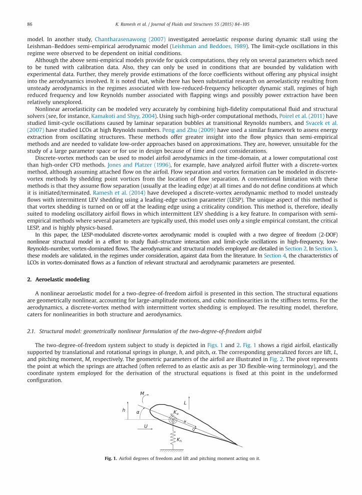
The two-degree-of-freedom system subject to study is depicted in Figs. 1 and 2. Fig. 1 shows a rigid airfoil, elasticallysupported by translational and rotational springs in plunge, h, and pitch, α. The corresponding generalized forces are lift, L,and pitching moment, M, respectively. The geometric parameters of the airfoil are illustrated in Fig. 2. The pivot representsthe point at which the springs are attached (often referred to as elastic axis as per 3D flexible-wing terminology), and thecoordinate system employed for the derivation of the structural equations is fixed at this point in the undeformedconfiguration.

Fig. 1. Airfoil degrees of freedom and lift and pitching moment acting on it.

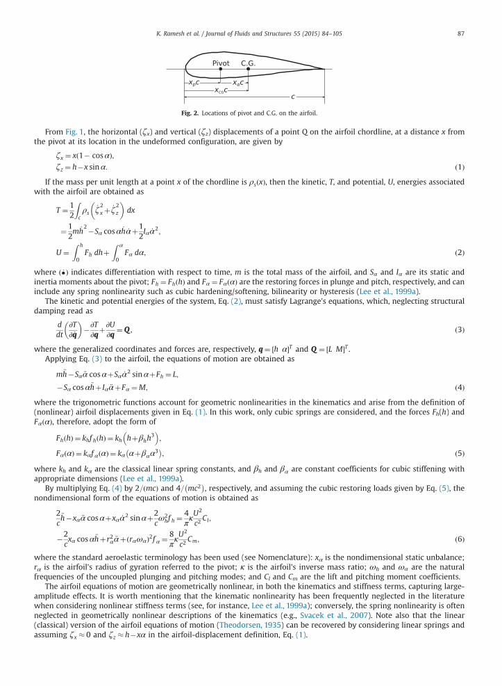
Fig. 2. Locations of pivot and C.G. on the airfoil.

K. Ramesh et al. / Journal of Fluids and Structures 55 (2015) 84–105 87

From Fig. 1, the horizontal (ζx) and vertical (ζz) displacements of a point Q on the airfoil chordline, at a distance x fromthe pivot at its location in the undeformed configuration, are given by

ζx ¼ xð1� cosαÞ;ζz ¼ h�x sinα: ð1Þ

If the mass per unit length at a point x of the chordline is ρsðxÞ, then the kinetic, T, and potential, U, energies associatedwith the airfoil are obtained as

T ¼ 12

Zcρs

_ζ2x þ _ζ

2z

� �dx

¼ 12m _h

2�Sα cosα _h _αþ12Iα _α2;

U ¼Z h

0Fh dhþ

Z α

0Fα dα; ð2Þ

where ð _�Þ indicates differentiation with respect to time, m is the total mass of the airfoil, and Sα and Iα are its static andinertia moments about the pivot; Fh ¼ FhðhÞ and Fα ¼ FαðαÞ are the restoring forces in plunge and pitch, respectively, and caninclude any spring nonlinearity such as cubic hardening/softening, bilinearity or hysteresis (Lee et al., 1999a).

The kinetic and potential energies of the system, Eq. (2), must satisfy Lagrange's equations, which, neglecting structuraldamping read as

ddt

∂T∂ _q

� ��∂T∂q

þ∂U∂q

¼Q ; ð3Þ

where the generalized coordinates and forces are, respectively, q¼ ½h α�T and Q ¼ ½L M�T .Applying Eq. (3) to the airfoil, the equations of motion are obtained as

m €h�Sα €α cosαþSα _α2 sinαþFh ¼ L;

�Sα cosα €hþ Iα €αþFα ¼M; ð4Þwhere the trigonometric functions account for geometric nonlinearities in the kinematics and arise from the definition of(nonlinear) airfoil displacements given in Eq. (1). In this work, only cubic springs are considered, and the forces Fh(h) andFαðαÞ, therefore, adopt the form of

FhðhÞ ¼ khf hðhÞ ¼ kh hþβhh3

� �;

FαðαÞ ¼ kαf αðαÞ ¼ kα αþβαα3� �; ð5Þ

where kh and kα are the classical linear spring constants, and βh and βα are constant coefficients for cubic stiffening withappropriate dimensions (Lee et al., 1999a).

By multiplying Eq. (4) by 2=ðmcÞ and 4= mc2� �

, respectively, and assuming the cubic restoring loads given by Eq. (5), thenondimensional form of the equations of motion is obtained as

2c€h�xα €α cosαþxα _α2 sinαþ2

cω2

hf h ¼4πκU2

c2Cl;

�2cxα cosα €hþr2α €αþ rαωαð Þ2f α ¼

8πκU2

c2Cm; ð6Þ

where the standard aeroelastic terminology has been used (see Nomenclature): xα is the nondimensional static unbalance;rα is the airfoil's radius of gyration referred to the pivot; κ is the airfoil's inverse mass ratio; ωh and ωα are the naturalfrequencies of the uncoupled plunging and pitching modes; and Cl and Cm are the lift and pitching moment coefficients.

The airfoil equations of motion are geometrically nonlinear, in both the kinematics and stiffness terms, capturing large-amplitude effects. It is worth mentioning that the kinematic nonlinearity has been frequently neglected in the literaturewhen considering nonlinear stiffness terms (see, for instance, Lee et al., 1999a); conversely, the spring nonlinearity is oftenneglected in geometrically nonlinear descriptions of the kinematics (e.g., Svacek et al., 2007). Note also that the linear(classical) version of the airfoil equations of motion (Theodorsen, 1935) can be recovered by considering linear springs andassuming ζx � 0 and ζz � h�xα in the airfoil-displacement definition, Eq. (1).

Fig. 3. Depiction of time-stepping scheme.

Fig. 4. Airfoil velocities and pivot location.

K. Ramesh et al. / Journal of Fluids and Structures 55 (2015) 84–10588

2.2. Aerodynamic model: discrete-vortex model with intermittent LEV shedding

The aerodynamic model used in the current work is a recently developed discrete vortex method with a novel sheddingcriterion that modulates intermittent vortex shedding from the leading edge. The shedding criterion, governed by amaximum allowable leading-edge suction, is based on the critical value of a leading-edge suction parameter (LESP). Thissection briefly describes the main elements of the LESP-modulated discrete-vortex method (LDVM). The interested readermay refer to Ramesh et al. (2013, 2014) for further details.

2.2.1. Large-angle unsteady thin-airfoil theoryAt the foundation of the LDVM is a large-angle unsteady thin-airfoil theory detailed in Ramesh et al. (2013). This theory is

based on the time-stepping formulation given by Katz and Plotkin (2000), but eliminates the traditional small-angleassumptions in thin-airfoil theory which may be invalid in flows of current interest. At each time step, a discrete vortex isshed from the airfoil trailing edge (referred to as TEV) as depicted in Fig. 3. When dictated by the LESP-based sheddingcriterion (Section 2.2.2), a discrete vortex is also shed from the leading edge at some time steps. The vorticity distributionover the airfoil at any given time step is taken to be a Fourier series truncated to r terms:

γ θ� �¼ 2U A0

1þ cosθsinθ

þXr

i ¼ 1

Ai sin iθ� �" #

; ð7Þ

where the transformation variable θ relates to the chordwise coordinate as: x¼ cð1� cosθÞ=2, with x measured from theleading edge; that is, 0rxrc and 0rθrπ. A0, A1, …, Ar are the time-dependent Fourier coefficients, and U is thefreestream velocity. The Kutta condition (zero vorticity at the trailing-edge) is enforced implicitly through the form of theFourier series. The Fourier coefficients are calculated by enforcing the boundary condition of zero normal flow through theairfoil camberline as

A0 ¼ �1π

Z π

0

WðθÞU

dθ; ð8Þ

Ai ¼2π

Z π

0

WðθÞU

cos iθ� �

dθ; ð9Þ

where WðθÞ is the induced velocity normal to the airfoil camberline. This value is calculated from components of motionkinematics, depicted in Fig. 4, and induced velocities from all vortices in the flowfield.

When there is no LEV shedding in a time step, the only unknown is the strength of the last-shed trailing-edge vortex andthis is calculated iteratively such that Kelvin's circulation condition is satisfied (Ramesh et al., 2013). If a TEV and LEV areboth shed in a time step, their strengths are determined as discussed in Section 2.2.2.

K. Ramesh et al. / Journal of Fluids and Structures 55 (2015) 84–105 89

2.2.2. LESP criterion for LEV formation and sheddingThe LESP is a measure of the suction peak at the leading edge, which in turn is caused by the stagnation point moving

away from the leading edge when the airfoil is at an angle of attack. From Garrick (1937) and von Karman and Burgers(1935), the suction at the leading edge in potential flow may be expressed as

S¼ limx-LE

12γ xð Þ ffiffiffi

xp

: ð10Þ

Evaluating using the current formulation, S¼ ffiffiffic

pUA0. The leading edge suction parameter is defined as a nondimensional

value of suction at the leading edge, and is hence simply set equal to the first coefficient from Eq. (7), A0.As noted by Katz (1981), real airfoils have rounded leading edges which can support some suction even when the

stagnation point is away from the airfoil leading edge. The amount of suction that can be supported is a characteristic of theairfoil shape and Reynolds number of operation. When these quantities are constant, it was shown in Ramesh et al. (2014)that initiation of LEV formation always occurred at the same value of LESP regardless of motion kinematics and history. Thisthreshold value of LESP, which is a function of the airfoil shape and Reynolds number, is termed the critical LESP. This value,for any given airfoil and Reynolds number (and other specific operating conditions such as freestream turbulence and thepresence of roughness), can be obtained from CFD or experimental predictions for a single motion (Ramesh et al., 2014), andcan then be used for any other motion to predict LEV formation. In the LDVM model, a discrete vortex is shed is from theleading edge at those time steps when the instantaneous LESP (A0 value) is greater than the critical LESP value. The strengthof the LEV is determined such that the instantaneous LESP value, which would have otherwise exceeded the critical LESPvalue, is made equal to the latter. This condition, along with Kelvin's condition, is used to determine shed vortex strengthsiteratively in time steps where both TEV and LEV are shed.

2.2.3. Vortex method detailsIn the current approach, the vortex-core model proposed by Vatistas et al. (1991), which gives an excellent

approximation to the Lamb–Oseen vortex, is used to represent the discrete vortices as vortex blobs. Using this core modelwith order two, the velocities induced at X and Z (u and w) by the kth vortex in the X and Z directions are

u;w½ � ¼ γk2π

Z�Zkð Þ; Xk�Xð Þ½ �ffiffiffiffiffiffiffiffiffiffiffiffiffiffiffiffiffiffiffiffiffiffiffiffiffiffiffiffiffiffiffiffiffiffiffiffiffiffiffiffiffiffiffiffiffiffiffiffiffiffiffiffiffiffiffiffiffiffiffiffiffiffiX�Xkð Þ2þ Z�Zkð Þ2

h i2þv4core

r : ð11Þ

A nondimensional time stepΔtn ¼ΔtU=c¼ 0:015 is used for all simulations presented in this paper. Hald (1979) has proved thatthe vortex-blob method is convergent (stable when run over long periods) so long as the vortex-core radius is larger than theaverage spacing between vortices. The average spacing between the vortices, d, is calculated as d¼ cΔtn. The vortex core radius istaken to be approximately 1.3 times the average spacing between the vortices (as suggested by Leonard, 1980): vcore ¼ 0:02c.Convergence studies have been performed during the development of this method, and the numerical parameters have beenselected such that the simulation results are not improved by either increasing or decreasing their values.

To control vortex count, and thus limit the computational cost, vortices which are a distance greater than ten chordlengths from the airfoil are deleted. When vortices are deleted from the domain, Kelvin's circulation condition which is usedto iterate for shed vortex strengths is updated accordingly. Test simulations showed that results did not change when thecutoff distance was increased beyond ten chord lengths, implying that the velocity induced by vortices at a distance greaterthan ten chord lengths is negligible in comparison with other velocities acting on the airfoil.

At each time-step, all the free vortices in the flowfield are convected by the net local velocity induced at their centers.A first-order time-stepping procedure is used for updating vortex positions, since no significant change in accuracy wasobserved by using higher-order methods.

2.2.4. Forces and moment on airfoilThe forces and moment on the airfoil are derived in detail in Ramesh et al. (2014) and are outlined briefly here. The two

forces on the airfoil are the normal force and leading-edge suction force, given by

FN ¼ ρπcU U cosαþ _h sinα� �

A0þ12A1

� �þc

34_A0 þ

14_A1 þ

18_A2

� �

þρZ c

0

∂ϕlev

∂x

� �þ ∂ϕtev

∂x

� �� �γ xð Þ dx; ð12Þ

FS ¼ ρπcU2ðA0Þ2: ð13ÞThe moment about an arbitrary reference point, xref, is given by

M¼ xref FN�ρπc2U U cosαþ _h sinα� � 1

4A0þ

14A1�

18A2

� �þc

716

_A0 þ1164

_A1 þ116

_A2 �164

_A3

� �

�ρZ c

0

∂ϕlev

∂x

� �þ ∂ϕlev

∂x

� �� �γ xð Þx dx: ð14Þ

K. Ramesh et al. / Journal of Fluids and Structures 55 (2015) 84–10590

The force coefficients (CN and CS) are evaluated by dividing the forces by 12ρU

2c and the moment coefficient (Cm) isobtained as M=12ρU

2c2. The lift and drag coefficients (Cl and Cd) are calculated using components of normal and leading-edgesuction forces. The time derivatives of the Fourier coefficients in the forces and pitching moment (Eqs. (12)–(14)) arise fromthe apparent-mass contribution which is very significant for high-reduced-frequency motion.

2.2.5. Limitations of the aerodynamics modelAs shown in Ramesh et al. (2014), the predictions from the current LDVM are in reasonable, and sometimes excellent,

agreement with those from CFD and experiments. Because the LDVM does not model thick or separated boundary layers,the method is restricted to motions where the LEV formation occurs without being accompanied by significant trailing-edgeseparation or stall. For most rounded-leading-edge airfoils, the LDVM is most reliable for high-reduced-frequency motions,with k40:4. In the current work, all LCOs studied in Section 4 have k40:6.

Another disadvantage, which is characteristic of vortex methods, is the exponential increase in computational time withnumber of vortices in the flow field (Oðn2Þ). Fast summation methods (Carrier et al., 1988), amalgamation of vortices, ordeletion of vortices that exit the field of interest could be used to control the vortex count. As mentioned previously, vorticesthat are at a distance greater than ten chord lengths from the airfoil are deleted in the current implementation.

2.3. Aero-structural coupling

The coupling between the structural and aerodynamic models is described next. The structural model is governed bysecond-order ordinary differential equations in continuous time, whereas the aerodynamic model is naturally written indiscrete time. In order to couple both models, the structural equations are integrated in time using a three-step Adam–

Bashforth scheme (Butcher, 2008), whereby the generalized coordinates and their derivatives (pitch, plunge andcorresponding rates) are marched as

q_q

( )nþ1

¼q_q

( )n

þΔt12

23_q€q

( )n

�16_q€q

( )n�1

þ5_q€q

( )n�224

35; ð15Þ

with n being the time step at which states are evaluated. This is an explicit time-marching scheme in which onlyinformation from previous time steps is required.

The aero-structural integration is based on a loosely coupled approach in which information is exchanged at each timestep, but no subiterations are included. This scheme has been chosen due to the first-order, explicit nature of theaerodynamic model, and because it has shown excellent convergence properties for the appropriate selection of simulationparameters. The main steps of the process are briefly summarized below:

1.

Based on the geometry and velocities at time step n, the aerodynamic loads are computed from the discrete-vortexmethod with the corresponding vorticity distribution, including leading-edge vortices when applicable.

2.

These aerodynamic loads at time step n are applied to the structural equations, Eq. (6), which are solved to yield theacceleration values €h

nand €αn.

3.

From the Adam–Bashforth integration scheme, Eq. (15), the structural states (plunge, pitch and corresponding rates) attime step nþ1 are determined.

4.

The procedure is repeated from step 1.

The aeroelastic coupling and integrations are also depicted in a flowchart in Fig. 5, with a detailed description of how thediscrete-vortex method operates.

3. Validation against previous work

Validation of the current method with linear aerodynamics is presented for aeroelastic predictions: using linear structures inSection 3.1 and using nonlinear structures in Section 3.2. Because there is almost no suitable data in the literature for passiveairfoil aeroelasticity in high-frequency, LEV-dominated flows, validation of the nonlinear aerodynamics is presented forprescribed kinematics in Section 3.3.

3.1. Validation for linear aerodynamics and linear structures: onset of linear flutter for the classical 2-DOF airfoil

The classical two-degree-of-freedom linear flutter problem is used to validate the aeroelastic model developed in thiswork. The LEV shedding in the aerodynamic model is “turned off” by setting the critical LESP to a very high value of 5.0. Theaerodynamic model thus provides a potential-flow solution with attached flow at the leading edge, enabling validation ofthe method with linear-flutter-onset data. Since the current method is based in the time domain, flutter velocities areidentified as those above which divergent oscillations occur.

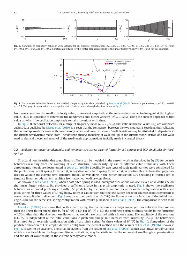
As an illustration of how the oscillation characteristics vary with velocity, Fig. 6 shows the variations of α with tn at threenondimensional velocity values (Un ¼U=ωαc) for an example configuration. It is seen that the oscillatory behavior changes

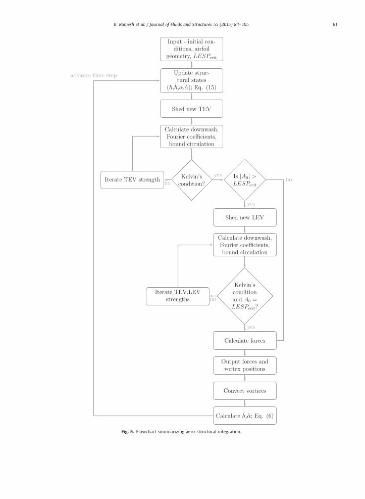
Fig. 5. Flowchart summarizing aero-structural integration.

K. Ramesh et al. / Journal of Fluids and Structures 55 (2015) 84–105 91

0 800−10

0

10

t*

α (d

eg)

0 800−10

0

10

t*

α (d

eg)

0 800−10

0

10

t*

α (d

eg)

Fig. 6. Variation of oscillatory behavior with velocity for an example configuration (xp¼0.35, κ¼ 0:05, rα ¼ 0:5, xα ¼ 0:2 and ω ¼ 1:0). Left to right:Un ¼ 0:62, Un ¼ 0:64, and Un ¼ 0:66. Constant amplitude for the center case corresponds to the linear flutter velocity of Un

F ¼ 0:64 for this example.

Fig. 7. Flutter-onset velocities from current method compared against data published by Murua et al. (2010). Structural parameters: xp¼0.35, κ¼ 0:05,rα ¼ 0:5. The gray circle contains the data point which is determined through the illustration in Fig. 6.

K. Ramesh et al. / Journal of Fluids and Structures 55 (2015) 84–10592

from convergent for the smallest velocity value, to constant amplitude at the intermediate value, to divergent at the highestvalue. Thus, it is possible to determine the nondimensional flutter velocity (Un

F ¼UF=ωαc) using the current approach as thatvalue at which the oscillation amplitude remains invariant with time.

In Fig. 7, flutter-onset velocities for a range of frequency ratios (ω ¼ωh=ωα) and static unbalance values (xα) are comparedagainst data published by Murua et al. (2010). It is seen that the comparison between the two methods is excellent, thus validatingthe current approach for cases with linear aerodynamics and linear structures. Small deviations may be attributed to departures inthe current aerodynamic model from Theodorsen's theory: modeling of wake roll-up in the current model instead of a flat wakeused in classical theory and removal of the small-angle approximations typically made in classical theory.

3.2. Validation for linear aerodynamics and nonlinear structures: onset of flutter for soft springs and LCO amplitudes for hardsprings

Structural nonlinearities due to nonlinear stiffness can be modeled in the current work as described in Eq. (5). Aeroelasticbehaviors resulting from the coupling of such structural nonlinearity, by use of different cubic stiffnesses, with linearaerodynamic models are documented in Lee et al. (1999b). Specifically, two types of cubic nonlinearities were considered forthe pitch spring: a soft spring for which βα is negative and a hard spring for which βα is positive. Results from that paper areused to validate the current aero-structural model. As was done in the earlier subsection, LEV shedding is “turned off” tosimulate linear aerodynamics resulting from attached leading-edge flows.

As shown in Lee et al. (1999b), when a soft pitch spring is used, divergent oscillations can occur even at velocities belowthe linear flutter velocity, UF, provided a sufficiently large initial pitch amplitude is used. Fig. 8 shows the oscillatorybehavior for an initial pitch angle of αð0Þ ¼ 51 predicted by the current method for an example configuration with a softpitch spring for three values of Un=Un

F below unity. It can be seen that the oscillatory behavior changes from convergent toconstant-amplitude to divergent. Fig. 9 compares the prediction of Un=Un

F for flutter onset as a function of the initial pitchangle, αð0Þ, for the same soft-spring configuration with results published in Lee et al. (1999b). The comparison is seen to beexcellent.

Lee et al. (1999b) also show that, with a hard spring, the oscillations are always convergent for velocities that are lessthan the linear flutter speed, that is, for Un=Un

Fo1:0. For Un=Un

F41:0, the nonlinear spring stiffness results in the formationof LCOs rather than the divergent oscillations that would have occurred with a linear spring. The amplitude of the resultingLCO, αA, is independent of the initial conditions in pitch and plunge, but increases with increasing Un=Un

F . The behavior isillustrated for an example configuration with a hard pitch spring for three values of Un=Un

F in Fig. 10. Comparison of thepredicted variation of LCO amplitude with Un=Un

F from the current method with the results of Lee et al. (1999b), shown inFig. 11, is seen to be excellent. The small deviations from the results of Lee et al. (1999b) (which uses linear aerodynamics),which are noticeable in the larger-amplitude oscillations, may be attributed to the removal of small-angle approximationsand the use of wake rollup in the current aerodynamic model.

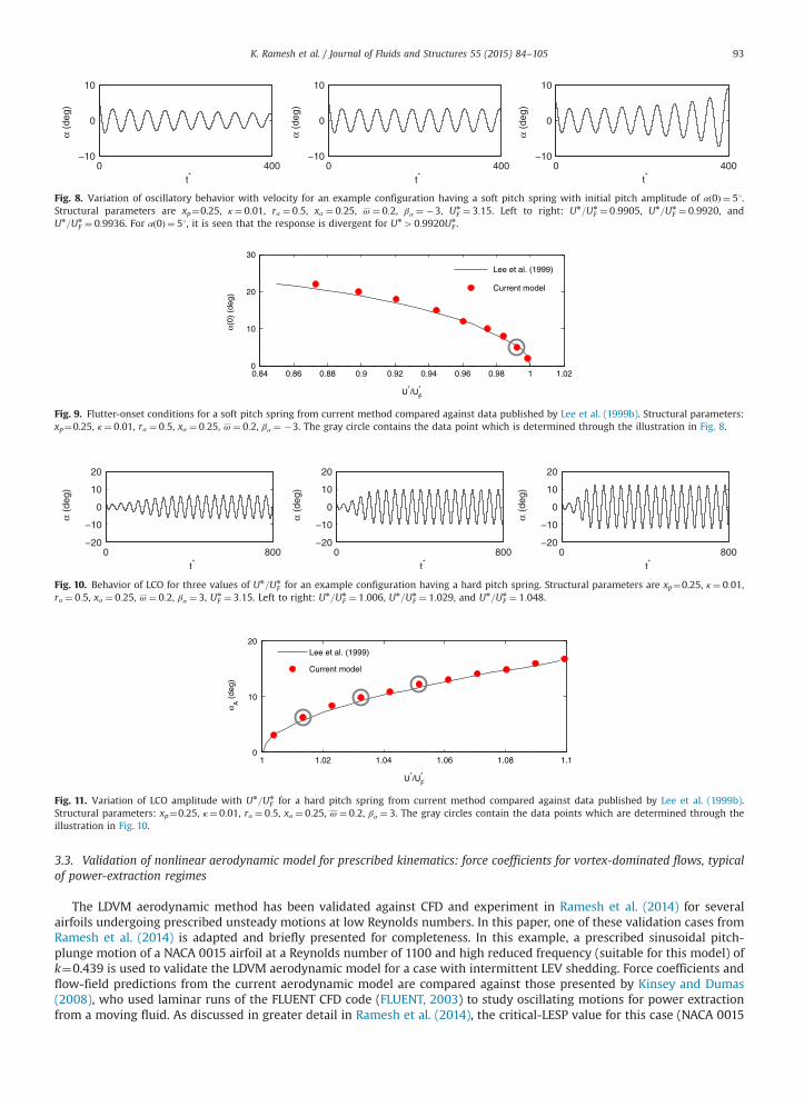
Fig. 9. Flutter-onset conditions for a soft pitch spring from current method compared against data published by Lee et al. (1999b). Structural parameters:xp¼0.25, κ¼ 0:01, rα ¼ 0:5, xα ¼ 0:25, ω ¼ 0:2, βα ¼ �3. The gray circle contains the data point which is determined through the illustration in Fig. 8.

Fig. 10. Behavior of LCO for three values of Un=Un

F for an example configuration having a hard pitch spring. Structural parameters are xp¼0.25, κ¼ 0:01,rα ¼ 0:5, xα ¼ 0:25, ω ¼ 0:2, βα ¼ 3, Un

F ¼ 3:15. Left to right: Un=Un

F ¼ 1:006, Un=Un

F ¼ 1:029, and Un=Un

F ¼ 1:048.

Fig. 8. Variation of oscillatory behavior with velocity for an example configuration having a soft pitch spring with initial pitch amplitude of αð0Þ ¼ 51.Structural parameters are xp¼0.25, κ¼ 0:01, rα ¼ 0:5, xα ¼ 0:25, ω ¼ 0:2, βα ¼ �3, Un

F ¼ 3:15. Left to right: Un=Un

F ¼ 0:9905, Un=Un

F ¼ 0:9920, andUn=Un

F ¼ 0:9936. For αð0Þ ¼ 51, it is seen that the response is divergent for Un40:9920Un

F .

Fig. 11. Variation of LCO amplitude with Un=Un

F for a hard pitch spring from current method compared against data published by Lee et al. (1999b).Structural parameters: xp¼0.25, κ¼ 0:01, rα ¼ 0:5, xα ¼ 0:25, ω ¼ 0:2, βα ¼ 3. The gray circles contain the data points which are determined through theillustration in Fig. 10.

K. Ramesh et al. / Journal of Fluids and Structures 55 (2015) 84–105 93

3.3. Validation of nonlinear aerodynamic model for prescribed kinematics: force coefficients for vortex-dominated flows, typicalof power-extraction regimes

The LDVM aerodynamic method has been validated against CFD and experiment in Ramesh et al. (2014) for severalairfoils undergoing prescribed unsteady motions at low Reynolds numbers. In this paper, one of these validation cases fromRamesh et al. (2014) is adapted and briefly presented for completeness. In this example, a prescribed sinusoidal pitch-plunge motion of a NACA 0015 airfoil at a Reynolds number of 1100 and high reduced frequency (suitable for this model) ofk¼0.439 is used to validate the LDVM aerodynamic model for a case with intermittent LEV shedding. Force coefficients andflow-field predictions from the current aerodynamic model are compared against those presented by Kinsey and Dumas(2008), who used laminar runs of the FLUENT CFD code (FLUENT, 2003) to study oscillating motions for power extractionfrom a moving fluid. As discussed in greater detail in Ramesh et al. (2014), the critical-LESP value for this case (NACA 0015

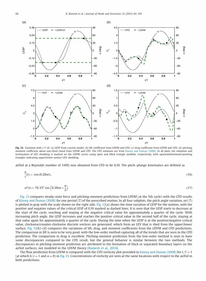
Fig. 12. Variation with t=T of: (a) LESP from current model, (b) lift coefficient from LDVM and CFD, (c) drag coefficient from LDVM and CFD, (d) pitchingmoment coefficient about one-third chord from LDVM and CFD. The CFD solutions are from Kinsey and Dumas (2008). In all plots, the initiation andtermination of LEV shedding is marked on the LDVM curves using open and filled triangle symbols, respectively, with upward/downward-pointingtriangles indicating upper/lower-surface LEV shedding.

K. Ramesh et al. / Journal of Fluids and Structures 55 (2015) 84–10594

airfoil at a Reynolds number of 1100) was obtained from CFD to be 0.19. The pitch–plunge kinematics are defined as

hctð Þ ¼ cos 0:28πtð Þ; ð16Þ

αo tð Þ ¼ 76:33o cos 0:28πtþπ2

� �: ð17Þ

Fig. 12 compares steady-state force and pitching-moment predictions from LDVM (at the 5th cycle) with the CFD resultsof Kinsey and Dumas (2008) for one period (T) of the prescribed motion. In all four subplots, the pitch angle variation, αðt=TÞis plotted in gray with the scale shown on the right side. Fig. 12(a) shows the time variation of LESP for the motion, with thepositive and negative values of the critical LESP of 0.19 marked as dashed lines. It is seen that the LESP starts to decrease atthe start of the cycle, reaching and staying at the negative critical value for approximately a quarter of the cycle. Withincreasing pitch angle, the LESP increases and reaches the positive critical value in the second half of the cycle, staying atthat value again for approximately a quarter of the cycle. During the time when the LESP is at the positive/negative criticalvalue, clockwise/counter-clockwise discrete vortices are generated, which form an LEV that is shed from the upper/lowersurface. Fig. 12(b)–(d) compares the variations of lift, drag, and moment coefficients from the LDVM and CFD predictions.The comparison in lift is seen to be very good, with the low-order method capturing all of the trends that are seen in the CFDprediction. The comparison in drag is excellent. Pitching-moment prediction from the low-order method is seen to havesome discrepancies compared to the CFD result, but the general behavior is similar between the two methods. Thediscrepancies in pitching-moment prediction are attributed to the formation of thick or separated boundary layers on theairfoil surfaces, not modeled in the LDVM theory (Ramesh et al., 2014).

The flow prediction from LDVM is compared with the CFD vorticity plot provided in Kinsey and Dumas (2008) for t=T ¼ 1(at which h=c¼ 1 and α¼ 0) in Fig. 13. Concentrations of vorticity are seen at the same locations with respect to the airfoil inboth predictions.

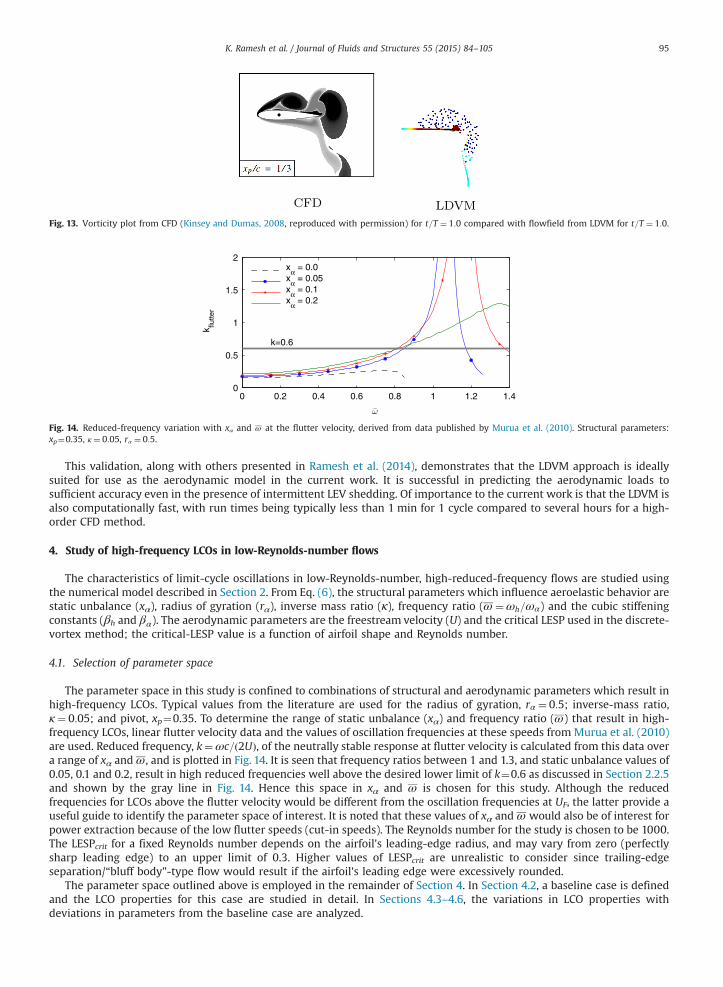
Fig. 13. Vorticity plot from CFD (Kinsey and Dumas, 2008, reproduced with permission) for t=T ¼ 1:0 compared with flowfield from LDVM for t=T ¼ 1:0.

Fig. 14. Reduced-frequency variation with xα and ω at the flutter velocity, derived from data published by Murua et al. (2010). Structural parameters:xp¼0.35, κ¼ 0:05, rα ¼ 0:5.

K. Ramesh et al. / Journal of Fluids and Structures 55 (2015) 84–105 95

This validation, along with others presented in Ramesh et al. (2014), demonstrates that the LDVM approach is ideallysuited for use as the aerodynamic model in the current work. It is successful in predicting the aerodynamic loads tosufficient accuracy even in the presence of intermittent LEV shedding. Of importance to the current work is that the LDVM isalso computationally fast, with run times being typically less than 1 min for 1 cycle compared to several hours for a high-order CFD method.

4. Study of high-frequency LCOs in low-Reynolds-number flows

The characteristics of limit-cycle oscillations in low-Reynolds-number, high-reduced-frequency flows are studied usingthe numerical model described in Section 2. From Eq. (6), the structural parameters which influence aeroelastic behavior arestatic unbalance (xα), radius of gyration (rα), inverse mass ratio (κ), frequency ratio (ω ¼ωh=ωα) and the cubic stiffeningconstants (βh and βα). The aerodynamic parameters are the freestream velocity (U) and the critical LESP used in the discrete-vortex method; the critical-LESP value is a function of airfoil shape and Reynolds number.

4.1. Selection of parameter space

The parameter space in this study is confined to combinations of structural and aerodynamic parameters which result inhigh-frequency LCOs. Typical values from the literature are used for the radius of gyration, rα ¼ 0:5; inverse-mass ratio,κ ¼ 0:05; and pivot, xp¼0.35. To determine the range of static unbalance (xα) and frequency ratio (ω) that result in high-frequency LCOs, linear flutter velocity data and the values of oscillation frequencies at these speeds from Murua et al. (2010)are used. Reduced frequency, k¼ωc=ð2UÞ, of the neutrally stable response at flutter velocity is calculated from this data overa range of xα andω, and is plotted in Fig. 14. It is seen that frequency ratios between 1 and 1.3, and static unbalance values of0.05, 0.1 and 0.2, result in high reduced frequencies well above the desired lower limit of k¼0.6 as discussed in Section 2.2.5and shown by the gray line in Fig. 14. Hence this space in xα and ω is chosen for this study. Although the reducedfrequencies for LCOs above the flutter velocity would be different from the oscillation frequencies at UF, the latter provide auseful guide to identify the parameter space of interest. It is noted that these values of xα and ω would also be of interest forpower extraction because of the low flutter speeds (cut-in speeds). The Reynolds number for the study is chosen to be 1000.The LESPcrit for a fixed Reynolds number depends on the airfoil's leading-edge radius, and may vary from zero (perfectlysharp leading edge) to an upper limit of 0.3. Higher values of LESPcrit are unrealistic to consider since trailing-edgeseparation/“bluff body”-type flow would result if the airfoil's leading edge were excessively rounded.

The parameter space outlined above is employed in the remainder of Section 4. In Section 4.2, a baseline case is definedand the LCO properties for this case are studied in detail. In Sections 4.3–4.6, the variations in LCO properties withdeviations in parameters from the baseline case are analyzed.

Table 1Base parameter set used to study LCO characteristics in high-frequency, low-Reynolds-number flows.

Parameter Symbol Value

Static unbalance xα 0.05Radius of gyration rα 0.5Inverse mass ratio κ 0.05Frequency ratio ω ¼ωh=ωα 1.0Cubic stiffening – pitch βα 0.0Cubic stiffening – plunge βh 0.0Flutter velocity Un

F 0.359Freestream velocity Un 1:3Un

F ¼ 0:4667Critical LESP LESPcrit 0.11Initial conditions – pitch αð0Þ, _αð0Þ αð0Þ ¼ 10○ , _αð0Þ ¼ 0Initial conditions – plunge hð0Þ, _hð0Þ hð0Þ ¼ _hð0Þ ¼ 0

K. Ramesh et al. / Journal of Fluids and Structures 55 (2015) 84–10596

4.2. Baseline case for the four-part parametric study

The base parameter set for this research is derived from the considerations detailed above and is listed in Table 1. Valuesof xα ¼ 0:05 and ω ¼ 1:0 are used, for which the linear flutter velocity from Murua et al. (2010) is Un

F ¼ 0:359. The baselinefreestream velocity is taken to be 1.3 times the linear flutter velocity. A 2.3%-thick flat-plate airfoil with a semi-circularleading edge is considered, and the critical LESP value for this airfoil at Re¼1000 is 0.11 as calibrated from CFD in Rameshet al. (2014). The springs are assumed to have linear stiffness in the baseline configuration. The effect of cubic stiffening isanalyzed in Section 4.4.

The airfoil's aeroelastic response for the base parameter set listed in Table 1 is shown in Fig. 15. The pitch and plungeamplitudes increase from their initial values and reach a limiting value as shown in the insets of Fig. 15(a) and (b). Thevariations of pitch and plunge with time (nondimensional), after limit-cycle oscillations are reached, are plotted in Fig. 15(a)and (b). It is apparent and is further established below, that the response is single-period. A single time period of the airfoil'sresponse is enclosed by dashed lines. Fig. 15(c) shows the variation of LESP with tn. This parameter controls leading-edgevortex formation in the discrete-vortex model. From the figure, it is seen that during one period, the LESP value reaches thepositive and negative critical LESP values once in each cycle. This behavior corresponds to one LEV being formed on theairfoil's upper surface followed by another on the lower surface in one period. The time instants at which the LESP valuesoverlap with the critical LESP value in the figure mark the instants at which discrete vortices are released from the leadingedge in the discrete-vortex model. The lift, drag and pitching moment coefficients calculated from the aerodynamic modelare shown in Fig. 15(d)–(f). Fig. 15(g) and (h) is phase-plane and power spectral density (PSD) plots of the response,respectively. The horizontal axis of the PSD plot is reduced frequency (k). The phase-plane and PSD plots further affirm thatthe limit-cycle oscillation is single period. The PSD plot shows the response reduced frequency to be approximately 1.08.Thus the airfoil oscillation ensuing from the chosen parameters is of high reduced frequency, where the flow is expected tobe dominated by leading-edge vortices and apparent-mass forces, and the aerodynamic model is expected to represent theflow physics well.

The steady-state and harmonic limit-cycle oscillations in pitch and plunge may be represented as

α¼ αA cos ð2ktnÞ; ð18Þ

hc¼ hA

ccos 2ktnþϕ

� �; ð19Þ

where αA and hA are the amplitudes of pitch and plunge, k is the reduced frequency of oscillation, and ϕ is the phase anglebetween pitch and plunge (with pitch leading plunge). For the LCO illustrated in Fig. 15, αA ¼ 16:6○, hA ¼ 0:128c, k¼1.08 andϕ¼ 49:1○.

Fig. 16(a)–(d) depicts the flow topology during one period of the LCO. As noted earlier, one LEV is shed over the airfoilupper surface, followed by another from the lower surface during one cycle. In (b) and (d) discrete-vortex shedding from theleading edge is observed on the upper and lower surfaces, respectively. In (a) and (c) the LEVs are seen convecting over theairfoil chord, on the lower and upper surfaces, respectively. Fig. 16(e) depicts the wake topology ensuing from the limit-cycleoscillation.

It is emphasized here that limit-cycle behavior in the baseline case described above is solely owing to the aerodynamicnonlinearity (LEV shedding). To demonstrate this point, Fig. 17(a) and (b) shows the pitch variation for the baseline case withand without the LEV shedding turned on in the aerodynamic model. It is clear that when the aerodynamic nonlinearity isnot present, no LCOs are seen and divergent flutter results as there are no nonlinearities in the structural model. Fig. 17(c)and (d) shows the variation in LESP for these two cases. When LEV shedding is enabled in the model, the LESP is bounded byLESPcrit, thereby resulting in limit-cycle response where the pitch/plunge variation is bounded as well.

Fig. 15. Baseline case: limit-cycle response for the parameters listed in Table 1. Time variation of (a) pitch angle, (b) plunge per unit chord, (c) LESP, (d) liftcoefficient, (e) drag coefficient, (f) pitching moment coefficient. The dashed lines enclose one period of the LCO. (g) and (h) are phase-plane and PSD plots,respectively. Insets in (a) and (b) show long-time responses for pitch angle and plunge per unit chord.

K. Ramesh et al. / Journal of Fluids and Structures 55 (2015) 84–105 97

4.3. Parametric study A: effect of change in freestream velocity

The effect of freestreamvelocity on LCO characteristics is first illustrated by considering three representative values of Un=Un

F .Subsequently, the LCO behavior is presented for a wide range of Un=Un

F to show the resulting bifurcation characteristics. It isrecalled that, in this study, Un

F ¼ 0:359 is the linear flutter velocity from Murua et al. (2010).The LCO behaviors for the three velocities are presented in Fig. 18 by plotting in three columns the oscillations at three values

of Un=Un

F of 1.3, 1.8, and 2.3, from left to right. The top row shows the oscillations of α for a representative time window of335rtnr385. Also marked, using circle symbols, on the right side of each subplot of the top row are the α values

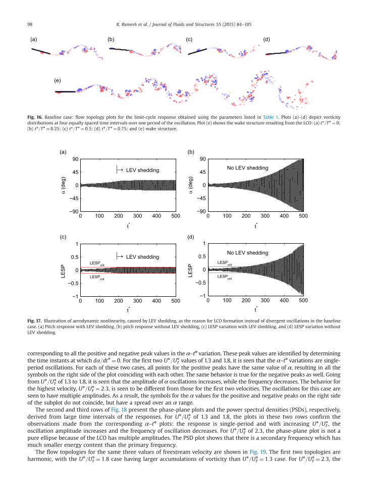
Fig. 16. Baseline case: flow topology plots for the limit-cycle response obtained using the parameters listed in Table 1. Plots (a)–(d) depict vorticitydistributions at four equally spaced time intervals over one period of the oscillation. Plot (e) shows the wake structure resulting from the LCO: (a) tn=Tn ¼ 0;(b) tn=Tn ¼ 0:25; (c) tn=Tn ¼ 0:5; (d) tn=Tn ¼ 0:75; and (e) wake structure.

0 100 200 300 400 500−90

−45

0

45

90

α (d

eg)

t*

→ LEV shedding

0 100 200 300 400 500−90

−45

0

45

90

α (d

eg)

t*

No LEV shedding

0 100 200 300 400 500−1

−0.5

0

0.5

1

LESPcrit

LESPcrit

LES

P

t*

→ LEV shedding

0 100 200 300 400 500−1

−0.5

0

0.5

1

LESPcrit

LESPcrit

LES

P

t*

No LEV shedding

Fig. 17. Illustration of aerodynamic nonlinearity, caused by LEV shedding, as the reason for LCO formation instead of divergent oscillations in the baselinecase. (a) Pitch response with LEV shedding, (b) pitch response without LEV shedding, (c) LESP variation with LEV shedding, and (d) LESP variation withoutLEV shedding.

K. Ramesh et al. / Journal of Fluids and Structures 55 (2015) 84–10598

corresponding to all the positive and negative peak values in the α–tn variation. These peak values are identified by determiningthe time instants at which dα=dtn ¼ 0. For the first two Un=Un

F values of 1.3 and 1.8, it is seen that the α–tn variations are single-period oscillations. For each of these two cases, all points for the positive peaks have the same value of α, resulting in all thesymbols on the right side of the plot coinciding with each other. The same behavior is true for the negative peaks as well. Goingfrom Un=Un

F of 1.3 to 1.8, it is seen that the amplitude of α oscillations increases, while the frequency decreases. The behavior forthe highest velocity, Un=Un

F ¼ 2:3, is seen to be different from those for the first two velocities. The oscillations for this case areseen to have multiple amplitudes. As a result, the symbols for the α values for the positive and negative peaks on the right sideof the subplot do not coincide, but have a spread over an α range.

The second and third rows of Fig. 18 present the phase-plane plots and the power spectral densities (PSDs), respectively,derived from large time intervals of the responses. For Un=Un

F of 1.3 and 1.8, the plots in these two rows confirm theobservations made from the corresponding α–tn plots: the response is single-period and with increasing Un=Un

F , theoscillation amplitude increases and the frequency of oscillation decreases. For Un=Un

F of 2.3, the phase-plane plot is not apure ellipse because of the LCO has multiple amplitudes. The PSD plot shows that there is a secondary frequency which hasmuch smaller energy content than the primary frequency.

The flow topologies for the same three values of freestream velocity are shown in Fig. 19. The first two topologies areharmonic, with the Un=Un

F ¼ 1:8 case having larger accumulations of vorticity than Un=Un

F ¼ 1:3 case. For Un=Un

F ¼ 2:3, the

Fig. 18. Parametric study A: comparison of LCO characteristics for different values of freestream velocity. Top row: time variation of pitch angle; middlerow: phase-plane plots; and bottom row: power-spectral density plots. Circles on the right side of each top-row subplot show the pitch valuescorresponding to all the positive and negative peaks in pitch angle-vs.-time variation.

K. Ramesh et al. / Journal of Fluids and Structures 55 (2015) 84–105 99

simulation shows a non-uniform wake structure with large transverse displacements of the vortical flow structures, whichreflects the multiple-amplitude LCO seen for this velocity.

Fig. 20(a) and (b) shows the variation in LCO characteristics over a large freestream-velocity range using bifurcation plotsof pitch and plunge, while Fig. 20(c) and (d) plots the variations of reduced frequency, k, and phase angle between pitch andplunge,ϕ. On the vertical axis of Fig. 20(a), peak values in pitch during the LCO are plotted. For each value of Un=Un

F , the peakα values, identified by determining the instances at which dα=dtn ¼ 0, are plotted as was done in Fig. 18. In a similar manner,the peak values of the plunge oscillations at various Un=Un

F are plotted in Fig. 20(b). The gray lines in 20(a) show thefreestream velocity values used for the illustrations in Figs. 18 and 19.

Fig. 20(a) and (b) is seen to have a bifurcation at a value of Un=Un

F slightly less than unity. While the bifurcation location inaeroelastic studies (Lee et al., 1999a) is typically at Un=Un

F ¼ 1, the slight shift from unity here is because the Un

F is defined asthe flutter velocity from Murua et al. (2010), rather than as the velocity at which the bifurcation occurs.

When the freestream velocity is lower than the flutter velocity, the solution is stable and converges to zero amplitude forall initial displacements. For values of nondimensional freestream velocity between the flutter speed and approximately2Un

F , the bifurcation plots show single-period behavior. This transition from stable equilibrium to limit-cycle oscillation atthe flutter speed appears to be a supercritical Hopf bifurcation (Lee et al., 1999a).

The amplitude of single-period LCOs is seen to increase with increasing freestream velocity. At nondimensional velocitiesgreater than 2Un

F , departure from single-period behavior is seen. The peaks of the response take on multiple values and theoscillation appears to be quasiperiodic, as gleaned from the PSD plot in Fig. 18. This type of transition from periodic to

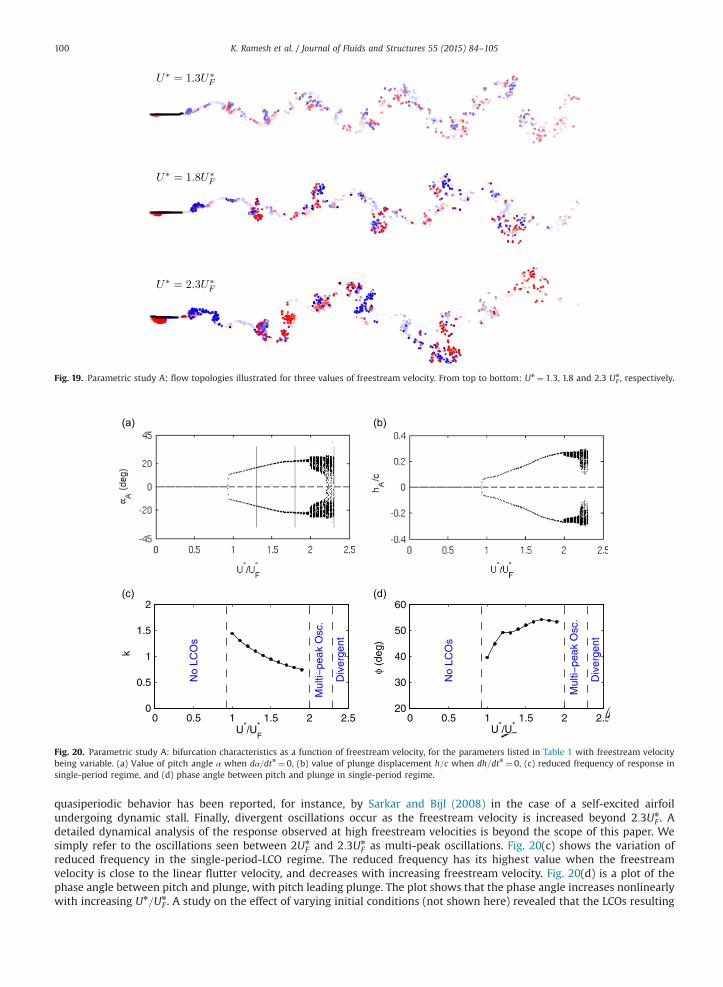
Fig. 19. Parametric study A: flow topologies illustrated for three values of freestream velocity. From top to bottom: Un ¼ 1:3, 1.8 and 2.3 Un

F , respectively.

Fig. 20. Parametric study A: bifurcation characteristics as a function of freestream velocity, for the parameters listed in Table 1 with freestream velocitybeing variable. (a) Value of pitch angle α when dα=dtn ¼ 0, (b) value of plunge displacement h=c when dh=dtn ¼ 0, (c) reduced frequency of response insingle-period regime, and (d) phase angle between pitch and plunge in single-period regime.

K. Ramesh et al. / Journal of Fluids and Structures 55 (2015) 84–105100

quasiperiodic behavior has been reported, for instance, by Sarkar and Bijl (2008) in the case of a self-excited airfoilundergoing dynamic stall. Finally, divergent oscillations occur as the freestream velocity is increased beyond 2:3Un

F . Adetailed dynamical analysis of the response observed at high freestream velocities is beyond the scope of this paper. Wesimply refer to the oscillations seen between 2Un

F and 2:3Un

F as multi-peak oscillations. Fig. 20(c) shows the variation ofreduced frequency in the single-period-LCO regime. The reduced frequency has its highest value when the freestreamvelocity is close to the linear flutter velocity, and decreases with increasing freestream velocity. Fig. 20(d) is a plot of thephase angle between pitch and plunge, with pitch leading plunge. The plot shows that the phase angle increases nonlinearlywith increasing Un=Un

F . A study on the effect of varying initial conditions (not shown here) revealed that the LCOs resulting

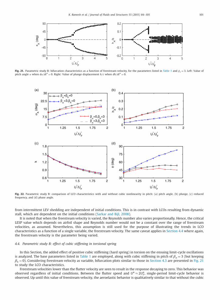
Fig. 21. Parametric study B: bifurcation characteristics as a function of freestream velocity, for the parameters listed in Table 1 and βα ¼ 3. Left: Value ofpitch angle α when dα=dtn ¼ 0. Right: Value of plunge displacement h=c when dh=dtn ¼ 0.

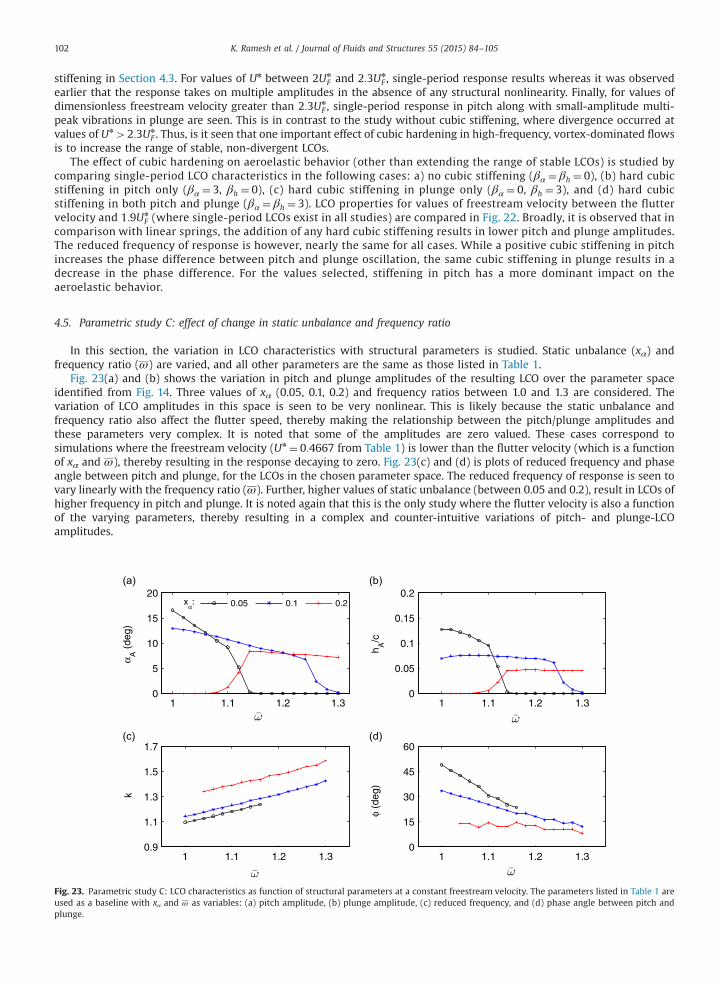
Fig. 22. Parametric study B: comparison of LCO characteristics with and without cubic nonlinearity in pitch: (a) pitch angle, (b) plunge, (c) reducedfrequency, and (d) phase angle.

K. Ramesh et al. / Journal of Fluids and Structures 55 (2015) 84–105 101

from intermittent LEV shedding are independent of initial conditions. This is in contrast with LCOs resulting from dynamicstall, which are dependent on the initial conditions (Sarkar and Bijl, 2008).

It is noted that when the freestream velocity is varied, the Reynolds number also varies proportionally. Hence, the criticalLESP value which depends on airfoil shape and Reynolds number would not be a constant over the range of freestreamvelocities, as assumed. Nevertheless, this assumption is still used for the purpose of illustrating the trends in LCOcharacteristics as a function of a single variable, the freestream velocity. The same caveat applies in Section 4.4 where again,the freestream velocity is the parameter being varied.

4.4. Parametric study B: effect of cubic stiffening in torsional spring

In this Section, the added effect of positive cubic stiffening (hard spring) in torsion on the ensuing limit-cycle oscillationsis analyzed. The base parameters listed in Table 1 are employed, along with cubic stiffening in pitch of βα ¼ 3 (but keepingβh ¼ 0). Considering freestream velocity as variable, bifurcation plots similar to those in Section 4.3 are presented in Fig. 21to study the LCO characteristics.

Freestream velocities lower than the flutter velocity are seen to result in the response decaying to zero. This behavior wasobserved regardless of initial conditions. Between the flutter speed and Un � 2Un

F , single-period limit-cycle behavior isobserved. Up until this value of freestream velocity, the aeroelastic behavior is qualitatively similar to that without the cubic

K. Ramesh et al. / Journal of Fluids and Structures 55 (2015) 84–105102

stiffening in Section 4.3. For values of Un between 2Un

F and 2:3Un

F , single-period response results whereas it was observedearlier that the response takes on multiple amplitudes in the absence of any structural nonlinearity. Finally, for values ofdimensionless freestream velocity greater than 2:3Un

F , single-period response in pitch along with small-amplitude multi-peak vibrations in plunge are seen. This is in contrast to the study without cubic stiffening, where divergence occurred atvalues of Un42:3Un

F . Thus, is it seen that one important effect of cubic hardening in high-frequency, vortex-dominated flowsis to increase the range of stable, non-divergent LCOs.

The effect of cubic hardening on aeroelastic behavior (other than extending the range of stable LCOs) is studied bycomparing single-period LCO characteristics in the following cases: a) no cubic stiffening (βα ¼ βh ¼ 0), (b) hard cubicstiffening in pitch only (βα ¼ 3, βh ¼ 0), (c) hard cubic stiffening in plunge only (βα ¼ 0, βh ¼ 3), and (d) hard cubicstiffening in both pitch and plunge (βα ¼ βh ¼ 3). LCO properties for values of freestream velocity between the fluttervelocity and 1:9Un

F (where single-period LCOs exist in all studies) are compared in Fig. 22. Broadly, it is observed that incomparison with linear springs, the addition of any hard cubic stiffening results in lower pitch and plunge amplitudes.The reduced frequency of response is however, nearly the same for all cases. While a positive cubic stiffening in pitchincreases the phase difference between pitch and plunge oscillation, the same cubic stiffening in plunge results in adecrease in the phase difference. For the values selected, stiffening in pitch has a more dominant impact on theaeroelastic behavior.

4.5. Parametric study C: effect of change in static unbalance and frequency ratio

In this section, the variation in LCO characteristics with structural parameters is studied. Static unbalance (xα) andfrequency ratio (ω) are varied, and all other parameters are the same as those listed in Table 1.

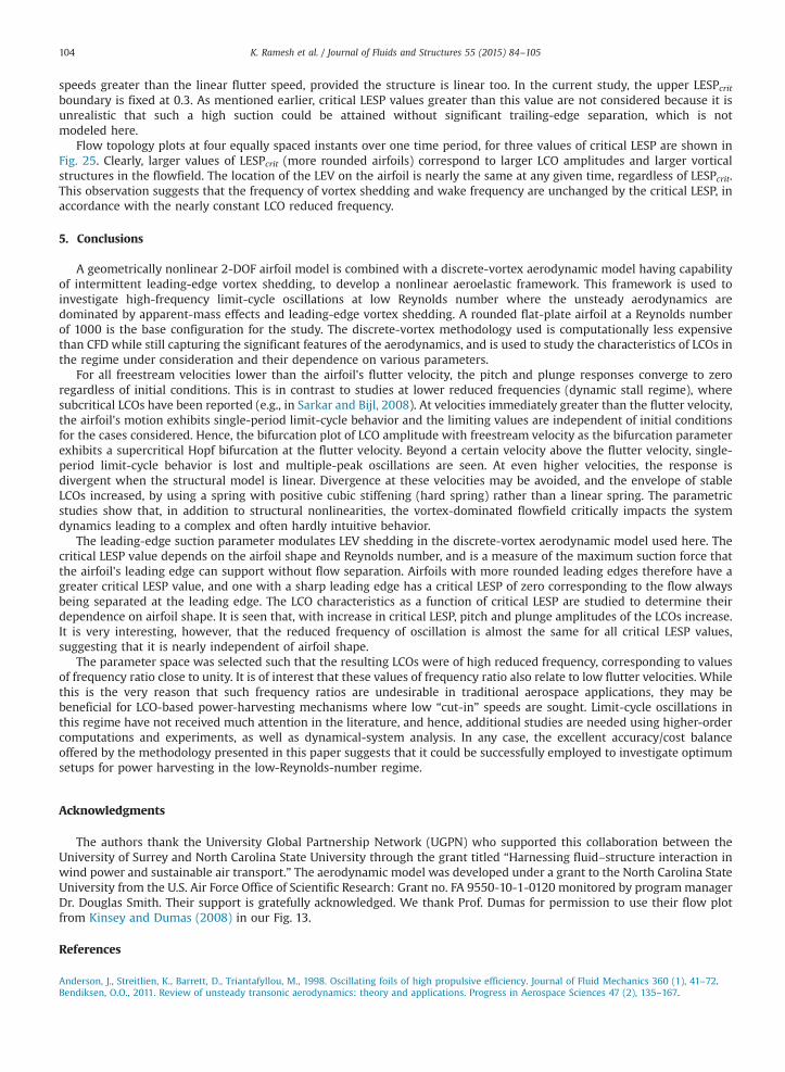
Fig. 23(a) and (b) shows the variation in pitch and plunge amplitudes of the resulting LCO over the parameter spaceidentified from Fig. 14. Three values of xα (0.05, 0.1, 0.2) and frequency ratios between 1.0 and 1.3 are considered. Thevariation of LCO amplitudes in this space is seen to be very nonlinear. This is likely because the static unbalance andfrequency ratio also affect the flutter speed, thereby making the relationship between the pitch/plunge amplitudes andthese parameters very complex. It is noted that some of the amplitudes are zero valued. These cases correspond tosimulations where the freestream velocity (Un ¼ 0:4667 from Table 1) is lower than the flutter velocity (which is a functionof xα and ω), thereby resulting in the response decaying to zero. Fig. 23(c) and (d) is plots of reduced frequency and phaseangle between pitch and plunge, for the LCOs in the chosen parameter space. The reduced frequency of response is seen tovary linearly with the frequency ratio (ω). Further, higher values of static unbalance (between 0.05 and 0.2), result in LCOs ofhigher frequency in pitch and plunge. It is noted again that this is the only study where the flutter velocity is also a functionof the varying parameters, thereby resulting in a complex and counter-intuitive variations of pitch- and plunge-LCOamplitudes.

Fig. 23. Parametric study C: LCO characteristics as function of structural parameters at a constant freestream velocity. The parameters listed in Table 1 areused as a baseline with xα and ω as variables: (a) pitch amplitude, (b) plunge amplitude, (c) reduced frequency, and (d) phase angle between pitch andplunge.

K. Ramesh et al. / Journal of Fluids and Structures 55 (2015) 84–105 103

4.6. Parametric study D: effect of change in airfoil shape (LESPcrit)

The critical value of leading edge suction parameter (LESP) governs leading-edge vortex shedding in the aerodynamicmodel. This value is independent of motion kinematics, but depends on the airfoil shape and Reynolds number of operation.Since different airfoil-Re combinations may result in various critical LESP values, it is of interest to study the variation in LCOcharacteristics as a function of critical LESP. The parameters in Table 1 are used as a baseline, with LESPcrit being a variable.

Limit-cycle properties (pitch and plunge amplitude, reduced frequency, and phase angle) are plotted against critical LESPin Fig. 24. As the value of LESPcrit increases, pitch and plunge amplitudes increase linearly. It is interesting, however, that thereduced frequency of response is nearly the same value and independent of critical LESP. In earlier research, Ramesh et al.(2012) have shown that airfoils with more rounded leading edges can support more suction, and hence have higher valuesof critical LESP. For example, a flat plate at Re¼1000 has LESPcrit ¼ 0:11, and a NACA0015 airfoil at the same Reynoldsnumber has LESPcrit ¼ 0:19. Hence, it follows that more rounded airfoils result in LCOs of greater amplitudes but the samefrequency. The increase in LCO amplitudes with critical LESP may be attributed to more a more rounded leading edge beingable to sustain more leading-edge suction, thereby bounding the LCOs at a larger amplitude.

It is noted that a zero value of critical LESP corresponds to a perfectly sharp leading edge with continuous vortexshedding from the leading edge, and a “very high” critical LESP value (LESPcrit ¼ 5) models no vortex shedding from theleading edge. Hence, in the case of the latter, the aerodynamic model is “linear” and destructive oscillations would occur at

Fig. 25. Parametric study D: flow topology plots for the limit-cycle responses obtained using different values of critical LESP. Plots (a)–(d) depict vorticitydistributions at four equally spaced time intervals over one period of the oscillation (a) tn/Tn=0; (b) tn/Tn=0.25; (c) tn/Tn=0.5; and (d) tn/Tn=0.75.

Fig. 24. Parametric study D: LCO characteristics as function of critical LESP value. The parameters listed in Table 1 are used as a baseline: (a) pitchamplitude, (b) plunge amplitude, (c) reduced frequency, and (d) phase angle between pitch and plunge.

K. Ramesh et al. / Journal of Fluids and Structures 55 (2015) 84–105104

speeds greater than the linear flutter speed, provided the structure is linear too. In the current study, the upper LESPcritboundary is fixed at 0.3. As mentioned earlier, critical LESP values greater than this value are not considered because it isunrealistic that such a high suction could be attained without significant trailing-edge separation, which is notmodeled here.

Flow topology plots at four equally spaced instants over one time period, for three values of critical LESP are shown inFig. 25. Clearly, larger values of LESPcrit (more rounded airfoils) correspond to larger LCO amplitudes and larger vorticalstructures in the flowfield. The location of the LEV on the airfoil is nearly the same at any given time, regardless of LESPcrit.This observation suggests that the frequency of vortex shedding and wake frequency are unchanged by the critical LESP, inaccordance with the nearly constant LCO reduced frequency.

5. Conclusions

A geometrically nonlinear 2-DOF airfoil model is combined with a discrete-vortex aerodynamic model having capabilityof intermittent leading-edge vortex shedding, to develop a nonlinear aeroelastic framework. This framework is used toinvestigate high-frequency limit-cycle oscillations at low Reynolds number where the unsteady aerodynamics aredominated by apparent-mass effects and leading-edge vortex shedding. A rounded flat-plate airfoil at a Reynolds numberof 1000 is the base configuration for the study. The discrete-vortex methodology used is computationally less expensivethan CFD while still capturing the significant features of the aerodynamics, and is used to study the characteristics of LCOs inthe regime under consideration and their dependence on various parameters.

For all freestream velocities lower than the airfoil's flutter velocity, the pitch and plunge responses converge to zeroregardless of initial conditions. This is in contrast to studies at lower reduced frequencies (dynamic stall regime), wheresubcritical LCOs have been reported (e.g., in Sarkar and Bijl, 2008). At velocities immediately greater than the flutter velocity,the airfoil's motion exhibits single-period limit-cycle behavior and the limiting values are independent of initial conditionsfor the cases considered. Hence, the bifurcation plot of LCO amplitude with freestream velocity as the bifurcation parameterexhibits a supercritical Hopf bifurcation at the flutter velocity. Beyond a certain velocity above the flutter velocity, single-period limit-cycle behavior is lost and multiple-peak oscillations are seen. At even higher velocities, the response isdivergent when the structural model is linear. Divergence at these velocities may be avoided, and the envelope of stableLCOs increased, by using a spring with positive cubic stiffening (hard spring) rather than a linear spring. The parametricstudies show that, in addition to structural nonlinearities, the vortex-dominated flowfield critically impacts the systemdynamics leading to a complex and often hardly intuitive behavior.

The leading-edge suction parameter modulates LEV shedding in the discrete-vortex aerodynamic model used here. Thecritical LESP value depends on the airfoil shape and Reynolds number, and is a measure of the maximum suction force thatthe airfoil's leading edge can support without flow separation. Airfoils with more rounded leading edges therefore have agreater critical LESP value, and one with a sharp leading edge has a critical LESP of zero corresponding to the flow alwaysbeing separated at the leading edge. The LCO characteristics as a function of critical LESP are studied to determine theirdependence on airfoil shape. It is seen that, with increase in critical LESP, pitch and plunge amplitudes of the LCOs increase.It is very interesting, however, that the reduced frequency of oscillation is almost the same for all critical LESP values,suggesting that it is nearly independent of airfoil shape.

The parameter space was selected such that the resulting LCOs were of high reduced frequency, corresponding to valuesof frequency ratio close to unity. It is of interest that these values of frequency ratio also relate to low flutter velocities. Whilethis is the very reason that such frequency ratios are undesirable in traditional aerospace applications, they may bebeneficial for LCO-based power-harvesting mechanisms where low “cut-in” speeds are sought. Limit-cycle oscillations inthis regime have not received much attention in the literature, and hence, additional studies are needed using higher-ordercomputations and experiments, as well as dynamical-system analysis. In any case, the excellent accuracy/cost balanceoffered by the methodology presented in this paper suggests that it could be successfully employed to investigate optimumsetups for power harvesting in the low-Reynolds-number regime.

Acknowledgments

The authors thank the University Global Partnership Network (UGPN) who supported this collaboration between theUniversity of Surrey and North Carolina State University through the grant titled “Harnessing fluid–structure interaction inwind power and sustainable air transport.” The aerodynamic model was developed under a grant to the North Carolina StateUniversity from the U.S. Air Force Office of Scientific Research: Grant no. FA 9550-10-1-0120 monitored by programmanagerDr. Douglas Smith. Their support is gratefully acknowledged. We thank Prof. Dumas for permission to use their flow plotfrom Kinsey and Dumas (2008) in our Fig. 13.

References

Anderson, J., Streitlien, K., Barrett, D., Triantafyllou, M., 1998. Oscillating foils of high propulsive efficiency. Journal of Fluid Mechanics 360 (1), 41–72.Bendiksen, O.O., 2011. Review of unsteady transonic aerodynamics: theory and applications. Progress in Aerospace Sciences 47 (2), 135–167.

K. Ramesh et al. / Journal of Fluids and Structures 55 (2015) 84–105 105

Bisplinghoff, R.L., Ashley, H., Halfman, R.L., 1996. Aeroelasticity. Courier Dover Publications, New York.Bryant, M., Garcia, E., 2011. Modeling and testing of a novel aeroelastic flutter energy harvester. Journal of Vibration and Acoustics 133 (1).Butcher, J.C., 2008. Numerical Methods for Ordinary Differential Equations, 2nd ed. John Wiley & Sons, Ltd, Chichester, UK.Carrier, J., Greengard, L., Rokhlin, V., 1988. A fast adaptive multipole algorithm for particle simulations. SIAM Journal on Scientific and Statistical Computing

9 (4), 669–686.Chantharasenawong, C., 2007. Nonlinear Aeroelastic Behaviour of Aerofoils Under Dynamic Stall (Ph.D. Thesis). Imperial College London, University of

London.Dickinson, M.H., Gotz, K.G., 1993. Unsteady aerodynamic performance of model wings at low Reynolds numbers. Journal of Experimental Biology 174 (1),

45–64.Dunnmon, J.A., Stanton, S.C., Mann, B.P., Dowell, E.H., 2011. Power extraction from aeroelastic limit cycle oscillations. Journal of Fluids and Structures 27 (8),

1182–1198.Ellington, C.P., 1999. The novel aerodynamics of insect flight: applications to micro-air vehicles. Journal of Experimental Biology 202 (23), 3439–3448.Ellington, C.P., vanden Berg, C., Willmott, A.P., Thomas, A.L.R., 1996. Leading-edge vortices in insect flight. Nature 384 (1), 626–630.FLUENT, Software Package, Ver. 6.1, ANSYS, Inc., Lebanon, NH, 2003.Fung, Y., 2002. An Introduction to the Theory of Aeroelasticity. Courier Dover Publications, New York.Garrick, I.E., 1937. Propulsion of a Flapping and Oscillating Airfoil. NACA Report 567.Hald, O.H., 1979. Convergence of vortex methods for Euler's equations, II. SIAM Journal on Numerical Analysis 16 (5), 726–755.Hamamoto, M., Ohta, Y., Hara, K., Hisada, T., 2007. Application of fluid–structure interaction analysis to flapping flight of insects with deformable wings.

Advanced Robotics 21 (1–2), 1–21.Jones, K.D., Platzer, M.F., 1996. Time-domain analysis of low-speed airfoil flutter. AIAA Journal 34 (5), 1027–1033.Kamakoti, R., Shyy, W., 2004. Fluid–structure interaction for aeroelastic applications. Progress in Aerospace Sciences 40 (8), 535–558.Katz, J., 1981. Discrete vortex method for the non-steady separated flow over an airfoil. Journal of Fluid Mechanics 102 (1), 315–328.Katz, J., Plotkin. A., 2000. Low-Speed Aerodynamics (Cambridge Aerospace Series).Kinsey, T., Dumas, G., 2008. Parametric study of an oscillating airfoil in a power-extraction regime. AIAA Journal 46 (6), 1318–1330.Kinsey, T., Dumas, G., Lalande, G., Ruel, J., Mehut, A., Viarouge, P., Lemay, J., Jean, Y., 2011. Prototype testing of a hydrokinetic turbine based on oscillating

hydrofoils. Renewable Energy 36 (6), 1710–1718.Lee, B.H.K., Price, S.J., Wong, Y.S., 1999a. Nonlinear aeroelastic analysis of airfoils: bifurcation and chaos. Progress in Aerospace Sciences 35 (3), 205–334.Lee, B.H.K., Jiang, L.Y., Wong, Y.S., 1999b. Flutter of an airfoil with a cubic restoring force. Journal of Fluids and Structures 13 (1), 75–101.Leishman, J.G., 2002. Principles of Helicopter Aerodynamics (Cambridge Aerospace Series).Leishman, J.G., Beddoes, T.S., 1989. A semi-empirical model for dynamic stall. Journal of the American Helicopter Society 34 (3), 3–17.Leonard, A., 1980. Vortex methods for flow simulation. Journal of Computational Physics 37 (3), 289–335.Liani, E., Guo, S., Allegri, G., 2007. Aeroelastic Effect on Flapping Wing Performance. AIAA Paper 2007-2412.Murua, J., Palacios, R., Peiró, J., 2010. Camber effects in the dynamic aeroelasticity of compliant airfoils. Journal of Fluids and Structures 26 (4), 527–543.Nakata, T., Liu, H., 2012. Aerodynamic performance of a hovering hawkmoth with flexible wings: a computational approach. Proceedings of the Royal

Society B: Biological Sciences 279 (1729), 722–731.Peng, Z., Zhu, Q., 2009. Energy harvesting through flow-induced oscillations of a foil. Physics of Fluids 21(123602).Poirel, D., Metivier, V., Dumas, G., 2011. Computational aeroelastic simulations of self-sustained pitch oscillations of a NACA0012 at transitional Reynolds

numbers. Journal of Fluids and Structures 27 (8), 1262–1277.Price, S.J., Alighanbari, H., Lee, B.H.K., 1995. The aeroelastic response of a two-dimensional airfoil with bilinear and cubic structural nonlinearities. Journal of

Fluids and Structures 9 (2), 175–193.Ramesh, K., Ke, J., Gopalarathnam, A., Edwards, J.R., 2012. Effect of Airfoil Shape and Reynolds Number on Leading Edge Vortex Shedding in Unsteady Flows.

AIAA Paper 2012–3025.Ramesh, K., Gopalarathnam, A., Edwards, J.R., Ol, M.V., Granlund, K., 2013. An unsteady airfoil theory applied to pitching motions validated against

experiment and computation. Theoretical and Computational Fluid Dynamics 27 (6), 843–864.Ramesh, K., Gopalarathnam, A., Granlund, K., Ol, M.V., Edwards, J.R., 2014. Discrete-vortex method with novel shedding criterion for unsteady airfoil flows

with intermittent leading-edge vortex shedding. Journal of Fluid Mechanics 751, 500–538.Sarkar, S., Bijl, H., 2008. Nonlinear aeroelastic behavior of an oscillating airfoil during stall-induced vibration. Journal of Fluids and Structures 24 (6),

757–777.Shyy, W., Liu, H., 2007. Flapping wings and aerodynamic lift: The role of leading-edge vortices. AIAA Journal 45(12).Shyy, W., Lian, Y., Tang, J., Liu, H., Trizila, P., Stanford, B., Bernal, L., Cesnik, C.E.S., Friedmann, P., Ifju, P., 2008. Computational aerodynamics of low Reynolds

number plunging pitching, and flexible wings for MAV applications. Acta Mechanica Sinica 24 (4), 351–373.Sváček, P., Feistauer, M., Horáček, J., 2007. Numerical simulation of flow induced airfoil vibrations with large amplitudes. Journal of Fluids and Structures 23

(3), 391–411.Tang, D.M., Dowell, E.H., 1993a. Comparison of theory and experiment for non-linear flutter and stall response of a helicopter blade. Journal of Sound and

Vibration 165 (2), 251–276.Tang, D.M., Dowell, E.H., 1993b. Nonlinear aeroelasticity in rotorcraft. Mathematical and Computer Modelling 18 (3), 157–184.Tang, J., Chimakurthi, S., Palacios, R., Cesnik, C.E.S., Shyy, W., 2008. Computational Fluid–Structure Interaction of a Deformable Flapping Wing for Micro Air

Vehicle Applications. AIAA Paper 2008-0615.Tang, L., Païdoussis, M.P., Jiang, J., 2009. Cantilevered flexible plates in axial flow: energy transfer and the concept of flutter-mill. Journal of Sound and

Vibration 326 (1), 263–276.Taylor, G.K., Triantafyllou, M.S., Tropea, C., 2010. Animal Locomotion. Springer-Verlag, Heidelberg.Theodorsen, T., 1935. General Theory of Aerodynamic Instability and the Mechanism of Flutter, NACA Report 496.Theodorsen, T., Garrick, I.E., 1942. Flutter Calculations in Three Degrees of Freedom, NACA Report 741.Tran, C.T., Petot, D., 1981. Semi-empirical model for the dynamic stall of airfoils in view of the application to the calculation of responses of a helicopter

blade in forward flight. Vertica 5, 35–53.Vatistas, G.H., Kozel, V., Mih, W.C., 1991. A simpler model for concentrated vortices. Experiments in Fluids 11 (1), 73–76.von Kármán, T., Burgers, J.M., 1935. General aerodynamic theory – perfect fluids. In: Durand, WF. (Ed.), Aerodynamic Theory: A General Review of Progress,

vol. 2. Dover Publications.Young, J., Lai, J., Platzer, M.F., 2014. A review of progress and challenges in flapping foil power generation. Progress in Aerospace Sciences 67, 2–28.