Journal of Financial Economics - docs.lhpedersen.comdocs.lhpedersen.com/BettingAgainstBeta.pdf ·...
25
Betting against beta $ Andrea Frazzini a , Lasse Heje Pedersen a,b,c,d,e,n a AQR Capital Management, CT 06830, USA b Stern School of Business, New York University, 44 West Fourth Street, Suite 9-190, NY 10012, USA c Copenhagen Business School, 2000 Frederiksberg, Denmark d Center for Economic Policy Research (CEPR), London, UK e National Bureau of Economic Research (NBER), MA, USA article info Article history: Received 16 December 2010 Received in revised form 10 April 2013 Accepted 19 April 2013 JEL classification: G01 G11 G12 G14 G15 Keywords: Asset prices Leverage constraints Margin requirements Liquidity Beta CAPM abstract We present a model with leverage and margin constraints that vary across investors and time. We find evidence consistent with each of the model's five central predictions: (1) Because constrained investors bid up high-beta assets, high beta is associated with low alpha, as we find empirically for US equities, 20 international equity markets, Treasury bonds, corporate bonds, and futures. (2) A betting against beta (BAB) factor, which is long leveraged low-beta assets and short high-beta assets, produces significant positive risk- adjusted returns. (3) When funding constraints tighten, the return of the BAB factor is low. (4) Increased funding liquidity risk compresses betas toward one. (5) More constrained investors hold riskier assets. & 2013 Elsevier B.V. All rights reserved. 1. Introduction A basic premise of the capital asset pricing model (CAPM) is that all agents invest in the portfolio with the highest expected excess return per unit of risk (Sharpe ratio) and leverage or de-leverage this portfolio to suit their risk preferences. However, many investors, such as individuals, pension funds, and mutual funds, are con- strained in the leverage that they can take, and they therefore overweight risky securities instead of using Contents lists available at ScienceDirect journal homepage: www.elsevier.com/locate/jfec Journal of Financial Economics 0304-405X/$ - see front matter & 2013 Elsevier B.V. All rights reserved. http://dx.doi.org/10.1016/j.jfineco.2013.10.005 ☆ We thank Cliff Asness, Aaron Brown, John Campbell, Josh Coval (discussant), Kent Daniel, Gene Fama, Nicolae Garleanu, John Heaton (discussant), Michael Katz, Owen Lamont, Juhani Linnainmaa (discussant), Michael Mendelson, Mark Mitchell, Lubos Pastor (discussant), Matt Richardson, William Schwert (editor), Tuomo Vuolteenaho, Robert Whitelaw and two anonymous referees for helpful comments and discussions as well as seminar participants at AQRCapital Management, Columbia University, New YorkUniversity, Yale University, Emory University, University of Chicago Booth School of Business, Northwestern University Kellogg School of Management, Harvard University, Boston University, Vienna University of Economics and Business, University of Mannheim, Goethe University Frankfurt, the American Finance Association meeting, NBER conference, Utah Winter Finance Conference, Annual Management Conference at University of Chicago Booth School of Business, Bank of America and Merrill Lynch Quant Conference, and Nomura Global Quantitative Investment Strategies Conference. Lasse Heje Pedersen gratefully acknowledges support from the European Research Council (ERC Grant no. 312417) and the FRIC Center for Financial Frictions (Grant no. DNRF102). n Corresponding author at: Stern School of Business, New York University, 44 West Fourth Street, Suite 9-190, NY 10012, USA. E-mail address: [email protected] (L.H. Pedersen). Journal of Financial Economics ] (]]]]) ]]]–]]] Please cite this article as: Frazzini, A., Pedersen, L.H., Betting against beta. Journal of Financial Economics (2013), http: //dx.doi.org/10.1016/j.jfineco.2013.10.005i
-
Upload
duongthuan -
Category
Documents
-
view
214 -
download
1
Transcript of Journal of Financial Economics - docs.lhpedersen.comdocs.lhpedersen.com/BettingAgainstBeta.pdf ·...

Contents lists available at ScienceDirect
Journal of Financial Economics
Journal of Financial Economics ] (]]]]) ]]]–]]]
0304-40http://d
☆ WeMichaelSchwerat AQRNorthwMannheManageQuantitno. 312
n CorrE-m
Pleas//dx.
journal homepage: www.elsevier.com/locate/jfec
Betting against beta$
Andrea Frazzini a, Lasse Heje Pedersen a,b,c,d,e,n
a AQR Capital Management, CT 06830, USAb Stern School of Business, New York University, 44 West Fourth Street, Suite 9-190, NY 10012, USAc Copenhagen Business School, 2000 Frederiksberg, Denmarkd Center for Economic Policy Research (CEPR), London, UKe National Bureau of Economic Research (NBER), MA, USA
a r t i c l e i n f o
Article history:Received 16 December 2010Received in revised form10 April 2013Accepted 19 April 2013
JEL classification:G01G11G12G14G15
Keywords:Asset pricesLeverage constraintsMargin requirementsLiquidityBetaCAPM
5X/$ - see front matter & 2013 Elsevier B.V.x.doi.org/10.1016/j.jfineco.2013.10.005
thank Cliff Asness, Aaron Brown, John CamKatz, Owen Lamont, Juhani Linnainmaa (d
t (editor), Tuomo Vuolteenaho, Robert WhitelCapital Management, Columbia University, Nestern University Kellogg School of Managemim, Goethe University Frankfurt, the Amement Conference at University of Chicago Bative Investment Strategies Conference. Lass417) and the FRIC Center for Financial Frictioesponding author at: Stern School of Busineail address: [email protected] (L.H. Ped
e cite this article as: Frazzini, A., Pdoi.org/10.1016/j.jfineco.2013.10.005
a b s t r a c t
We present a model with leverage and margin constraints that vary across investors andtime. We find evidence consistent with each of the model's five central predictions:(1) Because constrained investors bid up high-beta assets, high beta is associated with lowalpha, as we find empirically for US equities, 20 international equity markets, Treasurybonds, corporate bonds, and futures. (2) A betting against beta (BAB) factor, which is longleveraged low-beta assets and short high-beta assets, produces significant positive risk-adjusted returns. (3) When funding constraints tighten, the return of the BAB factor is low.(4) Increased funding liquidity risk compresses betas toward one. (5) More constrainedinvestors hold riskier assets.
& 2013 Elsevier B.V. All rights reserved.
1. Introduction
A basic premise of the capital asset pricing model(CAPM) is that all agents invest in the portfolio with thehighest expected excess return per unit of risk (Sharpe
All rights reserved.
pbell, Josh Coval (discussaniscussant), Michael Mendelsaw and two anonymous refeew York University, Yale Unient, Harvard University, Bosrican Finance Associationooth School of Business, Bae Heje Pedersen gratefullyns (Grant no. DNRF102).ss, New York University, 44ersen).
edersen, L.H., Betting ai
ratio) and leverage or de-leverage this portfolio to suittheir risk preferences. However, many investors, such asindividuals, pension funds, and mutual funds, are con-strained in the leverage that they can take, and theytherefore overweight risky securities instead of using
t), Kent Daniel, Gene Fama, Nicolae Garleanu, John Heaton (discussant),on, Mark Mitchell, Lubos Pastor (discussant), Matt Richardson, Williamrees for helpful comments and discussions as well as seminar participantsversity, Emory University, University of Chicago Booth School of Business,ton University, Vienna University of Economics and Business, University ofmeeting, NBER conference, Utah Winter Finance Conference, Annualnk of America and Merrill Lynch Quant Conference, and Nomura Globalacknowledges support from the European Research Council (ERC Grant
West Fourth Street, Suite 9-190, NY 10012, USA.
gainst beta. Journal of Financial Economics (2013), http:
A. Frazzini, L.H. Pedersen / Journal of Financial Economics ] (]]]]) ]]]–]]]2
leverage. For instance, many mutual fund families offerbalanced funds in which the “normal” fund may investaround 40% in long-term bonds and 60% in stocks, whereasthe “aggressive” fund invests 10% in bonds and 90% instocks. If the “normal” fund is efficient, then an investorcould leverage it and achieve a better trade-off betweenrisk and expected return than the aggressive portfolio witha large tilt toward stocks. The demand for exchange-tradedfunds (ETFs) with embedded leverage provides furtherevidence that many investors cannot use leverage directly.
This behavior of tilting toward high-beta assets sug-gests that risky high-beta assets require lower risk-adjusted returns than low-beta assets, which requireleverage. Indeed, the security market line for US stocks istoo flat relative to the CAPM (Black, Jensen, and Scholes,1972) and is better explained by the CAPM with restrictedborrowing than the standard CAPM [see Black (1972,1993), Brennan (1971), and Mehrling (2005) for an excel-lent historical perspective].
Several questions arise: How can an unconstrainedarbitrageur exploit this effect, i.e., how do you bet againstbeta? What is the magnitude of this anomaly relative tothe size, value, and momentum effects? Is betting againstbeta rewarded in other countries and asset classes? Howdoes the return premium vary over time and in the crosssection? Who bets against beta?
We address these questions by considering a dynamicmodel of leverage constraints and by presenting consistentempirical evidence from 20 international stock markets,Treasury bond markets, credit markets, and futuresmarkets.
Our model features several types of agents. Someagents cannot use leverage and, therefore, overweighthigh-beta assets, causing those assets to offer lowerreturns. Other agents can use leverage but face marginconstraints. Unconstrained agents underweight (or short-sell) high-beta assets and buy low-beta assets that theylever up. The model implies a flatter security market line(as in Black (1972)), where the slope depends on thetightness (i.e., Lagrange multiplier) of the funding con-straints on average across agents (Proposition 1).
One way to illustrate the asset pricing effect of thefunding friction is to consider the returns on market-neutral betting against beta (BAB) factors. A BAB factor isa portfolio that holds low-beta assets, leveraged to a betaof one, and that shorts high-beta assets, de-leveraged to abeta of one. For instance, the BAB factor for US stocksachieves a zero beta by holding $1.4 of low-beta stocks andshortselling $0.7 of high-beta stocks, with offsetting posi-tions in the risk-free asset to make it self-financing.1 Ourmodel predicts that BAB factors have a positive averagereturn and that the return is increasing in the ex antetightness of constraints and in the spread in betas betweenhigh- and low-beta securities (Proposition 2).
1 While we consider a variety of BAB factors within a number ofmarkets, one notable example is the zero-covariance portfolio introducedby Black (1972) and studied for US stocks by Black, Jensen, and Scholes(1972), Kandel (1984), Shanken (1985), Polk, Thompson, and Vuolteenaho(2006), and others.
Please cite this article as: Frazzini, A., Pedersen, L.H., Betting a//dx.doi.org/10.1016/j.jfineco.2013.10.005i
When the leveraged agents hit their margin constraint,they must de-leverage. Therefore, the model predicts that,during times of tightening funding liquidity constraints,the BAB factor realizes negative returns as its expectedfuture return rises (Proposition 3). Furthermore, the modelpredicts that the betas of securities in the cross section arecompressed toward one when funding liquidity risk is high(Proposition 4). Finally, the model implies that more-constrained investors overweight high-beta assets in theirportfolios and less-constrained investors overweight low-beta assets and possibly apply leverage (Proposition 5).
Our model thus extends the Black (1972) insight byconsidering a broader set of constraints and deriving thedynamic time series and cross-sectional properties arisingfrom the equilibrium interaction between agents withdifferent constraints.
We find consistent evidence for each of the model'scentral predictions. To test Proposition 1, we first considerportfolios sorted by beta within each asset class. We findthat alphas and Sharpe ratios are almost monotonicallydeclining in beta in each asset class. This finding providesbroad evidence that the relative flatness of the securitymarket line is not isolated to the US stock market but thatit is a pervasive global phenomenon. Hence, this pattern ofrequired returns is likely driven by a common economiccause, and our funding constraint model provides one suchunified explanation.
To test Proposition 2, we construct BAB factors withinthe US stock market and within each of the 19 otherdeveloped MSCI stock markets. The US BAB factor realizesa Sharpe ratio of 0.78 between 1926 and March 2012.To put this BAB factor return in perspective, note that itsSharpe ratio is about twice that of the value effect and 40%higher than that of momentum over the same time period.The BAB factor has highly significant risk-adjusted returns,accounting for its realized exposure to market, value, size,momentum, and liquidity factors (i.e., significant one-,three-, four-, and five-factor alphas), and it realizes asignificant positive return in each of the four 20-yearsubperiods between 1926 and 2012.
We find similar results in our sample of internationalequities. Combining stocks in each of the non-US countriesproduces a BAB factor with returns about as strong as theUS BAB factor.
We show that BAB returns are consistent across coun-tries, time, within deciles sorted by size, and within decilessorted by idiosyncratic risk and are robust to a number ofspecifications. These consistent results suggest that coin-cidence or data mining are unlikely explanations. How-ever, if leverage constraints are the underlying drivers as inour model, then the effect should also exist in othermarkets.
Hence, we examine BAB factors in other major assetclasses. For US Treasuries, the BAB factor is a portfolio thatholds leveraged low-beta (i.e., short-maturity) bonds andshortsells de-leveraged high-beta (i.e., long-term) bonds.This portfolio produces highly significant risk-adjustedreturns with a Sharpe ratio of 0.81. This profitability ofshortselling long-term bonds could seem to contradict thewell-known “term premium” in fixed income markets.There is no paradox, however. The term premium means
gainst beta. Journal of Financial Economics (2013), http:
2 This effect disappears when controlling for the maximum dailyreturn over the past month (Bali, Cakici, and Whitelaw, 2011) and whenusing other measures of idiosyncratic volatility (Fu, 2009).
3 The dividends and shares outstanding are taken as exogenous. Ourmodified CAPM has implications for a corporation's optimal capitalstructure, which suggests an interesting avenue of future researchbeyond the scope of this paper.
A. Frazzini, L.H. Pedersen / Journal of Financial Economics ] (]]]]) ]]]–]]] 3
that investors are compensated on average for holdinglong-term bonds instead of T-bills because of the need formaturity transformation. The term premium exists at allhorizons, however. Just as investors are compensated forholding ten-year bonds over T-bills, they are also compen-sated for holding one-year bonds. Our finding is that thecompensation per unit of risk is in fact larger for the one-year bond than for the ten-year bond. Hence, a portfoliothat has a leveraged long position in one-year (and othershort-term) bonds and a short position in long-term bondsproduces positive returns. This result is consistent withour model in which some investors are leverage-constrained in their bond exposure and, therefore, requirelower risk-adjusted returns for long-term bonds that givemore “bang for the buck”. Indeed, short-term bondsrequire tremendous leverage to achieve similar risk orreturn as long-term bonds. These results complementthose of Fama (1984, 1986) and Duffee (2010), who alsoconsider Sharpe ratios across maturities implied by stan-dard term structure models.
We find similar evidence in credit markets: A leveragedportfolio of highly rated corporate bonds outperforms ade-leveraged portfolio of low-rated bonds. Similarly, usinga BAB factor based on corporate bond indices by maturityproduces high risk-adjusted returns.
We test the time series predictions of Proposition 3using the TED spread as a measure of funding conditions.Consistent with the model, a higher TED spread is asso-ciated with low contemporaneous BAB returns. The laggedTED spread predicts returns negatively, which is incon-sistent with the model if a high TED spread means a hightightness of investors' funding constraints. This resultcould be explained if higher TED spreads meant thatinvestors' funding constraints would be tightening as theirbanks reduce credit availability over time, though this isspeculation.
To test the prediction of Proposition 4, we use thevolatility of the TED spread as an empirical proxy forfunding liquidity risk. Consistent with the model's beta-compression prediction, we find that the dispersion ofbetas is significantly lower when funding liquidity riskis high.
Lastly, we find evidence consistent with the model'sportfolio prediction that more-constrained investors holdhigher-beta securities than less-constrained investors(Proposition 5). We study the equity portfolios of mutualfunds and individual investors, which are likely to beconstrained. Consistent with the model, we find that theseinvestors hold portfolios with average betas above one.On the other side of the market, we find that leveragedbuyout (LBO) funds acquire firms with average betasbelow 1 and apply leverage. Similarly, looking at theholdings of Warren Buffett's firm Berkshire Hathaway,we see that Buffett bets against beta by buying low-betastocks and applying leverage (analyzed further in Frazzini,Kabiller, and Pedersen (2012)).
Our results shed new light on the relation between riskand expected returns. This central issue in financial eco-nomics has naturally received much attention. The stan-dard CAPM beta cannot explain the cross section ofunconditional stock returns (Fama and French, 1992) or
Please cite this article as: Frazzini, A., Pedersen, L.H., Betting a//dx.doi.org/10.1016/j.jfineco.2013.10.005i
conditional stock returns (Lewellen and Nagel, 2006).Stocks with high beta have been found to deliver lowrisk-adjusted returns (Black, Jensen, and Scholes, 1972;Baker, Bradley, and Wurgler, 2011); thus, the constrained-borrowing CAPM has a better fit (Gibbons, 1982; Kandel,1984; Shanken, 1985). Stocks with high idiosyncraticvolatility have realized low returns (Falkenstein, 1994;Ang, Hodrick, Xing, Zhang, 2006, 2009), but we find thatthe beta effect holds even when controlling for idiosyn-cratic risk.2 Theoretically, asset pricing models with bench-marked managers (Brennan, 1993) or constraints implymore general CAPM-like relations (Hindy, 1995; Cuoco,1997). In particular, the margin-CAPM implies that high-margin assets have higher required returns, especiallyduring times of funding illiquidity (Garleanu andPedersen, 2011; Ashcraft, Garleanu, and Pedersen, 2010).Garleanu and Pedersen (2011) show empirically thatdeviations of the law of one price arises when high-margin assets become cheaper than low-margin assets,and Ashcraft, Garleanu, and Pedersen (2010) find thatprices increase when central bank lending facilities reducemargins. Furthermore, funding liquidity risk is linked tomarket liquidity risk (Gromb and Vayanos, 2002;Brunnermeier and Pedersen, 2009), which also affectsrequired returns (Acharya and Pedersen, 2005). We com-plement the literature by deriving new cross-sectional andtime series predictions in a simple dynamic model thatcaptures leverage and margin constraints and by testing itsimplications across a broad cross section of securitiesacross all the major asset classes. Finally, Asness, Frazzini,and Pedersen (2012) report evidence of a low-beta effectacross asset classes consistent with our theory.
The rest of the paper is organized as follows. Section 2lays out the theory, Section 3 describes our data andempirical methodology, Sections 4–7 test Propositions 1–5,and Section 8 concludes. Appendix A contains all proofs,Appendix B provides a number of additional empiricalresults and robustness tests, and Appendix C provides acalibration of the model. The calibration shows that, tomatch the strong BAB performance in the data, a largefraction of agents must face severe constraints. An interest-ing topic for future research is to empirically estimateagents' leverage constraints and risk preferences and studywhether the magnitude of the BAB returns is consistentwith the model or should be viewed as a puzzle.
2. Theory
We consider an overlapping-generations (OLG) econ-omy in which agents i¼1,…,I are born each time period twith wealth Wi
t and live for two periods. Agents tradesecurities s¼1,…,S, where security s pays dividends δst andhas xns shares outstanding.3 Each time period t, young
gainst beta. Journal of Financial Economics (2013), http:
A. Frazzini, L.H. Pedersen / Journal of Financial Economics ] (]]]]) ]]]–]]]4
agents choose a portfolio of shares x¼(x1,…,xS)′, investingthe rest of their wealth at the risk-free return rf, tomaximize their utility:
max x′ðEtðPtþ1þδtþ1Þ�ð1þrf ÞPtÞ�γi
2x′Ωtx; ð1Þ
where Pt is the vector of prices at time t, Ωt is the variance–covariance matrix of Ptþ1þδtþ1, and γi is agent i's riskaversion. Agent i is subject to the portfolio constraint
mit∑sxsPs
trWit ð2Þ
This constraint requires that some multiple mit of the total
dollars invested, the sum of the number of shares xs timestheir prices Ps, must be less than the agent's wealth.
The investment constraint depends on the agent i. Forinstance, some agents simply cannot use leverage, which iscaptured by mi¼1 [as Black (1972) assumes]. Other agentsnot only could be precluded from using leverage but alsomust have some of their wealth in cash, which is capturedbymi greater than one. For instance, mi¼1/(1�0.20)¼1.25represents an agent who must hold 20% of her wealth incash. For instance, a mutual fund could need some readycash to be able to meet daily redemptions, an insurancecompany needs to pay claims, and individual investorsmay need cash for unforeseen expenses.
Other agents could be able to use leverage but couldface margin constraints. For instance, if an agent faces amargin requirement of 50%, then his mi is 0.50. With thismargin requirement, the agent can invest in assets worthtwice his wealth at most. A smaller margin requirement mi
naturally means that the agent can take greater positions.Our formulation assumes for simplicity that all securitieshave the same margin requirement, which may be truewhen comparing securities within the same asset class(e.g., stocks), as we do empirically. Garleanu and Pedersen(2011) and Ashcraft, Garleanu, and Pedersen (2010) con-sider assets with different margin requirements and showtheoretically and empirically that higher margin require-ments are associated with higher required returns(Margin CAPM).
We are interested in the properties of the competitiveequilibrium in which the total demand equals the supply:
∑ixi ¼ xn ð3Þ
To derive equilibrium, consider the first order condition foragent i:
0¼ EtðPtþ1þδtþ1Þ�ð1þrf ÞPt�γiΩxi�ψ itPt ; ð4Þ
where ψi is the Lagrange multiplier of the portfolio con-straint. Solving for xi gives the optimal position:
xi ¼ 1γiΩ�1ðEtðPtþ1þδtþ1Þ�ð1þrf þψ i
tÞPtÞ: ð5Þ
The equilibrium condition now follows from summingover these positions:
xn ¼ 1γΩ�1ðEtðPtþ1þδtþ1Þ�ð1þrf þψ tÞPtÞ; ð6Þ
where the aggregate risk aversion γ is defined by 1/γ¼Σi1/γi and ψ t ¼∑iðγ=γiÞψ i
t is the weighted average Lagrange
Please cite this article as: Frazzini, A., Pedersen, L.H., Betting a//dx.doi.org/10.1016/j.jfineco.2013.10.005i
multiplier. (The coefficients γ/γi sum to one by definition ofthe aggregate risk aversion γ.) The equilibrium price canthen be computed:
Pt ¼ EtðPtþ1þδtþ1Þ�γΩxn
1þrf þψ t; ð7Þ
Translating this into the return of any security ritþ1 ¼ðPi
tþ1þδitþ1Þ=Pit�1, the return on the market rMtþ1,
and using the usual expression for beta, βst ¼ covtðrstþ1; r
Mtþ1Þ=vartðrMtþ1Þ, we obtain the following results.
(All proofs are in Appendix A, which also illustrates theportfolio choice with leverage constraints in a mean-standard deviation diagram.)
Proposition 1 (high beta is low alpha).
(i)
gain
The equilibrium required return for any security s is
Etðrstþ1Þ ¼ rf þψ tþβstλt ð8Þwhere the risk premium is λt ¼ EtðrMtþ1Þ�rf �ψ t and ψtis the average Lagrange multiplier, measuring the tight-ness of funding constraints.
(ii)
A security's alpha with respect to the market isαst ¼ ψ tð1�βst Þ. The alpha decreases in the beta, βst .(iii)
For an efficient portfolio, the Sharpe ratio is highest foran efficient portfolio with a beta less than one anddecreases in βst for higher betas and increases for lowerbetas.As in Black's CAPM with restricted borrowing (in whichmi¼1 for all agents), the required return is a constant plusbeta times a risk premium. Our expression shows expli-citly how risk premia are affected by the tightness ofagents' portfolio constraints, as measured by the averageLagrange multiplier ψt. Tighter portfolio constraints (i.e., alarger ψt) flatten the security market line by increasing theintercept and decreasing the slope λt.Whereas the standard CAPM implies that the intercept
of the security market line is rf, the intercept here isincreased by binding funding constraints (through theweighted average of the agents' Lagrange multipliers).One could wonder why zero-beta assets require returnsin excess of the risk-free rate. The answer has two parts.First, constrained agents prefer to invest their limitedcapital in riskier assets with higher expected return.Second, unconstrained agents do invest considerableamounts in zero-beta assets so, from their perspective,the risk of these assets is not idiosyncratic, as additionalexposure to such assets would increase the risk of theirportfolio. Hence, in equilibrium, zero-beta risky assetsmust offer higher returns than the risk-free rate.Assets that have zero covariance to the Tobin (1958)
“tangency portfolio” held by an unconstrained agent doearn the risk-free rate, but the tangency portfolio is not themarket portfolio in our equilibrium. The market portfoliois the weighted average of all investors' portfolios, i.e., anaverage of the tangency portfolio held by unconstrainedinvestors and riskier portfolios held by constrained inves-tors. Hence, the market portfolio has higher risk andexpected return than the tangency portfolio, but a lowerSharpe ratio.
st beta. Journal of Financial Economics (2013), http:
A. Frazzini, L.H. Pedersen / Journal of Financial Economics ] (]]]]) ]]]–]]] 5
The portfolio constraints further imply a lower slope λtof the security market line, i.e., a lower compensation for amarginal increase in systematic risk. The slope is lowerbecause constrained agents need high unleveraged returnsand are, therefore, willing to accept less compensation forhigher risk.4
We next consider the properties of a factor that goeslong low-beta assets and shortsells high-beta assets.To construct such a factor, let wL be the relative portfolioweights for a portfolio of low-beta assets with returnrLtþ1 ¼w′
Lrtþ1 and consider similarly a portfolio of high-beta assets with return rHtþ1. The betas of these portfoliosare denoted βLt and βHt , where βLt oβHt . We then construct abetting against beta (BAB) factor as
rBABtþ1 ¼1βLt
ðrLtþ1�rf Þ� 1βHt
ðrHtþ1�rf Þ ð9Þ
this portfolio is market-neutral; that is, it has a beta ofzero. The long side has been leveraged to a beta of one, andthe short side has been de-leveraged to a beta of one.Furthermore, the BAB factor provides the excess return ona self-financing portfolio, such as HML (high minus low)and SMB (small minus big), because it is a differencebetween excess returns. The difference is that BAB is notdollar-neutral in terms of only the risky securities becausethis would not produce a beta of zero.5 The model hasseveral predictions regarding the BAB factor.
Proposition 2 (positive expected return of BAB). The expectedexcess return of the self-financing BAB factor is positive
EtðrBABtþ1Þ ¼βHt �βLtβLtβ
Ht
ψ tZ0 ð10Þ
and increasing in the ex ante beta spread ðβHt �βLt Þ=ðβLtβHt Þ andfunding tightness ψt.
Proposition 2 shows that a market-neutral BAB portfoliothat is long leveraged low-beta securities and short higher-beta securities earns a positive expected return on average.The size of the expected return depends on the spread inthe betas and how binding the portfolio constraints are inthe market, as captured by the average of the Lagrangemultipliers ψt.Proposition 3 considers the effect of a shock to the
portfolio constraints (or margin requirements), mk, whichcan be interpreted as a worsening of funding liquidity,
4 While the risk premium implied by our theory is lower than theone implied by the CAPM, it is still positive. It is difficult to empiricallyestimate a low risk premium and its positivity is not a focus of ourempirical tests as it does not distinguish our theory from the standardCAPM. However, the data are generally not inconsistent with ourprediction as the estimated risk premium is positive and insignificantfor US stocks, negative and insignificant for international stocks, positiveand insignificant for Treasuries, positive and significant for credits acrossmaturities, and positive and significant across asset classes.
5 A natural BAB factor is the zero-covariance portfolio of Black (1972)and Black, Jensen, and Scholes (1972). We consider a broader class of BABportfolios because we empirically consider a variety of BAB portfolioswithin various asset classes that are subsets of all securities (e.g., stocks ina particular size group). Therefore, our construction achieves marketneutrality by leveraging (and de-leveraging) the long and short sidesinstead of adding the market itself as Black, Jensen, and Scholes(1972) do.
Please cite this article as: Frazzini, A., Pedersen, L.H., Betting a//dx.doi.org/10.1016/j.jfineco.2013.10.005i
a credit crisis in the extreme. Such a funding liquidityshock results in losses for the BAB factor as its requiredreturn increases. This happens because agents may need tode-leverage their bets against beta or stretch even furtherto buy the high-beta assets. Thus, the BAB factor isexposed to funding liquidity risk, as it loses when portfolioconstraints become more binding.
Proposition 3 (funding shocks and BAB returns). A tighterportfolio constraint, that is, an increase in mk
t for some of k,leads to a contemporaneous loss for the BAB factor
∂rBABt
∂mkt
r0 ð11Þ
and an increase in its future required return:
∂EtðrBABtþ1Þ∂mk
t
Z0 ð12Þ
Funding shocks have further implications for the crosssection of asset returns and the BAB portfolio. Specifically,a funding shock makes all security prices drop together(that is, ð∂Ps
t=∂ψ tÞ=Pst is the same for all securities s).
Therefore, an increased funding risk compresses betastoward one.6 If the BAB portfolio construction is basedon an information set that does not account for thisincreased funding risk, then the BAB portfolio's conditionalmarket beta is affected.
Proposition 4 (beta compression). Suppose that all randomvariables are identically and independently distributed (i.i.d.)over time and δt is independent of the other randomvariables. Further, at time t�1 after the BAB portfolio isformed and prices are set, the conditional variance of thediscount factor 1/(1þrfþψt) rises (falls) due to new informa-tion about mt and Wt. Then,
(i)
6
ingrequhaverisesmakdiffecasetowa
gain
The conditional return betas βit�1 of all securities arecompressed toward one (more dispersed), and
(ii)
The conditional beta of the BAB portfolio becomespositive (negative), even though it is market neutralrelative to the information set used for portfolioformation.In addition to the asset-pricing predictions that wederive, funding constraints naturally affect agents' portfo-lio choices. In particular, more-constrained investors tilttoward riskier securities in equilibrium and less-constrained agents tilt toward safer securities with higherreward per unit of risk. To state this result, we write next
Garleanu and Pedersen (2011) find a complementary result, study-securities with identical fundamental risk but different marginirements. They find theoretically and empirically that such assetssimilar betas when liquidity is good, but when funding liquidity riskthe high-margin securities have larger betas, as their high marginse them more funding sensitive. Here, we study securities withrent fundamental risk, but the same margin requirements. In this, higher funding liquidity risk means that betas are compressedrd one.
st beta. Journal of Financial Economics (2013), http:
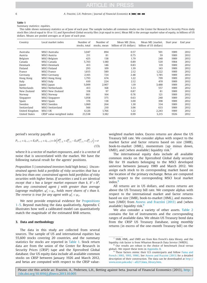
Table 1Summary statistics: equities.
This table shows summary statistics as of June of each year. The sample includes all commons stocks on the Center for Research in Security Prices dailystock files (shrcd equal to 10 or 11) and Xpressfeed Global security files (tcpi equal to zero). Mean ME is the average market value of equity, in billions of USdollars. Means are pooled averages as of June of each year.
Country Local market index Number ofstocks, total
Number ofstocks, mean
Mean ME (firm,billion of US dollars)
Mean ME (market,billion of US dollars)
Start year End year
Australia MSCI Australia 3,047 894 0.57 501 1989 2012Austria MSCI Austria 211 81 0.75 59 1989 2012Belgium MSCI Belgium 425 138 1.79 240 1989 2012Canada MSCI Canada 5,703 1,180 0.89 520 1984 2012Denmark MSCI Denmark 413 146 0.83 119 1989 2012Finland MSCI Finland 293 109 1.39 143 1989 2012France MSCI France 1,815 589 2.12 1,222 1989 2012Germany MSCI Germany 2,165 724 2.48 1,785 1989 2012Hong Kong MSCI Hong Kong 1,793 674 1.22 799 1989 2012Italy MSCI Italy 610 224 2.12 470 1989 2012Japan MSCI Japan 5,009 2,907 1.19 3,488 1989 2012Netherlands MSCI Netherlands 413 168 3.33 557 1989 2012New Zealand MSCI New Zealand 318 97 0.87 81 1989 2012Norway MSCI Norway 661 164 0.76 121 1989 2012Singapore MSCI Singapore 1,058 375 0.63 240 1989 2012Spain MSCI Spain 376 138 3.00 398 1989 2012Sweden MSCI Sweden 1,060 264 1.30 334 1989 2012Switzerland MSCI Switzerland 566 210 3.06 633 1989 2012United Kingdom MSCI UK 6,126 1,766 1.22 2,243 1989 2012United States CRSP value-weighted index 23,538 3,182 0.99 3,215 1926 2012
7 SMB, HML, and UMD are from Ken French's data library, and theliquidity risk factor is from Wharton Research Data Service (WRDS).
8 Our results are robust to the choice of benchmark (local versusglobal). We report these tests in Appendix B.
9 These factors mimic their U.S counterparts and follow Fama andFrench (1992, 1993, 1996). See Asness and Frazzini (2013) for a detaileddescription of their construction. The data can be downloaded at http://www.econ.yale.edu/�af227/data_library.htm.
A. Frazzini, L.H. Pedersen / Journal of Financial Economics ] (]]]]) ]]]–]]]6
period's security payoffs as
Ptþ1þδtþ1 ¼ EtðPtþ1þδtþ1Þþb PMtþ1þδMtþ1�EtðPM
tþ1þδMtþ1Þ� �
þe
ð13Þwhere b is a vector of market exposures, and e is a vector ofnoise that is uncorrelated with the market. We have thefollowing natural result for the agents' positions.
Proposition 5 (constrained investors hold high betas). Uncon-strained agents hold a portfolio of risky securities that has abeta less than one; constrained agents hold portfolios of riskysecurities with higher betas. If securities s and k are identicalexcept that s has a larger market exposure than k, bs4bk,then any constrained agent j with greater than averageLagrange multiplier, ψ j
t4ψ t , holds more shares of s than k.The reverse is true for any agent with ψ j
toψ t .
We next provide empirical evidence for Propositions1–5. Beyond matching the data qualitatively, Appendix Cillustrates how well a calibrated model can quantitativelymatch the magnitude of the estimated BAB returns.
3. Data and methodology
The data in this study are collected from severalsources. The sample of US and international equities has55,600 stocks covering 20 countries, and the summarystatistics for stocks are reported in Table 1. Stock returndata are from the union of the Center for Research inSecurity Prices (CRSP) tape and the Xpressfeed Globaldatabase. Our US equity data include all available commonstocks on CRSP between January 1926 and March 2012,and betas are computed with respect to the CRSP value-
Please cite this article as: Frazzini, A., Pedersen, L.H., Betting a//dx.doi.org/10.1016/j.jfineco.2013.10.005i
weighted market index. Excess returns are above the USTreasury bill rate. We consider alphas with respect to themarket factor and factor returns based on size (SMB),book-to-market (HML), momentum (up minus down,UMD), and (when available) liquidity risk.7
The international equity data include all availablecommon stocks on the Xpressfeed Global daily securityfile for 19 markets belonging to the MSCI developeduniverse between January 1989 and March 2012. Weassign each stock to its corresponding market based onthe location of the primary exchange. Betas are computedwith respect to the corresponding MSCI local marketindex.8
All returns are in US dollars, and excess returns areabove the US Treasury bill rate. We compute alphas withrespect to the international market and factor returnsbased on size (SMB), book-to-market (HML), and momen-tum (UMD) from Asness and Frazzini (2013) and (whenavailable) liquidity risk.9
We also consider a variety of other assets. Table 2contains the list of instruments and the correspondingranges of available data. We obtain US Treasury bond datafrom the CRSP US Treasury Database, using monthlyreturns (in excess of the one-month Treasury bill) on the
gainst beta. Journal of Financial Economics (2013), http:
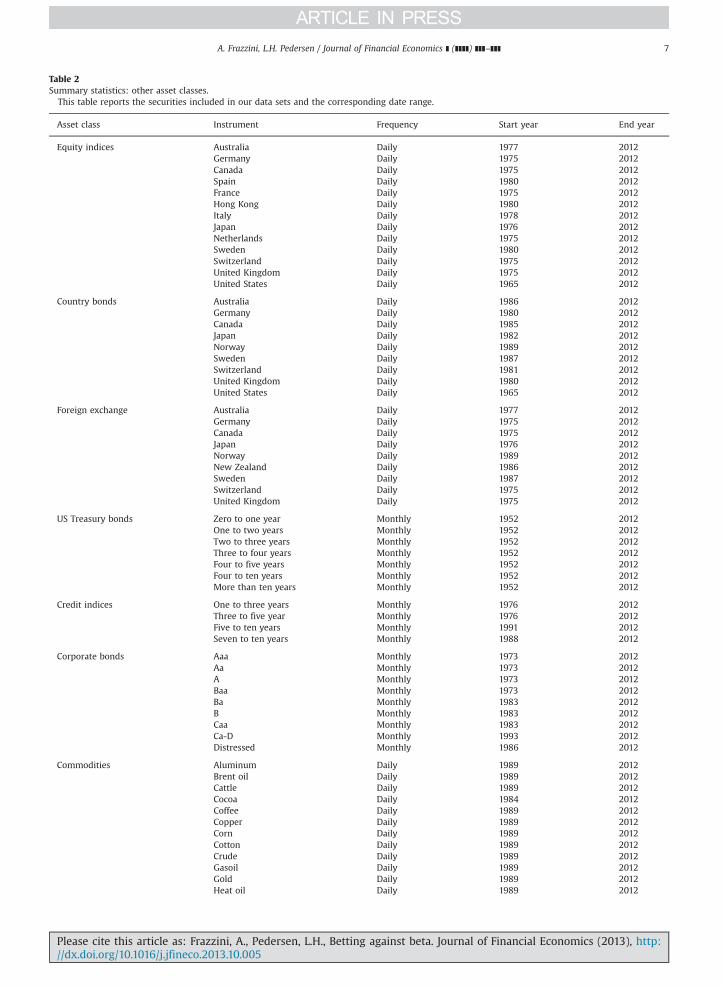
Table 2Summary statistics: other asset classes.
This table reports the securities included in our data sets and the corresponding date range.
Asset class Instrument Frequency Start year End year
Equity indices Australia Daily 1977 2012Germany Daily 1975 2012Canada Daily 1975 2012Spain Daily 1980 2012France Daily 1975 2012Hong Kong Daily 1980 2012Italy Daily 1978 2012Japan Daily 1976 2012Netherlands Daily 1975 2012Sweden Daily 1980 2012Switzerland Daily 1975 2012United Kingdom Daily 1975 2012United States Daily 1965 2012
Country bonds Australia Daily 1986 2012Germany Daily 1980 2012Canada Daily 1985 2012Japan Daily 1982 2012Norway Daily 1989 2012Sweden Daily 1987 2012Switzerland Daily 1981 2012United Kingdom Daily 1980 2012United States Daily 1965 2012
Foreign exchange Australia Daily 1977 2012Germany Daily 1975 2012Canada Daily 1975 2012Japan Daily 1976 2012Norway Daily 1989 2012New Zealand Daily 1986 2012Sweden Daily 1987 2012Switzerland Daily 1975 2012United Kingdom Daily 1975 2012
US Treasury bonds Zero to one year Monthly 1952 2012One to two years Monthly 1952 2012Two to three years Monthly 1952 2012Three to four years Monthly 1952 2012Four to five years Monthly 1952 2012Four to ten years Monthly 1952 2012More than ten years Monthly 1952 2012
Credit indices One to three years Monthly 1976 2012Three to five year Monthly 1976 2012Five to ten years Monthly 1991 2012Seven to ten years Monthly 1988 2012
Corporate bonds Aaa Monthly 1973 2012Aa Monthly 1973 2012A Monthly 1973 2012Baa Monthly 1973 2012Ba Monthly 1983 2012B Monthly 1983 2012Caa Monthly 1983 2012Ca-D Monthly 1993 2012Distressed Monthly 1986 2012
Commodities Aluminum Daily 1989 2012Brent oil Daily 1989 2012Cattle Daily 1989 2012Cocoa Daily 1984 2012Coffee Daily 1989 2012Copper Daily 1989 2012Corn Daily 1989 2012Cotton Daily 1989 2012Crude Daily 1989 2012Gasoil Daily 1989 2012Gold Daily 1989 2012Heat oil Daily 1989 2012
Please cite this article as: Frazzini, A., Pedersen, L.H., Betting against beta. Journal of Financial Economics (2013), http://dx.doi.org/10.1016/j.jfineco.2013.10.005i
A. Frazzini, L.H. Pedersen / Journal of Financial Economics ] (]]]]) ]]]–]]] 7
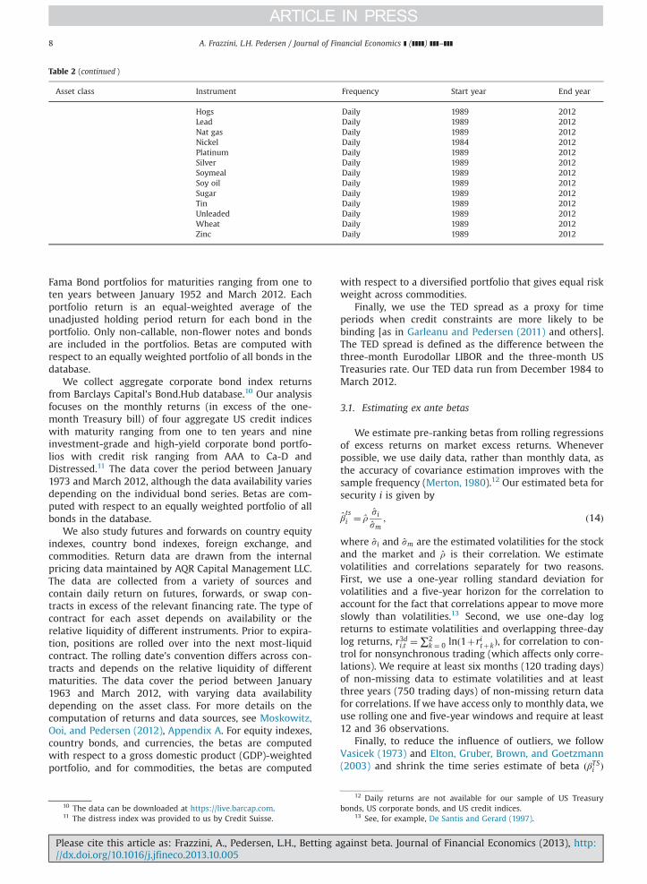
Table 2 (continued )
Asset class Instrument Frequency Start year End year
Hogs Daily 1989 2012Lead Daily 1989 2012Nat gas Daily 1989 2012Nickel Daily 1984 2012Platinum Daily 1989 2012Silver Daily 1989 2012Soymeal Daily 1989 2012Soy oil Daily 1989 2012Sugar Daily 1989 2012Tin Daily 1989 2012Unleaded Daily 1989 2012Wheat Daily 1989 2012Zinc Daily 1989 2012
A. Frazzini, L.H. Pedersen / Journal of Financial Economics ] (]]]]) ]]]–]]]8
Fama Bond portfolios for maturities ranging from one toten years between January 1952 and March 2012. Eachportfolio return is an equal-weighted average of theunadjusted holding period return for each bond in theportfolio. Only non-callable, non-flower notes and bondsare included in the portfolios. Betas are computed withrespect to an equally weighted portfolio of all bonds in thedatabase.
We collect aggregate corporate bond index returnsfrom Barclays Capital's Bond.Hub database.10 Our analysisfocuses on the monthly returns (in excess of the one-month Treasury bill) of four aggregate US credit indiceswith maturity ranging from one to ten years and nineinvestment-grade and high-yield corporate bond portfo-lios with credit risk ranging from AAA to Ca-D andDistressed.11 The data cover the period between January1973 and March 2012, although the data availability variesdepending on the individual bond series. Betas are com-puted with respect to an equally weighted portfolio of allbonds in the database.
We also study futures and forwards on country equityindexes, country bond indexes, foreign exchange, andcommodities. Return data are drawn from the internalpricing data maintained by AQR Capital Management LLC.The data are collected from a variety of sources andcontain daily return on futures, forwards, or swap con-tracts in excess of the relevant financing rate. The type ofcontract for each asset depends on availability or therelative liquidity of different instruments. Prior to expira-tion, positions are rolled over into the next most-liquidcontract. The rolling date's convention differs across con-tracts and depends on the relative liquidity of differentmaturities. The data cover the period between January1963 and March 2012, with varying data availabilitydepending on the asset class. For more details on thecomputation of returns and data sources, see Moskowitz,Ooi, and Pedersen (2012), Appendix A. For equity indexes,country bonds, and currencies, the betas are computedwith respect to a gross domestic product (GDP)-weightedportfolio, and for commodities, the betas are computed
10 The data can be downloaded at https://live.barcap.com.11 The distress index was provided to us by Credit Suisse.
Please cite this article as: Frazzini, A., Pedersen, L.H., Betting a//dx.doi.org/10.1016/j.jfineco.2013.10.005i
with respect to a diversified portfolio that gives equal riskweight across commodities.
Finally, we use the TED spread as a proxy for timeperiods when credit constraints are more likely to bebinding [as in Garleanu and Pedersen (2011) and others].The TED spread is defined as the difference between thethree-month Eurodollar LIBOR and the three-month USTreasuries rate. Our TED data run from December 1984 toMarch 2012.
3.1. Estimating ex ante betas
We estimate pre-ranking betas from rolling regressionsof excess returns on market excess returns. Wheneverpossible, we use daily data, rather than monthly data, asthe accuracy of covariance estimation improves with thesample frequency (Merton, 1980).12 Our estimated beta forsecurity i is given by
βtsi ¼ ρ
sism
; ð14Þ
where si and sm are the estimated volatilities for the stockand the market and ρ is their correlation. We estimatevolatilities and correlations separately for two reasons.First, we use a one-year rolling standard deviation forvolatilities and a five-year horizon for the correlation toaccount for the fact that correlations appear to move moreslowly than volatilities.13 Second, we use one-day logreturns to estimate volatilities and overlapping three-daylog returns, r3di;t ¼∑2
k ¼ 0 lnð1þritþkÞ, for correlation to con-trol for nonsynchronous trading (which affects only corre-lations). We require at least six months (120 trading days)of non-missing data to estimate volatilities and at leastthree years (750 trading days) of non-missing return datafor correlations. If we have access only to monthly data, weuse rolling one and five-year windows and require at least12 and 36 observations.
Finally, to reduce the influence of outliers, we followVasicek (1973) and Elton, Gruber, Brown, and Goetzmann(2003) and shrink the time series estimate of beta ðβTSi Þ
12 Daily returns are not available for our sample of US Treasurybonds, US corporate bonds, and US credit indices.
13 See, for example, De Santis and Gerard (1997).
gainst beta. Journal of Financial Economics (2013), http:
A. Frazzini, L.H. Pedersen / Journal of Financial Economics ] (]]]]) ]]]–]]] 9
toward the cross-sectional mean ðβXSÞ:
βi ¼wiβTSi þð1�wiÞβ
XS ð15Þ
for simplicity, instead of having asset-specific and time-varying shrinkage factors as in Vasicek (1973), we setw¼0.6 and βXS¼1 for all periods and across all assets.However, our results are very similar either way.14
Our choice of the shrinkage factor does not affect howsecurities are sorted into portfolios because the commonshrinkage does not change the ranks of the security betas.However, the amount of shrinkage affects the construction ofthe BAB portfolios because the estimated betas are used toscale the long and short sides of portfolio as seen in Eq. (9).
To account for the fact that noise in the ex ante betasaffects the construction of the BAB factors, our inference isfocused on realized abnormal returns so that any mis-match between ex ante and (ex post) realized betas ispicked up by the realized loadings in the factor regression.When we regress our portfolios on standard risk factors,the realized factor loadings are not shrunk as abovebecause only the ex ante betas are subject to selectionbias. Our results are robust to alternative beta estimationprocedures as we report in Appendix B.
We compute betas with respect to a market portfolio,which is either specific to an asset class or the overallworld market portfolio of all assets. While our results holdboth ways, we focus on betas with respect to asset class-specific market portfolios because these betas are lessnoisy for several reasons. First, this approach allows us touse daily data over a long time period for most assetclasses, as opposed to using the most diversified marketportfolio for which we only have monthly data and onlyover a limited time period. Second, this approach isapplicable even if markets are segmented.
As a robustness test, Table B8 in Appendix B reportsresults when we compute betas with respect to a proxy for aworld market portfolio consisting of many asset classes. Weuse the world market portfolio from Asness, Frazzini, andPedersen (2012).15 The results are consistent with our maintests as the BAB factors earn large and significant abnormalreturns in each of the asset classes in our sample.
3.2. Constructing betting against beta factors
We construct simple portfolios that are long low-betasecurities and that shortsell high-beta securities (BAB factors).To construct each BAB factor, all securities in an asset class areranked in ascending order on the basis of their estimatedbeta. The ranked securities are assigned to one of twoportfolios: low-beta and high-beta. The low- (high-) beta
14 The Vasicek (1973) Bayesian shrinkage factor is given bywi ¼ 1�s2i;TS=ðs2i;TSþs2XSÞ where s2i;TS is the variance of the estimated betafor security i and s2XS is the cross-sectional variance of betas. Thisestimator places more weight on the historical times series estimatewhen the estimate has a lower variance or when there is large dispersionof betas in the cross section. Pooling across all stocks in our US equitydata, the shrinkage factor w has a mean of 0.61.
15 See Asness, Frazzini, and Pedersen (2012) for a detailed descriptionof this market portfolio. The market series is monthly and ranges from1973 to 2009.
Please cite this article as: Frazzini, A., Pedersen, L.H., Betting a//dx.doi.org/10.1016/j.jfineco.2013.10.005i
portfolio is composed of all stocks with a beta below (above)its asset class median (or country median for internationalequities). In each portfolio, securities are weighted by theranked betas (i.e., lower-beta securities have larger weights inthe low-beta portfolio and higher-beta securities have largerweights in the high-beta portfolio). The portfolios are reba-lanced every calendar month.
More formally, let z be the n�1 vector of beta rankszi¼rank(βit) at portfolio formation, and let z¼ 1′
nz=n be theaverage rank, where n is the number of securities and 1n isan n�1 vector of ones. The portfolio weights of the low-beta and high-beta portfolios are given by
wH ¼ kðz�zÞþwL ¼ kðz�zÞ� ð16Þ
where k is a normalizing constant k¼ 2=1′njz�zj and xþ
and x� indicate the positive and negative elements of avector x. By construction, we have 1′
nwH ¼ 1 and 1′nwL ¼ 1.
To construct the BAB factor, both portfolios are rescaled tohave a beta of one at portfolio formation. The BAB is theself-financing zero-beta portfolio (8) that is long the low-beta portfolio and that shortsells the high-beta portfolio.
rBABtþ1 ¼1βLt
ðrLtþ1�rf Þ� 1βHt
ðrHtþ1�rf Þ; ð17Þ
where rLtþ1 ¼ r′tþ1wL; rHtþ1 ¼ r′tþ1 wH ; βLt ¼ β′twL; and βHt ¼ β′twH .
For example, on average, the US stock BAB factor is long$1.4 of low-beta stocks (financed by shortselling $1.4 ofrisk-free securities) and shortsells $0.7 of high-beta stocks(with $0.7 earning the risk-free rate).
3.3. Data used to test the theory's portfolio predictions
We collect mutual fund holdings from the union of theCRSP Mutual Fund Database and Thomson Financial CDA/Spectrum holdings database, which includes all registereddomestic mutual funds filing with the Securities and ExchangeCommission. The holdings data run from March 1980 toMarch 2012. We focus our analysis on open-end, activelymanaged, domestic equity mutual funds. Our sample selectionprocedure follows that of Kacperczyk, Sialm, and Zheng(2008), and we refer to their Appendix for details about thescreens that were used and summary statistics of the data.
Our individual investors' holdings data are collectedfrom a nationwide discount brokerage house and containtrades made by about 78 thousand households in theperiod from January 1991 to November 1996. This dataset has been used extensively in the existing literature onindividual investors. For a detailed description of thebrokerage data set, see Barber and Odean (2000).
Our sample of buyouts is drawn from the mergers andacquisitions and corporate events database maintained byAQR/CNH Partners.16 The data contain various items,including initial and subsequent announcement dates,and (if applicable) completion or termination date for alltakeover deals in which the target is a US publicly traded
16 We would like to thank Mark Mitchell for providing us withthese data.
gainst beta. Journal of Financial Economics (2013), http:
17 We keep the international portfolio country neutral because wereport the result of betting against beta across equity indices BABseparately in Table 8.
A. Frazzini, L.H. Pedersen / Journal of Financial Economics ] (]]]]) ]]]–]]]10
firm and where the acquirer is a private company. Forsome (but not all) deals, the acquirer descriptor alsocontains information on whether the deal is a leveragedbuyout (LBO) or management buyout (MBO). The data runfrom January 1963 to March 2012.
Finally, we download holdings data for Berkshire Hath-away from Thomson-Reuters Financial Institutional (13f)Holding Database. The data run from March 1980 toMarch 2012.
4. Betting against beta in each asset class
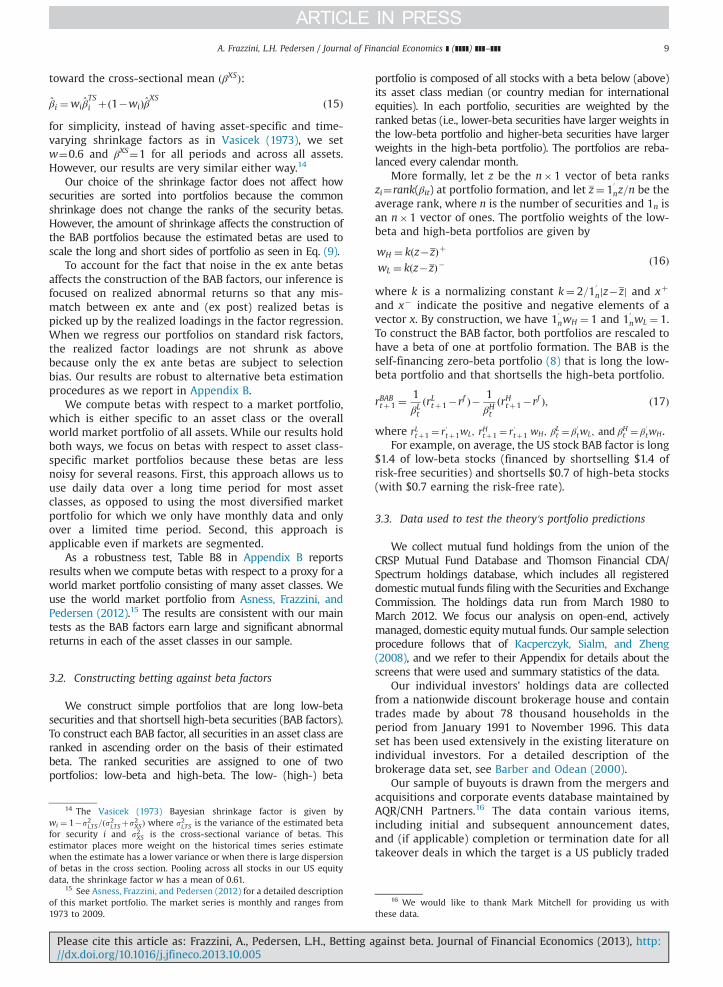
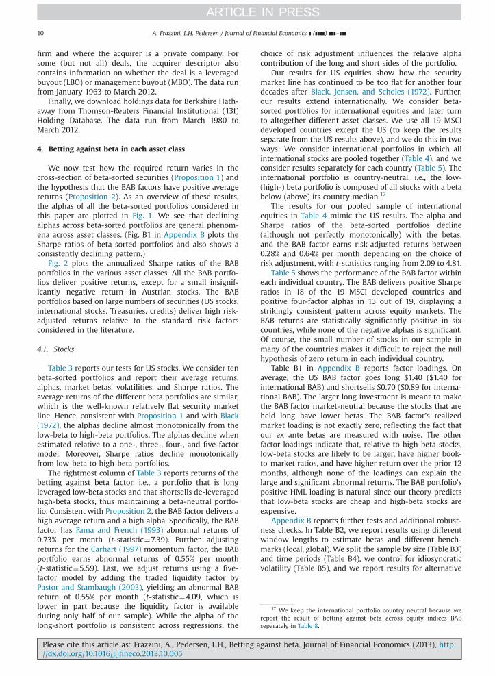
We now test how the required return varies in thecross-section of beta-sorted securities (Proposition 1) andthe hypothesis that the BAB factors have positive averagereturns (Proposition 2). As an overview of these results,the alphas of all the beta-sorted portfolios considered inthis paper are plotted in Fig. 1. We see that decliningalphas across beta-sorted portfolios are general phenom-ena across asset classes. (Fig. B1 in Appendix B plots theSharpe ratios of beta-sorted portfolios and also shows aconsistently declining pattern.)
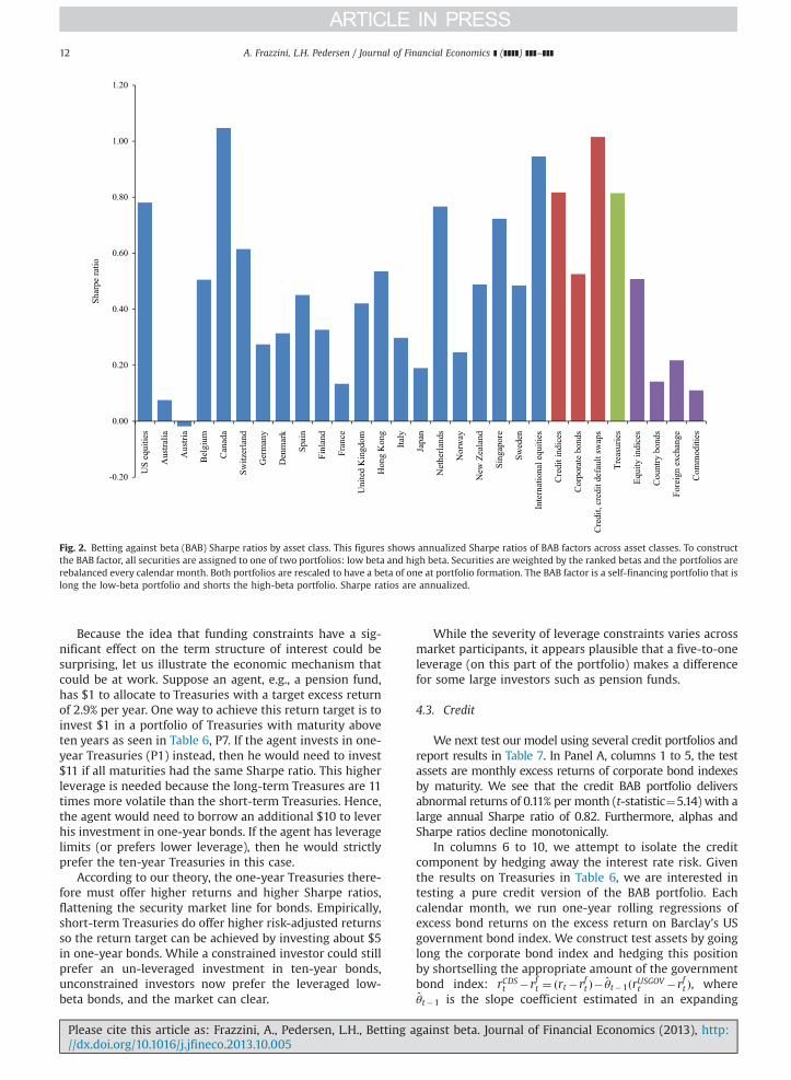
Fig. 2 plots the annualized Sharpe ratios of the BABportfolios in the various asset classes. All the BAB portfo-lios deliver positive returns, except for a small insignif-icantly negative return in Austrian stocks. The BABportfolios based on large numbers of securities (US stocks,international stocks, Treasuries, credits) deliver high risk-adjusted returns relative to the standard risk factorsconsidered in the literature.
4.1. Stocks
Table 3 reports our tests for US stocks. We consider tenbeta-sorted portfolios and report their average returns,alphas, market betas, volatilities, and Sharpe ratios. Theaverage returns of the different beta portfolios are similar,which is the well-known relatively flat security marketline. Hence, consistent with Proposition 1 and with Black(1972), the alphas decline almost monotonically from thelow-beta to high-beta portfolios. The alphas decline whenestimated relative to a one-, three-, four-, and five-factormodel. Moreover, Sharpe ratios decline monotonicallyfrom low-beta to high-beta portfolios.
The rightmost column of Table 3 reports returns of thebetting against beta factor, i.e., a portfolio that is longleveraged low-beta stocks and that shortsells de-leveragedhigh-beta stocks, thus maintaining a beta-neutral portfo-lio. Consistent with Proposition 2, the BAB factor delivers ahigh average return and a high alpha. Specifically, the BABfactor has Fama and French (1993) abnormal returns of0.73% per month (t-statistic¼7.39). Further adjustingreturns for the Carhart (1997) momentum factor, the BABportfolio earns abnormal returns of 0.55% per month(t-statistic¼5.59). Last, we adjust returns using a five-factor model by adding the traded liquidity factor byPastor and Stambaugh (2003), yielding an abnormal BABreturn of 0.55% per month (t-statistic¼4.09, which islower in part because the liquidity factor is availableduring only half of our sample). While the alpha of thelong-short portfolio is consistent across regressions, the
Please cite this article as: Frazzini, A., Pedersen, L.H., Betting a//dx.doi.org/10.1016/j.jfineco.2013.10.005i
choice of risk adjustment influences the relative alphacontribution of the long and short sides of the portfolio.
Our results for US equities show how the securitymarket line has continued to be too flat for another fourdecades after Black, Jensen, and Scholes (1972). Further,our results extend internationally. We consider beta-sorted portfolios for international equities and later turnto altogether different asset classes. We use all 19 MSCIdeveloped countries except the US (to keep the resultsseparate from the US results above), and we do this in twoways: We consider international portfolios in which allinternational stocks are pooled together (Table 4), and weconsider results separately for each country (Table 5). Theinternational portfolio is country-neutral, i.e., the low-(high-) beta portfolio is composed of all stocks with a betabelow (above) its country median.17
The results for our pooled sample of internationalequities in Table 4 mimic the US results. The alpha andSharpe ratios of the beta-sorted portfolios decline(although not perfectly monotonically) with the betas,and the BAB factor earns risk-adjusted returns between0.28% and 0.64% per month depending on the choice ofrisk adjustment, with t-statistics ranging from 2.09 to 4.81.
Table 5 shows the performance of the BAB factor withineach individual country. The BAB delivers positive Sharperatios in 18 of the 19 MSCI developed countries andpositive four-factor alphas in 13 out of 19, displaying astrikingly consistent pattern across equity markets. TheBAB returns are statistically significantly positive in sixcountries, while none of the negative alphas is significant.Of course, the small number of stocks in our sample inmany of the countries makes it difficult to reject the nullhypothesis of zero return in each individual country.
Table B1 in Appendix B reports factor loadings. Onaverage, the US BAB factor goes long $1.40 ($1.40 forinternational BAB) and shortsells $0.70 ($0.89 for interna-tional BAB). The larger long investment is meant to makethe BAB factor market-neutral because the stocks that areheld long have lower betas. The BAB factor's realizedmarket loading is not exactly zero, reflecting the fact thatour ex ante betas are measured with noise. The otherfactor loadings indicate that, relative to high-beta stocks,low-beta stocks are likely to be larger, have higher book-to-market ratios, and have higher return over the prior 12months, although none of the loadings can explain thelarge and significant abnormal returns. The BAB portfolio'spositive HML loading is natural since our theory predictsthat low-beta stocks are cheap and high-beta stocks areexpensive.
Appendix B reports further tests and additional robust-ness checks. In Table B2, we report results using differentwindow lengths to estimate betas and different bench-marks (local, global). We split the sample by size (Table B3)and time periods (Table B4), we control for idiosyncraticvolatility (Table B5), and we report results for alternative
gainst beta. Journal of Financial Economics (2013), http:

Fig. 1. Alphas of beta-sorted portfolios. This figure shows monthly alphas. The test assets are beta-sorted portfolios. At the beginning of each calendarmonth, securities are ranked in ascending order on the basis of their estimated beta at the end of the previous month. The ranked securities are assigned tobeta-sorted portfolios. This figure plots alphas from low beta (left) to high beta (right). Alpha is the intercept in a regression of monthly excess return. Forequity portfolios, the explanatory variables are the monthly returns from Fama and French (1993), Asness and Frazzini (2013), and Carhart (1997)portfolios. For all other portfolios, the explanatory variables are the monthly returns of the market factor. Alphas are in monthly percent.
A. Frazzini, L.H. Pedersen / Journal of Financial Economics ] (]]]]) ]]]–]]] 11
definitions of the risk-free rate (Table B6). Finally, in TableB7 and Fig. B2 we report an out-of-sample test. We collectpricing data from DataStream and for each country inTable 1 we compute a BAB portfolio over sample periodnot covered by the Xpressfeed Global database.18 All of theresults are consistent: Equity portfolios that bet againstbetas earn significant risk-adjusted returns.
4.2. Treasury bonds
Table 6 reports results for US Treasury bonds. As before,we report average excess returns of bond portfoliosformed by sorting on beta in the previous month. In thecross section of Treasury bonds, ranking on betas with
18 DataStream international pricing data start in 1969, and Xpress-feed Global coverage starts in 1984.
Please cite this article as: Frazzini, A., Pedersen, L.H., Betting a//dx.doi.org/10.1016/j.jfineco.2013.10.005i
respect to an aggregate Treasury bond index is empiricallyequivalent to ranking on duration or maturity. Therefore,in Table 6, one can think of the term “beta,” “duration,” or“maturity” in an interchangeable fashion. The right-mostcolumn reports returns of the BAB factor. Abnormalreturns are computed with respect to a one-factor modelin which alpha is the intercept in a regression of monthlyexcess return on an equally weighted Treasury bondexcess market return.
The results show that the phenomenon of a flatter securitymarket line than predicted by the standard CAPM is notlimited to the cross section of stock returns. Consistent withProposition 1, the alphas decline monotonically with beta.Likewise, Sharpe ratios decline monotonically from 0.73 forlow-beta (short-maturity) bonds to 0.31 for high-beta (long-maturity) bonds. Furthermore, the bond BAB portfolio deli-vers abnormal returns of 0.17% per month (t-statistic¼6.26)with a large annual Sharpe ratio of 0.81.
gainst beta. Journal of Financial Economics (2013), http:
-0.20
0.00
0.20
0.40
0.60
0.80
1.00
1.20
US
equi
ties
Aus
tralia
Aus
tria
Bel
gium
Can
ada
Switz
erla
nd
Ger
man
y
Den
mar
k
Spai
n
Finl
and
Fran
ce
Uni
ted
Kin
gdom
Hon
g K
ong
Italy
Japa
n
Net
herla
nds
Nor
way
New
Zea
land
Sing
apor
e
Swed
en
Inte
rnat
iona
l equ
ities
Cre
dit i
ndic
es
Cor
pora
te b
onds
Cre
dit,
cred
it de
faul
t sw
aps
Trea
surie
s
Equi
ty in
dice
s
Cou
ntry
bon
ds
Fore
ign
exch
ange
Com
mod
ities
Shar
pe ra
tio
Fig. 2. Betting against beta (BAB) Sharpe ratios by asset class. This figures shows annualized Sharpe ratios of BAB factors across asset classes. To constructthe BAB factor, all securities are assigned to one of two portfolios: low beta and high beta. Securities are weighted by the ranked betas and the portfolios arerebalanced every calendar month. Both portfolios are rescaled to have a beta of one at portfolio formation. The BAB factor is a self-financing portfolio that islong the low-beta portfolio and shorts the high-beta portfolio. Sharpe ratios are annualized.
A. Frazzini, L.H. Pedersen / Journal of Financial Economics ] (]]]]) ]]]–]]]12
Because the idea that funding constraints have a sig-nificant effect on the term structure of interest could besurprising, let us illustrate the economic mechanism thatcould be at work. Suppose an agent, e.g., a pension fund,has $1 to allocate to Treasuries with a target excess returnof 2.9% per year. One way to achieve this return target is toinvest $1 in a portfolio of Treasuries with maturity aboveten years as seen in Table 6, P7. If the agent invests in one-year Treasuries (P1) instead, then he would need to invest$11 if all maturities had the same Sharpe ratio. This higherleverage is needed because the long-term Treasures are 11times more volatile than the short-term Treasuries. Hence,the agent would need to borrow an additional $10 to leverhis investment in one-year bonds. If the agent has leveragelimits (or prefers lower leverage), then he would strictlyprefer the ten-year Treasuries in this case.
According to our theory, the one-year Treasuries there-fore must offer higher returns and higher Sharpe ratios,flattening the security market line for bonds. Empirically,short-term Treasuries do offer higher risk-adjusted returnsso the return target can be achieved by investing about $5in one-year bonds. While a constrained investor could stillprefer an un-leveraged investment in ten-year bonds,unconstrained investors now prefer the leveraged low-beta bonds, and the market can clear.
Please cite this article as: Frazzini, A., Pedersen, L.H., Betting a//dx.doi.org/10.1016/j.jfineco.2013.10.005i
While the severity of leverage constraints varies acrossmarket participants, it appears plausible that a five-to-oneleverage (on this part of the portfolio) makes a differencefor some large investors such as pension funds.
4.3. Credit
We next test our model using several credit portfolios andreport results in Table 7. In Panel A, columns 1 to 5, the testassets are monthly excess returns of corporate bond indexesby maturity. We see that the credit BAB portfolio deliversabnormal returns of 0.11% per month (t-statistic¼5.14) with alarge annual Sharpe ratio of 0.82. Furthermore, alphas andSharpe ratios decline monotonically.
In columns 6 to 10, we attempt to isolate the creditcomponent by hedging away the interest rate risk. Giventhe results on Treasuries in Table 6, we are interested intesting a pure credit version of the BAB portfolio. Eachcalendar month, we run one-year rolling regressions ofexcess bond returns on the excess return on Barclay's USgovernment bond index. We construct test assets by goinglong the corporate bond index and hedging this positionby shortselling the appropriate amount of the governmentbond index: rCDSt �rft ¼ ðrt�rft Þ� θt�1ðrUSGOVt �rft Þ, whereθt�1 is the slope coefficient estimated in an expanding
gainst beta. Journal of Financial Economics (2013), http:
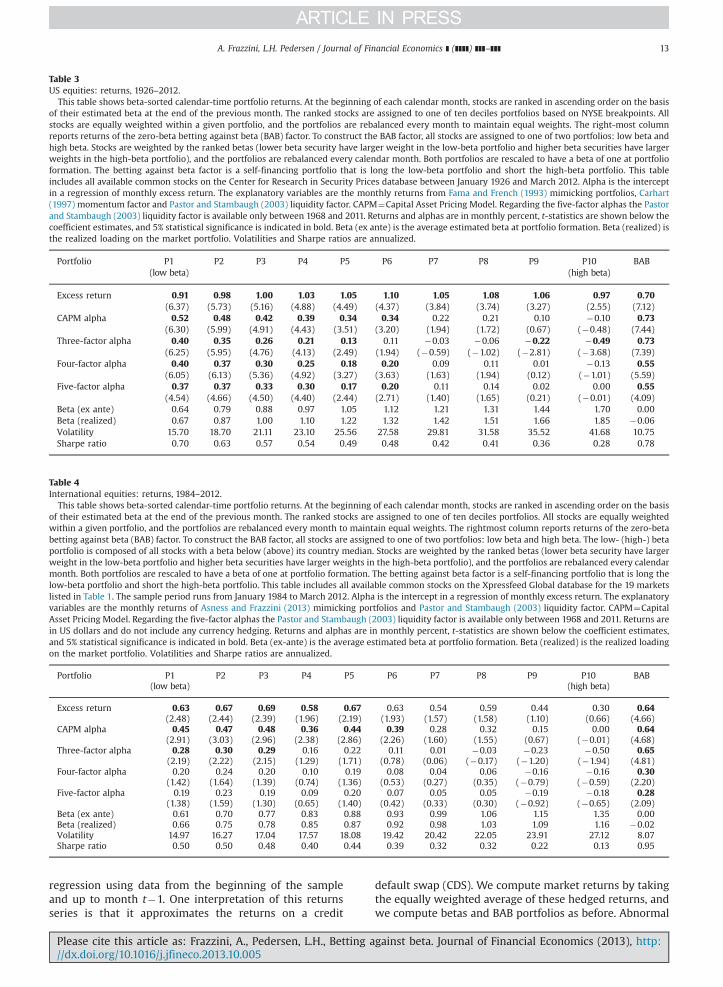
Table 3US equities: returns, 1926–2012.
This table shows beta-sorted calendar-time portfolio returns. At the beginning of each calendar month, stocks are ranked in ascending order on the basisof their estimated beta at the end of the previous month. The ranked stocks are assigned to one of ten deciles portfolios based on NYSE breakpoints. Allstocks are equally weighted within a given portfolio, and the portfolios are rebalanced every month to maintain equal weights. The right-most columnreports returns of the zero-beta betting against beta (BAB) factor. To construct the BAB factor, all stocks are assigned to one of two portfolios: low beta andhigh beta. Stocks are weighted by the ranked betas (lower beta security have larger weight in the low-beta portfolio and higher beta securities have largerweights in the high-beta portfolio), and the portfolios are rebalanced every calendar month. Both portfolios are rescaled to have a beta of one at portfolioformation. The betting against beta factor is a self-financing portfolio that is long the low-beta portfolio and short the high-beta portfolio. This tableincludes all available common stocks on the Center for Research in Security Prices database between January 1926 and March 2012. Alpha is the interceptin a regression of monthly excess return. The explanatory variables are the monthly returns from Fama and French (1993) mimicking portfolios, Carhart(1997) momentum factor and Pastor and Stambaugh (2003) liquidity factor. CAPM¼Capital Asset Pricing Model. Regarding the five-factor alphas the Pastorand Stambaugh (2003) liquidity factor is available only between 1968 and 2011. Returns and alphas are in monthly percent, t-statistics are shown below thecoefficient estimates, and 5% statistical significance is indicated in bold. Beta (ex ante) is the average estimated beta at portfolio formation. Beta (realized) isthe realized loading on the market portfolio. Volatilities and Sharpe ratios are annualized.
Portfolio P1(low beta)
P2 P3 P4 P5 P6 P7 P8 P9 P10(high beta)
BAB
Excess return 0.91 0.98 1.00 1.03 1.05 1.10 1.05 1.08 1.06 0.97 0.70(6.37) (5.73) (5.16) (4.88) (4.49) (4.37) (3.84) (3.74) (3.27) (2.55) (7.12)
CAPM alpha 0.52 0.48 0.42 0.39 0.34 0.34 0.22 0.21 0.10 �0.10 0.73(6.30) (5.99) (4.91) (4.43) (3.51) (3.20) (1.94) (1.72) (0.67) (�0.48) (7.44)
Three-factor alpha 0.40 0.35 0.26 0.21 0.13 0.11 �0.03 �0.06 �0.22 �0.49 0.73(6.25) (5.95) (4.76) (4.13) (2.49) (1.94) (�0.59) (�1.02) (�2.81) (�3.68) (7.39)
Four-factor alpha 0.40 0.37 0.30 0.25 0.18 0.20 0.09 0.11 0.01 �0.13 0.55(6.05) (6.13) (5.36) (4.92) (3.27) (3.63) (1.63) (1.94) (0.12) (�1.01) (5.59)
Five-factor alpha 0.37 0.37 0.33 0.30 0.17 0.20 0.11 0.14 0.02 0.00 0.55(4.54) (4.66) (4.50) (4.40) (2.44) (2.71) (1.40) (1.65) (0.21) (�0.01) (4.09)
Beta (ex ante) 0.64 0.79 0.88 0.97 1.05 1.12 1.21 1.31 1.44 1.70 0.00Beta (realized) 0.67 0.87 1.00 1.10 1.22 1.32 1.42 1.51 1.66 1.85 �0.06Volatility 15.70 18.70 21.11 23.10 25.56 27.58 29.81 31.58 35.52 41.68 10.75Sharpe ratio 0.70 0.63 0.57 0.54 0.49 0.48 0.42 0.41 0.36 0.28 0.78
Table 4International equities: returns, 1984–2012.
This table shows beta-sorted calendar-time portfolio returns. At the beginning of each calendar month, stocks are ranked in ascending order on the basisof their estimated beta at the end of the previous month. The ranked stocks are assigned to one of ten deciles portfolios. All stocks are equally weightedwithin a given portfolio, and the portfolios are rebalanced every month to maintain equal weights. The rightmost column reports returns of the zero-betabetting against beta (BAB) factor. To construct the BAB factor, all stocks are assigned to one of two portfolios: low beta and high beta. The low- (high-) betaportfolio is composed of all stocks with a beta below (above) its country median. Stocks are weighted by the ranked betas (lower beta security have largerweight in the low-beta portfolio and higher beta securities have larger weights in the high-beta portfolio), and the portfolios are rebalanced every calendarmonth. Both portfolios are rescaled to have a beta of one at portfolio formation. The betting against beta factor is a self-financing portfolio that is long thelow-beta portfolio and short the high-beta portfolio. This table includes all available common stocks on the Xpressfeed Global database for the 19 marketslisted in Table 1. The sample period runs from January 1984 to March 2012. Alpha is the intercept in a regression of monthly excess return. The explanatoryvariables are the monthly returns of Asness and Frazzini (2013) mimicking portfolios and Pastor and Stambaugh (2003) liquidity factor. CAPM¼CapitalAsset Pricing Model. Regarding the five-factor alphas the Pastor and Stambaugh (2003) liquidity factor is available only between 1968 and 2011. Returns arein US dollars and do not include any currency hedging. Returns and alphas are in monthly percent, t-statistics are shown below the coefficient estimates,and 5% statistical significance is indicated in bold. Beta (ex-ante) is the average estimated beta at portfolio formation. Beta (realized) is the realized loadingon the market portfolio. Volatilities and Sharpe ratios are annualized.
Portfolio P1(low beta)
P2 P3 P4 P5 P6 P7 P8 P9 P10(high beta)
BAB
Excess return 0.63 0.67 0.69 0.58 0.67 0.63 0.54 0.59 0.44 0.30 0.64(2.48) (2.44) (2.39) (1.96) (2.19) (1.93) (1.57) (1.58) (1.10) (0.66) (4.66)
CAPM alpha 0.45 0.47 0.48 0.36 0.44 0.39 0.28 0.32 0.15 0.00 0.64(2.91) (3.03) (2.96) (2.38) (2.86) (2.26) (1.60) (1.55) (0.67) (�0.01) (4.68)
Three-factor alpha 0.28 0.30 0.29 0.16 0.22 0.11 0.01 �0.03 �0.23 �0.50 0.65(2.19) (2.22) (2.15) (1.29) (1.71) (0.78) (0.06) (�0.17) (�1.20) (�1.94) (4.81)
Four-factor alpha 0.20 0.24 0.20 0.10 0.19 0.08 0.04 0.06 �0.16 �0.16 0.30(1.42) (1.64) (1.39) (0.74) (1.36) (0.53) (0.27) (0.35) (�0.79) (�0.59) (2.20)
Five-factor alpha 0.19 0.23 0.19 0.09 0.20 0.07 0.05 0.05 �0.19 �0.18 0.28(1.38) (1.59) (1.30) (0.65) (1.40) (0.42) (0.33) (0.30) (�0.92) (�0.65) (2.09)
Beta (ex ante) 0.61 0.70 0.77 0.83 0.88 0.93 0.99 1.06 1.15 1.35 0.00Beta (realized) 0.66 0.75 0.78 0.85 0.87 0.92 0.98 1.03 1.09 1.16 �0.02Volatility 14.97 16.27 17.04 17.57 18.08 19.42 20.42 22.05 23.91 27.12 8.07Sharpe ratio 0.50 0.50 0.48 0.40 0.44 0.39 0.32 0.32 0.22 0.13 0.95
A. Frazzini, L.H. Pedersen / Journal of Financial Economics ] (]]]]) ]]]–]]] 13
regression using data from the beginning of the sampleand up to month t�1. One interpretation of this returnsseries is that it approximates the returns on a credit
Please cite this article as: Frazzini, A., Pedersen, L.H., Betting a//dx.doi.org/10.1016/j.jfineco.2013.10.005i
default swap (CDS). We compute market returns by takingthe equally weighted average of these hedged returns, andwe compute betas and BAB portfolios as before. Abnormal
gainst beta. Journal of Financial Economics (2013), http:
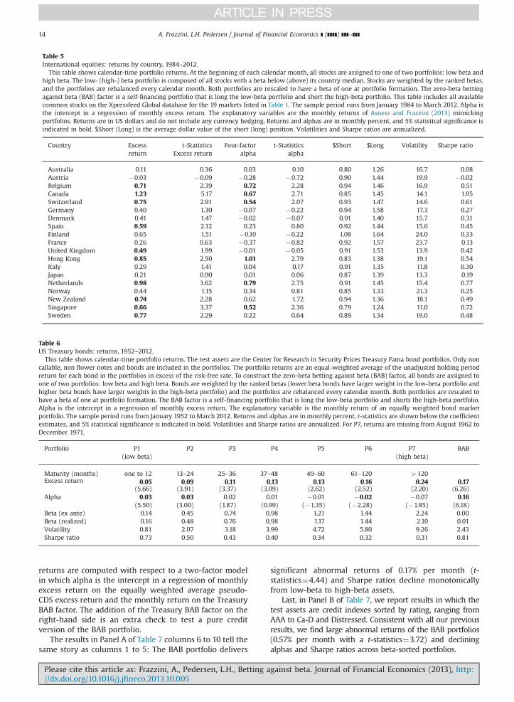
Table 5International equities: returns by country, 1984–2012.
This table shows calendar-time portfolio returns. At the beginning of each calendar month, all stocks are assigned to one of two portfolios: low beta andhigh beta. The low- (high-) beta portfolio is composed of all stocks with a beta below (above) its country median. Stocks are weighted by the ranked betas,and the portfolios are rebalanced every calendar month. Both portfolios are rescaled to have a beta of one at portfolio formation. The zero-beta bettingagainst beta (BAB) factor is a self-financing portfolio that is long the low-beta portfolio and short the high-beta portfolio. This table includes all availablecommon stocks on the Xpressfeed Global database for the 19 markets listed in Table 1. The sample period runs from January 1984 to March 2012. Alpha isthe intercept in a regression of monthly excess return. The explanatory variables are the monthly returns of Asness and Frazzini (2013) mimickingportfolios. Returns are in US dollars and do not include any currency hedging. Returns and alphas are in monthly percent, and 5% statistical significance isindicated in bold. $Short (Long) is the average dollar value of the short (long) position. Volatilities and Sharpe ratios are annualized.
Country Excessreturn
t-StatisticsExcess return
Four-factoralpha
t-Statisticsalpha
$Short $Long Volatility Sharpe ratio
Australia 0.11 0.36 0.03 0.10 0.80 1.26 16.7 0.08Austria �0.03 �0.09 �0.28 �0.72 0.90 1.44 19.9 �0.02Belgium 0.71 2.39 0.72 2.28 0.94 1.46 16.9 0.51Canada 1.23 5.17 0.67 2.71 0.85 1.45 14.1 1.05Switzerland 0.75 2.91 0.54 2.07 0.93 1.47 14.6 0.61Germany 0.40 1.30 �0.07 �0.22 0.94 1.58 17.3 0.27Denmark 0.41 1.47 �0.02 �0.07 0.91 1.40 15.7 0.31Spain 0.59 2.12 0.23 0.80 0.92 1.44 15.6 0.45Finland 0.65 1.51 �0.10 �0.22 1.08 1.64 24.0 0.33France 0.26 0.63 �0.37 �0.82 0.92 1.57 23.7 0.13United Kingdom 0.49 1.99 �0.01 �0.05 0.91 1.53 13.9 0.42Hong Kong 0.85 2.50 1.01 2.79 0.83 1.38 19.1 0.54Italy 0.29 1.41 0.04 0.17 0.91 1.35 11.8 0.30Japan 0.21 0.90 0.01 0.06 0.87 1.39 13.3 0.19Netherlands 0.98 3.62 0.79 2.75 0.91 1.45 15.4 0.77Norway 0.44 1.15 0.34 0.81 0.85 1.33 21.3 0.25New Zealand 0.74 2.28 0.62 1.72 0.94 1.36 18.1 0.49Singapore 0.66 3.37 0.52 2.36 0.79 1.24 11.0 0.72Sweden 0.77 2.29 0.22 0.64 0.89 1.34 19.0 0.48
Table 6US Treasury bonds: returns, 1952–2012.
This table shows calendar-time portfolio returns. The test assets are the Center for Research in Security Prices Treasury Fama bond portfolios. Only noncallable, non flower notes and bonds are included in the portfolios. The portfolio returns are an equal-weighted average of the unadjusted holding periodreturn for each bond in the portfolios in excess of the risk-free rate. To construct the zero-beta betting against beta (BAB) factor, all bonds are assigned toone of two portfolios: low beta and high beta. Bonds are weighted by the ranked betas (lower beta bonds have larger weight in the low-beta portfolio andhigher beta bonds have larger weights in the high-beta portfolio) and the portfolios are rebalanced every calendar month. Both portfolios are rescaled tohave a beta of one at portfolio formation. The BAB factor is a self-financing portfolio that is long the low-beta portfolio and shorts the high-beta portfolio.Alpha is the intercept in a regression of monthly excess return. The explanatory variable is the monthly return of an equally weighted bond marketportfolio. The sample period runs from January 1952 to March 2012. Returns and alphas are in monthly percent, t-statistics are shown below the coefficientestimates, and 5% statistical significance is indicated in bold. Volatilities and Sharpe ratios are annualized. For P7, returns are missing from August 1962 toDecember 1971.
Portfolio P1(low beta)
P2 P3 P4 P5 P6 P7(high beta)
BAB
Maturity (months) one to 12 13–24 25–36 37–48 49–60 61–120 4120Excess return 0.05 0.09 0.11 0.13 0.13 0.16 0.24 0.17
(5.66) (3.91) (3.37) (3.09) (2.62) (2.52) (2.20) (6.26)Alpha 0.03 0.03 0.02 0.01 �0.01 �0.02 �0.07 0.16
(5.50) (3.00) (1.87) (0.99) (�1.35) (�2.28) (�1.85) (6.18)Beta (ex ante) 0.14 0.45 0.74 0.98 1.21 1.44 2.24 0.00Beta (realized) 0.16 0.48 0.76 0.98 1.17 1.44 2.10 0.01Volatility 0.81 2.07 3.18 3.99 4.72 5.80 9.26 2.43Sharpe ratio 0.73 0.50 0.43 0.40 0.34 0.32 0.31 0.81
A. Frazzini, L.H. Pedersen / Journal of Financial Economics ] (]]]]) ]]]–]]]14
returns are computed with respect to a two-factor modelin which alpha is the intercept in a regression of monthlyexcess return on the equally weighted average pseudo-CDS excess return and the monthly return on the TreasuryBAB factor. The addition of the Treasury BAB factor on theright-hand side is an extra check to test a pure creditversion of the BAB portfolio.
The results in Panel A of Table 7 columns 6 to 10 tell thesame story as columns 1 to 5: The BAB portfolio delivers
Please cite this article as: Frazzini, A., Pedersen, L.H., Betting a//dx.doi.org/10.1016/j.jfineco.2013.10.005i
significant abnormal returns of 0.17% per month (t-statistics¼4.44) and Sharpe ratios decline monotonicallyfrom low-beta to high-beta assets.
Last, in Panel B of Table 7, we report results in which thetest assets are credit indexes sorted by rating, ranging fromAAA to Ca-D and Distressed. Consistent with all our previousresults, we find large abnormal returns of the BAB portfolios(0.57% per month with a t-statistics¼3.72) and decliningalphas and Sharpe ratios across beta-sorted portfolios.
gainst beta. Journal of Financial Economics (2013), http:
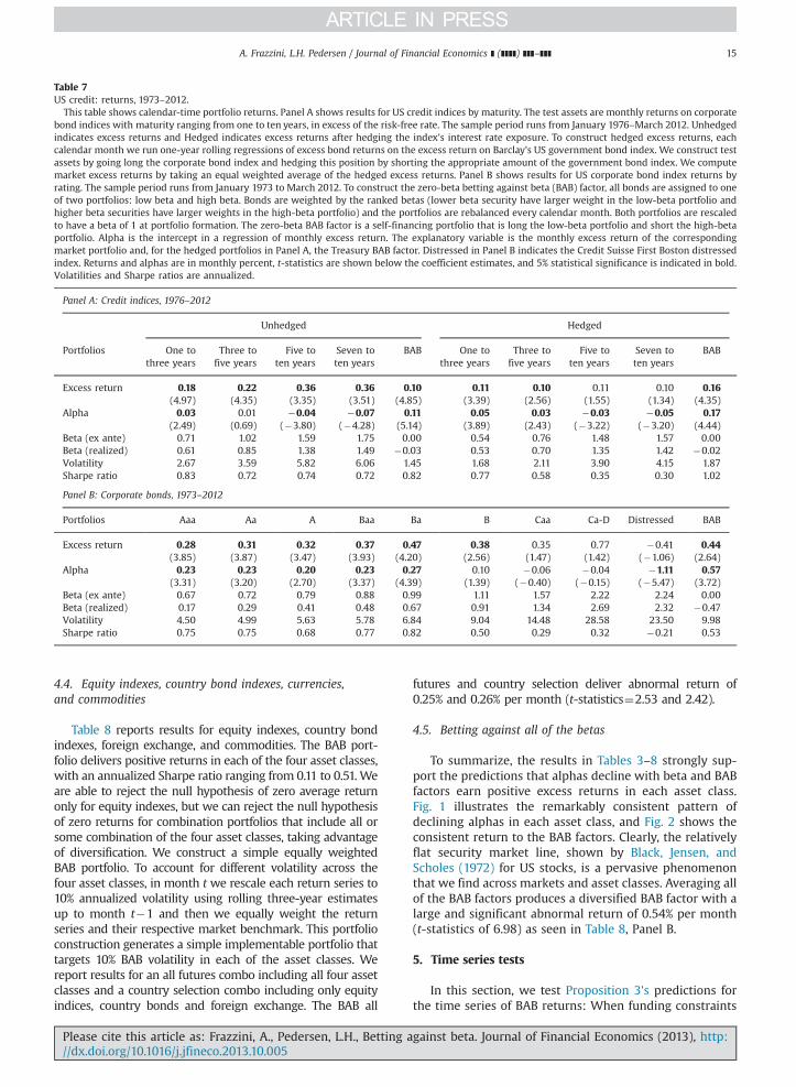
Table 7US credit: returns, 1973–2012.
This table shows calendar-time portfolio returns. Panel A shows results for US credit indices by maturity. The test assets are monthly returns on corporatebond indices with maturity ranging from one to ten years, in excess of the risk-free rate. The sample period runs from January 1976–March 2012. Unhedgedindicates excess returns and Hedged indicates excess returns after hedging the index's interest rate exposure. To construct hedged excess returns, eachcalendar month we run one-year rolling regressions of excess bond returns on the excess return on Barclay's US government bond index. We construct testassets by going long the corporate bond index and hedging this position by shorting the appropriate amount of the government bond index. We computemarket excess returns by taking an equal weighted average of the hedged excess returns. Panel B shows results for US corporate bond index returns byrating. The sample period runs from January 1973 to March 2012. To construct the zero-beta betting against beta (BAB) factor, all bonds are assigned to oneof two portfolios: low beta and high beta. Bonds are weighted by the ranked betas (lower beta security have larger weight in the low-beta portfolio andhigher beta securities have larger weights in the high-beta portfolio) and the portfolios are rebalanced every calendar month. Both portfolios are rescaledto have a beta of 1 at portfolio formation. The zero-beta BAB factor is a self-financing portfolio that is long the low-beta portfolio and short the high-betaportfolio. Alpha is the intercept in a regression of monthly excess return. The explanatory variable is the monthly excess return of the correspondingmarket portfolio and, for the hedged portfolios in Panel A, the Treasury BAB factor. Distressed in Panel B indicates the Credit Suisse First Boston distressedindex. Returns and alphas are in monthly percent, t-statistics are shown below the coefficient estimates, and 5% statistical significance is indicated in bold.Volatilities and Sharpe ratios are annualized.
Panel A: Credit indices, 1976–2012
Unhedged Hedged
Portfolios One tothree years
Three tofive years
Five toten years
Seven toten years
BAB One tothree years
Three tofive years
Five toten years
Seven toten years
BAB
Excess return 0.18 0.22 0.36 0.36 0.10 0.11 0.10 0.11 0.10 0.16(4.97) (4.35) (3.35) (3.51) (4.85) (3.39) (2.56) (1.55) (1.34) (4.35)
Alpha 0.03 0.01 �0.04 �0.07 0.11 0.05 0.03 �0.03 �0.05 0.17(2.49) (0.69) (�3.80) (�4.28) (5.14) (3.89) (2.43) (�3.22) (�3.20) (4.44)
Beta (ex ante) 0.71 1.02 1.59 1.75 0.00 0.54 0.76 1.48 1.57 0.00Beta (realized) 0.61 0.85 1.38 1.49 �0.03 0.53 0.70 1.35 1.42 �0.02Volatility 2.67 3.59 5.82 6.06 1.45 1.68 2.11 3.90 4.15 1.87Sharpe ratio 0.83 0.72 0.74 0.72 0.82 0.77 0.58 0.35 0.30 1.02
Panel B: Corporate bonds, 1973–2012
Portfolios Aaa Aa A Baa Ba B Caa Ca-D Distressed BAB
Excess return 0.28 0.31 0.32 0.37 0.47 0.38 0.35 0.77 �0.41 0.44(3.85) (3.87) (3.47) (3.93) (4.20) (2.56) (1.47) (1.42) (�1.06) (2.64)
Alpha 0.23 0.23 0.20 0.23 0.27 0.10 �0.06 �0.04 �1.11 0.57(3.31) (3.20) (2.70) (3.37) (4.39) (1.39) (�0.40) (�0.15) (�5.47) (3.72)
Beta (ex ante) 0.67 0.72 0.79 0.88 0.99 1.11 1.57 2.22 2.24 0.00Beta (realized) 0.17 0.29 0.41 0.48 0.67 0.91 1.34 2.69 2.32 �0.47Volatility 4.50 4.99 5.63 5.78 6.84 9.04 14.48 28.58 23.50 9.98Sharpe ratio 0.75 0.75 0.68 0.77 0.82 0.50 0.29 0.32 �0.21 0.53
A. Frazzini, L.H. Pedersen / Journal of Financial Economics ] (]]]]) ]]]–]]] 15
4.4. Equity indexes, country bond indexes, currencies,and commodities
Table 8 reports results for equity indexes, country bondindexes, foreign exchange, and commodities. The BAB port-folio delivers positive returns in each of the four asset classes,with an annualized Sharpe ratio ranging from 0.11 to 0.51. Weare able to reject the null hypothesis of zero average returnonly for equity indexes, but we can reject the null hypothesisof zero returns for combination portfolios that include all orsome combination of the four asset classes, taking advantageof diversification. We construct a simple equally weightedBAB portfolio. To account for different volatility across thefour asset classes, in month t we rescale each return series to10% annualized volatility using rolling three-year estimatesup to month t�1 and then we equally weight the returnseries and their respective market benchmark. This portfolioconstruction generates a simple implementable portfolio thattargets 10% BAB volatility in each of the asset classes. Wereport results for an all futures combo including all four assetclasses and a country selection combo including only equityindices, country bonds and foreign exchange. The BAB all
Please cite this article as: Frazzini, A., Pedersen, L.H., Betting a//dx.doi.org/10.1016/j.jfineco.2013.10.005i
futures and country selection deliver abnormal return of0.25% and 0.26% per month (t-statistics¼2.53 and 2.42).
4.5. Betting against all of the betas
To summarize, the results in Tables 3–8 strongly sup-port the predictions that alphas decline with beta and BABfactors earn positive excess returns in each asset class.Fig. 1 illustrates the remarkably consistent pattern ofdeclining alphas in each asset class, and Fig. 2 shows theconsistent return to the BAB factors. Clearly, the relativelyflat security market line, shown by Black, Jensen, andScholes (1972) for US stocks, is a pervasive phenomenonthat we find across markets and asset classes. Averaging allof the BAB factors produces a diversified BAB factor with alarge and significant abnormal return of 0.54% per month(t-statistics of 6.98) as seen in Table 8, Panel B.
5. Time series tests
In this section, we test Proposition 3's predictions forthe time series of BAB returns: When funding constraints
gainst beta. Journal of Financial Economics (2013), http:
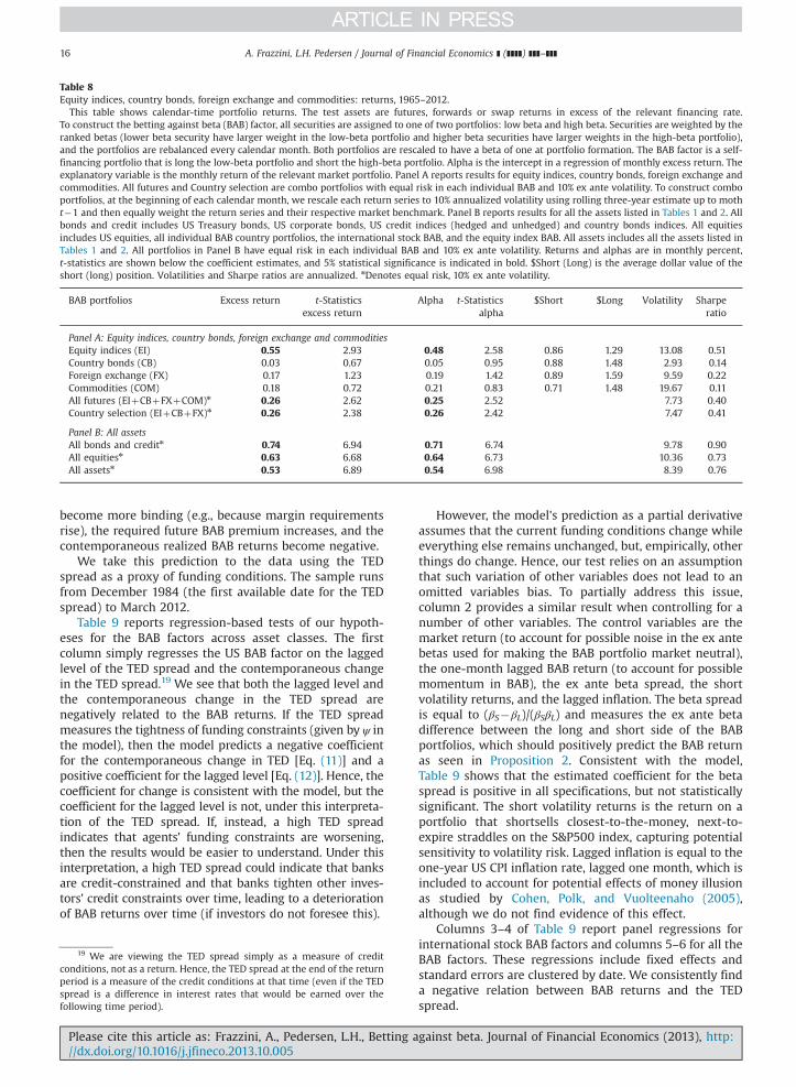
Table 8Equity indices, country bonds, foreign exchange and commodities: returns, 1965–2012.
This table shows calendar-time portfolio returns. The test assets are futures, forwards or swap returns in excess of the relevant financing rate.To construct the betting against beta (BAB) factor, all securities are assigned to one of two portfolios: low beta and high beta. Securities are weighted by theranked betas (lower beta security have larger weight in the low-beta portfolio and higher beta securities have larger weights in the high-beta portfolio),and the portfolios are rebalanced every calendar month. Both portfolios are rescaled to have a beta of one at portfolio formation. The BAB factor is a self-financing portfolio that is long the low-beta portfolio and short the high-beta portfolio. Alpha is the intercept in a regression of monthly excess return. Theexplanatory variable is the monthly return of the relevant market portfolio. Panel A reports results for equity indices, country bonds, foreign exchange andcommodities. All futures and Country selection are combo portfolios with equal risk in each individual BAB and 10% ex ante volatility. To construct comboportfolios, at the beginning of each calendar month, we rescale each return series to 10% annualized volatility using rolling three-year estimate up to motht�1 and then equally weight the return series and their respective market benchmark. Panel B reports results for all the assets listed in Tables 1 and 2. Allbonds and credit includes US Treasury bonds, US corporate bonds, US credit indices (hedged and unhedged) and country bonds indices. All equitiesincludes US equities, all individual BAB country portfolios, the international stock BAB, and the equity index BAB. All assets includes all the assets listed inTables 1 and 2. All portfolios in Panel B have equal risk in each individual BAB and 10% ex ante volatility. Returns and alphas are in monthly percent,t-statistics are shown below the coefficient estimates, and 5% statistical significance is indicated in bold. $Short (Long) is the average dollar value of theshort (long) position. Volatilities and Sharpe ratios are annualized. nDenotes equal risk, 10% ex ante volatility.
BAB portfolios Excess return t-Statisticsexcess return
Alpha t-Statisticsalpha
$Short $Long Volatility Sharperatio
Panel A: Equity indices, country bonds, foreign exchange and commoditiesEquity indices (EI) 0.55 2.93 0.48 2.58 0.86 1.29 13.08 0.51Country bonds (CB) 0.03 0.67 0.05 0.95 0.88 1.48 2.93 0.14Foreign exchange (FX) 0.17 1.23 0.19 1.42 0.89 1.59 9.59 0.22Commodities (COM) 0.18 0.72 0.21 0.83 0.71 1.48 19.67 0.11All futures (EIþCBþFXþCOM)n 0.26 2.62 0.25 2.52 7.73 0.40Country selection (EIþCBþFX)n 0.26 2.38 0.26 2.42 7.47 0.41
Panel B: All assetsAll bonds and creditn 0.74 6.94 0.71 6.74 9.78 0.90All equitiesn 0.63 6.68 0.64 6.73 10.36 0.73All assetsn 0.53 6.89 0.54 6.98 8.39 0.76
A. Frazzini, L.H. Pedersen / Journal of Financial Economics ] (]]]]) ]]]–]]]16
become more binding (e.g., because margin requirementsrise), the required future BAB premium increases, and thecontemporaneous realized BAB returns become negative.
We take this prediction to the data using the TEDspread as a proxy of funding conditions. The sample runsfrom December 1984 (the first available date for the TEDspread) to March 2012.
Table 9 reports regression-based tests of our hypoth-eses for the BAB factors across asset classes. The firstcolumn simply regresses the US BAB factor on the laggedlevel of the TED spread and the contemporaneous changein the TED spread.19 We see that both the lagged level andthe contemporaneous change in the TED spread arenegatively related to the BAB returns. If the TED spreadmeasures the tightness of funding constraints (given by ψ inthe model), then the model predicts a negative coefficientfor the contemporaneous change in TED [Eq. (11)] and apositive coefficient for the lagged level [Eq. (12)]. Hence, thecoefficient for change is consistent with the model, but thecoefficient for the lagged level is not, under this interpreta-tion of the TED spread. If, instead, a high TED spreadindicates that agents' funding constraints are worsening,then the results would be easier to understand. Under thisinterpretation, a high TED spread could indicate that banksare credit-constrained and that banks tighten other inves-tors' credit constraints over time, leading to a deteriorationof BAB returns over time (if investors do not foresee this).
19 We are viewing the TED spread simply as a measure of creditconditions, not as a return. Hence, the TED spread at the end of the returnperiod is a measure of the credit conditions at that time (even if the TEDspread is a difference in interest rates that would be earned over thefollowing time period).
Please cite this article as: Frazzini, A., Pedersen, L.H., Betting a//dx.doi.org/10.1016/j.jfineco.2013.10.005i
However, the model's prediction as a partial derivativeassumes that the current funding conditions change whileeverything else remains unchanged, but, empirically, otherthings do change. Hence, our test relies on an assumptionthat such variation of other variables does not lead to anomitted variables bias. To partially address this issue,column 2 provides a similar result when controlling for anumber of other variables. The control variables are themarket return (to account for possible noise in the ex antebetas used for making the BAB portfolio market neutral),the one-month lagged BAB return (to account for possiblemomentum in BAB), the ex ante beta spread, the shortvolatility returns, and the lagged inflation. The beta spreadis equal to (βS�βL)/(βSβL) and measures the ex ante betadifference between the long and short side of the BABportfolios, which should positively predict the BAB returnas seen in Proposition 2. Consistent with the model,Table 9 shows that the estimated coefficient for the betaspread is positive in all specifications, but not statisticallysignificant. The short volatility returns is the return on aportfolio that shortsells closest-to-the-money, next-to-expire straddles on the S&P500 index, capturing potentialsensitivity to volatility risk. Lagged inflation is equal to theone-year US CPI inflation rate, lagged one month, which isincluded to account for potential effects of money illusionas studied by Cohen, Polk, and Vuolteenaho (2005),although we do not find evidence of this effect.
Columns 3–4 of Table 9 report panel regressions forinternational stock BAB factors and columns 5–6 for all theBAB factors. These regressions include fixed effects andstandard errors are clustered by date. We consistently finda negative relation between BAB returns and the TEDspread.
gainst beta. Journal of Financial Economics (2013), http:
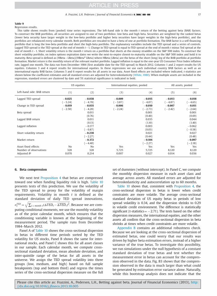
Table 9Regression results.
This table shows results from (pooled) time series regressions. The left-hand side is the month t return of the betting against beta (BAB) factors.To construct the BAB portfolios, all securities are assigned to one of two portfolios: low beta and high beta. Securities are weighted by the ranked betas(lower beta security have larger weight in the low-beta portfolio and higher beta securities have larger weights in the high-beta portfolio), and theportfolios are rebalanced every calendar month. Both portfolios are rescaled to have a beta of one at portfolio formation. The BAB factor is a self-financingportfolio that is long the low-beta portfolio and short the high-beta portfolio. The explanatory variables include the TED spread and a series of controls.Lagged TED spread is the TED spread at the end of month t�1. Change in TED spread is equal to TED spread at the end of month t minus Ted spread at theend of month t�1. Short volatility return is the month t return on a portfolio that shorts at-the-money straddles on the S&P 500 index. To construct theshort volatility portfolio, on index options expiration dates we write the next-to-expire closest-to-maturity straddle on the S&P 500 index and hold it tomaturity. Beta spread is defined as (HBeta�LBeta)/(HBetan LBeta) where HBeta (LBeta) are the betas of the short (long) leg of the BAB portfolio at portfolioformation. Market return is the monthly return of the relevant market portfolio. Lagged inflation is equal to the one-year US Consumer Price Index inflationrate, lagged one month. The data run from December 1984 (first available date for the TED spread) to March 2012. Columns 1 and 2 report results for USequities. Columns 3 and 4 report results for international equities. In these regressions we use each individual country BAB factors as well as aninternational equity BAB factor. Columns 5 and 6 report results for all assets in our data. Asset fixed effects are included where indicated, t-statistics areshown below the coefficient estimates and all standard errors are adjusted for heteroskedasticity (White, 1980). When multiple assets are included in theregression, standard errors are clustered by date and 5% statistical significance is indicated in bold.
US equities International equities, pooled All assets, pooled
Left-hand side: BAB return (1) (2) (3) (4) (5) (6)
Lagged TED spread �0.025 �0.038 �0.009 �0.015 �0.013 �0.018(�5.24) (�4.78) (�3.87) (�4.07) (�4.87) (�4.65)
Change in TED spread �0.019 �0.035 �0.006 �0.010 �0.007 �0.011(�2.58) (�4.28) (�2.24) (�2.73) (�2.42) (�2.64)
Beta spread 0.011 0.001 0.001(0.76) (0.40) (0.69)
Lagged BAB return 0.011 0.035 0.044(0.13) (1.10) (1.40)
Lagged inflation �0.177 0.003 �0.062(�0.87) (0.03) (�0.58)
Short volatility return �0.238 0.021 0.027(�2.27) (0.44) (0.48)
Market return �0.372 �0.104 �0.097(�4.40) (�2.27) (�2.18)
Asset fixed effects No No Yes Yes Yes YesNumber of observations 328 328 5,725 5,725 8,120 8,120Adjusted R² 0.070 0.214 0.007 0.027 0.014 0.036
A. Frazzini, L.H. Pedersen / Journal of Financial Economics ] (]]]]) ]]]–]]] 17
6. Beta compression
We next test Proposition 4 that betas are compressedtoward one when funding liquidity risk is high. Table 10presents tests of this prediction. We use the volatility ofthe TED spread to proxy for the volatility of marginrequirements. Volatility in month t is defined as thestandard deviation of daily TED spread innovations,
sTEDt ¼ffiffiffiffiffiffiffiffiffiffiffiffiffiffiffiffiffiffiffiffiffiffiffiffiffiffiffiffiffiffiffiffiffiffiffiffiffiffiffiffiffiffiffiffiffiffiffiffiffiffiffiffiffiffiffiffiffiffiffiffiffi∑sAmonth tðΔTEDs�ΔTEDtÞ2
q. Because we are com-
puting conditional moments, we use the monthly volatilityas of the prior calendar month, which ensures that theconditioning variable is known at the beginning of themeasurement period. The sample runs from December1984–March 2012.
Panel A of Table 10 shows the cross-sectional dispersionin betas in different time periods sorted by the TEDvolatility for US stocks, Panel B shows the same for inter-national stocks, and Panel C shows this for all asset classesin our sample. Each calendar month, we compute cross-sectional standard deviation, mean absolute deviation, andinter-quintile range of the betas for all assets in theuniverse. We assign the TED spread volatility into threegroups (low, medium, and high) based on full samplebreakpoints (top and bottom third) and regress the timesseries of the cross-sectional dispersion measure on the full
Please cite this article as: Frazzini, A., Pedersen, L.H., Betting a//dx.doi.org/10.1016/j.jfineco.2013.10.005i
set of dummies (without intercept). In Panel C, we computethe monthly dispersion measure in each asset class andaverage across assets. All standard errors are adjusted forheteroskedasticity and autocorrelation up to 60 months.
Table 10 shows that, consistent with Proposition 4, thecross-sectional dispersion in betas is lower when creditconstraints are more volatile. The average cross-sectionalstandard deviation of US equity betas in periods of lowspread volatility is 0.34, and the dispersion shrinks to 0.29in volatile credit environment. The difference is statisticallysignificant (t-statistics¼�2.71). The tests based on the otherdispersion measures, the international equities, and the otherassets all confirm that the cross-sectional dispersion in betashrinks at times when credit constraints are more volatile.
Appendix B contains an additional robustness check.Because we are looking at the cross-sectional dispersion ofestimated betas, one could worry that our results wasdriven by higher beta estimation errors, instead of a highervariance of the true betas. To investigate this possibility,we run simulations under the null hypothesis of a constantstandard deviation of true betas and test whether themeasurement error in betas can account for the compres-sion observed in the data. Fig. B3 shows that the compres-sion observed in the data is much larger than what couldbe generated by estimation error variance alone. Naturally,while this bootstrap analysis does not indicate that the
gainst beta. Journal of Financial Economics (2013), http:
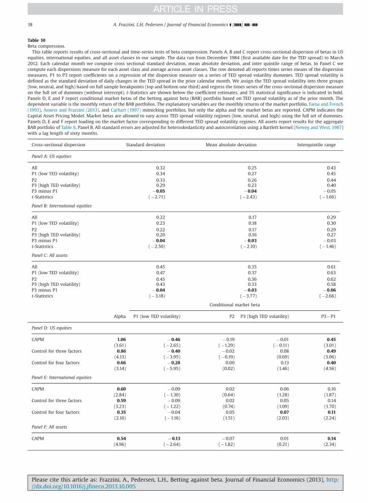
Table 10Beta compression.
This table reports results of cross-sectional and time-series tests of beta compression. Panels A, B and C report cross-sectional dispersion of betas in USequities, international equities, and all asset classes in our sample. The data run from December 1984 (first available date for the TED spread) to March2012. Each calendar month we compute cross sectional standard deviation, mean absolute deviation, and inter quintile range of betas. In Panel C wecompute each dispersions measure for each asset class and average across asset classes. The row denoted all reports times series means of the dispersionmeasures. P1 to P3 report coefficients on a regression of the dispersion measure on a series of TED spread volatility dummies. TED spread volatility isdefined as the standard deviation of daily changes in the TED spread in the prior calendar month. We assign the TED spread volatility into three groups(low, neutral, and high) based on full sample breakpoints (top and bottom one third) and regress the times series of the cross-sectional dispersion measureon the full set of dummies (without intercept). t-Statistics are shown below the coefficient estimates, and 5% statistical significance is indicated in bold.Panels D, E and F report conditional market betas of the betting against beta (BAB) portfolio based on TED spread volatility as of the prior month. Thedependent variable is the monthly return of the BAB portfolios. The explanatory variables are the monthly returns of the market portfolio, Fama and French(1993), Asness and Frazzini (2013), and Carhart (1997) mimicking portfolios, but only the alpha and the market betas are reported. CAPM indicates theCapital Asset Pricing Model. Market betas are allowed to vary across TED spread volatility regimes (low, neutral, and high) using the full set of dummies.Panels D, E and F report loading on the market factor corresponding to different TED spread volatility regimes. All assets report results for the aggregateBAB portfolio of Table 9, Panel B. All standard errors are adjusted for heteroskedasticity and autocorrelation using a Bartlett kernel (Newey and West, 1987)with a lag length of sixty months.
Cross-sectional dispersion Standard deviation Mean absolute deviation Interquintile range
Panel A: US equities
All 0.32 0.25 0.43P1 (low TED volatility) 0.34 0.27 0.45P2 0.33 0.26 0.44P3 (high TED volatility) 0.29 0.23 0.40P3 minus P1 �0.05 �0.04 �0.05t-Statistics (�2.71) (�2.43) (�1.66)
Panel B: International equities
All 0.22 0.17 0.29P1 (low TED volatility) 0.23 0.18 0.30P2 0.22 0.17 0.29P3 (high TED volatility) 0.20 0.16 0.27P3 minus P1 �0.04 �0.03 �0.03t-Statistics (�2.50) (�2.10) (�1.46)
Panel C: All assets
All 0.45 0.35 0.61P1 (low TED volatility) 0.47 0.37 0.63P2 0.45 0.36 0.62P3 (high TED volatility) 0.43 0.33 0.58P3 minus P1 �0.04 �0.03 �0.06t-Statistics (�3.18) (�3.77) (�2.66)
Conditional market beta
Alpha P1 (low TED volatility) P2 P3 (high TED volatility) P3�P1
Panel D: US equities
CAPM 1.06 �0.46 �0.19 �0.01 0.45(3.61) (�2.65) (�1.29) (�0.11) (3.01)
Control for three factors 0.86 �0.40 �0.02 0.08 0.49(4.13) (�3.95) (�0.19) (0.69) (3.06)
Control for four factors 0.66 �0.28 0.00 0.13 0.40(3.14) (�5.95) (0.02) (1.46) (4.56)
Panel E: International equities
CAPM 0.60 �0.09 0.02 0.06 0.16(2.84) (�1.30) (0.64) (1.28) (1.87)
Control for three factors 0.59 �0.09 0.02 0.05 0.14(3.23) (�1.22) (0.74) (1.09) (1.70)
Control for four factors 0.35 �0.04 0.05 0.07 0.11(2.16) (�1.16) (1.51) (2.03) (2.24)
Panel F: All assets
CAPM 0.54 �0.13 �0.07 0.01 0.14(4.96) (�2.64) (�1.82) (0.21) (2.34)
Please cite this article as: Frazzini, A., Pedersen, L.H., Betting against beta. Journal of Financial Economics (2013), http://dx.doi.org/10.1016/j.jfineco.2013.10.005i
A. Frazzini, L.H. Pedersen / Journal of Financial Economics ] (]]]]) ]]]–]]]18
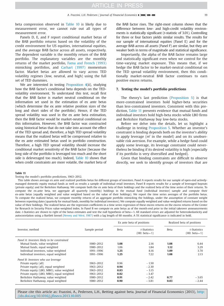
A. Frazzini, L.H. Pedersen / Journal of Financial Economics ] (]]]]) ]]]–]]] 19
beta compression observed in Table 10 is likely due tomeasurement error, we cannot rule out all types ofmeasurement error.
Panels D, E, and F report conditional market betas ofthe BAB portfolio returns based on the volatility of thecredit environment for US equities, international equities,and the average BAB factor across all assets, respectively.The dependent variable is the monthly return of the BABportfolio. The explanatory variables are the monthlyreturns of the market portfolio, Fama and French (1993)mimicking portfolios, and Carhart (1997) momentumfactor. Market betas are allowed to vary across TEDvolatility regimes (low, neutral, and high) using the fullset of TED dummies.
We are interested in testing Proposition 4(ii), studyinghow the BAB factor's conditional beta depends on the TED-volatility environment. To understand this test, recall firstthat the BAB factor is market neutral conditional on theinformation set used in the estimation of ex ante betas(which determine the ex ante relative position sizes of thelong and short sides of the portfolio). Hence, if the TEDspread volatility was used in the ex ante beta estimation,then the BAB factor would be market-neutral conditional onthis information. However, the BAB factor was constructedusing historical betas that do not take into account the effectof the TED spread and, therefore, a high TED spread volatilitymeans that the realized betas will be compressed relative tothe ex ante estimated betas used in portfolio construction.Therefore, a high TED spread volatility should increase theconditional market sensitivity of the BAB factor (because thelong side of the portfolio is leveraged too much and the shortside is deleveraged too much). Indeed, Table 10 shows thatwhen credit constraints are more volatile, the market beta of
Table 11Testing the model's portfolio predictions, 1963–2012.
This table shows average ex ante and realized portfolio betas for different groumanaged domestic equity mutual funds as well as results a sample of individual(private equity) and for Berkshire Hathaway. We compute both the ex ante beta ocompute the ex-ante beta, we aggregate all quarterly (monthly) holdingsex-ante betas (equally weighted and value weighted based on the value of thTo compute the realized betas, we compute monthly returns of an aggregate pobetween reporting dates (quarterly for mutual funds, monthly for individual investovalue of their holdings. The realized betas are the regression coefficients in a timefor Research in Security Prices value-weighted index. In Panel B we compute ex adate. t-Statistics are shown to right of the betas estimates and test the null hypotautocorrelation using a Bartlett kernel (Newey and West, 1987) with a lag length
Investor, method Sample period
Panel A: Investors likely to be constrainedMutual funds, value weighted 1980–2012Mutual funds, equal weighted 1980–2012Individual investors, value weighted 1991–1996Individual investors, equal weighted 1991–1996
Panel B: Investors who use leveragePrivate equity (all) 1963–2012Private equity (all), equal weighted 1963–2012Private equity (LBO, MBO), value weighted 1963–2012Private equity (LBO, MBO), equal weighted 1963–2012Berkshire Hathaway, value weighted 1980–2012Berkshire Hathaway, equal weighted 1980–2012
Please cite this article as: Frazzini, A., Pedersen, L.H., Betting a//dx.doi.org/10.1016/j.jfineco.2013.10.005i
the BAB factor rises. The right-most column shows that thedifference between low- and high-credit volatility environ-ments is statistically significant (t-statistic of 3.01). Controllingfor three or four factors yields similar results. The results forour sample of international equities (Panel E) and for theaverage BAB across all assets (Panel F) are similar, but they areweaker both in terms of magnitude and statistical significance.
Importantly, the alpha of the BAB factor remains largeand statistically significant even when we control for thetime-varying market exposure. This means that, if wehedge the BAB factor to be market-neutral conditional onthe TED spread volatility environment, then this condi-tionally market-neutral BAB factor continues to earnpositive excess returns.
7. Testing the model's portfolio predictions
The theory's last prediction (Proposition 5) is thatmore-constrained investors hold higher-beta securitiesthan less-constrained investors. Consistent with this pre-diction, Table 11 presents evidence that mutual funds andindividual investors hold high-beta stocks while LBO firmsand Berkshire Hathaway buy low-beta stocks.
Before we delve into the details, let us highlight achallenge in testing Proposition 5. Whether an investor'sconstraint is binding depends both on the investor's abilityto apply leverage (mi in the model) and on its unobser-vable risk aversion. For example, while a hedge fund couldapply some leverage, its leverage constraint could never-theless be binding if its desired volatility is high (especiallyif its portfolio is very diversified and hedged).
Given that binding constraints are difficult to observedirectly, we seek to identify groups of investors that are
ps of investors. Panel A reports results for our sample of open-end actively-retail investors. Panel B reports results for a sample of leveraged buyoutsf their holdings and the realized beta of the time series of their returns. Toin the mutual fund (individual investor) sample and compute theireir holdings). We report the time series averages of the portfolio betas.rtfolio mimicking the holdings, under the assumption of constant weightrs). We compute equally weighted and value-weighted returns based on theseries regression of these excess returns on the excess returns of the Centernte betas as of the month-end prior to the initial takeover announcementshesis of beta¼1. All standard errors are adjusted for heteroskedasticity andof 60 months. A 5% statistical significance is indicated in bold.
Ex ante beta of positions Realized beta of positions
Beta t-Statistics(H0: beta¼1)
Beta t-Statistics(H0: beta¼1)
1.08 2.16 1.08 6.441.06 1.84 1.12 3.291.25 8.16 1.09 3.701.25 7.22 1.08 2.13
0.96 �1.500.94 �2.300.83 �3.150.82 �3.470.91 �2.42 0.77 �3.650.90 �3.81 0.83 �2.44
gainst beta. Journal of Financial Economics (2013), http:
20 As further consistent evidence, younger people and people withless financial wealth (who might be more constrained) tend to ownportfolios with higher betas (Calvet, Campbell, and Sodini, 2007, Table 5).Further, consistent with the idea that leverage requires certain skills andsophistication, Grinblatt, Keloharju, and Linnainmaa (2011) report thatindividuals with low intelligence scores hold higher-beta portfolios thanindividuals with high intelligence scores.
A. Frazzini, L.H. Pedersen / Journal of Financial Economics ] (]]]]) ]]]–]]]20
plausibly constrained and unconstrained. One example ofan investor that could be constrained is a mutual fund. The1940 Investment Company Act places some restriction onmutual funds' use of leverage, and many mutual funds areprohibited by charter from using leverage. A mutual funds'need to hold cash to meet redemptions (mi41 in themodel) creates a further incentive to overweight high-betasecurities. Overweighting high-beta stocks helps avoidlagging their benchmark in a bull market because of thecash holdings (some funds use futures contracts to “equi-tize” the cash, but other funds are not allowed to usederivative contracts).
A second class of investors that could face borrowingconstraints is individual retail investors. Although we donot have direct evidence of their inability to employleverage (and some individuals certainly do), we thinkthat (at least in aggregate) it is plausible that they arelikely to face borrowing restrictions.
The flipside of this portfolio test is identifying relativelyunconstrained investors. Thus, one needs investors thatcould be allowed to use leverage and are operating belowtheir leverage cap so that their leverage constraints are notbinding. We look at the holdings of two groups ofinvestors that could satisfy these criteria as they haveaccess to leverage and focus on long equity investments(requiring less leverage than long/short strategies).
First, we look at the firms that are the target of bids byleveraged buyout (LBO) funds and other forms of privateequity. These investors, as the name suggest, employleverage to acquire a public company. Admittedly, we donot have direct evidence of the maximum leverageavailable to these LBO firms relative to the leverage theyapply, but anecdotal evidence suggests that they achievea substantial amount of leverage.
Second, we examine the holdings of Berkshire Hath-away, a publicly traded corporation run by Warren Buffettthat holds a diversified portfolio of equities and employsleverage (by issuing debt, via insurance float, and othermeans). The advantage of using the holdings of a publiccorporation that holds equities such as Berkshire is that wecan directly observe its leverage. Over the period fromMarch 1980 to March 2012, its average book leverage,defined as (book equityþtotal debt) / book equity, wasabout 1.2, that is, 20% borrowing, and the market leverageincluding other liabilities such insurance float was about1.6 (Frazzini, Kabiller, and Pedersen, 2012). It is thereforeplausible to assume that Berkshire at the margin couldissue more debt but choose not to, making it a likelycandidate for an investor whose combination of riskaversion and borrowing constraints made it relativelyunconstrained during our sample period.
Table 11 reports the results of our portfolio test.We estimate both the ex ante beta of the various investors'holdings and the realized beta of the time series of theirreturns. We first aggregate all holdings for each investorgroup, compute their ex-ante betas (equal and valueweighted, respectively), and take the time series average.To compute the realized betas, we compute monthlyreturns of an aggregate portfolio mimicking the holdings,under the assumption of constant weight between report-ing dates. The realized betas are the regression coefficients
Please cite this article as: Frazzini, A., Pedersen, L.H., Betting a//dx.doi.org/10.1016/j.jfineco.2013.10.005i
in a time series regression of these excess returns on theexcess returns of the CRSP value-weighted index.
Panel A shows evidence consistent with the hypothesisthat constrained investors stretch for return by increasingtheir betas. Mutual funds hold securities with betas aboveone, and we are able to reject the null hypothesis of betasbeing equal to one. These findings are consistent withthose of Karceski (2002), but our sample is much larger,including all funds over 30-year period. Similar evidence ispresented for individual retail investors: Individual inves-tors tend to hold securities with betas that are significantlyabove one.20
Panel B reports results for our sample of private equity.For each target stock in our database, we focus on itsex ante beta as of the month-end prior to the initialannouncements date. This focus is to avoid confoundingeffects that result from changes in betas related to theactual delisting event. We consider both the sample of allprivate equity deals and the subsample that we are able topositively identify as LBO/MBO events. Since we only havepartial information about whether each deal is a LBO/MBO,the broad sample includes all types of deals where acompany is taken private. The results are consistent withProposition 5 in that investors executing leverage buyoutstend to acquire (or attempt to acquire in case of a non-successful bid) firms with low betas, and we are able toreject the null hypothesis of a unit beta.
The results for Berkshire Hathaway show a similarpattern: Warren Buffett bets against beta by buying stockswith betas significantly below one and applying leverage.
8. Conclusion
All real-world investors face funding constraints suchas leverage constraints and margin requirements, andthese constraints influence investors' required returnsacross securities and over time. We find empirically thatportfolios of high-beta assets have lower alphas andSharpe ratios than portfolios of low-beta assets. Thesecurity market line is not only flatter than predicted bythe standard CAPM for US equities (as reported by Black,Jensen, and Scholes (1972)), but we also find this relativeflatness in 18 of 19 international equity markets, inTreasury markets, for corporate bonds sorted by maturityand by rating, and in futures markets. We show how thisdeviation from the standard CAPM can be captured usingbetting against beta factors, which could also be useful ascontrol variables in future research (Proposition 2). Thereturn of the BAB factor rivals those of all the standardasset pricing factors (e.g., value, momentum, and size) interms of economic magnitude, statistical significance, androbustness across time periods, subsamples of stocks, andglobal asset classes.
gainst beta. Journal of Financial Economics (2013), http:
A. Frazzini, L.H. Pedersen / Journal of Financial Economics ] (]]]]) ]]]–]]] 21
Extending the Black (1972) model, we consider theimplications of funding constraints for cross-sectional andtime series asset returns. We show that worsening fundingliquidity should lead to losses for the BAB factor in thetime series (Proposition 3) and that increased fundingliquidity risk compresses betas in the cross section ofsecurities toward one (Proposition 4), and we find con-sistent evidence empirically.
Our model also has implications for agents' portfolioselection (Proposition 5). To test this, we identify investorsthat are likely to be relatively constrained and uncon-strained. We discuss why mutual funds and individualinvestors could be leverage constrained, and, consistentwith the model's prediction that constrained investors gofor riskier assets, we find that these investor groups holdportfolios with betas above one on average.
Conversely, we show that leveraged buyout funds andBerkshire Hathaway, all of which have access to leverage,buy stocks with betas below one on average, anotherprediction of the model. Hence, these investors could betaking advantage of the BAB effect by applying leverage tosafe assets and being compensated by investors facingborrowing constraints who take the other side. Buffett betsagainst beta as Fisher Black believed one should.
Appendix A. Analysis and proofs
Before we prove our propositions, we provide a basicanalysis of portfolio selection with constraints. This ana-lysis is based on Fig. A1. The top panel shows the mean-standard deviation frontier for an agent with mo1, that is,an agent who can use leverage. We see that the agent canleverage the tangency portfolio T to arrive at the portfolioT . To achieve a higher expected return, the agent needs toleverage riskier assets, which gives rise to the hyperbolasegment to the right of T . The agent in the graph isassumed to have risk preferences giving rise to the optimalportfolio C. Hence, the agent is leverage constrained so hechooses to apply leverage to portfolio C instead of thetangency portfolio.
The bottom panel of Fig. A1 similarly shows the mean-standard deviation frontier for an agent with m41, that is,an agent who must hold some cash. If the agent keeps theminimum amount of money in cash and invests the rest inthe tangency portfolio, then he arrives at portfolio T′.To achieve higher expected return, the agent must investin riskier assets and, in the depicted case, he invests incash and portfolio D, arriving at portfolio D′.
Unconstrained investors invest in the tangency portfo-lio and cash. Hence, the market portfolio is a weightedaverage of T and riskier portfolios such as C and D.Therefore, the market portfolio is riskier than the tangencyportfolio.
A.1. Proof of Proposition 1
Rearranging the equilibrium-price Eq. (7) yields
Etðrstþ1Þ ¼ rf þψ tþγ1Pste′sΩxn
Please cite this article as: Frazzini, A., Pedersen, L.H., Betting a//dx.doi.org/10.1016/j.jfineco.2013.10.005i
¼ rf þψ tþγ1PstcovtðPs
tþ1þδstþ1; Ptþ1þδtþ1� �
′xnÞ
¼ rf þψ tþγcovtðrstþ1; rMtþ1ÞP′
txn ð18Þ
where es is a vector with a one in row s and zeroselsewhere. Multiplying this equation by the market port-folio weights ws ¼ xnsPs
t=∑jxnjPjt and summing over s gives
EtðrMtþ1Þ ¼ rf þψ tþγvartðrMtþ1ÞP′tx
n ð19Þ
that is,
γP′tx
n ¼ λtvartðrMtþ1Þ
ð20Þ
Inserting this into Eq. (18) gives the first result in theproposition. The second result follows from writing theexpected return as
Etðrstþ1Þ�rf ¼ ψ tð1�βst Þþβst ðEtðrMtþ1Þ�rf Þ ð21Þ
and noting that the first term is (Jensen's) alpha. Turningto the third result regarding efficient portfolios, the Sharperatio increases in beta until the tangency portfolio isreached and decreases thereafter. Hence, the last resultfollows from the fact that the tangency portfolio has a betaless than one. This is true because the market portfolio isan average of the tangency portfolio (held by uncon-strained agents) and riskier portfolios (held by constrainedagents) so the market portfolio is riskier than the tangencyportfolio. Hence, the tangency portfolio must have a lowerexpected return and beta (strictly lower if and only if someagents are constrained). □
A.2. Proof of Propositions 2–3
The expected return of the BAB factor is
EtðrBABtþ1Þ ¼1βLt
ðEtðrLtþ1Þ�rf Þ� 1βHt
ðEtðrHtþ1Þ�rf Þ
¼ 1βLt
ðψ tþβLt λtÞ�1βHt
ðψ tþβHt λtÞ
¼ βHt �βLtβLtβ
Ht
ψ t ð22Þ
Consider next a change in mkt . Such a change in a time
t margin requirement does not change the time t betas fortwo reasons. First, it does not affect the distribution ofprices in the following period tþ1. Second, prices at timet are scaled (up or down) by the same proportion due tothe change in Lagrange multipliers as seen in Eq. (7).Hence, all returns from t to tþ1 change by the samemultiplier, leading to time t betas staying the same.
Given Eq. (22), Eq. (12) in the proposition now followsif we can show that ψt increases in mk because this lead to
∂EtðrBABtþ1Þ∂mk
t
¼ βHt �βLtβLtβ
Ht
∂ψ t
∂mkt
40 ð23Þ
Further, because prices move opposite required returns,Eq. (11) then follows. To see that an increase in mk
tincreases ψt, note that the constrained agents' assetexpenditure decreases with a higher mk
t . Indeed, summingthe portfolio constraint across constrained agents [where
gainst beta. Journal of Financial Economics (2013), http:
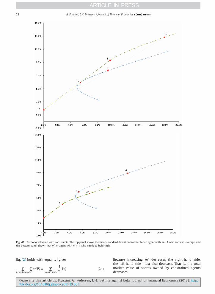
Fig. A1. Portfolio selection with constraints. The top panel shows the mean-standard deviation frontier for an agent with mo1 who can use leverage, andthe bottom panel shows that of an agent with m41 who needs to hold cash.
A. Frazzini, L.H. Pedersen / Journal of Financial Economics ] (]]]]) ]]]–]]]22
Eq. (2) holds with equality] gives
∑i constrained
∑sxi;sPs
t ¼ ∑i constrained
1mi
Wit ð24Þ
Please cite this article as: Frazzini, A., Pedersen, L.H., Betting a//dx.doi.org/10.1016/j.jfineco.2013.10.005i
Because increasing mk decreases the right-hand side,the left-hand side must also decrease. That is, the totalmarket value of shares owned by constrained agentsdecreases.
gainst beta. Journal of Financial Economics (2013), http:
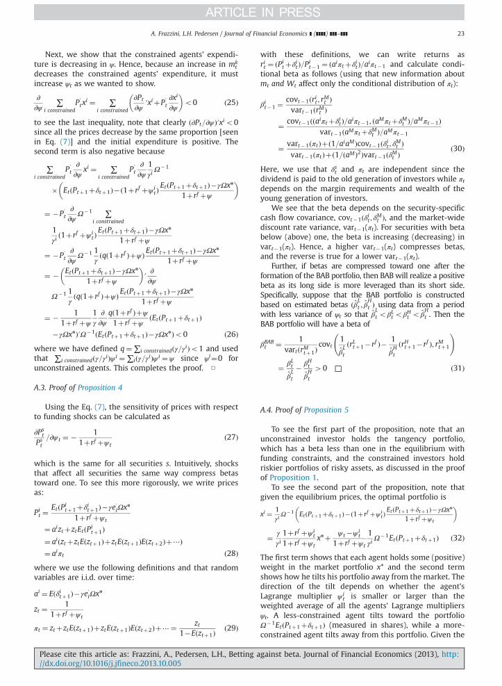
A. Frazzini, L.H. Pedersen / Journal of Financial Economics ] (]]]]) ]]]–]]] 23
Next, we show that the constrained agents' expendi-ture is decreasing in ψ. Hence, because an increase in mk
tdecreases the constrained agents' expenditure, it mustincrease ψt as we wanted to show.
∂∂ψ
∑i constrained
P′tx
i ¼ ∑i constrained
∂Pt
∂ψ′xiþP′
t∂xi
∂ψ
� �o0 ð25Þ
to see the last inequality, note that clearly ð∂Pt=∂ψÞ′xio0since all the prices decrease by the same proportion [seenin Eq. (7)] and the initial expenditure is positive. Thesecond term is also negative because
∑i constrained
P′t∂∂ψ
xi ¼ ∑i constrained
P′t∂∂ψ
1γiΩ�1
� EtðPtþ1þδtþ1Þ�ð1þrf þψ itÞEtðPtþ1þδtþ1Þ�γΩxn
1þrf þψ
� �
¼ �P′t∂∂ψ
Ω�1 ∑i constrained
1γið1þrf þψ i
tÞEtðPtþ1þδtþ1Þ�γΩxn
1þrf þψ
¼ �P′t∂∂ψ
Ω�1 1γðqð1þrf ÞþψÞ EtðPtþ1þδtþ1Þ�γΩxn
1þrf þψ
¼ � EtðPtþ1þδtþ1Þ�γΩxn
1þrf þψ
� �′∂∂ψ
Ω�1 1γðqð1þrf ÞþψÞ EtðPtþ1þδtþ1Þ�γΩxn
1þrf þψ
¼ � 11þrf þψ
1γ
∂∂ψ
qð1þrf Þþψ
1þrf þψðEtðPtþ1þδtþ1Þ
�γΩxnÞ′Ω�1ðEtðPtþ1þδtþ1Þ�γΩxnÞo0 ð26Þwhere we have defined q¼∑i constrainedðγ=γiÞo1 and usedthat ∑i constrainedðγ=γiÞψ i ¼∑iðγ=γiÞψ i ¼ ψ since ψi¼0 forunconstrained agents. This completes the proof. □
A.3. Proof of Proposition 4
Using the Eq. (7), the sensitivity of prices with respectto funding shocks can be calculated as
∂Pst
Pst=∂ψ t ¼ � 1
1þrf þψ tð27Þ
which is the same for all securities s. Intuitively, shocksthat affect all securities the same way compress betastoward one. To see this more rigorously, we write pricesas:
Pit ¼
EtðPitþ1þδitþ1Þ�γe′iΩxn
1þrf þψ t
¼ aiztþztEtðPitþ1Þ
¼ aiðztþztEðztþ1ÞþztEðztþ1ÞEðztþ2Þþ⋯Þ¼ aiπt ð28Þ
where we use the following definitions and that randomvariables are i.i.d. over time:
ai ¼ Eðδitþ1Þ�γe′iΩxn
zt ¼1
1þrf þψ t
πt ¼ ztþztEðztþ1ÞþztEðztþ1ÞEðztþ2Þþ⋯¼ zt1�Eðztþ1Þ
ð29Þ
Please cite this article as: Frazzini, A., Pedersen, L.H., Betting a//dx.doi.org/10.1016/j.jfineco.2013.10.005i
with these definitions, we can write returns asrit ¼ ðPi
tþδitÞ=Pit�1 ¼ ðaiπtþδitÞ=aiπt�1 and calculate condi-
tional beta as follows (using that new information aboutmt and Wt affect only the conditional distribution of πt):
βit�1 ¼covt�1ðrit ; rMt Þvart�1ðrMt Þ
¼ covt�1ððaiπtþδitÞ=aiπt�1; ðaMπtþδMt Þ=aMπt�1Þvart�1ðaMπtþδMt Þ=aMπt�1
¼ vart�1ðπtÞþð1=aiaMÞcovt�1ðδit ; δMt Þvart�1ðπtÞþð1=ðaMÞ2Þvart�1ðδMt Þ
ð30Þ
Here, we use that δst and πt are independent since thedividend is paid to the old generation of investors while πtdepends on the margin requirements and wealth of theyoung generation of investors.
We see that the beta depends on the security-specificcash flow covariance, covt�1ðδit ; δMt Þ, and the market-widediscount rate variance, vart�1(πt). For securities with betabelow (above) one, the beta is increasing (decreasing) invart�1(πt). Hence, a higher vart�1(πt) compresses betas,and the reverse is true for a lower vart�1(πt).
Further, if betas are compressed toward one after theformation of the BAB portfolio, then BAB will realize a positivebeta as its long side is more leveraged than its short side.Specifically, suppose that the BAB portfolio is constructedbased on estimated betas ðβLt ; β
Ht Þ using data from a period
with less variance of ψt so that βLt oβLt oβHt o β
Ht . Then the
BAB portfolio will have a beta of
βBABt ¼ 1vartðrMtþ1Þ
covt1
βLt
ðrLtþ1�rf Þ� 1
βHt
ðrHtþ1�rf Þ; rMtþ1
!
¼ βLt
βLt
� βHt
βHt
40 □ ð31Þ
A.4. Proof of Proposition 5
To see the first part of the proposition, note that anunconstrained investor holds the tangency portfolio,which has a beta less than one in the equilibrium withfunding constraints, and the constrained investors holdriskier portfolios of risky assets, as discussed in the proofof Proposition 1.
To see the second part of the proposition, note thatgiven the equilibrium prices, the optimal portfolio is
xi ¼ 1γiΩ�1 EtðPtþ1þδtþ1Þ�ð1þrf þψ i
tÞEtðPtþ1þδtþ1Þ�γΩxn
1þrf þψ t
� �
¼ γ
γi1þrf þψ i
t
1þrf þψ txnþ ψ t�ψ i
t
1þrf þψ t
1γiΩ�1EtðPtþ1þδtþ1Þ ð32Þ
The first term shows that each agent holds some (positive)weight in the market portfolio x* and the second termshows how he tilts his portfolio away from the market. Thedirection of the tilt depends on whether the agent'sLagrange multiplier ψ i
t is smaller or larger than theweighted average of all the agents' Lagrange multipliersψt. A less-constrained agent tilts toward the portfolioΩ�1EtðPtþ1þδtþ1Þ (measured in shares), while a more-constrained agent tilts away from this portfolio. Given the
gainst beta. Journal of Financial Economics (2013), http:

A. Frazzini, L.H. Pedersen / Journal of Financial Economics ] (]]]]) ]]]–]]]24
expression (13), we can write the variance-covariancematrix as
Ω¼ s2Mbb′þΣ ð33Þwhere Σ¼var(e) and s2M ¼ varðPM
tþ1Þ. Using the MatrixInversion Lemma (the Sherman-Morrison-Woodbury for-mula), the tilt portfolio can be written as
Ω�1EtðPtþ1þδtþ1Þ
¼ Σ�1�Σ�1bb′Σ�1 1s2Mþb′Σ�1b
!EtðPtþ1þδtþ1Þ
¼ Σ�1EtðPtþ1þδtþ1Þ�Σ�1bb′Σ�1EtðPtþ1þδtþ1Þ1
s2Mþb′Σ�1b
¼ Σ�1EtðPtþ1þδtþ1Þ�yΣ�1b ð34Þ
where y¼ b′Σ�1EtðPtþ1þδtþ1Þ=ðs2Mþb′Σ�1bÞ is a scalar.It holds that ðΣ�1bÞs4ðΣ�1bÞk because bs4bk and becauses and k have the same variances and covariances in Σ,implying that (Σ�1)s,j¼(Σ�1)k,j for jas,k and (Σ�1)s,s¼(Σ�1)k,kZ(Σ�1)s,k¼(Σ�1)k,s. Similarly, it holds that[Σ�1Et(Ptþ1þδtþ1)]so[Σ�1Et(Ptþ1þδtþ1)]k since a highermarket exposure leads to a lower price (as seen below).So, everything else equal, a higher b leads to a lower weightin the tilt portfolio.
Finally, security s also has a higher return beta than kbecause
βit ¼PMt covðPi
tþ1þδitþ1; PMtþ1þδMtþ1Þ
PitvarðPM
tþ1þδMtþ1Þ¼ PM
t
Pit
bi ð35Þ
and a higher bi means a lower price:
Pit ¼
EtðPitþ1þδitþ1Þ�γðΩxnÞi
1þrf þψ t
¼ EtðPitþ1þδitþ1Þ�γðΣxnÞi�bib′xnγs2M
1þrf þψ t□ ð36Þ
Appendix B and C
See the internet appendix at http://jfe.rochester.edu/appendix.htm
References
Acharya, V.V., Pedersen, L.H., 2005. Asset pricing with liquidity risk.J. Financial Econ. 77, 375–410.
Ang, A., Hodrick, R., Xing, Y., Zhang, X., 2006. The cross-section ofvolatility and expected returns. J. Finance 61, 259–299.
Ang, A., Hodrick, R., Xing, Y., Zhang, X., 2009. High idiosyncratic volatilityand low returns: international and further US evidence. J. FinancialEcon. 91, 1–23.
Ashcraft, A., Garleanu, N., Pedersen, L.H., 2010. Two monetary tools: interestrates and hair cuts. NBER Macroeconomics Annu. 25, 143–180.
Asness, C., Frazzini, A., 2013. The devil in HML's details. J. Portfol. Manage.39, 49–68.
Asness, C., Frazzini, A., Pedersen, L.H., 2012. Leverage aversion and riskparity. Financial Anal. J. 68 (1), 47–59.
Baker, M., Bradley, B., Wurgler, J., 2011. Benchmarks as limits to arbitrage:understanding the low volatility anomaly. Financial Anal. J. 67 (1),40–54.
Bali, T., Cakici, N., Whitelaw, R., 2011. Maxing out: stocks as lotteries andthe cross-section of expected returns. J. Financial Econ. 99 (2),427–446.
Please cite this article as: Frazzini, A., Pedersen, L.H., Betting a//dx.doi.org/10.1016/j.jfineco.2013.10.005i
Barber, B., Odean, T., 2000. Trading is hazardous to your wealth: thecommon stock investment performance of individual investors.J. Finance 55, 773–806.
Black, F., 1972. Capital market equilibrium with restricted borrowing.J. Bus. 45 (3), 444–455.
Black, F., 1993. Beta and return. J. Portfol. Manage. 20, 8–18.Black, F., Jensen, M.C., Scholes, M., 1972. The capital asset pricing model:
some empirical tests. In: Jensen, M.C. (Ed.), Studies in the Theory ofCapital Markets, Praeger, New York, NY, pp. 79–121.
Brennan, M.J., 1971. Capital market equilibriumwith divergent borrowingand lending rates. J. Financial Quant. Anal. 6, 1197–1205.
Brennan, M.J., 1993. Agency and asset pricing. Unpublished workingpaper. University of California, Los Angeles, CA.
Brunnermeier, M., Pedersen, L.H., 2009. Market liquidity and fundingliquidity. Rev. Financial Stud. 22, 2201–2238.
Calvet, L.E., Campbell, J.Y., Sodini, P., 2007. Down or out: assessing thewelfare costs of household investment mistakes. J. Political Econ. 115(5), 707–747.
Carhart, M., 1997. On persistence in mutual fund performance. J. Finance52, 57–82.
Cohen, R.B., Polk, C., Vuolteenaho, T., 2005. Money illusion in the stockmarket: the Modigliani-Cohn hypothesis. Q. J. Econ. 120 (2), 639–668.
Cuoco, D., 1997. Optimal consumption and equilibrium prices withportfolio constraints and stochastic income. J. Econ. Theory. 72 (1),33–73.
De Santis, G., Gerard, B., 1997. International asset pricing and portfoliodiversification with time-varying risk. J. Finance 52, 1881–1912.
Duffee, G., 2010. Sharpe ratios in term structure models. Unpublishedworking paper. Johns Hopkins University, Baltimore, MD.
Elton, E.G., Gruber, M.J., Brown, S.J., Goetzmannn, W., 2003. ModernPortfolio Theory and Investment Analysis. Wiley, Hoboken, NJ.
Falkenstein, E.G., 1994. Mutual Funds, Idiosyncratic Variance, and AssetReturns. Northwestern University, IL (dissertation).
Fama, E.F., 1984. The information in the term structure. J. Financial Econ.13, 509–528.
Fama, E.F., 1986. Term premiums and default premiums in moneymarkets. J. Financial Econ. 17, 175–196.
Fama, E.F., French, K.R., 1992. The cross-section of expected stock returns.J. Finance 47 (2), 427–465.
Fama, E.F., French, K.R., 1993. Common risk factors in the returns onstocks and bonds. J. Financial Econ. 33, 3–56.
Fama, E.F., French, K.R., 1996. Multifactor explanations of asset pricinganomalies. J. Finance 51, 55–84.
Frazzini, A., Kabiller, D., Pedersen, L.H., 2012. Buffett's Alpha. Unpublishedworking paper. AQR Capital Management and New York University,Greenwich, CT and New York, NY.
Fu, F., 2009. Idiosyncratic risk and the cross-section of expected stockreturns. J. Financial Econ. 91 (1), 24–37.
Garleanu, N., Pedersen, L.H., 2011. Margin-based asset pricing anddeviations from the law of one price. Rev. Financial Stud. 24 (6),1980–2022.
Gibbons, M., 1982. Multivariate tests of financial models: a new approach.J. Financial Econ. 10, 3–27.
Grinblatt, M., Keloharju, M., Linnainmaa, J., 2011. IQ and stock marketparticipation. J. Finance 66 (6), 2121–2164.
Gromb, D., Vayanos, D., 2002. Equilibrium and welfare in markets withfinancially constrained arbitrageurs. J. Financial Econ. 66, 361–407.
Hindy, A., 1995. Viable prices in financial markets with solvency con-straints. J. Math. Econ. 24 (2), 105–135.
Kacperczyk, M., Sialm, C., Zheng, L., 2008. Unobserved actions of mutualfunds. Rev. Financial Stud. 21, 2379–2416.
Kandel, S., 1984. The likelihood ratio test statistic of mean-varianceefficiency without a riskless asset. J. Financial Econ. 13, 575–592.
Karceski, J., 2002. Returns-chasing behavior, mutual funds, and beta'sdeath. J. Financial Quan. Anal. 37 (4), 559–594.
Lewellen, J., Nagel, S., 2006. The conditional CAPM does not explain asset-pricing anomalies. J. Financial Econ. 82 (2), 289–314.
Mehrling, P., 2005. Fischer Black and the Revolutionary Idea of Finance.Wiley, Hoboken, NJ.
Merton, R.C., 1980. On estimating the expected return on the market: anexploratory investigation. J. Financial Econ. 8, 323–361.
Moskowitz, T., Ooi, Y.H., Pedersen, L.H., 2012. Time series momentum.J. Financial Econ. 104 (2), 228–250.
Newey, W.K., West, K.D., 1987. A simple, positive semi-definite, hetero-skedasticity and autocorrelation consistent covariance matrix. Econ-ometrica 55 (3), 703–708.
Pastor, L., Stambaugh, R., 2003. Liquidity risk and expected stock returns.J. Political Econ. 111, 642–685.
gainst beta. Journal of Financial Economics (2013), http:

A. Frazzini, L.H. Pedersen / Journal of Financial Economics ] (]]]]) ]]]–]]] 25
Polk, C., Thompson, S., Vuolteenaho, T., 2006. Cross-sectional forecasts ofthe equity premium. J. Financial Econ. 81, 101–141.
Shanken, J., 1985. Multivariate tests of the zero-beta CAPM. J. FinancialEcon. 14, 327–348.
Tobin, J., 1958. Liquidity preference as behavior toward risk. R.. Econ.Stud. 25, 65–86.
Please cite this article as: Frazzini, A., Pedersen, L.H., Betting a//dx.doi.org/10.1016/j.jfineco.2013.10.005i
Vasicek, O.A., 1973. A note on using cross-sectional information inBayesian estimation on security beta's. J. Finance 28 (5), 1233–1239.
White, H., 1980. A heteroskedasticity-consistent covariance matrix esti-mator and a direct test for heteroskedasticity. Econometrica 48 (4),817–838.
gainst beta. Journal of Financial Economics (2013), http: