Journal of English Linguistics - Faculteit der Letteren ... · Nevertheless, the analyses yield...
74
http://eng.sagepub.com Journal of English Linguistics DOI: 10.1177/0075424206297857 2007; 35; 30 Journal of English Linguistics Robert G. Shackleton, Jr. Analysis Phonetic Variation in the Traditional English Dialects: A Computational http://eng.sagepub.com/cgi/content/abstract/35/1/30 The online version of this article can be found at: Published by: http://www.sagepublications.com can be found at: Journal of English Linguistics Additional services and information for http://eng.sagepub.com/cgi/alerts Email Alerts: http://eng.sagepub.com/subscriptions Subscriptions: http://www.sagepub.com/journalsReprints.nav Reprints: http://www.sagepub.com/journalsPermissions.nav Permissions: http://eng.sagepub.com/cgi/content/refs/35/1/30 Citations at University of Groningen on September 1, 2009 http://eng.sagepub.com Downloaded from
Transcript of Journal of English Linguistics - Faculteit der Letteren ... · Nevertheless, the analyses yield...
http://eng.sagepub.com
Journal of English Linguistics
DOI: 10.1177/0075424206297857 2007; 35; 30 Journal of English Linguistics
Robert G. Shackleton, Jr. Analysis
Phonetic Variation in the Traditional English Dialects: A Computational
http://eng.sagepub.com/cgi/content/abstract/35/1/30 The online version of this article can be found at:
Published by:
http://www.sagepublications.com
can be found at:Journal of English Linguistics Additional services and information for
http://eng.sagepub.com/cgi/alerts Email Alerts:
http://eng.sagepub.com/subscriptions Subscriptions:
http://www.sagepub.com/journalsReprints.navReprints:
http://www.sagepub.com/journalsPermissions.navPermissions:
http://eng.sagepub.com/cgi/content/refs/35/1/30 Citations
at University of Groningen on September 1, 2009 http://eng.sagepub.comDownloaded from

30
Author’s Note: The author thanks William Kretzschmar and John Nerbonne for extremely helpful guidanceand advice in the conduct of this work, Peter Kleiweg for the use of the RugL04 clustering software, JosephFelsenstein for the use of the PHYLIP software, Franz Manni for the use of the Barrier software, Carol Frostfor advice in the use of SAS, and the editors and anonymous reviewers for useful corrections and sugges-tions. The analysis and conclusions expressed in this paper are those of the author and should not be inter-preted as those of the Congressional Budget Office.
Journal of English LinguisticsVolume 35 Number 1March 2007 30-102
© 2007 Sage Publications10.1177/0075424206297857
http://eng.sagepub.comhosted at
http://online.sagepub.com
Phonetic Variation in the Traditional English DialectsA Computational AnalysisRobert G. Shackleton Jr.U.S. Congressional Budget Office, Washington, D.C.
This article illustrates the utility of a variety of quantitative techniques by applying themto phonetic data from the traditional English dialects. The techniques yield measures ofvariation in phonetic usage among English localities, identify dialect regions as clustersof localities with relatively similar patterns of usage, distinguish regions of relative uni-formity from transitional zones with substantially greater variation, and identify region-ally coherent groups of features that can be used to distinguish some dialect regions.Complementing each other, the techniques provide a reasonably objective method forclassifying at least some traditional English dialect regions on the basis of characteristicfeatures. The results largely corroborate standard presentations in the literature but differin the placement of regional boundaries and identification of regional features, as well asin placing those systemic elements in a broader context of largely continuous and oftenrandom variation.
Keywords: English dialect; computational linguistics; dialectometry
Introduction
In the 130 years since Wenker’s collection of German data inaugurated the system-atic study of dialect variation, scholars have extended the repertoire of recording andanalytic techniques far beyond the impressionistic collection and compilation of dialectfeatures and the identification of isoglosses. Over the past generation, quantitatively ori-ented researchers have laid the foundations of a discipline of computational dialectol-ogy, providing a set of quantitative techniques that can be used to address a wide rangeof issues in language variation: can useful metrics be developed to measure differencesin speakers’ phonetic, lexical, and syntactic usages in different locations—or, by exten-sion, in different social groups, or at different periods? How does individual variation in
at University of Groningen on September 1, 2009 http://eng.sagepub.comDownloaded from
Shackleton / Phonetic Variation in Traditional English Dialects 31
language use compare with variation among speakers of the “same” dialect, and howdoes the latter compare with variation among speakers of “different” dialects? Isregional dialect variation largely random or geographically continuous, or can the con-tinuum reasonably be divided into dialect areas with relatively distinct boundaries? Is itpossible to distinguish core dialect regions with relatively uniform patterns of usagefrom transitional zones with greater diversity? Can dialect regions be characterized bysystematic variations in features, such as chain shifts or devoicing of voiced consonants;and, if so, what features distinguish a given dialect region from neighboring areas? Can a standard language be traced to origins in geographically restricted dialects? Allof those issues can be explored through the application of quantitative techniques todialect data.
As a general rule, quantitative methods are simply ways of characterizing obser-vations of interest as variable quantities, of teasing out patterns of correlation amongvariable observations, or of isolating groups of similarly varying observations,thereby reducing variation along a large set of relevant dimensions to variation alonga smaller set. Such methods can therefore be used to explore the questions posedabove by characterizing linguistic data as quantities; by establishing measures oflinguistic difference (gauges of the degree of aggregate similarity between speakers’linguistic usages); by classifying speakers into groups on the basis of similarity; andby grouping linguistic features on the basis of their distributions among speakers—in short, by quantifying linguistic variation and uncovering patterns of variation thatare both linguistically and statistically significant.
Some quantitative tools, such as multiple regression and analysis of variance, canbe used to explain or predict variation in a linguistic phenomenon of interest on thebasis of variation in several other phenomena linguistic or otherwise. Such tools areoften used in conjunction with the assessment of explicit models using tests of statis-tical significance and so forth. Other multivariate techniques, such as cluster analysis,multidimensional scaling, or principal components and factor analysis, are used tosummarize and explore interrelationships among sets of variables more generally;they are less typically used in conjunction with statistical tests of specific models.1
To the extent that quantitative methods help researchers identify dominant patternsby eliminating dimensions of variation in the data, they also result in a loss of infor-mation because not all of the variation can be summarized in a smaller number ofdimensions. The methods therefore generally involve a trade-off between complete-ness of information and simplicity and interpretability of results. In the study of lin-guistic variation, they often involve a trade-off between capturing broad patterns ofrelatively systematic variation and preserving information about relatively minor ones.
Although most of the techniques discussed here can be applied to a wide range ofdata, a few are drawn from the study of genetic variation. Linguistic and genetic sys-tems present similar mathematical problems despite the differences in their underlyingprocesses of production, maintenance, and change. Like historical linguists, geneticistsface the problem of inferring historical relationships among information systems that
at University of Groningen on September 1, 2009 http://eng.sagepub.comDownloaded from
are replicated with error; that are composed of units that can be favored and selectedby chance, mutual interaction, or environmental pressure; that therefore graduallychange over time; and that may have geographic distributions that provide insights intotheir historical development.2 Linguists may therefore find useful applications forsome of the algorithms used to measure genetic distances between species, to infer thehistorical development of groups of related species (that is, their phylogenies), and toisolate important geographic boundaries between distinctive groups.
The field of computational dialectology is expanding so rapidly on independentfronts that no current comprehensive introduction to the full range of quantitative tech-niques or their application to linguistic data exists.3 To illustrate the usefulness of thesetechniques, I provide a series of applications to phonetic data from the traditionaldialects of England, highlighting strengths and weaknesses of different tools.4
• I construct data sets that quantify variation in the dialects, and use the data to con-struct measures of linguistic distance, thereby establishing degrees of differenceamong speakers in different localities.
• I then apply clustering and phylogenetic methods to those linguistic distance mea-sures to classify localities into dialect regions of varying coherence.
• I then use regression analysis and barrier analysis to explore the relationshipbetween geographic and linguistic distances within and among the dialect regions.
• Finally, I apply principal components methods to identify groups of phonetic variants and features that can arguably be said to distinguish some of the dialectregions.
Any parsing or quantification of a coding system as complex as natural languageis necessarily somewhat arbitrary—even native speakers, whose perceptions mightbe considered the standard against which to compare any other measure, will typi-cally differ in their assessment of differences between dialects—and the patterns ofvariation uncovered by the use of such measures depend in part on the choice of seg-ments and the choice of measure. Nevertheless, the analyses yield relatively robustpatterns that appear repeatedly under significantly different approaches and that arelikely to represent real and significant patterns of dialect variation. The results pro-vide strong quantitative evidence for regions of relatively uniform use of distinctivefeatures as well as others of substantially greater than average variation, while plac-ing both against a background of largely continuous variation.
Data: Survey of English Dialects and Structural Atlas of English Dialects
The primary data source is Orton and Dieth’s Survey of English Dialects (SED;1962), the best broad sample of the most traditional forms of rural English dialectthat were still in use in the mid-20th century.5 Focusing their resources on recording
32 Journal of English Linguistics
at University of Groningen on September 1, 2009 http://eng.sagepub.comDownloaded from
Shackleton / Phonetic Variation in Traditional English Dialects 33
the most recessive features of the language, SED fieldworkers interviewed a handfulof elderly people—mainly men, who were considered more likely to use nonstan-dard traditional speech—in each of 313 relatively evenly spaced, mainly small, ruralagricultural communities throughout England, using questionnaires, diagrams, pic-tures, and spontaneous conversation to elicit responses. In choosing locations, theygave some consideration to geographic features—mountainous terrain, rivers, and soforth—that were likely to influence linguistic differences among localities. As a con-sequence, the SED data provide a highly representative sample of an importantdimension of variation in mid-20th-century English dialects, though it should not beconsidered representative of variation across other equally relevant dimensions, suchas age or socioeconomic status.
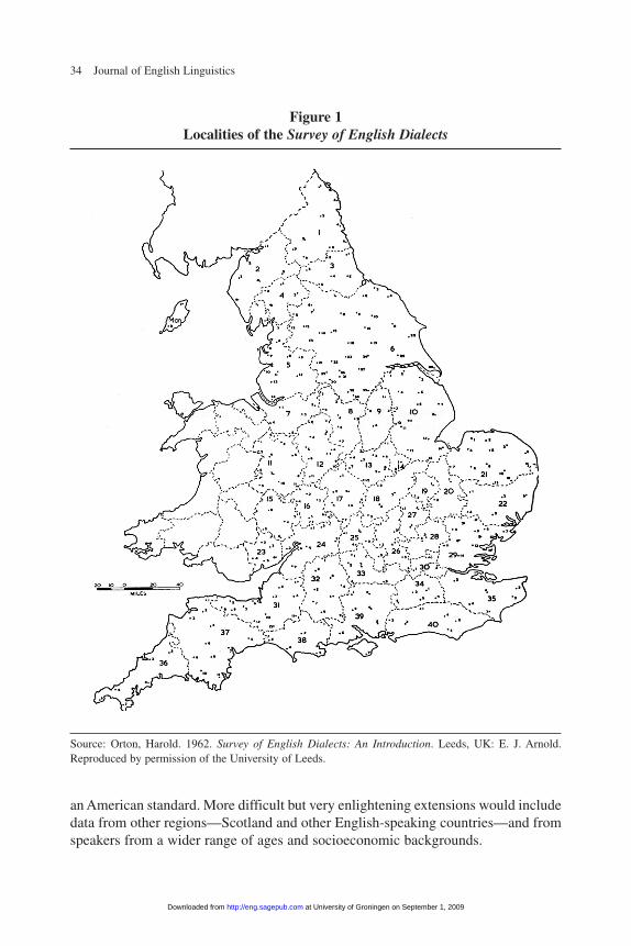
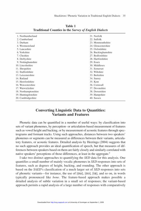
The SED responses were recorded impressionistically, using the 1951 revision ofthe International Phonetic Alphabet.6 The SED material is presented by locality, witha county name and number—for example, Northumberland 1—as illustrated infigure 1 and table 1. Geographic coordinates for each locality in the SED are takenfrom the United Kingdom’s Ordnance Survey website.7 All the results from a givenlocality are presented together, making it impossible to distinguish the responses ofindividual informants. The responses in the SED thus represent an aggregated sam-ple of the speech habits of a particular locality rather than those of a particular indi-vidual and will be referred to accordingly. Where the SED presents more than oneform of a word for a locality, I select the first unless another form is specificallyreferred to as “older” or “preferred.”
In addition to data taken directly from the SED, I take derived data fromAnderson’s Structural Atlas of the English Dialects (1987) or SAED, which presentsa series of more than 100 maps showing the geographic distribution and frequencyof occurrence of different phonetic variants in groups of words found in the SED,where all of the words in a given group include a segment that is posited to havetaken a single uniform pronunciation in an older form of the language—the “stan-dard” Middle English dialect of the Home Counties of southeastern England. Thegroups include all of the Middle English short and long vowels and diphthongs, andmost of the relatively few consonants that exhibit any variation in the Englishdialects. Although it is by no means complete or comprehensive, the data set reducesan enormous amount of phonetic information to a tractable form that makes possi-ble a rapid and wide-ranging analysis of phonetic variation in the traditional dialectsof England as they existed in the middle of the 20th century.9
To provide a somewhat broader perspective on the traditional English dialectsrecorded in the SED, I expand the data set to include the pronunciations of three ide-alized speakers: a speaker of the Middle English “standard” on which the SAEDclassification of localities’ responses is based; a speaker of mid-twentieth-centuryReceived Pronunciation; and a speaker of my own native speech pattern, the“Western Reserve” dialect of northern Ohio, which is the speech form chosen byAmerican radio broadcasters in the early 20th century as most closely representing
at University of Groningen on September 1, 2009 http://eng.sagepub.comDownloaded from
34 Journal of English Linguistics
an American standard. More difficult but very enlightening extensions would includedata from other regions—Scotland and other English-speaking countries—and fromspeakers from a wider range of ages and socioeconomic backgrounds.
Figure 1Localities of the Survey of English Dialects
Source: Orton, Harold. 1962. Survey of English Dialects: An Introduction. Leeds, UK: E. J. Arnold.Reproduced by permission of the University of Leeds.
at University of Groningen on September 1, 2009 http://eng.sagepub.comDownloaded from
Shackleton / Phonetic Variation in Traditional English Dialects 35
Converting Linguistic Data to Quantities:Variants and Features
Phonetic data can be quantified in a number of useful ways: by classification intosets of variant phonemes, by perception- or articulation-based measurement of featuressuch as vowel height and backing, or by measurement of acoustic features through spec-trograms and formant tracks. Using such approaches, distances between two speakers’phonemes or segments can be measured as differences between their variants, articula-tory features, or acoustic features. Detailed analysis by Heeringa (2004) suggests thatno such approach provides an ideal quantification of speech, but that measures of dif-ferences between speakers based on them are fairly closely and similarly correlated withnative speakers’ perceptions of those differences, at least in the aggregate.9
I take two distinct approaches to quantifying the SED data for this analysis. Onequantifies a small number of mainly vocalic phonemes in SED responses into sets offeatures, such as degrees of height, backing, and rounding. The other approach isbased on the SAED’s classification of a much larger set of SED responses into setsof phonetic variants—for instance, the use of [ou], [o«], [ia], and so on, in wordstypically pronounced like bone. The feature-based approach makes possible adetailed analysis of subtle variation in a small set of responses; the variant-basedapproach permits a rapid analysis of a large number of responses with comparatively
Table 1Traditional Counties in the Survey of English Dialects
1. Northumberland 21. Norfolk2. Cumberland 22. Suffolk3. Durham 23. Monmouthshire4. Westmoreland 24. Gloucestershire5. Lancashire 25. Oxfordshire6. Yorkshire 26. Buckinghamshire7. Cheshire 27. Bedfordshire8. Derbyshire 28. Hartfordshire9. Nottinghamshire 29. Essex
10. Lincolnshire 30. Middlesex11. Shropshire 31. Somerset12. Staffordshire 32. Wiltshire13. Leicestershire 33. Berkshire14. Rutland 34. Surrey15. Herefordshire 35. Kent16. Worcestershire 36. Cornwall17. Warwickshire 37. Devonshire18. Northamptonshire 38. Dorsetshire19. Huntingdonshire 39. Hampshire20. Cambridgeshire 40. Sussex
at University of Groningen on September 1, 2009 http://eng.sagepub.comDownloaded from

little effort. Comparing the results of the two approaches yields further understand-ing of their relative strengths and weaknesses and of dialect variation in general.Although comparison of strings of segments such as words or phrases would pro-vide further insight, the analysis considers only short segments in the interests ofeconomy.
On the whole, these approaches almost certainly considerably understate the fullextent of phonetic variation among the localities in the SED—the feature-basedapproach because it is based on such a small set of phonemes, and the variant-basedapproach because its classifications obscure a great deal of variation. That under-statement simplifies the use of various algorithms to uncover structure, but to suchan extent that a skeptic may reasonably wonder whether the results are not duemainly to the choice of classifications and words than to the use of quantitative tools.Despite their limitations, however, both data sets faithfully record a wide range ofvariation. Moreover, the sources of understatement do not appear likely to result inany other systematic bias in the measurement of dialect differences. As a result, thedistance measures, clusters, and factors uncovered in this study appear likely to berelatively robust to improvements in the measurement of true variation.
Feature-Based Approach: Quantification
The feature-based approach closely analyzes a set of 55 words shown in table A-1 in appendix A. The set includes at least one example of every short vowel, longvowel, and diphthong in “standard” Middle English, alone and followed by rhotics,as well as the variable consonants. The approach translates 122 segments (includingvowels, diphthongs, and consonants) into vectors of numerical values representing483 phonetic features. That translation—necessarily a somewhat arbitrary process—provides a numerical characterization of each segment that can be used to calculatea measure of perceptual or articulatory distance between segments.
According to the approach I adopt here—of my construction but similar to thesystem of Almeida and Braun (1986)—short and long vowels are represented as vec-tors of four values: 1.0 to 7.0 for height, 1.0 to 3.0 for the degree of backing, 1.0 to2.0 for rounding, and 0.5 to 2.0 for length. Thus, for instance, [a] takes values of[1.0, 0.0, 0.0, 1.0], while [u:] takes values of [7.0, 3.0, 2.0, 2.0]. (I ignore most dia-critics.) Diphthongs are represented by a vector of eight numbers; for example, [ou]and [o:«] would take values of [5.0, 3.0, 2.0, 1.0, 7.0, 3.0, 2.0, 1.0] and [5.0, 3.0, 2.0,2.0, 4.0, 2.0, 1.0, 0.5], respectively. For some types of analysis, I convert the valuesdescribing the second element of a diphthong to differences between the second ele-ment and the first. For the diphthongs above, for example, the values would be [5.0,3.0, 2.0, 1.0, 2.0, 0.0, 0.0, 0.0] and [5.0, 3.0, 2.0, 2.0, –1.0, –1.0, –1.0, –1.5]. Ifmonophthongs are assigned values of 0.0 for the second set of features, monoph-thongs and diphthongs can both be included in a square matrix, with the second set
36 Journal of English Linguistics
at University of Groningen on September 1, 2009 http://eng.sagepub.comDownloaded from
of features representing the characteristics of the glide. This second approach makespossible a novel analysis of variations in glide characteristics in the principal com-ponents analysis described below. Consonants are represented by a value represent-ing the presence or absence of the relevant distinctive feature; rhotics are representedby two values representing the place and manner of articulation.10 I also tabulate dataon whether multiple responses were recorded in a given locality and on the identityof the field worker.
Feature-Based Approach: Distribution and Correlations
Only 447 of the features have any variance; the remaining 36 are constant across alllocalities. That each word has its own history is underlined by the fact that the meansand standard deviations of vowel features are distributed more or less uniformly; that is,for any given feature—vowel height, for example—the mean value across localities forany given word is unique, and the mean values for all words show no distinctive patternat all. Even features of the vowels in words as similar as sun and butter have noticeablydifferent means and standard deviations. However, feature distributions reveal an impor-tant underlying pattern. For every feature, high standard deviations strongly tend to beassociated with middling average feature values, while low deviations are associatedwith extreme average values. For example, low or high vowels tend to have fairly uni-form distributions across speakers. A low (or high) vowel typically is low (or high) inmost localities, and so the standard deviation of its distribution tends to be low. In con-trast, vowels of medium height tend to have varied expressions across dialects and highstandard deviations in their distributions. The same observation holds for backing, round-ing, and length, but the pattern has different causes in different cases. For vowel heightand backing, it arises from the fact that the position of middling vowels such as [E] and[O] is quite variable—that is, that middling vowels tend to be rather unstable. In the caseof rounding and length, however, it is due mainly to the fact that features with averagevalues closer to the mean are simply those for which many localities uses a rounded orshort variant, while many others use an unrounded or long one.
Relatively few features are closely correlated. Only about 2 percent of all Pearsoncorrelations between features have an absolute value greater than 0.5, and only about15 percent are greater than 0.25. The typical feature will have a correlation withabsolute value of 0.5 or more with only a dozen other features. However, those aver-ages mask a great deal of variation in the degree of correlation among features.About a quarter of the features have no more than two correlations with absolutevalue greater than 0.5, but roughly another quarter have correlations that high with20 or more other features. On closer examination, the highly correlated features turnout to be composed largely of three classes—one composed of fricatives, which alltend to be voiced in the Southwest; another composed of features of second segmentsof diphthongs, which tend to develop inglides or downglides in the North and upglidesin the Southeast; and a third composed of rhotic features or, in the non-rhotic
Shackleton / Phonetic Variation in Traditional English Dialects 37
at University of Groningen on September 1, 2009 http://eng.sagepub.comDownloaded from
dialects, their replacements. Moreover, no feature values appear to be closely corre-lated with any particular field worker, suggesting that systematic field worker erroris relatively minor.
Variant-Based Approach: Quantification
In the variant-based approach, I use data from the SED and SAED to calculatelocalities’ frequencies of usage of groups of phonetic variants (mainly of vowels) ingroups of words believed to have had uniform pronunciations in “standard” MiddleEnglish. The variant-based data set summarizes over 400 responses in each locality,grouping them into 199 variants of 39 phonemes or combinations of phonemes.11
The full set of groups of variants is shown in table B-1 in appendix B; the words usedappear in the index of the SAED. (Throughout the rest of the presentation, I write theMiddle English form considered common—not to say ancestral—to the group as /x/and the variants recorded in the SED as [x].)
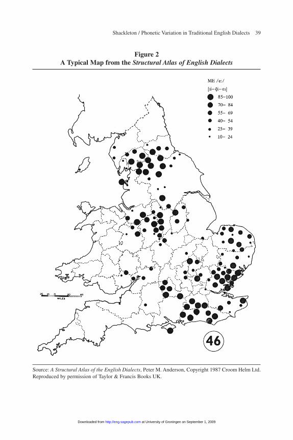
The typical map from the SAED shown in figure 2 illustrates strengths and weak-nesses of both the data and the approach. The map shows approximate frequenciesof use in SED localities of variants closely approximating [«i], [뺺i], or [Ii]—that is,rising diphthongs with a centered, center-front, or slightly higher than center-frontonset—in a set of 20 words, such as cheese and geese, believed to have been pro-nounced with /e:/ by speakers of “standard” Middle English.12 A closer examinationof the SED material reveals that the variants in question are not all used in eachregion: localities in the Southeast and East Anglia uniformly use [Ii]; those in theNorthwest Midlands tend to use [Ei] or [Ei¬ ], but occasionally [Ii]; and those in NorthYorkshire typically use [뺺 i] or [«i], but also occasionally [Ii]. In this case, then, theresponses can be classified further into three separate groups on the basis of differ-ences both geographical and linguistic. (In a few cases, I classify localities from geo-graphically separate regions as having “different” variants even though the variantsare actually the same, on the grounds that the variant is likely to have arisen inde-pendently in the two regions. For instance, localities in the North that use [i: ~ e:]in words with /ä:/ in Middle English are distinguished from those in the South andMidlands that use the same variant, since there is a large geographic gap between theregions in which the variant does not appear at all.)
I also translate the variants described in table B-1 into vectors of numerical val-ues representing features. In contrast to the first feature-based approach, I representshort monophthongs as a vector of three numbers representing height, backing, androunding; long monophthongs and diphthongs are represented by a vector of six val-ues. The treatment of consonants and rhotics follows the feature-based approach.Where a variant in table B-1 actually represents a range of distinguishable sounds,its characterization generally takes the mean value for each feature over the range ofsounds assigned to the specific variant in the SAED. As in the feature-basedapproach, I ignore most diacritics.
38 Journal of English Linguistics
at University of Groningen on September 1, 2009 http://eng.sagepub.comDownloaded from
Shackleton / Phonetic Variation in Traditional English Dialects 39
Figure 2A Typical Map from the Structural Atlas of English Dialects
Source: A Structural Atlas of the English Dialects, Peter M. Anderson, Copyright 1987 Croom Helm Ltd.Reproduced by permission of Taylor & Francis Books UK.
at University of Groningen on September 1, 2009 http://eng.sagepub.comDownloaded from

40 Journal of English Linguistics
The classification of words into groups imposes several limitations. It tends tounderstate the true extent of variation in several ways and, by precluding the pair-wise comparison of individual words or phonemes in words, limits the range ofapproaches that can be used to analyze that variation. A historical basis for groupingwords together is as compelling as any other approach, but the words may not in fact have been pronounced the same even in “standard” Middle English, in whichcase they may be inappropriately grouped even on the stated basis. In addition, spec-ified variants often comprise a range of distinguishable sounds—such as [«i], [ëºi],and [Ii] in the example above—thus masking a significant amount of variation.Similarly, even informants using traditional speech forms in a given locality mayhave substantially different usage that is masked by the presentation of the SEDmaterial by locality. Perhaps more importantly, two localities’ usage may differ con-siderably across a given group of words even if they have identical frequencies ofuse of each variant. In the extreme, one can imagine two localities using each of twovariants for 50 percent of the words, but using different variants for each word.Conversely, of course, the approach also may tend to overstate the true extent of vari-ation in some cases, as when two localities may use the same variant (for instance,[Ii] in the example above) but be classified as using different variants. Nevertheless,as mentioned above, the approach also has the advantage of allowing the rapid analy-sis of a large set of responses.
Variant-Based Approach: Distribution and Correlations
The full distribution of variants resembles the asymptotic hyperbolic (or A-curve)distribution discussed by Kretzschmar and Tamasi (2002) as being common todialect data: a small set of the variants in the data set accounts for most usage, whilethe majority has relatively limited distributions. The average variant is used in about20 percent of all localities, but 29 variants (about 15 percent of the total) are used in50 percent or more of all localities, while 73 (about 36 percent) are used in 5 percentor fewer. Ignoring variations in the frequency of occurrence of different phonemes,25 variants account for nearly half of all usage across all phonemes, while the leastcommon 115 variants account for only 10 percent.
Most variants have a relatively unique distribution among and frequency of usewithin SED localities. The distributions of variants may overlap a great deal—eventhe distributions of variants of the same phoneme—but they rarely entirely coincide.This can be seen most clearly in the Pearson correlations between variants. Onlyabout 3 percent of all the Pearson correlations between variants are greater than 0.5,and only about 11 percent are greater than 0.25. Those values imply that the typicalvariant will have a correlation of 0.5 or more with only 5 or 6 other variants and acorrelation of 0.25 or more with only about 20 of them. However, those averagesmask a great deal of variation in the degree of correlation among variants. Most vari-ants have very few large correlations with others: 53 variants have no correlations as
at University of Groningen on September 1, 2009 http://eng.sagepub.comDownloaded from
large as 0.5, and 95 variants have 3 or fewer. In contrast, 25 variants have 15 or morecorrelations of 0.5 or greater, and 35 variants have 12 or more. Interestingly, most ofthe variants with a large number of large correlations are found either in the farSouthwest or in the far North of England. That finding suggests that those tworegions tend to have relatively distinctive speech forms with numbers of features thatregularly co-occur in them, exemplified, for instance, by the very similar geographicdistributions of voiced fricatives in the Southwest.
With the exception of the extensive correlation of a relatively small group of vari-ants, the typically low levels of correlation among variants provide strong evidencethat most variants do not tend to co-occur very regularly with many others. Thatobservation, in turn, implies that localities in the SED may share specific variants incommon but are unlikely to share overall patterns of usage, and provides support forthe view of dialect variation as a largely continuous phenomenon. Neither do anyvariants correlate closely with field worker identity.
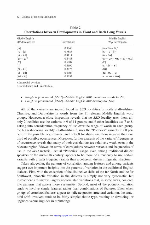
At the same time, the correlations among variants provide a number of clues asto the extent of systematic structural variation among the speech varieties in SEDlocalities. The most obvious example is fricative voicing in the Southwest; but per-haps the most notable instance is the set of positive correlations between paralleldevelopments in the Middle English front and back low long vowels shown intable 2. In much of the North of England, the vowels tend to merge with great reg-ularity. In other parts of the North, they both tend to develop inglides. In parts ofthe North Midlands, they are simply raised, and the degree of raising tends to becorrelated. Finally, the vowels both develop upglides in most of the South, andwhere they do, the heights of the initial vowels in the resulting diphthongs tend tobe similar. The co-evolution of the low front and back vowels thus appears to be agenuinely structural development in the English dialects. Note, however, that inmost of those cases the correlations between parallel developments, while positive,are not especially large: the structural parallels appear to be at least partly sys-tematic in nature but may perhaps best be interpreted as statistical tendenciesrather than strict relations.
In other cases, the correlations among variants reveal some proposed dialectstructures to be largely chimerical. For example, the “Potteries” dialect of northStaffordshire and surrounding counties has been characterized by the following pro-nunciations:13
• Bait and bate are pronounced [bi:t]; that is, Middle English /a:/ and /ai/ develop to [i:].• Beat and beet are pronounced [bEit]—Middle English /E:/ and /e:/ develop to [Ei].• Boat is pronounced [bü:t] or [bY:t]—Middle English /O:1/ or /O:2/ develop to
[ü: ~ Y:].• Boot is pronounced [bEot]—Middle English /o:/ develops to [Eo].• Bout is pronounced [bait]—Middle English /u:/ develops to [ai].• Bite is pronounced [b :t]—Middle English /i:/ develops to [ :].
Shackleton / Phonetic Variation in Traditional English Dialects 41
a a
at University of Groningen on September 1, 2009 http://eng.sagepub.comDownloaded from
42 Journal of English Linguistics
• Bought is pronounced [bout]—Middle English /ou/ remains or reverts to [ou].• Caught is pronounced [koot]—Middle English /au/ develops to [oo].
All of the variants are indeed found in SED localities in north Staffordshire,Cheshire, and Derbyshire in words from the 11 relevant Middle English wordgroups. However, a close inspection reveals that no SED locality uses them all; only 2 localities use the variants in 9 of 11 groups, and 6 other localities use 7 or 8.Taking into consideration frequency of use over the range of words in each group,the highest-scoring locality, Staffordshire 3, uses the “Potteries” variants in 60 per-cent of the possible occurrences, and only 8 localities use them in more than onethird of possible occurrences. Moreover, further analysis of the variants’ frequenciesof occurrence reveals that many of their correlations are relatively weak, even in therelevant region. Viewed in terms of correlations between variants and frequencies ofuse in the SED material, actual “Potteries” usage, even among traditional dialectspeakers of the mid-20th century, appears to be more of a tendency to use certainvariants with greater frequency rather than a coherent, distinct linguistic structure.
Taken altogether, the patterns of correlation among features and among variantssuggest two important insights into the patterns of variation in the traditional Englishdialects. First, with the exception of the distinctive shifts of the far North and the farSouthwest, phonetic variation in the dialects is simply not very systematic, butinstead tends to involve largely uncorrelated variations that, in some areas, coalesceinto patterns that appear more systematic. Second, most of the phonetic variationtends to involve single features rather than combinations of features. Even whengroups of correlated features appear to indicate greater structural variation, the struc-tural shift involved tends to be fairly simple: rhotic type, voicing or devoicing, orupglides versus inglides in diphthongs.
Table 2Correlations between Developments in Front and Back Long Vowels
Middle English Middle English/a:/ develops to: Correlation: /O:1/ develops to:
[i«] 0.8940 [i« ~ e« ~ E«]a
[iE ~ jE] 0.7883 [iE ~ jE ~ ji]a
[ia ~ ea] 0.9114 [ia ~ ea]a
[e« ~ E«]b 0.6488 [u« ~ o« ~ Uu« ~ O« ~ o:«][e:] 0.5987 [o:][i:] 0.4690 [u: ~ ü: ~ Y:] [ei ~ e:i] 0.3075 [ou][Ei ~ E:i] 0.5003 [Ou ~ u ~ u][æi ~ ai] 0.5032 [«u ~ Uu ~ æu]
a. In medial position.b. In Yorkshire and Lincolnshire.
a
at University of Groningen on September 1, 2009 http://eng.sagepub.comDownloaded from

Shackleton / Phonetic Variation in Traditional English Dialects 43
Calculating Linguistic Distances
A variety of measures can be used to quantify the difference between specificusages of one speaker or locality and another and to aggregate large numbers of suchdifferences into a single quantity, although none of them should be taken as a perfectlyaccurate gauge. For variants, for example, distances between specific phonetic seg-ments can be taken as 0 for speakers with the same variant or 1 for speakers with dif-ferent variants. For feature-based characterizations of segments, distances can becalculated using such measures as Manhattan “city-block” distance or Euclidean dis-tance. (For instance, the Manhattan distance between [e] and [u] is 7.0; the Euclideandistance is 4.6.) Such measures can be converted to logarithms—in this case, 1.95 and1.53, respectively—on the argument that small differences have a relatively greaterperceptual distance and should be given greater weight relative to larger ones.
Any measure of distance between segments can be extended to whole words orutterances using the more complex Levenshtein distance, which is defined as the min-imum cost of changing one word or utterance into another by means of insertions,deletions, and substitutions of one segment for another.14 Levenshtein distance isextremely useful for comparing dialects, particularly those with extensive metathesis,but it requires the coding of entire words rather than individual segments. I thereforefocus on segment-based measures instead.
Segments
To calculate a linguistic distance between segments, I introduce a somewhat novelmeasure of Euclidean distance between the articulation-based numerical characteriza-tions of segment features. The variant-based and feature-based approaches differslightly. In the variant-based approach, the distance calculation is generally intendedto reflect the number of changes that have occurred since the variants diverged froman ancestral monophthong or diphthong, so that the approach taken depends on thenature of both descendant variants and that of the inferred ancestral vowel. If both vari-ants are of the same type, the distance calculation is straightforward. If one variant isshort and the other long or a diphthong, the distance is generally calculated over thecharacteristics of the short variant and the first element of the long variant plus 1.0 forthe lengthening or the diphthong’s additional element in the diphthong. For example,the difference between [e] and [i:] is 1.414—the square root of the sum of 1.0 for thedistance between [e] and [i] plus 1.0 for lengthening. Matters get more complicatedstill if some descendants of an ancestral short or long phoneme have developedinglides and others offglides, as for example with Old English [o:] developing to [i«]in some northern dialects and to [oi] in parts of West Yorkshire. In this case, I calcu-late the distance between the features of the second element of the first diphthong andthose of the first element of the second one, adding 2.0 for the addition of an inglidein the former and an upglide in the latter. I make analogous adjustments for othercomplex comparisons, such as between shortened and diphthongized descendants of a
at University of Groningen on September 1, 2009 http://eng.sagepub.comDownloaded from
44 Journal of English Linguistics
long ancestral vowel. I generally give a value of 1.0 to distances between variants of consonants (which usually involve voicing or devoicing) except in the case of thevarious rhotics, where I calculate a Euclidean distance between two-element vectorsrepresenting place and manner of articulation.
The feature-based approach differs from the variant-based approach in treating allmonophthongs as single segments with four variable features, with length as a featureranging in value from 0.5 to 2.0. I calculate the distance between a monophthong anda diphthong over the characteristics of the monophthong and the first element of thelong variant plus 1.0 for the difference between a monophthong and a diphthong; thedistance between diphthongs is a straightforward Euclidean distance calculation overall eight features, ignoring considerations of historical development. Consonants andrhotics are treated as described for the variant-based approach.
Aggregation
Researchers can use a variety of different approaches to aggregate differencesbetween localities’usages—whether based on perception, articulation, or acoustics—andto calculate aggregate distance measures, with no approach likely to yield a perfect mea-sure. The present analysis aggregates feature-based Euclidean distances by taking theaverage distance over all 122 segments in the data set. An aggregate measure of 1.0 thusimplies that on average, two localities’ phonemes in this set of segments differ about asmuch as do [e] and [E] or [o] and [O]. Note that the aggregation does not take intoaccount the many segments that are unvarying across English localities. In that sense, theaggregation procedure greatly exaggerates the “true” degree of distance among localities.
The variant-based approach is generally similar, except for adjustments needed toaccommodate localities’ varying frequencies of use of several different variants. Inmany cases, localities may share some variants in common but not others, but by con-struction the data obscure the extent of word-by-word overlap. Localities with thesame frequencies of use of particular variants may or may not use them in the samewords. Since there is no way to determine the degree of overlap between them short ofcomparing them word by word, the analysis simplifies the process by assuming thatshared frequencies of a given variant correspond to shared pronunciations in specificwords (over which the localities have zero linguistic distance), and distributes theremainder uniformly among remaining variants and calculating distances accordingly.
Table 3 shows a simple example in which two speakers each occasionally use allthree variants over a given set of words (by assumption, only one variant per word),but with different frequencies of use. For the calculation of linguistic distance, theyare assumed to share pronunciations where their frequencies of use overlap; that is,the speakers are both assumed to use Variant 1 in 10 percent of the words, Variant 2in 10 percent, and Variant 3 in 30 percent. For the remaining 50 percent of words,Speaker 1 is assumed to use Variant 2, while Speaker 2 is assumed to use Variant 1in 30 percent and Variant 3 in 20 percent. The distance calculation between the twospeakers is thus 30 percent times 1.5 (the distance between Variants 1 and 2) plus 20
at University of Groningen on September 1, 2009 http://eng.sagepub.comDownloaded from
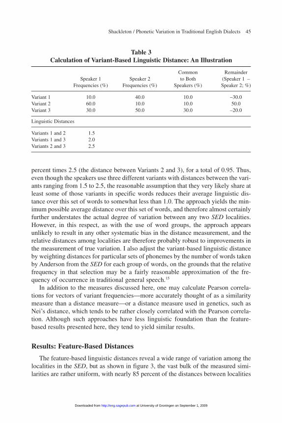
Shackleton / Phonetic Variation in Traditional English Dialects 45
percent times 2.5 (the distance between Variants 2 and 3), for a total of 0.95. Thus,even though the speakers use three different variants with distances between the vari-ants ranging from 1.5 to 2.5, the reasonable assumption that they very likely share atleast some of those variants in specific words reduces their average linguistic dis-tance over this set of words to somewhat less than 1.0. The approach yields the min-imum possible average distance over this set of words, and therefore almost certainlyfurther understates the actual degree of variation between any two SED localities.However, in this respect, as with the use of word groups, the approach appearsunlikely to result in any other systematic bias in the distance measurement, and therelative distances among localities are therefore probably robust to improvements inthe measurement of true variation. I also adjust the variant-based linguistic distanceby weighting distances for particular sets of phonemes by the number of words takenby Anderson from the SED for each group of words, on the grounds that the relativefrequency in that selection may be a fairly reasonable approximation of the fre-quency of occurrence in traditional general speech.15
In addition to the measures discussed here, one may calculate Pearson correla-tions for vectors of variant frequencies—more accurately thought of as a similaritymeasure than a distance measure—or a distance measure used in genetics, such asNei’s distance, which tends to be rather closely correlated with the Pearson correla-tion. Although such approaches have less linguistic foundation than the feature-based results presented here, they tend to yield similar results.
Results: Feature-Based Distances
The feature-based linguistic distances reveal a wide range of variation among thelocalities in the SED, but as shown in figure 3, the vast bulk of the measured simi-larities are rather uniform, with nearly 85 percent of the distances between localities
Table 3Calculation of Variant-Based Linguistic Distance: An Illustration
Common Remainder Speaker 1 Speaker 2 to Both (Speaker 1 –
Frequencies (%) Frequencies (%) Speakers (%) Speaker 2; %)
Variant 1 10.0 40.0 10.0 –30.0Variant 2 60.0 10.0 10.0 50.0Variant 3 30.0 50.0 30.0 –20.0
Linguistic Distances
Variants 1 and 2 1.5Variants 1 and 3 2.0Variants 2 and 3 2.5
at University of Groningen on September 1, 2009 http://eng.sagepub.comDownloaded from

46 Journal of English Linguistics
falling between 0.7 and 1.4. The average distance across all localities is about 1.1.(To put those values in perspective, consider that the maximum distance betweenshort vowels is about 7.3 and between long vowels or diphthongs is about 10.4, andthe distance between two randomly chosen vowels or diphthongs—or between tworandomly selected vectors of vowels—is thus likely to be around 4.4.) Relatively fewlocalities are radically different from each other, with the largest distances of nearly1.8 pointing to differences between Cumberland 1 on the Scottish border and anumber of localities in East Anglia and the Southwest. Nevertheless, even thoughneighboring localities are occasionally very similar in their speech forms—thesmallest distance points to a pair of localities in Somerset that are very nearly iden-tical in their speech—similarity appears to be the exception rather than the rule evenat relatively short geographic distances. Only about 2 percent of the distances areless than 0.5, implying that the typical locality will be that similar to no more than6 or 7 other localities. Thus, there are relatively few localities that are extremely sim-ilar in their speech but also relatively few (mainly those in Northumberland andDevonshire) that are quite different from the rest of England.
Localities have quite diverse patterns of close similarity. Some localities—mainlythose centered in broad regions with relatively uniform speech patterns, such as
0.0
0.5
1.0
1.5
2.0
2.5
0% 10% 20% 30% 40% 50% 60% 70% 80% 90% 100%
Feature-Based Variant-Based
Figure 3Distribution of Linguistic Distances
at University of Groningen on September 1, 2009 http://eng.sagepub.comDownloaded from
North Yorkshire, Leicestershire, and western Essex—have linguistic distances of lessthan 0.5 with as many as 25 other localities. In contrast, nearly 40 localities, whichgenerally appear to be either genuine outliers such as Cumberland 1 on the Scottishborder or in transition zones between regions of relative uniformity (Worcestershire1, Herefordshire 7, Hertfordshire 3, Oxfordshire 2, and Northamptonshire 5 beingnotable examples), have no feature-based distances of less than 0.5.
The distance measures are fairly closely correlated with geographic distance,with a Pearson correlation of 0.70—a strong indication that geographic separationhas played an important role in the differentiation of the traditional English dialects.One consequence of this fact is that localities in the middle of the country—localitiesthat often tend to have relatively large distances with neighboring localities becausethey are in or near a major transition zone between North and South—also tend tohave more in common with localities at both ends of the country than do localitiesat the ends with each other. Most of the localities with the lowest average distanceswith all other localities, ranging just above 0.9, are in the Midlands. In contrast, mostof the localities that are relatively distinctive from all other localities are in the FarNorth or the Southwest, with Cumberland 1 having the highest average of over 1.4.Standard deviations of distances tend to be highest for localities in the Southwest,suggesting that those localities tend to have a wide range of distances with otherlocalities, while skewness tends to be highest for localities in both the Far North andthe Southwest.16
Feature-based linguistic distances provide another prism through which to view the“Potteries” dialect region, which remains as indistinct as it was when analyzed in termsof variants. If we calculate linguistic distances between idealized “Potteries” pronun-ciations and SED responses for words from the relevant groups—gate, meat, cheese,white, loaf, moon, house, daisy, daughter, and snow—we find that localities aroundnorth Staffordshire have the smallest distances from the ideal, but that even the local-ities with the smallest distances—most of them slightly north of Staffordshire inDerbyshire, Cheshire, and Lancashire—have distances that are about 40 percent aslarge as the largest distances.
Data on the occurrence of multiple responses for features yield no strong patterns.On average, about 11 percent of localities provide multiple responses to a given word,but the frequency varies by word from 0 percent to over 60 percent. No obvious geo-graphic pattern emerges, although localities in three regions—the Thames Valley,Leicestershire, and East Yorkshire—appear to have the lowest frequencies of multipleresponses, suggesting that they are areas of relatively uniform speech.
Results: Variant-Based Distances
As shown in figure 3, the variant-based measure is more widely distributed com-pared with the feature-based distance, with smaller low values and larger high val-ues. (The source of that difference is not obvious, but I speculate that it is related to
Shackleton / Phonetic Variation in Traditional English Dialects 47
at University of Groningen on September 1, 2009 http://eng.sagepub.comDownloaded from
the much larger range of responses used in the variant-based analysis and the loweremphasis placed on differences in rhoticity.) Nevertheless, the feature-based andvariant-based linguistic distances are closely correlated, with a Pearson correlationof 0.817, and quite similar in patterns of similarity, difference, and correlation withdistance. Several broad regions appear to have relatively uniform speech patternsreflected in large numbers of relatively small linguistic distances, while localities inother regions have much higher shortest distances. Largely the same set of distinc-tively different localities, as in the feature-based analysis, appears to lie in transitionzones between regions of relative uniformity. The localities with the lowest averagevariant-based distances with all other localities are nearly all from the Midlands,while those with the highest average distances are nearly all from the Far North orthe Southwest. Patterns of standard deviations and skewness are also similar to thoseuncovered using the feature-based approach.
Middle English, Received Pronunciation,Western Reserve, and the SED
Comparison of linguistic distances between the SED localities and the three outliers—Middle English, Received Pronunciation, and Western Reserve—also yieldsseveral useful insights. As might be expected, no locality has speech patterns that arevery similar to Middle English. The mean average feature-based linguistic distance is about 1.7; the smallest is just under 1.3, and the largest is just under 1.9. For the variant-based distances, those values are nearly 1.8, just under 1.4, and over 2.6. Noclear geographic pattern of similarity emerges, except that localities in the Southwestare consistently the least similar to the Middle English standard. Otherwise, a band ofrather uniform dissimilarity with Middle English runs from the Upper North to thesoutheastern coast. Thus, the diachronic distance of roughly six centuries between the“standard” Middle English of southeastern England and the mid-20th-century tradi-tional dialects is, on average, about 45 percent to 50 percent greater than the averagesynchronic distance between the traditional dialects. Although the evidence may be tooslim to support the weight of the proposition, it may be appropriate to infer that speak-ers of traditional English dialects in the mid-20th century typically differed as much intheir speech as speakers in a given locality separated by roughly four centuries of time,and those with the greatest linguistic distances differed as much as speakers separatedby roughly seven to nine centuries.
Received Pronunciation has an average linguistic distance from SED localities that isroughly the same as the overall average—slightly higher for the feature-based distanceand slightly lower for the variant-based distance. It tends to have its lowest feature-baseddistances with eastern and East Midlands localities, particularly with those inCambridgeshire. It has its lowest variant-based distances with a somewhat more diversegroup of localities near the Home Counties—Huntingdonshire, Buckinghamshire, and
48 Journal of English Linguistics
at University of Groningen on September 1, 2009 http://eng.sagepub.comDownloaded from
Hertfordshire in particular—but also with various other localities in Herefordshire,Monmouthshire, and Norfolk. Those patterns may reflect a historical origin of ReceivedPronunciation in the Home Counties, but it may equally well reflect variations in theextent to which informants in SED localities used elements from the standard in theirspeech. In the absence of a compelling method of distinguishing between those two pos-sibilities, the data do not appear to provide a great deal of insight into the regional sourcesof Received Pronunciation, except of course that it does not come from Oxford.
Western Reserve has an average feature-based distance from the SED localities ofabout 1.25 and an average variant-based distance of roughly 1.31, consistent with atime distance of four to four-and-a-half centuries. Even considering only the south-ern half of England, from which most of the early settlers who influenced the devel-opment of American speech emigrated, Western Reserve has average distancesconsistent with a time distance of about three-and-a-half to four centuries—noticeablylarger than the time span from even the earliest English settlements in America to themid-20th century.17 Although Western Reserve’s feature-based distances are clearlylowest for localities in the Southwest and particularly in Somerset, in part becauseof their shared rhoticity, its variant-based distances are generally lowest for locali-ties spread through southern England from Shropshire to Kent. Western Reserve’slowest feature-based distance, 0.79 with Somerset 1, makes it more similar to thatlocality than all but 50 English localities—more similar, in fact, than some localitiesin neighboring counties—and places it rather squarely in the southwestern family ofdialects.
Perhaps a more revealing insight is that Received Pronunciation and WesternReserve are in many respects quite similar. Although their feature-based distance israther significant (0.99), they have a variant-based distance of roughly 0.53, makingthem more similar to each other by that measure than they are to any of the SEDlocalities, despite the non-rhotic nature of Received Pronunciation and the stronglyrhotic nature of Western Reserve. Closer examination reveals that the difference indistance measures is accounted for in very large part by the feature-based measure’sgreater weighting of differences in rhoticity.18 Nonetheless, even by that measure,Western Reserve’s distance from Received Pronunciation is only about 25 percentgreater than its closest distances, making the American variety closer to the Englishstandard than it is to all but 32 localities. Conversely, about 90 localities are closerto Received Pronunciation than is Western Reserve. The variant-based distanceimplies a time distance between the English and American “standards” of roughlytwo centuries, consistent with a separation around the time of the AmericanRevolution; but the feature-based distance implies a much greater time distance.Taken together, those findings seem to suggest that the development of an American“standard” may have been fairly strongly influenced by English norms, but that dis-tance measures at their current state of development provide only very rough gaugesfor the comparison of synchronic and diachronic differences.
Shackleton / Phonetic Variation in Traditional English Dialects 49
at University of Groningen on September 1, 2009 http://eng.sagepub.comDownloaded from
50 Journal of English Linguistics
Grouping Localities: Cluster Analysis and Multidimensional Scaling
Cluster analytic techniques are algorithms that divide the observations in a data set into classes, or clusters, based on relationships within the data—generally somemeasure of distance or difference between observations.19 Clustering can thus be saidto simplify the data by reducing the differences among observations to a relativelysmall set of relationships within and among clusters. I use clustering methods here toclassify localities into groups whose speech is relatively similar, as gauged by the dis-tance measures discussed above. Clustering techniques include non-hierarchicalmethods, in which the data are divided into an arbitrary number of groups and eachobservation is assigned to a particular group, and hierarchical methods, in whichgroups may be divided into subgroups. Non-hierarchical methods exclude any relationamong clusters, while hierarchical methods allow subclusters to be more or lessclosely related as members of larger clusters. “Divisive” hierarchical methods divideand subdivide a data set into subsets on the basis of distances between data points untilsome predetermined limit is reached; “agglomerative” hierarchical methods start witheach observation as a separate cluster, join the most similar ones, and continue to jointhe resulting clusters until all clusters have been united. Hierarchical methods can beused to produce phenograms: figures that resemble trees, in which the length and dis-tribution of the branches represent the degree of similarity among observations.
There is no perfect clustering technique, and different clustering techniques canproduce markedly different classifications, with the efficacy of any given techniquein correctly classifying observations depending in part on the nature of the data.20
One approach that tests the robustness of the results is to use a number of differentclustering techniques and distance measures, and to introduce perturbations into thedata to test whether such “noise” noticeably affects the classification of localities.Patterns that consistently emerge under different approaches and noisy data arelikely to reflect underlying patterns in the data.
For the feature-based approach, I apply seven different hierarchical methods tothe linguistic distance measures: Ward’s Method, Weighted Group Average orUnweighted Pair Group Method with Arithmetic Mean (UPGMA), UnweightedGroup Average, Single Linkage or Nearest Neighbor, Complete Linkage or FurthestNeighbor, Weighted Centroid, and Unweighted Centroid. For the variant-based dis-tance measures, I apply the same hierarchical methods to four different distancemeasures: Pearson correlation, Nei’s distance, and unweighted and weighted lin-guistic distance. For each method and distance measure, the clustering is carried out100 times with random perturbations to the data, all using the Rug/L04 softwaredeveloped by Peter Kleiweg.21
Geneticists use similar methods to infer relatedness among distinct populations,using data on the frequency of occurrence of different genetic variants in different
at University of Groningen on September 1, 2009 http://eng.sagepub.comDownloaded from
populations to calculate estimates of genetic distance such as Nei’s distance. Oneparticularly useful approach is to calculate a family tree that minimizes the squarederrors between the genetic distances between each pair of observations and the dis-tances between them along the branches of the estimated tree. (Other approachesused in genetics are generally less appropriate to distance data.) Here I apply twosuch estimations, called Kitsch and Fitch, to the variant-based measures of linguisticdistance, using programs from the Phylogeny Inference Package (PHYLIP v. 3.65)developed by Joseph Felsenstein.22
Multidimensional Scaling
Multidimensional scaling (MDS) refers to a set of mathematical techniques thatreduce the variation in a data set to a manageably small arbitrary number of dimen-sions, allowing the user to uncover fundamental relationships in the data.23 As clusteranalysis may simplify data by reducing variability to a relatively small set of clusters,multidimensional scaling simplifies the interrelationships in the data by reducing asmuch of the variation as possible to a relatively small number of dimensions.
MDS techniques are similar to the principal components techniques describedbelow, but involve weaker assumptions about the data. The techniques can be appliedto any measure of distance or difference between observations in the data set, and theycan be used to develop two- or three-dimensional maps in which distances betweenpoints reflect differences among the observations. Here, I apply MDS to the full set ofresults of the cluster analyses described above, reducing the variation to a set of pointsin three dimensions that can be represented as colors on a standard map, again usingthe Rug/L04 software. The results reveal relatively clear dialect regions and transitionzones that appear to be robust to variations in the clustering approach and distancemeasure used.
Results
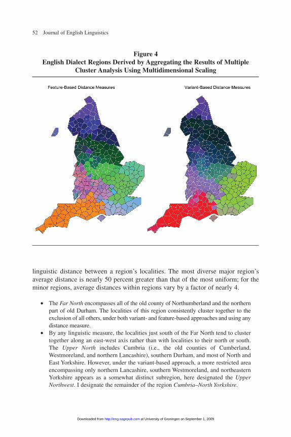
Different clustering methods tend to classify the speakers into a variety of differ-ent regional patterns. Nevertheless, taken as a whole the clustering methods producea rather clear picture of the traditional English dialect regions. Drawing on a rangeof algorithms and distance measures, and introducing multiple perturbations to testthe robustness of the results, the cluster analysis consistently yields the patterns ofclustering shown in the “honeycomb” maps in figure 4, one of which presents theoutput of a multidimensional scaling of the aggregated clustering results using all ofthe feature-based distance measures, and the other of which shows results using thevariant-based measures.24
The maps reveal a pattern of seven more or less distinct major regions androughly twice as many minor ones, appearing as differently shaded regions. Theregions vary quite a bit in the degree of uniformity, measured by the average
Shackleton / Phonetic Variation in Traditional English Dialects 51
at University of Groningen on September 1, 2009 http://eng.sagepub.comDownloaded from
52 Journal of English Linguistics
linguistic distance between a region’s localities. The most diverse major region’saverage distance is nearly 50 percent greater than that of the most uniform; for theminor regions, average distances within regions vary by a factor of nearly 4.
• The Far North encompasses all of the old county of Northumberland and the northernpart of old Durham. The localities of this region consistently cluster together to theexclusion of all others, under both variant- and feature-based approaches and using anydistance measure.
• By any linguistic measure, the localities just south of the Far North tend to clustertogether along an east-west axis rather than with localities to their north or south.The Upper North includes Cumbria (i.e., the old counties of Cumberland,Westmoreland, and northern Lancashire), southern Durham, and most of North andEast Yorkshire. However, under the variant-based approach, a more restricted areaencompassing only northern Lancashire, southern Westmoreland, and northeasternYorkshire appears as a somewhat distinct subregion, here designated the UpperNorthwest. I designate the remainder of the region Cumbria–North Yorkshire.
Figure 4English Dialect Regions Derived by Aggregating the Results of Multiple
Cluster Analysis Using Multidimensional Scaling
at University of Groningen on September 1, 2009 http://eng.sagepub.comDownloaded from

Shackleton / Phonetic Variation in Traditional English Dialects 53
• The localities in the Lower North also cluster along an east-west axis into a broad,linguistically relatively diverse region, including not only West and South Yorkshirebut also Lancashire (including Mersey and Greater Manchester), Cheshire,Derbyshire, Nottinghamshire, and most of Lincolnshire. Under any linguistic mea-sure, Lincolnshire in the east forms a distinct subregion that appears to bear affini-ties not only with the rest of the Lower North but also with the Upper North. Underthe feature-based measure, Cheshire-Derbyshire forms a quite distinct subregion aswell. Under the variant-based measure, I designate the Lower North excludingLincolnshire as the Lower Northwest.
• Linguistically speaking, the Central Midlands region is the most internally uniformof the broad regions. The Staffordshire subregion to the west, including nearly allof Staffordshire and the northern tip of Worcestershire, is rather more diverse, whilethe East Central Midlands, which includes the southeastern edge of Staffordshire,the northern half of Warwickshire, all of Leicestershire and Rutland, most ofNorthamptonshire, and most southerly section of Lincolnshire, is very uniform.
• The most linguistically diverse broad region is the Upper Southwest, even the sub-regions of which are more internally diverse than most of the major regions. A sub-region, designated the West Midlands, includes all of Shropshire, Hereford, andMonmouth, as well as most of Worcestershire and northwestern Gloucestershire. Asecond subregion, designated the Central South, includes the eastern edges ofWorcestershire and Gloucestershire, the southern half of Warwickshire, the south-western corner of Northamptonshire, all of Oxfordshire, most of Buckinghamshire,and western Bedfordshire.
• The Southeast, including all of East Anglia and the Home Counties, is more diversethan all other regions but the Upper Southwest, but its variation is more uniform fromlocality to locality. The region splits into three subregions: North Anglia, including allof Norfolk and most of Suffolk; the Central Southeast, including the southwestern cor-ner of Suffolk, Cambridgeshire, Huntingdonshire, most of Bedfordshire, Hertfordshire,Middlesex, Essex, and the areas of Kent and Surrey nearest to London; and theSoutheast Coast, which includes Berkshire, Sussex, most of Surrey and Kent, and theIsle of Wight.
• The Lower Southwest also splits into three regions, even though it is nearly as uniformas the Central Midlands despite including twice as many localities. The rather diverseCentral Southwest includes nearly all of Hampshire, all of Wiltshire and Dorsetshire,most of Somerset, and the southern half of Gloucestershire. Devonshire, which takesin all of that county as well as western Somerset and eastern Cornwall, is the most lin-guistically uniform subregion except for Lincolnshire, while Cornwall encompassesthe rest of that county.
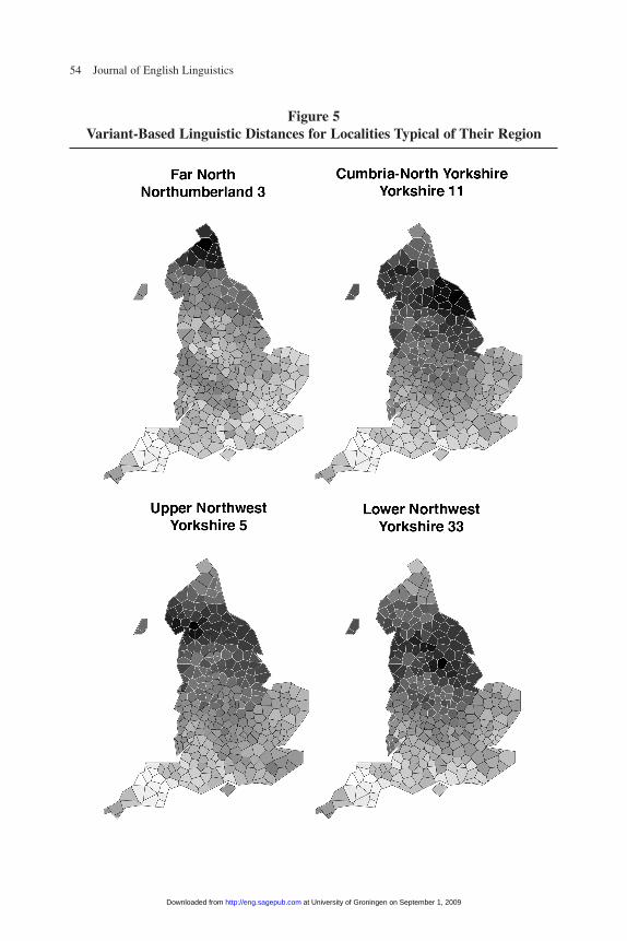
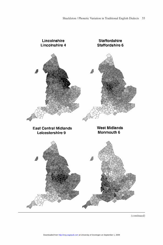
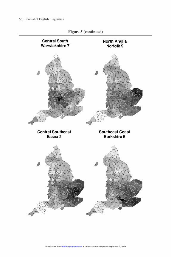
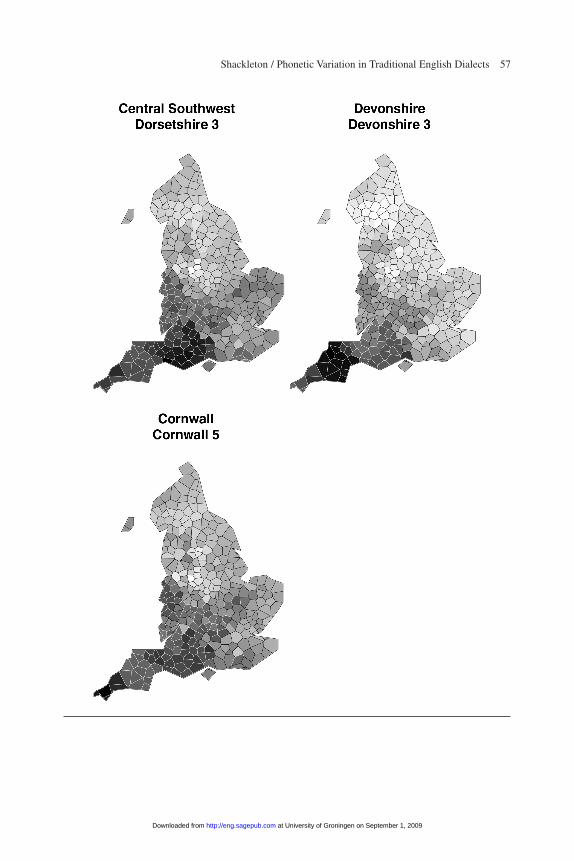
The maps in figure 5 illustrate the variant-based distances between the 15 most typ-ical regional localities and all of the other SED localities.25 Feature-based linguisticdistances between the most typical localities and the other localities in their regionsyield very similar patterns. Some localities are quite similar to all of the others in theirdesignated region, revealing a fairly large, relatively uniform dialect region. That pattern shows up quite clearly in the Far North, Lincolnshire, Leicestershire, and the
(text continues on 58)
at University of Groningen on September 1, 2009 http://eng.sagepub.comDownloaded from
54 Journal of English Linguistics
Figure 5Variant-Based Linguistic Distances for Localities Typical of Their Region
at University of Groningen on September 1, 2009 http://eng.sagepub.comDownloaded from
Shackleton / Phonetic Variation in Traditional English Dialects 55
(continued)
at University of Groningen on September 1, 2009 http://eng.sagepub.comDownloaded from
56 Journal of English Linguistics
Figure 5 (continued)
at University of Groningen on September 1, 2009 http://eng.sagepub.comDownloaded from
Shackleton / Phonetic Variation in Traditional English Dialects 57
at University of Groningen on September 1, 2009 http://eng.sagepub.comDownloaded from

58 Journal of English Linguistics
subregions of the Southwest. In other cases, the most typical localities do not appearto be strongly similar to many of the other speakers in their region at all—for instance,in the Lower Northwest, the West Midlands, and the Central South. Those regionsappear to be considerably less uniform in their speech patterns, and are perhaps betterthought of as transition zones than as distinct dialect regions. Other regions, notably inthe Upper North and the Southeast, are neither as uniform as Lincolnshire nor asdiverse as the Central South.
Under most approaches and measures, the most important boundary separates theSouth and Midlands, and the second most important separates the Southeast from theSouthwest and West Midlands; other important boundaries separate the Midlandsfrom the North, the Lower North from the Upper North, and the Upper North fromthe Far North. However, the application of multidimensional scaling to the aggre-gated results reveals subtle gradations within clusters as well as outliers within eachregion—for instance, Hampshire 4 and Somerset 1 in the Southwest, Bedford 1 andCambridgeshire 1 in the Southeast, and Oxfordshire 2 in the West Midlands. (Thefact that those localities take the colors of more distant regions does not necessarilyimply that they cluster with those regions; rather, they typically are transitionallocalities that have an unusual mix of variants from neighboring regions.) Someregions are very distinct, but others less so. In particular, the Central South, LowerNorthwest, and Lincolnshire subregions occasionally cluster into other regionsentirely, suggesting that the speech patterns in those regions have somewhat morediffuse affinities than most of the other regions. On the whole, however, the bound-aries are remarkably robust and clear, as are the transitional areas.
The regional clustering resulting from this approach finds corroboration in a sepa-rate approach involving average regional frequencies of variants and average regionalvalues of features. If one compares every locality’s frequencies of variant usage toregional average frequencies of variant usage, the usage patterns of the localities in thatregion are all nearly always more closely correlated with the region’s average usagethan are any other region’s localities. The same pattern holds for feature values: valuesof localities in a region are usually more closely correlated with that region’s averagefeature values than to those of any other region. (The exceptions tend to be preciselythose localities that appear as outliers in terms of linguistic distance within theirrespective regions.) For the Far North, for instance, every locality’s vector of variantfrequencies has a Pearson correlation of 0.86 or higher with the vector of averageregional frequencies in the Far North, while the next highest scoring locality has a cor-relation of 0.80. Moreover, in a majority of cases the locality with the highest correla-tion with the vector of average regional frequencies is also the “most typical” localityin the sense of having the lowest average distance with all the other localities in theregion. Those results reinforce the impression that the regional clustering is underlainby sets of linguistic characteristics in each region to which the localities in the respec-tive regions tend to gravitate.
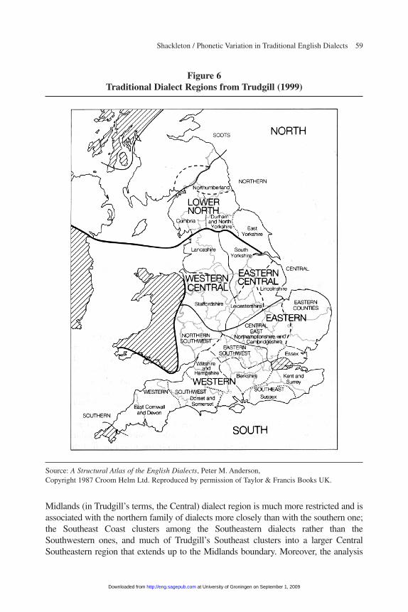
The dialect regions delineated here are very similar to those found in the dialect mapof Trudgill (1999), shown in figure 6, with only a few distinctive differences: the
at University of Groningen on September 1, 2009 http://eng.sagepub.comDownloaded from
Shackleton / Phonetic Variation in Traditional English Dialects 59
Midlands (in Trudgill’s terms, the Central) dialect region is much more restricted and isassociated with the northern family of dialects more closely than with the southern one;the Southeast Coast clusters among the Southeastern dialects rather than theSouthwestern ones, and much of Trudgill’s Southeast clusters into a larger CentralSoutheastern region that extends up to the Midlands boundary. Moreover, the analysis
Figure 6Traditional Dialect Regions from Trudgill (1999)
Source: A Structural Atlas of the English Dialects, Peter M. Anderson,Copyright 1987 Croom Helm Ltd. Reproduced by permission of Taylor & Francis Books UK.
at University of Groningen on September 1, 2009 http://eng.sagepub.comDownloaded from
60 Journal of English Linguistics
finds very little distinction between east and west in the northern dialect regions: parts ofCumberland consistently cluster with parts of eastern Yorkshire, and much of Lancashireconsistently clusters with Derbyshire and Nottinghamshire (though not Lincolnshire).
The delineation presented here also bears a strong resemblance to that described byEllis ([1889] 1968), except that Ellis places the Southeast Coast with the Southwestand Northamptonshire in the Southeast. It bears similarities to several maps presentedin some dialectometric studies using lexical and morphological variants in the SED,but differs noticeably from others. It resembles the “centers of gravity” described byHändler and Viereck (1997), exhibits a moderate degree of similarity with the clustersidentified by Goebl (1997) in a complete linkage analysis using several distance mea-sures over the same data, and is fairly similar to Thomas’s (1997) characterization aswell. However, the delineation is not very similar to that proposed by Goebl andSchiltz (1997) on the basis of localities’ number of shared features in that data, eventhough many of the relatively strong boundaries that they describe appear in figure 4;nor is it similar to the dialect division presented by Inoue and Fukushima (1997) on thebasis of a multivariate analysis of that data. It remains an open question whether or notan exactly analogous approach using lexical and morphological data would yieldessentially the same demarcation as the present study.
Phylogenetic Inference
Applied to the variant-based distance measures, the phylogenies produced by theKitsch and Fitch programs strongly support the delineation of dialect regions describedabove, including the major and minor boundaries and the various outliers. The onlynoticeable deviation is that the Midlands region tends to expand slightly north toinclude those localities in Cheshire and Derbyshire that are closest to Staffordshire. Inthe case of Fitch, the strongest boundary separates the Southeast from the rest ofEngland; in the case of Kitsch, it separates the North and South. Interestingly, and con-sistent with the modest variant-based linguistic distance between them, both ReceivedPronunciation and Western Reserve speech appear as a pair of fairly closely relatedoutliers—within the Southeast in the case of Kitsch, and separate from all the SEDlocalities in the case of Fitch.
Exploring Dialect Geography: Multiple Regression Analysis and Barrier Analysis
Multiple Regression Analysis
Multiple regression analysis quantifies the relationships between a variable of interest—a dependent variable—and a number of other independent variables, allow-ing for interaction among the latter.26 For instance, multiple regression can be applied
at University of Groningen on September 1, 2009 http://eng.sagepub.comDownloaded from

Shackleton / Phonetic Variation in Traditional English Dialects 61
to a set of measurements of a group of individuals’ weights, heights, waistlines, age,and gender to analyze how their weights vary with their other characteristics. (In thisexample, gender would be represented by a 0 for one gender and a 1 for the other; anindependent variable that takes this form is referred to as a “dummy” variable.)
I use regression analysis to test for a statistically significant relationship betweenthe various measures of linguistic distance between localities and the geographic dis-tance between them, using the Statistical Package for the Social Sciences (SPSS) forWindows Version 7.5 (SPSS 2006).27 However, by introducing dummy variables thatrepresent localities’ regional affiliations, distance regressions can be used to explorewhether differences among localities can be interpreted as being more or less whollya matter of geographic separation that has resulted in the gradual accumulation ofdifferences over generations, or whether those differences also vary systematicallyacross the dialect regions identified by cluster and phylogenetic analyses.
Distance Regressions
Table 4 shows the results of a regression of the variant-based linguistic distanceson the natural logs of geographic distances and on a set of intra- and interregionaldummy variables.28 Each of the 120 dummies takes a value of 1.0 only when twolocalities are from two specific regions. For example, the dummy variable Dummy,Regions 1 and 15 takes a value of 1.0 only when one locality is in the Far North andthe other is in Cornwall. As a result, the parameter that is estimated on this variableis based only on linguistic distances between localities in those two regions.
According to the adjusted R-square of the variant-based regression, geographicdistance and regional differences account for about 77 percent of the variation inmeasured linguistic distances. (Excluding the dummies, geographic distance aloneaccounts for about 50 percent.) All but four of the regional dummy variables are sta-tistically significant at the 0.99 level, an unusually strong result in any kind of cross-section regression; it points to speakers’ regional affiliations as an important sourceof their linguistic (dis)similarities. The value of the parameter for the geographic dis-tance variable indicates that ignoring regional affiliation (itself, however, partly afunction of geographic distance), 100 miles of distance between two localitiesincreases their linguistic distance by about 0.63 (0.137 times 4.605, the natural logof 100), and the average geographic distance of 129 miles should result in a linguis-tic distance of about 0.67, roughly 54 percent of the average linguistic distance.
The results of the feature-based regression (not shown) are quite similar: theadjusted R-square of the regression indicates that geographic distance and regionaldifferences account for about 80 percent of the variation in feature-based linguisticdistances; all but six of the regional dummy variables are highly significant; and geo-graphic distance parameter indicates that ignoring regional affiliation, the averagegeographic distance should result in a linguistic distance of about 0.68, about 62 per-cent of the average distance.
at University of Groningen on September 1, 2009 http://eng.sagepub.comDownloaded from
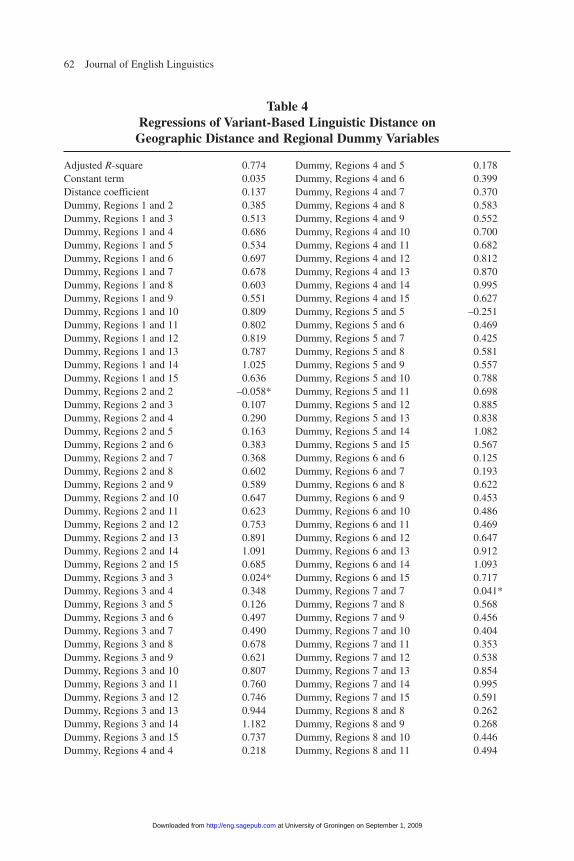
62 Journal of English Linguistics
Table 4Regressions of Variant-Based Linguistic Distance on
Geographic Distance and Regional Dummy Variables
Adjusted R-square 0.774Constant term 0.035Distance coefficient 0.137Dummy, Regions 1 and 2 0.385Dummy, Regions 1 and 3 0.513Dummy, Regions 1 and 4 0.686Dummy, Regions 1 and 5 0.534Dummy, Regions 1 and 6 0.697Dummy, Regions 1 and 7 0.678Dummy, Regions 1 and 8 0.603Dummy, Regions 1 and 9 0.551Dummy, Regions 1 and 10 0.809Dummy, Regions 1 and 11 0.802Dummy, Regions 1 and 12 0.819Dummy, Regions 1 and 13 0.787Dummy, Regions 1 and 14 1.025Dummy, Regions 1 and 15 0.636Dummy, Regions 2 and 2 –0.058*Dummy, Regions 2 and 3 0.107Dummy, Regions 2 and 4 0.290Dummy, Regions 2 and 5 0.163Dummy, Regions 2 and 6 0.383Dummy, Regions 2 and 7 0.368Dummy, Regions 2 and 8 0.602Dummy, Regions 2 and 9 0.589Dummy, Regions 2 and 10 0.647Dummy, Regions 2 and 11 0.623Dummy, Regions 2 and 12 0.753Dummy, Regions 2 and 13 0.891Dummy, Regions 2 and 14 1.091Dummy, Regions 2 and 15 0.685Dummy, Regions 3 and 3 0.024*Dummy, Regions 3 and 4 0.348Dummy, Regions 3 and 5 0.126Dummy, Regions 3 and 6 0.497Dummy, Regions 3 and 7 0.490Dummy, Regions 3 and 8 0.678Dummy, Regions 3 and 9 0.621Dummy, Regions 3 and 10 0.807Dummy, Regions 3 and 11 0.760Dummy, Regions 3 and 12 0.746Dummy, Regions 3 and 13 0.944Dummy, Regions 3 and 14 1.182Dummy, Regions 3 and 15 0.737Dummy, Regions 4 and 4 0.218
Dummy, Regions 4 and 5 0.178Dummy, Regions 4 and 6 0.399Dummy, Regions 4 and 7 0.370Dummy, Regions 4 and 8 0.583Dummy, Regions 4 and 9 0.552Dummy, Regions 4 and 10 0.700Dummy, Regions 4 and 11 0.682Dummy, Regions 4 and 12 0.812Dummy, Regions 4 and 13 0.870Dummy, Regions 4 and 14 0.995Dummy, Regions 4 and 15 0.627Dummy, Regions 5 and 5 –0.251Dummy, Regions 5 and 6 0.469Dummy, Regions 5 and 7 0.425Dummy, Regions 5 and 8 0.581Dummy, Regions 5 and 9 0.557Dummy, Regions 5 and 10 0.788Dummy, Regions 5 and 11 0.698Dummy, Regions 5 and 12 0.885Dummy, Regions 5 and 13 0.838Dummy, Regions 5 and 14 1.082Dummy, Regions 5 and 15 0.567Dummy, Regions 6 and 6 0.125Dummy, Regions 6 and 7 0.193Dummy, Regions 6 and 8 0.622Dummy, Regions 6 and 9 0.453Dummy, Regions 6 and 10 0.486Dummy, Regions 6 and 11 0.469Dummy, Regions 6 and 12 0.647Dummy, Regions 6 and 13 0.912Dummy, Regions 6 and 14 1.093Dummy, Regions 6 and 15 0.717Dummy, Regions 7 and 7 0.041*Dummy, Regions 7 and 8 0.568Dummy, Regions 7 and 9 0.456Dummy, Regions 7 and 10 0.404Dummy, Regions 7 and 11 0.353Dummy, Regions 7 and 12 0.538Dummy, Regions 7 and 13 0.854Dummy, Regions 7 and 14 0.995Dummy, Regions 7 and 15 0.591Dummy, Regions 8 and 8 0.262Dummy, Regions 8 and 9 0.268Dummy, Regions 8 and 10 0.446Dummy, Regions 8 and 11 0.494
at University of Groningen on September 1, 2009 http://eng.sagepub.comDownloaded from
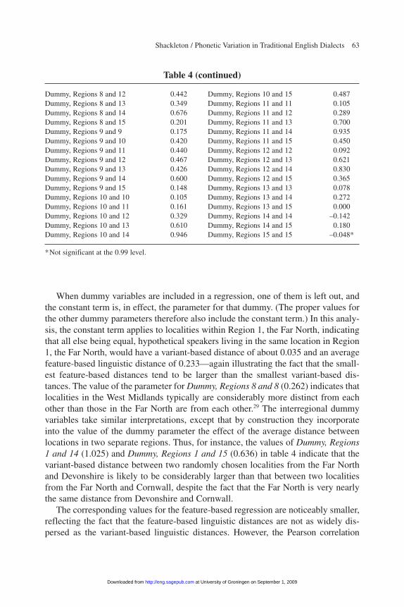
Shackleton / Phonetic Variation in Traditional English Dialects 63
When dummy variables are included in a regression, one of them is left out, andthe constant term is, in effect, the parameter for that dummy. (The proper values forthe other dummy parameters therefore also include the constant term.) In this analy-sis, the constant term applies to localities within Region 1, the Far North, indicatingthat all else being equal, hypothetical speakers living in the same location in Region1, the Far North, would have a variant-based distance of about 0.035 and an averagefeature-based linguistic distance of 0.233—again illustrating the fact that the small-est feature-based distances tend to be larger than the smallest variant-based dis-tances. The value of the parameter for Dummy, Regions 8 and 8 (0.262) indicates thatlocalities in the West Midlands typically are considerably more distinct from eachother than those in the Far North are from each other.29 The interregional dummyvariables take similar interpretations, except that by construction they incorporateinto the value of the dummy parameter the effect of the average distance betweenlocations in two separate regions. Thus, for instance, the values of Dummy, Regions1 and 14 (1.025) and Dummy, Regions 1 and 15 (0.636) in table 4 indicate that thevariant-based distance between two randomly chosen localities from the Far Northand Devonshire is likely to be considerably larger than that between two localitiesfrom the Far North and Cornwall, despite the fact that the Far North is very nearlythe same distance from Devonshire and Cornwall.
The corresponding values for the feature-based regression are noticeably smaller,reflecting the fact that the feature-based linguistic distances are not as widely dis-persed as the variant-based linguistic distances. However, the Pearson correlation
Table 4 (continued)
Dummy, Regions 8 and 12 0.442Dummy, Regions 8 and 13 0.349Dummy, Regions 8 and 14 0.676Dummy, Regions 8 and 15 0.201Dummy, Regions 9 and 9 0.175Dummy, Regions 9 and 10 0.420Dummy, Regions 9 and 11 0.440Dummy, Regions 9 and 12 0.467Dummy, Regions 9 and 13 0.426Dummy, Regions 9 and 14 0.600Dummy, Regions 9 and 15 0.148Dummy, Regions 10 and 10 0.105Dummy, Regions 10 and 11 0.161Dummy, Regions 10 and 12 0.329Dummy, Regions 10 and 13 0.610Dummy, Regions 10 and 14 0.946
Dummy, Regions 10 and 15 0.487Dummy, Regions 11 and 11 0.105Dummy, Regions 11 and 12 0.289Dummy, Regions 11 and 13 0.700Dummy, Regions 11 and 14 0.935Dummy, Regions 11 and 15 0.450Dummy, Regions 12 and 12 0.092Dummy, Regions 12 and 13 0.621Dummy, Regions 12 and 14 0.830Dummy, Regions 12 and 15 0.365Dummy, Regions 13 and 13 0.078Dummy, Regions 13 and 14 0.272Dummy, Regions 13 and 15 0.000Dummy, Regions 14 and 14 –0.142Dummy, Regions 14 and 15 0.180Dummy, Regions 15 and 15 –0.048*
*Not significant at the 0.99 level.
at University of Groningen on September 1, 2009 http://eng.sagepub.comDownloaded from
64 Journal of English Linguistics
between feature-based and variant-based dummies across equivalent regions is quitehigh (0.82) despite the fact that values for individual dummies are frequently very dif-ferent. That strong correlation—nearly as strong as the correlation between variant-based and feature-based linguistic distances—provides another indication that theregional variations uncovered in this analysis are quite robust to different characteri-zations of the phonetic data and likely reflect real patterns of dialect variation.
Table 5 illustrates the importance of regional speech differences, showing the per-centage difference between the average predicted variant-based linguistic distancesbetween localities in different regions, with and without regional dummies. Positivevalues indicate that localities in the relevant regions have greater than average speechdifferences, given their geographic separation; negative values point to smaller lin-guistic differences. For example, one of the largest values in table 5, 24.9 for interre-gional differences between Staffordshire and the bordering West Midlands, indicatesthat the dialect boundary between the two regions is a particularly significant one.Conversely, the quite negative values between North Anglia, the Central Southeast, andthe Southeast Coast point to relatively uniform speech across those three regions.Generally speaking, the largest values in the table apply to differences between dialectregions in the Midlands and Upper Southwest, suggesting that there is a broad centralregion of England of particularly great dialect diversity, perhaps because the conditionsfor interaction and influence among speakers are greater in a wide transition zonebetween the North, Southeast, and Southwest. Note also that the highest values amongintraregional dummies are for Staffordshire, the West Midlands, and the South Centralregion, all part of the large transition zone in the center of England; but the EastMidlands dummy takes a very low value, indicating that it, like its eastern neighborLincolnshire, is a much more uniform region linguistically than most of the regions to its west. The variant-based and feature-based values are generally similar, with aPearson correlation of 0.69.
The fact that the intraregional dummy variables include a distance component com-plicates the interpretation of their values and that of the geographic distance term aswell. Put simply, the effect of geographic distance on speech differences betweenregions is highly variable. Other non-geographic influences also affect linguistic dif-ferences over long distances; they are not quite as important as geographic distancealone, on average, but between some regions they can be at least as important, eitherenhancing or offsetting the effect of geographic distance on speech differences.
The regression results yield several important insights. The highly significant geo-graphic distance coefficients suggest that regional dialect diversity is closely tied togeographic separation and that such diversity is largely continuous. Distance aloneaccounts for at least half of phonetic variation in the traditional English dialects.However, differences in the magnitudes of the intraregional dummy variables point toregions of relative uniformity as well as regions of much greater diversity, controlling forgeographic distance. Moreover, the highly statistically significant dummy parameters
at University of Groningen on September 1, 2009 http://eng.sagepub.comDownloaded from
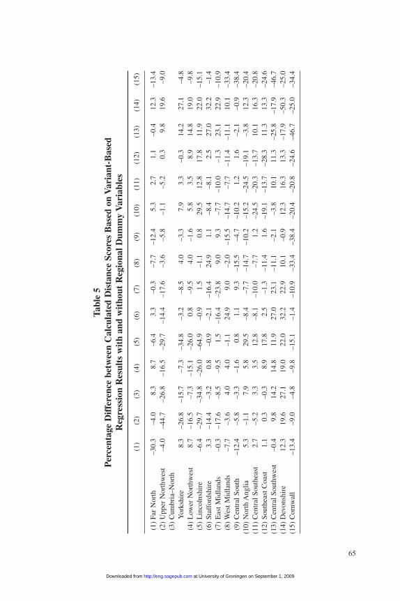
65
Tabl
e 5
Per
cent
age
Dif
fere
nce
betw
een
Cal
cula
ted
Dis
tanc
e Sc
ores
Bas
ed o
n V
aria
nt-B
ased
R
egre
ssio
n R
esul
ts w
ith
and
wit
hout
Reg
iona
l Dum
my
Var
iabl
es
(1)
(2)
(3)
(4)
(5)
(6)
(7)
(8)
(9)
(10)
(11)
(12)
(13)
(14)
(15)
(1)
Far
Nor
th–3
0.3
–4.0
8.3
8.7
–6.4
3.3
–0.3
–7.7
–12.
45.
32.
71.
1–0
.412
.3–1
3.4
(2)
Upp
er N
orth
wes
t–4
.0–4
4.7
–26.
8–1
6.5
–29.
7–1
4.4
–17.
6–3
.6–5
.8–1
.1–5
.20.
39.
819
.6–9
.0(3
) C
umbr
ia–N
orth
Y
orks
hire
8.3
–26.
8–1
5.7
–7.3
–34.
8–3
.2–8
.54.
0–3
.37.
93.
3–0
.314
.227
.1–4
.8(4
) L
ower
Nor
thw
est
8.7
–16.
5–7
.3–1
5.1
–26.
00.
8–9
.54.
0–1
.65.
83.
58.
914
.819
.0–9
.8(5
) L
inco
lnsh
ire
–6.4
–29.
7–3
4.8
–26.
0–6
4.9
–0.9
1.5
–1.1
0.8
29.5
12.8
17.8
11.9
22.0
–15.
1(6
) St
affo
rdsh
ire
3.3
–14.
4–3
.20.
8–0
.9–2
.1–1
6.4
24.9
1.1
–8.4
–8.1
2.5
27.0
32.2
–1.4
(7)
Eas
t Mid
land
s–0
.3–1
7.6
–8.5
–9.5
1.5
–16.
4–2
3.8
9.0
9.3
–7.7
–10.
0–1
.323
.122
.9–1
0.9
(8)
Wes
t Mid
land
s–7
.7–3
.64.
04.
0–1
.124
.99.
0–2
.0–1
5.5
–14.
7–7
.7–1
1.4
–11.
110
.1–3
3.4
(9)
Cen
tral
Sou
th–1
2.4
–5.8
–3.3
–1.6
0.8
1.1
9.3
–15.
5–4
.7–1
0.2
1.2
1.6
–2.1
–0.9
–38.
4(1
0) N
orth
Ang
lia5.
3–1
.17.
95.
829
.5–8
.4–7
.7–1
4.7
–10.
2–1
5.2
–24.
5–1
9.1
–3.8
12.3
–20.
4(1
1) C
entr
al S
outh
east
2.7
–5.2
3.3
3.5
12.8
–8.1
–10.
0–7
.71.
2–2
4.5
–20.
3–1
3.7
10.1
16.3
–20.
8(1
2) S
outh
east
Coa
st1.
10.
3–0
.38.
917
.82.
5–1
.3–1
1.4
1.6
–19.
1–1
3.7
–28.
311
.313
.3–2
4.6
(13)
Cen
tral
Sou
thw
est
–0.4
9.8
14.2
14.8
11.9
27.0
23.1
–11.
1–2
.1–3
.810
.111
.3–2
5.8
–17.
9–4
6.7
(14)
Dev
onsh
ire
12.3
19.6
27.1
19.0
22.0
32.2
22.9
10.1
–0.9
12.3
16.3
13.3
–17.
9–5
0.3
–25.
0(1
5) C
ornw
all
–13.
4–9
.0–4
.8–9
.8–1
5.1
–1.4
–10.
9–3
3.4
–38.
4–2
0.4
–20.
8–2
4.6
–46.
7–2
5.0
–34.
4
at University of Groningen on September 1, 2009 http://eng.sagepub.comDownloaded from
66 Journal of English Linguistics
indicate that systematic differences between regional speech forms account forroughly a quarter of the variation in the dialects.
Variant-Area Regressions
A regression of the number of variants in each region on the number of localitiesfurther reinforces the sense of varying degrees of regional uniformity. Biologists havelong noted a regular correspondence between (the log of) the number of species thatinhabit a geographic region and (the log of) its size—the species-area relationship.Consistent with the view that speech variants inhabit a speech region and are subjectto mutation and selection pressures analogous to those that affect species in the bios-phere, a similar pattern tends to obtain between the number of speech variants in useand the number of localities. In the present data set, there is a high degree of correla-tion between the number of variants and the number of localities in the 15 regionsdelineated by cluster and phylogenetic analysis; a log-log regression of the number ofvariants on the number of localities suggests that given the number of localities alreadyinterviewed, an interview in an additional locality in a region will typically increase thenumber of variants found in the region by about 1.3, and that such a relationshipaccounts for about two thirds of the variation in the number of variants by region.
Moreover, the errors or residuals in the variant-area regression provide useful infor-mation about the relative uniformity of speech in different regions. Those errors areparticularly positive in Lincolnshire, Cumbria–North Yorkshire, and the CentralSoutheast, while the most negative errors are for Staffordshire, the Central Southregion, and the Southeast Coast. Those errors indicate that the former group of regions(which are also regions in which linguistic distances are relatively small comparedwith geographic ones) tend to have lower diversity in terms of the number of variants,while the latter group (which also tend to have greater linguistic diversity over a givengeographic distance) tend to have greater diversity in terms of the number of variants.
Barrier Analysis
The importance of geography in determining the distribution of speech forms can befurther analyzed by examining the distribution of residuals or errors in regressions oflinguistic distance on geographic distance: a series of large positive errors generallyindicates an important dialect boundary that marks a relatively large number of linguis-tic changes over a short distance, whereas a series of large negative errors probably indicates unusually uniform speech over a relatively broad area. Monmonier (1973)developed a maximum difference algorithm that analyzes distance measures to mapimportant boundaries. An illuminating example of its use by Manni and Barrai (2001)tests the associations between dialect differences, gene frequencies, and the distributionof surnames in the Italian province of Ferrara. Applied to English dialect data,Monmonier’s algorithm may complement regression analysis in identifying important
at University of Groningen on September 1, 2009 http://eng.sagepub.comDownloaded from
Shackleton / Phonetic Variation in Traditional English Dialects 67
speech boundaries. The algorithm is implemented using the Barrier Version 2.2 soft-ware package developed by Manni, Guérard, and Heyer (2004).30
Applied to matrices of feature-based and variant-based linguistic distances,Monmonier’s algorithm produces broadly similar results that are, in each case, largelyconsistent with the regional classification developed above. (Applying the algorithm toresiduals of a regression of variant-based or feature-based distances on geographic dis-tances tends to yield similar patterns.) The algorithm identifies many of the sameregional boundaries as do the cluster and phylogenetic analyses, including thosebetween the Southeast and Southwest, the Upper Southwest and the Central Midlands,the Far North and Upper North, and the subregions of the Southeast, Upper Southwest,and Lower Southwest. The algorithm also identifies several other barriers withinregions: using either set of distance measures, it isolates areas of south Lancashire,Cheshire, and Derbyshire as distinctive subregions; and using one measure or the other,it isolates West Yorkshire, Devonshire, Somerset, or Essex. However, the algorithmtends not to find clear boundaries along the eastern English coast, between Yorkshireand Lincolnshire, Lincolnshire and the East Midlands, or East Midlands and theSoutheast.
In addition, roughly half of the boundaries the algorithm identifies isolate individuallocalities that are particularly distinct from their neighbors. A few of those lie well awayfrom any of the others, such as Cumberland 1 and Essex 7, and a few are in Hampshireon the boundary between the Lower Southwest and the Southeast Coast. However,pointing yet again to the region’s unusual linguistic diversity, the great majority of dis-tinctive localities are in or near the Upper Southwest, including Shropshire 2 and 5, sev-eral localities in Monmouth, Gloucestershire 4, Worcestershire 1 and 7, Oxfordshire 2and 3, Buckingham 6, and Hertfordshire 3.
Uncovering Linguistic Structure: Principal Components Analysis
Like cluster analysis and MDS, principal components analysis (PCA) reduces thenumber of dimensions in a data set, but it does so by finding groups of strongly corre-lated variables that are uncorrelated with the rest of the variables, and reducing them toa single “latent” variable—called a principal component, or PC—that is essentially alinear combination of the correlated variables.31 In effect, PCA clusters groups of vari-ables (in this case, feature values or variant frequencies) in a manner somewhat analo-gous to that in which cluster analysis distinguishes groups of observations (in this case,localities). PCA may thus allow a researcher to summarize the patterns of relationshipamong the variables as a smaller number of uncorrelated variables that contain most ofthe information in the data set.
Applied to a data set of linguistic features, PCA may isolate groups of variants or features that tend to occur together and that, with any luck, have a structural
at University of Groningen on September 1, 2009 http://eng.sagepub.comDownloaded from

68 Journal of English Linguistics
linguistic interpretation. Factor scores, which measure the strength of a particularprincipal component in the data for each locality, may reveal associations betweenthose linguistic structures and specific regions. In short, properly performed andinterpreted PCA may provide a relatively objective way of defining dialects anddialect regions. I use the Statistical Package for the Social Sciences (SPSS) forWindows Version 7.5 for the variant-based analysis and the current version ofSAS/STAT for the feature-based analysis.32
PCA uncovers sets of variables whose values are strongly positively or negativelycorrelated—that is, groups of variants that tend to occur together or that tend to occurseparately. (Variables that always occur separately are not independent; mathemati-cally speaking, independence, or orthogonality, implies that there is no pattern of co-occurrence at all. In visual terms, negative correlation places variants at opposite polesof a line, such as north and south, while independence places them at ninety degreesto each other on a perpendicular line—that is, north and east.) PCs therefore typicallyhave two poles: one pole will have large positive values for a group of variables thattend to be found together, and the other will have large negative values for anothergroup of variables that are also found together but never with the first group. As a ruleof thumb, researchers take into consideration only variables with scores of 0.32 andlarger in absolute value as part of a PC.
In the standard approach, each PC is uncorrelated with, or orthogonal to, all theothers. The first PC “extracts” or accounts for the maximum possible variance fromthe data set that can be accounted for by a single linear combination of variables; thesecond extracts the maximum possible amount of the remaining variance, and so on.Each variable is assigned a score in each PC, but will typically take a low value inall but one or at most a few PCs. A given observation, however, may have high factorscores for several quite different PCs.
Several variations on the standard PCA approach allow for the adjustment of PCs inways that simplify them, generally by placing more emphasis on the highest-scoringvariants (in technical terms, by “rotating” them to increase the loading on those vari-ables). Orthogonal rotations leave the PCs uncorrelated, whereas non-orthogonal rota-tions allow for some correlation between PCs. In the present study, orthogonal rotationtypically yields more clearly interpretable sets of variables than does standard PCA,especially when applied to variants rather than to features; and the groups of variablesthus identified appear also to be used by localities in more sharply defined regions. Forthe most part, however, non-orthogonal rotation does not appear to be warranted forthese data sets because non-orthogonal PCs, when rotated, prove to be largely uncor-related.
PCA yields a large number of PCs, raising the issue of how many to interpret asyielding useful information. Although there is no hard and fast rule in this regard, themost widely recommended approach is called the scree test, which recommendsretaining PCs that account for the greatest amount of variation up to the point at whichthe explained variation drops precipitously from one PC to the next, and disregardingPCs below the “break.”33 Applying PCA to the feature-based and variant-based data
at University of Groningen on September 1, 2009 http://eng.sagepub.comDownloaded from

Shackleton / Phonetic Variation in Traditional English Dialects 69
yields obvious breaks, but several of the PCs beyond the breaks are easily interpretablein linguistic terms and have factor scores that link them to geographically coherentregions that are similar, in many cases, to the regions delineated by the cluster analy-ses, suggesting that in some cases the scree test may be safely ignored.
Feature-Based Results
Because it allows for continuous variation in articulation, at least in the case ofvocalic features, the feature-based PC analysis yields PCs whose values may vary con-tinuously as a function of articulation.34 Only a handful of unrotated PCs yield clear,easily interpreted results in the feature-based approach. Consider the first unrotated PC,whose PC scores are presented in table 6 and whose factor scores appear in the first mapof figure 7, and which captures about 12 percent of total variation in the data. The firstPC clearly distinguishes southern, and particularly Southwestern, English features fromnorthern ones, with more central regions yielding intermediate factor scores. The highest-scoring features generally involve the raising or lengthening of some short vowels, thebacking and rounding of /a/ after /w/, and the lowering, backing, and unrounding of/u/—all general southern English innovations. Other features associated with theSouthwest also take relatively large values in the PC, including manner of rhoticity andfricative voicing. Southeastern L-vocalization also scores relatively strongly, andanother set of large values obtains for degrees of height, backing, and rounding in manyof the diphthongized Middle English long vowels. (Recall that the values describing thesecond element of a diphthong are converted to differences between the second elementand the first.) These values have a straightforward interpretation: upgliding variants like[ i ~ Oi] in night or [æi ~ ai] in gate will tend to yield relatively large positive scores,while long or ingliding variants like [i:] in night or [ia] in gate will yield low scores orlarge negative scores. The first PC is thus capturing the contrast between southernupglides and northern inglides or downglides, and is translating longer glides into largerPC scores. Note, however, that the first PC can only rather loosely be thought of as representing actual southern and northern speech patterns: many of the Southwesternfeatures to which it assigns large positive scores—fricative voicing and rhoticity in particular—are not found in the Southeast, and upgliding is generally muted in theSouthwest.
In contrast to the first PC, the second, which accounts for about 10 percent of thevariation and whose factor scores appear in the second map of figure 7, clearly dis-tinguishes the Southeast and Central Midlands regions from both the Southwest andthe North, assigning negative scores to the former and its strongest negative scoresto localities nearest London—precisely those localities in which upglides tend to bemost extended. While the PC does a good job of locating upgliding in the appropri-ate regions, however, it assigns positive scores not only to ingliding features in theNorth but also to rhotic and fricative features found in the Southwest. In this case, in
(text continues on p. 74)
a
at University of Groningen on September 1, 2009 http://eng.sagepub.comDownloaded from
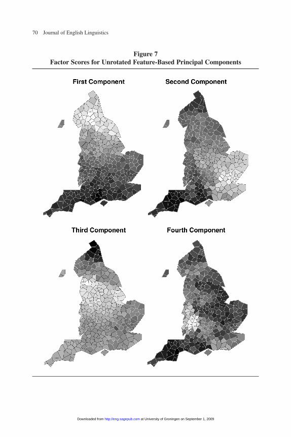
70 Journal of English Linguistics
Figure 7Factor Scores for Unrotated Feature-Based Principal Components
at University of Groningen on September 1, 2009 http://eng.sagepub.comDownloaded from
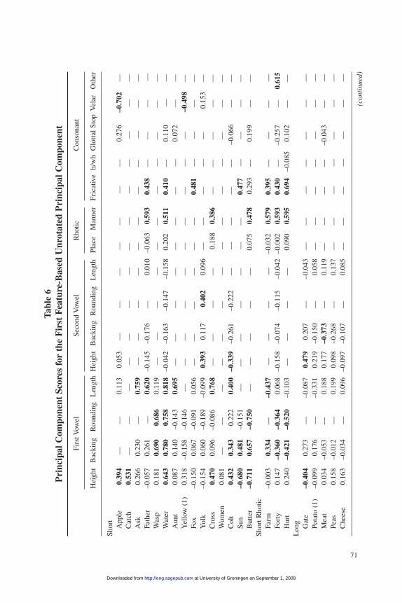
71
Tabl
e 6
Pri
ncip
al C
ompo
nent
Sco
res
for
the
Fir
st F
eatu
re-B
ased
Unr
otat
ed P
rinc
ipal
Com
pone
nt
Firs
t Vow
elSe
cond
Vow
elR
hotic
Con
sona
nt
Hei
ght
Bac
king
Rou
ndin
gL
engt
hH
eigh
tB
acki
ngR
ound
ing
Len
gth
Plac
eM
anne
rFr
icat
ive
h/w
hG
lotta
l Sto
pV
elar
Oth
er
Shor
tA
pple
0.39
4—
—0.
113
0.05
3—
——
——
——
0.27
6–0
.702
—C
atch
0.53
1—
——
——
——
——
——
——
—A
sk0.
266
0.23
0—
0.75
9—
——
——
——
——
——
Fath
er–0
.057
0.26
1—
0.62
0–0
.145
–0.1
76—
0.01
0–0
.063
0.59
30.
438
——
——
Was
p0.
181
0.69
00.
686
0.11
9—
——
——
——
——
——
Wat
er0.
643
0.78
00.
758
0.81
8–0
.042
–0.1
63–0
.147
–0.1
580.
202
0.51
10.
410
—0.
110
——
Aun
t0.
087
0.14
0–0
.143
0.69
5—
——
——
——
—0.
072
——
Yel
low
(1)
0.31
8–0
.158
–0.1
46—
——
——
——
——
—–0
.498
—Fo
x–0
.150
0.06
7–0
.091
0.05
6—
——
——
—0.
481
——
——
Yol
k–0
.154
0.06
0–0
.189
–0.0
990.
393
0.11
70.
402
0.09
6—
——
——
0.15
3—
Cro
ss0.
470
0.09
6–0
.086
0.76
8—
——
—0.
188
0.38
6—
——
——
Wom
en0.
081
——
——
——
——
——
——
——
Col
t0.
432
0.34
30.
222
0.40
0–0
.339
–0.2
61–0
.222
——
——
—–0
.066
——
Sun
–0.6
800.
481
–0.1
51—
——
——
——
0.47
7—
——
—B
utte
r–0
.711
0.65
7–0
.750
——
——
—0.
075
0.47
80.
293
—0.
199
——
Shor
t Rho
ticFa
rm–0
.003
0.33
4—
–0.4
37—
——
—–0
.032
0.57
90.
395
——
——
Fort
y0.
147
–0.3
60–0
.364
0.06
8–0
.158
–0.0
74–0
.115
–0.0
42–0
.002
0.59
30.
430
—–0
.257
—0.
615
Hur
t0.
240
–0.4
21–0
.520
–0.1
03—
——
—0.
090
0.59
50.
694
–0.0
850.
102
——
Lon
gG
ate
–0.4
040.
273
—–0
.087
0.47
90.
207
—–0
.043
——
——
——
—Po
tato
(1)
–0.0
990.
176
—–0
.331
0.21
9–0
.150
—0.
058
——
——
——
—M
eat
0.03
4–0
.053
—0.
188
0.17
7–0
.373
—0.
119
——
——
–0.0
43—
—Pe
as0.
158
–0.0
12—
0.19
90.
098
–0.2
68—
0.13
7—
——
——
——
Che
ese
0.16
3–0
.034
—0.
096
–0.0
97–0
.107
—0.
085
——
——
——
—
(con
tinu
ed)
at University of Groningen on September 1, 2009 http://eng.sagepub.comDownloaded from
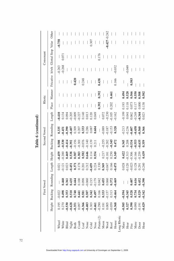
72
Tabl
e 6
(con
tinu
ed)
Firs
t Vow
elSe
cond
Vow
elR
hotic
Con
sona
nt
Hei
ght
Bac
king
Rou
ndin
gL
engt
hH
eigh
tB
acki
ngR
ound
ing
Len
gth
Plac
eM
anne
rFr
icat
ive
h/w
hG
lotta
l Sto
pV
elar
Oth
er
Whe
el0.
195
–0.0
22—
0.02
1–0
.459
0.50
80.
335
–0.4
10—
——
–0.2
63—
–0.7
58—
Whi
te0.
270
0.49
80.
460
–0.1
21–0
.200
–0.5
30–0
.451
0.13
4—
——
–0.2
680.
071
——
Blin
d–0
.530
0.35
30.
361
0.02
30.
469
–0.4
14–0
.390
0.09
4—
——
——
——
Nig
ht–0
.628
0.51
00.
435
–0.4
510.
538
–0.3
92–0
.407
–0.2
05—
——
——
——
Bot
h–0
.351
0.74
00.
444
0.37
10.
587
–0.1
560.
309
–0.0
09—
—0.
420
——
——
Com
b0.
097
0.44
10.
100
0.17
80.
383
–0.3
010.
207
–0.2
27—
——
——
——
Loa
f–0
.366
0.58
10.
098
0.20
10.
582
–0.0
760.
333
0.14
0—
—0.
248
——
——
Non
e–0
.403
0.50
7–0
.060
0.21
20.
646
–0.1
400.
286
0.01
3—
——
——
——
Col
d0.
303
0.34
20.
215
–0.4
590.
114
–0.1
390.
087
0.12
0—
——
——
0.30
7—
Nos
e–0
.461
0.49
7–0
.179
0.22
40.
554
0.21
10.
604
0.04
9—
——
——
——
Pota
to (
2)–0
.290
0.16
60.
042
0.33
0—
——
—0.
392
0.39
20.
438
—0.
176
——
Moo
n0.
181
0.33
30.
455
0.36
90.
217
–0.2
55–0
.089
0.07
2—
——
——
——
Woo
l0.
005
–0.1
570.
060
–0.0
47–0
.181
–0.2
82–0
.187
–0.2
30—
——
——
–0.4
27–0
.242
Roo
f–0
.059
0.31
30.
372
0.16
60.
250
–0.3
45–0
.153
–0.1
050.
202
0.46
1—
——
——
Hou
se–0
.368
–0.4
64–0
.469
–0.4
750.
349
0.47
20.
328
–0.1
62—
—0.
166
–0.0
32—
——
Lon
g R
hotic
Mar
e–0
.505
–0.5
94—
0.02
80.
422
0.34
5–0
.213
–0.1
990.
193
0.49
4—
——
——
Hea
r0.
327
–0.3
45—
–0.1
20–0
.313
0.20
8–0
.236
0.04
10.
118
0.52
8—
–0.0
49—
——
Fire
0.39
00.
528
0.40
7–0
.023
–0.3
06–0
.534
–0.4
070.
062
0.07
30.
566
0.50
3—
——
—M
ore
0.09
00.
734
0.61
60.
128
–0.1
66–0
.553
–0.4
58–0
.249
0.11
70.
550
——
——
—D
oor
–0.1
910.
529
0.45
20.
291
–0.2
59–0
.635
–0.5
60–0
.344
0.00
00.
508
——
——
—H
our
–0.4
29–0
.342
–0.3
90–0
.240
0.43
90.
359
0.36
60.
023
0.13
80.
502
——
——
—
at University of Groningen on September 1, 2009 http://eng.sagepub.comDownloaded from
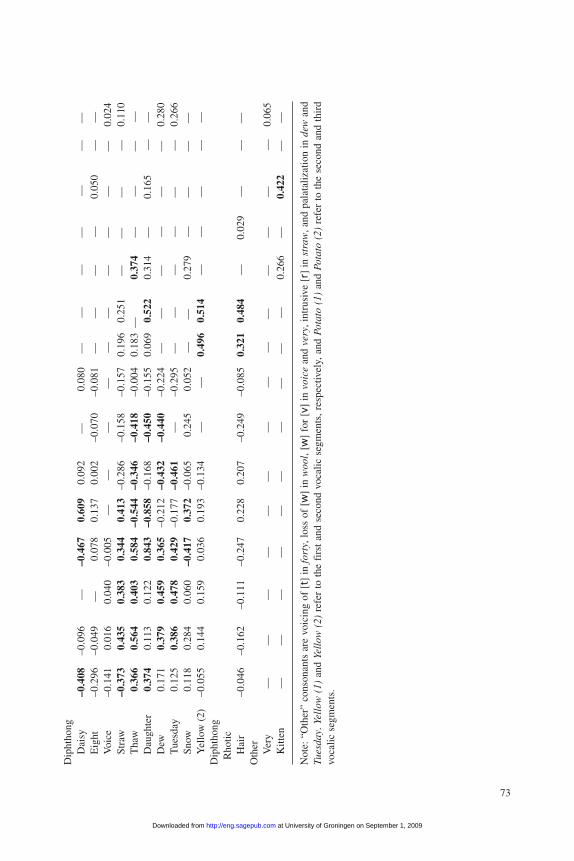
73
Dip
htho
ngD
aisy
–0.4
08–0
.096
—–0
.467
0.60
90.
092
—0.
080
——
——
——
—E
ight
–0.2
96–0
.049
—0.
078
0.13
70.
002
–0.0
70–0
.081
——
——
0.05
0—
—V
oice
–0.1
410.
016
0.04
0–0
.005
——
——
——
——
——
0.02
4St
raw
–0.3
730.
435
0.38
30.
344
0.41
3–0
.286
–0.1
58–0
.157
0.19
60.
251
——
——
0.11
0T
haw
0.36
60.
564
0.40
30.
584
–0.5
44–0
.346
–0.4
18–0
.004
0.18
3—
0.37
4—
——
—D
augh
ter
0.37
40.
113
0.12
20.
843
–0.8
58–0
.168
–0.4
50–0
.155
0.06
90.
522
0.31
4—
0.16
5—
—D
ew0.
171
0.37
90.
459
0.36
5–0
.212
–0.4
32–0
.440
–0.2
24—
——
——
—0.
280
Tue
sday
0.12
50.
386
0.47
80.
429
–0.1
77–0
.461
—–0
.295
——
——
——
0.26
6Sn
ow0.
118
0.28
40.
060
–0.4
170.
372
–0.0
650.
245
0.05
2—
—0.
279
——
——
Yel
low
(2)
–0.0
550.
144
0.15
90.
036
0.19
3–0
.134
——
0.49
60.
514
——
——
—D
ipht
hong
R
hotic
Hai
r–0
.046
–0.1
62–0
.111
–0.2
470.
228
0.20
7–0
.249
–0.0
850.
321
0.48
4—
0.02
9—
——
Oth
er Ver
y—
——
——
——
——
——
——
—0.
065
Kitt
en—
——
——
——
——
—0.
266
—0.
422
——
Not
e:“O
ther
”co
nson
ants
are
voi
cing
of
[t]
in f
orty
,los
s of
[w
] in
woo
l,[w
] fo
r [v
] in
voi
cean
d ve
ry,i
ntru
sive
[r]
in
stra
w,a
nd p
alat
aliz
atio
n in
dew
and
Tues
day.
Yel
low
(1)
and
Yell
ow (
2)re
fer
to t
he f
irst
and
sec
ond
voca
lic s
egm
ents
,res
pect
ivel
y,an
d Po
tato
(1)
and
Pota
to (
2) r
efer
to
the
seco
nd a
nd t
hird
voca
lic s
egm
ents
.
at University of Groningen on September 1, 2009 http://eng.sagepub.comDownloaded from
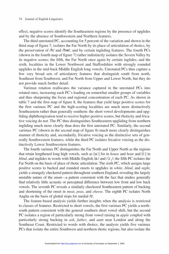
74 Journal of English Linguistics
effect, negative scores identify the Southeastern regions by the presence of upglidesand by the absence of Southwestern and Northern features.
The third unrotated PC, accounting for 5 percent of the variation and shown in thethird map of figure 7, isolates the Far North by its place of articulation of rhotics, bythe preservation of /h/ and /hw/, and by certain ingliding features. The fourth PCs(shown in the fourth map of figure 7) rather indistinctly isolates the Severn Valley byits negative scores; the fifth, the Far North once again by certain inglides; and thesixth, localities in the Lower Northwest and Staffordshire with strongly roundedupglides in the mid-back Middle English long vowels. Unrotated PCs thus capture afew very broad sets of articulatory features that distinguish south from north,Southeast from Southwest, and Far North from Upper and Lower North, but they donot provide much further detail.
Varimax rotation reallocates the variance captured in the unrotated PCs intorotated ones, increasing each PC’s loading on somewhat smaller groups of variablesand thus sharpening the focus and regional concentration of each PC. As shown intable 7 and the first map of figure 8, the features that yield large positive scores forthe first varimax PC and the high-scoring localities are much more distinctivelySoutheastern rather than generally southern: the short vowel developments and upg-liding diphthongization tend to receive higher positive scores, but rhoticity and frica-tive voicing do not. The PC thus distinguishes Southeastern upgliding from northerningliding much more clearly than does the first unrotated PC. Similarly, the secondvarimax PC (shown in the second map of figure 8) much more clearly distinguishesmanner of rhoticity and, secondarily, fricative voicing as the distinctive sets of gen-erally Southwestern features, while the third PC isolates fricative voicing as the dis-tinctively Lower Southwestern features.
The fourth varimax PC distinguishes the Far North and Upper North as the regionsthat retain lengthened long high vowels, such as [u:] for in house and hour and [i:] inblind, and inglides in words with Middle English /a:/ and /O:1/; the fifth PC isolates theFar North on the basis of place of rhotic articulation. The sixth PC, which assigns largepositive scores to backed and rounded onsets to upglides in white, blind, and night,yields a strangely checkered pattern throughout southern England, revealing the largelyunstable nature of the onset—a pattern consistent with the fact that studies generallyfind relatively little acoustic or perceptual difference between low front and low backvowels. The seventh PC reveals a similarly checkered Southeastern pattern of backingand shortening of the onset in meat, peas, and cheese. The eighth PC isolates NorthAnglia on the basis of glottal stops for medial /t/.
The feature-based analysis yields further insights when the analysis is restrictedto classes of features. Restricted to short vowels, the first varimax PC yields a north-south pattern consistent with the general southern short vowel shift, but the secondPC isolates a region of particularly strong front vowel raising in apple coupled withparticularly strong backing in ask, father, and aunt near London and along theSoutheast Coast. Restricted to words with rhotics, the analysis yields five varimaxPCs that isolate the entire Southwest and northern rhotic regions, but also isolate the
at University of Groningen on September 1, 2009 http://eng.sagepub.comDownloaded from
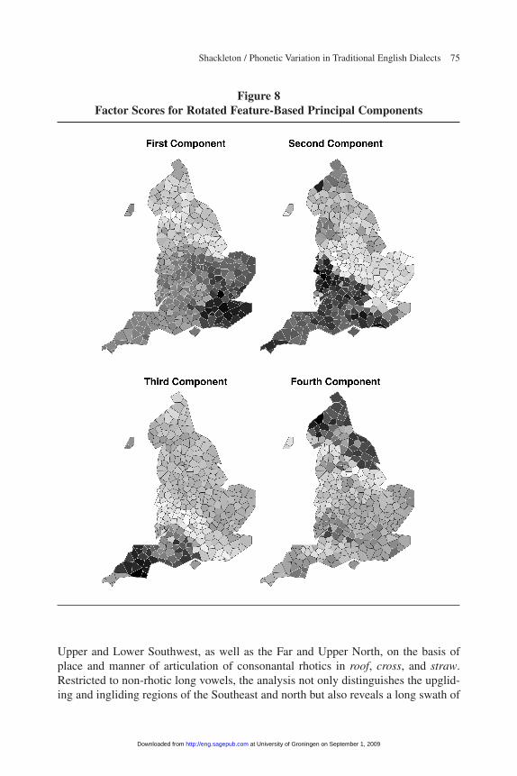
Shackleton / Phonetic Variation in Traditional English Dialects 75
Upper and Lower Southwest, as well as the Far and Upper North, on the basis ofplace and manner of articulation of consonantal rhotics in roof, cross, and straw.Restricted to non-rhotic long vowels, the analysis not only distinguishes the upglid-ing and ingliding regions of the Southeast and north but also reveals a long swath of
Figure 8Factor Scores for Rotated Feature-Based Principal Components
at University of Groningen on September 1, 2009 http://eng.sagepub.comDownloaded from
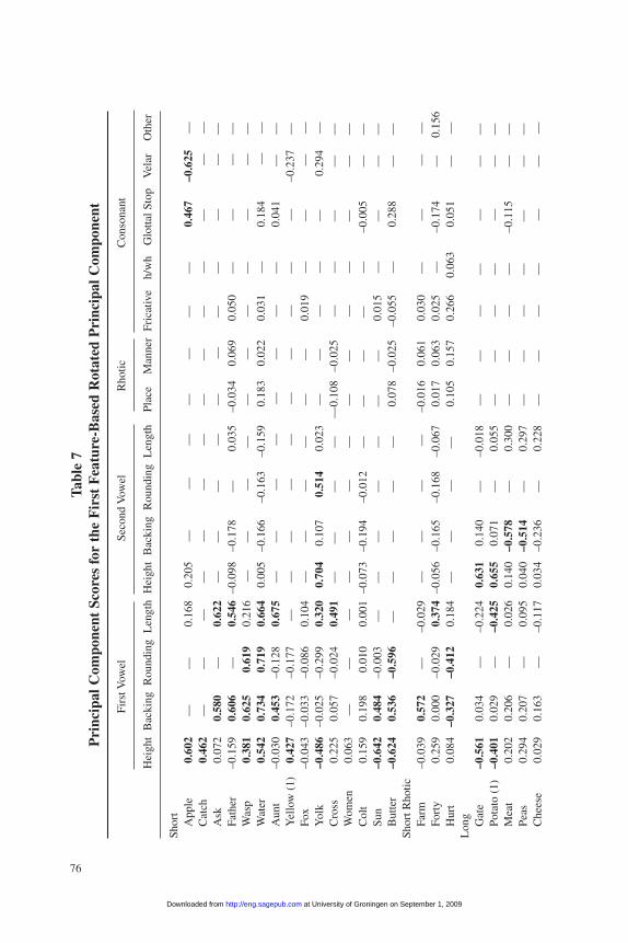
76
Tabl
e 7
Pri
ncip
al C
ompo
nent
Sco
res
for
the
Fir
st F
eatu
re-B
ased
Rot
ated
Pri
ncip
al C
ompo
nent
Firs
t Vow
elSe
cond
Vow
elR
hotic
Con
sona
nt
Hei
ght
Bac
king
Rou
ndin
gL
engt
hH
eigh
tB
acki
ngR
ound
ing
Len
gth
Plac
eM
anne
rFr
icat
ive
h/w
hG
lotta
l Sto
pV
elar
Oth
er
Shor
tA
pple
0.60
2—
—0.
168
0.20
5—
——
——
——
0.46
7–0
.625
—C
atch
0.46
2—
——
——
——
——
——
——
—A
sk0.
072
0.58
0—
0.62
2—
——
——
——
——
——
Fath
er–0
.159
0.60
6—
0.54
6–0
.098
–0.1
78—
0.03
5–0
.034
0.06
90.
050
——
——
Was
p0.
381
0.62
50.
619
0.21
6—
——
——
——
——
——
Wat
er0.
542
0.73
40.
719
0.66
40.
005
–0.1
66–0
.163
–0.1
590.
183
0.02
20.
031
—0.
184
——
Aun
t–0
.030
0.45
3–0
.128
0.67
5—
——
——
——
—0.
041
——
Yel
low
(1)
0.42
7–0
.172
–0.1
77—
——
——
——
——
—–0
.237
—Fo
x–0
.043
–0.0
33–0
.086
0.10
4—
——
——
—0.
019
——
——
Yol
k–0
.486
–0.0
25–0
.299
0.32
00.
704
0.10
70.
514
0.02
3—
——
——
0.29
4—
Cro
ss0.
225
0.05
7–0
.024
0.49
1—
——
——
0.10
8–0
.025
——
——
—W
omen
0.06
3—
——
——
——
——
——
——
—C
olt
0.15
90.
198
0.01
00.
001
–0.0
73–0
.194
–0.0
12—
——
——
–0.0
05—
—Su
n–0
.642
0.48
4–0
.003
——
——
——
—0.
015
——
——
But
ter
–0.6
240.
536
–0.5
96—
——
——
0.07
8–0
.025
–0.0
55—
0.28
8—
—Sh
ort R
hotic
Farm
–0.0
390.
572
—–0
.029
——
——
–0.0
160.
061
0.03
0—
——
—Fo
rty
0.25
90.
000
–0.0
290.
374
–0.0
56–0
.165
–0.1
68–0
.067
0.01
70.
063
0.02
5—
–0.1
74—
0.15
6H
urt
0.08
4–0
.327
–0.4
120.
184
——
——
0.10
50.
157
0.26
60.
063
0.05
1—
—L
ong
Gat
e–0
.561
0.03
4—
–0.2
240.
631
0.14
0—
–0.0
18—
——
——
——
Pota
to (
1)–0
.401
0.02
9—
–0.4
250.
655
0.07
1—
0.05
5—
——
——
——
Mea
t0.
202
0.20
6—
0.02
60.
140
–0.5
78—
0.30
0—
——
—–0
.115
——
Peas
0.29
40.
207
—0.
095
0.04
0–0
.514
—0.
297
——
——
——
—C
hees
e0.
029
0.16
3—
–0.1
170.
034
–0.2
36—
0.22
8—
——
——
——
at University of Groningen on September 1, 2009 http://eng.sagepub.comDownloaded from
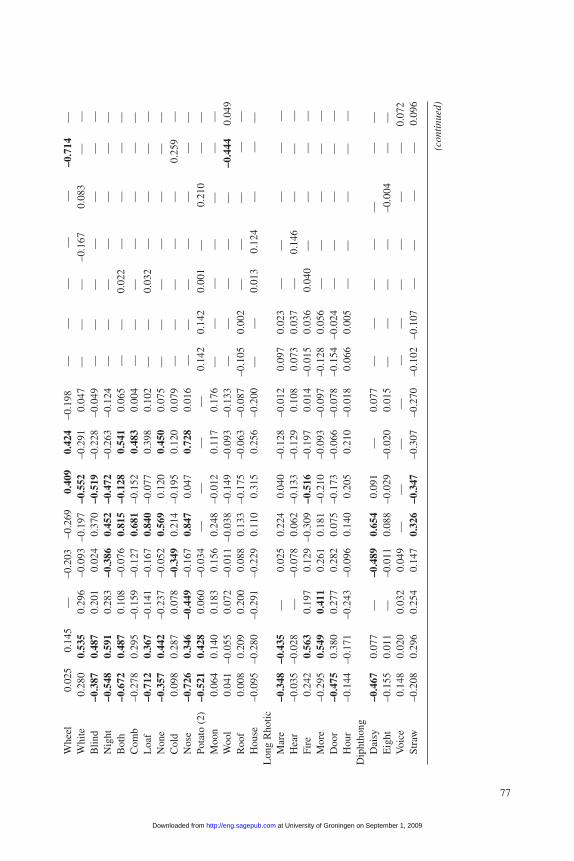
77
Whe
el0.
025
0.14
5—
–0.2
03–0
.269
0.40
90.
424
–0.1
98—
——
——
–0.7
14—
Whi
te0.
280
0.53
50.
296
–0.0
93–0
.197
–0.5
52–0
.291
0.04
7—
——
–0.1
670.
083
——
Blin
d–0
.387
0.48
70.
201
0.02
40.
370
–0.5
19–0
.228
–0.0
49—
——
——
——
Nig
ht–0
.548
0.59
10.
283
–0.3
860.
452
–0.4
72–0
.263
–0.1
24—
——
——
——
Bot
h–0
.672
0.48
70.
108
–0.0
760.
815
–0.1
280.
541
0.06
5—
—0.
022
——
——
Com
b–0
.278
0.29
5–0
.159
–0.1
270.
681
–0.1
520.
483
0.00
4—
——
——
——
Loa
f–0
.712
0.36
7–0
.141
–0.1
670.
840
–0.0
770.
398
0.10
2—
—0.
032
——
——
Non
e–0
.357
0.44
2–0
.237
–0.0
520.
569
0.12
00.
450
0.07
5—
——
——
——
Col
d0.
098
0.28
70.
078
–0.3
490.
214
–0.1
950.
120
0.07
9—
——
——
0.25
9—
Nos
e–0
.726
0.34
6–0
.449
–0.1
670.
847
0.04
70.
728
0.01
6—
——
——
——
Pota
to (
2)–0
.521
0.42
80.
060
–0.0
34—
——
—0.
142
0.14
20.
001
—0.
210
——
Moo
n0.
064
0.14
00.
183
0.15
60.
248
–0.0
120.
117
0.17
6—
——
——
——
Woo
l0.
041
–0.0
550.
072
–0.0
11–0
.038
–0.1
49–0
.093
–0.1
33—
——
——
–0.4
440.
049
Roo
f0.
008
0.20
90.
200
0.08
80.
133
–0.1
75–0
.063
–0.0
87–0
.105
0.00
2—
——
——
Hou
se–0
.095
–0.2
80–0
.291
–0.2
290.
110
0.31
50.
256
–0.2
00—
—0.
013
0.12
4—
——
Lon
g R
hotic
Mar
e–0
.348
–0.4
35—
0.02
50.
224
0.04
0–0
.128
–0.0
120.
097
0.02
3—
——
——
Hea
r–0
.035
–0.0
28—
–0.0
780.
062
–0.1
33–0
.129
0.10
80.
073
0.03
7—
0.14
6—
——
Fire
0.24
20.
563
0.19
70.
129
–0.3
09–0
.516
–0.1
970.
014
–0.0
150.
036
0.04
0—
——
—M
ore
–0.2
950.
549
0.41
10.
261
0.18
1–0
.210
–0.0
93–0
.097
–0.1
280.
056
——
——
—D
oor
–0.4
750.
380
0.27
70.
282
0.07
5–0
.173
–0.0
66–0
.078
–0.1
54–0
.024
——
——
—H
our
–0.1
44–0
.171
–0.2
43–0
.096
0.14
00.
205
0.21
0–0
.018
0.06
60.
005
——
——
—D
ipht
hong
Dai
sy–0
.467
0.07
7—
–0.4
890.
654
0.09
1—
0.07
7—
——
——
——
Eig
ht–0
.155
0.01
1—
–0.0
110.
088
–0.0
29–0
.020
0.01
5—
——
—–0
.004
——
Voi
ce0.
148
0.02
00.
032
0.04
9—
——
——
——
——
—0.
072
Stra
w–0
.208
0.29
60.
254
0.14
70.
326
–0.3
47–0
.307
–0.2
70–0
.102
–0.1
07—
——
—0.
096
(con
tinu
ed)
at University of Groningen on September 1, 2009 http://eng.sagepub.comDownloaded from

78
Tabl
e 7
(con
tinu
ed)
Firs
t Vow
elSe
cond
Vow
elR
hotic
Con
sona
nt
Hei
ght
Bac
king
Rou
ndin
gL
engt
hH
eigh
tB
acki
ngR
ound
ing
Len
gth
Plac
eM
anne
rFr
icat
ive
h/w
hG
lotta
l Sto
pV
elar
Oth
er
Tha
w0.
162
0.36
50.
241
0.32
5–0
.245
–0.2
03–0
.210
–0.0
210.
424
—0.
398
——
——
Dau
ghte
r0.
398
0.20
90.
198
0.66
9–0
.682
–0.0
67–0
.316
–0.1
430.
016
0.03
30.
006
—0.
195
——
Dew
0.09
50.
144
0.13
90.
030
–0.0
53–0
.147
–0.1
240.
039
——
——
——
–0.0
75T
uesd
ay0.
090
0.16
60.
191
0.09
6–0
.063
–0.2
01—
–0.0
15—
——
——
—–0
.051
Snow
–0.1
870.
168
–0.1
48–0
.578
0.63
3–0
.100
0.41
0–0
.032
——
0.02
3—
——
—Y
ello
w (
2)–0
.198
0.14
30.
188
0.03
80.
323
–0.1
02—
—0.
106
0.11
5—
——
——
Dip
htho
ng
Rho
ticH
air
–0.1
51–0
.222
–0.0
54–0
.150
0.15
9–0
.032
–0.1
940.
072
0.22
5–0
.011
—0.
181
——
—O
ther Ver
y—
——
——
——
——
——
——
—0.
089
Kitt
en—
——
——
——
——
—0.
046
—0.
355
——
Not
e:“O
ther
”co
nson
ants
are
voi
cing
of
[t]
in fo
rty,
loss
of
[w]
in w
ool,
[w]
for
[v]
in v
oice
and
very
,int
rusi
ve [r]
in s
traw
,and
pal
atal
izat
ion
in d
ewan
dTu
esda
y. Y
ello
w (
1)an
d Ye
llow
(2)
refe
r to
the
firs
t and
sec
ond
voca
lic s
egm
ents
,res
pect
ivel
y,an
d Po
tato
(1)
and
Pota
to (
2) r
efer
to th
e se
cond
and
thir
dvo
calic
seg
men
ts.
at University of Groningen on September 1, 2009 http://eng.sagepub.comDownloaded from
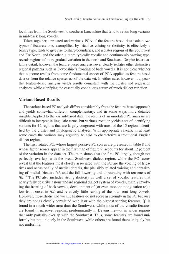
Shackleton / Phonetic Variation in Traditional English Dialects 79
localities from the Southwest to southern Lancashire that tend to retain long variantsin mid-back long vowels.
Taken together, unrotated and varimax PCA of the feature-based data isolate twotypes of features: one, exemplified by fricative voicing or rhoticity, is effectively abinary type, tends to give rise to sharp boundaries, and isolates regions of the Southwestand Far North; and the other, a more typically vocalic and continuously varying type,reveals regions of more gradual variation in the north and Southeast. Despite its articu-latory detail, however, the feature-based analysis never clearly isolates other distinctiveregional patterns such as Devonshire’s fronting of back vowels. It is not clear whetherthat outcome results from some fundamental aspect of PCA applied to feature-baseddata or from the relative sparseness of the data set. In either case, however, it appearsthat feature-based analysis yields results consistent with the cluster and regressionanalyses, while clarifying the essentially continuous nature of much dialect variation.
Variant-Based Results
The variant-based PC analysis differs considerably from the feature-based approachand yields somewhat different, complementary, and in some ways more detailedinsights. Applied to the variant-based data, the results of an unrotated PC analysis aredifficult to interpret in linguistic terms, but varimax rotation yields a set of identifyingvariants for 12 regions that are largely congruent with most of the 15 regions identi-fied by the cluster and phylogenetic analyses. With appropriate caveats, in at leastsome cases the variants may arguably be said to characterize a traditional Englishdialect region.
The first rotated PC, whose largest positive PC scores are presented in table 8 andwhose factor scores appear in the first map of figure 9, accounts for about 12 percentof the variation in the data set. The map shows that the first PC largely, though notperfectly, overlaps with the broad Southwest dialect region, while the PC scoresreveal that the features most closely associated with the PC are the voicing of frica-tives and occasionally of medial dentals, the plausibly related voicing and dentaliz-ing of medial fricative /s/, and the full lowering and unrounding with tenseness of/u/.35 The PC also includes strong rhoticity as well a set of vocalic features thatnearly fully describe a nonstandard regional dialect system of vowels, mainly involv-ing the fronting of back vowels, development of (or even monophthongization to) alow-front onset in /i:/, and relatively little raising of the low-front long vowels.However, those rhotic and vocalic features do not score as strongly in the PC becausethey are not as closely correlated with it or with the highest scoring features: [r] isfound in a much wider area than the Southwest, while most of the vocalic featuresare found in narrower regions, predominantly in Devonshire—or in wider regionsthat only partially overlap with the Southwest. Thus, some features are found uni-formly but not uniquely in the Southwest, while others are found there uniquely butnot uniformly.
at University of Groningen on September 1, 2009 http://eng.sagepub.comDownloaded from
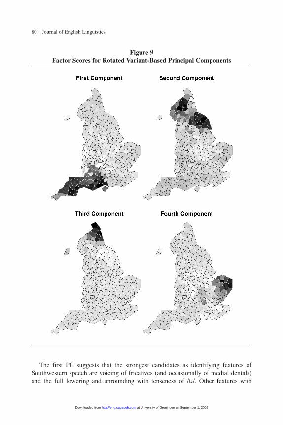
80 Journal of English Linguistics
The first PC suggests that the strongest candidates as identifying features ofSouthwestern speech are voicing of fricatives (and occasionally of medial dentals)and the full lowering and unrounding with tenseness of /u/. Other features with
Figure 9Factor Scores for Rotated Variant-Based Principal Components
at University of Groningen on September 1, 2009 http://eng.sagepub.comDownloaded from
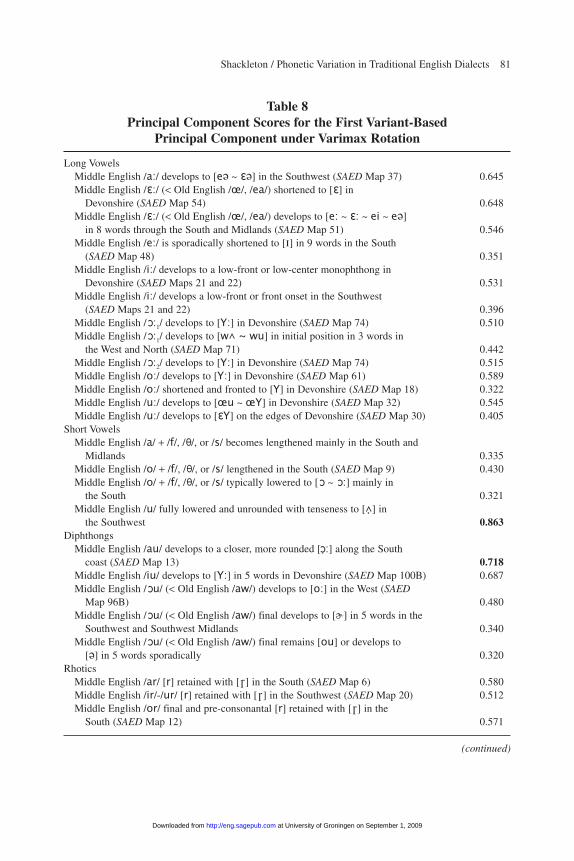
Shackleton / Phonetic Variation in Traditional English Dialects 81
Table 8Principal Component Scores for the First Variant-Based
Principal Component under Varimax Rotation
Long VowelsMiddle English /a:/ develops to [e« ~ E«] in the Southwest (SAED Map 37) 0.645Middle English /E:/ (< Old English /œ/, /ea/) shortened to [E] in
Devonshire (SAED Map 54) 0.648Middle English /E:/ (< Old English /œ/, /ea/) develops to [e: ~ E: ~ ei ~ e«]
in 8 words through the South and Midlands (SAED Map 51) 0.546Middle English /e:/ is sporadically shortened to [I] in 9 words in the South
(SAED Map 48) 0.351Middle English /i:/ develops to a low-front or low-center monophthong in
Devonshire (SAED Maps 21 and 22) 0.531Middle English /i:/ develops a low-front or front onset in the Southwest
(SAED Maps 21 and 22) 0.396Middle English /O:1/ develops to [Y:] in Devonshire (SAED Map 74) 0.510Middle English /O:1/ develops to [w^ ~ wu] in initial position in 3 words in
the West and North (SAED Map 71) 0.442Middle English /O:2/ develops to [Y:] in Devonshire (SAED Map 74) 0.515Middle English /o:/ develops to [Y:] in Devonshire (SAED Map 61) 0.589Middle English /o:/ shortened and fronted to [Y] in Devonshire (SAED Map 18) 0.322Middle English /u:/ develops to [œu ~ œY] in Devonshire (SAED Map 32) 0.545Middle English /u:/ develops to [EY] on the edges of Devonshire (SAED Map 30) 0.405
Short VowelsMiddle English /a/ + /f/, /Q/, or /s/ becomes lengthened mainly in the South and
Midlands 0.335Middle English /o/ + /f/, /Q/, or /s/ lengthened in the South (SAED Map 9) 0.430Middle English /o/ + /f/, /Q/, or /s/ typically lowered to [O ~ O:] mainly in
the South 0.321Middle English /u/ fully lowered and unrounded with tenseness to [ .̂ ] in
the Southwest 0.863Diphthongs
Middle English /au/ develops to a closer, more rounded [ cO:] along the South coast (SAED Map 13) 0.718
Middle English /iu/ develops to [Y:] in 5 words in Devonshire (SAED Map 100B) 0.687Middle English /Ou/ (< Old English /aw/) develops to [o:] in the West (SAED
Map 96B) 0.480Middle English /Ou/ (< Old English /aw/) final develops to [e] in 5 words in the
Southwest and Southwest Midlands 0.340Middle English /Ou/ (< Old English /aw/) final remains [ou] or develops to
[«] in 5 words sporadically 0.320Rhotics
Middle English /ar/ [r] retained with [r] in the South (SAED Map 6) 0.580Middle English /ir/-/ur/ [r] retained with [r] in the Southwest (SAED Map 20) 0.512Middle English /or/ final and pre-consonantal [r] retained with [r] in the
South (SAED Map 12) 0.571
(continued)
at University of Groningen on September 1, 2009 http://eng.sagepub.comDownloaded from

82 Journal of English Linguistics
positive scores are also diagnostic but not necessarily defining. That result is con-sistent with Trudgill’s (1999) association of [z] in seven with this dialect region.
Although it clearly identifies a number of variants associated with the region, nei-ther the PC nor its associated variants is replicated perfectly in any singleSouthwestern locality, and they can only rather loosely be thought of as representinga Southwestern dialect or even a group of dialects. Even the voicing of fricativesappears in only about three quarters of possible occurrences in the Southwesternlocalities. No locality in the Southwest, not even the most typical Southwesterner,uses all of the variants with PC scores above 0.32 in the first rotated PC, and barelyany of the localities even use a majority of them. Not much more than half of thevariants associated with the PC occur even in the locality with the highest factorscore for the first PC; conversely, roughly 20 percent of the variants occur in severalof the lowest scoring localities, which tend to be somewhat further north in the WestMidlands region. At the same time, the PC excludes a large number of variants thatare widely used throughout the Southwest: strikingly, it does not include a singlevariant that is the most common Southwestern pronunciation of a Middle Englishlong vowel. Because their distributions very rarely closely overlap with the bound-aries of the Southwest, most variants that might constitute a vowel system commonto most of the Southwest do not in fact appear as part of the Southwestern PC. Suchlimitations appear to be inherent in the use of principal components or factor analy-sis in the analysis of linguistic variation, and they underline the fact that systematicvariation is the exception rather than the rule in the traditional dialects.
The second rotated PC, whose factor scores are shown in the second map offigure 9, accounts for about 6 percent of the variation in the data set. It appears to bestrongly associated with most but not all of the Cumbria–North Yorkshire subregion
Table 8 (continued)
ConsonantsMiddle English /f/ (> Old English /f/) develops to [v] in the Southwest
(SAED Map 105) 0.970Middle English /f/ (> Old French /f/) develops to [v] in the Southwest
(SAED Map 106) 0.872Middle English /s/ (> Old English /s/) develops to [z] in the Southwest
(SAED Map 107) 0.977Middle English /s/ (> Old French /s/) develops to [z] in the Southwest
(SAED Map 108) 0.896Middle English /Q/ develops to [ð] in the Southwest (SAED Map 109) 0.973Middle English /Qr/ develops to [dr ~ ðr] in the Southwest (SAED Map 110) 0.962ME medial /t/ develops to [d] along the southern coast 0.841ME medial /s/ develops to [d] in isn’t, wasn’t, doesn’t, and hasn’t
(4 instances) in the Southwest 0.721Middle English /h/ retained in the Southwest (SAED Map 111) 0.477Middle English /w/ lost before /u/ in the Southwest (SAED Map 114) 0.417
at University of Groningen on September 1, 2009 http://eng.sagepub.comDownloaded from
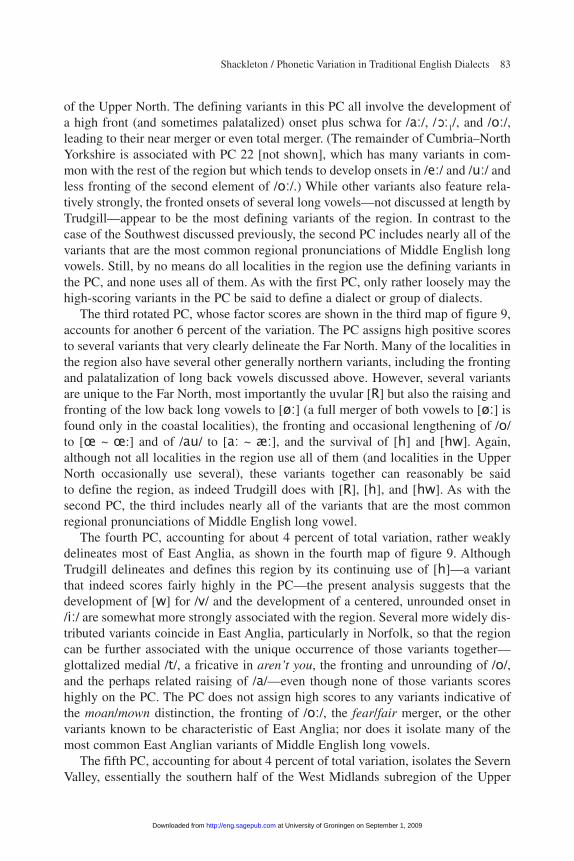
Shackleton / Phonetic Variation in Traditional English Dialects 83
of the Upper North. The defining variants in this PC all involve the development ofa high front (and sometimes palatalized) onset plus schwa for /a:/, /O:1/, and /o:/,leading to their near merger or even total merger. (The remainder of Cumbria–NorthYorkshire is associated with PC 22 [not shown], which has many variants in com-mon with the rest of the region but which tends to develop onsets in /e:/ and /u:/ andless fronting of the second element of /o:/.) While other variants also feature rela-tively strongly, the fronted onsets of several long vowels—not discussed at length byTrudgill—appear to be the most defining variants of the region. In contrast to thecase of the Southwest discussed previously, the second PC includes nearly all of thevariants that are the most common regional pronunciations of Middle English longvowels. Still, by no means do all localities in the region use the defining variants inthe PC, and none uses all of them. As with the first PC, only rather loosely may thehigh-scoring variants in the PC be said to define a dialect or group of dialects.
The third rotated PC, whose factor scores are shown in the third map of figure 9,accounts for another 6 percent of the variation. The PC assigns high positive scoresto several variants that very clearly delineate the Far North. Many of the localities inthe region also have several other generally northern variants, including the frontingand palatalization of long back vowels discussed above. However, several variantsare unique to the Far North, most importantly the uvular [R] but also the raising andfronting of the low back long vowels to [ø:] (a full merger of both vowels to [ø:] isfound only in the coastal localities), the fronting and occasional lengthening of /o/to [œ ~ œ:] and of /au/ to [a: ~ æ:], and the survival of [h] and [hw]. Again,although not all localities in the region use all of them (and localities in the UpperNorth occasionally use several), these variants together can reasonably be said to define the region, as indeed Trudgill does with [R], [h], and [hw]. As with the second PC, the third includes nearly all of the variants that are the most commonregional pronunciations of Middle English long vowel.
The fourth PC, accounting for about 4 percent of total variation, rather weaklydelineates most of East Anglia, as shown in the fourth map of figure 9. AlthoughTrudgill delineates and defines this region by its continuing use of [h]—a variantthat indeed scores fairly highly in the PC—the present analysis suggests that thedevelopment of [w] for /v/ and the development of a centered, unrounded onset in/i:/ are somewhat more strongly associated with the region. Several more widely dis-tributed variants coincide in East Anglia, particularly in Norfolk, so that the regioncan be further associated with the unique occurrence of those variants together—glottalized medial /t/, a fricative in aren’t you, the fronting and unrounding of /o/,and the perhaps related raising of /a/—even though none of those variants scoreshighly on the PC. The PC does not assign high scores to any variants indicative ofthe moan/mown distinction, the fronting of /o:/, the fear/fair merger, or the othervariants known to be characteristic of East Anglia; nor does it isolate many of themost common East Anglian variants of Middle English long vowels.
The fifth PC, accounting for about 4 percent of total variation, isolates the SevernValley, essentially the southern half of the West Midlands subregion of the Upper
at University of Groningen on September 1, 2009 http://eng.sagepub.comDownloaded from
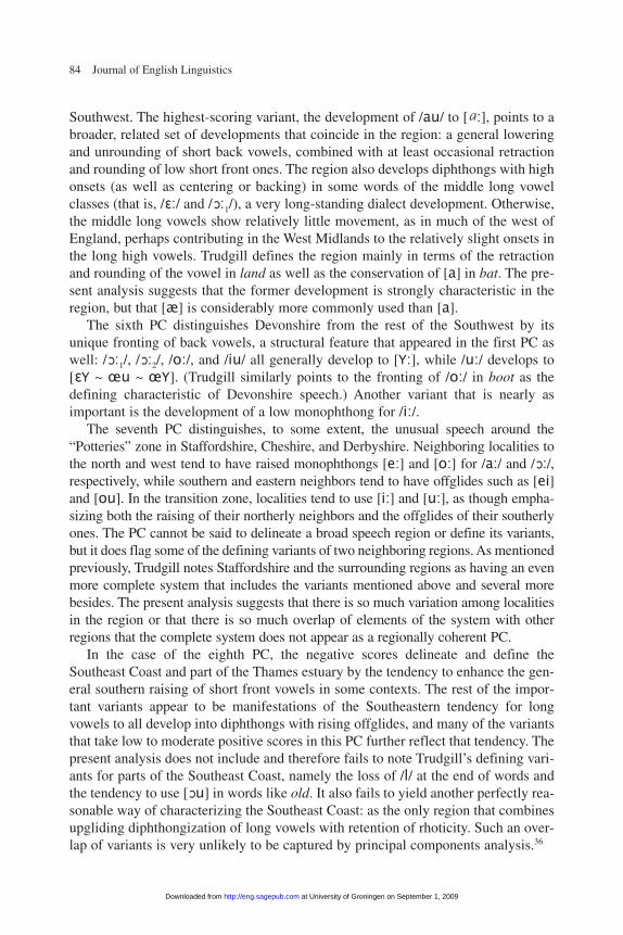
84 Journal of English Linguistics
Southwest. The highest-scoring variant, the development of /au/ to [ :], points to abroader, related set of developments that coincide in the region: a general loweringand unrounding of short back vowels, combined with at least occasional retractionand rounding of low short front ones. The region also develops diphthongs with highonsets (as well as centering or backing) in some words of the middle long vowelclasses (that is, /E:/ and /O:1/), a very long-standing dialect development. Otherwise,the middle long vowels show relatively little movement, as in much of the west ofEngland, perhaps contributing in the West Midlands to the relatively slight onsets inthe long high vowels. Trudgill defines the region mainly in terms of the retractionand rounding of the vowel in land as well as the conservation of [a] in bat. The pre-sent analysis suggests that the former development is strongly characteristic in theregion, but that [æ] is considerably more commonly used than [a].
The sixth PC distinguishes Devonshire from the rest of the Southwest by itsunique fronting of back vowels, a structural feature that appeared in the first PC aswell: /O:1/, /O:2/, /o:/, and /iu/ all generally develop to [Y:], while /u:/ develops to[EY ~ œu ~ œY]. (Trudgill similarly points to the fronting of /o:/ in boot as thedefining characteristic of Devonshire speech.) Another variant that is nearly asimportant is the development of a low monophthong for /i:/.
The seventh PC distinguishes, to some extent, the unusual speech around the“Potteries” zone in Staffordshire, Cheshire, and Derbyshire. Neighboring localities tothe north and west tend to have raised monophthongs [e:] and [o:] for /a:/ and /O:/,respectively, while southern and eastern neighbors tend to have offglides such as [ei]and [ou]. In the transition zone, localities tend to use [i:] and [u:], as though empha-sizing both the raising of their northerly neighbors and the offglides of their southerlyones. The PC cannot be said to delineate a broad speech region or define its variants,but it does flag some of the defining variants of two neighboring regions. As mentionedpreviously, Trudgill notes Staffordshire and the surrounding regions as having an evenmore complete system that includes the variants mentioned above and several morebesides. The present analysis suggests that there is so much variation among localitiesin the region or that there is so much overlap of elements of the system with otherregions that the complete system does not appear as a regionally coherent PC.
In the case of the eighth PC, the negative scores delineate and define theSoutheast Coast and part of the Thames estuary by the tendency to enhance the gen-eral southern raising of short front vowels in some contexts. The rest of the impor-tant variants appear to be manifestations of the Southeastern tendency for longvowels to all develop into diphthongs with rising offglides, and many of the variantsthat take low to moderate positive scores in this PC further reflect that tendency. Thepresent analysis does not include and therefore fails to note Trudgill’s defining vari-ants for parts of the Southeast Coast, namely the loss of /l/ at the end of words andthe tendency to use [Ou] in words like old. It also fails to yield another perfectly rea-sonable way of characterizing the Southeast Coast: as the only region that combinesupgliding diphthongization of long vowels with retention of rhoticity. Such an over-lap of variants is very unlikely to be captured by principal components analysis.36
a
at University of Groningen on September 1, 2009 http://eng.sagepub.comDownloaded from
Shackleton / Phonetic Variation in Traditional English Dialects 85
The negative scores of the ninth PC define another region of the EnglishSoutheast—in this case, the Central Southeast region around and to the north ofLondon—by a process of diphthongization. The defining characteristic appears to bea tendency to front and lower the first elements of some of the diphthongs, such as[æi ~ ai] for /a:/ and especially [«u ~ Uu ~ æu] for /O:1/. The results are consistentwith the hypothesis that the diphthongization is a long-term, ongoing process cen-tered near the metropolis, and that older forms are preserved in the periphery. (Thefact that the progressive elements are typically not found in American speech butregularly appear in English-speaking countries settled more recently may providesome confirmation for that hypothesis.) The analysis fails to capture the moan/mowndistinction noted in this region by Trudgill.
The tenth PC delineates southern Lancashire, a portion of the Lower North, by thesame variant noted by Trudgill: its localities’ use of an alveolar approximant rhotic.The eleventh PC rather poorly delineates the northern half of the West Midlands, alongwith parts of the Lower North, by the retention of a long monophthong for the low longvowels, as mentioned in the discussion of the seventh PC describing the transition zonebetween those regions and the Midlands proper. The twelfth PC, characterized not onlyby the use of the retroflex [r] but also by the tendency to insert it in such words as win-dow, does not really delineate any dialect region, but it tends to take moderately highvalues through a broad swath of the Upper Southwest and the Southeast Coast, tracingthe southern edge of the major boundary of rhoticity in the South of England, theWessex Line. The PC highlights the region of competition between rhotic and non-rhotic variants, where rhotic speakers tend to overcompensate by inserting rhoticswhere they are otherwise absent.
The thirteenth PC clearly delineates Lincolnshire as the region which combines atendency to develop a low-center onset to the high long vowels with a tendency todevelop centering diphthongs for the low and middle long vowels (and withoutstrongly raising them). The fourteenth PC isolates and defines south Yorkshire by itsunique front upglides in the long low back vowels, and the fifteenth does the samefor north Lancashire and environs (the Upper Northeast) by its tendency to merge/O:1/ and /a:/ into a falling diphthong [ia ~ ea]. Beyond those, the PCs becomeincreasingly uninformative: the sixteenth isolates a dozen localities in the SoutheastCoast region that use a rhotic approximant; the seventeenth isolates Cumberland 1by its unique use of a rhotic trill; and the eighteenth isolates some western localitiesthat use a retracted, rounded vowel in hand.
In sum, PCA identifies sets of identifying variants for more than a dozen regionslargely congruent with many of the 15 regions identified by the cluster and phylogeneticanalyses, in the process accounting for roughly half the variation in the data set. In at least some cases, the PCs appear to provide a fairly objective method for character-izing the traditional English dialect regions on a quantitative basis, providing signifi-cantly more detailed insight than the feature-based PCA. However, the PCs often isolatevariants that are unique to a fairly small subregion, and they often include variants thatare widely used throughout the relevant region but that are not unique to it. No locality
at University of Groningen on September 1, 2009 http://eng.sagepub.comDownloaded from
86 Journal of English Linguistics
in a region uses all of the variants identified by the relevant PC, and few even use mostof them. With the exception of three PCs that are composed of variants found inDevonshire, Lincolnshire, and the Far North, respectively, none of the PCs isolatesextensive sets of variants that could be considered even partial systems of vowels uniqueto particular regions of England.
Variant-Based Principal Components and Variant Frequency
Additional context for the results of the PC analysis can be derived by examiningthe frequency of the two most common modern regional variants in each region ofmost of the Middle English phonemes examined in this study. Regions do indeed tendto have fairly uniform speech patterns: the two most frequent variants in each categoryaccount for at least 91 percent and as much as 98 percent of all usage in their respec-tive regions. The most extensive intraregional variation occurs among descendants ofMiddle English long vowels and, to a lesser extent, diphthongs. The regions identifiedby distance measures, distance regressions, and variant-area regressions as having thegreatest variation—the Lower Northwest, the West Midlands, and the Central South—are the regions that have a large number of relatively low-frequency variants for theMiddle English long vowels. With a few exceptions, variant usage for short vowels andconsonants tends to be relatively uniform in each region. Although variant usage is rel-atively uniform within a given region, however, very few common variants are uniqueto a specific region: in the great majority of cases, variants are found in two or moreregions. There is therefore relatively little scope for PC analysis to identify regionsthrough variants that are unique to them. Nevertheless, even though any given varianttends to be found in a number of regions, each region has a relatively unique overallpattern of frequently used variants.
These frequency details help explain the efficacy and limitations of the PC analy-sis in identifying unique or important regional variants. The PCs discussed in theprevious section identify many of the regionally most common variants and nearlyone third of the regionally most common long vowels and diphthongs. In 3 of the 15regions—Cumbria–North Yorkshire, Lincolnshire, and Devonshire, linguisticallyamong the most uniform regions—PCs isolate 8 of the 12 most common long vowelsand diphthongs. However, in 3 other regions in the transitional center of the country—Staffordshire, the East Midlands, and the Central South—PCs fail to isolate a singleone (though one PC identifies a number of less common variants in northernStaffordshire). Moreover, about one third of the variants isolated by the PC analysisare forms that are fairly uncommon even in the region or regions in which theyappear. Equally importantly, only about one quarter of the variants that appear in aPC and that are among the two regionally most common variants for a MiddleEnglish phoneme can be more or less uniquely associated with a specific region: theremaining three quarters are common in more than one region, and in a number ofcases they are identified by more than one PC in more than one region. For example,
at University of Groningen on September 1, 2009 http://eng.sagepub.comDownloaded from
Shackleton / Phonetic Variation in Traditional English Dialects 87
the development of a low-front or front onset (i.e., [ai ~ Ei]) for Middle English /i:/appears in the second PC as a characteristic of some importance in the Far North,where it is ubiquitous. However, it also features in the third PC as a feature of mar-ginal importance in Cumbria–North Yorkshire, where it is also practically ubiqui-tous, and it surfaces yet again in the thirteenth PC as a feature of Lincolnshirespeech, where it appears with a frequency of 69 percent.
In short, PCs rarely isolate linguistic structures, variants, or features that areunique to regions. Nevertheless, they do tend to isolate sets of variants or featuresthat are associated with regions, and a robust general characterization of regionalvarieties of English usage emerges from the insights from the PC analysis and anexamination of the regional distribution of variants.
Conclusions
In summary, the quantitative tools presented here yield reasonable measures ofvariation in phonetic usage among English localities, illustrate the largely continu-ous geographical nature of that variation (particularly with respect to vocalic fea-tures), identify a score of major and minor dialect regions as clusters of localitieswith relatively similar patterns of usage, distinguish regions of relative uniformityfrom transitional zones with substantially greater variation, and isolate regionallycoherent groups of features that can be said, with appropriate caveats, to distinguishseveral but by no means all of the dialect regions. The results largely corroboratestandard characterizations in the literature but differ from those previous studies inseveral cases in the placement of several important dialect boundaries, in the associ-ation of features with dialects, and in placing those systematic characteristics againsta background of largely continuous variation. The techniques reinforce each other toprovide a consistent picture of the traditional English usages, tending to confirm theapplicability of computational techniques to the study of dialect variation.
All of the techniques appear useful, though they need not all be used in concert.The results suggest that even a small but judiciously chosen feature-based data setcan yield a great deal of insight, and that in the absence of feature detail, variant-based data also can be used quite effectively. Clustering techniques are useful fordelineating dialect regions, but they do not necessarily distinguish between regionsof greater uniformity and greater diversity—a task for which distance regressions,variant-area regressions, and barrier analysis are more suitable, and any one of whichis likely to be sufficient. Finally, principal components analysis appears to be usefulin isolating distinctive features or variants that are more or less characteristic ofdialect regions. The technique may be equally applicable to the study of linguisticvariation across class, gender, and other dimensions as well. In some circumstances,feature-based PCA may not only capture structural features such as upgliding or ing-liding, but also provide measures of their strength, while variant-based PCA may
at University of Groningen on September 1, 2009 http://eng.sagepub.comDownloaded from
88 Journal of English Linguistics
isolate groups of variants that reflect structural shifts. In this respect, feature-basedand variant-based approaches may be complements rather than substitutes.
Taken together, the results provide a phonetic basis for the following tentativeclassification of the traditional English dialects and dialect regions.
The relatively uniform Far North is distinguished from the rest of the countrymost notably by its use of uvular [R], the Northumbrian burr. However, the regionalso features the survival of [h] and [hw]—features that are occasional but increas-ingly uncommon as one moves further south—as well as the fairly common merger,raising, and fronting of the low back long vowels to [ø:], and the fronting and occa-sional lengthening of /o/ to [œ ~ œ:] and of /au/ to [a: ~ æ:]. As in most of thenorth of England, the Middle English qualities of short vowels tend to be conserved.
The Upper North develops centering diphthongs for most of the long vowels.Cumbria–North Yorkshire is characterized by the development of a high front (andsometimes palatalized) onset plus inglide for /a:/, /O:1/, and /o:/, leading to a signif-icant degree of merger. The Upper Northwest shows a similar development for /a:/and /O:1/, except that the glides are to a lower, more fronted [a] rather than [«]. Bothregions show the occasional development of /o:/ to [jV ~ iø].
The Lower North combines a tendency to develop the high long vowels intoupglides with a low-center onset with a tendency to develop centering diphthongs forthe low and middle long vowels without strongly raising them. The Lower Northwestis also characterized, in the west, by use of an alveolar approximant rhotic, and inthe east by fronted upglides in the long low back vowels. Lincolnshire has practicallyno unique features, save perhaps the merging of /a:/ and /ai/ to [e« ~ E«], yet has asufficiently unique and uniform combination of variants that it can be clearly iden-tified by a variant-based PC.
The Central Midlands witness such widely used and incoherently distributedvariants and features that PC analysis cannot uncover definitive sets, but the regioncan generally be identified by the unique overlapping of northern retention of olderforms for the short vowels and the southeastern innovations in the long vowels dis-cussed below.38 The East Midlands—in many ways, the heart of the English dialectworld, with many of the most typical localities in the SED and a highly uniform pat-tern of speech—never scores highly in any principal component. Staffordshireappears as an island of relative uniformity in an important transition zone withunusual variability, but several techniques suggest that a “Potteries” system is notevident in the SED data, though principal components analysis isolates a componentof it in the northern part of the region.
The Upper Southwest sees the most northerly expressions of several southerncharacteristics, including rhoticity and short vowel shifts. The West Midlands arecharacterized by a general lowering and unrounding of short back vowels, occa-sional retraction and rounding of low short front ones, occasional high onsets inwords with the middle long vowels, and little movement otherwise. The CentralSouth proves to be a highly variable, transitional region whose variants are in somecases too widespread and in other cases too infrequent to identify it. An examination
at University of Groningen on September 1, 2009 http://eng.sagepub.comDownloaded from
Shackleton / Phonetic Variation in Traditional English Dialects 89
of common features suggests that the Central South combines southern shifts inshort vowels and retention of rhoticity with minor northern tendencies to developinglides in long vowels.
The Southeast sees extensive shifts in the Middle English short vowels as well asthe development of the Middle English long vowels into coherent systems of upg-liding diphthongs that are strongly evident in several of the variant-based and feature-based principal components. North Anglia appears best defined by a hodge-podge of unique features, including the glottalization of medial /t/; the developmentof [w] for /v/; the development of a centered, unrounded onset in /i:/; and the con-tinuing use of [h], but the analysis fails to identify several other distinctively EastAnglian features. The Central Southeast is distinguished by the tendency to exag-gerate the fronting and lowering of the first elements of some of the upgliding diph-thongs, such as [æi ~ ai] for /a:/ and especially [«u ~ Uu ~ æu] for /O:1/, while theSoutheast Coast is distinguished by the tendency to enhance the general southernraising of short front vowels in at least some contexts combined with retention ofrhoticity. L-vocalization appears with relatively high frequency in the latter tworegions as well.
The Lower Southwest appears best defined by the voicing of fricatives and occa-sionally of medial dentals, the voicing and dentalizing of medial fricative [s], andthe full lowering and unrounding of /u/. Along with much of the Upper Southwestand the Southeast Coast, the Lower Southwest retains a fully retroflex rhoticity aftervowels. The Central Southwest has little that is unique about it, tending to have fea-tures that overlap with those in neighboring regions, while Cornwall has little to dis-tinguish it from the Central Southwest except its lower frequency of fricativevoicing. Devonshire is distinguished from the rest of the Southwest by its uniquefronting of back vowels and the development of a low monophthong for /i:/.
The neatness of these tentative classifications should not obscure the largely con-tinuous and often unsystematic nature of phonetic variation across England. Even inregions with relatively uniform speech, few localities—not even those localities thatcan be characterized as having speech most typical of their regions—adhere rigidly tothe patterns uncovered by any quantitative approach. Regional speech patterns appearto be only rather loosely characterized by the patterns in their associated principalcomponents, by the speech patterns of their most typical localities, or by average fre-quencies of occurrence of features. In linguistics as in biology, variation abounds, andtype specimens are necessarily arbitrarily chosen.
Appendix A: Variables Used in the Feature-Based Approach
Table A-1 shows the features in 55 words that are used to analyze variation on thebasis of features in variable segments. The set includes at least one word from each setof short vowels, long vowels, and diphthongs posited to have existed in “standard”Middle English, alone and followed by rhotics, as well as the variable consonants.
at University of Groningen on September 1, 2009 http://eng.sagepub.comDownloaded from
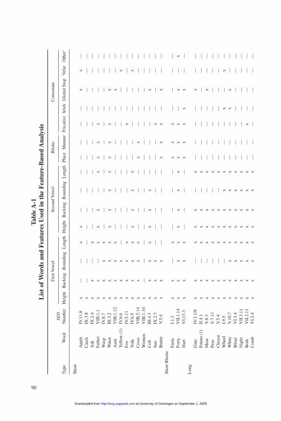
90
Tabl
e A
-1L
ist
of W
ords
and
Fea
ture
s U
sed
in t
he F
eatu
re-B
ased
Ana
lysi
s
Firs
t Vow
elSe
cond
Vow
elR
hotic
Con
sona
ntSE
DTy
peW
ord
Num
ber
Hei
ght
Bac
king
Rou
ndin
gL
engt
hH
eigh
tB
acki
ngR
ound
ing
Len
gth
Plac
eM
anne
rFr
icat
ive
h/w
hG
lotta
l Sto
pV
elar
Oth
er1
Shor
tA
pple
IV.1
1.8
x—
—x
x—
——
——
——
xx
—C
atch
IX.3
.8x
——
——
——
——
——
——
——
Ask
IX.2
.4x
x—
x—
——
——
——
——
——
Fath
erV
III.
1.1
xx
—x
xx
—x
xx
x—
——
—W
asp
IV.8
.7x
xx
x—
——
——
——
——
——
Wat
erII
I.3.
2x
xx
xx
xx
xx
xx
—x
——
Aun
tV
III.
1.12
xx
xx
——
——
——
——
x—
—Y
ello
w (
1)IV
.6.6
xx
x—
——
——
——
——
—x
—Fo
xIV
.5.1
1x
xx
x—
——
——
—x
——
——
Yol
kIV
.6.5
xx
xx
xx
xx
——
——
—x
—C
ross
VII
I.5.
14x
xx
x—
——
—x
x—
——
——
Wom
enV
III.
1.10
x—
——
——
——
——
——
——
—C
olt
III.
4.3
xx
xx
xx
x—
——
——
x—
—Su
nIX
.2.3
xx
x—
——
——
——
x—
——
—B
utte
rV
.5.4
xx
x—
——
——
xx
x—
x—
—Sh
ort R
hotic
Farm
I.1.
3x
x—
x—
——
—x
xx
——
——
Fort
yV
II.1
.14
xx
xx
xx
xx
xx
x—
x—
xH
urt
VI.
13.3
xx
xx
——
——
xx
xx
x—
—L
ong
Gat
eIV
.3.1
/8x
x—
xx
x—
x—
——
—x
——
Pota
to (
1)II
.4.1
xx
—x
xx
—x
——
——
——
—M
eat
V.8
.3x
x—
xx
x—
x—
——
—x
——
Peas
V.7
.13
xx
—x
xx
—x
——
——
——
—C
hees
eV
.5.4
xx
—x
xx
—x
——
——
——
—W
heel
I.9.
5x
x—
xx
xx
x—
——
x—
x—
Whi
teV
.10.
7x
xx
xx
xx
x—
——
xx
——
Blin
dV
I.3.
4x
xx
xx
xx
x—
——
——
——
Nig
htV
II.3
.11
xx
xx
xx
xx
——
——
——
—B
oth
VII
.2.1
1x
xx
xx
xx
x—
—x
——
——
Com
bV
I.2.
4x
xx
xx
xx
x—
——
——
——
at University of Groningen on September 1, 2009 http://eng.sagepub.comDownloaded from
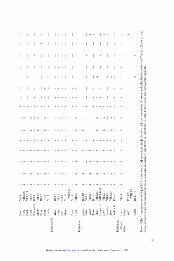
91
Loa
fV
.6.9
xx
xx
xx
xx
——
x—
——
—N
one
VII
.1.1
8x
xx
xx
xx
x—
——
——
——
Col
dV
I.13
.17
xx
xx
xx
xx
——
——
—x
—N
ose
VI.
4.6
xx
xx
xx
xx
——
——
——
—Po
tato
(2)
II.4
.1x
xx
x—
——
—x
xx
—x
——
Moo
nV
II.6
.3x
xx
xx
xx
x—
——
——
——
Woo
lII
I.7.
5x
xx
xx
xx
x—
——
——
xx
Roo
fV
.1.2
xx
xx
xx
xx
xx
——
——
—H
ouse
V.1
.1x
xx
xx
xx
x—
—x
x—
——
Lon
g R
hotic
Mar
eII
I.4.
5x
x—
xx
xx
xx
x—
——
——
Hea
rV
I.4.
2x
x—
xx
xx
xx
x—
x—
——
Fire
V.3
.1x
xx
xx
xx
xx
xx
——
——
Mor
eV
.1.1
7,x
xx
xx
xx
xx
x—
——
——
VII
.8.1
3D
oor
V.1
.8x
xx
xx
xx
xx
x—
——
——
Hou
rV
II.5
.7x
xx
xx
xx
xx
x—
——
——
Dip
htho
ngD
aisy
II.2
.10
xx
—x
xx
—x
——
——
——
—E
ight
VI.
1.7
xx
—x
xx
xx
——
——
x—
—V
oice
VI.
5.17
xx
xx
——
——
——
——
——
xSt
raw
II.8
.2x
xx
xx
xx
xx
x—
——
—x
Tha
wV
II.6
.15
xx
xx
xx
xx
x—
x—
——
—D
augh
ter
VII
I.1.
4/18
xx
xx
xx
xx
xx
x—
x—
—D
ewV
II.6
.7x
xx
xx
xx
x—
——
——
—x
Tue
sday
VII
.4.2
xx
xx
xx
—x
——
——
——
xSn
owV
II.6
.13
xx
xx
xx
xx
——
x—
——
—Y
ello
w (
2)IV
.6.6
xx
xx
xx
——
xx
——
——
—D
ipht
hong
R
hotic
Hai
rV
I.2.
1x
xx
xx
xx
xx
x—
x—
——
Oth
erO
ther
Ver
yIV
.11.
5,—
——
——
——
——
——
——
—x
VII
I.3.
2K
itten
III.
13.1
1—
——
——
——
——
—x
—x
——
Not
e:“O
ther
”co
nson
ants
are
voi
cing
of
[t]
in fo
rty,
loss
of
[w]
in w
ool,
[w]
for
[v]
in v
oice
and
very
,int
rusi
ve [r]
in s
traw
,and
pal
atal
izat
ion
in d
ewan
d Tu
esda
y. Y
ello
w (
1)an
dYe
llow
(2)
refe
r to
the
firs
t and
sec
ond
voca
lic s
egm
ents
,res
pect
ivel
y,an
d Po
tato
(1)
and
Pota
to (
2) r
efer
to th
e se
cond
and
thir
d vo
calic
seg
men
ts.
at University of Groningen on September 1, 2009 http://eng.sagepub.comDownloaded from
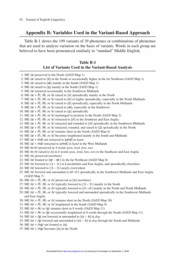
92 Journal of English Linguistics
Appendix B: Variables Used in the Variant-Based Approach
Table B-1 shows the 199 variants of 39 phonemes or combinations of phonemesthat are used to analyze variation on the basis of variants. Words in each group arebelieved to have been pronounced similarly in “standard” Middle English.
Table B-1List of Variants Used in the Variant-Based Analysis
1: ME /a/ preserved in the North (SAED Map 1)2: ME /a/ raised to [E] in the South or occasionally higher in the far Northeast (SAED Map 1)3: ME /a/ raised to [æ] mainly in the South (SAED Map 1)4: ME /a/ raised to [a. ] mainly in the South (SAED Map 1)5: ME /a/ retracted occasionally in the Southwest Midlands6: ME /a/ + /f/, /Q/, or /s/ raised to [«] sporadically mainly in the North 7: ME /a/ + /f/, /Q/, or /s/ raised to [e] or higher sporadically, especially in the North Midlands8: ME /a/ + /f/, /Q/, or /s/ raised to [E] sporadically, especially in the North Midlands9: ME /a/ + /f/, /Q/, or /s/ raised to [æ], especially in the Southwest
10: ME /a/ + /f/, /Q/, or /s/ raised to [a. ] sporadically11: ME /a/ + /f/, /Q/, or /s/ unchanged in position in the North (SAED Map 2)12: ME /a/ + /f/, /Q/, or /s/ retracted to [ ] in the Southeast and East Anglia13: ME /a/ + /f/, /Q/, or /s/ retracted and rounded to [ ] sporadically in the Southwest Midlands14: ME /a/ + /f/, /Q/, or /s/ retracted, rounded, and raised to [O] sporadically in the North15: ME /a/ + /f/, /Q/, or /s/ remains short in the North (SAED Map 4)16: ME /a/ + /f/, /Q/, or /s/ becomes lengthened mainly in the South and Midlands17: ME /a/ + /nd/ not retracted to [ nd] in hand18: ME /a/ + /nd/ retracted to [ nd] in hand in the West Midlands19: ME /e+n/ preserved in 4 words (pen, lend, hen, ten)20: ME /e+n/ raised to [i] in 4 words (pen, lend, hen, ten) in the Southeast and East Anglia 21: ME /o/ preserved (nowhere)22: ME /o/ fronted to [œ ~ œ:] in the far Northeast (SAED Map 8)23: ME /o/ lowered to [O ~ O:] in Lincolnshire and East Anglia, and sporadically elsewhere24: ME /o/ lowered to [O ~ O:] nearly everywhere25: ME /o/ lowered and unrounded to [ ~ :] sporadically in the Southwest Midlands and East Anglia
(SAED Map 7)26: ME /o/ + /f/, /Q/, or /s/ preserved as [o] (nowhere)27: ME /o/ + /f/, /Q/, or /s/ typically lowered to [O ~ O:] mainly in the South28: ME /o/ + /f/, /Q/, or /s/ typically lowered to [ ~ :] mainly in the North and North Midlands29: ME /o/ + /f/, /Q/, or /s/ typically lowered and unrounded sporadically in the Southwest Midlands
and East Anglia30: ME /o/ + /f/, /Q/, or /s/ remains short in the North (SAED Map 10)31: ME /o/ + /f/, /Q/, or /s/ lengthened in the South (SAED Map 9)32: ME /o/ + /k/ or /g/ remains short in 8 words (SAED Map 11)33: ME /o/ + /k/ or /g/ occasionally lengthened in 8 words through the South (SAED Map 11)34: ME /o/ + /g/ not lowered or unrounded to [o ~ U] in dog35: ME /o/ + /g/ lowered and unrounded to [o ~ U] in dog through the South and Midlands36: ME /o/ + /ng/ not fronted to [a]37: ME /o/ + /ng/ becomes [a] in the North
a
aa
a
a a
a a
at University of Groningen on September 1, 2009 http://eng.sagepub.comDownloaded from

Shackleton / Phonetic Variation in Traditional English Dialects 93
Table B-1 (continued)
38: ME /u/ preserved (nowhere)39: ME /u/ shortened to [o ~ o> ] in the Midlands and North (SAED Map 16)40: ME /u/ unrounded to [V] mainly in East Anglia41: ME /u/ fully lowered and unrounded without tenseness to [U] in the Southeast, East Anglia, and
West Midlands42: ME /u/ fully lowered and unrounded with tenseness to [ .U] in the Southwest43: ME /a:/ remains [a:] (nowhere)44: ME /a:/ develops to [i«] in the Northeast (SAED Maps 37 and 37A)45: ME /a:/ develops to [e« ~ E«] in Yorkshire and Lincolnshire (SAED Maps 37 and 37A)46: ME /a:/ develops to [e« ~ E«] in the Midlands (SAED Map 37)47: ME /a:/ develops to [e« ~ E«] in the Southwest (SAED Map 37)48: ME /a:/ develops to [iE ~ jE] in the Northeast (SAED Map 37)49: ME /a:/ develops to [ia ~ ea] in the Northwest (SAED Map 37)50: ME /a:/ develops to [e:] or occasionally [e.:], [eºº:], or [E:] in the North and West (SAED Map 39)51: ME /a:/ develops to [i:] in the Northwest Midlands (SAED Map 40)52: ME /a:/ develops to [ei ~ e:i] through the South (SAED Maps 42 and 45A)53: ME /a:/ develops to [Ei ~ E:i] through the South (SAED Maps 42 and 45A)54: ME /a:/ develops to [æi ~ ai] in the Southeast (SAED Maps 42 and 45A)55: ME /E:/ (< Old English /œ/, /ea/) develops to [i: ~ e:] in the South and Midlands (SAED Map 49)56: ME /E:/ (< Old English /œ/, /ea/) develops to [i: ~ e:] in the far North (SAED Map 49)57: ME /E:/ (< Old English /œ/, /ea/) develops to [Ii] in the South and Midlands (SAED Map 49)58: ME /E:/ (< Old English /œ/, /ea/) develops to [Ii] in the far North (SAED Map 49)59: ME /E:/ (< Old English /œ/, /ea/) develops to [i« ~ e« ~ ju] mainly in the lower North (SAED
Map 50)60: ME /E:/ (< Old English /œ/, /ea/) develops to [Ei] through the South and Midlands (SAED Map 51)61: ME /E:/ (< Old English /œ/, /ea/) develops to [e: ~ E: ~ ei ~ e«] in 8 words through the South and
Midlands (SAED Map 51)62: ME /E:/ (< Old English /œ/, /ea/) develops to [jE] in 7 words sporadically in the West (SAED
Map 52) 63: ME /E:/ (< Old English /œ/, /ea/) develops to [ju ~ jU ~ j«] in 7 words sporadically in the
Southwest Midlands (SAED Map 53)64: ME /E:/ (< Old English /œ/, /ea/) shortened to [E] in the North (SAED Map 54)65: ME /E:/ (< Old English /œ/, /ea/) shortened to [E] in Devonshire (SAED Map 54)66: ME /e:/ preserved (nowhere)67: ME /e:/ typically develops to [i:] nearly everywhere68: ME /e:/ typically develops to [Ii] mainly in the Southeast and East Anglia (SAED Maps 46 and 47)69: ME /e:/ typically develops to [Ii ~ 뺺 i ~ «i] around North Yorkshire (SAED Maps 46 and 47)70: ME /e:/ typically develops to [Ii ~ Ei ~ Ei è] in the Northwest Midlands (SAED Maps 46 and 47)71: ME /e:/ is sporadically shortened to [I] in 9 words in the South (SAED Map 48)72: ME /i:/ preserved (almost nowhere)73: ME /i:/ develops a centered onset in the Southwest (SAED Maps 25 and 26)74: ME /i:/ develops a centered onset in East Anglia (SAED Maps 25 and 26)75: ME /i:/ develops a low-center onset along the southern coast (SAED Maps 21 and 22)76: ME /i:/ develops a low-front or front onset in the North (SAED Maps 21 and 22)77: ME /i:/ develops a low-front or front onset in Shropshire and occasionally in the Midlands (SAED
Maps 21 and 22) 78: ME /i:/ develops a low-front or front onset in the Southwest (SAED Maps 21 and 22)
(continued)
at University of Groningen on September 1, 2009 http://eng.sagepub.comDownloaded from
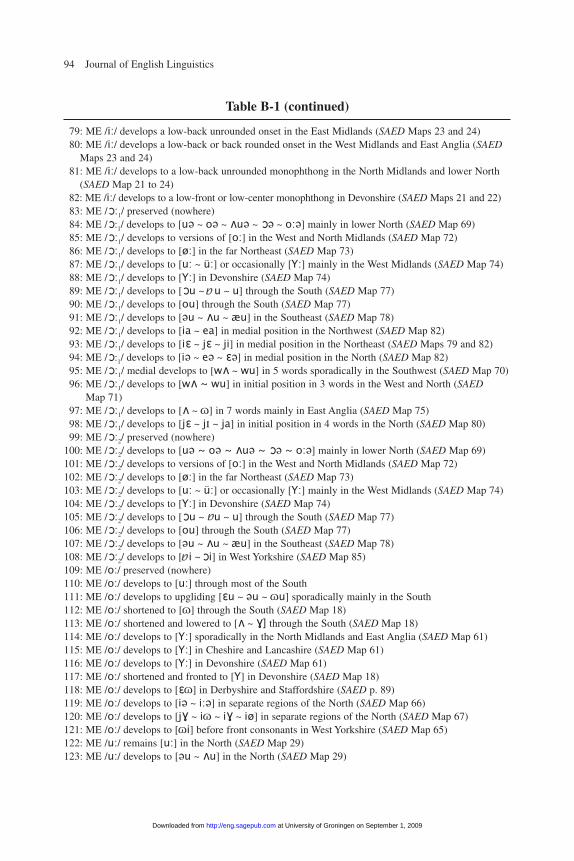
94 Journal of English Linguistics
Table B-1 (continued)
79: ME /i:/ develops a low-back unrounded onset in the East Midlands (SAED Maps 23 and 24)80: ME /i:/ develops a low-back or back rounded onset in the West Midlands and East Anglia (SAED
Maps 23 and 24)81: ME /i:/ develops to a low-back unrounded monophthong in the North Midlands and lower North
(SAED Map 21 to 24)82: ME /i:/ develops to a low-front or low-center monophthong in Devonshire (SAED Maps 21 and 22) 83: ME /O:1/ preserved (nowhere)84: ME /O:1/ develops to [u« ~ o« ~ Uu« ~ O« ~ o:«] mainly in lower North (SAED Map 69)85: ME /O:1/ develops to versions of [o:] in the West and North Midlands (SAED Map 72)86: ME /O:1/ develops to [ø:] in the far Northeast (SAED Map 73)87: ME /O:1/ develops to [u: ~ ü:] or occasionally [Y:] mainly in the West Midlands (SAED Map 74)88: ME /O:1/ develops to [Y:] in Devonshire (SAED Map 74)89: ME /O:1/ develops to [Ou ~ u ~ u] through the South (SAED Map 77)90: ME /O:1/ develops to [ou] through the South (SAED Map 77)91: ME /O:1/ develops to [«u ~ Uu ~ æu] in the Southeast (SAED Map 78)92: ME /O:1/ develops to [ia ~ ea] in medial position in the Northwest (SAED Map 82)93: ME /O:1/ develops to [iE ~ jE ~ ji] in medial position in the Northeast (SAED Maps 79 and 82)94: ME /O:1/ develops to [i« ~ e« ~ E«] in medial position in the North (SAED Map 82)95: ME /O:1/ medial develops to [wU ~ wu] in 5 words sporadically in the Southwest (SAED Map 70)96: ME /O:1/ develops to [wU ~ wu] in initial position in 3 words in the West and North (SAED
Map 71)97: ME /O:1/ develops to [U ~ o] in 7 words mainly in East Anglia (SAED Map 75)98: ME /O:1/ develops to [jE ~ jI ~ ja] in initial position in 4 words in the North (SAED Map 80)99: ME /O:2/ preserved (nowhere)
100: ME /O:2/ develops to [u« ~ o« ~ Uu« ~ O« ~ o:«] mainly in lower North (SAED Map 69)101: ME /O:2/ develops to versions of [o:] in the West and North Midlands (SAED Map 72)102: ME /O:2/ develops to [ø:] in the far Northeast (SAED Map 73)103: ME /O:2/ develops to [u: ~ ü:] or occasionally [Y:] mainly in the West Midlands (SAED Map 74)104: ME /O:2/ develops to [Y:] in Devonshire (SAED Map 74)105: ME /O:2/ develops to [Ou ~ u ~ u] through the South (SAED Map 77)106: ME /O:2/ develops to [ou] through the South (SAED Map 77)107: ME /O:2/ develops to [«u ~ Uu ~ æu] in the Southeast (SAED Map 78)108: ME /O:2/ develops to [ i ~Oi] in West Yorkshire (SAED Map 85)109: ME /o:/ preserved (nowhere)110: ME /o:/ develops to [u:] through most of the South111: ME /o:/ develops to upgliding [Eu ~ «u ~ ou] sporadically mainly in the South112: ME /o:/ shortened to [o] through the South (SAED Map 18)113: ME /o:/ shortened and lowered to [U ~ V] through the South (SAED Map 18)114: ME /o:/ develops to [Y:] sporadically in the North Midlands and East Anglia (SAED Map 61)115: ME /o:/ develops to [Y:] in Cheshire and Lancashire (SAED Map 61)116: ME /o:/ develops to [Y:] in Devonshire (SAED Map 61)117: ME /o:/ shortened and fronted to [Y] in Devonshire (SAED Map 18)118: ME /o:/ develops to [Eo] in Derbyshire and Staffordshire (SAED p. 89) 119: ME /o:/ develops to [i« ~ i:«] in separate regions of the North (SAED Map 66)120: ME /o:/ develops to [jV ~ io ~ iV ~ iø] in separate regions of the North (SAED Map 67)121: ME /o:/ develops to [oi] before front consonants in West Yorkshire (SAED Map 65)122: ME /u:/ remains [u:] in the North (SAED Map 29)123: ME /u:/ develops to [«u ~ Uu] in the North (SAED Map 29)
a
a
a
at University of Groningen on September 1, 2009 http://eng.sagepub.comDownloaded from
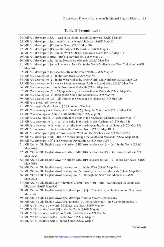
Shackleton / Phonetic Variation in Traditional English Dialects 95
Table B-1 (continued)
124: ME /u:/ develops to [«u ~ Uu] in the South, mainly Southwest (SAED Map 29)125: ME /u:/ develops to [æu] mainly in the North Midlands (SAED Map 30)126: ME /u:/ develops to [Eu] in the South (SAED Map 30)127: ME /u:/ develops to [EY] on the edges of Devonshire (SAED Map 30)128: ME /u:/ develops to [au] in the West Midlands and lower North (SAED Map 31)129: ME /u:/ develops to [œu ~ œY] in Devonshire (SAED Map 32)130: ME /u:/ develops to [ai] in the Northwest Midlands (SAED Map 33)131: ME /u:/ develops to [æ: ~ E: ~ æ« ~ E« ~ Ea] in the North Midlands and West Yorkshire (SAED
Map 34)132: ME /u:/ develops to [a:] sporadically in the lower North (SAED Map 35)133: ME /ai/ develops to [E:] in the Northwest (SAED Map 92)134: ME /ai/ develops to [e:] in the West Midlands, lower North, and Northeast (SAED Map 92)135: ME /ai/ develops to [E« ~ e« ~ i«] in the eastern North to Lincolnshire (SAED Map 93)136: ME /ai/ develops to [i:] in the Northwest Midlands (SAED Map 94)137: ME /ai/ develops to [ei ~ e:i] sporadically in the South and Midlands (SAED Map 95)138: ME /ai/ develops to [Ei] through the South and Midlands (SAED Map 95)139: ME /ai/ develops to [æi ~ ai] through the South and Midlands (SAED Map 95)140: ME /au/ preserved (nowhere)141: ME /au/ typically develops to [O:] in most of England142: ME /au/ develops to a closer, more rounded ºO:] along the South coast (SAED Map 13)143: ME /au/ develops to [oo] in north Staffordshire (SAED p. 21)144: ME /au/ develops to [ :] especially in 6 words in the Southwest Midlands (SAED Map 13)145: ME /au/ develops to [a: ~ æ:] especially in 6 words in the Northeast (SAED Map 14)146: ME /au/ develops to [a: ~ æ:] especially in 6 words sporadically in the South (SAED Map 14)147: ME /iu/ remains [iu] in 5 words in the East and North (SAED Map 100A)148: ME /iu/ develops to [ju] in 5 words in the West and the Northeast (SAED Map 100A)149: ME /iu/ develops to [u: ~ ü:] in 5 words through the South and Midlands (SAED Map 100B) 150: ME /iu/ develops to [Y:] in 5 words in Devonshire (SAED Map 100B)151: ME /Ou/ (< Old English /aw/ = Northern ME /au/) develops to [O: ~ O:«] in the North (SAED
Map 96A)152: ME /Ou/ (< Old English /aw/ = Northern ME /au/) develops to [a:] in the lower North (SAED
Map 96A)153: ME /Ou/ (< Old English /aw/ = Northern ME /au/) develops to [œ: ~ ø:] in the Northeast (SAED
Map 96B)154: ME /Ou/ (< Old English /aw/) develops to [o:] in the West (SAED Map 96B)155: ME /Ou/ (< Old English /aw/) develops to [Ou] mainly in the East Midlands (SAED Map 96C)156: ME /Ou/ (< Old English /aw/) develops to [ou] through the South and Midlands (SAED
Map 96C)157: ME /Ou/ (< Old English /aw/) develops to [Uu ~ u ~ au ~ æu ~ Eu] through the South and
Midlands (SAED Map 96C)158: ME /Ou/ (< Old English /aw/) final develops to [e] in 5 words in the Southwest and Southwest
Midlands159: ME /Ou/ (< Old English /aw/) final develops to [«] in 5 words sporadically160: ME /Ou/ (< Old English /aw/) final remains [ou] or develops to [I] in 5 words sporadically161: ME /ar/ [r] lost in the North, Midlands, and East (SAED Map 6)162: ME /ar/ [r] retained with [R] in the far North (SAED Map 6)163: ME /ar/ [r] retained with [r] in North Cumberland (SAED Map 6)164: ME /ar/ [r] retained with [»] in the North (SAED Map 6)165: ME /ar/ [r] retained with [»] in the South (SAED Map 6)
(continued)
a
a
at University of Groningen on September 1, 2009 http://eng.sagepub.comDownloaded from
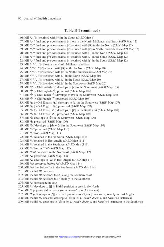
96 Journal of English Linguistics
Table B-1 (continued)
166: ME /ar/ [r] retained with [r] in the South (SAED Map 6)167: ME /or/ final and pre-consonantal [r] lost in the North, Midlands, and East (SAED Map 12)168: ME /or/ final and pre-consonantal [r] retained with [R] in the far North (SAED Map 12)169: ME /or/ final and pre-consonantal [r] retained with [r] in North Cumberland (SAED Map 12)170: ME /or/ final and pre-consonantal [r] retained with [»] in the North (SAED Map 12)171: ME /or/ final and pre-consonantal [r] retained with [»] in the South (SAED Map 12)172: ME /or/ final and pre-consonantal [r] retained with [r] in the South (SAED Map 12)173: ME /ir/-/ur/ [r] lost in the North, Midlands, and East174: ME /ir/-/ur/ [r] retained with [R] in the far North (SAED Map 20)175: ME /ir/-/ur/ [r] retained with [r] in North Cumberland (SAED Map 20)176: ME /ir/-/ur/ [r] retained with [»] in the North (SAED Map 20)177: ME /ir/-/ur/ [r] retained with [»] in the South (SAED Map 20)178: ME /ir/-/ur/ [r] retained with [r] in the Southwest (SAED Map 20)179: ME /f/ (> Old English /f/) develops to [v] in the Southwest (SAED Map 105)180: ME /f/ (> Old English /f/) preserved (SAED Map 105)181: ME /f/ (> Old French /f/) develops to [v] in the Southwest (SAED Map 106)182: ME /f/ (> Old French /f/) preserved (SAED Map 106)183: ME /s/ (> Old English /s/) develops to [z] in the Southwest (SAED Map 107)184: ME /s/ (> Old English /s/) preserved (SAED Map 107)185: ME /s/ (> Old French /s/) develops to [z] in the Southwest (SAED Map 108)186: ME /s/ (> Old French /s/) preserved (SAED Map 108)187: ME /Q/ develops to [ð] in the Southwest (SAED Map 109)188: ME /Q/ preserved (SAED Map 109)189: ME /Qr/ develops to [dr ~ ðr] in the Southwest (SAED Map 110)190: ME /Qr/ preserved (SAED Map 110)191: ME /h/ lost (SAED Map 111)192: ME /h/ retained in the far North (SAED Map (111)193: ME /h/ retained in East Anglia (SAED Map (111)194: ME /h/ retained in the Southwest (SAED Map (111)195: ME /h/ lost in /hw/ (SAED Map 112)196: ME /hw/ preserved in the Northeast (SAED Map 112)197: ME /v/ preserved (SAED Map 113)198: ME /v/ develops to [w] in East Anglia (SAED Map 113)199: ME /w/ preserved before /u/ (SAED Map 114)200: ME /w/ lost before /u/ in the Southwest (SAED Map 114)201: ME medial /t/ preserved202: ME medial /t/ develops to [d] along the southern coast203: ME medial /t/ develops to [?] mainly in the Southeast204: ME /g/ unchanged in gate205: ME /g/ develops to [j] in initial position in gate in the North206: ME /t y/ preserved in aren’t you or weren’t you (3 instances)207: ME /t y/ develops to [tS] in aren’t you or weren’t you (3 instances) mainly in East Anglia208: ME medial /s/ does not develop to [d] in isn’t, wasn’t, doesn’t, and hasn’t (4 instances)209: ME medial /s/ develops to [d] in isn’t, wasn’t, doesn’t, and hasn’t (4 instances) in the Southwest
at University of Groningen on September 1, 2009 http://eng.sagepub.comDownloaded from
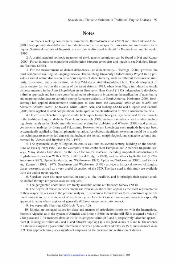
Shackleton / Phonetic Variation in Traditional English Dialects 97
Notes
1. For readers seeking non-technical summaries, Bartholemew et al. (2002) and Tabachnik and Fidell(2000) both provide straightforward introductions to the use of specific univariate and multivariate tech-niques. Statistical analysis of linguistic survey data is discussed in detail by Kretzschmar and Schneider(1996).
2. A useful standard textbook treatment of phylogenetic techniques can be found in Nei and Kumar(2000). For an interesting example of collaboration between geneticists and linguists, see Nakhleh, Ringe,and Warnow (2005).
3. For the measurement of dialect differences—or dialectometry—Heeringa (2004) provides themost comprehensive English-language review. The Salzburg University Dialectometry Project (n.d.) pro-vides a useful online discussion of various aspects of dialectometry, such as different measures of simi-larity, dispersion, and classification, at http://ald.sbg.ac.at/dm/Engl/default.htm. The development ofdialectometry (as well as the coining of the term) dates to 1973, when Jean Séguy introduced a simpledistance measure in the Atlas Linguistique de la Gascogne. Hans Goebl (1982) independently developeda similar approach and has since contributed major advances in broadening the application of quantitativeand mapping techniques to variation among Romance dialects. In North America, Nerbonne (2006, forth-coming) has applied dialectometric techniques to data from the Linguistic Atlas of the Middle andSouthern Atlantic States (LAMSAS), while Labov, Ash, and Boberg (2006) and Clopper and Paolillo(2006) have applied related computational techniques in the classification of North American dialects.
4. Other researchers have applied similar techniques to morphological, syntactic, and lexical variantsin the traditional English dialects. Viereck and Ramisch (1997) include a number of such studies, includ-ing cluster analyses by Goebl, multidimensional scaling by Embleton and Wheeler (1997), and principalcomponents analyses by Inoue and Fukoshima. However, to my knowledge such methods have not beensystematically applied to English phonetic variation. An obvious significant extension would be to applythe techniques to an extended data set that includes the lexical, morphological, and syntactic variants enu-merated by Viereck and Ramisch (1991, 1997).
5. The systematic study of English dialects is well into its second century, building on the founda-tions of Ellis ([1889] 1968) and the examples of the continental European and American linguistic sur-veys. Many studies have drawn on the SED for source material, including important introductions toEnglish dialects such as Wells (1982a, 1982b) and Trudgill (1999); and the atlases by Kolb et al. (1979),Anderson (1987), Upton, Sanderson, and Widdowson (1987), Upton and Widdowson (1996), and Viereckand Ramisch (1991, 1997). Sanderson and Widdowson (1985) provide a historical review of Englishdialect research, as well as a very useful discussion of the SED. The data used in this study are availablefrom the author upon request.
6. Speakers were also tape-recorded in nearly all the localities, and in principle their speech couldbe studied through a rigorous acoustic analysis.
7. The geographic coordinates are freely available online at Ordnance Survey (2006).8. The degree of variation bears emphasis: even in localities that appear as the most representative
of their respective regions in the present analysis, it is common to find two or three sometimes quite dif-ferent variants in use in a given set of words in a given locality. Competition among variants is especiallyapparent in areas where regions of generally different usage come into contact.
9. See especially Heeringa (2004, ch. 7, sec. 4.3).10. Rhotics are assigned values for place and manner of articulation consistent with the International
Phonetic Alphabet as in the system of Almeida and Braun (1986): the uvular trill [R] is assigned a value of9 for place and 3 for manner; alveolar trill [r] is assigned values of 3 and 4, respectively; alveolar approxi-mant [r] is assigned values of 7 and 4; and retroflex tap/flap [®] is assigned values of 4 and 6. The absenceof a rhotic is assigned a place value intermediate between postalveolar and retroflex (5.5) and a manner valueof 9. This approach thus places significant emphasis on the presence and realization of rhotics.
at University of Groningen on September 1, 2009 http://eng.sagepub.comDownloaded from

98 Journal of English Linguistics
11. The addition of standard Middle English also requires the addition of 10 variants that were nolonger in use in any of the localities under study in the twentieth century; the variants identified forReceived Pronunciation and Western Reserve were all in use in at least a few localities.
12. Because the maps present only ranges of frequencies, I use the averages of those ranges (i.e., 92.5percent for speakers with frequencies between 85 percent and 100 percent). That approach also requiresthat each locality’s frequencies be normalized to sum to 1.0 over each set of words that are held to sharea phoneme in Middle English (since they may not do so automatically) and introduces a layer of error tothe data that should be of relatively little consequence for the analysis.
13. See for example Trudgill (1999, 41). Trudgill attributes this characterization to the speech of allof Staffordshire plus parts of Cheshire, Shropshire, Derbyshire, Warwickshire, and Worcestershire.
14. First introduced into dialectology by Kessler (1995) to measure dialect distances among speakersof Irish Gaelic, the Levenshtein distance has become a preferred approach for many researchers becauseof its comprehensiveness and flexibility.
15. The distance measures are calculated using Fortran-based programs developed by and availablefrom the author upon request.
16. Goebl and Schiltz (1997) extend the analysis of skewness for SED localities on the basis of lexicaland morphological characteristics, showing that localities with the same average similarity with other locali-ties may differ in the distribution of distances from low values to high values, so that one is relatively similarto most other localities but very different from a few, while the other is somewhat dissimilar to most but notterribly similar to any. They show that for the linguistic variables they examine, a swath of south-centralEngland has the lowest degree of skewness and thus the greatest degree of integration into the dialect contin-uum. In the present study, in contrast, the lowest degree of skewness for localities’ linguistic distances occursin the Midlands, mainly but not invariably among those localities that have the lowest average distances.
17. Interestingly, regional American informants analyzed in Shackleton (2005) had an average lin-guistic distance from Lowman’s southern English informants of about 1.18, while the average distanceamong the English informants was about 1.00. For the SED localities in the same geographic region asLowman’s informants, the average variant-based linguistic distance with Western Reserve speech is about1.23, while the average distance among the SED localities is about 1.08. Despite the fact that the two stud-ies measure pronunciations of different variants by different informants, they yield fairly similar rangesof similarity among speakers in southern England and between those speakers and American speakers,tending to corroborate these comparisons of synchronic and diachronic distance. However, the compari-son between linguistic distances measured from Lowman’s data and those measured from SED dataobtains only for the full data sets and breaks down at the county level.
18. The importance of rhoticity as the source of this difference in patterns becomes evident when onecompares the patterns of similarity between the two speech forms and those of the SED localities. Usingthe variant-based linguistic measure, Received Pronunciation and Western Reserve have very similar pat-terns of distance with SED localities, such that their patterns have a correlation coefficient of 0.84. Usingthe feature-based measure, their patterns remain similar except that Western Reserve’s distances with thefully rhotic localities of the Southwest are all rather uniformly shifted lower, compared with ReceivedPronunciation. As a result of that shift, the two patterns become slightly negatively correlated.
19. Bartholomew et al. (2002, ch. 2) provides a clear introduction to cluster techniques, including anillustration involving Midlands data from the SED. Romesburg (2004) provides a more detailed overviewof cluster analytic techniques, as well as a clear discussion of the strengths and weaknesses of differentalgorithms.
20. Kleinberg (2003) shows that no clustering method can simultaneously achieve three simple, desir-able properties (scale invariance, consistency, and richness), and that every method involves unavoidabletrade-offs among these desirable properties.
21. Rug/L04 (n.d.) is freely available online at http://www.let.rug.nl/~kleiweg/indexs.html.22. PHYLIP (2006) is freely available online at http://evolution.genetics.washington.edu/phylip.html.
at University of Groningen on September 1, 2009 http://eng.sagepub.comDownloaded from
Shackleton / Phonetic Variation in Traditional English Dialects 99
23. Both Kruskal and Wish (1978) and Bartholomew et al. (2002, ch. 3) provide straightforward intro-ductions to multidimensional scaling.
24. The polygons in these maps represent individual localities, each of which is located in the middleof its polygon.
25. Similar maps in Viereck (1985) showing lexical and morphological distances reveal similar patterns.26. See Tabachnick and Fidell (2000, ch. 5) for an overview of multiple regression analysis.27. SPSS is available at http://www.spss.com (SPSS 2006).28. That approach is consistent with the observation that increasing distance tends to have a decreas-
ing incremental influence on linguistic differences.29. The negative value of the parameter for “Dummy, Regions 5 and 5” in the variant-based regres-
sion has no realistic interpretation, but it indicates that localities in Lincolnshire are much more similarto each other than is typical in most regions of England. The insignificant values for four intraregionaldummies imply that the effect of geographic distance on intraregional linguistic differences in thoseregions cannot be distinguished from its effect on such differences in the Far North.
30. Barrier Version 2.2 is freely available online at http://www.mnhn.fr/mnhn/ecoanthropologie/soft-ware/barrier.html (Barrier 2006).
31. Tabachnick and Fidell (2000, ch. 1) provide an introduction to principal components analysis, as doBartholomew et al. (2002, ch. 5). Several recent studies have applied principal components analysis or theclosely related factor analysis to linguistic data, including Labov, Ash, and Boberg’s (2006) and Clopper andPaolillo’s (2006) analyses of acoustic features of North American English; Nerbonne’s (2006) analyses ofvariation in Middle and Southern Atlantic American English; and Shackleton’s (2005) examination of usagedifferences among speakers of various English and American dialects. As noted by Nerbonne, an argumentcan be made that principal components analysis, which is essentially an exploratory technique, is less prefer-able to use for the present analysis than factor analysis, which is more appropriate when the aim of the analy-sis is to uncover underlying structures—or “latent variables”—that are manifested in the variables underanalysis. However, factor analysis requires a matrix of variables in which none of the rows is a linear com-bination of the others, which for the variant-based analysis requires that localities’ frequencies of the vari-ous pronunciations of a given set of words cannot sum to 100 percent. Moreover, principal componentsanalysis and factor analysis typically yield very similar results, so the advantages of being able to examineall pronunciations in the data would appear to outweigh the advantage of being able to rigorously uncoverlatent variables.
32. SAS/STAT is available at http://www.sas.com/technologies/analytics/statistics/stat/index.html(SAS 2006).
33. The recommendation is generally phrased in terms of highest eigenvalues rather than highestexplanatory value. The widely recommended practice of retaining principal components with eigenvaluesgreater than 1.0 is among the least accurate of methods. See Costello and Osborne (2005).
34. Labov, Ash, and Boberg (2006) apply principal components analysis (PCA) to acoustic data—specifically, to formant data—in their classification of North American dialects; and Clopper and Paolillo(2006) identify systematic phonetic shifts in the American North and South by applying the related factoranalysis approach to acoustic data. To my knowledge, however, the present study is the first to apply PCAto features.
35. The historical origins of voicing of initial fricatives are poorly understood and, as voicing is foundin Germanic dialects on the continent, may even extend to the earliest period of Anglo-Saxon settlementin England. Whatever the case may be, it appears likely that voicing prevailed over much of southernEngland, including most localities south of a line extending from mid-Shropshire to the Suffolk-Essexborder, until as late as the 17th century and may not have become considerably more restricted until theonset of industrialization in the early 19th century. See Voitl (1988).
36. Parenthetically, American researchers may find it particularly noteworthy that the southeast coastappears to be the only region in England in which localities’ long vowels /a:/, /E:/~/e:/, /i:/, /O:1/~/O:2/, /o:/,
at University of Groningen on September 1, 2009 http://eng.sagepub.comDownloaded from
100 Journal of English Linguistics
and /u:/ tend to develop forms approaching [Ei], [Ii], [ i], [ou], [Ou], and [Eu], respectively. Consideredalong with the tendencies to raise the front short vowels and to retain rhoticity after vowels, the systemof diphthongs appears to point to the Southeast as the probable source of the rather similar system in muchof America, particularly in the South.
37. Taken as a whole, the Central Midlands are also noticeably congruent with the area that Glauser(1985) identifies as having only imperfectly undergone the backing and rounding of /wa/.
References
Almeida, A., and A. Braun. 1986. “Richtig” und “Falsch” in phonetischer Transkription; Vorschläge zumVergleigh von Transkriptionen mit Beispielen aus deutschen Dialekten. Zeitschrift für Dialektologieund Linguistik 53 (2): 158-72.
Anderson, Peter M. 1987. A structural atlas of the English dialects. London: Croom Helm.Bartholomew, David J., Fiona Steele, Irini Moustaki, and Jane I. Galbraith. 2002. The analysis and inter-
pretation of multivariate data for social scientists. New York: Chapman & Hall/CRC. Clopper, Cynthia G., and John C. Paolillo. 2006. North American English vowels: A factor-analytic per-
spective. Literary and Linguistic Computing 21 (4): 445-62.Costello, Anna B., and Jason W. Osborne. 2005. Best practices in exploratory factor analysis: Four recom-
mendations for getting the most from your analysis. Practical Assessment, Research & Evaluation 10(7): 1-9.
Ellis, Alexander J. [1889] 1968. On early English pronunciation, part V: The existing phonology ofEnglish dialects compared with that of West Saxon speech. New York: Greenwood. (Originally pub-lished by Asher & Co., London.)
Embleton, Sheila, and Eric Wheeler. 1997. Multidimensional scaling and the SED data. In computerdeveloped linguistic atlas of England (CLAE), vol. 2, edited by Wolfgang Viereck and HeinrichRamisch, 5-11. Tübingen, Germany: Max Niemeyer Verlag.
Glauser, Beat. 1985. Linguistic atlases and generative phonology. In Studies in linguistic geography: Thedialects of English in Britain and Ireland, edited by John M. Kirk, Stewart Sanderson, and J. D. A.Widdowson, 113-29. London: Croom Helm.
Goebl, Hans. 1982. Dialektometrie. Prinzipien und Methoden des Einsatzes der Numerischen Taxonomieim Bereich der Dialektgeographie. Vienna: Denkschriften der Österreichischen Akademie derWissenschaften, phil.-hist. Klasse, Band 157.
———. 1997. Some dendrographic classifications of the data of CLAE 1 and CLAE 2. In Computerdeveloped linguistic atlas of England (CLAE), vol. 2, edited by Wolfgang Viereck and HeinrichRamisch, 23-32. Tübingen, Germany: Max Niemeyer Verlag.
Goebl, Hans, and Guillaume Schiltz. 1997. A dialectometrical compilation of CLAE 1 and CLAE 2:Isoglosses and dialect integration. In Computer developed linguistic atlas of England (CLAE), vol. 2,edited by Wolfgang Viereck and Heinrich Ramisch, 13-21. Tübingen, Germany: Max Niemeyer Verlag.
Händler, Harald, and Wolfgang Viereck. 1997. Selective dialectometry. In Computer developed linguisticatlas of England (CLAE), vol. 2, edited by Wolfgang Viereck and Heinrich Ramisch, 33-49. Tübingen,Germany: Max Niemeyer Verlag.
Heeringa, Wilbert. 2004. Measuring dialect pronunciation differences using Levenshtein distance.Groningen Dissertations in Linguistics 46. Groningen, Netherlands: University of Groningen.
Inoue, Fumio, and Chitsuko Fukushima. 1997. A quantitative approach to English dialect distribution:Analyses of CLAE morphological data. In Computer developed linguistic atlas of England (CLAE), vol.2, edited by Wolfgang Viereck and Heinrich Ramisch, 57-65. Tübingen, Germany: Max Niemeyer Verlag.
Kessler, Brett. 1995. Computational dialectology in Irish Gaelic. In Proceedings of the EuropeanAssociation for Computational Linguistics, 60-67. Dublin: EACL.
a
at University of Groningen on September 1, 2009 http://eng.sagepub.comDownloaded from

Shackleton / Phonetic Variation in Traditional English Dialects 101
Kleinberg, Jon. 2003. An impossibility theorem for clustering. In Advances in neural information pro-cessing systems 15: Proceedings of the 15th Conference on Neural Information Processing Systems,200, edited by Suzanna Becker, Sebastian Thrun, and Klaus Obermayer. Cambridge, MA: MIT Press.http://books.nips.cc/papers/files/nips15/LT17.pdf (accessed December 18, 2006).
Kolb, Eduard, Beat Glauser, Willy Elmer, and Renate Stamm. 1979. Atlas of English sounds. Bern:Francke.
Kretzschmar, William A., and Edgar Schneider. 1996. Introduction to quantitative analysis of linguisticsurvey data: An atlas by the numbers. Thousand Oaks, CA: Sage.
Kretzschmar, William A., and Susan Tamasi. 2002. Distributional foundations for a theory of languagechange. World Englishes 22 (4): 377-401.
Kruskal, Joseph B., and Myron Wish. 1978. Multidimensional scaling. Thousand Oaks, CA: Sage.Labov, William, Sharon Ash, and Charles Boberg. 2006. Atlas of North American English. New York:
DeGruyter.Manni, Franz, and Italo Barrai. 2001. Genetic structures and linguistic boundaries in Italy: A microre-
gional approach. Human Biology 73 (3): 335-48.Manni, F., E. Guérard, and E. Heyer. 2004. Geographic patterns of (genetic, morphologic, linguistic) vari-
ation: how barriers can be detected by “Monmonier’s algorithm.” Human Biology 76 (2): 173-90.Monmonier, Mark. 1973. Maximum-difference barriers: An alternative numerical regionalization method.
Geographical Analysis 3:245-61. Nakhleh, Luay, Don Ringe, and Tandy Warnow. 2005. Perfect phylogenetic networks: A new methodol-
ogy for reconstructing the evolutionary history of natural languages. Language 81 (2): 382-420.Nei, Masatoshi, and Sudhir Kumar. 2000. Molecular evolution and phylogenetics. Oxford: Oxford
University Press.Nerbonne, John. 2006. Identifying linguistic structure in aggregate comparison. Literary and Linguistic
Computing 21 (4): 463-76.———. Forthcoming. Various variation aggregates in the LAMSAS South. In Language variety in the
South III, edited by Catherine Davis and Michael Picone. Tuscaloosa: University of Alabama Press.Ordnance Survey. 2006. Did you know . . . ? http://www.ordnancesurvey.co.uk/oswebsite/freefun/
didyouknow/ (accessed December 18, 2006).Orton, Harold, and Eugen Dieth, eds. 1962. Survey of English dialects. Leeds, UK: E. J. Arnold.PHYLIP. 2006. Phylip. http://evolution.genetics.washington.edu/phylip.html (accessed December 18,
2006).Romesburg, Charles. 2004. Cluster analysis for researchers. Morrisville, NC: Lulu Press.Rug/L04. N.d. Rug/L04 software for dialectometrics and cartography. http://www.let.rug.nl/~kleiweg/
indexs.html (accessed December 18, 2006).Sanderson, Stewart, and J. D. A. Widdowson. 1985. Linguistic geography in England: Progress and
prospects. In Studies in linguistic geography: The dialects of English in Britain and Ireland, edited byJohn M. Kirk, Stewart Sanderson, and J. D. A. Widdowson, 34-50. London: Croom Helm.
Salzburg University Dialectometry Project. N.d. Dialectometry Project: Salzburg University. http://ald.sbg.ac.at/dm/Engl/default.htm (accessed December 18, 2006).
SAS. 2006. SAS/STAT. http://www.sas.com/technologies/analytics/statistics/stat/index.html (accessedDecember 18, 2006).
Séguy, Jean. 1973. Atlas Linguistique de la Gascogne. Paris: Centre National de la Recherche Scientifique.Shackleton, Robert G., Jr. 2005. English-American speech relationships: A quantitative approach. Journal
of English Linguistics 33 (2): 99-160.SPSS. 2006. SPSS for Windows, v. 7.5. http://www.spss.com (accessed December 18, 2006).Tabachnick, Barbara G., and Linda S. Fidell. 2000. Using multivariate statistics. Boston: Allyn & Bacon.Trudgill, Peter. 1999. The dialects of England. 2nd rev. ed. Oxford: Blackwell.Upton, Clive, Stewart Sanderson, and John Widdowson. 1987. Word maps: Dialect atlas of England. New
York: Routledge.
at University of Groningen on September 1, 2009 http://eng.sagepub.comDownloaded from
102 Journal of English Linguistics
Upton, Clive, and John Widdowson. 1996. An atlas of English dialects. Oxford: Oxford University Press.Viereck, Wolfgang. 1985. Linguistic atlases and dialectometry: The survey of English dialects. In Studies in
linguistic geography: The dialects of English in Britain and Ireland, edited by John M. Kirk, StewartSanderson, and J. D. A. Widdowson, 94-112. London: Croom Helm.
Viereck, Wolfgang, and Heinrich Ramisch, eds. 1991. Computer developed linguistic atlas of England(CLAE), vol. 1. Tübingen, Germany: Max Niemeyer Verlag.
———, eds. 1997. Computer developed linguistic atlas of England (CLAE), vol. 2. Tübingen, Germany:Max Niemeyer Verlag.
Voitl, Herbert. 1988. The history of voicing of initial fricatives in Southern England: A case of conflictbetween regional and social dialect. In Historical dialectology: Regional and social, edited by JacekFisiak, 555-600. Trends in Linguistics, Studies and Monographs 37. New York: Mouton de Gruyter.
Wells, J. C. 1982a. Accents of English 1: An introduction. Cambridge: Cambridge University Press.———. 1982b. Accents of English 2: The British Isles. Cambridge: Cambridge University Press.
Robert G. Shackleton Jr. is a principal analyst in the Macroeconomic Analysis Division of theCongressional Budget Office in Washington, D.C. His principal areas of research are the economics ofclimate change, the international macroeconomic implications of the global demographic transition, andretirement preparations among baby boomers. His area of interest in linguistic research is the quantifica-tion of dialect variation, especially as it bears on the origin and diffusion of American dialect features.
at University of Groningen on September 1, 2009 http://eng.sagepub.comDownloaded from