Journal of Development Economics 132 (2018) 130–149

Contents lists available at ScienceDirect

Journal of Development Economics

journal homepage: www.elsevier.com/locate/devec

Using spatial factor analysis to measure human development

Qihua Qiu a,*, Jaesang Sung a, Will Davis a, Rusty Tchernis a,b

a Department of Economics, Georgia State University, USAb IZA & NBER, USA

A R T I C L E I N F O

JEL classification:O15O57

Keywords:Human development indexFactor analysis

* Corresponding author. Department of Economics, GeoE-mail address: jessica.qqh@gmail.com (Q. Qiu).

1 For a more detailed account of the rationale behind t2 For instance, the relationship between the HDI and h

depressive episodes (Cifuentes et al., 2008), kidney canceret al., 2011).

https://doi.org/10.1016/j.jdeveco.2017.12.007Received 19 August 2016; Received in revised form 26 OAvailable online 28 December 20170304-3878/© 2017 Elsevier B.V. All rights reserved.

A B S T R A C T

We propose a Bayesian factor analysis model as an alternative to the Human Development Index (HDI). Our modelprovides methodology which can either augment or build additional indices. In addition to addressing potentialissues of the HDI, we estimate human development with three auxiliary variables capturing environmental healthand sustainability, income inequality, and satellite observed nightlight. We also use our method to build a Mil-lennium Development Goals (MDG) index as an example of constructing a more complex index. We find the“living standard” dimension provides a greater contribution to human development than the official HDI suggests,while the “longevity” dimension provides a lower proportional contribution. Our results also show considerablelevels of disagreement relative to the ranks of official HDI. We report the sensitivity of our method to differentspecifications of spatial correlation, cardinal-to-ordinal data transforms, and data imputation procedures, alongwith the results of a simulated data exercise.

1. Introduction

Designed as a ranking system to track global human development, theHuman Development Index (HDI) was first introduced in 1990 by theUnited Nations Development Programme (UNDP) in their now annualseries of annual Human Development Reports (HDR's). Prior to the HDI'sinitial publication, GDP, GDP per capita, and GNP had long served as theprimary indicators of development for academics, policymakers, andother interested parties; but each lacked something the UNDP saw as vitalto fully understanding global development - the human factor. Definedby the first HDR as, “… the process of enlarging people's choices” (UNDP,1990), human development is simply any method by which nationsexpand or strengthen their citizens' access to human capital buildingresources. Human development theory places emphasis on people beingthe beneficiaries of development rather than simply a means to an end.Based on this notion, the HDI formulates its national ranks using threekey indicators which are believed to reflect a country's human develop-ment level: longevity, education, and decency of living standards.1

In the decades since its introduction, the HDI has come to serve as thestandard for government agencies, private industry professionals,development groups, and academic researchers interested in studying

rgia State University, Atlanta GA 30

he design of the first HDI, see Anandealth has been studied extensively inincidents and incident-to-mortality ra

ctober 2017; Accepted 21 December

and comparing national levels of human development. During a sessionin 2006, the National Congress of Indonesian Human Developmentrestated their use of HDI as an economic indicator of development out-comes and the satisfaction of basic human living needs (Fattah and Muji,2012). The government of Ireland also provides more development aid tocountries classified as being “low human development” by the HDI(O'Neill, 2005; Wolff et al., 2011). In private industry, the pharmaceu-tical company Merck sells drugs at a significant discount to nearly allcountries categorized as “low human development” (Petersen andRother, 2001;Wolff et al., 2011). Additionally, there have been proposalswhen designing international climate change policy that each country'sHDI ranking should be factored into their reduction obligations forgreenhouse gas emissions (Hu, 2009; Wolff et al., 2011). In research, theHDI is widely used as an alternative to traditional economic indicatorswhen evaluating a nation's relative level of human development (Anandand Ravallion, 1993; Easterlin, 2000). Furthermore, the HDI is not onlyheavily utilized by economists and other social scientists, but a broadrange of academic disciplines including the medical researchcommunity.2

With the HDI's position as a top index now solidified through time anduse, it serves as a worthwhile exercise to reevaluate its formulation.

303, USA.

and Sen (1994).topics such as: cancer (Bray et al., 2012), infant and maternal death (Lee et al., 1997),

tes (Patel et al., 2012), suicide (Shah, 2009), and prevalence of physical inactivity (Dumith

2017

Q. Qiu et al. Journal of Development Economics 132 (2018) 130–149

When studied critically, the HDI has several technical issues which weseek to address. For example, the three indicators used to calculate theofficial HDI are assigned deterministic weights relating to the propor-tional contribution they are assumed to provide towards a nation's humandevelopment level. This deterministic weighting is not informed byavailable data, but rather by expert opinion regarding potential effects.Additionally, the HDI does not provide a measure of uncertainty in theirrankings; implying that each published list of the official HDI is only onesubset of many possible rankings. A considerable number of previousstudies have attempted to address these concerns as well as others withmethods to correct for deterministic weights across dimensions (Rav-allion, 2012), and lack of uncertainty from measurement error, indexstructure, and formula volatility (Noorbakhsh, 1998; Morse, 2003; Wolffet al., 2011). Abayomi and Pizarro (2013) utilize a Bayesian frameworkto generate confidence intervals for the HDI with the goal of incorpo-rating uncertainty by first assuming prior distributions for both the un-derlying data and variable weights, and then examining the posteriorreplicates. In an even more relevant study to our paper, Hoyland et al.(2012) also adopt a Bayesian factor analysis model; but it differs from ourmethodology in that they allow for correlations among indicators by firstassuming correlations among the factor loadings of the HDI's four man-ifest variables.

This paper adopts a Bayesian factor analysis model which wasinitially developed to address many of the same concerns present in theMaterial Deprivation Index (Hogan and Tchernis, 2004).3 The modelassumes an underlying latent variable, a factor representing the level ofhuman development, which manifests in the observed measures. Theorysuggests which observed variables the factor influences, but data informthe degree of relative influence human development has on each variableas opposed to expert opinion. We summarize the results of our model bycomputing the posterior distribution of ranks for all countries which wethen present with confidence intervals. These confidence intervals give amore holistic view of a nation's standing relative to its peers given theinherent uncertainty of the estimation process. To alter the uncertainty ofour estimation, we also include measures of spatial correlation and na-tional population. Spatial correlation is often used in the related litera-ture as it allows for the incorporation of potential spillover effects fromother factors which are highly correlated with HDI (Eberhardt et al.,2013; Ertur and Koch, 2011; Conley and Ligon, 2002; Keller, 2002).4

Country populations enter the model in a way which reflects the a prioriassumption that the data of more highly populated nations harbor lessuncertainty relative to less populous nations.

Finally, one of the HDI's primary limitations concerns its inability toadd or remove variables without fundamentally altering the measure.Given that different sets of variables may capture different dimensions ofhuman development, the official HDI's rigidity hinders its ability toevaluate performance under various theoretical considerations.5 Weillustrate the flexibility of our model to the inclusion of additional dataand theory in two ways. First, we include three new variables capturing anation's level of environmental health and sustainability, incomeinequality, and satellite observed nightlight. By including each of thesethree variables, we capture dimensions of human development whichcurrent theory believes to be important but the official HDI does notaccount for. Second, our general method is also easily utilized when

3 The same model has also been used to measure county health rankings for Wisconsinand Texas (Courtemanche et al., 2015).

4 The spatial dependence of HDI is based on existing empirical and theoretical litera-ture. Research and development or long-run economic growth, both of which could becorrelated with each factor of the index, has the documented potential for internationalspillovers (Eberhardt et al., 2013; Ertur and Koch, 2011; Conley and Ligon, 2002; Keller,2002). Additionally, Malczewski (2010) shows that there are statistically significantgeographical groups of high and low life expectancies in Poland.

5 An example of the need to evaluate different specifications of human development canbe seen in UNDP (2010), where an inequality adjusted HDI, gender inequality index, andmultidimensional poverty index must each be derived separately using the generalframework of the official HDI.

131

trying to construct new indices. To illustrate the process of formulatingan entirely new index, we construct an “MDG index” using data from theUnited Nations Millennium Development Goals (MDG).6 Since the MDG'sprimary purpose was to track international progress in human develop-ment across time, we can consider it as an alternative measure of humandevelopment to the HDI. Furthermore, since the MDG's variables moredirectly relate to the human development outcomes of developingcountries, our index provides valuable information regarding the relativeperformance of low development level nations which the official HDI'sobserved variables may not capture. Given the complex and decentral-ized nature of the MDG's design, a considerable quantity of prior researchalso attempts to construct an index summarizing information containedwithin the MDG's target variables (Alkire and Santos, 2010; De Muroet al., 2011; Abayomi and Pizarro, 2013).

2. Methods

2.1. Methods of the official HDI

Before discussing our methods, we first summarize the methodologyused by the UNDP to calculate the official HDI. Since 2010, the HDI hasconstructed its three development indicators using four manifest vari-ables: life expectancy at birth (LE), mean years of schooling (MYS), ex-pected years of schooling (EYS), and purchasing power-adjusted realGross National Income (GNI) per capita (GNIpc).7

First, the development indicators are calculated and normalized usingthe HDI's four observed variables. The indicators are the Life ExpectancyIndex (LEI), Education Index (EI), and Income Index (II). Each indicatoris measured using the following method:

Life  Expectancy  Index ðLEIÞ ¼ LE � 2085� 20

(1)

Education Index ðEIÞ ¼ MYSI þ EYSI2

MYSI ¼ MYS15

; EYSI ¼ EYS18

(2)

Income Index  ðIIÞ ¼ lnðGNIpcÞ � lnð100Þlnð75; 000 Þ � lnð100Þ (3)

After calculating the three development indicators, the geometricmean of each country's indicators constitutes its official HDI score usingthe formula below:

HDI ¼ffiffiffiffiffiffiffiffiffiffiffiffiffiffiffiffiffiffiffiffiffiLEI*EI*II3

p

With this method, each HDI score ranges from 0 to 1. Following thedesignation of each nation's raw HDI score, countries are ranked andcategorized into one of the following four development tiers: “very highdevelopment” (HDI �0.8), “high development” (HDI 0.7–0.8), “mediumdevelopment” (HDI 0.55–0.7), and “low development” (HDI <0.55).

2.2. Proposed model

The official HDI harbors several technical issues which we seek toaddress, including: the use of ad hoc factor weightings, having noconvenient way to include different sets of observed variables, no

6 Established in 2000, the MDG are a set of eight development goals which the UnitedNations member countries committed to achieve by the year 2015.

7 Following its introduction in 1990, the HDI has seen several alterations to itsformulation. Some changes have been minor, but a considerable revision occurred in2010. Prior to 2010, the four variables used to construct HDI were life expectancy at birth(longevity), adult literacy rate (education), combined educational enrollment (education),and purchasing power-adjusted real GDP per capita (living standard). We refer interestedreaders to UNDP (2010) for more information regarding the change.

Q. Qiu et al. Journal of Development Economics 132 (2018) 130–149

measure of uncertainty in rankings, no measure of spatial correlationbetween nations, and no way to account for the effect of country popu-lation differences. Alternatively, our hierarchical factor analysis modelwith spatial correlation address each of these technical issues.

Before adding either spatial correlation or population, our basic factoranalysis model is specified as:

Yij ¼ μj þ λjδi þ εij (4)

where Yij represents observed manifest variable j ¼ 1;…; J of countryi ¼ 1; ::;N; μj is the average across countries of manifest variable j; δi is alatent factor representing a country's level of human development, andtherefore our model based index values; λj is the factor loading for var-iable j, and represents the covariance between the latent developmentmeasure, δi, and the manifest variable Yij; and finally εij � Nð0; σ2j Þ is themodel's normally distributed idiosyncratic error term.

The model relies on the assumption that εij’s be both independentlyand identically distributed, implying that all manifest variables, Yij, arecorrelated with one another only through the nation's latent developmentfactor, δi. As spoken to in the initial 1990 Human Development Report(UNDP, 1990), each of the variables used to calculate the official HDI aresupposedly outcomes which are directly determined by a country's levelof human development. If each manifest variable is indeed a reflection ofhuman development, our method is justified in assuming that the sharedcovariance between a country's manifest variables can be used to esti-mate their level of human development. The basic factor analysis modelalso assumes factor scores to be normally distributed, δi � Nð0; 1 Þ.8

The next step in developing our full model is incorporating spatialcorrelation. We use a Conditionally Autoregressive (CAR) model whichspecifies the relationship between factor scores for both a country i, andits neighbors. While “neighbors” can be defined in many ways, our pri-mary results use a simple specification based on adjacency in terms ofeither a land or maritime connection.9 We define the set of neighbors forcountry i as ℛi, and specify the conditional distribution of the country'sfactor score in the following way:

δi��δj � N

Xj2ℛi

ωδj ; ν

!(5)

where ω measures the degree of spatial correlation, and the conditionalvariance, ν, captures any residual variation.

The addition of spatial correlation has two attractive properties. First,it intuitively defines the relationship between neighboring countriesthrough the distribution mean of factor scores; implying that the averagedevelopment level of a country's geographic neighbors partially de-termines its own level of development. Alternative models could includeadditional levels of dependence through both the conditional mean andconditional variance, but these are not statistically identified within afactor analysis model.10 Second, by setting the conditional variance suchthat ν ¼ 1, our conditional specification results in a simple marginaldistribution for the vector of factor scores:

δ � Nð0; ðI � ωWÞ�1 Þ (6)

where W is an N � N “neighbor matrix” such that Wik ¼ Wki ¼ 1 if acountry k is adjacent to country i in terms of either land or maritimeconnections, and Wik ¼ 0 otherwise. Additionally, Wii ¼ 0. It is also

8 A potential alternative to the assumption that δi be normally distributed involvesestimation using a mixture factor analysis model. Such a model is presented in Wall et al.(2012), but the authors find that both the standard and mixture factor analysis modelsproduce minimally biased results when using continuous manifest variables in a simulateddata exercise.

9 We also estimate our model using a different specification of spatial correlation builtusing trade between countries to identify neighbors in Section 5.10 For a more detailed discussion of this, see Hogan and Tchernis (2004).

132

important to note that since the covariance matrix of δ is a full matrixunder this specification, all countries are correlated with one anothereven if they do not share a common border. Additionally, given that Wdetermines the covariance matrix for δ, it is required to be symmetric.Even thoughW is a symmetric matrix, however, the estimated impacts ofspatial correlation for two countries sharing a border are not necessarilythe same.11 For example, the contribution of spatial correlation for eachcountry is partially determined by their total number of neighbors.

For the last step of model development, we introduce population intoboth the inverse variance of the error terms and factor scores. Theintuition behind accounting for population this way is that a prioriwe areless uncertain regarding the amount of noise in the manifest variablesand factor scores for countries with larger populations compared tocountries with smaller populations.

The final model, in vector notation, is now presented as:

Y jδ � N�μþ Λδ;M�1 � Σ

�δ � N

�0;M�1

2ψM�12

� (7)

where Y is the vector of Yij’s stacked over j and then i; Λ ¼ IN � λ;with INas an N � N identity matrix, λ ¼ ðλ1; λ2;…; λJÞ' , and � denotes a Kro-necker product; Σ is a diagonal matrix with σ2j as the diagonal elements,

and 0's as the off-diagonal elements; ψ ¼ ðI � ωWÞ�1; andM is an N � Nmatrix with country populations m1;m2;…;mN along the diagonal and0's elsewhere.

To estimate the model, we must also specify the prior distributions ofour parameters. For our main results using the observed variables ofofficial HDI, we specify a set of conjugate non-informative priors whichsimplify the derivation of the posterior distributions without providingmuch information. This specification implies that the posterior distri-butions are informed almost entirely by the data and not the prior dis-tribution assumptions. Alternatively, a strength of our Bayesian model isits ability to incorporate a priori theory into the model's estimationthrough informative prior distributions. We illustrate the use of priors toincorporate theory in Section 4 by placing an informative prior distri-bution on the factor loading of our manifest variable representing incomeinequality. We cover the details of our main result's prior specificationsmore formally in Appendix B.

Following Hogan and Tchernis (2004), we work with the variancestabilizing square root transformation of the original variables, such that

Yij ¼ ðSijÞ12, where Sij’s are the HDI's non-transformed variables.12 This

implies that varðYijÞ is inversely proportionate to the country's popula-tion, mi (Cressie and Chan, 1989; Hogan and Tchernis, 2004).

Our model is estimated using Markov Chain Monte Carlo (MCMC)methods, specifically the Metropolis-Hastings algorithm within a GibbsSampler. The method's primary goal is to produce a summary of thedistribution of ranks for each country. In all iterations of the sampler, forwhich we run 4000 total iterations after the initial convergence phase of500 iterations, we rank the draws from the posterior distribution of thefactor scores, allowing us to produce samples from the posterior distri-bution of the countries' ranks. A more detailed description of the esti-mation process can be found in Appendix B.

From a purely technical standpoint, our model has several advantagesover the official HDI. First, our model based ranks are a function of theweighted manifest variables conditional on the observed data. Whilevariable selection is decided by theory, using a data-driven model impliesthat the data inform the relative contribution of each manifest variableon human development as opposed to expert opinion. Second, we do notconstrain our model to a specific set of variables. Instead, different

11 For a detailed discussion regarding the spatial correlation structure of CAR typemodels, see Wall (2004).12 Sij is already in a “per-capita” form (e.g. GNI per capita, population mean years ofschooling, etc.).

Q. Qiu et al. Journal of Development Economics 132 (2018) 130–149

variables can be included or excluded without fundamentally altering theestimation process. Third, our model provides a summary of uncertaintythrough variance in the ranking distributions, giving a more holistic viewof relative performance. Fourth, information regarding each country'srank comes from data for both the specific country and any potentialspillover effects resulting from spatial correlation across countries.Finally, we incorporate additional information contained in a country'spopulation, leading to lower uncertainty for more populous nations apriori. Even though our model provides a flexible structure for the esti-mation of human development ranks, there are some potential sensitivityissues which we address in Section 5.

Using the methodology outlined in this section, we estimate severalsets of human development rankings including: rankings using only datafrom the official HDI, rankings using the official HDI manifest variablescombined with additional variables related to human development ac-cording to current theory, and the ranks for our MDG index which uses acomprehensive set of variables found in the MDG data. The next sectionexplains the sources of our data as well as information regarding variableselection.

3. Data

3.1. Data for model based HDI and alternative specifications

For our primary results, we rely on the data used to construct 2010'sofficial HDI.13 Data for each of the 195 countries are publicly available onthe UNDP's website.14 From the full dataset, we exclude 8 of the 195countries from our estimation due to missing data as they are alsoremoved from the estimation of official HDI. The four manifest variablesused to calculate official HDI are: years of life expectancy at birth, meanyears of schooling for adults, expected years of schooling for children,and GNI per capita. The measure of spatial correlation for our primaryresults uses both land and maritime borders to construct the “neighbormatrix” W .15 We gather country population measures for 2010 from theWorld Bank's total population midyear estimates.16

To illustrate our method's flexibility in incorporating different sets ofvariables or structural alterations to reflect theory, we also estimate ourmodel based HDI rankings under a variety of alternative specifications.First, we estimate our model using the official HDI manifest variablesalong with different combinations of three new variables: the Environ-mental Performance Index (EPI), Income Quintile Ratios (QR's), andSatellite Observed Light (SOL).17 The EPI is an index which measures acountry's level of environmental health and sustainability using tendifferent observable variables.18 The relationship between environ-mental stewardship and human development is an increasingly pressingtopic as discussed in the 2007 HDR (UNDP, 2007). QR is a simple rep-resentation of a country's income inequality level measured by the ratioof income held by the richest 20% of its population relative to the poorest20%.19Some theoretical justifications for the use of inequality whenmeasuring human development are discussed in the 2010 HDRwhere the

13 All official HDI scores used in this study are calculated by the authors in order to avoidpotential data irregularities between the UNDP's public use data files and the data used tocalculate the HDI scores published in UNDP (2010).14 The data were downloaded on 07/01/2017 from http://hdr.undp.org/en/data.15 Data on shared land and maritime borders are available from multiple sources, i.e.Anderson (2003).16 World Bank Total Population Data: http://data.worldbank.org/indicator/SP.POP.TOTL?page¼1.17 We would like to thank an anonymous reviewer for their suggestions regarding po-tential additions.18 Additional information can be found on the EPI website: http://epi.yale.edu. EPI dataare collected from the National Aeronautics and Space Administration (NASA) Socioeco-nomic Data and Applications Center (SEDAC): http://sedac.ciesin.columbia.edu/data/set/epi-environmental-performance-index-pilot-trend-2012/data-download.19 Data regarding QR's are collected from the UNDP Human Development Data: http://hdr.undp.org/en/data.

133

authors also propose an Inequality Adjusted HDI, Gender InequalityIndex, and Multidimensional Poverty Index (UNDP, 2010). Lastly, SOLrepresents a country's level of night light which is thought to be related tohuman development through economic activity and electrification(Elvidge et al., 2012; Ghosh et al., 2013).20 While there does not seem tobe adequate consensus in the literature regarding which variables anindex should include to “best” capture human development, we believethat combining the official HDI variables, which represent longevity,education, and living standard, with manifest variables representingenvironmental stewardship, income inequality, and night light coversmany dimensions thought to be important in the existing theory.21 Sec-ond, as an alternative to shared land or maritime borders, we estimateour model under a measure of spatial correlation using trade relation-ships between nations to construct our “neighbor matrix” W , the resultsof which are discussed in Section 5.22 Defining spatial correlation basedon trade captures potential spillover effects in human development be-tween countries that may or may not share a geographic border. Thisalternative specification of spatial correlation is also supported by humandevelopment theory. For example, UNDP (2010) claims that a largeamount of the change in human development during recent years hasbeen determined by the flow of ideas and technology across countries.

3.2. Data for the Millennium Development Goals index

Aside from incorporating new variables into an existing index, ourmethod also applies to the creation of new, and more complex, indices.We illustrate this application by designing a novel index for measuringhuman development using the United Nation's Millennium DevelopmentGoals (MDG). The MDG includes eight broad primary goals with a total of80 indicator variables used to track their progress. As spoken to in Anandand Sen (1994), different sets of variables may explain differing amountsof variation in human development across the distribution of develop-ment levels. Given that the MDG variables focus more heavily on theoutcomes of developing countries, our MDG index is also likely to pro-vide valuable insight regarding the relative performance oflow-development level countries not captured by the official HDI.

Data for each MDG variable are collected directly from the UNDP.23

While primary target data are available for 234 countries and comparableareas, there is a considerable quantity of missing observations in theUNDP's dataset. Of the 80 potential MDG indicator variables available tous, we select the 11 which have the least missing data across countries toserve as our MDG index's manifest variables.24 Considering the sub-stantial number of MDG variables we choose to include in the estimation,our model has an inherent advantage over traditional methods in that wecan skip the deterministic assignment of factor weights as they are adirect product of our estimation. Additionally, we can ignore assump-tions regarding variable groupings, allowing us to avoid a high quantityof extra correlation parameters. Using our model, correlations between

20 Data regarding SOL are collected from the National Oceanic and AtmosphericAdministration (NOAA) National Centers for Environmental Information website: https://ngdc.noaa.gov/eog/download.html.21 Any missing data for EPI, QR, or SOL is imputed using the predictive mean matching(PMM) method covered in Section 3.2.22 Data regarding country trade are collected from the World Integrated Trade Solutionwebsite: http://wits.worldbank.org. Additionally, trade data are missing for five nations(Liechtenstein, Montenegro, Romania, Serbia, and Timor-Leste) so they are excluded fromour estimation using trade-based spatial correlation.23 Millennium Development Goals Indicators: http://mdgs.un.org/unsd/mdg/Data.aspx.24 The 11 manifest variables are: (1) “maternal morality ratio per 100,000 live births”(MMR), (2) “children under five mortality rate per 1000 live births” (U5MR), (3) “pop-ulation undernourished, percentage” (PU), (4) “total net enrolment ratio in primary ed-ucation, both sexes” (NER), (5) “gender parity index in primary level enrolment” (GPI), (6)“tuberculosis prevalence rate per 100,000 population (mid-point)” (TB), (7) “proportion ofthe population using improved drinking water sources” (WATER), (8) “people living withHIV, 15–49 years old, percentage” (HIV), (9) “fixed-telephone subscriptions per 100 in-habitants” (TELE), (10) “employment-to-population ratio, both sexes, percentage” (ETP),and (11) “adolescent birth rate, per 1000 women” (ABR).

Table 1Summary statistics of MDG indicators.

Variable Before Imputation After Naïve Imputation

Obs Mean St.D Obs Mean St.D

TELE 187 18.80 17.66 187 18.80 17.66TB 186 157.37 190.40 187 156.56 190.21U5MR 185 38.80 40.77 187 38.45 40.69WATER 181 86.93 15.53 187 87.09 15.58MMR 178 176.83 233.37 187 169.70 229.89PU 162 12.20 10.53 187 12.28 10.53GPI 149 0.97 0.06 187 0.97 0.06NER 119 92.41 9.49 187 91.79 9.57HIV 114 2.38 4.92 187 1.85 4.04ETP 108 54.77 10.55 187 55.58 11.27ABR 97 37.62 36.68 187 53.07 48.00

Q. Qiu et al. Journal of Development Economics 132 (2018) 130–149

variables, regardless of their dimensions, are fully captured by the spatialcorrelation structure embedded in the latent factor. Comparing dataacross time, we also find 2010 to be the year with the most completecollection of data for the greatest number of countries. To help ensureaccurate post-analysis comparisons between the HDI and our new MDGindex, we also restrict the selection of observations for our MDG data tothe same 187 countries ranked by the official HDI.

After selecting our MDG manifest variables, we impute values for themissing data using two methods. The first method is a naïve imputationprocess for which we impute missing data for each variable in order fromthe variable with the highest number of non-missing observations to thevariable with the lowest. Table 1 presents summary statistics for the 11manifest variables both before and after naïve imputation. As our sum-mary statistics show, the number of missing observations among vari-ables differs considerably, but the change in variable means and standarddeviations following the naïve imputation is relatively small.

The specific technique used for our naïve imputation is a “univariateimputation using predictive mean matching” (PMM). PMM is a combi-nation of the Ordinary Least Squares (OLS) regression prediction and thenearest-neighbor imputation methods. First, PMM produces linear pre-dictions for all data, missing and observed, using a traditional OLSregression. We then compare predicted values to one another acrosscountries. For each missing observation, the imputed value used is thevalue of the non-missing observationwhich has the closest predicted value,known as the missing observation's “nearest neighbor.” With PMM, wehonor existing bounds in the non-imputed portion of the data while alsopreserving the observed data's distribution (Little, 1988). All PMMimputation procedures are performed using Stata's PMM syntax.

The second imputation method comes from the posterior imputationprocess embedded in our model. Posterior imputation replaces thenaïvely imputed values with observations sampled from the distributionsof missing data. This replacement allows us to take the potential uncer-tainty inherent in missing data into better account during our estimation(Rubin, 1976; Little and Rubin, 2002; Daniels and Hogan, 2008). Weaddress posterior imputation more fully, along with the sensitivity of ourresults to the choice of imputation process, in Section 5.

4. Results

4.1. Model based ranks vs. official HDI ranks

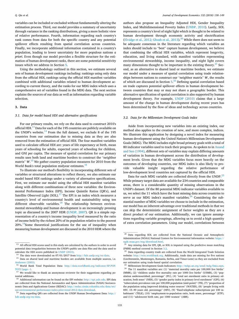
The rankings of official HDI fail to account for either uncertainty,spatial correlation, or population. Alternatively, we estimate our indexranks in terms of distributions, which provides a measure of uncertainty.Since factor weightings differ between our model based index and theofficial HDI, there must be some discordance between our posterior meanranks and the official HDI ranks. We graphically compare the two rank-ings, including information regarding the 99% confidence interval of theposterior ranks, in Fig. 1.

134

For Fig. 1 and subsequent figures of the same design, the dashed gridlines partition the 0%–20% (1st), 20%–40% (2nd), 40%–60% (3rd),60%–80% (4th), and 80%–100% (5th) quintiles of ranks, respectively.Solid dots show the locations of both posterior mean ranks and officialHDI ranks. The solid horizontal lines across each dot represent a 99%confidence interval for a country's posterior rank under our model. Thenumbers in Fig. 1 correspond to individual country identifiers, which areassigned alphabetically and listed in Appendix C.

Fig. 1 shows that our model's rankings harbor a considerable level ofuncertainty for certain countries, with several confidence intervalsreaching across multiple quintiles. Interestingly, this uncertainty persistsin various degrees along the entire distribution of ranks as opposed tobeing constrained to only certain levels of development. As an example,Bhutan, a low-development level country, has a posterior 99% confi-dence interval of (137, 164), implying that their rank could fall intoeither the 4th or the 5th quintile of human development. Comparableresults are also found for more highly developed nations like Qatar,which has a posterior 99% confidence interval of (15, 56), implying thatits rank could fall into either the 1st or 2nd quintile. While Bhutan andQatar represent more extreme cases, it is not uncommon for the confi-dence interval of certain nations to reach across quintiles of humandevelopment under our model.

The relationship between a country's rank and its level of uncertaintyis an inverted U-shape, with levels of uncertainty decreasing for the mostand least developed countries. This relationship is likely due to severalfactors. First, countries ranked at the top (bottom) have the highest(lowest) values for each manifest variable. Second, countries away fromthe distribution's center often tend to be the most highly populated,implying that they produce a lower degree of uncertainty in our model.Third, these countries are also closer to one another on averagegeographically, leading to a reduction in uncertainty through spatialsmoothing. This result with spatial correlation mirrors the geographicalclustering often observed in human development, i.e. having many low-development level countries in sub-Saharan Africa or many high-development level countries in Europe. Finally, the relationship be-tween development and uncertainty is also partially determined by thetruncation of variable values from either above or below for the most andleast developed countries.

Fig. 1 also illustrates the discordance between our model based ranksand those of the official HDI. The greater the distance between solid dotsand the 45o line, the greater the disagreement between our model basedranks and the ranks of official HDI. While the results of both models arewell correlated, for only eleven countries are the model based and officialHDI ranks identical. For 72 countries, the absolute value of the differencebetween both two ranks is less than five. For 53 countries, however, theabsolute value of the difference is larger than 10.

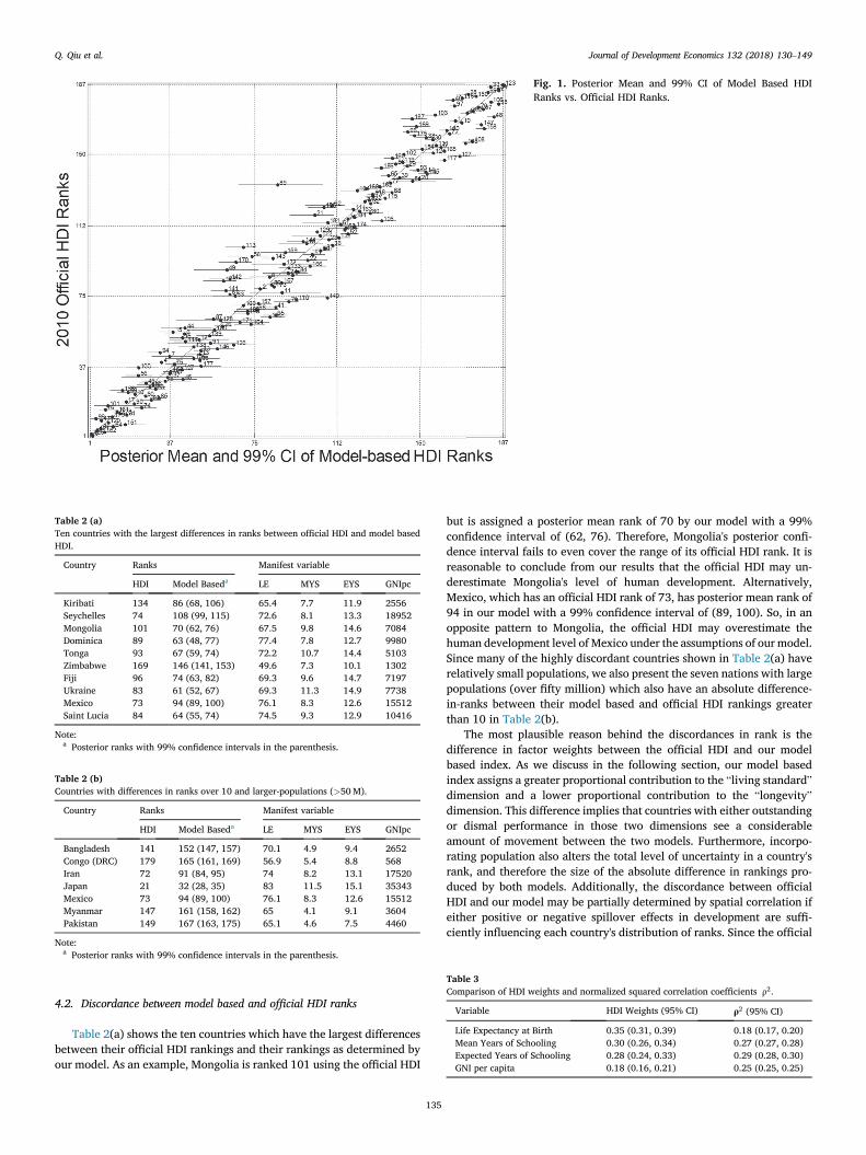
Fig. 1. Posterior Mean and 99% CI of Model Based HDIRanks vs. Official HDI Ranks.

Table 2 (a)Ten countries with the largest differences in ranks between official HDI and model basedHDI.

Country Ranks Manifest variable

HDI Model Baseda LE MYS EYS GNIpc

Kiribati 134 86 (68, 106) 65.4 7.7 11.9 2556Seychelles 74 108 (99, 115) 72.6 8.1 13.3 18952Mongolia 101 70 (62, 76) 67.5 9.8 14.6 7084Dominica 89 63 (48, 77) 77.4 7.8 12.7 9980Tonga 93 67 (59, 74) 72.2 10.7 14.4 5103Zimbabwe 169 146 (141, 153) 49.6 7.3 10.1 1302Fiji 96 74 (63, 82) 69.3 9.6 14.7 7197Ukraine 83 61 (52, 67) 69.3 11.3 14.9 7738Mexico 73 94 (89, 100) 76.1 8.3 12.6 15512Saint Lucia 84 64 (55, 74) 74.5 9.3 12.9 10416

Note:a Posterior ranks with 99% confidence intervals in the parenthesis.

Table 2 (b)Countries with differences in ranks over 10 and larger-populations (>50M).

Country Ranks Manifest variable

HDI Model Baseda LE MYS EYS GNIpc

Bangladesh 141 152 (147, 157) 70.1 4.9 9.4 2652Congo (DRC) 179 165 (161, 169) 56.9 5.4 8.8 568Iran 72 91 (84, 95) 74 8.2 13.1 17520Japan 21 32 (28, 35) 83 11.5 15.1 35343Mexico 73 94 (89, 100) 76.1 8.3 12.6 15512Myanmar 147 161 (158, 162) 65 4.1 9.1 3604Pakistan 149 167 (163, 175) 65.1 4.6 7.5 4460

Note:a Posterior ranks with 99% confidence intervals in the parenthesis.

Table 3Comparison of HDI weights and normalized squared correlation coefficients ρ2.

Variable HDI Weights (95% CI) ρ2 (95% CI)

Life Expectancy at Birth 0.35 (0.31, 0.39) 0.18 (0.17, 0.20)Mean Years of Schooling 0.30 (0.26, 0.34) 0.27 (0.27, 0.28)Expected Years of Schooling 0.28 (0.24, 0.33) 0.29 (0.28, 0.30)GNI per capita 0.18 (0.16, 0.21) 0.25 (0.25, 0.25)

Q. Qiu et al. Journal of Development Economics 132 (2018) 130–149

4.2. Discordance between model based and official HDI ranks

Table 2(a) shows the ten countries which have the largest differencesbetween their official HDI rankings and their rankings as determined byour model. As an example, Mongolia is ranked 101 using the official HDI

135

but is assigned a posterior mean rank of 70 by our model with a 99%confidence interval of (62, 76). Therefore, Mongolia's posterior confi-dence interval fails to even cover the range of its official HDI rank. It isreasonable to conclude from our results that the official HDI may un-derestimate Mongolia's level of human development. Alternatively,Mexico, which has an official HDI rank of 73, has posterior mean rank of94 in our model with a 99% confidence interval of (89, 100). So, in anopposite pattern to Mongolia, the official HDI may overestimate thehuman development level of Mexico under the assumptions of our model.Since many of the highly discordant countries shown in Table 2(a) haverelatively small populations, we also present the seven nations with largepopulations (over fifty million) which also have an absolute difference-in-ranks between their model based and official HDI rankings greaterthan 10 in Table 2(b).

The most plausible reason behind the discordances in rank is thedifference in factor weights between the official HDI and our modelbased index. As we discuss in the following section, our model basedindex assigns a greater proportional contribution to the “living standard”dimension and a lower proportional contribution to the “longevity”dimension. This difference implies that countries with either outstandingor dismal performance in those two dimensions see a considerableamount of movement between the two models. Furthermore, incorpo-rating population also alters the total level of uncertainty in a country'srank, and therefore the size of the absolute difference in rankings pro-duced by both models. Additionally, the discordance between officialHDI and our model may be partially determined by spatial correlation ifeither positive or negative spillover effects in development are suffi-ciently influencing each country's distribution of ranks. Since the official

Fig. 2. The Probability to be Model Based “Top 10” vs.Official HDI Ranks.

Q. Qiu et al. Journal of Development Economics 132 (2018) 130–149

HDI is a direct measurement built on observable variables, one couldinterpret our results under the assumption that the HDI is a “correct”measure. Assuming that the HDI is “correct”, we find that the posteriormean ranks of our model and the official HDI correlate well on average.Alternatively, we also evaluate the level of discordance between theofficial HDI and our model under the opposite assumption using simu-lated data where our model identifies the correct data generating processin Section 5.

4.3. Squared correlation coefficients

Due to differences in methodology, there is no simple way to comparethe estimated contributions of each manifest variable on the official HDI'smeasure of human development or the latent factor in our model. Tocalculate a general measure of comparability, we follow Ravallion (2012)who suggests calculating the marginal weights of each variable in theofficial HDI as the partial derivative of the official HDI with respect toeach observable variable. Following this approach, we obtain the mar-ginal weights of each variable in the official HDI by regressing stan-dardized HDI scores on standardized manifest variables.

To summarize each variable's contribution to the latent developmentfactor of our model, we apply the method of Hogan and Tchernis (2004)and present normalized “squared correlation coefficients.” The squaredcorrelation coefficient of each manifest variable j is specified as:

ρ2j ¼λ2j

λ2j þ σ2j

Each squared correlation coefficient corresponds to the proportion ofvariation in the manifest variable, j, that is explained by the latent humandevelopment factor. In Table 3, we compare the normalized marginalweights of each manifest variable from the official HDI to the normalizedsquared correlation coefficients produced by our model.

Concerning our results, we find that the “longevity” dimension offersa smaller contribution to human development than the weights of officialHDI would suggest. As Anand and Sen (1994) discuss, differences in theHDI ranks of high development level countries are largely driven byminor changes in relative life expectancy as their values for the otherinputs are largely similar. In turn, the increased importance of life ex-pectancy at the higher end of the distribution may inflate the relativeweight placed on the “longevity” dimension by official HDI. Our modelalso attributes a much greater contribution to the “living standard”

136

dimension when compared to official HDI. Additionally, while the offi-cial HDI assigns a greater proportional contribution to “mean years ofschooling” than “expected years of schooling,” our model estimates thatthe opposite is true. Therefore, under the assumptions of our model, theseresults suggest that the available data may not support the deterministicweights used to calculate official HDI. If this is indeed the case, the HDI'srankings may bias our understanding of relative human developmentlevels across countries, which in turn could impact both international andnational level policies targeting human development. On the other hand,we find that each of the official HDI's manifest variables providesconsiderable contributions to human development, indicating that thehuman development theory guiding the variable selection process issupported by both models.

4.4. The most and least developed countries

One of the HDI's primary purposes is identifying countries with boththe highest and lowest levels of human development. Distinguishingcountries with best practices establishes role models for other nationswhile identifying the least developed countries has significant economicand policy implications for nations with lower levels of human devel-opment. Since comparing relative performance is so important, it againbecomes a potential concern that the official HDI offers only a single rankfor each country as opposed to a plausible range of values. The lack ofuncertainty can be especially detrimental to countries falling just outsidethe lowest levels of human development, as it may disqualify them fromparticipating in beneficial international assistance programs if theirofficial HDI rank does not meet a program's requirements. Given that ourmethod produces distributions of ranks, we can estimate and assignprobabilities for each country to be within the most and least developedgroups.

In Fig. 2 we present the estimated likelihood of certain countriesbeing among the ten most developed countries using our model alongwith their official HDI rankings. Of the 187 countries, 17 have non-zeroprobabilities of being included in our model's “Top 10.” Of these 17countries, seven are not among the “Top 10” according to their officialHDI ranks, implying that they may be overlooked when evaluating thesuccessful actions of role model nations. In Fig. 3 we present the likeli-hood of certain countries being among the ten least developed countriesusing our model along with their official HDI rankings. Of the 13 coun-tries which have non-zero probabilities associated with being included in

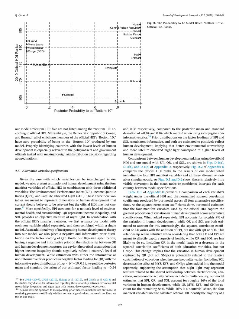
Fig. 3. The Probability to be Model Based “Bottom 10” vs.Official HDI Ranks.

Q. Qiu et al. Journal of Development Economics 132 (2018) 130–149

our model's “Bottom 10,” five are not listed among the “Bottom 10” ac-cording to official HDI. Mozambique, the Democratic Republic of Congo,and Burundi, all of which are members of the official HDI's “Bottom 10,”have zero probability of being in the “Bottom 10” produced by ourmodel. Properly identifying countries with the lowest levels of humandevelopment is especially relevant to the policymakers and governmentofficials tasked with making foreign aid distribution decisions regardingat-need nations.

4.5. Alternative variables specifications

Given the ease with which variables can be interchanged in ourmodel, we now present estimations of human development using the fourmanifest variables of official HDI in combination with three additionalvariables: The Environmental Performance Index (EPI), Income QuintileRatios (QR's), and Satellite Observed Light (SOL). These three new var-iables are meant to represent dimensions of human development thatcurrent theory believes to be relevant but the official HDI may not cap-ture.25 More specifically, EPI accounts for a nation's level of environ-mental health and sustainability, QR represents income inequality, andSOL provides an objective measure of night light. In combination withthe official HDI's manifest variables, we first estimate our model witheach new variable added separately, and then combined within a singlemodel. As an additional way of incorporating human development theoryinto our model, we also place a negative and informative prior distri-bution on the factor loading of QR. Under our Bayesian specification,having a negative and informative prior on the relationship between QRand human development captures the a priori theoretical assumption thathigher income inequality should negatively reflect a country's level ofhuman development. While estimation with either the informative ornon-informative prior produces a negative factor loading for QR, with theinformative prior distribution of λQR � Nð�10;0:1Þ, we pull the posteriormean and standard deviation of our estimated factor loading to �0.24

25 See UNDP (2007), UNDP (2010), Elvidge et al. (2012), and Ghosh et al. (2013) andthe studies they discuss for information regarding the relationship between environmentalstewardship, inequality, and night light with human development, respectively.26 A more extreme approach to incorporating prior theoretical beliefs into our model isrestricting parameters to fall only within a certain range of values, but we do not illustratethis in our study.

137

and 0.06 respectively, compared to the posterior mean and standarddeviation of �0.04 and 0.04 which we find when using a conjugate non-informative prior.26 Prior distributions on the factor loadings of EPI andSOL remain non-informative, and both are estimated to positively reflecthuman development, implying that better environmental stewardshipand more satellite observed night light correspond to higher levels ofhuman development.

Comparisons between human development rankings using the officialHDI and our model with EPI, QR, and SOL, are shown in Figs. D.1(a),D.1(b), and D.1(c) of Appendix D, respectively. Fig. D.2 of Appendix Dcompares the official HDI ranks to the results of our model whenincluding the four HDI manifest variables and all three alternative vari-ables simultaneously. As Figs. D.1 and D.2 show, there is relatively littlevisible movement in the mean ranks or confidence intervals for eachcountry between model specifications.

Table D.1 of Appendix D provides a comparison of each variable'sweight under the official HDI and the normalized squared correlationcoefficients produced by our model across all four alternative specifica-tions. As the squared correlation coefficients show, our model estimatesthat the four manifest variables used by the official HDI capture thegreatest proportion of variation in human development across alternativespecifications. When added separately, EPI accounts for roughly 9% ofthe variation in human development, while QR and SOL are both esti-mated to account for 4%. Interestingly, the squared correlation coeffi-cient on LE varies with the addition of EPI, but not with QR or SOL. Thisrelationship seems intuitive when considering that both LE and EPI aremeant to directly capture aspects of health, while QR and SOL are lesslikely to do so. Including QR in the model leads to a decrease in thesquared correlation coefficients of both education variables, but notGNIpc. This change implies that the variation in human developmentcaptured by QR (but not GNIpc) is potentially related to the relativecontribution of education when income inequality varies. Including SOLdecreases the effect of MYS, EYS, and GNIpc when added into the modelseparately, supporting the assumption that night light may representfeatures related to the shared relationship between electrification, edu-cation, and economic activity. When included simultaneously, our modelestimates that EPI, QR, and SOL account for roughly 16% of the totalvariation in human development, while LE, MYS, EYS, and GNIpc ac-count for the remaining 84%. While 16% is a nontrivial share, the fourmanifest variables used to calculate official HDI identify the majority of a

Fig. 4. Posterior Mean and 99% CI of Model Based MDGRanks using PMM.

Table 4MDG normalized squared correlation coefficients ρ2and signs of factor loadings λ usingPMM.

Variable ρ2  (95%CI)

With Naïve Imputation Sign of λ

TELE 0.15 (0.14, 0.16) þ

Q. Qiu et al. Journal of Development Economics 132 (2018) 130–149

country's human development level. Therefore, the issue regardinghuman development's measurement may be one of estimation methodmore so than variable selection. Comparing the level of discordancebetween the results of our base model and those of our model includingEPI, QR, and SOL shows that only one country (Kiribati) has an absolutedifference in rank greater than five.

TB 0.11 (0.10, 0.11) -U5MR 0.17 (0.16, 0.20) -WATER 0.11 (0.10, 0.11) þMMR 0.17 (0.15, 0.19) -PU 0.08 (0.08, 0.09) -GPI 0.03 (0.01, 0.04) þNER 0.06 (0.05, 0.07) þHIV 0.02 (0.01, 0.03) -ETP 0.00 (0.00, 0.01) þABR 0.10 (0.09, 0.10) -

4.6. Results for MDG index

We now present the results of our model estimated using manifestvariables from the Millennium Development Goals (MDG). Initially, weconstruct our MDG index using a naïve imputation process to estimateany missing data. We also estimate the index using posterior imputation,the results of which are discussed in Section 5. In Fig. 4, we compare theposterior mean ranks of our MDG index with the ranks of official HDIusing the naïvely imputed data. Fig. 4 shows a positive association be-tween the ranks of our “MDG index” and those of the official HDI whichwe would expect even between measures of human development usingdifferent variables.27

Because the MDG index includes both a greater number of variablesand variables which the official HDI does not use, it naturally produces ahigher level of discordance with the official HDI compared to our mainresults or those obtained from our alternative specifications built aroundthe four HDI manifest variables. More specifically, the sum of absolutedifferences between our model based HDI ranks and the ranks of officialHDI is 1,439, while the sum of absolute differences between the ranks ofour MDG index and the official HDI is 2448.28 Referencing the top-rightcorner of Fig. 4 for a visual example of the discordance between the twoindices, Equatorial Guinea, Congo, Zambia, Kenya, and Swaziland, noneof which fall into the lowest development quintile of official HDI, are alllocated in the lowest development quintile of our MDG index. Therefore,

27 The correlation between the posterior mean ranks of our MDG index and the ranks ofofficial HDI is roughly 0.95.28 The average absolute difference in ranks between the official HDI and MDG index is13.1.

138

the official HDI may overestimate the development levels of thesecountries under the assumptions of our MDG index. Given that the MDG'svariables focus more on developing countries, a driving factor of thisdiscordance may be information regarding the relative performance oflow development level countries across dimensions which are capturedby our MDG index but not by the HDI's manifest variables. Looking to thebottom-left corner of Fig. 4, Brunei, Qatar, and the United States are allranked outside of the most developed quintile of our posterior MDGranks while they are included in the most developed quintile of theofficial HDI. Therefore, it is possible that the official HDI overestimatesthe development level of these countries given our findings. We alsoestimate the total level of uncertainty in ranks produced by our MDGindex to be lower than our estimations using the HDI manifest variableswhich is most likely the result of including a greater number of totalvariables in the model.29

29 For example, the average standard deviation of ranks for our MDG index is 1.58compared to an average standard deviation of 2.25 for our model based HDI.

Q. Qiu et al. Journal of Development Economics 132 (2018) 130–149

Table 4 presents the normalized squared correlation coefficients forthe variables of our MDG index and the sign of their factor loadings. OurMDG index suggests that maternal mortality (MMR) and child mortality(U5MR) account for the greatest shares of variation in human develop-ment. The relative contributions of MMR and U5MR are both in line withthe assumption that an untimely death represents the worst-case humandevelopment scenario for individuals under a human outcomes focusedtheory of development. Alternatively, the adult HIV rate (HIV) andemployment-to-population ratio (ETP) account for the smallest amountsof variation in human development according to our MDG index.

5. Sensitivity analysis

In this section, we explore the sensitivity of our model's results acrossfour separate dimensions. First, we examine the change in our resultsusing an alternative specification of spatial correlation based on traderather than geographical boundaries. Second, we evaluate the roles ofordinality and cardinality in our model by estimating human develop-ment using the ranks, rather than raw values, of each country's observedoutcomes.30 Third, we evaluate the sensitivity of our model to imputationprocedure by comparing the results of our MDG index under both PMMand posterior imputation. Finally, we evaluate the performance of bothour model and the official HDI in a simulated data exercise where ourmodel is assumed to capture the correct data generating process.

5.1. Estimation with an alternative spatial correlation structure

Spatial correlation plays a significant role in our model as it allows forthe estimation of spillover effects in human development across coun-tries. We estimate the results presented in Section 4 under a framework ofspatial correlation where countries are considered “neighbors” if theyshare a common land or maritime border. This method of definingneighbors captures the geographic clustering of similar developmentlevel countries observed in the data (i.e. many low-development levelcountries in sub-Saharan Africa or many very-high development levelcountries in Europe). On the other hand, since the transfer of ideas andtechnologies related to human development is not restricted to countriessharing a common geographical border, a logical alternative is a spatialcorrelation framework based on trade flows between countries.

To evaluate the sensitivity of our model to changes in spatial corre-lation structure, we re-estimate our primary results using an alternative“neighbor matrix” W such that for two countries i and j,

Wij ¼ Wji ¼ ExportsijGDPiþGDPj

, where Exportsij is the sum of total exports shared

between both countries, and GDPi and GDPj are country i and j’s totalGDP, respectively. If i and j are not trading partners, Wij ¼ Wji ¼ 0.Finally, Wii ¼ 0. Fig. D.3 of Appendix D shows the correspondence be-tween the ranks of official HDI and the ranks of our model under thistrade-based framework of spatial correlation. As Fig. D.3 illustrates, theestimated ranks of our model using trade-based spatial correlationcorrelate well with those of official HDI. Comparing the results acrossmodels more closely, the average absolute deviation between the ranks ofofficial HDI and our trade-based model is 6.56.

Table D.2 of Appendix D compares the normalized squared correla-tion coefficients of our trade-based model with those of our primary re-sults. As the table shows, both specifications of spatial correlationproduce almost identical estimations of the covariance in human devel-opment explained by each manifest variable. Comparing both specifica-tions' posterior means and confidence intervals of the model's otherparameters shows that the only non-trivial difference comes from thespatial correlation parameter, ω, which has a mean posterior value of0.126 in our primary model and 4.25 in our trade-based specification. Of

30 We would again like to thank an anonymous reviewer for suggesting this test of ourmodel.

139

course, variation in ω between models is expected when altering theunderlying spatial correlation structure. Given these results, we concludethat our model is generally robust to spatial correlation specificationsregarding how countries are related with one another.

5.2. Estimation using ranks of manifest variables

Given that the outcome we are most interested in estimating is thehuman development ranks for each country, the roles of cardinality andordinality in our model are of particular importance. One dimension bywhich we can examine this is to compare the results of our model usingthe cardinal (raw) values of each manifest variable to the results we findusing ordinal (rank) values. By converting manifest variable values intoranks, each country's performance is evaluated only with regards to theirrelative standing rather than the magnitude to which their manifestvariable values differ. Naturally, the use of ranks preserves order, but italso limits the effect of outlier countries in variables like GNIpc whichharbor high degrees of variation.

Fig. D.4 of Appendix D presents the correspondence between theranks of official HDI and our primary model using rank values of eachmanifest variable. Compared to the results of our model using the rawmanifest variables shown in Fig. 1, the most obvious change between theraw and ranked models’ correspondences with official HDI is in the top-right-hand corner for the lowest development level countries. Comparingthe raw and rank manifest variable model rankings with official HDImore formally, however, we find the average absolute deviation in ranksto be almost identical, at 7.72 and 7.79, respectively.31 Alternatively,while the average levels of absolute discordance between models arenearly identical, some countries with outlier values for their manifestvariables see considerable changes in their posterior ranks. This resultimplies that using rankings of manifest variables may abstract away frompotentially valuable information coming from cardinal relationships inthe data. Table D.3 of Appendix D presents the normalized squaredcorrelation coefficients of our model when using raw manifest variablevalues and rank manifest variable values. Comparing the raw and rankmodels, Table D.3 shows that MYS and GNIpc see the most notablechange in their estimated contribution to human development. Giventhat the amount of discordance between both model specifications andthe official HDI change only trivially, however, we conclude that therankings of our model are generally robust to the ordinal transformationof manifest variables.

5.3. Results using posterior imputation

Following the naïve imputation method used to predict the missingMDG data, we next formulate our MDG index using the posterior impu-tation process built into our model. As spoken to in previous sections, asubstantial quantity of data is missing for the MDG index manifest vari-ables, implying that they must be imputed before estimation. For ourmain results, we use these imputed values as data without accounting forthe inherent uncertainty of the imputation process. As an alternative, wenow incorporate the imputation of missing data into the estimation al-gorithm. Unlike our naïve imputation method, posterior imputationdraws from a posterior distribution of missing values during each itera-tion of the sampler. We present the results of our MDG index underposterior imputation graphically in Fig. D.5 of Appendix D.

While the posterior mean rank for most countries remains stable, theuncertainty of rankings following posterior imputation appears muchlarger for some countries when compared to the uncertainty of the naïveimputation results. More specifically, the more missing data a countryhas, the more uncertainty it will show following posterior imputation.This relationship leads countries like Liechtenstein and Hong Kong to

31 The standard deviation for the absolute deviations of both models are also nearlyidentical, at 7.04 for the raw model and 7.11 for the rank model.

Q. Qiu et al. Journal of Development Economics 132 (2018) 130–149

have extreme confidence intervals compared to the average. Addition-ally, higher levels of missing data increase the magnitude of separationbetween a country's naïve and posterior imputation mean ranks.

Formally measuring the amount of discordance between our modelunder the two imputation processes with the official HDI, we see an in-crease in the sum of squared differences in rank from 51,410 to 64,890using posterior imputation, a change of roughly 26%. While the sum ofsquared differences increases considerably following posterior imputa-tion, the sum of absolute differences remains relatively unchanged (a 3%increase from 2444 to 2522).32 This result implies that several outliercountries see a considerable change in rank between the two imputationmethods while the general discordance changes a comparably smallamount for countries with less missing data.

Table D.4 of Appendix D shows the normalized squared correlationcoefficients of our MDG index under both naïve and posterior imputa-tion. Our model still estimates that MMR and U5MR account for thegreatest proportion of covariance in human development, while NER,HIV, and ABR see the most significant amount of relative change betweenboth models. Since posterior imputation extrapolates the non-missingrelationship between a manifest variable and the latent factor onto themissing data, changes in the magnitude of each squared correlation co-efficient reflect the observed effect's strength. For example, the increasedeffect of HIV under posterior imputation suggests that HIV is highlyreflective of human development in the non-missing portion of our data.Using non-Bayesian methods to estimate an MDG index would forcepractitioners to rely on naïve imputation and potentially miss theprominent level of contribution variables like HIV expresses in the non-missing data.

5.4. Simulated data exercise

Since both our model and the official HDI are inherently incompletemodels of human development, it is important that we better understandthe relative capabilities of each approach. One way to evaluate the per-formance of both models is using a simulation where we can directlyspecify the true underlying relationship of the data. More specifically, weuse the posterior mean parameter values estimated with our model underreal data to simulate a set of data for each of the official HDI's fourmanifest variables using the assumed data generating process of ourmodel. The outcome of our simulation is a set of artificial data for all 187countries which we know matches the assumptions of our model.

Comparing the results of official HDI to our model using simulateddata shows that the level of average absolute deviation between ranksincreases by nearly a factor of three.33 Furthermore, our model can es-timate each data generating parameter to within one standard deviationof the posterior mean. We present the data generating parameter valuesand the estimated posterior means and standard deviations in Table D.5of Appendix D. Given that the official HDI is a direct measure as opposedto a model which assumes an underlying data generating process, one caninterpret our results using real data under the assumption that the officialHDI is the “correct” measure of human development. Under thisassumption, the results discussed in Section 4 show that the posteriormean ranks of our model are well correlated with the ranks of officialHDI. Under the opposite assumption that our model is correct, thesimulated data exercise shows that the official HDI is not able to achieve asimilar level of agreement using data for which we know our modelidentifies the true data generating process. This result suggests that ourmodel is more flexible when estimating human development using datagenerated from different sources relative to the official HDI.

32 The average of absolute differences in rank increases from 13.07 to 13.49, and thestandard deviation of absolute differences between ranks increases from 10.2 to 12.9.33 The average absolute deviation in ranks between the official HDI and our model goesfrom 7.7 using real data to 22.0 using simulated data.

140

6. Conclusion

In this paper, we propose a Bayesian factor analysis model whichserves as both an alternative approach to calculating the UNDP's HumanDevelopment Index and a general methodology which can be used toeither augment existing indices or build new ones. We address severaltechnical issues of the official HDI in the following ways. First, our modelproduces data-driven weights for each manifest variable's contribution tothe latent factor of human development. Informing weights withobserved data stands in contrast to the ad hoc factor weights used tocalculate the ranks of official HDI. Second, our model estimates its ranksin terms of distributions, allowing for a measure of uncertainty which isabsent from the official HDI. This measure of uncertainty provides a moreholistic view of relative performance across countries. Finally, we adjustthe uncertainty in ranks by incorporating a measure of spatial correlationbetween countries while also including country populations in our esti-mation. These additions improve the precision of our rank distributionsand allow for the estimation of spillover effects in human development.

Using our model to estimate human development with the sameobserved variables as the official HDI, we find that the “living standard”dimension provides a greater proportional contribution to humandevelopment than it is assigned by the official HDI, while the “longevity”dimension provides a lower proportional contribution. The results of ourmodel also show considerable levels of disagreement when compared tothe ranks of the official HDI. Under our model, it is is not uncommon forthe confidence intervals of country ranks to cover more than one quintileof human development level. Therefore, a country's relative performanceaccording to the rankings of our model may vary considerably whencompared to its relative performance according to the official HDI.

Aside from its technical advantages, we show the flexibility of ourmethodology by estimating human development with three additionalvariables not used in the official HDI and by creating a novel MDG indexusing data from the Millennium Development Goals. As our alternativespecifications illustrate, sets of variables can easily be added or removedfrom our model without fundamentally restructuring its estimation. Thisstands in contrast to the HDI's rigidity with respect to variable selectionwhich makes the addition or removal of information impractical. We findthat EPI, QR, and SOL explain roughly 16% of the total variation inhuman development when estimated along with the official HDI manifestvariables. Under the assumptions of our model, this result implies thatthe alternative variables account for variation across dimensions ofhuman development not captured by the official HDI. Therefore, ourmodel supports the use of alternative human development indices such asthe Inequality Adjusted HDI, Gender Inequality Index, and Multidimen-sional Poverty Index proposed by the 2010 HDR (UNDP, 2010). Asopposed to the official HDI and its related indices, however, our modelprovides a convenient framework for measuring an index using differentmanifest variables. Additionally, even with the complicated structure ofthe MDG's indicator variables, we show that our approach is suited toconstructing the desired index. The MDG index not only exemplifies theadaptive nature of our methodology, but also provides a blueprint whichresearchers can follow to build indices that may have previously seemedtoo complex. The results of our MDG index suggest that mother and childmortality outcomes explain the greatest proportions of covariance inhuman development. This finding is supported by the assumption thatearly death represents one of the most severe and adverse outcomes forcountries under the human-centered theory of development that mea-sures like the HDI are meant to represent. Future studies of humandevelopment may wish to examine the effect of these mortality measuresby incorporating them directly in models of development as opposed torelying on the official HDI's life expectancy measure.

We also evaluate the sensitivity of our model across several di-mensions. First, we estimate human development ranks using an alter-native specification of spatial correlation built on trade rather thangeographical borders. On average, we find that our estimates remainstable across specifications, implying that our model is robust to different

Q. Qiu et al. Journal of Development Economics 132 (2018) 130–149

definitions of spatial correlation. Second, to evaluate the role of cardi-nality and ordinality in our model, we estimate human developmentusing the rankings of each manifest variable as opposed to their rawvalues. The squared correlation coefficients of our model change acrossspecifications, but the average absolute deviation in ranks between theofficial HDI and our model remains nearly constant. Alternatively, someoutlier countries see relatively significant changes in their rank using therank model, implying that we may be losing information captured bydifferences in magnitude when not using raw variable values. Third, toaccount for the inherent uncertainty of imputation in our estimation ofthe MDG index, we compare the results of our model using both naïveand posterior imputation. We find that posterior imputation leads to anincrease in the discordance between our ranks and the ranks of officialHDI for some countries with substantial amounts of missing data, butminimal movement in the discordance on average. Finally, since both theofficial HDI and our model are incomplete measures of human devel-opment, we perform a simulated data exercise where our model assumes

141

the correct data generating process. In our simulated exercise, theaverage absolute difference between the ranks produced by the officialHDI and our model increase by nearly a factor of three compared to re-sults when using real data. This result implies that while the rankings ofour model are very close on average to those of the official HDI under theassumption that the HDI is “correct” when using real data, the officialHDI is not able to do the same in a simulation where the assumption isreversed.

Acknowledgements

We would like to thank Spencer Banzhaf, Alberto Chong, AndrewFoster, Christopher Udry, an anonymous reviewer, and the participantsof The 2nd International Workshop in Memory of Yair Mundlak for theirvaluable comments and suggestions. This research did not receive anyspecific grant from funding agencies in the public, commercial, or not-for-profit sectors.

Appendix A. Supplementary data

Supplementary data related to this article can be found at https://doi.org/10.1016/j.jdeveco.2017.12.007.

Appendix B. Gibbs sampler algorithm

Following Hogan and Tchernis (2004), our hierarchical factor analysis model is as follows:

Y��δ � N

�μþ Λδ;M�1 � Σ

�

δ � N�0;M�1

2ψM�12

�

where:

μ ¼ ½μ1; μ2; μ3; μ4�0;Λ ¼ IN � λ, with λ ¼ ½λ1; λ2; λ3; λ4�0;ψ ¼ ðI � ωWÞ�1;Σ ¼ diagðσ21; σ22; σ23; σ24Þ with all the off-diagonal elements equal to 0.

Therefore, the parameters to estimate are λ δ, μ, Σ and ω.Step 1: Sample elements of. λ:Let 1N be an N � 1 vector with all elements equal to 1. Therefore, for each λj; j ¼ 1;2;3; 4, let the estimation equation be Yj � 1N 'μj ¼ λjδþ εj, where

Yj is the N � 1 vector of manifest variable Yij, and εj � Nð0; σ2j =MÞ. Let the prior distribution be λj � Nða;AÞ, where a ¼ 0; A ¼ 1000. Hence, theposterior of Λjis drawn from conditional distribution Nðb; BÞ, where:

B ¼�1=Aþ δ0Mδ

.σ2j��1

b ¼ Bha=Aþ δ0M

�Yj � 1Nμj

�.σ2ji

As factor loadings, λj’s, are restricted to be positive.Step 2: Sample δ.Let the estimation equation be Y � μ� 1N ¼ Λδþ ε, where Y is the NJ � 1 vector of manifest variable Yij, and ε � Nð0;M�1 � ΣÞ. Given that the

prior distribution is δ � N�0;M�1

2ψM�12

�.

Hence, the posterior of δ is drawn from conditional distribution Nðd;DÞ, where:

D ¼��

M�12ψM�1

2

��1þ Λ0�M�1 � Σ

��1Λ

�1

d ¼ DhΛ0�M�1 � Σ

��1ðY � μ� 1NÞi

Step 3: Sample elements of μ.For each μj; j ¼ 1; 2; 3;4, let the estimation equation be Yj � λjδ ¼ 1Nμj þ εj. Let the prior distribution be μj � Nðc;CÞ, where c ¼ 0; C ¼ 1000.Hence, the posterior of μj is drawn from conditional distribution Nðe; EÞ, where:

Q. Qiu et al. Journal of Development Economics 132 (2018) 130–149

E ¼�1=C þ 1N 0M1N

.σ2j��1

e ¼ Ehc=C þ 10NM

�Yj � λjδ

�.σ2ji

Step 4: Sample elements of Σ.For each σ2j ; j ¼ 1;2; 3; 4, let the estimation equation be Yj ¼ λjδþ 1Nμj þ εj. Let the prior distribution be σ2j � IGðα0; β0Þ, where

α0 ¼ 0:001; β0 ¼ 0:001.Hence, the posterior of σ2j is drawn from conditional distribution IGðα1; β1Þ, where:

α1 ¼ α0 þ N2

β1 ¼�Yj � λjδ� 1Nμj

�0M�Yj � λjδ� 1Nμj

�þ β0

Step 5: Sample ω using a Metropolis-Hasting algorithm.Let the prior distribution of ω be πðωÞ ¼ Nð0; 1000ÞIðξ�1

1 < ω < ξ�1N Þ, where ξ1 and ξN denote the minimum andmaximum eigenvalues of the spatial

correlation matrix W . Hence, the target density of ω is f ðδjψðωÞÞπðωÞ, where f ðδjψðωÞÞ is the kernel of the distribution of δ conditional onψ ¼ ðI � ωWÞ�1. Let the proposal density be qðω'jωÞ � Nðω; ρ2Þ, so that the candidate ω' is drawn from a random walk equation: ω' ¼ ωþ ε, where ε �Nð0; ρ2Þ , and ρ2 is a tuning parameter. The generated ω is also restricted to the domain ξ�1

1 < ω < ξ�1N .

Therefore, ω' is accepted with probability:

min1;f ðδjψðω0ÞÞπðω0Þqðωjω0Þf ðδjψðωÞÞπðωÞqðω0jωÞ

�

Appendix C. Numbering of countries

# Country

1

Afghanistan 2 Albania 3 Algeria 4 Andorra 5 Angola 6 Antigua and Barbuda 7 Argentina 8 Armenia 9 Australia 10 Austria 11 Azerbaijan 12 Bahamas 13 Bahrain 14 Bangladesh 15 Barbados 16 Belarus 17 Belgium 18 Belize 19 Benin 20 Bhutan 21 Bolivia (Plurinational State of) 22 Bosnia and Herzegovina 23 Botswana 24 Brazil 25 Brunei Darussalam 26 Bulgaria 27 Burkina Faso 28 Burundi 29 Cambodia 30 Cameroon 31 Canada 32 Cape Verde 33 Central African Republic 34 Chad 35 Chile 36 China 37 Colombia 38 Comoros 39 Congo 40 Congo (Democratic Republic of the) 41 Costa Rica 42 Croatia 43 Cuba

(continued on next page)

142

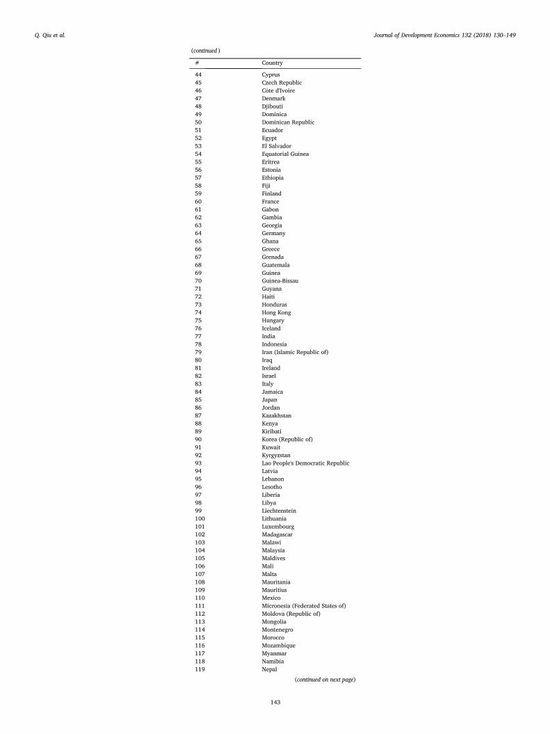
Q. Qiu et al. Journal of Development Economics 132 (2018) 130–149

(continued )

#

Country

44

Cyprus 45 Czech Republic 46 Cote d'Ivoire 47 Denmark 48 Djibouti 49 Dominica 50 Dominican Republic 51 Ecuador 52 Egypt 53 El Salvador 54 Equatorial Guinea 55 Eritrea 56 Estonia 57 Ethiopia 58 Fiji 59 Finland 60 France 61 Gabon 62 Gambia 63 Georgia 64 Germany 65 Ghana 66 Greece 67 Grenada 68 Guatemala 69 Guinea 70 Guinea-Bissau 71 Guyana 72 Haiti 73 Honduras 74 Hong Kong 75 Hungary 76 Iceland 77 India 78 Indonesia 79 Iran (Islamic Republic of) 80 Iraq 81 Ireland 82 Israel 83 Italy 84 Jamaica 85 Japan 86 Jordan 87 Kazakhstan 88 Kenya 89 Kiribati 90 Korea (Republic of) 91 Kuwait 92 Kyrgyzstan 93 Lao People's Democratic Republic 94 Latvia 95 Lebanon 96 Lesotho 97 Liberia 98 Libya 99 Liechtenstein 100 Lithuania 101 Luxembourg 102 Madagascar 103 Malawi 104 Malaysia 105 Maldives 106 Mali 107 Malta 108 Mauritania 109 Mauritius 110 Mexico 111 Micronesia (Federated States of) 112 Moldova (Republic of) 113 Mongolia 114 Montenegro 115 Morocco 116 Mozambique 117 Myanmar 118 Namibia 119 Nepal

(continued on next page)

143

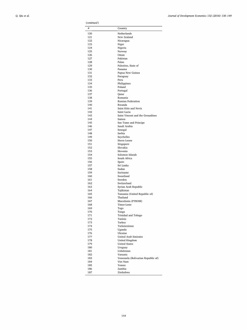
Q. Qiu et al. Journal of Development Economics 132 (2018) 130–149

(continued )

#

Country

120

Netherlands 121 New Zealand 122 Nicaragua 123 Niger 124 Nigeria 125 Norway 126 Oman 127 Pakistan 128 Palau 129 Palestine, State of 130 Panama 131 Papua New Guinea 132 Paraguay 133 Peru 134 Philippines 135 Poland 136 Portugal 137 Qatar 138 Romania 139 Russian Federation 140 Rwanda 141 Saint Kitts and Nevis 142 Saint Lucia 143 Saint Vincent and the Grenadines 144 Samoa 145 Sao Tome and Principe 146 Saudi Arabia 147 Senegal 148 Serbia 149 Seychelles 150 Sierra Leone 151 Singapore 152 Slovakia 153 Slovenia 154 Solomon Islands 155 South Africa 156 Spain 157 Sri Lanka 158 Sudan 159 Suriname 160 Swaziland 161 Sweden 162 Switzerland 163 Syrian Arab Republic 164 Tajikistan 165 Tanzania (United Republic of) 166 Thailand 167 Macedonia (FYROM) 168 Timor-Leste 169 Togo 170 Tonga 171 Trinidad and Tobago 172 Tunisia 173 Turkey 174 Turkmenistan 175 Uganda 176 Ukraine 177 United Arab Emirates 178 United Kingdom 179 United States 180 Uruguay 181 Uzbekistan 182 Vanuatu 183 Venezuela (Bolivarian Republic of) 184 Viet Nam 185 Yemen 186 Zambia 187 Zimbabwe

144

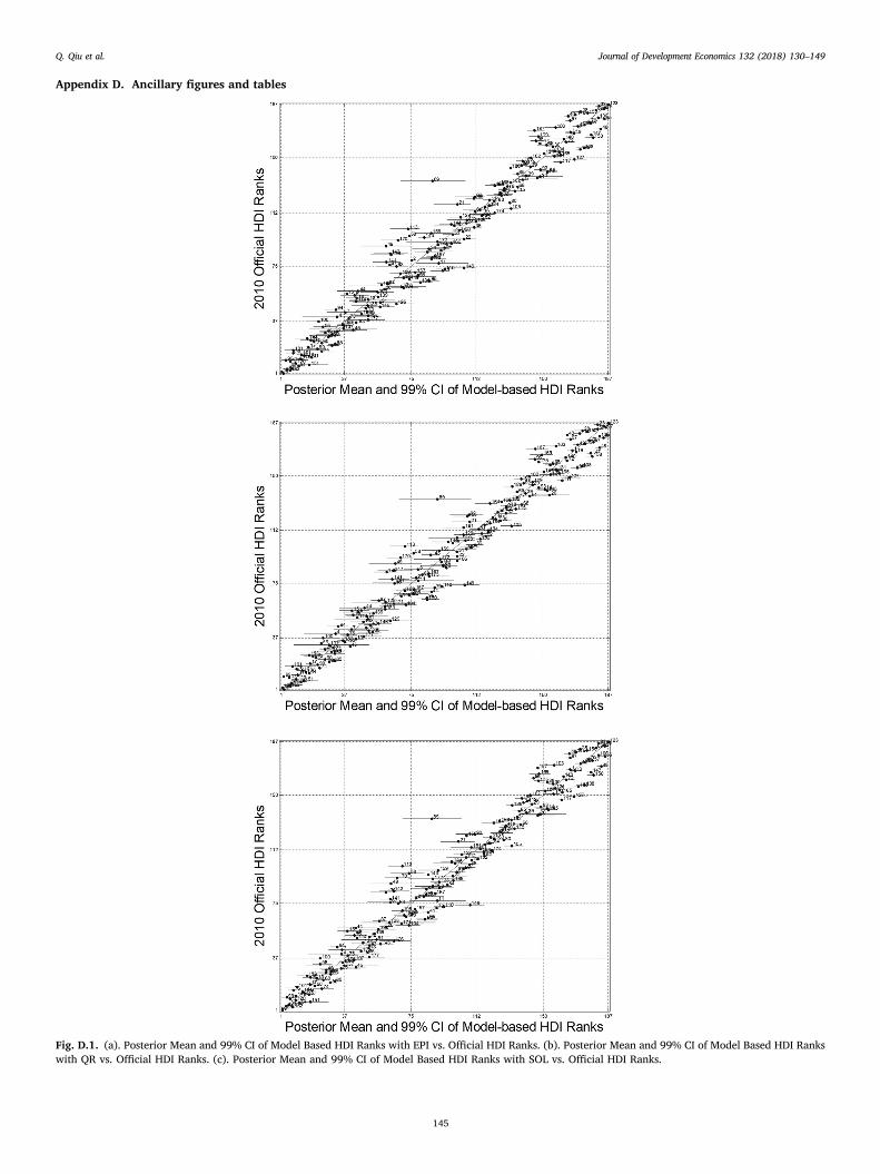
Q. Qiu et al. Journal of Development Economics 132 (2018) 130–149

Appendix D. Ancillary figures and tables

Fig. D.1. (a). Posterior Mean and 99% CI of Model Based HDI Ranks with EPI vs. Official HDI Ranks. (b). Posterior Mean and 99% CI of Model Based HDI Rankswith QR vs. Official HDI Ranks. (c). Posterior Mean and 99% CI of Model Based HDI Ranks with SOL vs. Official HDI Ranks.

145

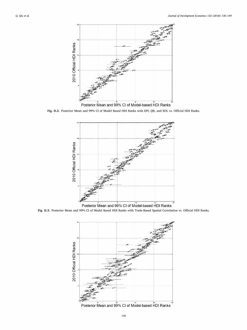
Journal of Development Economics 132 (2018) 130–149

Q. Qiu et al.

Fig. D.2. Posterior Mean and 99% CI of Model Based HDI Ranks with EPI, QR, and SOL vs. Official HDI Ranks.

Fig. D.3. Posterior Mean and 99% CI of Model Based HDI Ranks with Trade-Based Spatial Correlation vs. Official HDI Ranks.

146

Journal of Development Economics 132 (2018) 130–149

Fig. D.4. Posterior Mean and 99% CI of Model Based HDI Ranks with Ranked Manifest Variables vs. Official HDI Ranks.

Q. Qiu et al.

Fig. D.5. Posterior Mean and 99% CI of Model Based MDG Ranks Using Posterior Imputation vs. Official HDI Ranks.

Table D.1Comparison of HDI Weights and Normalized Squared Correlations ρ2 Adding Other Manifest Variables.

Variable HDI Weights (95% CI) ρ2(95% CI)

Base Model

147

Added Separately

Added Together

LE

0.35 (0.31, 0.39) 0.18 (0.17, 0.20) 0.17 (0.15,0.18) 0.18 (0.17,0.19) 0.18 (0.16,0.19) 0.16 (0.15,0.16) MYS 0.30 (0.26, 0.34) 0.27 (0.27, 0.28) 0.25 (0.24,0.25) 0.26 (0.25,0.27) 0.26 (0.25,0.27) 0.22 (0.21,0.25) EYS 0.28 (0.24, 0.33) 0.29 (0.28, 0.30) 0.26 (0.25,0.28) 0.27 (0.25,0.29) 0.28 (0.26,0.30) 0.24 (0.21,0.26) GNIpc 0.18 (0.16, 0.21) 0.25 (0.25, 0.25) 0.23 (0.23,0.24) 0.25 (0.24,0.25) 0.24 (0.24,0.25) 0.22 (0.20,0.23) EPI 0.09 (0.07,0.11) 0.09 (0.07,0.11) QR 0.04 (0.02,0.07) 0.04 (0.02,0.06) SOL 0.04 (0.02,0.06) 0.04 (0.02,0.06)

Table D.2Normalized Squared Correlations ρ2 of Model Based HDI Ranks with Trade-based SpatialCorrelation vs. Model Based HDI Ranks with Geographically-Based Spatial Correlation.

Variable ρ2  (95%CI)

Geographically-Based

Trade-Based

LE

0.18 (0.17, 0.20) 0.18 (0.16, 0.20) MYS 0.27 (0.27, 0.28) 0.27 (0.27, 0.28) EYS 0.29 (0.28, 0.30) 0.29 (0.28, 0.30) GNIpc 0.25 (0.25, 0.25) 0.26 (0.26, 0.26)

Table D.3Normalized Squared Correlations ρ2of Model Based HDI Ranks Using Raw ManifestVariable Values vs. Model Based HDI Ranks Using Ranked Manifest Variable Values.

Variable ρ2  (95%CI)

Raw Values

Ranked Values

LE

0.18 (0.17, 0.20) 0.17 (0.15, 0.18) MYS 0.27 (0.27, 0.28) 0.23 (0.23, 0.23) EYS 0.29 (0.28, 0.30) 0.31 (0.31, 0.33) GNIpc 0.25 (0.25, 0.25) 0.29 (0.28, 0.29)

Table D.4MDG Normalized Squared Correlation ρ2and Signs of Factor Loadings λ Using PMM vs. Posterior Imputation.

Variable ρ2(95%CI) Sign of λ

With PMM Imputation

With Posterior Imputation

TELE

0.15 (0.14, 0.16) 0.17 (0.15, 0.19) þ TB 0.11 (0.10, 0.11) 0.12 (0.11, 0.12) -

(continued on next page)

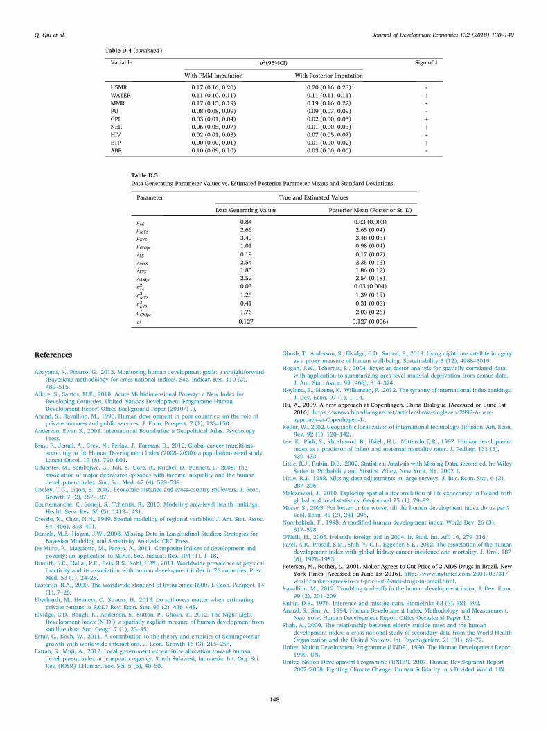
Q. Qiu et al. Journal of Development Economics 132 (2018) 130–149

Table D.4 (continued )

Variable

ρ2(95%CI)

148

Sign of λ

With PMM Imputation

With Posterior Imputation

U5MR

0.17 (0.16, 0.20) 0.20 (0.16, 0.23) - WATER 0.11 (0.10, 0.11) 0.11 (0.11, 0.11) þ MMR 0.17 (0.15, 0.19) 0.19 (0.16, 0.22) - PU 0.08 (0.08, 0.09) 0.09 (0.07, 0.09) - GPI 0.03 (0.01, 0.04) 0.02 (0.00, 0.03) þ NER 0.06 (0.05, 0.07) 0.01 (0.00, 0.03) þ HIV 0.02 (0.01, 0.03) 0.07 (0.05, 0.07) - ETP 0.00 (0.00, 0.01) 0.01 (0.00, 0.02) þ ABR 0.10 (0.09, 0.10) 0.03 (0.00, 0.06) -

Table D.5Data Generating Parameter Values vs. Estimated Posterior Parameter Means and Standard Deviations.

Parameter True and Estimated Values

Data Generating Values

Posterior Mean (Posterior St. D)

μLE

0.84 0.83 (0.003) μMYS 2.66 2.65 (0.04) μEYS 3.49 3.48 (0.03) μGNIpc 1.01 0.98 (0.04) λLE 0.19 0.17 (0.02) λMYS 2.54 2.35 (0.16) λEYS 1.85 1.86 (0.12) λGNIpc 2.52 2.54 (0.18) σ2LE 0.03 0.03 (0.004)

σ2MYS

1.26 1.39 (0.19)

σ2EYS

0.41 0.31 (0.08)

σ2GNIpc

1.76 2.03 (0.26)

ω

0.127 0.127 (0.006)

References

Abayomi, K., Pizarro, G., 2013. Monitoring human development goals: a straightforward(Bayesian) methodology for cross-national indices. Soc. Indicat. Res. 110 (2),489–515.

Alkire, S., Santos, M.E., 2010. Acute Multidimensional Poverty: a New Index forDeveloping Countries. United Nations Development Programme HumanDevelopment Report Office Background Paper (2010/11).

Anand, S., Ravallion, M., 1993. Human development in poor countries: on the role ofprivate incomes and public services. J. Econ. Perspect. 7 (1), 133–150.

Anderson, Ewan S., 2003. International Boundaries: a Geopolitical Atlas. PsychologyPress.

Bray, F., Jemal, A., Grey, N., Ferlay, J., Forman, D., 2012. Global cancer transitionsaccording to the Human Development Index (2008–2030): a population-based study.Lancet Oncol. 13 (8), 790–801.

Cifuentes, M., Sembajwe, G., Tak, S., Gore, R., Kriebel, D., Punnett, L., 2008. Theassociation of major depressive episodes with income inequality and the humandevelopment index. Soc. Sci. Med. 67 (4), 529–539.

Conley, T.G., Ligon, E., 2002. Economic distance and cross-country spillovers. J. Econ.Growth 7 (2), 157–187.

Courtemanche, C., Soneji, S., Tchernis, R., 2015. Modeling area-level health rankings.Health Serv. Res. 50 (5), 1413–1431.

Cressie, N., Chan, N.H., 1989. Spatial modeling of regional variables. J. Am. Stat. Assoc.84 (406), 393–401.

Daniels, M.J., Hogan, J.W., 2008. Missing Data in Longitudinal Studies: Strategies forBayesian Modeling and Sensitivity Analysis. CRC Press.

De Muro, P., Mazziotta, M., Pareto, A., 2011. Composite indices of development andpoverty: an application to MDGs. Soc. Indicat. Res. 104 (1), 1–18.

Dumith, S.C., Hallal, P.C., Reis, R.S., Kohl, H.W., 2011. Worldwide prevalence of physicalinactivity and its association with human development index in 76 countries. Prev.Med. 53 (1), 24–28.

Easterlin, R.A., 2000. The worldwide standard of living since 1800. J. Econ. Perspect. 14(1), 7–26.

Eberhardt, M., Helmers, C., Strauss, H., 2013. Do spillovers matter when estimatingprivate returns to R&D? Rev. Econ. Stat. 95 (2), 436–448.

Elvidge, C.D., Baugh, K., Anderson, S., Sutton, P., Ghosh, T., 2012. The Night LightDevelopment Index (NLDI): a spatially explicit measure of human development fromsatellite data. Soc. Geogr. 7 (1), 23–35.

Ertur, C., Koch, W., 2011. A contribution to the theory and empirics of Schumpeteriangrowth with worldwide interactions. J. Econ. Growth 16 (3), 215–255.

Fattah, S., Muji, A., 2012. Local government expenditure allocation toward humandevelopment index at jeneponto regency, South Sulawesi, Indonesia. Int. Org. Sci.Res. (IOSR) J.Human. Soc. Sci. 5 (6), 40–50.

Ghosh, T., Anderson, S., Elvidge, C.D., Sutton, P., 2013. Using nighttime satellite imageryas a proxy measure of human well-being. Sustainability 5 (12), 4988–5019.

Hogan, J.W., Tchernis, R., 2004. Bayesian factor analysis for spatially correlated data,with application to summarizing area-level material deprivation from census data.J. Am. Stat. Assoc. 99 (466), 314–324.

Høyland, B., Moene, K., Willumsen, F., 2012. The tyranny of international index rankings.J. Dev. Econ. 97 (1), 1–14.

Hu, A., 2009. A new approach at Copenhagen. China Dialogue [Accessed on June 1st2016]. https://www.chinadialogue.net/article/show/single/en/2892-A-new-approach-at-Copenhagen-1-.

Keller, W., 2002. Geographic localization of international technology diffusion. Am. Econ.Rev. 92 (1), 120–142.

Lee, K., Park, S., Khoshnood, B., Hsieh, H.L., Mittendorf, R., 1997. Human developmentindex as a predictor of infant and maternal mortality rates. J. Pediatr. 131 (3),430–433.

Little, R.J., Rubin, D.B., 2002. Statistical Analysis with Missing Data, second ed. In: WileySeries in Probability and Stistics. Wiley, New York, NY. 2002 1.

Little, R.J., 1988. Missing-data adjustments in large surveys. J. Bus. Econ. Stat. 6 (3),287–296.

Malczewski, J., 2010. Exploring spatial autocorrelation of life expectancy in Poland withglobal and local statistics. Geojournal 75 (1), 79–92.

Morse, S., 2003. For better or for worse, till the human development index do us part?Ecol. Econ. 45 (2), 281–296.

Noorbakhsh, F., 1998. A modified human development index. World Dev. 26 (3),517–528.

O'Neill, H., 2005. Ireland's foreign aid in 2004. Ir. Stud. Int. Aff. 16, 279–316.Patel, A.R., Prasad, S.M., Shih, Y.-C.T., Eggener, S.E., 2012. The association of the human

development index with global kidney cancer incidence and mortality. J. Urol. 187(6), 1978–1983.

Petersen, M., Rother, L., 2001. Maker Agrees to Cut Price of 2 AIDS Drugs in Brazil. NewYork Times [Accessed on June 1st 2016]. http://www.nytimes.com/2001/03/31/world/maker-agrees-to-cut-price-of-2-aids-drugs-in-brazil.html.

Ravallion, M., 2012. Troubling tradeoffs in the human development index. J. Dev. Econ.99 (2), 201–209.

Rubin, D.B., 1976. Inference and missing data. Biometrika 63 (3), 581–592.Anand, S., Sen, A., 1994. Human Development Index: Methodology and Measurement.

New York: Human Development Report Office Occasional Paper 12.Shah, A., 2009. The relationship between elderly suicide rates and the human

development index: a cross-national study of secondary data from the World HealthOrganization and the United Nations. Int. Psychogeriatr. 21 (01), 69–77.

United Nation Development Programme (UNDP), 1990. The Human Development Report1990. UN.

United Nation Development Programme (UNDP), 2007. Human Development Report2007/2008: Fighting Climate Change: Human Solidarity in a Divided World. UN.

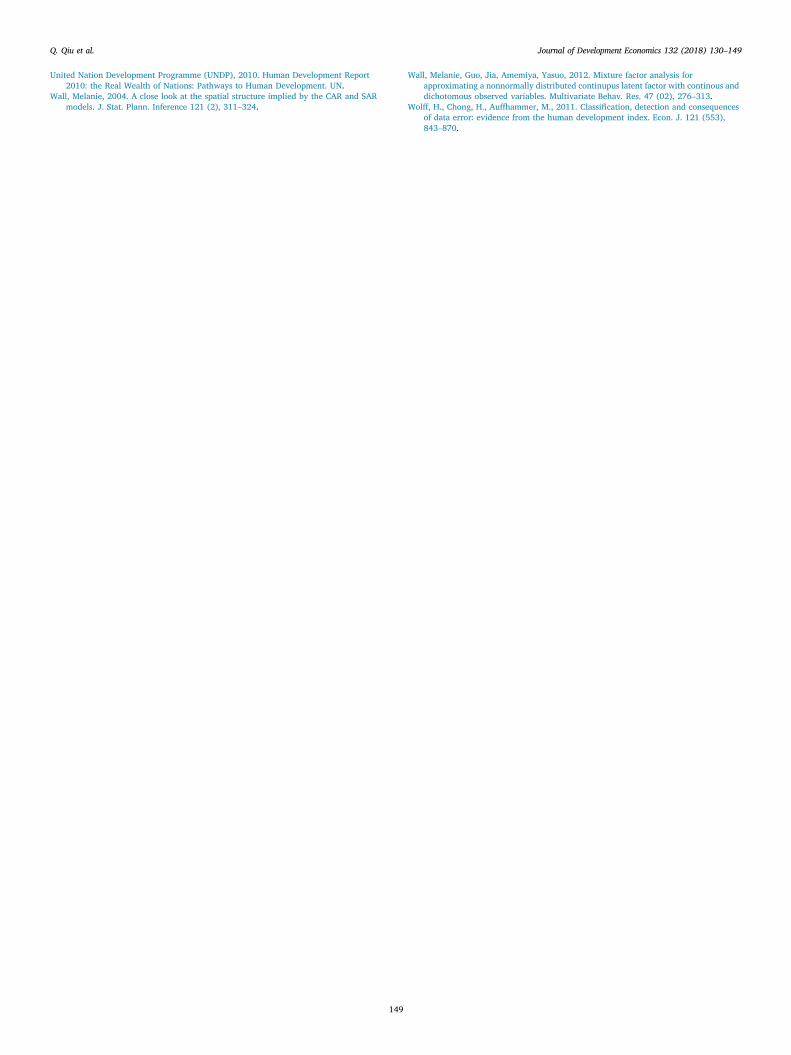
Q. Qiu et al. Journal of Development Economics 132 (2018) 130–149

United Nation Development Programme (UNDP), 2010. Human Development Report2010: the Real Wealth of Nations: Pathways to Human Development. UN.

Wall, Melanie, 2004. A close look at the spatial structure implied by the CAR and SARmodels. J. Stat. Plann. Inference 121 (2), 311–324.

149

Wall, Melanie, Guo, Jia, Amemiya, Yasuo, 2012. Mixture factor analysis forapproximating a nonnormally distributed continupus latent factor with continous anddichotomous observed variables. Multivariate Behav. Res. 47 (02), 276–313.

Wolff, H., Chong, H., Auffhammer, M., 2011. Classification, detection and consequencesof data error: evidence from the human development index. Econ. J. 121 (553),843–870.