
Journal of Coastal and Marine Engineering Volume 1 Number ...
6
Journal of Coastal and Marine Engineering Volume 1 ● Number 1 ● June 2018 *Corresponding author 19 Pipeline Route Selection Effects on Seawater Intakes Efficiency (Case Study: Bandar Abbas Sako Desalination Plant) Seyede Masoome Sadaghi 1* , Ali Fakher 2 , Zeinab Toorang 3 and Alireza Shafieefar 4 1) Road, Housing and Urban Development Research Center. Ministry of Road and Urban Development, Tehran, Iran, [email protected] 2) School of Civil Engineering, University of Tehran, Tehran, Iran, [email protected] 3) Pars Geometry Consultants, Tehran, Iran, [email protected] 4) Pars Geometry Consultants, Tehran, Iran, [email protected] Abstract: In the present paper, Bandar Abbas SAKO desalination plant is considered as a case study and the seawater intake and outfall system is investigated from the viewpoint of route optimization. MIKE21-FM and MIKE3-FM have been used for hydrodynamic and salinity dispersion numerical modeling. Intake water quality, recirculation and environmental consideration were the key factors considered in the route optimization. It has been shown that the selection of the right route for the intake and discharge pipelines has a significant effect on the whole system efficiency. Keywords: Seawater Intake; Submarine Pipelines; Route Selection; Salinity Dispersion 1. Introduction Seawater is an important source of water for the consumption of power plants, refineries and desalination plants. Water scarcity and the necessity of supplying a portion of water demand from sea, has led to an increase in the need for seawater intakes. It has been suggested that seawater when used as feed water especially for desalination facilities, improves with depth due to lower primary productivity caused by light absorbance and a lower concentration of suspended sediment in the water column [1, 2]. Deep ocean intakes will produce a higher quality feed water based on some oceanographic investigations at various locations [3, 4, 5, 6]. Construction of onshore intake basins and supply of water via submarine pipelines is a common method which has been used in many projects to provide high quality water from deeper parts of seas and oceans. The intake and discharge pipeline routes are designed to reach the required water quality without recirculation. The environmental criteria shall also be met in selecting the outfall point [7]. 2. Project Explanation Bandar Abbas SAKO desalination plant is one of the world’s largest integrated water and power plants. The desalination final production capacity will reach one million cubic meters per day (CMD). The feed water for desalination and power plant cooling system will be supplied from sea by means of a seawater intake system based on a gravity filled basin. With total capacity of four million CMD, this intake will be the biggest desalination plant in the world. The plant is under construction at west of ISOICO shipyard. The project location is shown in Figures 1 and 2 [8]. Figure 1. Project location Figure 2. Project location at west of ISOICO shipyard In the basic design, six intake pipelines (HDPE, D in =2.5 m) perpendicular to the intake basin structure, were supposed to supply seawater with the desired quality,
Transcript of Journal of Coastal and Marine Engineering Volume 1 Number ...

Journal of Coastal and Marine Engineering
Volume 1 ● Number 1 ● June 2018
*Corresponding author
19
Pipeline Route Selection Effects on Seawater Intakes Efficiency (Case Study: Bandar Abbas Sako
Desalination Plant)
Seyede Masoome Sadaghi1*, Ali Fakher2, Zeinab Toorang3 and Alireza Shafieefar4
1) Road, Housing and Urban Development Research Center. Ministry of Road and Urban Development, Tehran, Iran,
2) School of Civil Engineering, University of Tehran, Tehran, Iran, [email protected]
3) Pars Geometry Consultants, Tehran, Iran, [email protected]
4) Pars Geometry Consultants, Tehran, Iran, [email protected]
Abstract: In the present paper, Bandar Abbas SAKO desalination plant is considered as a case study and the seawater
intake and outfall system is investigated from the viewpoint of route optimization. MIKE21-FM and MIKE3-FM have been
used for hydrodynamic and salinity dispersion numerical modeling. Intake water quality, recirculation and environmental
consideration were the key factors considered in the route optimization. It has been shown that the selection of the right
route for the intake and discharge pipelines has a significant effect on the whole system efficiency.
Keywords: Seawater Intake; Submarine Pipelines; Route Selection; Salinity Dispersion
1. Introduction Seawater is an important source of water for the
consumption of power plants, refineries and desalination
plants. Water scarcity and the necessity of supplying a
portion of water demand from sea, has led to an increase in
the need for seawater intakes. It has been suggested that
seawater when used as feed water especially for
desalination facilities, improves with depth due to lower
primary productivity caused by light absorbance and a
lower concentration of suspended sediment in the water
column [1, 2]. Deep ocean intakes will produce a higher
quality feed water based on some oceanographic
investigations at various locations [3, 4, 5, 6].
Construction of onshore intake basins and supply of
water via submarine pipelines is a common method which
has been used in many projects to provide high quality
water from deeper parts of seas and oceans. The intake and
discharge pipeline routes are designed to reach the required
water quality without recirculation. The environmental
criteria shall also be met in selecting the outfall point [7].
2. Project Explanation Bandar Abbas SAKO desalination plant is one of the
world’s largest integrated water and power plants. The
desalination final production capacity will reach one
million cubic meters per day (CMD). The feed water for
desalination and power plant cooling system will be
supplied from sea by means of a seawater intake system
based on a gravity filled basin. With total capacity of four
million CMD, this intake will be the biggest desalination
plant in the world. The plant is under construction at west
of ISOICO shipyard. The project location is shown in
Figures 1 and 2 [8].
Figure 1. Project location
Figure 2. Project location at west of ISOICO shipyard
In the basic design, six intake pipelines (HDPE,
Din=2.5 m) perpendicular to the intake basin structure,
were supposed to supply seawater with the desired quality,

S. M. Sadaghi et al.
20
from the distance of about 3.1 km offshore (depth of -12
m. CD along route 1). Due to the long length of the
pipelines, the second alternative as shown in Figure 3 was
proposed for the intake route. More investigations revealed
a deep area in the vicinity of the project. The third route
alternative is considered to reach the mentioned area.
Figure 3. Pipeline route alternatives
The pipe length for each alternative is presented in
Table 1.
Table 1. Pipe lengths in different alternatives
Alt. Intake pipe
length (m)
Outfall pipe
length (m)
Total pipe
length (m)
1 6×3100=18600 3×2250=6750 25350
2 6×2750=16500 3×1300=3900 20400
3 6×1300=7800 3×2100=6300 14100
Discharging saline water from desalination system and
heated water from the cooling system of the power plant
into the sea may result in two major problems namely
environmental pollutions and saline water recirculation.
These items shall be considered in the selection of
discharge point. For selection of intake and discharge
points, the following items were investigated in each
alternative.
2.1. Intake Water Quality It is assumed that the water quality improves with
depth. Initial investigations had shown that the water
quality at the depth of 12 m CD in front of the basin meets
the minimum requirements for the desalination feed water.
For new alternatives, it was assumed that the water quality
at the same depth has the required quality. Further water
quality tests were conducted to confirm these assumptions.
The results proved that there was no significant difference
in the water quality at the intake points of three mentioned
routes [8].
2.2. Intake/Outfall Recirculation In each alternative, the outfall shall be located in a point
where the discharge flow cannot return to the intake line
because recirculation can lead to progressive decrease in
the efficiency of desalination system. In tide dominant
regions where the current direction reverses, the outfall is
usually located along the intake route so the tidal currents
always conduct the brine stream away from the intake. The
outfall is usually closer to the shoreline compared to the
intake point. This common practice is proved to be
possible for the first and second alternatives in SAKO
project by mathematical modeling but for the third
alternative, the distance between the intake and shoreline is
not long enough to accommodate the discharge point.
Hence the outfall pipeline is extended beyond the intake
point to the depth where this criterion is met.
2.3. Environmental Considerations Iran’s Department of Environment has some regulations
for brine or heated discharges. According to these
regulations, the salinity increment at the distance of 200 m
from outfall should not exceed 10% of the initial salinity
[9]. The required dispersion and mixing is easier to be
achieved in deeper waters. Hence, outfall lines usually
extend toward deep waters until reaching a point where the
environmental criterion is met. The discharge points in the
mentioned alternatives are all checked by mathematical
modeling to ensure that the environmental criterion is met.
3. Mathematical Modeling In this study, dispersion simulation was performed by
numerical modeling using MIKE21-FM and MIKE3-FM.
These two models have been used for regional and local
models, respectively. Results of regional model that is a
two dimensional hydrodynamic model have been
employed in the local salinity dispersion model as its
boundary condition data.
3.1. Regional Model MIKE-21 flow model has been used for numerical
simulation of tidal current and water levels in large scale
regional model for prediction of boundary conditions of
local 3D model [10].
3.1.1. Model Description
The hydrodynamic module of MIKE-21-FM is based on
the numerical solution of the two dimensional shallow
water equations- the depth integrated incompressible
Reynolds averaged Navier-Stokes equations. Thus, the
model consists of continuity and momentum equations.
The spatial discretization of the primitive equations is
performed using a cell-centered finite volume method. In
the horizontal plane, an unstructured grid consisting of
triangle elements is used. For the time integration, an
explicit scheme is used.
Outfall-1
Intake-2
Intake-1
Outfall-2
Intake-3
Outfall-3
Pipeline Route Selection Effects on Seawater Intakes Efficiency (Case Study: Bandar Abbas Sako Desalination Plant)
21
2D shallow water equations obtained by integration of
the horizontal momentum equations and the continuity
equation over depth dh are:
hSy
vh
x
uh
t
h
(1)
ShuhTy
hTx
y
s
x
s
x
gh
x
ph
xghhvf
y
vuh
x
uh
t
uh
sxyxx
xyxxbxsx
a
0000
2
0
2
1
2
(2)
ShvhTy
hTx
y
s
x
s
y
gh
y
ph
yghhuf
y
vh
x
uvh
t
vh
syyxy
yyyxbysy
a
0000
2
0
2
1
2
(3)
The overbar indicates a depth average value. For
example, u and v are the depth averaged velocities
defined by
dudzuh ,
dvdzvh (4)
The lateral stresses Tij include viscous friction, turbulent
friction and differential advection. They are estimated
using an eddy viscosity formulation based on the depth
average velocity gradients
x
uATxx
2 , )(
x
v
y
uATxy
,
y
vATyy
2 (5)
In the above equations, t is the time, yx, and z are the
Cartesian coordinates, is the surface elevation, d is the
still water depth, dh is the total water depth, u and
v are the velocity components in the x and y directions.
sin2f is the Coriolis parameter ( is the angular
rate of revolution and the geographic latitude), g is the
gravitational acceleration, is the density of water,
xxs , xys , yxs and yys are components of the radiation
stress, ap is the atmospheric pressure, 0 is the reference
density of water, S is the magnitude of the discharge due
to point sources and ( ss vu , ) is the velocity by which the
water is discharged into the ambient water, A is the
horizontal eddy viscosity, ( sysx , ) and ( bybx , ) are the
x and y components of the surface wind and bottom
stresses [10].
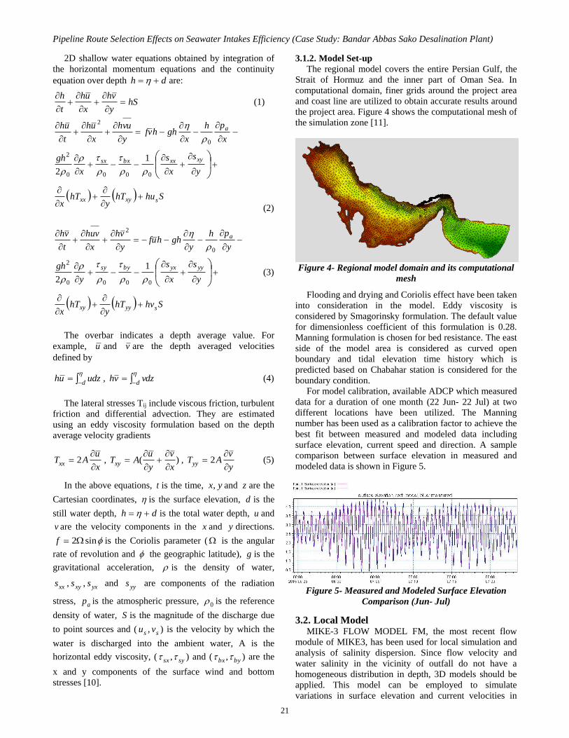
3.1.2. Model Set-up
The regional model covers the entire Persian Gulf, the
Strait of Hormuz and the inner part of Oman Sea. In
computational domain, finer grids around the project area
and coast line are utilized to obtain accurate results around
the project area. Figure 4 shows the computational mesh of
the simulation zone [11].
0:00:00 1899/12/30
Bathymetry [m]
Above -10
-20 - -10
-30 - -20
-40 - -30
-50 - -40
-60 - -50
-70 - -60
-80 - -70
-90 - -80
-100 - -90
-500 - -100
-1000 - -500
-1500 - -1000
-2000 - -1500
-2500 - -2000
-3000 - -2500
Below -3000
Undefined Value
48 49 50 51 52 53 54 55 56 57 58 59 60 61
23.0
23.5
24.0
24.5
25.0
25.5
26.0
26.5
27.0
27.5
28.0
28.5
29.0
29.5
30.0
30.5
Figure 4- Regional model domain and its computational
mesh
Flooding and drying and Coriolis effect have been taken
into consideration in the model. Eddy viscosity is
considered by Smagorinsky formulation. The default value
for dimensionless coefficient of this formulation is 0.28.
Manning formulation is chosen for bed resistance. The east
side of the model area is considered as curved open
boundary and tidal elevation time history which is
predicted based on Chabahar station is considered for the
boundary condition.
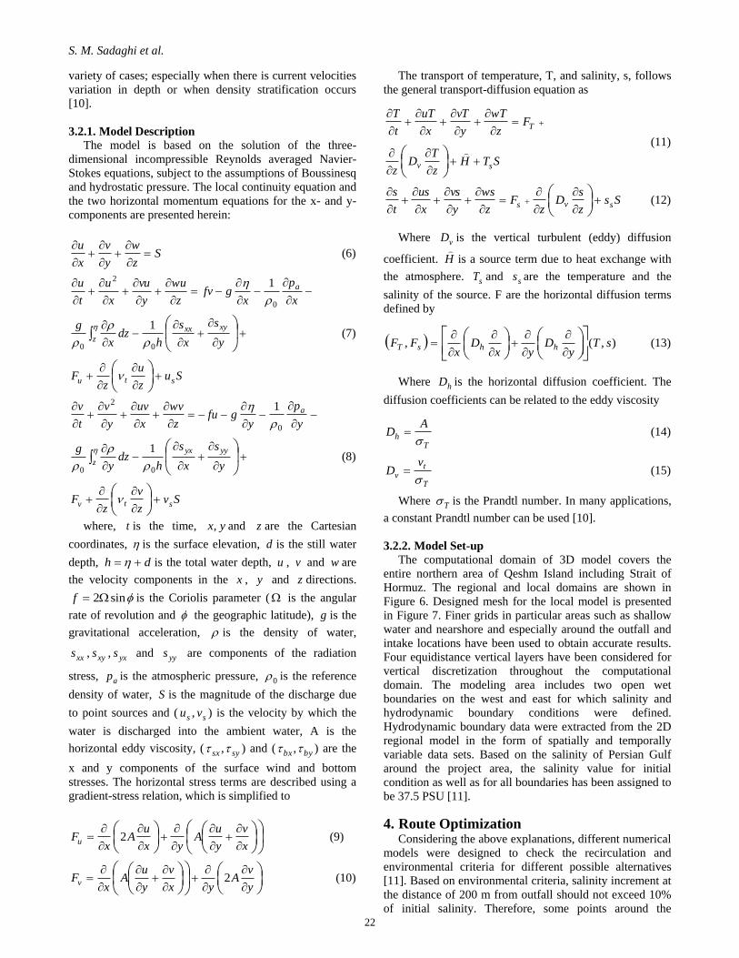
For model calibration, available ADCP which measured
data for a duration of one month (22 Jun- 22 Jul) at two
different locations have been utilized. The Manning
number has been used as a calibration factor to achieve the
best fit between measured and modeled data including
surface elevation, current speed and direction. A sample
comparison between surface elevation in measured and
modeled data is shown in Figure 5.
Figure 5- Measured and Modeled Surface Elevation
Comparison (Jun- Jul)
3.2. Local Model MIKE-3 FLOW MODEL FM, the most recent flow
module of MIKE3, has been used for local simulation and
analysis of salinity dispersion. Since flow velocity and
water salinity in the vicinity of outfall do not have a
homogeneous distribution in depth, 3D models should be
applied. This model can be employed to simulate
variations in surface elevation and current velocities in
S. M. Sadaghi et al.
22
variety of cases; especially when there is current velocities
variation in depth or when density stratification occurs
[10].
3.2.1. Model Description
The model is based on the solution of the three-
dimensional incompressible Reynolds averaged Navier-
Stokes equations, subject to the assumptions of Boussinesq
and hydrostatic pressure. The local continuity equation and
the two horizontal momentum equations for the x- and y-
components are presented herein:
Sz
w
y
v
x
u
(6)
Suz
u
zF
y
s
x
s
hdz
x
g
x
p
xgfv
z
wu
y
vu
x
u
t
u
stu
xyxx
z
a
00
0
2
1
1
(7)
Svz
v
zF
y
s
x
s
hdz
y
g
y
p
ygfu
z
wv
x
uv
y
v
t
v
stv
yyyx
z
a
00
0
2
1
1
(8)
where, t is the time, yx, and z are the Cartesian
coordinates, is the surface elevation, d is the still water
depth, dh is the total water depth, u , v and w are
the velocity components in the x , y and z directions.
sin2f is the Coriolis parameter ( is the angular
rate of revolution and the geographic latitude), g is the
gravitational acceleration, is the density of water,
xxs , xys , yxs and yys are components of the radiation
stress, ap is the atmospheric pressure, 0 is the reference
density of water, S is the magnitude of the discharge due
to point sources and ( ss vu , ) is the velocity by which the
water is discharged into the ambient water, A is the
horizontal eddy viscosity, ( sysx , ) and ( bybx , ) are the
x and y components of the surface wind and bottom
stresses. The horizontal stress terms are described using a
gradient-stress relation, which is simplified to
x
v
y
uA
yx
uA
xFu 2 (9)
y
vA
yx
v
y
uA
xFv 2 (10)
The transport of temperature, T, and salinity, s, follows
the general transport-diffusion equation as
STHz
TD
z
Fz
wT
y
vT
x
uT
t
T
sv
T
(11)
Ssz
sD
zF
z
ws
y
vs
x
us
t
ssvs
(12)
Where vD is the vertical turbulent (eddy) diffusion
coefficient. H
is a source term due to heat exchange with
the atmosphere. sT and ss are the temperature and the
salinity of the source. F are the horizontal diffusion terms
defined by
),(, sTy
Dyx
Dx
FF hhsT
(13)
Where hD is the horizontal diffusion coefficient. The
diffusion coefficients can be related to the eddy viscosity
Th
AD
(14)
T
tv
vD
(15)
Where T is the Prandtl number. In many applications,
a constant Prandtl number can be used [10].
3.2.2. Model Set-up
The computational domain of 3D model covers the
entire northern area of Qeshm Island including Strait of
Hormuz. The regional and local domains are shown in
Figure 6. Designed mesh for the local model is presented
in Figure 7. Finer grids in particular areas such as shallow
water and nearshore and especially around the outfall and
intake locations have been used to obtain accurate results.
Four equidistance vertical layers have been considered for
vertical discretization throughout the computational
domain. The modeling area includes two open wet
boundaries on the west and east for which salinity and
hydrodynamic boundary conditions were defined.
Hydrodynamic boundary data were extracted from the 2D
regional model in the form of spatially and temporally
variable data sets. Based on the salinity of Persian Gulf
around the project area, the salinity value for initial
condition as well as for all boundaries has been assigned to
be 37.5 PSU [11].
4. Route Optimization Considering the above explanations, different numerical
models were designed to check the recirculation and
environmental criteria for different possible alternatives
[11]. Based on environmental criteria, salinity increment at
the distance of 200 m from outfall should not exceed 10%
of initial salinity. Therefore, some points around the

Pipeline Route Selection Effects on Seawater Intakes Efficiency (Case Study: Bandar Abbas Sako Desalination Plant)
23
different assumed outfalls at the distance of 200 m are
selected for checking the environmental criterion.
Figure 6. Regional and local model domains
Figure 7. Mesh generated for 3D local model
In addition, the salinity increment in the intake point
should be negligible. It means that, intake water should not
be affected by salinity plume of outfall. For this purpose,
the salinity increment values at the intake points are
extracted and presented as time series charts. A sample
dispersion pattern for the 3rd alternative is shown in Figure
8 [10, 11].
According to the results, the third alternative was
proved to fulfill both recirculation and environmental
criteria. In this innovative approach, unlike the common
practice, the intake is located closer to the shoreline in
comparison with the outfall point.
A sample of salinity increment time series at intake
point of the third alternative for surface and near bed
locations are shown in Figure 9.
Figure 8. Salinity dispersion pattern for the 3rd
alternative
Figure 9. Salinity increment in surface (top) and near
bed (bottom) at the intake location- alternative 3
The selected alternatives are also evaluated from an
economical perspective. The construction costs of these
alternatives are compared to each other to select the most
optimized route for the pipelines. Cost estimations are
roughly measured by taking into consideration only the
major effective parameters. These parameters include the
costs of procurement and installation of pipelines, dredging

S. M. Sadaghi et al.
24
and backfilling operations. Unit costs for the effective
parameters are assumed based on local experiences, in
order to achieve a rational comparison between the
alternatives.
Considering all the above mentioned aspects, the third
alternative is concluded to be the most optimized choice.
The most notable advantages of this alternative are
summarized below:
Due to the considerable decrease in pipes length
(decrease of about 11250 m HDPE pipes) and
associated dredging volumes, the construction costs
attributed to the optimized route were decreased more
than 25% compared to the initial plan.
The operation and maintenance costs of the third
alternative are much less than the existing plan due to a
major reduction in the total pipeline lengths.
The reduction of intake pipes length decreases the linear
head losses considerably which increases the hydraulic
capacity of pipes and the intake basin.
The increase in the intake capacity in the third
alternative leads to higher system availability and
reliability especially for extreme conditions.
5. Conclusion The present study has shown that the route selection for
submarine pipelines in seawater intake and outfall systems,
has considerable effects on project overall costs and
efficiency. In route selection, different aspects should be
considered simultaneously. In most cases, the shortest
route perpendicular to the coastline is selected for the
pipeline route, but the present study has shown that more
investigation about the optimized route may lead to
considerable improvements in project overall efficiency
and cost benefits. The shortest routes eventuate the lowest
costs but it should be proved to fulfill the required intake
water quality and avoid the recirculation between intake
and outfall. The environmental criteria should also be met
around outfall point. Numerical models are of great use in
selecting the best route which fulfills all the desired
criteria.
6. References [1]. Gille, D. “Seawater intakes for desalination plants”,
Desalination, 156(1–3), 249–256, 2003.
[2]. Cartier, G, & Corsin, P. “Description of different water
intakes for SWRO plants”. In Proceedings of the International
Desalination Association World Congress on Desalination and
Water Reuse, Gran Canaria, Spain, October 21–26, 2007, Paper
IDAWC/MP07-185.
[3]. Hayashi, M., Ikeda, T., Otsuka, K., & Takahashi, M. M.
“Assessment on environmental effects of deep ocean water
discharged into coastal sea”. In: Saxena, N. (ed.) Marine Science
and Technology, PACON International, 535–546, 2003.
[4]. Takahashi, M., & Ikeya, T. “Ocean fertilization using deep
ocean water (DOW)”. Deep Ocean Water Research, 4, 73–87,
2003.
[5]. Takahashi, M., & Yamashita, K. “Clean and safe supply of
fish and shellfish to clear the HACCP regulation by use of clean
and cold water in Rausu, Hokkaido, Japan”. Japan Journal of
Oceanography, 4, 219–223, 2005.
[6]. Takahashi, M., & Huang, P.-Y. “Novel renewable natural
resource of deep ocean water (DOW) and their current and future
practical applications”. Kuroshio Science, 6, 101–113, 2012.
[7]. Pankratz, T., “An Overview of Seawater Intake Facilities for
Seawater Desalination”. CH2M Hill, Inc.
[8]. Pars Geometry Consultants, SAKO Desalination Plant,
“Design general data” report, 2015.
[9]. Iranian Environmental Protection Organization Standard for
effluent disposal, Department of Environment of Iran
[10]. Mike 21 User Manual, Danish Hydraulic Engineering
(DHI), Denmark, 2014
[11]. Pars Geometry Consultants, SAKO Desalination Plant,
“Evaluation of salinity distribution and saline water recirculation”
report, 2015.


