
Resources on quantitative/statistical research for applied ...


Editorial Board
I
JAQM Editorial Board Editors Ion Ivan, University of Economics, Romania Claudiu Herteliu, University of Economics, Romania Gheorghe Nosca, Association for Development through Science and Education, Romania Editorial Team Cristian Amancei, University of Economics, Romania Sara Bocaneanu, University of Economics, Romania Catalin Boja, University of Economics, Romania Irina Maria Dragan, University of Economics, Romania Eugen Dumitrascu, Craiova University, Romania Matthew Elbeck, Troy University, Dothan, USA Nicu Enescu, Craiova University, Romania Bogdan Vasile Ileanu, University of Economics, Romania Miruna Mazurencu Marinescu, University of Economics, Romania Daniel Traian Pele, University of Economics, Romania Ciprian Costin Popescu, University of Economics, Romania Marius Popa, University of Economics, Romania Mihai Sacala, University of Economics, Romania Cristian Toma, University of Economics, Romania Erika Tusa, University of Economics, Romania Adrian Visoiu, University of Economics, Romania Manuscript Editor Lucian Naie, SDL Tridion

Advisory Board
II
JAQM Advisory Board Ioan Andone, Al. Ioan Cuza University, Romania Kim Viborg Andersen, Copenhagen Business School, Denmark Tudorel Andrei, University of Economics, Romania Gabriel Badescu, Babes-Bolyai University, Romania Catalin Balescu, National University of Arts, Romania Constanta Bodea, University of Economics, Romania Ion Bolun, Academy of Economic Studies of Moldova Recep Boztemur, Middle East Technical University Ankara, Turkey Constantin Bratianu, University of Economics, Romania Irinel Burloiu, Intel Romania Ilie Costas, Academy of Economic Studies of Moldova Valentin Cristea, University Politehnica of Bucharest, Romania Marian-Pompiliu Cristescu, Lucian Blaga University, Romania Victor Croitoru, University Politehnica of Bucharest, Romania Cristian Pop Eleches, Columbia University, USA Bogdan Ghilic Micu, University of Economics, Romania Anatol Godonoaga, Academy of Economic Studies of Moldova Alexandru Isaic-Maniu, University of Economics, Romania Ion Ivan, University of Economics, Romania Radu Macovei, University of Medicine Carol Davila, Romania Dumitru Marin, University of Economics, Romania Dumitru Matis, Babes-Bolyai University, Romania Adrian Mihalache, University Politehnica of Bucharest, Romania Constantin Mitrut, University of Economics, Romania Mihaela Muntean, Western University Timisoara, Romania Ioan Neacsu, University of Bucharest, Romania Peter Nijkamp, Free University De Boelelaan, The Nederlands Stefan Nitchi, Babes-Bolyai University, Romania Gheorghe Nosca, Association for Development through Science and Education, Romania Dumitru Oprea, Al. Ioan Cuza University, Romania Adriean Parlog, National Defense University, Bucharest, Romania Victor Valeriu Patriciu, Military Technical Academy, Romania Perran Penrose, Independent, Connected with Harvard University, USA and London University, UK Dan Petrovici, Kent University, UK Victor Ploae, Ovidius University, Romania Gabriel Popescu, University of Economics, Romania Mihai Roman, University of Economics, Romania Ion Gh. Rosca, University of Economics, Romania Gheorghe Sabau, University of Economics, Romania Radu Serban, University of Economics, Romania Satish Chand Sharma, Janta Vedic College, Baraut, India Ion Smeureanu, University of Economics, Romania Ilie Tamas, University of Economics, Romania Nicolae Tapus, University Politehnica of Bucharest, Romania Daniel Teodorescu, Emory University, USA Dumitru Todoroi, Academy of Economic Studies of Moldova Nicolae Tomai, Babes-Bolyai University, Romania Viorel Gh. Voda, Mathematics Institute of Romanian Academy, Romania Victor Voicu, University of Medicine Carol Davila, Romania Vergil Voineagu, University of Economics, Romania

Contents
III
Page
Quantitative Methods in Demographics Mihai Ioan MUTASCU Population Growth and Democracy: An Extreme Value Analyzes in Romania’s Case
259
Md. Jamal UDDIN, Md. Zakir HOSSAIN, Mohammad Ohid ULLAH Child Mortality in a Developing Country: A Statistical Analysis 270 Constanta MIHAESCU, Ileana NICULESCU-ARON, Dana PETRE (COLIBABA) Natality Impact on Recent Demographic Ageing Dynamics in Romania 284
Quantitative Methods Inquires
Muje GJONBALAJ, Marjan DEMA, Iliriana MIFTARI The Role of Statistics in Kosovo Enterprises 295 Ben OBI, Abu NURUDEEN Do Fiscal Deficits Raise Interest Rates in Nigeria? A Vector Autoregression Approach
306
Mostefa BELMOKADDEM, Mohammed MEKIDICHE, Abdelkader SAHED Application of a Fuzzy Goal Programming Approach with different Importance and Priorities to Aggregate Production Planning
317
Marius GIUCLEA, Ciprian POPESCU A Mathematical Deterministic Approach in Modeling National Economic Evolution
332
Zohar LASLO, Hagai ILANI, Baruch KEREN A Lower Bound for Project Completion Time Attained by Detailing Project Tasks and Redistributing Workloads
344
Software Analysis
Marius POPA, Cristian TOMA Stages for the Development of the Audit Processes of Distributed Informatics Systems
359
Lorena BATAGAN, Adrian POCOVNICU, Sergiu CAPISIZU E-Service Quality Management 372 Marinela MIRCEA, Anca ANDREESCU Using Business Rules in Business Intelligence 382 Paul POCATILU, Cristian CIUREA Collaborative Systems Testing 394

Quantitative Methods in Demographics
259
POPULATION GROWTH AND DEMOCRACY: AN EXTREME VALUE ANALYZES IN ROMANIA’S CASE
Mihai Ioan MUTASCU1 PhD, Associated Professor, Economics and Business Administration Faculty, West University of Timisoara, Romania E-mail: [email protected], [email protected]
Abstract: The paper analyzes empirically, in Romania’s case, the relationships between population growth (dependent variable) and the dimensions of democracy (independent variables). The analysis is based on the construction of a linear “Extreme Value Model”. In Romania’s case, the probability of annual population growth to be more then 10.000 persons could be high, if the state is a dictatorial monarchy, the political regime durability is high and the abort is legal. In such conditions, the type of political regime and the abort restrictions are brought forward by the democratization intensity and political regime durability. In other words, the main results show that, in Romania’s case, the probability of annual population growth to be more then 10.000 persons could be high, if the level of democratization intensity is low and the political regime durability is high. Key words: population growth; democracy; factors; connections; extreme value analysis
1. Introduction
The population growth represents the change in the level of population over the time. These modifications are caused by several factors, with different action intensity. During the last years, the conceptualization of the population growth was different, but in essence they reflect the same idea. In a minimal view, the main factors which have a direct impact on population growth consist in fertility, mortality and migration (Alho and Spencer, 1985). Moreover, for the authors, these three factors illustrate the major source of errors in forecasts of the total population in the United States. In a limitative sense, other opinions resume that the population growth goes hand in hand with economic development (Jackson, 1995).
The determinants of population growth, in other vision, could be: the availability of sparsely populated areas, the industrial revolution, the revolution in transport of food and goods, the medical revolution; and the green revolution (Mostert, Oosthuizen, Hofmeyr and Zyl, 1998). Some studies are focalized on the relationship between population growth and

Quantitative Methods in Demographics
260
political regime and include both directions of putative causation: how demographic change affects politics, and how political forces affect demographic patterns (Teitelbaum, 2005).
In an extended version, the population growth determinants have two directions: one, that groups the health demographic factors, such as child mortality, immunizations, nutrition, HIV/AIDS, access to healthcare and maternal mortality, and another one, that summarizes the socioeconomic demographic factors, such as economy, education, age composition, total fertility rate, orphans and child labor (Casper and Kitchen, 2008).
In our opinion, all these scientific acquisitions bring to the remark that population growth has in fact two main categories of determinants: one exogenous and another endogenous.
On the one hand, the exogenous determinants of the population growth have an indirect impact and include: the economic conditions, the health care system, the education, the political regime; the rule of laws, the culture; and so on. On the other hand, the endogenous factors of the population growth refer to the determinants, such as the fertility, the mortality and the migration, with a direct impact.
All of them have a significant impact on the population growth, but the field literature offers different points of view regarding “the sign” of this relationships.
2. Theoretical fundaments
Between exogenous determinant factors of population growth, the democracy, as political factor, has an important role, even if the field research offers few studies. No matter how, the impact of democracy on population growth could be focused both on intensity of democratization and political regime durability one.
According to the first coordinates - the intensity of democratization, the results reveal that the population growth is faster under dictatorship than under democracy (Handenius, 1997). In the same note, the population growth is faster under dictatorships in all but one income band, poor countries differ little regardless of regimes, and the rate of domestic population growth falls faster as income increases in wealthier democracies than in wealthier dictatorships (Przeworski, Alvarez and Cheibub, 2000).
Moreover, in connection with economic development, population grows faster under dictatorships and per capita incomes increase more rapidly under democracies (Przeworski, 2000). Another author shows that the degree of democracy or political freedom also has a dampening effect on population growth (Feng, 2005). Regarding the interaction between the population change with the democracy and the power status indicator variables, the effect of population growth is clearly evident for the democratic minor powers (Cranmer and Siverson, 2008).
On the contrary, other results show a positive effect of democracy on economic growth over time, with a significant mediating role for fertility (Roberts, 2006). More precisely, the growth of population is faster, as the level of democratization is increasing.
For the second coordinates - the political regime durability, the scientific acquisitions illustrate that the fertility decisions are determined by three fundamental political variables: political stability, political capacity and political freedom (Feng, Kugler and Zak, 1999). The same authors, in an empirical study in China’s case, argue that political stability and government capacity are two crucial factors that shape family decisions regarding the number of children (Feng, Kugler and Zak, 2002). In the same note, political

Quantitative Methods in Demographics
261
stability also reduces birth rates; more precisely, population growth is faster as the intensity of political regime durability is higher (Feng, 2005).
Therefore, the researches on the causal relationship’s sign between population growth and its democratic determinants are not conclusive; some of them claim the connections of the same sign and other of the contrary sign.
This scientific approach is intended to analyze, in Romania’s case, the relationship between population growth and its democratic determinants. According to the mentioned premise, all the theoretical elements presented allow us to formulate a series of theoretical working assumptions, which consider two of the main characteristics of democracy: intensity of democratization and political regime durability.
The assumptions hypotheses are: H1: The population growth is faster as the intensity of democratization is smaller. H2: The population growth is faster as the political regime durability is higher.
In summary, the meanings of the hypothesis’ work relations are: Table 1. The sense („the sings”) of the hypothesis’ work relations
The trend of population growth
The main democratic factors of population growth
The trend of democratic factors of population growth
+ Intensity of democratization - + Political regime durability +
The fundamental assumption is that population growth represents a complex
demographic phenomenon, determined by a couple of exogenous factors, especially political regime.
3. Methods and results
Starting with the theoretical argues shown, the paper analyzes empirically, in Romania’s case, the relationships between the population growth (dependent variable) and its exogenous political factors (independent variables). The analysis is based on the construction of a linear “Extreme Value Model” and the data set is covering the period 1926-2007.The measures of democracy and its determinants are presented in Table 2.
Moreover, I entered two sets of dummy variables. The first set, considers dummy variable - TG, which reflects the form of government
(monarchy or republic). If the state is a monarchy, the dummy is 1, and if the state is a republic, dummy is 0 (in Romania, in the considered sample, the monarchic period covers the interval 1926-1947). In a monarchy, in a democratic approach, the most important function is to sustain the legitimacy of the state. More, under modern conditions, a constitutional monarchy serves not to limit democracy but to underpin and indeed to sustain it (Bogdanor, 1997).
The second set, considers dummy variable - A, which reflects the freedom of abortion. If abortion is legal, the dummy is 1, and if abortion is illegal, dummy is 0 (in Romania, in the considered sample, the abortion has been illegal in two periods: from 1923 to 1955; and from 1966 to 1990).

Quantitative Methods in Demographics
262
Table 2. The variables’ description and its sources
Variable Measure and description Source
Population growth - PG
Population Growth represents the difference between the numbers of total population in a country for two consecutive years.
Statistical Yearbook of Romania, National Institute of Statistics, 1927 -2008
Level of democracy -DE
Index of Democratization illustrates the rank of democracy’s level (intensity of democratization).
Vanhanen (2007)
Political regime durability - D
Political regime durability represents the number of years since the most recent regime change or the end of transition period defined by the lack of stable political institutions.
Madison (2003)
Form of government - TG
Dummy variables reflect the form of government (monarchy - 1 or republic - 0).
Dummy methodology
Freedom of abort - A
Dummy variables reflect freedom of abort (legal abort - 1 or illegal abort - 0).
Dummy methodology
Because some of the considered independent factors (DE and D) have different scales
of measurement, for a comparative analysis, the levels of variables were normalized:
..
.
MinMax
MinNormalized IFIF
IFIFIF
−−
= (1)
where IF represents the independent variables DE and D.
[ ]1,0∈NormalizedIF (2)
In this case, DE and D become DEMO and DM, where 0 corresponds to the
minimum intensity level of indicators and 1 indicates the maximum intensity level. Population Growth (PG) has different absolute levels over the years:
1−−= tt NPNPPG (3)
where NP illustrates the number of total population in a country in the year t. In our extreme value approach, the Population Growth becomes “The Probability of
Annual Population Growth to be more then 10.000 Persons” - P:
⎩⎨⎧
≥<
=10.000PG if 1,10.000PG if
P,0
(4)
Based on the theoretical assumptions made above and on the normalized
illustrated variables, the sense of the relationship between “The Probability of Annual Population Growth to be more then 10.000 Persons” and its considered determinant factors as it follows:

Quantitative Methods in Demographics
263
Table 3. The expected sense („the sings”) of the relations between P - DEMO, DM, TG and A
The Probability of Annual Population Growth to be more then 10.000 Persons
The main democratic factors of population growth
The trend of democratic factors of population growth
+ DEMO - + DM + + TG + or - + A -
In extreme value estimation one hypothesis that the probability p of the occurrence
of the event is determined by the function:
)iZe-i(Z expiZFip == )( for ∞<<∞− Z (5)
where Z is a linear function of the explanatory variables.
The marginal effect of Z on the probability, which will be denoted f(Z), is given by the derivative of this function with respect to Z:
dZdpZf =)( (6)
In extreme value analysis the marginal effect of Z on the probability is not constant. It
depends on the value of f(Z), which, in turn, depends on the values of each of the explanatory variables. To obtain a summary statistic for the marginal effect, the usual procedure is parallel to that used in extreme value analysis, based on the mean values of the explanatory variables.
In the considered case, Z is:
εββββα +++++= iiii xAxTGxDMxDEMOZ 4321 (7)
where α are the intercept term and i is the period of time (years 1926-2007).
From 82 included P observations, 26% are 0 (The Probability of Annual Population Growth to be more then 10.000 Persons is null) and 73% are 1 (The Probability of Annual Population Growth to be more then 10.000 Persons is positive): Table 4. The P frequencies, in Romania, in the period 1926-2007
Dependent Variable: P Method: ML - Binary Extreme Value (Newton-Raphson) Date: 07/05/09 Time: 19:56 Sample: 1926 2007
Included observations: 82 Frequencies for dependent variable Cumulative
Value Count Percent Count Percent 0 22 26.00 22 26.83 1 60 73.00 82 100.00

Quantitative Methods in Demographics
264
The econometric tests of the “Extreme Value Model” are: Table 5. The econometric tests of the “Extreme Value Model P - DEMO, DM, TG and A”
Dependent Variable: P
Method: ML - Binary Extreme Value (Newton-Raphson)
Date: 07/09/09 Time: 01:28
Sample: 1926 2007
Included observations: 82
Convergence achieved after 5 iterations
GLM Robust Standard Errors & Covariance
Variance factor estimate = 0.6996205118
Covariance matrix computed using second derivatives Variable Coefficient Std. Error z-Statistic Prob. DEMO -4.129881 1.330049 -3.105059 0.0019
DM 6.615952 1.531099 4.321049 0.0000
TG 0.919438 0.416760 2.206157 0.0274
A 0.893263 0.754669 1.183650 0.2366 Mean dependent var 0.731707 S.D. dependent var 0.445797
S.E. of regression 0.323706 Akaike info criterion 0.694619
Sum squared resid 8.173281 Schwarz criterion 0.812020
Log likelihood -24.47939 Hannan-Quinn criter. 0.741754
Avg. log likelihood -0.298529 Obs with Dep=0 22 Total obs 82
Obs with Dep=1 60
The tests of the model show that the absolute values of the standard errors
corresponding to the coefficients of the function are lower than the values of the coefficients; witch sustains the correct estimation of these coefficients (a conclusion reinforced by the low values of the probabilities). For more accuracy, the model considers a robust covariance GLM and Newton-Raphson optimization algorithm.
Based on the model, the expectation-prediction values are: Table 6. The expectation-prediction values of “Extreme Value
Model P - DEMO, DM, TG and A”
Dependent Variable: P
Method: ML - Binary Extreme Value (Newton-Raphson)
Date: 07/09/09 Time: 01:33
Sample: 1926 2007
Included observations: 82
Prediction Evaluation (success cutoff C = 0.5)
Estimated Equation Constant Probability
Dep=0 Dep=1 Total Dep=0 Dep=1 Total
P(Dep=1)<=C 18 7 25 0 0 0
Quantitative Methods in Demographics
265
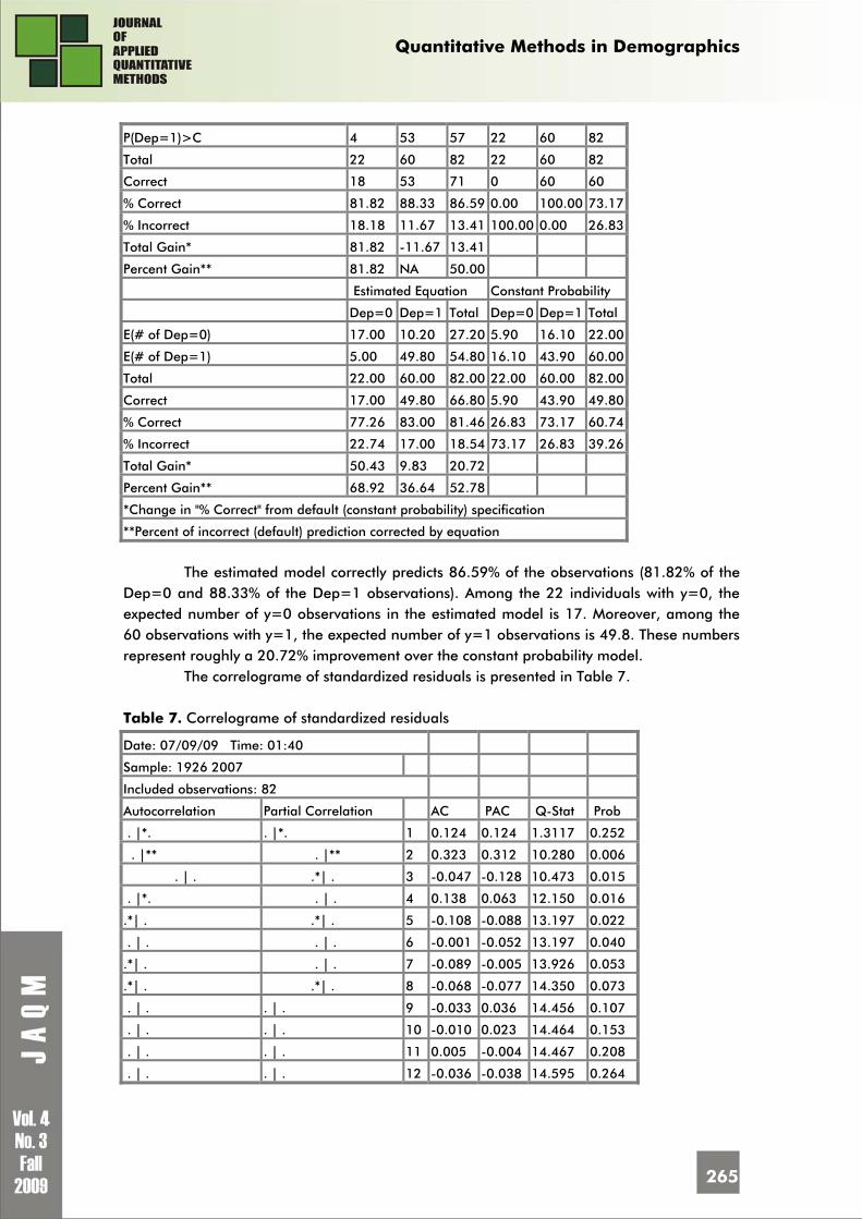
P(Dep=1)>C 4 53 57 22 60 82
Total 22 60 82 22 60 82
Correct 18 53 71 0 60 60
% Correct 81.82 88.33 86.59 0.00 100.00 73.17
% Incorrect 18.18 11.67 13.41 100.00 0.00 26.83
Total Gain* 81.82 -11.67 13.41
Percent Gain** 81.82 NA 50.00
Estimated Equation Constant Probability
Dep=0 Dep=1 Total Dep=0 Dep=1 Total
E(# of Dep=0) 17.00 10.20 27.20 5.90 16.10 22.00
E(# of Dep=1) 5.00 49.80 54.80 16.10 43.90 60.00
Total 22.00 60.00 82.00 22.00 60.00 82.00
Correct 17.00 49.80 66.80 5.90 43.90 49.80
% Correct 77.26 83.00 81.46 26.83 73.17 60.74
% Incorrect 22.74 17.00 18.54 73.17 26.83 39.26
Total Gain* 50.43 9.83 20.72
Percent Gain** 68.92 36.64 52.78
*Change in "% Correct" from default (constant probability) specification
**Percent of incorrect (default) prediction corrected by equation
The estimated model correctly predicts 86.59% of the observations (81.82% of the
Dep=0 and 88.33% of the Dep=1 observations). Among the 22 individuals with y=0, the expected number of y=0 observations in the estimated model is 17. Moreover, among the 60 observations with y=1, the expected number of y=1 observations is 49.8. These numbers represent roughly a 20.72% improvement over the constant probability model.
The correlograme of standardized residuals is presented in Table 7. Table 7. Correlograme of standardized residuals
Date: 07/09/09 Time: 01:40
Sample: 1926 2007
Included observations: 82
Autocorrelation Partial Correlation AC PAC Q-Stat Prob
. |*. . |*. 1 0.124 0.124 1.3117 0.252
. |** . |** 2 0.323 0.312 10.280 0.006
. | . .*| . 3 -0.047 -0.128 10.473 0.015
. |*. . | . 4 0.138 0.063 12.150 0.016
.*| . .*| . 5 -0.108 -0.088 13.197 0.022
. | . . | . 6 -0.001 -0.052 13.197 0.040
.*| . . | . 7 -0.089 -0.005 13.926 0.053
.*| . .*| . 8 -0.068 -0.077 14.350 0.073
. | . . | . 9 -0.033 0.036 14.456 0.107
. | . . | . 10 -0.010 0.023 14.464 0.153
. | . . | . 11 0.005 -0.004 14.467 0.208
. | . . | . 12 -0.036 -0.038 14.595 0.264

Quantitative Methods in Demographics
266
The tests show that there are some “low” autocorrelations and partial correlations of standardized residuals for inferior lags (especially for lag 2). The fact is explicable because all of five data series are not provided by the same source. However, we consider that this impediment does not affect the quality and stability of the model.
Moreover, the high value of Andrews Goodness-of-Fit Test and low level of Hosmer-Lemeshow Goodness-of-Fit Test does not suggest the caution in interpreting of the results (Table 8).
Table 8. Andrews and Hosmer-Lemeshow Goodness-of-Fit Tests
Dependent Variable: P Method: ML - Binary Extreme Value (Newton-Raphson) Date: 07/09/09 Time: 21:03 Sample: 1926 2007 Included observations: 82 Andrews and Hosmer-Lemeshow Goodness-of-Fit Tests Grouping based upon predicted risk (randomize ties) Quantile of Risk Dep=0 Dep=1 Total H-L Low High Actual Expect Actual Expect Obs Value 1 9.E-12 0.0021 8 7.99706 0 0.00294 8 0.00294 2 0.0518 0.2211 5 6.96587 3 1.03413 8 4.29193 3 0.2227 0.3430 4 5.72435 4 2.27565 8 1.82602 4 0.4054 0.6712 2 3.23729 6 4.76271 8 0.79432 5 0.6712 0.8947 3 1.99572 6 7.00428 9 0.64936 6 0.9072 0.9447 0 0.56318 8 7.43682 8 0.60583 7 0.9465 0.9643 0 0.35371 8 7.64629 8 0.37007 8 0.9661 0.9764 0 0.22560 8 7.77440 8 0.23214 9 0.9795 0.9932 0 0.10186 8 7.89814 8 0.10318 10 0.9941 0.9984 0 0.03041 9 8.96959 9 0.03052 Total 22 27.1951 60 54.8049 82 8.90631 H-L Statistic: 8.9063 Prob. Chi-Sq(8) 0.3503 Andrews Statistic: 53.2346 Prob. Chi-Sq(10) 0.0000
In conclusion, the model may be considered representative and stabile to describe,
in Romania’s case, the connection between P and DEMO, DM, TG & A.
4. Conclusions
The method for identifying the effect of the DEMO, DM, TG and A on the P consists in calculating the marginal effect at the mean value of the explanatory variables. The next table shows the marginal effects, calculated by multiplying f(Z) with the estimated coefficients of the extreme value regression. Table 9. The marginal effects of the “Extreme Value Model P - DEMO, DM, TG and A”
Variable Mean β Mean × β f(Z) β x f(Z)
DEMO 0.197461 -4.12988 -0.81549 0.041775 -0.03407 DM 0.320826 6.615952 2.12257 0.041775 0.088671 TG 0.268293 0.919438 0.24668 0.041775 0.010305 A 0.341463 0.893263 0.30502 0.041775 0.012742 Total 1.5537578

Quantitative Methods in Demographics
267
Starting from the marginal effects measured on the “extreme value model” built, we can identify the following remarks in Romania’s case:
• an one-point increase in the DEMO, decreases with 3.40% the probability of annual population growth to be more then 10.000 persons;
• an one-point increase in the DM, increases with 8.86% the probability of annual population growth to be more then 10.000 persons;
• an one-point increase in the TG, increases with 1.03% the probability of annual population growth to be more then 10.000 persons;
• an one-point increase in the A, increases with 1.27% the probability of annual population growth to be more then 10.000 persons.
We can observe that the results confirm all the assumption hypotheses, except the freedom of abortion. In such conditions, the model disaffirms only the acquisitions of Roberts (2006), regarding the connection between population growth and democratization.
For the analyzed period, in Romania’s case, a decrease in the level of democratization, an augmentation of political regime durability, with a freedom of abortion, on a monarchical base, increases the probability of annual population growth to be more then 10.000 persons. On the contrary, an augmentation in the level of democratization, a decrease of political regime durability, without the freedom of abortion, on a republican base, decreases the probability of annual population growth to be more then 10.000 persons.
Among the four determinant factors (DEMO, DM, TG and A), the most important one is the political regime durability, followed by the level of democratization. These two factors are followed, in order, by the freedom of abortion and the form of government (monarchy or republic).The forecast of the probability of annual population growth to be more then 10.000 persons, in the period 1926-2007, in Romania, is illustrated in the following graphic:
-4
-2
0
2
4
6
8
1930 1935 1940 1945 1950 1955 1960 1965 1970 1975 1980 1985 1990 1995 2000 2005
The probability of annual population growth to be more then 10.000 persons
Graphic 1. The forecast of the probability of annual population growth to be more then
10.000 persons, in Romania, in the period 1926-2007

Quantitative Methods in Demographics
268
Based on the obtained forecast probability, we can observe four principal intervals of analysis.
The first three intervals have some „strong positive shocks” (the probability of annual population growth to be more then 10.000 persons is high): from 1939 to 1940 - the dictatorship of King Carol II; from 1940 to 1944 - the National Legionary State, in which power was taken by dictator Ion Antonescu; and from 1965 to 1989 - the communist dictatorship of Ceausescu Nicolae. Also, the positive effect on the probability is sustained by political factors, even if the abort has been illegal in two relative large periods: from 1923 to 1955; and from 1966 to 1990.
The last interval, from 1990 to 2007, implies a “strong negative shock” (the probability of annual population growth to be more then 10.000 persons is very low), especially beginning with 1992, the year of the first free democratic elections.
According to the democratic factors strictly, in Romania’s case, the probability of annual population growth to be more then 10.000 persons can be high, if the state is a dictatorial monarchy, the political regime durability is high and the abortion is legal. In such conditions, the type of political regime and the abortion restrictions are brought forward by the democratization intensity and political regime durability. In other words, the main results show that, in Romania’s case, the probability of annual population growth to be more then 10.000 persons can be high, if the level of democratization intensity is low and the political regime durability is major.
References 1. Alho, J. and Spencer, B. Uncertain Population Forecasting, Journal of the American Statistical
Association, Vol. 80, No. 390, 1985, pp.310-312 2. Bogdanor, V. The Monarchy and the Constitution, Oxford University Press, 1997, p.64 3. Casper, L. and Kitchen, P. Demographic Factors, Encyclopedia of Infant and Early Childhood
Development, Elsevier Inc., 2008, pp. 345-356 4. Cranmer, S. and Siverson, R. Demography, Democracy and Disputes: The Search for the
Elusive Relationship Between Population Growth and International Conflict, The Journal of Politics, No.70, Cambridge University Press , 2008, pp. 794-806
5. Feng, Y. Democracy, governance and economic performance, MIT Press, 2005, p. 278 and p. 298
6. Feng, Y., Kugler, J. and Zak, P. Population Growth, Urbanisation and the Role of Government in China: A Political Economic Model of Demographic Change, Urban Studies, Vol. 39, No. 12, 2002, p. 1
7. Feng, Y., Kugler, J. and Zak, P. The path to prosperity: a political model of demographic change, Claremont Colleges Working Papers in Economics, 1999, p. 1
8. Handenius, A. Democracy’s victory and crisis, Cambridge University Press, 1997, p. 172 9. Jackson, W. Population growth. A comparison of evolutionary views, International Journal of
Social Economics, Vol. 22, No. 6, 1995, p. 3 10. Maddison, A. Historical Statistics for the World Economy: 1-2003 AD, Horizontal file,
Copyright Angus Maddison, 2009 11. Mostert, W., Oosthuizen, J., Hofmeyr, B. and Zyl, J. Demography: Textbook for the South
African Student , Human Sciences Research Council Press, 1998, p. 13 12. Przeworski, A., Alvarez, M. and Cheibub, J.A. Democracy and development, Cambridge
University Press, 2000, p. 224 13. Przeworski, A. Democracy and Economic Development, Political Science and the Public
Interest, Ohio State University Press, 2000, p. 1

Quantitative Methods in Demographics
269
14. Roberts, W. Political Regimes as Demographic Regimes: Unpacking the Democracy - Economic Growth Relationship, Paper presented at the Annual Meeting of the American Sociological Association, Montreal Convention Center, Montreal, Quebec, Canada, 2006, p. 1
15. Teitelbaum, M. Political Demography, Handbooks of Sociology and Social Research, Springer Publisher, 2005, p. 719
16. Vanhanen, T. Introduction: Measures of Democratization, Finnish Social Science Data Archive, 2007, pp. 20-21
17. * * * World Economic Outlook Database, International Monetary Fund, April 2009 18. * * * Statistical Yearbook of Romania, National Institute of Statistics, 1927-2008
1Mihai Mutascu is assistant professor at West University of Timisoara, Faculty of Economic and Business Administration and teaches public finance, public economics and taxation. From 2005 is collaborator of National Institute for Administration, when teaches public policy and local public finance. His main areas of interest are public finance, fiscal federalism and public choice. From 2006 is member of Public Choice Society, Center for Study of Public Choice, George Mason University, Fairfax, Virginia, USA.

Quantitative Methods in Demographics
270
CHILD MORTALITY IN A DEVELOPING COUNTRY: A STATISTICAL ANALYSIS
Md. Jamal UDDIN1,2 MSc, University Lecturer, Department of Statistics, Shahjalal University of Science & Technology, Sylhet, Bangladesh E-mail: [email protected], [email protected]
Md. Zakir HOSSAIN3 PhD, University Professor, Department of Statistics, Shahjalal University of Science & Technology, Sylhet, Bangladesh E-mail: [email protected] Mohammad Ohid ULLAH4 MSc, Assistant Professor, Department of Statistics, Shahjalal University of Science & Technology, Sylhet, Bangladesh E-mail: [email protected]
Abstract: This study uses data from the “Bangladesh Demographic and Health Survey (BDHS] 1999-2000” to investigate the predictors of child (age 1-4 years] mortality in a developing country like Bangladesh. The cross-tabulation and multiple logistic regression techniques have been used to estimate the predictors of child mortality. The cross-tabulation analysis shows that parents’ education is the vital factor associated with child mortality risk but in logistic regression analysis only the father’s education has been found significant to reducing child mortality. Occupation of father has been found a significant characteristic in both analyzes, further mother standard of living index, breastfeeding status, birth order has substantial impact on child mortality in Bangladesh. The findings also show that in both statistical analyzes maternal health care variables such as timing of first antenatal check and tetanus toxoid (TT] during pregnancy has momentous effect on child mortality. Finally these findings specified that an increase in parents’ education, improve health care services which should in turn raise child survival and should decrease child mortality in Bangladesh. Key words: Neonatal; Post-neonatal; Tetanus Toxoid; SLI

Quantitative Methods in Demographics
271
Introduction The study of child mortality becomes one of the most important researches of the
developing countries including Bangladesh. There are two major reasons behind this: (i] high level of infant & child mortality and (ii] its relationship with fertility. The reduction of infant and child mortality indirectly helps in reducing fertility by decreasing the desired number of children to be born due to increased probability of survival of a child. The child mortality is a composite index reflecting environmental, social, economic, health care services and delivery situation on the one hand and maternal as well as family and community norms and practices on the other.
A child is highly vulnerable to two categories of acquired ailments; one is a heavy load of infectious diseases and the other, those diseases that are caused by inadequate nutrition. The relationship between child mortality and socio-economic factors might be relatively weak in developed countries, may be due to low child mortality. In contrast, in the developing countries, a significant portion of deaths occurs during childhood, which may be due to poor public health measures and lack of access to health care facilities. It is documented that the risk of morbidity and mortality is directly influenced by 14 intermediate or proximate determinates including education of mother, sanitation facilities, access to safe drinking water and maternal and child health care services (38). There is evidence of some recent decline in infant and child mortality. Mother education, higher birth order had significant independent effects upon the reduction of infant and child mortality. Other variables such as father education, fetal loss or land ownership had no effect on child mortality [3]5. Another study considers some characteristics as mother’s age at the birth of child, birth order, previous child loss, mother’s residence, father’s occupation and mother’s work experience since marriage [1].
Maternal education has been observed strong predictor of child mortality in developing countries [6, 10, 15, 21, 28, 33, 41]. The education of the mother is emerged as one of the strongest predictors of child mortality though other factors like women’s autonomy, income, working status of parents, standard of living index, household size, place of residence, better conditions of water supply and sanitation have influence upon it [26, 20, 43]. Some studies indicated that the mother’s education is a more decisive determinant of child survival than other family characteristics such as father’s occupation and father’s education [2, 10]. Mother’s education may be attributed to the children of enjoying better diets and better overall care than the children of non-educated mothers [4] and there are strong inverse relationship between mother’s education and child mortality [21, 31]. Another study also identified that mother-working status exerts a significant negative influence on child mortality. But mother education has a greater influence on child survival in Bangladesh than that of father’s education [32].
Few studies have focused on the health and survival of children who migrate from rural areas or who are born to migrants in urban areas of developing countries, although several studies have incorporated maternal migrant status as an explanatory variable on child mortality [9, 19]. In many societies religious differentials have significant impact on child mortality such as the BFS [1989] data indicated that Hindus have a higher child mortality rate than Muslims [30].
Investigations on historical and modern third world countries have shown that children who were exclusively breast-fed survive longer and are healthier than artificially fed

Quantitative Methods in Demographics
272
children in direct proportion [16, 27]. The child mortality causes the cessation of breastfeeding, thus increasing the probability of return to ovulation, so also the conception of the next child, resulting in a shortened birth interval. The strength of this effect is found to be related to the intensity, frequency and duration of breastfeeding [22]. In developing countries including Bangladesh, mother’s age at birth played an important role in child mortality. A number of studies deal with mother’s age at the birth of the child [5, 13, 24] and the optimal ages of child bearing is confined of 20 to 34. It will help to reduce maternal mortality and childhood mortality [44]. Birth interval played significant role on infant and child mortality [23, 35, 39] and the length of the birth interval is short the probability of dying is very high. The probability of dying before age five for children born less than two years after a previous birth is more than double than for those children born four or more years after a previous birth [25]. There are three mechanisms about short birth interval such as –(i) short birth intervals can relate fetal growth resulting in low birth weight and increased death risks due to endogenous causes. (ii) they may impair the potential milk production for the child whose birth closed the intervals. (iii) too closely spaced birth on the distribution of resources increasing maternal care among children in the household [40]. Children through out the developing countries are much more likely to die if they are born less than two years after the mother’s previous birth than their birth interval is longer [23]. Another study observed that in first pregnancies the childhood mortality is highest, in 2nd and 3rd pregnancies that are lowest [12, 34]. A study have used ICDDR’B data for the period October 1975 to January 1980 and identified that 60% to 80% children died in the first two years of life whose birth interval was 15 months with preceding birth [35]. The short birth interval is a risk factor with some qualifications. For example, the bad affect of short birth intervals on child mortality may be reduced by favourable socio-economic conditions [8].
Sex discrimination in infant and child mortality was studied by many researchers [7]. The rural areas of western south Asia, stretching across Pakistan and the northern states of India to Bangladesh, female child death rates are often very much higher in early ages [18]. In few developing countries such as South Asian countries, the Middle East and Northern Africa, it has been observed the excess female mortality during infancy and childhood [45]. The higher mortality rates during childhood period are consistent with overpowering event that biological risk of male is higher than female. The study also examined that male children got more advantages than female in parental care, feeding patterns, intra family food distribution and treatment of illness [12].
In a rural community of Bangladesh, the under five death occurred for most significant causes such as diarrhorea and dysentery, tetanus, measles, fever, respiratory and dropsy [11]. The health care services including higher coverage with immunization, safe delivery of birth is more developed in urban area than rural area in Bangladesh [14, 30]. The availability of adequate health service may bring the mortality rate significantly down for the children aged between 1-4 years, but various social and cultural biases in the population keep them away from using such services and ultimately neutralize the supposed potentials of health service facilities [17]. The number of antenatal care visit and timing of the first antenatal check-up are considered as important factors in preventing an adverse pregnancy outcome. Maternal health care is most effective if the visits are started early stage during pregnancy and continue at regular intervals throughout the pregnancy [37]. The prenatal management, maternal age, maternal nutrition, the process of child birth, treatment of obstetric emergencies played an important role in improving child survival [42]. In

Quantitative Methods in Demographics
273
developing countries women face many health risks that associated with sexuality and child bearing [29] and in Bangladesh, the lack of health care service for mothers is one of the important reasons for the high rates of infant and child mortality [30]. The proper medical attention and hygienic conditions during delivery can reduce the risk of infections and facilitate management of complications that can be caused death or various illnesses for the mother or the newborn child [36].
The review of the literature of child mortality showed that a number of variables affecting child mortality. However, the predictors of child mortality are changing through time since the facilities and awareness are changing day by day. Hence it is necessary to give more emphasis on using the current data to identify the segment of population where programmes need to be strengthening in order to achieve the goal for reducing child mortality.
Objective of the Study In this study an attempt has been made to examine the predictors of child mortality
in Bangladesh. The specific objectives of this study are: to identify the factors which is affecting child mortality and to suggest viable strategies to increase health service and reduce child mortality in Bangladesh.
Data and methods This study uses data from the Bangladesh Demographic and Health Survey [BDHS]
conducted in November 1999 to March 2000 under the authority of the National Institute of Population Research and Training [NIPORT]. The BDHS is intended to serve as a source of population and health for policy makers and research community. The BDHS (1999-2000) is a nationality representative survey of 10544 ever-married women aged 10-49 and 2556 currently married men aged 15-59. The sample has been taken 5 years prior to BDHS (1999-2000) survey. That means, in this study all birth considered between November 1994 to October 1999 and deaths considered between November 1994 to October 1999 and with age 12 months and above.
The interlinkage between child mortality and socio-economic, bio-demographic and maternal health care variables have been tested by applying cross-tabulation analysis. The cross-tabulation analysis is an important in first step for studying the relationship between mortality with several characteristics. However, such analyses fail to address mortality predictors completely because of ignoring other covariates. Hence multiple logistic regression approach is also adopted in order to estimate independent effects of each variable while controlled for others. Multiple logistic regression analysis is carried out for the child according to the age at death. This analysis considered all the covariates that were found significant in cross-tabulation analysis.
Variables: education of mother, education of father, occupation of mother,
occupation of father, religion, family size, exposure to mass media, standard of living index, place of residence, breastfeeding status, birth order, sex of child, birth spacing with previous child, mother age at birth of child, complication during birth, type of birth, timing of first

Quantitative Methods in Demographics
274
antenatal check during pregnancy, TT during pregnancy, number of antenatal visit during pregnancy, place of delivery.
Results and Discussion In this section, we examine the predictors of child mortality. Child mortality reflects a
country’s level of socio-economic development and quality of life. Bangladesh has witnessed a large decline in child mortality during the last two decades [37]. The child mortality varies according to socio-economic, health care and bio-demographic characteristics of the population concerned. There are many predictors of child mortality in a particular group of variables and it is necessary to analyze them separately in order to get the idea about the insight variation of that particular type of variables.
The distribution of child mortality by socio-economic, bio-demographic, and maternal health care variables is shown in Table 1 (Appendix 1). Among socio-economic variables, maternal education has a strong relationship with child mortality and child survival. Various studies have supported a direct causal relationship between mother’s education and child mortality [26, 28, 29]. The result indicates that the child mortality rate was highest (1.64%) for the children of illiterate mothers and lowest (0.54%) for the children whose mother’s educational level is secondary and above. It is clear that the child mortality rate decreases with the increase of mother’s education. Like mother’s education, father’s education also plays significant role on child mortality. Father’s level of education has been regarded as a valid proxy of income and wealth status of the household in Bangladesh. It is likely that higher educated people belong to higher economic class. An investigation of the Table reflects that among the total deaths, highest number of deaths (63.3%) is observed for the illiterate father and the lowest number of deaths (3.8%) is observed for the father whose educational level is H.S.C and above. The child mortality rate was also found highest (1.71%) among the children whose father is illiterate and the child mortality was found lowest (0.43%) for the children whose father’s education is secondary and above. This result shows that child mortality sharply decreases as the father’s educational level increases. So it may be concluded that the risk of child mortality is low for children whose parents are educated. The highest child mortality rate (1.94%) was found among the children whose mothers were laborer and lowest (0.95%) for the mothers who were engaged in service but from the result it is clear that mother’s occupation has no significant effect on child mortality. Father’s occupation is one of the important Socio-economic characteristics for child mortality. The child mortality rate (1.63%) was found highest for the children whose father’s occupation was agriculture and the rate was found lowest (0.64%) for the children of service-holder fathers. This result was similar to previous studies [30). Standard of living index is another important differential factor of child mortality. Children born in households with low standard of living index experienced highest mortality. Among the total deaths, about three-fifths were found for the children with mother’s low standard of living index. The mortality rate has been observed 1.52% for the children whose mothers belong to low SLI group. The lowest (0.39%) child mortality rate was found among the children whose mothers belong to high SLI group. It is clear that the relation between mother’s SLI & child mortality is negative. Some of the factors which have no significant effect on child mortality are religion, family size, exposure to mass media, place of residence, currently working status of mother.

Quantitative Methods in Demographics
275
Among the bio-demographic variables, breastfeeding status was found with significant effect on child mortality. Among the total deaths, about 47% deaths were found among the children whose mothers were currently breastfeeding and about 53% deaths were found among the children whose mothers were not currently breastfeeding. However, the rate of child mortality was found significantly lower (0.78%) for the children whose mothers were currently breastfeeding than that of children whose mothers were not currently breastfeeding (2.13%). Among the total deaths, 17.7% deaths were found for first birth cohort, 43% and 39.2% deaths were found for the birth order 2-3 and 4+ respectively. From the child mortality rate it is clear that mortality increases steadily with birth order. The increase in the child mortality rate with birth order may reflect a more intense competition faced by higher birth order children in terms of care givers time, medical resources, and nutritious food while children needed. The effect of complication during birth, type of births, and sex of child has no significant impact on child mortality.
The maternal health care services variables have strong indirect influence in reducing child mortality, because the mothers who sought antenatal care during pregnancy, are well aware about utilization of existing health facilities and they can properly utilize such facilities when needed for their child. The result indicates that the child mortality rate was found highest (1.55%) among the children whose mother did not receive antenatal check during pregnancy and the rate was found lowest (0.19%) for the children whose mother received first antenatal check during the 4+ months of pregnancy. The effect of timing of first antenatal check during pregnancy on child mortality was found statistically significant. In this analysis the child mortality was found significantly higher (1.89%) for the children whose mothers had not received tetanus immunization than for children whose mother had received TT during pregnancy. Antenatal visit plays significant role on child mortality. The child mortality rate was found highest (1.55%) among the children for the mothers who did not attend any antenatal visit during pregnancy. In Bangladesh most of the women used to deliver their children at home. Among the total child deaths, only 1.3% deaths have been observed among the children whose place of delivery in Hospital/ Clinic. However, the effect of place of delivery on child mortality was not statistically significant.
Table 2 (Appendix 2) presents the estimated coefficients, S.E. and odds ratio for child mortality. In the odds ratio significant variables are indicated by asterisk sign. The significant variables found in cross-tabulation analysis were considered as the covariates of the logistic regression analysis. Though mother’s education is one of the most important characteristics for child mortality but in this analysis, mother education was found to have insignificant effect on child mortality. The risk of child mortality was found 38 percent, 40 percent and 39 percent lower for the children whose father’s having primary, secondary and higher education as compared to the children of father’s who had no education. These results clearly indicated that the risk of child mortality was decreasing with increasing of father’s education and it is also found that father’s education has significant effect on child mortality. This result may be due to the fact that child mortality mainly effected by environmental factors and an educated father may be more conscious to the environment where child grow up. Father’s occupation was found to have significant effect on child mortality. The risk of child mortality was found 1.62 times, 1.64 times, 1.49 times and 1.34 times higher for the children whose father engaged agriculture, labourer, skilled manual and others job respectively as compared to the children whose father engaged in service. This may due to the fact that a service father may be higher educated and he provides better advantage

Quantitative Methods in Demographics
276
(food, nutrition and health facilities) to his child than other fathers. Standard of living index is an important characteristic for child mortality [28] but in this analysis this variables has no significant effect on child mortality. Breastfeeding status of children has significant influence on child mortality. The risk of child mortality was found 39 percent lower for the children whose mothers currently breastfeeding to their children as compared to the children whose mothers were not currently breastfeeding their children. Breastfeeding practice is a universal in Bangladesh, and in the current analysis it is clear that breastfeeding has significant effect on child mortality. Timing of first antenatal check has significant impact on child mortality. The odds ratios were found 0.36 and 0.24 for 1-4 months and 4+ months respectively. This implies that the child mortality risk were 64 percent and 76 percent lower for the children whose mothers received first antenatal check during 1-4 and 4+ months of pregnancy respectively as compared to mothers who have not received any antenatal check during pregnancy. TT during pregnancy was also found significant variable for child mortality. The risk of child mortality was found 57 percent lower for the children whose mother have taken TT injection during the pregnancy as compared to the children whose mothers have not taken any TT injection during the pregnancy.
Conclusions This study investigates the predictors of child mortality in Bangladesh. It utilized the
nationally representative data from the Bangladesh Demographic and Health Survey 1999-2000. The body of evidence accumulated during the two decades shows the existence of a relationship between several characteristics and childhood mortality across societies. Both cross-tabulation and multiple logistic regression techniques have been applied to identify the important predictors of child mortality. From these analyses several interesting observation can be made, although the analysis itself was subject to various types of problems including small sample size for mortality analysis. Also, interpretations of the findings appear to be problematic in many cases. Sometimes it is observed that logical or theoretical hypothesis are supported by the results of crude analysis (like cross-tabulation) but are rejected as invalid when checked by those based on refined techniques such as logistic regression. Such a situation may be due to interrelationship between covariates.
The findings suggest that parents education has been identified the most important socio-economic predictors of child mortality that means mortality rate decrease with increase in both mothers and fathers education level but in multiple logistic regressions only father’s education has significant effect on child mortality. The study indicates that occupation of mothers has no significant impact on child mortality but in both analysis fathers’ occupation has played significant role in reducing the risk of child mortality. Some characteristics have no major effect on child mortality these are religion, mother exposure to mass media, place of residence (urban/rural) and currently working status of mother. The association between child mortality and mothers’ standard of living index was found to have a significant variable for child mortality. Several bio-demographic variables have a substantial effect on child mortality. Among these variables breastfeeding status and birth order have significant effect on child mortality. The child mortality was found lower for the children who were currently breastfeed. Further the results also investigated that several health care characteristics have a principal effect on child mortality in Bangladesh. These are TT during pregnancy, timing of first antenatal check, and antenatal visit during pregnancy. The risk of child mortality was

Quantitative Methods in Demographics
277
found lowest for the children whose mother’s received antenatal check and TT vaccine during pregnancy. So, attention should be given to parent education, father’s occupation, currently breastfeeding, and maternal health care factors in order to reduce the risk of child mortality in a developing country like Bangladesh
References 1. Adlakha, A.L. and Suchindran, C.M. Factors affecting infant and child mortality, J. Biosoc. Sci.,
17(40), 1985, pp. 481-496 2. Ahmed, M.K., Rahman, M. and Ginneken, J.V. Epidemiology of child death due to drowning
in Matlab, Bangladesh, Int. J. Epidemiol, 28, 1999, pp. 306-311 3. Amin, R. Infant and child mortality in Bangladesh, J. Biosoc. Sci. 20, 1988, pp. 59-65 4. Bairagi, R. Is income the only constraint on child nutrition in rural Bangladesh? Bull. World.
Health Organ., 58(50), 1980, pp. 767-772 5. Bhandari, B., Mandowara, S.L., Agarwal, H.R. and Jagder, D.K. High infant mortality in rural
areas of Rajasthan: An analysis based on prospective study, Indian Pediatr., 25(6), 1988, pp. 510-514
6. Bhattacharya, P.C. Socio-economic determinants of early childhood mortality: a study of three Indian states, Demogr. India, 28, 1999, pp. 47-63
7. Bhuiya, A. and Sreatfield, K. Mothers Education and Survival of Female Children in a Rural Area of Bangladesh, Popul. Stud., 45, 1991, pp. 253-264
8. Boerma, J.T. and Van Vianen, H.A.W. Birth intervals mortality and growth of children in a rural area in Kenya, J. Biosoc. Sci.16, 1984, p. 475
9. Brockerhoff, M. Rural -to –urban migration and child survival in Senegal, Demography, 27(4), 1990, pp. 601-615
10. Caldwell, J. C. Education as a factor in mortality decline: an examination of Nigerian data, Popul. Stud,, 33(3), 1979, pp. 395-413
11. Chen, L.C., Rahman, M. and Sardar, A.M. Epidemiology and Causes of Death among Children in Rural Area of Bangladesh, Int. J. Epidemiol., 9, 1980, pp. 25-33
12. Chen,L.C., Huq, E. and D’Souza, S. Sex Bias in family Allocation of Food and Health Care in Rural Bangladesh, Popul. Dev. Rev., 7(1), 1981, pp. 55-70
13. Chowdhury, R. and Jayaswal, O.N. Infant and early childhood mortality in urban slums under ICDS- Scheme- A Prospective study, Indian J. Pediatr. 26(6), 1989, pp. 544-549
14. Claeson, M., Bos, E.R., Mawji, T. and Pathmanathan, I. Reducing child mortality in India in the new millennium, Bull. World Health Organ, 78, 2000, pp. 1192-1199
15. Cleland, J. Socio-economic inequalities in childhood mortality: The 1970s compared with 1980’s, in “Demographic and Health Surveys World Conference Proceedings”, Washington DC, 1991, pp. 135-151
16. Cunningham, A.S. Breast-feeding and morbidity in industrialized countries: an update, in Jelliffe, D.B. and Jelliffe, E.F.P (eds.) “Advances in international maternal and child health”, Oxford University Press, Oxford, 1981
17. D’Souza, S. Mortality Case Study Matlab, Bangladesh, ICDDR, B. Special Publication, 24, 1985, p. 80
18. Dyson, T. and Moor, M. On Kinship structure, female autonomy and demographic balance, Popul. Dev. Rev., 9, 1982, pp. 35-60
19. Farah, A. and Preston, S.H. Child mortality differentials in Sudan, Popul. Dev. Rev., 8(2), 1982, pp. 365-384

Quantitative Methods in Demographics
278
20. Gokhale, M.K., Rao, S.S. and Garole, V.R. Infant Mortality in India: Use of Maternal and Child Health Services in Relation to Literacy Status, J. Health Popul. Nutr., 20(2), 2002, pp. 138-147
21. Groose, R. and Auffery, C. Literacy and Health Status in Developing countries, Ann. Rev. Public Health, 10, 1989, pp. 281-298
22. Grummer, S.L., Stupp, P.W. and Mei, Z. Effect of a child’s death on birth spacing: A cross-national analysis, in Montgomery, M.R. and Cohen, B. (eds.) “From Death to Birth: Mortality Decline and Reproductive Change”, National Academy Press, Washington D.C, 1998, pp. 39-73
23. Gubhaju, B.B. The effect of previous child death on infant and child mortality in rural Nepal, Stud. Fam. Plann.,16(4), 1986, pp. 231-236
24. Hobcraft, J.N., Mc Donald, J.W. and Rustein, S.O. Demographic Determinants of Infant and Early Child Mortality: A Comparative Analysis, Popul. Stud., 39 (3), 1986, pp. 363-385
25. Hobcraft, J.N., Mc Donald, J.W., and Rustein, S.O. Child-spacing effects on infant and early child mortality, Popul. Index, 49(4), 1983, pp. 545-618
26. Hobcraft, J.N., Mc Donald, J.W., and Rustein, S.O. Socio-economic factors in child mortality, a cross-national comparison, Popul. Stud., 38, 1984, pp. 193-223
27. Hobicht, J.P., Vanzo, J.D., Butz, W.P. and Meyers, L. The Contraceptive role of breastfeeding, Popul. Stud., 39(3), 1985, pp. 213-222
28. Hossain, M.Z., Yadva, K.N.S., and Hossain, M.K. Determinants of Infant and Child Mortality in Bangladesh, J. Stat. Stud., 22, 2002, pp. 1-12
29. Howlader, A.A. and Bhuiyan, M.U. Mother’s Health-Checking Behavior and infant and Child mortality in Bangladesh, Asia Pac. Popul. J., 4(1), 1999, pp. 59-75
30. Kabir, M. and Amin, R. Factors Influencing Child Mortality in Bangladesh and Their Implication for the National Health Programme, Asia Pac. Popul. J., 8(3), 1993, pp. 31-46
31. Kathryn, K. and Amin, S. Reproductive and Socio-economic Determinants of child Survival: Confounded, Interactive and Age-Dependent Effects, Soc. Biol., 39 (1-2), 1992, pp. 139-150
32. Majumder, A.K, and Islam, S.M.S. Socioeconomic and Environmental Determinant of Child Survival in Bangladesh, J. Biosoc. Sci., 25, 1993, pp. 311-318
33. Majumder, A.K., May, M., and Pant, P.D. Infant and child mortality determinants in Bangladesh: are they changing? J. Biosoc. Sci., 29(4), 1997, pp. 385-399
34. Miller, J.E Birth outcome by mother’s age at first birth in the Philipines, International Fam. Plann. Persp. 19, 1993, pp. 98-102
35. Miller, J.E., Trussel, J., Pebly, A.R. and Vaughan, B. Birth Spacing with Child mortality in Bangladesh and the Philippines, Demography, 29(2), 1992, pp. 305-317
36. Mitra, S. N., Al-Sabir, A., Cross, R. and Jamil, K. Bangladesh Demographic and Health Survey, 1996-1997 (Main Report), National Institute of Population Research and training (NIPORT), Dhaka, Bangladesh, Mitra and Associates, Dhaka and Macro International , Inc., Maryland, USA, 1997
37. Mitra, S. N., Al-Sabir, A., Saha, T. and Kumer, S. Bangladesh Demographic and Health Survey, 1999-2000 (Main Report), National Institute of Population Research and training(NIPORT),Dhaka, Bangladesh; Mitra and Associates, Dhaka and ORC Macro, Calverton, USA, 2000
38. Mosly, W.H. and Chen, L.C. An analytical Framework for the study of child Survival of developing countries, Popul. Dev. Rev., 10 (supplement), 1984, pp. 25-48
39. Pebley, A.R. and Millman, S. Birth spacing and child survival, Int. Fam. Plan. Perspect. 12(3), 1986, pp. 71-79
40. Plloni, A., and Millman, S. Effects of inter-birth intervals and breastfeeding on infant and early childhood mortality, Popul. Stud., 40(2), 1985, pp. 215-236

Quantitative Methods in Demographics
279
41. Preston S.H. Determinants of infant mortality in underdeveloped countries, Popul. Stud., 36, 1982, pp. 441-458
42. Rajaram, P. Child survival: Maternal factors, Indian J. Matern. Child. Health, I (2), 1990, pp. 39-45
43. Sastry, N. Community Characteristic, Individual and Household Attributes and Child Survival in Brazil, Demography, 33(2), 1996, pp. 211-229
44. Tiwari, H. Estimation of Decline in the Infant Mortality Rate in India Due to Fertility Reduction, J. Fam. Welf., 35 (5), 1989, p. 57
45. * * * Sex differentials in survivorship in the developing world: Levels, regional patterns and demographic determents, United Nations Secretariat, Popul. Bull. UN, 25, 1998, pp. 51-64
Appendix 1. Table 1. Distribution of Child Mortality According to Selected Variables†
Number of children Selected Variables
Alive Dead Total
Percent of death
Chi-square (χ2)
Education of mother
Illiterate 3062(46.3) 51(64.6) 3113(46.6) 1.64
Primary 1902(28.8) 19(24.1) 1921(28.7) 0.99
Secondary above 1643(24.9) 9(11.4) 1652(24.7) 0.54
11.90**
Education of father
Illiterate 2875(43.6) 50(63.3) 2925(43.8) 1.71
Primary 1587(24.1) 16(20.3) 1603(24.0) 0.99
Secondary 1140(21.8) 10(12.7) 1450(21.7) 0.67
Above Secondary 693(10.5) 3(3.8) 696(10.4) 0.43
13.77**
Occupation of mother
Service 104(1.6) 1(1.3) 105(1.6) 0.95
Laborer 607(9.2) 12(15.2) 619(9.3) 1.94
Skilled manual 406(6.2) 6(7.6) 412(6.2) 1.46
Household work 5459(83.0) 60(75.9) 5519(82.9) 1.09
3.75
Occupation of father
Service 1871(28.5) 12(15.4) 1883(28.3) 0.64
Agriculture 1304(19.9) 18(23.1) 1322(19.9) 1.36
Laborer 2180(33.2) 36(46.2) 2216(33.4) 1.63
Skilled manual 899(13.7) 9(11.5) 908(13.7) 0.99
Others 311(4.7) 3(3.8) 314(4.7) 0.96
9.34**
Religion
Muslim 5850(88.5) 72(91.1) 3441(51.5) 1.22
Non Muslim 757 (11.5) 7(8.9) 764(11.4) 0.92
0.52
Family size
Small 2-4 1680(25.4) 24(30.4) 1704(25.5) 1.41
Medium 5-7 2983(45.1) 36(45.6) 3019(45.2) 1.92
Big 8+ 1944(29.4) 19(24.1) 1963(29.4) 0.97
1.52
Exposure to mass media
No 3602(54.5) 53(67.1) 3655(54.7) 1.45
Yes 3002(45.5) 26(32.9) 3028(45.3) 0.86
4.95
Standard of living index
Low 3106(47.0) 48(60.8) 3154(47.2) 1.52
8.88**

Quantitative Methods in Demographics
280
Medium 2478(37.5) 27(34.2) 2505(37.5) 1.08
High 1023(15.5) 4(5.1) 1027(15.4) 0.39
Place of residence
Urban 1689(25.6) 17(21.5) 1706(25.5) 0.97
Rural 4118(74.4) 62(78.5) 4980(74.5) 1.24
1.51
Currently working status of mother
Yes 1171(17.7) 19(24.1) 1190(17.8) 1.60
No 5434(82.3) 60(75.9) 5494(82.2) 1.09
2.13
Breastfeeding Status
Yes 4678(70.8) 37(46.8) 4715(70.5) 0.78
No 1929(29.2) 42(53.2) 1971(29.5) 2.13
21.57**
Birth spacing with previous child
=<15 month 232(3.5) 5(6.3) 237(3.5) 2.11
15-30 1300(19.7) 29(36.7) 1329(19.9) 2.18
30+ 3100(46.9) 31(39.2) 3131(46.8) 0.99
First birth 1975(29.9) 14(17.7) 1989(29.7) 0.70
3.92
Birth order
First 1965(29.7) 14(17.7) 1979(29.6) 0.71
2-3 2714(41.1) 34(43.0) 2748(41.1) 1.24
4+ 1928(29.2) 31(39.2) 1959(29.3) 1.58
6.58**
Complication during birth
No 4249(69.2) 48(69.6) 4297(69.2) 1.12
Yes 1895(30.8) 21(30.4) 1916(30.8) 1.09
0.005
Type of birth
Single 6498(98.4) 79(100) 6577(98.4) 1.20
Multiple 109(1.6) - 109(1.6) -
1.32
Sex of child
Male 3405(51.5) 36(45.6) 3441(51.5) 1.07
Female 3202(48.5) 43(54.4) 3245(48.5) 1.33
1.11
Timing of the first antenatal check
1-4 821(12.4) 2(2.5) 823(12.3) 0.38
4+ 1037(15.7) 2(2.5) 1039(15.5) 0.19
None 4749(71.9) 75(94.9) 4824(72.2) 1.55
20.67**
TT during pregnancy
Yes 3766(57.0) 24(30.4) 3790(56.7) 0.63
No 2841(43.0) 55(69.6) 2896(43.3) 1.89
22.53**
Antenatal visit during pregnancy
1-2 963(14.6) 3(3.8) 966(14.4) 0.31
3-4 443(6.7) - 443(6.6) -
5+ 451(6.8) 1(1.3) 452(6.8) 0.22
None 4750(71.9) 75(94.9) 4825(72.2) 1.55
20.89**
Place of delivery
Home 5563(84.2) 69(87.3) 5632(84.2) 1.23
Hospital/clinic 436(6.6) 1(1.3) 437(6.5) 0.23
Other 608(9.2) 9(11.4) 617(9.2) 1.46
3.89
† Figures within the parenthesis indicate the percent of column ** Significant at 5% level

Quantitative Methods in Demographics
281
Appendix 2. Table 2. Multiple Logistic Regression Analysis of Child Mortality
95% Confidence Interval of OR Variables β S.E Odds Ratio
(OR) Lower Limit Upper Limit
Education of Mother IlliterateRc Primary Secondary and above
- -0165 -0.303
- 0.286 0.484
1.00 0.85 0.74
0.4841 0.2861
1.4852 1.9072
Education of Father IlliterateRc Primary Secondary Higher 10+
- -0.472 -0.509 -0.363
- 0.308 0.395 0.732
1.00 0.62*
0.60 0.61
0.3411 0.2771 0.1657
1.1417 1.3037 2.9204
Occupation of Father ServiceRc
Agriculture
Laborer Skilled manual Others
- 0.480 0.495 0.400 0.289
- 0.388 0.360 0.449 0.655
1.00 1.62 1.64*
1.49 1.34
0.7554 0.8101 0.6188 0.3697
3.4573 3.3221 3.5968 4.8201
Standard of Living Index LowRc
Medium High
- 0.022 -0.459
- 0.263 0.600
1.00 1.02 0.63
0.6105 0.1949
1.7117 2.0482
Breastfeeding Status NoRc
Yes
- -1.185
- 0.233
1.00 0.31** 0.1936 0.4827
Timing of First Antenatal Check During Pregnancy NoneRc
1-4 4+
- -1.015 -1.416
- 0.749 0.733
1.00 0.36 0.24**
0.0835 0.0577
1.5731 1.0000
TT During Pregnancy NoRc
Yes
- -0.835
- 0.263
1.00 0.43**
0.2591
0.7264
Rc-Reference category ** Significant at 5% level *Significant at 10% level
1Mr. Md. Jamal Uddin, Assistant Professor (faculty) in Department of Statistics, Shahjalal University of Science and Technology (SUST), Sylhet, Bangladesh. He has completed his Bachelor (B.Sc, with CGPA-3.57 out of 4, credits-120, 2003) and Master Degree (M.Sc., Thesis group, with CGPA-3.79 out of 4, credits- 40, 2004) in Statistics from SUST. It is also mentionable here that he has completed his M.Sc. thesis entitled “Differentials and Determinants of Infant and Child Mortality in Bangladesh”. Presently, he is studying M.Sc. in Biostatistics, Hasselt University, Belgium. His research interest are Biostatistics/Public Health, Statistical modeling. Currently he is working in medical science data and some related articles will be published very soon. 2 Corresponding Author 3 Dr. Md. Zakir Hossain is a Professor, Department of Statistics, Shahjalal University of Science and Technolgy, Bangladesh. He obtained Ph.D in Statistics (in the area of Demography) from Banaras Hindu University, India and M.Phil degree in Statistics (in the area of Bio-statistics) from Rajshahi University, Bangladesh. He has been engaged in research/teaching for about 16 years. Provided consultancy to various issues including multiple indicator based surveys both in rural and urban areas. Designed and implemented study projects on various issues in micro-level. A good number of research articles published in various reputed journals of home and abroad. Taught Bio-statistics, Statistical Inference and Sampling technique in graduate and under-graduate level courses. Competent in using most of the statistical software used for programming and data management/analysis. His research interested areas are various demographic issues like RCH & migration and also on developmental issues. 4 Mr. Mohammad Ohid Ullah is an Assistant Professor, department of Statistics, Shahjalal University of Science and Technolgy, Bangladesh and he has completed M.Sc. from Hasselt University, Belgium, 2007/2008 (Statistics), Shahjalal University of Science and Technology (SUST), Bangladesh , 2003 and B. Sc. (Statistics) Shahjalal University of Science and Technology , Bangladesh , 2002. His Research interest: Microarray data analysis, Systems Biology, Biostatistics, Medical statistics, and econometrics.

Quantitative Methods in Demographics
282
5 Codification of references: [1] Adlakha, A.L. and Suchindran, C.M. Factors affecting infant and child mortality, J. Biosoc. Sci., 17(40),
1985, pp. 481-496
[2] Ahmed, M.K., Rahman, M. and Ginneken, J.V. Epidemiology of child death due to drowning in Matlab, Bangladesh, Int. J. Epidemiol, 28, 1999, pp. 306-311
[3] Amin, R. Infant and child mortality in Bangladesh, J. Biosoc. Sci. 20, 1988, pp. 59-65 [4] Bairagi, R. Is income the only constraint on child nutrition in rural Bangladesh? Bull. World. Health
Organ., 58(50), 1980, pp. 767-772 [5] Bhandari, B., Mandowara, S.L., Agarwal, H.R. and Jagder, D.K. High infant mortality in rural areas of
Rajasthan: An analysis based on prospective study, Indian Pediatr., 25(6), 1988, pp. 510-514
[6] Bhattacharya, P.C. Socio-economic determinants of early childhood mortality: a study of three Indian states, Demogr. India, 28, 1999, pp. 47-63
[7] Bhuiya, A. and Sreatfield, K. Mothers Education and Survival of Female Children in a Rural Area of Bangladesh, Popul. Stud., 45, 1991, pp. 253-264
[8] Boerma, J.T. and Van Vianen, H.A.W. Birth intervals mortality and growth of children in a rural area in Kenya, J. Biosoc. Sci.16, 1984, p. 475
[9] Brockerhoff, M. Rural -to –urban migration and child survival in Senegal, Demography, 27(4), 1990, pp. 601-615
[10] Caldwell, J. C. Education as a factor in mortality decline: an examination of Nigerian data, Popul. Stud,, 33(3), 1979, pp. 395-413
[11] Chen, L.C., Rahman, M. and Sardar, A.M. Epidemiology and Causes of Death among Children in Rural Area of Bangladesh, Int. J. Epidemiol., 9, 1980, pp. 25-33
[12] Chen,L.C., Huq, E. and D’Souza, S. Sex Bias in family Allocation of Food and Health Care in Rural Bangladesh, Popul. Dev. Rev., 7(1), 1981, pp. 55-70
[13] Chowdhury, R. and Jayaswal, O.N. Infant and early childhood mortality in urban slums under ICDS- Scheme- A Prospective study, Indian J. Pediatr. 26(6), 1989, pp. 544-549
[14] Claeson, M., Bos, E.R., Mawji, T. and Pathmanathan, I. Reducing child mortality in India in the new millennium, Bull. World Health Organ, 78, 2000, pp. 1192-1199
[15] Cleland, J. Socio-economic inequalities in childhood mortality: The 1970s compared with 1980’s, in “Demographic and Health Surveys World Conference Proceedings”, Washington DC, 1991, pp. 135-151
[16] Cunningham, A.S. Breast-feeding and morbidity in industrialized countries: an update, in Jelliffe, D.B. and Jelliffe, E.F.P (eds.) “Advances in international maternal and child health”, Oxford University Press, Oxford, 1981
[17] D’Souza, S. Mortality Case Study Matlab, Bangladesh, ICDDR, B. Special Publication, 24, 1985, p. 80 [18] Dyson, T. and Moor, M. On Kinship structure, female autonomy and demographic balance, Popul.
Dev. Rev., 9, 1982, pp. 35-60 [19] Farah, A. and Preston, S.H. Child mortality differentials in Sudan, Popul. Dev. Rev., 8(2), 1982, pp. 365-
384 [20] Gokhale, M.K., Rao, S.S. and Garole, V.R. Infant Mortality in India: Use of Maternal and Child Health
Services in Relation to Literacy Status, J. Health Popul. Nutr., 20(2), 2002, pp. 138-147 [21] Groose, R. and Auffery, C. Literacy and Health Status in Developing countries, Ann. Rev. Public Health,
10, 1989, pp. 281-298 [22] Grummer, S.L., Stupp, P.W. and Mei, Z. Effect of a child’s death on birth spacing: A cross-national
analysis, in Montgomery, M.R. and Cohen, B. (eds.) “From Death to Birth: Mortality Decline and Reproductive Change”, National Academy Press, Washington D.C, 1998, pp. 39-73
[23] Gubhaju, B.B. The effect of previous child death on infant and child mortality in rural Nepal, Stud. Fam. Plann.,16(4), 1986, pp. 231-236
[24] Hobcraft, J.N., Mc Donald, J.W. and Rustein, S.O. Demographic Determinants of Infant and Early Child Mortality: A Comparative Analysis, Popul. Stud., 39 (3), 1986, pp. 363-385
[25] Hobcraft, J.N., Mc Donald, J.W., and Rustein, S.O. Child-spacing effects on infant and early child mortality, Popul. Index, 49(4), 1983, pp. 545-618
[26] Hobcraft, J.N., Mc Donald, J.W., and Rustein, S.O. Socio-economic factors in child mortality, a cross-national comparison, Popul. Stud., 38, 1984, pp. 193-223
[27] Hobicht, J.P., Vanzo, J.D., Butz, W.P. and Meyers, L. The Contraceptive role of breastfeeding, Popul. Stud., 39(3), 1985, pp. 213-222
[28] Hossain, M.Z., Yadva, K.N.S., and Hossain, M.K. Determinants of Infant and Child Mortality in Bangladesh, J. Stat. Stud., 22, 2002, pp. 1-12
[29] Howlader, A.A. and Bhuiyan, M.U. Mother’s Health-Checking Behavior and infant and Child mortality in Bangladesh, Asia Pac. Popul. J., 4(1), 1999, pp. 59-75

Quantitative Methods in Demographics
283
[30] Kabir, M. and Amin, R. Factors Influencing Child Mortality in Bangladesh and Their Implication for
the National Health Programme, Asia Pac. Popul. J., 8(3), 1993, pp. 31-46 [31] Kathryn, K. and Amin, S. Reproductive and Socio-economic Determinants of child Survival:
Confounded, Interactive and Age-Dependent Effects, Soc. Biol., 39 (1-2), 1992, pp. 139-150
[32] Majumder, A.K, and Islam, S.M.S. Socioeconomic and Environmental Determinant of Child Survival in Bangladesh, J. Biosoc. Sci., 25, 1993, pp. 311-318
[33] Majumder, A.K., May, M., and Pant, P.D. Infant and child mortality determinants in Bangladesh: are they changing? J. Biosoc. Sci., 29(4), 1997, pp. 385-399
[34] Miller, J.E Birth outcome by mother’s age at first birth in the Philipines, International Fam. Plann. Persp. 19, 1993, pp. 98-102
[35] Miller, J.E., Trussel, J., Pebly, A.R. and Vaughan, B. Birth Spacing with Child mortality in Bangladesh and the Philippines, Demography, 29(2), 1992, pp. 305-317
[36] Mitra, S. N., Al-Sabir, A., Cross, R. and Jamil, K. Bangladesh Demographic and Health Survey, 1996-1997 (Main Report), National Institute of Population Research and training (NIPORT), Dhaka, Bangladesh, Mitra and Associates, Dhaka and Macro International , Inc., Maryland, USA, 1997
[37] Mitra, S. N., Al-Sabir, A., Saha, T. and Kumer, S. Bangladesh Demographic and Health Survey, 1999-2000 (Main Report), National Institute of Population Research and training(NIPORT),Dhaka, Bangladesh; Mitra and Associates, Dhaka and ORC Macro, Calverton, USA, 2000
[38] Mosly, W.H. and Chen, L.C. An analytical Framework for the study of child Survival of developing countries, Popul. Dev. Rev., 10 (supplement), 1984, pp. 25-48
[39] Pebley, A.R. and Millman, S. Birth spacing and child survival, Int. Fam. Plan. Perspect. 12(3), 1986, pp. 71-79
[40] Plloni, A., and Millman, S. Effects of inter-birth intervals and breastfeeding on infant and early childhood mortality, Popul. Stud., 40(2), 1985, pp. 215-236
[41] Preston S.H. Determinants of infant mortality in underdeveloped countries, Popul. Stud., 36, 1982, pp. 441-458
[42] Rajaram, P. Child survival: Maternal factors, Indian J. Matern. Child. Health, I (2), 1990, pp. 39-45 [43] Sastry, N. Community Characteristic, Individual and Household Attributes and Child Survival in
Brazil, Demography, 33(2), 1996, pp. 211-229 [44] Tiwari, H. Estimation of Decline in the Infant Mortality Rate in India Due to Fertility Reduction, J.
Fam. Welf., 35 (5), 1989, p. 57 [45] * * * Sex differentials in survivorship in the developing world: Levels, regional patterns and
demographic determents, United Nations Secretariat, Popul. Bull. UN, 25, 1998, pp. 51-64

Quantitative Methods in Demographics
284
NATALITY IMPACT ON RECENT DEMOGRAPHIC AGEING DYNAMICS IN ROMANIA
Constanta MIHAESCU PhD, University Professor, Statistics and Econometrics Department University of Economics, Bucharest, Romania E-mail: [email protected]
Ileana Gabriela NICULESCU-ARON PhD, University, Senior Lecturer, Statistics and Econometrics Department University of Economics, Bucharest, Romania E-mail: [email protected] Dana PETRE (COLIBABA)1 PhD, University Professor, Statistics and Econometrics Department University of Economics, Bucharest, Romania E-mail: [email protected]
Abstract: The decrease of Romanian natality after the abrogation of the pronatalist-coercive legislation at the end of 1989 was a natural and expected reaction. The surprise was generated by the speed and the magnitude of the fertility decrease and, thus, of the natality, which not even the specialists managed to predict. In this paper we elaborate a statistical model, which evaluates the impact of this evolution on the acceleration of the demographic ageing process. Key words: Demographic ageing; fertility decline; statistical model; age distribution; population decrease; young population; elderly people; population dynamics
Introduction The decrease of Romanian natality after the abrogation of the pronatalist-coercive
legislation at the end of 1989 was a natural and expected reaction. The surprise was generated by the speed and the magnitude of the fertility decrease and, thus, of the natality, which not even the specialists managed to predict. If in the ninth decade the generations were frequently above 350 thousand live births, with natality rates of over 16‰, after 1990 the statistics accustomed us with highly diminished effectives and rates that gravitate around 10 live births for 1000 inhabitants (see Figure 1). Only six years after the liberalization of abortion, the natality fell to 237 thousand live births, only to decrease even further, after

Quantitative Methods in Demographics
285
another six years, in 2002, to reach the smallest generation in the modern demographic history of Romania (210,520 live births and a rate of 9.7 live births for 1000 inhabitants). The most recent data show a slight vivification of the phenomenon, with a stabilization tendency. During each of the last five years came into the world larger contingents that varied between 214 thousand and almost 222 thousand live births and the rates exceeded the threshold of 10‰.
Figure 1. Evolution of natality in Romania during 1990-2008 Source: Compiled by the authors, based on the data available in the on-line Tempo database of the National
Statistics Institute regarding live births during 1990 and 2008
Through this evolution natality adjudged for itself the role of decisive (but not
exclusive) factor in triggering and accelerating two of the demographic processes that have been affecting the country’s population for almost two decades: demographic decline and demographic ageing.
From the record population of 23,211 thousand persons on January 1st 1990, Romania’s population fell to only 21,489 thousand persons on January 1st 2009. However, what raises most concerns is not this decrease in the population number, but the deformation of the population’s age structure. Thus, if in 1990 the elder population (65 year old and over) represented 10.4% of the total population, twenty years later it grew to 14.9%, while the weight of the young population plunged from 23.7% in 1990 to 15.2% in 2009. Therefore, the most recent demographic data indicate almost equal weights for elder and young people. Under such circumstances, the demographic “pressure” supported by the adults (20-64 year old) is almost equally distributed on the two population segments.
The implications of this structural deterioration are numerous, complex, sometimes hard to identify and to predict, but most importantly very difficult to “repair”, due to the considerable inertial load that demographic phenomena accumulate in time. The
314746
275275260393
249994246736236640231348 236891237297234600 234521
220368210529 212459216261 221020219483214728
221900
0
50000
100000
150000
200000
250000
300000
350000
1990 1991 1992 1993 1994 1995 1996 1997 1998 1999 2000 2001 2002 2003 2004 2005 2006 2007 2008
Live
birt
hs

Quantitative Methods in Demographics
286
demographic ageing process has many economic, financial, demographic and, not least, social consequences. The first challenge is associated with the dramatic increase of the population that reached the retirement age compared to the population in labour force, which will create social and political pressures on the social protection system. Also, demographic ageing leads to the change of the social structure: more and more generations will live together; the solidarity between the generations will be of a different nature; shortly said, the entire social and organisational structure will change or will have to be changed in order to keep pace with the demographic reality.
The advance of demographic ageing is suggestively given by the age pyramids for one period compared to another. The natality shapes, through its specific evolutions, the base of the pyramid while mortality influences its top. In this context, the dissociated influences of the two demographic phenomena may be quantified, relatively to ageing through the base of the pyramid, respectively through its top.
Since the decrease of natality was unexpectedly severe during the last 20 years, we intend to determine the impact of this evolution on the accentuation of the demographic ageing process; to be more precise, through the decrease of the young segment in the total population. Quantification of this impact constitutes a part of the generous study area of the project entitled “Modeling the financial behaviour of the population under the impact of demographic ageing. System of specific indicators and measures for controlling the financial disequilibria”, financed by the state budget through the contract number 91-
016/2007 CNMP (National Centre for Program Management), in the competition Partnerships PNDII20072 Romania.
Method, model and data
Taking into consideration the situation of the Romanian population dynamics in the
past two decades, we may frame, even only intuitively, the idea of a consistent influence of natality for structural changes in the young population segment, of the migration for the adult population and of mortality for the elder population.
Data regarding the natural and migratory movement confirm the significant contribution of the migratory movement to structural changes within the adult population (20-64 year old) and of natality within the young population3 (0-19 year old), with direct implications on the demographic ageing process. For the elder population (65 year old and over) the change of the population is the almost exclusive result of the mortality specific to this segment.
Determining the external migratory movement influence on the demographic ageing process during 1989 and 2009 roughly overlaps a projection of the evolution of the categories involved and the subsequent later amendment of the population effectives in different moments of time (preferably the 1st of January) with the effectives of the survivors that who build up the migratory variation.4
In the same context, the evolution of the demographic ageing in Romania during 1990-2009 is tightly tied to the tendency of natality decrease, manifested through the important diminish of the young population weight in total population (ageing through the base of the pyramid).

Quantitative Methods in Demographics
287
The population group aged between 0 and 19 year old is characterized by a relatively low external migratory movement. This is why it is the most appropriate for the presentation and probation of the model we propose with the view to quantify the influence of natality and mortality on structural mutations by age, registered within a population. Obviously, the change in natality during 1989-2009 will be considered factor of influence for ageing exclusively within this age group.
Broadly, the quantification method we propose derives from the general theory of statistical indexes – the most useful method of factorial analysis in dynamic processes.
We assume that we want to identify the influence of natality variation on the demographic ageing process during 1989-2009. The total number of live births in the interval between 1989 and 2008 must be opposed to, for comparison, the natality of the decade 1969-1988, because from among them become the survivors of the 0-19 year old age group, in the two observation moments (R0 and R1), represented Figures 2a and 2b.
0
1
2
3
4
5
6
7
8
9
10
11
12
13
14
15
16
17
18
19
20
1969 1970 1971 1972 1973 1974 1975 1976 1977 1978 1979 1980 1981 1982 1983 1984 1985 1986 1987 1988 1989B irth and Observa tion Year
Age
R0P 19,0
P 18,0
P 17,0
P 16,0
P 15,0
P 14,0
P 13,0
P 12,0
P 11,0
P 10,0
P 09,0
P 08,0
P 07,0
P 06,0
P 05,0
P 04,0
P 03,0
P 02,0
P 01,0
P 00,0
N69,0 N70,0 N71,0 N72,0 N73,0 N74,0 N75,0 N76,0 N77,0 N78,0 N79,0 N80,0 N81,0 N82.0 N83,0 N84,0 N85,0 N86,0 N87,0 N88,0
Figure 2a. Lexis Diagram for the population aged 0-19 years on 1st January 1989
The population size of the 0-19 year old age group on the 1st of January 2009 (R1)
was formed under the influence of the following factors:

Quantitative Methods in Demographics
288
• number of live births from the previous 20 years (1989-2008) (Nk1) (see fig. 2b)
• the impact of the mortality intensity on these generations until the moment R1, quantified through the surviving indexes (si
1) • the migratory gain allotted to (the 20) generations prior to the R1 moment (1989-
2008) in the time frame between the two observation moments. (Δ 1m )
For the population from the 0-19 year old group alive at R0 (computation base), one must – symmetrically – identify the same factors acting in the previous period, 1969-
1988, respectively Δ000 ,, mik sN (see fig. 2a).
0
1
2
3
4
5
6
7
8
9
10
11
12
13
14
15
16
17
18
19
20
1989 1990 1991 1992 1993 1994 1995 1996 1997 1998 1999 2000 2001 2002 2003 2004 2005 2006 2007 2008 2009Birth and Observation Year
Age
R1P 19,1
P 18,1
P 17,1
P 16,1
P 15,1
P 14,1
P 13,1
P 12,1
P 11,1
P 10,1
P 09,1
P 08,1
P 07,1
P 06,1
P 05,1
P 04,1
P 03,1
P 02,1
P 01,1
P 00,1
N89,1 N90,1 N91,1 N92,1 N93,1 N94,1 N95,1 N96,1 N97,1 N98,1 N99,1 N00,1 N01,1 N02,1 N03,1 N04,1 N05,1 N06,1 N07,1 N08,1
Figure 2b. Lexis Diagram for the population aged 0-19 years on 1st January 2009
In order to simplify things, we will consider the influence of the migratory gain
insignificant (closed-type population), especially since the main purpose regards the quantification of the influence exerted by the intensity of the natality on the demographic ageing process.
The dynamics of the population from the 0-19 year old group during R0 and R1 (or, concretely, January 1st 1989 and January 1st 2009) ( Pi
1 ), compared to the previous period

Quantitative Methods in Demographics
289
(January 1st 1969 and January 1st 1988) ( Pi0 ), taking into account the previous mentions, will
be computed as an aggregated index, as follows:
∑
∑
∑
∑
−==
−==
=
=
−
−
⋅
⋅
=== n
knik
ik
n
knik
ik
ii
ii
sN
sN
P
PPPI P
1
00
1
11
9
0
0
9
0
1
090
190
0/1
∑∑∑∑Δ−=
=−=
===
⋅−⋅=−=n
knik
ik
n
knik
iki
ii
i sNsNPPP 1
00
1
119
0
09
0
1
0/1
Considering the concepts of the statistical indexes theory, we determine:
∑∑
⋅
⋅=
sNsNI
ik
ikN
P 00
01
0/1
respectively,
∑∑Δ−=
=−=
=
⋅−⋅=n
knik
ik
n
knik
ik
N sNsNP 1
00
1
01
0/1
The relations above quantify the influence of the natality variation on the dynamics, respectively on the absolute change of the population from the 0-19 year old age group in R1 (January 1st 2009), compared to a conventional population size, obtained by holding mortality intensity constant at base period levels.
The influence of the change in time of the mortality intensity in forming population effectives in the same 0-19 year old age group, will be given by:
∑∑
⋅
⋅=
sNsNI
ik
iks
P 01
11
0/1 respectively,
∑∑Δ−=
=−=
=
⋅−⋅=n
knik
ik
n
knik
iks sNsNP 1
01
1
11
0/1
According to the statistical indexes theory, the following relations are true:
III sN
PPP 0/10/10/1⋅= and respectively,
ΔΔΔ += sN
PPP 0/10/10/1
Taking into account our aim, we are firs interested in ΔN
P 0/1and only secondary in
Δs
P 0/1, limited to the age group 0-19 year old, because between the two observation
moments the intensity of mortality acts upon the entire population, while the variation of the live births is exclusively found in the change of population effectives of the 0-19 year old age group, influencing the demographic ageing process through the base of the pyramid.
The information necessary for computation are relatively easily found. The current evidence of the natural movement allows establishing the number of live births for each year, for the two symmetrical periods.
For determining the survival indexes, we recommend two methods: • for closed-type populations, or in the case of insignificant migratory movement
for the 0-19 year old age group, one may use data from the mortality tables for

Quantitative Methods in Demographics
290
each generation or group of generations (mortality tables for 3 years in a row) regarding the average number of survivors by age:
SLs i
i0
=
• having data regarding the population sizes by age ( Pi0 and Pi
1) available for
the two moments of analysis and population sizes for the generations involved, the surviving index is established based on the following relations:
NPs
in
ii 0
00
−
= and correspondingly,
NPs
in
ii 1
11
−
=
The second variant is more at hand, since for the computations there is no need for information from the mortality tables. However, the surviving indexes calculated like this do not allow for separate identification of the surviving chance and of the chance not to emigrate. The size of Si will globally reflect the chance of each member of the Nn-i generations to be found in the population reported at each observation moment under the combined effects of death and emigration risks.
The inconvenient is only formal because, as we appreciated before, we are
interested firstly in the influence of the natality change on the ageing process (ΔN
P 0/1).
Appreciation of the stage of the demographic ageing process is usually done by weighting the elder population (65 year old and over) in the entire population.
For the current moment R1 (January 1st 2009):
PPy R
t
R
1
1
6565
ω
ω
→
→= , where:
y ω→65= weight of elder population in total population (in percentages);
PR1
65 ω→ = effective of elder population in current moment, R1;
PRt
1 = effective of total population recorded in R1;
Change in the population size for successive generations is involved only within the young population segment (0-19 year old) and, indirectly, in the change of the total population. Thus, in a first stage we will establish a corrected effective of the young population, based on data existent at the present moment and on the influence of generations size change:
Δ−=−
∗
−
NPRR PP 0/111 ,190,190
In the following stage, a corrected effective of the entire population will also be established by summing the effectives from the present moment, R1, in the adult and elder population segment with the recomputed effective of young population:
PPPP RRRRt 1111 ,65,6420,190, ω→−
∗
−
∗ ++=
A recomputed weight of elder population will be established correspondingly, where we include the influence on the changes in the dimension of the new-born generations for the period between the two observation moments:

Quantitative Methods in Demographics
291
PPy
Rt
R∗→∗
→=
1
1
,
,65
65
ω
ω
The percent difference between y ω→65 and y∗
→ω65 will quantify the influence of
the change in the number of live births in the acceleration or attenuation of the demographic ageing process.
In the end, we may establish the extent to which natality change contributed to the change of the elder population weight between the two observation moments R0 and R1:
yyyy
RR
RRN
y01
11
65,65,65
,65,65
ωω
ωω
ω→→
∗
→→
−
−=Δ
→
The difference up to 1 or 100% will represent the change in the weight of the elder population between the two observation moments, based on mortality and population migration, as these phenomena manifested themselves at the level of the entire population.
If the intention is to distinctly quantify the influence of the last two components on the demographic ageing process, we will have to know the repartition of the migrants by age between the two observation moments, to amend these effectives with the death risk (projection of survivors among the migrants between the moments R0 and R1), afterwards establishing recomputed population effectives taking into account the separate influence of migratory movement and mortality. Within closed-type populations such an operation is senseless because the ageing process is determined exclusively by change of natality and mortality of the population.
Results The method was applied on generous demographic data sets available now,
respectively the effectives of the live births generations from symmetric periods 1969-1898
and 1989-2009, as well as the population from the 0-19 year old age group at the observation moments of January 1st 1989 and January 1st 2009. The data cover a period of two decades loaded with divergent transformations and events (see Annex 1).
The results obtained are synthesized below:
• had natality after 1990 maintained the levels it registered between 1969 and 1988, the young (0-19 year old) population size would have been on January the 1st 2009 almost 7.5 million persons.
Δ−=−
∗
−
NPRR PP 0/111 ,140,140
= 7,498,669 young people aged between 0 and 19 years
• under these circumstances, the total size of the population on January 1st 2009 would have exceeded 24 million inhabitants:
PPPP RRRRt 1111 ,65,6415,140, ω→−
∗
−
∗ ++= = 24,361,171 persons
• the recomputed weight of the elder population, taking into account the influence of the changes in the new-born generations’ dimension during 1989 and 2008:
PPy
Rt
R∗→∗
→=
1
1
,
,65
65
ω
ω= 13.13%

Quantitative Methods in Demographics
292
y ω→65- y∗
→ω65= 14.88% - 13.13% = 1.75%
• in the end, we may establish the extent to which the change in natality contributed to the change in weight of the elder population between the 1st of January 1989 and the 1st of January 2009:
yyyy
RR
RRN
y01
11
65,65,65
,65,65
ωω
ωω
ω→→
∗
→→
−
−=Δ
→
= 90.8%
The results obtained indicate a 2,862,555 person decrease of the young segment
from the 0-19 year old age group, caused by the strong retrogression of natality (see Annex 1). In relative figures, the population aged between 0 and 19 years diminshed by 38.25% as
a direct consequence of natality plunge. As a matter of fact the impact of natality decrease is suggestively given by the
1.75% difference between the real weight of the elder population on january 1st 2009 and the one where natality would have maintained the levels it had durig 1969 and 1988. Under these circumstances, the increase in the weight of the elder population is predominantly (90.8%) determined by the decrease of natality, the remaining percents up to 100% being
caused by the other two factors (mortality and migration).
Final remarks The statistic model obtained measures the actual impact of natality on the advance
of the demographic ageing process in Romania. It is a meritorious step, with valuable results, especially since such quantifications have never been realized so far in the field literature.
The results obtained through the application of the method proposed here confirm the fact that after 1990 the natality played a decisive role in triggering and accelerating two of the demographic processes that affect Romania’s population: demographic decline and demographic ageing.
As a consequence, we subscribe to the opinion of the specialists from the academic environment who claim that nothing but increasing fertility, respectively natality of the population, for long periods of time can significantly contribute to the rehabilitation of the age structure of the population. These are evolutions that concern not only demographers, but economists, sociologists, as well as specialists in the area of social policies, who elaborate strategies and policies regarding family, work, health and education.
References 1. Ghetau, V. Declinul demografic şi viitorul demografic al Romaniei, Ed. ALPHA MDN,
Bucharest, 2007 2. Ghetau, V. Anul 2050. Va ajunge populaţia Romaniei la mai puţin de 16 milioane de
locuitori?, UNFPA, ONU, 2004
3. Mihaescu, C. and Sora, V. Model de cuantificare a influentei natalitatii asupra procesului de imbatranire demografica a populatiei, Sisteme cibernetico-informatice in contextul
globalizarii, Ed. Eurobit Timisoara, 2003

Quantitative Methods in Demographics
293
4. Sora, V. and Mihaescu, C Metode cantitative in demografie si statistica sociala, Editura Oscar
Print, Bucharest, 2005 5. * * * EUROSTAT, http://epp.eurostat.ec.europa.eu/portal/page/portal/statistics/search_database
6. * * * Romanian National Institute of Statistics, https://statistici.insse.ro/shop/index.jsp?page
=tempo2&lang=ro&context=10
Annex 1.
Computation of the impact of natality on the demographic ageing process in Romania
Age x
Initial live births for the survivors on 1
jan 1989
Survivors on 1 jan
1989 Generation
Initial live births for the survivors on 1
jan 2009 Survivors on 1 jan 2009
sx 1 jan 89
sx 1 ian 09 P*1 jan 09
0 380043 372625 2008 222797 219929 0.98048 0.98713 218448
1 383199 371689 2007 214728 212261 0.96996 0.98851 208278
2 376896 365029 2006 219483 216455 0.96851 0.98620 212572
3 358797 346779 2005 221020 217523 0.96650 0.98418 213617
4 350741 338080 2004 216261 212455 0.96390 0.98240 208454
5 321498 309884 2003 212459 208500 0.96388 0.98137 204784
6 344369 330802 2002 210529 206159 0.96060 0.97924 202235
7 381101 364131 2001 220368 211337 0.95547 0.95902 210555
8 398904 380659 2000 234521 222104 0.95426 0.94705 223795
9 410603 390685 1999 234600 222573 0.95149 0.94873 223220
10 416598 396418 1998 237297 224328 0.95156 0.94535 225802
11 423958 402596 1997 236891 219162 0.94961 0.92516 224955
12 417353 395984 1996 231348 217504 0.94880 0.94016 219503
13 418185 394231 1995 236640 222572 0.94272 0.94055 223085
14 427732 399177 1994 246736 231010 0.93324 0.93626 230264
15 378696 359975 1993 249994 233935 0.95056 0.93576 237635
16 389153 369151 1992 260393 250387 0.94860 0.96157 247009
17 400146 372781 1991 275275 256361 0.93161 0.93129 256450
18 427034 396598 1990 314746 292798 0.92873 0.93027 292313
19 465764 427211 1989 369544 338761 0.91723 0.91670 338955
total 7484485 4636114 4621930 Source: Computation of the authors based on the data available in the on-line Tempo database of the National
Statistics Institute https://statistici.insse.ro/shop/index.jsp?page=tempo2&lang=ro&context=10 and EUROSTAT http://epp.eurostat.ec.europa.eu/portal/page/portal/statistics/search_database
IP0-19 61.94% P*0-19 2009 7,498,669 persons 0-
19 years
DP0-19 -2,848,371 persons 0-19 years P*tot 2009 24,361,171 inhabitants
IP0-19/N 61.75% y 65+ recalc 2009 13.13%
DP0-19/N -2,862,555 persons 0-19 years 90.8%
IP0-19/s 100.31%
DP0-19/s 14,184 persons 0-19 years
P**0-19 4,621,930 persons 0-19 years Source: computation of the authors

Quantitative Methods in Demographics
294
1 Main published books:
• Statistics for SME (2007); • Demographyc statistics (2007); • Small and Medium Enterprises in Contemporary Society (2006); • Quantitative methods in market research (2003, 2000).
2 Website: www.idcfp.ase.ro 3 The field literature records two age intervals for the young population: 0-14 year old and 0-19 year old. We opted for the second variant because it allows for the observation of 20 generations starting with 1990, the turning point for the demographic evolution in Romania. 4 In reality the process is much more complex because the adult population, subject to migration, influences the evolution of the young population through the effective of live births – lost or gained – from the migratory contingent.

Quantitative Methods Inquires
295
THE ROLE OF STATISTICS IN KOSOVO ENTERPRISES
Muje GJONBALAJ PhD, Associated Professor, Agro economy Department in the Agriculture Faculty, University of Prishtina, Prishtina, Kosovo E-mail: [email protected]
Marjan DEMA PhD, University Professor, University of Prishtina, Prishtina, Kosovo E-mail: [email protected], [email protected]
Iliriana MIFTARI1 MSc, University Assistant, Agro economy Department in the Agriculture Faculty, University of Prishtina, Prishtina, Kosovo E-mail: [email protected]
Abstract: Considering science as the main contributor to contemporary developments has encouraged us to raise a scientific discussion regarding the role of statistics in business decision-making and economic development. Statistics, as an applicative science, is growing and being widely applied in different fields and professions. Statistical thinking is becoming a daily necessity in enterprises. The main purpose of this survey was to ascertain in what levels main enterprise managers in Kosovo are using statistical methods in their business decision-making. For this purpose 85 managers of the main companies in Kosovo have been interviewed. The analysis of the gathered data was performed by Chi-Square Test, Asymp.Sig(2 sided) and Cramer’s V. These analyses comprise the central focus of this survey. The data was processed by Statistical Program for Social Sciences (SPSS). Statistical approach and methodology used in this research has made it easier for us to draw conclusions and recommendations. Key words: decision-making; variable analysis; Chi-Square Test; statistical software; Kosovo

Quantitative Methods Inquires
296
1. Introduction
Rapid changes and global economic interdependence require quick adjustment of national economies and global integration trends (Galen C. Britz at all. 1999, Hannele Orjala. 2006.).The role of statistics in all this process was somehow underestimated (John and Johnson 2002). The right reading and interpretation of results from many statistical analyses (Neil J. Salking 2004), is important in the process of economic decision-making.
The main purpose of this survey was to find out the level of knowledge and application of statistical methods from the main enterprise managers in Kosovo in the process of business decision-making. Making right decisions and on time requires from the enterprise managers to possess basic knowledge of statistical methods and statistical thinking in general. In view of work place creation, Gross Domestic Product (GDP) and the value of assets2 the examined enterprises comprise the main enterprises in Kosovo. Based on activity criterion the highest number of examined enterprises belongs to industrial sector, following than by service, agricultural and commercial sector. Considering juridical status, two thirds of them are private while the rest are public enterprises.
The interviewed managers represent roughly all working sectors within the enterprise, providing us with full view of used statistical methods in the enterprise as well with the variation of the methods used according to working sectors.
2. Research methodology
The main objectives of this study were to determine: - Whether managers of Kosovo Enterprises are familiarized and utilize statistical
methods in the decision making.
- An increase within the awareness of managerial staff in Kosovo enterprises for the
role of statistics in business decisions.
This paper is focused on the responses of five key questions to conduct statistical
analysis. These questions are:
1. Do managers of Kosovo enterprises know and use statistical methods?
2. What number of statistical trainings has she/he had as manager in enterprises?
3. Is there a need for new knowledge and training of staff in statistics field?
4. What are the common statistical methods used by managers in the business
decisions?
5. What is the common statistical software used by managers to conduct statistical
analysis?
A questionnaire was designed by the researchers and used as an instrument for
gathering data. Field work was implemented in the period 1-22 February 2008 by Master
students of Agro-economy Department3 . A list of enterprises obtained by Ministry of Trade
and Industry is used for determination of the sample size, while the number of workers has
been used as criterion for the selection of units. The target population was managerial staff
of small, medium and large enterprises with number of workers more than 10.
According to the Ministry of Trade and Industry the total number of enterprises in
2007 was 59156, where 98.25% or 58113 were micro enterprises with number of workers
from 1 to 9, whereas 1.75 % or 1043 belongs to small, medium and large enterprises. To

Quantitative Methods Inquires
297
obtain a sample of units from a population of size N= 1043, firstly we numbered population
units from 1 to 1043, than every twelfth unit was drawn from the list to be included in a
sample.
The data used in this study comes from interviews realized with n = 85 enterprise
managers. Within 85 enterprise managers included in the sample size 40% of interviewed
managers come from industrial sector, 22.2% service sector, 15.3% agricultural sector,
11.8% commercial sector while the rest 10.7% belongs to other sectors such as Post
Telephone &Transport and financial sector. The managers’ opinion was taken for the level
of statistical knowledge, methods and software (s) used and their awareness for the role of
statistics in the process of business decisions making. Moreover an attempt was made to
clarify the link between the managers’ age, gender, level of education, working experience,
sector, level of management and number of trainings with acquaintances and usefulness of
statistical methods and software (s). The questions were construed in consistence with the
nature of the research, with the possibility to gather data and to give real evaluations for the
level of knowledge and execution of statistics in the economy.
Statistical Program for Social Sciences (SPSS) has been used as a tool for entering
and processing of data. Variables which have been created in this research were measured
at various levels such as: nominal, ordinal, and scale. For example, with nominal level as the
lowest one was measured activity of enterprise, manager’s gender, sector where he/she
works, statistical methods and software(s) that he/she use in his/her work. With ordinal and
scale levels were measured variables as manager’s age, level of education, working
experience, level of management and their needs for more statistical knowledge. Tests like
Chi-Square test, Asymp.Sig (2 sided) and Cramer’s V were used for the assessment of
significance variables.
3. Literature review
About the importance of statistics in the process of business decision-making many
authors in many studies (C.J. Wild and M. Pfannkuch. 1999, Maxine Pfannkuch and Chris
Wild 2002, Carol Anne Hargreaves.2002), state that enterprises and their managers with
different characteristics have different knowledge, tendency and willingness to execute
statistical methods in the process of decision-making to go further without data, and each of
them is “an expert” but there can hardly be achieved any reconcilability and progress in
solving specific problems without basic statistical knowledge.
There is a wide belief that statistics helps the enterprise management in the process
of decision-making, decreasing insecurities and risks being always based on data and not on
personal opinions and certainties (Luigi Bigeri. 2004). Referring to Professor Jelf Timmons
from Harvard, Ivo Vajic, 1994, Page 82, enterprise managements should have “helicopter
brain” and skills that enable them to quickly adjust to changes.
Some authors in their studies point out that not every time all the managers accept
the role of statistics in the right way in making important decisions in economy (John and
Johnson, 2000); (Brian S.Yandell, 1997). Another not very small number go further to find
out that statistics is not much needed in their jobs, considering it as technique rather than a
possibility to create new values and a way to minimize risks (Galen C. Britz, 1999).

Quantitative Methods Inquires
298
4. Presentation of hypotheses
The main hypotheses tested in this study were, if there is dependency between the
level of knowledge and usefulness of statistical methods with regard to:
a) Enterprise characteristics
b) Manager characteristics
In order to make the data analyses easier, the independent variables were
segregated into three groups. The first group of independent variables consists of enterprise
characteristics such as activity of enterprise, juridical status, level of responsibilities, and the
manner of decision-making in enterprise . The intention was to test the hypotheses, whether
the level of knowledge and usefulness of statistics in enterprises depends on its
characteristics.
Hypothesis1. The managers of industrial and service enterprises know and execute
statistical methods at a greater extent as compared to the managers of agricultural
enterprises, when making important decisions.
Hypothesis2. Managers of public enterprises compared to those of the private ones
have more tendencies to know and to execute statistical methods.
Hypothesis3. Managers of joint-stock-companies know and execute statistical
methods more in analyses and forecasts because of the higher responsibilities they have.
Hypothesis4. Managers of enterprises which make decisions collectively have more
tendencies to know and to execute statistical methods compared to enterprise managers
who make decisions independently.
The second group of independent variables comprises demographic characteristics
of managers such as gender, age and level of education4. The aim was to test whether there
is dependency between demographic characteristics of managers with the level of
knowledge and usefulness of statistics in the enterprise.
Hypothesis5. Due to the domination in the whole number of managers, men
managers determine the level of knowledge and execution of statistics in Kosovo enterprises.
Hypothesis6. Average age (35-40) and maturity age (40-59) know and execute
statistics more before making any decisions.
Hypotheses7. Highly educated managers know and execute statistical methods
more.
In the third group of variables were included managers’ characteristics with respect
to the working experience, sector where the manager works, level of management and
number of statistical trainings5. The target was to find out if there is dependency between
these variables and the level of knowledge and usefulness of statistics in the enterprise.
Hypothesis8. Managers with longer working experience know and execute statistics
more in the process of decision-making.
Hypothesis9. Managers of marketing units, because of the research nature alone,
have tendencies to execute the procedures and statistical methods more than any other
working unit.
Hypothesis10. Managers of the higher managing hierarchy know and execute
statistical methods more.
Hypothesis11. Managers who have more training know statistical methods more.

Quantitative Methods Inquires
299
5. Discussion of results and interpretation of confirmed hypotheses
In this part of the survey main results are represented resulting from the level study
of knowledge and execution of statistics from managers in main enterprises in Kosovo.
Research results show that more than one half of the managers use one of the statistical
methods and about one third of them consider that it would be better if they used statistics
more. As it was expected, highly educated managers know and use statistics more. The
number of highly educated managers is also high, considering that it would be better if they
used statistical methods more. Managers of the financial and accounting unit know and
execute statistical methods more, which traditionally are more oriented to quantum methods
(Zdenka, G. Simicevic, V. 2005).
In the question whether there is additional education needed on the field of
statistical methods, more than 90 percent of the interviewed managers consider that
additional education is very important and it would be useful in their jobs.
Regarding the answers of the interviewed about the methods they know and
execute more in their job, most of the managers know graphical statements, about one third
know arithmetical mediums and indexes, and very few know variances and trends, median
and mode, and at least regression, correlation and hypotheses.
For the requirements of this survey we have classified statistical methods in two
groups:
a) Basic methods (graphical statements, arithmetical mediums, median, mode,
variance and indexes).
b) Advanced statistical methods (trends, regression, correlation and hypotheses).
According to the research results, in general, the two groups of methods are known
and executed little from the managers of main enterprises in Kosovo. We should distinguish
the managers of service and industrial enterprises, who more satisfactorily execute statistical
procedures. Basic statistical methods are known by approximately one third of managers,
and advanced statistical methods approximately by every fifth manager. As it was expected,
both groups of statistical methods are known by managers with longer working experience,
6-10, and over 10 years, and also by highly educated managers and higher hierarchical
management. Analysis results of Chi-square test, Asymp. Sig(2 sided) and Cramer’s V are
presented in chart 1. In the case of Calculated Pearson Chi-square>Tabulated Pearson Ch-
square and P<0,05 hypothesis is proved. If the contrary, hypothesis is not proved.
The analysis has shown good results in identifying variables which influence the
level of knowledge and execution of statistics by managers of main enterprises in Kosovo.
Some of the values of the resulted indicators are statistically significant and show
dependency between the level of knowing statistics and some enterprise and manager
characteristic. In the following results and presented hypotheses are explained.

Quantitative Methods Inquires
300
Table 1. Significance level of the effect of enterprise characteristics in the level of knowledge and execution of statistics in business decision-making
* p <. 05.
In the first group of hypotheses regarding enterprise characteristics, from 4
presented hypotheses, two of them are proved, hypothesis 1 and 2. Hypothesis1. It is proved. Gained values are statistically significant. These results
are conform the expectations because industrial, agricultural or business enterprises need statistics more due to the special role these methods have in quality control (John and Johnson, 2002). This hypothesis is also supported from the value of P=0.012<0.05 (significant), which indicates that the level of knowing statistics is determined considerably by enterprise operation where the manager practices his/her function.
Hypothesis2. It is proved. Gained values are significant. According to the research results dependency was proved between the level of knowing statistics from the managers and enterprise property (private, public). As it was expected, the level of statistics execution in public enterprises is higher than in private ones, because the private sector of economy in Kosovo remains very limited and not profiled. The value of P=0.037 shows that the level of statistics knowledge from managers was influenced by the enterprise property unit.
Hypothesis3. It is not proved. Against the fact that managers of joint stock companies have shown higher knowledge of statistical models compared to enterprises with limited responsibilities. The value of P=0.167 is not significant. This indicates that the level of responsibilities in Kosovo enterprises does not determine the level of statistics execution from enterprise managers.
Hypothesis4. It is not proved. There wasn’t shown any dependency between the level of statistics knowledge and execution from the managers and the manner managers make decisions (independent or collective). The value of P=0, 0516 shows that the manner of decision-making from the managers does not determine the level of statistics knowledge from managers of Kosovo enterprises. In the second group of hypotheses regarding demographic characteristics of managers, from 3 presented hypotheses none of them is proved. Table 2. Significance level of demographic characteristics effect of managers in the level of
knowledge and execution of statistics in business decision-making Independent variables
Calculated Pearson Chi-square
Tabulated Pearson
Chi-square
Df Asymp. Sig(2 sided)
Cramer’s V Accept
Gender 2.051 7.815 3 0,562 0.157 Accept H0
Age 15.602 28.873 18 0,620 0.250 Accept H0 Education 7.198 16.918 9 0.617 0.170 Accept H0
* p < .05
Independent variables
Calculated Pearson Chi-square
Tabulated Pearson
Chi-square
Df Asymp. Sig(2 sided)
Cramer’s V Accept
Operation 34.175 28.869 18 0,012 0.370 Accept H1 Juridical status 8.503 7.815 3 0.037 0.330 Accept H1 Responsibilities 5.065 7.815 3 0.167 0.318 Accept H0 Manner of making decisions
2.280 7.815 3 0,0516 0.516 Accept H0

Quantitative Methods Inquires
301
Hypothesis5. It is not proved. Insignificant differences between the level of statistics knowledge according to the gender of managers are also proved from the value of P=0.562.
Hypothesis6. It is not proved. According to the research results, the average age group of managers has more tendencies to know and execute statistical methods in decision-making, whereas gained results do not prove this (P=0.620).
Hypothesis7. It is not proved. Research results show that highly educated managers have more tendencies to know and execute statistical methods in the process of decision-making, but differences in the level of knowledge are not statistically significant(P=0.617).
In the third group of hypotheses regarding manager characteristics according to their working place, out of 4 presented hypotheses, hypothesis 11 is proved. Table 3. Significance level of the effect of manager characteristics according to their
working place in the level of knowing and executing statistics in business decision-making
Independent variables Calculated Pearson Chi-square
Tabulated Pearson
Chi-square
Df Asymp. Sig(2 sided)
Cramer’s V Accept
Work experience 18.469 21.031 12 0.102 0.272 Accept H0 Working unit 30.222 32.671 21 0.088 0.348 Accept H0 Level of management 9.772 12.592 6 0.135 0.243 Accept H0 Number of trainings 14.446 12.592 6 0.025 0.295 Accept H1 * p < .05
Hypothesis8. It is not proved. Regardless of the research results showing that
experienced managers have tendency to know and execute statistical methods more in enterprises, the differences in the level of statistical method knowledge were slightly significant. This means that managers’ experience does not influence evidently in the level of statistics knowledge (P=0.102).
Hypothesis9. It is not proved. Even though managers of finance and accounting units had more tendencies to execute statistics, there wasn’t shown any dependency according to working place (P=0.088).
Hypothesis10. It is not proved. Managers of the higher level of management have more tendencies to execute statistics in enterprises even though the research results show that differences are not significant (P=0.135). Thus, the three categorical variables did not show dependency with the level of knowing statistics from the managers according to their working place.
Hypothesis11. It is proved. The value of P=0.025 shows dependency between the level of knowing and executing statistics and increase of trainings in statistics field. This indicates that the increase of trainings in statistics is positively reflected in the tendencies of managers in Kosovo enterprises to execute statistical methods more in the process of decision-making.
6. Conclusions and Recommendations
The aim of this study was to examine the level of knowledge and usefulness of statistical methods in Kosovo enterprises. There has not been conducted any similar research to give evidence and to convince the role of statistics in the enterprise. The research based

Quantitative Methods Inquires
302
on the responses of 85 top managers, has shown that most of them know and apply basic statistical methods (descriptive statistics). It should be stressed that methods which are most frequently considered in statistical literature were involved in questions used for measuring the level of knowledge and usefulness of statistical methods by managers.
This research provides a good pedestal for deeper study, through the identification of key factors which may have impact on the level of recognition as well as on enforcement of statistics by enterprise managers.
Based on the study results some of the managers’ characteristics have significant impact on the level of knowledge and usefulness of statistics. There is an indication that the activity and juridical status of the enterprises in Kosovo affects the level of knowledge and practical application of statistics. There seems to be a need for increasing the level of statistical knowledge in Industrial and agricultural enterprises. This might come as a result of the special role that these methods have in the control of production quality and communication of information within sectors. Statistics helps managers to monitor and use effectively methods for measuring the quality of products or services. It should be noted that the mangers of public enterprises have shown more tendency to be acquainted with statistical methods than those of private enterprises. The elucidation given for the above statement is that, due to unfavorable economic policies in the country, private sector has still remained un-segmented and with the limited capacity in knowledge as well as in technology.
The study results show that the level of statistical knowledge increases with the increase of the number of trainings by managers. This coincides with the datum that 90.6% of managers declared that there is a need for additional education in statistics, while 71.0% stated that greatest use of statistical methods will help them in their work. Surprisingly, only 7 of the 85 interviewed managers were aware of statistical software (s) like SPSS (2) and MINITAB (5). This indicates that there is a need for additional trainings in advanced methods and statistical programs. The value of Chi-Square test for this hypothesis was highly significant. The study result was not significant on the level of statistical knowledge and its implementation with regards to the working sectors. Despite of this, it should be highlighted that accounting managers as well as those coming from marketing sector had more inclination to know and implement statistics in making decisions. This could be justified with the nature of work in these sectors. In the marketing sector statistics play an important role in the minimization of weaknesses when it comes to new products development, in the identification of customer focus groups as well as in trade, in the accounting sector statistics have found greater use due to the need for more numerical measurements.
It was also proved that variables like gender, age, education, working experience, the manner of making decisions, unit where manager works and level of management have no significant impact on the level of knowledge and usefulness of statistics in enterprise. The values of the Chi-Square tests were not statistically significant.
The following recommendations were based on the overall review of comprehensive results.
Firstly, improving the capacity of the statistical knowledge should be realized through offering intensive statistical courses to the managerial staff. It is therefore recommended that the program for these courses be offered in different levels, based on the mangers’ background as well as to the needs of the sector where they work.

Quantitative Methods Inquires
303
Secondly, the development of advanced statistical curricula for the higher education, will contribute to the amplification of managerial capacities to the young scientists and researchers. The academic part should be closely associated with the practical needs of the Kosovo economy as well as with the countries of region.
Thirdly, the results of this study have shown that 85.2% of managerial staff was capable to use Excel software. This is an indication that managerial staff of Kosovo enterprises should get in use with powerful and professional software (s) like SPSS, MINITAB and SAS. By using these software (s), they will be able to perform a large number of statistical methods, starting from the basic to he most advanced.
Literature 1. Biggeri, L. Measuring for Decision Making-Official Statistics for Decision making and
Evalution: Teritorial indicators, OECD World Forum on Key Indicators, Palermo, 10-13 November 2004, pp. 1-12.
2. Britz, G.C. et al. Improving Performance Through Statistical Thinking, ASQ Quality Press, USA, 2000, pp. 3-5
3. Field, A. Discovering Statistics Using SPSS, London: University of Sussex, 2000, (reprint, 2005, 2006), pp. 681-695
4. Hargreaves, C.A. Do Managers make Decisions using Statistics, University of Durban-Westville, South Africa, 2002, pp. 1-4
5. John, J.A. and Johnson, D.G. Statistical Thinking for Effective Management, University of Waikato, New Zealand, 2002, pp. 1-3.
6. Orjala, H. How to Improve the Effectiveness of Statistics through Customer Relations Management (CRM), Experiences of Statistics Finland, 2006, pp. 104-111
7. Pfannkuch, M. and Wild, C.J. Statistikcal Thinking Models’, University of Auckland, New Zealand, 2002, pp. 1-3
8. Salkind, N.J. Statistics for People who (Think they) hate Statistics, University of Kansas, Lawrence, 2004, pp. 5-8
9. Vajic, I. Menagement i Poduzetnistvo 1000 Programa Ulaganja za mala i srednja Poduzeca, Centar za Produzetnistvo do o Zagreb, 1994, p. 82
10. Wild, C.J. and Pfannkuch, M. Statistical Thinking in Empirical, University of Auckland, New Zealand, 1999, pp. 225-230
11. Yandell, S. B. Practical Data Analysis for Designed Experiments, University of Wisconsin, Madison, 1997, pp. 415-417
12. Zdenka, G. and Simicevic, V. Koriscenje statistikckih metoda u hrvatskim poduzecima, Zbornik Ekonomskog Fakulteta, Zagreb, 2005, pp. 321-338
Appendix A1.
The overalll characteristics of enterprises Characteristic of enterprise Number of Enterprises Percentages
Activity of enterprise Agricultural 13 15.3 Industrial 34 40.0 Commercial 10 11.8 Post Telephone & Transport 4 4.7 Financial (banks, insurnace companies) 5 6.0 Service enterprise 19 22.2 Juridical status of enterprise

Quantitative Methods Inquires
304
Private 59 69.4 Public 19 22.4 No answer 7 8.2 Responsibility Limited responsibility 34 40.0 Joint-stock-Company 16 18.8 No answer 35 41.2
Appendix A2. Demographic characteristics of enterprise managers Gender structure Number Percentages Female 11 12.9 Male 72 84.7 No answer 2 2.4 Age structure Up to 25 years 2 2.4 25-30 8 9.4 30-35 10 11.8 35-40 12 14.1 40-45 25 29.4 45-50 12 14.1 Over 50 years 16 18.8 Level of education High school 6 7.1 Superior 64 75.3 Master of sciences 12 14.1 Doctor of sciences 1 1.2 No answer 2 2.4 Working experience Up to 1 year 6 7.1 2-3 years 12 14.1 4-5 years 13 15.3 6 - 10 years 27 31.8 More than 10 years 27 31.8
Appendix A3. Mangers characteristics based on the working sector
Working Experience (in years) in current position Number of enterprises Percentages Up to 1 year 11 12.9 2-3 years 30 35.3 4-5 years 21 24.7 More than 5 years 23 27.1 Working Sector Finances 19 22.4 Accounting 8 9.4 Marketing 12 14.1 Furnishing 12 14.1 Market 1 1.2 Informative technology 6 7.1 Human resources 5 5.9 Others 20 23.5 No answer 2 2.4

Quantitative Methods Inquires
305
1Iliriana Miftari is the correspondence author. 2Economic Chamber of Kosovo, 2007 3Agriculture and Veterinary Faculty –University of Prishtina 4Detailed descriptions of the managers characteristics are available in appendix A2 5Detailed descriptions of the managers characteristics based on the working sectors are available in appendix A3
Level of Management High 50 58.8 Medium 30 35.3 Low 3 3.5 No answer 2 2.4 Number of Trainings by Managers None 36 42.4 One 16 18.8 More than one 33 38.8

Quantitative Methods Inquires
306
DO FISCAL DEFICITS RAISE INTEREST RATES IN NIGERIA? A VECTOR AUTOREGRESSION APPROACH
Ben OBI1 PhD, Department of Economics, University of Abuja, Nigeria E-mail: [email protected] Abu NURUDEEN2 PhD Candidate, Department of Economics, University of Abuja, Nigeria E-mail: [email protected] Abstract: The paper examines the effects of fiscal deficits and government debt on interest rates in Nigeria, by applying the Vector Auto-regression approach. The results confirm a positive interest rates effect of fiscal deficits and debt. It is recommended that government revenue base should be increased, while unnecessary spending should be discouraged. Moreover, where deficit financing is inevitable, it should be put into productive activities in order to create more employment opportunities, raise national output, and increase the living standard of the people. This should check interest rates from rising Key words: Fiscal deficits; government debt; interest rates; vector auto-regression
Introduction
The controversies surrounding the exact relationship between public sector deficits (and government debt) and interest rates motivated this study. Easterly and Schmidt-Hebbel (1993) argued that the relationship between fiscal deficits and interest rates is a complex one because countries finance their deficits in different ways. On the one hand, under a repressed financial sector, taxes on financial assets are a major source of revenue for the government. On the other hand, in a liberalized financial system, where the government finances its deficits via domestic borrowing, public sector will compete with the private sector for loans. This puts upward pressure on interest rates. The World Bank (1993) opined that in economies where financial markets are not repressed, higher deficits financed by domestic debt increase domestic real interest rates when external borrowing is not possible. However,

Quantitative Methods Inquires
307
if financial markets are integrated with world capital markets, higher domestic borrowing results in international capital inflows and higher foreign debt. Thus the impact on domestic real interest rates will not be much. Moreover, in countries where the financial markets are repressed (that is, interest rate control, compulsory public debt placements, and controls on external capital flows), given a fixed nominal interest rate fiscal deficits raise inflation, resulting in a repressed (even negative) real interest rates (World Bank, 1993).
In Nigeria and many countries of the world, government deficits can be financed by borrowing from the Central Bank (deficit financing or money creation), borrowing from the domestic money market (mainly from the banks) or borrowing from abroad. One of the most important objectives of Nigeria’s fiscal policy is to reduce national debt and to check the interest payments on such debt from rising, and prevent it from leading to higher deficits in the future.
Unfortunately, in Nigeria, government fiscal deficits increased continuously in the past two decades. For instance, deficits increased from N3,902.10 million in 1981 to N8,254.30 million in 1986 and further to N15,134.70 million in 1989. The rising trend of deficits continued except in the year 1995 when it was registered a surplus (that is N1,000 million). By the year 1998, overall deficits had jumped to N133,389.30 million and further to N301,401.60 million in 2002. Beginning from 2003, government fiscal deficits declined moderately from N202,724.70 million to N172,601.30 million, N161,406.30 million, and N101,397.50 million in 2004, 2005 and 2006; respectively (see appendix 1). Similarly, fiscal deficits as a percentage of GDP (at 1990 factor cost), deteriorated from -3.8 percent in 1981 to -5.7 percent in 1986 and further to -9.5 percent in 1993. However, the value of deficits as a percentage of GDP declined to -0.1 percent in 1997 only to rise to -5.9 percent in 1999. The share of deficits in total GDP has been declining, from -2.0 percent in 2003 to -1.1 percent and -0.6 percent in 2005 and 2006, respectively (appendix 1).
Government debt (domestic debt and external debt) increased continuously, from N13,526.70 million in 1981 to N69,892.60 million in 1986 and further to N960,994.10 million in 1996, before falling to N954,961.10 million in 1996. Total debt assumed a rising trend, moving from N1,170,507.90 million in 1998 to N3,995,637.80 million and N6,260,594.70 million in 2000 and 2004, respectively. However, the value of government debt dropped to N4,220,978.80 million in 2005 and further to N2,204,720.70 million in 2006. In the same vein, government debt as a percentage of GDP (at 1990 factor cost) also worsened during the period under review. For example, the share of government debt in total GDP increased from 5.4 percent in 1981 to 27.1 in 1986 and further to 261.1 percent in 1993. Even though the value of debt declined to 252.7 percent in 1997, it soon rose sharply to 857.8 percent in 1999. Government debt as a percentage of GDP continued to increase, jumping to 1128.6 percent in 2002 and 1186.7 percent in 2004, but again declined to 751.2 percent and 370.0 percent in 2005 and 2006, respectively (appendix 1).
The interest rate (lending rate) also showed a rising trend during the period under review. For example, interest rate increased from 7.75 percent in 1981 to 10.50 percent in 1986 percent and to a record high of 26.80 percent in 1989. In 1995, interest rate dropped to 20.18 percent only to rise again to 21.32 percent in 1999 and 24.40 percent in 2002. The value of interest rate has being falling, moving from 20.48 percent in 2003 to 19.15 percent, 17.85 percent and 17.30 percent, in 2004, 2005 and 2006; respectively (see appendix 1).

Quantitative Methods Inquires
308
Large fiscal deficit has adverse effects the economy because it tends to reduce national savings, which in turn reduces domestic investment and increases borrowing from abroad. Besides, a low level of national savings raises inflation and domestic interest rates, and crowds out private (sector) investment. The reduction in investment in turn affects employment as firms/businesses reduce their demand for labour and other factor inputs. All of these reduce national output, which in turn lead to trade deficits and balance of payments problems, and reduction in the overall wellbeing of the people.
Given that the priorities of this administration include amongst others: making Nigeria one of the largest twenty (20) economies in the world by the year 2020 and improving the standard of living of the people; sustenance of the declining debt and attainment of stability of real interest rates in order to promote production activities in the economy, it is important to investigate the effect of government deficits on interest rate.
The paper is organized as follows: section one is the introduction while section two is the literature review and theoretical framework. Section three contains model specification and estimation, while section four discusses results. Section five is for recommendations and conclusion.
Literature review and theoretical framework
This section reviews past relevant studies on the relationship between government fiscal deficits (and government debt) and interest rates. Many studies have shown that large deficits lead to increase in interest rates. For instance, Wachtel and Young (1987) discovered that a 1 percentage increase in the projected deficit-GDP ratio raises interest rates on the order of 6 to 16 basis points. Similarly, study by Cohen and Garnier (1991) indicated a significant positive effect of deficit-GDP ratio on interest rates. A 1 percentage increase in deficit-GDP ratio is projected to raise interest rates on the order of 40 to 55 basis points. Laubach (2003) discovered that fiscal deficit has a significant effect on interest rate. A one percentage increase in the projected deficit-to-GDP ratio is estimated to raise long term interest rates by approximately 25 basis points. Similarly, interest rate rises by about 4 basis points in response to a percentage point in the projected debt-GDP ratio. Similarly, Stephen Miller and Frank Russek (1990) Elmendorf (1993) and Canzoneri et al (2002) and Shapiro (2004) suggested that rising interest rates are associated with federal deficits.
Moreover, Gale and Orszag (2003) indicated that a projected rise in the budget deficits-GDP ratio of 1 percentage result in an increase in the long term interest rates by 0.4 to 0.6 percentage points. In the same manner, Qiang Dai and Thomas Phillipon (2004) findings indicated that a 1 percentage point increase in the deficits increases 10 year (interest) rate by 41 basis points. Furthermore, Kimberly (2008) indicated that expected future fiscal deficits increases current long term interest rates. Patnaik (2000 and 2001) reported that, given money supply, fiscal deficits may raise interest rate by increasing the demand for money. He argued further that the link would be effective only if bank credit had supply-constrained. In India, Deepak Lal et al (2001) observed that the financing of large fiscal deficits (sales of bonds) has led to higher real interest rates and crowding out of private investment. Surprisingly, Bhalla (1995) argued that, because of the floor on interest rates, causation does not run from high fiscal deficits to high interest rates in India. The author

Quantitative Methods Inquires
309
concluded that, causation runs from high interest rates to high fiscal deficits, and that to reduce deficits, interests should be reduced.
As reported by Gosselin and Lalonde (2005), real interest rates rise by 3 basis points for every 1 percentage point increase in the government debt-to-GDP ratio. According to Dellas et al (2005) the effect of deficits on interest rates increases with financial openness. Ari Aisen and David Hauner (2007) discovered overall highly significant positive impact of budget deficits on interest rates, but the impact depends on interaction term and is only significant when deficits are high, mostly domestically financed or interact with high domestic debt, when financial openness is low, interest rate liberalized or financial depth is low.
Some studies did not support the view that large deficits and debt raise interest rates (Elmendorf and Mankiw, 1999). They include Evans (1987), Plosser (1987), and Chakraborty (2002) who found no link between budget deficits and interest rates, and David et al (2003) who reported that the yield (interest rate) on 10 year bonds declined through out the 1980s, even as the fiscal deficits moved above 4% of GDP. The study of James Barth et al (1991) is consistent with the ones reported above. The report of the Reserve Bank of New Zealand (1986) and Stephen Kirchner (2007) are also in line with the ones mentioned above. In Namibia, Hoster Bebi (2000) discovered a statistically insignificant effect of domestic debt-GDP ratio on lending rate, and significant fiscal deficits effect on interest rate. Elsewhere, Goyal (2004) asserted that there is a feedback relationship between fiscal deficits and interest rates. Anyanwu (1998) applied regression analysis to pooled cross-section and time series data for Nigeria, Ghana and the Gambia. The results did not reveal a significant positive association between overall fiscal deficits (and its foreign financing) and domestic nominal deposit interest rates. However, the author reported a significant positive relation between domestic financing of the fiscal deficits and domestic nominal deposit rates. He concluded that the concern of economists in the Sub-region should shift from the deficits itself to the manner of financing the deficit.
This study is very important because past studies have focused more on the effects of deficits (Anyanwu, 1998). In addition, is the importance of interest rate on investment, savings, and all intertemporal decisions (Anyanwu, 1998). Moreover, our paper attempts to examine the effects of both fiscal deficits and government debt on interest rates in Nigeria.
Model Specification and Estimation
This study uses a vector autoregression model to examine the effects of fiscal deficits and government budget, on the interest rates. The interest rates would be captured by the lending rate. As argued by Bhalla (1995) and Deepak Lal et al (2002), given that most interest rates are highly correlated the (domestic) lending rate is used as a statistical proxy for the nominal interest rates. Thus, our econometric model expresses interest rates (INT) as a function of fiscal deficits (FDEF) and government debt (GOV). Thus, the model is specified as:
INT = (FDEF, GOV, Ut) (1)
Inflation is also expected to have a lasting effect on interest rates. Thus, we shall include inflation rate (INFL) as an important explanatory variable in the model. Moreover,

Quantitative Methods Inquires
310
international interest rate, USINT (proxied by the United States interest rate) is expected to influence the domestic rate, therefore it would be included in our interest rate model. Thus, the model above would be transformed into the new model presented below: INT=f(FDEF, GOV, INFL, USIN, Ut) (2) [+] [+] [+] [+] INT refers to interest rates, and it is proxied by the domestic lending rate. The data is
obtained from the Central Bank of Nigeria bulletin 2006. FDEF is the ratio of overall fiscal deficits to GDP. The data is obtained from the Central Bank
of Nigeria bulletin 2006. GOV refers to government total debt to GDP ratio. The data for the two variables is obtained
from the Central Bank of Nigeria bulletin 2006. USIN refers to the international interest rate, and it is proxied by the United States interest
rate. The data is obtained from the International Financial Statistics various issues. INFL refers to inflation rate. The data is obtained from the Central Bank of Nigeria bulletin
2006. Ut is the error term.
Before the regression analysis, we perform a stationarity test on the variables. Economic theory requires that variables be stationary before application of standard econometric techniques. This is to avoid misleading results. In performing the stationarity test we used a maximum lag of 4, and excluded both intercept and trend. The result of the stationarity test is presented below. Table 1. ADF-Fuller (Stationarity) test for variables
Variable ADF-statistic Critical value Decision rule INT -7.857560
(0.0000) 1%=-2.664853 5%=-1.955681 10%=-1.608793
Stationary at 1st difference
INFL -4.771706 (0.0000)
1%=-2.664853 5%=-1.955681 10%=-1.608793
Stationary at 1st difference
FDEF -5.445570 (0.0000)
1%=-2.664853 5%=-1.955681 10%=-1.608793
Stationary at 1st difference
GOV -2.460505 (0.0163)
5%=-1.955681 10%=-1.608793
Stationary at 1st difference
USIN -4.099371 (0.0003)
1%=-2.664853 5%=-1.955681 10%=-1.608793
Stationary at 1st difference
The stationarity test reveals that all the variables are stationary at first difference.
Next, we perform the Granger-causality test on fiscal deficits and government debt, and interest rate (variables of interest). The decision rule requires that, for a high F-Statistic value and low probability value we reject null hypothesis and accept the alternative hypothesis. However, given a low F-Statistic and high probability value, we accept the null and reject the alternative hypothesis. The outcome of the causality test is presented below.

Quantitative Methods Inquires
311
Pairwise Granger Causality Tests Date: 02/11/09 Time: 17:16 Sample: 1981 2006 Lags: 2
Null Hypothesis: Obs F-Statistic Probability
FDEF does not Granger Cause INT 24 0.73612 0.49214 INT does not Granger Cause FDEF 0.03527 0.96541
GOV does not Granger Cause INT 24 0.06202 0.94005 INT does not Granger Cause GOV 0.11682 0.89038
As indicated by the results, while causality runs from fiscal deficits to interest rates,
the same cannot be said of government debt because of the low F-Statistic and high probability value. This implies that, government deficits predict interest rates, but government debt does not predict interest rate in Nigeria. Lastly, we estimate the quantitative effect of fiscal deficits and government debt on interest rate, using the vector auto-regression (VAR) approach. The result of the estimation is presented below: INT=3.9162 + 0.4917LEND(-2)- 0.1412INFL(-2)- 1.4976USIN+ 2.4705GOV+ 19.9528FDEF S. E. (10.5545) (0.2541) (0.9710) (0.9710) (1.2154) (11.9684) t [0.3710] [1.9352] [-1.9634] [-1.5423] [2.0326] [1.6671] R2 0.7361 F-Statistic 1.7932
Discussion of Results
The results of the estimation show that the explanatory variables account for
approximately 73.6 percent variation in interest rate in Nigeria. The estimation also shows
that fiscal deficits and government debt (our variables of interest) are statistically and
economically significant. For instance, a 1 percentage increase in government debt-GDP
ratio raises interest rate by approximately 2.47 percentages. This is consistent with the work
of Wachtel and Young (1987), Cohen and Garnier (1991), Laubach (2003), Gale and
Orszag (2003), Qiang Dai and Thomas Phollipon (2004) who discovered that higher deficits
lead to higher interest rates. Moreover, A 1 percentage increase in fiscal deficits-GDP ratio in
the previous two years is found to raise interest rates by approximately 19.95 percent. These
findings are in line with Laubach (2003), Gosselin and Lalonde (2005) who indicated that
rising debt raises interest rates. The results also indicate that inflation is statistically
significant but it is negatively signed. A 1 percentage increase in inflation in the previous two
years leads to approximately 0.14 percentage decrease in interest rate. Furthermore, the
estimation revealed that international interest rate is statistically significant. A 1 percentage
increase in international interest rate in the previous two years causes the Nigerian interest
rate to fall by approximately 1.50 percentage. Finally, it is shown that the lagged value of
interest rate has a significant positive influence on current interest rate. A 1 percentage
increase in interest rate in the previous two years leads to an increase in the interest rate by
approximately 0.49 percentage.

Quantitative Methods Inquires
312
Recommendations and Conclusion
This paper investigates the effect of fiscal deficits and government debt on interest rates in Nigeria. The authors used VAR approach to estimate the effects of fiscal deficits and government debt (including inflation and international interest rate) on interest rates. The results indicate that fiscal deficits and government debt have positive impact on interest rates, but inflation and international rate were found to have negative effect on interest rates. Some policy implications can be drawn from our findings. For instance, deficits financing leads to huge debt stock and tends to crowd-out private sector investment, by reducing the access of investors to adequate funds, thereby raising interest (and/or lending) rates. The rise in interest rate reduces investment demand and output of goods and services. These inturn reduce national income as well as employment rate, and the overall welfare of the people would decline. Thus, government should make efforts to reduce unnecessary spending, because experience has shown that a large proportion of government expenditures have been channeled to unproductive ventures.
References 1. Aisen, A. and Hauner, D. Budget Deficits and Interest Rates: A Fresh Perspective, IMF
Discussion Series, November 2007 2. Anyanwu, J. C. Do Fiscal Deficits Produce High Interest Rates?: The Case of Nigeria,
Ghana and the Gambia, CBN Economic and Financial Review, Vol. 36, No. 1, 1998 3. Barth, J., Iden, G., Russek, F. and Wohar, M. The Effects of Federal Budget Deficits on Interest
Rates and the Composition of Domestic Output, in Penner, R.G. (ed.) “Great Fiscal Experiment” Urban Institute Press, Washington D.C., 1991, pp. 69-129
4. Bebi, H. The Impact of Fiscal Deficits and Public Debt on Real Interest Rate and Investment in Namibia, NEPRU Research Report No. 74, 2000
5. Bernice, S.D The Long run-Effects of Fiscal Deficit on Economic Growth in Ghana, 1970-2000, 2005, Accessible at http://siteresources.worldbank.org/INTWBISFP/Resources/ 551491-1150398205417/Duodu_Bernice_S.ppt
6. Bhalla, S. This Time, It Is Already Different: A Personal Perspective, Deutsche Bank, December 7, 1995
7. Canzoneri, M. B., Cumby, R. E. and Diba, B. Should the European Central Bank and the Federal Reserve be Concerned About Fiscal Policy? Paper Presented at a Symposium held on “Re-Thinking Stabilization Policy”, Federal Reserve Bank of Kansas City, August 2002
8. Chakraborty L. S. Fiscal Deficits and Real Interest Rates: An Econometric Analysis of the Deregulated Financial Regime, Economic and Political Weekly, 37(19), May 2002
9. Cohen, D. and Garnier, O. The Impact of Forecasts of Budget Deficits on Interest Rates in the United States and other G-7 Countries, Federal Reserve Board, 1991
10. Dai, Q. and Philippon, T. Government Deficits and Interest Rates: A No-Arbitrage Structural VAR Approach, New York University First Draft, March 14, 2004
11. Dellas, H., Nuesser, K. and Walti, M. Fiscal Policy in Open Economies, Working Paper, Department of Economics, University of Bern Switzerland, 2005
12. Delong, B. Do Deficits Raise Interest Rates, Archive Entry from Brad Delong’s Web Journal, 2003, http://www.j-bradford-delong.net
13. Elmendorf, D. W and Markiw, G. Government Debt, in Taylor, J. and Woodford, M. (eds.) “Handbook of Macroeconomics”, Elsevier Science, 1999

Quantitative Methods Inquires
313
14. Elmendorf, D. W. Actual Budget Deficit Expectations and Interest Rates, Harvard Institute of Economic Research, May 1993
15. Engen, E. and Hubbard, G. Federal Government Debt and Interest Rates, American Enterprise Institute, Working Paper No. 105, Washington D. C., June 2004
16. Evans, P. Interest Rates and Expected Future Budget Deficits in the U. S., Journal of Political Economy, 95(1), 1987, pp. 34-58
17. Flood, K. Global Effects of U. S. Fiscal Policy, Bank of Canada Discussion Paper 2008-8, May 2008
18. Gale, W. G. and Peter, O. Economic Effects of Sustained Budget Deficits, National Tax Journal Vol. 56 No. 3, 2003, pp. 463-485
19. Gosselin, M. A. and Lalonde, R. MUSE: The Bank of Canada’s New Projection Model of United States Economy, Bank of Canada Technical Report, No. 6, 2005
20. Kinoshita, N. Government Debt and Long-Term Interest Rates, IMF Working Paper No. 06/63, March 2006, http://ssrn.com/abstract=898724
21. Kirchner, S. Fiscal Policy and Interest Rates in Australia, Fiscal Policy Vol. 23, No. 3, Spring 2007
22. Lal, D., Bhide, S. and Vasudevan, D. Financial Exuberance: Savings Deposits, Fiscal Deficits and Interest Rates in India, Working Paper No. 821, Department of Economics, University of California, Los Angeles, December 2002
23. Laubauch, T. New Evidence on the Interest Rate Effects of Budget Deficits and Debt, Board of Governors of the Federal Reserve System, May 2003
24. Malpass, D., Batten, S. and Kochhar, R. Fiscal Deficits Growing Fast, Global Commentary, Global Economy, July 18, 2003
25. Miller, S. M. and Russek, F.S. The Temporal Causality between Fiscal Deficits and Interest Rates, Paper Presented at the Western Economic Association, International 65th Annual Conference, San Diego, June 1990
26. Onwioduokit, E. Fiscal Deficit, Inflation and Output Growth in Nigeria: A Vector Error Correction Model Approach, Journal of Economic and Financial Studies, Vol. 2 No. 1, June 2005
27. Patnaik, P. On Fiscal Deficits and Interest Rates, Economic and Political Weekly, Vol. 36 No. 14, April 2001, pp. 1160-1163
28. Patnaik, P. On Some Common Macroeconomic Fallacies, Economic and Political Weekly, Vol. 35 No. 15, April 2000, pp. 1220-1222
29. Plosser, C. I. Fiscal Policy and the Term Structure, Journal of Monetary Economics, 20(2), 1987, pp. 343-367
30. Rajan, G. Does High Deficits Lead to Rise in Interest Rates? An Empirical Investigation, Economic and Political Weekly, 39(21), May 2004, pp. 2128-2133
31. Rangarajan, C. and Srivastava, D. K. Fiscal Deficits and Government Debt in India: Implication for Growth and Stabilization, Being an Address to the Reserve Bank of India, January 2004
32. Shapiro, D. M. Federal Government Debt and Interest Rates, in “Discussion of Engen and Hubbard”, NBER Macroeconomics Annual Conference, June 2004
33. Wachtel, P. and Young, J. Deficit Announcements and Interest Rates, American Economic Review 77, 1987, pp. 1007-1012
34. Wheeler, M. The Macroeconomic Impact of Government Debt: An Empirical Analysis of the 1980s and 1990s, American Economic Journal, Vol. 27 No. 3, June 2006, http://www.springerlink.com/content/112055/?p=063c1351785a4f69a25dabef84f27884
35. * * * Reserve Bank of New Zealand Bulletin, Vol. 49 No. 6, 1986 36. * * * World Bank Policy Research Bulletin, Vol. 4 No. 3, May-July 1993

Quantitative Methods Inquires
314
Appendix 1. Macroeconomic indicators
Year Lending rate (%)
Inflation rate (%)
Government debt (Nm)
Overall fiscal deficits (Nm)
United States. Interest rate (%)
Gross domestic product, at 1990 factor cost (Nm)
Government debt-GDP ratio
Overall fiscal deficits-GDP ratio
1981 7.75 20.9 13526.7 -3,902.10 16.38 251,052.30 0.05388 -0.01554
1982 10.25 7.7 23829.9 -6,104.10 12.26 246,726.60 0.096584 -0.02474
1983 10 23.2 32802 -3,364.50 9.09 230,380.80 0.142382 -0.0146
1984 12.5 39.6 40483.7 -2,660.40 10.23 227,254.70 0.178142 -0.01171
1985 9.25 5.5 45252.6 -3,039.70 8.1 253,013.30 0.178855 -0.01201
1986 10.5 5.4 69892.6 -8,254.30 6.81 257,784.50 0.271128 -0.03202
1987 17.5 10.2 137579.7 -5,889.70 6.66 255,997.00 0.537427 -0.02301
1988 16.5 38.3 180987.4 -12,160.90 7.61 275,409.60 0.657157 -0.04416
1989 26.8 40.9 287444.8 -15,134.70 9.22 295,090.80 0.974089 -0.05129
1990 25.5 7.5 382707.5 -22,116.10 8.1 328,606.10 1.164639 -0.0673
1991 20.01 13 444653.9 -35,755.20 5.7 328,644.50 1.352994 -0.1088
1992 29.8 44.5 706164.3 -39,532.50 3.52 337,288.60 2.09365 -0.11721
1993 18.32 57.2 894238 -107,735.30 3.02 342,540.50 2.610605 -0.31452
1994 21 57 908173.9 -70,270.60 4.2 345,228.50 2.630646 -0.20355
1995 20.18 72.8 965640.1 1,000.00 5.84 352,646.20 2.738269 0.002836
1996 19.74 29.3 960994.1 32,049.40 5.3 367,218.10 2.616957 0.087276
1997 13.54 8.5 954961.1 -5,000.00 5.46 377,830.80 2.527483 -0.01323
1998 18.29 10 1170508 -133,389.30 5.35 388,468.10 3.013138 -0.34337
1999 21.32 6.6 3372181 -285,104.70 4.97 393,107.20 8.578273 -0.72526
2000 17.98 6.9 3995638 -103,777.30 6.24 412,332.00 9.690341 -0.25168
2001 18.29 18.9 4193267 -221,048.90 3.89 431,783.20 9.71151 -0.51194
2002 24.4 12.9 5098886 -301,401.60 1.67 451,785.70 11.28607 -0.66713
2003 20.48 14 5808009 -202,724.70 1.13 495,007.20 11.73318 -0.40954
2004 19.15 15 6260595 -172,601.30 1.35 527,576.00 11.86672 -0.32716
2005 17.85 17.9 4220979 -161,406.30 3.21 561,931.40 7.511555 -0.28723
2006 17.3 8.2 2204721 -101,397.50 4.96 595,821.61 3.700303 -0.17018
Source: Central Bank of Nigeria (2006), International Financial Statistics (Various issues)
Appendix 2. Variables considered for regression analysis Year Lending
rate (%) Inflation (%)
United States interest rate (%)
Government debt-GDP ratio
Overall fiscal deficits-GDP ratio
1981 7.75 20.9 16.38 0.05388 -0.01554
1982 10.25 7.7 12.26 0.096584 -0.02474
1983 10 23.2 9.09 0.142382 -0.0146
1984 12.5 39.6 10.23 0.178142 -0.01171
1985 9.25 5.5 8.1 0.178855 -0.01201
1986 10.5 5.4 6.81 0.271128 -0.03202 1987 17.5 10.2 6.66 0.537427 -0.02301

Quantitative Methods Inquires
315
1988 16.5 38.3 7.61 0.657157 -0.04416
1989 26.8 40.9 9.22 0.974089 -0.05129
1990 25.5 7.5 8.1 1.164639 -0.0673
1991 20.01 13 5.7 1.352994 -0.1088
1992 29.8 44.5 3.52 2.09365 -0.11721
1993 18.32 57.2 3.02 2.610605 -0.31452
1994 21 57 4.2 2.630646 -0.20355
1995 20.18 72.8 5.84 2.738269 0.002836
1996 19.74 29.3 5.3 2.616957 0.087276
1997 13.54 8.5 5.46 2.527483 -0.01323
1998 18.29 10 5.35 3.013138 -0.34337
1999 21.32 6.6 4.97 8.578273 -0.72526
2000 17.98 6.9 6.24 9.690341 -0.25168
2001 18.29 18.9 3.89 9.71151 -0.51194
2002 24.4 12.9 1.67 11.28607 -0.66713
2003 20.48 14 1.13 11.73318 -0.40954
2004 19.15 15 1.35 11.86672 -0.32716
2005 17.85 17.9 3.21 7.511555 -0.28723
2006 17.3 8.2 4.96 3.700303 -0.17018
Appendix 3. Results of Vector Auto-Regression Vector Autoregression Estimates Date: 02/13/09 Time: 13:48 Sample(adjusted): 1983 2006 Included observations: 24 after adjusting endpoints Standard errors in ( ) & t-statistics in [ ] INT LEND(-1) 0.265403 (0.23173) [ 1.14532] LEND(-2) 0.491731 (0.25410) [ 1.93520] C 3.916286 (10.5545) [ 0.37105] INFL 0.152815 (0.10664) [ 1.43297] INFL(-1) -0.044504 (0.08776) [-0.50709] INFL(-2) -0.141213 (0.07192) [-1.96346] USIN -0.738223 (1.17159) [-0.63010] USIN(-1) 2.630592

Quantitative Methods Inquires
316
(1.76277) [ 1.49231] USIN(-2) -1.497698 (0.97106) [-1.54233] GOV 2.470595 (1.21544) [ 2.03267] GOV(-1) -1.591884 (1.48342) [-1.07311] GOV(-2) 1.183558 (0.89317) [ 1.32512] FDEF 19.95280 (11.9684) [ 1.66712] FDEF(-1) -2.136733 (9.41300) [-0.22700] FDEF(-2) 25.87123 (14.0554) [ 1.84066] R-squared 0.736118 Adj. R-squared 0.325634 Sum sq. resids 157.0208 S.E. equation 4.176932 F-statistic 1.793294 Log likelihood -56.59442 Akaike AIC 5.966202 Schwarz SC 6.702485 Mean dependent 18.59167 S.D. dependent 5.086390
1Ben Obi holds a Ph. D in economics from the University of Ibadan, Nigeria in 2004. He is a lecturer at the department of economics, University of Abuja, Nigeria. He is a member of various association including the Nigerian Economic Society, Nigerian association for Energy Economics, International Association for Energy Economics, Global development Network, and on the network of African Economic Research Consortium, Kenya. His area of specialization is Development Economics with bias in Petroleum Economics. He is the author of several papers including: Obi, B. Sustainability and Depletable Resource Use in Nigeria: The Case of Crude Oil, Proceedings of the
Nigerian Economic Society, 2001 Obi, B. An Economic Analysis of the Impact of the Petroleum Industry in the Niger-Delta: A Regional
Input-Output Framework, African Journal of Economy and Policy, Vol.12 No. 2, 2005 Obi, B. Oil Rent Management and Fiscal Federalism: The Nigeria’s Experience, Journal of Economic Policy
and Research, Vol. 2 No. 1, 2006 Obi, B. Fiscal Policy and Poverty Alleviation: Some Policy Option in Nigeria, AERC Research Paper No. 164,
March, 2007 2 Abu Nurudeen is currently a Ph. D Student at the Department of Economics, University of Abuja, Nigeria. He holds B. Sc and M. Sc degrees in Economics from Ahmadu Bello University and University of Abuja, Nigeria, respectively. He is the co-author of several papers that include: Obi, B., Nurudeen, A. and Wafure, O. G. An Empirical Investigation of the Fisher Effect in Nigeria: A Co-
integration and Error Correction Approach, International Review of Business Research papers, Vol. 5 No. 5, 2009, pp. 96-109
Wafure, O. G. and Nurudeen, A. Determinants of Foreign Direct Investment into Nigeria: An Empirical Analysis, Journal of Development
Wafure, O. G. and Nurudeen, A. Determinants of Food Insecurity in Nigeria: An Econometric Investigation, Journal of Political Studies.

Quantitative Methods Inquires
317
APPLICATION OF A FUZZY GOAL PROGRAMMING APPROACH WITH DIFFERENT IMPORTANCE AND PRIORITIES TO
AGGREGATE PRODUCTION PLANNING
Mostefa BELMOKADDEM1 PhD, University Professor, Faculty o f Economics and Commerce, University of Tlemcen, Algeria E-mail: [email protected] Mohammed MEKIDICHE2 PhD Candidate, Assistant Professor, Faculty o f Economics and Commerce, University of Tlemcen, Algeria E-mail: [email protected]
Abdelkader SAHED3 PhD Candidate, Assistant Professor, Faculty o f Economics and Commerce, University of Tlemcen, Algeria E-mail: [email protected] Abstract: This study presents an application of a fuzzy goal programming approach with different importance and priorities (FGPIP) developed by Chen and Tsai (2001) to aggregate production planning (APP), for the state-run enterprise of iron manufactures non-metallic and useful substances (Société des bentonites d’Algérie-BENTAL-). The proposed model attempts to minimize total production and work force costs, carrying inventory costs and rates of changes in work force. The proposed model is solved by using LINGO computer package and getting optimal production plan. The proposed model yields an efficient compromise solution and the overall levels of Decision Making (DM) satisfaction with the multiple fuzzy goal values. Key words: Aggregate production planning; fuzzy goals programming; fuzzy linguistic; membership function

Quantitative Methods Inquires
318
1. Introduction Aggregate production planning (APP) is concerned with matching supply and
demand of forecasted and fluctuated customer’s orders over the medium-time range, up approximately 3 to 18 months into future. APP determines the intermediate range capacity needed to respond to fluctuating demand. Given demand forecasts for each period of a finite planning horizon, the APP specifies production levels, work force, inventory levels, subcontracting rates, and other controllable variable for each period that satisfy anticipated demand requirements while minimizing relevant cost over that planning horizon. The fluctuations in demand can be absorbed by adopting one of the following strategies: • The production rate can be altered by effecting changes in the work force through
hiring or laying off workers. • The production rate can also be altered by maintaining a constant labour force but
introducing overtime or idle time. • The production rate may be kept on a constant level and the fluctuations in demand
met by altering the level of subcontracting. • The production rate may be kept constant and changes in demand absorbed by
changes in the inventory level. Any combination of these strategies is possible. The concern of the APP is to select the strategy with least cost to the firm. This problem has been under an extensive discussion and several alternative methods for finding an optimal solution have been suggested in the literature.
Holt, Modigliani, and Simon (1955) proposed the HMMS rule, researchers have developed numerous models to help to solve the APP problem, each with their own pros and cons. According to Saad (1982), all traditional models of APP problems may be classified into six categories—(1) linear programming (LP) (Charnes & Cooper, 1961; Singhal & Adlakha, 1989), (2) linear decision rule (LDR) (Holt et al., 1955), (3) transportation method (Bowman, 1956), (4) management coefficient approach (Bowman, 1963), (5) search decision rule (SDR) (Taubert, 1968), and (6) simulation (Jones, 1967). When using any of the APP models, the goals and model inputs (resources and demand) are generally assumed to be deterministic/crisp and only APP problems with the single objective of minimizing cost over the planning period can be solved. The best APP balances the cost of building and taking inventory with the cost of the adjusting activity levels to meet fluctuating demand.
In practice, the input data in the problem of APP and data of demand, resources and cost, as well as the objective function are frequently imprecise/fuzzy because some information is incomplete or unobtainable. Traditional mathematical programming techniques clearly cannot solve all fuzzy programming problems. In 1976, Zimmermann first introduced fuzzy set theory into conventional LP problems. Since then, fuzzy linear programming (FLP) has been developed into several fuzzy optimization methods for solving APP problems. Additional references to the use of FLP to solve APP problems include Masud and Hwang (1980), Lee (1990), Tang , Wang and Fung. (2000), Wang and Fang (2001), Reay-ChenWang and Tien-Fu Liang (2005), Abouzar Jamalnia and Mohammad Ali Soukhakian (2008).
In practical production planning systems, many functional areas in an organization that send inputs to the aggregate plan are typically motivated by conflicting goals with respect to the use of the organization’s resources. The decision maker (DM) must

Quantitative Methods Inquires
319
simultaneously optimize these conflicting goals in a framework of fuzzy aspiration levels. Zimmermann (1976) first extended his FLP approach to a conventional multi-objective linear programming (MOLP) problem. For each of the objective functions in this problem, the DM was assumed to have a fuzzy goal, such as “the objective function should be substantially less than or equal to some value.” Subsequent works on fuzzy goal programming (FGP) included Leberling (1981), Hannan (1981), Luhandjula (1982), Sakawa (1988) and Chen and Tsai (2001).
This study presents an application A fuzzy GP with different priorities model in the national firm of iron manufactures non- metallic and useful substances for solving the problems of the APP. The proposed model minimizes total production and work force costs, cost of inventory and minimizes the degree of change in Work force.
2. Model formulation
2.1. Basic structure of fuzzy goal programming Goal programming (GP) Models was originally introduced by Charnes and Cooper
in early 1961 for a linear model. This approach allows the simultaneous solution of a system of Complex objectives. The solution of the problem requires the establishment among these multiple objectives.
The principal concept for linear GP is to the original multiple objectives into specific numeric goal for each objective. The objective function is then formulated and a solution is sought which minimizes the weighted sum of deviations from their respective goal.
GP problems can be categorized according to the importance of each objective considered Nonpreemptive GP is the case in which all the goals are of roughly comparable importance. Preemptive GP has a hierarchy of priority levels for the goals, in which goal of greater importance receive greater attention in general GP models consist of three components: an objective function , a set of goal constraints, and non-negativity requirements. However, the target value associated with each goal could be fuzzy in the real-world application
The fuzzy sets theory is recurrently used in recent research. A fuzzy set A can be characterized by a membership function, usually denotedμ , which assign to each object of
a domain its grade of membership in A (Zadeh, 1965). The more an element or object can be said to belong to a fuzzy set A, the closer to 1 is its grade of membership. Various types of membership functions can be used to support the fuzzy analytical
Framework although the fuzzy description is hypothetical and membership values are subjective. Membership functions, such as linear, piecewise linear, exponential, and hyperbolic functions, were used in different analysis. In general, the non-increasing and non-decreasing linear membership functions are frequently applied for the inequalities with less than or equal to and greater than or equal to relationships, respectively. Since the solution procedure of the fuzzy mathematical programming is to satisfy the fuzzy objective, a decision in a fuzzy environment is thus defined as the intersection of those membership functions corresponding to fuzzy objectives (Zimmermann, 1978, 1985). Hence, the optimal decision could be any alternative in such a decision space that can maximize the minimum attainable aspiration levels in DM, represented by those corresponding membership functions (Zimmermann, 1985).

Quantitative Methods Inquires
320
The integrated use GP and fuzzy sets theory has already been reported in the literature , Hannan, (1981), Leberling (1981), Luhandjula (1982), Rubin and Narasimhan (1984), Tiwari, Dharmar, and Rao (1987), Wang and Fu (1997), Chen and Tsai (2001), Yaghoobi and Tamiz (2007) further integrated several fuzzy linear and multiobjective programming techniques.
The approach chosen in this study for applied to the problem of APP is similar to the method developed by Chen and Tsai (2001)
2.2. Multi-objective linear programming (MOLP) model to APP 2.2.1. Parameters and constants definition
itv : production cost for product i in period t excluding labor cost in period t (Unit).
itc : inventory carrying cost for product i between period t and 1+t .
tr : regular time work force cost per employee hour in period t .
itd : forecasted demand for product i in period t .(Units).
itK : Quantity to produce one worker in regular time for product i in period t .
oiI : initial inventory level for product i .(units)
T : horizon of planning.
:N total number of products
itP : Quantity of i product to the period t .
itI : inventory level for product i in period t (units)
tH : worker hired in period t (man).
tF : workers laid off in period t (man).
MinitI . : minimum inventory level available for product i in period t (units).
tW : total number of work force level in period t (man).
MinW : The minimum work force level ( man) available in period t .
MaxW : The maximum work force level ( man) available in period t .
2.2.2. Objective functions
Masud and Hwang (1980) specified three objective functions to minimize total production costs, carrying and backordering costs, and rates of change in labor levels. In this study, we propose a model which will be using two strategies where they are available in the national firm of iron manufactures non- metallic and useful substances. In their multi-product APP decision model, the three objectives to the APP model can be formulated as follows:
• Minimize total production costs :
∑∑ ∑= = =
+++≅N
i
T
t
T
tttttttitit FfHhWrPvZMin
1 1 11 )()(..

Quantitative Methods Inquires
321
The production costs include: regular time production, overtime, carrying inventory, specifies the costs of change in Work force levels, including the costs of hiring and layoff workers.
• Minimize carrying costs :
∑=
≅T
titit IcZMin
12 )(.. .
• Minimize changes in labor levels:
∑=
+≅T
ttt FHZMin
13 )(..
where the symbol ≅ is the fuzzified version of = and refers to the fuzzification of the aspiration levels.
The objective functions of the APP model, in this study, assumes that the DM has such imprecise goals as, the objective functions should be essentially equal to some value. These conflicting goals are required to be simultaneously optimized by the DM in the framework of fuzzy aspiration levels.
2.2.3. Constraints
• The inventory level constraints :
itittiit dIIP =−+ −1,
Minitit II .≥
• Constraints on labor levels:
01 =+−− − tttt FHWW
MaxtMin WWW ≤≤
• Constraints on labor capacity in regular and overtime :
0* ≤− titit WKP
• Non-negativity constraints on decision variables :
0,,,, ≥tttitit FHWIP
2.3. A fuzzy goal programming with different importance and priorities to APP (FGPIP-APP) 2.3.1. Membership function
Narasimhan (1980) and Hannan (1981-a),(1981-b) were the first to give a FGP formulation by using the concept of the membership functions. These functions are defined on the interval [0, 1]. So, the membership function for the i-th goal has a value of 1 when this goal is attained and the DM is totally satisfied; otherwise the membership function assumes a value between 0 and 1.

Quantitative Methods Inquires
322
Linear membership functions are used in literature and practice more than other types of membership functions. For the above three types of fuzzy goals linear membership functions are defined and depicted as follows ( Fig. 1):
Membership function Analytical definition
)( xZkμ
1
kg kU )(xGk
)1...(,...,1...
)(..................0
)(....)(
)(....................1
)( mk
gxGif
uxGgifgu
xGugxGif
kk
kkkkk
kk
kk
xZk=
⎪⎪⎩
⎪⎪⎨
⎧
≥
≤≤−
−≤
=μ
)( xZkμ
1
kL kg )(xGk
)2....(,...,1...
)(..................0
)(....)()(....................1
)( nmk
LxGif
gxGLifLg
LxGgxGif
kk
kkkkk
kk
kk
xZk+=
⎪⎪⎩
⎪⎪⎨
⎧
≤
≤≤−−
≥
=μ
)( xZkμ
1 kL kg kU
)(xGk
)3....(
)(..................0
)(.....)(
,...,1...)(....)()(....................0
)(
⎪⎪⎪
⎩
⎪⎪⎪
⎨
⎧
≥
≤≤−
−
+=≤≤−−
≤
=
kk
kkkkk
kk
kkkkk
kk
kk
xZ
uxGif
uxGgifgu
xGu
lnkgxGLifLg
LxGLxGif
kμ
Figure 1. Linear membership function and Analytical definition
Where KL (or ku ) is lower (upper) tolerance limit for thk. fuzzy goal )(xGk They
are either subjectively chosen by decision makers or tolerances in a technical process (Chen
& Tsai, 2001; Yaghoobi & Tamiz, 2007).
2.3.2. FGPIP-APP formulation
We will use the method that was developed by Chen & Tsai,( 2001 ) for formulated
the APP problem in the fuzzy gaols , which allows decision makers to determine a desired
achievement degree and importance (or weight) of each of the fuzzy goals, The complete
FGPIP-APP model can be formulated as follows.
∑=
=l
kkufMax
1)(.. μ

Quantitative Methods Inquires
323
Subject to :
11 zμμ ≤ (Minimize total production costs ).
22 zμμ ≤ (Minimize carrying costs ).
33 Zμμ ≤ (Minimize changes in labor levels).
itittiit dIIX =−+ −1,
Minitit II .≥
01 =+−− − tttt FHWW
MaxtMin WWW ≤≤
0* ≤− titit WKP
11 αμ ≤
22 αμ ≤
33 αμ ≤
0,,,, ≥tttitit FHWIP
Where 321 ,, ααα is the desirable achievement value for the i -th fuzzy goal.
2.3.3. Fuzzy linguistic for determing the degree of achievement
The determination of a desirable achievement degree for a goal could be a difficult
task for a DM in a fuzzy environment when using method by Chen & Tsai,( 2001 ) . For
assessing desirable achievement degrees imprecisely, a useful method is to use linguistic
terms such as ‘‘Low Important”, ‘‘Somewhat High Important”, and ‘‘Very High Important” and
so on to verbally describe the importance of each fuzzy goal. the associated membership
function are then defined. We can define )(αμ I to represent the membership function of
each linguistic values about the importance of different objectives, where [ ]1,0)( ∈αμ I , and
α denotes the variable taking an achievement degree in the interval of [ ]maxmin .αα ,
10 maxmin ≤≤≤ αα Then fuzzy numbers ranking methods can be used to map a
membership function representing a fuzzy goal’s importance to a real number in the range
of [0,1]. The real number obtained can be considered as the desirable achievement degree
for the fuzzy goal.
We define I = {Very Low Important = VLI, Low Important = LI, Somewhat Low
Important = SLI, Medium = M, Somewhat High Important = SHI, High Important = HI, Very
High Important = VHI} as a set of linguistic values about the importance of different goals
(FIG.2). shows the )(αμ I for this linguistic values. Triangular fuzzy numbers corresponding
to these linguistic values are: VLI = (0,0,10%), LI = (5%,15%,25%), SLI = (20%,32.5%, 45%),
M = (40%, 50%,60%), SHI = (55%,67.5% ,80%), HI = (75%, 85%, 95%), VHI = (90%, 100%,
100%).

Quantitative Methods Inquires
324
1
VLI LI SLI M SHI HI VHI 0 5 10 15 20 25 32,5 40 45 50 55 60 67,5 75 80 85 90 95 100
Figure 2. Membership functions for Linguistic values about
the importance of different objectives
Note that subject to definition of fuzzy number, a and d corresponds, respectively,
to minα and maxα . We use Liou and Wang (1992) approach for ranking fuzzy numbers to
precisely determining the degree of achievement of different goals. As stated earlier,
in kk αμ ≥ the kα shows the degree of achievement of k th fuzzy goal. In Liou and Wang
(1992) method, given [ ]1,0∈α total integral value of triangular fuzzy number ),,(~ cbaA =
is:
)~().1()~(. AIAII LRT ααα −+=
( )
[ ] ( ) [ ]
[ ]abc
dyyabadyycbc
ygdyyg LA
RA
).1(.21
..)(1.)(
)(1)(1
0
1
0
1
0~
1
0~
αα
αα
αα
−++=
−+−+−+=
−+=
∫∫∫∫
Where RAg ~ , L
Ag ~ corresponding inverse functions the triangular membership function can be
defined as :
⎪⎪⎪
⎩
⎪⎪⎪
⎨
⎧
≥
≤≤−−
≤≤−−
≤
=
cxif
cxbifcbcx
bxaifabax
axif
x
..........0
.....
....
...........0
).(μ
• when 0=α , the total integral value )~(0 AIT which represents a pessimistic decision
maker’s the totale integrale value becomes :
[ ]abAIT +=21)~(0
• when 5.0=α , the total integral value )~(5.0 AIT which represents a moderate decision
maker’s the totale integrale value becomes:
[ ]abcAIT .5.0.5.021)~(5.0 ++=
α (percentage)
)(αμ I

Quantitative Methods Inquires
325
• when 1=α , the total integral value )~(1 AIT which represents a optimistic decision
maker’s the totale integrale value becomes :
[ ]bcAIT +=21)~(1
3. Model implementation 3.1. An industrial case study and data description
In this section, as a real-world industrial case a data set provided by the national firm of iron manufactures non- metallic and useful substances (BENTAL) in Algeria , This company manufactures three types of products which are important, and one of the raw materials used in many industries with : Bentonite (BEN) , Carbonate of calcium (CAL) , Discoloring (TD), The Firm operates 175 workers, and the system of work in the Firm is a continuous production (8×3 hours) for all days of the week except Thursday hailed the work is only a half-day and Friday, which is rest day, and production management composed in 68 worker divide in 3 groups.
The individual firm in the production of mineral products mentioned above, the demand for their products makes is large, which may cause problems in the productive capacity of this firm, fig.3 show fluctuations in demand on the level of monthly production capacity of any production capacity (CAP). Figure 3. The fluctuation of the actual demand on the level of
production capacity for TD, BEN, CAL
Therefore, fluctuations in demand on the level and volatility of productive capacity, calls for the Firm in an attempt to develop a plan of production, trying to cope with the impact that fluctuations in demand due to seasonal changes, Table 1 summarizes the basic data gathered from the firm , The proposed model implementation in the company has the following conditions:
1. There is a Six period planning horizon. 2. A three product situation is considered.
3. The initial inventory in period 1 is 185710 =I Tons of BEN, 102920 =I Tons of TD
and 186030 =I Tons of CAL.
4. Minimum inventory must be maintained during the period t of product i is Tons.500 5. The costs associated with hiring and laying off, according to estimations of human
resource management department per man are respectively 5178DA/man and 4155 DA/man.
6. The Linguistic values about the importance of objectives are : Very High Important = VHI, High Important = HI, Medium = M. respectively . and assumed that we have
moderate decision maker , with 5.0=α .

Quantitative Methods Inquires
326
7. The cost of one worker in the production of three products during the t period is
manDArt /.706.2694=
8. The minimum work force level (man) available in each period is 55=MinW worker .
9. The maximum work force level available in each period is 68=MaxW worker .
10. The initial worker level is ( 680 =W ).
11. the Maximum capacity of storage in 3 products in the firms is 6000 Tons.
Table 1. The basic data provided by Bental firm (in units of Algerian Dinar DA ...1$ 90≅ DA)
Product Period itd itv itc itK
1 1177.225 3293.493 208.796 17.794 2 923.021 3293.493 208.796 15.367 3 883.342 3293.493 208.796 18.602 4 1071.99 3293.493 208.796 16.985 5 1379.269 3293.493 208.796 17.794
BEN )( 1tP
6 1315.222 3293.493 208.796 17.794 1 128.620 21646.608 848.721 3.883 2 163.777 21646.608 848.721 3.353 3 164.617 21646.608 848.721 4.059 4 166.005 21646.608 848.721 3.706 5 193.317 21646.608 848.721 3.883
TD )( 2tP
6 206.662 21646.608 848.721 3.883 1 1164.191 1296.109 139.149 14.558 2 463.447 1296.109 139.149 12.573 3 659.034 1296.109 139.149 15.220 4 425.240 1296.109 139.149 13.897 5 78.967 1296.109 139.149 14.558
CAL )( 3tP
6 478.221 1296.109 139.149 14.558
3.2. Formulate and solving problem by FGPIP-APP 3.2.1. Construct the membership functions
The linear membership function of each objective function is determined by asking
the DM to specify the interval [ ]kk ug .. of the objective values, and also to specify the
equivalence of these objective values as a membership value in the interval [0, 1]. The linear and continuous membership function is found to be suitable for quantifying the fuzzy spiration levels. The corresponding linear membership functions can be defined in accordance with analytical definition of membership functions (Fig.1 Eq (1) ). as follows.
1Zμ
1 32000000 33000000
1Z
.
.33000000.........................................0
3300000032000000.........32000000033000000
3300000032000000...........................................1
1
11
1
1
⎪⎪⎩
⎪⎪⎨
⎧
≥
≤≤−
−≤
Zif
ZifZZif
Zμ
Figure 4. Membership function of 1Z (Minimize total production costs)

Quantitative Methods Inquires
327
2Zμ
1 4350000 4600000
2Z
.
.4600000.........................................0
46000004350000.........46000004350000
46000004350000...........................................1
2
22
2
2
⎪⎪⎩
⎪⎪⎨
⎧
≥
≤≤−
−≤
Zif
ZifZZif
Zμ
Figure 5. Membership function of 2Z (Minimize carrying costs )
3Zμ
1 13
3Z
.
.13............................0
130.................13
130.............................1
3
32
3
3
⎪⎪⎩
⎪⎪⎨
⎧
≥
≤≤−
≤
Zif
ZifZZif
Zμ
Figure 6. Membership function of 3Z ( Minimize changes in labor levels)
3.2.2. Transform FGPIP-APP problem to linear programming(LP)
Transform FGPIP-APP problem to equivalent LP with one objective that maximizes the summation of achievement degrees. The LP model for FGPP-APP problem is constructed as follows:
∑=
=3
1
)(..k
kufMax μ
Subject to :
.13)13(.250000)4400000(
.1000000)33000000(
33
22
11
ZZZ
−≤−≤−≤
μμμ
500
6000
0
0
3
1
1
1,
≥
≤
≤≤=+−−
=−+≤×−
∑=
−
−
it
iit
MaxtMin
tttt
itittiit
titit
I
I
WWWFHWWdIIP
WKP

Quantitative Methods Inquires
328
6818601029
25.1856
0
30
20
10
====
WIII
50.0850.0725.0
3
2
1
≥≥≥
μμμ
0,,,,,,, 321 ≥μμμtttitit FHWIP 3.,2.,1=i 6.,......,2.,1=t
ttt FHW ,, (integers).
3.2.3. Solve the FGPIP-APP Problem
The LINGO computer software package was used to run the Linear programming model. Table 2 presents the optimal aggregate production plan in the industrial case study based on the current information: Table 2. Optimal production plan in the BENTAL firm case with FGPIP-APP model
Period Product itP
(Tons) itI
(Tons) tW
(man) tH
(man) tF
(man) 1 (BEN) - 1865.25 68 - - 2 (CAL) - 1029 0 3 (TD) - 1860
1 (BEN) 0 679.025 68 0 0 2 (CAL) 0 900.38 1 3 (TD) 0 695.809
1 (BEN) 743.996 500 68 0 0 2 (CAL) 0 736.603 2 3 (TD) 267.638 500
1 (BEN) 1074.857 691.515 68 0 0 2 (CAL) 0 571.986 3 3 (TD) 659.034 500
1 (BEN) 1154.980 774.505 68 0 0 2 (CAL) 94.019 500 4 3 (TD) 425.24 500
1 (BEN) 1209.992 605.228 68 0 0 2 (CAL) 193.317 500 5 3 (TD) 78.967 500
1 (BEN) 1209.992 500 68 0 0 2 (CAL) 206.662 500 6 3 (TD) 478.221 500
Using FGPIP to simultaneously minimize total production costs ( 1Z ), carrying costs
( 2Z ), and changes in Work force levels ( 3Z ), yields total production cost of 32032504.2 DA,
carrying cost of 4375292.99 DA, and changes in Work force levels of 0. and resulting
achievement degrees for the three fuzzy goal ( 1μ , 2μ and 3μ ) are 9682679.0 ,
8975380.0 and 1 respectively , all of which satisfy the requirements of decision makers.

Quantitative Methods Inquires
329
Despite the good results that were obtained through the proposed model , but remains very much sensitive to the accuracy of the information and data provided by the Organization,
4. Conclusions:
The APP is concerned with the determination of production, the inventory and the workforce levels of a company on a finite time horizon. The objective is to reduce the total overall cost to fulfill a no constant demand assuming fixed sale and production capacity.
In this study we proposed an application of a fuzzy goal programming approach with different importance and priorities developed by Chen and Tsai (2001) to aggregate production planning, The proposed model attempts to minimize total production and work force costs, carrying inventory costs and rates of changes in Work force so that in the end, the proposed models is solved by using LINGO program and getting optimal production plan.
The major limitations of the proposed model concern the assumptions made in determining each of the decision parameters, with reference to production costs, forecasted demand, maximum work force levels,, and production resources. Hence, the proposed model must be modified to make it better suited to practical applications. Future researchers may also explore the fuzzy properties of decision variables, coefficients, and relevant decision parameters in APP decision problems.
References 1. Bowman, E. H. Consistency and optimality in managerial decision making, Management
Science, 9, 1963, pp. 310–321 2. Bowman, E. H. Production scheduling by the transportation method of linear
programming, Operations Research, 4, 1956, pp. 100–103 3. Charnes, A. and Cooper, W.W. Management models and industrial applications of linear
programming, Wiley, New York, 1961 4. Chen, L.H. and Tsai, F.C. Fuzzy goal programming with different importance and priorities,
European Journal of Operational Research, 133, 2001, pp. 548–556 5. Hannan, E.L . On Fuzzy Goal Programming, Decision Sciences 12, 1981-b, pp. 522–531 6. Hannan, E.L. Linear programming with multiple fuzzy goals, Fuzzy Sets and Systems, 6,
1981-a, pp. 235-248 7. Holt, C.C., Modigliani, F and Simon, H.A. Linear decision rule for production and
employment scheduling, Management Science 2, 1955, pp. 1–30 8. Jamalnia, A. and Soukhakian, M.A. A hybrid fuzzy goal with different goal priorities to
aggregate production planning, 2008, pp. 1-13 9. Jones, C. H. Parametric production planning, Management Science, 13, 1967, pp. 843–866 10. Leberling, H. On finding compromise solutions in multi criteria problems using the fuzzy
min-operator, Fuzzy Sets and Systems, 6, 1981, pp. 105–118 11. Lee, Y.Y. Fuzzy set theory approach to aggregate production planning and inventory
control, PhD Dissertation, Department of I.E., Kansas State University, 1990 12. Liou, T. S. and Wang, M.T. Ranking fuzzy numbers with integral value, Fuzzy Sets and
Systems, 50, 1992, pp. 247–255 13. Luhandjula, M. K. Compensatory operations in fuzzy programming with multiple
objectives, Fuzzy Sets and Systems, 8, 1982, pp. 245–252

Quantitative Methods Inquires
330
14. Masud, A. S. M. and Hwang, C. L. An aggregate production planning model and application of three multiple objective decision methods, International Journal of Production Research, 18, 1980, pp. 741–752
15. Narasimhan, R. Goal Programming in a Fuzzy Environment, Decision Sciences, 11, 1980, pp. 325–336
16. Rubin, P. A. and Narasimhan, R. Fuzzy goal programming with nested priorities, Fuzzy Sets and Systems, 14, 1984, pp. 115–129
17. Saad, C. An overview of production planning model: structure classification and empirical assessment, Int. J. Prod. Res., 20, 1982, pp. 105–114
18. Sakawa, M. An interactive fuzzy satisficing method for multi objective linear fractional programming problems, Fuzzy Sets and Systems, 28, 1988, pp. 129–144
19. Sakawa, M. and Yauchi, K. An interactive fuzzy satisficing method for multi objective non-convex programming problems with fuzzy numbers through coevolutionary genetic algorithms, IEEE Transactions on Systems, Man. and Cybernetics – Part B, 31(3), 2001, pp. 459–467
20. Singhal, K. and Adlakha, V. Cost and shortage trade-offs in aggregate production planning, Decision Sciences, 20, 1989, pp. 158–165
21. Tang, J., Wang, D., and Fung, R. Y. K. Fuzzy formulation for multi-product aggregate production planning, Production Planning and Control, 11, 2000, pp. 670–676
22. Taubert, W. H. A search decision rule for the aggregate scheduling problem, Management Science, l4, 1968, pp. 343–359
23. Tiwari, R. N., Dharmar, S., and Rao, J. R. Fuzzy goal programming – An additive model, Fuzzy Sets and Systems, 24, 1987, pp. 27–34
24. Wang, H. F. and Fu, C. C. A generalization of fuzzy goal programming with preemptive structure, Computers and Operations Research, 24, 1997, pp. 819–828
25. Wang, R. C. and Fang, H. H. Aggregate production planning with multiple objectives in a fuzzy environment, European Journal of Operational Research, 133, 2001, pp. 521–536
26. Wang, R.-C. and Liang, T.-F. Aggregate production planning with multiple fuzzy goals, International Journal of Advanced Manufacturing Technology ,Vol 25, 2005, pp. 589–597
27. Wang, R.-C. and Liang, T.-F. Application of fuzzy multi-objective linear programming to aggregate production planning, Computers and Industrial Engineering, 46, 2004, pp. 17–41
28. Yaghoobi, M. A. and Tamiz, M. A method for solving fuzzy goal programming problems based on MINMAX approach, European Journal of Operational Research, 177, 2007, pp. 1580–1590
29. Zadeh, L. A. Fuzzy Sets, Information and Control, 8, 1965, pp. 338–353 30. Zimmermann, H. J. Applications of fuzzy sets theory to mathematical programming,
Information Science, 35, 1985, pp. 29-58 31. Zimmermann, H.-J. Description and optimization of fuzzy systems, International Journal of
General Systems, 2, 1976, pp. 209–215 32. Zimmermen, H. J. Fuzzy programming and linear programming with several objective
functions, Fuzzy Sets and Systems, 1, 1978, pp. 45–56
1 Mostefa Belmokaddem, Doctor of Economics, University professor - was graduate of the Faculty of Economics at the University of Oran in 1977 and worked as assistant lecturer and professor at the Faculty of Economics University of Tlemcen (Algeria). After receiving his Ph.D. (1982)in the Theoretical Statistics and Economics at the Academy of Economic Studies in Bucharest, he worked as a Lecturer at the Faculty of Economics, University of Tlemcen, Algeria, (1982-1989 ), Lecturer (1988-1990) and professor (1990 to present). He has participated in international scientific events and a

Quantitative Methods Inquires
331
summer school (Valencia, Spain). It presents his ideas on a wide band of key issues in microeconomics, the various techniques to aid decision making by providing useful information for each discipline and research projects. He is the author of handouts and has published several articles in journals. The subjects are currently being microeconomics, applied microeconomics, econometrics and applied econometrics, applied statistics and goal programming (undergraduate, PhD School of Economics). 2 Mékidiche Mohammed is currently Assistant Professor in the faculty of economics and commerce , University of Tlemcen, Maghnia Annex, Algeria , where he teaches Statistics and Operations Research He received the MS degree in production and operations Management at Faculty of Economics and commerce , University of Tlemcen,-Algeria in 2005 . Mékidiche Mohammed is currently a PhD candidate in the field of production and operations Management at University of Tlemcen . His research project is optimization in production planning, fuzzy optimization and its application in production planning and scheduling, Time series analysis and its application in forecasting, neural network and its application in management. 3 SAHED Abelkader holds a Masters degree in production and operations Management from Tlemcen University (2006), is currently a PhD candidate in the field of production and operations Management at University of Tlemcen. He teaches courses in statistics, probability, and Econometrics. His research interests include decision making, goal programming, fuzzy sets, decision making, operation and production management, and Econometrics.

Quantitative Methods Inquires
332
A MATHEMATICAL DETERMINISTIC APPROACH IN MODELLING NATIONAL ECONOMIC EVOLUTION
Marius GIUCLEA1 PhD, Assistant Professor Department of Mathematics, University of Economics, Bucharest, Romania E-mail: [email protected]
Ciprian Costin POPESCU2 PhD, University Assistant Department of Mathematics, University of Economics, Bucharest, Romania E-mail: [email protected]
Abstract: In this work a regression model based on total least squares approach is presented. An application of the theoretical results in estimating the tendency of some countries economic evolution is given. Key words: Regression line; Total least squares; Economic indicators
1. Introduction
On the basis of statistical data ( )niii xxx ,...,, 21 , mi ,1= , n -dimensional orthogonal
regression (or total least squares-TLS), is equivalent to solving a problem in the general form:
( )( ) =
∈nccc
cccJn
n
,...,,min 21,...,, 21 R( ) ( )( )[ ]∑
=
m
iniiinniii xxxcccHxxx
1
2212121 ,...,,;,...,,,,...,,distance
where H is a regression function (generally, a hyperplane). TLS approach has some interesting properties [3]3 which make it more appropriate than classical regression methods in many cases: for instance the sum of squared distances is independent of the choice of axis system but, the most important fact, this method can be applied when the
order cause-effect is not very clear (in other words, any nxxx ,...,, 21 can be chosen as
dependent variable). In the following sections, consider 3=n , that is H is a line or a

Quantitative Methods Inquires
333
plane. Graphic generating procedures are available in Matlab for both cases [4]. The economic evolution through the instrumentality of three among most important indicators
(GDP ( 1I ), Inflation ( 2I ) and Unemployment ( 3I )-measured in the form of annual percent
changes) is a process which can be very well described using TLS for 3=n (remark that
there isn’t a direct causal relation between these indicators). In more details, at the given
moments in time, 1I , 2I , 3I receive (after measurements) some numerical values. These are
the initial set of data and are considered a starting point by applying the TLS method a global image of economic evolution in the time intervals which are studied. Moreover, a
mathematical relation between 1I , 2I , 3I can be obtained, which allow us to forecast one of
them if the others are easily predictable. In Section 3 this reasoning (mention that it is used to measure V4 group economic differences [3], too) is applied to 3 economics entities (Romania, Eurozone and The United States of America) on a period of eight years (2000-2007) and the results are figured as a regression line. The information regarding
comparison at a single indicator level ( 1L ) can be obtained by measuring the slopes relative
to every positive oriented space direction, and at level of group of two of them ( 2L ) by the
angles between the regression line and the three coordinate planes (as basis plans). Taking
into account levels 1 and 2 we receive a complex, combined image which takes us to 3L
(top level) which gives a three dimensional space image of the whole economic process. The article contains two main parts: the theoretical considerations and the application of the method of orthogonal regression in comparative study and graphic evolutive presentation of the selected economies.
2. A model of three-dimensional orthogonal regression
Consider the data ( ) ( ) ( )( ) miyxx Tiii ,1,,, 321 =∈R . The linear model is given by:
( ) 2211021, xcxccxxy ++=
Ordinary least squares:
( ) ( ) ( ) ( )( )∑=
−−−=m
i
iii
cccxcxccycccJ
1
222110210,,
,,min210
This is equivalent with search the best fitting plane in 3R ,
( ){ }31 2 0 1 1 2 2, , Tx x y y c c x c x∈ = + +R .
Consider the centroid
( ) ( ) ( ) ⎟⎠
⎞⎜⎝
⎛= ∑∑∑
===
m
ii
m
i
im
i
i ym
xm
xm
yxx11
21
1211,1,1,, .
One can observe that as ( ) ( ) ( ) mixcxccy ii
ii ,1,2210 =∀++=
then

Quantitative Methods Inquires
334
( ) ( ) ( )
m
xc
m
xcc
m
ym
i
im
i
ii
m
i
i ∑∑∑=== ++= 1
2
21
101
that is
1 20 1 2y c c x c x= + + .
Therefore the objective function can be written
( ) ( )( ) ( )( ) ( )( ) 21 2 1 20 1 2 1 2 0 1 21 2
1, ,
mi ii
iJ c c c y y c x x c x x y c c x c x
=
⎡ ⎤= − − − − − + − − − =⎢ ⎥⎣ ⎦∑
( )( ) ( )( ) ( )( ) 21 21 21 2
1
mi ii
iy y c x x c x x
=
⎡ ⎤= − − − − − +⎢ ⎥⎣ ⎦∑
( )( ) ( )( ) ( )( ) ( ) ( )21 2 1 2 1 21 2 1 2 0 1 21 21
2m
i ii
iy y c x x c x x y c x c x m y c c x c x
=
⎡ ⎤+ − − − − − − − + − − − =⎢ ⎥⎣ ⎦∑
( )( ) ( )( ) ( )( ) 21 20 1 21 2
1
mi ii
iy y c c x x c x x
=
⎡ ⎤= − − − − − −⎢ ⎥⎣ ⎦∑ +
+ ( )21 20 1 2m y c c x c x− − − ≥ ( )( ) ( )( ) ( )( ) 21 20 1 21 2
1
mi ii
iy y c c x x c x x
=
⎡ ⎤− − − − − −⎢ ⎥⎣ ⎦∑
with equality if and only if 1 20 1 2y c c x c x= + + . As a consequence the centroid belongs to
the fitting plane. Consider
( ) ( ) ( )( ) ( ) ( )( )TmTmkkkk yyxxx ,...,,,...,, 121 == yx
and
( )1 2A = 1 x x
where
( ) mT R1 ∈= 1,...,1 , ( ) ( ) ( )( ) mTmxxx Rx ∈= 12
11
11 ,...,, , ( ) ( ) ( )( ) mTmxxx Rx ∈= 22
21
22 ,...,,
Thus
( ) 2
2
222110210 ,, cy1 AxcxccycccJ −=−−−=
and the solution may be derived from the normal equations. On the other hand, taking into account that
( ) =210 ,, cccJ ( )( ) ( )( ) ( )( )[ ]∑=
−−−−−−m
i
iii xxcxxccyy1
22221110
the problem is equivalent with finding r with 12=r which minimize
2
2rB , where
( )yyxxxx −−−= // 2211B for ( ) 2,1,,..., =∈= sxx msss Rx and ( ) myy Ry ∈= ,..., . The
solution always exists [2].

Quantitative Methods Inquires
335
Figure 1.
Next, we study the same problem by substituting the previous plane with a
regression line l . The parametric equations of l (with the property ( )000 ,, zyx ∈ l ) in 3D
space are:
taxx += 0 , tbyy += 0 , tczz += 0 where R∈t .
On the basis that the centroid is on the regression line (as is derived in the
Appendix), one may write the parametric equations of the line l in the form:
taxx += , tbyy += , tczz += .
Moreover, for a point ( )jjj zyxP ,, the following relation can be derived:
( ) ( ) ( )PdPdlPd l ,CentroidPr,Centroid, 222 =+ (Figure 1).
Then
( ) +−−2
taxx j ( ) +−−2
tbyy j ( )2tczz j −− + ( )2222 cbat ++ = ( ) +−2
xx j ( ) +−2
yy j
( )2zz j −
⇒ ( ) +−2
xx j ( ) +−2
yy j ( )2zz j − + ( )2222 cbat ++ ( )−−− xxat j2 ( )−− yybt j2
( )+− zzct j2 ( )2222 cbat +++ ( ) +−=2
xx j ( ) +−2
yy j ( )2zz j −
⇒ ( )=++ 22222 cbat ( )+− xxat j2 ( )+− yybt j2 ( )zzct j −2
⇒( ) ( ) ( )
0222 ≠++
−+−+−=
cbazzcyybxxa
t jjj
(for points which are not projected in the centroid; for the others, the distance to the line is constant and has no influence in the minimization of the objective function).
Thus the squared distance from ( )jjj zyxP ,, to line l is given by:

Quantitative Methods Inquires
336
( ) ( ) ( ) 2
222⎥⎥⎦
⎤
⎢⎢⎣
⎡
++−+−+−
−−cba
zzcyybxxaaxx jjj
j
( ) ( ) ( )+
⎥⎥⎦
⎤
⎢⎢⎣
⎡
++−+−+−
−−+2
222 cbazzcyybxxa
byy jjjj
( ) ( ) ( ) 2
222⎥⎥⎦
⎤
⎢⎢⎣
⎡
++−+−+−
−−+cba
zzcyybxxaczz jjj
j .
The sum which must be minimized becomes
( ) ( ) ( )+
⎥⎥⎦
⎤
⎢⎢⎣
⎡
++−+−+−
−−∑=
2
1222
m
j
jjjj cba
zzcyybxxaaxx
( ) ( ) ( )+
⎥⎥⎦
⎤
⎢⎢⎣
⎡
++−+−+−
−−+∑=
m
j
jjjj cba
zzcyybxxabyy
1
2
222
( ) ( ) ( )∑= ⎥
⎥⎦
⎤
⎢⎢⎣
⎡
++−+−+−
−−+m
j
jjjj cba
zzcyybxxaczz
1
2
222
which can be solved by mathematical computer programs.
Another method is to use spherical coordinates (Figure 2). As before, ∈C l .
Figure 2.
First, a translation is made in such a manner that the origin of the rectangular
coordinates becomes the centroid C . Consequently, a point ( )zyxP ,, has the new
coordinates ( )zzyyxx −−− ,, .
Let θ be the angle between the line l and the positive Cz -axis and ϕ the angle
between the plane through l and orthogonal to xCy and the plane xCz . A rotation
around Cz such that l comes in xCz is performed. The new position for the generic point
is ( )111 ,, zyxP where

Quantitative Methods Inquires
337
( ) ( ) θθ sincos1 yyxxx −+−= , ( ) ( ) θθ cossin1 yyxxy −+−−= , zzz −=1
Now, make a rotation around Cy such that Czl ≡ . It implies that P has the coordinates
( )222 ,, zyx with
ϕϕ cossin 112 xzx +−= , 12 yy = , ϕϕ sincos 112 xzz +=
Thus
( ) ( ) ( ) ϕθϕθϕ cossincoscossin2 yyxxzzx −+−+−−= ,
( ) ( ) θθ cossin2 yyxxy −+−−= ,
( ) ( ) ( ) ϕθϕθϕ sinsinsincoscos2 yyxxzzz −+−+−=
The squared distance from ( )222 ,, zyxP to l is 22
22 yx + . We have:
=∂∂
=∂∂
θθ2
2
22 2 xxx ( ) ( ) ( )[ ]⋅−+−+−− ϕθϕθϕ cossincoscossin2 yyxxzz
( ) ( )[ ]ϕθϕθ coscoscossin yyxx −+−−⋅ ,
=∂∂
=∂∂
ϕϕ2
2
22 2 xxx ( ) ( ) ( )[ ]⋅−+−+−− ϕθϕθϕ cossincoscossin2 yyxxzz
( ) ( ) ( )[ ]ϕθϕθϕ sinsinsincoscos yyxxzz −−−−−−⋅ ,
=∂∂
=∂∂
θθ2
2
22 2 yyy ( ) ( )[ ]⋅−+−− θθ cossin2 yyxx ( ) ( )[ ]θθ sincos yyxx −−−−
The sum of squared distances from the points ( ) miiii zyx ,1,, = to the line l is given by
( ) ( ) ( )[ ]∑=
+=m
iii yxJ
1
22
22,ϕθ . After equal to zero the partial derivatives with respect to θ and
ϕ obtain:
( ) ( ) ( )( )[ ⋅−+−+−−∑=
m
iiii yyxxzz
1cossincoscossin ϕθϕθϕ
( ) ( )( )ϕθϕθ coscoscossin yyxx ii −+−−⋅ + ( ) ( )( )⋅−+−− θθ cossin yyxx ii
( ) ( )( )] 0sincos =−−−−⋅ θθ yyxx ii
and
( ) ( ) ( )( )[ ⋅−+−+−−∑=
m
iiii yyxxzz
1cossincoscossin ϕθϕθϕ
( ) ( ) ( )( )] 0sinsinsincoscos =−−−−−−⋅ ϕθϕθϕ yyxxzz iii
Taking into account the fundamental trigonometric formula for both angles and with computing technique of SWP for instance, the solution can be obtained. In addition, there are Matlab routines for the representation of both types of regression in 3D space: plane and line [3,4].

Quantitative Methods Inquires
338
3. Case study: Eurozone countries, Romania and the United States of America
In this section a comparative study is developed for the period 2000-2007 with data regarding GDP, inflation and unemployment associated to: Eurozone, Romania and the US. The numerical values of the mentioned variables are given in the next tables. Table 1. Euro zone countries
Eurozone (2009)
Adopted Population
Austria 1999 8,316,487 Belgium 1999 10,666,866 Cyprus 2008 766,400 Finland 1999 5,289,128 France 1999 63,392,140
Germany 1999 82,314,906 Greece 2001 11,125,179 Ireland 1999 4,239,848
Italy 1999 59,131,287 Luxembourg 1999 476,200
Malta 2008 404,962 Netherlands 1999 16,471,968
Portugal 1999 10,599,095 Slovakia 2009 5,389,180 Slovenia 2007 2,013,597
Spain 1999 45,116,894 Source: European Central Bank, Map of euro area, March 2009 Table 2. Eurozone
Subject Descriptor
2000 2001 2002 2003 2004 2005 2006 2007
GDP 3.842 1.905 0.912 0.795 2.085 1.608 2.757 2.595 Inflation 2.171 2.368 2.292 2.073 2.149 2.191 2.183 2.148
Unemployment 8.092 7.800 8.200 8.675 8.825 8.575 8.746 7.427 Source: International Monetary Fund, World Economic Outlook Database, October 2008. Note: measuring units: annual percent changes. Table 3. Romania
Subject Descriptor
2000 2001 2002 2003 2004 2005 2006 2007
GDP* 2.149 5.745 5.120 5.224 8.455 4.180 7.855 6.042 Inflation* 45.667 34.468 22.537 15.274 11.881 9.025 6.552 4.840 Unemployment** 7.100 6.600 8.400 7.000 8.000 7.200 7.300 6.400 *Source: International Monetary Fund, World Economic Outlook Database, October 2008. **Source: ILO (International Labour Organization) Bureau of Statistics, LABORSTA-database of labour statistics,
March 2009. Table 4. United States
Subject Descriptor 2000 2001 2002 2003 2004 2005 2006 2007 GDP 3.660 0.751 1.599 2.510 3.637 2.939 2.779 2.028
Inflation 3.367 2.817 1.596 2.298 2.668 3.375 3.226 2.858 Unemployment 3.967 4.742 5.783 5.992 5.542 5.067 4.608 4.642
Source: International Monetary Fund, World Economic Outlook Database, October 2008.
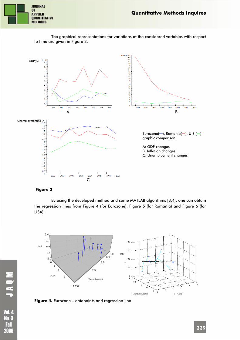
Quantitative Methods Inquires
339
The graphical representations for variations of the considered variables with respect to time are given in Figure 3.
A B
C
Figure 3
By using the developed method and some MATLAB algorithms [3,4], one can obtain
the regression lines from Figure 4 (for Eurozone), Figure 5 (for Romania) and Figure 6 (for USA).
Scatter Plot
C11
C9 C10
7.0
7.5
8.0
8.59.0
2.0
2.1
2.2
2.3
2.4
01
2
3
4
Figure 4. Eurozone – datapoints and regression line
GDP(%)
Unemployment(%)
Eurozone(▬), Romania(▬), U.S.(▬) graphic comparison: A: GDP changes B: Inflation changes C: Unemployment changes
Unemployment
GDP
Infl.
Infl.
GDP
Unemployment

Quantitative Methods Inquires
340
Scatter PlotC
3
C1 C2
6.0
6.5
7.07.5
8.08.5
0
10
20
30
40
50
24
6
8
10
Figure 5. Romania – datapoints and regression line
Scatter Plot
C7
C5 C6
3.0
3.54.0
4.55.0
5.56.0
1.01.5
2.0
2.5
3.0
3.5
01
2
3
4
Figure 6. United States–datapoints and regression line
4. Conclusions
A deterministic method for mapping the linear evolution of an economy using three main indicators, each of them regarded as a time function, was discussed. The algorithm was applied to a cross-national comparative study regarding economic changes in a period of several years.
References 1. Arthanary, T. S. and Dodge, Y. Mathematical programming in statistics, John Wiley and Sons,
New York, 1980 2. de Groen, P. An introduction to total least squares, Nieuw Archief voor Wiskunde, Vierde serie
14, 1996, pp. 237-253 3. Petras, I. and Podlubny, I. State space description of national economies: The V4 countries,
Computational Statistics & Data Analysis 52, 2007, pp. 1223-1233 4. Petras, I. and Podlubny, I. Orthogonal linear regression in 3D-space by using principal
components analysis. A function for MATLAB, MATLAB Central File Exchange, 2006
Unemployment
Unemployment
GDP
GDP
Infl.
Infl.
Unemployment
GDP
Infl.
Infl.
Unemployment
GDP

Quantitative Methods Inquires
341
Appendix In this section the following notations are used:
-The dot product (or the inner product) between three-dimensional vectors ( )321 ,, aaaa = and
( )321 ,, bbbb = is given by
332211 babababa ++=⋅
-The cross product is defined by
( )122131132332 ,, bababababababa −−−=×
Let ( )000 ,, zyxA be a point belonging to line l , ( ) kzjyixzyxr 0000000 ,, ++== (position
vector) and ( )cbav ,,= (direction vector). Consider an arbitrary point ( ) lzyxB ∈,, and
( )zyxr ,,= . Then there is a real number t such that vtAB = . Therefore one can write
=+= ABrr 0 vtr +0 (Fig. A). So the vector equation of the line is given by vtrr += 0 ,
R∈t (parameter). The vector equation is equivalent to ( ) ( ) ( )tctbtazyxzyx ,,,,,, 000 += , from
which the following parametric equations are derived: ctzzbtyyatxx +=+=+= 000 ,, , with
R∈t , or (if :)0,, ≠cba c
zzb
yya
xx 000 −=
−=
−.
Figure A Figure B
Consider ( )kkkk zyxP ,, a point in the three-dimensional space and the line l (defined as above). If
θ is the angle between kAP and v ( kPAQ ˆ=θ , Fig. B) it results the following relation between the
cross product and θsin :
θsin⋅⋅=× vAPvAP kk .
Thus, the formula for the distance from the point kP to the line l is given by:
v
vAP
vAP
vAPAPAPQPQP
k
k
kkkkk
×=
⋅
×⋅=== θsin .
Consequently,
( ) ( )=
++
×−−−=
222
000 ,,,,
cba
cbazzyyxxQP kkk
k
( ) ( ) ( ) ( ) ( ) ( )=
++
−−−−−−−−−=
222
000000 ,,
cba
ayybxxcxxazzbzzcyy kkkkkk
( ) ( )[ ] ( ) ( )[ ] ( ) ( )[ ]222
200
200
200
cbaayybxxcxxazzbzzcyy kkkkkk
++−−−+−−−+−−−
=

Quantitative Methods Inquires
342
The sum of squared distances from points ( ) mkzyxP kkkk ,1,,, = to l is:
( ) ( )[ ] ( ) ( )[ ] ( ) ( )[ ]{ }∑=
−−−+−−−+−−−++
m
kkkkkkk ayybxxcxxazzbzzcyy
cba 1
200
200
200222
1
If one set the first derivatives w.r.t. 000 ,, zyx equal to zero, obtain:
( ) ( )[ ] ( ) ( )[ ]{ } 01
0000 =−−−−−−−∑=
m
kkkkk ayybxxbcxxazzc
( ) ( )[ ] ( ) ( )[ ]{ } 01
0000 =−−−+−−−−∑=
m
kkkkk ayybxxabzzcyyc
( ) ( )[ ] ( ) ( )[ ]{ } 01
0000 =−−−−−−−∑=
m
kkkkk cxxazzabzzcyyb
which lead to
( ) ( )[ ] ( ) ( )[ ] 00000 =−−−−−−− ayybxxbcxxazzc
( ) ( )[ ] ( ) ( )[ ] 00000 =−−−+−−−− ayybxxabzzcyyc
( ) ( )[ ] ( ) ( )[ ] 00000 =−−−−−−− cxxazzabzzcyyb
or
( )( ) ( ) ( ) 00022
0 =−+−++−− aczzabyycbxx
( ) ( )( ) ( ) 0022
00 =−++−−− bczzcayyxxab
( ) ( ) ( )( ) 022000 =+−−−+− bazzbcyyacxx
Consider the determinant:
22
22
22
babcacbccaabacabcb
−−−−
−−=Δ
As (Column 1)= ⋅−ab
(Column 2)+ ⋅−ac
(Column 3) it result that 0=Δ .
Consider
( )222222
22
cbaccaab
abcb++=
−−−−
=Δ
( )( ) ( )( )0
22222
0
01 zzcbaac
cazzbcabzzac
−++=−−−−
−−=Δ
( )( ) ( )( )0
222
0
022
2 zzcbabczzbcabzzaccb
−++=−−−−−−
=Δ
Thus ( )01
0 zzcaxx −=
ΔΔ
=− and ( )02
0 zzcbyy −=
ΔΔ
=− . Hence c
zzb
yya
xx 000 −=
−=
−
and it’s obvious that the centroid belonging to the fitting line.
1Dr. Marius Giuclea graduated in Mathematics from University of Bucharest, Romania in 1994 and obtained his MSc degree in Mathematics in 1995. Between 1994 and 2001 he worked as scientific researcher at National Institute for Research and Development in Microtechnologies and from 2001 as lecturer at Academy of Economic Studies.

Quantitative Methods Inquires
343
In 2004 he was awarded a Ph.D. in applications of intelligent techniques in dynamic systems control by Institute of Mathematics, Bucharest. His research interests include intelligent techniques and their applications in modelling and control of dynamic systems. He is author of 3 books and about 35 publications in scientific journals and international conference proceedings. 2 Dr. Ciprian Popescu is author of 2 books and about 21 research papers in scientific journals, international and national conferences. 3Codification of references: [1] Arthanary, T. S. and Dodge, Y. Mathematical programming in statistics, John Wiley and Sons, New York,
1980 [2] de Groen, P. An introduction to total least squares, Nieuw Archief voor Wiskunde, Vierde serie 14, 1996,
pp. 237-253 [3] Petras, I. and Podlubny, I. State space description of national economies: The V4 countries,
Computational Statistics & Data Analysis 52, 2007, pp. 1223-1233 [4] Petras, I. and Podlubny, I. Orthogonal linear regression in 3D-space by using principal components
analysis. A function for MATLAB, MATLAB Central File Exchange, 2006

Quantitative Methods Inquires
344
A LOWER BOUND FOR PROJECT COMPLETION TIME ATTAINED BY DETAILING PROJECT TASKS AND
REDISTRIBUTING WORKLOADS
Zohar LASLO1 PhD, Associate Professor, Department of Industrial Engineering and Management, Sami Shamoon College of Engineering, P.O.Box 950, 84100, Beer-Sheva, Israel E-mail: [email protected]
Hagai ILANI2 PhD, Senior Lecturer, Department of Industrial Engineering and Management, Sami Shamoon College of Engineering, P.O.Box 950, 84100, Beer-Sheva, Israel E-mail: [email protected] Baruch KEREN3,4 PhD, Senior Lecturer, Department of Industrial Engineering and Management, Sami Shamoon College of Engineering, P.O.Box 950, 84100, Beer-Sheva, Israel E-mail: [email protected]
Abstract: We evaluate the possible benefit from improving the workload distribution in a directed acyclic graph (DAG) (e.g. a project network), by determining a lower bound for the project completion time. It is shown that a lower bound can be obtained by equally distributing the workload over the max-cut in the graph which separates the nodes 1 and n. It is also shown that for a complete n-node DAG, practitioners can quickly compute a lower bound for the project completion time. The max-cut can be found by any linear programming algorithm or by reducing the problem to the problem of finding a maximum matching in a bipartite graph. Our results can help planners and project managers to characterize the "ideal case" in which the optimal workload distribution among the arc networks minimizes the project completion time. That can be done for a non-complete DAG as well as for a complete one. A lower bound can then be used to evaluate the maximum potential for reducing the project completion time in real-life cases. Key words: Project network; Directed acyclic graph (DAG); Max-cut; Maximum matching, Bipartite graph

Quantitative Methods Inquires
345
1. Introduction
A reduction in project completion time is one of the main missions in project management and in similar processing contexts. We evaluate the possible benefit from improving the workload distribution in a directed acyclic graph (DAG) (e.g. a project network), by determining a lower bound for the project completion time. Revealing the lower bound of a project's completion time is critical for managers, as the lower bound gives significant information about the potential value for investing effort and management time for reducing the project completion time. If the planned processing time of a given plan/project is near the lower bound, the mangers can deduce that the potential reduction is small (large), and by that decide if it is worthwhile to spend effort and time in trying to accelerate the project.
The objective of shortening the project completion time can be attained by additional budget and/or by redistribution of workloads, the latter being more economical but less feasible. The current common methodologies for shortening the project completion time are based on investment of additional budget in the critical path activities in deterministic models [1-2]5 or in the high criticality activities in stochastic models [3-6]. The procedures for optimal redistribution of budget among project activities ([1- 6]) enable the minimizing of the project completion time under budget constraints. The precedence among the project activities as well as the activities "crash" durations determine a lower bound for the project completion time. It is obvious that releasing the budget constraints by bringing all the activity execution times to “crash” paces, i.e., maximal execution speed can reveal the lower bound of the project completion time that can attained by additional budget.
The problem of scheduling directed acyclic task flow graphs has been examined in many forms in information technology for multiprocessor systems. Hary and Oezguener [7] studied the problem of scheduling directed acyclic task flow graphs to multiprocessor systems using point-to-point networks. Ahmad et al. [8] surveyed 21 algorithms that allocate a parallel program represented by an edge-weighted directed acyclic graph to a set of homogeneous processors, with the objective of minimizing the completion time.
Luh and Lin [9] claimed that it is possible to achieve minimum production time and increased productivity through the use of parallel operations in parts fabrication as well as in assembly, computation and control of industrial robots. However, the coupling between consecutive phases of the operations which results in series-parallel precedence constraints may, in turn, create unavoidable idle time intervals during the operations. Luh and Lin developed an algorithm that determines a minimum time-ordered schedule for the parallel operations. Their algorithm was based on the Program Evaluation and Review Technique (PERT).
For over three decades now researchers have sought effective solution procedures for shortening the critical paths in PERT types scheduling problems under conditions of limited resources availability [10]. Phillips [11] presented a procedure for these problems with multiple parallel processors that locates and verifies an optimal schedule for a project, under conditions of multiple resource constraints. The procedure is network-based and uses a graphical cut-search-approach. The optimal solution can be obtained iteratively by constructing a minimum cost network flow problem and adjusting the durations of activities corresponding to a minimum capacity cut-set. Baker [12] showed that the same can be done simply by using linear programming formulation.

Quantitative Methods Inquires
346
A shorter project completion time can be attained by subdividing the work breakdown structure (WBS), and/or by redistributing the workload among activities, if possible and feasible. Laslo et al. [13] introduced a linear programming optimization that can be implemented for redistributing removable workload fragments among project activities for minimizing the project completion time. This was done without violating the precedence relations within the project.
One of the key features of project planning is the utilization of a WBS to show the hierarchy of tasks within a project and to define work packages [14]. The detailing of project tasks into sub-tasks can be done down to lower levels until reaching the level where the sub-tasks finally become manageable units (so-called work packages) for planning and control [15]. Detailing of project tasks and precedence relationships is theoretically an economic option for shortening the project completion time. The detailing of project tasks is unlimited, but one must take into consideration the manageability of the project, i.e., the DAG size that has to be determined by the number of arcs and by the number of nodes. Over-detailing
increases the nodes and the arcs of the DAG up to n2⎛ ⎞⎟⎜ ⎟⎜ ⎟⎜ ⎟⎜⎝ ⎠
arcs in a complete n-node DAG.
However, [16] proved that random acyclic digraphs have only n2/4 arcs on average. The lower bound of the n-node DAG completion time is determined by taking into
account the "ideal case" in which the optimal workload distribution among the given arc networks minimizes the project completion time. One important objective of this paper is to characterize the properties of this "ideal case". An additional objective is to show how to find for a pre-given total workload and a pre-given DAG this "ideal case", i.e. to compute a lower bound of the project completion time. To solve the problem of determining the optimal workload distribution, we use a special form of the max-flow problem, a special form of the maximum matching problem and Dilworth’s Theorem [17].
The paper proceeds as follows: Section 2 defines the problem; Section 3 presents the linear programming solution for workload distribution; Section 4 presents a solution for the same problem by combinatorial optimization; Section 5 presents an algorithm for finding a max-cut of a DAG; Section 6 suggests a closed-form formula to compute the size of the max-cut of a complete DAG; and Section 7 concludes the paper. The main contributions of this paper for practitioners are that we propose a simple algorithm to find a max-cut in a DAG which is needed for lower bound computation and a closed-form formula to compute the size of the max-cut of a complete DAG.
2. Problem definition
Let us consider an activity-on-arc directed acyclic graph G( N ,A ) where N is a
set of n nodes, topologically sorted, and A is a set of m arcs denoted by i , jA . Each of the
m arcs has one unit of processing capacity, in which case we can consider the arc workload
as the processing time of this arc. The graph G( N ,A ) has one source node 1N and one
sink node nN . The i , jA 's arc workload i , jt is a non-negative variable. All the series paths in
the graph, denoted by pP and with length pT , start at the source node 1N and end at the

Quantitative Methods Inquires
347
sink node nN . Let us also consider unlimited options for distributing the spread-out
cumulative total workload T among the arcs i , jA , i.e., the workload distribution is subject
to
i , j
i , jA A
T t∈
= ∑ .
The task execution time of a DAG is equivalent to the length of the longest path,
i.e., the critical path, c pT max(T )= . The most favorable planning for a given DAG is that
in which the cumulative spread-out workload T is distributed such that it minimizes the critical path. The solution for the most favorable planning of workload distribution problem
denoted, by MP( G,T ) , is any feasible solution i , ji , j A A{ t }τ ∈= that minimizes the
objective function c pT max(T )= subject to
i , j
i , jA A
T t∈
= ∑ . Thus, the solution of the
MP( G,T ) problem is equivalent to finding a lower bound for the project completion time.
For the remainder of the paper we use the following notation:
A - a set of m arcs.
i , jA - an arc (arrow), i , jA A∈ .
Di, jA - a dummy arc with i , jt 0= , D
i, jA A∈ .
Ei, jA - an effective arc with i , jt 0> , E
i, jA A∈ .
G( N ,A ) - an activity-on-arc directed acyclic graph.
m - the number of arcs i , jA A∈ .
N - a set of n nodes, topologically sorted.
kN - the k -th node, kN N∈ 1 k n≤ ≤ . n - the number of nodes kN N∈ .
pP - the p -th path starting at the source node 1N and ending at the sink node
nN . q - the number of paths. r - the minimal number of paths that covers the m network arcs i , jA A∈ .
sτ - the number of effective arcs Ei, jA A∈ in a feasible solution τ .
T - the cumulative total spread-out workload
i , j
i , jA A
T t∈
= ∑ .
cT - the task execution time, which is the joint workload of the critical path, c pT max(T )= .
pT - the joint-workload on pP , p
i , j
pi , j
A PT t
∈
= ∑ .
i , jt - the i , jA 's workload (variable), i , jt 0≥ . Since each i , jA has one unit of
processing capacity i , jt can be considered as the processing time.

Quantitative Methods Inquires
348
τ - a feasible distribution, i , ji , j A A{ t }τ ∈= .
( , )X X - a cut-set of arcs induced by a set X of nodes that includes 1N ,and its
complement X that includes nN ; each arc jiA , in the cut-set has its tail in
X and its head in X .
π - a set of paths pP that covers all the arcs i , jA A∈ .
3. The linear programming solution for the workload distribution problem
The MP( G,T ) problem can be set as a special case of a flow linear programming
problem for any n -node graph. Let iT be the time of completing all the activities ending at
node i . Then the linear programming formulation for the problem is:
nMin T
s.t.
1 0T =
, , ,2,..., ; 1, 2,...,1; { }j i i j i j A Ai j
T T t j n i j j t ∈− ≥ = = − −
,{ }, ,
i jti j A Ai j
t T∈
=∑
0 1,...,iT i n≥ =
Now let us consider an example of a DAG with n 5= , m 8= and, q 5= as
presented in Figure 1.
Figure 1. Directed acyclic graph
A1,2
A1,4
A1,5
A2,3
A2,4
A2,5 A3,5
A3,4
A3,5
max-cut
1
2
4
3
5

Quantitative Methods Inquires
349
The linear programming formulation for this example is:
5Min T
s.t.
1 0T =
2 1 1,2 0T T t− − ≥
4 1 1,4 0T T t− − ≥
5 1 1,5 0T T t− − ≥
3 2 2,3 0T T t− − ≥
4 2 2,4 0T T t− − ≥
5 2 2,5 0T T t− − ≥
5 3 3,5 0T T t− − ≥
5 4 4,5 0T T t− − ≥
1,2 1,4 1,5 2,3 2,4 2,5 3,5 4,5t t t t t t t t T+ + + + + + + =
, ,0i j i jt A A≥ ∀ ∈ .
The two optimal basic solutions for this example are presented in Table 1. Table 1. The optimal workload assignment for minimizing the execution time
Variable Optimum I Optimum II t1,2 0 0 t1,4 0.2T 0.2T t1,5 0.2T 0.2T t2,3 0.2T 0 t2,4 0.2T 0.2T t2,5 0.2T 0.2T t3,5 0 0.2T t4,5 0 0 Tc 0.2T 0.2T
Linear programming is an easy way to solve small MP( G,T ) problems, but it has
disadvantages. The first disadvantage is that it needs many variables and many constraints
that must be compiled and satisfied. The linear programming formulation for n-node DAG
has up to n
12⎛ ⎞⎟⎜ ⎟+⎜ ⎟⎜ ⎟⎜⎝ ⎠
constraints, n
m2⎛ ⎞⎟⎜ ⎟=⎜ ⎟⎜ ⎟⎜⎝ ⎠
viable arrows and n 2q 2 −= paths. The second
disadvantage is that with linear programming it is more difficult to explore solution
properties. Therefore, in the following sections we present a procedure to solve MP( G,T )
problems by combinatorial optimization

Quantitative Methods Inquires
350
4. A solution for the workload distribution problem by combinatorial optimization
Now we use a combinatorial optimization to derive a solution for the n -node
graph workload distribution problem MP( G,T ) . As the following theorems show, some
interesting results can be obtained by combinatorial optimization. Theorem 1 states that an optimal distribution of the cumulative spread-out
workload T is obtained by uniform distribution of T over the arcs of some maximum
directed cut which separates nodes 1N and nN . We define a directed cut as the set of arcs
formed by a partition of the node-set N to two parts X , X so that 1 , nN X N X∈ ∈ and
the set of arcs directed from X to X is empty. The arcs which belong to a cut are those
which are directed from X to X . Such a cut is denoted as ( )X ,X . The size of the cut is
denoted by ( , )X X .
Theorem 1. cmin(T ) with the cumulative spread-out workload T equals
{ }T max ( X ,X ) , where the maximum is over all the directed cuts ( , )X X that separate
the nodes 1N and nN . (The proof of Theorem 1 can be found in the Appendix. This proof
used Lemma 1 and Dilworth's Theorem which also in the Appendix.)
Theorem 2. An arc is an effective arc Ei, jA in some feasible solution τ if it belongs to some
max directed cut which separates nodes 1N and nN . (For the proof see the Appendix.)
It follows from Theorem 2 that sτ , the number of effective arcs Ei, jA in a given
feasible solution τ , is at least the size of a max directed cut which separates nodes 1N and
nN : s rτ ≥
By a reduction to Dilworth's Theorem, as done in the proof for Theorem 1, we get the following corollary:
Corollary 1. The problem MP( G,T ) is polynomially solvable by standard min-flow-max-
cut algorithms that solve Dilworth's problem.
5. An algorithm for finding a max-cut of a DAG
The proposed algorithm for finding a max-cut of a DAG is based on the concept of maximum matching (see [18], Section 26.3). The basic idea is to present the DAG by a bipartite graph and then to apply an algorithm for finding a maximum matching.
Before describing and applying the algorithm, we need to recall some notions from matching theory. A matching M in a graph is a set of edges of which any two do not have a common end. Given a matching M in a graph, an alternating path with respect to M is a path whose edges alternate between matched edges and non-matched edges. An isolated vertex will also be considered as an alternating path although it is not an end of any edge. A vertex is called M-exposed if it is not an end of a matched edge.

Quantitative Methods Inquires
351
The algorithm proceeds as follows: Step 1: Construct a bipartite graph H associated with the DAG. The vertex set of H is then
constructed as follows. For any arc jiA , we introduce two vertices: a start vertex
SjiA )( , and a finish vertex F
jiA )( , . Let S denote the set of start vertices and F denote
the set of finish vertices. S and F partition the vertex set of the bipartite graph H into
its two parts. The edge set of H consists of pairs of vertices ( SjiA )( , , F
lkA )( , ) where the
two arcs jiA , and lkA , belong to some directed path in the DAG starting at jiA , and
ending at lkA , . An illustration of the bipartite graph H associated with the DAG in
Figure 1 is given in Figure 2. The bold edges form a maximum matching in H.
Figure 2. Description of the directed acyclic graph (Figure 1) by a bipartite graph Step 2: Find a maximum matching M in H. Efficient algorithms for finding a maximum
matching can be found in any combinatorial optimization book, e.g. [18]. Step 3: Scan the graph H in order to find all the vertices which belong to some alternating
path starting at an M-exposed vertex of S. A vertex found by the scanning will be called a scanned vertex. This scanning is actually what is done before termination of any algorithm for finding a maximum matching, see [18].
Step 4:
Look for the arcs jiA , of the DAG which were scanned exactly once at H (either the
start vertex SjiA )( , was scanned, or the finish vertex F
jiA )( , was scanned, but not
both nor none of them) in Step 3. These arcs are the arcs of a max-cut in the DAG, see [19].
(A1,5)F
(A2,3)F
(A2,4)F
(A2,5)F
(A3,5)F
(A4,5)F
(A1,2)F
(A1,4)F
(A1,5)S
(A2,3)S
(A2,4)S
(A2,5)S
(A3,5)S
(A4,5)S
(A1,2)S
(A1,4)S
edges edges of the matching M

Quantitative Methods Inquires
352
Figure 3. Alternating paths and scanned vertices Figure 3 illustrates the alternating paths and the scanned vertices of the DAG that
presented are in Figures 1 and 2. The alternating paths (see Figure 3) starting at M-exposed
vertices of S are the isolated vertices of S, SSSS AAAA )(,)(,)(,)( 5,45,35,25,1 and the path
))(,)(,)(( 4,25,44,1SFS AAA . Therefore, the scanned vertices are
SFSSSSS AAAAAAA )(,)(,)(,)(,)(,)(,)( 4,25,44,15,45,35,25,1 . The arcs of the DAG of which exactly
one of their start vertexes and finish vertexes is scanned (Step 4) are
4,25,35,25,14,1 ,,,, AAAAA . These are the arcs of a max-cut (see Figure 1).
6. The size of the max-cut of a complete DAG
It is obvious that n-node DAG with the maximal number of viable arrows
n2⎛ ⎞⎟⎜ ⎟⎜ ⎟⎜ ⎟⎜⎝ ⎠
enables us to attain a better solution to the MP( G,T ) problem, or at least one that is
no worse than the solution for an n-node DAG with n
m2⎛ ⎞⎟⎜ ⎟<⎜ ⎟⎜ ⎟⎜⎝ ⎠
arcs. This is because each
additional arc i , jA can be loaded or remain unloaded. From Theorem 1 we get an
additional corollary that enables us to easily calculate the size of a max-cut of a complete
DAG, and from this to compute a lower bound for cT .
Corollary 2. If ( , )G N A is the complete graph with n nodes and n2⎛ ⎞⎟⎜ ⎟⎜ ⎟⎜ ⎟⎜⎝ ⎠
arcs, then the size of
the max-cut is: { } 2nmax |( X , X )| 4⎢ ⎥
= ⎢ ⎥⎢ ⎥⎣ ⎦
,
and as consequence, the cT of an optimal distribution τ of T for MP( G,T ) is:
(A4,5)S
(A3,5)S
(A2,5)S
(A2,4)S
(A1,5)S
(A1,4)S
(A2,3)S
(A1,2)S
(A1,5)F
(A2,3)F
(A2,4)F
(A2,5)F
(A3,5)F
(A4,5)F
(A1,2)F
(A1,4)F

Quantitative Methods Inquires
353
c2Tmin(T )
n4
=⎢ ⎥⎢ ⎥⎢ ⎥⎣ ⎦
. (For the proof see the Appendix.)
7. Summary and conclusions
The aim of this paper was to evaluate the possible benefits from improving the workload distribution in a DAG (e.g. a project network), by determining a lower bound of the project completion time. We proved that a lower bound can be obtained by dividing the total cumulative processing time uniformly among the arcs on a max-cut set. That is the maximum parallel planning for a given DAG. We also presented a combinatorial algorithm for finding the max-cut, based on a maximum matching algorithm. The simple closed-form solution for
the complete n-node DAG case 2 4n⎢ ⎥⎣ ⎦ can be a very useful formula to calculate a lower
bound of the completion time of any DAG.
The value of the term ( )2/ 4 / ( , )T n T X X⎢ ⎥ −⎣ ⎦ can be an indication of the
benefit derived from further detailing of the project tasks and from increasing edges up to a
complete graph. This is because the difference between 2 4n⎢ ⎥⎣ ⎦ , the max-cut size of a
complete DAG, and ( , )X X , the max-cut size of any DAG, represents further potential for
shortening the project completion time that can attained by more detailing of project tasks. The results in this paper can help planners and project managers to characterize
the "ideal case" in which the optimal workload distribution among the arc networks minimizes the project completion time. That can be done for a non-complete DAG as well as for a complete one. A lower bound can then be used to evaluate the maximum potential for reducing the project completion time in real-life cases.
References 1. Ahmad, I., Kwok, Y.-K. and Wu, M.-Y. Analysis, evaluation and comparison of algorithms for
scheduling task graphs on parallel processors, “Proceedings of the International Symposium on Parallel Architectures, Algorithms and Networks”, Beijing, China, 1996, pp.207-213
2. Baker, B.M. Cost time trade-off analysis for the critical path method: a derivation of the network flow approach, Journal of the Operations Research Society, vol. 48, 1997, pp. 1241-1244
3. Brightwell, G. Partial orders, in graph connections, (Beineke, L.W. and Wilson, R.J. Eds.) Oxford University Press, 1997, pp.52–69
4. Cook, W.J., Cunningham, W.H., Pulleyblank, W.R. and Schrijver, A. Combinatorial Optimization, John Wiley & Sons, INC., New York, 1998, pp. 53-62
5. Cormen, T.H., Leiserson, C.E., Rivest, R.L.and Stein, C. Introduction to Algorithms, Second Edition, The MIT Press and McGraw-Hill, 2001
6. Golenko-Ginzburg, D. and Gonik, A. A heuristic for network project scheduling with random activity durations depending on the resource reallocation, International Journal of Production Economics, vol. 55(2), 1998, pp. 149-162

Quantitative Methods Inquires
354
7. Golenko-Ginzburg, D., Gonik, A. and Kesler, S. Hierarchical decision-making model for planning and controlling stochastic projects, International Journal of Production Economics, vol. 46/47, 1996, pp. 39-54
8. Golenko-Ginzburg, D., Gonik, A. and Sitniakovski, S. Resource supportability model for stochastic network projects under a chance constraint, Communications in Dependability and Quality Management, vol. 3(1), 2000, pp. 89-102
9. Hary, S.L. and Oezguener, F. Precedence-constrained task allocation onto point-to-point networks for pipelined execution, IEEE Transactions on Parallel and Distributed Systems, vol. 10(8), 1999, pp. 838-851
10. Kelley, J.E. and Walker, M.R. Critical path planning and scheduling, in “Proc. of the Eastern Joint Computer Conference”, 1959, pp. 160-173
11. Kelley, J.E. Critical path planning and scheduling: mathematical basis, Operations Research, vol. 9(3), 1961, pp. 296-320
12. Laslo, Z. Activity time-cost tradeoffs under time and cost chance constraints, Computers & Industrial Engineering, vol. 44(3), 2003, pp. 365-384
13. Laslo, Z., Keren, B. and Ilani, H. Minimizing task completion time with the execution set method, European Journal of Operational Research, 187, 2008, pp. 1513–1519
14. Lavold, G. Developing and using the work breakdown structure, in Clealand, D. and King, W. (Eds.), “Project Management Handbook”, Van-Nostrand Reinhold Company Inc., New York, 1988
15. Luh, J.Y.C. and Lin, C.S. Scheduling parallel operations in automation for minimum execution time based on PERT, Computers & Industrial Engineering, vol. 9(2), 1985, pp.149-165
16. Melançon, G., Dutour, I.and Bousquet-Mélou, M. Random generation of directed acyclic graphs, in Nesetril, J., Noy, M. and Serra, O. (Eds.), Comb01, “Euroconference on Combinatorics, Graph Theory and Applications, in: Electronic Notes in Discrete Mathematics”, vol. 10, 2001
17. Phillips, S. Jr. Project management duration/resource tradeoff analysis: an application of the cut search approach, Journal of the Operations Research Society, vol. 47, 1996, pp. 697-701
18. Simpson, W.P. III and Patterson, J.H. A Multiple-tree search procedure for the resource-constrained project scheduling problem, European Journal of Operational Research, vol. 89(3), 1996, pp. 525-542
19. * * * DOD and NASA Guide, PERT Cost Systems Design, by the Office of the Secretary of Defense and National Aeronautics and Space Administration, U.S. Government Printing Office, Washington, D.C., June 1962
Appendix
Lemma 1. If 1 r{ P ,...,P }π= , 1 r q≤ ≤ is a cover of the arcs i , jA by paths pP ,
1 p r≤ ≤ and τ is a feasible solution, then
(1) c TTr
≥ .
Moreover, if equality holds, then all paths in π are of joint-workload pT T r= and each
arc i , jA which is covered more than once by π has workload i , jt 0= , i.e. it is a dummy or
unnecessary arc Di, jA .

Quantitative Methods Inquires
355
Proof of Lemma 1. Let π be a cover of the arcs i , jA by paths pP , 1 p r≤ ≤ , and let τ
be a feasible solution. Since τ is a feasible solution, it satisfies the constraint
i , j
i , jA A
T t∈
= ∑ .
π is a cover of the arcs and hence, (2)
pi , ji , j
r rp
i, j i , jp 1 p 1 A AA P
T t t T= = ∈∈
= ≥ =∑ ∑ ∑ ∑ ,
It follows that there must be a path pP in π satisfying, p
i , j
i , jA P
t T r∈
≥∑ and therefore
cT T r≥ . From (2) it follows that equality holds if all paths in π have the same workload
pT and each arc i , jA , which is covered more than once by π , has workload i , jt 0= , i.e.
each such arc should be classified as Di, jA .
The following theorem is a version of Dilworth's Theorem [4].
Dilworth's Theorem. Let ( , )G N A be an acyclic network where the nodes 1 nN ,... ...,N
are topologically sorted and let d be a non-negative integral function on the arc set A .
Then, the minimum number of pP s which cover each arc i , jA at least ,( )i jd A times equals
i , j
i , jA ( X ,X )
max d( A )∈∑ where the maximum is over the cuts ( X ,X ) that separate the
nodes 1N and nN , i.e.
i ,i
i , jA ( X ,X )
max d( A )|1 X ,n X∈
⎧ ⎫⎪ ⎪⎪ ⎪⎪ ⎪∈ ∈⎨ ⎬⎪ ⎪⎪ ⎪⎪ ⎪⎩ ⎭∑ .
Proof of Theorem 1. Let ( , )X X be a cut separating nodes 1N and nN of cardinality r .
Also, let ( X ,X )τ be the distribution of the cumulative spread-out workload T obtained by
distributing T uniformly on the edges of the cut ( , )X X . Since every pP contains a single
arc of the cut ( , )X X the following inequality is valid:
(3) c c( X ,X )
Tmin T ( ) Tr
τ τ≤ = .
for any feasible solution τ . Since the above is true for any cut, it is also true for a cut with maximum cardinality and hence,
(4)
{ }c Tmin T ( )
max |( X ,X )|τ ≤ .
On the other hand, let ( , )X X be a cut that separates nodes 1N and nN of maximum
cardinality and τ be a distribution of the cumulative spread-out workload T that minimizes
the left-hand side of (4). By taking 1d ≡ in Dilworth's Theorem we get that the cardinality of

Quantitative Methods Inquires
356
the cut ( , )X X is equal to some covering π of the arc set A by paths pP . It follows from
Lemma 1 that { }cT ( ) T max |( X , X )|τ ≥ . This completes the theorem's proof.
Proof of Theorem 2. Let i , jA be an arbitrary arc. If i , jA belongs to some max-cut which
separates nodes 1N and nN , then the optimum solution ( X ,X )τ assigns the workload
i , jt T ( X ,X )= to i , jA and therefore it is an effective arc Ei, jA . Conversely, suppose i , jA
doesn't belong to any max-cut which separates nodes 1N and nN . We again apply
Dilworth's Theorem with d equaling 1 everywhere except at the arc i , jA where it equals 2.
Since i , jA doesn't belong to any max-cut which separates nodes 1N and nN , it follows that
any max-cut which separates nodes 1N and nN maximizes the objective function
i , j
i , jA ( X ,X )
d( A )∈∑ . Therefore, by the theorem there is a cover π of the arcs by paths pP
that covers the arc i , jA twice and has the cardinality of a max-cut. Thus by the last claim of
Lemma 1, in any distribution τ of T for which inequality (1) holds with equality the arc i , jA
is assigned i , jt 0= . But for cover π , which has the cardinality of a max-cut, a distribution
τ of T fulfills equality in (1) if it is an optimum solution. Therefore, i , jA is a dummy or
unnecessary arc Di, jA .
Proof of Corollary 2. By Theorem 1, the cT ( )τ for an optimal distribution τ of T equals
T divided by the size of a max-cut which separates nodes 1N and nN . When the given
network is a complete network, the cut that separates nodes 1N and nN is the set of arcs
connecting the first r nodes 1 rN ,... ...,N with the last n r− nodes r 1 nN ,... ...,N+ for some
r (1 r n 1≤ ≤ − ). By straightforward calculus, the max-cut separates the first n 2 nodes
( n 2⎢ ⎥⎣ ⎦ or n 2⎡ ⎤⎢ ⎥ when n is odd) from the last n 2 nodes ( n 2⎡ ⎤⎢ ⎥ or n 2⎢ ⎥⎣ ⎦ when n is odd)
and is of size 2n 4⎢ ⎥⎢ ⎥⎣ ⎦
.
1Zohar Laslo is Associate Professor and Dean of the Industrial Engineering and Management, SCE - Shamoon College of Engineering, Israel. Zohar was born in 1945. He received his B.Sc. and M.Sc. in Industrial Engineering and Management from the Technion - Israel Institute of Technology, Haifa, and his Ph.D. degree in Industrial Engineering and Management (Summa Cum Laude) from the Ben Gurion University of the Negev, Israel. His professional experience includes 24 years of engineering and management positions in Israeli aeronautical, electro-optical, pharmaceutical industries. His current research interests are in matrix structure performance, network design, planning scheduling and control, planning under time-cost uncertainty, quality of planning, maintainability and hazard analysis techniques, and technological education. His recent publications have appeared in International Journal of Project Management, International Journal of Production Economics, Journal of Applied Quantitative Methods, European Journal of Operational Research, Computer Modelling and New Technologies, Journal of Business Economics and Management, Technological and Economic Development of Economy, Transport and Telecommunication, Communications in Dependability and Quality Management, Computers & Industrial

Quantitative Methods Inquires
357
Engineering, Mathematics and Computers in Simulation, Automation and Remote Control, OMO the Journal of Terotechnology, IEEE Transactions on Engineering Management, Tribology in industry and European Journal of Engineering Education. 2 Hagai Ilani is Senior Lecturer and Head Head of the Industrial Engineering and Industrial Management department in Ashdod Campus, SCE - Shamoon College of Engineering, Israel. Hagai was born in 1966. He received his B.Sc., M.Sc, and Ph.D. in Mathematics from the Ben Gurion University of the Negev. His current research interests are in combinatorial optimization and meta-heuristics algorithms for NP-hard optimization problems. His recent publications have appeared in European Journal of Operational Research and Journal of Combinatorial Theory. 3 Corresponding author: Tel: +972-8-647-5641/42/48 Fax: +972-8-647-5643 E-Mail: [email protected] 4 Baruch Keren is a Senior Lecturer and Head of the Industrial Systems Track in the Industrial Engineering and Management Department, SCE - Shamoon College of Engineering, Israel, and lecturer at the Open University of Israel. Baruch was born in 1958. He received his B.Sc., M.Sc. and Ph.D. (Summa Cum Laude) in industrial engineering from Ben-Gurion University. His professional experience includes 13 years of several professional positions in the Israel Chemicals Ltd. and its subsidiaries in the areas of industrial engineering, economics and auditing.His current research interests are in decision-making under uncertainty, production planning, project management and operations research. His recent publications have appeared in International Journal of Production Economics, Omega, European Journal of Operational Research and IEEE Transactions on Reliability. 5 Codification of references:
[1] Kelley, J.E. and Walker, M.R. Critical path planning and scheduling, in “Proc. of the Eastern Joint Computer Conference”, 1959, pp. 160-173
[2] Kelley, J.E. Critical path planning and scheduling: mathematical basis, Operations Research, vol. 9(3), 1961, pp. 296-320
[3] Laslo, Z. Activity time-cost tradeoffs under time and cost chance constraints, Computers & Industrial Engineering, vol. 44(3), 2003, pp. 365-384
[4] Golenko-Ginzburg, D., Gonik, A. and Kesler, S. Hierarchical decision-making model for planning and controlling stochastic projects, International Journal of Production Economics, vol. 46/47, 1996, pp. 39-54
[5] Golenko-Ginzburg, D. and Gonik, A. A heuristic for network project scheduling with random activity durations depending on the resource reallocation, International Journal of Production Economics, vol. 55(2), 1998, pp. 149-162
[6] Golenko-Ginzburg, D., Gonik, A. and Sitniakovski, S. Resource supportability model for stochastic network projects under a chance constraint, Communications in Dependability and Quality Management, vol. 3(1), 2000, pp. 89-102
[7] Hary, S.L. and Oezguener, F. Precedence-constrained task allocation onto point-to-point networks for pipelined execution, IEEE Transactions on Parallel and Distributed Systems, vol. 10(8), 1999, pp. 838-851
[8] Ahmad, I., Kwok, Y.-K. and Wu, M.-Y. Analysis, evaluation and comparison of algorithms for scheduling task graphs on parallel processors, “Proceedings of the International Symposium on Parallel Architectures, Algorithms and Networks”, Beijing, China, 1996, pp.207-213
[9] Luh, J.Y.C. and Lin, C.S. Scheduling parallel operations in automation for minimum execution time based on PERT, Computers & Industrial Engineering, vol. 9(2), 1985, pp.149-165
[10] Simpson, W.P. III and Patterson, J.H. A Multiple-tree search procedure for the resource-constrained project scheduling problem, European Journal of Operational Research, vol. 89(3), 1996, pp. 525-542
[11] Phillips, S. Jr. Project management duration/resource tradeoff analysis: an application of the cut search approach, Journal of the Operations Research Society, vol. 47, 1996, pp. 697-701
[12] Baker, B.M. Cost time trade-off analysis for the critical path method: a derivation of the network flow approach, Journal of the Operations Research Society, vol. 48, 1997, pp. 1241-1244
[13] Laslo, Z., Keren, B. and Ilani, H. Minimizing task completion time with the execution set method, European Journal of Operational Research, 187, 2008, pp. 1513–1519
[14] * * * DOD and NASA Guide, PERT Cost Systems Design, by the Office of the Secretary of Defense and National Aeronautics and Space Administration, U.S. Government Printing Office, Washington, D.C., June 1962

Quantitative Methods Inquires
358
[15] Lavold, G. Developing and using the work breakdown structure, in Clealand, D. and King, W.
(Eds.), “Project Management Handbook”, Van-Nostrand Reinhold Company Inc., New York, 1988
[16] Melançon, G., Dutour, I.and Bousquet-Mélou, M. Random generation of directed acyclic graphs, in Nesetril, J., Noy, M. and Serra, O. (Eds.), Comb01, “Euroconference on Combinatorics, Graph Theory and Applications, in: Electronic Notes in Discrete Mathematics”, vol. 10, 2001
[17] Cook, W.J., Cunningham, W.H., Pulleyblank, W.R. and Schrijver, A. Combinatorial Optimization, John Wiley & Sons, INC., New York, 1998, pp. 53-62
[18] Cormen, T.H., Leiserson, C.E., Rivest, R.L.and Stein, C. Introduction to Algorithms, Second Edition, The MIT Press and McGraw-Hill, 2001
[19] Brightwell, G. Partial orders, in graph connections, (Beineke, L.W. and Wilson, R.J. Eds.) Oxford University Press, 1997, pp.52–69

Software Analysis
359
STAGES FOR THE DEVELOPMENT OF THE AUDIT PROCESSES OF DISTRIBUTED INFORMATICS SYSTEMS1
Marius POPA2 PhD, University Lecturer, Department of Computer Science in Economics, University of Economics, Bucharest, Romania E-mail: [email protected]
Cristian TOMA3 PhD, University Lecturer, Department of Computer Science in Economics, University of Economics, Bucharest, Romania E-mail: [email protected]
Abstract: The paper presents elements regarding the way in which an audit process is carried out. The following issues are highlighted: audit concept, audit process flow, audit program and audit program management, classes of audit processes, audit process stages and activities, documents used to conclude an audit process. In this paper, the audit concept is defined together with its characteristics and it is described as activities flow in which there are some stages and steps that must be passed in an audit process. The audit program term is presented together with stages followed in such program management. The paper contains classifications of the audit processes depending on many criteria and it offers some details about the audit process classes. The audit process must be rigorously carried out in accordance to stages established by audit specialists and included in standardized documents. During the audit process, the audit team members generate and fill in some documents and forms to support the audit report. The conclusions included in the audit report are based on audit evidences and observations obtained in audit process. Key words: Audit process; audit stages; distributed informatics system
1. Characteristics of the informatics audit processes In accordance with (ISO 19011, 2003), the concept of audit means a systematic,
independent and documented process to obtain audit evidences and their examination with impartiality to establish the degree in which the audit criteria are met. The examination is

Software Analysis
360
made by persons having specific qualifications who are independent in relation to audit process.
The audit evidences are represented by records, declarations about facts or other information relevant in relation to audit criteria. They are evaluated quantitatively or qualitatively.
The audit criteria represent a set of policies, procedures and requirements. One or more audit processes compose an audit program. The audits included in an
audit program are planned during period of time and they are oriented to a specific purpose. The process flow for management of an audit program is depicted in figure 1 (ISO 19011, 2003).
Figure 1. Process flow for audit program management
An audit program contains activities which:
• Plan and organize different audit processes as types and numbers;
• Supply resources for efficacy and efficient execution of the audits in planned
interval.
The stage for establishing the audit program includes activities regarding the
following issues:
• Purposes and scope – anticipated outcome and amplitude of the audit program
are determined by size, type and complexity of the audited organization;
• Responsibilities – they are assigned to persons who understand the audit
principles, auditors’ competencies and applying the audit techniques; these
persons must have management skills and understanding of the technical issues
in a business;
• Resources – they are the support of the audit program and there are financial,
economic and time ones;
• Procedures – they specify operations arranged in a step-by-step method followed
to reach the purpose.
The stage for audit program implementation contains the following activities:
• Audit programming – it refers to the activities regarding the coordination and
programming of the audits;

Software Analysis
361
• Auditors’ evaluation – it aims the permanent professional improvement and
auditors’ evaluation;
• Audit team selection – persons with professional skills in audit process are
included in audit team;
• Audit activity management – it refers to all activities regarding the audit carrying
out;
• Records maintenance – it is useful to demonstrate the audit program
implementation and the following records are included: records for each audit,
results of the audit program analysis and records regarding personnel used in
audit process.
The stage for monitoring and analyzing the audit program contains activities
regarding:
• Monitoring and analysis – accomplishment of the objectives is assessed at some
intervals; also, some performance indicators are used to determined the
accomplishment degree;
• Identifying the need for corrective and preventive actions – it results from
monitoring and analysis;
• Identifying the improvement opportunities – it results from the outputs of the
audit program analysis.
Audit program management is in accordance with the steps of Deming cycle: Plan-
Do-Check-Act (PDCA):
• Plan – objectives, relevant procedures and audit methods are selected and it
assigns responsibilities and it allocates resources;
• Do – it refers to audit program implementation, audit team selection, auditors’
evaluation, audit execution, records achievement and their maintenance;
• Check – executed activities are monitored and analyzed, corrective and
preventive actions and continuous improvement opportunities are identified;
• Act – continuous improvement actions through applying the successful actions
and continuing with corrective and preventive actions.
In (ISO 19011, 2003), some examples of audit programs are presented:
• Internal audits – cover all quality management system;
• Second party audits – cover management system of the potential suppliers;
• Certification audits – carried out by third party certification organizations.
Depending on audit place, the following audit classes are identified (ISO 19011,
2003):
• Internal audits – they are led by audited organization to make management
analysis or internal reasons or requirements; they are called first party audits and
they represent the base for compliance declaration;
• External audits – they include the second and third party audits; second party
audits are led by organizations, like clients, that have interests in the audited
organization; third party audits are made by external and independent
organizations that make audits to certificate the compliance of the audited
organization in relation to a standard.

Software Analysis
362
The audit process is developed for more purposes (Floarea Baicu, 2003):
• Initial point – audit process is the initial point to develop a management system;
• Compliance/Noncompliance – audit process establish the compliance of the
management system to the requirements;
• Efficacy – audit process establish the efficacy of the management system in
relation to objectives of organization;
• Critical points – the audited organization can identify its vulnerabilities and
critical point and it can improve the system;
• Measure applying – audit process leads to measure applying to prevent and
correct the system and to follow up the applying procedures.
Depending on audit purpose, it can identify the following audit classes (Floarea
Baicu, 2003):
• Audits for establishing the situation in a time point;
• Audits for accreditation;
• Audits for certification.
The audit scope classifies the audits in the following classes (Floarea Baicu, 2003):
• Audit of the management system;
• Audit of the process;
• Audit of the product or service.
The audit process is based on principles. A principle represents a basic
generalization that is accepted as true. A principle can be used as a basis for reasoning or
conduct.
The audit principles provide relevant and sufficient conclusions and they offer the
possibility to different auditors who work independently to get to similar conclusions in
similar circumstances.
The following principles regard the auditors (ISO 19011, 2003):
• Ethical behavior – it represents the base of professionalism and its characteristics
are confidence, integrity, confidentiality and discretion; an auditor has an ethical
behavior if the professional standards are met;
• Correct presentation – audit results like observations, conclusions and reports
are sincerely and exactly presented to the audited client; also, problems and
divergent opinions during the audit process are to be reported; it means the
obligation of the audit team to report the results sincerely and exactly;
• Professional responsibility – auditors acts in accordance with their task
importance and confidence granted by audit clients; it means the applying of
perseverance and audit judgment taking into account the necessary competence;
• Independence – auditor are not influenced by the other audit parts and conflicts
of interest; they must have objectivity during the audit process and they base
only on evidences to establish the audit observations and conclusions; it
represents basis of audit impartiality and objectivity of the audit conclusions;
• Approaching based on evidences – credibility and repeatability of the conclusions
are the results of the approaching based on evidences; it means the rational way
in which the systematic audit process get to results and conclusions; audit

Software Analysis
363
process is developed in a limited interval and it has limited resources, so the
confidence in audit conclusions is given by the confidence in sampling
techniques.
Audit techniques re standardized and they aims elements that cover a large
spectrum of the topics, beginning with auditors’ employment and finishing with audit report
editing and presentation.
2. Flow of activities carried out in an audit process
of distributed informatics systems
A system can be defined by the following elements: inputs, outputs, transformation
process and system structure and its state.
An informatics system uses automatic methods and means for data collecting,
transmission, storage and processing for information capitalization in the organization
management process (Marius Popa, 2009, pp. 127 - 136).
The informatics system resides in all the informational flows and circuits and all the
methods, techniques used to process the data necessary to the decision system. The
informatics system is the middle layer between the decision and informational systems. The
communication between these layers is made in all possible directions. Also, it records,
processes and transmits the information from the operational system to the decision one
(Marius Popa, 2009, pp. 127 - 136).
A distributed informatics system is a component of the informational system. This
kind of informatics system collects, processes, transmits, stores and presents data by using
computing systems. Also, it is responsible for automatic processing of the data by using
various methods and techniques (Marius Popa, 2009, pp. 827 - 832). An informatics system
is called distributed because its components are placed in different logical and physical
locations.
In (Ion Ivan, 2005), the distributed informatics system is defined as a set of
hardware and software components interconnected in networks, the organizational and
administrative framework in which these components are working. The interconnection of
these components is made on two levels:
• Physical level – it supposes the connection through different devices of the
equipments in order to build the system;
• Functional level – it is made on the software level as to assure the system
functionality through software modules collaboration.
The following stages of the audit process are described in a general manner in (ISO
19011, 2003). This audit procedure can be applied to all kinds of informatics systems
because its description is independent in relation to different kinds of informatics system
architectures.
The typical activities of an audit process are depicted in figure 2, including the audit
process of distributed informatics systems (ISO 19011, 2003).

Software Analysis
364
Figure 2. Activity flow in an audit process Audit initiating contains the following activities (ISO 19011, 2003):
• Audit team leader’ assignment – it is made by the persons responsible for audit program management;
• Defining the objectives, purpose and audit criteria – the objectives include: compliance degree of the auditee’s management system in relation to audit criteria, capability of the management system to assure the compliance, evaluation of the management system efficacy, identifying the improvement opportunities; audit scope describe the amplitude and boundaries like physical locations, organizational units, audited activities and processes, period of time allocated for audit; audit criteria are used as reference to establish the compliance; they include policies, procedures, standards, law and regulations, contractual requirements or behavior codes;
• Establishing the audit feasibility – the most important factor is availability regarding: information and their opportunity, auditee’s cooperation, time and resources;
• Audit team selection – it is made taking into account the professional competence; the size and members of the audit team are established depending on some factors of professional competence, audit type, legal requirements, communication; to assure the global professional competence, the below steps are followed: - Identifying the knowledge and skills necessary to get to audit purposes;

Software Analysis
365
- Selection of audit team members in such way to cover all knowledge and necessary skills;
If some knowledge and skills are not covered by audit team then technical experts are included in it. Also, audit beginners can be included into audit team, but they must not audit guidance.
• Establishing the initial contact with auditee – it is made by persons responsible for audit program management or the audit team leader; the goal of the initial contact is for communication, authority regulation, information exchange, rule establishing, third party participation.
The stage for document analysis includes activities for audit evidence gathering from auditee’s documents in relation to audit criteria. Documentation includes official papers and previous audit reports. Sometimes, this activity is made after the beginning of the audit to the site. The audit process can be stopped or suspended whether the auditee’s documents are inadequate in relation to the audit purpose.
The third stage of the audit process is preparing the audit activities on site. The stage includes activities regarding (ISO 19011, 2003):
• Preparing the audit plan – it is made by audit team leader to assure the basis of understanding among audit client, audit team and auditee;
• Assigning activities among audit team members – it is made by audit team leader in accordance to professional competence, skills and independence of the auditors, efficacy use of the resources, technical experts and audit beginners; there can be made changes during the audit process to assure the accomplishment of the audit purposes;
• Document preparing – audit team members analyze the relevant information and prepare the work documents; the documents list include: - Check lists and sampling plans; - Forms for information recording: audit evidences, observations and records
of the meeting. The stage for carrying out the audit activities on site takes into account the
following activities (ISO 19011, 2003): • Carrying out the opening meeting – opening meeting is hold together with
auditee’s management to approve the audit plan and other details regarding the audit organization;
• Communication during the audit – it is necessary to made some conventions regarding communication with auditee and within audit team; audit team leader must periodically communicate the audit stage, problems with auditee and audit client, audit evidence with high risk, any issue out of the audit scope, audit evidences that proof the purposes are unreachable;
• Roles and responsibilities of the guides and observers – guides and observers accompany the audit team, but they are not member of this one; they acts to the request of audit team leader;
• Information gathering and their check – during the audit process, relevant information is gathered and checked; only verified information can be audit evidence; audit evidences are recorded and they are based on information samples; gathering process of the information during the audit until audit conclusions includes the following activities:

Software Analysis
366
- Information collecting from information sources through sampling and their check; checked information can be concretized into audit evidence;
- Audit evidences are assessed in relation to audit criteria; it can be obtained audit observations;
- Audit observations are analyzed to state the audit conclusions; The gathering methods of the information are: - Interviews; - Observation of the activities; - Analysis of the documents;
• Generation of the audit observations – audit evidences are assessed in relation to audit criteria to generate audit observations; audit observations indicate compliance or noncompliance to audit criteria; audit evidences that sustain a noncompliance conclusion must be clear and recorded;
• Preparing the audit conclusions – audit team must consider the following issues: - Analysis of the audit observations in relation to audit purposes; - Agreement on audit conclusions; - Recommendation preparing; - Discussion on follow-up activity;
• Carrying out the closing meeting – closing meeting is coordinated by audit team leader and it is hold to present the audit observations and conclusions to be understand and agree by auditee; divergent opinions regarding the audit observations and conclusions must be discussed; also, it can be establish a deadline for auditee to present a plan for corrective and preventive actions.
Preparation, approval and distribution of the audit report represent the next stage in carrying out an audit process. This stage includes the following activities (ISO 19011, 2003):
• Preparation of the audit report – audit team leader is responsible for preparation of the audit report; audit report has to be complete, exact, concise, clear and refers to the following elements:
• Approval and distribution of the audit report – audit report is dated, analyzed and approved in accordance to the specifications from audit program; it is property of the audit client and it is distributed to the receivers named by the audit client.
The audit process is closed when the activities included in audit plan are accomplished and the audit report was approved and distributed. Audit team members must respect confidentiality of the data recorded in audit documents in accordance with the regulations.
The follow-up audit contains activities that can be considered as part of audit process or not. The audit conclusions lead to the need for corrective, preventive or improvement actions. The auditee must implement these actions and they are reported to the audit client. A new audit process controls the efficacy of these actions.
The audit process stages described above can be applied to different levels of audit: management system, process, product or service. For instance, during development of the distributed informatics, systems the audit process has to consider many changes that appear during its execution. These changes aim: management team, new IT&C technologies, new management techniques, analysis and implementation team, economic environment.

Software Analysis
367
In its fundamental meaning, the audit of the distributed informatics systems checks whether this system gets to purposes that it was developed for.
3. Support documents for informatics audit process
A document represents any kind of support used to depict information by means of symbolic marks.
Depending on their use purpose, the support documents for informatics audit process are classified in the below classes:
• Official documents – they are documents use as reference points for audit process; in this class, the following documents are included: standards, guidelines, procedure, laws, regulations and so forth; these documents are elaborated by professional associations or government institutions;
• Internal documents of the organization – they are documents use to implement the management strategies of the organization; some of these documents are results of the legal requirements regarding the business: financial, accounting and so forth; other documents are used only within organization: databases, performance reports, feedback from the clients and so forth; for instance, previous audit reports are documents for internal use and this document can be use as initial point in a new audit process;
• Documents for internal use of the audit process – they are documents elaborated in audit processes; these documents are generated and filled in by audit team members to record information, audit evidences, audit observations, conclusions and so forth.
The audit program is a document used to organize audit processes. The records of the audit program are (ISO 19011, 2003):
• Audit plans; • Audit reports; • Noncompliance reports; • Reports for corrective and preventive actions; • Follow-up activities reports; • Results of audit program analysis; • Reports regarding the audit team members: assessment of auditors’ competence
and performance, selection of the audit team and competence maintenance and improvement.
Documents used for audit records must be safely stored to be easily found and readable. Also, these documents must meet the integrity characteristic to conclude correct and objective opinions regarding the audit object.
The audit plan includes the following elements (ISO 19011, 2003): • Audit purposes; • Audit criteria and reference documents; • Audit scope; • Date and locations where audit activities will be done; • Period of time and duration to carry out audit activities on site; • Audit team members’ roles and responsibilities;

Software Analysis
368
• Resource allocation for critical audit zones; • Establishing the auditee’s representative; • Work language; • Elements of the audit report; • Logistics; • Confidentiality issues; • Follow-up activities of the audit; The audit report is a complete, exact, concise and clear record which concludes the
audit process. An audit process has to contain the following elements (ISO 19011, 2003): • Audit purposes; • Audit scope; • Audit client; • Audit team leader and members; • Dates and places where the audit activities was carried out on site; • Audit criteria; • Audit observations; • Audit conclusions. Also, the audit report can contain or refer to the following elements:
• Audit plan; • Auditee’s representatives; • Audit summary, highlighting the factors that decrease the confidence in audit
conclusions; • Uncovered areas, although they were included into audit scope; • Confirmation for audit purpose accomplishment within the audit scope in
accordance to audit plan; • Unresolved divergent opinions; • Recommendations for improvement whether they were specified in audit
purposes; • Follow-up action plan; • Statement of audit report confidentiality; • Distribution list of the audit report. The audit report is elaborated by auditors with a high level of competence and
experience in the audit field. When an opposite opinion is expressed, the audit report must present the causes of that opinion in a clear and documented way.
In audit report elaboration process, the auditor must have an independent position and has to be out of conflicts of interests, regardless of the beneficiary or the destination of the audit reports.
The quality of an audit report is determined by the professional competence and skills of the auditors. A certified auditor confers value to the audit report. Auditors are responsible whether the audit report is or not ready to the established deadline.
During the audit process, background documentation is necessary to establish the elements that highlight concordance between audit activities and standards applied in audited field. The worksheet is the main support for audit report and review of whole activity (Sergiu Capisizu, 2006).

Software Analysis
369
4. Conclusions The distributed informatics systems became very popular for the most part of the
organizations and government departments due to evolution of the IT&C technologies and business globalization.
The audit processes are lead by persons with high level of professional competencies and skills. They follow the standards, guidelines, procedures and legal requirements to assess distributed informatics systems. Standards impose a rigorous way to organize and carry out the audit processes on stages with precise delimitations between audit stages.
Audit processes are parts of the audit program as an organizational strategy to assess the quality of the distributed informatics systems.
Audit processes are documented, each audit stage being accompanied by papers to get to conclusions based on audit evidences.
References 1. Baicu, F. and Baicu, A. M. Auditul si securitatea sistemelor informatice, Victor Printing House,
Bucharest, 2003 2. Popa, M. Detection of the Security Vulnerabilities in Web Applications, Informatica
Economica, 1(49), 2009, pp. 127–136 3. Popa, M. and Paraschiv, A. Premises for Development of an Assessment System for Security
Audit of Distributed Information System, in „Proceedings of the Ninth International Conference on Informatics in Economy – Section 7: Informatics Security”, May 7 – 8, 2009, ASE Bucharest, pp. 827 – 832
4. Ivan, I., Nosca, G. and Capisizu, S. Auditul sistemelor informatice, ASE Printing House, Bucharest, 2005
5. Capisizu, S. Models and Techniques for Development the Economic Information Audit, PhD Thesis, ASE Bucharest, 2006
6. Popa, M., Toma, C. and Amancei, C. Characteristics of the audit Processes for Distributed Informatics Systems, Informatica Economica, 3(49), 2009, (paper submitted to be published)
7. Popa, M., Florescu, M. and Bodea, C. Information System Quality Evaluation Based on Audit Processes, in „Proceedings of the 2008 International Conference of Information Engineering”, (International Association of Engineers, Imperial College London), July 2 – 4, 2008, pp. 494 – 496
8. Popa, M., Alecu, F. and Amancei, C. Characteristics of the Audit Process for Information Systems, in “Proceedings of the International Conference Competitiveness and European Integration – Business Information Systems & Collaborative Support Systems in Business”, UBB Cluj-Napoca, October 26 – 27, 2007, pp. 295 – 299
9. * * * Ghid pentru auditarea sistemelor de management al calitatii si/sau de mediu, ASRO, SR EN ISO 190011, July 2003
1 The paper was elaborated within the research project with code 1838/2008, contract no. 923/2009 and the title Implementation of the Quantitative Methods in Distributed Informatics System Audit, financed by The National University Research Council – Ministry of Education, Research and Innovation from Romania. 2Marius POPA has graduated the Faculty of Cybernetics, Statistics and Economic Informatics in 2002. He holds a PhD diploma in Economic Cybernetics and Statistics. He joined the staff of Academy of Economic Studies as teaching

Software Analysis
370
assistant in 2002. He has been university lecturer since 2006. Currently, he is university lecturer in Economic Informatics field and branches within Department of Computer Science in Economics at faculty of Cybernetics, Statistics and Economic Informatics from Academy of Economic Studies.
He is the author and co-author of 6 books and over 100 articles in journals and proceedings of national and international conferences, symposiums, workshops in the fields of data quality, software quality, informatics security, collaborative information systems, IT project management, software engineering. From 2009, he is a member of the editorial team for the Informatica Economica Journal. Between 2003 and 2008 he was a member of the editorial team for the journal Economic Computation and Economic Cybernetics Studies and Research.
He was involved as project manager or research team member in research projects on following topics: virtual intelligent manufacturing processes, developing and testing an automated system of risk analysis, diagnosis and decision to support the medical act, system of quality assessment services generated by mobile applications in electronic business, system of quality assessment for on-line public services for citizens and businesses, system of indicators for evaluating IT project management, collaborative informatics systems in the global economy, methodology of applications development for managing the IT project portfolios, evaluation system of the entities based on text, models to estimate the cost of e-business applications, model base for software quality management, designing and implementing the virtual enterprise and platform for estimating costs of testing object oriented software prototypes.
Currently, he is involved as project manager in a research project on topic Implementation of the Quantitative Methods in Distributed Informatics System Audit and as research team member in techniques for classification and recognition with applications in identification documents similarity.
He is certified as project manager IPMA Level D, Certified Project Management Associate. Also, he holds more awards and diplomas for his research activity.
His interest fields are: software engineering, informatics security, software development, project management, informatics audit, data and software quality.
He is member of Research Center of Excellence (ECO-INFOSOC), Association for Promoting the Higher Education in Computer Science in Economics (INFOREC) and Association for Development through Science and Education (ADSE). List of Main Publications (2005 - 2009) Ion IVAN, Marius POPA and Paul POCATILU (coordinators) Structuri de date, Bucharest: ASE Printing House,
2008, vol. I Tipologii de structuri de date; vol. II Managementul structurilor de date Marius POPA Evaluarea calitatii entitatilor text – Teorie si practica, Bucharest: ASE Printing House, 2005 Marius POPA Detection of the Security Vulnerabilities in Web Applications, Informatica Economica, vol. 13,
no. 1(49), 2009, pp. 127 – 136 Cristian TOMA, Marius POPA, Catalin BOJA and Miruna VASILACHE Secure Electronic Cards in Public Services,
Informatica Economica, vol. 12, no. 2(46), 2008, pp. 80 – 85 Cristian TOMA, Marius POPA and Catalin BOJA Smart Card Based Solution for Non-Repudiation in GSM WAP
Applications, WSEAS Transactions on Computers, vol. 7, Issue 5, May 2008, pp. 453 – 462 Ion IVAN, Dragos ANASTASIU, Catalin BOJA, Marius POPA and Cristian TOMA Structures Text Entities
Dependecy Graph Building - Theory and Practice, WSEAS Transactions on Computers, vol. 6, Issue 5, May 2007, pp. 835 – 842
Ion IVAN, Cristian TOMA, Marius POPA and Catalin BOJA Secure Platform for Digital Rights Management Distribution, WSEAS Transactions on Computers, vol. 6, Issue 3, March 2007, pp. 478 – 485
3Cristian TOMA has graduated from the Faculty of Cybernetics, Statistics and Economic Informatics, Economic Informatics specialization, within Academy of Economic Studies Bucharest in 2003. He has gratuated from the BRIE master program in 2005 and PhD. Stage in 2008. In present, he is universitary lecturer at Economic Informatics Department and he is member in research structures such as ECO-INFOSOC, recognized by CNCSIS in 2005 as excellence center, since 2004 – involved 2 major CEEX research projects. Also, he is member of professional association INFOREC România since 2008.
Since the begining – 2005 – he is scientific secretary of IT&C Security Master Program from Academy of Economic Studies from Bucharest, www.ism.ase.ro. For the International Conference on Economic Informatics, editions 2005 and 2007, he was member of organization comitee. In 2008, he was initiator and member of the organization team for the International Conference on Security for Information Technology and Communication, SECITC 2008, edition 2008, www.secitc.eu.
His research areas are in: distributed and parallel computing, mobile applications, smart card programming, e-business and e-payment systems, network security, computer anti-viruses and viruses, secure web technologies and computational cryptography. He is teaching assembly language, object oriented programming, data structures, distributed applications development, viruses and anti-viruses technologies, e-payment systems development and advanced programming languages in Economic Informatics Department and IT&C Security master program. He has published 2 books and over 30 papers in indexed reviews and conferences procedings.
The most recent book: Cristian TOMA – Security in Software Distributed Platforms, AES Publishing House, Bucharest 2008, presents development phases for various software architectures, platforms, components and protocols used in IT&C security field. The book combines at theoretical and practical level concepts from the mobile applications, smart-cards, computer netoworks and computational cryptography areas.
The content of the lectures and seminars are published also in electronic format on the web portal www.acs.ase.ro.

Software Analysis
371
List of Main Publications (2005 - 2009) Cristian TOMA, Catalin BOJA and Marius POPA Solution for Non-Repudiation in GSM WAP Applications, The
7th WSEAS International Conference on SOFTWARE ENGINEERING, PARALLEL and DISTRIBUTED SYSTEMS (SEPADS '08), Advances on Software Engineering, Parallel and Distributed Systems, University of Cambridge, UK, February 20-22, 2008, pp. 212 - 219
Cristian TOMA, Marius POPA, Catalin BOJA and Miruna VASILACHE Secure Mobile Electronic Card Used in Medical Services, Applied Computing Conference, Istanbul, Turkey, 27 - 30 May 2008, “Proceedings of the Applied Computing Conference , Computational Methods and Applied Computing”, 2008, pp. 124 - 130
Ion IVAN, Cristian TOMA, Marius POPA and Catalin BOJA Secure Platform for Digital Rights Management Distribution, WSEAS Transactions on Computers, Issue 3, Volume 6, March 2007, pp. 478 – 485
Cristian TOMA Secure Architecture for E-Money Transfer – SA4EMT, SECITC 08 - The 1st International Conference on Security for Information Technology and Communication, JITCS - Journal of Information Technology and Communication Security, pp. 41-51
Cristian TOMA and Mihai DOINEA Secure Mobile Architecture for E-Signature of Documents – SMA4ESD, SECITC 08 - The 1st International Conference on Security for Information Technology and Communication, JITCS - Journal of Information Technology and Communication Security, pp. 101-109
Cristian TOMA and Catalin BOJA Mobile Application Security Frameworks, SECITC 08 - The 1st International Conference on Security for Information Technology and Communication, JITCS - Journal of Information Technology and Communication Security, pp. 109-121

Software Analysis
372
E-SERVICE QUALITY MANAGEMENT
Lorena BATAGAN1 PhD, Lecturer, Department of Economic Informatics, University of Economics, Bucharest, Romania E-mail: [email protected]
Adrian POCOVNICU2 PhD candidate, ISA Consulting, USA E-mail: [email protected]
Sergiu CAPISIZU PhD, Association for Development through Science and Education, Bucharest, Romania E-mail: [email protected]
Abstract: A characteristic of today’s society is the increasing use of modern information and communication technologies in all areas. Computer applications, called e-services, are being developed to provide efficient access to services, electronically. Quality management systems are needed to provide a consistent way to select, evaluate, prioritize and plan the right e-services. The increasing use of e-services has raised the need to define standards and means to assess and assure quality. Investment in e-services is an important step to improve the quality of life in our dynamic society. After a brief introduction that describes the adoption of electronic services in individuals’ daily routine and the need for quality management, this article defines in its second chapter terms and concepts that are part of the Quality Management Framework. Then, the third chapter describes what e-services are, how they are classified and also their benefits to the user followed in the forth chapter by definition of means to evaluate and metrics to measure the quality of e-services. In the end, this article restates the benefits of e-services, the need for e-service quality management and unveils future development initiatives in domain. Key words: E-services; Quality Management; Quality Management Framework; Quality Standards
1. Introduction
In the last years, alternative ways to the traditional service providing have been introduced, taking advantage of the latest advances in information and communication technologies: e-government for public administration services, e-commerce as an alternative to classic retail, e-education or long distance education for those students that time and location don’t allow them to attend traditional classes, multimedia centers and virtual

Software Analysis
373
libraries for those looking to enrich their cultural knowledge on demand, remote working that allows employees to perform their tasks from their home office.
Is not a news anymore that the Internet and the advanced technology has influenced the way in which we perform our daily tasks, the way we live, the way we do business, the way we shop, the way we learn, the way we communicate and the way in which we spend our spare time. The alternatives to the traditional service providing, offer flexibility, speed and innovation.
Usability is one of the main issues that have to be addressed with the introduction of electronic services. Usability is an issue due to individuals’ diversity and the need to operate a computer to access electronic services. In order to increase usability, existing quality standards for products and services need to be adapted to provide means to assess, assure and improve the quality of e-services.
Quality management concepts and terms and their definitions and description define the quality management framework.
2. The Quality Management Framework
Quality plays an integral role in all aspects of management. Delivering high quality products and services on time and on budget is every project manager's goal. The purpose of a quality management process in a project is to ensure that its activities are appropriate for the project, to identify and report successful results, and also to identify and report those activities and processes where is still room for improvements and use this as a reference for the subsequent phases of the project and for future projects.
There is a multidimensional relationship between the quality of a service and the organization that is providing that service. Some of the factors that are making this multidimensional relationship are: business strategy, organization knowledge, available resources, etc. The Quality Management Framework (QMF) helps placing into context this multidimensional relationship between the organization and it’s provided services.
The following terms and their definition are part of the Quality Management Framework [1]3:
• Object (entity); • Process; • Requirements; • User; • Evaluation; • Measure and Measurement; • Quality. The object or entity in the QMF context refers to any product, service, process,
activity, etc. to which quality can be applied. The quality of an object (entity) is directly related to the quality of the process used to create or deliver the object (entity).
Requirements are the sole purpose of producing a product or offering a service. The degree in which the final product or service meets initial requirements affects the quality of the product or service. The user formulates requirements and is the beneficiary of the product or service. The user can provide feedback in regards with the product or service that is being offered.
Evaluation is a qualitative process to analyze the degree in which requirements have been fulfilled. Measure and measurement is a quantitative process where quality metrics are being defined and calculated to enable quantification in the quality management process.

Software Analysis
374
Quality represents the degree in which the object (entity) satisfies user’s requirements.
The quality documentation is a record of progress and it supports continuity of development as the development team changes.
Quality management is comprised of the following activities: • Quality assurance – Establish organizational procedures and standards of quality. • Quality planning – Select applicable procedures and standards for a particular
project and modify these as required. • Quality control – Ensure that procedures and standards are followed by the
software development team. • Quality management – It should be a separate process from project
management. There are many methods and standards to improve quality of services and/or
products including: ISO standards, Six Sigma and PDCA (Plan, Do, Check, Act). As an example, ISO 9000:2000 and ISO 9000:2008 standards are based on the
following quality management principles: Principle 1: Customer focus – organizations depend on their customers and
therefore should understand current and future customer needs, should meet customer requirements and strive to exceed customer expectations.
Principle 2: Leadership – leaders establish unity of purpose and direction of the organization. They should create and maintain the internal environment in which people can become fully involved in achieving the organization's objectives.
Principle 3: Involvement of people – people at all levels are the essence of an organization and their full involvement enables their abilities to be used for the organization's benefit.
Principle 4: Process approach – a desired result is achieved more efficiently when activities and related resources are managed as a process.
Principle 5: System approach to management – identifying, understanding and managing interrelated processes as a system contributes to the organization's effectiveness and efficiency in achieving its objectives.
Principle 6: Continual improvement – continual improvement of the organization's overall performance should be a permanent objective of the organization.
Principle 7: Factual approach to decision making – effective decisions are based on the analysis of data and information.
Principle 8: Mutually beneficial supplier relationships – an organization and its suppliers are interdependent and a mutually beneficial relationship enhances the ability of both to create value [11].
3. E-Service Definitions and Classification
About e-services [13] views them as an interactive, content-centered and Internet-based customer services, driven by the customer and integrated with related organizational customer support processes and technologies with the goal of strengthening customer-service provider relationship.
Technological progress depends on the access to more and more services (figure 1). New society proposes to made innovation and to produce knowledge and using e-services.
Technology in fact wouldn't exist without innovation and e-services. It is all about efficiently use of knowledge and innovation through e-services. All technology we have was a result of someone inventing a better way of doing something, a better service.

Software Analysis
375
Learning
Innovation Technology
Research
E-services
Figure 1. E-services interconnection
E-services are a key concept and a main source of interactivity, subject of many
studies in social sciences. We consider the research of characteristics most important in discussion about e-
services, because through these the content of e-service concept can be defined properly. E-Services have two main characteristics:
• The service is accessible with electronic networks; • The service is consumed by a person via the Internet; About e-service [9] say that they are:
1. e-services are intangible in their nature. They can’t be seen and can’t be palpable. The e-service is intangible, if the customer is only using e-services to select and pick-up the most interesting objects.
2. e-services contain various processes the users have to follow in order to get the service.
3. e-services are perishable. This is the characteristic of e-services that doesn’t let us save, store, resale, or return them.
4. Inseparability refers to the use of e-services that derive from other. Hotel booking e-services, flight/train tickets booking e-services, vacation packages booking e-services and food delivery e-services are inseparable: customers have to go through a multi-step process that completes with e-payment or gets canceled and thus the e-service is produced and consumed simultaneously. [8]
5. Interaction in e-services materializes in the interaction between customers and service providers. Many e-services have eliminated personal interaction and customers are interacting only with their computers.
Starting from [9] and using the characteristics we are finally proposing another definition for e-services: a benefit providing object of transaction that can be characterized as an intangible and perishable process that is used inseparably in a simultaneous interaction between new technologies, Internet and customer.
A better service is offered through e-service to organizations and individuals and the main reason is the accessibility to the public administration operations anytime, anywhere.

Software Analysis
376
E-service is offering a large number of benefits to their users: • Familiarizes individuals with electronic information and educates them about the
benefits of using advanced technology. • Enables telecommuting. • Provides integrated informative systems with social, cultural and economical
aspects of the individuals. • Transparency of information • Removes time and location barriers • Enhances data acquisition, transformation and retrieval, unlike the data chaos in
a traditional service provider • Promotes reuse of information • Reduces operation time • Reduces costs • Improves information access for decision-making • Cultivates better relationships with customers • Reduces overhead costs such as benefits administration • Speeds process turnover such as expense reimbursement • Allows searches of large volumes of heterogeneous data (documents, pages,
database, messages, multimedia) • Involves the citizens in governmental activities providing easy access to
information using Internet. Using the advantages of the electronic services we can classify them (table 1) in two
main categories: e-services for individuals and e-services for organizations. Table 1. E-Services Classification
E-services For citizen
For firms
e-tax services √ √
e-job services √ √
e-health services √ √
e-government √
e-declaration services √ √
e-banking service √ √
e-insurance services √ √
e-financial advise services √ √
e- acquisition services √
e-commerce √ √
e-library √
e-ticket services √
e-learning services √
e-booking services √

Software Analysis
377
As a result, five types of e-services can be identified:
1. business-to-business; 2. business-to-consumer; 3. government-to-business; 4. government - to-consumer; 5. consumer-to-consumer. E-services represent one of the most dynamic areas of the actual society, as well as
a field of major theoretical interest. [2] E-services are a consequence of networked technologies. In fact, networked ICT
technologies such as the Internet or mobile networking are having a dramatic effect on how e-services are innovated, designed, produced and distributed [14]
4. E-Services Quality Management Metrics
A Quality Management Framework in the context of e-services has the following components: e-service as object (entity), e-service development and delivery process as process, business and consumer as users, specific service request as request as requirements, evaluation and measurement of the e-service to determine its quality.
E-Service quality management process uses surveys and questionnaires to evaluate the following qualitative aspects of the e-service:
• Awareness – the degree of which users are aware of the e-service existence and its features.
• Expectations – what users think that the e-service offers. • Accessibility – the degree of which all individuals can access service regardless of
education, age, sex, culture, religion or the existence of any physical handicap. • Driving reasons for use – what made the user access the e-service instead of
using the traditional method. • Use preventing reasons – what prevents the user from using the service. • Feedback on additional features needed – what users are requesting in order to
enhance their experience while using the e-service • User impact – how e-service changes user’s routine • Overall satisfaction – how satisfied the user is with e-service, overall. Qualitative characteristics of the e-service are helping to construct an image of the
current level of quality. They do have the disadvantage though that they can’t be used in calculations, that they are difficult to compare or aggregate, can’t be used trending analysis and targets can’t be set-up for them.
The quantitative metrics of the quality management framework eliminate the disadvantages of qualitative evaluation. The following are metrics that can be included in the QMF for e-services:
Accuracy represents the percentage of the number of times the e-service has provided accurate results to users’ requests.
The degree of satisfaction [10] can be computed as:

Software Analysis
378
TR
DSRDS
p
ii∑
== 1
where: DSR – the degree of satisfaction for the requirement i TR – total number of requirements p – the number of requirements The degree of satisfaction for a user of executive requirement is a value from 0 (no
satisfaction) to 1 (fully satisfied). Repeated consumers represent the percentage of users that have used the same
e-service more than one time. Awareness represents the percentage of targeted users that are aware of the e-
service existence and its features. Cost represents the fee that has to be paid to access the service. It can be
expressed as per-use cost or per-membership cost. Per-use cost implies that the user is going to pay a fee every time he is accessing the service, where per-membership cost implies that the user pays a fee once a period, usually in advance, and gets access to the e-service for that period.
In [10] the cost of resources takes into account the category of resources and the cost per unit for each category:
∑=
=w
iiii pdNRC
1
where: NRi – number of resource from the category i pi – price per unit for the resource category i di – units of usage for the resource category i The total cost of e-service can be defined as:
∑=
=k
iiT cC
1
,
where
k – the number of project phases ci, - the cost of all resources from the phase i
Request of satisfaction based on time represents the time consumed to access the e-
service. Depending on the e-service nature it can be expressed in seconds, minutes, hours, days, month and even years.
T
OR
n
ii∑
== 12
where: T – period of time
Oi – the output i (deliverables, results)

Software Analysis
379
At a national level the following indexes are used for comparative assessment of
the states’ ability to deliver on-line services and products to their citizens. Web measure index is based on a five stage model (emerging, enhanced,
interactive, transactional, and connected) and ranks countries based on their position through the various stages.
Telecommunication Infrastructure Index is a composite index of five primary indices, each weighting 20% in the total value of the index:
1. Internet Users /100 persons 2. PCs /100 persons 3. Main Telephones Lines /100 persons 4. Cellular telephones /100 persons 5. Broad banding /100 persons Human Capital Index is a composite index of the adult literacy rate and gross
enrollment ratio. Adult literacy rate is weighted 67% and gross enrollment ratio is weighted 33%.
Readiness index is a composite index comprising the web measure index, the telecommunication infrastructure index and the human capital index. Table 2. E-Government Readiness for Eastern Europe [18]
Country 2008 Index 2005 Index 2008 Ranking 2005 Ranking Czech Republic 0.6696 0.6396 25 29 Hungary 0.6494 0.6536 30 27 Poland 0.6134 0.5872 33 38 Slovakia 0.5889 0.5887 38 36 Ukraine 0.5728 0.5456 41 48 Bulgaria 0.5719 0.5605 43 45 Romania 0.5383 0.5704 51 44 Belarus 0.5213 0.5318 56 51 Russian Federation 0.5120 0.5329 60 50 Republic of Moldova 0.4510 0.3459 93 109
As we can see in table 2, Romania ranks 7th in Eastern Europe and 51 in the world,
by the e-government readiness index. Sweden, Denmark and Norway are top 3 in this order by the same index and United States is ranked 4th.
5. Conclusion
E-services are offering speed, efficiency, flexibility and innovation to their users. In
most of the cases they are available 24/7 and accessible from any location. E-services are mostly paperless which therefore they have a lower environmental impact than traditional paper based public administration services.
E-Service Quality Management Framework provides benchmarking capabilities and comparative assessment of e-services. It also supports making decisions in improving the quality of service and overall customer satisfaction.
The advances in mobile devices technology have increased the functionality of cell phones. This enabled development of new applications for mobile phones like: contacts

Software Analysis
380
management, email capabilities and Internet browsing. It also made possible the development of just-in-time services, or mobile services that literarily offer anytime and anywhere access to services like: mobile banking, mobile learning, mobile commerce, etc. as long as the cell phone has a broadband internet connection enabled. This allows users to either update their skills or pay their bill while waiting in the airport for their flight, while waiting at the bus terminal for their bus or while commuting.
References 1. Baker, E. R. and Fisher, M. J., Organizing for Quality Management - Handbook of Software
Quality Assurance, Artech House Inc., pp. 1-34, 2008 2. Balog, A., Badulescu, G., Badulescu, R. and Petrescu, F. E-ServEval: a system for quality
evaluation of the on-line public services, Revista Informatica Economica, Bucharest, no. 2(46), 2008
3. Fotache, M. Probleme generale ale managementului cunostintelor, ISIS 2002, Iassy, 24-26 October, 2002
4. Gareis, R. Professional Project Portfolio Management, IPMA World Congress, Berlin, 2002 5. Järvinen, R. and Lehtinen, U. Services, e-Services and e-Service Innovations, Combination of
Theoretical and Practical Knowledge Frontiers of e-business research, Tampere University of Technology and University of Tampere, 2004, pp. 78-89
6. Kalle, K. Business Strategies for Information Technology Management, Idea Group Publishing, 2003
7. Louise, E. Are we managing our knowledge?, Science, Innovation and Electronic Information Division Statistics, Canada, 2000
8. Neagu, D. The intelligent enterprise in Knowledge Society, in proceedings of “Knowledge Technologies in Business and Management”, Iassy, June 6, 2003
9. Pocatilu, P. IT Projects Management Metrics Informatica Economica Journal, Bucharest, no.4(44), 2007, pp. 122-125
10. Rust, R. T. and Kannan, P. K. e-Service: New Direction in Theory and Practice, Armonk NY, 2002
11. Scupola, A. E-Services: Definition, Characteristics and Taxonomy, Journal of Electronic Commerce in Organizations, Guest Editorial Preface, 2008
12. Sukasame, N. E-Service Quality: A Paradigm for Competitive Success of E-Commerce Entrepreneurs, The Ninth Pacific Asia Conference on Information Systems (PACIS-2005), 2005
13. Whitman, M. E. and Woszczynski, A. B. The Handbook of Information Systems Research, Idea Group Publishing, 2004
14. * * * Quality Management Principles, [Online], Available: http://www.iso.org/iso/iso_ catalogue/management_standards/iso_9000_iso_14000/qmp.htm
15. * * * United Nations e-Government Survey 2008, From e-Government to Connected Governance, United Nations, New York, 2008
1 Lorena BATAGAN has graduated the Faculty of Cybernetics, Statistics and Economic Informatics in 2002. She has become teaching assistant in 2002. She has been university lecturer since 2009. She is university lecturer at faculty of Cybernetics, Statistics and Economic Informatics from Academy of Economic Studies. She holds a PhD degree in Economic Cybernetics and Statistics in 2007. She is the author and co-author of 4 books and over 50 articles in journals and proceedings of national and international conferences, symposiums.

Software Analysis
381
2 Adrian POCOVNICU is a PhD Candidate at Academy of Economic Studies. His main research areas are: Multimedia Databases, Information Retrieval, Multimedia Compression Algorithms and Data Integration. He is a Data Integration Consultant for ISA Consulting, USA. 3 Codification of references:
[1] Baker, E. R. and Fisher, M. J., Organizing for Quality Management - Handbook of Software Quality Assurance, Artech House Inc., pp. 1-34, 2008
[2] Balog, A., Badulescu, G., Badulescu, R. and Petrescu, F. E-ServEval: a system for quality evaluation of the on-line public services, Revista Informatica Economica, Bucharest, no. 2(46), 2008
[3] Fotache, M. Probleme generale ale managementului cunostintelor, ISIS 2002, Iassy, 24-26 October, 2002
[4] Gareis, R. Professional Project Portfolio Management, IPMA World Congress, Berlin, 2002 [5] Kalle, K. Business Strategies for Information Technology Management, Idea Group Publishing, 2003 [6] Louise, E. Are we managing our knowledge?, Science, Innovation and Electronic Information Division
Statistics, Canada, 2000 [7] Whitman, M. E. and Woszczynski, A. B. The Handbook of Information Systems Research, Idea Group
Publishing, 2004 [8] Neagu, D. The intelligent enterprise in Knowledge Society, in proceedings of “Knowledge Technologies in
Business and Management”, Iassy, June 6, 2003 [9] Sukasame, N. E-Service Quality: A Paradigm for Competitive Success of E-Commerce Entrepreneurs,
The Ninth Pacific Asia Conference on Information Systems (PACIS-2005), 2005 [10] Pocatilu, P. IT Projects Management Metrics Informatica Economica Journal, Bucharest, no.4(44), 2007, pp.
122-125 [11] * * * Quality Management Principles, [Online], Available: http://www.iso.org/iso/iso_
catalogue/management_standards/iso_9000_iso_14000/qmp.htm [12] Järvinen, R. and Lehtinen, U. Services, e-Services and e-Service Innovations, Combination of Theoretical
and Practical Knowledge Frontiers of e-business research, Tampere University of Technology and University of Tampere, 2004, pp. 78-89
[13] Rust, R. T. and Kannan, P. K. e-Service: New Direction in Theory and Practice, Armonk NY, 2002 [14] Scupola, A. E-Services: Definition, Characteristics and Taxonomy, Journal of Electronic Commerce in
Organizations, Guest Editorial Preface, 2008 [15] * * * United Nations e-Government Survey 2008, From e-Government to Connected Governance, United
Nations, New York, 2008

Software Analysis
382
USING BUSINESS RULES IN BUSINESS INTELLIGENCE
Marinela MIRCEA1 PhD, University Assistant, Department of Computer Science in Economics, University of Economics, Bucharest, Romania E-mail: [email protected]
Anca ANDREESCU2 PhD, University Lecturer, Department of Computer Science in Economics, University of Economics, Bucharest, Romania E-mail: [email protected]
Abstract: Global recession brings new problems in nowadays business environment. In this period of economic recession, every organization must consider not only to survive, but also to improve its activity. Business Intelligence (BI) is one of the instruments that offer support in getting beyond crisis. If properly developed and implemented, BI can lead to improvements in decision making and to operational efficiency. This article is focused on the implementation of business rules, as an essential part in the development of BI systems, proper for the actual business climate and its underlying fluctuations. Key words: business intelligence; business rules; metrics; patterns; public acquisitions
1. Business Rules and Business Intelligence
Global recession brings new problems in nowadays business environment and
many organizations must reduce costs and reorganize their business models in order to remain on the market. Business Intelligence (BI) instruments may provide organizations necessary information not only to survive recession, but also to achieve a good market position, thus being a real business differentiator. Likewise, BI systems may provide means to increase business value, answers to key questions, information about potential operational risks and financial metrics. If well implemented, BI systems can lead to improvements in decision making and to operational efficiency.
Business rules represent and essential part of any BI project. They allow automatic data interpretation, definition of performance key indicators, through important redline values and provide solutions for problem solving. BI experts use the term „business rule” in a variety of meanings and contexts. The definitions of this concept may be exclusively focused on a business perspective or an Information Technology (IT) perspective. Ronald G Ross offers a description of business rules, covering both views. From the business perspective,

Software Analysis
383
„Business rules are literally the encoded knowledge of your business practices”, and from an IT point of view „ A business rule is an atomic piece of reusable business logic” (Ross, 2003).
From an IT perspective, business rules are often encoded in either the ETL (Extract, Transform and Load) processes of a data warehouse or within BI tools during the design of specific reports or in analysis stages of business processes, situations that do not allow business users to remodel the implementation. A more efficient way to implement business logic is to independently describe business rules in a separate module. This software component is dedicated only to the implementation of business logic and offers four big advantages (Blasum, 2007):
o It is well designed and the business logic module is transparent to business users;
o It allows adaptation of business rules to frequent changes; o It reduces duplicates, meaning that if the IT department decides to change
an ETL or BI instrument, business rules implementation will not change; o It allows inter-functionality, large scale IT usability and business rules
management. Business rules identification and analysis can be seen as a distinctive stage in the
development process of a BI project (Figure 1). In order to integrate business rules into BI projects, the following aspects must be considered (Debevoise, 2007): identify rules that affect the metrics you are modeling; analyze the rule for redline values and incorporate these as dimensions in the data warehouse; extract numerical computations and add these as facts in the data warehouse. The development of a BI systems using the above guidelines will allow managers to evaluate the effects due to changes in redline values and calculations. All rules being organized in a centralized manner, it will be easier to locate a rule and to use it for decisions evaluation.
Figure 1. The basic process for developing BI for the project (Debevoise, 2007)
In order to be completely specified, each business rule must (Debevoise, 2007): classify a type, division or sort (for example, clients may be classified as preferred,

Software Analysis
384
ordinary or not preferred, requests can be classified as approved, rejected, in progress or finalized); calculate formulas, to query data and statistics, to transform and associate values (constraints are often numerical, for example requests must not exceed a client’s available budget); compare the calculation to the redline (redline is the key value that must be met or not exceeded or situated within a certain interval); control what is true or valid, correct or mistaken, and the messages that go with them. A business process for creating business rules consists of the following activities (figure 2):
Start
Goals Statement
Develop Term
Library
Develop Record
Queries
Comparisons
Control
Scribe into Tool
Publish WSDL
Stop
Formulas Transformations
?
+
+
Complete Business Process
Nill
Process
Process.End
Computations
Computations.End
For each Computation
Figure 2. A process for developing business rules (Debevoise, 2007)
Creating a BI environment involves building an analytical data warehouse for
managers. In many institutions, the most important decision metrics are calculated based on information obtained from various systems. For this reason, Business Process Modeling (BMP) is an important technique for collecting this information, and, together with the data warehouse, represents a method for integrating different sources of information. The analysis of processes and business rules (BR) offers support for the business analysis needed to create a BI solution, BR helping in defining the dimensions and metrics. One of the key factors of successful development is the use of BPM analysis and BPM/BR for improving the data warehouse schema.
The combination between business rules and web services offers an adequate approach for applications integration and sharing of distributed information. Business rules adoption, together with a service-oriented architecture, allows the integration of strategic corporate applications between multiple business units. For example, the same business logic that has been explicitly defined in a Business Rules Management System (BRMS), may be shared in a Service-Oriented Architecture (SOA) with other applications that need it. These applications communicate via XML with the Business Rules Services (figure 3) (Holden, 2007).

Software Analysis
385
Figure 3. Business Intelligence General Architecture (Holden, 2007)
2. Business Rules Patterns
Currently there are several ways for textual specification of business rules, the main
options being: informal (for example natural language or structured English), formal or semi-formal descriptions (for example OCL, UML, ORM, RuleML) or the use of a predefined business rules language, proper to all commercial BRMS. Business rules patterns are an alternative specification method, characterized by high generality and which offers a series of advantages, such as (REEDER, 2001): Patterns are a first step in formalizing business rules statements: often, the idea of
introducing business rules is well received, but without carefully giving attention on how they are documented. By using a list of possible patterns, business rules identification becomes systematic and authentic.
Patterns encourage consistency in the presentation of the information captured by rules, allowing those who describe rules to concentrate not on the presentation form, but on their content.
For business people, patterns eliminate ambiguity and enable validation: unlike the diagrams that describe models of data or processes, the list of business rules may be reviewed by different people without any necessary explanations or additional documentation.
For developers, patterns appear to be Pseudo-Code, especially since every term used to specify the rules can be mapped to an entity or attributed a value in the database model.
Starting from the categories of patterns described in (MORGAN, 2002), (VON HALLE, 2002) and (REEDER, 2001), this article proposes a potential list of rules patterns, suitable for describing rules during the requirements specification and analysis phases of the software development cycle. These patterns should be regarded as a suggestion for structuring the specifications and not as a mandatory requirement, with the possibility to

Software Analysis
386
customize them according to the characteristics of the system. It must be noted that from the categories of patterns found in literature, those which offer guidelines were excluded, because they may create ambiguities and are not suitable for specifying business rules at the information system level.
A number of notation conventions will help to formalize the rules pattern, but will not appear in the rules statements. These are the following:
• round brackets () include a group of elements; • brackets [] include optional items; • vertical bar | separates alternative items; • angular brackets < > include special items, which will be subsequently defined.
In order to build a pattern it is important to understand the precise meaning of its component elements. A list of variable and predefined patter elements is described in Table 1. Table 1. Predefined pattern elements
(adapted from MORGAN, 2002; VON HALLE, 2002; REEDER, 2001)
ELEMENT DESCRIPTION
<term> A noun or noun phrase recognized as a business entity. To show more precisely the applicability of a rule, the entity can be qualified by other descriptors, such as its existence in a given geographical area.
<characteristic> It refers to a behavior that the business must be conducted, or the imposing of a certain relationship.
<fact> Emphasizes the combination of two or more terms, so it describes a relation between terms. When additional information is needed, the relationship between terms can be qualified by other descriptors.
<operator> Help to establish the relationship between the two terms. The list of operators may include mathematical symbols or textual descriptions: =, <, >, <=,>= , <>, in, not, is not, has not, has at least n, has at most n, has exactly n, etc.
<facts-list> A list containing elements of type <fact>.
<result> Any value, not necessarily numeric, which has a specific meaning for the business. Often the result is a value of an attribute of business object.
<formula> A definition of an algorithm based on which are determined the values of a result.
<x>, <y> Numerical parameters.
<enumeration-list>
A list of mutually exclusive values that a term may have. An open list indicates that subsequent changes may incur as a result of changing requirements. A closed list suggests that changes to the list are anticipated. This distinction is intended to help choosing an appropriate implementation solution.
<condition> Generic term that defines the antecedent of a simple rule, in the form of a combination of the following elements: <term>, <characteristic>, <operator> and <enumeration-list>.
<inferred-knowledge>
Knowledge arising from evaluation of one or more elements of type <condition>.
<action> Actions arising from evaluation of one or more elements of type <condition>.
<value-term> A value of a term for a particular instance.
As there are categories of business rules, there also is a variety of patterns for rules
that to a certain point overlap the categories of rules. Rule-based development theory

Software Analysis
387
requires that at the basis on any rules model, there should stand a model of facts, built upon the business terms. For this reason, the proposed list will include templates for the description of terms and facts. Likewise, there will be included patterns that describe classifications and enumerations, as they are very useful and helpful in assigning possible values for class attributes.
In the following there are presented the nine categories of proposed rule patterns, accompanied by examples regarding an ordering system.
Pattern 1 : Term
This template is intended to provide a widely accepted definition for a given business term. <term> is defined as <textual description>
Examples:
Customer is defined as any person or company interested in purchasing the company's products.
Direct Customer is defined as any customer who buys directly from the store.
Online Customer is defined as any customer who purchases using the company's virtual store.
Discount is defined as a price reduction for a certain product under certain conditions.
Pattern 2 : Fact
This template depicts the relations between terms and may take several forms. <term1> is a <termen2> <term1> [may] verb <term2> <term1> is composed of <term2> <term1> is a role played by <term2> <term1> ha a property of <term2> Examples:
Customer places an Order.
Manager is a type of Employee.
Pattern 3: Classification
This pattern determines the truth value for an element of type Term. It is possible that such term has only a temporary use within the system. But if these are long time elements, then it would be preferable to define them through the Term template. <term > is [not] defined as <value-term> (if | only if) <fact>.
Example:
Rule 1 An order is defined as urgent if it has to be delivered within 12 hours.
Pattern 4: Enumeration
This template establishes a range of values which may be associated with a term or result. <term>| <result > must be chosen from the following [open |closed] list : <enumeration-list>.
Examples:
Rule 2 A customer category must be chosen from the following open list: Standard, Premium.
Rule 3 An order category must be chosen from the following closed list: Normal, Urgent.
Rule 4 Status of an order must be chosen from the following closed list : Placed, Accepted, Paid, Ongoing delivery, Delivered.

Software Analysis
388
Pattern 5: Simple constraint
It is one of the most common rule patterns encountered in software systems requirements and aims to impose a constraint on the subject referred by rule. <term> must [not] be| may be <value-term> [(if | only if) <fact>]. Examples:
Rule 5 A normal order should be delivered no later than three working days.
Rule 6 An additional discount may be applied only if the product is not already included in a promotion.
Pattern 6: List constraint
Similar to the previous pattern, this describes a constraint imposed on the subject of a rule, the difference being that the imposing constraints will be taken from a list of facts. <term> must [not] be| may be <value-term> (if | only if) at least <x> [and not more than <y>] from the following conditions is | are true: <facts-list>. Example:
Rule 7 An order must not be accepted if at least one of the following conditions is true: - Customer has placed five orders that are accepted. - The customer has not paid the last delivered order.
Pattern 7: Calculations
This pattern has the role to establish a link between business terms and to define the calculation formula of a term or result. <term > | <result> is calculated as <formula> <term > | <result> = <formula> Example:
Rule 8 The total value for an order is calculated as the sum of the values of ordered products minus discount value plus transportation fees.
Pattern 8: Inference
This pattern contains a set of conditions which, when true, establish the truth value of a fact. if <condition> [AND/OR <condition> AND/OR <condition…>] then <inferred-knowledge> [is calculated as <formula>]. Example:
Rule 9 If a Premium customer has not paid orders within 30 days, then he is degraded to the Standard category.
Pattern 9: Reaction
This pattern checks certain conditions and, in case they are true, initiates an action or a suggestion for an action execution. if <condition> [AND/OR <condition> AND/OR <condition…>] then <action>

Software Analysis
389
[<action> <action> …]
Example:
Rule 10 If an online customer is registered, then display products which are recommended in accordance with his profile.
It's worth mentioning that the proposed patterns are not mutually exclusive,
meaning that for a certain business rule there isn't a single type of suitable pattern.
Specifications described in the form of Simple constraint and List constraint could be
represented as Inference or Reaction patterns. The latter were introduced because, in terms
of form, they are closer to the code that implements rules. Thus, depending on needs or
preferences, developers may choose a specification style closer to natural language or
programming languages.
3. Public Acquisitions Case Study
Increased organizational needs and quality standards, lack of management
systems, as well as the current economic recession situation, require the need for integration
of Business Intelligence solutions in public institutions. For monitoring progress and how the
department adapts to legislative and economic changes, the manager and the staff within a
Public Acquisitions Department (PAD) should monitor, control and report their performance
fairly, consistently and directly. Lack of consistent and accurate data will aggravate the
process of creating an environment within which performance will be properly assessed and
improvements will be stimulated. Thus, at PAD level, a system of indicators should be
created in order to provide a perspective on the performance of public acquisitions over
time, on best practices in the field and on key performance areas to be improved. Next we
will identify and specify some key business rules responsible for business decision-making in
the development of a BI system for public acquisitions, through the following stage:
A. Identify Goals
a) The general Goals identified at the level of public institutions are:
• increase savings;
• enhance the quality of products/services offered;
• increase opportunity in the acquisition process, observing the laws and
regulations in force.
For an acquisition process to be performance, efficient and effective, it should
provide three main objectives: savings, quality and opportunity. One of the principles
underlying the public acquisitions' contract awarding procedure is the efficiency of using
funds. Thus, the main function that PAD must provide is to ensure that money is spent wisely.
This will lead to savings on the purchase of goods and services that are needed by the
institution.
B. Identify performance quantitative indicators for public Acquisitions
The process of creating a system of indicators is based on three steps: identify the
general objectives, identify key Acquisitions processes necessary to achieve the objectives
and identify necessary organizational resources and imply the definition of indicators for all

Software Analysis
390
key performance aspects that have been identified (Ghilic-Micu et al., 2008). To achieve the
general objective regarding the growth of savings, we propose the following set of indicators
(table 2).
Table 2. The system of indicators related to the savings goal
Step Specific indicators Formula Savings (S)
)(1
i
n
iii PCPEQS −= ∑
=
, where n- number of products
contracted over a period of time, Qi – contracted quantity of product i over a period of time t; PEi- estimated price for product i, PCi – contracted price for product i
The percentage of direct costs from total costs (Idc)
TV
QdaPCI
i
n
ii
dc
×=∑=1 , where PCi – contracted price for
product i, Qdai – quantity of the product i purchased through direct acquisitions; TV – the total value of acquisitions
The percentage of costs by using electronic means (Iem)
TV
QemPCI
i
n
ii
em
×=∑=1 , where PCi – contracted price for
product i, Qemi – quantity of the product i bought using electronic means, TV – the total value of acquisitions
The percentage of acquisitions procedures carried out online or in combination online & offline (Ipe)
NPNPI e
pe = , where NPe – the number of acquisitions
procedures carried out using electronic means, NP – the total number of procedures performed
Percentage of staff who attended training courses (Itc) NPers
NPI tc
tc = , where NPtc – number of people who have
attended at least one course for qualification in the field, completed by obtaining a recognized diploma, NPers – total number of persons
The percentage of annulled procedures by the fault of the contracting authority (Ipa)
TPNPAI pa = , where NPA – number of annulled procedures by
the fault of the contracting authority, TP – total procedures performed
C. Describe each indicator as a completely specified business rule
For exemplification, we will specify in detail the business rule for calculating the
“Savings(S)” indicator. The objective of this business rule is the calculation of savings achieved
by the contracting authority, as an aggregate indicator and divided for the following
dimensions: time, buyer, procedure, product and supplier. The facts in the data warehouse
include estimated unit price, contracted unit price and quantity (figure 4).
Any public institution must measure the amount of savings depending on these
dimensions, because this information is useful to managers in making timely decisions on
how to reinvest and stimulate the acquisition process.

Software Analysis
391
Figure 4. Dimensional model for savings
Savings is a calculation business rule, whose formula was presented in table 2 ( )
according to the business rules patterns previously proposed. In order for this rule to be completely specified and to be able to calculate Savings for each dimension, we have to provide the following additional information: Savings Data Elements: the important data elements are: product identifier, buyer
identifier, supplier identifier, procedure identifier, time identifier. Savings Classification: the rule classifies the savings as related to a certain period of time,
a type of procedure or product, a certain buyer or client. Savings Computations: For the aggregate indicator, within a period of time - using the
product identifier, look up for the contracted price and contracted quantity within its corresponding contract row, then look up for the estimated price within its corresponding procedure row. For each dimension:
o Procedure - using the procedure identifier look up for each productID and its corresponding estimated price, then look up for the product’s contracted quantity and price in its corresponding contract row;
o Product - using product category look up for each procedure identifier, look up for each productID and its corresponding estimated price, then look up for the product’s contracted quantity and price in its corresponding contract row;
o Supplier – using the supplier identifier look up for each contract identifier, then look up for the contracted price and quantity. Then look up for the product identifier in its corresponding procedure row and find its estimated price.
o Buyer – using the buyer identifier look up for each procedure identifier, then look up for each productID and its corresponding estimated price and contracted quantity in its corresponding contract row.
Savings Comparisons: compare contracted prices and estimated price and returns the quantity multiplied by the price difference.
Savings Control: business rule will be applied in an aggregate form or for every dimension. Redline value for saving is zero.

Software Analysis
392
In order to be able to calculate saving, the following related constraint business rules (specified using the 5th business rules pattern) must be evaluated as true in advance: - A request on a product must be approved only if its estimated value is less then the available founds. - The contracted value must be less or equal with the procedure’s estimated value.
D. Publish business rules service When the business process is ready to run the business rules, the necessary data
must be provided. The business rule for calculating savings will need a simple type of registration which is expressed in a data type definition, such as:: <? Xml version=”1.0” encoding = “UTF - 8”?> <!ELEMENT SavingsRule (timeID, productID, buyerID, supplyerID, procedureID)> <!ELEMENT timeID (#PCDATA)> <!ELEMENT productID (#PCDATA)> <!ELEMENT buyerID (#PCDATA)> <!ELEMENT supplyerID (#PCDATA)> <!ELEMENT procedureID (#PCDATA)>
When the business rule is exposed as Web service, business rules software will create the data type. Having the data type defined, the business process software automatically includes the data type in workflows.
4. Conclusions
Every organization operates according to a set of business rules. We can even
speak of two major classes of business rules: external rules, coming from legal regulations that must be observed by all organizations operating in a particular area, or internal rules which define the organization’s business politics and aim to ensure its competitive advantages in the market. Besides this, business rules are a critical component of any performance management system and any BI system. To be correctly managed, they must be treated as distinct artifacts in the software development process. A BI system typically includes a large set of indicators in order to measure the organization’s performances. Frequently, these indicators act as calculations business rules, having several influence factors.
This article outlined the role of business rules within a BI project, especially in a SOA environment. It also proposes a language of business rules patterns, suitable for business rules specification during the requirements specification and analysis phases of the software development cycle. The results of our research were exemplified through a case study for public acquisitions.
References 1. Blasum, R. Business Rules and Business Intelligence, DM Review Magazine, April 2007,
http://www.dmreview.com/issues/20070401/1079638-1.html 2. Debevoise, T. Business Process Management, witch a business rules approac,
Implementing the Service Oriented Architecture, ISBN 978-4196-7368-9, 2007 3. Ghilic-Micu, B. Stoica, M. and Mircea, M. Management of Acquisitions in Romanian Public
Institutions, Calitatea-acces la succes, nr. 93, Ed. Societatea Romana pentru Asigurarea Calitatii, 2008, pp. 344-350

Software Analysis
393
4. Holden, G. Reactive and Proactive Business Intelligence, 5 September 2007, http://www.b-eye-network.co.uk/view-articles/5899 ,
5. Morgan, T. Business Rules and Information Systems: Aligning IT with Business Goals, Addison Wesley, 2002
6. Reeder, J. Templates for Capturing Business Rules, Business Rules Community, April 2001 7. Ross, R. Principles of the Business Rule Approach, Addison-Wesley, Boston, 2003
http://www.information-management.com/issues/20070401/1079638-1.html . 8. Von Halle, B., Business Rules Applied, John Wiley & Sons, Inc., 2002
1 Marinela Mircea is an university assistant in Economic Informatics Department, Academy of Economic Studies of Bucharest. She published over 20 articles in journals and magazines in computer science, informatics and business management fields, over 15 papers presented at national and international conferences, symposiums and workshops and she was member over ten research projects. She is the author of one book (currently in issue) and she is coauthor of three books. In February 2009, she finished the doctoral stage, and her PhD thesis has the title Business management in digital economy. Her interest domains are: programming, information system and project management. 2 Anca Ioana Andreescu is an university lecturer in Economic Informatics Department, Academy of Economic Studies of Bucharest. She published over 15 articles in journals and magazines in computer science, informatics and business management fields, over 20 papers presented at national and international conferences, symposiums and workshops and she was member over nine research projects. She is also coauthor of three books. In January 2009, she finished the doctoral stage, the title of her PhD thesis being: The Development of Software Systems for Business Management. Her interest domains related to computer science are: business rules approaches, requirements engineering and software development methodologies.

Software Analysis
394
COLLABORATIVE SYSTEMS TESTING1
Paul POCATILU2 PhD, Department of Computer Science in Economics, University of Economics, Bucharest, Romania E-mail: [email protected]
Cristian CIUREA3 PhD Candidate, Department of Computer Science in Economics, University of Economics, Bucharest, Romania E-mail: [email protected]
Abstract: Collaborative systems are widely used today in various activity fields. Their complexity is high and the development involves numerous resources and costs. Testing collaborative systems has a very important role for the systems' success. In this paper we present taxonomy of collaborative systems. The collaborative systems are classified in many categories and there are a lot of criteria for collaborative systems classification. It is presented the importance of testing process in collaborative systems. The paper presents methods, techniques and builds metrics for collaborative systems testing, focusing on collaborative software. Key words: Collaborative Systems; Software Testing; Metrics; Indicators 1. Introduction
Collaborative systems are an important research field of knowledge-based society
and many human activities are involved in this area. Science has great impact on the development of different types of collaborative systems from various activity fields. It is very important to achieve the testing process in every collaborative system in order to assure the good functionality and to eliminate any bug or possible error.
Collaborative systems should work better than other types of systems. This is achieved by:
reducing the time waiting in line, to settle and resolve a specific problem: this proposal applies to collaborative systems involving a large interaction with customers such as banks or stores. Parameters that characterize the process of waiting are: the average number of people waiting in line, the average holding time for a person, the average number of people served and the average serving time for a person. In the case of the collaborative banking system is added also the volume of money traded per unit time;

Software Analysis
395
increasing the volume of operations performed on the mobile, internet banking and other alternative channels of communication, in the case of the banking system. These operations involve a lesser interaction with bank staff, leading to a higher speed of performing transactions. Thus increase the number of people served by the collaborative system, and the number of people waiting in line tends to zero. The implementation of alternative channels of communication is costly for a bank, but the growth rate of profits obtained by the use of these services is upward;
reducing employment fluctuations, in order to increase the stability of collaborative system. A person in a certain position in an institution has accumulated experience that gives a certain stability and safety in the workplace. The staff fluctuation in a bank leads to a decrease in system efficiency and reducing productivity. To reduce this fluctuation, the department of human resources within the bank has a very important role, it can contribute by stimulating and motivating employees;
increasing adaptability of staff to the work environment, in order to increase efficiency and reliability of the collaborative system.
The collaborative systems are developed based on a set of specifications that were defined in the analysis stage in order to establish the goals for the development process. The system must behave and must offer the results that the agents want and that they have established at the start.
Collaborative software architecture is based on distributed systems. That includes a server application, client application and a database server. The client application could be Web based or a rich client, a mobile or desktop client. Figure 1 depicts a general architecture of a collaborative system. It includes all types of clients and servers. The network include wired and wireless transmission medium.
Figure 1. Architecture of a collaborative system
Internet/Network
Web Browser
Application
Server
Database
Web
Server
Mobile client
Client
Mobile Web
Browser
Payment Server

Software Analysis
396
Collaborative systems comprise collaborative software, hardware and all the required personnel. So, testing is done for these dimensions: software, hardware and people. Collaborative system testing uses black-box testing strategy without any knowledge of the system design or code logic. In this paper we will focus mostly on collaborative software testing.
The evaluation of personnel involved in collaborative systems could take into account the following aspects:
education level; certification level; social abilities; experience; team homogeneity degree; work productivity. Hardware issues can be the result of incompatibilities between different hardware
components of the computer on which the application is used or could be due to hardware faults.
During collaborative software development the testing stage is very important and requires many resources. The following sections in this paper present taxonomy of collaborative systems, methods and techniques for collaborative software testing and several metrics related to collaborative software testing.
2. Collaborative Systems Classification
After the criterion field of application, collaborative systems are classified in:
collaborative functional systems, collaborative micropayment systems, collaborative planning systems, collaborative tagging systems, collaborative writing systems, and collaborative medical systems.
Collaborative functional systems include the collaborative banking systems and cross all the activities taking place in the economy, providing necessary information and overall coordination for production and finance management.
A banking information system is thus designed to automate a higher set of current bank operations and provide strategic, tactical and operational information necessary in the decision-making process.
The main feature of a modern banking information system is the connectivity level between the factors involved in the banking activity. From this point of view, the banking information systems development supposes the successive or directly implementation of the following types of information systems:
banking information systems without connectivity, which are characterized by the existence of independent computers that run applications specific to certain departments: accounting, credit, etc.; the data transfer between computers is provided, usually through external supports; such information systems are encountered, especially in smaller banking units like branches and subsidiaries;
banking information systems with local connectivity, which are information systems based on local computers networks;
banking information systems with global connectivity, which are information systems based on wide area networks, which connects local networks of the

Software Analysis
397
banking units. [8]4 All the information systems from a bank are collaborative systems, because they
require the cooperation, communication and coordination of many software applications in order to achieve a common goal. This common objective can be represented by the successful processing of a payment order or by the interest calculation of a term deposit.
The banks information system is very complex and very clever, because it must manage client accounts. The bank existence to the market is limited in functionality and maintainability of its information system.
The collaborative banking system is a system with high complexity, with a large number of components and a large variety of links between them. The complexity of the banking system is given by the operations they carry out, but also by the collaboration between different banks from different countries and by the alignment to standards imposed by the regulations in this worldwide field. The collaborative banking system has components that can be represented by using a graph, the nodes being represented by these components, and the arcs by the links between components.
Collaborative micropayment systems guarantees inter-operability, but still allow customers and content providers to use their payment system of choice. In figure 2 is presented a simplified architecture of a collaborative micropayment system.
Figure 2. Architecture of a collaborative micropayment system [1]
Collaborative micropayment systems have the potential to provide non-intrusive, high-volume and low-cost pay-as-you-use services for a wide variety of web-based applications. [7]
The high quality services offered by the banks have developed the evolution of collaborative micropayment systems. The banks offer many internet banking solutions and software applications for achieving the development of electronic payments. These services are much secured, including benefits like electronic signature and token authentication.
Collaborative planning systems present the most appropriate way to tackle certain kind of planning problems, especially those where a centralized solving is unfeasible. The main goal is to efficiently obtain a good collective plan. In the figure 3 is shown an example of collaborative planning system. In the proposed example, the agent w2 has to stack package d on top of a and package a on top of c, but packages a and c are not in the warehouse. Therefore, the only way to achieve its goals is to get packages a and c in its loading area [3].

Software Analysis
398
Figure 3. Example of collaborative planning system [3]
Collaborative planning requires capabilities often not found in traditional planning systems. Most importantly, the development of plans must be incremental allowing people to develop plans by focusing on a small part of the plan, exploring options, and making a few decisions before considering the rest of the problem [6].
Collaborative tagging systems provide a new means of organizing and sharing resources. A collaborative tagging system allows arbitrary users to assign tags freely to any documents available on the web [2].
Collaborative tagging systems are nowadays popular tools for organizing and sharing information on the web. While collaborative tagging offers many advantages over the use of controlled vocabularies, they also suffer from problems such as the existence of polysemantic tags [4].
In general, collaborative tagging refers to a system in which users associate keywords, known as tags, with various objects or references to objects, e.g., data. Each tag can be user-defined and is usually descriptive of some aspect of the objects to which the tag is associated. A tag can be viewed as a form of metadata in that each tag provides information about the data to which the tag is associated [5].
Currently exist many collaborative tagging systems, but there is the need for a service to integrate the data from the multiple systems to form a large and unified set of collaborative data from which users can have more accurate and richer information than from a single system [15].
Collaborative writing systems, their major benefits include reducing task completion time, reducing errors, getting different viewpoints and skills, and obtaining an accurate text. On the other side, many challenges are raising, ranging from the technical challenges of maintaining consistency and awareness to the social challenges of supporting group activities and conventions across many different communities. For collaboratively writing a document various strategies exist: users can jointly write a document by working closely together or they can work separately, their work being subject to review by other group members.
A collaborative writing system is modeled as follows: it considers n sites with each site owning a copy of shared data. When a site performs an update, it generates a corresponding operation. A collaborative writing system consists of a set of participant systems connected by a communication network [10].
Collaborative medical systems, in which modern communication technologies allow doctors from around the world to work on the same patient. In a chirurgical operation each person from the group of doctors has distinct roles.

Software Analysis
399
In [9] it is analyzed a collaborative system model representing a training on different chirurgical activities that is done in a virtual medium. The training is based on the scenario in which the instructor and the trainee are on different locations. The instructor and the trainee share a common virtual space that contains various three-dimensional anatomical models. Each person interacts with the other one through the virtual space and a medical simulation engine describes the physical and logical behavior of objects present on the virtual scene. The interaction is maintained by a multi-modal interface that uses visual 2D and 3D data, voices and audio simulation. Each person is in front of a working table that has a monitor and stereo active pair of glasses. All of these generate a three-dimensional desktop. For collaborative use, it has been implemented a mini broadband system that allows creating a videoconference between persons. The interaction between the instructor and the trainee is based on voice, gestures, chirurgical demonstrative actions, step by step tutorial and simultaneous actions.
Table 1. The main characteristics of collaborative systems
Collaborative System Type
System Complexity
Required Reliability
Security requirements
Number of concurrent users
Functional High High High High Micropayment High High High High Planning Medium Medium Medium Medium Tagging Low Low Medium Medium Writing Low Low Medium Medium Medical High High High Low
Table 1 summarizes several characteristics of collaborative systems, characteristics
that influence the testing process. Each cell with value 'High' needs special attention on testing on that direction.
3. Methods and Techniques for Collaborative Software Testing
Software testing is the process of finding errors in software. There are two main strategies for software testing: white box testing (structural testing) and black box testing (functional testing). For each strategy, many testing techniques strategy were developed. Software testing is a time consuming process and usually complete testing of the applications is impossible.
Collaborative software testing involves two aspects: common testing activities to all collaborative software and specific testing activities depending on the collaborative system type.
Testing collaborative software, as Internet application, requires the following type of testing: functional testing, compatibility testing, content testing, performance testing, load testing, security testing, Web server testing, application server testing and database testing. [11]. Unit testing, integration testing and regression testing need to take place during system development in order to assure high quality software.
Functional testing is needed in order to check if the behavior of the collaborative system acts as specified. The details regarding this kind of testing depend on the nature of the collaborative systems. The main activities involved are:
link checking;

Software Analysis
400
forms testing; embedded objects functional testing (Flash applications, Java applets, video
players etc); database transactions testing.
Figure 4. Functional system testing
Functional testing is mainly done automatically using specialized software. Figure 4 depicts the architecture of a functional testing system. The system under test is tested against test data and user actions. The expected results are based on specifications. The evaluation compares the expected result with the actual output and the testing results are displayed and logged.
For each collaborative system type, functional testing is made based on the system's specifications.
Trough compatibility testing the Web-based client of the collaborative software layout and behavior are checked on different operating systems and Internet browsers. This kind of testing reveals the problems with HTML and CSS content, ActiveX controls, Java applets, JavaScript and VBScript functions and forms. At this moment there are over 100 combinations between operating systems and Internet browsers. The testing team will focus on the most frequent combination or will test only the recommended combination.
Mobile clients will also be tested for compatibility if the collaborative system has support for these devices. In this field there are also various combinations between operating systems and browsers.
Content testing focuses on the correctness and the layout of texts, images, forms, UI controls and video, animation and sound files in page. This type of testing is made mostly manually and for some components is automated.
The content displayed on mobile devices is also tested, having in mind that there are numerous operating systems (Windows Mobile, Symbian, iPhone OS, webOS, proprietary operating systems, etc.) with specific GUI. Also, mobile web browsers exist for these platforms and their behavior is not the same from device to device or from platform to platform.
It is very important in a collaborative system the way in which the content is displayed, especially where the number of users is very high with a large diversity.
Performance testing is used to measure the behavior of the collaborative systems in various traffic conditions. Depending on the required bandwidth for audio, video, and data
Execution
System under test
Evaluation
Input data and actions
Output
Expected results
Testing results

Software Analysis
401
transfers, tests can be done using less or required bandwidth. Data is collected and the results are analyzed in order to deal with performance issues.
Mobile devices have less computational power and memory than desktop computers so testing the performance of collaborative systems clients running on these devices is very important. There are tools used for performance testing for mobile environments.
Testing the transactions security is very important, especially for collaborative banking and micropayments systems, keeping in mind that confidential data are used, and if someone has access to these data, it could lead to important financial loses.
Application server testing focuses on testing its functional and structural characteristics. Application server components are tested using classical techniques and testing techniques that take into account the transactions and the asynchronous communications between them.
Every collaborative system uses at least a database, so database testing is required. Database testing deals with the checking if the queries and the update operations are executed correctly and if the connection between the application server and the database is reliable. The database integrity within the database server needs to be checked.
Aspects of the certification of the databases used in Internet applications are described in [12].
Web server and application testing focuses on: the interaction between the Web server and the application server; the interaction between the application server and the database server; security issues; scalability issues; the correctness of the server side scripts execution (PHP, ASP.NET, JSP, etc.). The application server components will be tested independently and will be
integrated within the application and tested accordingly. Load testing is necessary to check if the collaborative system can manage a large
number of users that access it simultaneously within acceptable limits, considering the response time. This will be done using automated tools that creates and simulates multiple clients simultaneously, accessing the systems' resources and measuring the response time and system lag. Collaborative functional and micropayment systems require load testing as the number of expected users is very high.
Also, load testing is made using large amount of data, for example on collaborative writing systems.
Security testing is done in order to be more confident that the system is secure. For that, the systems have to be tested using specific methods and techniques in order to assure confidentiality, integrity, authentication, authorization, availability and non-repudiation [14]. Secure software is good quality software. Not all collaborative software requires the same level of security (for example a micropayment system needs more tests related to security than tagging system). Security testing includes source code analysis, penetration testing, passwords checking [16].

Software Analysis
402
4. Collaborative Systems Testing Metrics
The metrics helps to make a quantitative analysis of the collaborative systems testing. The testing process evolution is represented by the continuous dynamic models: by differential equations or by systems of differential equations, as outlined by a single main indicator or a set of indicators related with the model equations, both among themselves and with the factorial variables which makes the process. Continuous linear dynamic models of collaborative systems are frequently encountered in researching the dynamics of testing processes and are represented by linear differential equations.
In order to evaluate the collaborative systems testing, we have defined several metrics, mainly focused on testing costs.
The number of errors per size of collaborative system (ESCS) shows the efficiency of
the testing team:
CSSEDSESCS = ,
where: EDS – number of errors detected in the system; CSS – the size of collaborative system, usually expressed in lines of code (LOC or KLOC) of function points (FP).
The result of a software execution (success or failure) mainly depends on the number of errors that still exist in the software and on the user actions and inputs that are given.
The cost of testing a collaborative system (CT) is composed by costs of testing for each component of the collaborative system added to cost of integration testing:
∑=
+=NC
ii CCITCCCTCCT
1,
where:
NC – number of collaborative system components; CCTCi – cost of testing ith component of the collaborative system; CCITC – cost of integration testing of collaborative system components. The cost of testing includes regression testing and can be decomposed on testing
stages or the resources involved in testing. Integration testing costs are also higher than the integration costs for the classical applications.
For the collaborative systems there are many combinations of components that have to be integrated and tested. The total cost of testing collaborative systems is given by the sum of all testing activities. There are also some overhead costs. The main cost category is the personnel’s salaries. Other costs include the costs of the tools and hardware used in testing. The main costs of software testing are described in [13].

Software Analysis
403
The cost of resources involved in testing (C) takes into account the category of resources and the cost per unit for each category:
∑=
=w
iiii pdNRC
1
where: NRi – number of resource from the category i; pi – price per unit for the resource category i; di – units of usage for the resource category i.
The efficiency of testing method (ETi) is related to the number of errors found:
kNTENEiETi ×=
where:
NEi – number of errors found using method i; NTE – number total of errors found; k – coefficient depending on the collaborative system type; it has values from 0 to 1 and it is calculated based on empirical data. To define operational metrics for collaborative systems testing, it is necessary to
accomplish a series of stages: validation of measured values for determining if they are correct ; definition of exact rules for building test examples; guarantee of the comparability of results by using same measuring procedures
on predefined factors. If are considered the collaborative systems S1, S2, …, Sn, we can also build other
indicators for the implementation of testing metrics for collaborative systems. For each system Si are collected the data di1, di2, …, dim regarding it behavior. Through the intersection of di1, di2, …, dim values are obtained some data, which is common to all collaborative systems. These information are necessary to create new indicators I1, I2, …, Ih. It selects from these indicators some of them which must be sensitive, stable and representative.
It must be reached equilibrium between the model dimension and its capability to give significant results. The metrics must be not too complicated because it will use lots of resources when implemented and also it must be not too simple because the measured levels will lose relevance.
5. Conclusions and Future Work
The development of collaborative systems conduct to increase their complexity and the global character of the economy is designed to determine a global character for many of the collaborative systems. From the information point of view, to these global collaborative systems must correspond global performance indicators, procurement systems scratchy and data conversion procedures, to transform heterogeneous information into homogeneous entries for aggregate indicators, defined in the metrics of collaborative systems.

Software Analysis
404
Testing collaborative software has many in common with Internet application testing. Collaborative software testing is more complex than testing classical software. When a transaction has failed, there could be many causes for this:
there are network problems; the application has errors; that could be on the server application or on the client
application; the Web server or application server is poorly configured; the database management system is not working properly; the database scripts contains errors. Collaborative software trend to be very complex and the testing effort increases.
Also, the testing effort increases by combining many technologies and programming languages in developing collaborative systems.
Today, the application development needs to be made rapidly, so the time allocated for the testing process be shortened. This could lead to poor quality of the applications, but combining automated testing tools and manual testing with other verification activities, and having very good testing plans, the testing process will succeed.
References 1. Allen, J. and Ferguson, G. Human-Machine Collaborative Planning, NASA Workshop on
Planning and Scheduling for Space, 2002 2. Au Yeung, C., Gibbins, N. and Shadbolt, N. Contextualising tags in collaborative tagging
systems, “Proceedings of the 20th ACM Conference on Hypertext and Hypermedia”, Torino, Italy, June 29 - July 01, 2009, ACM, New York, pp. 251-260
3. Au Yeung, C., Noll, M. G., Gibbins, N., Meinel, C. and Shadbolt, N. On Measuring Expertise in Collaborative Tagging Systems, “Proceedings of the WebSci'09: Society On-Line”, 18-20 March 2009, Athens, Greece
4. Choi, J., Rosen, J., Maini, S., Pierce, M. and Fox, G. Collective Collaborative Tagging System, “IEEE Grid Computing Environments Workshop, GCE '08”, November 12-16, 2008, Austin
5. Ciurea, C. A Metrics Approach for Collaborative Systems, Informatica Economica Journal, Vol. 13, No. 2, 2009
6. Dai, X. and Grundy, J. Architecture for a Component-Based, Plug-In Micro-payment System, Springer Berlin / Heidelberg, Volume 2642/2003, p. 599
7. Ivan, I., Pocatilu, P. and Cazan, D., Certificarea bazelor de date utilizate in aplicatii Internet, Informatica Economica, vol. V, no. 2(18), 2001, pp. 71-74
8. Párhonyi, R., Pras, A. and Quartel, D. Collaborative Micropayment Systems, Proceedings of World Telecommunications Congress 2004, Seoul, Korea, 2004
9. Pocatilu, P. and Popa, M., Internet Applications Testing, “Proceedings of 6th International Conference on Economic Informatics, IE’2003, Digital Economy”, Bucharest, May 8-11, 2003, pp. 1028-1032
10. Pocatilu, P. Costurile testarii software, ASE Publishing House, Bucharest, 2004, pp. 70-90 11. Pocatilu, P., Software Security Testing, Informatica Economica Journal, vol. IX, nr. 4(36), 2005,
pp. 78-82 12. Sapena, O., Onaindia, E., Garrido, A. and Arangu, M. A distributed CSP approach for
collaborative planning systems, Engineering Applications of Artificial Intelligence, 2008 13. Skaf-Molli, H., Ignat, C. L., Rahhal, C. and Molli, P. New Work Modes for Collaborative
Writing, International Conference on Enterprise Information Systems and Web Technologies- EISWT 2007, Orlando, Florida, 2007

Software Analysis
405
14. Stevenson, D., Hutchins, M., Gunn, C., Adcock, M. and Krumpholz, A. Multiple approaches to evaluating multi-modal collaborative systems, CSIRO ICT Centre, Australia, 2005
15. * * * Employing Organizational Context within a Collaborative Tagging System, http://www.freepatentsonline.com/y2009/0164267.html, retrieved on June 15th, 2009
16. * * * Security Testing, http://en.wikipedia.org/wiki/Security_testing, retrieved on June 15th, 2009
1 Acknowledgements Some parts of this article are results of the project „Doctoral Program and PhD Students in the education research and innovation triangle”. This project is co funded by European Social Fund through The Sectorial Operational Programme for Human Resources Development 2007-2013, coordinated by The Bucharest Academy of Economic Studies (Project no. 7832, “Doctoral Program and PhD Students in the education research and innovation triangle, DOC-ECI”). 2 Paul POCATILU graduated the Faculty of Cybernetics, Statistics and Economic Informatics in 1998. He achieved the PhD in Economics in 2003 with thesis on Software Testing Cost Assessment Models. He has published as author and co-author over 45 articles in journals and over 40 articles on national and international conferences. He is author and co-author of 10 books, (Software Testing Costs, and Object Oriented Software Testing are two of them). He is associate professor in the Department of Economic Informatics of the Academy of Economic Studies, Bucharest. He teaches courses, seminars and laboratories on Mobile Devices Programming, Economic Informatics, Computer Programming and Project Management to graduate and postgraduate students. His current research areas are software testing, software quality, project management, and mobile application development. 3 Cristian CIUREA has a background in computer science and is interested in collaborative systems related issues. He has graduated the Faculty of Economic Cybernetics, Statistics and Informatics from the Bucharest Academy of Economic Studies in 2007. He is currently conducting doctoral research in Economic Informatics at the Academy of Economic Studies. Other fields of interest include software metrics, data structures, object oriented programming in C++ and windows applications programming in C#. 4 Codification of references:
[1] Párhonyi, R., Pras, A. and Quartel, D. Collaborative Micropayment Systems, Proceedings of World Telecommunications Congress 2004, Seoul, Korea, 2004
[2] Au Yeung, C., Noll, M. G., Gibbins, N., Meinel, C. and Shadbolt, N. On Measuring Expertise in Collaborative Tagging Systems, “Proceedings of the WebSci'09: Society On-Line”, 18-20 March 2009, Athens, Greece
[3] Sapena, O., Onaindia, E., Garrido, A. and Arangu, M. A distributed CSP approach for collaborative planning systems, Engineering Applications of Artificial Intelligence, 2008
[4] Au Yeung, C., Gibbins, N. and Shadbolt, N. Contextualising tags in collaborative tagging systems, “Proceedings of the 20th ACM Conference on Hypertext and Hypermedia”, Torino, Italy, June 29 - July 01, 2009, ACM, New York, pp. 251-260
[5] * * * Employing Organizational Context within a Collaborative Tagging System, http://www.freepatentsonline.com/y2009/0164267.html, retrieved on June 15th, 2009
[6] Allen, J. and Ferguson, G. Human-Machine Collaborative Planning, NASA Workshop on Planning and Scheduling for Space, 2002
[7] Dai, X. and Grundy, J. Architecture for a Component-Based, Plug-In Micro-payment System, Springer Berlin / Heidelberg, Volume 2642/2003, p. 599
[8] Ciurea, C. A Metrics Approach for Collaborative Systems, Informatica Economica Journal, Vol. 13, No. 2, 2009
[9] Stevenson, D., Hutchins, M., Gunn, C., Adcock, M. and Krumpholz, A. Multiple approaches to evaluating multi-modal collaborative systems, CSIRO ICT Centre, Australia, 2005
[10] Skaf-Molli, H., Ignat, C. L., Rahhal, C. and Molli, P. New Work Modes for Collaborative Writing, International Conference on Enterprise Information Systems and Web Technologies- EISWT 2007, Orlando, Florida, 2007
[11] Pocatilu, P. and Popa, M., Internet Applications Testing, “Proceedings of 6th International Conference on Economic Informatics, IE’2003, Digital Economy”, Bucharest, May 8-11, 2003, pp. 1028-1032
[12] Ivan, I., Pocatilu, P. and Cazan, D., Certificarea bazelor de date utilizate in aplicatii Internet, Informatica Economica, vol. V, no. 2(18), 2001, pp. 71-74
[13] Pocatilu, P. Costurile testarii software, ASE Publishing House, Bucharest, 2004, pp. 70-90 [14] * * * Security Testing, http://en.wikipedia.org/wiki/Security_testing, retrieved on June 15th, 2009
[15] Choi, J., Rosen, J., Maini, S., Pierce, M. and Fox, G. Collective Collaborative Tagging System, “IEEE Grid Computing Environments Workshop, GCE '08”, November 12-16, 2008, Austin
[16] Pocatilu, P., Software Security Testing, Informatica Economica Journal, vol. IX, nr. 4(36), 2005, pp. 78-82


