Journal Bearing Optimization And Analysis Using Streamline ...
208
Journal Bearing Optimization And Analysis Using Streamline Upwind Petrov-Galerkin Finite Element Method by Miles Zengeya B.S.M.E University of Arkansas, U.S.A., 1988 M.Sc., Loughborough University of Tech., England, 1992 A THESIS SUBMITTED IN PARTIAL FULFILLMENT OF THE REQUIREMENT FOR THE DEGREE OF MASTER OF APPLIED SCIENCE in THE FACULTY OF GRADUATE STUDIES (Mechanical Engineering) THE UNIVERSITY OF BRITISH COLUMBIA (Vancouver) May 2009 © Miles Nyamana Zengeya, 2009
Transcript of Journal Bearing Optimization And Analysis Using Streamline ...

Journal Bearing Optimization And Analysis Using Streamline
Upwind Petrov-Galerkin Finite Element Method
by
Miles Zengeya
B.S.M.E University of Arkansas, U.S.A., 1988
M.Sc., Loughborough University of Tech., England, 1992
A THESIS SUBMITTED IN PARTIAL FULFILLMENT OF THE
REQUIREMENT FOR THE DEGREE OF
MASTER OF APPLIED SCIENCE
in
THE FACULTY OF GRADUATE STUDIES
(Mechanical Engineering)
THE UNIVERSITY OF BRITISH COLUMBIA
(Vancouver)
May 2009 © Miles Nyamana Zengeya, 2009

ii
Abstract
A three-dimensional finite element thermo-hydrodynamic lubrication model that couples
the Reynolds and energy equations is developed. The model uses the streamline upwind
Petrov-Galerkin (SUPG) method. Model results indicate that the peak temperature
location in slider bearing is on the mid-plane well as when pressure boundary conditions
are altered in such a way that the inlet/outlet pressure is higher than the side pressure. The
adiabatic temperature profiles of an infinite and square sliders are compared. The wider
slider shows a higher peak temperature. Side flow plays a major role in determining the
value and position of the peak temperature. Model results also indicate peak side flow at
a width-to-length ratio of 2. A method of optimizing leakage, the Flow Gradient Method,
is proposed.
The SUPG finite element method shows rapid convergence for slider and plain journal
bearings and requires no special treatment for backflow in slider bearings or special
boundary conditions for heat transfer in the rupture zone of journal bearings.
A template for modeling thermo-hydrodynamic lubrication in journal bearings is
presented. The model is validated using experimental and analytical data in the literature.
Maximum deviation from measured temperatures is shown to be within 40 per cent. The
model needs no special treatment of boundary conditions in the rupture zone and shows
rapid and robust convergence which makes it quite suitable for use in design optimization
models and in obtaining closed relations for critical parameters in the design of journal
and slider bearings.
Empirically derived simulation models for temperature increase; leakage; and power loss
are proposed and validated using the developed finite element model and experimental
results from literature. Predictions of temperature increase, leakage, and power loss are

iii
better than those obtained for available relations in the literature. The derived simulation
models include five important design variables namely the radial clearance, length to
diameter ration, fluid viscosity, supply pressure and groove position. The derived model
is used to minimize a multi-objective function using weight/scaling factors and Pareto
optimal fronts. The latter method is recommended as preferable, and Pareto diagrams are
presented for common bearing speeds. Including the groove location in the optimization
model is shown to have a significant effect on the results. The lower bound of groove
location appears to result in preferred power loss/side leakage values. Significant power
loss savings may be realized with appropriate groove location.

iv
TABLE OF CONTENTS
Abstract…………...………………………………………………………………….……ii
Table of Contents…...………………………………………………………….…………iv
List of Tables………..………………………………………………………..………....viii
List of Figures…………………………………………………………..………..……......x
List of Symbols, Abbreviations and Parameters…...………………………….…….…...xv
Acknowledgements…………………………………..……………………….…..……..xix
Chapter 1 Introduction……………………………..………………………..…….……1
1.1 Thermal Effects in Slider and Journal Bearings…..………………….….….…….1
1.1.1 Historical Background……………………..………………….…..………1
1.1.2 Thermal Effects and Boundary Conditions……..……….……….……….2
1.2 Literature Review………………………………………..………………………..3
1.2.1 Slider Bearings and Thermo-hydrodynamic Lubrication…...…..………...3
1.2.2 Journal Bearing THD Modeling………………………………..…………3
1.2.3 Convection-Dominated Flows and Upwinding………………..…….........5
1.2.4 Design Optimization…………..……………………………..…………....6
1.2.5 Journal Bearings and Optimization Models………………..…….….……7
1.3 Motivation For The Research……………………………………………………11
1.4 Structure of Research Work…………………………..…………..…….………..12
Chapter 2 Three-Dimensional SUPG FE Formulation………………...…….……....14
2.1 Introduction……………………………………….……………………………...14
2.2 Governing Equations……………………………………………...………….….14

v
2.2.1 Pressure Computations……………………….………………………….14
2.2.2 Energy and Viscosity Variation……………….…………………………18
2.3 Finite Element Formulation with Streamline Upwind Petrov-Galerkin…...….....24
2.4 Modeling Procedure…………………………………………….……….………30
2.5 Chapter summary………………………………………………..………….……34
Chapter 3 Application of (SUPG) FE to Slider Bearings............................................35
3.1 Introduction………….…………………………………………...……….……...35
3.2 Lebeck Slider Bearing Data....……………………………………..….…....……35
3.2.1 Model Convergence Performance...…….…………………....…..….…...36
3.2.2 Predicted Pressure Values……………………...………..…..…..…....….38
3.2.3 Thermal Profile……………………...…………………..…….….…...…40
3.2.4 Leakage Flow Pattern – Flow Gradient Method………...…............…….46
3.3 Chapter Summary……………..………………………………..….…..…...……51
Chapter 4 Streamline Upwind Petrov-Galerkin FE and Journal Bearings…...…... 52
4.1 Introduction…………………………….………………………………………...52
4.2 Model Formulation……………………..…………………………..…….….…..52
4.3 Simulation Results………………………….…………………...………….…....55
4.3.1 Mesh Density, Convergence and Performance………..…….…………...55
4.3.2 Pressure and Pressure Gradient Predictions…………..…….…....………59
4.3.3 Pressure Gradient and Effect on Dissipation…………..…...……….…...60
4.3.4 Dissipation Source Terms…………………...………..…………….…....63
4.3.5 Thermal Profiles……………………………...…………...……….……..66

vi
4.3.5.1 Standard Error and Goodness of Fit……………………………………...68
4.3.6 Pressure Simulations of Costa’s Data………………........………………77
4.3.7 Flow Predictions…………...…………..……………...……………...….79
4.4 Chapter Summary and Conclusions…………………….……..…………..….…79
Chapter 5 Formulation of Empirically Derived Model and Simulation Results......81
5.1 Introduction…………………………………...……………………………….....81
5.2 Governing Equations………………….…………………………………......…..86
5.2.1 Temperature Increase………………………………………………….....86
5.2.2 Side Leakage…………………………………………………………......88
5.2.3 Power Loss Determination…………………………………………...…..89
5.2.4 Pressure Computations…………………………………………….……..90
5.2.5 Formulation of the Optimization Problem…………………………...…..91
5.2.6 Implementation in Matlab…………………………………………...…...92
5.3 Validation of Proposed Equations……………………………………...….…….94
5.3.1 Effect of Supply Pressure ps………………………………...………...…94
5.3.2 Temperature Increase ΔT(X)……………………………………………..96
5.3.3 Leakage Flow QL Predictions…………………………….…………….102
5.3.4 Variation of C on Performance Parameters ΔT and QL….……………..104
5.3.5 Temperature Increase ΔT, Side Leakage QL as Function of Diameter....107
5.3.6 Simulation Results with ΔT (f1) and QL (f2) as Objective Functions…...108
5.4 Power Loss PL (F1) and Leakage QL (F2) as Objective Functions…………...…115
5.4.1 Power Loss Predictions from Model……………………………...….....115
5.4.2 Determination of Weighting Parameters and Scaling Factors…...…..…116

vii
5.4.3 Pareto Optimal Front Method………………………….…..……….….117
5.5 Extended Optimization Model……………………………………..…….…….125
5.5.1 Leakage Flow Equation and Validation……………………………...…125
5.5.2 Power Loss Equation and Validation……………………………….…..131
5.5.3 Optimization Simulations……………………………………..………..134
5.6 Interpretation of Optimization Results………………………………..………..140
5.6.1 Pareto Optimal Fronts with X , , , and XT , , , , 140
5.6.2 Uncertainty in the Results………………...…………………………….141
5.7 Chapter Summary………………………………..…………………....….….…141
Chapter 6 Summary, Conclusions and Future Work…………….…..…….….…..143
6.1 Summary and Conclusions………………………….…………..….….….…...143
6.2 Recommendations for Future Work………………………….…….…..……..146
Bibliography……………………………………………………..……….…….……..144
Appendices……………………………………………………….…….…..….….…..157
Appendix A Velocity fields u, v and w………………..…………………….157
Appendix B Summary of Martin’s Procedure.………..……….……………159
Appendix C Optimization Procedure………………..………………………160
Appendix D Tables….……………………………….………………………166
Appendix E Verification Examples……………….…………………………174

viii
List of Tables
Table 3.1 Input values for the model……………………………...……….……….36
Table 3.2 Mesh density and effect on prediction………………..…….…………....36
Table 3.3 Convergence criteria…..……………………………..………….…….…37
Table 3.4 Isothermal peak pressure and load-carrying capacity, k=0.4..…….........38
Table 3.5 THD peak pressure and load capacity comparisons………….…….…....40
Table 3.6 Dimensionless flow rate as a function of L/B……………..…..….…......47
Table 4.1 Convergence of Peak Pressure Predictions…………….………..……….56
Table 4.2 Computation Times for one Iteration…………….……………..………..57
Table 4.3 Model predictions of analytical and Dowson’s data….……….…….…...59
Table 4.4 Effect of pressure gradients ∂p/∂x, and ∂p/∂z on temperature rise ΔT…...59
Table 4.5 Standard Error and r2 correlation for Temperature Predictions……..…...69
Table 4.6 Predicted versus measured temperatures, Costa’s data……….…..……..75
Table 4.4 Predicted versus measured temperatures as function of supply press...…76
Table 5.1 Computation Times for Optimization Model Time Stepping…….…..….84
Table 5.2 Values a, b, and c computation of maximum temperature Tmax….....…...87
Table 5.3 Standard error and square of the Pearson correlation……………..……..95
Table 5.4 Local Reynolds number from a sample of the data…………...….….…..97
Table 5.5 Summary of ΔT(X) and QL data comparisons………………..…….…...104
Table 5.6 Typical Pareto Table for Bearing at 4000 rpm, W=10kN…….…...…..125
Table 5.7 Comparison of variance between model and Dowson’s predictions…...130
Table 5.8 Variation of Performance Parameters PL and QL………………….…..140

ix
Table D.1 Input data from Dowson and Song bearings………………….….......…166
Table D.2 Input values for the bearing tested by Boncompain et al. ……….....….169
Table D.3 Input values for Costa’s bearing………………………………...……...170
Table D.4 Input values for Ferron’s bearing………………………….……...……171
Table D.5 Additional input data to run optimization simulations…….…..…….…172
Table D.6 Input data for Dowson and Claro bearings………………….…..……...173
Table E1 Minimum and minimum values of the solution………………...………177
Table E2 Comparison of SUPG and Galerkin predictions………….…...………..179
Table E3 Prediction comparison, analytical vs SUPG FE………………...…...…182
Table E4 Input parameters and predictions……………………………...….…….183
Table E5 Input values for Mitsui bearing……………………………...……...…..184
Table E6 Maximum and average error for Mitsui’s data……………..………….185
Table E7 Input parameters for journal tested.…………………………..….…….186
Table E8 Error on thermal predictions, SUG vs THD model…………...………..189
Table E9 Performance parater predictions for Pierre’s data……..…………....…189

x
List of Figures
Figure 1.1 Flow chart of a simple genetic algorithm……………………..……....…10
Figure 1.2 Thesis roadmap…………………………………………….…….………13
Figure 2.1a Slider bearing………………………….……………………….………...16
Figure 2.1b Journal bearing and notation………………………………….….…....…16
Figure 2.2 Inlet temperature variation for Dowson’s bearing data……….…......…..21
Figure 2.3 Three dimensional slider bearing geometry……………………...……....25
Figure 2.4a Solution domain Ω showing boundary Γ1 and unit normal vector n…….26
Figure 2.4b Transformation of domain Ω……………………………………....….....26
Figure 2.5 Flowchart for thermo-hydrodynamic lubrication model…………......…..33
Figure 3.1 Convergence of load capacity solution…………………………………..37
Figure 3.2 Non-dimensional isothermal pressure predictions……….……....………39
Figure 3.3a Normalized temperatures for 2-D SUPG model………….…..….………42
Figure 3.3b Temperature predictions for 3-D SUPG model………………..…......….42
Figure 3.4 Contour map of thermal field, L/B=10….…………………...…………..43
Figure 3.5 Thermal field with L/B=0.5……...………………...………..…..….…....44
Figure 3.6a Model isotherms for Lebeck’s data……………………………...….........45
Figure 3.6b Comparison of temperature profiles from SUPG and Kumar………..….45
Figure 3.7 Dimensionless side leakage LQ as a function of L/B, k=0.4………......…48
Figure 3.8 Flow Gradient, k=0.4…………………………………...………….….....48
Figure 3.9 Side leakage as a function of L/B, k=0.4……………….……..……...….49
Figure 3.10 Load capacity as a function of k……………………………..…….….....50

xi
Figure 4.1a Schematic representation of journal bearing……..……………………....53
Figure 4.1b Journal bearing unwrapped…………………………...………………….53
Figure 4.1c Isometric view of finite element mesh………………...…………………54
Figure 4.2 Cross section of the film region……………………………………...…..54
Figure 4.3 Convergence analysis on Dowson’s data…………………….…..…...….56
Figure 4.4 Peak Pressure Prediction for Dowson’s exp. Value of 35MPa…………..57
Figure 4.5 Model, experimental, and analytical predictions, Dowson’s data……….58
Figure 4.6 Convergence analysis on pressure gradient dp/dz……………………….61
Figure 4.7a Dimensionless pressure predictions at bearing mid-plane, model.............62
Figure 4.7b Dimensionless pressure predictions at bearing mid-plane, Bonc............. 62
Figure 4.7c Pressure map showing the rupture and reformation interfaces………..…62
Figure 4.8a Pressure gradient ∂p/∂x variation along the bearing z axis…………..…..63
Figure 4.8b Pressure gradients ∂p/∂x, ∂p/∂z variation along the bearing x axis……...63
Figure 4.9a Velocity gradient ∂u/∂y as a function of X …………………………….65
Figure 4.9b Magnified view at the peak gradients……………..…….………….…....65
Figure 4.10 Velocity gradient ∂w/∂y as a function of X ……………………..…..….66
Figure 4.11a Thermal profile, Boncompain’s data………………..…….……………..71
Figure 4.11b Figure 7 from Boncompain et al. ………………………………..…...…71
Figure 4.12a,b Thermal profile in the inlet, cavity and bearing for Costa’s data….…...72
Figure 4.13 Bush thermal profile……………………………………………...……...73
Figure 4.14 Thermal predictions at the bush/oil interface – Costa’s data………........74
Figure 4.15 Predicted versus measured peak temperatures………………..…………76

xii
Figure 4.16 Pressure prediction as a function of groove location θ………….…........78
Figure 4.17 Flow predictions: model, measured data and Martin’s formula…............79
Figure 5.1 Flowchart for optimization model……………………………..…..…….85
Figure 5.2 Model versus Khonsari’s predictions – Costa’s data…………..….....….95
Figure 5.3 ΔT(X) as function of speed Ns for Dowson’s bearing…………...………98
Figure 5.4 ΔT(X) as a function of speed Ns for Ferron’s bearing…………..….........99
Figure 5.5 ΔT(X) as function of speed Ns, Costa’s bearing…………………..….…100
Figure 5.6a ΔT(X) as function of clearance ratio C, Dowson data…………..…...…101
Figure 5.6b ΔT(X) as function of diameter D, Dowson data………………..…..…..101
Figure 5.7 Side leakage predictions for Dowson’s bearing………………....….......102
Figure 5.8 Side leakage predictions – Ferron’s bearing…………………..………..103
Figure 5.9 Side leakage predictions – Costa’s bearing…………………..….……..103
Figure 5.10 Side leakage as a function of clearance C, speed 25 to 201 rps…....…..105
Figure 5.11 ΔT(X) versus clearance ratio C, Dowson’s bearing, Ns=201 rps…….…106
Figure 5.12 Side leakage as a function of clearance and three different speeds….....106
Figure 5.13 ΔT(X) as a function of diameter D……………………………….….....107
Figure 5.14 QL as a function of diameter D, Dowson’s bearing, Ns=25 rps…...…...108
Figure 5.15a Objective function from Song et al. ……………………………..…....111
Figure 5.15b f(X) predictions from SQP and hybrid algorithm………………..….…111
Figure 5.16a Clearance ratio C as a function of speed for Song’s model……..….....112
Figure 5.16b Clearance ratio C as a function of speed, current model…………....…112
Figure 5.17a Length to diameter ratio λ as function of speed for Song’s model…....113

xiii
Figure 5.17b Length to diameter ratio λ as function of speed, current models…….....113
Figure 5.18a Viscosity variation, Song’s model……………………………………...114
Figure 5.18b Viscosity variation versus speed, hybrid and SQP………….…..…...…114
Figure 5.19 Power loss prediction – Dowson’s data……………………...…......…..115
Figure 5.20 Power loss predictions – Costa’s data………………………...…...……116
Figure 5.21 f(X) as function of α1/α2, scaling parameters: β1=1, β2=105 …..…........118
Figure 5.22 Model predictions with α1/α2=1/5, β1=1/400, β2=105 ………....……...119
Figure 5.23 Model predictions with α1/α2=1/5, β1=1/35, β2=105 ……………….....120
Figure 5.24 Model predictions with α1/α2=1/5, β1=1, β2=105 ……………...…...…121
Figure 5.25 Pareto optimal front for speeds of (a)1500 rpm and (b) 2000 rpm…......123
Figure 5.26 Pareto optimal front for (a) 3000 rpm and (b) 4000 rpm…...…….....….124
Figure 5.27a Leakage flow prediction and data as function of supply pressure……...128
Figure 5.27b Data from Costa et al. ……………………………………………….....128
Figure 5.28 Leakage flow as function of supply pressure, Costa………...……….…129
Figure 5.29 Non-dimensional leakage flow as function of eccentricity ratio…….…129
Figure 5.30 Leakage flow as function of speed, ps0= and 170 kPa, Dowson…….…130
Figure 5.31 Non-dimensional leakage flow as function of eccentricity ratio….……131
Figure 5.32 Torque predictions as function of groove position, Costa……..….……133
Figure 5.33 Torque predictions as function of groove non-dim pressure……….…..133
Figure 5.34 Variation of torque as function of speed, Costa…………...…..…..……134
Figure 5.35 Variation of XT as a function of speed, W=10kN…..……………..……135
Figure 5.36 Variation of XT as a function of speed, W=700N…..……………..……138
Figure 5.37a,b Pareto optimal front for speed of 1500 rpm, W=10kN….………..…….139

xiv
Figure D1 Thermocouple location for pressure and temp. measurements…….…...168
Figure E1 Region of the skew…………………………………………………..….176
Figure E2 Mesh for convection-diffusion problem………………………….…….177
Figure E3 Three-dimensional plots…………………………………………..…….178
Figure E4 SUPG and Galerkin predictions as a function of speed………….……..180
Figure E5 Slider geometry ……………………………………………...….……...181
Figure E6 SUPG predictions versus measured temperatures, Mitsui………….…..185
Figure E7 Experimental and THD temperature predictions as function of angle....187
Figure E8 Comparison of SUPG and Pierre’s THD model………………………..188

xv
List of Symbols, Abbreviations and Parameters
B length of slider (x-dimension) Bib, Bis Biot number for bush, shaft
cf, cb, cs specific heats of lubricant, bush and shaft, [J/kg.K]
C radial clearance, [m]
D journal diameter, [m]
πD Bearing circumferential length [m]
e eccentricity, [m]
Ec Eckert number Ec = U2/(cfΔT)
F objective function; Ffr frictional force, [N]
f coefficient of friction; fR reaction load on bearing, [N]
h film thickness, [m]; hp thickness of the pad
Hb,s convective heat transfer coefficients for bush, shaft, [W/m2.k]
IP point of inflection where gradient is zero
k ratio of slider inlet (hi) to outlet (ho) dimensions (k=hi/ho)
kf, kb, ks, kg thermal conductivities fluid, bush (pad), shaft (runner) and gas, [W/m.K]
L width of bearing perpendicular to the direction of motion (z-dimension), [m]
n outward normal vector
N mesh density (number of elements in the mesh)
Ni the ith basis (shape) function
Nu Nusselt number, Nu=(HbR/kb)
Nv number of volume (brick) elements
Ns journal speed, rev/s

xvi
Pe Pecklet number, Pe = ρocpωC2/kf
PL Power loss, [W]
p film pressure, [N/m2]; op ambient pressure [Pa]; ps supply pressure [Pa]
Pr Prandtl number, Pr = cpμ/kf
Qs leakage flow rate [m3/s]; Qv the volume flow rate [m3/s]
R1, R2, R3 bush inner, shaft, and bush outer radii respectively, [m] (see figure 2.1b)
r2 the square of the Pearson product moment correlation coefficient
T lubricant temperature, [K]; Ta, Ti ambient, inlet temperature, [K]
Ts, Tb, Tr shaft, bush and runner temperature, [K]
Tfr frictional torque [N.m]
U shaft surface velocity, [m/s]
u velocity vector
u, v, w fluid velocity component in x, y, z-axis respectively, [m/s]
X vector of design variables
W load capacity of the bearing, [N]
x, y, z coordinates in the circumferential, radial, and axial bearing directions
z1 parameter for computing attitude angle ϕ
α thermal diffusivity of the lubricant (α=kf/(ρcf))
α1, α2 Weigthing parameters, Optimization Model
β temperature-viscosity coefficient [1/K]
β1,β2 Scaling parameters, Optimization Model
ε eccentricity ratio, ε = e/C
εr target error magnitude

xvii
ζ streamline upwind parameter
μ fluid viscosity [Pa.s]
δ lubricant thermal expansivity [1/K],
κ1, κ2 temperature rise parameters
λ, λs length to diameter ratio for journal (L/D) and slider (L/B) bearings respectively
ρ density of lubricant [kg/m3]
σd standard deviation of predictions
θ circumferential coordinate of angle from oil groove position (Fig. 1), [radians]
ϕ attitude angle (Fig. 1), [radians]
ϕcav angle from oil groove to the cavitation boundary/interface, [radians]
Ω volume domain, discretized for finite element; Γ boundary to domain Ω
Subscript
a indicates ambient conditions
i indicates conditions at the oil inlet
o indicates conditions at the outlet of slider (trailing edge)
Superscript
‘¯’ indicates a dimensionless parameter (note: ‘+’ is used for normalized temperature
iTTT =+ (in °K) which is a ratio to show the magnitude of temperature increase.
Also μ+ as defined in non-dimensional parameters below)
e denotes elemental values
s denotes a shape function for surface element (finite element formulation)

xviii
se denotes number of integration points, surface element
ve denotes number of integration points, volume element
Non-dimensional parameters (those in brackets are specific to sliders). Note that
symbols are defined above
Uuu = ;
Uv
CRv = ;
Uww = ;
Dxx
π= ;
hyy = ;
Lzz = ;
Chh =
iT
TT =+ ; i
ss T
TT = ; )( iTTT −= β ; iTββ = ; iTδδ =
iρρρ =+ ; ( )11 −−= +Tδρ ; [ ]T−= expμ ;
effμμμ = ;
iμμμ =+
if
icr Tk
UEP
2μ= ;
sNRpCp 2
2
μ= ; (
UBph
pi
o
μ
2
= ) (for sliders)
b
bib k
RHB 3= ;
s
sis k
LHB =
(⎟⎠
⎞⎜⎝
⎛=
Bh
UB
QQo2
); (2UB
hTTa
orr μ
= ); (
⎟⎟⎠
⎞⎜⎜⎝
⎛=
2
3
oi h
BU
WWμ
)
For the bush and pad (see fig. 2.1b):
, , , ,
For the shaft:
where ys is measured from the origin as indicated in figure 2.1b.
Other non-dimensional values presented equation 2.4 and 2.7.

xix
Acknowledgements
This thesis would not have been possible without the assistance, support and
encouragement from those who interact with me on a regular basis.
Top on that list is my supervisor Professor Mohamed S. Gadala for his academic and
financial support. His guidance and encouragement have been crucial in finishing this
work.
Special mention goes to Dr Guus Segal whose sharp numerical modeling abilities were
invaluable in implementing the model in the finite element method. His proof reading of
the journal papers is much appreciated. Sabrina Crispo, a co-worker at Koerner’s Pub
who helped in proof reading the papers.
I also would like to thank Professor Michel Fillon, Université de Poitiers, France for
kindly agreeing to include figures from some of the papers he contributed.
Finally I am grateful to my family whose moral support at crucial times made a
difference in this work. And yes dad, you made such a difference in my life. You
continue to inspire me even when times are hard and quitting seems the only option.
Miles Zengeya

1
Chapter 1
Introduction and Literature Review
1.1 Thermal Effects in Slider and Journal Bearings
Slider and journal bearings are widely used in applications such as mechanical seals,
collar thrust bearings, machine tool ways, automotive engine crankshaft and connecting-
rods, steam turbines in power generating stations, railway wheels, piston rings, and many
others. They have high reliability, good load-carrying capacity, excellent stability and
durability and low coefficient of friction. Relative motion between two surfaces leads to
not only an increase in temperature due to friction and viscous energy dissipation but
thermal gradients that can develop on the surfaces. Almost all the frictional energy is
dissipated in the form of heat. A thorough understanding of thermal effects in bearings is
important in order to predict bearing performance. Investigation of the lubricant
temperature fields leads to a better understanding of the load-carrying capacity of
bearings and how complete loss of bearing clearance known as seizure can be avoided
[1].
1.1.1 Historical Background
Historically hydrodynamic lubrication theory was developed without consideration of
thermal effects [2]. Isothermal models were used and adjusted for thermal effects and
these models were adequate for relatively slow machinery where viscous energy was not
very high. However, with modern machinery that runs at high speeds and loads thermal
effects become significant. Not only must the non-linear effects associated with material
property changes be addressed, the system thermal effects which couple the fluid film

2
with the overall mechanical system and its environment must be taken into account. The
thermo-hydrodynamic (THD) problem is not easy to deal with considering the difficulty
in extracting from the plethora of variables and boundary conditions those few
parameters which embody the essentials of the process. Another problem is the difficulty
in manipulating the complex set of governing differential equations – the Reynolds and
energy equations, and other auxiliary material property expressions as an interconnected
and coupled system. Lastly, the problem must be formulated such that solutions obtained
are applicable to as many bearing configurations as possible.
1.1.2 Thermal Effects and Boundary Conditions
Temperature variations are due to several causes, one of which is the heat generated by
viscous dissipation. Temperature increase due to this phenomenon leads to a change in
fluid properties, particularly its viscosity which lowers which in turn leads to lower load-
carrying capacity of the film; this might cause the two surfaces to come into contact and
eventually cause bearing seizure. A properly designed bearing will operate in the range
where fluid property variations are in a range that will not cause such severe effects. The
second mechanism is heat transfer to and from the fluid film which depends on material
properties of the shaft and bush as well as the fixtures that keep the two in place. The
shaft might be operating in high temperature environments that may result in heat transfer
to the film, or the bush may be surrounded by hot ambient conditions that influence heat
transfer at the interface. A third mechanism that affects the thermal map is the inlet
mixing conditions. The hot recycled oil mixes with a fresh stream at the supply groove.
Many mixing models appear in the literature with varying degrees of prediction accuracy
[3,4,5,6].

3
Thermal aspects in fluid film bearings are important due to [2]:
a) Their effect on bearing performance as mentioned above. This includes film
thickness h, power loss PL, and side leakage rates QL.
b) Magnitude and location of the maximum temperature.
c) Effects of thermal gradients on the geometry of the fluid film (thermal distortion).
d) Heat flow to and from the components of the system.
Although their importance may not be the same, consideration of the above aspects plays
some part in most thermo-hydrodynamic (THD) analysis. Besides determining
performance and possible seizure due to degradation of the film, thermal gradients can
also cause failure of the bearing material by instigating cracking. It is generally believed
that proper design of journal and slider bearings is by appropriate consideration of
thermal effects. Thermal effects, however, are not the only focus of the work carried out
here. The bearing is viewed as a system and optimization of variables that designers have
control over will also be investigated. Literature review of the state of thermo-
hydrodynamic lubrication follows.
1.2 Literature Review
1.2.1 Slider Bearings and Thermo-hydrodynamic Lubrication
Many studies on slider bearings appear in the literature [1,2,4,7,8,9,10,13,14]. Recent
examples include the work of Rodkiewicz [7], Schumack [8] and Kumar et al. [9,10].
Schumack derived a spectral element scheme for thermo-hydrodynamic (THD)
lubrication whereas Kumar et al. [9] used two dimensional finite elements to numerically
analyze the load-carrying capacity of slider bearings under thermal influence by solving
the coupled nonlinear partial differential equations governing fluid film temperature field

4
with either isothermal or adiabatic boundary conditions. At high speeds convection
dominates the flow resulting in numerical oscillations due to the convective terms in the
energy equation. Kumar et al. [9] used a finite element numerical scheme with streamline
upwind Petrov-Galerkin (SUPG) as proposed by Brooks and Hughes [11] and Grygiel
[12] to formulate a two dimensional version. Zengeya and Gadala [13] used a control
volume finite difference (CVFD) scheme that recognizes location of the nodes with
respect to fluid flow and applies appropriate weighting to solve the 2D thermo-
hydrodynamic problem.
The models mentioned above mainly focus on the two dimensional solution of the
coupled equations. This works well for predicting the behavior of infinitely wide
bearings. One important aspect of the work to be considered is modeling bearings in three
dimensions and investigating the effect of aspect ratios L/B and L/D on leakage flow.
Both finite and infinite bearings would be analyzed. Although other workers used three-
dimensional models for slider bearings [14,15,16,17,18], the emphasis here would be on
formulating the thermo-hydrodynamic problem in a way that applies to both sliders and
plain journal bearings with little modification and to use the new template in deriving
optimization equations for journal bearings.
1.2.2 Journal Bearing THD Modeling
The field of application of journal bearings is large. Crankshafts and connecting-rods in
automotive engines are two common examples; they are also used extensively in steam
turbines and railway wheels. Properly installed and maintained, journal bearings have
essentially infinite life. However, a thorough investigation of the lubricant temperature
fields leads to a better understanding of the load-carrying capacity of the bearing and to
5
minimization of seizure. Higher temperatures affect bearing performance and reduce the
margin against seizure.
There are numerous studies on thermal effects in journal bearings. Khonsari [1] gave a
good review of much of the work up to 1992. The work edited by Pinkus [2] is also
valuable as a reference on this important area. Numerical solution of the thermal problem
in journal bearings can be broadly classified into the finite volume (FV), finite difference
(FD) and finite element (FE) methods. Significant contributions in the work done using
finite volume is presented by Paranjpe and Goenka [19], Paranjpe and Han [20,21].
Stachowiak and Batchelor [22] present a numerical CVFD model while Booker and
Huebner [23], Goenka [24], Labouff and Booker [25], Bayada et al. [26], and Kucinschi
et al. [27] use finite elements. An important consideration in journal bearing modeling is
cavitation, and some of the most significant contributions in this area were made by Elrod
[28], Kumar and Booker [29,30], and more recently by Optasanu and Bonneau [31].
1.2.3 Convection-Dominated Flows and Upwinding
The lubricant flow problem is convection dominated, resulting in numerical oscillations
or ‘wiggles’ if the symmetrically weighted Galerkin method is used. Some form of
upwinding whereby nodes upstream of the flow direction are assigned a higher weighting
than downstream ones is required. Gero and Ettles [16] solve the problem using a
backward difference Galerkin scheme. Colynuck and Medley [32] use a control volume
finite difference (FD) scheme that uses compass directions (east, west, north, south) to
enforce flow directionality into the controlling FD equations. Kumar et al. [9] use a
finite element numerical scheme with streamline upwind Petrov-Galerkin (SUPG)
scheme for two dimensional THD problems.

6
It should be emphasized that there should be a way to define upstream and downstream
positions in such algorithms. A method to account for possible backflow at the inlet must
also be included.
1.2.4 Design Optimization
Tied to the thermal performance of journal bearings is the choice of variables a designer
may control. A designer may choose the type of oil and its initial viscosity for both slider
and journal bearings. Other parameters that are determined at the early stages of the
design process include the choice of materials for the two surfaces, general bearing
dimensions, the speed at which the bearing is expected to run, load and oil supply
pressure. Choosing these variables influences a second group of variables, usually
referred to as performance parameters group, that the designer has no direct control
over, and these may include: the coefficient of friction f, temperature rise ΔT, volume
flow rate Q (which in turn affects leakage flow (QL), and the minimum film thickness
hmin.
Certain limitations on the performance parameters must be imposed by the designer to
ensure satisfactory performance. One can surmise the design of journal and slider
bearings as choosing the first group of variables such that limits on the second group are
not exceeded [33]. The second part of the thesis develops an optimization scheme to help
designers select the best possible set of design variables for a particular application. In
order to properly carry out the optimization procedure, certain relations of key parameters
must be established. In the work of the second part of the thesis such relations for leakage
rate and power loss are proposed, tested and verified. A brief review of literature on
journal bearing optimization follows.

7
1.2.5 Journal Bearings and Optimization
Multi-objective optimization of bearings can be viewed as a minimization of temperature
increase and side leakage as proposed by Hashimoto [34], Hashimoto and Matsumoto
[35] and used extensively by Song et al. [36], and Yang et al. [37] for high-speed, short
journal bearings (0.2<λ<0.6). Hashimoto uses weighting and scaling factors to combine
the two objective functions into one multi-objective function. However this has the
disadvantage that the designer must have prior knowledge about the relative importance
of each objective. Hirani and Suh [38] propose minimizing the leakage and power loss
since these two are ‘independent axioms’ [39]. Hirani [40,41] utilizes an alternative
approach to multi-objective optimization, namely Pareto optimal fronts. This approach
uses a posterior articulation of the weights in that the designer initially generates a
number of non-inferior (a set of equally efficient) solutions from which a final decision is
made on any one solution. These two methods can be formally defined as [42]
• Prior articulation of preferences: involves combining individual objective
functions using pre-decided weight factors into a single utility function
[34,35,38,43] and solving problem as a single objective optimization problem.
Weight factors express relative importance of objective function in the overall
utility measure.
• Posteriori articulation of preferences: involves the optimizer generating a number
of non-inferior (a set of equally efficient) solutions from which a final decision is
made on any one solution. This approach is often referred to as Pareto optimal
approach. As a set of many trade-off solutions are already available with their
pros and cons, Pareto optimal approach helps high level qualitative decisions.
8
Many optimization solution techniques are available depending on the nature of the
objective function [42]. A popular classical solution technique for multi-objective
functions with nonlinear constraints is the sequential quadratic programming (SQP). The
method uses a quasi-Newton updating procedure and approximates the Hessian matrix of
the optimization problem by an identity matrix. Various techniques may be used to
improve the calculation of the search direction and to control the step size. Also, various
modifications may be used to improve the identity matrix assumption of the Hessian
matrix. Based on the work of Powell [44] the method mimics Newton’s method for
constrained optimization whereby at each major iteration an approximation is made of the
Hessian which is based on knowledge from previous steps. The method requires an initial
guess for the design variables.
Genetic and evolutionary algorithms are the current state of the art solution techniques
for optimization problems with discontinuous objective functions or those with many
local minima which make SQP unsuitable [44,45]. The term evolutionary suggests the
natural process associated with biological evolution, particularly the Darwinian rule of
selection of the fittest individuals in a population. Genetic algorithms (GA) were first
proposed by Holland [46] and extended further by DeJong [47] and Goldberg [45]. They
are an efficient search technique which apply the rules of natural genetics to explore a
given search space [48]. They are robust, adaptive and well behaving for problems with
combination of complex, discontinuous and discrete functions. Genetic algorithms
maintain a population of encoded solutions, and guide the population towards the
optimum solution [47]. Thus they search the space of possible individuals and seek to
find the best fitness strings. Rather than start from a single point within the search space

9
as in SQP, GA’s start with an initial set of random solutions of population. The solutions
are represented by strings (chromosomes) which are coded as a series of zeros and ones
or a vector solution. GA’s are non-deterministic and do not require the evaluation of
objective function differentials, hence their classification as zero-order optimization
methods [49] which require only function evaluation. Figure 1.1 shows a simple
flowchart for a genetic algorithm [50]. The process starts with the selection of a randomly
chosen population and evaluation of fitness values for the individuals. An iterative
process follows until satisfaction of the termination criteria. Within the reproduction
phase, each individual’s fitness is evaluated, genetic operators that include crossover and
mutation are applied to produce the next generation. The new individuals replace the
parent generation and re-evaluation of the fitness of new individuals performed. A new
set of chromosomes are produced at each generation using information from the previous
generation.
Related to the two main solution techniques is a group of ‘hybrid schemes’ that combine
the benefits of both SQP and GA to solve optimization problems. The genetic algorithm
is used to identify the area of the global minimum and SQP finds the exact location of the
minimum [51]. Hybrid schemes are popular for solving journal bearing problems where
the objective function has local peaks and valleys or is discontinuous and use of SQP
alone may lead to erroneous solutions.

10
Figure 1.1 Flow chart of a simple genetic algorithm [50].
Start
Input: Design variable coding
Initial population Objective Function SE
EDIN
G
Generation 1
Perform selection Parent I Parent II
Perform crossover
Perform mutation
Perform other genetic operators
Until temporary population is full
REP
RO
DU
CTI
ON
Updating existing generation
EvaluationEVA
LUA
TIO
N
Termination criteria satisfied
Yes Write final result
End No
Generation = Generation + 1

11
1.3 Motivation For The Research
The THD models described in section 1.2.1-1.2.3 are generally specifically formulated
for slider or plain journal bearings. This approach obviously works well for dedicated
computations in slider or journal bearings.
The need for a general thermo-hydrodynamic formulation applicable to both slider and
plain journal bearings with minimum modification gives motivation for the work. A
holistic approach is adopted whereby the theoretical equations are formulated, validated
and used in analyzing bearing phenomenon. Encompassed in this approach is
optimization of design variables that engineers can control.
A formal statement of the research objectives:
• to formulate the three-dimensional finite element THD solution in a form applicable
to both slider and journal bearings, is robust, and converges rapidly to be used in
validating optimization equations developed in subsequent sections (chapter 5). Key
elements of the model include wide applicability, to be used for slider as well as
journal bearings, ease of applying boundary conditions, and ease of implementation
in batch runs for optimization procedures.
• The model should have minimal requirements for boundary conditions that are easy
to implement. No need for complex boundary conditions to account for dissipation
and thermal fields in the rupture zone as explained in section 4.3 where pressure
gradients are analyzed in detail.
• Is based on the streamline upwind Petrov-Galerkin finite element formulation for its
accuracy in convection-dominated flows and its ability to account for backflow in the
groove region.

12
• The idea of a ‘thermo-hydrodynamic bearing template’ is proposed as a direct
outcome of the general formulation proposed. The template is easy to implement and
gives reasonable predictions for bearing operating characteristics as shown in
subsequent chapters.
• The template is implemented such that groove location θ can be changed which
requires generating a new mesh. This novel dynamic aspect of generating output
proved critical in validating the optimization model in the second part of the work.
• Empirically derived bearing optimization equations are proposed as a major
contribution of this work. The equations are derived from first principles and
validated with the aid of the developed template.
1.4 Structure of Research Work
In the first part of the thesis, a robust thermo-hydrodynamic (THD) solution scheme
applicable to both slider and plain journal bearing is proposed. The scheme, developed in
the finite element method, has to be robust and exhibit rapid convergence characteristics
due to the iterative nature of the optimization procedures proposed in the second part.
Application of the scheme to slider bearing follows with analysis and discussion on
certain aspects of obtained results. Chapter 4 shows how the scheme can be applied to
plain journal bearings with minor adjustments. Application and discussion of results
obtained for journal bearings are presented.
The second major section of the work focuses on using the developed finite element
scheme to formulate optimization model for slider and journal bearings. New relations
for leakage rate and power loss are proposed, tested and verified. Data on journal

13
bearings from the literature is used to simulate and validate the optimization equations.
Two main optimization solution methods are compared and recommendations on the
preferred method made in the final section.
Figure 1.2 summarizes the flow of the work carried out.
Figure 1.2 Thesis roadmap
Develop robust THD scheme suitable for slider and plain journal bearings
Validate model with slider bearing data from literature
Extend THD model to plain journal bearings and validate with data from literature
Use developed THD scheme to develop and validate an Optimization procedure for plain journal bearings
Use developed Optimization Scheme to make Design Recommendations via Pareto Charts
Report on optimization results
& conclusions

14
Chapter 2
Three-Dimensional SUPG FE Formulation
2.1 Introduction
The previous chapter explored literature in thermo-hydrodynamic lubrication and
optimization. This chapter develops the three-dimensional model that extends current
models. A general scheme that can be used for both slider and journal bearings is
developed. Governing equations for hydrodynamic lubrication and energy dissipation are
initially presented before formulation of the streamline upwind Petrov-Galerkin finite
element method. The formulation represents the first contribution in this work [52,53].
2.2 Governing Equations
2.2.1 Pressure Computations
The Reynolds equation describes pressure variations in thin film flow where the film
thickness h is very small compared to the size of the bearing. One can show by
dimensional analysis that the continuity and Navier-Stokes equations describing fluid
flow in this case may be approximated by the Reynolds equation for incompressible flow.
Assumptions made in deriving Reynolds equation are:
1. Pressure is invariant across the fluid film (in the y direction, see figure 2.1)
2. Inertial forces are negligible
3. The flow is laminar
4. The lubricant behaves as a Newtonian fluid and there is no slip at the boundaries.
The Reynolds equation takes the form

15
( ) ( ) 0)212 21
3
=−++⎟⎟⎠
⎞⎜⎜⎝
⎛−+−∇−∇ ob ppk
dtdhUUhph (fγ
μ (2.1)
where ∇ denotes the divergence, h and dh/dt are the film thickness and rate of change of
the film thickness, μ the fluid viscosity (Pa.s), u the velocity vector of the runner and pad
(figure 2.1a), p and po the gauge and ambient pressure respectively, fb body forces, and γ
and k are constants. Figure 2.1 illustrates a slider and journal bearing with notations.
Dowson [54] derived a generalized form of the Reynolds equation which allows
variations in fluid properties along and across the film. Dowson further simplified the
momentum equation by an order of magnitude analysis and neglecting body forces
( )1220
11
0
1222 vv
xhU
FF
UFF
hUxz
pFzx
pFx
−+∂∂
−⎥⎦
⎤⎢⎣
⎡+⎟⎟
⎠
⎞⎜⎜⎝
⎛−
∂∂
=⎭⎬⎫
⎩⎨⎧
∂∂
∂∂
+⎭⎬⎫
⎩⎨⎧
∂∂
∂∂ (2.2)
where x, y, and z coordinates in the flow direction, across the film, and axial direction
respectively (x, y, z in the equations refers to (xs,ys,zs) on fig 2.1a and b as the origins).
Note all reference to), v1 and v2 are the runner and pad velocities in the transverse y-
direction and
∫=h
dyF00
1μ
, ∫=h
dyyF01 μ
∫ ⎟⎟⎠
⎞⎜⎜⎝
⎛−=
hdy
FF
yyF0
0
12 μ
(2.3)
Slider Bearings: Applying the following dimensionless group for slider bearings (the bar
on top of each variable indicates dimensionless quantities as defined in the nomenclature)
1Uuu = ;
1Uv
hhBv
oi −= ;
1Uww = ;
Bxx =
hyy =
;
Lzz = ;
oi hhhh−
= ; ( )1
2
BUhhp
p oi
μ−
= (2.4)

16
and assuming U2 (stationary pad) and (v1-v2=0), the dimensionless form of the steady-
state generalized Reynolds equation for slider bearings is [55]
⎥⎦
⎤⎢⎣
⎡∂∂
=⎭⎬⎫
⎩⎨⎧
∂∂
∂∂
+⎭⎬⎫
⎩⎨⎧
∂∂
∂∂
0
12
322
3 4FF
hxz
pFhzx
pFhx sλ
(2.5)
where BL
s =λ is the aspect ratio for sliders and
∫=1
00
1 ydFμ
; ∫=1
01 ydyFμ
; ∫ ⎟⎟⎠
⎞⎜⎜⎝
⎛−=
1
00
12 yd
FF
yyFμ
(2.6)
(a)
(b) Figure 2.1(a) Slider bearing (b) Journal bearing and notation
Stationary pad
Runner
ho
h
B
U1
u(x,y)
v(x,y)
v1
U2=0
hi v2
zs
xs
ys
xp
ypzp
ϕ
eR1
R2
Oil supply hole
h
W
ybxb
θ
y
x
z
ωR3
Oil groove
fys
fxs
xsys

17
and pressure boundary condition
spp = at 0=x ; 0=p at 0=z ; and 0=∂∂
zp
at 2/1±=z (2.7)
Journal Bearings: Dimensionless parameters for journal bearings are
R
xxπ2
= ; hyy = ;
Lzz =
Uuu = ;
Uv
CRv = ;
Uww = ;
Chh = ;
si NRPCP
2
2
μ= (2.8)
These are substituted into the generalized Reynolds equation to give [55]
⎥⎦
⎤⎢⎣
⎡⎟⎟⎠
⎞⎜⎜⎝
⎛−
∂∂
=⎭⎬⎫
⎩⎨⎧
∂∂
∂∂
+⎭⎬⎫
⎩⎨⎧
∂∂
∂∂
0
12
322
3 11FF
hxz
pFhzx
pFhx λ
(2.9)
where λ is the aspect ratio L/D and 0F , 1F and 2F are defined in equation 2.6, In addition
to pressure boundary conditions equation 2.7, the Swifter-Stieber pressure boundary
condition 0=∂∂
xp and 0=p at cavxx = applies at the rupture zone.
Similarities in equations 2.5 and 2.8 for slider and journal bearings are clearly evident.
Only minor adjustments are required to specify the length in the flow direction as x=2πR
in journal bearings. The flow boundary condition on surface S1 (mid-plane) is zero which
can be expressed mathematically as [56]
0nu =⋅−∂∂
212
3 hxph
iμ (2.10)
where xi takes the value of i=1,2 and corresponds to the coordinates, u is the velocity
vector, and n is unit normal vector. It must be emphasized, however, that some of the
gradient terms ⁄ are not zero at the mid-plane as noted in section 4.3.2.

18
2.2.2 Energy and Viscosity Variation
The three dimensional steady state energy equation is used to account for variations in
film temperature.
( ) sff fpTTkTc +∇⋅=∇∇−∇⋅ uu ρδρ (2.11)
where the first term is convective, the second determines conduction, u is the velocity
vector, kf the fluid thermal conductivity, cf the fluid heat capacity, ρ the fluid density, δ
the compressibility, and fs represents source terms. Simplifying assumptions made are [2]
1. Conduction in the sliding (x) direction is negligible
2. Thermal conductivity and specific heat are constant, and
3. Velocity gradients in all but the transverse (y) direction are negligible.
The form of the equation used in the finite element formulation is [2]
⎥⎥⎦
⎤
⎢⎢⎣
⎡⎟⎟⎠
⎞⎜⎜⎝
⎛∂∂
+⎟⎟⎠
⎞⎜⎜⎝
⎛∂∂
+⎟⎠⎞
⎜⎝⎛
∂∂
+∂∂
+⎟⎟⎠
⎞⎜⎜⎝
⎛
∂∂
=⎟⎟⎠
⎞⎜⎜⎝
⎛∂∂
+∂∂
+∂∂
22
2
2
yw
yu
zpw
xpuT
yTk
zTw
yTv
xTuc ff μρδρ (2.12)
in which the energy is expressed per unit volume. Dowson [54] and Ezzat and Rohde [57]
show how to compute the velocity profiles u, v and w from the momentum and continuity
equations (reproduced in Appendix A). (x, y, z in the equations refers to (xs,ys,zs) on fig
2.1a and b as the origins).
Two methods of non-dimensionalising equation 2.12 are presented. The dimensionless
parameter group the Pecklet (Pe), Prandtl (Pr), and Eckert (Ec) numbers present one
method of making the energy equation non-dimensional
ifc Tc
UE = ; Lk
UhcP
f
ofe
2ρ= ;
if
icr Tk
UEP
2μ= (2.13)

19
where the subscript i indicates an input’s value at the inlet. These are substituted into
equation 2.12, with the resulting equation
⎟⎟⎠
⎞⎜⎜⎝
⎛∂∂
+∂∂
+⎟⎟⎠
⎞⎜⎜⎝
⎛∂
∂=⎟⎟
⎠
⎞⎜⎜⎝
⎛∂
∂+
∂∂
+∂
∂ ++++
ypv
xpu
PEP
yT
PzTw
yTv
xTu
e
cr
e2
21ρ
⎥⎥⎦
⎤
⎢⎢⎣
⎡⎟⎠⎞
⎜⎝⎛
∂∂
+⎟⎠⎞
⎜⎝⎛
∂∂
+22
zw
zu
PEP
e
cr μ (2.14a)
where T+=T/Ti indicates the extent of temperature increase from inlet conditions. This
formulation is applicable to both slider and journal bearing with little modification.
However Jang et al. [55] derive a closed form of the energy equation
2
212
2
22
2
1 11⎟⎟⎠
⎞⎜⎜⎝
⎛∂∂
+∂∂
=∂∂
⎟⎟⎠
⎞⎜⎜⎝
⎛−+
∂∂
yu
hyT
hyT
xdhdyuv
hxTu μκ
κκ
(2.14b)
where two key parameters κ1 and κ2 referred to as temperature rise parameters appear and
defined for slider and journal bearings as
22
1 ⎟⎟⎠
⎞⎜⎜⎝
⎛−
=oif
i
hhB
BkUβαμ
κ , f
i
kU
βμκ 22 =
22
1 ⎟⎠⎞
⎜⎝⎛=
CR
RkU
f
i βαμκ ,
f
i
kU
βμκ 22 = (2.14c)
All terms can be determined from inlet conditions. The first temperature rise parameter κ1
is associated with viscous dissipation while κ2 relates oil properties and velocity.
Slider Bearings: The heat flux at the oil film/pad interface is assumed equal
01 == ∂
∂=
∂∂
pb yp
pp
yf
TkTk
yy (2.15a)
while heat conduction in the pad is determined from
02
2
2
2
=∂
∂+
∂
∂
p
p
p
p
z
T
y
T
(2.15b)

20
where kf and kp are the fluid and pad thermal conductivities, , and the non-
dimensional coordinates of the pad as defined in the nomenclature, and ( )ipp TTT −= β is
the non-dimensional pad temperature, and β the temperature-viscosity coefficient. At the
pad/ambient interface
⎟⎠⎞
⎜⎝⎛ −=
∂∂
==
oypipyp
TTByT
pp
11
(2.16a)
where , are the pad surface and ambient temperatures respectively, and Bip, the biot
number for the pad.
At the film/runner interface heat flux is assumed equal
00 == ∂
∂=
∂∂
ss ys
ss
yf
TkTk
yy (2.16b)
and the temperature determined from
02
2
2
2=
∂
∂+
∂
∂
s
s
s
s
z
T
y
T
(2.16c)
Journal Bearings: The energy equation as presented applies to journal bearings with
modifications to account for heat transfer in the rupture zone. The rupture zone presents
challenges as it comprises regions of alternating fluid and gas forming finger-like
striations. Boncompain et al. [15] use two different energy equations in the rupture zone,
one for the fluid and another for the gas sections. Critical to any modeling attempt is the
identification of the rupture and reformation interfaces. It is expected that the shear rate
decreases whereas the heat convection increases in the rupture zone while the lubricant is
mixed with gas thus decreasing viscous dissipation significantly. Another approach to
account for thermal characteristics of lubricant in this zone is to use the ‘effective length’
[15,58] which is defined as L’(x)=[hcav/h(x)]L and in dimensionless form as L

21
( )( ) ( )
( ) ( )∫ ∫∫ ∫
⎥⎦
⎤⎢⎣
⎡
⎥⎦
⎤⎢⎣
⎡
=2/1
0
1
0
2/1
0
1
0
,,
,,
zdydzyxuxh
zdydzyxuxhxL
cav
for 1<< xxcav (2.17)
where h(xcav) is the film thickness at the rupture interface and the other symbols have
their usual meanings. Effective values of fluid conductivity 'fk , specific heat '
fc or
viscosity 'μ are determined using a linear relationship of the form
Ψ’=ΨG+(ΨF-ΨG) ( )xL (2.18)
where Ψ represents the property and the subscript denote gas (G) or fluid (F). Fluid film
properties are assumed constant in the continuous sections in the transverse (y) direction
at each position along the bearing length.
The heat flux at the oil film/bush interface is
01 == ∂
∂=
∂∂
bs yb
bb
yf y
TkTky
(2.19a)
where kf and kb are the fluid and bush thermal conductivities and ( )ibb TTT −= β the non-
dimensional bush temperature. Heat conduction in the bush is
0
2
2
2
2
=∂
∂+
∂
∂
b
b
b
b
z
T
y
T
(2.19b)
Convection applies at the outer surface of the bush and shaft. At the shaft end [15,75]
⎟⎠⎞⎜
⎝⎛ −−=
∂∂
±=±=
ozsiss
s
zs
s TTBkH
zT
ss
2/12/1
(2.20)
where Hs is the convective heat transfer coefficient at the shaft/ambient interface, Bis the
Biot number for the shaft, and oT the dimensionless ambient temperature. At the bush
ends convection carries heat away from the shaft ends [15,75]

22
( )ozbibb
b
z
b TTBkH
zT
−−=∂
∂±=
±=2/1
2/1
(2.21)
Inlet temperature conditions present some challenges as the fresh oil mixes with
circulating oil in the bearing. The oil mixing model was verified inversely in that the oil
temperature at the supply hole was assumed to be Ti and the model determines how the
inlet conditions vary. A parabolic mixing model shown in Figure 2.2 for Dowson’s [59]
data is determined, similar to the findings of other researchers [5,6].
Figure 2.2 Inlet temperature variation for Dowson’s [59] bearing data.
Computation of the inlet temperature was done following recommendations by Costa et
al. [6] whereby the ratio of the oil groove width Lg to bearing width L determines the
particular method used. If Lg/L>0.5 the energy conservation principle is applied at the oil
groove whereas if Lg/L≤0.5 the energy conservation principle is applied to the section
immediately downstream of the supply groove, over the full bearing width. Film pressure
in the groove region for the case where oil groove is aligned with the load line as
indicated in figure 2.1b was shown to be equal to the supply pressure. Simplifications
made by Costa et al. [6] were used:
T = -5E+08z2 + 6358.5z + 312.4R2 = 0.9983
36.00
37.00
38.00
39.00
40.00
41.00
0.0E+00 2.0E-05 4.0E-05 6.0E-05 8.0E-05
Tem
p (C
)
y-axis (m)
Temperature variation across inlet film
Temp

23
Tag=Ts+Cms(Tin-Ts) for Lg/L>0.5
Tag=Tin for Lg/L≤0.5
Tig=Tag for all Lg/L (2.22)
where Tag is the temperature of the oil coming out of the groove in the axial direction, Tig
is the temperature of the oil in the bearing clearance on the groove region, and Cms is an
empirical mixing coefficient between zero and one (0.5 was used as recommended by
Costa et al.). If film reformation was detected upstream of the groove,
( )[ ]agmsin
sagmssrvrvupupi QCQ
TQCQQTQTT
+
−−++=
1 for a/b>0.5
sub
sssubupi QQ
QTQTT
+
+= for a/b≤0.5 (2.23)
If the film reformation was over the groove region or downstream, the oil inlet
temperature was determined by
( )[ ]agmsin
sagmssrvrvupupi QCQ
TQCQQTQTT
+
−−++=
1 for a/b>0.5
sre
ssreupi QQ
QTQTT
+
+= for a/b≤0.5 (2.24)
In equations 2.23 and 2.24 Tup is the average lubricant temperature of the re-circulating
oil flow, Trv is the average lubricant temperature of the reverse flow, Qs is the oil supplied
to the bearing, Qre is the re-circulating flow coming from the rupture region, Qup is the oil
flow calculated upstream of the groove for the groove axial extent, Qub is the oil flow
upstream of the groove calculated for the full bearing width, Qin the flow rate at the inlet
section, and Qrv is the reverse flow.

24
Viscosity and temperature equations form the final couple of equations in the set. They
are related to temperature variations by
( )[ ]ii TT −−= βμμ exp (2.25a)
( )[ ]io TT −−= δρρ 1 (2.25b)
where β is the temperature-viscosity coefficient and μi the inlet viscosity and δ the
temperature-density coefficient. The viscosity equation couples the Reynolds and energy
equations and can be expressed in dimensionless form by introducing the dimensionless
temperature ( )iTTT −= β which, when substituted into 2.25 gives
[ ]T−= expμ (2.26a)
( )11 −−= Tδρ (2.26b)
Equation 2.26a is based on the effective viscosity concept [55] (as defined in the List of
Symbols) while 3.26b eminates from equation 2.14a ie
cr TPEP
δδ = (very small). The
viscosity-temperature relationship has a limited range of applicability - temperature
variations on the order of a few tens of degrees – thus will not be applied to peak
temperature predictions well in excess of 100°C.
The last two sections present literature review on methods of solving the thermo-
hydrodynamic problem in journal bearings. Critical in this endeavor is proper
specification of boundary conditions. Although not always easy to do, specification of
boundary conditions at the groove/oil inlet is critical.
2.3 Finite Element Formulation with Streamline Upwind Petrov-Galerkin
The slider in figure 2.3 is shown for reference (only half the bearing is used due to

25
symmetry). Mid-plane surface, S1 is shown hatched. Numerical solution of the pressure
problem is based on the variational/weak formulation. Assume the domain of interest
(shown in figure 2.4) is bounded in R3 with a piecewise boundary Γ and let n( zyx ,, )
denote the spatial coordinates of the outward unit vector of a generic point on Ω . Let a
portion of the boundary be Γ1 on which pressure computations are performed. The
pressure p is the solution of the minimization problem [60]
( ) ( ) Γ⎟⎠⎞
⎜⎝⎛
∂∂
+∂∂
−⎥⎥⎦
⎤
⎢⎢⎣
⎡⎟⎠⎞
⎜⎝⎛
∂∂
+⎟⎠⎞
⎜⎝⎛
∂∂
=ΠΠ ∫Γ
dzp
xph
zp
xphp
1
223
p 21
6 with ,pmin
μ (2.27)
As mentioned earlier the Galerkin weighted residual formulation is not reliable in
convective dominated flows as it leads to spurious node-to-node oscillations in the
solution. Some form of upwinding is needed, and the streamline upwind Petrov-Galerkin
(SUPG) shows good stability in initial and boundary value problems and can handle
backflow at the inlet [61]. The energy equation is multiplied by a test function w~ and
integrated over the domain Ω to get the weak formulation.
0
1
~22
2
2
=Ω
⎥⎥⎥⎥⎥
⎦
⎤
⎢⎢⎢⎢⎢
⎣
⎡
⎥⎥⎦
⎤
⎢⎢⎣
⎡⎟⎟⎠
⎞⎜⎜⎝
⎛∂∂
+⎟⎟⎠
⎞⎜⎜⎝
⎛∂∂
−
⎟⎠⎞
⎜⎝⎛
∂∂
+∂∂
−⎟⎟⎠
⎞⎜⎜⎝
⎛∂∂
−⎟⎟⎠
⎞⎜⎜⎝
⎛∂∂
+∂∂
+∂∂
∫Ωd
yw
yu
PEP
zpw
xpu
PEP
yT
PzTw
yTv
xTu
w
e
cr
e
cr
e
μ
ρ (2.29)
The second term in equation 2.29, ( )( ) Ω∂∂∫Ω
dyTPw e221~ is integrated by parts to reduce
the derivatives by one order. The weight function w~ consists of two parts: the classical
Galerkin weighting function w and a discontinuous part ζ (the streamline upwind
parameter) which is added so that the weighting function w~ becomes ζ+= ww~ . The

26
finite element weak formulation is solved by approximating the solution by a finite
number of basis functions and approximating the weighting function w by the same set.
Figure 2.3 Three dimensional slider bearing geometry. Surface S1 is the mid-plane, S2 and
S5 are the inlet and outlet surfaces.
(a)
(b) Figure 2.4(a) Solution domain Ω showing boundary Γ1 and unit normal vector n. (b) Domain Ω transformation (only a small part of the transformation is shown).
L/2
B
U
hi
hoOutlet
Inlet
S1
A
B
R2
R3 Ω
Γ1
n( zyx ,, ) Γ
R1
Pressure calculated on bottom surface
Projection of nodal pressure values on Γ1 into volume domain Ω
S5
S3
hp
yp
zp
xp
zs
xs
ys

27
This results in the standard finite element interpolation or shape functions Ni which
doesn’t yet account for the extra part in the weighting function. The ζ-part of the basis
function is defined at the element level as ζe [62]
u
u2
ie
Nx ∇⋅Δ=
ξζ (2.30)
where Δx is the size of the element in the direction of flow, ξ is a parameter defining the
type of upwinding (in the classical upwind scheme ξ=1), ∇Ni is the gradient of the
interpolation (shape) functions, and ||u|| is the square root of the inner product of u,
(||u||=(uiui)1/2). In Appendix E a comparison of thermal prediction results from Galerkin
and SUPG is explored.
In the finite element method approach the lubrication problem is discretized into a finite
number of unknowns. This is achieved by dividing the solution domain Ω into hexahedral
(brick) elements and expressing the field variables (pressure, velocity and temperature) in
terms of approximating trial functions (Ni) within each element. The volumetric domain
Ω is divided into Nve linear hexahedral elements. The field variables (velocity and
temperature) are expressed in terms of approximating trial or shape functions (Ni) within
each element whereas the boundary surface Γ1 is discretized into Ns bilinear rectangular
elements such that [56]
Ω Ω, Ω (2.31a)
Γ Γ , Γ (2.31b)
where φ1 represents the volumetric solution field and φ2 the surface solution vector, and
and represent the union and intersect of the elements. The discretized field
variables are given by [52,53]
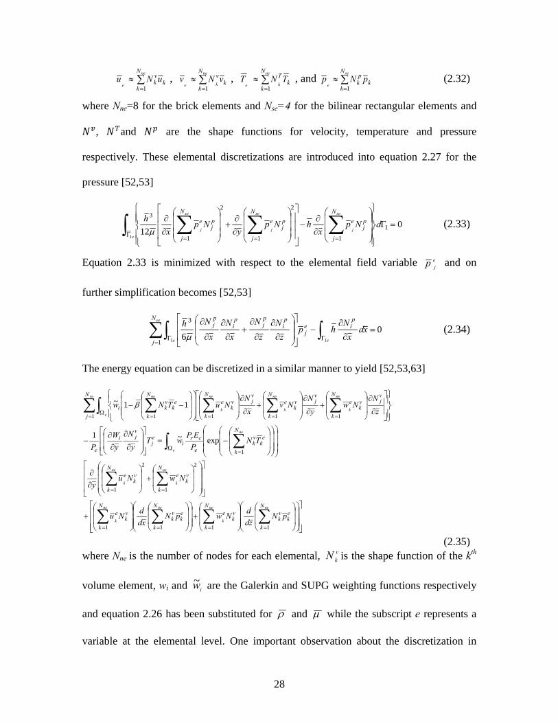
28
∑=
≈ne
e
N
kk
vk uNu
1, ∑
=≈
ne
ke
N
kk
vvNv1
, ∑=
≈ne
ke
N
kk
TTNT1
, and ∑=
≈se
e
N
kk
pk pNp
1 (2.32)
where Nne=8 for the brick elements and Nse=4 for the bilinear rectangular elements and
, and are the shape functions for velocity, temperature and pressure
respectively. These elemental discretizations are introduced into equation 2.27 for the
pressure [52,53]
∫ ∑∑∑Γ ===
=Γ
⎪⎪⎭
⎪⎪⎬
⎫
⎪⎪⎩
⎪⎪⎨
⎧
⎟⎟⎟
⎠
⎞
⎜⎜⎜
⎝
⎛
∂∂
−⎥⎥⎥
⎦
⎤
⎢⎢⎢
⎣
⎡
⎟⎟⎟
⎠
⎞
⎜⎜⎜
⎝
⎛
∂∂
+⎟⎟⎟
⎠
⎞
⎜⎜⎜
⎝
⎛
∂∂
e
se
j
se
j
se
jdNp
xhNp
yNp
xh
N
j
pj
eN
j
pj
eN
j
pj
e
1
012 1
1
2
1
2
1
3
μ (2.33)
Equation 2.33 is minimized with respect to the elemental field variable ejp and on
further simplification becomes [52,53]
∫∑∫ Γ=
Γ=
∂∂
−⎥⎥
⎦
⎤
⎢⎢
⎣
⎡
⎟⎟
⎠
⎞
⎜⎜
⎝
⎛
∂∂
∂
∂+
∂∂
∂
∂
e
se
e
xdx
Nhp
zN
zN
xN
xNh p
iej
N
j
pi
pj
pi
pj
11
06
1
3
μ (2.34)
The energy equation can be discretized in a similar manner to yield [52,53,63]
⎥⎥⎥
⎦
⎤
⎢⎢⎢
⎣
⎡
⎟⎟⎟
⎠
⎞
⎜⎜⎜
⎝
⎛
⎟⎟
⎠
⎞
⎜⎜
⎝
⎛
⎟⎟
⎠
⎞
⎜⎜
⎝
⎛+
⎟⎟⎟
⎠
⎞
⎜⎜⎜
⎝
⎛
⎟⎟
⎠
⎞
⎜⎜
⎝
⎛
⎟⎟
⎠
⎞
⎜⎜
⎝
⎛+
⎥⎥⎥
⎦
⎤
⎢⎢⎢
⎣
⎡
⎟⎟⎟
⎠
⎞
⎜⎜⎜
⎝
⎛
⎟⎟
⎠
⎞
⎜⎜
⎝
⎛+⎟
⎟
⎠
⎞
⎜⎜
⎝
⎛
∂∂
⎟⎟⎟
⎠
⎞
⎜⎜⎜
⎝
⎛
⎟⎟⎟
⎠
⎞
⎜⎜⎜
⎝
⎛
⎟⎟
⎠
⎞
⎜⎜
⎝
⎛−=
⎥⎥⎦
⎤
⎢⎢⎣
⎡
⎟⎟
⎠
⎞
⎜⎜
⎝
⎛
∂
∂
∂∂
−
⎪⎭
⎪⎬⎫
⎪⎩
⎪⎨⎧
⎥⎥
⎦
⎤
⎢⎢
⎣
⎡
∂
∂⎟⎟
⎠
⎞
⎜⎜
⎝
⎛+
∂
∂⎟⎟
⎠
⎞
⎜⎜
⎝
⎛+
∂
∂⎟⎟
⎠
⎞
⎜⎜
⎝
⎛
⎟⎟⎟
⎠
⎞
⎜⎜⎜
⎝
⎛
⎟⎟
⎠
⎞
⎜⎜
⎝
⎛−−
∑∑∑∑
∑∑
∑∫
∑∫ ∑∑∑∑
====
==
=Ω
=Ω
====
nene
k
nene
k
ne
k
ne
k
ne
e
ve
e
ne
k
ne
k
ne
k
ne
N
k
ek
vk
N
k
vk
eN
k
ek
vk
N
k
vk
e
N
k
vk
eN
k
vk
e
N
k
ek
vk
e
cri
ej
vji
e
N
j
vj
N
k
vk
evj
N
k
vk
evj
N
k
vk
eN
k
ek
vki
pNzd
dNwpNxd
dNu
NwNuy
TNPEPwT
yN
yW
P
zN
Nwy
NNv
xN
NuTNw
1111
2
1
2
1
1
1 1111
exp~1
11~ β
(2.35) where Nne is the number of nodes for each elemental, v
kN is the shape function of the kth
volume element, wi and iw~ are the Galerkin and SUPG weighting functions respectively
and equation 2.26 has been substituted for ρ and μ while the subscript e represents a
variable at the elemental level. One important observation about the discretization in

29
equation 2.35 is that the gradient pressure vectors xp ∂∂ / and zp ∂∂ / on boundary Γ1 have
to be extended into the volume domain Ω in order to compute the velocity components u
and v (figure 2.4b). The governing equations are used to develop the model using the
finite element program Sepran [62], an FE program developed at Delft University. The
program is structured into ‘standard problems’ that mainly encompass solution to second-
order elliptic and parabolic differential equations. One advantage the program has is the
ease with which user subroutines are implemented in the Fortran programming language.
An example is the computation of compressibility terms in equation 2.35, velocity
components u, v, and w, effective viscosity μeff and density ρ.
Performance parameters are the load capacity, frictional drag force, and side flow. The
non-dimensional load carrying capacity and frictional force for a slider are [9]
∫ ∫ ⎥⎥⎦
⎤
⎢⎢⎣
⎡⎥⎦
⎤⎢⎣
⎡∂∂
−⎭⎬⎫
⎩⎨⎧
∂∂
∂∂
+⎭⎬⎫
⎩⎨⎧
∂∂
∂∂1
0
1
0 0
12
322
3 4 zdxdFFh
xzpFh
zxpFh
x sλ (2.36a)
(2.36b)
where velocity component is determined in Appendix A and is the
differential of equation A_2 with respect to y.
Shaft frictional torque Tfr in journal bearings is determined by integrating shear stresses
( / at the shaft and bush interfaces [54]
(2.37)
where velocity components and are presented in Appendix A. The first term is due
to film pressure and second due to velocity-induced shearing. Load capacity for journal

30
bearings is presented in section 2.4. Equations 2.36 and 2.37 were solved using user
subroutine which performs the integrations using current values of viscosity μ .
The flow rate has a pressure and velocity-induced component [64]
(2.38)
where is determined in appendix A. Side flow in slider bearings can also be determined
by assuming conservation of mass flow and finding the difference between the inflow
and outflow, oiL QQQ −= .
2.4 Modeling Procedure
The equations presented in sections 2.2 and 2.3 form the core of the bearing template
developed. A flow chart of the implementation is shown in figure 2.5. Current values of
viscosity μ are used to compute the pressure field from Reynolds equations (2.5 and
2.8) with the boundary conditions equations 2.7 and 2.9. A conjugate gradient iteration
method is used. The pressure is used in the next step where the Reynolds equation is
solved with the Swift-Stieber boundary condition using an over-relaxation technique with
constraint p≥0. Two important forces on the bearing are the load capacity as determined
from the Reynolds equation Wd and the actual load W. A force balance must exist
between the applied load and load capacity. The procedure used to achieve this is
a. Assume an initial value for eccentricity e, compute eccentricity ratio (ε=e/c)
(normal range 0.5≤ε≤0.9) as well as attitude angle ϕ and compute the film
thickness h(θ) from (see figure 2.1b)
h(θ)=c(1+εcos(θ-ϕ)) (2.39a)

31
where c=(R1-R2) is the radial clearance, θ and ϕ the angle from the load line and
attitude angle respectively. The minimum film thickness is located at θ=π+ϕ
hmin=c(1-ε) (2.39b)
b. Solve the Reynolds equation for pressure and load-carrying capacity Wd.
c. For this capacity compute the reaction load fR=(fx,fz)T and attitude angle from
( )∫ΩΩ−= dpf x ϕcos (2.40a)
( )∫ΩΩ−= dpf z ϕsin (2.40b)
and fR (2.40c)
and attitude angle ϕ which is
⎟⎠⎞
⎜⎝⎛= −
z
y
ff1tanϕ (2.40d)
Sommerfeld number can be computed from
2
⎟⎠⎞
⎜⎝⎛=
CR
WDLN
S seffμ
(2.40e)
d. If fR<W increase the value of eccentricity ratio ε, if fR>W decrease its value.
e. Compute the attitude angle from equation 2.40d. If ϕ<ϕa (where ϕa is value from
step a) decrease value of ϕ (in step a), or if ϕ>ϕa increase value of ϕ (in step a).
f. Go back to step a and repeat procedure.
g. When convergence is obtained on both eccentricity ratio and attitude angle, the
flowchart in figure 2.5 continues at stage 4 by computing velocity components u,
v, w.
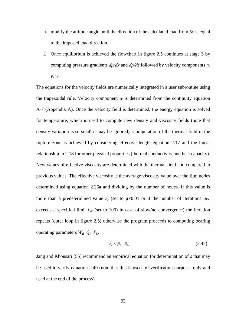
32
h. modify the attitude angle until the direction of the calculated load from 5c is equal
to the imposed load direction.
i. Once equilibrium is achieved the flowchart in figure 2.5 continues at stage 3 by
computing pressure gradients dp/dx and dp/dz followed by velocity components u,
v, w.
The equations for the velocity fields are numerically integrated in a user subroutine using
the trapezoidal rule. Velocity component w is determined from the continuity equation
A-7 (Appendix A). Once the velocity field is determined, the energy equation is solved
for temperature, which is used to compute new density and viscosity fields (note that
density variation is so small it may be ignored). Computation of the thermal field in the
rupture zone is achieved by considering effective length equation 2.17 and the linear
relationship in 2.18 for other physical properties (thermal conductivity and heat capacity).
New values of effective viscosity are determined with the thermal field and compared to
previous values. The effective viscosity is the average viscosity value over the film nodes
determined using equation 2.26a and dividing by the number of nodes. If this value is
more than a predetermined value εr (set to μ≤0.01 or if the number of iterations iter
exceeds a specified limit Lm (set to 100) in case of slow/no convergence) the iteration
repeats (outer loop in figure 2.5) otherwise the program proceeds to computing bearing
operating parameters , , .
1−−≤ iir μμε (2.42)
Jang and Khonsari [55] recommend an empirical equation for determination of ε that may
be used to verify equation 2.40 (note that this is used for verification purposes only and
used at the end of the process).

33
( )SDL
ln20986.0/
49737.036667.0 −+−=ε for 0.5 ≤ L/D ≤ 1.5 (2.41)
Periodical boundary conditions are applied to surfaces S3 and S5 in figure 2.3. Similar
conditions are set for the bush and shaft ends.
A typical run using data from Dowson et al. [59] is given below
a. Initial guesses: ε=0.5, ϕ=0.9 radians.
b. Initial results from solving Reynolds: horizontal component of load fx: 2.81838E+03 vertical component of load fy: 4.94780E+03 modulus of load fR: 5.69421E+03 attitude angle: 1.05301E+00
c. W=11 000N, therefore W>fR increase ε to 0.64. Second iteration gave the results horizontal component of load 7.05888E+03 vertical component of load 8.51415E+03 modulus of load 1.10598E+04 attitude angle 8.78576E-01
Third iteration with ε=0.63: horizontal component of load 7.24169E+03 vertical component of load 8.28417E+03 modulus of load 1.10032E+04 attitude angle 8.52443E-01
The modulus of load or fR=11 003 ≈ W; the iterations can be stopped. The flowchart continues at stage 4 in figure 2.5.
2.5 Chapter summary
The streamline upwind Petrov-Galerkin finite element method is formulated for three-
dimensional thermo-hydrodynamic lubrication problems. Governing equations and
boundary conditions in the critical areas of the groove and rupture zone are presented.
The model is used to simulate slider bearings thermal behavior in chapter 3 and journal
bearings in chapter 4.

34
Figure 2.5 Flowchart for thermo-hydrodynamic lubrication model.
Start. Input parameters Ti, μa,, n, k,ρ, D, C
Find gradients ∂p/∂x, ∂p/∂y
Compute the velocity components u, v, w using Navier-Stokes and
continuity equations
Use current value of μ to compute p using constrained minimization and over-relaxation. Determine ε, h, ϕ (eqns. 2.39-2.40) at force
balance equilibrium
Compute new pressure field pnew with updated viscosity , frictional torque Tr, power loss PL,, QL for current values of viscosity
Is |µnew-µold|≤εr Or is
Iter>Lm
Yes
No
Compute output parameters rT , LQ and solve for conduction in pad/bush
End
Compute new viscosity and density fields
Change value of θ?
No
Yes
Solve energy equation iteratively for temperature field T in film. Use conduction eqn to determine temperature in pad/bush

35
Chapter 3
Application of SUPG FE to Slider Bearings
3.1 Introduction
The streamline upwind Petrov-Galerkin (SUPG) finite element method formulated in
chapter 2 is chosen for its robust nature and rapid convergence in convection dominated
flows. The method is applied to slider bearings analysis and design in this chapter.
Slider bearings are widely used in applications such as mechanical seals, collar thrust
bearings, machine tool guides, and piston rings. They have good load-carrying capacity,
excellent stability and durability. A tilted pad slider bearing consists of two surfaces as
shown in figure 2.1a separated by a lubricant film. The direction of the runner motion and
inclination of the planes are such that a converging oil film is formed between the two
surfaces and the physical wedge pressure-generating mechanism is developed in the
lubricant film. This enables the bearing to support a load. The flow is viscous, leading to
heat generation, dissipation and increase in film temperature.
3.2 Lebeck Slider Bearing Data
The test case presented by Lebeck [65] and used by Kumar [9] in a two-dimensional
model with input values in Table 3.1 is used. Mesh density sensitivity analysis was
performed with the thermo-hydrodynamic SUPG model; results appear in Table 3.2. The
maximum number of pressure and temperature iterations for convergence is also
indicated. An analytical load capacity is included and used as a benchmark. A 30x30x10
(x-y-z) mesh is finally chosen. The length (x) and height (y) values are similar to those
used by Kumar [9] while an axial value of ten elements is a good compromise in
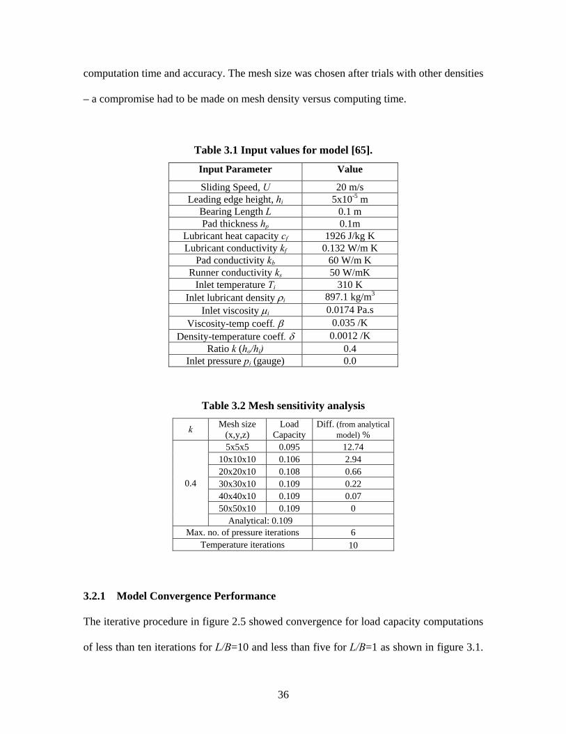
36
computation time and accuracy. The mesh size was chosen after trials with other densities
– a compromise had to be made on mesh density versus computing time.
Table 3.1 Input values for model [65].
Input Parameter Value
Sliding Speed, U 20 m/s Leading edge height, hi 5x10⁻⁵ m
Bearing Length L 0.1 m Pad thickness hp 0.1m
Lubricant heat capacity cf 1926 J/kg K Lubricant conductivity kf 0.132 W/m K
Pad conductivity kb 60 W/m K Runner conductivity ks 50 W/mK
Inlet temperature Ti 310 K Inlet lubricant density ρi 897.1 kg/m3
Inlet viscosity μi 0.0174 Pa.s Viscosity-temp coeff. β 0.035 /K
Density-temperature coeff. δ 0.0012 /K Ratio k (ho/hi) 0.4
Inlet pressure pi (gauge) 0.0
Table 3.2 Mesh sensitivity analysis
k Mesh size (x,y,z)
Load Capacity
Diff. (from analytical model) %
0.4
5x5x5 0.095 12.74 10x10x10 0.106 2.94 20x20x10 0.108 0.66 30x30x10 0.109 0.22 40x40x10 0.109 0.07 50x50x10 0.109 0
Analytical: 0.109 Max. no. of pressure iterations 6
Temperature iterations 10
3.2.1 Model Convergence Performance
The iterative procedure in figure 2.5 showed convergence for load capacity computations
of less than ten iterations for L/B=10 and less than five for L/B=1 as shown in figure 3.1.

37
Table 3.3 has the limiting values for the outer loop in figure 2.5 and an indication of the
convergence values. The power and advantage of SUPG is evident in the finite bearing
case where, at L/B=1 convergence takes place after only three iterations. A similar
pattern is evident in journal bearing simulations.
Figure 3.1 Convergence of load capacity solution.
Table 3.3 Convergence criteria
Maximum number of iterations – outer loop 15 Percentage variation – 1st to 2nd iteration 57.9 Percentage variation – 5th to 6th iteration 4.9
Pressure iteration: max no. 6 Temperature iterations: 10
Load Capacity as Function of Number of Iterations
0.00E+00
2.00E+05
4.00E+05
6.00E+05
8.00E+05
1.00E+06
1.20E+06
1.40E+06
1 2 3 4 5 6 7 8 9 10
Number of iterations
Load
Cap
acity
, N/m
2
L/B=10L/B=5L/B=3L/B=2L/B=1

38
3.2.2 Predicted Pressure Values
The effect of the width to length ratio L/B on predicted pressures generally indicates
whether a bearing is infinite or finite. Initially adiabatic conditions on upper and lower
surfaces and an inlet temperature Ti=To are assumed. The 3-D SUPG model formulated
in section 2.5 is used to predict peak pressure and load capacity. Results appear in table
3.4 and figure 3.2. Values of peak pressure for L/B ratios of ∞ (2-D model), 20, 10, and 5
are coincident as expected [66]. Percent difference in table 3.4 indicates model
predictions for the infinitely wide (2-D) and 3-D sliders as a function of L/B ratio for both
peak pressure and load capacity. Both fall dramatically at L/B values less than 2. What is
significant here is the sudden drop in load carrying capacity from L/B of 2 to 1 (square
slider). A 3-D model should be used for L/B less than 3.
Table 3.4 Isothermal peak pressure and load capacity, k=0.4
L/B ratio
Peak Pressure
( p )
Difference
(%)
Load capacity
W
Difference to 2D
model (%) 2D Model 0.2564 - 1.572 -
20 0.2564 0.00 1.572 0 10 0.2564 0.00 1.572 0 5 0.2562 0.09 1.571 0.06 2 0.2378 7.3 1.453 7.5 1 0.1669 34.9 0.9996 36.4
0.5 0.0806 68.6 0.4437 71.8

39
0.00
0.05
0.10
0.15
0.20
0.25
0.30
0.00 0.10 0.20 0.30 0.40 0.50 0.60 0.70 0.80 0.90 1.00
x/L
SUPG Predictions as function of L/B ratio
p_2D
p_20:1
p_10:1
p_5:1
p_2:1
p_1:1
p_0.5:1
Figure 3.2 Non-dimensional isothermal pressure predictions as a function of L/B. The first four lines (L/B=∞, 20, 10, 5) coincide.
Arnell [66] suggests sliders are considered finite when L/B<2 which corresponds to a
peak pressure difference of 7%. Of more significance is the thermo-hydrodynamic effect
on peak pressure predictions as shown in Table 3.5 which indicates the difference
between isothermal and THD values for several L/B ratios. Consideration of the thermo-
hydrodynamic effect must be made at the bearing speed tested (20 m/s).
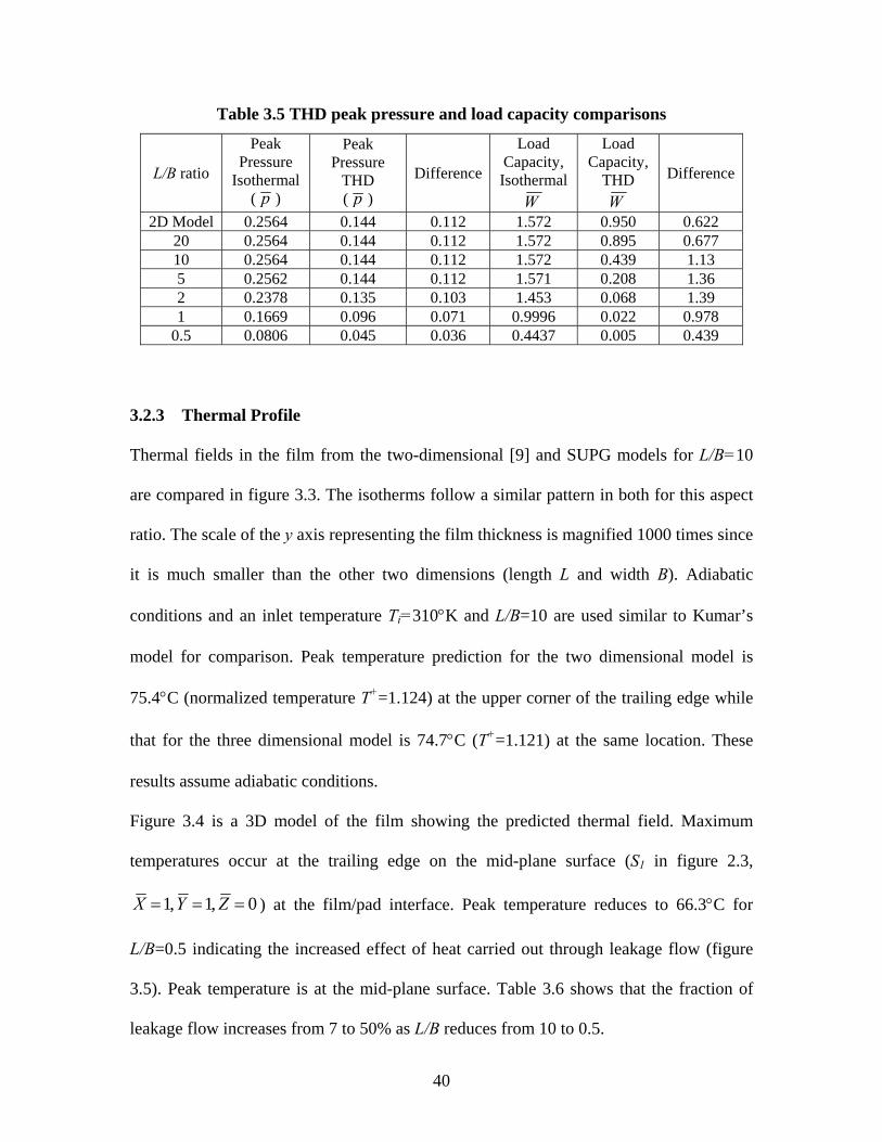
40
Table 3.5 THD peak pressure and load capacity comparisons
L/B ratio
Peak Pressure
Isothermal ( p )
Peak Pressure
THD ( p )
Difference
Load Capacity, Isothermal
W
Load Capacity,
THD W
Difference
2D Model 0.2564 0.144 0.112 1.572 0.950 0.622 20 0.2564 0.144 0.112 1.572 0.895 0.677 10 0.2564 0.144 0.112 1.572 0.439 1.13 5 0.2562 0.144 0.112 1.571 0.208 1.36 2 0.2378 0.135 0.103 1.453 0.068 1.39 1 0.1669 0.096 0.071 0.9996 0.022 0.978
0.5 0.0806 0.045 0.036 0.4437 0.005 0.439
3.2.3 Thermal Profile
Thermal fields in the film from the two-dimensional [9] and SUPG models for L/B=10
are compared in figure 3.3. The isotherms follow a similar pattern in both for this aspect
ratio. The scale of the y axis representing the film thickness is magnified 1000 times since
it is much smaller than the other two dimensions (length L and width B). Adiabatic
conditions and an inlet temperature Ti=310°K and L/B=10 are used similar to Kumar’s
model for comparison. Peak temperature prediction for the two dimensional model is
75.4°C (normalized temperature T+=1.124) at the upper corner of the trailing edge while
that for the three dimensional model is 74.7°C (T+=1.121) at the same location. These
results assume adiabatic conditions.
Figure 3.4 is a 3D model of the film showing the predicted thermal field. Maximum
temperatures occur at the trailing edge on the mid-plane surface (S1 in figure 2.3,
0,1,1 === ZYX ) at the film/pad interface. Peak temperature reduces to 66.3°C for
L/B=0.5 indicating the increased effect of heat carried out through leakage flow (figure
3.5). Peak temperature is at the mid-plane surface. Table 3.6 shows that the fraction of
leakage flow increases from 7 to 50% as L/B reduces from 10 to 0.5.

41
More industrially applicable conditions, such as those used by Kumar [9]: 0.1=ip ,
)372(2.1 KTi =+ , )434(4.1 KTp =+ and )310(0.1 KTs =+ are used to run the model. These
normalized temperatures are relative to the inlet temperature in °K, all other variables are
in Table 3.1). Inflow boundary conditions were checked and updated as well as using a
finer grid mesh N=30x30x30 with improved results as shown in figure 3.6a. A clearer
picture emerges when predictions are compared to Kumar’s results by digitizing and
superimposing these onto figure 3.6a. Figure 3.6b shows a couple of isotherms. What is
evident from this is that although relatively close, it is difficult to reproduce Kumar’s
results exactly. Isotherms generally follow similar patterns in both cases although model
predictions appear to be shifted slightly upwards especially at the lower regions.

42
Figure 3.3(a) Normalized temperatures for 2-D and (b) 3-D SUPG models showing
general patterns of the isotherms.
(a)
(b)

43
Figure 3.4 Contour map of the thermal field, L/B=10 (hi=50μm). The arrow shows flow
direction.
Y+
0
0
.2
0
.4
0.6
0.8
1

44
Figure 3.5 Thermal field with L/B=0.5 (hi=50μm).
0
0.2
0.4
0
.6
0
.8
1
Y+

45
(a)
(b)
Figure 3.6(a) Model isotherms for Lebeck’s data [65] (b) Comparison of temperature profiles from SUPG model (solid lines) and Kumar [9] (dashed lines).

46
3.2.4 Leakage Flow Pattern – Flow Gradient Method
The SUPG model is used to predict flow patterns as a function of L/B in more detail.
Table 3.6 shows the average side flow as a function of L/B, also shown in figure 3.7 for
0.1<k<0.9 and different L/B ratios. Flow is determined at k intervals of 0.1 and averaged
out. Boxed numbers represent the ratio of side leakage to inflow as a percentage. It
increases significantly for L/B ratios less than two. The values presented in table 3.6 and
figure 3.7 are for average dimensionless flow rates for the range 0.1<k<0.9 and represents the
general behavior of slider bearings as a function of aspect ratio L/B. Figure 3.8 follows from the
general observations evident from figure 3.7 and is applicable to slider bearings in general.
The gradient in figure 3.8 is determined manually at each point on figure 3.7. A
differencing technique is used to compute the change in tilt ratio d(L/B) and flow .
The gradient gives an indication of how the flow is changing as a function of length to
width ratio L/B. The minimum point IP represents, for a given tilt angle k, rate of change
of leakage flow as a function of L/B ratio is zero. This point is at L/B=2 in figure 3.8.
Lower values of the L/B give more leakage flow but far less load-carrying capacity
whereas higher L/B values give more load capacity but less leakage flow and
consequently higher operating temperatures. Thus Ip gives a good compromise between
load capacity and leakage flow for optimum operating temperature. As pointed out earlier
higher leakage flows are beneficial in lowering peak operating temperatures.
The gradient of side flow ∂QL/∂(L/B) is high from zero to L/B=1, decreases rapidly
between L/B=1 and L/B=2 to almost zero, gradually increases from two to ten, then
becomes nearly constant above ten. It decreases rapidly from zero to one. It can be
argued that the influence of side flow is most significant between zero and two. Even
though load capacities are relatively low in this region, the beneficial effects of lower

47
operating temperatures are realized. Another interesting observation is that even at
L/B=60 the percentage of side flow to inlet flow is 4.9 although the slider is in the
infinite range.
Figure 3.8 illustrates the Flow Gradient Method of determining optimum leakage flow by
computing the gradient Qd / ( )BLd / for 0.1<k<0.9. The graph bottoms out at a ratio of
two, increases up to a ratio of ten and remains nearly constant thereafter. To the best of
our knowledge this work represents the first definition of the Flow Gradient Method.
Table 3.6 Dimensionless flow rate as a function of L/B1
L/B
vQ
oQ
LQ
Ratio of side leakage to inflow, %
60 46.4 44.1 2.3 4.9 40 30.9 29.4 1.6 5.1 20 15.5 14.7 0.87 5.6 10 7.86 7.29 0.57 7.2 5 4.05 3.60 0.46 11.2 2 1.79 1.37 0.42 23.3 1 1.02 0.63 0.39 38.0
0.5 0.57 0.29 0.28 49.7 0.25 0.30 0.13 0.17 55.4
, , and are the inflow, outflow and side leakage flow respectively

F
0.
0.
1.
1.
2.
2.
3
igure 3.7 Dinumbe
.0
.5
.0
.5
.0
.5
0
55.449.7
38.0
23.311.2
0
0.05
0.1
0.15
0.2
0.25
0.3
0.35
0.4
0.45
0.5
0
imensionlessers represent
Fig
10
Dimens
7.2
0 2 4 6
Flow G
s side leakagthe ratio of
gure 3.8 Flow
20Leng
sionless leak
5.6
8 10 12 1
Gradient a
48
ge LQ as a fuside leakage
w gradient,
30gth to width rati
kage flow as
14 16 18 20L/B
as Functio
unction of L/e to inflow a
0.1<k<0.9.
40o L/B
function of L
5.1
0 22 24 26 2
on of L/B,
/B, 0.1<k<0as a percenta
50
L/B, 01<k<0.
28 30 32 34
, 0.1<k<0
dQ/d(L/B
.9. Boxed age.
60
.9
-
4.9
4 36 38 40
.9
)

49
In Figure 3.9 the non-dimensional side leakage pattern from point A to B in figure 2.3a is
shown as a function of L/B for k=0.4. Numbers in boxes indicate the width to length ratio
L/B. Side leakage increases from L/B=20 to a peak at L/B=1 and L/B=2 then declines as
L/B decreases. This is an important observation, as it implies the bearing is optimized in
terms of side leakage in the range L/B=1-2.
Figure 3.9 Side leakage as a function of L/B, k=0.4.
Although the fact that finite sliders run at significantly lower temperatures than higher
width ones has been long established [67] the effect on the point of the most intense
viscous dissipation has not been widely reported. Peak temperature increase lowers
lubricant viscosity which leads to lower load carrying capacity. Slider geometry can be
Side leakage profiles
0.00
0.05
0.10
0.15
0.20
0.25
0 0.1 0.2 0.3 0.4 0.5 0.6 0.7 0.8 0.9 1
Non
-dim
ensi
onal
leak
age
flow
L/B=20L/B=10L/B=1L/B=0.5L/B=2L/B=3
L/B=20
10
0.5
1 2
3

50
adjusted or new geometries can be tried in order to reduce the effect of higher
temperatures on load carrying capacity.
The effect of tilt ratio k on peak temperatures and load carrying capacity are shown in
figure 3.10 for L/B of 20, 10, 5, and 1. All variables not specified are in Table 3.1. Boxed
numbers show peak temperature predictions at each k value. A high tilt angle (low k
value) results in high peak temperatures. The highest load capacity occurs at k=0.5 in
both cases. Even though high values of k have a lower peak temperature, load capacity is
less. A tilt ratio of 0.5 seems ideal for slider design, although slightly higher values
(k=0.6-0.7) are preferred for their lower peak temperatures. The high peak temperatures
at L/B=10 and 20 and tilt ratio k=0.1 suggest high risk of metal to metal contact for these
values.
Figure 3.10 Load capacity as a function of k. Non-dimensional load capacity is as defined
in nomenclature.
0.00
0.10
0.20
0.30
0.40
0.50
0.60
0.70
0.80
0.90
1.00
0 0.1 0.2 0.3 0.4 0.5 0.6 0.7 0.8 0.9 1
Non
Dim
Loa
d C
apac
ity
Parameter k
Load Capacity as a Function of k
L/B=10
L/B=1
L/B=5
L/B=20
64 C69 C
49 C
82 C
75 C69 C 64 C
61 C
58 C
56 C
58 C
87 C
61 C
77 C 71 C 66 C 62 C 59 C 57C 56 C
75 C
82 C
75 C
69 C64 C
61 C
58 C
56 C
55 C
56 C
83 C

51
3.3 Chapter Summary
The three dimensional SUPG thermo-hydrodynamic model developed is used to analyze
slider bearing characteristics at different width to length and tilt ratios. Pressure
predictions for the non-isothermal case are significantly less than the isothermal case as
expected. Model predictions show square sliders running at lower temperatures than
wider ones. This is due to the higher side leakage; however their load carrying capacity is
significantly less. The significance of side leakage on peak temperature is evident. The
model also shows that side leakage peaks in the region L/B=1-2. The Flow Gradient
Method to predict optimum flow conditions is proposed. Even though high values of the
tilt ratio have a lower peak temperature, the load capacity is less and an tilt ratio of 0.5-
0.7 seems ideal for slider design. Lower peak temperatures are predicted if inlet pressure
is raised from ambient to 0.1=ip . Ways to do this should be implemented on slider
bearing if higher load capacities are required.

52
Chapter 4
Streamline Upwind Petrov-Galerkin FE and Journal Bearings
4.1 Introduction
The streamline upwind Petrov-Galerkin finite element for thermo-hydrodynamic
modeling is used for the analysis and design of journal bearings. Theoretical basis of the
model applicable to plain journal bearings with requirements to account for cavitation
effects was presented in chapter 2. A novel THD template for journal bearings in
Cartesian coordinates that shows good convergence is developed.
4.2 Model Formulation
Figure 4.1(a) shows the classical two-dimensional journal geometry while figure 4.1(b)
illustrates the model development whereby the bearing is unwrapped into regions that
correspond to the bush, fluid and shaft. The oil groove presents a good reference point
whereas attitude angle φ (fig 4.1(a)) depends on bearing load and speed among other
factors. The computational region for pressure is mapped onto a rectangle, the x-z plane
while the y axis represents the film thickness h as a function of angle θ from groove
position. The minimum film thickness hmin is at an angle ϕ from the groove position as
illustrated in figure 4.1a. Figure 4.2 shows the fluid region where film thickness h is a
function of the x-coordinate. The cutting plane splits the oil groove in half. Periodic
boundary conditions identify surfaces S3 and S5 as ‘mating’, representing the circular
nature of the template.

53
The film thickness h is determined from equation 2.39. The film thickness h(θ) from
equation 2.39 can be transformed to h(x) from the relation h(x)= h(θ)/(πD).
Figure 4.1(a) Schematic representation of journal bearing.
4.1(b) Journal bearing unwrapped. The cross-sectional areas of the two regions are equal
BushFluid region (exaggerated) Shaft
ϕ
eR1
R2
Oil supply hole
h
W
yb xb
θ
y
x
z
ωR3
Oil groove
fys
fxs
xsys

54
4.1(c) Isometric view of finite element mesh of the model
Figure 4.2 Cross section of the film region. Note that the origin is on line C3 and surfaces S3 and S5 are defined on C4 and C3 respectively.
Z
Y
X
Journal (lower surface)
bush Oil grooves
Mid-plane surface S1
Side surface S3
Side surface S5
C1
End surface S4
C2
ps bc’s
C3
C4x

55
Film rupture and reformation effects have to be considered in journal bearing
computations. Cavitation algorithms fall into two main categories, the Swift-Stieber
(Reynolds) boundary condition which states that ∂p/∂ϕ=0 at ϕ=ϕcav, where ϕcav is the
rupture interface, and the mass conserving algorithms by Elrod [28] and Kumar and
Booker [29,30] among others. The Swift-Stieber condition has gained wide acceptance
for steady state stationary loaded journal bearings [55] even though it does not work as
well at the reformation boundary, will be used.
4.3 Simulation Results
4.3.1 Mesh Density, Convergence and Performance
The experimental data from Dowson [59] represents one of the landmark work in plain
journal bearings and is often used to validate many journal bearing models. Initial model
validation was performed on this data. Input parameters and thermocouple setup
information is given in table D.1 and section D1.1. The same problem is solved
analytically by Khonsari [68] using the Boyd and Raimondi tables and Yang and
Khonsari’s [55] proposed empirical equations. No data on the bush dimensions and
geometry of the oil supply groove thus a convective heat transfer coefficient for the
bush/ambient interface of 100W/m2.K is used and found to give results close to
experimental. The published peak pressure of 3.5 MPa obtained by Dowson [59] is used
in convergence analysis. Table 4.1 shows the effect of varying grid size from N=10x10 to
N=80x80 for both linear and quadratic elements. The sequence N=10x10, 20x20 …is
used since it is recommended in numerical analysis to halve the step size in a
convergence study. As expected quadratic elements converge faster although they are
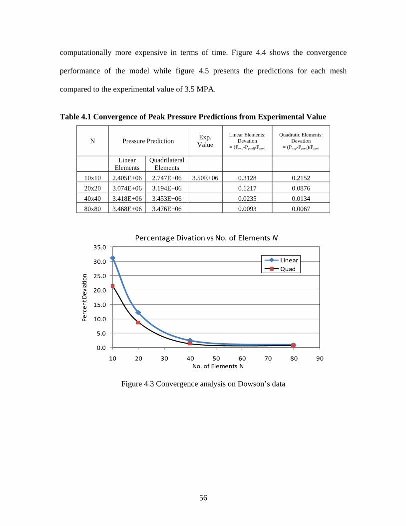
56
computationally more expensive in terms of time. Figure 4.4 shows the convergence
performance of the model while figure 4.5 presents the predictions for each mesh
compared to the experimental value of 3.5 MPA.
Table 4.1 Convergence of Peak Pressure Predictions from Experimental Value
N Pressure Prediction Exp. Value
Linear Elements: Devation
= (Pexp-Ppred)/Ppred
Quadratic Elements: Devation
= (Pexp-Ppred)/Ppred
Linear Elements
Quadrilateral Elements
10x10 2.405E+06 2.747E+06 3.50E+06 0.3128 0.2152 20x20 3.074E+06 3.194E+06 0.1217 0.0876 40x40 3.418E+06 3.453E+06 0.0235 0.0134 80x80 3.468E+06 3.476E+06 0.0093 0.0067
Figure 4.3 Convergence analysis on Dowson’s data
0.0
5.0
10.0
15.0
20.0
25.0
30.0
35.0
10 20 30 40 50 60 70 80 90
Percen
t Deviatio
n
No. of Elements N
Percentage Divation vs No. of Elements N
LinearQuad

57
Figure 4.4 Peak pressure prediction for Dowson’s experimental value of 3.5 MPa
Quadratic element mesh achieves a deviation of only 1.3% with a 40x40 mesh size while
an 80x80 mesh is required for linear ones. Computation times as a function of mesh
density for linear elements are shown in table 4.2 (using a Pentium IV 3.25 GHz 1 GB
RAM). These are for a single iteration in figure 2.5. Considering that each cycle required
at least three iterations for convergence and that the process is repeated at Ns=2 rev/s
intervals in the optimization model, computation time can be considerable. A target
deviation of 1% was used which coincides with a mesh of N=80x80 elements (0.9%).
Table 4.2 Computation Times for One Iteration
Computation Times (Sec)
N Mesh Computing Total
10x10 0.0313 0.0156 0.046920x20 0.0781 0.0469 0.125 40x40 0.2812 0.4219 0.703180x80 1.0156 1.9219 2.9375
0.0
0.5
1.0
1.5
2.0
2.5
3.0
3.5
4.0
0.0 0.1 0.2 0.3 0.4 0.5 0.6 0.7 0.8 0.9 1.0
Pressure, M
pa
Pressure Predictions vs No. of Elements N
Pressure@N=80x80
Pressure@N=10x10
Pressure@N=20x20
Pressure@N=40x40

58
Model performance in predicting peak temperatures for Dowson’s data is shown figure
4.5 (experimental value is 47°C). In order to compare predicted temperatures to
experimental outlet drain temperatures and Khonsari’s [68] analytical computations,
nodal temperatures are summed and divided by the number of nodes. Khonsari performs
six iterations in his computations as shown in figure 4.5 which also indicates Dowson’s
experimental value and the proposed SUPG model. The rapid convergence of the model
is evident; only three iterations produce stability in predictions. The average temperature
prediction of 48.4˚C from the model is 1.4˚C higher than experimental values; the peak
temperature prediction of 51.2˚C compares favorably with 51.6˚C from Dowson. The
peak temperature is located at the mid-plane of the journal.
Table D.1 (Appendix) has input parameters for the bearing while table 4.3 shows some of
the performance parameter predictions (input parameters not available from Dowson’s
data were estimated). These results are preliminary; more detailed analysis follow.
Figure 4.5 Model, experimental, and analytical predictions, Dowson’s data.
20.0
25.0
30.0
35.0
40.0
45.0
50.0
55.0
60.0
65.0
1 2 3 4 5 6 7
Tem
pera
ture
(C)
No. of Iterations
SUPGThermal Predictions, Analytical Method, and Experimental Temperature
T_measuredT_modelT_analyt
Exp. temperature
Oil inlet

59
Table 4.3 Model predictions, analytical [68] and Dowson’s [59] experimental data.
Analytical SUPG Exp.
Attitude angle ϕ° 51.0 51.0 57.0 Peak Pressure (Mpa) 3.60 3.46 3.50 Side Leakage cm3/s 24.2 26.1 26.2 Friction Force, N 67.4 65.7 64.4 Shaft Torque, N.m 3.42 3.41 3.39
4.3.2 Pressure and Pressure Gradient Predictions
The experimental data from Boncompain et al. [15] and Costa et al. [69] are used to
perform further validation of the model. The top surface is stationary (bush) and the
bottom is the shaft in figure 4.1(b); figure 4.1(c) shows the mesh model. Input parameters
for the bearings appear in Table D.2 and D.3 respectively.
The effect of pressure gradients ∂p/∂x and ∂p/∂z on the energy equation 2.12 is through
the compressibility term (second term on right hand side). This term is retained here even
though most researchers ignore it due to its relatively small contribution [1,2,55,74]. The
behavior of the two gradients near and in the rupture zone form a critical part of the
discussion to follow, hence the need to retain them. Table 4.4 shows the effect of
including the compressibility terms on temperature predictions.
Table 4.4 Effect of pressure gradients ∂p/∂x and ∂p/∂y on temperature rise ΔT
Data Ti, °C ΔT, With
°C ΔT Without, °C Difference, °C
Dowson 36.8 11.39 11.48 0.09 Boncompain 40 11.77 12.13 0.36 Costa 35 19.07 19.19 0.13

60
Model convergence performed on pressure gradient dp/dz for the experimental data from
Boncompain et al. [15] is presented in figure 4.6. The bearing analyzed has aspect ratio
L/B=0.8 which is short and pressure gradient dp/dz falls rapidly from the bearing mid-
plane. Lower values of the gradients at 0.5 are due to the increased effect of film
pressure in the narrowing (converging) part of the bearing.
Pressure predictions from the proposed model and the rupture/reformation interfaces are
shown in figure 4.7 for Boncompain’s [15] bearing. The rupture zone is in the range
00 332227 << θ which is in good agreement with Boncompain’s results (figure 4.7b).
Figure 4.8a presents pressure gradient ∂p/∂x as a function of Z at several locations
around the bearing. Boxed numbers indicate position along the X coordinate. Figure 4.8b
compares ∂p/∂x and ∂p/∂z along the x axis and reveals that the magnitude of ∂p/∂x is
much greater than ∂p/∂z, which is zero except for the rupture zone which consists of
finger-like fluid/gas regions. It appears ∂p/∂x has a contribution on the compressibility
term of the energy equation since it is significantly larger than ∂p/∂z although this
contribution is negligible as indicated in Table 4.3.
4.3.3 Pressure Gradients and Effect on Dissipation
Of more significance is the position of the rupture interface and how it affects the
gradients. The boxed numbers on the ordinate of figures 4.8a and 4.8b show the position
along the x axis for Boncompain’s [15] input data (Table D2 in appendix). The
magnitude of ∂p/∂x increases along the x direction, peaks at 5.0=X , changes sign with a
minimum at 592.0=X which is located just before the rupture interface and becomes
zero at the reformation interface. Noting that the gradients ∂p/∂x and ∂p/∂y are multiplied

61
by the density-temperature coefficient in equation 2.12 and w is several orders of
magnitude less than u [2], the contribution of these gradients to dissipation is minimal
(positive values increase dissipation). Thus investigation of the dissipation phenomenon
from a mathematical point of view gives an insight as to why experimental temperatures
peak just after the rupture interface and decrease thereafter.
Figure 4.6. Convergence analysis on pressure gradient dp/dz.
‐7
‐6
‐5
‐4
‐3
‐2
‐1
0
1
0.0 0.1 0.2 0.3 0.4 0.5 0.6 0.7 0.8 0.9 1.0
dp/dz, MN/m
3
Model Convergence for gradient dp/dz vs No of Elements N
N=10
N=20
N=30
N=50
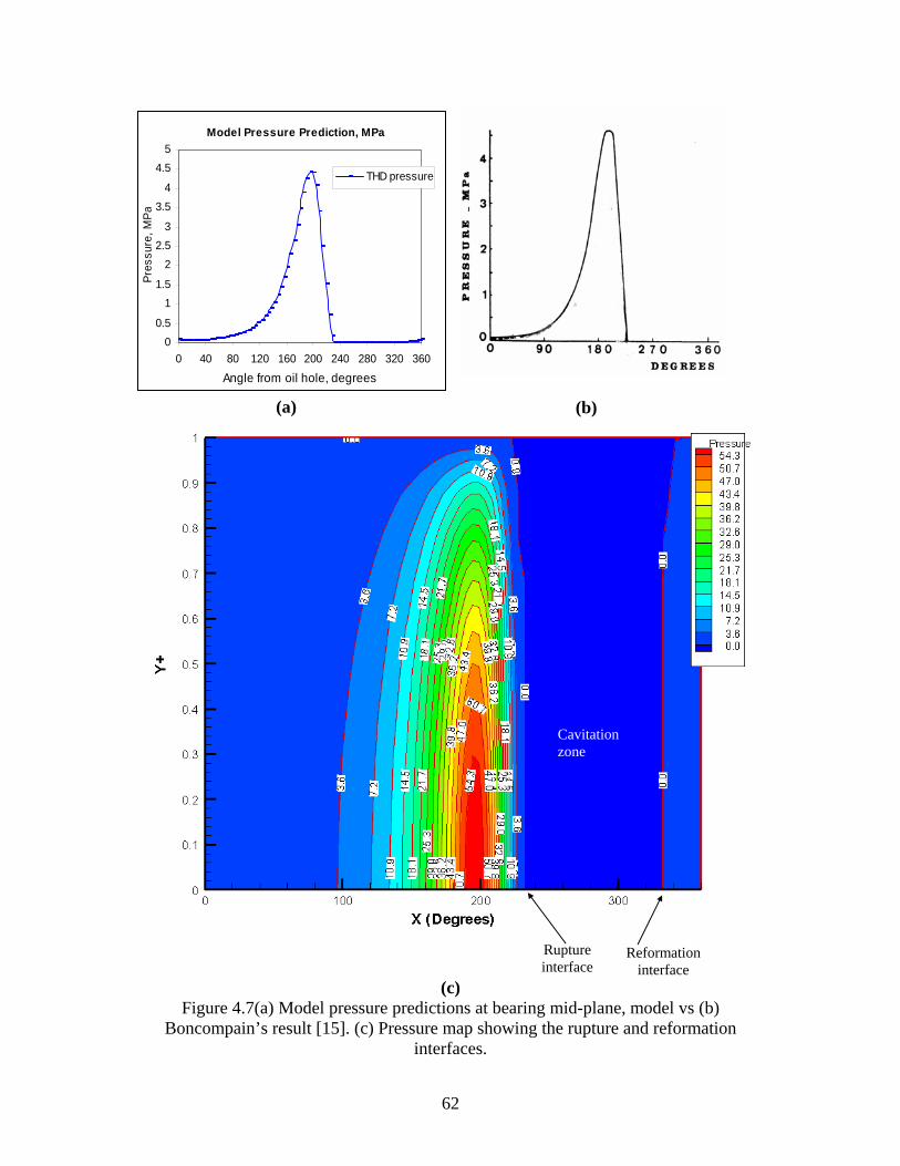
62
(a)
(b)
(c)
Figure 4.7(a) Model pressure predictions at bearing mid-plane, model vs (b) Boncompain’s result [15]. (c) Pressure map showing the rupture and reformation
interfaces.
Model Pressure Prediction, MPa
00.5
11.5
22.5
3
3.54
4.55
0 40 80 120 160 200 240 280 320 360
Angle from oil hole, degrees
Pres
sure
, MPa
THD pressure
Cavitation zone
Rupture interface
Reformation interface

63
(a)
(b)
Figure 4.8(a) Pressure gradient ∂p/∂x variation along the bearing x coordinate, Costa et al. [69]. (b) Pressure gradients ∂p/∂x, ∂p/∂z variation along the x axis.
4.3.4 Dissipation Source Terms
The dissipation source terms (last two terms in equation 2.12) in the energy equation are
evaluated for their contribution to the thermal profile. Figure 4.9 shows the values of the
-250
-200
-150
-100
-50
0
50
100
150
0.00 0.10 0.20 0.30 0.40 0.50
dp/d
x, M
N/m
3
Pressure gradient dp/dx
1. dpdx@X=0.112. dpdx@X=0.213. dpdx@X=0.464. dpdx@X=0.55. dpdx@X=0.536. dpdx@X=0.547. dpdx@X=0.558. dpdx@X=0.619. dpdx@X=0.6510. dpdx@X=0.9211. dpdx@X=0.9912. dpdx@X=0.63
1, 2,10,11
8
12
7
9
6
53
4
‐250
‐200
‐150
‐100
‐50
0
50
100
150
0 0.1 0.2 0.3 0.4 0.5 0.6 0.7 0.8 0.9 1
Gradien
ts dp/dx
and
dp/dz, M
N/m
3
Pressure Gradient Variations
dp/dx dp/dz

64
gradient ∂u/∂y (normalized by dividing by the peak value) as a function of x . Peak values
occur at the rupture interface 1 which is just before peak temperatures. This is an
important observation as it correctly indicates the region of maximum viscous dissipation
without specifying thermal boundary conditions at this interface as done by Boncompain
[15] and other researchers [6]. Velocity gradient ∂w/∂y is shown in figure 4.10
(normalized by dividing by peak ∂u/∂y and multiplying by 100). An order of magnitude
analysis reveals this gradient varies between -0.38 percent to +0.18 percent of ∂u/∂y
making its contribution small and hence justifies ignoring the term [2]. The peak value
occurs at 98.0=X which is close to the oil groove. Discontinuities (figure 4.10) appear
to be caused by the groove/cavity interface and mixing zone phenomenon.

65
(a)
(b)
Figure 4.9(a) Velocity gradient ∂u/∂y as a function of X . (b) Magnified view at the peak gradients point.

66
Figure 4.10 Velocity gradient ∂w/∂y as a function of X .
4.3.5 Thermal Profiles
One benefit of the model is the detailed thermal profile of the film. Figure 4.11(a) shows
the lower surface is in contact with the shaft and the top with the bush. The bottom
surface is assumed to be at a constant temperature whereas the bush contact surface
varies significantly. As mentioned above temperature measurements are normally taken
on the bush or shaft; knowledge of the fluid profile is sketchy at best. The isotherms in

67
the axial (z) direction are mainly horizontal indicating no thermal gradients confirming
what other researchers noted [2,67]. Their density depends on the number of transverse
divisions considered (ten in the model). The variation in temperature across the film
thickness is apparent due to the mixing of the fresh oil with circulating oil. Comparison
of proposed model predictions (figure 4.11(a)) and figure 4.11(b) (figure 7, adopted from
Boncompain et al. [15]) at the minimum film thickness position (indicated by the
centerline) and position )36(1.0 0≈x in figure 4.11(a) shows similarities. The circular
peak just after hmin in the figure is also very similar to the circular peak just after hmin in
figure 4.11(b). A peak temperature of 53.5°C occurs at an angle of 232° from the oil
supply groove (position (0.65,0,0.12)). The geometry of the oil supply hole and cavity are
not given in [15] which makes setting boundary conditions difficult. Conservation of
mass flow at the inlet was used to determine oil temperature after mixing.
Experimental data from Costa et al. [69] and Kucinschi et al. [27] are analyzed next.
Input parameters for the bearings are shown in Table D.3. Temperature profiles from the
proposed model are presented in Figure 4.12(a) and (b), including the inlet hole and
cavity as a function of inlet boundary conditions (note that the x-axis compressed due to
large aspect ratio between this axis and the z-axis). The proposed model predicts Costa’s
data well. Note that Costa et al. [69] present data and no model in their paper. In figure
4.12(a) the supply hole and cavity are assumed to be at Ti whereas in 4.12(b) it is
assumed to be at Ti. The latter assumption results in higher cavity temperatures. A peak
temperature of 62.7°C at position 70.0≈x (252°) is in agreement with 62°C (figure 5 in
Costa [69]) although the position is slightly lagging. The cavity thermal profile depends
on boundary conditions imposed on the supply hole and cavity. In figure 4.12(a) both the

68
supply hole and cavity are assumed to be at temperature Ti whereas in figure 4.12(b) the
entrance to the supply hole is at Ti. Clearly a mixing phenomenon is evident in the latter
case which appears closer to reality. The type of boundary condition used plays an
important role in model predictions. Kosasih and Tieu [5] assumed that most parts of
supply region are filled with re-circulating oil and most of the injected cold oil does not
immediately enter the oil film, which tends to support the case in figure 4.10(b). The
influence of the inlet oil at a lower temperature Ti on the cavity oil dynamics is also
clearly evident.
Figure 4.13(a) shows the bush upper thermal profile while in figure 4.13(b) the bush
lower surface is exposed to show how the temperature varies along the axial direction
(note that both coordinates y, z are reported in real figures and not in non-dimensional
form). Coordinate z is the actual bearing half width dimension and y is magnified 4000
times since it is very small compared to the other two). Model results of the bush
temperatures are in agreement with Costa’s et al. [69] experimental results. The peak
temperature of 62.7°C occurs at position 70.0≈x . As expected the outer edge
( 04.0=z ) has lower surface temperatures than the mid-plane due to convection to the
ambient and leakage flow (the top isotherm of 51.3°C does not get to the outer surface).
4.5.3.1 Standard Error and Goodness of Fit
To validate the model further, Costa’s experimental temperature data at the mid-plane of
the bush are compared to model predictions in figure 4.14 and Table 4.3. Standard error
σe is used to estimate the error
∑ ∑ (4.3)

69
where n is the number of points in each series, i the point number in series s, yis the data
value of series s and the ith point, and ny the total number of values in all series. The
standard error of a method of measurement or estimation is the estimated standard
deviation of the error in that method. Specifically, it estimates the standard deviation of
the difference between the measured or estimated values and the true values. Notice that
the true value of the standard deviation is usually unknown and the use of the term
standard error carries with it the idea that an estimate of this unknown quantity is being
used. Looking at figure 4.14 model predictions at θ=-30° has the most points outside the
standard error estimate of both the data and predictions (9 points) whereas all points at
θ=0° are within and 2 points are outside at θ=+30°. Table 4.5 summarizes predictions
from the three positions (θ=-30°,0,+30) including the square of the Pearson correlation
coefficient r2. A possible explanation for the high error for θ=-30° is that this groove
location might be in the cavitation zone and so applied boundary conditions are not
applicable.
Table 4.5 Standard Error and r2 correlation for Temperature Predictions θ=-30 θ=0 θ=+30
Standard Error 3.18 2.12 2.66
r2 0.796 0.939 0.921 Note: r2 represents the square of the Pearson product moment correlation coefficient
through data points.
As explained in section 2.4.2 the inlet film temperature Ti can be determined using
conservation of energy in the groove 1 where Ts, Tr are the
supply and re-circulating oil temperatures respectively and Qr, Qin the re-circulating and
oil inflow. Maximum model prediction deviation from experimental values is 0.09 which

70
occurs in the region after oil mixing prior to the minimum film thickness at groove
location θ=-30°. A probable cause of the higher error here is that the groove is probably
in the rupture zone. This indicates a need for a more accurate modeling of the mixing
phenomenon for this case. Peak temperature predictions are within 0.03 in each case. It
has to be emphasized here that unlike other models in the literature [20,27], the model as
presented is dynamic in that groove location can be changed and results may be easily
obtained. Appendix E explores predictions from other models and shows the superior
performance of SUPG in steady state THD lubrication.
Peak experimental temperatures as a function of supply pressure for a 2 kN load and 50
rev/s speed are shown in figure 4.15. Boxed values indicate experimental temperatures
while standard error bars are also included. Deviation of model predictions is small as
shown in Table 4.7. Experimental values differ from model prediction by a maximum of
1.6 percent.

71
(a)
(b)
Figure 4.11 (a) Thermal profile from Boncompain et al. [15] data. (b) Figure 7 from Boncompain. The geometry of the oil supply hole and cavity are not given which makes
setting boundary conditions difficult.

72
(a)
(b)
Figure 4.12(a and b) Thermal profile in the inlet, cavity and bearing, Costa.
0
0.
2
0.
4
0
.6
0
.8
1
Y+
Y+
00
20
40
60
81

73
(a)
(b)
Figure 4.13 Bush thermal profile, (a) top and (b) bottom view

74
(a)
(b)
(c)
Figure 4.14 Thermal predictions at the bush/oil interface – Costa’s data. Input parameters given in Table D3.
30
35
40
45
50
55
60
65
0 30 60 90 120 150 180 210 240 270 300 330 360
Tem
pera
ture
, C
Angle, degrees
Model Prediction vs Exp. temperatures, θ=-30
SUPGExp. data
30
35
40
45
50
55
60
65
70
0 30 60 90 120 150 180 210 240 270 300 330 360
Tem
pera
ture
, C
Angle, degrees
Model Prediction vs Exp. temperatures, θ=0
SUPGExp. data
30
35
40
45
50
55
60
65
0 30 60 90 120 150 180 210 240 270 300 330 360
Tem
pera
ture
, C
Angle, degrees
Model Prediction vs Exp. temperatures, θ=+30
Exp. dataSUPG

75
Table 4.6 Predicted versus experimental temperatures, Costa’s data.
Exp. Values [69] Model Predictions Difference %
Angle (Degrees)
T(-30) Fillon
T(0) Fillon
T(+30) Fillon
θ =-30 θ =0 θ =+30 Diff. % (-30)
Diff. % (0)
Diff. % (+30)
0.0000 0 35.0 35.0 35.0 35.0 35.0 35.0 0.0 0.0 0.0 0.0080 9 35.0 35.0 35.0 35.0 35.0 35.0 0.0 0.0 0.0 0.0109 13 35.5 35.5 35.5 36.4 36.3 36.3 2.5 2.2 2.2 0.0393 45 39.0 39.0 37.0 42.6 42.9 41.1 8.5 9.1 10.0 0.0654 75 41.8 41.0 38.0 46.0 45.5 42.2 9.1 9.9 10.0 0.0916 105 42.0 42.0 39.0 46.7 46.7 43.3 10.0 10.0 9.9 0.1178 135 43.0 44.0 44.0 47.8 48.9 48.8 10.0 10.0 9.8 0.1309 150 44.0 46.0 49.0 48.9 51.1 53.9 10.0 10.0 9.1 0.1440 165 45.0 47.5 50.0 50.0 52.8 54.6 10.0 10.0 8.4 0.1571 180 46.5 49.0 52.0 51.7 54.4 55.4 10.0 9.9 6.1 0.1702 195 47.0 51.0 54.0 52.3 55.3 56.2 10.0 7.8 3.9 0.1833 210 49.0 54.0 58.0 54.5 56.2 57.1 10.0 3.9 1.6 0.1963 225 53.0 58.0 60.0 57.1 57.2 58.1 7.2 1.4 3.3 0.2182 250 55.0 60.0 60.5 57.8 57.9 58.7 4.8 3.6 3.1 0.2313 265 58.0 61.0 60.0 57.7 57.7 58.6 0.5 5.7 2.4 0.2443 280 59.0 62.0 58.0 56.9 56.9 57.8 3.7 9.0 0.3 0.2662 305 58.0 58.0 56.0 53.2 53.2 53.9 9.0 9.0 3.9 0.3033 348 46.0 46.0 40.0 42.0 41.8 39.8 9.5 10.0 0.5 0.3107 356 35.0 35.0 35.0 35.0 35.0 35.0 0.0 0.0 0.0 0.3142 360 35.0 35.0 35.0 35.0 35.0 35.0 0.0 0.0 0.0
Input Parameters Bearing load, kN 8.0
Bearing speed, Ns rev/s 50.0 Supply pressure, Ps, kPa 300.0
Inlet temperature, C 35.0 Inlet viscosity, Pa.s 0.0
All other input parameters same as Table D3
x

76
Figure 4.15 Predicted versus experimental peak temperatures as function of oil supply
pressure, Costa et al. [69]. The y-axis starts at 60.5°C hence the apparent large difference between prediction and experimental data.
Table 4.7 Predicted versus experimental temperatures as function of supply pressure.
Supply
Pressure, kPa
Model Predictions, °C (Angle)
Exp. Values,
°C Difference
% 50 63.5 (300°) 64.4 1.40 70 63.2 (298°) 63.0 0.32
140 62 (293°) 63.2 1.90 200 61.4 (288°) 62.0 0.97 300 60.7 (279°) 61.2 0.82
Load, kN 2 Groove location θ (+30)
Bearing Speed, Ns rev/s 50 Oil supply temperature, C 35
59.5
60
60.5
61
61.5
62
62.5
63
63.5
64
64.5
65
0 50 100 150 200 250 300 350
Peak
Tem
pera
ture
, C
Supply Pressure, kPa
Temperature as function of supply pressure
T_model
Data
64.4 63.4
63.9
63.2
62.5
77
4.3.6 Pressure Simulations of Costa’s Data
Pressure predictions presented some challenges, the main one being how to take the
effect of supply pressured into account. It appears from Costa et al. [69] that supply
pressure is insignificant at groove locations (theta=-30 and 0 degrees). However, an
initial pressure of 200 kPa is detected at groove location theta=+30. Figure 4.16 presents
model predictions versus experimental pressures. Standard error bars show predictions to
be within the ‘confidence’ range.

78
(a)
(b)
(c)
Figure 4.16 Pressure prediction as a function of groove location, Costa et al. [69]. Applied load: 6 kN, speed: 50 rev/s.
0
200
400
600
800
1000
1200
1400
1600
1800
0 30 60 90 120 150 180 210 240 270 300 330 360
Pre
ssur
e, k
Pa
Angle, degrees
Pressure Predictions vs Exp. data, θ=-30
P_Model
Exp. data
0
200
400
600
800
1000
1200
1400
1600
1800
2000
0 30 60 90 120 150 180 210 240 270 300 330 360
Pres
sure
, kPa
Angle, Degrees
Pressure Model Prediction Vs Measured, Theta=0
P_modelP_measured
0
200
400
600
800
1000
1200
1400
1600
1800
2000
0 30 60 90 120 150 180 210 240 270 300 330 360
Pressure, kPa
Angle, degrees
Pressure Prediction vs Model, Theta=+30
P_expP model

79
4.3.7 Flow Predictions
Flow predictions are compared to experimental data [69] at a bearing load of 8 kN, 50
rev/s speed, and an inlet angle of -30˚ in figure 4.17. An analytical prediction from
Martin’s formula [70] (see Appendix B) is also included for comparison. The model
predictions are within 2.8 percent of measured values while Martin’s formula gives an
accuracy of 11.2 percent. Standard error bars are included for both models. More detailed
analysis of flow predictions is presented in chapter 5.
Figure 4.17 Flow predictions: model, experimental data and Martin’s formula [70].
4.4 Chapter Summary and Conclusions
An effective and systematic procedure to model the thermo-hydrodynamic phenomenon
is presented. The cylindrical coordinates are transformed to Cartesian ones with the
resultant ‘bearing template’ used to analyze plain journal bearings. This transformation
1
1.2
1.4
1.6
1.8
2
2.2
2.4
2.6
2.8
0 30 60 90 120 150 180 210 240 270 300 330
Flow
, L/m
in
Supply Pressure, kPa
Flow Predictions at W=8kN, Theta=-30
Martin,W=8kN,Theta=-30MeasuredFlow_model
80
makes bearing analysis easier as shown by the rapid convergence of the model. On
average only two iterations are required to produce stability in thermal predictions. This
difference between model and experimental data is consistently less than 10 percent.
No special treatment of the rupture interface is required in this model due to the high
stability of the streamline upwind Petrov-Galerkin method. The velocity gradient ∂u/∂y is
maximum at the rupture interface while ∂w/∂y, which is significantly less, has its lowest
values after the reformation interface (no side flow in this region).
The model also shows the high influence boundary conditions at the oil inlet/groove have
on the results. More investigations need to be carried out to determine the most realistic
boundary conditions in the mixing zone. Improvement on the mixing model by
implementing conservation of energy in the groove led to improved predictions shown in
Appendix E.
Pressure simulations are more difficult due to a lack of knowledge about the effect of
supply pressure on inlet boundary conditions. Peak pressure predictions are however,
reasonably good. Flow predictions from the model show a maximum deviation of 2.8 per
cent as compared to predictions from Martin’s formula. The model is thus a significant
improvement on methods currently available.
Further verification of SUPG appears in Appendix E where the method is shown to be
effective in convection-diffusion problems such as the one analyzed by Kelly et al. [71].
Improvements to the inlet boundary condition modeling by implementing groove mixing
using conservation of energy resulted in improved temperature predictions for Mitsui’s
[72] and Pierre’s et al.[73] data (Appendix E). Prediction accuracy of the SUPG model

81
can be improved significantly with better groove mixing computations which are
complex due to groove size and geometry.

82
Chapter 5
Formulation of Empirically Derived Model and Simulation Results
5.1 Introduction
The SUPG finite element model developed in the previous chapters is used to validate
optimization equations that are introduced here to complete the integrated design process
for journal bearings. Empirical equations for temperature increase ΔT, leakage flow QL
and power loss PL are formulated from first principles. Coefficients for these equations
are determined by simulating measured bearing data in the literature. For a given set of
design variables the FE model is run at speeds from zero to 200 rev/s and the three
parameters are determined at each speed. Figure 5.1 gives details of how the optimization
model is structured.
The main focus in this work is to use the developed THD model to validate a proposed
optimization scheme for medium range (length to diameter ratio 0.4<λ<1.5) medium
speed (0<Ns<200 rev/s) plain journal bearings. Journal bearing design and optimization
involves choosing a set of design variables that include but are not limited to radial
clearance C, length to diameter ratio λ, viscosity μ, oil supply pressure ps for optimum
performance and groove location θ. The goal is to find a set of design variables that
minimizes the objective function. The objective function may include temperature
increase ΔT, side leakage QL, and power loss PL. Derivation of equations for temperature
rise ΔT, side leakage QL, power loss PL, and constraint equations for maximum pressure
pmax, whirl onset speed ωcr, and oil supply pressure ps will be considered. It should be
emphasized that selecting design variables may be influenced by additional factors such

83
as journal strength/stiffness requirements for minimum misalignment. Thus the minimum
journal size could also be determined by consideration of shaft deflection and strength
which is not considered here. A formal definition of the optimization model and its
formulation is presented in chapter 5.
Multi-objective function equations with linear and non-linear constraints form the basis
of the optimization models developed. Two solution techniques, namely the method of
assigning weighting/scaling factors and using Pareto optimal fronts will be explored. The
targeted range of aspect (L/D) ratios is 0.4<λ<1.5 and a speed range (0<Ns<200 rev/s).
Although Hirani and Suh [54] propose an optimization model for this range of bearings,
their model requires complex numerical integration for power loss PL and use of mass
conserving finite difference equations to solve for angle θ around the bearing
circumference. Their model also involves reference to tables (table 1 in reference 38)
which makes their model even more cumbersome to implement as a flow prediction
program. Optimization equations are derived from first principles and empirical
validation of coefficients is achieved using the bearing template developed in the
previous chapter as well as proving these equations using data from literature.
Convergence and simulation times for both meshing and computations was addressed in
section 4.3. As noted each iteration took about 2.9 seconds and at least three iterations
were required for convergence for a total of 8.7 seconds. For optimization computations
which required obtaining operating characteristics at Ns=2 rev/s intervals, a typical cycle
time for Costa’s data (Tbale D3 in appendices) is analyzed in table 5.1.

84
Table 5.1 Computation Times for Optimization Model Time Stepping
Task Time (Seconds) Meshing 4.1
Time for convergence at each Ns 26.6 Total time for 0<Ns<200 rev/s 2510.5
Time required for SQP algorithm 5.0 Time for seven attempts with
SQP 35.0
Time required for hybrid algorithm
15.0
The total time of 2510 seconds translates to approximately 42 minutes for the iterations.
The computer specifications are Pentium IV clock speed of 3.25 GHz and 1 GB RAM.
The genetic algorithm generally required more time than SQP, however the problem with
SQP is the result depends on the initial guess. If the initial guess is in a region with a
local minimum the algorithm gives erroneous results. On average seven attempts were
made to get reasonable results with SQP.
The SUPG finite element method predicts temperature increase from given input
parameters and further validates the coefficients in equation 5.7. Table 5.2 presents the
coefficients.

85
Figure 5.1 Flowchart for Optimization Model
Start with initial speed Ns
Run SUPG FE model to compute ΔT1, QL1, and PL1
Predict ΔT2, QL2, and PL2 using empirically derived model
Are predictions (ΔT2, QL2, PL2 ) within
specified tolerances to (ΔT1, QL1, PL1) and data in literature?
No
Readjust coefficients for empirical model
Yes
Empirical model validated at current
speed Ns
Increase speed Ns at 2 rev/s intervals up to
200 rev/s
Determine optimized design variables using Hybrid Technique
End

86
5.2 Governing Equations
5.2.1 Temperature Increase
The journal bearing shown in figure 4.1(a) is used for reference. The method proposed
follows Jang and Khonsari’s approach [55] whereby an initial estimate of the
Sommerfeld number S is made
2
⎟⎠⎞
⎜⎝⎛=
CR
WDLN
S seffμ (5.1)
where the oil viscosity at inlet conditions is taken as the effective viscosity μeff.
Eccentricity ratio ε is determined to be a function of Sommerfeld number and length to
diameter ratio λ, ε=ε(S,λ) using the approximation
( )Sln20986.049737.036667.0 −+−=λ
ε 0.5 ≤ λ ≤ 1.5 (5.2)
A closed form of the energy equation can be derived by assuming adiabatic conditions at
the oil/bush interface ( 0=∂∂
yT at 0=y ) and
∫ =∂∂π2
00xd
yT
and shaftTT = at 1=y (5.3)
while isothermal conditions apply at the shaft/oil interface ( shaftTT = at 1=y ), the so-
called ISOADI (isothermal shaft, adiabatic interface) condition resulting in the
dimensionless energy equation [74], as presented in equation 2.14b. Two key parameters
κ1 and κ2 that appear in equation 2.14b are referred to as temperature rise parameters. The
first temperature rise parameter κ1 is associated with viscous dissipation while κ2 relates
oil properties and velocity. The energy equation is solved for temperature increase ΔT(X);
it is evident ΔT(X) is a function of eccentricity ratio, κ1 and κ2

87
ΔT(X) = f(ε,κ1,κ2) (5.4)
The dimensionless temperature equation proposed by Jang [55] forms the basis for
temperature increase computations
⎥⎦
⎤⎢⎣
⎡++=
5.02
5.01
max expκκ
cbaT (5.5)
where constants a, b, and c are empirically determined from simulating bearing
temperature data in the literature [59,71,75].
Table 5.2 Values a, b, and c computation of maximum temperature Tmax. Note that the valid range of temperature rise parameters is: 0.001≤κ1≤0.5 and 0.01≤κ2≤5
[ ]5.0
25.0
1max //exp κκ cbaT ++= Eccentricity ratio Constants a b c 0.1<ε<0.3 1.58105 -0.14250 -1.04050 0.3≤ε≤0.7 1.5917 -0.13962 -1.24999 0.7<ε≤0.9 1.63973 -0.10627 -1.45216
These constants are functions of the eccentricity ratio. Temperature predictions with the
constants in table 5.2 are compared to the finite element and other models in section 5.4
and shown to give accurate results.
The maximum temperature can be determined from the relation ( )iTTT −= βmax once
maxT is known. Maximum shaft temperature is determined in a similar manner
1
5.02
5.01
−
⎥⎦
⎤⎢⎣
⎡++=
κκcbaTshaft (5.6)
Effective viscosity μeff is updated using the shaft temperature Tshaft and equation 2.26.
The Sommerfeld number and eccentricity ratio are updated using the new viscosity

88
values; maximum temperature and shaft temperature are re-evaluated using the updated
values. The iteration process is terminated when convergence occurs to a predetermined
value.
5.2.2 Side Leakage
A key difference with other models is in the empirical relation for the leakage flow LQ .
Khonsari’s model [55] utilizes LsL QCDLNQ2π
= while Hashimoto [34] uses
επ 2
4CDNQ sL = for short bearings. Consideration of where the hydrodynamic film starts
along the bearing circumference is important [68], however the curve fitted empirical
model developed here appears to give good results. The non-dimensional flow LQ is
expressed as a function of ε and λ as proposed by Martin [70] and used by Jang and
Khonsari [55]
( )[ ]ελ ln05.1500.020.0exp 5.1 +−=LQ 0.5≤λ≤1.5; 0.1≤ε≤0.9 (5.7)
where the coefficients were determined empirically by Gadala and Zengeya [76] who
simulated pressure-fed bearings in the literature and performing curve-fitting to the data
given that LQ =f(ε,λ).
Model predictions are compared to those from Khonsari’s model in simulating Costa’s
data in section 4.4. Predictions from Khonsari’s model are not as accurate since they
don’t specifically consider supply pressure ps. The proposed model was also validated
using measured leakage data from literature [59,69,75] and compared with predictions
from Song [36], Jang and Khonsari [55], and the finite element model.
89
5.2.3 Power Loss Determination
Power loss forms an important consideration in journal bearing design. Frictional losses
in machines result in wasted energy and the generation of heat which affects the life of
materials including the lubricant. A significant portion of total fluid film bearing losses in
high-speed turbomachinery may be consumed simply in overcoming frictional losses. At
surface speeds below approximately 51 m/s, these losses are generally less than 10
percent of total power input to the bearing [77]. At higher velocities, however, they
rapidly with surface speed and can reach 25 to 50 percent of the total bearing loss in large
turbine-generators and related machinery. Power loss is determined from
∫∫ ⎟⎟⎠
⎞⎜⎜⎝
⎛∂⋅
∂+= dzURd
RPh
hU
P effL θ
θμ
2 (5.8)
where the effective viscosity is determined at the current iteration. Hirani and Suh [38]
use a mass conserving finite difference scheme to solve for the power loss. The drawback
in this approach is that it involves much more computational effort than proposed. The
approach in emanates from the established fact the term ( ) fCR is a function of λ and ε.
Power loss is determined from
⎟⎟⎠
⎞⎜⎜⎝
⎛−+= ε
λ97838.473622.29994.1expf
CR
(5.9a)
Ffr=fW (5. 9b)
PL=Ffr(2πRNs) (5.9c)
where equation 5.9a is determined empirically following Jang and Khonsari’s approach
[55]. The frictional force Ffr is determined once f is known, and W the load on the
bearing.

90
5.2.4 Pressure Computations
Pressure prediction for the optimization equations are implemented by integrating the
Reynolds equation to get a non-dimensional form [55]
2
⎟⎠⎞
⎜⎝⎛−
=CR
Npp
Psi
s
μ (5.10)
with the empirical formula proposed by Jang and Khonsari [55] used to evaluate non-
dimensional pressure P
⎥⎦⎤
⎢⎣⎡ +−= 3
max 77721.439491.025062.2exp ελ
P (5.11)
The onset of whirl is important due to the instabilities it creates in journal bearings.
However, for speeds considered here (Ns<200 rev/s) is was determined not to be a major
problem even for the upper range. Hashimoto [34] gives a brief account on the effects of
whirl especially for high-speed, short bearings. Whirl velocity is determined from the
Routh-Hurwitz stability criterion and found to be a function of eccentricity ratio ε. An
empirical expression is presented
( ) 873.2318.199.6exp0584.0 07.2 +−= εεωCg
cr (5.12)
where ωcr is the critical whirl speed and g the gravitation acceleration.
5.2.5 Formulation of the Optimization Problem
The first part of the work investigated minimization of temperature increase ΔT(X) and
side leakage QL by combining the two objective functions F1 and F2 into a multi-
objective function F(X) using weighting and scaling parameters. This works well if the
relative importance of each functional is known apriori. Hashimoto [34,35] uses this
method in analyzing high-speed, short journal bearings. The concept of axiomatic design

91
[39] helps determine the independence of objective functions, and as explained by Hirani
[40,41] ΔT (F1) and QL (F2) are not independent of each other as ΔT is a function of W
and QL which means F1=func(W, F2). However objective functions W (F1) and QL (F2)
are making them the preferred choice. In addition to the method of weighting functions
Pareto optimal fronts at several common speeds are produced as an alternative
optimization technique that requires no weighting or scaling parameters. Pareto optimal
fronts are sets of equally efficient or non-inferior alternative design vectors. The design
vector X is considered non-inferior if the following conditions are fulfilled [41]
Wi≤Wj and Qi<Qj or (5.13a)
Wi<Wj and Qi≤Qj (5.13b)
Four design variables are chosen; namely the radial clearance ratio C, length to diameter
ratio λ, oil viscosity μ and supply pressure ps. The design variable set can be written in a
vector X, ( )sT pCX ,,, μλ= . Supply pressure is specifically included as emphasis is on
pressure-fed bearings and variation of this variable will be closely monitored in the
results.
State variables vary with the given operating conditions of the bearing such as the load
W, rotational speed Ns and ambient temperature To. These include the eccentricity ratio ε,
film pressure p, film temperature T (K), side leakage QL (m3/s), and whirl onset speed
ωcr. The given choice of design variables affects the state variables.
It should be emphasized that selection of design variables may be influenced by
additional factors such as journal strength/stiffness requirements for minimum
misalignment. Thus the minimum journal size could also be determined by shaft
deflection which is not considered here.

92
The multi-objective optimization problem can be formally stated as [42]
Find X to minimize F(X) subject to the constraints gi(X) ≤ 0
where F(X) = α1β1PL + α2β2QL (5.14a)
and gi(X) ≤ 0, (5.14b)
with g1 = ha – C1 - ε(X), g2 = ΔT(X) – ΔTa,
g3 = ω - ωcr, g4 = pmax – pa
non-linear constraints and
Cmin ≤ C ≤ Cmax, λmin ≤ λ ≤ λmax, μmin ≤ μ ≤ μmax, ps, min ≤ ps ≤ ps, max (5.14c)
are lower and upper bounds linear constraints for C, λ, μ and ps respectively. Constants
α1 and α2 are scaling while β1 and β2 fulfill a weighting role in equation 5.14a. Note that
these are not necessary if the problem is solved using Pareto optimal fronts.
5.2.6 Implementation in Matlab
The program structure follows the steps given in Appendix C and is implemented in
Matlab [51,78] with the input data in table D.5. The hybrid scheme invokes the genetic
algorithm (GA) for rapid convergence to the global minimum region and SQP once this
region is identified for accurate determination of the minimum point. Equation 5.14(a) is
the fitness function and design variable set ( )sT pCX ,,, μλ= comprises the set of genes.
Highlights of the GA include a population of 100 individuals and a double vector
population type, an initial penalty of 10 and a penalty factor of 100 for the non-linear
constraints. The penalty factor increases the penalty parameter when the problem is not
solved to required accuracy and constraints are not satisfied. A rank-based fitness scaling
is used. Rank scales the raw scores based on the rank of each individual, rather than its
93
score. The rank of an individual is its position in the sorted scores. The rank of the fittest
individual is 1, the next fittest is 2 and so on. Rank fitness scaling removes the effect of
the spread of the raw scores.
The selection function used is stochastic. Stochastic uniform lays out a line in which each
parent corresponds to a section of the line of length proportional to its expectation. The
algorithm moves along the line in steps of equal size, one step for each parent. At each
step, the algorithm allocates a parent from the section it lands on. The first step is a
uniform random number less than the step size. However as Hirani and Suh [38] point out
it is important to maintain diversity in non-inferior solutions by including a degree of
sharing.
Reproduction options determine how the next generation is created. Elite individuals are
guaranteed survival to the next generation; the elite count was set to 2. Crossover
fraction, which specifies the fraction of the next generation other than elite individuals
that are produced by crossover, was set at 0.8. The remaining individuals, other than elite
individuals, in the next generation are produced by mutation. Mutation functions make
small random changes in individuals in the population, which provide genetic diversity
and enable the GA to search a broader space. The mutation method used is Gaussian
which adds a random number to each vector entry of an individual. This random number
is taken from a Gaussian distribution centered on zero. The variance of this distribution
can be controlled with two parameters. The Scale parameter determines the variance at
the first generation. The Shrink parameter controls how variance shrinks as generations
go by. If the Shrink parameter is 0, the variance is constant. If the Shrink parameter is 1,
94
the variance shrinks to 0 linearly as the last generation is reached. Both scale and shrink
parameters are set at 1.
Crossover combines two individuals, or parents, to form a new individual, or child, for
the next generation. The scattered option, which creates a random binary vector and then
selects the genes where the vector is a 1 from the first parent, and the genes where the
vector is a 0 from the second parent, and combines the genes to form the child, is chosen.
Migration is the movement of individuals between subpopulations if population size is
greater than one. Every so often, the best individuals from one subpopulation replace the
worst individuals in another subpopulation. Migration was controlled by using the
forward option where migration takes place toward the last subpopulation, that is the nth
subpopulation migrates into the (n+1)th subpopulation. A migration fraction of 0.2 is
used, and this controls how individuals move between subpopulations. A migration
interval of 20 is set, and this controls number of generations before migration takes place.
The Matlab code is included in Appendix C.
5.3 Validation of Proposed Equations
5.3.1 Effect of Supply Pressure ps
The effect of supply pressure ps on leakage flow with model predictions on Costa’s data
[69] is shown in figure 5.2. Jang and Khonsari’s [55] predictions are also included for
comparisons. Although Khonsari does not specifically include supply pressure in the
simple expressions of Table 4, reference 55, predicted values in figure 5.2 for this model
are not constant. This may be due to an indirect effect of supply pressure on eccentricity
ratio ε and the way coefficients of LQ are determined in the (ref. 55). Standard error and
the square of the Pearson product moment correlation coefficient appear in table 5.3. It is

95
interesting to note that r2 for Khonsari’s model is better (0.999) than the model (0.998)
although it is evident from the graph that the ‘goodness of fit’ is poor.
Figure 5.2 Model versus Khonsari’s predictions – Costa’s data.
Table 5.3 Standard error and square of the Pearson correlation Model Khonsari
2 kN STD Error 8.87E-07 2.88E-06 r2 0.986 0.857
5.3.2 Temperature Increase ΔT(X)
The equations were validated by comparing predictions to measured data from literature.
Three bearings with input data in Tables D.1 (Dowson et al. [59]), D.3 (Costa et al. [69])
and D.4 (Ferron et al. [75]) are used for the analysis. Temperature increase ΔT(X) as a
function of speed for Dowson’s bearing is shown in figure 5.3(a) and 5.3(b), figures
000E+0
10E-6
20E-6
30E-6
40E-6
50E-6
60E-6
70E-6
0 50 100 150 200 250 300 350
QL,
m3 /s
Supply Pressure, kPa
Leakage Flow Data: Costa's BearingQLModel, 8kNQLKhonsari, 8kNMeasured, 8kNQLModel@2kNQLKhonsari@2kNMeasured@2kN

96
5.4(a) and 5.4(b) for Ferron’s data (ΔT is 18 °C at 66.7 rev/s), while figures 5.5(a) and (b)
show simulations for Costa’s data. The dashed lines indicate measured data points and
journal speed on all the figures. The first figure in each case has all four models (FE,
proposed model, Khonsari, and Song); the second shows a smaller speed range for better
clarity of measured points/values. Temperature increase ΔT(X) is determined as the
leakage oil temperature while model predictions represent the average of all nodal points
in the film mesh. In all cases in the figures, temperature increase is assumed to be the
measured temperature of leakage oil. Standard error bars indicated on 5.3b, 5.4b and5.5b
show model predictions in the 95% confidence level.
In all cases the proposed model predictions are more accurate as the formulations are
based on both theoretical and empirical validation for the range of bearings under
consideration. The equations were derived from first principles using ISOADI and
adjusted empirically using Jang and Khonsari [55] as a guide. Also included is
Hashimoto/Song model [34,36] for short, high speed bearing configurations. It is clear
from figures 5.3(a) and 5.4(a) that predictions from Hashimoto are inaccurate for finite
and long bearings under consideration. The model is, however, included for completeness
in the discussion of journal bearing optimization.
A different perspective to the results is shown in Figure 5.6 where temperature increase is
shown as a function of diameter and radial clearance for Dowson’s data. Measured values
are indicated on the graphs.
An important consideration is establishing whether the range of bearing performance is
laminar and below the speed at which shaft whirl starts. This is generally determined by

97
computing the Reynolds number (Re=ρCU/μ). A sampling of data points was used where
the variable set XT=(C,λ,μ,ps) for some of data is shown in Table 5.4.
Table 5.4 Local Reynolds number from a sample of the data
XT in (μm,-,Pa.s,kPa) Bearing Diameter, m Re
(60,0.4,0.03,300) 0.191 2871 (50,0.4,0.03,300) 0.191 3402 (80,0.4,0.03,300) 0.191 2284 (40,0.6,0.03,300) 0.128 1511
It was determined from analysis that the range of Reynolds numbers determined were in
the laminar range although the second value in Table 5.4 is high. Onset of whirl occurred
at Ns>195 rev/s for this particular set and higher speeds should be avoided. For Dowson’s
bearing, a Reynolds number of 820 is determined at Ns=200 rev/s for
XT=(40,0.75,0.03,300) which is well below both whirl onset and turbulent flow. Costa
and Ferron bearings also operate below turbulent flow.

98
(a)
(b)
Figure 5.3 ΔT(X) as function of speed Ns for Dowson’s bearing.
0
100
200
300
400
500
600
700
800
10 30 50 70 90 110 130 150 170 190 210
ΔT, C
Speed, rev/s
Delta T Comparisons, Dowson's Bearing
DT_modelDT_FEDT_KhonsariDT_Song/Hashimoto
0
20
40
60
80
100
120
140
160
180
200
220
5 10 15 20 25 30 35 40 45 50 55
ΔT, C
Speed, rev/s
Model, FE, Khonsari and Song/Hashimoto ΔT Comparisons, Dowson's Bearing
Exp. PointDT_FEDT_modelDT_KhonsariDT_Song/Hashimoto
ΔTmesured at 25rps = 14.7 C

99
(a)
(b)
Figure 5.4 ΔT(X) as a function of speed Ns for Ferron’s bearing.
0
50
100
150
200
250
300
350
10 20 30 40 50 60 70 80 90 100 110 120 130 140 150 160 170 180 190 200 210
ΔT, C
Speed, rev/s
Model, FE, Khonsari, Song/Hashimoto Temp Dif f Comparisons: Ferron Brg
DT_modelDT_FEDT_KhonsariDT_Song/Hashimoto
ΔTmeasure, ns=67rps=18C
0
5
10
15
20
25
30
35
40
45
50
55
60
10 20 30 40 50 60 70
ΔT, C
Speed, rev/s
Model, FE, Khonsari and Song/Hashimoto ΔT Comparisons. Ferron Brg
Exp. PointDT_modelDT_FEDT_KhonsariDT_Song/Hashimoto
ΔTmeasured, ns=67rps=18

100
(a)
(b)
Figure 5.5 ΔT(X), QL as function of speed Ns, Costa.
0
50
100
150
200
250
300
350
400
450
500
550
600
0 10 20 30 40 50 60 70 80 90 100 110 120 130 140 150 160 170 180 190 200 210
ΔT, C
Speed, rev/s
Delta T Comparisons, Costa
DTModel
DT_FE
DT_Khonsari
DT_Song/Hashimoto
000E+0
10E-6
20E-6
30E-6
40E-6
50E-6
60E-6
70E-6
80E-6
90E-6
100E-6
110E-6
120E-6
130E-6
140E-6
150E-6
160E-6
170E-6
0 10 20 30 40 50 60 70 80 90 100 110 120 130 140 150 160 170 180 190 200 210
QL,
m3 /s
Speed, rev/s
Leakage flow comparisons, Costa
Exp. PointQL_ModelQL_KhonsariQL_Song/HashimotoQL_FE
Measured Leakage DataQL ns=33.3 = 45.8x10⁻⁶ m3/sQL ns=50 = 54.2x10⁻⁶ m3/sQL ns=66.7 = 62x10-6 m3/s

101
(a)
(b)
Figure 5.6 (a) ΔT(X) as function of clearance ratio C, Dowson data, and (b) as function of diameter D
0
5
10
15
20
25
30
40E-6 60E-6 80E-6 100E-6 120E-6 140E-6
ΔT, C
Clearance, C (m)
Delta T Comparisons, Ns=25 rev/s, Dowson's data
Exp. PointFEModelKhonsari
Measured DataClearance C = 63.8
0102030405060708090
100110120130140150160
0.04 0.05 0.06 0.07 0.08 0.09 0.10 0.11 0.12 0.13 0.14 0.15 0.16 0.17 0.18 0.19
ΔT, C
Diameter D, (m)
Delta T vs Diameter for Dowson's Brg, C=60μm, L=0.0765m
Exp. PointFEModelKhonsariSong/Hashimoto
ΔT Data (Celsius)Measured = 13.7 Model = 13 Khonsari = 15.8Song = 39.2

102
5.3.3 Leakage Flow QL Predictions
Leakage results were also analyzed for the examples above and presented in Figures 5.7,
5.8 and 5.9. The finite element predictions are closest to the measured values at 25
rev/sec speed. Figure 5.8 presents leakage flow data from Ferron’s bearing (measured at
66.7 rev/s); similar results are evident. Standard error bars are included for the model
prediction as well as a select few (to reduce clutter).
Model predictions are good in all cases. Hashimoto’s model is significantly off for the
range of bearings tested since it is derived for high-speed, short bearings. Another
shortcoming with this model ( επ 2
4CDNQ sL = ) is that it does not specify supply
pressure ps explicitly.
Figure 5.7 Side leakage predictions for Dowson’s bearing.
000E+0
10E-6
20E-6
30E-6
40E-6
50E-6
60E-6
70E-6
80E-6
90E-6
100E-6
110E-6
120E-6
130E-6
140E-6
150E-6
10 20 30 40 50 60 70 80 90 100 110 120 130 140 150 160 170 180 190 200 210
QL,
m3 /s
Speed, rev/s
Leakage Flow Rate Predictions: Dowson Bearing
Exp. PointsQ_FEQ_KhonsariQ_Song/HashimotoQ_model
Ps = 280 kPaQL measuredns=25 = 26.2x10⁻⁶ m3/s
QL measuredns=33.3 = 30.1x10⁻⁶ m3/s
Song/Hashimoto

103
Figure 5.8 Side leakage predictions – Ferron’s bearing.
Figure 5.9 Side leakage predictions – Costa’s bearing.
000E+0
20E-6
40E-6
60E-6
80E-6
100E-6
120E-6
140E-6
160E-6
180E-6
200E-6
220E-6
240E-6
260E-6
280E-6
300E-6
320E-6
10 20 30 40 50 60 70 80 90 100 110 120 130 140 150 160 170 180 190 200 210
QL,
m3 /s
Speed, rev/s
Leakage Comparisons: Ferron Brg
Exp. PointQL_FEQL_KhonsariQL_Song/HashimotoQL_Model
QL exp. = 130.6x10⁻⁶ m3/s
000E+0
10E-6
20E-6
30E-6
40E-6
50E-6
60E-6
70E-6
80E-6
90E-6
100E-6
110E-6
120E-6
130E-6
140E-6
150E-6
160E-6
170E-6
0 10 20 30 40 50 60 70 80 90 100 110 120 130 140 150 160 170 180 190 200 210
QL,
m3 /s
Speed, rev/s
Leakage flow comparisons, Costa
Exp. PointQL_ModelQL_KhonsariQL_Song/HashimotoQL_FE
Measured Leakage DataQL ns=33.3 = 45.8x10⁻⁶ m3/sQL ns=50 = 54.2x10⁻⁶ m3/sQL ns=66.7 = 62x10-6 m3/s

104
A summary of the data is presented in Table 5.5. The figures in brackets show percentage
difference to measured values. The proposed model gives consistently better results than
Khonsari and Song models.
Table 5.5 Summary of ΔT(X) and QL data comparisons. Note that all leakage flow
data are 610−× m3/s, ΔT values are in °C and based on (Tmax-Ti).
ΔT(X) Finite Element Model Khonsari Song Measured
Dowson 14.2 (-3.4)
16 (8.8) 19.1 (29.9) 70.7 (380) 14.7
Ferron 16.9 (6)
19.6 (8.8)
21.8 (21)
42.2 (133)
18
Costa 13.3 (2.3)
18.1 (9.5)
23.1 (0.4)
16.0 (23)
22.2 (11)
27.6 (20)
20.0 (54)
28.0 (40)
35.0 (52)
66 (400)
122 (500)
190 (700)
13 20 23
QL
Dowson 26.2 -
22.5 (14)
17.5 (-33)
1.05 (-95.9)
26.2
Ferron 130 (0.46)
134.9 (3.4)
106.1 (-18.8)
5.47 (-96)
130.6
Costa 43.4 (5.2)
58.9 (8.7)
71.7 (15.6)
41.4 (9.6)
56.9 (5)
69.7 (12.4)
32.6 44.6 54.7 1.55 1.61 1.67 45.8 54.2 62
5.3.4 Variation of C on Performance Parameters ΔT and QL
The model is run to obtain temperature increase ΔT(X) as a function of clearance ratio C
in the range 40≤C≤150 μm for Dowson’s bearing. Figure 5.10 shows values at Ns=201
rev/s. The model, FE, and Khonsari predictions follow a similar pattern while Song’s
model predictions are well off.
Results for side leakage as a function of C for all four models at a speed of 25, 101 and
201 rev/s are shown in figure 5.11. It appears that side leakage is linear at lower speeds
and changes to a power function at higher speeds as shown in figure 5.12. A least squares
curve fitting was performed in MS Excel with the results
QL ∝ C Ns < 50 rev/s

105
QL ∝ C1.5 50 ≤ Ns ≤ 120 rev/s
QL ∝ C1.3 Ns > 120 rev/s (5.15)
Included in figure 5.12 are r2 values for each trendline.
It has to be mentioned that the bearings analyzed have a diameter close to 100
millimeters. A wider range of sizes needs to be tested to give the results wider
applicability.
Figure 5.10 Side leakage as a function of clearance C, speed 25 to 201 rev/s.
000E+0
50E-6
100E-6
150E-6
200E-6
250E-6
300E-6
350E-6
400E-6
40E-6 60E-6 80E-6 100E-6 120E-6 140E-6
Leak
age,
m3 /s
Clearance ratio C, (m)
Leakage Flow at two speeds, Dowson
FE:ns=25Model:ns=25Khonsri:ns=25Song:ns=25FE:ns=201Model:ns=201Khonsari:ns=201Song:ns=201
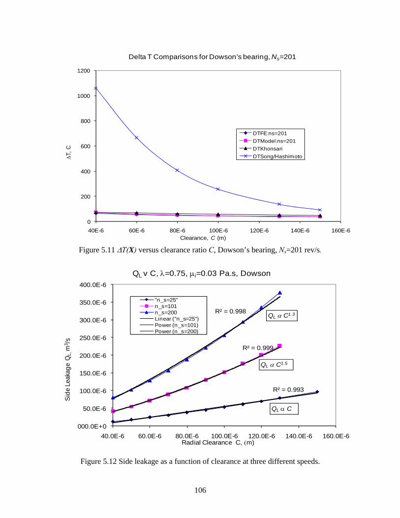
106
Figure 5.11 ΔT(X) versus clearance ratio C, Dowson’s bearing, Ns=201 rev/s.
Figure 5.12 Side leakage as a function of clearance at three different speeds.
0
200
400
600
800
1000
1200
40E-6 60E-6 80E-6 100E-6 120E-6 140E-6 160E-6
ΔT, C
Clearance, C (m)
Delta T Comparisons for Dowson's bearing, Ns=201
DTFE:ns=201DTModel:ns=201DTKhonsariDTSong/Hashimoto
R² = 0.993
R² = 0.999
R² = 0.998
000.0E+0
50.0E-6
100.0E-6
150.0E-6
200.0E-6
250.0E-6
300.0E-6
350.0E-6
400.0E-6
40.0E-6 60.0E-6 80.0E-6 100.0E-6 120.0E-6 140.0E-6 160.0E-6
Side
Lea
kage
QL,
m3 /s
Radial Clearance C, (m)
QL v C, λ=0.75, μi=0.03 Pa.s, Dowson
"n_s=25"n_s=101n_s=200Linear ("n_s=25")Power (n_s=101)Power (n_s=200)
QL α C
QL α C1.5
QL α C1.3

107
5.3.5 Temperature Increase ΔT, Side Leakage QL as Function of Diameter
The effect of varying diameter D while holding the length L constant for Dowson’s
bearing is analyzed. Figure 5.13 shows the temperature increase ΔT(X) while figure 5.14
shows leakage variation. Figure 5.13 is plotted by holding the length of Dowson’s
bearing constant and varying the diameter. Song’s model is included for completeness of
the discussion although it is clearly unsuitable for the range of bearings tested. Their
model is based on the friction force which is calculated by considering the local Reynolds
number (Re=ρCU/μ). There appears to be no method of updating the viscosity for use in
computation of the Reynolds number in their model. The other models show steady rise
with increasing diameter although the gradient ∂ΔT/∂D increases in the region
0.1<D<1.25 after which it decreases.
Figure 5.13 ΔT(X) as a function of diameter D.
0
50
100
150
200
250
300
350
400
450
0.04 0.06 0.08 0.10 0.12 0.14 0.16 0.18 0.20
ΔT, C
Diameter D, (m)
Delta T vs D, Ns=101rps, Dowson
FE@101Model@101Khonsari@101Song/Hashi@101

108
Figure 5.14 QL as a function of diameter D, Dowson’s bearing, Ns=25 rev/s. The relation
is linear as expected at this speed.
5.3.6 Simulation Results with ΔT (f1) and QL (f2) as Objective Functions
The set of equations developed are used to minimize a multi-objective function of
temperature increase ΔT(X) (F1) and side leakage QL (F2) using the design variable set
( )μλ,,CX T = , (same set used by Hashimoto [34] and Song et al. [36] ). Hashimoto’s
model is for high speed (up to 240 rev/s) and short bearings (0.2<λ<0.6) whereas the
model developed here is for medium speed (up to 200 rev/s) and medium range
(0.4<λ<1.0). The two objective functions are combined using scaling and weighting
factors to form one multi-objective function, F(X)=α1β1ΔT+α2β2QL which is minimized
subject to linear and non-linear constraints given in equation 5.14(b) and (c). Additional
0.00E+00
1.00E-05
2.00E-05
3.00E-05
4.00E-05
5.00E-05
6.00E-05
7.00E-05
0.04 0.06 0.08 0.10 0.12 0.14 0.16 0.18 0.20
Leak
age
QL,
m3 /s
Diameter D, (m)
Leakage Flow Vs Diameter, Dowson's Data, C=80 mm
ModelKhonsariFESong/Hashimoto

109
input parameters for Dowson’s bearing to run the optimization model are given in table
D.5. Results will be compared to those obtained by Song et al. for high-speed, short
bearings where a similar objective function was used (included for comparison only as
input parameters are different).
Results from both the classical (SQP) and a hybrid method are compared and presented in
figures 5.15, 5.16, 5.17 and 5.18. At least three runs with many sub-iterations were
performed for each method. Figure 5.15 compares results of the objective function from
the two methods at load 10 kN. The hybrid algorithm needed at most two runs to produce
a consistent result. SPQ however required at least four runs while adjusting the initial
guess to get reasonable predictions. Comparison with Song’s results show a similar
pattern to the objective function although Song’s values are lower due to different input
parameters and range (see table D.5). Clearance ratio predictions from the model (figure
5.16(b)) show a rapid initial increase and leveling off at speeds above 80 rev/s. This is
different from Song’s model prediction (figure 5.16(a)), which shows an initial decline,
leveling off, and gradual increase at speeds greater than 120 rev/s. Actual values of C in
Song’s model are much lower than model predictions.
Length to diameter λ predictions are shown in figure 5.17(b) for the model and 5.17(a)
for Song’s model. Both show a decline to the lower bound of λ, the model showing a
faster descend than Song’s model. Thus a similar pattern is exhibited by both models.
Finally viscosity variation μ for both models show predictions in the lower bound values
as shown in figure 5.18 (a) and (b).
In summary, the following points are evident:
• Objective function predictions F(X) show a smooth increase for both models
110
• Clearance ratio requirements for wider bearings appear to be higher than
shorter bearings
• Length to diameter ratio λ decreases to the lower bound in both cases,
declining faster for wider bearings.
• Viscosity remains at the lower bound in both cases. Obviously viscosity
values should be as low as possible to minimize viscous dissipation.
The next section extends the design variable set to four ( ( )sT pCX ,,, μλ= ) by including
supply pressure variation; the optimization work primarily focuses on pressure fed
bearings. The multi-objective function is also reformulated by considering minimization
of the power loss PL and leakage QL ; these two are axiomatically independent [39].

111
(a)
Figure 5.15 (a) Objective function from Song et al. [36], and (b) F(X) predictions from
SQP and hybrid algorithm, Wd=10kN for both cases.
2
4
6
8
10
12
14
16
18
50 100 150 200 250
Objective Funcition
f(X)
Speed, rev/s
Objective Function: SQP vs GA
SQP
GeneticAlg
Objective Function f(X): SQP vs Hybrid
0
10
20
30
40
50
60
0 10 20 30 40 50 60 70 80 90 100 110 120 130 140 150 160 170 180 190 200
Speed, rps
f(X)
f(X): HybridSQP: 7 Attempts
W = 10 kN

112
(a)
(b)
Figure 5.16 (a) Clearance ratio C as a function of speed for Song’s model (b) Model predictions, Wd=20 kN
40
50
60
70
80
90
100
50 100 150 200 250
Radial Clearance
C, μm
Speed, rev/s
Radial Clearance, μm
SQP
GA
Radial Clearance C : SQP vs Hybrid
000E+0
50E-6
100E-6
150E-6
200E-6
250E-6
0 10 20 30 40 50 60 70 80 90 100 110 120 130 140 150 160 170 180 190 200 210
Speed, rps
Rad
ial C
lear
ance
C,
m
C: SQPC: Hybrid
W = 10 kN

113
(a)
Figure 5.17 (a) Length to diameter ratio λ as function of speed, Song’s model, and (b)
Length to diameter ratio λ as function of speed for SQP and hybrid algorithm for developed model.
0.10
0.15
0.20
0.25
0.30
50 100 150 200 250
Length to
Diameter λ
Speed, rev/s
Length to Diameter Variation λ
SQP
GA
Length to Diameter Ratio λ Comparisons
0
0.2
0.4
0.6
0.8
1
1.2
0 10 20 30 40 50 60 70 80 90 100 110 120 130 140 150 160 170 180 190 200
Speed, rps
λ
1:SQP: 7 attemps
2: Hybrid
W = 10 kN

114
(a)
(b)
Figure 5.18(a) Viscosity variation, Song/Hashimoto’s model [36] (b) Viscosity variation
versus speed, hybrid and SQP.
0.900.920.940.960.981.001.021.041.061.081.10
50 100 150 200 250
Viscosity
μ, P
a.s
Speed, rev/s
Viscosity Variation μ
SQP
GA
Viscosity μ Comparisons
0.006
0.009
0.012
0.015
0.018
0.021
0.024
0.027
0.03
0.033
0 10 20 30 40 50 60 70 80 90 100 110 120 130 140 150 160 170 180 190 200
Speed, rps
Viso
cosi
ty μ
, (Pa
.s)
2: Hybrid
SQP: 7 Attempts
W = 10 kN

115
5.4 Power Loss PL (F1) and Leakage QL (F2) as Objective Functions
5.4.1 Power Loss Predictions from Model
Power loss comparisons for the proposed model, Jang and Khonsari’s [55], finite
element, and Hashimoto/Song’s models [34,36] is shown in figure 5.19 for Dowson’s
bearing [59]. Five measured data points and standard error bars are included; these show
the consistently better prediction from the model. Figure 5.20 presents simulation results
for Costa’s data [69]. Both figures show the relative accuracy of the proposed model for
the range of bearings tested (0.4<λ<1.5 and 0<Ns<200 rev/s). Model predictions are well
within the 95% confidence level. Another advantage is the ease with which the model can
be implemented. Equation set 5.9 computes the coefficient of friction f, friction force F,
and power loss PL.
Figure 5.19 Power loss prediction – Dowson’s data.
0100200300400500600700800900
100011001200130014001500160017001800
5 7 9 11 13 15 17 19 21 23 25 27 29 31 33 35 37 39 41 43 45 47 49 51
Pow
er L
oss,
W
Speed, rev/s
Power Loss Comparisons - Dowson's Data
Exp. PointsFEModelKhonsariSong/Hashimoto
Exp. DataSpeed, rps Power Loss, W11.7 153.113.3 189.216.7 280.820.8 406.425 532

116
Figure 5.20 Power loss predictions – Costa’s data.
5.4.2 Determination of weighting parameters and scaling factors
The method of weighting/scaling factors is used to determine optimum values for the
design variables. Input data shown in Tables D.1 and D.5 is used. Values of leakage QL
were weighted appropriately by using a suitable value for β2 while the scaling factors
were selected after comparing the absolute values of the objective function F(X) as a
function of the ratio α1/α2. Three values of the ratio were tried, namely 5, 1, and 1/5. It is
assumed the objective functions f1 and f2 are of equal importance and this means the
magnitude of the two should be equal or nearly so. The effect of weighting factor β2 of
105 is to transform leakage values, which are in the order 10-5 m3/s to the same order of
magnitude as power loss. Values of f1 and f2 are adjusted to be of equal magnitude by
0
500
1000
1500
2000
2500
3000
3500
4000
4500
5000
5500
6000
6500
7000
7500
8000
8500
9000
0 10 20 30 40 50 60 70 80 90 100 110 120 130 140 150 160 170 180 190 200 210
Pow
er L
oss,
W
Speed, rev/s
Power Loss Comparisons, Costa Bearing, 70 kPa
Exp. PointFEModelKhonsariSong/Hashimoto
Measured DataPowerLossns=33rps=612 WPowerLossns=50rps=1125 WPowerLossns=67rps=1663 W

117
selecting α1/α2=1/5, β1=1/400, β2=105 as shown in figure 5.22a. It is important that
values of the objective functions be similar if they are of equal importance (somewhat
like ‘comparing oranges with oranges’). It must be emphasized that the ultimate choice of
the weighting parameters depends on the relative importance of each objective function f1
and f2 [34]. These graphs show that power loss f1 increases more rapidly than leakage f2
thus having a greater influence on the objective function value F(X). Depending on the
relative importance of minimizing the power loss or leakage, figure 5.21 gives an
indication on what route to take. An assumption is made here that the goal is to obtain the
lowest possible value of the objective function and use α1/α2=1/5.
The effect of scaling factors β1 and β2 with α1/α2=1/5 is shown in figures 5.22, 5.23 and
5.24. Also included are the values of F1, F2 and the design variable sets (C,λ,μ,ps). One
observation is increasing clearance ratio reduces power loss but increases side leakage
significantly. Figure 5.21 shows results with β1=1/400 and β2=105 which has the effect
reducing power loss contribution to F(X). The net result is minimizing side leakage has
more weight and clearance ratio is at the minimum value in 5.21c while length to
diameter ratio λ is at the upper limit of 1. Supply pressure predictions show rapid
increase with increasing speed to the upper limit at a speed of 40 rev/s. Viscosity is
virtually at the minimum allowable in all cases. The trends change significantly
however, when β1 is increased to 1/35 in figure 5.22, making minimization of power loss
(F1) more important (figure 5.22a). Supply pressure increases rapidly to the upper limit as
before, however higher clearance ratio values are predicted. Length to diameter values
shift lower while viscosity remains at the lower values. Significant changes occur with
β1=1 (figure 5.23) as supply pressure increases less rapidly, viscosity remains at the

118
lower limit, clearance ratio is initially high and reduces, while length to diameter ratio λ
reduces further to values in the region of 0.65 at higher speeds.
Figure 5.21 f(X) as function of α1/α2, scaling parameters: β1=1, β2=105
Objective Function Values for Different Scaling Factors
0
500
1000
1500
2000
2500
3000
0 20 40 60 80 100 120 140 160 180 200
Speed, rps
Obj
. Fun
ctio
n f(x
)
α1/α2=5
α1/α2=1
α1/α2=1/5

119
(a)
(b)
(c)
(d)
(e)
Figure 5.22 Model predictions with α1/α2=1/5, β1=1/400, β2=105
Objective function F(X), F 1 , F 2 for β 1 =1/400
0
5
10
15
20
25
30
0 20 40 60 80 100 120 140 160 180 200
Speed, rps
Obj
ectiv
e fu
nctio
n f (X)f_1f_2
000E+050E+3
100E+3150E+3200E+3250E+3300E+3350E+3400E+3
0 20 40 60 80 100 120 140 160 180 200
p s, k
Pa
Speed, rps
Supply pressure ps variation
p_s
Variation of clearance ratio C
30E-6
32E-6
34E-6
36E-6
38E-6
40E-6
42E-6
0 20 40 60 80 100 120 140 160 180 200Speed, rps
Rad
ial C
lear
ance
C,
mC
Viscosity variation μ
0.000
0.005
0.010
0.0150.020
0.025
0.030
0.035
0 20 40 60 80 100 120 140 160 180 200
Speed, rps
Visc
osity
μ,
(Pa.
s)
μ
Length to diameter ratio λ
0.9
1
1.1
0 20 40 60 80 100 120 140 160 180 200Speed, rps
λ
λ

120
(a)
(b) (c)
(d)
(e)
Figure 5.23 Model predictions with α1/α2=1/5, β1=1/35, β2=105
Objective function F(X) , F 1 and F 2
0
20
40
60
80
100
120
140
0 20 40 60 80 100 120 140 160 180 200
Speed, rps
Obj
ectiv
e fu
nctio
n f
f(X)
f_1
f_2
Variation of supply pressure p s
0
50
100
150
200
250
300
350
400
0 20 40 60 80 100 120 140 160 180 200Speed, rps
Supp
ly p
ress
. ps
, kPa
p_s
Variation of clearance ratio C
39E-640E-641E-642E-643E-644E-645E-646E-647E-648E-6
0 20 40 60 80 100 120 140 160 180 200Speed, rps
Rad
ial C
lear
ance
C,
m
C
Variation of inlet viscosity μ
0
0.002
0.004
0.006
0.008
0.01
0.012
0 20 40 60 80 100 120 140 160 180 200
Speed, rps
Visc
osity
μ, (
Pa.s
)
μ
Variation of λ: Hybrid
0.8
0.85
0.9
0.95
1
1.05
0 20 40 60 80 100 120 140 160 180 200
Speed, rps
λ
λ

121
(a)
(b) (c)
(d)
(e)
Figure 5.24 Model predictions with α1/α2=1/5, β1=1, β2=105
Objective functions F(X), F 1, F 2
0500
10001500200025003000350040004500
0 20 40 60 80 100 120 140 160 180 200
Speed, rps
Obj
. fun
ctio
n
f (X)f_1f_2
050
100150200250300350400
0 20 40 60 80 100 120 140 160 180 200
p s, k
Pa
Speed, rps
Variation of supply pressure ps
p_s
4.0E-054.5E-055.0E-055.5E-056.0E-056.5E-057.0E-057.5E-058.0E-058.5E-05
0 20 40 60 80 100 120 140 160 180 200
C, m
Speed, rps
Variation of clearance ratio C
C
Variation of inlet viscosity μ
0
0.002
0.004
0.006
0.008
0.01
0.012
0 20 40 60 80 100 120 140 160 180 200
Speed, rps
Visc
osity
μ, (
Pa.s
)
μ
Length to diameter ratio λ
0.4
0.5
0.6
0.7
0.8
0.9
1
0 20 40 60 80 100 120 140 160 180 200
Speed, rps
λ
λ

122
5.4.3 Pareto Optimal Front Method
The method of Pareto diagrams eliminates the need for scaling and weighting factors
[40,42]. Pareto fronts for a load of W=10 kN are developed. The two objective functions
are plotted on the axes and a series of non-inferior points plotted. These charts can be
very effective in helping designers choose design variable sets depending on the relative
importance they place on each objective function. Pareto optimal fronts at common
speeds for these bearings (1500 rev/min (25 rev/s), 2000 (33.3), 3000 (50) and 4000
(66.7)) are shown in figures 5.25 and 5.26. Included in each chart is a boxed value for the
recommended operating point. The design variable set for this point is also shown. The
power loss range is small in these plots because the Pareto fronts are developed by
changing the supply pressure and determine its effect on both objective functions. The
Pareto optimal fronts all satisfy the condition in equation 5.12. The Pareto table at 4000
rpm is shown in Table 5.6.

123
(a)
(b)
Figure 5.25 Pareto optimal front for speeds of (a)1500 rpm and (b) 2000 rpm.
Pareto Optimal Front, N s =25 rps
25.70E-6
25.80E-6
25.90E-6
26.00E-6
26.10E-6
26.20E-6
26.30E-6
26.40E-6
26.50E-6
26.60E-6
26.70E-6
418.5 419 419.5 420 420.5
Power Loss, W
Leak
age
m3 /s 6.94E-5,0.734,0.01,75E3
Pareto Optimal Front, Ns=33.3 rps
30.60E-6
30.80E-6
31.00E-6
31.20E-6
31.40E-6
31.60E-6
31.80E-6
583.6 584.1 584.6
Power Loss, W
Leak
age,
m3 /s
65.2E-6,0.697,0.01,107E3

124
(a)
(b)
Figure 5.26 Pareto optimal front for (a) 3000 rpm and (b) 4000 rpm. Power loss in Watts.
Pareto Optimal Front, N=50 rps
41.80E-6
41.90E-6
42.00E-6
42.10E-6
42.20E-6
42.30E-6
42.40E-6
931.7 931.85 932 932.15 932.3 932.45
Power Loss, W
Leak
age,
m3 /s
6.11E-5,0.664,0.01,184E3
Pareto Optimal Front, Ns=66.7 rps
53.20E-6
53.30E-6
53.40E-6
53.50E-6
53.60E-6
53.70E-6
53.80E-6
53.90E-6
54.00E-6
54.10E-6
54.20E-6
1257.3 1257.45 1257.6 1257.75 1257.9 1258.05Power Loss, W
Leak
age,
m3 /s
59.9E-6,0.652,0.01,250E3

125
Table 5.6 Typical Pareto Table for Bearing at 4000 rpm, W=10kN
Power Loss
PL, Watts
Leakage
QL (m3/s)
Clearance
C (μm)
Length to
Diameter
ratio λ
Supply
pressure ps
1257.354 54.138E-6 60.050 0.65197 140.0E+3 1257.354 54.051E-6 60.051 0.65205 150.0E+3 1257.381 53.950E-6 60.031 0.65201 160.0E+3 1257.419 53.801E-6 60.002 0.65203 179.1E+3 1257.420 53.796E-6 60.002 0.65203 180.0E+3 1257.470 53.670E-6 59.965 0.65200 200.0E+3 1257.540 53.546E-6 59.913 0.65195 225.0E+3 1257.560 53.516E-6 59.898 0.65192 235.0E+3 1257.607 53.464E-6 59.864 0.65188 250.0E+3 1257.652 53.421E-6 59.830 0.65182 260.0E+3 1257.687 53.394E-6 59.805 0.65178 270.0E+3 1257.721 53.371E-6 59.780 0.65173 279.5E+3 1257.776 53.339E-6 59.740 0.65166 293.9E+3 1257.815 53.323E-6 59.711 0.65162 305.0E+3 1257.877 53.298E-6 59.666 0.65151 320.0E+3 1257.916 53.288E-6 59.638 0.65146 330.0E+3
5.5 Extended Optimization Model
5.5.1 Leakage Flow Equation and Validation
The flow equation presented by Zengeya and Gadala [76] and detailed in section 5.3
assumes flow is a function of aspect ratio L/D and eccentricity ratio ε, (QL=f(λ,ε)) only; it
does not explicitly consider the effect of supply pressure and oil groove geometry on
leakage flow rate. The method proposed by Martin [70] considers leakage flow as the sum
of a hydrodynamic pressure-induced and velocity-induced components. The drawback of
Martin’s work is in the many considerations of bearing inlet conditions (oil hole/oil
groove, film thickness at inlet port hg, and parameter fg which is a function of the oil
groove or hole dimensions). This justifies the need for formulating a simplified leakage
flow model with less complex considerations while maintaining accurate predictions. The

126
work presented by Zengeya and Gadala [76] is used as a base and expanded here to take
the effect of groove geometry Lg/L, groove location θ, groove length to diameter ratio
Lg/D into account, i.e., ⎟⎟⎠
⎞⎜⎜⎝
⎛=
LL
DL
pFQ ggsL ,,,,, θλε . Based on extensive numerical
simulations using the streamline upwind Petrov-Galerkin finite element method, the
following equation for leakage flow rate is proposed:
( )( ) ( )[ ]ελθ ln05.15.02.0exp15.13.0117.016.11 5.1 +−⎟⎟⎠
⎞⎜⎜⎝
⎛⎟⎟⎠
⎞⎜⎜⎝
⎛+++=
LL
DL
pQ ggsL (5.16)
where sp , the non-dimensional supply pressure 2
2⎟⎠⎞
⎜⎝⎛=
RC
Np
ps
ss πμ
is determined using
the fluid pressure ps, the fluid viscosity μ, the journal speed Ns (rev/s), and the radial
clearance C. Other parameters in equation 5.16 include the length to diameter ratio λ =
L/D, the groove length Lg, and the groove location θ. It should be noted that θ can be
positive or negative as shown in figure 4.1a; it varies between ±π/2. The exponential part
of the equation is adopted from the work of reference 76. Depending on the nature of the
bearing set-up, appropriate terms in equation 5.16 may be ignored.
Justification for the choice/form of sp and θ (linear) in equations 5.16 follows. Figures
5.27 to 5.31 show the linear relationship between leakage flow and supply pressure,
groove location and eccentricity ratio for some bearing data. Figure 5.27a illustrates the
effect of supply pressure on flow rate for Claro’s data [79] at eccentricity ε=0.7, speed
Ns=8.6 rev/s and supply pressure variation from 8 to 60 kPa. Maximum error of 17 per
cent from experimental data is better than 25 per cent reported in Claro’s work
(error=(predicted-experimental)/experimental value)x100). Standard error bars also

127
reveal two data points outside the 95% confidence level. Figure 5.27b shows model
predictions on Costa’s data [69] at speed Ns=50 rev/s, eccentricity ε=0.5 and supply
pressure values ranging from 70 to 300 kPa. Maximum error is 19 per cent with two
points outside the 95% confidence level. Figure 5.28 presents flow as a function of speed
at two supply pressures for Dowson’s data [80,81]. Predictions from the model show a
maximum error of 14 per cent while Dowson’s is 21. Both models fall outside the 95%
confidence level for the experimental data at ps=170kPa. Figure 5.29 shows the effect of
both supply pressure and eccentricity ratio on leakage flow for Dowson [80] whose
model predictions are included for comparison. Both models are accurate at zero
pressure; however the model developed here shows better prediction of the data as
indicated by determining the variance of each in table 5.7. The goodness of fit, however,
is poor at 1.0. The accuracy of the model at two supply pressures is tested in figure
5.30 while figure 5.31 presents non-dimensional leakage flow as a function of
eccentricity ratio from Boncompain [15] and Ferron [75]. Two other predictions are
included for comparison. Error bars in figure 31a indicate all models fail to accurately
predict higher eccentricity values.

128
(a)
(b)
Figure 5.27 (a) Leakage flow prediction and data as a function of supply pressure for Claro’s data [79]. Groove at +90° to the load line. Other bearing parameters as in Table
D2. (b) Data from Costa et al. [69]. Groove location: +30°
0
0.1
0.2
0.3
0.4
0.5
0.6
0 10 20 30 40 50 60 70
Non
-dim
. leak
age
Supply pressure, kPa
Measured vs Predicted Leakage, Claro et al., θ=+90o
Measured
Model
LQ
0
0.1
0.2
0.3
0.4
0.5
0.6
0.7
0 0.05 0.1 0.15 0.2
Non
-dim
. leak
age
Non-dim supply presure
Predicted vs Measure values, Costa ( =0.03,0.04,0.09,0.13,0.19 kPa, θ=+30)
Model
Measured
LQ
sp
sp

129
Figure 5.28 Leakage flow as function of supply pressure, Costa [69]. Ns=50 rpm, ε=0.5.
Figure 5.29 Non-dimensional leakage flow as a function of eccentricity ratio for Boncompain [15] and Ferron [75].
0.00E+00
5.00E-06
1.00E-05
1.50E-05
2.00E-05
2.50E-05
0 5 10 15 20
Leak
age
flow
QL,
m3 /s
Speed, rev/s
Predicted, Measured, and Dowson Leakage Data
Measured:ps=170kPaQ_LDowson:ps=170kPaQMeasured:ps=0Q_LModel:ps=0Q_LDowson:ps=0Q_LModel:ps=170kPaQ_LKhonsari:ps=0Q_LKhonsari:ps=170kPa
0.00
0.20
0.40
0.60
0.80
1.00
1.20
1.40
0.15 0.25 0.35 0.45 0.55 0.65 0.75 0.85
Non-
dim
ensi
onal
flow
Eccentricity ratio ε
Non-dimensional Flow: Predicted vs Measured Values
Measured:ps=0Qmodel:ps=0Measured@ps=0.5Qmodel:ps=0.5Mesured@ps=1Qmodel:ps=1Dowson:ps=0Dowson:ps=0.5Dowson:ps=1

130
Table 5.7 Comparison of variance between model and Dowson’s predictions.
Variance
Model Dowson0 0.0022 0.0015
0.5 0.0065 0.01571.0 0.0121 0.0176
Figure 5.30 Leakage flow as a function of speed ps=0 and 170 kPa, Dowson’s [80].
Leakage Flow Vs Speed, Dowson/Taylor
0.0E+00
1.0E-05
2.0E-05
3.0E-05
4.0E-05
5.0E-05
6.0E-05
0 20 40 60 80 100 120 140 160 180 200
Speed, rps
Leak
age
flow
, m3 /s
ps170ps=0
Model predictions (measured data in brackets)ps=0: QL,ns=13.3=5.4x10⁻⁶ (5.2x10⁻⁶) m3/sps=170kPa: QL,ns=13.3=22.1x10⁻⁶(21x10-6) m3/s
sp

131
(a)
(b)
(c)
(d)
Figure 5.31 Non-dimensional leakage flow LQ as a function of eccentricity ratio for Boncompain [15] and 75 [75].
5.5.2 Power Loss Equation and Validation
Power loss determination follows a similar procedure presented in section 5.4. The
coefficient of friction parameter (R/C)f in reference 76 is expanded to include effects of
0
0.2
0.4
0.6
0.8
1
1.2
0.30 0.40 0.50 0.60 0.70 0.80 0.90
Non
-dim
ensi
onal
flow
Eccentricity ε
Leakage Flow vs Eccentricty, 1500 rpm
MeasuredMartinKhonsariModel
LQ
0.0
0.2
0.4
0.6
0.8
1.0
0.15 0.25 0.35 0.45 0.55 0.65 0.75 0.85
No
n-d
imen
sio
nal f
low
Eccentricity ε
Leakage Flow vs Eccentricity, 2000 rpm
modelkhonsariMartinMeasured
LQ
0
0.1
0.2
0.3
0.4
0.5
0.6
0.7
0.8
0.9
0.30 0.40 0.50 0.60 0.70 0.80
Non
-dim
ensi
onal
flo
w
Eccentricity ε
Leakage Flow vs Eccentricity, 3000 rpm
modelExp. Datakhonsarimartin
LQ
0.0
0.1
0.2
0.3
0.4
0.5
0.6
0.7
0.8
0.20 0.30 0.40 0.50 0.60 0.70
Non
-dim
ensi
onal
flow
Eccentricity ε
Leakage Flow vs Eccentricity, 4000 rpm
modelkhonsarimartinExp. data
LQ
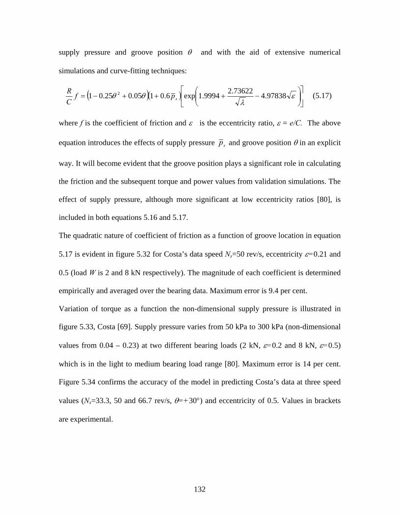
132
supply pressure and groove position θ and with the aid of extensive numerical
simulations and curve-fitting techniques:
( )( ) ⎥⎦
⎤⎢⎣
⎡⎟⎟⎠
⎞⎜⎜⎝
⎛−+++−= ε
λθθ 97838.473622.29994.1exp6.0105.025.01 2
spfCR (5.17)
where f is the coefficient of friction and ε is the eccentricity ratio, ε = e/C. The above
equation introduces the effects of supply pressure sp and groove position θ in an explicit
way. It will become evident that the groove position plays a significant role in calculating
the friction and the subsequent torque and power values from validation simulations. The
effect of supply pressure, although more significant at low eccentricity ratios [80], is
included in both equations 5.16 and 5.17.
The quadratic nature of coefficient of friction as a function of groove location in equation
5.17 is evident in figure 5.32 for Costa’s data speed Ns=50 rev/s, eccentricity ε=0.21 and
0.5 (load W is 2 and 8 kN respectively). The magnitude of each coefficient is determined
empirically and averaged over the bearing data. Maximum error is 9.4 per cent.
Variation of torque as a function the non-dimensional supply pressure is illustrated in
figure 5.33, Costa [69]. Supply pressure varies from 50 kPa to 300 kPa (non-dimensional
values from 0.04 – 0.23) at two different bearing loads (2 kN, ε=0.2 and 8 kN, ε=0.5)
which is in the light to medium bearing load range [80]. Maximum error is 14 per cent.
Figure 5.34 confirms the accuracy of the model in predicting Costa’s data at three speed
values (Ns=33.3, 50 and 66.7 rev/s, θ=+30°) and eccentricity of 0.5. Values in brackets
are experimental.

133
Figure 5.32 Torque predictions as a function of groove position, Costa [69]. Supply
pressure of 70 kPa.
Figure 5.33 Torque predictions as a function of non-dimensional supply pressure, Costa
et al. [69].
2.00
2.50
3.00
3.50
4.00
4.50
-0.6 -0.5 -0.4 -0.3 -0.2 -0.1 0 0.1 0.2 0.3 0.4 0.5 0.6
Torq
ue, N
.m
Groove position, radians
Predicted Vs Measured Torque: ps=70kPa
TvTheta:Model_W=2kN
Measured@2kN
TvTheta:Mode_W=8kN
Measured@8kN
DataMeasured at 2kN: 2.7 N.mPredicted at 2kN: 2.9 N.m (9.4%)Measured at 8kN: 3.7 N.mPredicted at 8kN: 4.0 N.m (6.8%)
0.00
0.50
1.00
1.50
2.00
2.50
3.00
3.50
4.00
0 0.05 0.1 0.15 0.2 0.25
Torq
ue, N
.m
Non-dimensional supply pressure
Predicted vs measured torque values, θ=-30o
Model@2kNMeasured@2kNModel@8kNMeasured@8kN
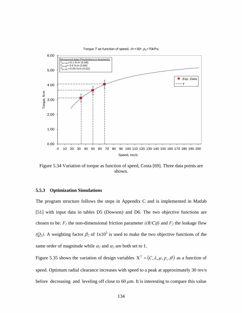
134
Figure 5.34 Variation of torque as function of speed, Costa [69]. Three data points are shown.
5.5.3 Optimization Simulations
The program structure follows the steps in Appendix C and is implemented in Matlab
[51] with input data in tables D5 (Dowson) and D6. The two objective functions are
chosen to be: F1 the non-dimensional friction parameter ((R/C)f) and F2 the leakage flow
(QL). A weighting factor β2 of 1x10⁵ is used to make the two objective functions of the
same order of magnitude while α1 and α2 are both set to 1.
Figure 5.35 shows the variation of design variables ( )θμλ ,,,,XTspC= as a function of
speed. Optimum radial clearance increases with speed to a peak at approximately 30 rev/s
before decreasing and leveling off close to 60 μm. It is interesting to compare this value
0.00
1.00
2.00
3.00
4.00
5.00
6.00
0 10 20 30 40 50 60 70 80 90 100 110 120 130 140 150 160 170 180 190 200
Torq
ue, N
.m
Speed, rev/s
Torque T as function of speed, θ=+30o, ps=70kPa
Exp. Data
T
Measured data (Predictions in brackets):TNs=33.3=3.1 N.m (3.08)TNs=50= 3.6 N.m (3.66)TNs=66.7=4.05 N.m (4.02)

135
(a) (b)
(c)
(d)
(e)
Figure 5.35 Variation of XT as a function of speed, W=10kN. Model predictions with α1/α2=1, β1=1, β2=105
Optimum radial clearance C
0.0E+00
2.0E-05
4.0E-05
6.0E-05
8.0E-05
1.0E-04
1.2E-04
1.4E-04
0 20 40 60 80 100 120 140 160 180 200Speed, rps
Rad
ial c
lear
ance
C
C
Optimum L/D λ ratios
0.3
0.4
0.5
0.6
0.7
0.8
0.9
1
0 20 40 60 80 100 120 140 160 180 200
Speed, rpm
L/D
ratio
λ
λ
Optimum viscosity μ
0
0.005
0.01
0.015
0 20 40 60 80 100 120 140 160 180 200Speed, rps
Vis
cisi
ty, P
a.s
μ
Optimum supply pressure p_s
0
10
20
30
40
50
60
0 20 40 60 80 100 120 140 160 180 200
Speed, rps
Supp
ly p
ress
ure,
kPa
p_s
Optimum groove position θ
-1.8-1.6-1.4-1.2-1.0-0.8-0.6-0.4-0.20.0
0 20 40 60 80 100 120 140 160 180 200
Speed, rps
Gro
ove
posi
tion
θ
θ

136
with 138.8µm used by Dowson [80]. The predicted value is obtained with groove
position θ=-π/2. Their data shows bearing speeds up to 16.7 rev/s. Another interesting
observation is evident when figure 5.35a is compared to figure 11c in reference 76 where
the groove is positioned at the load line. The predicted peak clearance of 120 μm at 15
rev/s in figure 5.35a is significantly higher than a peak of 79 μm at 10 rev/s in figure 11c,
reference 76. Corresponding C values at each speed are generally higher in figure 5.35a,
suggesting optimum groove location allows for higher optimum clearance ratios.
Length to diameter ratio values (figure 5.35b) decrease from a high of 0.94 and levels off
at 0.67. This pattern is similar for both bearings simulated and is also comparable to
figure 11c, reference 76.
Optimum viscosity is at the lower bound as expected. This is because lower viscosity
lowers power loss as well as increases leakage for the same set of bearing input variables.
Similar findings are reported by other researchers [34,36].
Supply pressure is predicted to be at the lower bound for all speeds. This is significantly
different from predictions in figure 11b, reference 76 where it increases from the lower to
upper bounds. Groove location appears to have a significant effect on supply pressure.
Lower values can be used when optimum location is used in journal bearing design.
Groove location prediction is interesting in that the model indicates optimum placing of
the groove at the lower bound (-π/2), figure 5.35e. Although this position has the least
leakage flow, it has significant power loss minimization. Obviously no consideration of
whether this position is in the rupture zone and what effect that it has on mechanical
stresses is taken. For convenience most journal bearings are designed with groove

137
location in line with the load. The other potential beneficial position, although not shown
in the figures, is at the upper bound (+π/2) which gives slightly higher F(X) values.
Figure 5.36 shows variation of the design variables as a function of speed for a load of
W=700N. The results are similar to those in figure 5.35 although peak C value of 107
μm occurs at higher speed (25 rev/s). Length to diameter ratio levels off at a lower value
of 0.45 in figure 5.36b compared to 0.67 in figure 5.35b.
Pareto charts present an alternative method of showing optimum design points. A typical
pareto optimal front for load W=10kN and speed 50 rev/s is shown in figure 5.37a. In
figure 5.37b the load is 700N and speed 25 rev/s. Two finite element predictions with the
boxed XT values are included, showing the accuracy of the optimization model. The
graph shows significant power loss variation. Pareto charts present a set of non-
dominated solutions, thus each point on the front has its own merits. A wide range of
these charts can be produced at small speed increments. Designers can then make use of
these charts in design decisions. An interesting observation is in the power loss values
predicted in figure 5.37a (740W) compared to figure 13a (932W), reference 76 for
similar input values. Significant power loss savings can be realized with proper groove
location.

138
(a) (b)
(c) (d)
(e)
Figure 5.36 Variation of XT as a function of speed, load W=700N.
Optim um radial clearance C as function of speed
0.0E+00
2.0E-05
4.0E-05
6.0E-05
8.0E-05
1.0E-04
1.2E-04
0 20 40 60 80 100 120 140 160 180 200
Speed, rps
Rad
ial c
lear
ance
C,
m
C
Variation of L/D ratio λ
0.0
0.1
0.2
0.3
0.4
0.5
0.6
0.7
0.8
0.9
1.0
0 20 40 60 80 100 120 140 160 180 200
Speed, rps
λ
λ
Optimum viscosity μ as function of speed
0
0.002
0.004
0.006
0.008
0.01
0.012
0 20 40 60 80 100 120 140 160 180 200
Speed, rps
Visc
osity
, Pa.
s
μ
Optim um supply pressure ps
0
10
20
30
40
50
60
0 20 40 60 80 100 120 140 160 180 200
Speed, rps
Sup
ply
pres
sure
. kP
a
ps
Optimum groove location θ
-1.8
-1.6
-1.4
-1.2
-1.0
-0.8
-0.6
-0.4
-0.2
0.00 20 40 60 80 100 120 140 160 180 200
Speed, rps
Gro
ove
loca
tion,
radi
ans
θ

139
(a)
(b)
Figure 5.37(a) Pareto optimal front for speeds of 1500 rpm, W=10kN; (b) Pareto optimal
front, W=700N
Pareto front, W= 10kN, N s =50 rev/s
3.00E-05
3.10E-05
3.20E-05
3.30E-05
3.40E-05
3.50E-05
3.60E-05
3.70E-05
710 720 730 740 750 760 770 780Power Loss, W
Leak
age
flow
, m3 /s
PfrontFE
63.3e-6,0.818,01,50e3,-1.571
68.1e-6,0.699,01,50e3,-1.571
Pareto Chart, Speed=1500 rpm, Load=700N
0.0E+00
2.0E-06
4.0E-06
6.0E-06
8.0E-06
1.0E-05
1.2E-05
35 45 55 65 75 85Power Loss, W
Leak
age
Flow
, m3 /s
Ns=1500rpmFE
1.16e-4,0.728,01,50e3,-1.571
4.72e-5,0.47,01,50e3,-1.571

140
5.6 Interpretation of Optimization Results
A brief overview of the optimization results is appropriate here. Results from the four
variable model are analyzed in more detail and compared to five variable ones.
5.6.1 Pareto Optimal Fronts with X , , , and X , , , ,
The Pareto charts in figure 5.25 show a variation of power PL and leakage flow QL of
less than one and four percent respectively. The power loss variation is small, and in
engineering terms might be interpreted to mean other factors have more influence in
determining bearing performance. Noting that for this set the load is in line with the oil
groove, it is clear this position limits the extent to which power loss and side leakage can
be influenced.
The situation is however significantly different when groove location θ is included in the
design set. As shown figure 5.37a power loss variation is 8% while leakage flow varies
23% which gives a significant influence on the two performance parameters. Table 5.7
summarizes the results from the two sets. Further analysis of the results appear in
reference 76.
Table 5.8 Variation of Performance Parameters PL and QL
Characteristic Variation % X , , , Power Loss 0.2
Leakage flow 1 X , , , , Power Loss 8
Leakage flow 23

141
5.6.2 Uncertainty in the Results
The optimization model is based on fundamental engineering principles of lubrication
flow and temperature increase as proposed by the respected research teams Jang and
Khonsari [55] and Khonsari et al. [74]. There is no reason to doubt the validity of the
temperature rise parameters in reference 76 or the form of the flow equation in reference
76. What might be questioned is the accuracy of the data used. Dowson’s data [59] is
regarded as a benchmark in lubrication circles while Costa et al. [69] present a wide
variety of performance data which is also well taken in the industry. Unfortunately both
sets of researchers do not present any error analysis with their data.
The finite element simulations presented in earlier chapters (and Appendix E) were
shown to be accurate in predicting experimental data from Boncompain [15], Ferron [75],
Costa [69] and others [72,73,79,80,81]. Prediction results were compared to available
models and shown to be at least as good or better [73].
5.7 Chapter Summary
An Empirically Derived Optimization Model (EDOM) is proposed for length to diameter
ratio 0.4≤λ≤1.0. Both minimization of the temperature increase ΔT and leakage QL as
well as power loss PL and leakage QL are analyzed. The objective function minimizing
power loss PL and side flow QL is preferable as it minimizes two independent functions.
The proposed approach can be used by design engineers who need simple and effective
models to help them choose optimum design variables using readily available
optimization programs such as Matlab’s Optimization Toolbox. Such an approach
presents advantages over more complex methods such as Hirani’s model in that no
complex integration techniques are required.

142
Model predictions for temperature increase, leakage flow, and power loss are accurate in
comparison to models in the literature. The equations are empirically derived and make
the need for complex integrations unnecessary.
The method of weighting functions/scaling parameters as well as Pareto optimal fronts
are used. The benefits of each method are assessed. Pareto optimal diagrams eliminate
the need to determine the weights and scaling required in the first method and should be
used more often in journal bearing design.
The model is extended to include groove position and supply pressure computations
explicitly by introducing terms width to diameter ratio (wg/D) and groove length to
bearing length ratio (Lg/L). Maximum error of 15% on leakage is observed from the
proposed model. The model is comprehensive yet simple to implement, and depending
on the nature of the problem some terms in the equations may be ignored. Power loss
and torque predictions are within 10% of experimental data. These results show the
effectiveness of the model and the ease of use in bearing optimization problems.
Model results show that groove location has a significant effect on the optimization of the
bearing. The model predicts groove location should be at the lower bound (-π/2). Higher
values of clearance ratio C may be used when optimum groove position is chosen.
Significant power loss savings may be realized with appropriate location of oil groove.
143
Chapter 6
Summary, Conclusions and Future Work
6.1 Summary and Conclusions
Journal bearing design and optimization requires accurate and reliable prediction of
thermal fields due to viscous dissipation. The effect of temperature increase on load
carrying capacity of the bearing can be dramatic due to a decrease in the viscosity of the
film.
Several thermo-hydrodynamic (THD) models in the literature focus on formulating a
robust, rapid converging THD model that can be used in optimization where many
iterations at varying speeds are required. This requirement presents one of the main
challenges for researchers and is the focus of this work. A robust and effective FEA
procedure is proposed and a novel and simple model for journal bearing is introduced.
Applications of the developed models to the analysis and optimization of practical cases
are discussed. Main outcomes from the work are summarized in the following.
1. Rapid Thermal Predictions: Streamline Upwind Petrov-Galerkin FE Method
The first goal was to formulate a THD model in a robust, efficient and as general as
possible form. The streamline upwind Petrov-Galerkin finite element (SUPG-FE) method
for three dimensional THD lubrication modeling is developed using Cartesian
coordinates. It is shown to be effective in slider as well as journal bearings with some
minor modifications. In summary the streamline upwind Petrov-Galerkin FE method can
be effectively used to model journal bearings using Cartesian coordinates. The model can
be refined, especially the boundary conditions in the groove area, to give more accurate

144
results. The same model can also be used for slider bearings with less implementation
requirements. A more detailed model procedure is given in sections 2.4 and 3.3.
2. Slider Bearing Thermal Predictions
Some important observations on slider bearings are noted. An aspect ratio between 2 and
1 is ideal in terms of leakage flow and minimum peak temperatures. A unique way of
identifying this region is illustrated where the differential of the flow Q∂ as a function of
aspect ratio )/( BL
Q∂
∂ reduces rapidly to minimum before increasing again and becoming
constant at BL / ratios higher than 10. The above findings along with the flow gradient
method (FGM), uniquely defined in this work, helps optimize slider bearing tilt ratio for
minimum temperature rise.
3. Development of Journal Bearing Template
A template for modeling THD lubrication in journal bearings is shown to be effective in
modeling thermal effects, leakage flow, and cavitation effects. The model as presented
has no special consideration of thermal boundary conditions at the rupture interface.
Although the approach proposed by Boncompain [15] is used in the rupture zone, focus
on the dynamics of velocity gradients ∂v/∂y and ∂w/∂y near the rupture and reformation
interfaces are critically analyzed and appear to explain the rapid decline in temperature.
Thermal predictions are within ten percent of measured values. The model is robust and
converges in two or three iterations making it ideal for iterative applications such as in
validating optimization equations developed in the second part of the research.
4. Empirically Derived Optimization Model (EDOM)
A novel set of optimization equations derived from first principles is proposed. The set of
equations require no complex integrations and can be easily implemented using standard

145
optimization tools such as Matlab. Optimization equations for temperature increase ΔT,
power loss PL, and leakage flow QL are developed; constants and other values in the
equations are determined empirically for the range of bearings under consideration. The
set of equations are well-designed and easy to use while giving accurate results.
Comparisons with models in literature show that the equations consistently give better
predictions.
The approach used by Jang and Khonsari [55] whereby temperature rise parameters are
derived and empirically verified is expanded on and used to formulate temperature
increase ΔT(X) model. Such an approach is used for the first time in journal bearing
optimization. It presents an alternative to Hirani and Suh’s model [38] which requires a
finite difference mass conserving algorithm to determine temperature increase and
integration techniques to determine leakage flow and power loss.
Once empirical values in the temperature increase ΔT(X), leakage QL, and power loss PL
are determined, the optimization model can be used for the range of bearings under
consideration to find optimum values of the design variables (X). This work presents the
developed equations as an optimization model.
5. Optimization using Weight/Scaling Parameters and Pareto Optimal Fronts
The developed set of equations are used to minimize a multiobjective function
optimization model using the weight/scaling factors and Pareto optimal fronts and results
are compared to Hashimoto’s [34]. It is clear Hashimoto’s model is for short bearings
with L/D ratios up to 0.5 and is not accurate for medium range bearings (0.4<L/D<1.0)
under consideration here.
In the Pareto optimal front approach, posterior articulation of the weights is used whereby
the designer initially generates a number of non-inferior (a set of equally efficient)

146
solutions from which a final decision is made on any one solution. Advantages and
disadvantages of each method are given, however Pareto charts appear to be preferable as
they give a set of non-inferior, non-dominated solutions and final choice depends on the
merits of a particular design.
6.2 Recommendations for Future Work
1. Journal Bearing Template
The developed SUPG FE model, although effective in predicting thermal effects, should
be extended to thermo-elastohydrodynamic (TEHD) lubrication where expansion of the
shaft and bush are taken into account. This will give a better prediction of the load
carrying capacity of the bearing. Prediction of the clearance ratio C could be adjusted
accordingly.
The journal bearing template developed here could be tested on transient phenomenon
such as the squeeze effect and thermal predictions during start-up and shut down. This is
an important area as it is also linked to the study of bearing time to seizure and how this
can be avoided.
2. Journal Bearing System Optimum Design
The model presented here focuses on individual journal bearings. A possible expansion
of the work might involve looking at the ‘system’ of a shaft and two journal bearings at
the end. Such a task would the overcome the qualifying statement in section 4.3.5 that
other factors may influence the choice of design variable set (X) such as the shaft
stiffness and misalignment problems that may be encountered.
147
3. Expansion of the Empirically Derived Optimization Model
The optimization model developed here works well for medium range journal bearings.
An extension of the model could be developed for short and long range bearings. This
would be very useful to design engineers who use bearings in the two ranges and also
make the EDOM applicable to the full range of aspect ratios.

148
Bibliography
1. Khonsari, M.M., Wang, S.H., “Note on transient thermo-hydrodynamic lubrication
effects in lubricating films”, STLE Tribol. Trans., 35, pp. 177-183, 1992.
2. Pinkus, O., Thermal Aspects of fluid film tribology, ASME Press, New York, 1990.
3. Ettles, C.M.M., Cameron, A., “Considerations of oil flow across a bearing groove”,
Trans. ASME J. Lub. Tech., pp. 312-319, 1968.
4. Ettles, C.M.M., “Solutions for flow in a bearing groove”, Proc. Instn. Mech. Engrs.,
182, p.120, 1967-8.
5. Kosasih, P.B., Tieu, A.K., “An investigation into the thermal mixing in journal
bearings”, Proc. Inst. Mech. Engrs. Part J: J. Eng. Tribol., 218, pp. 379-389, 2004.
6. Costa, I., Miranda, A.S., Fillon, M., Claro, J.C.P., “An analysis of the influence of oil
supply conditions on the thermo-hydrodynamic performance of a single-groove
journal bearing”, Proc. Inst. Mech. Engrs. Part J: J. Eng. Tribol., 217 (J2), pp. 133-
144, 2003.
7. Rodkiewicz, C.M., Sinha, P., “On the lubrication theory: a mechanism responsible for
generation of the parallel bearing load capacity”, Trans. ASME J. Tribol., 105, pp.
584-590, 1993.
8. Schumack, M.R., “Application of the pseudo-spectral method to thermo-
hydrodynamic lubrication”, Int. J. Numer. Methods. Fluids, 23, pp. 1145-1161, 1996.
9. Ratish Kumar, B.V., Srinivasa Rao, P., Sinha, P., “A SUPG/FEM analysis of thermal
effects on load carrying capacity in slider bearing lubrication”, Numer. Heat Transfer
Part A, 38(3), pp. 305-328, 2000.
149
10. Ratish Kumar, B.V., Srinivasa Rao, P., Sinha, P., “A numerical study of performance
of a slider bearing with heat conduction to pad”, Fin. Elem. Analysis Design, 37, pp.
533-547, 2001.
11. Brooks, A.N., Hughes, T.J.R., “Streamline upwind/Petrov-Garlerkin formulations for
convective dominated flows with particular emphasis on the incompressible Navier-
Stokes equations”, Comp. Methods Appl. Mech. Eng., 32, pp. 199-259, 1982.
12. Grygiel, J-M., Tanguy, P.A., “Finite element solution for advection-dominated
thermal flows”, Comput. Methods Appl. Mech. Eng., 93(3), pp. 277-289, 1991.
13. Zengeya, M., Gadala, M., “Viscous dissipation effects in hydrodynamic lubrication”,
Proc. Zim. Inst. Engrs., 4(1) , pp. 5-16, 2006.
14. Ezzat, H.A., Rohde, S.M., “A study of the thermo-hydrodynamic performance of
finite slider bearings”, Trans. ASME J. Lub. Tech., 95(3), pp 298-307, 1973.
15. Boncompain, R., Fillon, M., Frene, J., “Analysis of thermal effects in hydrodynamic
bearings”, Trans. ASME J. Tribol., 108, pp. 219-224, 1986.
16. Gero, L.R., Ettles, C.M., “A three-dimensional thermo-hydrodynamic finite element
scheme for fluid film bearings”, ASLE Tribol. Trans., 31(2), pp 182-191, 1988.
17. Hahn, E.J., Kettleborough, C.F., “Solution for the pressure and temperature in an
infinite slider bearing of arbitrary profile”, Trans. ASME J. Lub. Tech., 89, p 445,
1967.
18. Kucinschi, B.R., Dewitt, K.J., Pascovici, M.D., “Thermoelastohydrodynamic (TEHD)
analysis of a grooved thrust bearing”, Trans. ASME J. Tribol., 126(2), pp. 267-274,
2004.

150
19. Paranjpe, R. S., Goenka, P.K., “Analysis of crankshaft bearings using a mass
conserving algorithm”, STLE Tribol. Trans., 33(3), pp 333-344, 1990.
20. Paranjpe, R.S., Han, T., “A finite volume analysis of the thermo-hydrodynamic
performance of finite journal bearings”, Trans. ASME J. Tribol., 112, pp 557-566,
1990.
21. Paranjpe, R.S., Han, T., “A study of the thermo-hydrodynamic performance of
steadily loaded journal bearings”, STLE Tribol. Trans., 37(4), pp 679-690, 1994.
22. Stachowiak, G.W., Batchelor, A.W., Engineering Tribology, 2nd Ed., Butterworth, p.
216, 2001.
23. Booker, J.F., Huebner, K.H., “Application of the finite element methods to
lubrication: an engineering approach”, Trans. ASME J. Lub. Tech., pp 313-323, 1972.
24. Goenka, P.K., “Dynamically loaded journal bearings: finite element method
analysis”, Trans. ASME J. Tribol., 106, pp 429-439, 1984.
25. Labouff, G.A., Booker, J.F., “Dynamically loaded journal bearings: a finite element
treatment for rigid and elastic surfaces”, Trans. ASME J. Tribol., 107(4), pp 505-515,
1985.
26. Bayada, G., Chambat, M., El Alaoui, “Variational formulations and finite element
algorithms for cavitation problems”, Trans. ASME J. Tribol., 112, pp 398-403, 1990.
27. Kucinschi, B-R., Fillon, M., Frene, J., Pascovici, M.D., “A transient
thermoelastohydrodynamic study of steadily loaded plain journal bearings using finite
element method analysis”, Trans. ASME J. Tribol., 122(1), pp 219-226, 2000.
28. Elrod, H.G., “A cavitation algorithm”, Trans. ASME J. Lub. Tech., 103(3), pp. 350-
354, 1981.

151
29. Kumar, A., Booker, J.F., “A finite element cavitation algorithm”, Trans. ASME J.
Tribol., 113, pp 276-286, 1991.
30. Kumar, A., Booker, J.F., “A mass and energy conserving finite element lubrication
algorithm”, Trans. ASME J. Tribol., 116, pp 667-671, 1994.
31. Optasanu, V., Bonneau, D., “Finite element mass-conserving cavitation algorithm in
pure squeeze motion”, Trans. ASME J. Tribol., 122, pp 162-169, 2000.
32. Colynuck, A.J., Medley, J.B., “Comparison of two finite difference methods for the
numerical analysis of thermo-hydrodynamic lubrication”, STLE Tribol. Trans., 32,
pp. 346-356, 1989.
33. Shigley, J.E., Mischke, C.R., Budynas, R.G., Mechanical Engineering Design, 7th
Ed., McGraw-Hill, New York, p. 619, 2004.
34. Hashimoto H., “Optimum design of high-speed, short journal bearings by
mathematical programming”, STLE Tribol. Trans., 40(2), pp. 283-293, 1997.
35. Hashimoto H., Matsumoto K., “Improvement of operating characteristics of high-
speed hydrodynamic journal bearings by optimum design: part I – Formulation of
methodology and its application to elliptical bearing design”, Trans. ASME J.
Tribol., 123, pp. 305-312, 2001.
36. Song J-D, Yang B-S, Choi B-G, Kim H-J, “Optimum design of short journal bearings
by enhanced life optimization algorithm”, Tribol. Int., 38, pp. 403-412, 2005.
37. Yang B-S., Lee Y-H., Choi B-K., Kim H-J., “Optimum design of short journal
bearings by artificial life algorithm”, Tribol. Int., 34, pp. 427-435, 2001.
38. Hirani H, Suh NP, “Journal bearing design using multiobjective genetic algorithm
and axiomatic design approaches”, Tribol. Int., 38, pp. 481-491, 2005.

152
39. Suh NP, “Axiomatic design: advances and applications”, Oxford University Press,
2001.
40. Hirani, H., “Multiobjective optimization of journal bearing using the pareto
optimality concept”, Proc. Inst. Mech. Engrs. Part J: J. Eng. Tribol., 218(4), pp.
323-336.
41. Hirani, H., “Multiobjective optimization of journal bearing using mass conserving
and genetic algorithms”, Proc. Inst. Mech. Engrs. Part J: J. Eng. Tribol., 219(3), pp.
235-248, 2005.
42. Deb K, Multiobjective optimization using evolutionary algorithms, John Wiley &
Sons, New York, 2001.
43. Hashimoto, H., “Optimization of oil flow rate and oil film temperature rise in high
speed hydrodynamic journal bearing”, in: Dowson D., editor, Tribology for energy
conservation, Amsterdam, Elsevier, pp. 205-210, 1998.
44. Powell, M.J.D., “A fast algorithm for non-linearly constrained optimization
calculations”, GA Watson Ed., Lecture Notes in Mathematics, Springer Verlag, 630,
1978.
45. Goldberg, D.E., “Genetic algorithm in search, optimization and machine learning”,
Addison Wesley Publishing Company, 1989.
46. Holland, J.H., “Adaptation in natural and artificial systems”, University of Michigan
Press, Michigan, 1975.
47. DeJong, K., “The analysis and behavior of genetic adaptive systems”, PhD
Dissertation, University of Michigan, Michigan, 1975.

153
48. Homaifar, A., Qi, C.X., Lai, S.H., “Constrained optimization via genetic algorithms,
simulations”, Engineering Optimization, 62, pp. 242-254, 1994.
49. Louis, S.J., Zhoo, F., and Zeng, X., “Flaw detection and configuration with genetic
algorithms”: in Evolutionary Algorithms in engineering applications, Springer-
Verlag, 1997.
50. Saruhan, H., “Design of a three-lobe journal bearing using a genetic algorithm”, J.
Naval Sci. Eng., 2(2), pp. 87-103, 2004.
51. Genetic Algorithm and Direct Search Toolbox User’s Guide for use with Matlab, The
Mathworks Inc. 2004.
52. Zengeya, M., Gadala, M., Segal, G., “Three-dimensional thermal field in slider
bearings”, Proc. World Tribology Congress III, Washington DC, p. 30, September
12-16 2005.
53. Zengeya, M., Gadala, M., Segal, G., “Three-Dimensional Modeling of Thermo-
hydrodynamic Lubrication in Slider Bearings Using Streamline Upwind Petrov-
Galerkin Method”, Num. Heat Transfer, Part A, 49(10), pp. 947-968, 2006.
54. Dowson, D., “A generalized Reynolds equation for fluid-film lubrication”, Int. J.
Mech. Sci., 4, pp 159-170, 1962.
55. Jang, J.Y., Khonsari, M.M., “Design of bearings on the basis of thermodrodynamic
analysis”, Proc. IMechE J. Eng. Trib., 218, pp 355-363, 2004.
56. Segal, G. (2003), Sepran Standard Problems, Ingenieursbureau SEPRA, Den Haag,
The Netherlands.
57. Ezzat, H.A., Rohde, S.M., “A study of the thermo-hydrodynamic performance of
finite slider bearings”, Trans. ASME J. Lub. Tech., 95(3), pp. 298-307, 1973.
154
58. Boncompain, R., Frene, J., “Thermo-hydrodynamic analysis of finite journal bearings
– static and dynamic characteristics”: in Proc. 6th Leeds-Lyon Symposium on
Tribology: Thermal Effects in Tribology, pp. 33-41, 1980.
59. Dowson, D., Hudson, J., Hunter, B., March, C.N., “An experimental investigation of
the thermal equilibrium of steadily loaded journal bearings”, Proc. IMechE. Eng., 181
(3B), pp 70-80, 1966.
60. Reddi, M.M., “Finite element solution of the incompressible lubrication problem”,
Trans. ASME J. Lub. Tech., 69, pp 524-531, 1969.
61. Hahn, E.J., Kettleborough, C.F., “Solution for the pressure and temperature in an
infinite slider bearing of arbitrary profile”, Trans. ASME J. Lub. Tech., 89, p. 445,
1967.
62. Ingenieursbureau SEPRA, Park Nabij 3, 2491 EG Den Haag, The Netherlands.
63. Zengeya, M., Gadala, M., Segal, G. (2007). Hydrodynamic and thermal behavior of
journal bearings using streamline upwind Petrov-Galerkin FEM, STLE Tribology
Trans., 50(2), 227-247.
64. Hamrock, B.J., “Fundamentals of fluid film lubrication”, 2nd Edition, Marcel Dekker,
New York, p168, 2004.
65. Lebeck, A.O., “Parallel sliding load support in the mixed friction regime”, Trans.
ASME J. Trib., 109, pp. 189-195, 1987b.
66. Arnell, R.D., Davies, P.B., Halling, J., and Whomes, T.L., Tribology, principles and
design applications, Springer-Verlag, New York, 1991.
67. Ezzat, H.A., Rohde, S.M., “A study of the thermo-hydrodynamic performance of
finite slider bearings”, Trans. ASME J. Lub. Tech., 95(3), pp 298-307, 1973.

155
68. Khonsari, M.M., Booser, E.R., Applied tribology: bearing design and lubrication,
John Wiley, New York, p 215, 2001.
69. Costa, L., Fillon, M., Miranda, A.S., Claro, J.C.P., “An experimental investigation of
the effect of groove location and supply pressure on the THD performance of a
steadily loaded journal bearing”, ASME J. Trib., 122, pp 127-132, 2000.
70. Martin, F.A., “Oil flow in plain steadily loaded journal bearings: realistic predictions
using rapid techniques”, Proc. IMechE J. Eng. Tribol., 212, 1998, 413-425.
71. Kelly, D.W., Nakazawa, S., Zienckiewicz, O.C., “A note on upwinding and
anisotropic balancing dissipation in finite element approximations to convective
diffusion problems”, Int. J. Num. Meth. Eng., 15, pp. 1705-1711, 1980.
72. J. Mitsui, “A study of thermo-hydrodynamic lubrication in a circular journal bearing”,
Tribol. Int., 20(6), 331-341, 1987.
73. Pierre, I., Fillon, M., “Influence of geometrical parameters and operating conditions
on the thermo-hydrodynamic behavior of plain journal bearings”, Proc. IMechE J.
Eng. Tribol., 214, 2000, 445-457.
74. Khonsari, M.M., Jang, J.Y., Fillon, M., “On the generalization of thermo-
hydrodynamic analysis for journal bearings”, Trans. ASME J. Trib., 118, pp. 571-579,
1996.
75. Ferron, J., Frene, J., Boncompain, R., “A study of the thermo-hydrodynamic
performance of a plain journal bearing: comparison between theory and
experiments”, Trans. ASME J. Lub. Tech., 105, 422-428, 1983.
76. Zengeya, M, Gadala, M., “Optimization of journal bearings using a hybrid scheme”,
IMechE Part J: J. Eng. Tribol., 221(5), 591-607, 2007.

156
77. Khonsari M. M., Booser E.R., "Parasitic Power Losses in Hydrodynamic Bearings".
Machinery Lubrication, March 2006.
78. Optimization Toolbox for use with Matlab, User’s Guide Version 2, The Mathworks
Inc., 2003.
79. Claro, J.C.P., and Miranda, A.A.S., “Analysis of hydrodynamic journal bearings
considering lubricant supply conditions”, IMechE Part C: J. Mech. Eng. Sci., 207,
93-101, 1993.
80. Dowson, D., Taylor, C.M., Miranda, A.A.S., “The prediction of liquid film journal
bearing performance with a consideration of lubricant film reformation Part 1:
theoretical results”, Proc. IMechE J. Eng. Trib., 199(C2), 95-102, 1985.
81. Dowson, D., Taylor, C.M., Miranda, A.A.S. “The prediction of liquid film journal
bearing performance with a consideration of lubricant film reformation Part 2:
experimental results”, Proc. IMechE J. Eng. Trib., 199(C2), 103-111, 1985.

157
APPENDICES
APPENDIX A
A.1 Velocity fields u, v, and w
The equilibrium condition for forces acting in the x-direction gives
0=⎟⎟⎠
⎞⎜⎜⎝
⎛∂∂
∂∂
−∂∂
yu
yxp μ (A-1)
where u is the velocity of the lubricant in the direction of sliding. The boundary
conditions are u=0 at y=h and u=U at y=0. For the one-dimension bearing considered
here the value of the lubricant flow is constant along the bearing assuming no side
leakage; this fact is used to calculate v. Algebraically this means that the lubricant
velocity across the film thickness is constant, that is ( ) 00
=∂∂ ∫hudyx . Equation A-1 can be
integrated in the y-direction to get v, the component of u in that direction .
∫ ∫ ++=y y
UdyAdyydxdpyu
0 02)(
μμ (A-2)
where A is given by
( )
∫∫ −⎟⎟
⎠
⎞⎜⎜⎝
⎛−
= h
h
dy
UdyydxdpA
0
20
μ
μ (A-3)
and U the slider velocity in m/s. Non-dimensional value becomes / . Similar
equilibrium condition for forces acting in the y-direction is
0=⎟⎟⎠
⎞⎜⎜⎝
⎛∂∂
∂∂
−∂∂
yw
yzp μ (A-4)
with boundary conditions w=0 at y=0 and w=0 at y=h. Equation A-4 is integrated with
respect to y to give
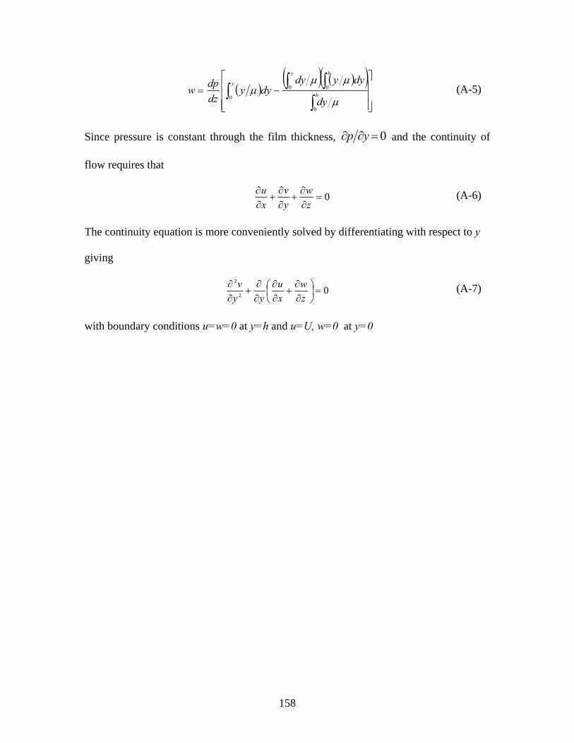
158
( )( ) ( )( )
⎥⎥⎥
⎦
⎤
⎢⎢⎢
⎣
⎡−= ∫
∫∫∫y
h
hy
dy
dyydydyy
dzdpw
0
0
00
μ
μμμ (A-5)
Since pressure is constant through the film thickness, 0=∂∂ yp and the continuity of
flow requires that
0=∂∂
+∂∂
+∂∂
zw
yv
xu (A-6)
The continuity equation is more conveniently solved by differentiating with respect to y
giving
02
2
=⎟⎠⎞
⎜⎝⎛
∂∂
+∂∂
∂∂
+∂∂
zw
xu
yyv (A-7)
with boundary conditions u=w=0 at y=h and u=U, w=0 at y=0

159
APPENDIX B
The term (1+εcosϕ)3 in equation 5.12, referred to as (hg/C)3 in Martin’s model, relates to
the case where the oil groove is line with the load. The same term applies for an inlet hole
of diameter DH in line with the load but fg in this case becomes
75.1
4.0675.0 ⎟⎠⎞
⎜⎝⎛ +=
LDf H
g 0.1<DH<0.25 (B.1)
and
'1'
,S
pSmtotL QQQ −= (B.2)
where S’=0.6.
Another important case is when the oil groove is at the maximum film thickness
position hmax where (hg/C)3 becomes
( )3
3
1 ε+=⎟⎟⎠
⎞⎜⎜⎝
⎛Chg (B.3)
equation B1 for fg is valid, and total leakage becomes
m
gmtotL L
LQQ ⎟⎟
⎠
⎞⎜⎜⎝
⎛=, 0.3<Lg/L<0.8 (B.4)
where 27.0
27.0 ⎟⎠⎞
⎜⎝⎛=
p
LQ
Qm . The proposed model here uses equation 10 to determine the
flow due to film pressure QL while Qp is evaluated using equation 13 with the appropriate
value of (hg/C)3.
The power value to eccentricity ratio in equation B4 applies when the hydrodynamic
film starts at hmax and L/D<1.0, 0.3≤λ≤0.9.

160
APPENDIX C
Optimization Procedure
The procedure presented here will help designers implement the optimization model
proposed. This can be easily done in Matlab.
A1. Sequential Quadratic Programming (SQP)
This requires three main components namely the main program, objective function, and
non-linear constraint m-files. The call to the optimization subroutine ‘fmincon’ is done in
the main program while computations in part B are done in the objective function m-file
and part C computes the non-linear constraints. Define global variables that will be
passed between the three m-files (ΔT, ε, Ns). The three m-files are attached at the end of
the appendix. While care was taken in preparing these files, no guarantee is given that the
codes are error free. A brief description of the main parts follows. Create a folder and
copy the three files. Run the main program which will call the other m-files.
Part A: Main Program
-Define upper and lower limits for design variable ( )sT pCX ,,, μλ= and provide
these as lb and ub in the call to ‘fmincon’
-Provide program with initial guess for design variable x0
-Set options and call ‘fmincon’ (this calls both Part B and C)

161
Part B: Objective Function
-Set all the problem parameters here (since the hybrid technique will use same
objective function)
For Ns from Ns1 to Ns max
Step 1: Compute journal surface velocity U
2: Use μI to compute Sommerfeld number S
3: Find eccentricity ratio ε
4: Compute the temperatures Tmax and Tshaft and temperature increase ΔT
5: Update the viscosity μ
6: Go to step 2 and re-compute S until convergence.
7: Compute the side leakage QL
8: Compute the objective function F(X) given the constraints gi(X)
9: Record F(X)
10. Loop and update Ns
Part C: Non-linear Constraint Computation
-Define minimum allowable hmin, ΔTa, ωcr ,and pa
-Compute pmax, ω, and ωcr
-Define non-linear constraints g1, g2, g3, and g4
C.2 Matlab M-files
Main Program function [X,FVAL,REASON,OUTPUT,POPULATION,SCORES] = dowprob1 %% This is an auto generated M file to do optimization with the Genetic Algorithm and % Direct Search Toolbox. Use GAOPTIMSET for default GA options structure.
%%Fitness function fitnessFunction = @dowtaylorobj; %%Number of Variables

162
nvars = 5 ; %Linear inequality constraints Aineq = []; Bineq = []; %Linear equality constraints Aeq = []; Beq = []; %Bounds LB = [4e-005 0.4 0.01 50000 -1.5708 ]; UB = [0.0003 1 0.03 350000 1.5708 ]; %Nonlinear constraints nonlconFunction = []; %Start with default options options = gaoptimset; %%Modify some parameters options = gaoptimset(options,'PopInitRange' ,[-2.5 ; 2.5 ]); options = gaoptimset(options,'PopulationSize' ,100); options = gaoptimset(options,'MutationFcn' , @mutationgaussian 1 1 ); options = gaoptimset(options,'Display' ,'off'); options = gaoptimset(options,'PlotFcns' , @gaplotbestf @gaplotbestindiv ); options = gaoptimset(options,'HybridFcn' , @fminsearch [] ); %%Run GA [X,FVAL,REASON,OUTPUT,POPULATION,SCORES] = ga(fitnessFunction,nvars,Aineq,Bineq,Aeq,Beq,LB,UB,nonlconFunction,options);
Objective Function
function [ret,f1,f2] = objective(x) global ns rho c_p D W e_0 deltaT Q_tot rfric1 p_max p_s f1 f2 a1 b1 c1 omega1 omega_cr tht_mn; global tht_mx p_smin p_smax; n_s = 3; % Journal speed, 40-240 rps n_smx =50; rho = 860; % Density of fluid, kg/m3 c_p = 2.0e3; % Specific heat of lubricant mu_i = 0.0358; % Inlet viscosity of oil, Pa.s T_i1 = 313; % Inlet oil temperature, K T_i = T_i1 - 273; % Inlet temp in C k_f = 0.13; % Thermal conductivity of lubricant, W/(m K) alpha = 0.756e-7; % Thermal diffusivity of lubricant, m^2/s beta = 0.0414; % Temperature-viscosity coefficient, K^(-1) L1 = 0.08; % Bearing length L_g1 = 0.07; % Length of groove L_Lg1 = L1/L_g1; % Ratio of groove/bearing length w_g = 12e-3; % Width of groove D = 0.1; % Journal diameter W = 20e3; % Load on bearing, N C_mn = 40.0e-6; % Radial clearance

163
C_mx = 300.0e-6; lambda_mn = 0.20; % L/D ratio lambda_mx = 1.0; mu_mn = 1.0e-3; % Viscosity mu_mx = 4.0e-2; p_smin = 50e3; % Supply pressure p_smax = 350e3;
beta1 = 1; % Scaling factor beta2 = 1e5; alpha1 = 1; % Weighting factor alpha2 =alpha1;
% Nonlinear objective function %x0 = [50e-6 0.6 2e-2];
for ns = n_s:n_smx, % Define the variables C=x(1); La=x(2); mu=x(3); p_s=x(4); theta = x(5); L = La*D; L_g = L_g1; R_C = D/(2*C); ps_bar = p_s*(1/R_C)^2/(mu*2*pi*ns); U = ns*2*pi*D/2; Re = rho*C*U/mu; S = ns*mu*D*L*(D/(2*C))^2/W; e_0 = -0.36667+0.49737/sqrt(La)-0.20986*log(S); if (e_0 > 1), e_0 = 0.6121; % return; end; % Compute side leakage Q_Leak Q_leak1 = exp(0.20-0.5*La^1.5+1.05*log(e_0)); Q_bar4 = (1+1.6*ps_bar)*(1+0.17*theta)*(1+0.3*w_g/D)*(1.15*L_g/L)*Q_leak1; Q_leak4 = Q_bar4*pi*ns*D*C*L; Q_leak = Q_leak1*pi*ns*D*C*L; % find leakage due to supply pressure z = 4*(1 + La*(1 - 1.25*e_0^0.18)); attit = atan((pi/(z*e_0))*sqrt(1-e_0^2)); f_g = (1.25-0.25*(L_g/L))/(3*(L/L_g-1)^(0.33333))+... (w_g/D)/(3*La*(1-L_g/L)); h_g = (1 + e_0*cos(attit))^3; Q_p =f_g*h_g*p_s*C^3/mu_i; % Leakage due to pressure Qm = Q_leak + Q_p - 0.3*sqrt(Q_leak*Q_p); % Datum flow rate S_prime = 0.7*(L_g/L)^0.7 + 0.4; Q_tot = Qm^S_prime*Q_p^(1-S_prime); % Total leakage %Compute temperature increase kappa1 = alpha*mu_i*beta*U*(D/(2*C))^2/(k_f*D/2); kappa2 = U*sqrt(mu_i*beta/k_f); % Determine parameters a, b, and c % if (e_0 > 0.1) && (e_0 < 0.3), % a1 = 1.58105; b1 = -0.14250; c1 = -1.04050; % end; if (e_0 >= 0.1) && (e_0 <= 0.7),

164
a1 = 1.5917; b1 = -0.13962; c1 = -1.24999; end; if (e_0 > 0.7) && (e_0 <= 0.9), a1 = 1.63973; b1 = -0.10627; c1 = -1.45216; end; % Compute T_max T_max1 = exp(a1 + b1/kappa1^0.5 + c1/kappa2^0.5); T_max = (T_max1/beta + T_i) + 273; deltaT = T_max - T_i1; % Compute Power loss rfrict = exp(1.9994+2.73622/sqrt(La)-4.97838*sqrt(e_0)); rfric1 = (1-0.25*theta^2+0.23*abs(theta))*(1+0.6*ps_bar)*(rfrict); torqueM = rfrict/R_C*W*D/2; torq2 = rfric1/R_C*W*D/2; P_Loss = torqueM*2*pi*ns; Ploss2 = torq2*2*pi*ns; % Recompute mu x(3) = mu_i*exp(-beta*deltaT); % Objective function f1 = alpha1*beta1*Ploss2; % Friction parameter obj function f2 = alpha2*beta2*Q_leak4; ret = f1 + f2;
end Non-linear Constraints M-file
function [c, ceq] = nonlin_cons(x) global ns rho c_p D W e_0 deltaT Q_tot rfric1 p_max p_s f1 f2 a1 b1 c1 omega1 omega_cr tht_mn; global tht_mx p_smin p_smax; h_a = 5e-6; % Allowable minimum film thickness p_a = 30e6; % Allowable maximum pressure, Pa deltaT_a = 70; % Allowable temperature rise, K p_max1 = exp(2.25062-0.39491/x(2)+4.77721*e_0^3); p_max = p_max1*x(3)*(D/2)^2*ns/x(1)^2 + p_s; omega1 = 2*pi*ns; omega_cr = sqrt(9.81/x(1))*(0.0584*exp(6.99*e_0^2.07)-1.318*e_0+2.873); g7 = h_a -x(1)*(1-e_0); g8 = deltaT - deltaT_a; %g9 = omega1 - omega_cr; g10 = p_max - p_a; c = [g7 g8 g10]; % nonlinear equality constraints returned as vector ceq ceq = []; % there are no nonlinear equality % constraints in

165
C3. Hybrid Scheme
The genetic algorithm toolbox with the Hybrid option was used. The fitness function is
the objective function defined in section C1 and non-linear constraints are the same as in
C1. Other settings are as shown in Table D5.

166
APPENDIX D
Tables
Table D.1 Input data from Dowson [59] and Song [36] bearings (empty cells mean unspecified values).
Input Parameter Dowson Song
Bearing Diameter D, m 0.102 0.1 Bearing width W, m 0.07625 -
Bush outer diameter, m 0.2 - Journal Speed (Ns=25rev/s), U 8.01 m/s -
Load, W 11000 10000 L/D 0.76 -
Radial clearance ratio R/C 800 - Groove width 4.76 x 10⁻³ m - Groove length 0.067 m -
Specific heat cf, cb, cs 2000, 380, 490 4190 Conductivities kf, kb, ks 0.13, 50, 65 W/m K -
Convective heat transfer coefficient H1, W/m2.K
100 -
Film/bush heat transfer coefficient H2, W/m2.K
200 -
Inlet temperature Ti 308 K - Inlet lubricant density ρi 867 kg/m3 -
Inlet viscosity μi 0.03 Pa.s - Viscosity-temperature coeff.
β 0.0414 /K -
Density-temperature coeff. δ
0.0012 /K -
Thermal diffusivity (αt=ρcp/kf)
0.756 x 10⁻⁷ m2/s -
Supply pressure ps (gauge) 0.276 x 10⁶ Pa -
D1.1 Location of thermocouples
Figure D1 shows the location of thermocouples (TC) on the bush and shaft in Dowson’s
experimental setup [59]. The temperature of the lubricant at inlet was recorded by two
iron-constantan thermocouples fitted in a radial inlet hole located within the bush. One of
the thermocouples was located near the outer radius of the bush while the other was

167
within 1.59 mm of the entry to the oil groove. Four outlet temperature thermocouples
were fitted in special oil scoops located at the ends of the bush to collect lubricant flow
leaving the bearing.
For bush temperature measurements, the thermocouples were mounted in groups of four
on bronze plugs which fitted closely into 34 radial holes in the bush. The hot junction of
each TC was located on the centerline of each plug and spaced at distances of 1.59, 17.5,
33.3, and 49.2 mm from the dead end of the radial hole adjacent to the oil film. The
bronze plugs were located in four planes at the axial locations shown in figure D1a.
Shaft temperatures were measured using twelve TC’s mounted in plugs similar to the
bush setup. The TC plugs were tightly fitted into radial holes in the shaft with their outer
ends flush with the shaft surface. The TC’s were located in four planes disposed about the
edge of the bearing as shown in figure D1b to enable temperature gradients to be
determined. Wires from the thermocouples ran along a hole drilled in the shaft to a slip-
ring assembly that was maintained at a constant temperature by air cooling at the end of
the shaft. The shaft surface temperature was recorded by means of a specially constructed
thin film platinum resistance thermometer mounted on a glass rod located in a radial hole
in the shaft at a distance of 16 mm from the central plane of the bearing. The exposed
surface of the glass plug was contoured to conform with the shaft surface. The leads fro
the platinum film were carried down the internal bore of the shaft to the slip ring
assembly.

Fiigure D1. Thhermocouplee location for
168
r pressure an
nd temperatuure measurem
ments [59]

169
Table D.2 Input values for the bearing tested by Boncompain et al. [15]
Input Parameter Value
Bearing Radius R, m 0.050 Bearing width W, m 0.08
Bush outer radius R2, m 0.100 Journal Speed (Ns=33.3rev/s), U 10.5 m/s
Eccentricity, ε 0.8 Radial clearance at 20°C, C, m-3 145µm
Groove angle 18° Groove length 0.070 m
Groove Location 0° Specific heats cf, cb, cs 2000, 380, 490
Conductivities kf, kb, ks, kg, W/m K
0.13, 250, 50, 0.025
Convective heat transfer coefficient , bush/ambient H1,
W/m2.K
100
Convective heat transfer coefficient , bush/oil and
shaft/oil interfaces H2, W/m2.K
500
Inlet temperature Ti, K 313 Ambient Temperature To, K 318
Inlet lubricant density ρi 860 kg/m3 Inlet viscosity μi 0.028 Pa.s
Viscosity-temperature coeff. β 0.0414 /K Density-temperature coeff. δ 0.0012 /K Supply pressure ps (gauge) 0.070 x 10⁶ Pa
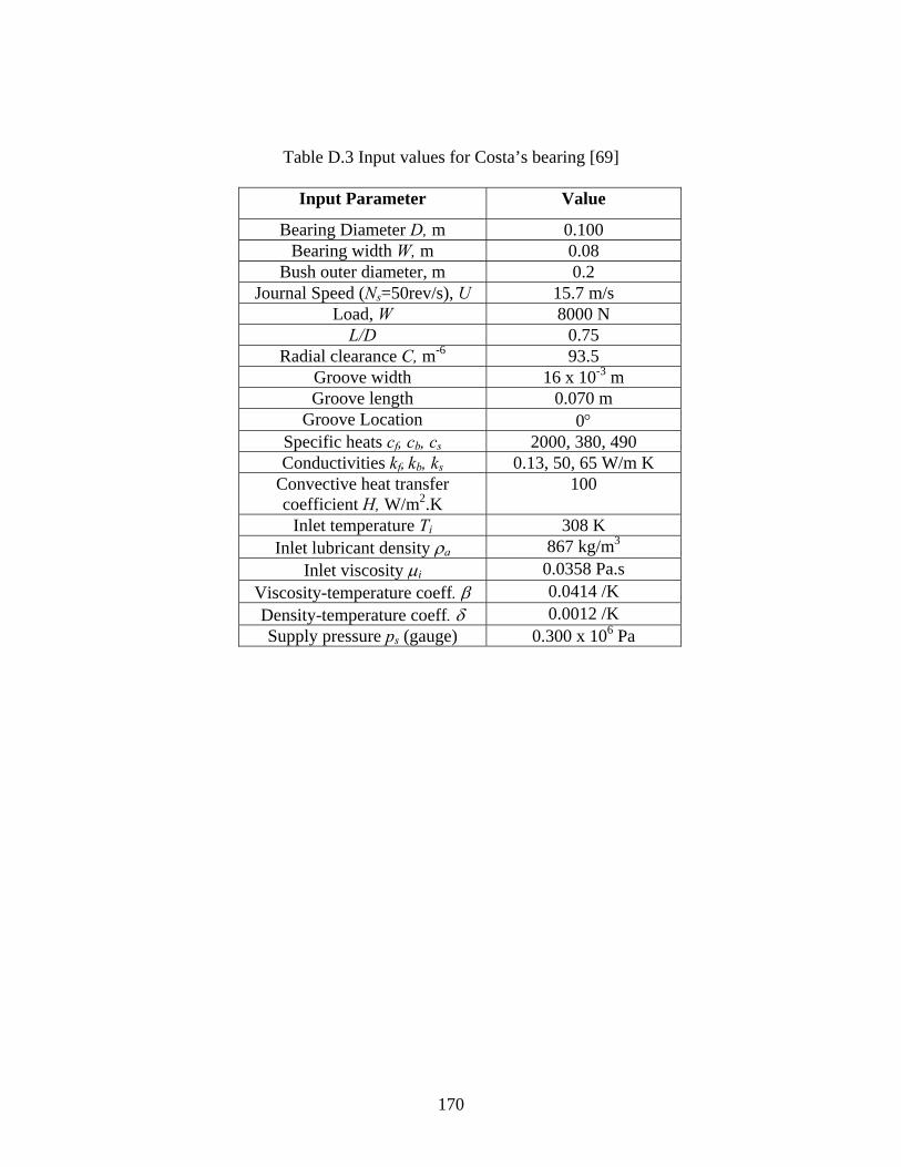
170
Table D.3 Input values for Costa’s bearing [69]
Input Parameter Value
Bearing Diameter D, m 0.100 Bearing width W, m 0.08
Bush outer diameter, m 0.2 Journal Speed (Ns=50rev/s), U 15.7 m/s
Load, W 8000 N L/D 0.75
Radial clearance C, m-6 93.5 Groove width 16 x 10-3 m Groove length 0.070 m
Groove Location 0° Specific heats cf, cb, cs 2000, 380, 490 Conductivities kf, kb, ks 0.13, 50, 65 W/m K
Convective heat transfer coefficient H, W/m2.K
100
Inlet temperature Ti 308 K Inlet lubricant density ρa 867 kg/m3
Inlet viscosity μi 0.0358 Pa.s Viscosity-temperature coeff. β 0.0414 /K Density-temperature coeff. δ 0.0012 /K Supply pressure ps (gauge) 0.300 x 10⁶ Pa

171
Table D.4 Input values for Ferron’s [75] bearing.
Input Parameter Ferron
Bearing Radius R, m 0.05 Bearing width L, m 0.08
Bush outer radius R2(assumed), m 0.1 Radial clearance at 20°C, C, m-6 145
Groove angle, ° - Groove length, m-3 70 (assumed) Groove Location, ° 0
Specific heats cf, cb, cs 2000, 380, 490 Conductivities kf, kb, ks, kg,
W/m K 0.13, 250, 50,
0.025 Convective heat transfer
coefficient , bush/ambient H1, W/m2.K
80
Convective heat transfer coefficient , bush/oil and shaft/oil
interfaces H2, W/m2.K
250
Inlet temperature Ti, K 313 Ambient Temperature To, K 313
Inlet lubricant density ρI, kg/m3 860 Inlet viscosity μi, Pa.s 0.0277
Viscosity-temperature coeff. β, /°K 0.0414 Supply pressure ps (gauge), kPa 70

172
Table D.5 Additional input data to run optimization simulations.
Parameter Dowson Song Minimum radial
clearance Cmin=40μm Cmin=40μm
Maximum radial clearance
Cmax=300μm Cmax=300μm
Minimum length to diameter ratio λ
λmin=0.4 λmin=0.2
Maximum length to diameter ratio λ
λmax=1.0 λmax=0.6
Minimum lubricant viscosity, Pa.s
μmin=0.01 μmin=0.001
Maximum lubricant viscosity, Pa.s
μmax=0.03 μmax=0.01
Minimum allowable film thickness
hmin=10 μm hmin=10 μm
Maximum allowable film pressure
pmax=10 MPa pmax=10 MPa
Allowable temperature rise
ΔTa=70 °C ΔTa=70 °C
Scaling (normalizing) factor
β1=1, β2=105 β1=1, β2=105
Weighting factor α1=1, α2=α1/5 α1=1, α2=α1/5 Load, kN 10, 20 10, 20
Population Size (Hybrid Technique)
100 20
Population Type Double Vector Initial Search Range -2.5 to 2.5
Fitness Scaling Rank Selection Function Stochastic Uniform
Reproduction: Cross-over Fraction
0.8
Mutation Function Gaussian Cross-over Function Scattered Migration Direction Forward

173
Table D6 Input data for Dowson [80] and Claro [79] bearings
Input Parameter Dowson et al. Claro
Bearing diameter D, m 0.0635 0.05 Bearing width L, m 0.0635 0.05 Radial clearance at 20°C, C, μm
138.8
125 Groove length Lg, m 0.026 0.04 Groove width wg, m 12x10-3 10x10-3 Groove Location, ° 0 +90° Specific heats cf, cb, cs 2000, (840), (490) (2000, 380, 490) Conductivities kf, kb, ks, kg, W/m K 0.13, (1.05), 50,
0.025 0.13, 250, 50,
0.025 Inlet temperature Ti, K 313 313 Ambient Temperature To, K (298) (298) Inlet lubricant density ρI, kg/m3
867.5
860 Inlet viscosity μi, Pa.s 0.0224 0.075 Viscosity-temperature coeff. β, /°K
(0.0414)
(0.0414) Supply pressure ps (gauge), kPa
0,170
8-60 Load W, N 700 824

174
APPENDIX E
Verification Examples
E1 Introduction
This section presents some further validation examples of the streamline upwind Petrov-
Galerkin finite element method developed. The classical method is compared to the
Galerkin and SUPG methods, namely the classical upwind scheme defined in section 2.5,
the doubly asymptotic, and discontinuity capturing methods. Brief definitions of each
follow.
E1.1 Upwinding Methods
If in the energy equation 2.11 the convective part u · dominates the diffusive part
, an improvement of the accuracy may be possible by applying the upwinding
method. It should be noted that upwinding does not always improve the accuracy and
moreover is more computationally expensive in building the matrices. The SUPG method
used in this work is based on the method proposed by Brooks and Hughes [11].
Essentially the method introduces an extra term to the standard Galerkin equation
Ω (E.1)
where e is the element, DT is the differential equation (energy equation in this case), f the
source term, and the weighting function that contains two parts, the Galerkin weighting
function and ζ defined in equation 2.30. The parameter defining the type of upwinding ξ
in equation 2.30 defines the type of upwinding. For the definition of ζ we introduce
η=uTΛu where Λ is the matrix with elements Λij and ν u ∆η
. The type of upwinding
becomes

175
1. Classical SUPG upwinding: ζ=1 which is used in all the results in thesis.
2. Doubly asymptotic approximation: ξν 3≤ν≤3
ν |ν|>3
3. Discontinuity capturing type 1 from Hughes et al. [11] where a pseudo velocity
u u· c where c is the degree of freedom (solution to be computed) is defined
and the upwind basis function ζ=(τ1u+τ2u )· where ∇Ni is the divergence of
the basis functions and ∆ and ∆ . For this case ξ is chosen
according to the doubly asymptotic approximation. (E.2)
More upwinding schemes appear in the work of Brooks and Hughes [11], however only
these three will be analyzed and results compared to the Galerkin method. The first
example analyses a convection-diffusion problem while the second compares SUPG and
Galerkin on lubrication data.
E.1.2 Convection Skew to the Mesh
E.1.2.1 Problem Statement
Consider a convection-diffusion problem defined by the general equation
u· (E.3)
where D is the diffusivity and c is the concentration of a molecular species. We assume
steady state conditions (∂c/∂t=0) and no source term (fs=0). We consider the flow in the
square shown in figure E1 with diffusivity D=10-6 with unidirectional and constant flow
u 1 (convection dominates the flow) .
Boundary conditions:
Lower boundary (y=0): Dirichlet (c=1)

176
Left boundary (x=0): Dirichlet (c=1 for y≤0.2 and c=0 for y>0.2)
Natural boundary condition, 0 imposed on all other boundaries
Flow Conditions:
The flow is unidirectional and constant ( u 1)
The angle of the flow α is an input variable chosen to be 45°.
Figure E1. Region for skew convection
Exact Solution:
The exact solution is equal to one in the region starting with lower boundary
condition c=1 and following a straight line with the angle of flow. Obviously the
value of c lies between o and 1 (0≤c≤1)
E.1.2.2 Solution Procedure
The diffusivity D is much less than flow velocity u thus the problem is convection-
dominated. The behavior of the standard Galerkin and the three upwind methods is
compared. Linear triangular elements are used. Figure E2 shows the mesh.
0.2 c=1
c=0
c=1 x
y
1
1
α
0 0

177
Figure E2. Mesh for convection-diffusion problem
E.1.2.4 Simulation Results
Appearance of wiggles in the solution is evident in the minimum and maximum values.
Table E1 compares results from the four methods.
Table E1. Minimum and maximum values of the solution
Method Minimum Maximum Galerkin -1.83421E-04 1.33327
SUPG first order -3.78362E-02 1.17226 SUPG double asymptotic -3.78362E-02 1.17226
SUPG discontinuity capturing -8.77571E-04 1.05377
The Galerkin method has the highest over-prediction in Table E1. Wiggles are most
apparent with the method as show in figure E3a. The discontinuity capturing SUPG
method (figure E3d) exhibits the least amount of wiggles although it is the most
expensive in terms of computing time and effort.

178
(a)
(b)
(c)
(d)
Figure E3. Three-dimensional plots of solutions from (a) Galerkin, (b) first order SUPG,
(c) double asymptotic SUPG, and (d) discontinuity capturing SUPG
E.1.3 SUPG/Galerkin Comparison on Journal Bearings
Experimental data from Costa et al. [69] and Dowson [59] are simulated using the three
methods. An estimate of the error is determined from
(E.4)
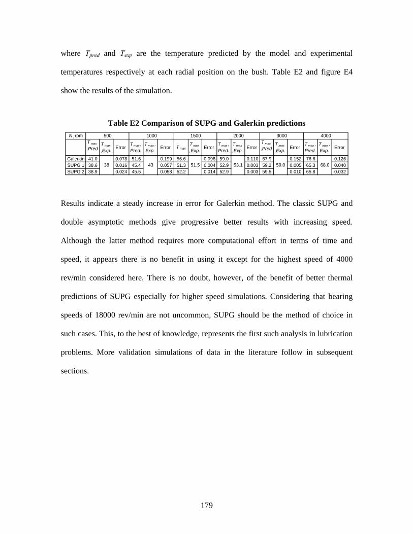
179
where Tpred and Texp are the temperature predicted by the model and experimental
temperatures respectively at each radial position on the bush. Table E2 and figure E4
show the results of the simulation.
Table E2 Comparison of SUPG and Galerkin predictions N , rpm
T max
,PredT max
,Exp.Error
T max ,Pred.
T max ,Exp.
Error T maxT max
,Exp.Error
T max ,Pred.
T max
,Exp.Error
T max
,PredT max
,Exp.Error
T max ,Pred.
T max ,Exp.
Error
Galerkin 41.0 0.078 51.6 0.199 56.6 0.098 59.0 0.110 67.9 0.152 76.6 0.126SUPG 1 38.6 0.016 45.4 0.057 51.3 0.004 52.9 0.003 59.2 0.005 65.3 0.040SUPG 2 38.9 0.024 45.5 0.058 52.2 0.014 52.9 0.003 59.5 0.010 65.8 0.032
38
500
53.1 59.051.5
1500 3000 4000
43 68.0
1000 2000
Results indicate a steady increase in error for Galerkin method. The classic SUPG and
double asymptotic methods give progressive better results with increasing speed.
Although the latter method requires more computational effort in terms of time and
speed, it appears there is no benefit in using it except for the highest speed of 4000
rev/min considered here. There is no doubt, however, of the benefit of better thermal
predictions of SUPG especially for higher speed simulations. Considering that bearing
speeds of 18000 rev/min are not uncommon, SUPG should be the method of choice in
such cases. This, to the best of knowledge, represents the first such analysis in lubrication
problems. More validation simulations of data in the literature follow in subsequent
sections.

180
Figure E4 SUPG and Galerkin predictions as a function of speed
E2 Slider bearing simulation
This example is from Arnell [66] (example 5.4.3, page 136) and analyzes three slider
bearings using the infinitely long approximations (ILA) for maximum pressure pm, flow
rate Qi, load capacity Wd, and frictional power loss PL. This example is from Arnell [66]
(example 5.4.3, page 136) and analyzes three slider bearings using the infinitely long
approximations (ILA) for maximum pressure pm, flow rate Qi, load capacity Wd, and
frictional power loss PL.
E2.1 Problem Statement
A thrust bearing of length L=0.2 m and width B=0.05 m operates with a minimum film
thickness of 0.0001m and sliding velocity U=3 m/s, effective viscosity is µ=0.04 Pa.s,
30
35
40
45
50
55
60
65
70
75
80
0 500 1000 1500 2000 2500 3000 3500 4000 4500
Tempe
rature, C
Speed, rpm
Performance of SUPG versus Galerkin
Experimental
Galerkin
Classic SUPG
SUPG: Doubly Assymptotic

181
and three tilt ratios K=(h2/h1-1) of 1.19, 2.0, and 0.50. The tilt ratio is defined for the
three cases by keeping h1 constant at 0.0001 m and varying h2. Operating characteristics
maximum pressure pm, flow rate Qi, load capacity Wd, and power loss PL are to be
determined. Figure E5 shows the setup.
Figure E5 Slider geometry.
E.2.2 Solution Procedure
Input data and results from ILA and SUPG FE are compared in table E3. The ILA
expressions for maximum pressure pm, flow rate Qi, load capacity Wd, and power loss PL
are [66]
(E5)
(E6)
1 (E7)
1 (E8)
∆ (E9)
h2
Stationary pad
Runner
h1
h
B
y
x
z
U

182
Deviation values εr are defined as the difference between SUPG FE prediction and ILA
divided by the SUPG figure.
Table E3 Prediction comparison, analytical vs SUPG FE
U , m/s
μeff
(Pa.s)h 1
(m) kp max
(Pa) εr
Q L , m 3 εr W d N εr
P L , W εr
Δ T, °C εr
150000 4.50E-05 887.5 25.1 0.34 ILA147879 4.5E-05 742.3 24.1 0.32 SUPG 153293 4.12E-05 961.5 27.2 0.4 ILA150914 4.12E-05 830.4 26.3 0.39 SUPG120000 3.60E-05 787.0 30.4 0.34 ILA118201 3.65E-05 650.4 29.8 -0.32 SUPG
0.00010.04
0.33
0.46
-0.014
-0.016
-0.015
0.001
0.012
-0.196
-0.158
-0.2100.67
Performance Parameters
3
Bearing Input
-0.043
-0.031
-0.019
-0.043
-0.032
2.043
0.010
The values of εr on pressure, flow rate, and power loss are small (between 1 and 3%)
which is very good. L/B ratio for this bearing is 4 which is not a long bearing, so ILA
over-predicts the performance parameters.
E3 Journal Bearing Simulation
E3.1 Problem Statement
Arnell [66] (page 169): A hydrodynamic journal bearing of length 160 mm operates with
a shaft 200 mm diameter which rotates at 1200 rev/min. The effective viscosity is
assumed to be 40 cP (centipoises) and diametrical clearance is 0.18 mm. Determine the
operating characteristics of the bearing at an eccentricity ratio of 0.7.
E3.2 Solution Procedure
The problem is analyzed using SUPG FE and results compared to the analytical method
used in Arnell. The method [68] uses tabulated numerical solutions for performance
characteristics flow rate Qi, frictional power loss PL, and maximum pressure pm. Table E4
shows input parameters and predictions from the two methods.

183
E3.3 Simulation Results
The deviation between the two methods as defined in equation E4 above is small
(εr<2.5%) for maximum pressure, flow rate and power loss. Temperature increase shows
a deviation of 5.8%.
The deviation between the two methods as defined in equation E4 above is small
(εr<2.5%) for maximum pressure, flow rate and power loss. Temperature increase shows
a deviation of 5.8%.
Table E4 Input parameters and predictions.
μ eff , Pa.s 0.04p max
PaQ L
m 3 /s P L Δ Tk f , W/m.K 0.13 2.64E+07 1.38E-04 8988 31.40 ILA
C, m 9.00E-05 2.64E+07 1.40E-04 9193 29.68 SUPG
U, rev/s 20 0.0002 0.0143 0.0223 -0.058 ε r
L , m 0.16D, m 0.2
C p , J/kg.K 1880ε 0.7
Performance ParametersBearing Input
E4 Bearing data from Mitsui
Mitsui’s work [72] represents a landmark in journal bearing thermal predictions. The
work presents bearing thermal performance as a function of speed Ns, clearance ratio C,
type of lubricant, load capacity. Three different oils (transformer, no. 90 and no. 140)
with different absolute viscosities are used. Experimental data and model predictions in
figure E6 show the accuracy of the proposed model. Mitsui’s predictions on no. 90 and
140 oil are included for comparison. SUPG appears to give reasonable results in all cases.
Of significance is the improved boundary conditions imposed in the groove/mixing zone.
Conservation of mass flow (equation 2.24) is imposed, resulting in better predictions than
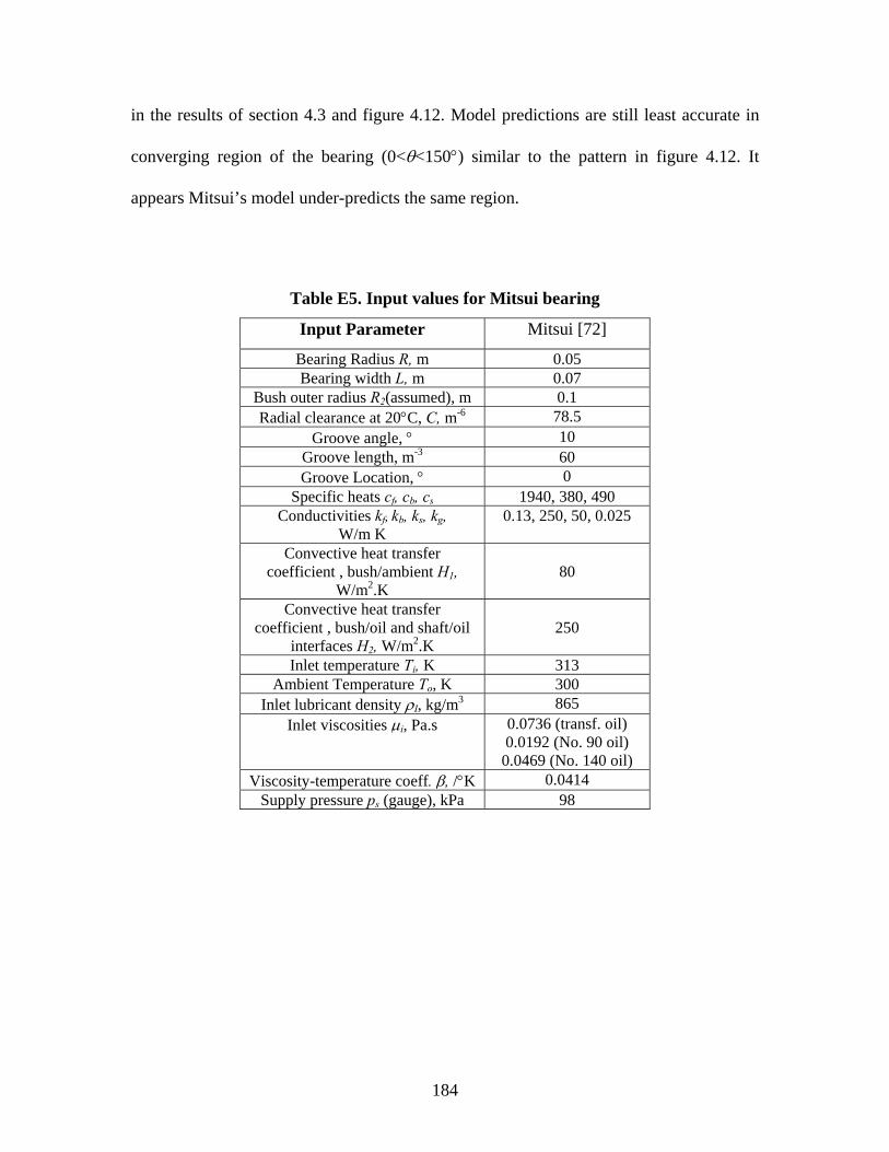
184
in the results of section 4.3 and figure 4.12. Model predictions are still least accurate in
converging region of the bearing (0<θ<150°) similar to the pattern in figure 4.12. It
appears Mitsui’s model under-predicts the same region.
Table E5. Input values for Mitsui bearing
Input Parameter Mitsui [72]
Bearing Radius R, m 0.05 Bearing width L, m 0.07
Bush outer radius R2(assumed), m 0.1 Radial clearance at 20°C, C, m-6 78.5
Groove angle, ° 10 Groove length, m-3 60 Groove Location, ° 0
Specific heats cf, cb, cs 1940, 380, 490 Conductivities kf, kb, ks, kg,
W/m K 0.13, 250, 50, 0.025
Convective heat transfer coefficient , bush/ambient H1,
W/m2.K
80
Convective heat transfer coefficient , bush/oil and shaft/oil
interfaces H2, W/m2.K
250
Inlet temperature Ti, K 313 Ambient Temperature To, K 300
Inlet lubricant density ρI, kg/m3 865 Inlet viscosities μi, Pa.s 0.0736 (transf. oil)
0.0192 (No. 90 oil) 0.0469 (No. 140 oil)
Viscosity-temperature coeff. β, /°K 0.0414 Supply pressure ps (gauge), kPa 98

185
Figure E6. SUPG predictions versus experimental temperatures, Mitusi [72]. Included is Mitsui’s prediction for no.90 oil.
A summary of the maximum and average errors for SUPG and Mitsui’s model are shown
in table E6. SUPG predictions are significantly better in each case.
Table E6 Maximum and average error for Mitsui’s data.
Error Summary Transformer oil No. 90 oil No. 140 oil SUPG Mitsui SUPG Mitsui SUPG Mitsui
Max Error 0.017 0.039 0.014 0.030 0.015 0.028 Ave. error 0.008 0.017 0.026 0.064 0.025 0.073
40
42
44
46
48
50
52
54
56
58
60
0 30 60 90 120 150 180 210 240 270 300 330 360
Tem
pera
ture
, C
Angle, degrees
Predictions vs Exp. Temperatures
Mitsui:No.140
No.140
No.90
Transformer
SUPG:Transf
SUPG:No.90
SUPG: No.140
Mitsui:No.90

186
E5. SUPG performance in predicting Pierre’s data
The data and THD model presented by Pierre and Fillon [73] is analyzed and compared
to SUPG predictions. The researchers present thermal and performance parameters for
bearing input data presented in table E7.
Table E7 Input parameters for journal tested [73]
Input Parameter [unit] Value
Diameter D, [m] 0.1 Bearing length L, [m] 0.08 Radial clearance C, [µm] 123 Rotational speed Ns, [rev/min] 3000 Oil supply temperature Ti, [°C] 35 and 50 Bearing load Wd, [N] 9000 Dynamic viscosity µì40°C at 40 °C (10-3 Pa.s) 30 Dynamic viscosity µì100°C at 100 °C (10-3 Pa.s) 4.05 Lubricant density ρ, [kg/m3] 860 Lubricant specific heat Cp, [J/kg.K] 2000
Experimental and predicted temperatures for the two speeds are shown in figure E7
(figure 2 in reference 73). Their THD model appears to be less accurate in the convergent
and divergent zones.

187
Figure E7. Experimental and THD temperature predictions as a function of angle from
inlet groove [73].
The two cases in figure E7 are analyzed using SUPG and presented in figure E8. Included
on figure E8(a) is Pierre’s prediction for reference. Table E7 gives a summary of the error
magnitudes from the two methods. These show SUPG to give better results in both cases.
Both models are off on the convergent region while SUPG gives more accurate
predictions in the divergent zone (240<θ<360).
Table E8 gives a summary of performance parameter predictions for Pierre’s data. L/D
ratio is 1, input oil temperature Ti is 40°C (other input parameters as shown in table E6).
The bearing characteristic number S. The error, as determined as before (equation E3) is
small, showing the accuracy of SUPG.
35
40
45
50
55
60
65
70
0 60 120 180 240 300 360
Tempe
rature, C
Angle from inlet groove, deg
Pierre's Model
T35Exp.T50Exp.Pierre@35CPierre@50C

188
(a)
(b)
Figure E8. Comparison of SUPG and Pierre’s THD model [73].
35
40
45
50
55
60
65
0 30 60 90 120 150 180 210 240 270 300 330 360
Tem
pera
ture
, C
Angle from groove pos., degrees
SUPG vs Pierre Predictions, Ti=35 C
Exp. DataSUPGPierre
40
45
50
55
60
65
70
0 30 60 90 120 150 180 210 240 270 300 330 360
Tem
pera
ture
, C
Angle from inlet groove, degrees
SUPG vs Pierre Predictions, Ti=50 C
Exp. dataSUPGPierre

189
Table E8. Error on thermal predictions, SUPG vs Pierre’s THD model
Error Summary T35 T50 SUPG Pierre SUPG Pierre Max Error 0.047 0.052 0.058 0.076Ave. error 0.105 0.128 0.029 0.037
Table E9. Performance parameter predictions for Pierre’s data
S=0.227 Exp. Data SUPG Error
PL 820 819.5 0.0006
pmax, MPa 2.3 2.26 0.0174
Tmax, C 58 59.5 0.0250QL, m3/s 4.50E-05 4.60E-05 0.0222


![1728EX+ : Programming Guide - safe-tech · 02 ... Streamline section Streamline Streamline section Streamline section ... 1728EX+ : Programming Guide Keywords [English] Created Date:](https://static.fdocuments.net/doc/165x107/5b84d6a77f8b9aec488d14a4/1728ex-programming-guide-safe-02-streamline-section-streamline-streamline.jpg)