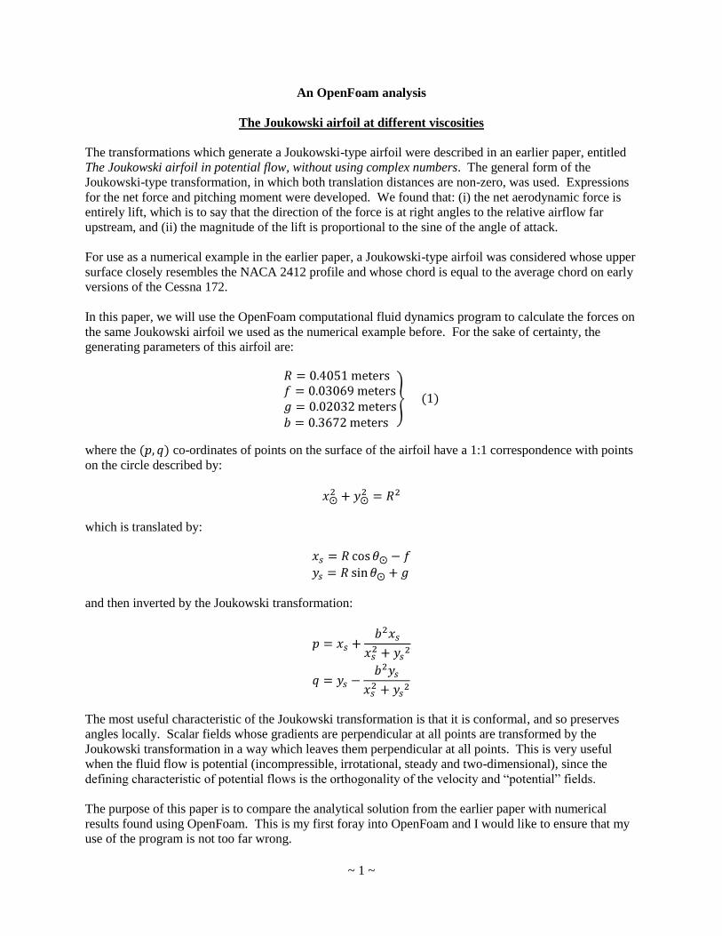
~ 1 ~

An OpenFoam analysis

The Joukowski airfoil at different viscosities

The transformations which generate a Joukowski-type airfoil were described in an earlier paper, entitled

The Joukowski airfoil in potential flow, without using complex numbers. The general form of the

Joukowski-type transformation, in which both translation distances are non-zero, was used. Expressions

for the net force and pitching moment were developed. We found that: (i) the net aerodynamic force is

entirely lift, which is to say that the direction of the force is at right angles to the relative airflow far

upstream, and (ii) the magnitude of the lift is proportional to the sine of the angle of attack.

For use as a numerical example in the earlier paper, a Joukowski-type airfoil was considered whose upper

surface closely resembles the NACA 2412 profile and whose chord is equal to the average chord on early

versions of the Cessna 172.

In this paper, we will use the OpenFoam computational fluid dynamics program to calculate the forces on

the same Joukowski airfoil we used as the numerical example before. For the sake of certainty, the

generating parameters of this airfoil are:

where the co-ordinates of points on the surface of the airfoil have a 1:1 correspondence with points

on the circle described by:

which is translated by:

and then inverted by the Joukowski transformation:

The most useful characteristic of the Joukowski transformation is that it is conformal, and so preserves

angles locally. Scalar fields whose gradients are perpendicular at all points are transformed by the

Joukowski transformation in a way which leaves them perpendicular at all points. This is very useful

when the fluid flow is potential (incompressible, irrotational, steady and two-dimensional), since the

defining characteristic of potential flows is the orthogonality of the velocity and “potential” fields.

The purpose of this paper is to compare the analytical solution from the earlier paper with numerical

results found using OpenFoam. This is my first foray into OpenFoam and I would like to ensure that my

use of the program is not too far wrong.

~ 2 ~

Meshing using GMesh

Computational fluid dynamics applies the equations for the fluid flow to discrete points in space (and in

time as well if one is looking at a non-steady state, or transient, flow). The surface of the airfoil needs to

be divided into short segments, the airfoil itself needs to be placed inside some bounded region of space,

which I will call a virtual wind tunnel, and the space to be occupied by the fluid needs to be discretized

into a mesh of small elements. I used the program GMesh to do these things. For a two-dimensional case

like this one, GMesh produces a mesh of small triangular prisms which extend from the front face of the

virtual wind tunnel through to the back face.

GMesh can take its instructions from a text file which contains the necessary commands in the prescribed

syntax. GMesh will write a second text file with lists of the vertices, faces and tetrahedra (or prisms) in a

format which OpenFoam can understand.

To assist in preparing the input text file, I wrote a program in Visual Basic 2010 Express which is listed in

Appendix “A”. The program starts with the parameters of the Joukowski airfoil in Equation above. It

generates the co-ordinates of the upper and lower surfaces. To be precise, it generates one million pairs

of co-ordinates on the two surfaces, from among which it selects the pairs which lie closest to the spacing

requirement specified by the user. The user can specify whether the points should be equally spaced or

weighted towards the leading and trailing edges. [The one million points are generated at angles equally

spaced around the source circle of the Joukowski airfoil. The corresponding points after the

transformations will not be equally spaced along the surface of the airfoil.] The user can also specify the

number of segments into which to divide the upper and lower surfaces. The default is 1000 segments, or

panels, per surface and the runs whose results are shown below are based on this number of segments.

Appendix “B” is a listing of certain parts of the file produced by GMesh in the case where the airfoil is

rotated to an angle of attack of 5°. Similar files were produced for angles of attack ranging from -5° to

25° at two-degree intervals. A mesh is produced for a given geometry, not for a given flight condition.

By this, I mean that the same mesh is used when the angle of attack is 5°, whether the air speed is 100

mph or 120 mph, or whether the altitude is sea level or 10,000 feet. The wind condition is set by the

parameters given to OpenFoam; the geometry is set by the parameters given to GMesh.

The virtual wind tunnel

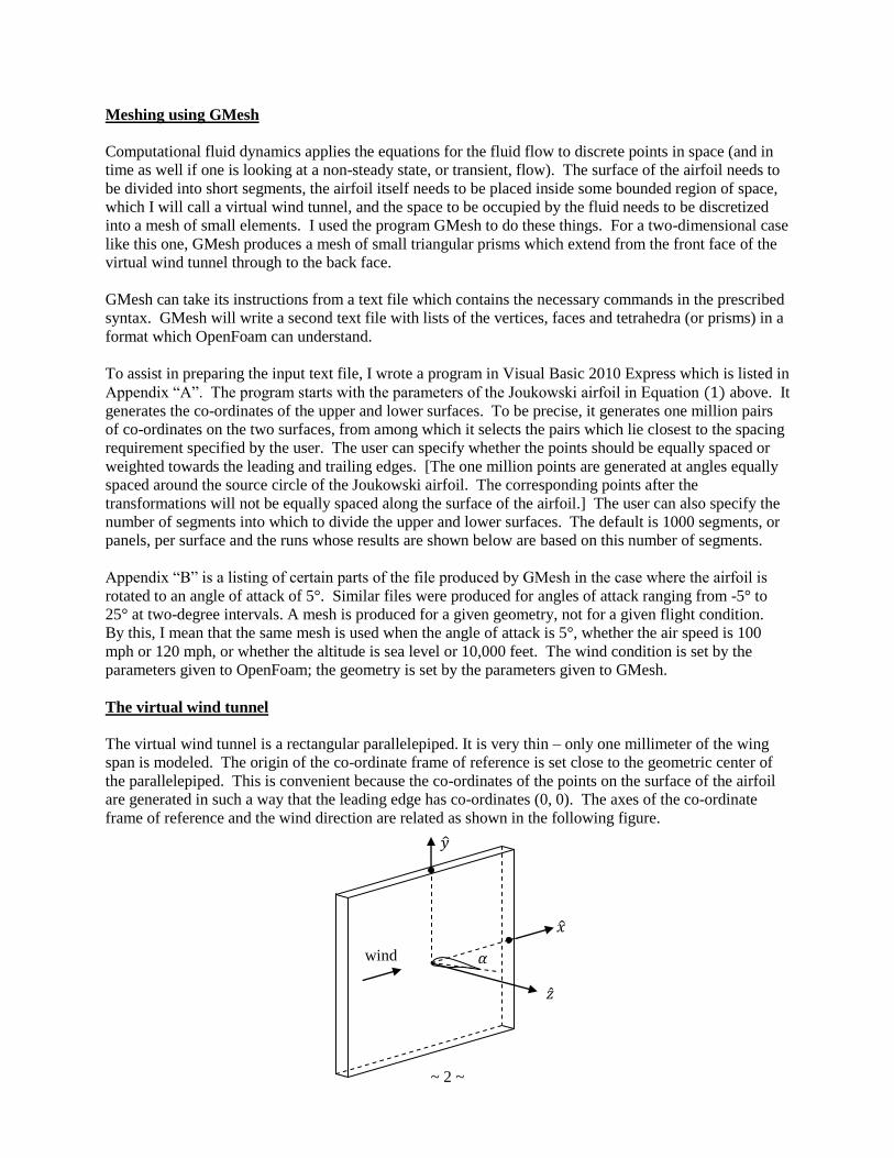
The virtual wind tunnel is a rectangular parallelepiped. It is very thin – only one millimeter of the wing

span is modeled. The origin of the co-ordinate frame of reference is set close to the geometric center of

the parallelepiped. This is convenient because the co-ordinates of the points on the surface of the airfoil

are generated in such a way that the leading edge has co-ordinates (0, 0). The axes of the co-ordinate

frame of reference and the wind direction are related as shown in the following figure.

wind

~ 3 ~

The relative wind is assumed to flow in the direction of the positive -axis. The -direction is “up” and

the -axis completes a standard right-handed co-ordinate frame of reference. The thickness of the wind

tunnel in the -direction has been exaggerated a little in the figure for clarity’s sake. The origin is located

halfway through the thickness, so the front and back faces of the wind tunnel are located at

, respectively. Since this is a two-dimensional analysis, it will not be necessary to solve

the equations for the fluid flow in the -direction, so the front and back faces are defined as “empty”

patches in OpenFoam’s /constant/polyMesh/boundary file.

It is convenient to specify the length and height of the wind tunnel in terms of the length of the airfoil’s

chord. All of the cases described below were run with the following wind tunnel dimensions:

distance from the leading edge / origin to the top face is 5 chord lengths,

distance from the leading edge / origin to the bottom face is 5.5 chord lengths,

distance from the leading edge / origin to the upwind face (“Inlet”) is 5 chord lengths and

distance from the leading edge / origin to the downwind face (“Outlet”) is 6 chord lengths.

The /constant/polyMesh/boundary file for the 5° angle of attack case (which I will sometimes call

the base case) is listed in Appendix “C”. As stated already, the front and back faces of the wind tunnel

are defined as “empty” patches. The top and bottom faces of the wind tunnel are defined as

“symmetryPlanes”, so that the pressure and velocity should be the same all along the face once the

solution converges. This is a less demanding requirement than setting specific values on these faces,

which gives the numerical routine more flexibility during each iteration while still converging to the same

end. The pressure was set to zero across the Inlet and Outlet. Since the forces on the airfoil arise from

differences in pressure at various points on the surface, the addition or subtraction of some constant value

to the static pressure does not affect them. For convenience, the upwind and downwind static pressures

were set to zero. The wind velocity was specified across the Inlet and Outlet as 44.704 meters per second,

equal to 100 miles per hour, in the -direction.

The characteristic lengths

GMesh permits the user to specify a “characteristic length” for every vertex, or point, that is defined

inside or on the virtual wind tunnel. When GMesh discretizes the fluid volume into small elements, it

tries to arrange things so that the mesh elements have edge-lengths equal to the characteristic length in

and around the vertex, or point, at which they are defined. GMesh then interpolates the sizes of the

elements elsewhere in the mesh to marry with the sizes at the vertices.

In all the runs done for this paper, the characteristic lengths were set as follows:

the characteristic length on the surface of the airfoil is 0.2 millimeters and

the characteristic length on the surface of the wind tunnel is 0.25 meters.

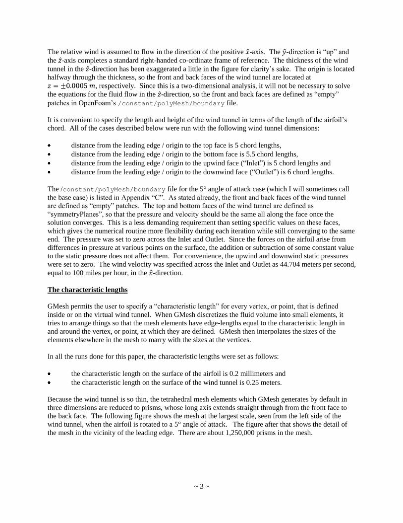
Because the wind tunnel is so thin, the tetrahedral mesh elements which GMesh generates by default in

three dimensions are reduced to prisms, whose long axis extends straight through from the front face to

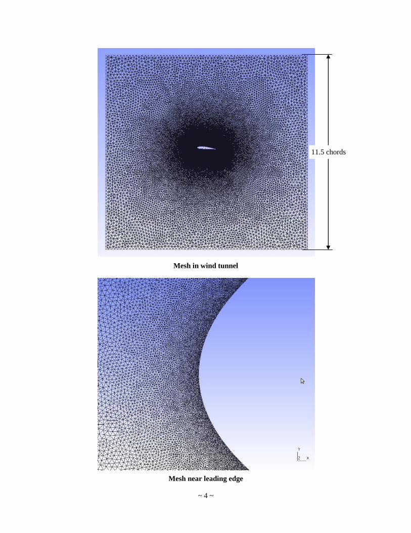
the back face. The following figure shows the mesh at the largest scale, seen from the left side of the

wind tunnel, when the airfoil is rotated to a 5° angle of attack. The figure after that shows the detail of

the mesh in the vicinity of the leading edge. There are about 1,250,000 prisms in the mesh.

~ 4 ~

Mesh in wind tunnel

Mesh near leading edge

11.5 chords

~ 5 ~

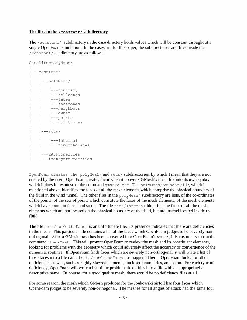
The files in the /constant/ subdirectory

The /constant/ subdirectory in the case directory holds values which will be constant throughout a

single OpenFoam simulation. In the cases run for this paper, the subdirectories and files inside the

/constant/ subdirectory are as follows.

CaseDirectoryName/

|

|---constant/

| |

| |---polyMesh/

| | |

| | |---boundary

| | |---cellZones

| | |---faces

| | |---faceZones

| | |---neighbour

| | |---owner

| | |---points

| | |---pointZones

| |

| |---sets/

| | |

| | |---Internal

| | |---nonOrthoFaces

| |

| |---RASProperties

| |---transportProerties

OpenFoam creates the polyMesh/ and sets/ subdirectories, by which I mean that they are not

created by the user. OpenFoam creates them when it converts GMesh’s mesh file into its own syntax,

which it does in response to the command gmshToFoam. The polyMesh/boundary file, which I

mentioned above, identifies the faces of all the mesh elements which comprise the physical boundary of

the fluid in the wind tunnel. The other files in the polyMesh/ subdirectory are lists, of the co-ordinates

of the points, of the sets of points which constitute the faces of the mesh elements, of the mesh elements

which have common faces, and so on. The file sets/Internal identifies the faces of all the mesh

elements which are not located on the physical boundary of the fluid, but are instead located inside the

fluid.

The file sets/nonOrthoFaces is an unfortunate file. Its presence indicates that there are deficiencies

in the mesh. This particular file contains a list of the faces which OpenFoam judges to be severely non-

orthogonal. After a GMesh mesh has been converted into OpenFoam’s syntax, it is customary to run the

command checkMesh. This will prompt OpenFoam to review the mesh and its constituent elements,

looking for problems with the geometry which could adversely affect the accuracy or convergence of the

numerical routines. If OpenFoam finds faces which are severely non-orthogonal, it will write a list of

those faces into a file named sets/nonOrthoFaces, as happened here. OpenFoam looks for other

deficiencies as well, such as highly-skewed elements, unclosed boundaries, and so on. For each type of

deficiency, OpenFoam will write a list of the problematic entities into a file with an appropriately

descriptive name. Of course, for a good quality mesh, there would be no deficiency files at all.

For some reason, the mesh which GMesh produces for the Joukowski airfoil has four faces which

OpenFoam judges to be severely non-orthogonal. The meshes for all angles of attack had the same four

~ 6 ~

such faces. I was not able to correct this problem. When GMesh generates a mesh for a two-dimensional

geometry, it does not allow any optimization. Fortunately, despite the existence of these four faces,

GMesh reported “Mesh OK”, and I proceeded with the imperfect mesh.

The files constant/RASProperties and constant/transportProperties are created by the user.

The former specifies the mathematical model of the turbulence to be used and the latter specifies the

transport properties of the fluid. In this study, I have chosen to use the Spalart-Allmaras turbulence

model, which is said to be pretty good for two-dimensional flows. I have assumed that the fluid is

Newtonian and, as a starting point, I have used the viscosity and density of air at sea level.

Appendix “D” is a listing of these two files for the base case.

The files in the /system/ subdirectory

The /system/ subdirectory in the case directory holds the settings which control the execution of an

OpenFoam run. In the cases run for this paper, the subdirectories and files inside the /system/

subdirectory are the following.

CaseDirectoryName/

|

|---system/

| |

| |---controlDict

| |---decomposeParDict

| |---fvSchemes

| |---fvSolution

The file decomposeParDict controls the decomposition of the geometry into separate pieces, in

preparation for execution by eight processors running in parallel. The file fvSchemes specifies the

mathematical routines to be used to approximate the equations in their discretized form. The file

fvSolution specifies how the physical variables should be derived from the equations of motion and

how they should be permitted to change during the process of converging to a solution.

Appendix “E” is a listing of these four files for the base case.

It should be noted that the file controlDict includes the declaration of a function which prints out the

pressure and viscous forces and moments after each iteration.

The files in the /0/ subdirectory

The /0/ subdirectory in the case directory holds the initial conditions for an OpenFoam simulation.

Although the simpleFoam solver seeks a steady-state solution, for which there are no initial conditions

per se, the “initial conditions” are treated as the starting estimates of the physical variables for use in the

first iteration. The physical variables include the usual suspects – the pressure p, the velocity field U and

the viscosity nu (or nut) – and also one more variable, nuTilda, which is a parameter used in the Spalart-

Allmaras turbulence model.

In the cases run for this paper, the files inside the /0/ subdirectory are as follows.

~ 7 ~

CaseDirectoryName/

|

|---0/

| |

| |---p

| |---U

| |---nut

| |---nuTilda

I have attacked as Appendix “F” a listing of these four files for the base case.

The pressure file (0/p) and velocity file (0/U) are pretty straight-forward. The pressure is set to zero on

the Inlet and Outlet faces of the wind tunnel. The wind velocity is set to 100 miles per hour on those

faces, as well. The actual surface of the airfoil, which is a physical “wall” as far as OpenFoam is

concerned, is treated as a no-slip wall on which the velocity is zero.

The nut and nuTilda files are a little different and contain the user’s (that is, my) estimates for these two

variables. There are a couple of rules of thumb which can be used to come up with these estimates. I

took guidance from certain webpages of “CFD-Wiki, the free CFD reference” at www.cfd-online.com.

A parameter called the “turbulence intensity” is defined for the Inlet of the virtual wind tunnel. It is

intended to measure the turbulence in the flow of the fluid as it approaches the body of interest. The

webpage gives some helpful examples. I quote:

1. “High-turbulence case: High-speed flow inside complex geometries like heat-exchangers and

flow inside rotating machinery (turbines and compressors). Typically the turbulence intensity is

between 5% and 20%.

2. “Medium-turbulence case: Flow in not-so-complex devices like large pipes, ventilation flows,

etc., or low speed flows (low Reynolds number). Typically the turbulence intensity is between

1% and 5%.

3. “Low-turbulence case: Flow originating from a fluid that stands still, like external flow across

cars, submarines and aircrafts. Very high-quality wind-tunnels can also reach really low

turbulence levels. Typically the turbulence intensity is very low, well below 1%.”

A parameter called the “turbulence length scale” is defined as the estimate of the size of the largest-scale

eddies in the turbulent flow. As a guide, the webpage says,

“It is common to set the turbulence length scale to a certain percentage of a typical dimension of

the problem. For example, at the inlet to a turbine stage a typical turbulence length scale could be

say 5% of the channel height. In grid-generated turbulence the turbulence length scale is often set

to something close to the size of the grid bars.”

In this study, the airfoil will be simulated at a range of angles of attack, including high angles of attack at

which there will be massive separation of the airfoil from the surface. The eddies which arise in these

cases will likely be an appreciable fraction of the length of the chord, perhaps 10% or more.

In a page entitled Turbulence free-stream boundary conditions, the turbulence intensity and turbulence

length scale are combined into the following estimate for nuTilda ( ):

~ 8 ~

This webpage makes a remark about the Spalart-Allmaras turbulence model, which is therefore relevant

for this study, that:

“Ideally with the Spalart-Allmaras model , but some solvers can have problem with that so

can be used. This is if the trip term is used to "start up" the model. A convenient option

is to set in the freestream. The model then provides fully turbulent results and any

regions like boundary layers that contain shear become fully turbulent.”

In the base case, and all the other runs made using the viscosity at sea level, I used the following

estimates:

Then, in the 0/nuTilda file, I defined the freestream as five times this value. In the 0/nut file, I

defined the viscosity as one-tenth of this value.

These are initial settings for the simulation. As the simulation proceeds, OpenFoam uses in own interim

calculations to improve the estimates. It is helpful if the initial estimates are as accurate as possible, but it

is not fatal to the procedure if they are wrong.

The results from the OpenFoam simulation of the base case

The base case assumes the kinematic viscosity of air at sea level ( ), the density of

air at sea level ( ) and a relative wind of 100 miles per hour ( ). In this section, I

will describe the results from the OpenFoam simulation and compare them with the results found

analytically in the earlier paper, in which potential flow was assumed.

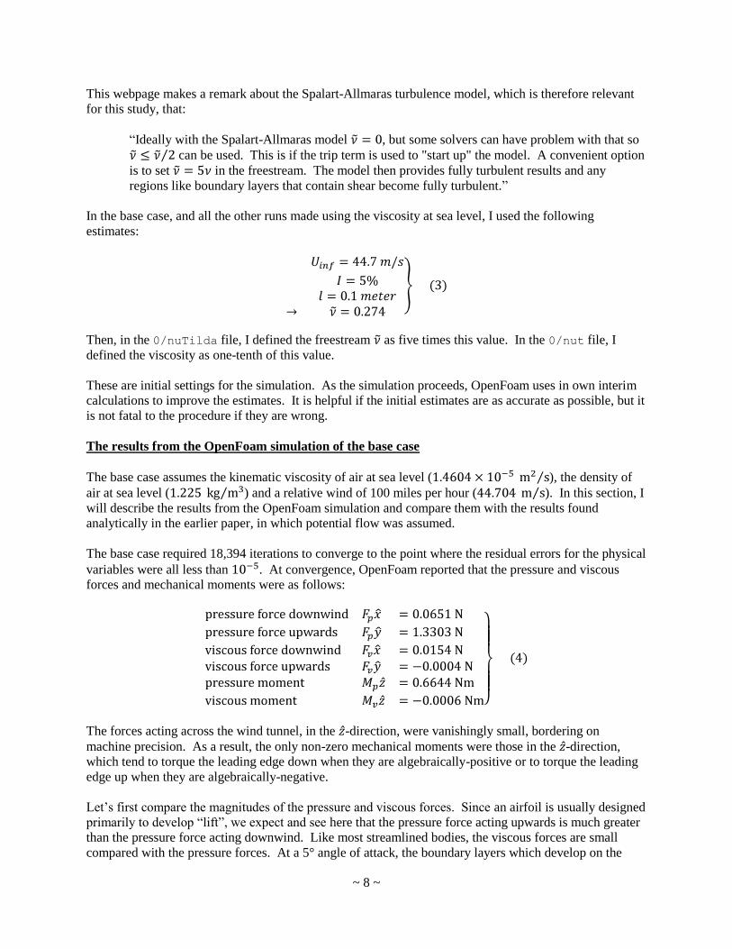
The base case required 18,394 iterations to converge to the point where the residual errors for the physical

variables were all less than . At convergence, OpenFoam reported that the pressure and viscous

forces and mechanical moments were as follows:

The forces acting across the wind tunnel, in the -direction, were vanishingly small, bordering on

machine precision. As a result, the only non-zero mechanical moments were those in the -direction,

which tend to torque the leading edge down when they are algebraically-positive or to torque the leading

edge up when they are algebraically-negative.

Let’s first compare the magnitudes of the pressure and viscous forces. Since an airfoil is usually designed

primarily to develop “lift”, we expect and see here that the pressure force acting upwards is much greater

than the pressure force acting downwind. Like most streamlined bodies, the viscous forces are small

compared with the pressure forces. At a 5° angle of attack, the boundary layers which develop on the

~ 9 ~

wind

upper and lower surfaces resist the flow of air much more in the direction parallel to the surface than in

the direction perpendicular to it. As a result, the magnitude of the viscous force acting downstream is

much larger than the magnitude of the viscous force acting upwards or downwards. And, in fact, what

little viscous force there is in the direction perpendicular to the relative wind, is directed downwards.

This makes sense intuitively – the airfoil is rotated downwards at its aft end, so the air which drags itself

along the surface is actually pulling downwards, hence the algebraically-negative viscous force .

Since the pressure forces are greater than the viscous forces, the mechanical moment they cause is greater

than the mechanical moment the viscous forces cause. The algebraically-positive net moment is in the

direction which forces the nose of the airfoil down.

Let’s now set aside the viscous forces and look only at the pressure forces. We can combine the two

components of the pressure force into its total magnitude and its direction, which we will measure as its

angle with respect to the -axis. The following figure shows the geometry.

In the figure, the airfoil is shown as simply a dot. The components of the pressure force are combined

using the Pythagorean Theorem, thus:

and the angle can be found using the inverse tangent function:

The total pressure force in Equation is the total pressure force acting on the section of the airfoil

inside the virtual wind tunnel. Recall that the wind tunnel is only one millimeter thick. A section of

airfoil one unit length, or one meter, in span, would experience 1000 times as much force, or .

The angle in Equation is about 2.8° past the vertical to the relative wind, where “past” means biased

downwind.

We can compare these figures to the ones we found analytically. When this airfoil was analyzed in a

potential flow, the pressure force was found to be exactly perpendicular to the relative wind. The total

~ 10 ~

pressure force was found to be . Of course, potential flow assumes, among other things, that

the viscosity is zero. The OpenFoam simulation was run assuming the airfoil was cruising in real air at

sea level. Perhaps one should be pleasantly surprised that the simplified assumptions of potential flow

give a total pressure force within 29% of that generated using OpenFoam.

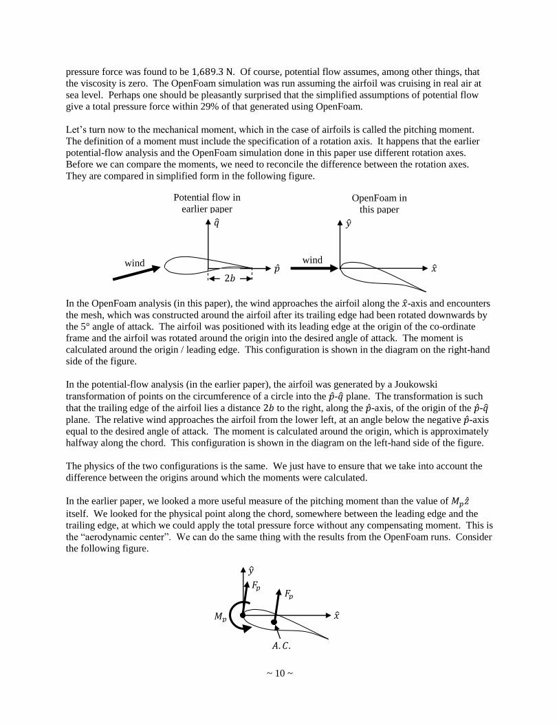
Let’s turn now to the mechanical moment, which in the case of airfoils is called the pitching moment.

The definition of a moment must include the specification of a rotation axis. It happens that the earlier

potential-flow analysis and the OpenFoam simulation done in this paper use different rotation axes.

Before we can compare the moments, we need to reconcile the difference between the rotation axes.

They are compared in simplified form in the following figure.

In the OpenFoam analysis (in this paper), the wind approaches the airfoil along the -axis and encounters

the mesh, which was constructed around the airfoil after its trailing edge had been rotated downwards by

the 5° angle of attack. The airfoil was positioned with its leading edge at the origin of the co-ordinate

frame and the airfoil was rotated around the origin into the desired angle of attack. The moment is

calculated around the origin / leading edge. This configuration is shown in the diagram on the right-hand

side of the figure.

In the potential-flow analysis (in the earlier paper), the airfoil was generated by a Joukowski

transformation of points on the circumference of a circle into the - plane. The transformation is such

that the trailing edge of the airfoil lies a distance to the right, along the -axis, of the origin of the -

plane. The relative wind approaches the airfoil from the lower left, at an angle below the negative -axis

equal to the desired angle of attack. The moment is calculated around the origin, which is approximately

halfway along the chord. This configuration is shown in the diagram on the left-hand side of the figure.

The physics of the two configurations is the same. We just have to ensure that we take into account the

difference between the origins around which the moments were calculated.

In the earlier paper, we looked a more useful measure of the pitching moment than the value of

itself. We looked for the physical point along the chord, somewhere between the leading edge and the

trailing edge, at which we could apply the total pressure force without any compensating moment. This is

the “aerodynamic center”. We can do the same thing with the results from the OpenFoam runs. Consider

the following figure.

wind

wind

Potential flow in

earlier paper OpenFoam in

this paper

~ 11 ~

When the total pressure force is applied at the leading edge, which is the origin in the OpenFoam frame of

reference, the moment is equal to , for the one millimeter section in the wind tunnel, or

per meter of span. We will translate the point of application of the force towards the trailing

edge until we find the point at which the accompanying moment is zero.

Moving some distance along the chord is equivalent to moving a distance along the -

axis and a distance along the -axis, where is the angle of attack. Distance will be

the moment arm through which the vertical component of the pressure force exerts a nose-down

moment around the leading edge. Similarly, distance (the positive distance) will be the moment arm

through which the horizontal component of the pressure force also exerts a nose-down moment

around the leading edge. When translation by distance gives a combined nose-down moment equal to

zero, we will have arrived at the aerodynamic center. This will happen mathematically when:

The numerical values in the base case are:

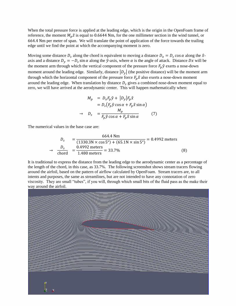
It is traditional to express the distance from the leading edge to the aerodynamic center as a percentage of

the length of the chord, in this case, as 33.7%. The following screenshot shows stream tracers flowing

around the airfoil, based on the pattern of airflow calculated by OpenFoam. Stream tracers are, to all

intents and purposes, the same as streamlines, but are not intended to have any connotation of zero

viscosity. They are small “tubes”, if you will, through which small bits of the fluid pass as the make their

way around the airfoil.

~ 12 ~

The pattern of the airflow looks very similar to the pattern of the airflow we found when we examined

this airfoil in potential flow. The source line for the stream tracers in the figure is a vertical line located

two meters upwind from the leading edge. It extends from one meter below the leading edge to one-half

meter above. The source line is located a very small distance, 0.1 millimeters, to the left side (towards us,

on this side of the paper) of the central plane through the wind tunnel, simply to avoid any small

perturbations which may be associated with the mesh. There are 200 individual stream tracers, generated

at equally-spaced intervals along the source line.

.

The results from the OpenFoam simulation using sea level air conditions

In this section, we will look at the results when the airfoil is positioned at various angles of attack, not just

5°. In all of these cases, the relative wind speed is 100 miles per hour and the density and viscosity of the

air are their sea level values, per the U.S. Standard Atmosphere.

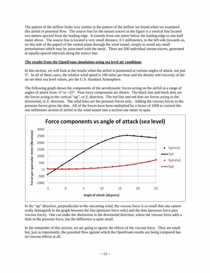
The following graph shows the components of the aerodynamic forces acting on the airfoil at a range of

angles of attack from -5° to +25°. Four force components are shown. The black line and black dots are

the forces acting in the vertical “up”, or , direction. The red line and red dots are forces acting in the

downwind, or , direction. The solid lines are the pressure forces only. Adding the viscous forces to the

pressure forces gives the dots. All of the forces have been multiplied by a factor of 1000 to convert the

one millimeter section of airfoil in the wind tunnel into a section one meter in span.

In the “up” direction, perpendicular to the oncoming wind, the viscous force is so small that one cannot

really distinguish in the graph between the line (pressure force only) and the dots (pressure force plus

viscous force). One can make the distinction in the downwind direction, where the viscous force adds a

little to the pressure force, but the difference is quite small.

In the remainder of this section, we are going to ignore the effects of the viscous force. They are small

but, just as importantly, the potential flow against which the OpenFoam results are being compared has

no viscous effects at all.

~ 13 ~

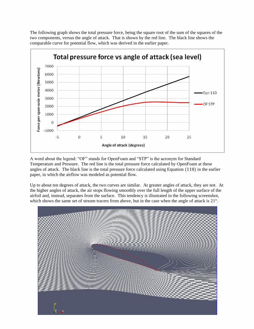
The following graph shows the total pressure force, being the square root of the sum of the squares of the

two components, versus the angle of attack. That is shown by the red line. The black line shows the

comparable curve for potential flow, which was derived in the earlier paper.

A word about the legend: “OF” stands for OpenFoam and “STP” is the acronym for Standard

Temperature and Pressure. The red line is the total pressure force calculated by OpenFoam at these

angles of attack. The black line is the total pressure force calculated using Equation in the earlier

paper, in which the airflow was modeled as potential flow.

Up to about ten degrees of attack, the two curves are similar. At greater angles of attack, they are not. At

the higher angles of attack, the air stops flowing smoothly over the full length of the upper surface of the

airfoil and, instead, separates from the surface. This tendency is illustrated in the following screenshot,

which shows the same set of stream tracers from above, but in the case when the angle of attack is 21°.

~ 14 ~

The airflow separates from the surface not far from the point of maximum thickness. It circles back

towards the trailing edge, defining something like a bubble on the upper surface. There is air inside the

bubble, and it will be moving violently around, in eddies of various scales. On the whole however, the air

in the bubble will not be moving as fast as the air in the stream tracer which just bounds the bubble. This

is important. With the right tweaking, or interpretation, Bernoulli’s Principle still applies: the reduction

in static pressure on the surface of the airfoil is proportional to the square of the air speed near the surface.

When a high speed streamline or stream tracer runs along the upper surface, the static pressure is reduced,

giving greater scope for the pressure acting on the lower surface of the airfoil to push upwards. If that

high speed streamline or stream tracer is replaced with the more confused flow inside a bubble, the static

pressure is higher than it otherwise would be, and the net lift on the airfoil is less than it otherwise would

be.

When the angle of attack is modest, say less than ten degrees, a small increase in the angle of attack leads

to a pattern of airflow where the speed of the air flowing over the top surface increases, leading to an

increase in the lift generated by the airfoil. Once the airfoil has stalled, and the flow separated from the

surface, further increases in the angle of attack just create more turbulence in the bubble, but not greater

lift.

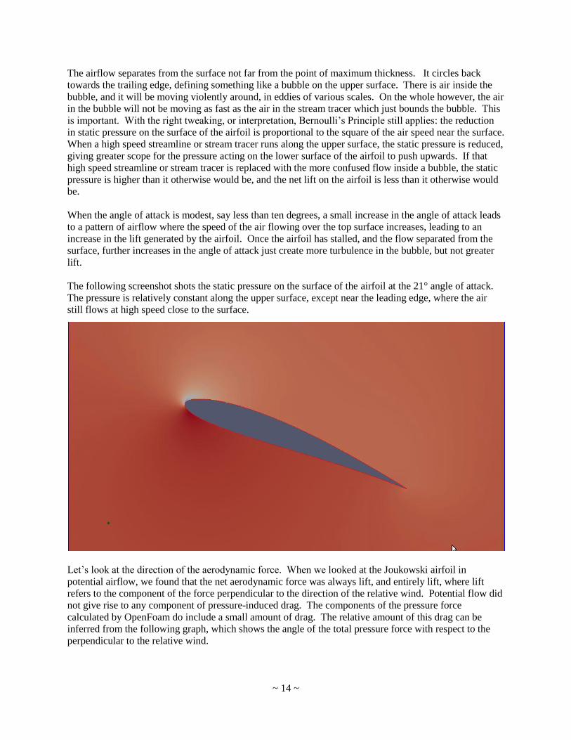
The following screenshot shots the static pressure on the surface of the airfoil at the 21° angle of attack.

The pressure is relatively constant along the upper surface, except near the leading edge, where the air

still flows at high speed close to the surface.

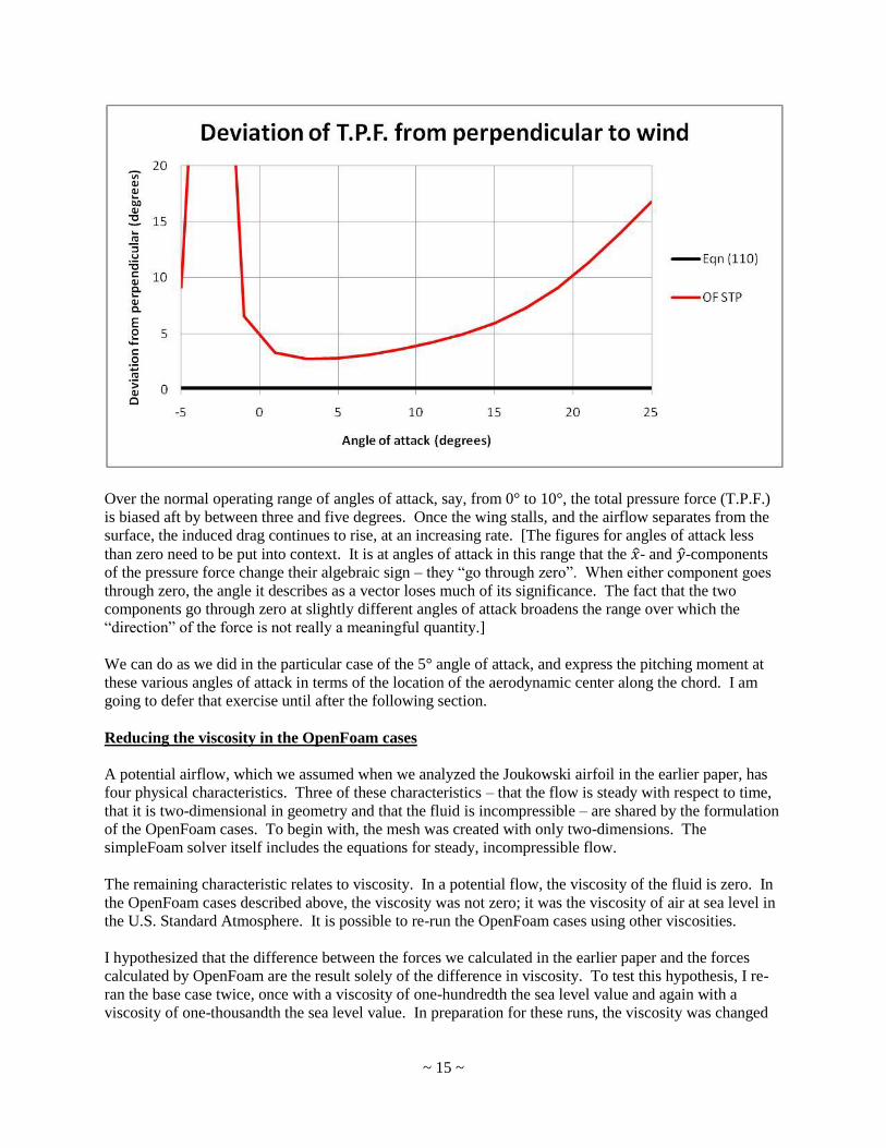
Let’s look at the direction of the aerodynamic force. When we looked at the Joukowski airfoil in

potential airflow, we found that the net aerodynamic force was always lift, and entirely lift, where lift

refers to the component of the force perpendicular to the direction of the relative wind. Potential flow did

not give rise to any component of pressure-induced drag. The components of the pressure force

calculated by OpenFoam do include a small amount of drag. The relative amount of this drag can be

inferred from the following graph, which shows the angle of the total pressure force with respect to the

perpendicular to the relative wind.

~ 15 ~

Over the normal operating range of angles of attack, say, from 0° to 10°, the total pressure force (T.P.F.)

is biased aft by between three and five degrees. Once the wing stalls, and the airflow separates from the

surface, the induced drag continues to rise, at an increasing rate. [The figures for angles of attack less

than zero need to be put into context. It is at angles of attack in this range that the - and -components

of the pressure force change their algebraic sign – they “go through zero”. When either component goes

through zero, the angle it describes as a vector loses much of its significance. The fact that the two

components go through zero at slightly different angles of attack broadens the range over which the

“direction” of the force is not really a meaningful quantity.]

We can do as we did in the particular case of the 5° angle of attack, and express the pitching moment at

these various angles of attack in terms of the location of the aerodynamic center along the chord. I am

going to defer that exercise until after the following section.

Reducing the viscosity in the OpenFoam cases

A potential airflow, which we assumed when we analyzed the Joukowski airfoil in the earlier paper, has

four physical characteristics. Three of these characteristics – that the flow is steady with respect to time,

that it is two-dimensional in geometry and that the fluid is incompressible – are shared by the formulation

of the OpenFoam cases. To begin with, the mesh was created with only two-dimensions. The

simpleFoam solver itself includes the equations for steady, incompressible flow.

The remaining characteristic relates to viscosity. In a potential flow, the viscosity of the fluid is zero. In

the OpenFoam cases described above, the viscosity was not zero; it was the viscosity of air at sea level in

the U.S. Standard Atmosphere. It is possible to re-run the OpenFoam cases using other viscosities.

I hypothesized that the difference between the forces we calculated in the earlier paper and the forces

calculated by OpenFoam are the result solely of the difference in viscosity. To test this hypothesis, I re-

ran the base case twice, once with a viscosity of one-hundredth the sea level value and again with a

viscosity of one-thousandth the sea level value. In preparation for these runs, the viscosity was changed

~ 16 ~

in three of the files in the case directory: in constant/transportProperties, in 0/nut and in

0/nuTilda.

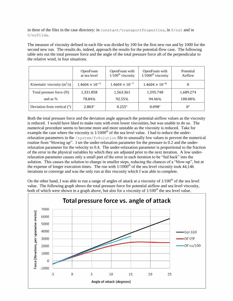
The measure of viscosity defined in each file was divided by 100 for the first new run and by 1000 for the

second new run. The results do, indeed, approach the results for the potential-flow case. The following

table sets out the total pressure force and the angle of the total pressure force aft of the perpendicular to

the relative wind, in four situations.

OpenFoam

at sea level

OpenFoam with

1/100th

viscosity

OpenFoam with

1/1000th viscosity

Potential

Airflow

Kinematic viscosity (m2/s)

Total pressure force (N)

and as %

Deviation from vertical (°)

Both the total pressure force and the deviation angle approach the potential-airflow values as the viscosity

is reduced. I would have liked to make runs with even lower viscosities, but was unable to do so. The

numerical procedure seems to become more and more unstable as the viscosity is reduced. Take for

example the case where the viscosity is 1/1000th of the sea level value. I had to reduce the under-

relaxation parameters in the /system/fvSolution file to unusually low values to prevent the numerical

routine from “blowing up”. I set the under-relaxation parameter for the pressure to 0.2 and the under-

relaxation parameter for the velocity to 0.4. The under-relaxation parameter is proportional to the fraction

of the error in the physical variables by which they are adjusted prior to the next iteration. A low under-

relaxation parameter causes only a small part of the error in each iteration to be “fed back” into the

solution. This causes the solution to change in smaller steps, reducing the chances of a “blow-up”, but at

the expense of longer execution times. The run with 1/1000th of the sea level viscosity took 44,146

iterations to converge and was the only run at this viscosity which I was able to complete.

On the other hand, I was able to run a range of angles of attack at a viscosity of 1/100th of the sea level

value. The following graph shows the total pressure force for potential airflow and sea level viscosity,

both of which were shown in a graph above, but also for a viscosity of 1/100th the sea level value.

~ 17 ~

As in the previous graph, the black line is the total pressure force for potential airflow and the red line is

the total pressure force from the first set of OpenFoam cases, run with sea level viscosity. The blue line is

the total pressure force with 1/100th of sea level viscosity. It is much closer to the potential airflow result,

and does not show any effects of stall / separation of flow, at least up to an angle of attack of 15°.

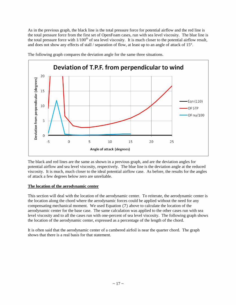
The following graph compares the deviation angle for the same three situations.

The black and red lines are the same as shown in a previous graph, and are the deviation angles for

potential airflow and sea level viscosity, respectively. The blue line is the deviation angle at the reduced

viscosity. It is much, much closer to the ideal potential airflow case. As before, the results for the angles

of attack a few degrees below zero are unreliable.

The location of the aerodynamic center

This section will deal with the location of the aerodynamic center. To reiterate, the aerodynamic center is

the location along the chord where the aerodynamic forces could be applied without the need for any

compensating mechanical moment. We used Equation above to calculate the location of the

aerodynamic center for the base case. The same calculation was applied to the other cases run with sea

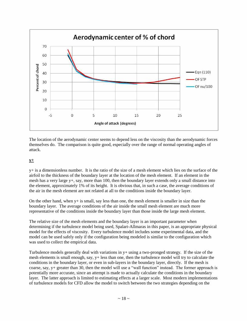
level viscosity and to all the cases run with one-percent of sea level viscosity. The following graph shows

the location of the aerodynamic center, expressed as a percentage of the length of the chord.

It is often said that the aerodynamic center of a cambered airfoil is near the quarter chord. The graph

shows that there is a real basis for that statement.

~ 18 ~

The location of the aerodynamic center seems to depend less on the viscosity than the aerodynamic forces

themselves do. The comparison is quite good, especially over the range of normal operating angles of

attack.

y+

y+ is a dimensionless number. It is the ratio of the size of a mesh element which lies on the surface of the

airfoil to the thickness of the boundary layer at the location of the mesh element. If an element in the

mesh has a very large y+, say, more than 100, then the boundary layer extends only a small distance into

the element, approximately 1% of its height. It is obvious that, in such a case, the average conditions of

the air in the mesh element are not related at all to the conditions inside the boundary layer.

On the other hand, when y+ is small, say less than one, the mesh element is smaller in size than the

boundary layer. The average conditions of the air inside the small mesh element are much more

representative of the conditions inside the boundary layer than those inside the large mesh element.

The relative size of the mesh elements and the boundary layer is an important parameter when

determining if the turbulence model being used, Spalart-Allmaras in this paper, is an appropriate physical

model for the effects of viscosity. Every turbulence model includes some experimental data, and the

model can be used safely only if the configuration being modeled is similar to the configuration which

was used to collect the empirical data.

Turbulence models generally deal with variations in y+ using a two-pronged strategy. If the size of the

mesh elements is small enough, say, y+ less than one, then the turbulence model will try to calculate the

conditions in the boundary layer, or even in sub-layers in the boundary layer, directly. If the mesh is

coarse, say, y+ greater than 30, then the model will use a “wall function” instead. The former approach is

potentially more accurate, since an attempt is made to actually calculate the conditions in the boundary

layer. The latter approach is limited to estimating effects at a larger scale. Most modern implementations

of turbulence models for CFD allow the model to switch between the two strategies depending on the

~ 19 ~

local value of y+. OpenFoam’s implementation of the Spalart-Allmaras turbulence model includes such

an automatic switch.

In the base case defined in this paper, where the airfoil is held at a 5° angle of attack to a 100 mile per

hour relative wind, the average y+ on the surface of the airfoil is 7.85. A separate value of y+ can be

calculated for each mesh element which has a face on the surface of the airfoil. The values of y+ for the

individual mesh elements ranged from a low y+ of 0.04 to a high y+ of 19.3. The Spalart-Allmaras model

should prove satisfactory when used in this range.

In the cases run with 1/100th of sea level viscosity, one expects that the reduced viscosity would cause the

boundary layer to be much thinner and, given that the same mesh is used, the calculated values of y+ to

be much higher. When the airfoil is held at a 5° angle of attack to a 100 mile per hour relative wind, and

the viscosity is 1/100th of its sea level value, the average y+ on the surface of the airfoil is 422, with a

minimum of 3.5 and a maximum of 1183. This configuration is at the limits of the applicability of the

Spalart-Allmaras turbulence model, which is said to decrease in accuracy once y+ exceeds 300. If time

permitted, it would be wise to re-run one or more of these low viscosity cases with a finer mesh. More

study is needed.

When the viscosity is reduced by another factor of ten, to 1/1000th of its sea level value, the calculated y+

increases even further. The average y+ is found to be 3550, with a minimum of 18.4 and a maximum of

10,007. While y+ at some of the mesh elements on the surface seems satisfactory, the average mesh

element is so much greater than 300 (the nominal maximum value of y+ which Spalart-Allmaras is

intended to accommodate), that we cannot rely on the results of this run.

This concludes my OpenFoam analysis of the Joukowski airfoil.

Jim Hawley

June 2013

An email setting out errors and omissions would be appreciated.

~ 20 ~

Appendix “A”

A Visual Basic program to produce an input file for GMesh

The program consists of the main windows form (Class Main) and three modules. Class Main manages

the GUI through which the user can change default values. Module Variables declares and sets values for

certain global variables. Module Joukowski calculates the co-ordinates of points on the surface of the

airfoil and module GMesh writes the necessary instructions to the output text file.

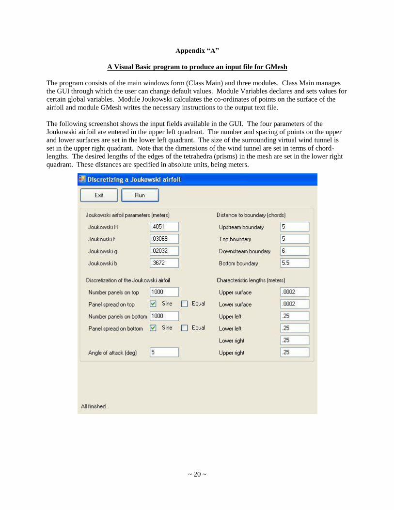
The following screenshot shows the input fields available in the GUI. The four parameters of the

Joukowski airfoil are entered in the upper left quadrant. The number and spacing of points on the upper

and lower surfaces are set in the lower left quadrant. The size of the surrounding virtual wind tunnel is

set in the upper right quadrant. Note that the dimensions of the wind tunnel are set in terms of chord-

lengths. The desired lengths of the edges of the tetrahedra (prisms) in the mesh are set in the lower right

quadrant. These distances are specified in absolute units, being meters.

~ 21 ~

Listing of class Main

Option Strict On Option Explicit On ' Discretizing a Joukowski airfoil Public Class Main Inherits System.Windows.Forms.Form Public Sub New() InitializeComponent() With Me Name = "" Text = "Discretizing a Joukowski airfoil" FormBorderStyle = Windows.Forms.FormBorderStyle.FixedSingle Size = New Drawing.Size(1024, 720) CenterToScreen() Visible = True Controls.Add(buttonExit) Controls.Add(buttonRun) Controls.Add(GroupboxEdit) Controls.Add(DisplayText) PerformLayout() End With End Sub '//////////////////////////////////////////////////////////////////////////////////// '//////////////////////////////////////////////////////////////////////////////////// '// Principal controls and handlers. '//////////////////////////////////////////////////////////////////////////////////// '//////////////////////////////////////////////////////////////////////////////////// Public WithEvents buttonExit As New Windows.Forms.Button With _ {.Size = New Drawing.Size(80, 30), _ .Location = New Drawing.Point(5, 5), _ .Text = "Exit", .TextAlign = ContentAlignment.MiddleCenter} Public Sub buttonExit_Click() Handles buttonExit.MouseClick Application.Exit() End Sub Public WithEvents buttonRun As New Windows.Forms.Button With _ {.Size = New Drawing.Size(80, 30), _ .Location = New Drawing.Point(90, 5), _ .Text = "Run", .TextAlign = ContentAlignment.MiddleCenter} Public Sub buttonRun_Click() Handles buttonRun.MouseClick MainProgram() End Sub Public GroupboxEdit As New Windows.Forms.GroupBox With _ {.Size = New Drawing.Size(485, 325), _ .Location = New Drawing.Point(5, 40)} Public DisplayText As New Windows.Forms.Label With _ {.Size = New Drawing.Size(300, 250), _ .Location = New Drawing.Point(5, 450), _ .Text = "", .TextAlign = ContentAlignment.TopLeft}

~ 22 ~

'//////////////////////////////////////////////////////////////////////////////////// '//////////////////////////////////////////////////////////////////////////////////// '// Main program. '//////////////////////////////////////////////////////////////////////////////////// '//////////////////////////////////////////////////////////////////////////////////// Public Sub MainProgram() ' ' Read the parameters from groupboxEdit. ReadParameters() ' ' Build the Joukowski airfoil. DisplayText.Text = "Now building Joukowski airfoil ..." & vbCrLf DisplayText.Refresh() JOUK_Airfoil() ' ' Align the Joukowski airfoil. DisplayText.Text = "Now aligning the airfoil ..." DisplayText.Refresh() JOUK_Align() ' ' Determine the surface points to send to GMesh. DisplayText.Text = "Now discretizing the airfoil for GMesh ..." DisplayText.Refresh() JOUK_Discretize() ' ' Rotate the airfoil to the angle of attack. DisplayText.Text = "Now rotating to the angle of attack ..." DisplayText.Refresh() JOUK_Rotate() ' ' Scale the distances expressed in chords into meters DistanceIm = -DistanceIc * JOUKchord DistanceTm = DistanceTc * JOUKchord DistanceRm = DistanceRc * JOUKchord DistanceOm = -DistanceOc * JOUKchord ' ' Now building the output file to send to GMesh. DisplayText.Text = "Now building the output file ..." DisplayText.Refresh() BuildGMeshFile() ' ' All finished. DisplayText.Text = "All finished." DisplayText.Refresh() End Sub '//////////////////////////////////////////////////////////////////////////////////// '//////////////////////////////////////////////////////////////////////////////////// '// Subroutine to read date from groupboxEdit. '//////////////////////////////////////////////////////////////////////////////////// '//////////////////////////////////////////////////////////////////////////////////// Public Sub ReadParameters() JOUKR = Val(tbR.Text) JOUKf = Val(tbF.Text) JOUKg = Val(tbG.Text) JOUKb = Val(tbB.Text) NumUpper = CInt(Val(tbNumU.Text)) NumLower = CInt(Val(tbNumL.Text)) AngleAttack = Val(tbAA.Text)

~ 23 ~

OutputFileName = "Joukowski_" & Trim(Str(AngleAttack)) & "deg.geo.txt" DistanceIc = Val(tbDisF.Text) DistanceTc = Val(tbDisT.Text) DistanceRc = Val(tbDisR.Text) DistanceOc = Val(tbDisB.Text) CharLenUm = Val(tbCharLenU.Text) CharLenLm = Val(tbCharLenL.Text) CharLenULm = Val(tbCharLenUL.Text) CharLenLLm = Val(tbCharLenLL.Text) CharLenLRm = Val(tbCharLenLR.Text) CharLenURm = Val(tbCharLenUR.Text) End Sub '//////////////////////////////////////////////////////////////////////////////////// '//////////////////////////////////////////////////////////////////////////////////// '// Controls to enter data. Note that there are four blocks, or Groups, of data. '//////////////////////////////////////////////////////////////////////////////////// '//////////////////////////////////////////////////////////////////////////////////// Public RowGroup1 As Int32 = 10 Public RowGroup2 As Int32 = RowGroup1 + 135 Public RowGroup3 As Int32 = RowGroup1 Public RowGroup4 As Int32 = RowGroup1 + 135 Public ColGroup1 As Int32 = 10 Public ColGroup2 As Int32 = ColGroup1 Public ColGroup3 As Int32 = ColGroup1 + 270 Public ColGroup4 As Int32 = ColGroup1 + 270 Public TitleW As Int32 = 180 Public LabelCol As Int32 = 5 Public LabelW As Int32 = 130 Public ValueCol As Int32 = 135 Public ValueW As Int32 = 60 Public labelGroup1 As New Windows.Forms.Label With _ {.Size = New Drawing.Size(TitleW, 20), _ .Location = New Drawing.Point(ColGroup1, RowGroup1), _ .Text = "Joukowski airfoil parameters (meters)", _ .TextAlign = ContentAlignment.MiddleLeft, _ .Parent = GroupboxEdit} Public labelR As New Windows.Forms.Label With _ {.Size = New Drawing.Size(LabelW, 20), _ .Location = New Drawing.Point(ColGroup1 + LabelCol, RowGroup1 + 25), _ .Text = "Joukowski R", .TextAlign = ContentAlignment.MiddleLeft, _ .Parent = GroupboxEdit} Public tbR As New Windows.Forms.TextBox With _ {.Size = New Drawing.Size(ValueW, 20), _ .Location = New Drawing.Point(ColGroup1 + ValueCol, RowGroup1 + 25), _ .Text = Trim(Str(JOUKR)), .TextAlign = HorizontalAlignment.Left, _ .Parent = GroupboxEdit} Public labelF As New Windows.Forms.Label With _ {.Size = New Drawing.Size(LabelW, 20), _ .Location = New Drawing.Point(ColGroup1 + LabelCol, RowGroup1 + 50), _ .Text = "Joukouski f", .TextAlign = ContentAlignment.MiddleLeft, _ .Parent = GroupboxEdit} Public tbF As New Windows.Forms.TextBox With _ {.Size = New Drawing.Size(ValueW, 20), _ .Location = New Drawing.Point(ColGroup1 + ValueCol, RowGroup1 + 50), _

~ 24 ~

.Text = Trim(Str(JOUKf)), .TextAlign = HorizontalAlignment.Left, _ .Parent = GroupboxEdit} Public labelG As New Windows.Forms.Label With _ {.Size = New Drawing.Size(LabelW, 20), _ .Location = New Drawing.Point(ColGroup1 + LabelCol, RowGroup1 + 75), _ .Text = "Joukowski g", .TextAlign = ContentAlignment.MiddleLeft, _ .Parent = GroupboxEdit} Public tbG As New Windows.Forms.TextBox With _ {.Size = New Drawing.Size(ValueW, 20), _ .Location = New Drawing.Point(ColGroup1 + ValueCol, RowGroup1 + 75), _ .Text = Trim(Str(JOUKg)), .TextAlign = HorizontalAlignment.Left, _ .Parent = GroupboxEdit} Public labelB As New Windows.Forms.Label With _ {.Size = New Drawing.Size(LabelW, 20), _ .Location = New Drawing.Point(ColGroup1 + LabelCol, RowGroup1 + 100), _ .Text = "Joukowski b", .TextAlign = ContentAlignment.MiddleLeft, _ .Parent = GroupboxEdit} Public tbB As New Windows.Forms.TextBox With _ {.Size = New Drawing.Size(ValueW, 20), _ .Location = New Drawing.Point(ColGroup1 + ValueCol, RowGroup1 + 100), _ .Text = Trim(Str(JOUKb)), .TextAlign = HorizontalAlignment.Left, _ .Parent = GroupboxEdit} Public labelGroup2 As New Windows.Forms.Label With _ {.Size = New Drawing.Size(TitleW, 20), _ .Location = New Drawing.Point(ColGroup2, RowGroup2), _ .Text = "Discretization of the Joukowski airfoil", _ .TextAlign = ContentAlignment.MiddleLeft, _ .Parent = GroupboxEdit} Public labelNumU As New Windows.Forms.Label With _ {.Size = New Drawing.Size(LabelW, 20), _ .Location = New Drawing.Point(ColGroup2 + LabelCol, RowGroup2 + 25), _ .Text = "Number panels on top", .TextAlign = ContentAlignment.MiddleLeft, _ .Parent = GroupboxEdit} Public tbNumU As New Windows.Forms.TextBox With _ {.Size = New Drawing.Size(ValueW, 20), _ .Location = New Drawing.Point(ColGroup2 + ValueCol, RowGroup2 + 25), _ .Text = Trim(Str(NumUpper)), .TextAlign = HorizontalAlignment.Left, _ .Parent = GroupboxEdit} Public labelSpreadU As New Windows.Forms.Label With _ {.Size = New Drawing.Size(LabelW, 20), _ .Location = New Drawing.Point(ColGroup2 + LabelCol, RowGroup2 + 50), _ .Text = "Panel spread on top", .TextAlign = ContentAlignment.MiddleLeft, _ .Parent = GroupboxEdit} Public WithEvents cbSpreadUSine As New Windows.Forms.CheckBox With _ {.Size = New Drawing.Size(ValueW, 20), _ .Location = New Drawing.Point(ColGroup2 + ValueCol, RowGroup2 + 50), _ .Text = "Sine", .TextAlign = ContentAlignment.MiddleCenter, _ .Checked = True, _ .Parent = GroupboxEdit} Public WithEvents cbSpreadUEqual As New Windows.Forms.CheckBox With _ {.Size = New Drawing.Size(ValueW, 20), _

~ 25 ~

.Location = New Drawing.Point(ColGroup2 + ValueCol + 65, RowGroup2 + 50), _ .Text = "Equal", .TextAlign = ContentAlignment.MiddleCenter, _ .Checked = False, _ .Parent = GroupboxEdit} Public labelNumL As New Windows.Forms.Label With _ {.Size = New Drawing.Size(LabelW, 20), _ .Location = New Drawing.Point(ColGroup2 + LabelCol, RowGroup2 + 75), _ .Text = "Number panels on bottom", .TextAlign = ContentAlignment.MiddleLeft, _ .Parent = GroupboxEdit} Public tbNumL As New Windows.Forms.TextBox With _ {.Size = New Drawing.Size(ValueW, 20), _ .Location = New Drawing.Point(ColGroup2 + ValueCol, RowGroup2 + 75), _ .Text = Trim(Str(NumLower)), .TextAlign = HorizontalAlignment.Left, _ .Parent = GroupboxEdit} Public labelSpreadL As New Windows.Forms.Label With _ {.Size = New Drawing.Size(LabelW, 20), _ .Location = New Drawing.Point(ColGroup2 + LabelCol, RowGroup2 + 100), _ .Text = "Panel spread on bottom", .TextAlign = ContentAlignment.MiddleLeft, _ .Parent = GroupboxEdit} Public WithEvents cbSpreadLSine As New Windows.Forms.CheckBox With _ {.Size = New Drawing.Size(ValueW, 20), _ .Location = New Drawing.Point(ColGroup2 + ValueCol, RowGroup2 + 100), _ .Text = "Sine", .TextAlign = ContentAlignment.MiddleCenter, _ .Checked = True, _ .Parent = GroupboxEdit} Public WithEvents cbSpreadLEqual As New Windows.Forms.CheckBox With _ {.Size = New Drawing.Size(ValueW, 20), _ .Location = New Drawing.Point(ColGroup2 + ValueCol + 65, RowGroup2 + 100), _ .Text = "Equal", .TextAlign = ContentAlignment.MiddleCenter, _ .Checked = False, _ .Parent = GroupboxEdit} Public labelAA As New Windows.Forms.Label With _ {.Size = New Drawing.Size(LabelW, 20), _ .Location = New Drawing.Point(ColGroup1 + LabelCol, RowGroup2 + 150), _ .Text = "Angle of attack (deg)", .TextAlign = ContentAlignment.MiddleLeft, _ .Parent = GroupboxEdit} Public tbAA As New Windows.Forms.TextBox With _ {.Size = New Drawing.Size(ValueW, 20), _ .Location = New Drawing.Point(ColGroup1 + ValueCol, RowGroup2 + 150), _ .Text = Trim(Str(AngleAttack)), .TextAlign = HorizontalAlignment.Left, _ .Parent = GroupboxEdit} Public labelGroup3 As New Windows.Forms.Label With _ {.Size = New Drawing.Size(TitleW, 20), _ .Location = New Drawing.Point(ColGroup3, RowGroup3), _ .Text = "Distance to boundary (chords)", _ .TextAlign = ContentAlignment.MiddleLeft, _ .Parent = GroupboxEdit} Public labelDisF As New Windows.Forms.Label With _ {.Size = New Drawing.Size(LabelW, 20), _ .Location = New Drawing.Point(ColGroup3 + LabelCol, RowGroup3 + 25), _ .Text = "Upstream boundary", .TextAlign = ContentAlignment.MiddleLeft, _ .Parent = GroupboxEdit}

~ 26 ~

Public tbDisF As New Windows.Forms.TextBox With _ {.Size = New Drawing.Size(ValueW, 20), _ .Location = New Drawing.Point(ColGroup3 + ValueCol, RowGroup3 + 25), _ .Text = Trim(Str(DistanceIc)), .TextAlign = HorizontalAlignment.Left, _ .Parent = GroupboxEdit} Public labelDisT As New Windows.Forms.Label With _ {.Size = New Drawing.Size(LabelW, 20), _ .Location = New Drawing.Point(ColGroup3 + LabelCol, RowGroup3 + 50), _ .Text = "Top boundary", .TextAlign = ContentAlignment.MiddleLeft, _ .Parent = GroupboxEdit} Public tbDisT As New Windows.Forms.TextBox With _ {.Size = New Drawing.Size(ValueW, 20), _ .Location = New Drawing.Point(ColGroup3 + ValueCol, RowGroup3 + 50), _ .Text = Trim(Str(DistanceTc)), .TextAlign = HorizontalAlignment.Left, _ .Parent = GroupboxEdit} Public labelDisR As New Windows.Forms.Label With _ {.Size = New Drawing.Size(LabelW, 20), _ .Location = New Drawing.Point(ColGroup3 + LabelCol, RowGroup3 + 75), _ .Text = "Downstream boundary", .TextAlign = ContentAlignment.MiddleLeft, _ .Parent = GroupboxEdit} Public tbDisR As New Windows.Forms.TextBox With _ {.Size = New Drawing.Size(ValueW, 20), _ .Location = New Drawing.Point(ColGroup3 + ValueCol, RowGroup3 + 75), _ .Text = Trim(Str(DistanceRc)), .TextAlign = HorizontalAlignment.Left, _ .Parent = GroupboxEdit} Public labelDisB As New Windows.Forms.Label With _ {.Size = New Drawing.Size(LabelW, 20), _ .Location = New Drawing.Point(ColGroup3 + LabelCol, RowGroup3 + 100), _ .Text = "Bottom boundary", .TextAlign = ContentAlignment.MiddleLeft, _ .Parent = GroupboxEdit} Public tbDisB As New Windows.Forms.TextBox With _ {.Size = New Drawing.Size(ValueW, 20), _ .Location = New Drawing.Point(ColGroup3 + ValueCol, RowGroup3 + 100), _ .Text = Trim(Str(DistanceOc)), .TextAlign = HorizontalAlignment.Left, _ .Parent = GroupboxEdit} Public labelGroup4 As New Windows.Forms.Label With _ {.Size = New Drawing.Size(TitleW, 20), _ .Location = New Drawing.Point(ColGroup4, RowGroup4), _ .Text = "Characteristic lengths (meters)", _ .TextAlign = ContentAlignment.MiddleLeft, _ .Parent = GroupboxEdit} Public labelCharLenU As New Windows.Forms.Label With _ {.Size = New Drawing.Size(LabelW, 20), _ .Location = New Drawing.Point(ColGroup4 + LabelCol, RowGroup4 + 25), _ .Text = "Upper surface", .TextAlign = ContentAlignment.MiddleLeft, _ .Parent = GroupboxEdit} Public tbCharLenU As New Windows.Forms.TextBox With _ {.Size = New Drawing.Size(ValueW, 20), _ .Location = New Drawing.Point(ColGroup4 + ValueCol, RowGroup4 + 25), _ .Text = Trim(Str(CharLenUm)), .TextAlign = HorizontalAlignment.Left, _ .Parent = GroupboxEdit}

~ 27 ~

Public labelCharLenL As New Windows.Forms.Label With _ {.Size = New Drawing.Size(LabelW, 20), _ .Location = New Drawing.Point(ColGroup4 + LabelCol, RowGroup4 + 50), _ .Text = "Lower surface", .TextAlign = ContentAlignment.MiddleLeft, _ .Parent = GroupboxEdit} Public tbCharLenL As New Windows.Forms.TextBox With _ {.Size = New Drawing.Size(ValueW, 20), _ .Location = New Drawing.Point(ColGroup4 + ValueCol, RowGroup4 + 50), _ .Text = Trim(Str(CharLenLm)), .TextAlign = HorizontalAlignment.Left, _ .Parent = GroupboxEdit} Public labelCharLenUL As New Windows.Forms.Label With _ {.Size = New Drawing.Size(LabelW, 20), _ .Location = New Drawing.Point(ColGroup4 + LabelCol, RowGroup4 + 75), _ .Text = "Upper left", .TextAlign = ContentAlignment.MiddleLeft, _ .Parent = GroupboxEdit} Public tbCharLenUL As New Windows.Forms.TextBox With _ {.Size = New Drawing.Size(ValueW, 20), _ .Location = New Drawing.Point(ColGroup4 + ValueCol, RowGroup4 + 75), _ .Text = Trim(Str(CharLenULm)), .TextAlign = HorizontalAlignment.Left, _ .Parent = GroupboxEdit} Public labelCharLenLL As New Windows.Forms.Label With _ {.Size = New Drawing.Size(LabelW, 20), _ .Location = New Drawing.Point(ColGroup4 + LabelCol, RowGroup4 + 100), _ .Text = "Lower left", .TextAlign = ContentAlignment.MiddleLeft, _ .Parent = GroupboxEdit} Public tbCharLenLL As New Windows.Forms.TextBox With _ {.Size = New Drawing.Size(ValueW, 20), _ .Location = New Drawing.Point(ColGroup4 + ValueCol, RowGroup4 + 100), _ .Text = Trim(Str(CharLenLLm)), .TextAlign = HorizontalAlignment.Left, _ .Parent = GroupboxEdit} Public labelCharLenLR As New Windows.Forms.Label With _ {.Size = New Drawing.Size(LabelW, 20), _ .Location = New Drawing.Point(ColGroup4 + LabelCol, RowGroup4 + 125), _ .Text = "Lower right", .TextAlign = ContentAlignment.MiddleLeft, _ .Parent = GroupboxEdit} Public tbCharLenLR As New Windows.Forms.TextBox With _ {.Size = New Drawing.Size(ValueW, 20), _ .Location = New Drawing.Point(ColGroup4 + ValueCol, RowGroup4 + 125), _ .Text = Trim(Str(CharLenLRm)), .TextAlign = HorizontalAlignment.Left, _ .Parent = GroupboxEdit} Public labelCharLenUR As New Windows.Forms.Label With _ {.Size = New Drawing.Size(LabelW, 20), _ .Location = New Drawing.Point(ColGroup4 + LabelCol, RowGroup4 + 150), _ .Text = "Upper right", .TextAlign = ContentAlignment.MiddleLeft, _ .Parent = GroupboxEdit} Public tbCharLenUR As New Windows.Forms.TextBox With _ {.Size = New Drawing.Size(ValueW, 20), _ .Location = New Drawing.Point(ColGroup4 + ValueCol, RowGroup4 + 150), _ .Text = Trim(Str(CharLenURm)), .TextAlign = HorizontalAlignment.Left, _ .Parent = GroupboxEdit}

~ 28 ~

'//////////////////////////////////////////////////////////////////////////////////// '//////////////////////////////////////////////////////////////////////////////////// '// Handlers for the four checkboxes. '//////////////////////////////////////////////////////////////////////////////////// '//////////////////////////////////////////////////////////////////////////////////// Public Sub cbSpreadUSine_Click() Handles cbSpreadUSine.MouseClick If (cbSpreadUSine.Checked = True) Then cbSpreadUEqual.Checked = False Else cbSpreadUEqual.Checked = True End If End Sub Public Sub cbSpreadUEqual_Click() Handles cbSpreadUEqual.MouseClick If (cbSpreadUEqual.Checked = True) Then cbSpreadUSine.Checked = False Else cbSpreadUSine.Checked = True End If End Sub Public Sub cbSpreadLSine_Click() Handles cbSpreadLSine.MouseClick If (cbSpreadLSine.Checked = True) Then cbSpreadLEqual.Checked = False Else cbSpreadLEqual.Checked = True End If End Sub Public Sub cbSpreadLEqual_Click() Handles cbSpreadLEqual.MouseClick If (cbSpreadLEqual.Checked = True) Then cbSpreadLSine.Checked = False Else cbSpreadLSine.Checked = True End If End Sub End Class

~ 29 ~

Listing of module Joukowski

Option Strict On Option Explicit On Public Module Joukowski '//////////////////////////////////////////////////////////////////////////////////// '//////////////////////////////////////////////////////////////////////////////////// ' ' Sub JOUK_Airfoil() discretizes a Joukowski airfoil into physical co-ordinates in ' the p-q plane. ' ' The original circle is divided into NumJOUK equal segments so the circumference ' will be characterized by NumJOUK + 1 points. The p-q co-ordinates of all such ' points are stored in the two vectors: JOUKP(NumJOUK + 1) and JOUKQ(NumJOUK + 1). ' ' The p-q co-ordinates are not adjusted, but are left with the values calculated by ' using the Joukowski transformation. ' ' The (p,q) points are ordered starting at theta=0 and increasing to theta=360. ' '//////////////////////////////////////////////////////////////////////////////////// '//////////////////////////////////////////////////////////////////////////////////// Public Sub JOUK_Airfoil() ' Local variables. Dim Theta As Double ' an angle around the original circle Dim Xo As Double ' x co-ordinate of a point on the original circle Dim Yo As Double ' y co-ordinate of a point on the original circle Dim Xs As Double ' x co-ordinate of a point on the shifted circle Dim Ys As Double ' y co-ordinate of a point on the shifted circle Dim delTheta As Double = 2 * Math.PI / NumJOUK Dim SinTheta As Double Dim CosTheta As Double Dim PQrad As Double ' Main loop to step through the NumJOUK + 1 points on the original circle. For Itheta As Int32 = 1 To (NumJOUK + 1) Step 1 Theta = (Itheta - 1) * delTheta SinTheta = Math.Sin(Theta) CosTheta = Math.Cos(Theta) Xo = JOUKR * CosTheta Yo = JOUKR * SinTheta Xs = Xo - JOUKf Ys = Yo + JOUKg PQrad = (Xs * Xs) + (Ys * Ys) JOUKP(Itheta) = Xs + (JOUKb * JOUKb * Xs / PQrad) JOUKQ(Itheta) = Ys - (JOUKb * JOUKb * Ys / PQrad) Next Itheta 'Dim DS As String = "Airfoil near theta = 0" 'For I = 1 To 10 Step 1 ' DS = DS & vbCrLf & "I=" & Str(I) & " " & _ ' "Theta=" & Str((I - 1) * delTheta) & " " & _ ' "JOUKP=" & Str(JOUKP(I)) & " " & _ ' "JUOKQ=" & Str(JOUKQ(I)) 'Next 'DS = DS & vbCrLf & "Airfoil near theta = 360" 'For I = (NumJOUK + 1) To (NumJOUK - 200) Step -5 ' DS = DS & vbCrLf & "I=" & Str(I) & " " & _ ' "Theta=" & Str((I - 1) * delTheta) & " " & _

~ 30 ~

' "JOUKP=" & Str(JOUKP(I)) & " " & _ ' "JUOKQ=" & Str(JOUKQ(I)) 'Next 'MsgBox(DS) End Sub '//////////////////////////////////////////////////////////////////////////////////// '//////////////////////////////////////////////////////////////////////////////////// ' ' Sub JOUK_Align() translates and rotates the Joukowski airfoil so that the origin ' of the p-q frame of reference is at the leading edge and so that the p-axis passes ' through the trailing edge. ' ' The leading and trailing edges are found by a brute force search through all ' points, looking for those with the extreme horizontal values. ' ' The Itheta indices of the LE and TE are stored in JOUKLEIndex and JOUKTEIndex, ' respectively. ' '//////////////////////////////////////////////////////////////////////////////////// '//////////////////////////////////////////////////////////////////////////////////// Public Sub JOUK_Align() Dim LEIndex As Int32 ' Index of the LE in the list of points Dim TEIndex As Int32 ' Index of the TE in the list of points Dim Ple As Double ' p-q co-ordinates of the leading edge Dim Qle As Double Dim Pte As Double ' p-q co-ordinates of the trailing edge Dim Qte As Double Dim Psi As Double ' The necessary rotation angle Dim Prot(NumJOUK + 1) As Double ' Points rotated to level the chord line Dim Qrot(NumJOUK + 1) As Double Dim Pref(NumJOUK + 1) As Double ' Points on the horizontal line Dim Qref(NumJOUK + 1) As Double ' ' Step #1: Determine the extreme points in the horizontal. Dim JOUKPmin As Double = +1.0E+25 Dim JOUKPmax As Double = -1.0E+25 For Itheta As Int32 = 1 To (NumJOUK + 1) Step 1 If (JOUKP(Itheta) < JOUKPmin) Then JOUKPmin = JOUKP(Itheta) LEIndex = Itheta End If If (JOUKP(Itheta) > JOUKPmax) Then JOUKPmax = JOUKP(Itheta) TEIndex = Itheta End If Next Itheta 'Dim DS As String 'DS = "LEIndex=" & Str(LEIndex) & vbCrLf & _ ' "JKOUKP(-1, 0, 1)=" & _ ' Str(JOUKP(LEIndex - 1)) & " " & _ ' Str(JOUKP(LEIndex)) & " " & _ ' Str(JOUKP(LEIndex + 1)) & vbCrLf & _ ' "JKOUKQ(-1, 0, 1)=" & _ ' Str(JOUKQ(LEIndex - 1)) & " " & _ ' Str(JOUKQ(LEIndex)) & " " & _ ' Str(JOUKQ(LEIndex + 1)) & vbCrLf & _ ' "TEIndex=" & Str(TEIndex) & vbCrLf & _

~ 31 ~

' "JKOUKP(-1, 0, 1)=" & _ ' Str(JOUKP(TEIndex - 1)) & " " & _ ' Str(JOUKP(TEIndex)) & " " & _ ' Str(JOUKP(TEIndex + 1)) & vbCrLf & _ ' "JKOUKQ(-1, 0, 1)=" & _ ' Str(JOUKQ(TEIndex - 1)) & " " & _ ' Str(JOUKQ(TEIndex)) & " " & _ ' Str(JOUKQ(TEIndex + 1)) 'MsgBox(DS) ' ' Step #2: Translate the airfoil to the leading edge. For Itheta = 1 To (NumJOUK + 1) Step 1 Prot(Itheta) = JOUKP(Itheta) - JOUKPmin Qrot(Itheta) = JOUKQ(Itheta) Next Itheta ' ' Step #3: Set the leading and trailing edge variables. Ple = Prot(LEIndex) Qle = Prot(LEIndex) Pte = Prot(TEIndex) Qte = Qrot(TEIndex) ' ' Step #4: Determine the angle of rotation. Psi = Math.Atan2(Qte - Qle, Pte - Ple) ' ' Step #5: Rotate the airfoil into a horizontal position. Dim SinPsi As Double = Math.Sin(Psi) Dim CosPsi As Double = Math.Cos(Psi) Dim Temp As Double For Itheta As Int32 = 1 To (NumJOUK + 1) Step 1 Temp = (CosPsi * Prot(Itheta)) + (SinPsi * Qrot(Itheta)) Qrot(Itheta) = (-SinPsi * Prot(Itheta)) + (CosPsi * Qrot(Itheta)) Prot(Itheta) = Temp Next Itheta ' ' Update certain global variables. For Itheta As Int32 = 1 To (NumJOUK + 1) Step 1 JOUKP(Itheta) = Prot(Itheta) JOUKQ(Itheta) = Qrot(Itheta) Next Itheta JOUKLEIndex = LEIndex JOUKTEIndex = TEIndex JOUKchord = Prot(TEIndex) - Prot(LEIndex) End Sub '//////////////////////////////////////////////////////////////////////////////////// '//////////////////////////////////////////////////////////////////////////////////// ' ' Sub JOUK_Discretize() determines the points on the surface which are closest to the ' user's selection for the the number and spacing of the points to be sent to GMesh. ' The points for the upper and lower surfaces are handled separately, so that ' different characteristic lengths can be applied. ' ' The points with the desired spacing are determined by dividing the chord up into ' either equal spaces or sinusoidally-varying spaces. In both cases, the points are ' ordered from the leading edge to the trailing edge, separately, on both surfaces. ' ' It is important to note that the final co-ordinates PdesiredU and Qdesired are in ' the order from LE to TE, not by angle theta. '

~ 32 ~

'//////////////////////////////////////////////////////////////////////////////////// '//////////////////////////////////////////////////////////////////////////////////// Public Sub JOUK_Discretize() ' ' Step #1: Build a set of desired abscissas for the upper surface. If (Main.cbSpreadUEqual.Checked = True) Then ' ' Case #1: Equal spacing. Dim delPU As Double = JOUKchord / NumUpper For Ip As Int32 = 1 To (NumUpper + 1) Step 1 PdesiredU(Ip) = Ip * delPU Next Ip Else ' ' Case #2: Sinusoidal spacing. Dim DelThetaU As Double = Math.PI / NumUpper Dim TotalU As Double For Iu As Int32 = 1 To NumUpper Step 1 TotalU = TotalU + Math.Sin((Iu - 0.5) * DelThetaU) Next Iu PdesiredU(1) = 0 For Iu As Int32 = 1 To NumUpper Step 1 PdesiredU(Iu + 1) = PdesiredU(Iu) + _ (Math.Sin((Iu - 0.5) * DelThetaU) / TotalU) Next Iu For Iu As Int32 = 1 To (NumUpper + 1) Step 1 PdesiredU(Iu) = PdesiredU(Iu) * JOUKchord Next Iu End If 'Dim DS As String = "Upper surface PdesiredU's" 'For I As Int32 = 1 To 10 Step 1 ' DS = DS & vbCrLf & Str(I) & Str(PdesiredU(I)) 'Next 'For I As Int32 = 10 To 1 Step -1 ' Dim J As Int32 ' J = NumUpper + 2 - I ' DS = DS & vbCrLf & Str(J) & Str(PdesiredU(J)) 'Next 'MsgBox(DS) ' ' Step #2: Build a set of desired abscissas for the lower surface. If (Main.cbSpreadLEqual.Checked = True) Then ' ' Case #1: Equal spacing. Dim delPL As Double = JOUKchord / NumLower For Ip As Int32 = 1 To (NumLower + 1) Step 1 PdesiredL(Ip) = Ip * delPL Next Ip Else ' ' Case #2: Sinusoidal spacing. Dim DelThetaL As Double = Math.PI / NumLower Dim TotalL As Double For Il As Int32 = 1 To NumLower Step 1 TotalL = TotalL + Math.Sin((Il - 0.5) * DelThetaL) Next Il PdesiredL(1) = 0 For Il As Int32 = 1 To NumLower Step 1

~ 33 ~

PdesiredL(Il + 1) = PdesiredL(Il) + _ (Math.Sin((Il - 0.5) * DelThetaL) / TotalL) Next Il For Il As Int32 = 1 To (NumLower + 1) Step 1 PdesiredL(Il) = PdesiredL(Il) * JOUKchord Next Il 'DS = "Lower surface PdesiredL's" 'For I As Int32 = 1 To 10 Step 1 ' DS = DS & vbCrLf & Str(I) & Str(PdesiredL(I)) 'Next 'For I As Int32 = 10 To 1 Step -1 ' Dim J As Int32 ' J = NumUpper + 2 - I ' DS = DS & vbCrLf & Str(J) & Str(PdesiredL(J)) 'Next 'MsgBox(DS) End If ' ' Step #3: Select the nearest points on the upper surface. Note that the upper ' surface consist of angles in two ranges: (i) from theta=0 degrees, which is ' Index=1, to LEIndex, and (ii) from the trailing edge, where theta is just under ' 360 degrees, at TEIndex, to theta=360 degrees. Dim ErrorU As Double Dim IndexU As Int32 For Iu As Int32 = 2 To NumUpper Step 1 ErrorU = +1.0E+25 IndexU = -1 For Itheta As Int32 = 1 To (NumJOUK + 1) Step 1 If ((Itheta <= JOUKLEIndex) Or (Itheta >= JOUKTEIndex)) Then If ((Math.Abs(JOUKP(Itheta) - PdesiredU(Iu))) < ErrorU) Then ErrorU = Math.Abs(JOUKP(Itheta) - PdesiredU(Iu)) IndexU = Itheta End If End If Next Itheta If (IndexU < 0) Then MsgBox("Error: Could not find nearest point on the upper surface.") Exit Sub End If PdesiredU(Iu) = JOUKP(IndexU) QdesiredU(Iu) = JOUKQ(IndexU) Next Iu 'Dim DS As String 'DS = "Upper surface points" 'For I As Int32 = 1 To 10 Step 1 ' DS = DS & vbCrLf & Str(I) & " " & Str(PdesiredU(I)) & " " & Str(QdesiredU(I)) 'Next 'For I As Int32 = 10 To 1 Step -1 ' Dim J As Int32 ' J = NumUpper + 2 - I ' DS = DS & vbCrLf & Str(J) & " " & Str(PdesiredU(J)) & " " & Str(QdesiredU(J)) 'Next 'MsgBox(DS) ' ' Step #4: Select the nearest points on the lower surface. Note that the lower ' surface consists of points in a single range, from LEIndex to TEIndex. Dim ErrorL As Double

~ 34 ~

Dim IndexL As Int32 For Il As Int32 = 2 To NumLower Step 1 ErrorL = +1.0E+25 IndexL = -1 For Itheta As Int32 = 1 To (NumJOUK + 1) Step 1 If ((Itheta >= JOUKLEIndex) And (Itheta <= JOUKTEIndex)) Then If ((Math.Abs(JOUKP(Itheta) - PdesiredL(Il))) < ErrorL) Then ErrorL = Math.Abs(JOUKP(Itheta) - PdesiredL(Il)) IndexL = Itheta End If End If Next Itheta If (IndexL < 0) Then MsgBox("Error: Could not find nearest point on the lower surface.") Exit Sub End If PdesiredL(Il) = JOUKP(IndexL) QdesiredL(Il) = JOUKQ(IndexL) Next Il 'Dim DS As String 'DS = "Lower surface points" 'For I As Int32 = 1 To 30 Step 1 ' DS = DS & vbCrLf & Str(I) & " " & Str(PdesiredL(I)) & " " & Str(QdesiredL(I)) 'Next 'For I As Int32 = 10 To 1 Step -1 ' Dim J As Int32 ' J = NumUpper + 2 - I ' DS = DS & vbCrLf & Str(J) & " " & Str(PdesiredL(J)) & " " & Str(QdesiredL(J)) 'Next 'MsgBox(DS) End Sub '//////////////////////////////////////////////////////////////////////////////////// '//////////////////////////////////////////////////////////////////////////////////// ' ' Sub JOUK_Rotate() rotates the points on the airfoil to the angle of attack. The ' upper and lower surfaces keep their identities. ' '//////////////////////////////////////////////////////////////////////////////////// '//////////////////////////////////////////////////////////////////////////////////// Public Sub JOUK_Rotate() Dim cosAA As Double = Math.Cos(AngleAttack * Math.PI / 180) Dim sinAA As Double = Math.Sin(AngleAttack * Math.PI / 180) Dim xValue As Double Dim yValue As Double For Iu As Int32 = 1 To (NumUpper + 1) Step 1 xValue = (cosAA * PdesiredU(Iu)) + (sinAA * QdesiredU(Iu)) yValue = (cosAA * QdesiredU(Iu)) - (sinAA * PdesiredU(Iu)) PdesiredU(Iu) = xValue QdesiredU(Iu) = yValue Next Iu For Il As Int32 = 1 To (NumLower + 1) Step 1 xValue = (cosAA * PdesiredL(Il)) + (sinAA * QdesiredL(Il)) yValue = (cosAA * QdesiredL(Il)) - (sinAA * PdesiredL(Il)) PdesiredL(Il) = xValue QdesiredL(Il) = yValue Next Il End Sub End Module

~ 35 ~

Listing of module GMesh Option Strict On Option Explicit On Public Module GMesh '//////////////////////////////////////////////////////////////////////////////////// '//////////////////////////////////////////////////////////////////////////////////// ' ' Sub BuildGMeshFile() constructs the output file. ' '//////////////////////////////////////////////////////////////////////////////////// '//////////////////////////////////////////////////////////////////////////////////// Public Sub BuildGMeshFile() ' ' Step #1: Open the output file. Filewriter = New System.IO.StreamWriter(OutputFileName) ' ' Step #2: Write a header to the output file with the airfoil parameters. Filewriter.Write("// Joukowski profile parameters:" & vbCrLf) Filewriter.Write("// R = " & FormatNumber(JOUKR, 6, TriState.True) & _ " meters" & vbCrLf) Filewriter.Write("// f = " & FormatNumber(JOUKf, 6, TriState.True) & _ " meters" & vbCrLf) Filewriter.Write("// g = " & FormatNumber(JOUKg, 6, TriState.True) & _ " meters" & vbCrLf) Filewriter.Write("// b = " & FormatNumber(JOUKb, 6, TriState.True) & _ " meters" & vbCrLf) Filewriter.Write("// chord = " & _ FormatNumber(JOUKchord, 4, TriState.True) & " meters" & vbCrLf) Filewriter.Write(vbCrLf) ' ' Step #3: Write the angle of attack. Filewriter.Write("// Angle of attack = " & Trim(Str(AngleAttack)) & " degrees" & _ vbCrLf & vbCrLf) ' ' Step #4: Write the characteristic lengths. Filewriter.Write("// Characteristic lengths, in meters:" & vbCrLf) Filewriter.Write("lcUpperSurface = " & Trim(Str(CharLenUm)) & ";" & vbCrLf) Filewriter.Write("lcLowerSurface = " & Trim(Str(CharLenLm)) & ";" & vbCrLf) Filewriter.Write("lcUpperLeft = " & Trim(Str(CharLenULm)) & ";" & vbCrLf) Filewriter.Write("lcUpperRight = " & Trim(Str(CharLenURm)) & ";" & vbCrLf) Filewriter.Write("lcLowerRight = " & Trim(Str(CharLenLRm)) & ";" & vbCrLf) Filewriter.Write("lcLowerLeft = " & Trim(Str(CharLenLLm)) & ";" & vbCrLf) Filewriter.Write(vbCrLf) Filewriter.Write("// Use MeshAdapt algorithm for 2D" & vbCrLf) Filewriter.Write("// Use Frontal alorithm for 3D" & vbCrLf) Filewriter.Write("Mesh.Algorithm = 1;" & vbCrLf) Filewriter.Write("Mesh.Algorithm3D = 4;" & vbCrLf) Filewriter.Write(vbCrLf) ' ' Step #5: Write the list of points on the surface, starting with the trailing ' edge and proceeding counter-clockwise around the entire airfoil. Locate the ' cross-section at a z-value of minus one-half millimeter. When the airfoil is ' extruded one millimeter in the z-direction, it will then be centered on the ' x-y plane. Filewriter.Write("// X Y Z co-ordinates of points on the surface:" & vbCrLf) Filewriter.Write("Geometry.Tolerance = 1e-10;" & vbCrLf) Filewriter.Write("Geometry.AutoCoherence = 1;" & vbCrLf)

~ 36 ~

Filewriter.Write(vbCrLf & "// Trailing edge:" & vbCrLf) Dim LastPointNumber As Int32 = 1000 Filewriter.Write( _ "Point(" & Trim(Str(LastPointNumber)) & ") = { " & _ FormatNumber(PdesiredU(NumUpper + 1), 12, TriState.True) & " , " & _ FormatNumber(QdesiredU(NumUpper + 1), 12, TriState.True) & " , " & _ "-0.0005 , lcUpperSurface };" & vbCrLf) Filewriter.Write(vbCrLf & "// Upper surface, proceeding forward:" & vbCrLf) For Iu As Int32 = NumUpper To 2 Step -1 LastPointNumber = LastPointNumber + 1 Filewriter.Write( _ "Point(" & Trim(Str(LastPointNumber)) & ") = { " & _ FormatNumber(PdesiredU(Iu), 12, TriState.True) & " , " & _ FormatNumber(QdesiredU(Iu), 12, TriState.True) & " , " & _ "-0.0005 , lcUpperSurface };" & vbCrLf) Next Iu Filewriter.Write(vbCrLf & "// Leading edge:" & vbCrLf) LastPointNumber = LastPointNumber + 1 Filewriter.Write( _ "Point(" & Trim(Str(LastPointNumber)) & ") = { " & _ FormatNumber(PdesiredU(1), 12, TriState.True) & " , " & _ FormatNumber(QdesiredU(1), 12, TriState.True) & " , " & _ "-0.0005 , lcUpperSurface };" & vbCrLf) Filewriter.Write(vbCrLf & "// Lower surface, proceeding aft:" & vbCrLf) For Il As Int32 = 2 To NumLower Step 1 LastPointNumber = LastPointNumber + 1 Filewriter.Write( _ "Point(" & Trim(Str(LastPointNumber)) & ") = { " & _ FormatNumber(PdesiredL(Il), 12, TriState.True) & " , " & _ FormatNumber(QdesiredL(Il), 12, TriState.True) & " , " & _ "-0.0005 , lcLowerSurface };" & vbCrLf) Next Il Filewriter.Write(vbCrLf) ' ' Step #6: Spline the perimeter of the airfoil, counter-clockwise from ' the trailing edge. Filewriter.Write("// Spline around the airfoil." & vbCrLf) Filewriter.Write("Spline(1000) = { 1000: " & _ Trim(Str(LastPointNumber)) & ", 1000 };" & vbCrLf) Filewriter.Write("Line Loop(1001) = { 1000 };" & vbCrLf) Filewriter.Write(vbCrLf) ' ' Step #7: Specify the four corners of the boundary rectangle, starting with ' the upper-left corner and proceeding counter-clockwise. Filewriter.Write("// Corners of the boundary rectangle:" & vbCrLf) Dim FirstBoundaryPointNumber As Int32 = LastPointNumber + 1 Filewriter.Write( _ "Point(" & Trim(Str(FirstBoundaryPointNumber)) & ") = { " & _ FormatNumber(DistanceIm, 9, TriState.True) & " , " & _ FormatNumber(DistanceTm, 9, TriState.True) & " , " & _ "-0.0005 , lcUpperLeft };" & vbCrLf) Filewriter.Write( _ "Point(" & Trim(Str(FirstBoundaryPointNumber + 1)) & ") = { " & _ FormatNumber(DistanceIm, 9, TriState.True) & " , " & _ FormatNumber(DistanceOm, 9, TriState.True) & " , " & _ "-0.0005 , lcLowerLeft };" & vbCrLf) Filewriter.Write( _ "Point(" & Trim(Str(FirstBoundaryPointNumber + 2)) & ") = { " & _ FormatNumber(DistanceRm, 9, TriState.True) & " , " & _ FormatNumber(DistanceOm, 9, TriState.True) & " , " & _ "-0.0005 , lcLowerRight };" & vbCrLf)

~ 37 ~

Filewriter.Write( _ "Point(" & Trim(Str(FirstBoundaryPointNumber + 3)) & ") = { " & _ FormatNumber(DistanceRm, 9, TriState.True) & " , " & _ FormatNumber(DistanceTm, 9, TriState.True) & " , " & _ "-0.0005 , lcUpperRight };" & vbCrLf) Filewriter.Write(vbCrLf) ' ' Step #8: Connect the boundary points with lines. Filewriter.Write("// Edges of the boundary rectangle:" & vbCrLf) Dim FirstBoundaryLineNumber As Int32 = 1 Filewriter.Write("Line(1002) = { " & _ Trim(Str(FirstBoundaryPointNumber)) & " , " & _ Trim(Str(FirstBoundaryPointNumber + 1)) & " };" & vbCrLf) Filewriter.Write("Line(1003) = { " & _ Trim(Str(FirstBoundaryPointNumber + 1)) & " , " & _ Trim(Str(FirstBoundaryPointNumber + 2)) & " };" & vbCrLf) Filewriter.Write("Line(1004) = { " & _ Trim(Str(FirstBoundaryPointNumber + 2)) & " , " & _ Trim(Str(FirstBoundaryPointNumber + 3)) & " };" & vbCrLf) Filewriter.Write("Line(1005) = { " & _ Trim(Str(FirstBoundaryPointNumber + 3)) & " , " & _ Trim(Str(FirstBoundaryPointNumber)) & " };" & vbCrLf) Filewriter.Write("Line Loop(1006) = { 1002 , 1003 , 1004 , 1005 };" & vbCrLf) Filewriter.Write(vbCrLf) ' ' Step #9: Combine the two line loops into a surface. The first Line Loop ' defines the outside boundary; the subsequent Line Loops are treated as holes. Filewriter.Write("// Create a two-dimensional surface:" & vbCrLf) Dim FirstSurfaceNumber As Int32 = 1 Filewriter.Write( _ "Plane Surface(1007) = { 1006 , 1001 };" & vbCrLf) Filewriter.Write(vbCrLf) ' ' Step #10: Extrude the surface for one tick in the z-direction. By default, the ' first entry defines the "top" of the extruded entity and subsequent entries ' proceed towards the bottom. The format used here applies produces a structured ' grids in the extruded direction. Note that the displacement of the extrusion ' must be in the same order of magnitude as the mesh dimension or OpenFoam will ' complain about high aspect ratio prisms. Filewriter.Write("// Extrude the surface one mm in the z-direction:" & vbCrLf) Filewriter.Write("Extrude { 0 , 0 , 0.001 } {" & vbCrLf & _ " Surface{ 1007 };" & vbCrLf & _ " Layers{ 1 };" & vbCrLf & _ " Recombine;" & vbCrLf & _ "}" & vbCrLf) Filewriter.Write(vbCrLf) ' ' Step #11: Define physical surfaces. Filewriter.Write("// Define the physical surfaces:" & vbCrLf) Dim A As String A = "// It is necessary to open this file with GMesh twice." & vbCrLf & _ "// Prior to the first execution, remove the following" & vbCrLf & _ "// lines from the .txt file. At the end of its execution," & vbCrLf & _ "// GMesh will print a list of the seven surfaces, which it" & vbCrLf & _ "// will identify by number. We need to know what those" & vbCrLf & _ "// numbers are. GMesh will have ordered the surfaces in" & vbCrLf & _ "// the order: Front, Exit, Bottom, Airfoil, Back, Inlet" & vbCrLf & _ "// and Top, although it does not refer to them using these" & vbCrLf & _ "// names. Once you know what the seven numbers are, the" & vbCrLf & _ "// following lines should be added back to the .txt file." & vbCrLf & _ "// If the numbers shown in the next few lines are not the" & vbCrLf & _

~ 38 ~

"// same as the seven numbers GMesh has just given you," & vbCrLf & _ "// then edit the text so that it shows the GMesh numbers." & vbCrLf & _ "// You should then open the .txt file with GMesh a second" & vbCrLf & _ "// time." & vbCrLf Filewriter.Write(A) Filewriter.Write("Physical Surface(""FrontWall"") = { 1034 };" & vbCrLf) Filewriter.Write("Physical Surface(""Outlet"") = { 1025 };" & vbCrLf) Filewriter.Write("Physical Surface(""Bottom"") = { 1021 };" & vbCrLf) Filewriter.Write("Physical Surface(""Airfoil"") = { 1033 };" & vbCrLf) Filewriter.Write("Physical Surface(""BackWall"") = { 1007 };" & vbCrLf) Filewriter.Write("Physical Surface(""Inlet"") = { 1017 };" & vbCrLf) Filewriter.Write("Physical Surface(""Top"") = { 1029 };" & vbCrLf) Filewriter.Write(vbCrLf) ' ' Step #12: Define the physical volume. Filewriter.Write("// Define the physical volume:" & vbCrLf) Filewriter.Write("Physical Volume(""Internal"") = { 1 };" & vbCrLf) ' ' Step #13: Close the outout file. Filewriter.Close() End Sub End Module

Listing of module Variables Option Strict On Option Explicit On Public Module Variables ' p-q co-ordinates of the Joukowski airfoil Public NumJOUK As Int32 = 1000000 Public JOUKR As Double = 0.4051 Public JOUKf As Double = 0.03069 Public JOUKg As Double = 0.02032 Public JOUKb As Double = 0.3672 Public JOUKP(NumJOUK + 1) As Double ' p and q for NumJOUK + 1 points Public JOUKQ(NumJOUK + 1) As Double ' Basic facts about a Joukowski airfoil Public JOUKLEIndex As Int32 ' Index of the leading edge Public JOUKTEIndex As Int32 ' Index of the trailing edge Public JOUKchord As Double ' Discretization of the airfoil Public NumUpper As Int32 = 1000 ' Number of panels on the upper surface Public NumLower As Int32 = 1000 ' Number of panels on the lower surface Public SpreadUpper As String ' Spread of points on the upper surface Public SpreadLower As String ' Spread of points on the lower surface Public PdesiredU(NumUpper + 1) As Double ' Final points sent to GMesh Public QdesiredU(NumUpper + 1) As Double Public PdesiredL(NumLower + 1) As Double Public QdesiredL(NumLower + 1) As Double ' Angle of attack (degrees) Public AngleAttack As Double = 5 ' Specification of the boundary Public DistanceIc As Double = 5 ' Distance to Inlet, chords

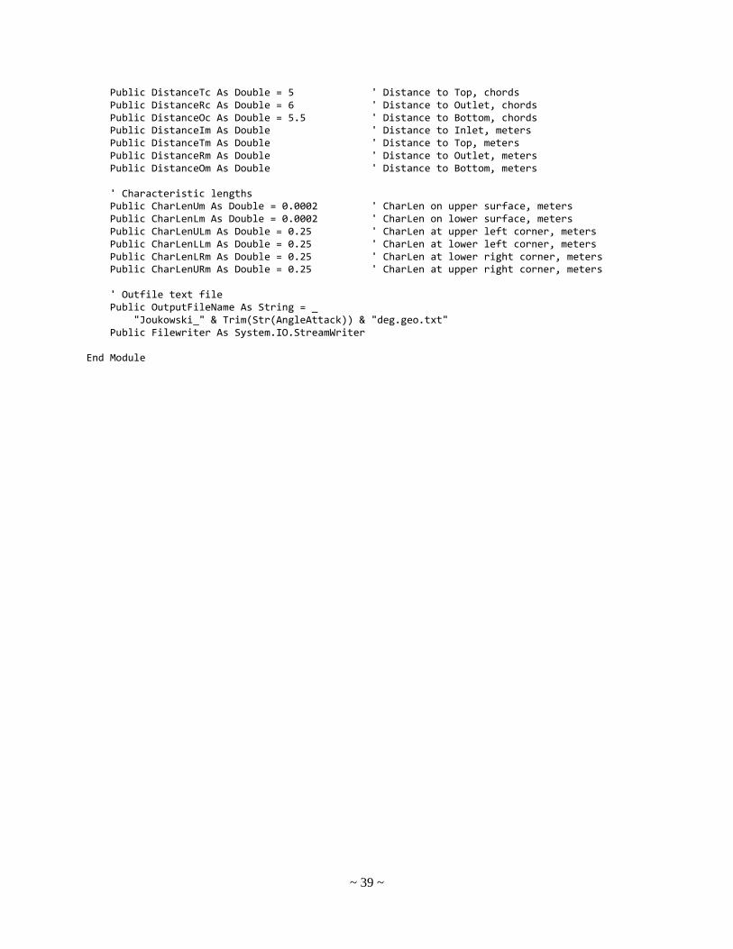
~ 39 ~

Public DistanceTc As Double = 5 ' Distance to Top, chords Public DistanceRc As Double = 6 ' Distance to Outlet, chords Public DistanceOc As Double = 5.5 ' Distance to Bottom, chords Public DistanceIm As Double ' Distance to Inlet, meters Public DistanceTm As Double ' Distance to Top, meters Public DistanceRm As Double ' Distance to Outlet, meters Public DistanceOm As Double ' Distance to Bottom, meters ' Characteristic lengths Public CharLenUm As Double = 0.0002 ' CharLen on upper surface, meters Public CharLenLm As Double = 0.0002 ' CharLen on lower surface, meters Public CharLenULm As Double = 0.25 ' CharLen at upper left corner, meters Public CharLenLLm As Double = 0.25 ' CharLen at lower left corner, meters Public CharLenLRm As Double = 0.25 ' CharLen at lower right corner, meters Public CharLenURm As Double = 0.25 ' CharLen at upper right corner, meters ' Outfile text file Public OutputFileName As String = _ "Joukowski_" & Trim(Str(AngleAttack)) & "deg.geo.txt" Public Filewriter As System.IO.StreamWriter End Module

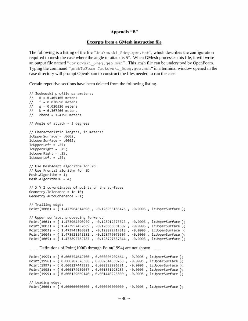
~ 40 ~

Appendix “B”

Excerpts from a GMesh instruction file

The following is a listing of the file “Joukowski_5deg.geo.txt”, which describes the configuration

required to mesh the case where the angle of attack is 5°. When GMesh processes this file, it will write

an output file named “Joukowski_5deg.geo.msh”. This .msh file can be understood by OpenFoam.

Typing the command “gmshToFoam Joukowski_5deg.geo.msh“ in a terminal window opened in the

case directory will prompt OpenFoam to construct the files needed to run the case.

Certain repetitive sections have been deleted from the following listing.

// Joukowski profile parameters: // R = 0.405100 meters // f = 0.030690 meters // g = 0.020320 meters // b = 0.367200 meters // chord = 1.4796 meters // Angle of attack = 5 degrees // Characteristic lengths, in meters: lcUpperSurface = .0002; lcLowerSurface = .0002; lcUpperLeft = .25; lcUpperRight = .25; lcLowerRight = .25; lcLowerLeft = .25; // Use MeshAdapt algorithm for 2D // Use Frontal alorithm for 3D Mesh.Algorithm = 1; Mesh.Algorithm3D = 4; // X Y Z co-ordinates of points on the surface: Geometry.Tolerance = 1e-10; Geometry.AutoCoherence = 1; // Trailing edge: Point(1000) = { 1.473964514698 , -0.128955185476 , -0.0005 , lcUpperSurface }; // Upper surface, proceeding forward: Point(1001) = { 1.473964590959 , -0.128912375523 , -0.0005 , lcUpperSurface }; Point(1002) = { 1.473957457669 , -0.128868381302 , -0.0005 , lcUpperSurface }; Point(1003) = { 1.473943105021 , -0.128822919513 , -0.0005 , lcUpperSurface }; Point(1004) = { 1.473921545181 , -0.128776079507 , -0.0005 , lcUpperSurface }; Point(1005) = { 1.473892782787 , -0.128727857344 , -0.0005 , lcUpperSurface };

.. .. .. Definitions of Point(1006) through Point(1994) are not shown .. .. .. Point(1995) = { 0.000354642700 , 0.003006202664 , -0.0005 , lcUpperSurface }; Point(1996) = { 0.000287376388 , 0.002614558768 , -0.0005 , lcUpperSurface }; Point(1997) = { 0.000227443525 , 0.002222886531 , -0.0005 , lcUpperSurface }; Point(1998) = { 0.000174939037 , 0.001831928283 , -0.0005 , lcUpperSurface }; Point(1999) = { 0.000129669140 , 0.001440225800 , -0.0005 , lcUpperSurface }; // Leading edge: Point(2000) = { 0.000000000000 , 0.000000000000 , -0.0005 , lcUpperSurface };

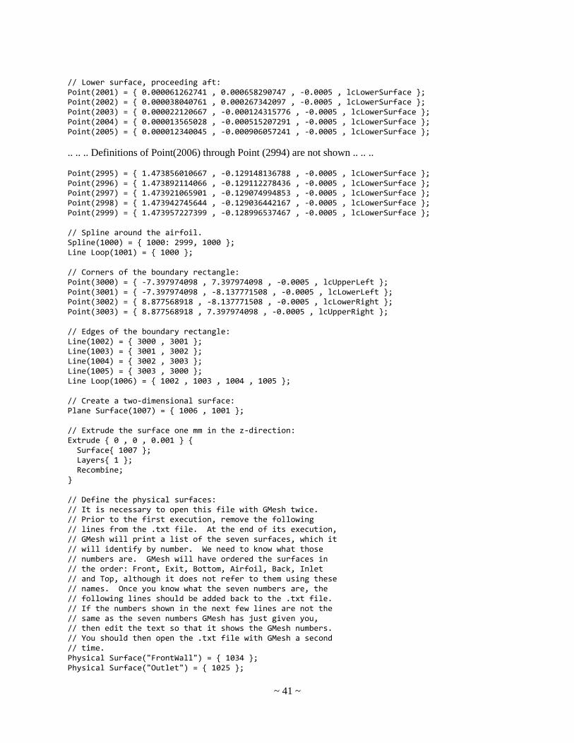
~ 41 ~

// Lower surface, proceeding aft: Point(2001) = { 0.000061262741 , 0.000658290747 , -0.0005 , lcLowerSurface }; Point(2002) = { 0.000038040761 , 0.000267342097 , -0.0005 , lcLowerSurface }; Point(2003) = { 0.000022120667 , -0.000124315776 , -0.0005 , lcLowerSurface }; Point(2004) = { 0.000013565028 , -0.000515207291 , -0.0005 , lcLowerSurface }; Point(2005) = { 0.000012340045 , -0.000906057241 , -0.0005 , lcLowerSurface };

.. .. .. Definitions of Point(2006) through Point (2994) are not shown .. .. .. Point(2995) = { 1.473856010667 , -0.129148136788 , -0.0005 , lcLowerSurface }; Point(2996) = { 1.473892114066 , -0.129112278436 , -0.0005 , lcLowerSurface }; Point(2997) = { 1.473921065901 , -0.129074994853 , -0.0005 , lcLowerSurface }; Point(2998) = { 1.473942745644 , -0.129036442167 , -0.0005 , lcLowerSurface }; Point(2999) = { 1.473957227399 , -0.128996537467 , -0.0005 , lcLowerSurface }; // Spline around the airfoil. Spline(1000) = { 1000: 2999, 1000 }; Line Loop(1001) = { 1000 }; // Corners of the boundary rectangle: Point(3000) = { -7.397974098 , 7.397974098 , -0.0005 , lcUpperLeft }; Point(3001) = { -7.397974098 , -8.137771508 , -0.0005 , lcLowerLeft }; Point(3002) = { 8.877568918 , -8.137771508 , -0.0005 , lcLowerRight }; Point(3003) = { 8.877568918 , 7.397974098 , -0.0005 , lcUpperRight }; // Edges of the boundary rectangle: Line(1002) = { 3000 , 3001 }; Line(1003) = { 3001 , 3002 }; Line(1004) = { 3002 , 3003 }; Line(1005) = { 3003 , 3000 }; Line Loop(1006) = { 1002 , 1003 , 1004 , 1005 }; // Create a two-dimensional surface: Plane Surface(1007) = { 1006 , 1001 }; // Extrude the surface one mm in the z-direction: Extrude { 0 , 0 , 0.001 } { Surface{ 1007 }; Layers{ 1 }; Recombine; } // Define the physical surfaces: // It is necessary to open this file with GMesh twice. // Prior to the first execution, remove the following // lines from the .txt file. At the end of its execution, // GMesh will print a list of the seven surfaces, which it // will identify by number. We need to know what those // numbers are. GMesh will have ordered the surfaces in // the order: Front, Exit, Bottom, Airfoil, Back, Inlet // and Top, although it does not refer to them using these // names. Once you know what the seven numbers are, the // following lines should be added back to the .txt file. // If the numbers shown in the next few lines are not the // same as the seven numbers GMesh has just given you, // then edit the text so that it shows the GMesh numbers. // You should then open the .txt file with GMesh a second // time. Physical Surface("FrontWall") = { 1034 }; Physical Surface("Outlet") = { 1025 };

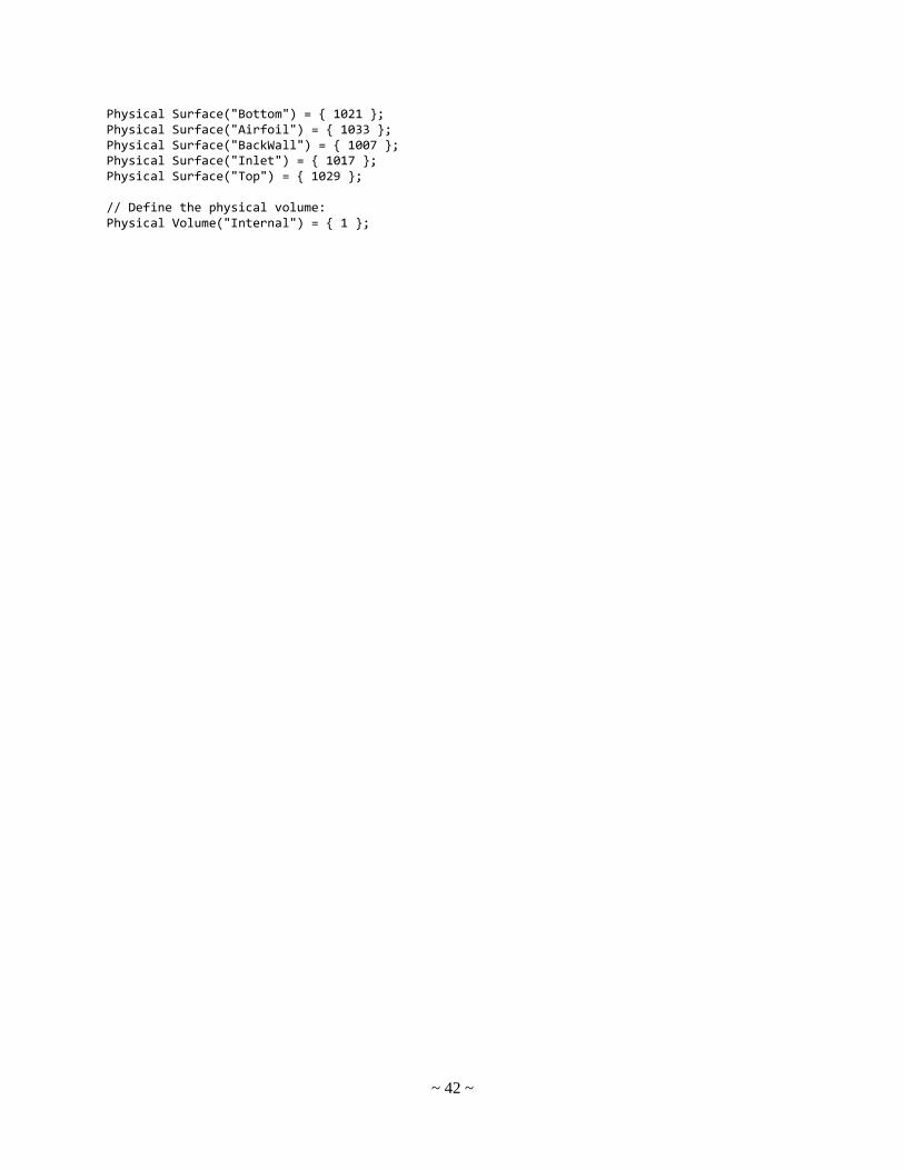
~ 42 ~

Physical Surface("Bottom") = { 1021 }; Physical Surface("Airfoil") = { 1033 }; Physical Surface("BackWall") = { 1007 }; Physical Surface("Inlet") = { 1017 }; Physical Surface("Top") = { 1029 }; // Define the physical volume: Physical Volume("Internal") = { 1 };

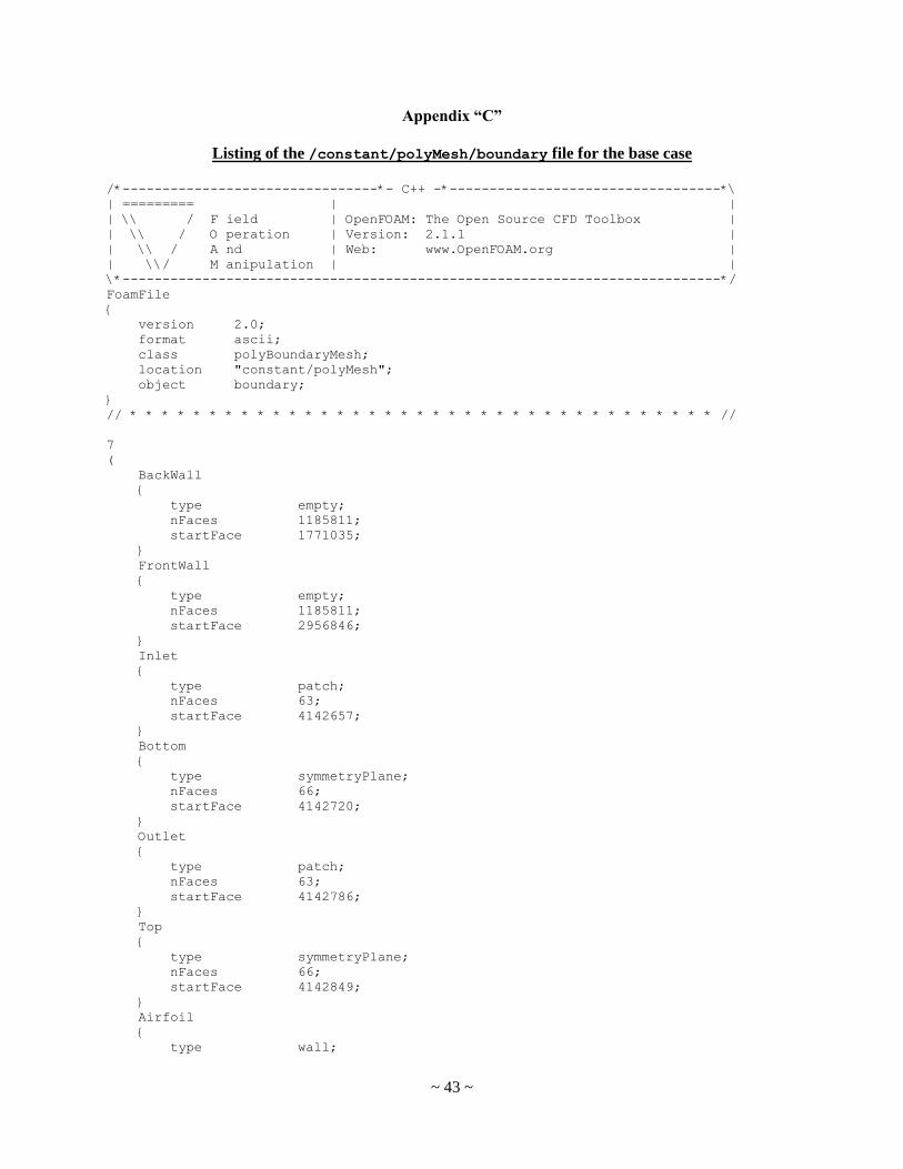
~ 43 ~

Appendix “C”

Listing of the /constant/polyMesh/boundary file for the base case

/*--------------------------------*- C++ -*----------------------------------*\

| ========= | |

| \\ / F ield | OpenFOAM: The Open Source CFD Toolbox |

| \\ / O peration | Version: 2.1.1 |

| \\ / A nd | Web: www.OpenFOAM.org |

| \\/ M anipulation | |

\*---------------------------------------------------------------------------*/

FoamFile

{

version 2.0;

format ascii;

class polyBoundaryMesh;

location "constant/polyMesh";

object boundary;

}

// * * * * * * * * * * * * * * * * * * * * * * * * * * * * * * * * * * * * * //

7

(

BackWall

{

type empty;

nFaces 1185811;

startFace 1771035;

}

FrontWall

{

type empty;

nFaces 1185811;

startFace 2956846;

}

Inlet

{

type patch;

nFaces 63;

startFace 4142657;

}

Bottom

{

type symmetryPlane;

nFaces 66;

startFace 4142720;

}

Outlet

{

type patch;

nFaces 63;

startFace 4142786;

}

Top

{

type symmetryPlane;

nFaces 66;

startFace 4142849;

}

Airfoil

{

type wall;

~ 44 ~

nFaces 15105;

startFace 4142915;

}

)

// ************************************************************************* //

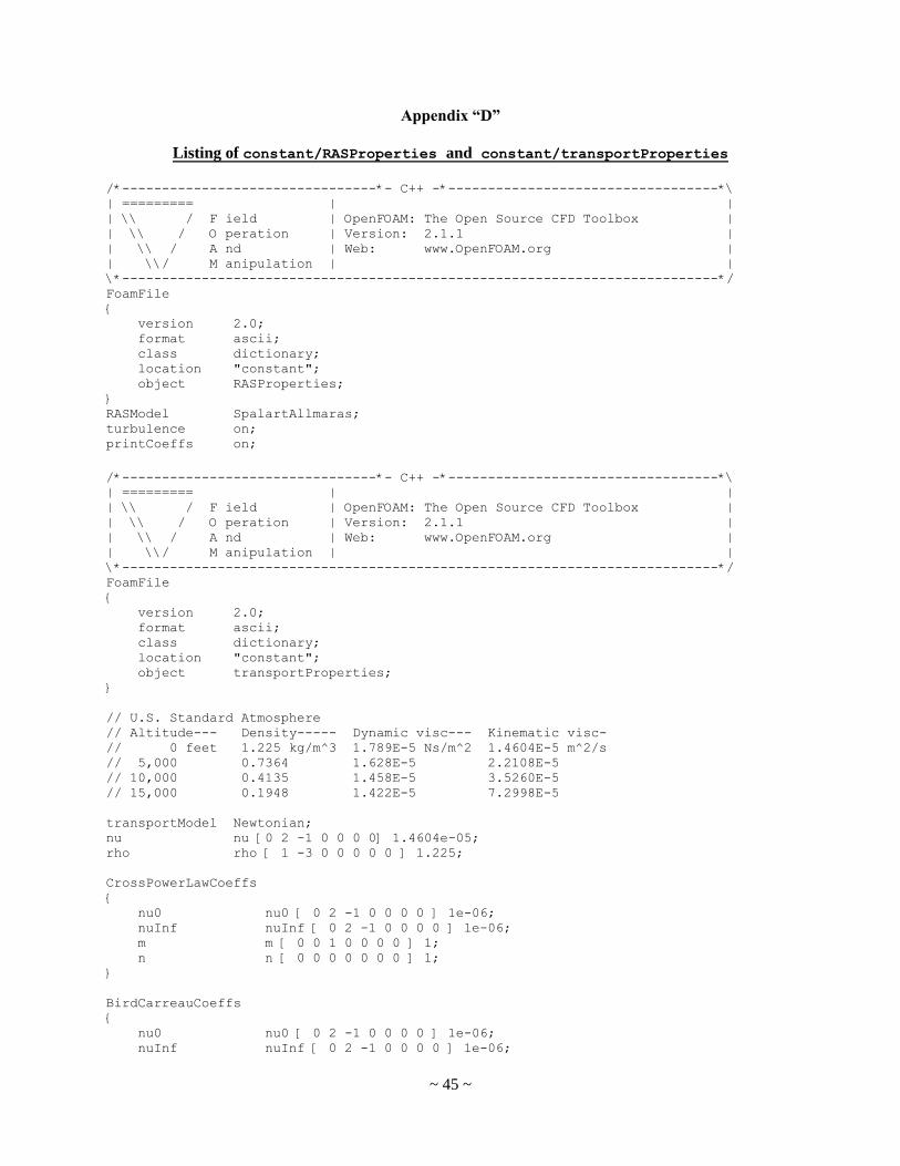
~ 45 ~

Appendix “D”

Listing of constant/RASProperties and constant/transportProperties

/*--------------------------------*- C++ -*----------------------------------*\

| ========= | |

| \\ / F ield | OpenFOAM: The Open Source CFD Toolbox |

| \\ / O peration | Version: 2.1.1 |

| \\ / A nd | Web: www.OpenFOAM.org |

| \\/ M anipulation | |

\*---------------------------------------------------------------------------*/

FoamFile

{

version 2.0;

format ascii;

class dictionary;

location "constant";

object RASProperties;

}

RASModel SpalartAllmaras;

turbulence on;

printCoeffs on;

/*--------------------------------*- C++ -*----------------------------------*\

| ========= | |

| \\ / F ield | OpenFOAM: The Open Source CFD Toolbox |

| \\ / O peration | Version: 2.1.1 |

| \\ / A nd | Web: www.OpenFOAM.org |

| \\/ M anipulation | |

\*---------------------------------------------------------------------------*/

FoamFile

{

version 2.0;

format ascii;

class dictionary;

location "constant";

object transportProperties;

}

// U.S. Standard Atmosphere

// Altitude--- Density----- Dynamic visc--- Kinematic visc-

// 0 feet 1.225 kg/m^3 1.789E-5 Ns/m^2 1.4604E-5 m^2/s

// 5,000 0.7364 1.628E-5 2.2108E-5

// 10,000 0.4135 1.458E-5 3.5260E-5

// 15,000 0.1948 1.422E-5 7.2998E-5

transportModel Newtonian;

nu nu [0 2 -1 0 0 0 0] 1.4604e-05;

rho rho [ 1 -3 0 0 0 0 0 ] 1.225;

CrossPowerLawCoeffs

{

nu0 nu0 [ 0 2 -1 0 0 0 0 ] 1e-06;

nuInf nuInf [ 0 2 -1 0 0 0 0 ] 1e-06;

m m [ 0 0 1 0 0 0 0 ] 1;

n n [ 0 0 0 0 0 0 0 ] 1;

}

BirdCarreauCoeffs

{

nu0 nu0 [ 0 2 -1 0 0 0 0 ] 1e-06;

nuInf nuInf [ 0 2 -1 0 0 0 0 ] 1e-06;

~ 46 ~

k k [ 0 0 1 0 0 0 0 ] 0;

n n [ 0 0 0 0 0 0 0 ] 1;

}

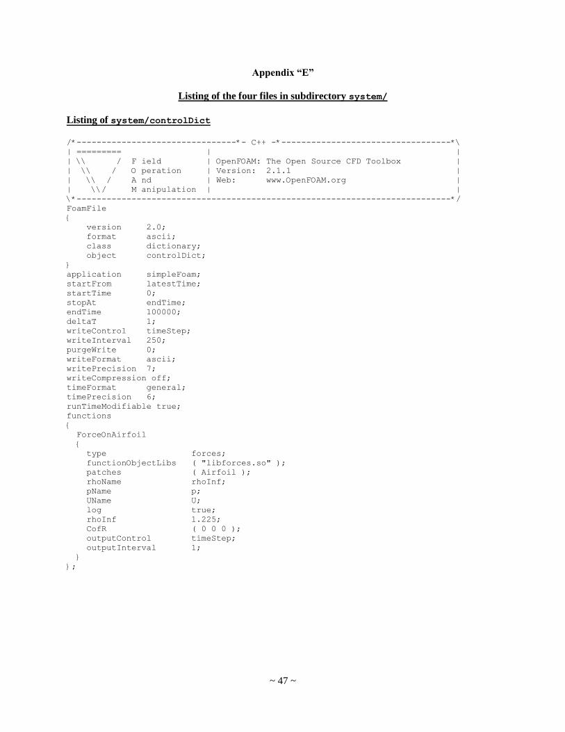
~ 47 ~

Appendix “E”

Listing of the four files in subdirectory system/

Listing of system/controlDict

/*--------------------------------*- C++ -*----------------------------------*\

| ========= | |

| \\ / F ield | OpenFOAM: The Open Source CFD Toolbox |

| \\ / O peration | Version: 2.1.1 |

| \\ / A nd | Web: www.OpenFOAM.org |

| \\/ M anipulation | |

\*---------------------------------------------------------------------------*/

FoamFile

{

version 2.0;

format ascii;

class dictionary;

object controlDict;

}

application simpleFoam;

startFrom latestTime;

startTime 0;

stopAt endTime;

endTime 100000;

deltaT 1;

writeControl timeStep;

writeInterval 250;

purgeWrite 0;

writeFormat ascii;

writePrecision 7;

writeCompression off;

timeFormat general;

timePrecision 6;

runTimeModifiable true;

functions

{

ForceOnAirfoil

{

type forces;

functionObjectLibs ( "libforces.so" );

patches ( Airfoil );

rhoName rhoInf;

pName p;

UName U;

log true;

rhoInf 1.225;

CofR ( 0 0 0 );

outputControl timeStep;

outputInterval 1;

}

};

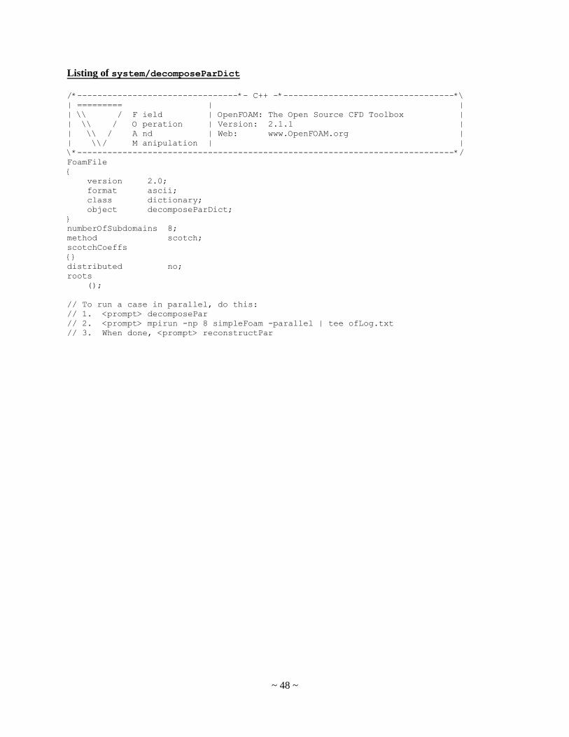
~ 48 ~

Listing of system/decomposeParDict

/*--------------------------------*- C++ -*----------------------------------*\

| ========= | |

| \\ / F ield | OpenFOAM: The Open Source CFD Toolbox |

| \\ / O peration | Version: 2.1.1 |

| \\ / A nd | Web: www.OpenFOAM.org |

| \\/ M anipulation | |

\*---------------------------------------------------------------------------*/

FoamFile

{

version 2.0;

format ascii;

class dictionary;

object decomposeParDict;

}

numberOfSubdomains 8;

method scotch;

scotchCoeffs

{}

distributed no;

roots

();

// To run a case in parallel, do this:

// 1. <prompt> decomposePar

// 2. <prompt> mpirun -np 8 simpleFoam -parallel | tee ofLog.txt

// 3. When done, <prompt> reconstructPar

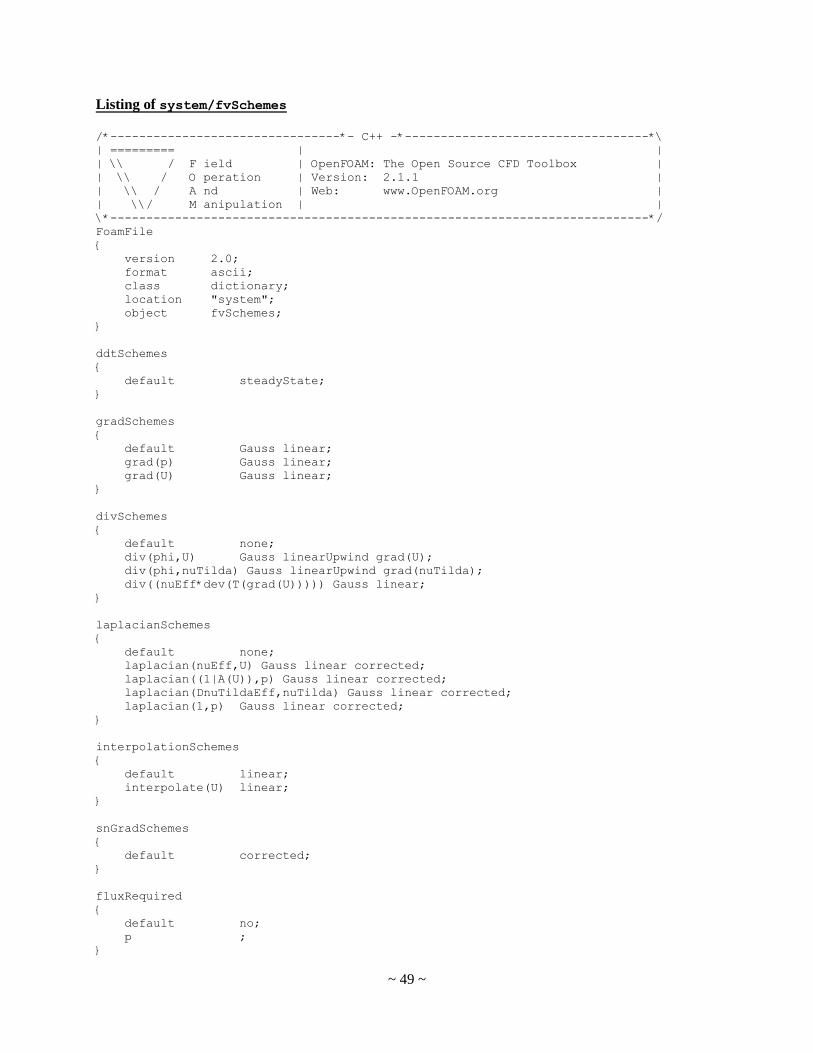
~ 49 ~

Listing of system/fvSchemes

/*--------------------------------*- C++ -*----------------------------------*\

| ========= | |

| \\ / F ield | OpenFOAM: The Open Source CFD Toolbox |

| \\ / O peration | Version: 2.1.1 |

| \\ / A nd | Web: www.OpenFOAM.org |

| \\/ M anipulation | |

\*---------------------------------------------------------------------------*/

FoamFile

{

version 2.0;

format ascii;

class dictionary;

location "system";

object fvSchemes;

}

ddtSchemes

{

default steadyState;

}

gradSchemes

{

default Gauss linear;

grad(p) Gauss linear;

grad(U) Gauss linear;

}

divSchemes

{

default none;

div(phi,U) Gauss linearUpwind grad(U);

div(phi,nuTilda) Gauss linearUpwind grad(nuTilda);

div((nuEff*dev(T(grad(U))))) Gauss linear;

}

laplacianSchemes

{

default none;

laplacian(nuEff,U) Gauss linear corrected;

laplacian((1|A(U)),p) Gauss linear corrected;

laplacian(DnuTildaEff,nuTilda) Gauss linear corrected;

laplacian(1,p) Gauss linear corrected;

}

interpolationSchemes

{

default linear;

interpolate(U) linear;

}

snGradSchemes

{

default corrected;

}

fluxRequired

{

default no;

p ;

}

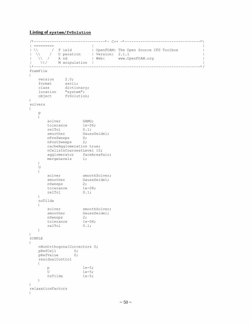
~ 50 ~

Listing of system/fvSolution

/*--------------------------------*- C++ -*----------------------------------*\

| ========= | |

| \\ / F ield | OpenFOAM: The Open Source CFD Toolbox |

| \\ / O peration | Version: 2.1.1 |

| \\ / A nd | Web: www.OpenFOAM.org |

| \\/ M anipulation | |

\*---------------------------------------------------------------------------*/

FoamFile

{

version 2.0;

format ascii;

class dictionary;

location "system";

object fvSolution;

}

solvers

{

p

{

solver GAMG;

tolerance 1e-06;

relTol 0.1;

smoother GaussSeidel;

nPreSweeps 0;

nPostSweeps 2;

cacheAgglomeration true;

nCellsInCoarsestLevel 10;

agglomerator faceAreaPair;

mergeLevels 1;

}

U

{

solver smoothSolver;

smoother GaussSeidel;

nSweeps 2;

tolerance 1e-08;

relTol 0.1;

}

nuTilda

{

solver smoothSolver;

smoother GaussSeidel;

nSweeps 2;

tolerance 1e-08;

relTol 0.1;

}

}

SIMPLE

{

nNonOrthogonalCorrectors 0;

pRefCell 0;

pRefValue 0;

residualControl

{

p 1e-5;

U 1e-5;

nuTilda 1e-5;

}

}

relaxationFactors

{

~ 51 ~

fields

{

p 0.35;

}

equations

{

U 0.65;

nuTilda 0.8;

}

}

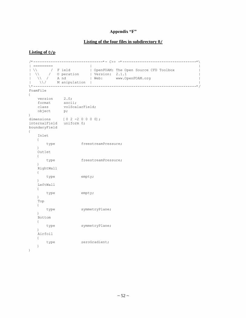
~ 52 ~

Appendix “F”

Listing of the four files in subdirectory 0/

Listing of 0/p

/*--------------------------------*- C++ -*----------------------------------*\

| ========= | |

| \\ / F ield | OpenFOAM: The Open Source CFD Toolbox |

| \\ / O peration | Version: 2.1.1 |

| \\ / A nd | Web: www.OpenFOAM.org |

| \\/ M anipulation | |

\*---------------------------------------------------------------------------*/

FoamFile

{

version 2.0;

format ascii;

class volScalarField;

object p;

}

dimensions [0 2 -2 0 0 0 0];

internalField uniform 0;

boundaryField

{

Inlet

{

type freestreamPressure;

}

Outlet

{

type freestreamPressure;

}

RightWall

{

type empty;

}

LeftWall

{

type empty;

}

Top

{

type symmetryPlane;

}

Bottom

{

type symmetryPlane;

}

Airfoil

{

type zeroGradient;

}

}

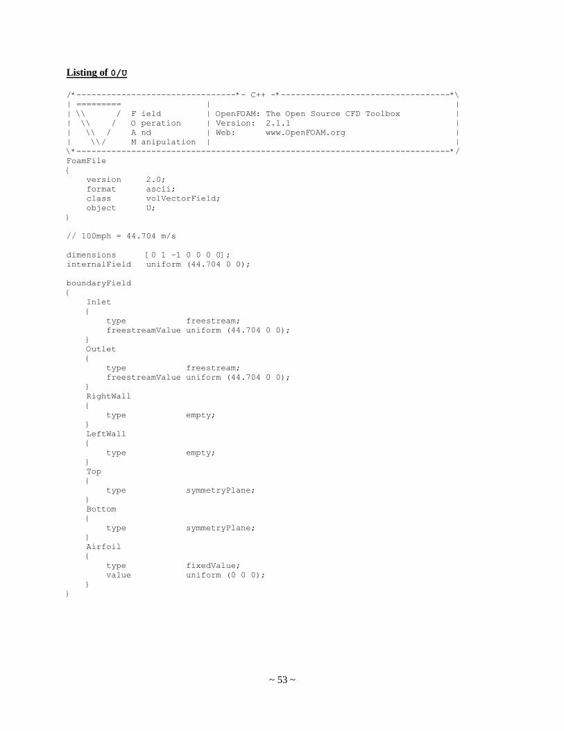
~ 53 ~

Listing of 0/U

/*--------------------------------*- C++ -*----------------------------------*\

| ========= | |

| \\ / F ield | OpenFOAM: The Open Source CFD Toolbox |

| \\ / O peration | Version: 2.1.1 |

| \\ / A nd | Web: www.OpenFOAM.org |

| \\/ M anipulation | |

\*---------------------------------------------------------------------------*/

FoamFile

{

version 2.0;

format ascii;

class volVectorField;

object U;

}

// 100mph = 44.704 m/s

dimensions [0 1 -1 0 0 0 0];

internalField uniform (44.704 0 0);

boundaryField

{

Inlet

{

type freestream;

freestreamValue uniform (44.704 0 0);

}

Outlet

{

type freestream;

freestreamValue uniform (44.704 0 0);

}

RightWall

{

type empty;

}

LeftWall

{

type empty;

}

Top

{

type symmetryPlane;

}

Bottom

{

type symmetryPlane;

}

Airfoil

{

type fixedValue;

value uniform (0 0 0);

}

}

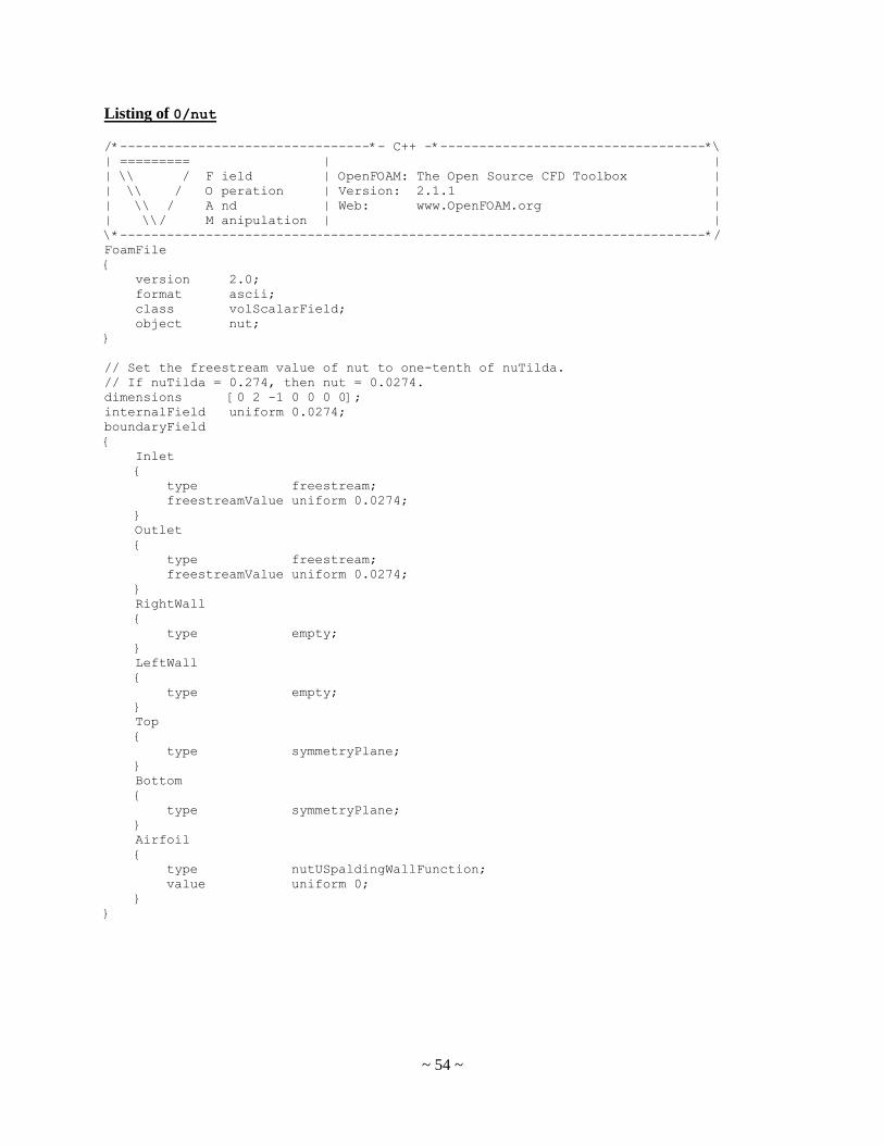
~ 54 ~

Listing of 0/nut

/*--------------------------------*- C++ -*----------------------------------*\

| ========= | |

| \\ / F ield | OpenFOAM: The Open Source CFD Toolbox |

| \\ / O peration | Version: 2.1.1 |

| \\ / A nd | Web: www.OpenFOAM.org |

| \\/ M anipulation | |

\*---------------------------------------------------------------------------*/

FoamFile

{

version 2.0;

format ascii;

class volScalarField;

object nut;

}

// Set the freestream value of nut to one-tenth of nuTilda.

// If nuTilda = 0.274, then nut = 0.0274.

dimensions [0 2 -1 0 0 0 0];

internalField uniform 0.0274;

boundaryField

{

Inlet

{

type freestream;

freestreamValue uniform 0.0274;

}

Outlet

{

type freestream;

freestreamValue uniform 0.0274;

}

RightWall

{

type empty;

}

LeftWall

{

type empty;

}

Top

{

type symmetryPlane;

}

Bottom

{

type symmetryPlane;

}

Airfoil

{

type nutUSpaldingWallFunction;

value uniform 0;

}

}

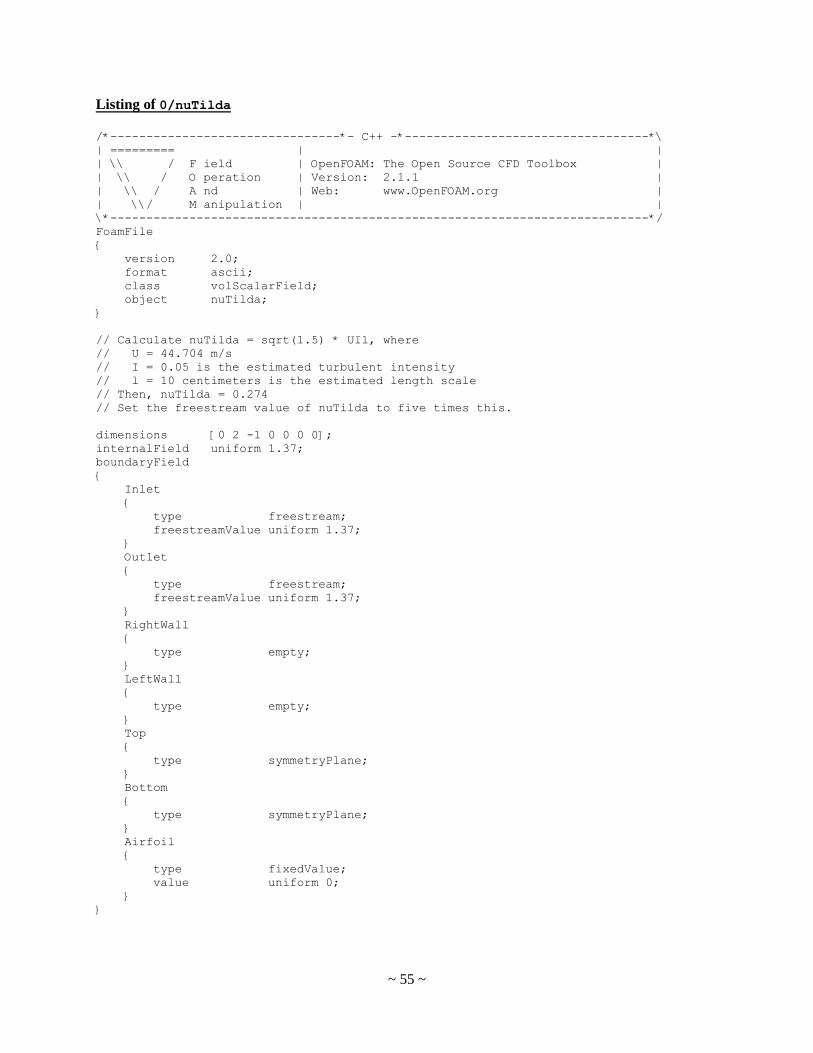
~ 55 ~

Listing of 0/nuTilda

/*--------------------------------*- C++ -*----------------------------------*\

| ========= | |

| \\ / F ield | OpenFOAM: The Open Source CFD Toolbox |

| \\ / O peration | Version: 2.1.1 |

| \\ / A nd | Web: www.OpenFOAM.org |

| \\/ M anipulation | |

\*---------------------------------------------------------------------------*/

FoamFile

{

version 2.0;

format ascii;

class volScalarField;

object nuTilda;

}

// Calculate nuTilda = sqrt(1.5) * UIl, where

// U = 44.704 m/s

// I = 0.05 is the estimated turbulent intensity

// l = 10 centimeters is the estimated length scale

// Then, nuTilda = 0.274

// Set the freestream value of nuTilda to five times this.

dimensions [0 2 -1 0 0 0 0];

internalField uniform 1.37;

boundaryField

{

Inlet

{

type freestream;

freestreamValue uniform 1.37;

}

Outlet

{

type freestream;

freestreamValue uniform 1.37;

}

RightWall

{

type empty;

}

LeftWall

{

type empty;

}

Top

{

type symmetryPlane;

}

Bottom

{

type symmetryPlane;

}

Airfoil

{

type fixedValue;

value uniform 0;

}

}