1

Joseph-Louis Lagrange (1736-1813) Charles Hermite (1822-1901)

Summary of Lagrange/Hermite Interpolation1) Find a “good” polynomial basis

Ø Lagrange Basis: 𝐿",$(𝑥)Ø (Newton) Divided-difference basis:

𝑥 − 𝑥) … (𝑥 − 𝑥$+,)ØHermite Basis: 𝐻",$ 𝑥 , .𝐻",$ 𝑥Ø (Newton) Divided-difference basis for Hermite:

𝑥 − 𝑧) … 𝑥 − 𝑧$+,2) Interpolation formula

𝑃" 𝑥 = 2$3)

"

𝑓(𝑥$)𝐿",$(𝑥)

𝐻" 𝑥 = 2$3)

"

𝑓 𝑥$ 𝐻",$ 𝑥 +2$3)

"

𝑓′ 𝑥$ .𝐻",$ 𝑥

2

3

Joseph-Louis Lagrange (1736-1813) Sir Isaac Newton (1642-1726)

Lagrange form V.S. Newton form

4

https://en.wikipedia.org/wiki/Newton_polynomial

Quoted from wiki:

Lagrange is sometimes said to require less work, and is sometimes recommended for problems in which it's known, in advance, from previous experience, how many terms are needed for sufficient accuracy.

The divided difference methods have the advantage that more data points can be added, for improved accuracy, without re-doing the whole problem. The terms based on the previous data points can continue to be used. With the ordinary Lagrange formula, to do the problem with more data points would require re-doing the whole problem.…..

3.5 Cubic Spline Interpolation

5

Problems with High Order Polynomial Interpolation

• 20th degree Lagrange interpolant for

𝑓 𝑥 = ,,789:;

on the interval [-1,1] using 21 equal-spaced nodes. • The Lagrange interpolating polynomial oscillates

between interpolation points. [Runge’s phenomenon]6

-1 -0.5 0 0.5 1

0

0.2

0.4

0.6

0.8

1

Remedy 1: use non-uniform nodes

• 20th degree Lagrange interpolant for

𝑓 𝑥 = ,,789:;

on the interval [-1,1] using n=21 Chebyshev nodes:

𝑥$ = −cos𝑘𝜋𝑛, 𝑘 = 0,… , 𝑛

7

-1 -0.5 0 0.5 1

0

0.2

0.4

0.6

0.8

1

8

% function and interpolation nodesf = @(x) 1./(1+25*x.*x);n = 21; % degree 20 interpolation%xNodes = linspace(-1,1,n+1);xNodes = -cos([0:n]/n*pi); % chebyshev nodesyNodes = f(xNodes);

% evaluate function at 1001 uniform pointsm = 1001;xGrid = linspace(-1,1,m);pGrid = zeros(size(xGrid));

for k = 0:n yk = yNodes(k+1); phi_k = lagrange_basis(xGrid, xNodes, k); % k-th basis eval @ xGrid pGrid = pGrid + yk*phi_k;end

plot(xGrid, f(xGrid),'b', xGrid, pGrid, 'r', xNodes, yNodes, 'ko',... 'LineWidth', 4,'MarkerSize',10)set(gca, 'FontSize',24)axis([-1,1,-0.1,1.1])shgsaveas(gcf, 'cheb.eps','epsc')%saveas(gcf, 'uniform.eps','epsc')

1

lagrange_interp_cheby.mscript .m file for Lagrange interp. with Cheb. nodes

Remedy 2: use smooth piecewise polynomials

• n=21 equal-spaced interpolation nodes

𝑥$ = −1 +2𝑘𝑛, 𝑘 = 0,… , 𝑛

• On each small interval [𝑥F, 𝑥F7,], 𝑆(𝑥) is a polynomial of degree 3

• 𝑆(𝑥) has continuous first and second derivatives at internal nodes 𝑥F for 𝑗 = 1,… , 𝑛 − 1 9

(smooth) piecewise polynomial interpolation [splines]

10

• Spline: A spline consists of a long strip of wood (a lath) fixed in position at a number of points. The lath will take the shape which minimizes the energy required for bending it between the fixed points, and thus adopt the smoothest possible shape.

Cubic Splines• Idea: Use piecewise polynomial interpolation, i.e,

divide the interval into smaller sub-intervals, and construct different low degree polynomial approximations (with small oscillations) on the sub-intervals.

11

Example. Piecewise-linear interpolation

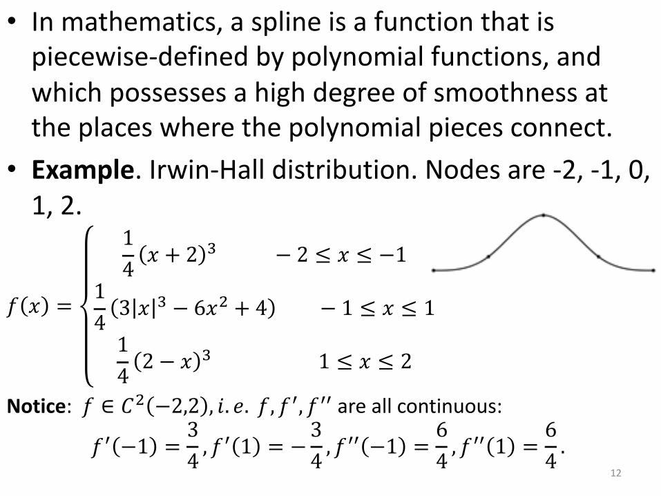
• In mathematics, a spline is a function that is piecewise-defined by polynomial functions, and which possesses a high degree of smoothness at the places where the polynomial pieces connect.

• Example. Irwin-Hall distribution. Nodes are -2, -1, 0, 1, 2.

𝑓 𝑥 =

14𝑥 + 2 K − 2 ≤ 𝑥 ≤ −1

143 𝑥 K − 6𝑥8 + 4 − 1 ≤ 𝑥 ≤ 1142 − 𝑥 K 1 ≤ 𝑥 ≤ 2

Notice: 𝑓 ∈ 𝐶8 −2,2 , 𝑖. 𝑒. 𝑓, 𝑓T, 𝑓TT are all continuous:

𝑓T −1 =34, 𝑓T 1 = −

34, 𝑓TT −1 =

64, 𝑓TT 1 =

64.

12

cubic spline interpolation is a piecewise-polynomial approximation thata) use cubic polynomials between each successive

pair of nodes.b) has both continuous first and second derivatives

at the internal nodes

13

Definition 3.10. Given a function 𝑓 on [𝑎, 𝑏] and nodes 𝑎 =𝑥) < ⋯ < 𝑥" = 𝑏, a cubic spline interpolant 𝑆 for 𝑓 satisfies:(a) 𝑆(𝑥) is a cubic polynomial 𝑆F(𝑥) on [𝑥F, 𝑥F7,] with:

𝑆F 𝑥 = 𝑎F + 𝑏F 𝑥 − 𝑥F + 𝑐F 𝑥 − 𝑥F8 + 𝑑F 𝑥 − 𝑥F

K

∀𝑗 = 0,1, … , 𝑛 − 1.(b) [interpolation property]

𝑆F 𝑥F = 𝑓(𝑥F) and 𝑆F 𝑥F7, = 𝑓 𝑥F7, , ∀𝑗 = 0,1, … , 𝑛 − 1.(c) [continuous first derivative]

𝑆TF 𝑥F7, = 𝑆TF7, 𝑥F7, , ∀𝑗 = 0,1, … , 𝑛 − 2.(d) [continuous second derivative]

𝑆TTF 𝑥F7, = 𝑆TTF7, 𝑥F7, , ∀𝑗 = 0,1, … , 𝑛 − 2.(e) [One of the following boundary conditions]:(i) 𝑆TT 𝑥) = 𝑆TT 𝑥" = 0 (called free or natural boundary)(ii) 𝑆T 𝑥) = 𝑓′(𝑥)) and 𝑆T 𝑥" = 𝑓′(𝑥") (called clamped

boundary) 14

The spline segment 𝑆F(𝑥) is on 𝑥F, 𝑥F7, . The spline segment 𝑆F7,(𝑥) is on 𝑥F7,, 𝑥F78 . Things to match at interior point 𝑥F7,:• Their function values: 𝑆F 𝑥F7, = 𝑆F7, 𝑥F7, =𝑓 𝑥F7,

• First derivative values: 𝑆TF 𝑥F7, = 𝑆TF7, 𝑥F7,• Second derivative values: 𝑆TTF 𝑥F7, = 𝑆TTF7, 𝑥F7,

15

The Cubic spline interpolation problemGiven data 𝑥), 𝑓 𝑥) , … , (𝑥", 𝑓 𝑥" ), find the coefficients 𝑎F, 𝑏F, 𝑐F, 𝑑F for 𝑗 = 0,… , 𝑛 − 1 of the Cubic spline interpolant 𝑆 𝑥 :

𝑆 𝑥 =

𝑆) 𝑥 𝑥) ≤ 𝑥 ≤ 𝑥,

… …𝑆F(𝑥) 𝑥F ≤ 𝑥 ≤ 𝑥F7,

… …𝑆"+,(𝑥) 𝑥"+, ≤ 𝑥 ≤ 𝑥"

Where 𝑆F 𝑥 = 𝑎F + 𝑏F 𝑥 − 𝑥F + 𝑐F 𝑥 − 𝑥F8 + 𝑑F 𝑥 − 𝑥F

K,

such that conditions in (b)-(e) of Definition 3.10holds.

16

Example 1. Construct a natural cubic spline 𝑆 𝑥through (1,2), (2,3) and (3,5).

17

Building Cubic Splines• Define: 𝑆F 𝑥 = 𝑎F + 𝑏F 𝑥 − 𝑥F + 𝑐F(𝑥 − 𝑥F)8+𝑑F(𝑥 − 𝑥F)K

and ℎF = 𝑥F7, − 𝑥F, ∀𝑗 = 0,1, … , (𝑛 − 1).• Also define 𝑎" = 𝑓 𝑥" ; 𝑏" = 𝑆T 𝑥" ; 𝑐" = 𝑆TT(𝑥")/2.From Definition 3.10:1) 𝑆F 𝑥F = 𝑎F = 𝑓 𝑥F for 𝑗 = 0,1, … , (𝑛 − 1).2) 𝑆F 𝑥F7, = 𝑎F7, = 𝑎F + 𝑏FℎF + 𝑐F(ℎF )8+𝑑F(ℎF )K

for 𝑗 = 0,1, … , (𝑛 − 1).

3) 𝑆TF 𝑥F = 𝑆TF7, 𝑥F : 𝑏F7, = 𝑏F + 2𝑐FℎF + 3𝑑F(ℎF )8for 𝑗 = 0,1, … , (𝑛 − 1).

4) 𝑆TTF 𝑥F = 𝑆TTF7, 𝑥F : 𝑐F7, = 𝑐F + 3𝑑FℎFfor 𝑗 = 0,1, … , 𝑛 − 1 .

5) Natural or clamped boundary conditions18

Solve 𝑎F, 𝑏F, 𝑐F, 𝑑F by substitution:1. Solve Eq. 4) for 𝑑F =

cdef+cdKgd

(3.17) , and substitute into Eqs. 2) and 3) to get:

2. 𝑎F7, = 𝑎F + 𝑏FℎF +gd;

K2𝑐F + 𝑐F7, ; (3.18)

𝑏F7, = 𝑏F + ℎF 𝑐F + 𝑐F7, . (3.19)3. Solve for 𝑏F in Eq. (3.18) to get:

𝑏F =,gd

𝑎F7, − 𝑎F − gdK2𝑐F + 𝑐F7, . (3.20)

Reduce the index by 1 to get:

𝑏F+, =,

gdjf𝑎F − 𝑎F+, −

gdjfK

2𝑐F+, + 𝑐F .

4. Substitute 𝑏F and 𝑏F+, into Eq. (3.19) [reduce index by 1]:ℎF+,𝑐F+, + 2 ℎF+, + ℎF 𝑐F + ℎF𝑐F7, = (3.21)

3ℎF

𝑎F7, − 𝑎F −3ℎF+,

(𝑎F − 𝑎F+,)

for 𝑗 = 1,2, … , 𝑛 − 1 . 19

Solving the Resulting Equations for 𝑐∀𝑗 = 1,2, … , (𝑛 − 1)

ℎF+,𝑐F+, + 2 ℎF+, + ℎF 𝑐F + ℎF𝑐F7,

=3ℎF

𝑎F7, − 𝑎F −3ℎF+,

𝑎F − 𝑎F+, (3.21)

Remark: (n-1) equations for (n+1) unknowns {𝑐F}F3)" . Eq. (3.21) is solved with boundary conditions. • Once compute 𝑐F, we then compute:

𝑏F =mdef+md

gd− gd 8cd7cdef

K(3.20)

and

𝑑F =cdef+cdKgd

(3.17) for 𝑗 = 0,1,2, … , (𝑛 − 1)20

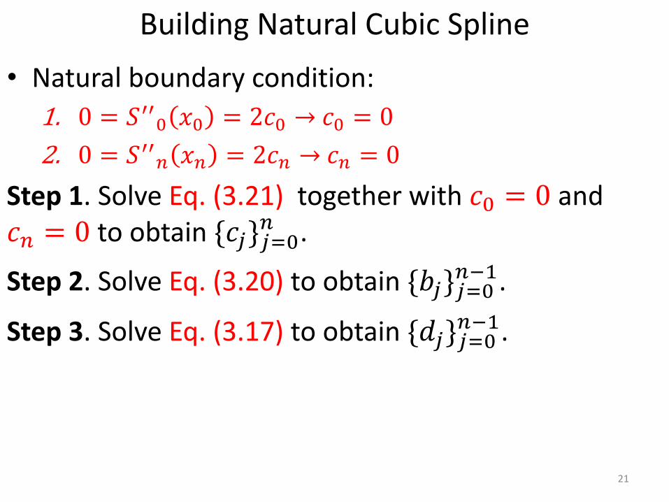
Building Natural Cubic Spline • Natural boundary condition: 1. 0 = 𝑆TT) 𝑥) = 2𝑐) → 𝑐) = 02. 0 = 𝑆TT" 𝑥" = 2𝑐" → 𝑐" = 0

Step 1. Solve Eq. (3.21) together with 𝑐) = 0 and 𝑐" = 0 to obtain {𝑐F}F3)" .

Step 2. Solve Eq. (3.20) to obtain {𝑏F}F3)"+,.

Step 3. Solve Eq. (3.17) to obtain {𝑑F}F3)"+,.

21

Building Natural Cubic Spline • Natural boundary condition: 1. 0 = 𝑆TT) 𝑥) = 2𝑐) → 𝑐) = 02. 0 = 𝑆TT" 𝑥" = 2𝑐" → 𝑐" = 0

Step 1. Solve Eq. (3.21) together with 𝑐) = 0 and 𝑐" = 0 to obtain {𝑐F}F3)" .

Step 2. Solve Eq. (3.20) to obtain {𝑏F}F3)"+,.

Step 3. Solve Eq. (3.17) to obtain {𝑑F}F3)"+,.

22

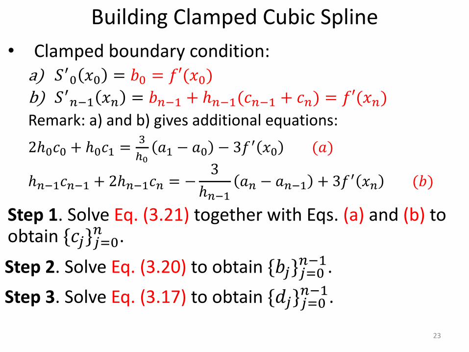
Building Clamped Cubic Spline• Clamped boundary condition: a) 𝑆T) 𝑥) = 𝑏) = 𝑓′(𝑥))b) 𝑆T"+, 𝑥" = 𝑏"+, + ℎ"+,(𝑐"+, + 𝑐") = 𝑓′(𝑥")Remark: a) and b) gives additional equations:2ℎ)𝑐) + ℎ)𝑐, =

Kgq

𝑎, − 𝑎) − 3𝑓T 𝑥) (𝑎)

ℎ"+,𝑐"+, + 2ℎ"+,𝑐" = −3

ℎ"+,𝑎" − 𝑎"+, + 3𝑓T 𝑥" (𝑏)

Step 1. Solve Eq. (3.21) together with Eqs. (a) and (b) to obtain {𝑐F}F3)" .Step 2. Solve Eq. (3.20) to obtain {𝑏F}F3)"+,.Step 3. Solve Eq. (3.17) to obtain {𝑑F}F3)"+,.

23

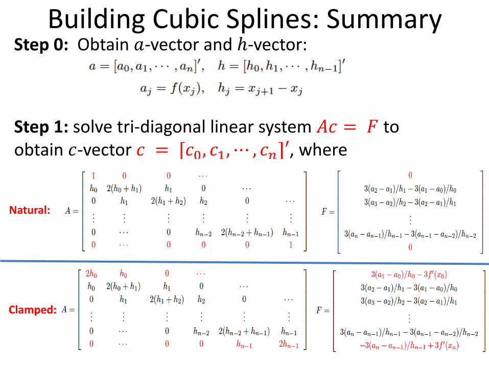
Building Cubic Splines: SummaryStep 0: Obtain 𝑎-vector and ℎ-vector:

Step 1: solve tri-diagonal linear system 𝐴𝑐 = 𝐹 to obtain 𝑐-vector 𝑐 = [𝑐), 𝑐,,⋯ , 𝑐"]′, where

24

Natural:

Clamped:

Step 2: Recover 𝑏-vector 𝑏 = [𝑏), 𝑏,,⋯ , 𝑏"+,]′:

𝑏F =mdef+md

gd−

gd 8cd7cdefK

(3.20)

Step 3: Recover 𝑑-vector 𝑑 = [𝑑), 𝑑,,⋯ , 𝑑"+,]′:

𝑑F =cdef+cdKgd

(3.17)

Building Cubic Splines: Summary

25

Remark: Main computational cost is the linear system solve in Step 1. In MATLAB, we simply use the “backslash” \command to solve the system:

𝑐 = 𝐴\F;

Example 2. (MATLAB) Use data points (0,1), (1, 𝑒), (2, 𝑒8), (3, 𝑒K) to form a) a natural cubic spline 𝑆 𝑥 that approximates 𝑓 𝑥 = 𝑒:.

b) a clamped cubic spline 𝑆 𝑥 that approximates 𝑓 𝑥 = 𝑒: with derivative information 𝑓’(0) =1, 𝑓’(3) = 𝑒K.

26

27

% input: data pointsf = @(x) exp(x);xNodes = [0:3]'; % column vectoryNodes = f(xNodes);

%--- STEP 0: obtain the a-vectora = yNodes;

%--- STEP 1: form linear system, solve for c-vectorn = length(xNodes)-1;% mesh size, vector of size nh = xNodes(2:n+1)-xNodes(1:n);% form the matrixA = zeros(n+1,n+1);A(1,1) =1;for j = 2:n A(j,j-1) = h(j-1); A(j,j) = 2*(h(j-1)+h(j)); A(j,j+1) = h(j);endA(n+1,n+1)=1;% form the right hand sideF = zeros(n+1,1);for j = 2:n F(j) = 3/h(j)*(a(j+1)-a(j))... - 3/h(j-1)*(a(j)-a(j-1));end

% solve for c [backslash]c = A\F;

%--- STEP 2: solve for b-vectorb = zeros(n,1);for j = 1:n b(j) = 1/h(j)*(a(j+1)-a(j))... -h(j)/3*(2*c(j)+c(j+1));end

%--- STEP 3: solve for d-vectord = zeros(n,1);for j=1:n d(j) = (c(j+1)-c(j))/3/h(j);end

%--- STEP 4: plot solution% loop over subintervalsxGrid = []; sGrid = [];for j = 1:n x0 = xNodes(j); x1 = xNodes(j+1); xTemp = linspace(x0,x1,20); sTemp = a(j)+b(j)*(xTemp-x0)+c(j)*(xTemp-x0).^2+d(j)*(xTemp-x0).^3;

1

% input: data pointsf = @(x) exp(x);xNodes = [0:3]'; % column vectoryNodes = f(xNodes);

%--- STEP 0: obtain the a-vectora = yNodes;

%--- STEP 1: form linear system, solve for c-vectorn = length(xNodes)-1;% mesh size, vector of size nh = xNodes(2:n+1)-xNodes(1:n);% form the matrixA = zeros(n+1,n+1);A(1,1) =1;for j = 2:n A(j,j-1) = h(j-1); A(j,j) = 2*(h(j-1)+h(j)); A(j,j+1) = h(j);endA(n+1,n+1)=1;% form the right hand sideF = zeros(n+1,1);for j = 2:n F(j) = 3/h(j)*(a(j+1)-a(j))... - 3/h(j-1)*(a(j)-a(j-1));end

% solve for c [backslash]c = A\F;

%--- STEP 2: solve for b-vectorb = zeros(n,1);for j = 1:n b(j) = 1/h(j)*(a(j+1)-a(j))... -h(j)/3*(2*c(j)+c(j+1));end

%--- STEP 3: solve for d-vectord = zeros(n,1);for j=1:n d(j) = (c(j+1)-c(j))/3/h(j);end

%--- STEP 4: plot solution% loop over subintervalsxGrid = []; sGrid = [];for j = 1:n x0 = xNodes(j); x1 = xNodes(j+1); xTemp = linspace(x0,x1,20); sTemp = a(j)+b(j)*(xTemp-x0)+c(j)*(xTemp-x0).^2+d(j)*(xTemp-x0).^3;

1

natural cubic spline (script .m file)natural_cubic_spline.m

xGrid = [xGrid, xTemp]; sGrid = [sGrid, sTemp];endplot(xGrid, f(xGrid),'b', xGrid, sGrid, 'r', xNodes, yNodes, 'ko',... 'LineWidth', 4,'MarkerSize',10)legend('F(x)', 'S(x)','Nodes','Location','best')set(gca, 'FontSize', 24)

Published with MATLAB® R2019a

2

28

natural cubic spline (script .m file continued)natural_cubic_spline.m

%--- STEP 4: plot solution% loop over subintervalsxGrid = []; sGrid = [];for j = 1:n x0 = xNodes(j); x1 = xNodes(j+1); xTemp = linspace(x0,x1,20); sTemp = a(j)+b(j)*(xTemp-x0)... +c(j)*(xTemp-x0).^2+d(j)*(xTemp-x0).^3; xGrid = [xGrid, xTemp]; sGrid = [sGrid, sTemp];endplot(xGrid, f(xGrid),'b', ... xGrid, sGrid, 'r', ... xNodes, yNodes, 'ko',... 'LineWidth', 4,'MarkerSize',10)legend('F(x)', 'S(x)','Nodes','Location','best')set(gca, 'FontSize', 24)

Published with MATLAB® R2019a

1

****clamped cubic spline code is given in course webpage

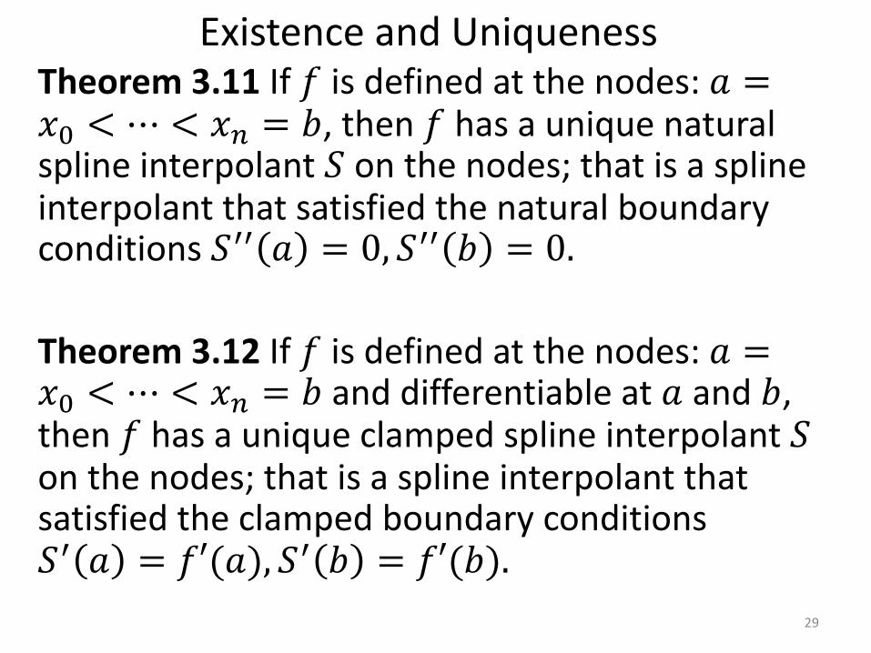
Theorem 3.11 If 𝑓 is defined at the nodes: 𝑎 =𝑥) < ⋯ < 𝑥" = 𝑏, then 𝑓 has a unique natural spline interpolant 𝑆 on the nodes; that is a spline interpolant that satisfied the natural boundary conditions 𝑆TT 𝑎 = 0, 𝑆TT 𝑏 = 0.

Theorem 3.12 If 𝑓 is defined at the nodes: 𝑎 =𝑥) < ⋯ < 𝑥" = 𝑏 and differentiable at 𝑎 and 𝑏, then 𝑓 has a unique clamped spline interpolant 𝑆on the nodes; that is a spline interpolant that satisfied the clamped boundary conditions 𝑆T 𝑎 = 𝑓′(𝑎), 𝑆T 𝑏 = 𝑓′(𝑏).

29

Existence and Uniqueness

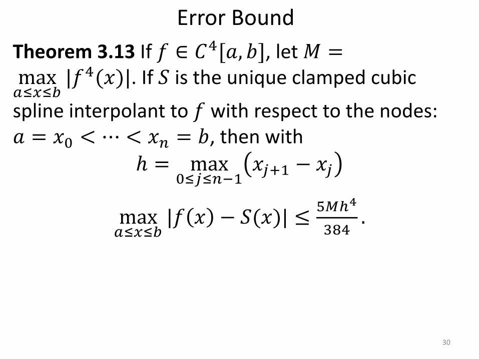
Error BoundTheorem 3.13 If 𝑓 ∈ 𝐶w[𝑎, 𝑏], let 𝑀 =maxm{:{|

|𝑓w(𝑥)|. If 𝑆 is the unique clamped cubic spline interpolant to 𝑓 with respect to the nodes: 𝑎 = 𝑥) < ⋯ < 𝑥" = 𝑏, then with

ℎ = max){F{"+,

𝑥F7, − 𝑥F

maxm{:{|

|𝑓 𝑥 − 𝑆(𝑥)| ≤ 9~g�

K�w.

30