Jordan University of Science & Technology

Department of Electrical Engineering

Digital Signal Processing Laboratory

Using

TMS320C6713 DSP Starter Kit

(EE462)

2

PREFACE This Booklet contains a selected and edited laboratory experiments that were taken with some minor modifications from the book “Digital Signal Processing and Applications with the TMS320C6713 and TMS320C6416 DSK”, second edition, john Wiley & Sons, 2008 written by Rulph Chassaing and Donald Reay. The book has a wide variety of digital signal processing and filter design experiments that can be run on the TMS320C6713 and TMS320C6416 digital signal processing kit (DSK).Our selection of the experiments was made to achieve some objectives: the ability to analyze signals and systems in the time and frequency domain, implement real-time signal processing system and design of FIR and IIR digital falters. In addition, we have included one experiment based on Matlab in order to have a simulation tool which can be used for comparison purposes and to start the design of some FIR and IIR design experiments. Another experiment was included to get the students familiar with the DSK kit. Dr. Jehad Ababneh Eng. Yara Obeidat

3

Labs

Lab 1: Experiment 1: Waveform Generation and Digital Filter Design and Analysis in Time

and Frequency Domains Using Matlab. Lab 2: Experiment 2A: Introduction to the Digital Signal Processing Kit (DSK) and the Code

Composer Studio (CCS). Experiment 2B: Sine Wave Generation Using Eight points with DIP Switch Control.

Experiment 2C: Generation of sinusoid and Plotting with CCS (sine8_buf). Lab 3: Experiment 3A: Basic Input and Output Using Polling (loop_poll). Experiment 3B: Basic Input and Output Using Interrupts (loop_intr). Experiment 3C: Sine Wave Generation Using sin() Function, Reconstruction,

Aliasing, and the Properties of the AIC 23 Codec. Lab 4: Experiment 4: FIR Filter I Lab 5: Experiment 5: FIR Filter II. Lab 6: Experiment 6: IIR Filter I. Lab 7: Experiment 7: IIR Filter II. Lab 8: Experiment 8: Discrete Time and Fast Fourier Transform

4

Experiment 1 Waveform Generation and Digital Filter Design and Analysis in Time

and Frequency Domains Using Matlab Objectives:

1- Generation and analysis of different basic signals in time and frequency domain. 2- Design and analysis of typical FIR and IIR digital filters. 3- Filters application and implementation.

Lab Equipments: 1- PC with Matlab software installed. 2- Headphone.

Description: In this experiment, we will use signal processing toolbox commands and analysis tools in Matlab to visualize signals in time and frequency domains, compute FFTs for spectral analysis of signals and filters, design FIR and IIR filters. Most toolbox functions require you to begin with a vector representing a time base. Consider generating data with a 1000 Hz sample frequency, for example. An appropriate time vector is t = (0:0.001:1)';where the MATLAB colon operator creates a 1001-element row vector that represents time running from 0 to 1 s in steps of 1 ms. The transpose operator (') changes the row vector into a column; the semicolon (;) tells MATLAB to compute, but not display the result. Given t, you can create a sample signal y consisting of two sinusoids, one at 50 Hz and one at 120 Hz with twice the amplitude. y = sin(2*pi*50*t) + 2*sin(2*pi*120*t);. You may also generate discrete-time signals by first generating a sample axis using the command n = (0:1:1024);. Then, to generate a sinusoidal signal sampled at twice the Nyquist rate (or a signal that has a frequency that is one forth the sampling frequency), use the command: X=cos(n*pi/2);. You may plot the signal in the time domain using the command: plot (n,X). Since MATLAB is a programming language, an endless variety of different signals is possible. Here are some statements that generate several commonly used sequences, including the unit impulse, unit step, and unit ramp functions: t = (0:0.001:1)'; y = [1; zeros(99,1)]; % impulse y = ones(100,1); % step (filter assumes 0 initial cond.) y = t; % ramp Some applications, however, may need to import data from outside MATLAB. To load data from an ASCII file or MAT-file, use the MATLAB load command. You may also use this command to load wave files. The single sided amplitude spectrum of a signal can be evaluated using the FFT function which computes the Fast Fourier Transform. A simple Matlab function named single_sided_amplitude_spectrum was written for this purpose. This function is stored in the directory C:\DSPLaboratory. To calculate and plot single sided amplitude spectrum of the signal Y sampled at FS frequency, type the command:

5

HY= Single_Sided_Amplitude_Spectrum(Y,FS); We will also learn how to graphically design and implement digital filters using Signal Processing Toolbox. Filter design is the process of creating the filter coefficients to meet specific frequency specifications. Although many methods exist for designing the filter coefficients, this experiment focuses on using the basic features of the Filter Design and Analysis Tool (FDATool) GUI. This experiment includes a brief discussion of applying the completed filter design and filter implementation using MATLAB command line functions, such as filter. The analysis and design process in this experiment will be used in later experiments for design and analysis of real time filters implemented on the TMS320C6713 DSP starter kit.

LAB WORK:

1- Waveform Generation and Analysis 1. Launch Matlab by double - clicking on its desktop icon

2. Generate 1024 samples of 1kHz sinusoidal (cos) signal sampled at 8kHz with the command: n=(0:1023);X=cos(2*n*pi*1000/8000);

3. Plot 100 samples of the generated signal in the time domain using both the plot and stem Matlab functions using the commands: plot(n(1:100),X(1:100)), stem(n(1:100),X(1:100)). Use appropriate title and axis labeling.

4. Evaluate and plot the amplitude spectrum of the generated signal using fft Matlab function with the command: HX= Single_Sided_Amplitude_Spectrum(X,8000);

5. Use the Matlab function load to load the word “Aspect” uttered by male speaker with the command: [Y,FS,NBITS]=wavread('aspect11');

6. Plot three 250 samples of three different segments (frames) of the loaded signal in the time domain using the plot Matlab function with the commands:

plot(Y(1000:1250)) plot(Y(3200:3450)) plot(Y(5000:5250))

Use appropriate title and axis labeling

7. Evaluate and plot the amplitude spectrum of these different segments using the commands:

HY= Single_Sided_Amplitude_Spectrum(Y(1000:1250),FS); HY= Single_Sided_Amplitude_Spectrum(Y(3200:3450),FS); HY= Single_Sided_Amplitude_Spectrum(Y(5000:5250),FS);

Use appropriate title and axis labeling.

6

8. Compare and discuss the results obtained in steps 3 through 7 in your lab report.

9. Generate and analyze 100 samples of unit impulse and unit step function in the time and frequency domain using the same procedure

2- Filters Design with FDATool GUI

In this part, first we will exactly follow and use the Matlab example to design and analyze an octave-band filter in the Getting Started With Signal Processing Toolbox to get familiar with this powerful tool. Then, we will use similar procedure to design a notch filter and export its coefficients to be used in the last part of this experiment to suppress a single tone from a corrupted spoken word. An octave is the interval between two frequencies having a ratio of 2:1. An octave-band filter is a bandpass filter with high cutoff frequency approximately twice that of the low cutoff frequency. The class of an octave filter is determined by its allowable passband ripple and its stopband attenuation.

2.1. Designing the Octave-band Filter

10. Start FDATool from the MATLAB command line by typing: Fdatool

The FDATool dialog opens with a default filter. Its filter information is summarized in the upper left (Current Filter Information) and its filter specifications are depicted in the upper right. In addition to displaying filter specification, this upper right pane displays filter responses and filter coefficients. The bottom half of FDATool shows the Filter Design panel, where you specify the filter parameters. Other panels, such as Import filter from workspace and Pole/Zero Editor, which you access with the buttons on the lower left, are also displayed in this area. If you have other products installed, you may see additional buttons. Note that when you open FDATool, Design Filter is not enabled. You must make a change to the default filter design in order to enable Design Filter. This is true each time you want to change the filter design. Changes to radio button items or drop down menu items such as those under Response Type or Filter Order enable Design Filter immediately. Changes to specifications in text boxes such as Fs, Fpass, and Fstop require you to click outside the text box to enable Design Filter.

7

11. In the Response Type pane, select Bandpass.

12. In the Design Method pane, select IIR, and then select Butterworth.

13. For the Filter Order, select Specify order, and then enter 6.

8

14. Set the Frequency Specifications as follows:

15. After specifying the filter design parameters, click the Design Filter button at the bottom of the design panel to compute the filter coefficients. The display updates to show the magnitude response of the designed filter.

9

Notice that the Design Filter button is disabled after you compute the coefficients for your filter design. This button is enabled again if you make any changes to the filter specifications.

16. Click the Store Filter button.

17. In the Store Filter dialog, change the filter name to Bandpass Butterworth-1 and click OK to save the filter in the Filter Manager.

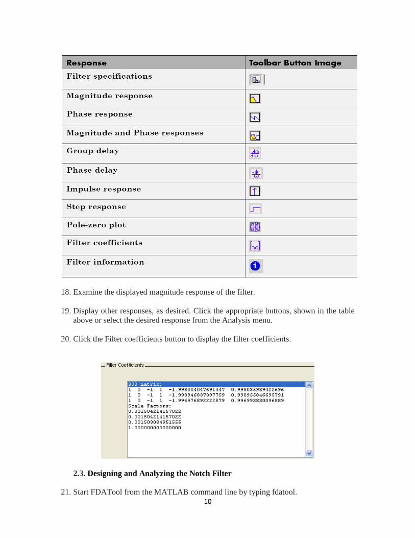
2.2. Analyzing the Octave-band Filter After designing the filter, you can view the following filter responses in the display region by clicking on the associated toolbar button or by selecting the desired response from the Analysis menu.

10

18. Examine the displayed magnitude response of the filter. 19. Display other responses, as desired. Click the appropriate buttons, shown in the table

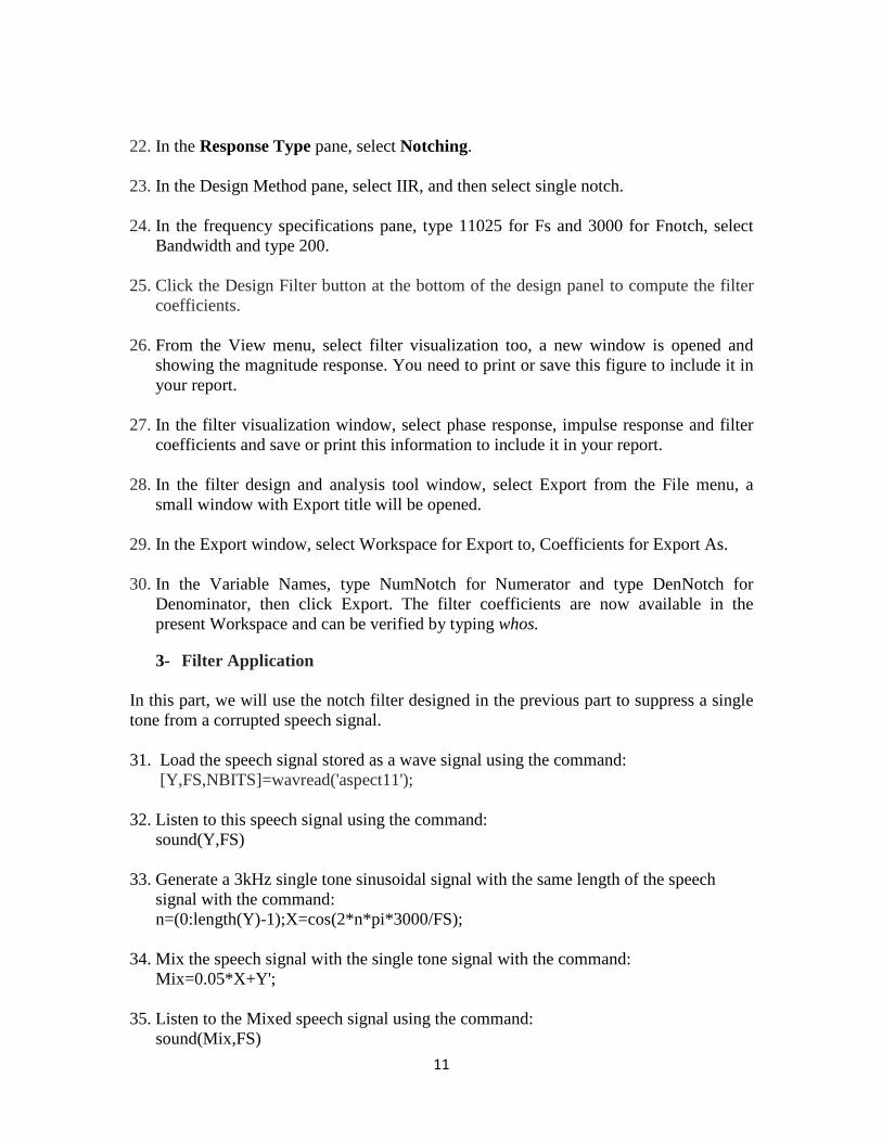
above or select the desired response from the Analysis menu. 20. Click the Filter coefficients button to display the filter coefficients.

2.3. Designing and Analyzing the Notch Filter 21. Start FDATool from the MATLAB command line by typing fdatool.

11

22. In the Response Type pane, select Notching. 23. In the Design Method pane, select IIR, and then select single notch. 24. In the frequency specifications pane, type 11025 for Fs and 3000 for Fnotch, select

Bandwidth and type 200. 25. Click the Design Filter button at the bottom of the design panel to compute the filter

coefficients. 26. From the View menu, select filter visualization too, a new window is opened and

showing the magnitude response. You need to print or save this figure to include it in your report.

27. In the filter visualization window, select phase response, impulse response and filter

coefficients and save or print this information to include it in your report. 28. In the filter design and analysis tool window, select Export from the File menu, a

small window with Export title will be opened. 29. In the Export window, select Workspace for Export to, Coefficients for Export As. 30. In the Variable Names, type NumNotch for Numerator and type DenNotch for

Denominator, then click Export. The filter coefficients are now available in the present Workspace and can be verified by typing whos.

3- Filter Application

In this part, we will use the notch filter designed in the previous part to suppress a single tone from a corrupted speech signal. 31. Load the speech signal stored as a wave signal using the command: [Y,FS,NBITS]=wavread('aspect11'); 32. Listen to this speech signal using the command:

sound(Y,FS)

33. Generate a 3kHz single tone sinusoidal signal with the same length of the speech signal with the command: n=(0:length(Y)-1);X=cos(2*n*pi*3000/FS);

34. Mix the speech signal with the single tone signal with the command: Mix=0.05*X+Y';

35. Listen to the Mixed speech signal using the command: sound(Mix,FS)

12

36. Evaluate and plot the amplitude spectrum of both the original speech signal and the

mixed signal with the command: HY= Single_Sided_Amplitude_Spectrum(Y,FS); HMix= Single_Sided_Amplitude_Spectrum(Mix,FS); Notice the presence of high spike at frequency 3kHz in the later spectrum.

37. To suppress the single tone from the corrupted speech signal use the notch filter

designed in the previous part. First, verify the response of the filter using the command: freqz(NumNotch,DenNotch) A figure of both the amplitude and phase response of the filter will be created. Then, use the following command to apply the notch filter to the mixed signal: YF=filter(NumNotch,DenNotch,Mix);

38. Verify the suppression of the single tone from the mixed signal by plotting and listening to the filtered signal YF using the Single_Sided_Amplitude_Spectrum and the sound functions

13

Experiment 2A Introduction to the Digital Signal Processing Kit (DSK) and

the Code Composer Studio (CCS) Objectives:

1- To become familiar with the DSK and its audio connections. 2- Test the operation of the DSK and CCS.

Lab Equipments: 1- DSK Board. 2- CCS software installed on the computer. 3- Oscilloscope. 4- Headphone.

Description:

1- The C6713 DSK Board The DSK packages are powerful, yet relatively inexpensive, with the necessary hardware and software support tools for real - time signal processing. They are complete DSP systems. A simplified block diagram of the DSK is shown in Figure 2A.1.

The major DSK hardware features are:

• A TMS320C6713 DSP operating at 225 MHz.

14

• 16 - bit stereo codec TLV320AIC23 (AIC23) for analog input and output. The onboard codec AIC23 uses sigma – delta technology that provides analog - to - digital conversion (ADC) and digital - to - analog conversion (DAC) functions. It uses a 12 - MHz system clock and its sampling rate can be selected from a range of alternative settings from 8 to 96 kHz.

• A daughter card expansion facility

• Two 80 - pin connectors provide for external peripheral and external memory interfaces.

• 16 MB (megabytes) of synchronous dynamic RAM (SDRAM).

• 512 Kbytes of Flash memory (256 Kbytes usable in default configuration).

• Four connectors on the boards provide analog input and output: MIC IN for microphone input, LINE IN for line input, LINE OUT for line output, and HEADPHONE for a headphone output (multiplexed with line output).

• Four user accessible LEDs and DIP switches.

• Voltage regulators that provide 1.26 V for the DSP cores and 3.3 V for their memory and peripherals.

2- Software Support for the DSK Board and ’C6x DSP’s 2.1 The Board Support Library (BSL)

A special Board Support Library (BSL) is supplied with the TMS320C6713 DSK. The BSL provides C-language functions for configuring and controlling all the on-board devices. The library includes modules for general board initialization, access to the AIC23 codec, reading the DIP switches, controlling the LED’s, and programming and erasing the Flash memory. The source code for this library is also included. The version of Code Composer supplied with the DSK is set up to automatically use the BSL. You can get complete documentation for the BSL by connecting the DSK to your PC, bring up Code Composer, and going to Help, Contents, TMS320C6713DSK, Software, Board Support Library. 2.2 The Chip Support Library (CSL) Chip Support Library contains C functions and macros for configuring and interfacing with all the ’C6713 on-chip peripherals and CPU interrupt controller. This library is loaded onto the PC when the DSK software is installed. The CSL header files provide a complete symbolic description of all peripheral registers and register fields.

3- Code Composer Studio (CCS) Code Composer Studio (CCS) provides an integrated development environment (IDE) for real - time digital signal processing applications based on the C programming language. It

15

incorporates a C compiler, an assembler, and a linker. It has graphical capabilities and supports real - time debugging. The C compiler compiles a C source program with extension .c to produce an assembly source file with extension .asm. The assembler assembles an .asm source file to produce a machine language object file with extension .obj. The linker combines object files and object libraries as input to produce an executable file with extension .out. This executable file represents a linked common object file format (COFF), popular in Unix - based systems and adopted by several makers of digital signal processors. This executable file can be loaded and run directly on the digital signal processor. A Code Composer Studio project comprises all of the files (or links to all of the files) required in order to generate an executable file. A variety of options enabling files of different types to be added to or removed from a project are provided. In addition, a Code Composer Studio project contains information about exactly how files are to be used in order to generate an executable file. Compiler/linker options can be specified. A number of debugging features are available, including setting breakpoints and watching variables, viewing memory, registers, and mixed C and assembly code, graphing results, and monitoring execution time. One can step through a program in different ways (step into, or over, or out). Real - time analysis can be performed using CCS’s real - time data exchange (RTDX) facility. This allows for data exchange between the host PC and the target DSK as well as analysis in real - time without halting the target. 3.1 Project Files and Building Programs You can build a project in CCS to easily manage an application involving multiple source files, libraries, memory maps, and special command files. The file containing all the project information is given the extension pjt. By clicking on the Rebuild All or Incremental build task bar buttons or by menu selections. 3.2 The Optimizing Compiler and Assembler Code Composer Studio includes a C/C++ optimizing compiler that converts standard ANSI C source programs into C6000 assembly language source. The compiler has several extensions to ANSI C. Assembly statements can be included inline with the C source code. This is useful for manipulating registers in the DSP and using special hardware features that are not efficiently accessible thorough C. TI has created a language called linear assembly that is part way between pure assembly language and C. Linear assembly source files have the extension sa. In linear assembly you do not have to be concerned with assigning registers. Symbolic names can be used for registers. The assembly optimizer assigns registers and optimizes loops to generate highly parallel assembly code. The assembly source code files generated by the compiler and optimizing assembler must then be passed through the assembler to generate relocatable object modules. 3.3 The Linker The final step in building a program is to link all the relocatable modules together. The linker, lnk6x.exe, combines relocatable object modules to form an executable output

16

program. The default extension for executable programs is out. In addition, the linker can generate a map file showing the absolute memory addresses of all global variables. A very important input to the linker is a linker command file which has the extension cmd. The command file can contain names of additional object modules to link, paths to libraries, names for the map and out files, a memory map for the target hardware system, and commands describing where to put specific program sections in memory.

4- File Types You will be working with a number of files with different extensions. They include: 1. file.pjt : to create and build a project named file. 2. file.c : C source program. 3. file.asm : assembly source program created by the user, by the C compiler,or by the

linear optimizer. 4. file.sa : linear assembly source program. The linear optimizer uses file.sa as input to

produce an assembly program file.asm . 5. file.h : header support file. 6. file.lib : library file, such as the run - time support library file rts6700.lib . 7. file.cmd : linker command file that maps sections to memory. 8. file.obj : object file created by the assembler. 9. file.out : executable file created by the linker to be loaded and run on the C6713

processor. 10. file.cdb : configuration file when using DSP/BIOS. LAB WORK:

1- QUICK TESTS OF THE DSK (ON POWER ON AND USING CCS) 1. Check out the hardware. Find the three audio connectors for the DSK. They are MIC

IN, LINE IN, and LINE OUT. The MIC IN jack is for low level signals from a microphone.

You will be using the commercial signal generator for this course and should use only the LINE IN and LINE OUT connectors for these larger signal levels. Beware that a common mistake of lab students is to make the input too large and saturate the input amplifiers resulting in strange outputs.

2. On power on, a power on self - test (POST) program, stored by default in the onboard flash memory, uses routines from the board support library (BSL) to test the DSK. It tests the internal, external, and flash memory, the two multichannel buffered serial ports (McBSP), DMA, the onboard codec, and the LEDs. If all tests are successful, all four LEDs blink three times and stop (with all LEDs on). During the testing of the codec, a 1 - kHz tone is generated for 1 second.

3. Launch CCS from the icon on the desktop. A USB enumeration process will take place and the Code Composer Studio window will open.

17

4. Click on Debug →Connect and you should see the message “The target is now connected” appear (for a few seconds) in the bottom left - hand corner of the CCS window.

5. Click on GEL →Check DSK →QuickTest . The Quick Test can be used for confirmation of correct operation and installation. A message of the following form should then be displayed in a new window within CCS:

Switches:15 Board Revision:2 CPLDRevision: 2

The value displayed following the label Switches reflects the state of the four DIP switches on the edge of the DSK circuit board. A value of 15 corresponds to all four switches in the up position. Change the switches to (1110) 2, that is, the first three switches (0, 1, 2) up and the fourth switch (3) down. Click again on GEL →Check DSK →QuickTest and verify that the value displayed is now 7 (“Switches: 7”). You can set the value represented by the four user switches from 0 to 15. Programs running on the DSK can test the state of the DIP switches and react accordingly. The values displayed following the labels Board Revision and CPLD Revision depend on the type and revision of the DSK circuit board. 6. Click on Debug → Disconnect

2- Alternative Quick Test of DSK

7. Open/launch CCS from the icon on the desktop if not done already.

8. Select Debug →Connect and check that the symbol in the bottom left – hand corner of the CCS window indicates connection to the DSK.

9. Select File →Load Program and load the file c: \ CCStudio_v3.1 \ MyProjects \sine8_LED \ Debug \ sine8_LED.out. This loads the executable file sine8_LED.out into the digital signal processor.

10.Select Debug →Run.

Check that the DSP is running. The word RUNNING should be displayed in the bottom left - hand corner of the CCS window. Press DIP switch #0 down. LED #0 should light and a 1 - kHz tone should be generated by the codec. Connect the LINE OUT (or the HEADPHONE) socket on the DSK board to a speaker, an oscilloscope, or headphones and verify the generation of the 1 - kHz tone. The four connectors on the DSK board for input and output (MIC, LINE IN, LINE OUT, and HEADPHONE) each use a 3.5 - mm jack audio cable. Halt execution of program sine8_LED.out by selecting Debug →Halt. 11.Select Debug →Disconnect.

12.Close the CCS program.

18

Experiment 2B Sine Wave Generation Using Eight points with DIP Switch Control

Objectives:

1- To generate a sinusoidal analog output waveform using a table-lookup method.

2- To illustrate some of the features of the CCS for editing source files, building a project, accessing the code generation tools, and running a program on the C6713 processor.

Lab Equipments:

1- DSK Board. 2- CCS software installed on the computer. 3- Oscilloscope. 4- Headphone.

Description: The C source file sine8_LED.c listed in Figure 2B.1 is included in the folder sine8_LED .

19

The operation of program sine8_LED.c is as follows. An array, sine_table, of eight 16 - bit signed integers is declared and initialized to contain eight samples of exactly one cycle of a sinusoid. The value of sine_table[i] is equal to

Within function main(), calls to functions comm_poll(), DSK6713_LED_init() ,and DSK6713_DIP_init() initialize the DSK, the AIC23 codec onboard the DSK, and the two multichannel buffered serial ports (McBSPs) on the C6713 processor. Function comm_poll() is defined in the file c6713dskinit.c , and functions DSK6713_LED_init() and DSK6713_DIP_init() are supplied in the board support library (BSL) file dsk6713bsl.lib . The program statement while (1) within the function main() creates an infinite loop. Within that loop, the state of DIP switch #0 is tested and if it is pressed down, LED #0 is switched on and a sample from the lookup table is output. If DIP switch #0 is not pressed down then LED #0 is switched off. As long as DIP switch #0 is pressed down, sample values read from the array sine_table will be output and a sinusoidal analog output waveform will be generated via the left - hand channel of the AIC23 codec and the LINE OUT and HEADPHONE sockets. Each time a sample value is read from the array sine_table , multiplied by the value of the variable gain , and written to the codec, the index, loopindex , into the array is incremented and when its value exceeds the allowable range for the array ( LOOPLENGTH - 1 ), it is reset to zero. Each time the function output_left_sample() , defined in source file C6713dskinit.c , is called to output a sample value, it waits until the codec, initialized by the function comm_poll() to output samples at a rate of 8 kHz, is ready for the next sample. In this way, once DIP switch #0 has been pressed down it will be tested at a rate of 8 kHz. The sampling rate at which the codec operates is set by the program statement Uint32 fs = DSK6713_AIC23_FREQ_8KHZ; One cycle of the sinusoidal analog output waveform corresponds to eight output samples and hence the frequency of the sinusoidal analog output waveform is equal to the codec sampling rate (8 kHz) divided by eight, that is, 1 kHz. LAB WORK:

1- Creating a Project

This experiment illustrates how to create a project, adding the necessary files to generate an executable file sine8_LED.out. a file named sine8_LED.pjt is already exist at c:\CCStudio_v3.1\MyProjects\sine8_LED. However, for the purposes of gaining familiarity with CCS, this experiment will illustrate how to create that project file from scratch. 1. Delete the existing project file sine8_LED.pjt in folder

c:\CCStudio_v3.1\myprojects\sine8_LED. Do this from outside CCS. 2. Launch CCS by double - clicking on its desktop icon.

20

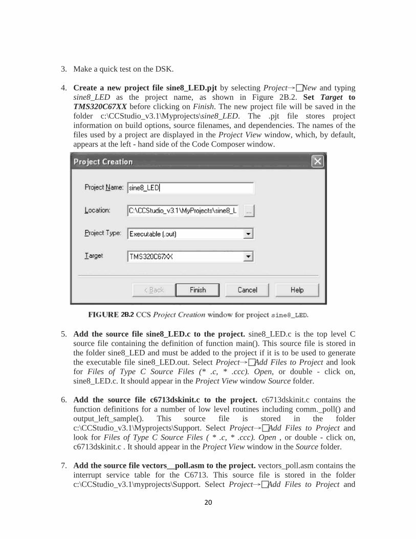
3. Make a quick test on the DSK. 4. Create a new project file sine8_LED.pjt by selecting Project→New and typing

sine8_LED as the project name, as shown in Figure 2B.2. Set Target to TMS320C67XX before clicking on Finish. The new project file will be saved in the folder c:\CCStudio_v3.1\Myprojects\sine8_LED. The .pjt file stores project information on build options, source filenames, and dependencies. The names of the files used by a project are displayed in the Project View window, which, by default, appears at the left - hand side of the Code Composer window.

5. Add the source file sine8_LED.c to the project. sine8_LED.c is the top level C

source file containing the definition of function main(). This source file is stored in the folder sine8_LED and must be added to the project if it is to be used to generate the executable file sine8_LED.out. Select Project→Add Files to Project and look for Files of Type C Source Files (* .c, * .ccc). Open, or double - click on, sine8_LED.c. It should appear in the Project View window Source folder.

6. Add the source file c6713dskinit.c to the project. c6713dskinit.c contains the

function definitions for a number of low level routines including comm._poll() and output_left_sample(). This source file is stored in the folder c:\CCStudio_v3.1\Myprojects\Support. Select Project→Add Files to Project and look for Files of Type C Source Files ( * .c, * .ccc). Open , or double - click on, c6713dskinit.c . It should appear in the Project View window in the Source folder.

7. Add the source file vectors__poll.asm to the project. vectors_poll.asm contains the

interrupt service table for the C6713. This source file is stored in the folder c:\CCStudio_v3.1\myprojects\Support. Select Project→Add Files to Project and

21

look for Files of Type ASM Source Files (* .a *). Open, or double - click on, vectors_poll.asm. It should appear in the Project View window in the Source folder.

8. Add library support files rts6700.lib, dsk6713bsl.lib, and csl6713.lib to the

project. Three more times, select Project→Add Files to Project and look for Files of Type Object and Library Files (* .o * , * .l * ) The three library files are stored in folders c:\CCStudio_v3.1\c6000\cgtools\lib, c:\ CCStudio_v3.1\c6000\dsk6713\lib, and c:\CCStudio_v3.1\c6000\csl\lib, respectively. These are the run - time support (for C67x architecture), board support (for C6713 DSK), and chip support (for C6713 processor) library files.

9. Add the linker command file c6713dsk.cmd to the project. This file is stored in the

folder c:\CCStudio_v3.1\myprojects\Support. Select Project→Add Files to Project and look for Files of Type Linker Command File (* .cmd; * .lcf) . Open, or double - click on, c6713dsk.cmd. It should then appear in the Project View window.

10. No header files will be shown in the Project View window at this stage. Selecting

Project→Scan All File Dependencies will rectify this. You should now be able to see header files c6713dskinit.h, dsk6713.h, and dsk6713_aic23.h , in the Project View window.

11. The Project View window in CCS should look as shown in Figure 2B.3. The GEL

file dsk6713.gel is added automatically when you create the project. It initializes the C6713 DSK invoking the board support library to use the PLL to set the CPU clock to 225 MHz (otherwise the C6713 runs at 50 MHz by default). Any of the files (except the library files) listed in the Project View window can be displayed (and edited) by double - clicking on their name in the Project View window. You should not add header or include files to the project. They are added to the project automatically when you select Scan All File Dependencies . (They are also added when you build the project.) Verify from the Project View window that the project ( .pjt ) file, the linker command ( .cmd ) file, the three library ( .lib ) files, the two C source ( .c ) files, and the assembly ( .asm ) file have been added to the project.

22

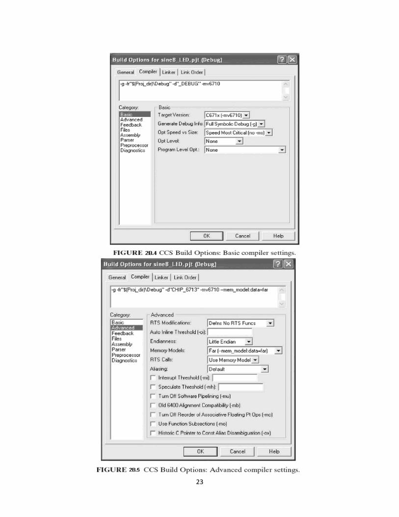
2- Code Generation and Build Options The code generation tools underlying CCS, that is, C compiler, assembler, and linker, have a number of options associated with each of them. These options must be set appropriately before attempting to build a project. Once set, these options will be stored in the project file. 2.1. Setting Compiler Options Select Project→Build Options and click on the Compiler tab. Set the following options, as shown in Figures 2B.4, 2B.5, and 2B.6.In the Basic category set Target Versionto C671x (- mv6710). In the Advanced category set Memory Models to Far ( – mem_ model:data=far) . In the Preprocessor category set Pre - Defi ne Symbol to CHIP_6713 and Include Search Path to c:\ CCStudio_v3.1 \ C6000 \ dsk6713 \ include. Click on OK.

23

24

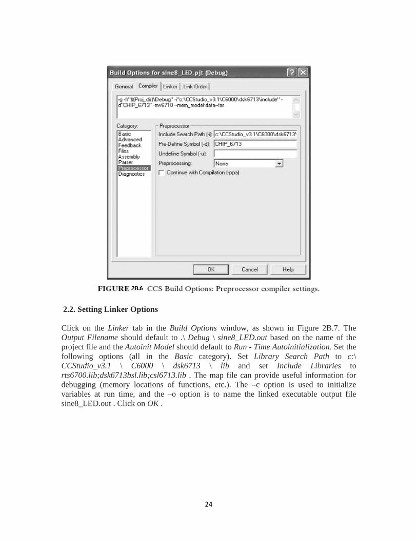
2.2. Setting Linker Options Click on the Linker tab in the Build Options window, as shown in Figure 2B.7. The Output Filename should default to .\ Debug \ sine8_LED.out based on the name of the project file and the Autoinit Model should default to Run - Time Autoinitialization. Set the following options (all in the Basic category). Set Library Search Path to c:\ CCStudio_v3.1 \ C6000 \ dsk6713 \ lib and set Include Libraries to rts6700.lib;dsk6713bsl.lib;csl6713.lib . The map file can provide useful information for debugging (memory locations of functions, etc.). The –c option is used to initialize variables at run time, and the –o option is to name the linked executable output file sine8_LED.out . Click on OK .

25

3- Building , Downloading and Running the Project

The project sine8_LED can now be built, and the executable file sine8_LED.out can be downloaded to the DSK and run.

12. Build this project as sine8_LED. Select Project→Rebuild All. Or press the toolbar

button with the three downward arrows. This compiles and assembles all the C files using cl6x and assembles the assembly file vectors_poll.asm using asm6x. The resulting object files are then linked with the library files using lnk6x . This creates an executable file sine8_LED.out that can be loaded into the C6713 processor and run. Note that the commands for compiling, assembling, and linking are performed with the Build option. A log file cc_build_Debug.log is created that shows the files that are compiled and assembled, along with the compiler options selected. It also lists the support functions that are used. The building process causes all the dependent files to be included (in case one forgets to scan for all the file dependencies). You should see

26

a number of diagnostic messages, culminating in the message “ Build Complete, 0 Errors, 0 Warnings, 0 Remarks ” appear in an output window in the bottom left - hand side of the CCS window. It is possible that a warning about the Stack Size will have appeared. This can be ignored or can be suppressed by unchecking the Warn About Output Sections option in the Advanced category of Linker Build Options. Alternatively, it can be eliminated by setting the Stack Size option in the Advanced category of Linker Build Options to a suitable value (e.g., 0x1000 ). Connect to the DSK . Select Debug→Connect and check that the symbol in the bottom left - hand corner of the CCS window indicates connection to the DSK.

13. Select File→Load Program in order to load sine8_LED.out. It should be stored in the folder c:\CCStudio_v3.1\MyProjects\sine8_LED\Debug. Select Debug→Run. In order to verify that a sinusoidal output waveform with a frequency of 1 kHz is present at both the LINE OUT and HEADPHONE sockets on the DSK, when DIP switch #0 is pressed down, use an oscilloscope connected to the LINE OUT socket and a pair of headphones connected to the HEADPHONE socket.

4- Monitoring the Watch Window

Ensure that the processor is still running (and that DIP switch #0 is pressed down). Note the message “RUNNING” displayed at the bottom left of CCS. The Watch window allows you to change the value of a parameter or to monitor a variable: 14. Select View →Quick Watch. Type gain, and then click on Add to Watch. The gain

value of 10 set in the program in Figure 2B.1 should appear in the Watch window. 15. Change gain from 10 to 30 in the Watch window. Press enter. Verify that the

amplitude of the generated tone has increased (with the processor still running and DIP switch #0 pressed down). The amplitude of the sine wave should have increased from approximately 0.9 V p - p to approximately 2.5 V p - p.

5- Using a GEL Slider to Control the Gain

The General Extension Language (GEL) is an interpreted language similar to (a subset of) C. It allows you to change the value of a variable (e.g., gain) while the processor is running. 16. Select File →Load GEL and load the file gain.gel (in folder sine8_LED ). 17. Double - click on the filename gain.gel in the Project View window to view it within

CCS. The file is listed in Figure 2B.8. The format of a slider GEL function is

27

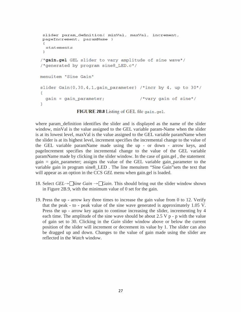
where param_definition identifies the slider and is displayed as the name of the slider window, minVal is the value assigned to the GEL variable param-Name when the slider is at its lowest level, maxVal is the value assigned to the GEL variable paramName when the slider is at its highest level, increment specifies the incremental change to the value of the GEL variable paramName made using the up - or down - arrow keys, and pageIncrement specifies the incremental change to the value of the GEL variable paramName made by clicking in the slider window. In the case of gain.gel , the statement gain = gain_parameter; assigns the value of the GEL variable gain_parameter to the variable gain in program sine8_LED . The line menuitem “Sine Gain”sets the text that will appear as an option in the CCS GEL menu when gain.gel is loaded. 18. Select GEL→Sine Gain →Gain. This should bring out the slider window shown

in Figure 2B.9, with the minimum value of 0 set for the gain. 19. Press the up - arrow key three times to increase the gain value from 0 to 12. Verify

that the peak - to - peak value of the sine wave generated is approximately 1.05 V. Press the up - arrow key again to continue increasing the slider, incrementing by 4 each time. The amplitude of the sine wave should be about 2.5 V p - p with the value of gain set to 30. Clicking in the Gain slider window above or below the current position of the slider will increment or decrement its value by 1. The slider can also be dragged up and down. Changes to the value of gain made using the slider are reflected in the Watch window.

28

6- Changing the Frequency of the Generated Sinusoid There are several different ways in which the frequency of the sinusoid generated by program sine8_LED.c can be altered. 20. Change the AIC23 codec sampling frequency from 8 kHz to 16 kHz by changing the

line that reads Uint32 fs = DSK6713_AIC23_FREQ_8KHZ; to read Uint32 fs = DSK6713_AIC23_FREQ_16KHZ; Rebuild (use incremental build) the project, load and run the new executable file, and verify that the frequency of the generated sinusoid is 2 kHz. The sampling frequencies supported by the AIC23 codec are 8, 16, 24, 32, 44.1, 48, and 96 kHz.

21. Change the number of samples stored in the lookup table to four. By changing the

lines that read #define LOOPLENGTH 8 short sine_table[LOOPLENGTH]={0,707,1000,707,0, -707,0,-1000,-707}; to read #define LOOPLENGTH 4 short sine_table[LOOPLENGTH]={0,1000,0, -1000}; Verify that the frequency of the sinusoid generated is 2 kHz (assuming an 8 - kHz sampling frequency).

Remember that the sinusoid is no longer generated if the DIP switch #0 is not pressed down. A different DIP switch can be used to control whether or not a sinusoid is generated by changing the value of the parameter passed to the functions DSK6713_DIP_get(), DSK6713_LED_on(), and DSK6713_LED_off() . Suitable values are 0, 1, 2, and 3.

29

Two sliders can readily be used, one to change the gain and the other to change the frequency. A different signal frequency can be generated, by changing the incremental changes applied to the value of loopindex within the C program (e.g., stepping through every two points in the table). When you exit CCS after you build a project, all changes made to the project can be saved. You can later return to the project with the status as you left it before. For example, when returning to the project, after launching CCS, select Project→Open to open an existing project such as sine8_LED.pjt (with all the necessary files for the project already added).

30

Experiment 2C Generation of sinusoid and Plotting with CCS (sine8_buf)

Objectives:

1- To generate a sinusoidal analog output waveform using eight pre-calculated and pre-stored sample values.

2- To illustrate the capabilities of CCS for plotting data in both time and frequency domains.

Lab Equipments:

1- DSK Board. 2- CCS software installed on the computer. 3- Oscilloscope. 4- Headphone.

Description: This example generates a sinusoidal analog output signal using eight pre[calculated and pre[stored sample values. However, it differs fundamentally from sine8_LED in that its operation is based on the use of interrupts. In addition, it uses a buffer to store the BUFFERLENGTH most recent output samples. It is used to illustrate the capabilities of CCS for plotting data in both time and frequency domains. All the files necessary to build and run an executable file sine8_BUF.out are stored in folder sine8_buf. Program file sine8_buf.c is listed in Figure 2C.1. This program uses interrupt- driven input/output rather than polling, so that the file vectors_intr.asm is used in place of vectors_poll.asm. The interrupt service table specified in vectors_intr.asm associates the interrupt service routine c_int11() with hardware interrupt INT11, which is asserted by the AIC23 codec on the DSK at each sampling instant. Within function main() , function comm_intr() is used in place of comm_poll() . This function is defined in file c6713dskinit.c. Essentially, it initializes the DSK hardware, including the AIC23 codec, such that the codec sampling rate is set according to the value of the variable fs and the codec interrupts the processor at every sampling instant. The statement while(1) in function main() creates an infinite loop, during which the processor waits for interrupts. On interrupt, execution proceeds to the interrupt service routine (ISR) c_int11() , which reads a new sample value from the array sine_table and writes it both to the array out_buffer and to the DAC using function output_left_sample(). Because a project file sine8_buf.pjt is supplied, there is no need to create a new project file, add files to it, or alter compiler and linker build options. In order to build, download and run program sine8_buf.c.

31

LAB WORK: 1. Launch CCS by double - clicking on its desktop icon. 2. Make a quick test on the DSK. 3. Open project sine8_buf.pjt by selecting Project →Open and double – clicking on

file sine8_buf.pjt in folder sine8_buf. 4. Build this project as sine8_buf. Load and run the executable file sine8_buf.out and

verify that a 1 - kHz sinusoid is generated at the LINE OUT and HEADPHONE sockets

Graphical Displays in CCS The array out_buffer is used to store the BUFFERLENGTH most recently output sample values. Once program execution has been halted, the data stored in out_buffer can be displayed graphically in CCS.

32

5. Select View→Graph →Time/Frequency and set the Graph Property Dialog properties as shown in Figure 2C.2.a. Figure 2C.2.b. shows the resultant Graphical Display window.

6. Figure 2C.3.a shows the Graph Property Dialog window that corresponds to the

frequency domain representation of the contents of out_buffer shown in Figure 2C.3.b. The spike at 1 kHz represents the frequency of the sinusoid generated by program sine8_buf.c .

33

Viewing and Saving Data from Memory into File 7. To view the contents of out_buffer, select View→Memory. Specify out_buffer as

the Address and select 32 - bit Signed Integer as the Format , as shown in Figure 2C.4.a. The resultant Memory window is shown in Figure 2C.4.b.

8. To save the contents of out_buffer to a file, select File→Data →Save. Save the

file as sine8_buf.dat , selecting data type Integer , in the folder sine8_buf. In the Storing Memory into File window, specify out_buffer as the Address and a Length of 256. The resulting file is a text file and you can plot this data using other applications (e.g., MATLAB).

34

Although the values stored in array sine_table and passed to function output_left_sample() are 16 - bit signed integers, array out_buffer is declared as type int (32 - bit signed integer) in program sine8_buf.c to allow for the fact that there is no 16 - bit Signed Integer data type option in the Save Data facility in CCS.

35

Experiment 3A Basic Input and Output Using Polling (loop_poll)

Objectives:

1- Sampling and reconstruction of real time signals. 2- Gain change of the line input.

Lab Equipments: 1- DSK Board. 2- CCS software installed on the computer. 3- Oscilloscope. 4- Headphone. 5- Signal Generator.

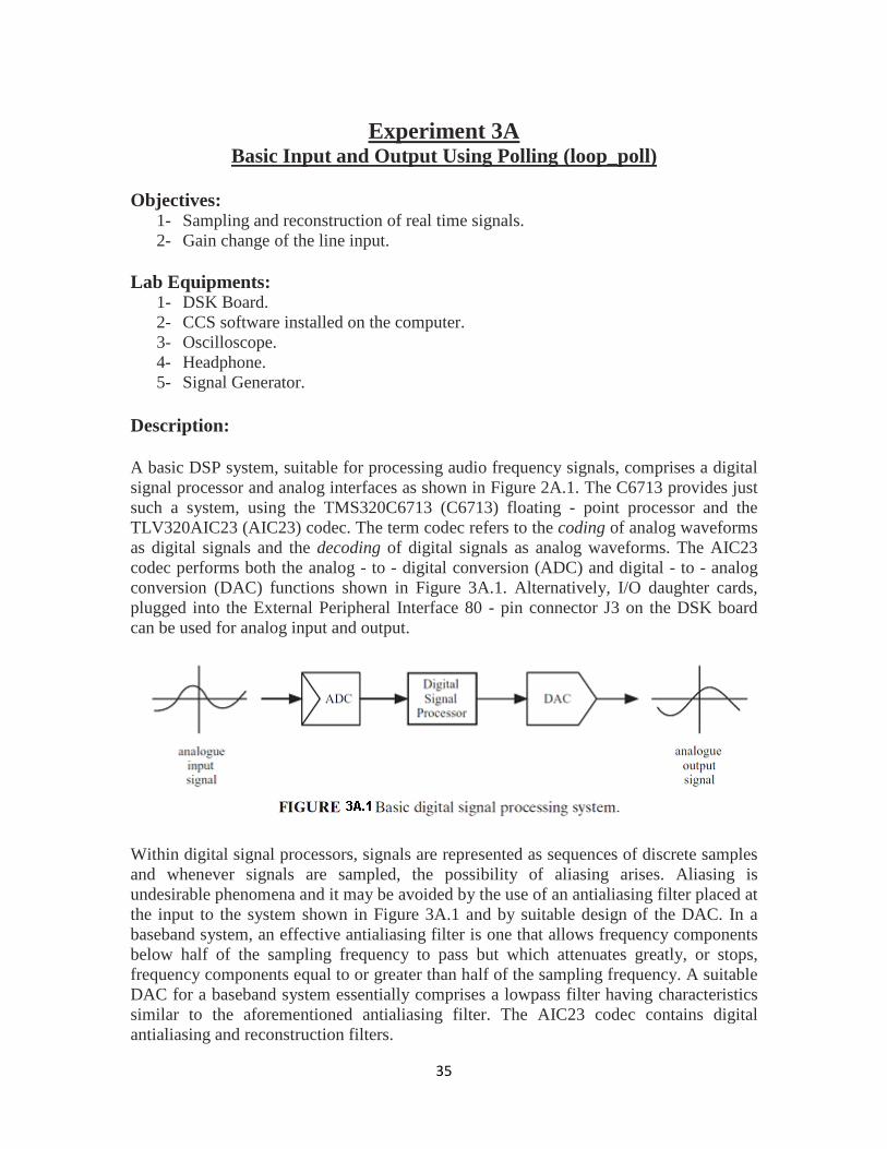
Description: A basic DSP system, suitable for processing audio frequency signals, comprises a digital signal processor and analog interfaces as shown in Figure 2A.1. The C6713 provides just such a system, using the TMS320C6713 (C6713) floating - point processor and the TLV320AIC23 (AIC23) codec. The term codec refers to the coding of analog waveforms as digital signals and the decoding of digital signals as analog waveforms. The AIC23 codec performs both the analog - to - digital conversion (ADC) and digital - to - analog conversion (DAC) functions shown in Figure 3A.1. Alternatively, I/O daughter cards, plugged into the External Peripheral Interface 80 - pin connector J3 on the DSK board can be used for analog input and output.

Within digital signal processors, signals are represented as sequences of discrete samples and whenever signals are sampled, the possibility of aliasing arises. Aliasing is undesirable phenomena and it may be avoided by the use of an antialiasing filter placed at the input to the system shown in Figure 3A.1 and by suitable design of the DAC. In a baseband system, an effective antialiasing filter is one that allows frequency components below half of the sampling frequency to pass but which attenuates greatly, or stops, frequency components equal to or greater than half of the sampling frequency. A suitable DAC for a baseband system essentially comprises a lowpass filter having characteristics similar to the aforementioned antialiasing filter. The AIC23 codec contains digital antialiasing and reconstruction filters.

36

The C6713 DSK makes use of the TLV320AIC23 (AIC23) codec for analog input and output. The analog - to - digital converter (ADC), or coder, part of the codec converts an analog input signal into a sequence of sample values (16 – bit signed integer) to be processed by the digital signal processor. The digital - to – analog converter (DAC), or decoder, part of the codec reconstructs an analog output signal from a sequence of sample values (16 - bit signed integer) that have been processed by the digital signal processor. The AIC23 is a stereo audio codec based on sigma – delta technology. A 12 - MHz crystal supplies the clock to the AIC23 codec (also to the DSP and the USB interface). Using this 12 - MHz master clock, with oversampling rates of 250Fs and 272Fs , exact audio sample rates of 48 kHz (12 MHz/250) and the CD rate of 44.1 kHz (12 MHz/272) can be obtained. The sampling rate of the AIC23 can be configured to be 8, 16, 24, 32, 44.1, 48, or 96 kHz. Communication with the AIC23 codec for input and output uses two multichannel buffered serial ports (McBSPs) on the C6713. McBSP0 is used as a unidirectional channel to send a 16 - bit control word to the AIC23. McBSP1 is used as a bidirectional channel to send and receive audio data. The codec can be configured for data - transfer word-lengths of 16, 20, 24, or 32 bits. The LINE IN and HEADPHONE OUT signal paths within the codec contain configurable gain elements with ranges of 12 to − 34 dB in steps of 1.5 dB, and 6 to − 73 dB in steps of 1 dB, respectively. Most of the programming examples in this booklet configure the codec for a sampling rate of 8 kHz, 32 - bit data transfer, and 0 - dB gain in the LINE IN and HEADPHONE OUT signal paths. The maximum allowable input signal level at the LINE IN inputs to the codec is 1 V rms. However, the C6713 DSK contain a potential divider circuit with a gain of 0.5 between their LINE IN sockets and the codec itself with the effect that the maximum allowable input signal level at the LINE IN sockets on the DSK is 2 V rms. Above this level, input signals will be distorted. Input and output sockets on the DSK are ac coupled to the codec. The C language source file for a program, loop_poll.c , that simply copies input samples read from the AIC23 codec ADC back to the AIC23 codec DAC as output samples is listed in Figure3A.2. Effectively, the MIC input socket is connected straight through to the HEADPHONE OUT socket on the DSK via the AIC23 codec and the digital signal processor. loop_poll.c uses the same polling technique for real - time input and output as program sine8_LED.c , presented in previous experiment .

37

Input and Output Functions Defined in Support File c6713dskinit.c The functions input_left_sample() , output_left_sample() , and comm_poll() are defined in the support file c6713dskinit.c. This way the C source file loop_poll.c is kept as small as possible and potentially distracting low level detail is hidden. The implementation details of these, and other, functions defined in c6713dskinit.c need not be studied in detail in order to carry out the examples presented in this booklet but are described here for completeness. Further calls are made by input_left_sample() and output_left_sample() to lower level functions contained in the board support library DSK6713bsl.lib. Function comm_poll() initializes the DSK and, in particular, the AIC23 codec such that its sample rate is set according to the value of the variable fs (assigned in loop_poll.c ), its input source according to the value of the variable inputsource (assigned in loop_poll.c), and polling mode is selected. Other AIC23 configuration settings are determined by the parameters specified in file c6713dskinit.h. These parameters include the gain settings in the LINE IN and HEADPHONE out signal paths, the digital audio interface format, and so on. Similar values for all of these parameters are used by almost all of the program examples in this booklet. Only rarely will they be changed and so it is convenient to hide them out of the way in file c6713dskinit.h . The two settings, sampling rate and input source, are changed sufficiently frequently, from one program example to another, that their values are set in each example program by initializing the values of the variables fs and inputsource. In function dsk6713_init() in file c6713dskinit.c , these values are used by functions DSK6713_AIC23_setFreq() and DSK6713_AIC23_rset(), respectively. In polling mode, function input_left_sample()

38

polls, or tests, the receive ready bit ( RRDY ) of the McBSP serial port control register ( SPCR ) until this indicates that newly converted data is available to be read using function MCBSP_read(). Function output_left_sample() polls, or tests, the transmit ready bit ( XRDY ) of the McBSP serial port control register ( SPCR ) until this indicates that the codec is ready to receive a new output sample. A new output sample is sent to the codec using function McBSP_write() . Although polling is simpler than the interrupt technique used in sine8_buf.c, it is less efficient since the processor spends nearly all of its time repeatedly testing whether the codec is ready either to transmit or to receive data. LAB WORK: 1. Launch CCS by double - clicking on its desktop icon. 2. Make a quick test on the DSK. 3. Open project loop_poll.pjt by selecting Project →Open and double – clicking on

file loop_poll.pjt in folder loop_poll. 4. Load and run the executable file loop_poll.out. 5. Use a microphone and headphones to verify that the program operates as intended. 6. Rebuild the program having changed the line that reads

Uint16 inputsource=DSK6713_AIC23_INPUT_MIC; to read Uint16 inputsource=DSK6713_AIC23_INPUT_LINE; in order to select the LINE IN rather than the MIC socket on the DSK.

7. Input a sinusoidal waveform to the LINE IN connector on the DSK, with amplitude of

approximately 2.0 V p - p and a frequency of approximately 1 kHz. 8. Connect the output of the DSK, LINE OUT, to an oscilloscope, and verify the

presence of a tone of the same frequency, but attenuated to approximately 1.0 V p - p. 9. Explain the attenuation occurred. 10. Increase the amplitude of the input sinusoidal waveform (at the LINE IN socket)

beyond 5V p – p. and verify that the output signal becomes distorted. Why? Changing the LINE IN Gain of the AIC23 Codec The AIC23 codec allows for the gain on left - and right - hand line - in input channels to be adjusted independently in steps of 1.5 dB by writing different values to the left and

39

right line input channel volume control registers. The values assigned to these registers by function comm_poll() are defined in the header file c6713dskinit.h . In order to change the values written, that file must be modified. 11. Copy the files c6713dskinit.h and C6713dskinit.c from the Support folder into the

folder loop_poll so that you don’t modify the original header file. 12. Remove these two files from the loop_poll project by right - clicking on

c6713dskinit.c in the Project View window and then selecting Project→ Remove from Project.

13. Add the copy of the file c6713dskinit.c in folder loop_poll to the project by selecting

Project → Add Files to Project. 14. Check that you have added the copy of file c6713dskinit.c to the project by right -

clicking on it in the Project View window and selecting Properties. 15. Select Project→ Scan all Dependencies in order to replace the file c6713dskinit.h

with the copy in folder loop_poll . 16. Edit the copy of file c6713dskinit.h included in the project (and stored in folder

loop_poll ), changing the line that reads 0x0017 / * Set -Up Reg 0 Left line volume control */ to read 0x001B / * Set -Up Reg 0 Left line volume control */

This modifies the value written to the AIC23 left line input channel gain register from 0x0017 to 0x001B and this increases the gain from 0 dB to 6 dB.

17. Build the project, making sure that the copy of the file c6713dskinit.c used in the

project is the copy in folder loop_poll. The header file c6713dskinit.h that will be included will come from that same folder

18. Load and run the executable file loop_poll.out and verify that the output signal is not

attenuated, but has the same amplitude as the input signal, that is, 2 V p - p.

40

Experiment 3B Basic Input and Output Using Interrupts (loop_intr)

Objectives:

1- Sampling and reconstruction of real time signals using the interrupt driven model.

2- Demonstration of echo and delay effects. Lab Equipments:

1- DSK Board. 2- CCS software installed on the computer. 3- Oscilloscope. 4- Headphone. 5- Signal Generator.

Description: Program loop_intr.c is functionally equivalent to program loop_poll.c but makes use of interrupts. This simple program is important because many of the other example programs in this booklet are based on the same interrupt - driven model. Instead of simply copying the sequence of samples representing an input signal to the codec output, a digital filtering operation can be performed each time a new input sample is received. It is worth taking time to ensure that you understand how program loop_intr.c works. In function main() , the initialization function comm_intr() is called. comm_intr() is very similar to comm_poll() but in addition to initializing the DSK, codec, and McBSP, and not selecting polling mode, it sets up interrupts such that the AIC23 codec will sample the analog input signal and interrupt the C6713 processor, at the sampling frequency defined by the line Uint32 fs=DSK6713_AIC23_FREQ_8KHZ; //set sampling rate It also initiates communication with the codec via the McBSP. In this example, a sampling rate of 8 kHz is used and interrupts will occur every 0.125 ms. (Sampling rates of 16, 24, 32, 44.1, 48, and 96 kHz are also possible.) Following initialization, function main() enters an endless while loop, doing nothing but waiting for interrupts. The functions that will act as interrupt service routines for the various different interrupts are specified in the interrupt service table contained in file vectors_intr.asm. This assembly language file differs from the file vectors_poll.asm in that function c_int11() is specified as the interrupt service routine for interrupt INT11. On interrupt, the interrupt service routine (ISR) c_int11() is called and it is within that routine that the most important program statements are executed. Function output_left_sample() is used to output a value read from the codec using function input_left_sample() .

41

Format of Data Transferred to and from AIC 23 Codec The AIC23 ADC converts left - and right - hand channel analog input signals into 16 - bit signed integers and the DAC converts 16 - bit signed integers to left - and right - hand channel analog output signals. Left - and right - hand channel samples are combined to form 32 - bit values that are communicated via the multichannel buffered serial port (McBSP) to and from the C6713. Access to the ADC and DAC from a C program is via the functions Uint32 input_sample(), short input_left_sample(), short input_right_sample(), void output_sample(int out_data) , void output_left_sample(short out_data), and void output_right_sample(short out_data). The 32 - bit unsigned integers (Uint32) returned by input_sample() and passed to output_sample() contain both left and right channel samples. The statement

In file dsk6713init.h declares a variable that may be handled either as one 32 - bit unsigned integer (AIC_data.uint) containing left and right channel sample values, or as two 16 - bit signed integers (AIC_data.channel[0] and AIC_data.channel[1] ). Most of the program examples in this booklet use only one channel for input and output and for clarity most use the functions input_left_sample() and output_left_sample() . These functions are defined in the file c6713dskinit.c, where the unpacking and packing

42

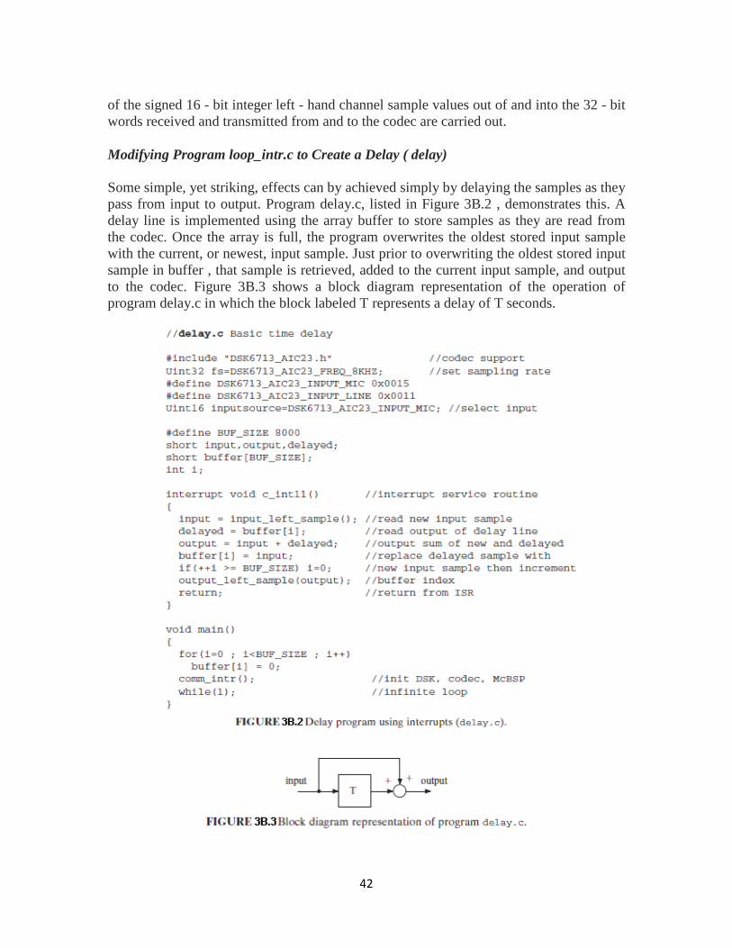
of the signed 16 - bit integer left - hand channel sample values out of and into the 32 - bit words received and transmitted from and to the codec are carried out. Modifying Program loop_intr.c to Create a Delay ( delay) Some simple, yet striking, effects can by achieved simply by delaying the samples as they pass from input to output. Program delay.c, listed in Figure 3B.2 , demonstrates this. A delay line is implemented using the array buffer to store samples as they are read from the codec. Once the array is full, the program overwrites the oldest stored input sample with the current, or newest, input sample. Just prior to overwriting the oldest stored input sample in buffer , that sample is retrieved, added to the current input sample, and output to the codec. Figure 3B.3 shows a block diagram representation of the operation of program delay.c in which the block labeled T represents a delay of T seconds.

43

Modifying Program loop_intr.c to Create an Echo ( echo) By feeding back a fraction of the output of the delay line to its input, a fading echo effect can be realized. Program echo.c, listed in Figure 3B.4, does this. Figure 3B.5 shows a block diagram representation of the operation of program echo.c. The value of the constant BUF_SIZE determines the number of samples stored in the array buffer and hence the duration of the delay. The value of the constant GAIN determines the fraction of the output that is fed back into the delay line and hence the rate at which the echo effect fades away. Setting the value of GAIN equal to or greater than unity would cause instability of the loop.

44

Build and run this project as echo. Experiment with different values of GAIN (between 0.0 and 1.0) and BUF_SIZE (between 100 and 8000). Source file echo.c must be edited and the project rebuilt in order to make these changes. Loop Program with Input Data Stored in a Buffer ( loop_buf ) Program loop_buf.c , listed in Figure 3B.6 , is an interrupt - based program and is stored in folder loop_buf . It is similar to program loop_intr.c except that it maintains a circular buffer in array buffer containing the BUF_SIZE most recent input sample values. Consequently, it is possible to display this data in CCS after halting the program.

45

LAB WORK: 1. Launch CCS by double - clicking on its desktop icon. 2. Make a quick test on the DSK. 3. Open project loop_intr.pjt by selecting Project →Open and double – clicking on

file loop_intr.pjt in folder loop_intr. 4. Load and run the executable file loop_intr.out. 5. Use a microphone and headphones to verify that the program operates as intended. 6. Halt the executable file loop_intr.out. 7. Open project delay.pjt by selecting Project →Open and double – clicking on file

delay.pjt in folder delay. 8. Load and run the executable file delay.out. 9. Use a microphone and headphones to verify that the program operates as intended. 10. Halt the executable file delay.out. 11. Open project echo.pjt by selecting Project →Open and double – clicking on file

echo.pjt in folder delay. 12. Load and run the executable file echo.out. 13. Experiment with different values of GAIN (between 0.0 and 1.0) and BUF_SIZE

(between 100 and 8000). Source file echo.c must be edited and the project rebuilt in order to make these changes.

14. Halt the executable file echo.out. 15. Use a signal generator connected to the LINE IN socket to input a sinusoidal signal

with a frequency between 100 and 3500 Hz. 16. Open project loop_buf.pjt by selecting Project →Open and double – clicking on file

loop_buf.pjt in folder loop_buf. 17. Load and run the executable file loop_buf.out. 18. Halt the program after a short time. 19. Select View → Graph → Time/Frequency in order to display the contents of array buffer.

46

Experiment 3C Sine Wave Generation Using sin() Function,

Reconstruction, Aliasing, and the Properties of the AIC 23 Codec

Objectives:

1- To generate sinusoidal signal using mathematical function. 2- Demonstration of aliasing in real time system. 3- To visualize the step response of the AIC23 Codec Anti-aliasing

Filter

Lab Equipments: 1- DSK Board. 2- CCS software installed on the computer. 3- Oscilloscope. 4- Signal Generator.

Description: Generating analog output signals using programs such as sine_intr.c (Figure 3C.1) is a useful means of investigating the characteristics of the AIC23 codec.

47

At each sampling instant, that is, within function c_int11() , a new output sample value is calculated using a call to the math library function sin() . The floating - point parameter, theta, passed to that function is incremented at each sampling instant by the value theta_increment = 2 * PI * frequency/SAMPLING_FREQ and when value of theta exceeds 2 π the value 2 π is subtracted from it. Changing the value of the variable frequency in program sine_intr.c to an arbitrary value between 100.0 and 3500.0, you should find that a sine wave of that frequency is generated. While changing the value of the variable frequency to 7000.0, you will find that a 1 - kHz sine wave is generated. The same is true if the value of frequency is changed to 9000.0 or 15000.0. These effects are due to the phenomenon of aliasing. Sequences of samples calculated using function sin() at frequencies 8000 n ± 1000 Hz, where n = 0, ± 1, ± 2, ± 3, . . . are identical and all are reconstructed by the codec as a 1 - kHz sine wave.A graphical representation of this is shown in Figure 3C.2. In the time domain, the sampling process may be represented by multiplication of the analog input waveform sin(2 * pi * 1000 * t) (Figure 3C.2a) by a sequence of impulses at intervals of Ts = 0.125 ms (Figure 3C.2c), resulting in a sequence of weighted impulses (Figure 3C.2e). In the frequency domain, the analog input waveform is represented by two discrete values at ± 1 kHz (Figure 3C.2b) and the sequence of time - domain impulses by a sequence of impulses in the frequency domain at intervals of 1/ Ts = 8 kHz (Figure 3C.2d). Multiplication in the time domain is equivalent to convolution in the frequency domain. Convolving the signals of Figures 3C.2.b and 3C.2d, the frequency – domain representation of the sampled sinusoid (Figure 3C.2e) is an infinitely repeated sequence of copies of the two impulses at ± 1 kHz centered at 0 Hz, ± 8 kHz, ± 16 kHz, . . . (Figure 3C.2f). Next, consider the case of a 7 - kHz sine wave sampled at 8 kHz. Time – and frequency - domain representations of the analog input signal sin(2 * pi * 7000 * t) are shown in Figures 3C.2g and 3C.2h. Convolving the signal shown in Figure 3C.2h with that shown in Figure 3C.2d results in the signal shown in Figure 3C.2j. This comprises an infinitely repeated sequence of copies of the two impulses at ± 7 kHz centered at 0 Hz, ± 8 kHz, ± 16 kHz, . . . . Despite their different derivations, Figures 3C.2f and 3C.2j are identical. This corresponds to the equivalence of the time - domain sample sequences shown in Figures 3C.2e and 3C.2i. The lowpass characteristic of the DAC can be represented by the attenuation, or blocking, of frequency components outside the range ± 4 kHz. This results, in this example, in the lowpass filtered or reconstructed versions of the signals in Figures 3C.2f and 3C.2j being identical to that shown in Figure 3C.2b.

48

Since the reconstruction (digital - to - analog conversion) process is one of lowpass filtering, it follows that the bandwidth of signals output by the codec is limited. LAB WORK: 1. Launch CCS by double - clicking on its desktop icon. 2. Make a quick test on the DSK. 3. Connect the oscilloscope to LINE OUT on the DSK. 4. Open project sine_intr.pjt by selecting Project →Open and double – clicking on file

sine_intr.pjt in folder sine_intr.

49

5. Change the value of the variable frequency in program sine_intr.c to an arbitrary value between 100.0 and 3500.0.

6. Rebuild the project sine_intr.pjt. 7. Load and run the executable file sine_intr.out. 8. Record the frequency of the output sine wave. 9. Change the value of the variable frequency to 7000.0, then rebuild the project. 10. Load and run the executable file sine_intr.out. 11. Record the frequency of the output sine wave. 12. Change the value of the variable frequency to 3500.0, then rebuild the project. 13. Load and run the executable file sine_intr.out. 14. Record the frequency of the output sine wave. 15. Change the value of the variable frequency to 4500.0, then rebuild the project. 16. Load and run the executable file sine_intr.out. 17. Record the frequency of the output sine wave. Step Response of the AIC23 Codec Antialiasing Filter (loop_buf) 18. Connect a signal generator to the DSK LINE IN socket. 19. Adjust the signal generator to give a square wave output of frequency 270 Hz and

amplitude 0.2 V. 20. Load and run program loopbuf.c on the DSK. 21. Halting the DSP after a few seconds. 22. View the most recent 64 input sample values by selecting View→ Graph and setting

the Graph Properties as shown in Figure 3C.3.

50

51

Experiment 4 FIR Filter I

Objectives:

1- To implement FIR filters in real time signal processing system. 2- To assess the magnitude frequency response of FIR filters.

Lab Equipments: 1- DSK Board. 2- CCS software installed on the computer. 3- Oscilloscope. 4- Headphones.

Theory: The moving average filter is widely used in DSP and arguably is the easiest of all digital filters to understand. It is particularly effective at removing (high frequency) random noise from a signal or at smoothing a signal. The moving average filter operates by taking the arithmetic mean of a number of past input samples in order to produce each output sample. This may be represented by the equation

Where x ( n ) represents the n th sample of an input signal and y ( n ) the n th sample of the filter output. The moving average filter is an example of convolution using a very simple filter kernel or impulse response comprising N coefficients each of value 1 /N. The above equation may be thought of as a particularly simple case of the more general convolution sum implemented by a finite impulse response filter; that is,

where the FIR filter coefficients h (i) are samples of the filter impulse response and in the case of the moving average filter each is equal to 1 /N . As far as implementation is concerned, at the nth sampling instant we multiply N past input samples individually by 1/N and sum the N products. Program average.c, listed in Figure 4.1, uses this approach, even though it is not the most computationally efficient. The value of N defined near the start of the source file determines the number of previous input samples to be averaged. A more rigorous method of assessing the magnitude frequency response of the filter is to use a signal generator and an oscilloscope or spectrum analyzer to measure its gain at different individual frequencies. By using this method, it is straightforward to identify the distinct notches in the magnitude frequency response at 1600 Hz (corresponding to the

52

tone in test file mefsin.wav that is stored in folder average.c ) and at 3200 Hz. The theoretical frequency response of the filter can be found using Matlab by running the following two lines: >> [H W]=freqz([0.2 0.2 0.2 0.2 0.2],1); >> plot(W*4000/pi,20*log10(abs(H))) This frequency response is shown in Figure 4.2

53

Another method of assessing the magnitude frequency response of a filter is to use wideband noise as an input signal. Program averagen.c demonstrates this technique. A pseudorandom binary sequence (PRBS) is generated within the program and used as an input to the filter in lieu of samples read from the ADC. The filtered noise can be viewed on a spectrum analyzer and whereas the frequency content of the PRBS input is uniform across all frequencies, the frequency content of the filtered noise will reflect the frequency response of the filter.

54

The frequency response of the moving average filter can be changed by altering the number of previous input samples that are averaged, or by altering the values of the coefficients. LAB WORK I: 1. Launch CCS by double - clicking on its desktop icon. 2. Make a quick test on the DSK. 3. Open project average.pjt by selecting Project →Open and double – clicking on file

average.pjt in folder average.

55

4. Connect the output of a function generator to the LINE IN socket on the DSK. 5. Connect the LINE OUT socket on the DSK to an oscilloscope. 6. Load and run the executable file average.out. 7. Construct a table to assess the magnitude frequency response of the filter.

i. Set the output of the function generator to 1 P PV − sinusoidal waveform. ii. Change the frequency of the sinusoidal signal at the output of a function from 100

Hz to 4000 Hz in steps and record the peak value of the signal on the scope.

Frequency Peak Value dB value

8. A test file mefsin.wav, stored in folder average, contains a recording of speech

corrupted by the addition of a sinusoidal tone. Listen to this file using Goldwave, Windows Media Player, or similar.

9. Connect the PC soundcard output to the LINE IN socket on the DSK and listen to the

filtered test signal (LINE OUT or HEADPHONE). 10. Halt the executable file average.out. 11. Open project averagen.pjt by selecting Project →Open and double – clicking on

file averagen.pjt in folder averagen. 12. Load and run the executable file averagen.out. 13. Using the FFT feature of the scope, capture the output of program averagen.c,

compare the plot with figure 4.2.

56

14. Halt the executable file averagen.out. 15. Modify program averagen.c so that it implements an eleven point moving average

filter; that is, change the line that reads #define N 5 to read #define N 11

16. Build and run the project and verify that the frequency response of the filter has

changed using the FFT feature of the scope. 17. Build and run the project and verify that the frequency response of the filter has

changed using the FFT feature of the scope. 18. Use Matlab to verify the frequency response of this new filter. 19. Halt the executable file averagen.out. 20. Modify program averagen.c again, changing the lines that read

#define N 11 float h[N]; to read #define N 5 float h[N] = {0.0833, 0.2500, 0.3333. 0.2500, 0.0833}; and comment out the following line for (i=0 ; i < N ; i++) h[i] = 1.0/N;

21. Build and run the project and verify that the frequency response of the filter has

changed using the FFT feature of the scope. Use Matlab to verify the frequency response of this new filter. Record your notes. FIR Filter with Moving Average, Bandstop, and Bandpass Characteristics ( fir ) Description The mechanism used by program fir.c (Figure 4.4) to calculate each output sample is identical to that employed by program average.c. Function c_int11() has exactly the same definition in both programs. Whereas program average.c calculated the values of its coefficient in function main() , program fir.c reads the values of its coefficients from a separate file. Using this mechanism, we can implement any FIR filter with its coefficients stored in a separate file. LAB WORK II: 22. Open project fir.pjt by selecting Project →Open and double – clicking on file fir.pjt

in folder fir.

57

23. Connect the output of a function generator to the LINE IN socket on the DSK. 24. Connect the LINE OUT socket on the DSK to an oscilloscope. 25. Load and run the executable file fir.out. Coefficient file ave5f.cof is listed in Figure

4.5. Using that file, program fir.c implements the same five point moving average filter implemented by program average.c. The number of filter coefficients is specified by the value of the constant N, defined in the .cof file and the coefficients are specified as the initial values in an N element array, h, of type float.

26. Run the program and verify that it implements a five point moving average filter

using an assessment method similar to that in LAB WORK I above. You need only to take some selected frequencies as a test such as 1600 Hz. Record your note.

27. To implement a band-pass filter at 2700 Hz change the line that reads #include “ ave5f.cof ” To read #include “ bs2700f.cof ” 28. Build and run this project. 29. Input a sinusoidal signal and vary the input frequency slightly below and above 2700

Hz. Verify that the output is a minimum at 2700 Hz. The values of the coefficients for this filter were calculated using MATLAB’s filter design and analysis tool, fdatool.

30. Edit program fir.c again to include the coefficient file bp1750f.cof in place of

bs2700f.cof. File bp1750f.cof represents an FIR bandpass filter (81 coefficients) centered at 1750 Hz. Again, this filter was designed using MATLAB ’ s fdatool .

31. Select Project → Build, and the new coefficient file bp1750.cof will automatically be

included in the project. Run again and verify an FIR bandpass filter centered at 1750 Hz using an assessment method similar to that in LAB WORK I above. You need only to take some selected frequencies as a test such as 1600 Hz. Record your note.

58

Generating Filter Coefficient ( .cof) Files Using MATLAB If the number of filter coefficients is small, a coefficient ( .cof) file can be edited by hand. For larger numbers of coefficients the MATLAB function dsk_fir67() , supplied on the CD accompanying the text book as file dsk_fir67.m , can be used. This function, listed in Figure 4.6, expects to be passed a MATLAB vector of coefficient values and prompts the user for an output filename. For example, the coefficient file ave5f.cof was created by typing the following at the MATLAB command prompt:

59

>> x = [0.2, 0.2, 0.2, 0.2, 0.2]; >> dsk_fir67(x) Enter filename for coefficients ave5f.cof Note that the coefficient filename must be entered in full, including the suffix .cof.

60

LAB WORK III: 32. Open project fir.pjt by selecting Project →Open and double – clicking on file fir.pjt

in folder fir. 33. Connect the output of the PC speaker to the LINE IN socket on the DSK. 34. Connect the HP OUT socket on the DSK to a headphone. 35. Design a bandstop filter to approximately reject 3 kHz tone from a corrupted speech

signal using the Matlab filter design tool (fdatool). 36. In the filter design and analysis tool window, select Export from the File menu, a

small window with Export title will be opened. 37. In the Export window, select Workspace for Export to, Coefficients for Export As. 38. In the Variable Names, type Num3000, then click Export. The filter coefficients are

now available in the present Workspace and can be verified by typing whos. 39. Create a coefficient file by typing

>> dsk_fir67(Num3000) enter filename for coefficients Num3000f.cof

40. To implement this filter edit file fir.c and change the line that reads #include “ ave5f.cof ” To read #include “Num3000f.cof 41. Build and run this project. 42. On Matlab, play the corrupted speech signal with the command

>> sound(CorrAspect,8000) or using RealPlayer while listening to the speech signal using the headphone. Record your notes.

61

Experiment 5 FIR Filter II

Objectives: 1- To implement real time signal processing system based on FIR

filters.

Lab Equipments: 1- DSK Board. 2- CCS software installed on the computer. 3- Oscilloscope. 4- Headphones.

1- Effects on Voice or Music Using Three FIR Lowpass Filters (fir3LP) In this part of the experiment, three FIR lowpass filters with cutoff frequencies at 600, 1500, and 3000 Hz, respectively are implemented. The program fir3lp.c used in this part is listed in Figure 5.1. The three lowpass filters were designed using MATLAB. LP_number selects the desired lowpass filter to be implemented. For example, if LP_number is set to 0, h[0][i] is equal to hlp600[i] (within the for loop in function main() ), which is the address of the first set of coefficients. The coefficient file LP600.cof represents an 81 - coefficient FIR lowpass filter with a 600 - Hz cutoff frequency, using the Kaiser window function. Figure 5.2 shows a listing of coefficient file LP600.cof. Note that the FIR filters in this experiment are implemented using fixed - point arithmetic and use 16 - bit integer type coefficients. Coefficient files LP600.cof, LP1500.cof, and LP3000.cof are incompatible with programs fir.c. The value of LP_number can be changed to 1 or 2 to implement the 1500 – or 3000 - Hz lowpass filter, respectively. With the GEL file fir3lp.gel, the value of LP_number can be varied while the program is running.

62

63

LAB WORK I: 1. Launch CCS by double - clicking on its desktop icon. 2. Make a quick test on the DSK. 3. Open project fir3lp.pjt by selecting Project →Open and double – clicking on file

fir3lp.pjt in folder fir3lp. 4. Edit the file fir3lp.c and change the line that reads

Uint16 inputsource=DSK6713_AIC23_INPUT_MIC;//select MIC IN to read Uint16 inputsource=DSK6713_AIC23_INPUT_LINE; // select LINE IN

5. Connect the microphone to the LINE IN and headphone to the HP OUT sockets on

the DSK. 6. Rebuild the project, load and run program fir3lp.out. 7. Select File →Load GEL and load the file fir3lp.gel (in folder fir3lp). 8. Double - click on the filename fir3lp.gel in the Project View window to view it within

CCS. 9. Select GEL→Filter Characteristics→filter. The value of LP_number can be varied

while the program is running. 10. Vary the value of the LP_number and note the effect of the three different lowpass

filters while talking into a microphone and listening on the headphone. 11. Halt the executable file fir3lp.out. 12. The effect of the filters is particularly striking if applied to a voice signal input,

connect the PC soundcard output to the LINE IN socket on the DSK. Run the file

64

lab5.wav which stored in the DSP laboratory directory and note the effect of the three different lowpass filters.

13. Use the file lab5.wav as a source connected to the LINE IN socket on the DSK. With

the lower bandwidth of 600 Hz, using the first set of coefficients, the frequency components of the input signal above 600 Hz are suppressed. Connect the output to a speaker or a spectrum analyzer (use the FFT feature of the scope) to verify such results, and listen to the effect of the different bandwidths of the three FIR lowpass filters.

14. Alternatively, the effects of the filters can be illustrated using an oscilloscope and a

signal generator set to input a 200 - Hz square wave to the LINE IN socket. 15. Monitor the effect of the different bandwidths of the three FIR lowpass filters on the

input a 200 - Hz square wave by monitoring the output signal on the scope in the time and the frequency domain (use the FFT feature of the scope).

2- Two Notch Filters to Recover a Corrupted Speech Recording (notch2) This part of the experiments illustrates the use of two notch (bandstop) FIR filters in series to recover a speech recording corrupted by the addition of two sinusoidal signals at frequencies of 900 and 2700 Hz. Program notch2.c is listed in Figure 5.3. Two coefficient files, bs900.cof and bs2700.cof , each containing 89 coefficients and designed using MATLAB, are used by the program. They implement two FIR notch filters, centered at 900 and 2700 Hz, respectively. The output of the first notch filter, centered at 900 Hz, is used as the input to the second notch filter, centered at 2700 Hz.

65

LAB WORK II: 16. Open project notch2.pjt by selecting Project →Open and double – clicking on file

notch2.pjt in folder notch2.

66

17. Connect the PC soundcard output to the LINE IN socket and the scope to the LINE OUT sockets on the DSK.

18. Load and run program notch2.out. 19. The file corrupt.wav, stored in folder notch2, contains a recording of speech corrupted

by the addition of 900 - and 2700 - Hz sinusoidal tones. Use the FFT feature of the scope to see the 900 and 2700Hz before and after the filter.

20. A GEL slider ( notch2.gel ) can be used to select either the output of the two cascaded

notch filters (default) or the output of the first notch filter. Make these different selections and record your notes.

21. Compare the results of this example with those obtained using a moving average

filter. 3- Voice Scrambling Using Filtering and Modulation ( scrambler ) This part of the experiment illustrates a voice scrambling/descrambling scheme. The approach makes use of basic algorithms for filtering and modulation. With voice as input, the resulting output is scrambled voice. The original descrambled voice is recovered when the output of the DSK is used as the input to a second DSK running the same program. The scrambling method used is commonly referred to as frequency inversion. It takes an audio range, in this case 300 Hz to 3 kHz, and “ folds ” it about a 3.3 – kHz carrier signal. The frequency inversion is achieved by multiplying (modulating) the audio input by a carrier signal, causing a shift in the frequency spectrum with upper and lower sidebands. In the lower sideband that represents the audible speech range, the low tones are high tones, and vice versa. Figure 5.4 is a block diagram of the scrambling scheme. At point A we have an input signal, band limited to 3 kHz. At point B we have a double - sideband signal with suppressed carrier. At point C the upper sideband and the section of the lower sideband between 3 and 3.3 kHz are filtered out. The scheme is attractive because of its simplicity. Only simple DSP algorithms — namely, filtering, sine wave generation, and amplitude modulation — are required for its implementation.

67

Figure 5.5 shows a listing of program scrambler.c, which operates at a sampling rate, fs , of 16 kHz. The input signal is first lowpass filtered using an FIR filter with 65 coefficients.h, defined in the file lp3k64.cof. The filtering algorithm used is identical to that used in, for example, program fir.c. The filter delay line is implemented using array x1 and the output is assigned to variable yn1. The filter output (at point A in Figure 5.4 ) is multiplied (modulated) by a 3.3 - kHz sinusoid stored as 160 samples (exactly 33 cycles) in array sine160 (file sine160.h ) . Finally, the modulated signal (at point B) is lowpass filtered again, using the same set of filter coefficients.h (lp3k64.cof) but a different filter delay line implemented using array x2 and the output variable yn2 . The output is a scrambled signal (at point C).

68

Using this scrambled signal as the input to a second DSK running the same algorithm, the original descrambled input is recovered as the output of the second DSK. LAB WORK III: 22. Open project scrambler.pjt by selecting Project →Open and double – clicking on

file scrambler.pjt in folder scrambler. 23. Connect the output of a function generator to the LINE IN socket on the DSK. 24. Connect the LINE OUT socket on the DSK to an oscilloscope. 25. Set the function generator output to 2 – kHz sine wave. 26. Edit the file c6713dskinit.h included in the project changing the line that reads

0x0017 / * Set -Up Reg 0 Left line volume control */ to read 0x001B / * Set -Up Reg 0 Left line volume control */

27. Rebuild the project then load and run program scrambler.out. The resulting output is

a lower sideband signal at 1.3 kHz. The upper sideband signal at 5.3 kHz is filtered out by the second lowpass filter.

28. Vary the frequency of the sinusoidal input in the range 300 – 3000 Hz and verify that

output frequencies appear as in the inverted range 3000 to 300 Hz. A second DSK running the same program can be used to recover the original signal (simulating the receiving end). Use the output of the first DSK as the input to the second DSK.

29. Change the input source used by the program on each DSK from LINE IN to MIC.

By editing the file scrambler.c and change the line that reads Uint16 inputsource=DSK6713_AIC23_INPUT_LINE;//select LINE IN to read

Uint16 inputsource=DSK6713_AIC23_INPUT_MIC; // select MIC 30. Test the scrambler and descrambler using speech from a microphone as the input.

Run exactly the same program on each DSK, and connect HEADPHONE on the first DSK (scrambler) to MIC IN on the second DSK (descrambler).

69

Experiment 6 IIR Filter I

Objectives: 1- To design an IIR filter using the impulse invariance transformation method. 2- To assess the magnitude frequency response of IIR filter.

Lab Equipments:

1- DSK Board. 2- CCS software installed on the computer. 3- Oscilloscope. 4- Headphones.

1- Design of a Simple IIR Low pass Filter Using Impulse Invariance

Transformation Method Traditionally, IIR filter design is based on the concept of transforming a continuous- time, or analog, design into the discrete - time domain. Butterworth, Chebyshev, Bessel, and elliptical classes of analog filter are widely used. In this part of the experiment, we will design a second order, type 1 Chebyshev, lowpass continuous-time filter with 2 dB of passband ripple and a cutoff frequency of 1500 Hz (9425 rad/s). Then, the designed continuous-time filter is transformed into digital filter using the impulse invariance method. In impulse invariance method, the impulse response of the digital filter is the samples of the impulse response of the continuous-time filter (mathematically: )(][ nTThnh = , where T represents the sampling interval. Program iirsos.c, stored in folder iirsos and listed in Figure 6.1, implements ageneric IIR filter using cascaded direct form II second order stages (sections) and coefficient values stored in a separate file. The program uses the following two expressions:

Implemented by the lines

70

LAB WORK I: 1. Design the continuous-time filter using the Matlab command:

>> [b,a] = cheby1(2,2,2 * pi * 1500, ’ s ’ ); The continuous - time transfer function of such a filter is given by:

71

2. Draw the frequency response of this filters using the Matlab command: >> freqs(b,a)

3. Transfer the designed continuous-time filter into digital filter using the Matlab

command:

>> [bz,az] = impinvar(b,a,8000);. Here a sampling frequency of 8000 Hz is assumed. The filter coefficients bz and az are used to create the coefficient filter file impinv.cof (listed in Figure 6.2) which is then used in the main program iirsos.c.

4. Use Matlab to assess the magnitude frequency response of the digital filter by typing

the command: >> freqz(bz,az). 5. Compare the gain of the analog prototype filter (step 2) with that of the transformed

digital filter. 6. Launch CCS by double - clicking on its desktop icon. 7. Make a quick test on the DSK. 8. Open file iirsos.c by selecting File →Open and double – clicking on file iirsos.c in

folder iirsos. 9. Connect the output of a function generator to the LINE IN socket on the DSK. 10. Connect the LINE OUT socket on the DSK to an oscilloscope. 11. Load and run the executable file iirsos.out. 12. Construct a table to assess the magnitude frequency response of the filter.

i. Set the output of the function generator to sinusoidal. ii. Change the frequency of the sinusoidal signal at the output of a function

from 100 Hz to 4000 Hz in steps and record the peak value of the signal on the scope.

iii. Make sure to include frequency 3000 Hz in your table.

72

Frequency Peak Value dB value

You will find that the attenuation of frequencies above 2500 Hz is not very pronounced. That is due to the low order of the filter and to inherent shortcomings of the impulse invariant transformation method.

13. In your report, explain the difference between the designed digital filter and the

analog prototype filter. 14. Alternatively, we can estimate the frequency response of the digital filter using

Pseudorandom Noise as input. In real time, it generates a pseudorandom binary sequence and uses this wideband noise signal as the input to an IIR filter. The output of the filter is written to the DAC in the AIC23 codec and the resulting analog signal (filtered noise) can be analyzed using an oscilloscope or spectrum analyzer. Halt the executable file iirsos.out.

15. Open file iirsosprn.c by selecting File →Open and double – clicking on file

iirsoprns.c in folder iirsosprn. 16. Load and run the executable file iirsosprn.out. 17. Using the FFT feature of the scope, capture the output of program iirsosprn.out,

compare the plot with your results in steps 4 and 12. 2- Estimating the Frequency Response of an IIR Filter Using a Sequence of

Impulses as Input (iirsosdelta) Instead of a pseudorandom binary sequence, program iirsosdelta.c generates a sequence of discrete - time impulses as the input to an IIR filter. The resultant output is an approximation to a repetitive sequence of filter impulse responses. This relies on the filter impulse response decaying practically to zero within the period between successive input impulses. The filter output is written to the DAC in the AIC23 codec and the resulting analog signal can be analyzed using an oscilloscope, spectrum analyzer, Goldwave , or other instrument. In addition, program iirsosdelta.c stores BUFSIZE samples of the filter output in buffer response and we can use the View→ Graph facility in Code Composer to view that data in both time and frequency domains.

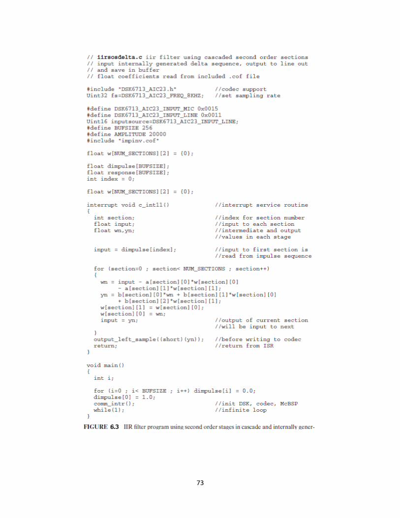
73

74

LAB WORK II: 18. Open project iirsosdelta.pjt by selecting Project →Open and double – clicking on

file iirsosdelta.pjt in folder iirsosdelta. 19. Connect the LINE OUT socket on the DSK to an oscilloscope. 20. Load and run the executable file iirsosdelta.out. 21. Monitor the output (impulse response of the filter) on the scope and make your notes.

The output waveform is shaped both by the IIR filter and by the AIC23 codec reconstruction filter.

22. Using the FFT feature of the scope, capture the magnitude of the frequency response

of the filter. In the frequency domain, the codec reconstruction filter is responsible for the steep roll – off of gain at frequencies above 3500 Hz and the ac coupling of the codec output is responsible for the steep roll - off of gain at frequencies below 100 Hz.

23. Halt the program and select View→ Graph. Set the Graph Properties as indicated in

Figure 6.4 and you should see something similar to the right - hand graph shown in Figure 6.5. You need to set the Graph Properties differently to see something similar to the left - hand graph shown in Figure 6.5.

75

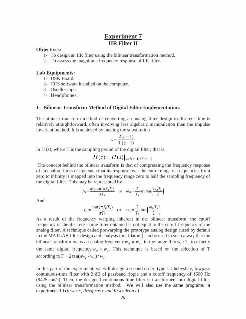
76

Experiment 7 IIR Filter II

Objectives: 1- To design an IIR filter using the bilinear transformation method. 2- To assess the magnitude frequency response of IIR filter.

Lab Equipments:

1- DSK Board. 2- CCS software installed on the computer. 3- Oscilloscope. 4- Headphones.

1- Bilinear Transform Method of Digital Filter Implementation. The bilinear transform method of converting an analog filter design to discrete time is relatively straightforward, often involving less algebraic manipulation than the impulse invariant method. It is achieved by making the substitution

In H (s), where T is the sampling period of the digital filter; that is,

The concept behind the bilinear transform is that of compressing the frequency response of an analog filters design such that its response over the entire range of frequencies from zero to infinity is mapped into the frequency range zero to half the sampling frequency of the digital filter. This may be represented by

And

As a result of the frequency warping inherent in the bilinear transform, the cutoff frequency of the discrete - time filter obtained is not equal to the cutoff frequency of the analog filter. A technique called prewarping the prototype analog design (used by default in the MATLAB filter design and analysis tool fdatool) can be used in such a way that the bilinear transform maps an analog frequency cA ww = , in the range 0 to 2/sw , to exactly the same digital frequency cD ww = . This technique is based on the selection of T according to csc wwwT /)/tan(2 π= . In this part of the experiment, we will design a second order, type 1 Chebyshev, lowpass continuous-time filter with 2 dB of passband ripple and a cutoff frequency of 1500 Hz (9425 rad/s). Then, the designed continuous-time filter is transformed into digital filter using the bilinear transformation method. We will also use the same programs in experiment 10 (iirsos.c, iirsoprns.c and iirsosdelta.c)

77

LAB WORK I: 1. Design the continuous-time filter using the Matlab command:

>> [b,a] = cheby1(2,2,2 * pi * 1500, ’ s ’ ); 2. Draw the frequency response of this filters using the Matlab command:

>> freqs(b,a) 3. Transfer the designed continuous-time filter into digital filter using the Matlab

command: >> [bd,ad] = bilinear(b,a,8000);. Here a sampling frequency of 8000 Hz is assumed. The filter coefficients bz and az are used to create the coefficient filter file bilinear.cof which is then used in the main program iirsos.c.

4. Use Matlab to assess the magnitude frequency response of the digital filter by typing

the command: >> freqz(bz,az). In your report, explain the difference between the designed digital filter and the analog

prototype filter. 5. Launch CCS by double - clicking on its desktop icon. 6. Make a quick test on the DSK. 7. Connect the output of a function generator to the LINE IN socket on the DSK. 8. Connect the LINE OUT socket on the DSK to an oscilloscope. 9. Open file iirsos.c by selecting File →Open and double – clicking on file iirsos.c in

folder iirsos. 10. Change the line that reads #include “impinv.cof” to read #include “bilinear.cof”. 11. Build the project. 12. Load and run the executable file iirsos.out. 13. Construct a table to assess the magnitude frequency response of the filter.

i. Set the output of the function generator to sinusoidal. ii. Change the frequency of the sinusoidal signal at the output of a function

from 100 Hz to 4000 Hz in steps and record the peak value of the signal on the scope.

78

Frequency Peak Value dB value

You will find that the cutoff frequency of the discrete - time filter obtained is not 1500 Hz but 1356 Hz. In addition, you will find that the gain of the analog filter at a frequency of 4500 Hz is equal to the gain of the digital filter at a frequency of 2428 Hz and that the digital frequency 1500 Hz corresponds to an analog frequency of 1702 Hz.

14. Alternatively, we can estimate the frequency response of the digital filter using

Pseudorandom Noise as input. Halt the executable file iirsos.out. 15. Open file iirsosprn.c by selecting File →Open and double – clicking on file

iirsoprns.c in folder iirsosprn. 16. Change the line that reads #include “impinv.cof” to read #include “bilinear.cof”. 17. Build the project. 18. Load and run the executable file iirsosprn.out. 19. Using the FFT feature of the scope, capture the output of program iirsosprn.out,

compare the plot with your results in steps 4 and 13. 2- Estimating the Frequency Response of an IIR Filter Using a Sequence of Impulses as Input ( iirsosdelta).

LAB WORK II: 20. Launch CCS by double - clicking on its desktop icon. 21. Connect the LINE OUT socket on the DSK to an oscilloscope. 22. Open project iirsosdelta.pjt by selecting Project →Open and double – clicking on

file iirsosdelta.pjt in folder iirsosdelta. 23. Edit file iirsosdelta.c and change the line that reads #include “impinv.cof” to read

#include “bilinear.cof”. 24. Build the project.

79

25. Load and run the executable file iirsosdelta.out. 26. Monitor the output (impulse response of the filter) on the scope and make your notes.

The output waveform is shaped both by the IIR filter and by the AIC23 codec reconstruction filter.

27. Using the FFT feature of the scope, capture the magnitude of the frequency response

of the filter. 28. Halt the program and select View→ Graph. Set the Graph Properties as indicated in

Figure 7.1, save the obtained graph and used in your report. 29. You need to set the Graph Properties differently to see the impulse response of the

filter in the time domain.

3- Design of IIR Filters Using MATLAB ’s Filter Design and Analysis Tool MATLAB provides a filter design and analysis tool, fdatool, that makes the design of IIR filter coefficients simple. Coefficients can be exported in direct form II, second order section format and a MATLAB function dsk_sos_iir67() written by the author of the text book can be used to generate coefficient files compatible with the programs (iirsos.c, iirsoprns.c and iirsosdelta.c).

80

LAB WORK III: 30. Start FDATool from the MATLAB command line by typing: >>fdatool. 31. In the Response Type pane, select Lowpass. 32. In the Design Method pane, select IIR, and then select Butterworth 33. For the Filter Order, select Specify order, and then enter 6. 34. Set frequency specifications to Fs to 8000 and Fc to 1500. 35. Click the Design Filter button, you will shortly be able to see the magnitude response

of the designed filter, make your not and save it to use it in your report. 36. Click on Export in the fdatool File menu. 37. Select Workspace, Coefficients, SOS , and G and click Export . 38. At the MATLAB command line, type dsk_sos_iir67(SOS,G) and enter a filename

Butterworth.cof . 39. Launch CCS by double - clicking on its desktop icon. 40. Connect the LINE OUT socket on the DSK to an oscilloscope. 41. Open project iirsosdelta.pjt by selecting Project →Open and double – clicking on

file iirsosdelta.pjt in folder iirsosdelta. 42. Edit file iirsosdelta.c and change the line that reads #include “ impinv.cof ” to read

#include “Butterworth.cof ”. 43. Build the project. 44. Load and run the executable file iirsosdelta.out. 45. Monitor the output (impulse response of the filter) on the scope and make your notes. 46. Using the FFT feature of the scope, capture the magnitude of the frequency response

of the filter. 47. Halt the program and select View→ Graph. Set the Graph Properties as indicated in

Figure 7.1, save the obtained graph and compare it with that in step 35. 48. You need to set the Graph Properties differently to see the impulse response of the

filter in the time domain.

81

Experiment 8 Discrete Time and Fast Fourier Transforms

Objectives:

1- To compute the Discrete Fourier Transform (DTF) of real signal. 2- To compute the Fast Fourier Transform (FFT) of real signal. 3- To estimate the execution time for the DFT and FFT functions

Lab Equipments:

1- DSK Board. 2- CCS software installed on the computer. 3- Oscilloscope. 4- Headphones.

1- DFT of a Sequence of Real Numbers with Output in the

CCS Graphical Display Window ( dft ) This part of the experiment illustrates the DFT of an N - point, real - valued sequence. Program dft.c, listed in Figure 8.1, calculates the complex DFT:

Using Euler ’ s relation to represent a complex exponential

The real and imaginary parts of X (k) are computed by the program:

A structured data type COMPLEX is used by the program to represent the complex valued time - and frequency - domain values of X(k) and x(n). The function dft() has been written such that it replaces the input samples x(n), stored in array samples with their frequency - domain representation X(k). The time - domain sequence x(n) consists of exactly 10 cycles of a real - valued cosine wave (assuming a sampling frequency of 8 kHz, the frequency of the cosine wave is 800 Hz). The DFT of this sequence, X ( k ), is equal to zero for all k , except at k = 10 and at k = 90. These two real values correspond to frequency components at ± 800 Hz. Different time - domain input sequences can be used in the program, most readily by changing the value of the constant TESTFREQ .

82

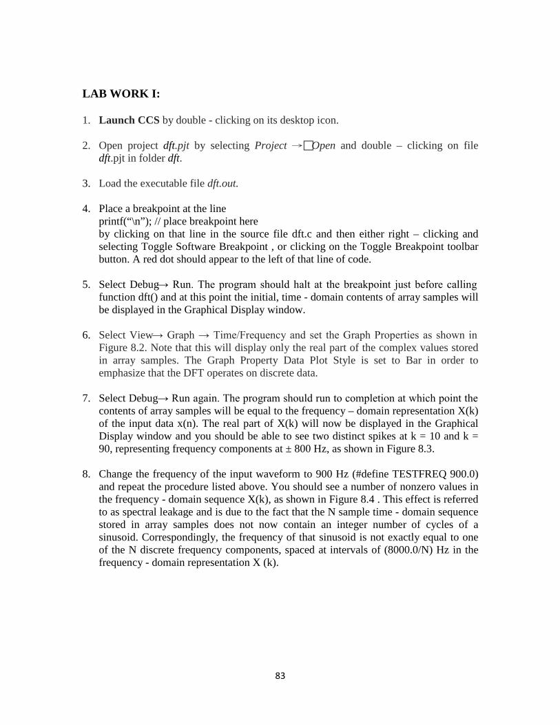
83

LAB WORK I: 1. Launch CCS by double - clicking on its desktop icon. 2. Open project dft.pjt by selecting Project →Open and double – clicking on file

dft.pjt in folder dft. 3. Load the executable file dft.out. 4. Place a breakpoint at the line

printf(“\n”); // place breakpoint here by clicking on that line in the source file dft.c and then either right – clicking and selecting Toggle Software Breakpoint , or clicking on the Toggle Breakpoint toolbar button. A red dot should appear to the left of that line of code.

5. Select Debug→ Run. The program should halt at the breakpoint just before calling function dft() and at this point the initial, time - domain contents of array samples will be displayed in the Graphical Display window.

6. Select View→ Graph → Time/Frequency and set the Graph Properties as shown in

Figure 8.2. Note that this will display only the real part of the complex values stored in array samples. The Graph Property Data Plot Style is set to Bar in order to emphasize that the DFT operates on discrete data.

7. Select Debug→ Run again. The program should run to completion at which point the

contents of array samples will be equal to the frequency – domain representation X(k) of the input data x(n). The real part of X(k) will now be displayed in the Graphical Display window and you should be able to see two distinct spikes at k = 10 and k = 90, representing frequency components at ± 800 Hz, as shown in Figure 8.3.

8. Change the frequency of the input waveform to 900 Hz (#define TESTFREQ 900.0)

and repeat the procedure listed above. You should see a number of nonzero values in the frequency - domain sequence X(k), as shown in Figure 8.4 . This effect is referred to as spectral leakage and is due to the fact that the N sample time - domain sequence stored in array samples does not now contain an integer number of cycles of a sinusoid. Correspondingly, the frequency of that sinusoid is not exactly equal to one of the N discrete frequency components, spaced at intervals of (8000.0/N) Hz in the frequency - domain representation X (k).

84

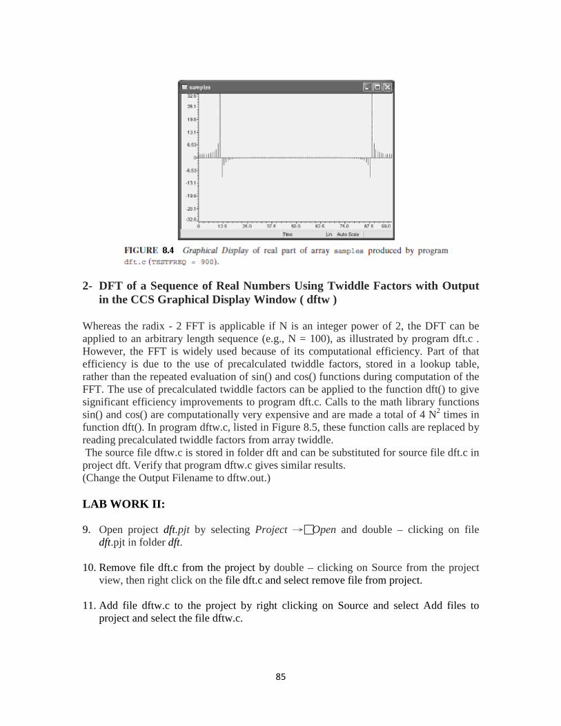
85

2- DFT of a Sequence of Real Numbers Using Twiddle Factors with Output

in the CCS Graphical Display Window ( dftw )

Whereas the radix - 2 FFT is applicable if N is an integer power of 2, the DFT can be applied to an arbitrary length sequence (e.g., N = 100), as illustrated by program dft.c . However, the FFT is widely used because of its computational efficiency. Part of that efficiency is due to the use of precalculated twiddle factors, stored in a lookup table, rather than the repeated evaluation of sin() and cos() functions during computation of the FFT. The use of precalculated twiddle factors can be applied to the function dft() to give significant efficiency improvements to program dft.c. Calls to the math library functions sin() and cos() are computationally very expensive and are made a total of 4 N2 times in function dft(). In program dftw.c, listed in Figure 8.5, these function calls are replaced by reading precalculated twiddle factors from array twiddle. The source file dftw.c is stored in folder dft and can be substituted for source file dft.c in project dft. Verify that program dftw.c gives similar results. (Change the Output Filename to dftw.out.)

LAB WORK II: 9. Open project dft.pjt by selecting Project →Open and double – clicking on file

dft.pjt in folder dft. 10. Remove file dft.c from the project by double – clicking on Source from the project

view, then right click on the file dft.c and select remove file from project. 11. Add file dftw.c to the project by right clicking on Source and select Add files to

project and select the file dftw.c.

86

12. Select Project→ Build Options. In the Compiler tab in the Basic category set the Opt Level to Function(− o2) and in the Linker tab set the Output Filename to .\Debug\dftw.out .

87

13. Build the project. 14. Load the executable file dftw.out. 15. Place a breakpoint at the line

printf(“\n”); // place breakpoint here by clicking on that line in the source file dftw.c and then either right – clicking and selecting Toggle Software Breakpoint , or clicking on the Toggle Breakpoint toolbar button. A red dot should appear to the left of that line of code.

16. Select Debug→ Run. The program should halt at the breakpoint just before calling

function dftw() and at this point the initial, time - domain contents of array samples will be displayed in the Graphical Display window.

17. Select View→ Graph → Time/Frequency and set the Graph Properties as shown in

Figure 8.2. Note that this will display only the real part of the complex values stored in array samples. The Graph Property Data Plot Style is set to Bar in order to emphasize that the DFT operates on discrete data.

18. Select Debug→ Run again. The program should run to completion at which point the

contents of array samples will be equal to the frequency – domain representation X(k) of the input data x(n). The real part of X(k) will now be displayed in the Graphical Display window and you should be able to see two distinct spikes at k = 10 and k = 90, representing frequency components at ± 800 Hz, as shown in Figure 8.3.

19. Change the frequency of the input waveform to 900 Hz (#define TESTFREQ 900.0)

and repeat the procedure listed above. You should see a number of nonzero values in the frequency - domain sequence X(k), as shown in Figure 8.4 . This effect is referred to as spectral leakage and is due to the fact that the N sample time - domain sequence stored in array samples does not now contain an integer number of cycles of a sinusoid. Correspondingly, the frequency of that sinusoid is not exactly equal to one of the N discrete frequency components, spaced at intervals of (8000.0/N) Hz in the frequency - domain representation X (k).

3- Estimating Execution Times for DFT and FFT Functions (fft) The computational expense of function dft() can be illustrated using Code Composer’s Profile Clock. In this part of the experiment, the functions dft() and dftw() used in Lab Work I and II are compared with a third function, fft() , which implements the FFT in C.

LAB WORK III: 20. Edit the lines in programs dft.c and dftw.c that read

#define N 100 to read #define N 128

88

21. Ensure that source file dft.c and not dftw.c is present in the project. 22. Select Project→ Build Options. In the Compiler tab in the Basic category set the Opt

Level to Function (− o2) and in the Linker tab set the Output Filename to .\Debug\dft.out .

23. Build the project and load dft.out. 24. Open source file dft.c by double - clicking on its name in the Project View window

and set breakpoints at the lines dft(samples); and printf(“done!\n”); .

25. Select Profile → Clock → Enable. 26. Select Profile → Clock View. A small clock icon and the number of processor

instruction cycles that the Profile Clock has counted should appear in the bottom right - hand corner of the Code Composer window.

27. Run the program. It should halt at the first breakpoint. 28. Reset the Profile Clock by double - clicking on its icon in the bottom right – hand

corner of the CCS window. 29. Run the program. It should stop at the second breakpoint. The number of instruction

cycles counted by the Profile Clock gives an indication of the computational expense of executing function dft().

30. Repeat the preceding experiment (step 22 to step 27) substituting file dftw.c for file

dft.c. 31. Finally, repeat the preceding experiment (step 22 to step 27) using file fft.c (also

stored in folder dft) (see Figure 8.6). This program computes the FFT using a function written in C and defined in the file fft.h (Figure 8.7). The advantage, in terms of execution time, of the FFT over the DFT should increase with the number of points, N, used. Repeat this example using different values of N (e.g., 256 or 512).

89

N=128 N=256 N=512 Number of

Instruction Cycles

Execution Time

Number of Instruction

Cycles

Execution Time

Number of Instruction

Cycles

Execution Time

dft.c

dftw.c

fft.c

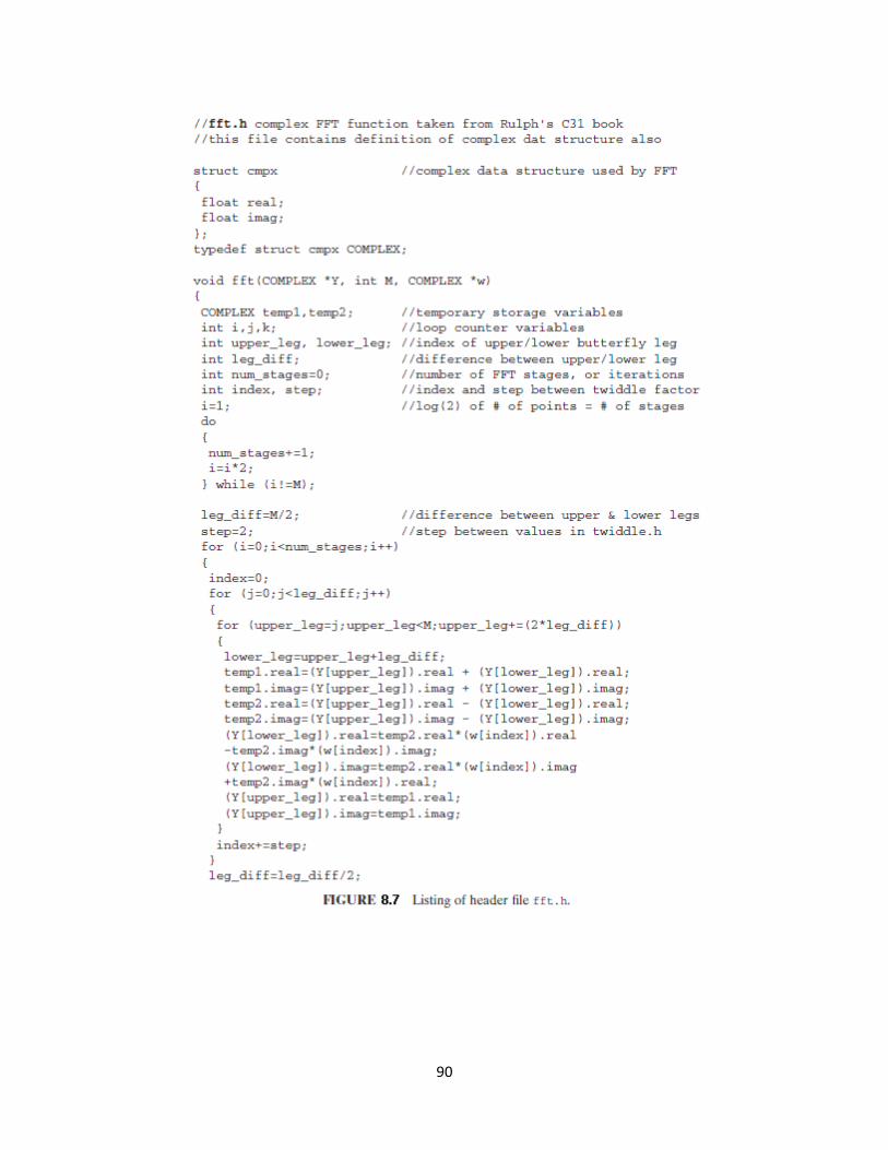
90