Jordan Journal of Mathematics and Statistics - …journals.yu.edu.jo/jjms/Issues/vol2No12009/JJMS...

The Hashemite Kingdom of Jordan Yarmouk University

Jordan Journal of Mathematics and Statistics An International Research Journal

Volume 2, No. 1, June 2009, Rajab 1430 H



Jordan Journal of Mathematics and Statistics (JJMS): An International Peer-Reviewed Research Journal established by the Higher Research Committee, Ministry of Higher Education and Scientific Research, Jordan, and published quarterly by the Deanship of Research and Graduate Studies, Yarmouk University, Irbid, Jordan. EDITOR-IN-CHIEF: Mashhoor A. Al-Refai

Department of Mathematics, Yarmouk University, Irbid, Jordan. Current Address:Vice President, Yarmouk University, Irbid, Jordan.

E-mail: [email protected] EDITORIAL SECRETARY: Mrs. Manar M. Malkawi, Deanship of Research and Graduate Studies EDITORIAL BOARD:

Nabil T. Shawagfeh Department of Mathematics, University of Jordan, Amman, Jordan.

Current Address: President, Al-al-Bayt University, Al-Mafraq, Jordan. E-mail: [email protected] Mufid M. Azzam Department of Mathematics, University of Jordan, Amman, Jordan. E-mail: [email protected] Ahmed T. Alawneh Department of Mathematics, University of Jordan, Amman, Jordan. E-mail: [email protected] Bassam Y. Al-Nashef Department of Mathematics, Yarmouk University, Irbid, Jordan. E-mail: [email protected] Fuad A. Kittaneh Department of Mathematics, University of Jordan, Amman, J ordan. E-mail: [email protected] Abdulla M. Al-Jarrah Department of Mathematics, Yarmouk University, Irbid, Jordan. E-mail: [email protected]

Scientific Editor: Abdulla M. Al-Jarrah, Department of Mathematics, Yarmouk University. Manuscripts should be submitted to:

Prof. Mashhoor A. Al-Refai

Editor-in-Chief, Jordan Journal of Mathematics and Statistics Deanship of Research and Graduate Studies

Yarmouk University-Irbid-Jordan Tel. 00 962 2 7211111 Ext. 2026

E-mail: [email protected] Website: http://jjms.yu.edu.jo

Jordan Journal of

Mathematics and Statistics An International Research Journal


INTERNATIONAL ADVISORY BOARD

Abu-Dayyeh, Walid Ahmad DOMAS, College of Science, P.O. Box 36,Sultan Qaboos University, Al-Khod 123,Oman E-mail: [email protected] Ahmad, M.K. Dept. of Mathematics, Aleppo University, Syria Email: [email protected] Aldroubi, Akram Dept. of Mathematics,Vanderbilt University, Nashville, TN 37240, USA Email: [email protected] Baddour, Hassan Dept. of Mathematics, Tishreen University, Syria E-mail: [email protected] Corsini, Piergiulio University of Udine, Italy E-mail: [email protected] De Malafosse, Bruno LMAH, Université du Havre, BP 4006 IUT Le Havre, 76610 Le Havre, France Email: [email protected] Duflot, Jeanne 101 Weber Building, Colorado State University Fort Collins, CO 80523-1874, USA E-mail: [email protected] Ganster, Maximilian Dept. of Mathematics, Graz University of Technology, Steyrergasse 30, A-8010 Graz, Austria E-mail: [email protected] Gowrisankaran, Kohur Dept. of Mathematics & Statistics, McGill University, 805 Sherbrooke W., Montreal Qc H3A 2K6,Canada E-mail: [email protected] Hajja, Mowaffaq Abdulla Dept. of Mathematics, Yarmouk University, Irbid, Jordan E-mail: [email protected] Hailat, Mohammad Chair of Mathematical Sciences Dept., University of South Carolina, Aiken, 471 University Parkway, Aiken, SC 29801, USA Email: [email protected] Hamdan, Mohammed Senior Advisor, Arab Open University, P.O. Box 1339, Amman 11953, Jordan E-mail: [email protected] Ismail, Mourad E.H. Department of Mathematics, University of Central Florida, Orlando, FL 32816,USA E-mail: [email protected] Jain, Pawan F.N.A.Sc. Dept. of Mathematics, University of Delhi,Delhi 110 007, India Email: [email protected] Kabbaj, Salah-Eddine Dept. of Mathematical Sciences, King Fahd University of Petroleum & Minerals (KFUPM), PO Box 5046, Dhahran 31261, Saudi Arabia Email: [email protected] Kang, Ming-Chang Department of Mathematics,National Taiwan University,Taipei, Taiwan Email: [email protected]

Kiryakova, Virginia Institute of Mathematics and Informatics - Bulgarian Academy of Sciences Acad. G. Bontchev Street, Block 8, Sofia 1113, Bulgaria E-mail: virginia@ diogenes.bg Kokilashvili, Vakhtang A. Razmadze Mathematical Institute, Georgian Academy of Sciences, 1, Aleksidze Str.,Tbilisi, Georgia Email: [email protected] Lau, Ka-Sing Dept. of Mathematics, Chinese University of Hong Kong, Shatin, Hong Kong E-mail: [email protected] Lu, Shanzhen Dept. of Mathematical Sciences, Beijing Normal University, Beijing 100875, P.R. China E-mail: [email protected] Madi, Mohammad Asst. Dean for Research, College of Business & Economics, Internal Funding Unit, Research Affairs, United Arab Emirates University, UAE E-mail: [email protected] Malkowsky, Eberhard Jaegerschneise 26, D-35440 Linden l Forst, Germany E-mail: [email protected] Manfredi, Juan J. Dept. of Mathematics, University of Pittsburg, Pittsburg, PA 15260, USA Email: [email protected] Martini, Horst Chair of the Faculty of Geometry Mathematics Technical University of Chemnitz, 09107 Chemnitz,Germany E-mail: [email protected] Miranda, Rick Dean of Natural Sciences, Colorado State University, Campus Delivery – 1801, Fort Collins, CO 80523-1801, USA E-mail: [email protected] Mullen, Gary L. Department of Mathematics, The Pennsylvania State University, University Park, PA 16802, Phone: +1 814 865 2312 E-mail: [email protected] Nakkar, Hassan College of Science, Dept. of Mathematics, Al-Qassim University, P.O. Box 237, Buraidah 81999, Saudi Arabia E-mail: [email protected] Nashed, Zuhair Dept. of Mathematics, 507 Mathematics and Physics Building, University of Central Florida, Orlando, FL 32816-1364, USA E-mail: [email protected] Pourahmadi, Mohsen Division of Statistics, Northern Illinois University, DeKalb, Ill., 60115, USA Tel: +1 815 753 6829, Fax: 1 815 753 6776 Rakocevic, Vladimir Faculty of Mathematics & Sciences, University of Nis, Visegradska 33, 18000 Nis, Serbia Email: [email protected] Vougioklis, Thomas Dept. of Mathematics, Democritos University of Thrace, Greece E-mail: [email protected] Zayed, Ahmed I. Professor and Chair, Dept. of Mathematical Sciences, Depaul University, 2320 N. Kenmore Ave, SAC 524, Chicago, Ill 60614, USA Email: [email protected]

Scope and Description

Jordan Journal of Mathematics and Statistics (JJMS) is an international quarterly peer-reviewed research journal issued by the Higher Scientific Research Committee, Ministry of Higher Education and Scientific Research, Amman, Jordan. JJMS is published by the Deanship of Research and Graduate Studies, Yarmouk University, Irbid, Jordan. The Journal endeavors to publish significant original research articles in all areas of Pure Mathematics, Applied Mathematics, Pure Statistics , Applied Statistics and other related areas. Survey Papers and short communications will also be considered for publication.

Instructions to Authors

Instructions to authors concerning manuscript organization and format apply to hardcopy submission by mail, and also to electronic online submission via the Journal homepage website (http://jjms.yu.edu.jo).

Manuscript Submission

To submit an article for publication in the JJMS, an author should send a hard copy or an electronic file of the manuscript as a single document including tables and figures. This means it should be one Microsoft word file …(a widely acceptable format e.g. PDF, LATEX/ S.W. preferred)and not a zipped file containing different files for text, tables, etc to:

Editor in chief :Prof. Mashhoor Al-Refai Jordan Journal of Mathematics and statistics Deanship of Research and Graduate Studies

JORDANIrbid –Yarmouk University Tel: 00962-2-7211111 Ext. 2026

Fax: 00962-2-7211121 E-mail: [email protected]

Organization of the Manuscript

Manuscripts must be written in English or Arabic (Manuscripts submitted in Arabic should be accompanied by an abstract and keywords in English).

There are no page charges to individuals or institutions for contributions. All manuscripts will be reviewed. The author should adhere to the following order of presentation: article title, author(s), full address (es)

and e-mail, abstract, current mathematics subject classifications and keywords, main text, acknowledgement and references.

Acknowledgments: Acknowledgments, including those for grant and financial support, should be typed in one paragraph directly preceding the References section.

References: References should be given in alphabetical order according to the surnames of the authors at

the end of the paper. The following style should be used : - G. Köthe (1969), Topological vector spaces I, Springer-Verlag. - D.P.Blecher and V.I.Paulsen, Tensor products of operator spaces, J. Funct. Anal.

99(1991), 262-292.

Reprints and Proofs

Authors will receive the first proofs for necessary corrections (no alterations or corrections, except printing errors will normally be accepted at this point), which should be retuned within two weeks of receipt. Authors will receive one copy of the issue in which their work appears and twenty (20) offprint free of charge.

Copyright

Submission is an admission by the authors that the manuscript has neither been previously published nor is being considered for publication elsewhere. A statement transferring copyright from the authors to Yarmouk University is required before the manuscript can be accepted for publication. The necessary form for such transfer is supplied by the Editor-in-Chief with the article proofs. Reproduction of any part of the contents of a published work is forbidden without a written permission by the Editor-in-Chief.

Disclaimer

Opinions expressed in this journal are those of the authors and do not necessarily reflect the opinions of the editorial board , the university, the policy of the Higher Scientific Research Committee or the Ministry of Higher Education and Scientific Research.

هيئة التحرير أو الجامعة أو سياسة اللجنـة العليـا للبحـث العلمـي أو آراءما ورد في هذه المجلة يعبر عن اراء المؤلفين وال يعكس بالضرورة " "وزارة التربية والتعليم العالي والبحث العلمي

The Hashemite Kingdom of Jordan Yarmouk University





TABLE of CONTENTS

Fractional Calculus Operators Associated with a Subclass of Uniformly Convex Functions G. Murugusundaramoorthy and R. Themangani

1

Some Properties of Unisrially Embedding of Subgroups of P-Groups Hassan Naraghi

11

Homotopy Analysis Method for Delay-Integro-Differential Equations Edris Rawashdeh, H. M. Jaradat and Fadi Awawdeh

15

An Alternative Proof of the Friendship Theorem Mohammad Bataineh

25

Some Applications of the Co-Hyponormal Operators Mohammad Rashid and Basem Masaedeh

33

A Prey-Predator Model with cover for the Prey and An Alternative Food for the Predator and Constant Harvesting of Both the Species K. Lakshimi Narayan and N. Pattabhiramacharyulu

43

Jordan Journal of Mathematics and Statistics (JJMS) 2009, 2(1), 1-10.

FRACTIONAL CALCULUS OPERATORS ASSOCIATEDWITH A SUBCLASS OF UNIFORMLY CONVEX

FUNCTIONS

G.MURUGUSUNDARAMOORTHY AND R.THEMANGANI

Abstract. Making use of fractional calculus operator, we define a new subclass ofuniformly convex functions with negative coefficients. Characterization property, ex-treme points, distortion bounds, the results on Integral transform and sharp integralmeans inequalities for the function class are determined.

1. Introduction and Preliminaries

Denote by A the class of functions of the form

(1.1) f(z) = z +∞∑

n=2

anzn

which are analytic in the unit disc U = z : |z| < 1.. Denote by S the subclass ofA consisting of functions normalized by f(0) = 0 = f ′(0) − 1 which are univalent in Uand ST and CV the subclasses of S of starlike and convex respectively. Also denote thesubclass T consisting of functions in S which are univalent in U and of the form

(1.2) f(z) = z −∞∑

n=2

anzn, (an ≥ 0)

The class T was introduced and studied by Silverman [16].A function f(z) is uniformly convex (uniformly starlike) in 4 if f(z) is in CV (ST )

and has the property that for every circular arc γ contained in 4, with center ξ also in4, the arc f(γ) is convex (starlike) with respect to f(ξ). The class of uniformly convexfunctions is denoted by UCV and the class of uniformly starlike functions by UST (fordetails see [4, 5]). It is well known from [9, 14] that

f ∈ UCV ⇔∣∣∣∣zf ′′

(z)

f ′(z)

∣∣∣∣ ≤ Re

1 +

zf′′(z)

f ′(z)

.

1991 Mathematics Subject Classification. Primary: 30C45; Secondary: 30C50.Key words and phrases. Classes of Univalent functions, convex functions, starlike functions, uni-

formly convex functions, fractional derivatives, fractional integral, integral means.Copyright c© Deanship of Research and Graduate Studies, Yarmouk University, Irbid, Jordan.

Received : Aug. 31,2008 Accepted : June 16,2009.1

2 G.MURUGUSUNDARAMOORTHY AND R.THEMANGANI

In [14], Rønning introduced a new class of starlike functions related to UCV and definedas

f ∈ Sp ⇔∣∣∣∣zf ′

(z)

f(z)− 1

∣∣∣∣ ≤ Re

zf

′(z)

f(z)

.

Note that f(z) ∈ UCV ⇔ zf ′(z) ∈ Sp . Further, Rønning [15], generalized the class Sp

by introducing a parameter γ, −1 ≤ γ < 1,

f ∈ Sp(γ) ⇔∣∣∣∣zf ′

(z)

f(z)− 1

∣∣∣∣ ≤ Re

zf

′(z)

f(z)− γ

.

We recall the following definitions of the classical operators of fractional calculus,adopted for working in classes of analytic functions in complex plane by Owa [11] andSrivastava and Owa [18],etc.as follows.

Definition 1.1. [11] Let the function f(z) be analytic in a simply - connected region ofthe z− plane containing the origin. The fractional integral of f of order µ is defined by

(1.3) D−µz f(z) =

1

Γ(µ)

z∫0

f(ξ)

(z − ξ)1−µdξ, µ > 0,

where the multiplicity of (z − ξ)1−µ is removed by requiring log(z − ξ) to be real whenz − ξ > 0.

Definition 1.2. [11] The fractional derivatives of order µ, is defined for a function f(z),by

(1.4) Dµz f(z) =

1

Γ(1− µ)

d

dz

z∫0

f(ξ)

(z − ξ)µdξ, 0 ≤ µ < 1,

where the function f(z) is constrained, and the multiplicity of the function (z − ξ)−µ isremoved as in Definition 1.1.

Definition 1.3. [11] Under the hypothesis of Definition 1.2, the fractional derivative oforder n + µ is defined by

(1.5) Dn+µz f(z) =

dn

dznDµ

z f(z), (0 ≤ µ < 1 ; n ∈ N0).

With the aid of the above definitions, and their known extensions involving fractionalderivative and fractional integrals, Srivastava and Owa [18] introduced the operator Ωδ

(δ ∈ R; δ 6= 2, 3, 4, . . . ) : A → A defined by

Ωδf(z) = Γ(2− δ)zδDδzf(z),

Ωδf(z) = z +∞∑

n=2

Φ(n, δ)anzn(1.6)

where

Φ(n, δ) =Γ(n + 1)Γ(2− δ)

Γ(n + 1− δ).(1.7)

FRACTIONAL CALCULUS OPERATORS ASSOCIATED WITH A SUBCLASS OF UCV 3

Motivated by the earlier works of Altintas et al.[2, 3], Owa[12] , and Raina andSrivastava[13]) we define a subclass of uniformly convex functions based on fractionalcalculus operator .

For 0 ≤ γ < 1, 0 ≤ α < 2 and 0 ≤ β < 2, we let UCV (α, β, γ) be the class of functionsf ∈ S satisfying the inequality

(1.8) Re

Ωαf(z)

Ωβf(z)− γ

>

∣∣∣∣Ωαf(z)

Ωβf(z)− 1

∣∣∣∣ , z ∈ U.

We also let TUCV (α, β, γ) = UCV (α, β, γ) ∩ T.The main object of the present paper is to investigate some coefficient estimates,

extreme points, distortion bounds and results on integral transforms for the subclassTUCV (α, β, γ). We also obtain integral means inequality for higher order fractionalderivative and fractional integrals of functions belonging to this class.

2. Main Results

In this section we obtain a necessary and sufficient condition for functions f(z) in theclass TUCV (α, β, γ).

Theorem 2.1. A function f(z) of the form (1.1) is in UCV (α, β, γ) if

(2.1)∞∑

n=2

[2Φ(n, α)− (1 + γ)Φ(n, β)]

1− γ|an| ≤ 1,

0 ≤ α < 2, 0 ≤ β < 2 and 0 ≤ γ < 1.

Theorem 2.2. A function f(z) of the form (1.2) is in the class TUCV (α, β, γ) if andonly if

∞∑n=2

[2Φ(n, α)− (1 + γ)Φ(n, β)] an ≤ 1− γ,

0 ≤ α < 2, 0 ≤ β < 2 and 0 ≤ γ < 1.

The proofs of Theorem 2.1 and Theorem 2.2, are much akin to the proofs of theoremsgiven in [10], hence we omit the details.

Corollary 2.3. Let a function f(z) defined by (1.2) belong to the class TUCV (α, β, γ).Then

an ≤1− γ

[2Φ(n, α)− (1 + γ)Φ(n, β)], n ≥ 2.

The equality is attained for the function f(z) given by

(2.2) f(z) = z − 1− γ

[2Φ(n, α)− (1 + γ)Φ(n, β)]zn, n ≥ 2.

Theorem 2.4. (Extreme Points) Let the function f(z) defined by (1.2) satisfy (1.8).

Define f1(z) = z and fn(z) = z − zn

Bn(n = 2, 3, . . . ), where Bn = [2Φ(n,α)−(1+γ)Φ(n,β)]

(1−γ).


Then f ∈ TUCV (α, β, γ) if and only if f(z) can be expressed as f(z) =∞∑

n=1

λnfn(z),

where∞∑

n=1

λn = 1 and λn ≥ 0.

Proof. Suppose f(z) =∞∑

n=1

λnfn(z) = z −∞∑

n=2

λn

BnBn =

∞∑n=2

λn = 1 − λ1 ≤ 1. Thus

f ∈ TUCV (α, β, γ).

Conversely, suppose f ∈ TUCV (α, β, γ). Since |an| ≤ 1Bn

, (n = 2, 3, . . . ), we may set

λn = Bn|an|, (n = 2, 3, . . . ) and λ1 = 1−∞∑

n=2

λn. Then f(z) =∞∑

n=1

λnfn(z).

This completes the proof.

Theorem 2.5. Let 0 ≤ α < 2, β ≤ α and 0 ≤ γ < 1. If f(z) ∈ TUCV (α, β, γ), then

|z| − (1− γ)(2− α)(2− β)

2[2(2− β)− (1 + γ)(2− α)]|z|2 ≤ |f(z)| ≤ |z|+ (1− γ)(2− α)(2− β)

2[2(2− β)− (1 + γ)(2− α)]|z|2

for z ∈ U.

Proof. Let 0 ≤ α < 2, β ≤ α and 0 ≤ γ < 1 and let f(z) ∈ TUCV (α, β, γ). Then, byvirtue of Theorem 2.2, we obtain

[2Φ(2, α)− (1 + γ)Φ(2, β)]∞∑

n=2

an ≤∞∑

n=2

[2Φ(n, α)− (1 + γ)Φ(n, β)]an ≤ 1− γ

where Φ(n, α) and Φ(n, β) are given by (1.7). This readily yields

(2.3)∞∑

n=2

an ≤1− γ

[2Φ(2, α)− (1 + γ)Φ(2, β)]=

(1− γ)(2− α)(2− β)

2[2(2− β)− (1 + γ)(2− α)]

Using (1.2) and (2.3) we obtain

|f(z)| ≥ |z| − |z|2∞∑

n=2

an

≥ |z| − (1− γ)(2− α)(2− β)

2[2(2− β)− (1 + γ)(2− α)]|z|2

and

|f(z)| ≤ |z|+ |z|2∞∑

n=2

an

≤ |z|+ (1− γ)(2− α)(2− β)

2[2(2− β)− (1 + γ)(2− α)]|z|2

which completes the proof of Theorem 2.5.

Using the definitions of fractional integral operator and fractional derivative operator,we obtain distortion bounds for the class TUCV (α, β, γ).


Theorem 2.6. Let the function f(z) defined by (1.2) be in the class TUCV (α, β, γ).Then we have∣∣D−µ

z (Ωαf(z))∣∣ ≥ |z|1+µ

Γ(2 + µ)

1− 2(2− β)(1− γ)|z|

(2 + µ)[2(2− β)− (1 + γ)(2− α)]

and ∣∣D−µ

z (Ωαf(z))∣∣ ≤ |z|1+µ

Γ(2 + µ)

1 +

2(2− β)(1− γ)|z|(2 + µ)[2(2− β)− (1 + γ)(2− α)]

for 0 ≤ α < 2, β ≤ α and 0 ≤ γ < 1; z ∈ U.

Proof. Define the function F (z) by

F (z) = Γ(2 + µ)z−µD−µz (Ωαf(z))

= Γ(2 + µ)z−µD−µz [Γ(2− µ)zαDα

z f(z)]

= z −∞∑

n=2

Γ(n + 1)Γ(n + 1)Γ(2− α)Γ(2 + µ)

Γ(n + 1− α)Γ(n + 1 + µ)znan

= z −∞∑

n=2

Ψ(n)anzn

where

Ψ(n) =Γ(n + 1)Γ(n + 1)Γ(2− α)Γ(2 + µ)

Γ(n + 1− α)Γ(n + 1 + µ)(n ≥ 2).

It is easy to see that

0 < Ψ(n) ≤ Ψ(2) =4

(2− α)(2 + µ).(2.4)

Using Theorem 2.2, we have,

4

2− α− (1 + γ)

2

2− β

∞∑n=2

an ≤∞∑

n=2

[2Φ(n, α)− (1 + γ)Φ(n, β)] an ≤ 1− γ

∞∑n=2

an ≤(2− α)(2− β)(1− γ)

2[2(2− β)− (1 + γ)(2− α)].(2.5)

Using (2.4) and (2.5) we can see that,

|F (z)| ≥ |z| −Ψ(2)|z|2∞∑

n=2

an

≥ |z| − 2(2− β)(1− γ)

(2 + µ)[2(2− β)− (1 + γ)(2− α)]|z|2


and

|F (z)| ≤ |z|+ Ψ(2)|z|2∞∑

n=2

an

≤ |z|+ 2(2− β)(1− γ)

(2 + µ)[2(2− β)− (1 + γ)(2− α)]|z|2.

Which proves the assertion of Theorem 2.6.

Theorem 2.7. Let the function f(z) defined by (1.2) be in the class TUCV (α, β, γ).Then we have

|Dµz (Ωαf(z))| ≥ |z|1−µ

Γ(2− µ)

1− 2(2− β)(1− γ)|z|

(2− µ)[2(2− β)− (1 + γ)(2− α)]

and

|Dµz (Ωαf(z))| ≤ |z|1−µ

Γ(2− µ)

1 +

2(2− β)(1− γ)|z|(2− µ)[2(2− β)− (1 + γ)(2− α)]

for 0 ≤ α < 2, β ≤ α, 0 ≤ γ < 1 and 0 ≤ µ < 1; z ∈ U.

Theorem 2.8. Let the function f(z) defined by (1.2) be in the class TUCV (α, β, γ).Then we have∣∣D1+µ

z (Ωαf(z))∣∣ ≥ |z|−µ

Γ(1− µ)

1− 2(2− β)(1− γ)|z|

(1− µ)[2(2− β)− (1 + γ)(2− α)]

and ∣∣D1+µ

z (Ωαf(z))∣∣ ≤ |z|−µ

Γ(1− µ)

1 +

2(2− β)(1− γ)|z|(1− µ)[2(2− β)− (1 + γ)(2− α)]

for 0 ≤ α < 2, β ≤ α, 0 ≤ γ < 1 and 0 ≤ µ < 1; z ∈ U\0.

3. Integral Means for the Class

Recently Ahuja and Jahangiri [1], Kim and Choi [6], Murugusundaramoorthy andThomas Rosy [10] and Silverman [17] had obtained sharp integral means inequalities forunivalent functions with negative coefficients. In this section we obtain some results onintegral means inequalities.

We recall first the concept of subordination between analytic functions and a subor-dination theorem of Littlewood [8] .

Given two functions f(z) and g(z) which are analytic in ∆ with f(0) = g(0). Thefunction f(z) is said to subordinate to g(z) in ∆ if there exists a function w(z) analyticin ∆ with w(0) = 0 and |w(z)| < 1, z ∈ ∆ such that f(z) = g(w(z)), z ∈ ∆. We denotethe subordination by f(z) ≺ g(z).


Theorem 3.1. [8] If the functions f(z) and g(z) are analytic in ∆ with g(z) ≺ f(z)then

(3.1)

2π∫0

∣∣g(reiθ)∣∣η dθ ≤

2π∫0

∣∣f(ηeiθ)∣∣η dθ, η > 0, 0 < r < 1.

Theorem 3.2. Let η > 0 and f2(z) is defined by (2.2). If f(z) ∈ TUCV (α, β, γ) thenfor z = reiθ and 0 < r < 1

(3.2)

2π∫0

∣∣D1+δz f(z)

∣∣γ dθ ≤2π∫0

∣∣D1+δz f2(z)

∣∣γ dθ, γ > 0, 0 ≤ δ < 1.

Proof. By virtue of the fractional derivative formula given and defined in Definition (1.3),we find from (1.2) that

D1+δz f(z) =

z−δ

Γ(1− δ)

[1−

∞∑n=2

Γ(1− δ)Γ(n + 1)

Γ(n− δ)anz

n−1

]

=z−δ

Γ(1− δ)

[1−

∞∑n=2

Γ(1− δ)n!

(n− 2)!Ψ(n)anz

n−1

]where

Ψ(n) =Γ(n− 1)

Γ(n− δ), (0 ≤ δ < 1; n ≥ 2).

Since Ψ(n) is decreasing function of n we have

0 < Ψ(n) ≤ Ψ(2) =1

Γ(2− δ)(0 ≤ δ < 1; n ≥ 2).

Similarly

D1+δz f2(z) =

z−δ

Γ(1− δ)

[1− Γ(1− δ)Γ(3)

B2Γ(2− δ)z

]where B2 as in Theorem 2.2. For z = reiθ and 0 < r < 1, we must show that

2π∫0

∣∣∣∣∣1−∞∑

n=2

Γ(1− δ)n!

(n− 2)!Ψ(n)anz

n−1

∣∣∣∣∣η

dθ ≤2π∫0

∣∣∣∣1− Γ(1− δ)Γ(3)

B2Γ(2− δ)z

∣∣∣∣η dθ,

η > 0, 0 ≤ δ < 1. Thus by Theorem 3.1 and applying Theorem 2.2 it sufficies to showthat

1−∞∑

n=2

Γ(1− δ)n!

(n− 2)!Ψ(n)anz

n−1 ≺ 1− Γ(1− δ)Γ(3)

B2Γ(2− δ)w(z)


where

|w(z)| =

∣∣∣∣∣B2Γ(2− δ)

Γ(1− δ)

∞∑n=2

Γ(1− δ)n!

(n− 2)!Ψ(n)anz

n−1

∣∣∣∣∣=

∣∣∣∣∣B2

∞∑n=2

anzn−1

∣∣∣∣∣ ≤ |z|∞∑

n=2

Bnan < 1

by means of the hypothesis of Theorem. In light of the above inequality we have thesubordination (3.2) which evidently proves the theorem.

4. Integral Transform of the class TUCV (α, β, γ)

For f ∈ A we define the integral transform

Vλ(f)(z) =

1∫0

λ(t)f(tz)

tdt,

where λ is a real valued, non-negative weight function normalized so that∫ 1

0λ(t)dt = 1.

Since special cases of λ(t) are particularly interesting such as λ(t) = (1 + c)tc, c > −1,for which Vλ is known as the Bernardi operator, and

λ(t) =(c + 1)δ

λ(δ)tc(

log1

t

)δ−1

, c > −1, δ ≥ 0

which gives the Komatu operator( see [7]).First we show that the class TUCV (α, β, γ) is closed under Vλ(f).

Theorem 4.1. Let f ∈ TUCV (α, β, γ). Then Vλ(f) ∈ TUCV (α, β, γ).

Proof. By definition, we have

Vλ(f)(z) =(c + 1)δ

λ(δ)

1∫0

(−1)δ−1tc(log t)δ−1

(z −

∞∑n=2

anzntn−1

)dt

=(−1)δ−1(c + 1)δ

λ(δ)lim

r→0+

1∫r

tc(log t)δ−1

(z −

∞∑n=2

anzntn−1

)dt

.

A simple calculation gives

Vλ(f)(z) = z −∞∑

n=2

(c + 1

c + n

)δ

anzn.

We need to prove that

(4.1)∞∑

n=2

[2Φ(n, α)− (1 + γ)Φ(n, β)]

(1− γ)

(c + 1

c + n

)δ

an ≤ 1.


On the other hand by Theorem 2.2, f(z) ∈ TUCV (α, β, γ) if and only if∞∑

n=2

[2Φ(n, α)− (1 + γ)Φ(n, β)]

(1− γ)an ≤ 1.

Hence c+1c+n

< 1. Therefore (4.1) holds and the proof is complete.

The above theorem yields the following two special cases.

Theorem 4.2. If f(z) is starlike of order γ then Vλf(z) is also starlike of order α.

Theorem 4.3. If f(z) is convex of order γ then Vλf(z) is also convex of order α.

Theorem 4.4. Let f ∈ TUCV (α, β, γ). Then Vλf(z) is starlike of order 0 ≤ ξ < 1 in|z| < R1, where

R1 = infn

[(c + n

c + 1

)δ(1− ξ)[2Φ(n, α)− (1 + γ)Φ(n, β)]

(n− ξ)(1− γ)

] 1n−1

.

Proof. It is sufficient to prove

(4.2)

∣∣∣∣z(Vλ(f)(z))′

Vλ(f)(z)− 1

∣∣∣∣ < 1− ξ.

For the left hand side of (4.2) we have

∣∣∣∣z(Vλ(f)(z))′

Vλ(f)(z)− 1

∣∣∣∣ =

∣∣∣∣∣∣∣∣∞∑

n=2

(1− n)(

c+1c+n

)δanz

n−1

1−∞∑

n=2

(c+1c+n

)δanzn−1

∣∣∣∣∣∣∣∣≤

∞∑n=2

(1− n)(

c+1c+n

)δan|z|n−1

1−∞∑

n=2

(c+1c+n

)δan|z|n−1

.

The last expression is less than 1− ξ since,

|z|n−1 <

(c + n

c + 1

)δ(1− ξ)[2Φ(n, α)− (1 + γ)Φ(n, β)]

(n− ξ)(1− γ).

Therefore, the proof is complete.

Using the fact that f(z) is convex if and only if zf ′(z) is starlike, we obtain thefollowing.

Theorem 4.5. Let f ∈ TUCV (α, β, γ). Then Vλf(z) is convex of order 0 ≤ ξ < 1 in|z| < R2, where

R2 = infn

[(c + n

c + 1

)δ(1− ξ)[2Φ(n, α)− (1 + γ)Φ(n, β)]

n(n− ξ)(1− γ)

] 1n−1

.


Acknowledgements: The authors would like to thank the referee for his insightfulsuggestions.

References

[1] Ahuja, O.P. and Jahangiri, J.M., Integral means for prestarlike and some related univalent func-tions, Mathematica, T., 39(62) No.2 (1997), 157–164.

[2] Altintas.O, Irmak.H. and Srivastava, H.M. A subclass of analytic functions defined by usingcertain operators of fractional calculus, Comput. Math.Appl. 30, (1995), 1-9.

[3] Altintas.O, Irmak.H. and Srivastava, H.M. Fractional calculus and certain class of starlikefunctions with negative coefficients, Comput. Math.Appl. 30, (1995), 9-15.

[4] Goodman, A.W., On uniformly convex functions, Ann. Polon. Math., 56 (1991), 87–92.[5] Goodman, A.W., On uniformly starlike functions, J. Math. Anal. & Appl., 155 (1991), 364–370.[6] Kim, Y.C. and Choi, J.H., Integral means of fractional derivatives of univalent functions with

negative coefficients, Math. Japonica, 51 (3)(2000) 453–457.[7] Kim, Y.C. and Rønning, F., Integral transform of certain subclass of analytic functions, J. Math.

Anal. Appl., 258 (2001), 466–489.[8] Littlewood, J.E., On inequalities in theory of functions, Proc. London Math. Soc., 23 (1925),

481–519.[9] Ma, W. and Minda, D., Uniformly convex functions, Ann. Polon. Math., 57(2) (1992), 165–175.[10] Murugusundaramoorthy, G. and Thomas Rosy, Fractional calculus and their applications to

certain subclass of α uniformly starlike functions, Far East J.Math. Sci., 19 (1) (2005), 57–70.[11] Owa, S., On the distortion theorems - I, Kyungpook. Math. J., 18,(1978), 53–59.[12] Owa, S., Saigo, M. and Srivastava, H.M., Some characterization involving a certain fractional

integral operators, J. Math. Anal. & Appl., 140 (1989), 419–426.[13] Raina.R.K.and Srivastava, H.M. A certain subclass of analytic functions associated with

operators of fractional calculus, Comput. Math.Appl. 32, (1996), 13-19.[14] Rønning, F., Uniformly convex functions and a corresponding class of starlike functions, Proc.

Amer. Math. Soc., 118,(1993),189–196.[15] Rønning, F., Integral representations for bounded starlike functions, Annal. Polon. Math., 60,

(1995), 289–297.[16] Silverman, H., Univalent functions with negative coefficients, Proc. Amer. Math. Soc., 51,

(1975), 109–116.[17] Silverman, H., Integral means for univalent functions with negative coefficients, Houston J.

Math., 23, (1997), 169–174.[18] Srivastava, H.M. and Owa, S., An applications of fractional derivatives, Math. Japan., 29

(1984), 383–389.

School of Science and Humanities, V I T University,, Vellore - 632014,T.N.,India.E-mail address: [email protected]

Jordan Journal of Mathematics and Statistics (JJMS) 2009,2(1), pp 11-14

SOME PROPERTIES OF UNISERIALLY EMBEDDING OFSUBGROUPS OF p-GROUPS

HASSAN NARAGHI

Abstract. This paper focuses attention on the study of the Question 3.1. of [1] andit can be considered as a continuation of the previously mentioned paper. A subgroupH of a p-group G is n-uniserial if for each i = 1, ..., n, there is a unique subgroup Ki

such that H ≤ Ki and |Ki : H| = pi. In case the subgroups of G containing H form achain we say that H is uniserially embedded in G. We prove that if H is an n-uniserialsubgroup of a cyclic p-group G, then H is uniserially embedded in G. We also showthat if H is an n-uniserial subgroup of the p-group G such that |G| ≤ p5, then H isuniserially embedded in G and we determine that if H is a 1-uniserial subgroup of orderp2 in the p-group G of order p5 and CG(H) = H, then H is uniserially embedded in G.

1. Introduction

This paper focuses attention on the study of the Question 3.1. of [1]: what are theconditions on an n-uniserial subgroup for it to be uniserially embedded and it can beconsidered as a continuation of the previously mentioned paper. Let us say that a sub-group H of a p-group G is n-uniserial if for each i = 1, ..., n, there is a unique subgroupKi such that H ≤ Ki and |Ki : H| = pi. Thus H is uniserially embedded in Kn.When does n-uniseriality imply uniserially embedded. The condition that H is 1-uniserialis equivalent to NG(H)/H being cyclic (p odd). If |H| = p and G is not cyclic, this con-dition is equivalent to NG(H) = H × T for a cyclic subgroup T of G. This situation wasstudied in [2], from which it follows that H is uniserially embedded if and only if |T | = p.Blackburn and He’thelyi in [1] discuss on the conditions of a 2-uniserial subgroup in thep-group G which it to be uniserially embedded in G. They proved the following theorems :

Theorem 1.1. [1] Suppose that p is odd and that K is a 2-uniserial subgroup of order pin the p-group G. Then K is uniserially embedded in G.

Theorem 1.2. [1] For p > 3, let K be a 2-uniserial cyclic subgroup of the p-group G.Then K is uniserially embedded in G.

Theorem 1.3. [1] For p odd let K be a 2-uniserial elementary Abelian subgroup of orderat most pp−1 of a p-group G. Then K is uniserially embedded in G.

2000 Mathematics Subject Classification. : 20D15.Key words and phrases. : n-uniserial subgroup, p-group, soft subgroup, uniserially embedding.Copyright c© Deanship of Research and Graduate Studies, Yarmouk University, Irbid, Jordan.

Received: Nov.10,2008 Accepted: June 16,2009.11

12 HASSAN NARAGHI

In this paper, we study the conditions on an n-uniserial subgroup which it to beuniserially embedded. We also study the conditions on a 1-uniserial subgroup in thep-group G of order p5 which it to be uniserially embedded in G.Whenever possible we follow the notation and terminology of [5, 6]

2. Preliminaries

A subgroup H of a p-group G is n-uniserial if for each i = 1, ..., n, there is a uniquesubgroup Ki such that H ≤ Ki and |Ki : H| = pi. Thus H is uniserially embedded inKn.

Definition 2.1. [3]. Let G be a finite p-group, where p is a prime number. A propersubgroup H of G is called soft if H is a maximal Abelian subgroup of G and is of index pin its normalizer. The chief properties of soft subgroups are given in [3] and [4].

Theorem 2.2. [2]. Suppose that p is odd and that G is a p-group. Then H is 1-uniserialif and only if NG(H)/H is cyclic.

Theorem 2.3. [1]. Suppose that p is odd and that K is a 2-uniserial subgroup of orderp in the p-group G. Then K is uniserially embedded in G.

Theorem 2.4. [3]. Let H be a soft subgroup in G. Then there is a unique maximalsubgroup M of G which contains H.

3. Uniserially embedding of subgroup

Lemma 3.1. Let G be a finite cyclic p-group. Then every subgroup H of G of order nis unique.

Proof. Straight forward.

Theorem 3.2. Suppose that p is a prime number, then any subgroup of a finite cyclicp-group G is uniserially embedded in G.

Proof. Let K be an n-uniserial subgroup of G. Hence for each i = 1, ...n, there is aunique subgroup Ki such that K ≤ Ki and |Ki : K| = pi. Let K ≤ T1 ≤ ... ≤ Tm ≤ Gbe a chain of subgroups G containing K and |Ti : K| = pi(i=1,...,m). By Lemma 3.1,K is a m-uniserial subgroup in G. Since G is a cyclic p-group, therefore m ≤ n and foreach i=1,...,m, Ti = Ki. Thus K is uniserially embedded in G.

Theorem 3.3. Suppose that p is a prime number and K is a 2-uniserial subgroup oforder pα in p-group G of order at most p5. Then K is uniserially embedded in G.

Proof. If α = 1, then by Theorem 1.1, the proof is complete. Let α ≥ 2 and H1, H2

be the unique subgroups of orders pα+1, pα+2 respectively containing K. So |H1| = pα+1

and |H2| = pα+2. Thus pα+2 ≤ |G| ≤ p5, so 4 ≤ α + 2 ≤ 5. If α + 2 = 5, then α = 3and H2 = G. In this case, let K ≤ T1 ≤ ...Tm ≤ G be a chain of subgroups of G suchthat |Ti : H| = pi(i=1,...,m). Therefore m ≤ 2. Thus T1 = H1 and T2 = H2 = G ,

SOME PROPERTIES OF UNISERIALLY EMBEDDING OF SUBGROUPS OF p-GROUPS 13

that is, K is uniserially embedded in G. If α + 2 = 4, then |K| = p2, |H1| = p3 and|H2| = p4. Let K ≤ K1 ≤ K2 ≤ ... ≤ Km ≤ G be a chain of subgroups of G containingK and |Ki : K| = pi(i=1,...,m). So |Km| = pm+2. Thus m ≤ 3, and G = K3. SoK ≤ K1 ≤ K2 ≤ K3 = G such that |Ki : K| = pi(i=1,2,3). Since K is a 2-uniserial,then K1 = H1 and K2 = H2, that is, K is uniserially embedded in G and the proof iscompleted.

Theorem 3.4. Suppose that p is a prime number and that n > 1. If H is a non-trivialn-uniserial subgroup in the p-group G of order at most p5, then H is uniserially embeddedin G.

Proof. Since |G| ≤ p5, n ≤ 4. If n = 2, by Theorem 3.3, the proof is complete. Letn ≥ 3 and |H| = pα such that α ≥ 1. If n=3, then there are unique subgroups K1, K2

and K3 such that H ≤ Ki and |Ki : H| = pi(i=1,2,3), so |K3| = pα+3. Thus 1 ≤ α ≤ 2and |G| ≥ p4. If α = 1, then |K3| = p4. If |G| = p4, then the proof is complete. Let|G| = p5 and H ≤ T1 ≤ T2 ≤ ... ≤ Tm ≤ G be a chain of subgroups of G such that|Ti : H| = pi(i=1,...,m). So |Tm| = pm+1. Thus m ≤ 4 and |T4| = p5, that is, T4 = G.Since H is a 3-uniserial, hence Ti = Ki, i = 1, 2, 3. Thus H is uniserially embedded in G.If α = 2, then |K3| = p5, H is uniserially embedded in G, clearly. Let n=4. Thus for eachi=1,...,4, there is a subgroup Ki such that H ≤ Ki and |Ki : H| = pi. So |K4| = pα+4,hence α = 1, clearly, H is uniserially embedded in G.

Theorem 3.5. Suppose that H is a 1-uniserial subgroup in the p-group G of order pα.If |H| = pβ and α− 2 ≤ β ≤ α− 1, then H is uniserially embedded in G.

Proof. Let β = α − 1. Since H is a 1-uniserial subgroup in G, hence there is a uniquesubgroup K such that H ≤ K and |K : H| = p. So |H| = pα−1 and |K| = pα, thusG=K. Let β = α− 2. Since K is unique and the only subgroup containing K is G itself,so H < K < G and hence H is uniserially embedded in G and the proof is completed.

Theorem 3.6. Suppose that p is odd and H is a 1-uniserial subgroup of order pα−3 inthe p-group G of order pα. Assume that one of the following conditions is satisfied:(a) G is Abelian.(b) There is a subgroup K of G such that H ≤ K, K is not normal in G and |K : H| = p.Then H is uniserially embedded in G.

Proof. Let G be Abelian group. Since H is a 1-uniserial subgroup in G, there is aunique subgroup K of G such that H ≤ K and |K : H| = p. So |K| = pα−2, thusH, K D G. By Theorem 2.2, G/H is cyclic. So G/K is cyclic and by Lemma 3.1, G/Khas a unique subgroup of order p. Let M/K ≤ G/K and |M/K| = p. So |M | = pα−1,and thus G has a unique subgroup of order pα−1. Therefore H is uniserially embedded inG. Let (b) hold. Thus there is a unique subgroup T such that H ≤ T and |T : H| = p,hence T=K, and therefore T is not normal subgroup in G. Since T < NG(T ) < G, hence|NG(K)| = pα−1, so NG(K) is maximal in G. Let H ≤ S1 ≤ ... ≤ Sm ≤ G be a chainof subgroups of G such that |Si : H| = pi(i=1,...,m), therefore |Sm| = pm+α−3, and thusm ≤ 3. Therefore |S3| = pα, that is, G = S3. Since H is a 1-uniserial, hence S1 = T .

14 HASSAN NARAGHI

T is a maximal subgroup in the nilpotent group S2. Thus T D S2. So S2 ≤ NG(T ).Since |NG(T )| = |S2| = pα−1, S2 = NG(T ), therefore for any chain of subgroups ofG, H ≤ S1 ≤ ... ≤ Sm ≤ G such that |Si : H| = pi(i=1,...,m), m = 3, S1 = T andS2 = NG(T ), that is, H is uniserially embedded in G.

Theorem 3.7. Suppose that p is a prime number and H is a 1-uniserial subgroup of or-der p2 in the p-group G of order p5. If CG(H) = H, then H is uniserially embedded in G.

Proof. Since H ∼= Zp2 or H ∼= Zp × Zp and H < NG(H), |NG(H)/H| = pα suchthat 1 ≤ α ≤ 3. We know that NG(H)/CG(H) → Aut(H), so |NG(H)/CG(H)| = p.Since H is Abelian, self-centralizer and |NG(H) : H| = p, hence H is soft subgroupof G, by Theorem 2.4, there is a unique maximal subgroup M of G containing H. LetH ≤ T ≤ S ≤ G be a chain of G such that |T | = p3 and |S| = p4. Since H is a 1-uniserialin G, then T is unique. Also S is a maximal subgroup of G containing H. Thus S=M,that is, H is uniserially embedded in G and the proof is completed.

References

[1] N. Blackburn, L. He’thelyi, Some further properties of soft subgroups, ARCH. Math. 69(1997),365-371.

[2] N. Blackburn, Groups of prime-power order having an Abelian centralizer of type (r,1), MonatshMath.99(1985), 1-18.

[3] L. He’thelyi, Soft subgroups of p-groups, Ann. Univ. Sci. Budapest. Sect. Math. 27(1984), 81-85.[4] L. He’thelyi, On subgroups of p-groups having soft subgroups, J. London Math. Soc. (2) 41(1990),

425-437.[5] J. J. Rotman, An Introduction to the Theory of Groups, Spring-Verlage, 1995.[6] W. R. Scott, Group Theory, Prentice-Hall, 1964.

(Naraghi) Department of Mathematics, Islamic Azad University, Ashtian Branch.

E-mail address, Naraghi: taha.naraghi@@gmail.com

Jordan Journal of Mathematics and Statistics (JJMS) 2009, 2(1), pp 15-23.

HOMOTOPY ANALYSIS METHOD FORDELAY-INTEGRO-DIFFERENTIAL EQUATIONS

E. A. RAWASHDEH, H. M. JARADAT, FADI AWAWDEH

Abstract. In this paper, we implement the homotopy analysis method tosolve delay-integro-differential equations. The convergence of the method isinvestigated. In the end, numerical experiments are presented to illustrate thecomputational effectiveness of the method.

1. Introduction

This paper considers an analytical solution to the delay-integro-differential equa-tions (DIDEs)

y′(t) = λy(t) + µy(t− τ) + γ

∫ t

t−τ

K(t, s)y(s)ds, t ≥ 0, (1.1)

y(t) = ϕ(t), t ≤ 0,

where λ, µ, γ are real numbers.Delay-integro-differential equations have been studied by many authors. A mo-

tivating factor for the study of these equations is their application to the areas ofscience, engineering and technology. Many typical examples, such as stress-strainstates of materials, motion of rigid bodies, aeroauto-elasticity problems and modelsof polymer crystallization, can be found in Kolmanovskii and Myshkis’ monograph[9] and the references therein. Generally speaking, it is difficult to give the exactsolutions of such equations. Recently, this class of equations have come to intrigueresearchers in numerical computation and analysis [6, 8]. For example, Baker andFord [3], Koto [10] dealt with the linear stability of numerical methods for VDIDEs.Baker and Ford [4, 5], Brunner [7] and Enright and Hu [9] studied the convergence oflinear multistep methods, collocation methods and continuous Runge–Kutta meth-ods, respectively. Zhang and Vandewalle [16, 17] investigated nonlinear stability ofBDF methods, Runge–Kutta methods and general linear methods.

The homotopy analysis method (HAM) [1, 12, 13, 14, 15] is thoroughly used bymany researchers to handle a wide variety of scientific and engineering applications.Awawdeh et al. [2] used HAM to solve the multi-pantograph delay differentialequation

y′(t) = λy(t) +k∑

i=1

µiy(qit) + f(t), 0 < t < T,

y(0) = α,

2000 Mathematics Subject Classification. Primary: 35C10; Secondary: 33F05, 45J05.Key words and phrases. : Series Solution; Delay-integro-differential Equations.Copyright c© Deanship of Research and Graduate Studies, Yarmouk University, Irbid, Jordan.Received: March 4,2009. Accepted : June 16,2009.

15

16 E. A. RAWASHDEH, H. M. JARADAT, FADI AWAWDEH

where 0 < qk < qk−1 < · · · < q1 < 1.In this paper, the homotopy analysis method (HAM) is applied to solve DIDEs

of type (1.1). It is expected the proposed technique can be further applied to derivesolutions for other types of DIDEs. Examples to illustrate the results are presentedthroughout the paper.

2. Solution Method

2.1. Approach based on the HAM. Consider the operator N defined accordingto Eq. (1.1) by

N [φ(t; q)] =∂φ(t; q)

∂t− λφ(t; q)− µφ(t− τ ; q)− γ

∫ t

t−τ

K(t, s)φ(s; q)ds, t ≥ 0.(2.1)

Let y0(t) be an initial guess of the exact solution y(t). Also, ~ 6= 0 an auxiliaryparameter and L an auxiliary linear operator satisfies

L[f(x)] = 0 when f(x) = 0.

All of y0(x), L and ~ will be chosen later with great freedom. Then we constructthe HAM deformation equation in the following form:

(1− q)L[φ(t; q)− y0(t)] = q~N [φ(t; q)], (2.2)

where q ∈ [0, 1] is an embedding parameter.Obviously, when q = 0, Eq. (2.2) has the solution

φ(t; 0) = y0(t), (2.3)

and when q = 1, since ~ 6= 0, Eq. (2.2) is equivalent to the original one (1.1),provided

φ(t; 1) = y(t). (2.4)

Thus, according to (2.3) and (2.4), as the embedding parameter q increases from0 to 1, φ(t; q) varies continuously from the initial approximation y0(t) to the exactsolution y(t). This kind of deformation φ(t; q) is totally determined by the so-calledzeroth-order deformation equation (2.2).

Expanding φ(t; q) in Taylor’s series with respect to q, we have

φ(t; q) = y0(t) +∞∑

m=1

ym(t)qm, (2.5)

where

ym(t) = Dm[φ(t; q)] =1m!

∂mφ(t; q)∂qm

|q=0.

Dm is called the mth-order homotopy-derivative of φ.Fortunately, the homotopy-series (2.5) contains an auxiliary parameter ~, and

besides we have great freedom to choose the auxiliary linear operator L, as illus-trated by Liao [12]. If the auxiliary linear parameter L and the nonzero auxiliaryparameter ~ are properly chosen so that the power series (2.5) of φ(t; q) converges

HOMOTOPY ANALYSIS METHOD FOR DIDES 17

at q = 1. Then, we have under these assumptions the the so-called homotopy-seriessolution

y(t) = y0(t) +∞∑

m=1

ym(t). (2.6)

According to the fundamental theorems in calculus, each coefficient of the Tay-lor series of a function is unique. Thus, ym(t) is unique, and is determined byφ(t; q). Therefore, the governing equations and boundary conditions of ym(t) canbe deduced from the zeroth-order deformation equation (2.2). For brevity, definethe vectors

−→y n(t) = y0(t), y1(t), y2(t), . . . , yn(t).

Differentiating the zero-order deformation equation (2.2) m times with respect toq and then dividing by m! and finally setting q = 0, we have the so-called high-orderdeformation equation

L[ym(t)− χmym−1(t)] = ~<m(−→y m−1(t)), (2.7)ym(0) = 0,

where

<m(−→y m−1(x)) = Dm−1(N [φ]) =1

(m− 1)!∂m−1N [φ(x; q)]

∂qm−1|q=0 (2.8)

and

χm =

0, m ≤ 11, m > 1 .

In this line we have that,

<m(−→y m−1(t)) = y′m−1(t)− λym−1(t)− µym−1(t− τ)− γ

∫ t

t−τ

K(t, s)ym−1(s)ds(2.9)

So, by means of symbolic computation software such as Mathematica, Maple, Mat-lab and so on, it is not difficult to get <m(−→y m−1(t)) for large value of m.

The solutions of the high-order deformation equations (2.7) exist when the aux-iliary linear operator L is invertible. By taking the inverse of the linear operatorL = d

dt in (2.7), we get for m ≥ 1,

ym(t) = χmym−1(t) + ~∫ t

0

<m(−→y m−1(ζ))dζ. (2.10)

In this way, it is easily to obtain ym(t) one by one in the order m = 1, 2, 3, ..., andwe have

y(t) =M∑

m=0

ym(t).

When M →∞, we get an accurate approximation of the original equation (1.1).


2.2. Convergence analysis.

Theorem 2.1. If the series (2.6) converges, then it is the exact solution of theintegral equation (1.1).

Proof 1. If the series (2.6) converges, we can write

S(t) =∞∑

m=0

ym(t),

and it holds that

limm→∞

ym(t) = 0. (2.11)

We can verify thatn∑

m=1

[ym(t)− χmym−1(t)] = y1 + (y2 − y1) + · · ·+ (yn − yn−1)

= yn(t),

which gives us, according to (2.11),∞∑

m=1

[ym(t)− χmym−1(t)] = limn→∞

yn(t) = 0. (2.12)

Furthermore, using (2.12) and the definition of the linear operator L, we have∞∑

m=1

L[ym(t)− χmym−1(t)] = L[∞∑

m=1

[ym(t)− χmym−1(t)]] = 0.

In this line, we can obtain that∞∑

m=1

L[ym(t)− χmym−1(t)] = ~∞∑

m=1

<m−1(−→y m−1(t)) = 0

which gives, since h 6= 0, that∞∑

m=1

<m−1(−→y m−1(t)) = 0. (2.13)

Substituting <m−1(−→y m−1(x)) into the above expression and simplifying it, we have∞∑

m=1

<m−1 =∞∑

m=1

[y′m−1(t)− λym−1(t)− µym−1(t− τ)− γ

∫ t

t−τ

K(t, s)ym−1(s)ds]

=∞∑

m=0

y′m − λ

∞∑m=0

ym − µ

∞∑m=0

ym(t− τ)− γ

∫ t

t−τ

K(t, s)∞∑

m=0

ym(s)ds

= S′(t)− λS(t)− µS(t− τ)− γ

∫ t

t−τ

K(t, s)S(s)ds (2.14)

From (2.13) and (2.14), we have

S′(t) = λS(t) + µS(t− τ) + γ

∫ t

t−τ

K(t, s)S(s)ds,

and so, S(t) is the exact solution of (1.1). This completes the proof of the theorem.


Note that we have great freedom to choose the value of the auxiliary parameter ~.Mathematically the value of y(t) at any finite order of approximation is dependentupon the auxiliary parameter ~, because the zeroth and high-order deformationequations contain ~. Let R~ be the set of all values of ~ which ensures the con-vergence of the HAM series solution (2.6) of y(t). According to Theorem 1, all ofthese series solutions must converge to the solution of the original equations (1.1).Let ~ be the variable of the horizontal axis and the limit of the series solution (2.6)of y(t) be the variable of vertical axis. Plot the curve y(t) vs ~, where y(t) denotesthe limit of the series (2.6). Because the limit of all convergent series solutions (2.6)is the same, there exists a horizontal line segment above the region ~ ∈ R~. So, byplotting the curve y(t) vs ~ at a high enough order approximation, one can find anapproximation of the set R~ (for more details see [12]).

3. Applications

In this section, the validity of the proposed approach is illustrated by two exam-ples.

3.1. Example 1. First we consider the following delay integro-differential equation

y′(t) = y(t− 1) +∫ t

t−1

y(s)ds, t ≥ 0, (3.1)

y(t) = et, t ≤ 0,

which has the exact solution y(t) = et. We use the set of base functions

tn : n ≥ 1, n ∈ N,in order to represent y(t),

y(t) =∞∑

k=1

bktk, (3.2)

where bk is a coefficient to be determined later. According to (2.2), the zeroth-orderdeformation equation can be given by

(1− q)L[φ(t; q)− y0(t)] = q~(∂φ(t; q)

∂t− φ(t− 1; q) +

∫ t

t−1

φ(s; q)ds).

Under the rule of solution expression denoted by (3.2), we can choose the initialguess of y(t) as follows:

y0(t) = 1,

and we choose the auxiliary linear operator

L[φ(t; q)] =∂φ(t; q)

∂t,

with the property

L[C] = 0,


where C is an integral constant. Hence, the mth-order deformation equation, m ≥ 1,can be given by

ym(t) = χmym−1(t) + ~∫ t

0

(y′m−1(τ)− ym−1(τ − 1)−∫ τ

τ−1

ym−1(s)ds)dτ.

ym(0) = 0

Consequently, the HAM series solution is

y(t) = y0(t) +K∑

m=1

ym(t), (3.3)

where K is the number of terms. To investigate the influence of ~ on the convergentof the solution series (3.2), we plot the so-called ~-curve of y(0.4) as shown in Fig.1.

−3 −2.5 −2 −1.5 −1 −0.5 0 0.5−5

−4

−3

−2

−1

0

1

2

h

y(0.

4)

Figure 1. The curve y(0.4) vs ~ the 5th order of approximation forExample 1.

According to this ~-curve, it is easy to conclude that −2 ≤ ~ ≤ 0 is the validregion of ~, which corresponds to the line segments nearly parallel to the horizontalaxis. A proper value of ~ = −0.5 is taken and then the twenty terms from the seriessolution expression b HAM is plotted in Figure 2.

3.2. Example 2. As a second example, we consider the delay integro-differentialequation

y′(t) = y(t) + 2y(t− 12) +

∫ t

t− 12

ts y(s)ds, t ≥ 0,

y(t) = ϕ(t), t ≤ 0,

where ϕ(t) is chosen so that the exact solution is y(t) = sin t. We use the set ofbase functions

tn : n ∈ N,


to represent y(t),

y(t) =∞∑

k=1

bktk,

where bk is a coefficient to be determined. As an initial approximation of y(t) wechoose

y0(t) = 0.

and we select the the auxiliary linear operator

L[φ(t; q)] =∂φ(t; q)

∂t,

with property

L[C] = 0,

where C is an integral constant. Hence, that the mth order deformation equationis

ym(t) = (χm + ~)ym−1(t)− ~(ym−1(t) + 2ym−1(t− 12) +

∫ t

t− 12

ts ym−1(s)ds),

subject to the initial condition

ym(0) = 0.

Now we successfully obtain y1(t), y2(t), . . . , ym(t). In order to find range of admis-sible values of ~, the ~-curve is plotted in Figure. 3 for 8th-order approximation.Figure 4 presents a comparison of the numerical solution of 10th-order HAM ap-proximation and the exact solution.

0 1 2 3 4 50

50

100

150

t

exp(x)

y(t)

Figure 2. Comparison of the exact solution for Example 1 to thenumerical solution. Hollow dots: 20th-order HAM approximation; con-tinued solid : exact solution.


4. Conclusion

Solving delay-integro-differential equations lack of analytical or closed form solu-tions. Based on the fact, this study has focused on developing a procedure to obtainan explicit analytical solution concerning the delay-integro-differential equations. Aseries solution is evaluated in a very fast convergence rate where the accuracy isimproved by increasing the number of terms considered. Shortly, from now on,HAM can be used as a powerful solver for delay-integro-differential equations oftype (1.1). However, it is difficult to extend the present research to more generalnonlinear DIDEs, such as the case with many independent constant delays and thecase with time-depending delays. We hope to leave these opening problems to thefuture work.

5 4 3 2 1 0 1 2 34000

3000

2000

1000

0

1000

2000

3000

h

y(0

.4)

Figure 3. The curve y(0.4) vs ~ the 8th order of approximation forExample 2.

0 1 2 3 4 5 6

1

0.5

0

0.5

1

t

sin(x)

y(t)

Figure 4. Comparison of the exact solution for Example 2 to thenumerical solution. Hollow dots: 20th-order HAM approximation with~ = −0.5; continued solid : exact solution.


References

[1] F. Awawdeh, H.M. Jaradat, O. Alsayyed, Solving system of DAEs by homotopy analysismethod, Chaos Solitons Fractals (2009), doi:10.1016/j.chaos.2009.03.057.

[2] F. Awawdeh, A. Adawi, S. Al-Shara’, Analytic solution of multi-pantograph equation,Journal of Applied Mathematics and Decision Sciences, Volume 2008, Article ID 605064,doi:10.1155/2008/605064.

[3] C.T.H. Baker, N.J. Ford, Stability properties of a scheme for the approximate solution ofa delay-integro-differential equations, Appl. Numer. Math. 9 (1992) 357–370.

[4] C.T.H. Baker, N.J. Ford, Convergence of linear multistep methods for a class of delay-integro-differential equations, Int. Ser. Numer. Math. 86 (1988) 47–59.

[5] C.T.H. Baker, C.A.H. Paul, Computing stability regions—Runge–Kutta methods for delaydifferential equations, IMA J. Numer. Anal. 14 (1994) 347–362.

[6] A. Bellen, M. Zennaro, Numerical Methods for Delay Differential Equations, Oxford Uni-versity Press, Oxford, 2003.

[7] H. Brunner, The numerical solution of neutral Volterra integro-differential equations withdelay arguments, Ann. Numer. Math. 1 (1994) 309–322.

[8] H. Brunner, Collocation Methods for Volterra Integral and Related Functional DifferentialEquations, Cambridge University Press, Cambridge, 2004.

[9] W.H. Enright, M. Hu, Continuous Runge–Kutta methods for neutral Volterra integro-differential equations with delay, Appl. Numer. Math. 24 (1997) 175–190.

[10] T. Koto, Stability of Runge–Kutta methods for delay integro-differential equations, J.Comput. Appl. Math. 145 (2002) 483–492.

[11] V. Kolmanovskii, A. Myshkis, Introduction to the Theory and Applications of FunctionalDifferential Equations, Kluwer Academic Publishers, Dordrecht, 1999.

[12] S.J. Liao, Beyond Perturbation: Introduction to the Homotopy Analysis Method, Chap-man & Hall/CRC Press, Boca Raton, 2003.

[13] S.J. Liao, Notes on the homotopy analysis method: some definitions and theorems, Com-mun. Nonlinear Sci. Numer. Simul. (2008), doi:10.1016/j.cnsns.2008.04.013.

[14] S.J. Liao, On the homotopy analysis method for nonlinear problems, Appl. Math. Comput.147(2004) 499-513.

[15] S.J. Liao, Y. Tan, A general approach to obtain series solutions of nonlinear differentialequations, Stud. Appl. Math. 119 (2007) 297–355.

[16] C. Zhang, S. Vandewalle, General linear methods for Volterra integro-differential equationswith memory, SIAM J. Sci. Comput. 27 (2006) 2010–2031.

[17] C. Zhang, S. Vandewalle, Stability analysis of Runge–Kutta methods for nonlinear Volterradelay-integro-differential equations, IMA J. Numer. Anal. 24 (2004) 193–214.

(Rawashdeh) Department of Mathematics, Yarmouk University, JordanE-mail address: [email protected]

(Jaradat) Department of Mathematics, Al Al-Bayt University, JordanE-mail address: [email protected]

(Awawdeh) Department of Mathematics, Hashemite University, JordanE-mail address: [email protected]

Jordan Journal of Mathematics and Statistics (JJMS) 2 (1), 2009, pp. 25-32

25

AN ALTERNATIVE PROOF OF THE FRIENDSHIP THEOREM*

MOHAMMAD BATAINEH

ABSTRACT

Several proofs of the friendship theorem are known. In this paper an alternative proof will be given for friendship theorem. The goal of this paper is to provide a proof which is perhaps more combinatorial.

1. INTRODUCTION

For our purposes a graph G is finite, undirected and has no loops or multiple edges. We denote the vertex set of G by )(GV and the edge set of G by E(G). The

cardinalities of these sets are denoted by v(G) and )(Gε , respectively. The cycle on n

vertices is denoted by nC Let G be a graph and )(GVu∈ . The degree of a vertex u

in G, denoted by )(udG , is the number of edges of G incident to u. The neighbour set

of a vertex u of G in a subgraph H of G, denoted by )(uN H , consists of the vertices of

H adjacent to u; we write )()( uNud HH = . Further, we define the non-neighbours

)(uN G .

Let 1G and 2G be graphs.The Union 21 GG ∪ of 1G and 2G is a graph with

vertex set )()( 21 GVGV ∪ and and edge set )()( 21 GEGE ∪ Two graphs

1G and 2G are disjoint if and only if φ=∩ )()( 21 GVGV ; 1G and 2G are edge disjoint

if φ=∩ )()( 21 GEGE . If 1G and 2G are disjoint, we denote their union by 21 GG + .

The intersection 21 GG ∩ of graphs 1G and 2G is defined similarly, but in this case we

need to assume φ≠∩ )()( 21 GVGV . The join G V H of two disjoint graphs G and

H is the graph obtained from G + H by joining each vertex of G to each vertex of H.

For vertex disjoint subgraphs 1H and 2H of G we let

1 2 1 2 1 2 1 2( , ) ( ) : ( ), ( ) and ( , ) ( , ) .E H H xy E G x V H y V H H H E H Hε= ∈ ∈ ∈ =

2000 Mathematics Subject Classification. Primary: 05C35; Secondary :90C35.

Keywords:The friendship theorem, graph theory, combinatorial.

Copyright © Deanship of Research and Graduate Studies, Yarmouk University, Irbid, Jordan. Received on: March 4, 2008 Accepted on: June 16, 2009

26 MOHAMMAD BATAINEH

2. The Friendship Theorem

The friendship theorem can be stated as follows: Suppose, in a group of at least three people we have the situation that any pair have precisely one common friend. Then there is always a person who is everybody's friend (Erdös, P., Rényi, A. & Sós, V. (1966)). The friendship theorem can be stated as follows:

Theorem 2.1. If G is a graph in which any two distinct vertices have exactly one common neighbour, then G has a vertex joined to all others.

Graphs satisfying the above property are called friendship graphs and such graphs are completely determined; they consist of edge disjoint triangles around a common vertex.

Several proofs of the friendship theorem are known. The first was due to Erdös, Rényi and Sós (1966). It is based on a theorem of Baer (1946) about polarities in finite projective planes.

A second proof is due to Wilf (1971). While this proof does not use Bear’s theorem, it is based on computing the eigenvalues (and their multiplicities) of the square of the adjacency matrix of the graph argument.

A third proof was provided by Longyear and Parsons (1972). The proof is purely combinatorial, with no explicit reference to eigenvalues. But, in this proof Chvátal (1971) has observed, eigenvalues are involved indirectly, because the crucial step involves counting closed walks, and these numbers are the diagonal entries in powers of the adjacency matrix. The original application of this counting argument, by Ball (1948), was, moreover, an alternative proof and generalization of Baer’s theorem.

Hammersley (1989) suggest that proofs avoiding eigenvalues exist, but they require complicated numerical arguments to eliminate regular graphs. Thus, in some sense, all known proofs of the friendship theorem rely on the eigenvalue techniques of Baer ( Bondy 1985). The goal of this paper is to provide a proof which is perhaps more combinatorial.

We now recall some notation and terminology. A complete graph is a graph with

every pair of vertices adjacent. The complete graph on n vertices is denoted by nK .

Let /V be a non-empty subset of V(G), the subgraph of G induced by /V , denoted by

G[ /V ], is the graph with vertex set /V and ,:)(])[( // VwuGEuwVGE ∈∈= .

For a proper subgraph H of G we write G[V(H)] and G – V(H) simply as G[H] and

G – H respectively. The minimum and maximum degrees of a graph G are denoted by )(Gδ and )(G∆ , respectively. We consider graphs with the property:

AN ALTERNATIVE PROOF OF THE FRIENDSHIP THEOREM 27

Property P: For every pair x and y of vertices of G, 1)()( =∩ wNxN GG .

The class of graphs with n vertices satisfying property P is denoted by G (n; P).

An example of a graph in G (n; P) is displayed in Figure 1.

We will prove:

G ))2

1((),( 21 KnKPn −∨=

Using graph theory, we establish the proof using the following important well know properties, the proofs of which use some rather straight forward ideas.

Lemma 2.1. Let G ∈ G(n; P). Then G is regular or ∆(G) = n – 1.

Proof: Suppose ∆(G) < n – 1. Consider a vertex x in G. Let NG(x) and

)(xN G denote the neighbours and non-neighbours respectively of x. Let

NG(x) = x1, x2, …, xt. Since G has property P, each xi is joined to exactly one vertex in NG(x). Consequently, H = G[NG(x)] is a 1-regular graph with t vertices. Hence, t is even. In fact, every vertex of G must have even degree. Without loss of generality, we

let xi xi+1 ∈ E(G) for i = 1, 3, 5, …, t – 1. Now, consider a vertex w ∈ )(xN G . For

1)()( =∩ wNxN GG , w must be joined to exactly one vertex, say x1, of N(x).

Figure 1

…x1 x2 x3 xt-1 xt

w

NG(x)

x

( )GN x

Figure 2


For i ≥ 3, let zi ∈ NG(xi) ∩ NG(w). Clearly, )(xNz Gi ∈ . Hence, w is joined to

different vertices z3, z4,… zt of )(xN G , and thus dG(w) ≥ 1 + t – 2 = t – 1. Since dG(w)

must be even, dG(w) ≥ t. In particular, for the case when t = ∆ we have dG(w) = ∆. In

fact, every vertex in )(xN G has degree ∆. Since each vertex in NG(x) is at distance 2

from some vertex in )(xN G it follows that every vertex in NG(x) has degree ∆.

Consequently, G is regular. This completes the proof.

Lemma 2.2. (Füredi (1996)) Let G be a graph on n = q2 + q + 1 vertices with

1)()( ≤∩ yNxN GG for every pair x, y ∈ V(G). Then for q ≥ 15

21( ) ( 1)2

G q qε ≤ +

with equality holding if and only if q is a prime power greater than 13.

Lemma 2.3. Let G be a graph on n vertices with 1)()( ≤∩ yNxN GG for every pair x,

y ∈ V(G), such that G contains no cycle of length 4. Then

( ) (1 4 3)4

ε < + −nG n

.

Proof: Let G be a graph containing no cycle of length 4. Let v1, v2, …, vn be the vertices of G. Now, clearly, one can select from the set N(vi) of vertices joined by an

edge to vi, ⎟⎟⎠

⎞⎜⎜⎝

⎛2( )ivd

pairs, and no pair (vi, vj) can be contained in both N(vk) and N(vl)

with k ≠ l because otherwise vi, vj, vk, vl would be a cycle of length 4 contained in G. Thus we must have,

1

( )2 2=

⎛ ⎞ ⎛ ⎞≤⎜ ⎟ ⎜ ⎟

⎝ ⎠ ⎝ ⎠∑n

i

i

d v n

Now, we have,

2 2

1 1( ( )) ( ( ))= =

≤∑ ∑n n

i ii i

d v n d v

and


2

1 1( ( )) ( ( ))= =

−∑ ∑n n

i ii i

d v n d v 1

( )2

2=

⎛ ⎞≤ ⎜ ⎟

⎝ ⎠∑n

i

i

d vn

⎟⎟⎠

⎞⎜⎜⎝

⎛≤

22

nn

22 ( )

2n nn −

=

3 2n n= − .

Because,∑=

=n

ii Gvd

1)(2)( ε , we have 232 )(2))((4 nnGnG −≤− εε which

implies )341(4

)( −+≤ nnGε .

Equality is possible only if 34 −n = 3 + 4m with m a positive integer and this

is same as 1234 +=− kn for some odd integer k. Therefore, n = k2 + k + 1.

2( 1)(1 4 3) (2 2)4 4

+ ++ − = +

n k kn k

2( 1)( 1)2

+ + +=

k k k

1 ( ( 1) 1) ( 1)2

k k k= + + +

21 1( 1) ( 1)2 2

= + + +k k k

21 ( 1)2

> +k k.

Which contradicts Lemma 2.2. Thus, equality in lemma 2.3 is not possible. This completes the proof.

Lemma 2.4. Let n > 3 and G ∈ G (n; P). Then G is not regular.

Proof: Suppose to the contrary that G is a k-regular graph. The situation is depicted in Figure 3.


Consider the vertex )(xNy G∈ We may assume that )()( xNyNx GGi ∩=

and for i = 3, 4, …, k, iiGG zxNyN =∩ )()( .Since 1)()( =∩ iGG xNxN for every

i and kxd iG =)( for each kii ≤≤1, .

( , ( )) 2i Gx N x kε = − .

Further, 1)(,( =xNy Gε for every vertex )(xNy G∈ and 1)()( =∩ yNxN GG .

Hence,

( ) ( 2)= −GN x k k

and so,

n = 1 + k + k(k – 2)= k2 – k + 1.

NG(x)

x

… x1 x2 x3 x4 x5 x6 xk-1 xk

… y z3 z4 z5 zk ( )GN x

Figure 3


Now,

2( 1)( )2

ε − +=

k k kG.

By Lemma 2.3, we have,

2 22( 1) 1( ) (1 4 4 1)

2 4ε − + − +

= < + − +k k k k kG k k

that is

1 (1 2 1)2

< + − =k k k

a contradiction. This proves that G cannot be regular. This completes the proof.

Theorem 2.2. Let G ∈ G (n; P). Then

G 21 )2

1(),( KnKPn −∨=

Proof: By Lemma 2.4, G has a vertex, say x, of degree n – 1: The proof of Lemma 2.1 gives that G – x is a 1-regular graph. Hence,

G 21 )2

1(),( KnKPn −∨= . This completes the proof of the theorem.


REFERENCES

[1] Baer, R., Polarities in finite projective planes, Bull. Amer. Math. Soc. 52 (1946),

77-93.

[2] Ball, R.W., Dualities of finite projective planes, Duke Math. J. 15 (1948),

929 - 940.

[3] Bondy, J., Kotzig’s conjecture on generalized friendship graphs – a survey,

Annals of discrete Mathematics 27 (1985), 351-366.

[4] Bondy J.& Murty U. , Graph Theory with Applications, The MacMillan Press,

London,1976.

[5] Chvátal, V. , Personal communication, 1971.

[6] Erdös, P., Rényi, A. & Sós, V. (1966), On a problem of graph theory, Studia Sci.

Math. Hungary. 1 (1966), 215-235.

[7] Füredi, Z. , On the number of edges of quadrilateral-free graphs, J. Comb.

Theory, Series B 68 (1996), 1-6.

[8] Hammersley, J. , The friendship theorem and the love problem, in Surveys in

Combinatorics, London Math. Soc. Lec. Notes 82, Cambridge Univ. Press,

Cambridge, (1989), 31-54.

[9] Huneke, C. ,The Friendship Theorem , American Mathematical Monthly.

109(2002), 192-194.

[10] Longyear, J.Q. & Parsons, T. D. ,The friendship theorem, Indag. Math. 34

( 1972), 257-262.

[11] Wilf, H., The friendship theorem in combinatorial mathematics and its

applications, Proc. Conf. Oxford, 1969, Academic Press, London and New York,

(1971), 307-309.

Department of Mathematics,

Yarmouk University, Irbid, Jordan.

E-mail address: [email protected]


33

SOME APLLICATIONS OF THE Co-HYPONORMAL OPERATOR *

MOHAMMAD RASHID BASEM MASAEDEH

ABSTRACT

The purpose of this article is to establish new characterizations of the co-hyponormal operator and some applications of the Fuglede-Putnam Theorem related to the co-hyponormal operator.

1. INTRODUCTION

The concept of co-hyponormal operator was introduced by P.R.Halmos [7]. In this paper we study some properties of such concept.

Our study takes advantage of the work of J.G.Stampfli [7,8], S.K.Berberian [9], R.J.Whitley [10], and P.R.Halmos [7] on the hyponormal.

Our work is a generalization of their work by changing some conditions on their theorems; such changes strengthen our results because the conditions that we discussed are weaker than their conditions.

2. Preliminary Results

The next definitions and lemmas give a brief description for the background

on which the paper will build on. Let H be a separable infinite dimensional complex

Hilbert space, and let B (H) denote the algebra of all bounded operators from H into H.

Definition 2.1. A mapping Η→ΗΑ : is called a linear operator if for all

Candyx ∈Η∈ α,

(1) )()()( yxyx Α+Α=+Α (2) )()( xx Α=Α αα , [7].

Note that we write xΑ .instead of ( )xΑ .

Definition 2.2. The linear operator Η→ΗΑ : is said to be bounded if

,sup1

∞<Α≤

xx

[7].

Definition 2.3. Let ).(ΗΒ∈Α The spectrum ofΑ , denoted by )(Aσ , is

( ) :C Iσ λ λΑ = ∈ Α− is not invertible, [6].

2000 Mathematics Subject Classification: Primary: 47B20, Secondary : 47B38.

Keywords: co-hyponormal, co-subnormal, Fuglede-Putnam Theorem.

Copyright © Deanship of Research and Graduate Studies, Yarmouk University, Irbid, Jordan. Received on: Nov. 26, 2008 Accepted on: June 16, 2009

34 MOHAMMAD RASHID AND BASEM MASAEDEH

Definition 2.4. Let ).(ΗΒ∈Α The point spectrum of Α , ),(Αpσ is

( ) : ( ) 0,p C Ker Iσ λ λΑ = ∈ Α− ≠ [6].

Definition 2.5. Let ( ).Α∈Β Η The approximate point spectrum of Α , ),(Αapσ is

( ) :ap Cσ λΑ = ∈ there is a sequence nx in H with 1nx = and

lim ( ) 0nxA I xλ

→∞− = ,[6].

Note that ).()()( Α⊆Α⊆Α σσσ app

Lemma 2.6. If )(ΗΒ∈Α and ,C∈λ then the following statements are equivalent:

(a) ).(Aapσλ ∉

(b) ( ) 0Ker IλΑ− = and ( )ran IλΑ− is closed.

(c) There is a constant 0>c such that ( )I x c xλΑ− ≥ for all x , [6].

Definition 2.7. Let ).(ΗΒ∈Α The spectrum radius of Α is the number

( ) sup : ( ),r λ λ σΑ = ∈ Α [6]

Note that .)(0 Α≤Α≤ r

Suppose ),,( 21 ΗΗΒ∈Α where 21, HH are separable infinite dimensional

complex Hilbert spaces. For each ,2Η∈y the functional yxxf y ,)( Α= is a

bounded linear functional on .1Η By the Riesz representation theorem, there exists a

unique ∗y in 1Η such that for all 1Η∈x

∗==Α yxxfyx y ,)(, .

This gives rise to an operator 12: Η→ΗΑ∗ defined by: y y∗ ∗Α = .

Thus, for all 1Η∈x , xyyx ∗Α=Α ,, .

Definition 2.8. The operator ∗Α is called the adjoint of Α , [6].

Note that ),( 12 ΗΗΒ∈Α∗ and .Α=Α∗

Definition 2.9. An operator )(ΗΒ∈Α is said to be subnormal if it has a normal

extension i.e. )(ΗΒ∈Α is a subnormal if there exists a normal operator Ν on a

Hilbert space K such that H is a subspace of K, the subspace H is invariant under N

and the restriction of N to H coincides with A, [7].

SOME APLLICATIONS OF THE Co-HYPONORMAL OPERATOR 35

3. Main Results

If )(ΗΒ∈Α is subnormal and )(ΚΒ∈Ν is a normal extension of Α , then

with respect to the decomposition ⊥Η⊕Η=Κ , Ν can be written as

⎟⎟⎠

⎞⎜⎜⎝

⎛Α=Ν

∗∗

∗

SR0

, so ⎟⎟⎠

⎞⎜⎜⎝

⎛Α=Ν∗

SR

0.

Since N is normal, it follows that

.0 ⎟⎟⎠

⎞⎜⎜⎝

⎛

+ΑΑΑΑ

−⎟⎟⎠

⎞⎜⎜⎝

⎛ +ΑΑ=ΝΝ−ΝΝ=

∗∗∗

∗∗

∗∗

∗∗∗∗∗

SSRRRR

SSSRRSRR

This implies that ∗∗∗ −=ΑΑ−ΑΑ RR and hence 0≥ΑΑ−ΑΑ ∗∗ .

To achieve the aim of this article, we need the following definition and lemma.

Definition 3.1. An operator )(ΗΒ∈Α is called co-subnormal if its dual is subnormal.

Definition 3.2. An operator )(HΒ∈Α is called co-hyponormal if .0≥ΑΑ−ΑΑ ∗∗

It follows that every co-subnormal is co-hyponormal. The converse is not

necessarily true. To see this, we need the following characterization of subnormal

operator.

Lemma 3.3. Let )(HΒ∈Α then the following are equivalent:

a) Α is subnormal.

b) There is a sequence nΑ of normal operators such that Α→Αn strongly.

c) For any integer 0≥n and every choice of vectors nxxx ,,, 10 in H, the matrix

[ , ]i jj ix xΑ Α is positive definite, [7].

Example 3.4. There exists a co-hyponormal operator that is not co-subnormal.

Let ,, 10 ee be the standard basis of ℓ2(N∪ 0) and ∞=0 nnα a bounded

increasing sequence in ℓ2(N∪ 0). Now define the weighted shift operator S on

ℓ2(N∪ 0) by : 2,,,0 111010 ≥=== −− neSeeSeSe nnn αα ,

then .1+∗ = nnn eeS α

So

),,( 21

20 ααdiagSS =∗ ,

),,,0( 21

20 ααdiagSS =∗

Then

0),,( 20

21

20 >−=− ∗∗ αααdiagSSSS . Hence S is co-hyponormal.


To prove that S is not co-subnormal, it suffices to show that ∗S is not subnormal .

Note that the matrix [ , ] , 0,1,2i jj iS e S e i j∗ ∗ = is not positive definite. In fact the

matrix

⎥⎥⎥

⎦

⎤

⎢⎢⎢

⎣

⎡

=Α2

32

2110

221

210

1001

αααααααααααα

.

So

[ ] [ ] [ ]22

23

22

21

21

22

21

20

23

21

21

20)det( αααααααααααα −+−+−=Α

[ ][ ] 022

21

22

20

23

22 <+−< αααααα .

So ∗S is not subnormal, hence S is not co-subnormal.

The following result gives some properties of co-hyponormal.

Theorem 3.5. Let )(HΒ∈Α be co-hyponormal, then

a) If Α is invertible then so is 1−Α .

b) If C∈λ then Α -λ is co-hyponormal.

c) For all 22, .x x x∗∈Η Α ≤ Α

d) If ( )pλ σ ∗∈ Α and x ∈Η such that A x xλ∗ = then .Ax xλ=

e) If ,x x y yλ µ∗Α = Α = and λ µ≠ then , 0.x y =

Proof:

a) The proof uses the fact that if Q is positive invertible and Ι≥Q , then .1 Ι≤−Q

Ι≤ΑΑΑΑ⇒

Ι≤ΑΑΑΑ⇒

Ι≥ΑΑΑΑ⇒ΑΑ≥ΑΑ

∗−−∗

−−∗−∗

−∗−∗∗∗

11

111

11

)())((

)(Since

.)()( 1111 −∗−−−∗ ΑΑ≤ΑΑ⇒

That is, 1−Α is co-hyponormal.

b) 2))(( λλλλλ +Α−Α−ΑΑ=−Α−Α ∗∗∗

).)((

2

λλ

λλλ

−Α−Α=

+Α−Α−ΑΑ≤∗

∗∗

SoΑ is co-hyponormal.


c) For all ,Η∈x we have ( ) , 0x x∗ ∗ΑΑ −Α Α ≤

, ,x x x x∗ ∗⇒ ΑΑ ≤ Α Α

.22 xx ∗Α≤Α⇒

d) Since 0=−Α≤−Α ∗ xxxx λλ , .xx λ=Α

e) Now , , , , ,x y x y x y x y x yλ λ µ∗= = Α = Α = . But µλ ≠ hence

, 0x y = .

Theorem 3.6. If )(HΒ∈Α is co-hyponormal, then nnA = Α , and so

.)( Α=Αr

Proof: If 1≥Η∈ nandx , then for B= ∗Α we have

2

,n n nB x B x B x= = 1,n nx B x∗ −Β Β

xBxBB nn 1−∗≤

xBxBB nn 1−∗∗≤ .

Hence 112)( −+∗ Β≤ nnn BxB .

Now, suppose .1 nkforBB kk ≤≤=

Then 1122 −+∗≤= nnnn BBBB 11 ++≤⇒ nn

BB

But 11 ++ ≤ nn BB , therefore ., nallforBB nn =

Now 1

( ) lim nn

nr B

→∞Β = , so we have .)( BBr = But ∗Α=Α , and so

)()( ∗Α=Α rr .

Theorem 3.7. Let Β+Α=Τ i be the Cartesian decomposition of Τ with ΑΒ co-

hyponormal. If Α or B is positive, then Τ is normal.

Proof: First assume that 0≥Α and let Q B= Α , then QA AQ ∗= . Now by

Fuglede-Putnam Theorem for co-hyponormal, we have ,Q Q∗Α = Α i.e.,

2 2BA A B= .

But Α is positive, so ΒΑ=ΑΒ (i.e., Τ is normal).


Now, if B is positive, then apply the same arguments to .Α−Β=Τ− ii

Theorem 3.8. Let , , ( )Α Β Χ∈Β Η such that , ∗Α Β are co-hyponormal and Χ is

invertible. If ΧΒ=ΑΧ , then there exists a unitary Β=Α UUthatsuchU and

hence B,Α are normal.

Proof: Since ΧΒ=ΑΧ , it follows by Fuglede-Putnam Theorem that ∗∗ ΧΒ=ΧΑ ,

and so .∗∗ ΒΧ=ΑΧ Hence .ΧΒΧ=ΑΧΧ=ΧΒΧ ∗∗∗

Let Ρ=Χ U be the polar decomposition of Χ . Since Χ is invertible, it follows

that Ρ is invertible and U is unitary.

Since .,022 ΡΒ=ΒΡ≥ΡΒΡ=ΒΡ thatfollowsitand Thus

ΡΒ=ΡΑ UU implies ΒΡ=ΡΑ UU , since Ρ is invertible, we have .Β=Α UU

Now, ΒΑ and are unitarily equivalent. So ΒΑ∗, are co-hyponormal. Hence

ΒΑ, are normal.

Theorem 3.9. Let Β+Α=Τ i be the Cartesian decomposition of Τ with ΑΒ co-

hyponormal. If Τ is co-hyponormal, then Τ is normal.

Proof: If ΑΒ=Q then ∗Α=Α QQ , so by Fuglede-Putnam Theorem for co-

hyponormal we have )..( 22 ΒΑ=ΒΑΑ=Α∗ eiQQ .

Now .0)(2 ≥ΒΑ−ΑΒ=ΤΤ−ΤΤ ∗∗ i Let ).(2 ΒΑ−ΑΒ=Υ i Then

ΑΥ−=ΑΒΑ−ΒΑ=ΥΑ )(2 2i . Thus, YA2 = (YA) A= -AYA=A2 Y. But Y is positive

so YA=AY=0, and so A (AB-BA)=(A 0) =ΑΒΑ−Β .

Hence

.0)( =ΒΑ−ΑΒσ

But ΒΑ−ΑΒ is skew-Hermitian, so it is normal.

Thus,

ΑΒ = ΒΑ (i.e., Τ is normal).


Theorem 3.10. Β+Α=Τ iLet )(ΗΒ∈ be the Cartesian decomposition of Τ . If

Τ is co-hyponormal and ΤΤ ImRe or is compact, then Τ is normal. Consequently, a

compact co-hyponormal operator must be normal.

Proof: Assume Α=ΤRe is compact. Since Α is compact and self-adjoint then

there exists an orthonormal basis ∞=1jjϕ for H consisting of eigen-vectors of B, say

.jjj b ϕϕ =Β where sjb ' are the eigen-values of B.

Now, .0)(2 ≥ΑΒ−ΒΑ=ΤΤ−ΤΤ ∗∗ i

=ΤΤ−ΤΤ∑∞

=

∗∗

1,)(

nnn ϕϕ ∑

∞

=

ΑΒ−ΒΑ1

,)(2n

nni ϕϕ

= [ ]∑∞

=

ΑΒ−ΒΑ1

,,2n

nnnni ϕϕϕϕ

= [ ] 0,,21

=Α−Α∑∞

=nnnnnnn bbi ϕϕϕϕ .

Since nnn ∀≥ΤΤ−ΤΤ ∗∗ ,0,)( ϕϕ , it follows that .0,)( =ΤΤ−ΤΤ ∗∗nn ϕϕ

Let ΤΤ−ΤΤ= ∗∗Q . Then 0, =nnQ ϕϕ 00, 21

21

21

=⇒=⇒ nnn QQQ ϕϕϕ

.,0 nQ n ∀=⇒ ϕ

But

0,,,2

=≤ jjiiij QQQ ϕϕϕϕϕϕ . Hence 0,)( =ΤΤ−ΤΤ ∗∗nn ϕϕ for all

n.

So ∗∗ ΤΤ=ΤΤ as required.

Note that every power of a normal operator is normal. For co-hyponormal operators

the fact is different. The following theorem shows that if Α is co-hyponormal then 2Α may be not.

Theorem 3.11. If U is the unilateral shift and ,3 ∗+=Α UU then Α is co-

hyponormal but 2Α is not.

Proof: The proof that Α is co-hyponormal can be done in (at least) two ways, each of

which is illuminating. Algebraically:

Ι+++=++=ΑΑ ∗∗∗∗∗ 933)3)(3( 22 UUUUUUUU

∗∗∗∗∗ +++Ι=++=ΑΑ UUUUUUUU 933)3)(3( 22 .

Therefore


0)(9 ≥−Ι=ΑΑ−ΑΑ ∗∗∗ UU .

Numerically: since

⎥⎥⎥⎥

⎦

⎤

⎢⎢⎢⎢

⎣

⎡

=Α

0100301003010030

and

⎥⎥⎥⎥

⎦

⎤

⎢⎢⎢⎢

⎣

⎡

=Α∗

0300103001030010

it follows that if ( )0 1 2, , ,x α α α=

( )1 0 2 1 33 , 3 , 3 ,x α α α α αΑ = + +

and

( )1 0 2 1 3,3 ,3 ,x α α α α α∗Α = + + .

Then .xx ∗Α≤Α Hence Α is co-hyponormal.

Next, we show that 2Α is not co-hyponormal. If ( )0 23 1,0, 3,0,x e e= − = − ,

⇒ 0 2 1 3( 3 )( 3 ) 8 3x U U e e e e∗Α = + − = − −

⇒ 732 =Αx

420422 31724)38)(3( eeeeeUUx −−−=−−+=Α ∗

⇒ 87422 =Α x

39x e∗Α = −

⇒ 812=Α∗x

422 279 eex −−=Α∗

⇒ 81022 =Α∗ x .

But .2222 xx ∗Α≥Α Therefore, 2Α is not co-hyponormal.

Theorem 3.12. If A is co-hyponormal and right invertible, and then A need not be

invertible. Moreover, if A is left invertible, then its invertible.

Proof: Consider A = lS , where lS is the left shift operator then A is co-hyponormal

and 1AA − = Ι but 1AA − ≠ Ι .

Now, assume A is co-hyponormal and BA=I for some )(HΒ∈Β then

∗∗∗∗ Α=ΑΒΑ so 0)( =Ι−ΑΒΑ ∗∗∗ . Since A is co-hyponormal, we have

0)( =Ι−ΑΒΑ ∗∗ .


So )( Ι−ΒΑΒΑ=Ι−ΑΒ ∗∗

.00

))((=Β=

Ι−ΒΑΑΒ= ∗∗

Hence .Ι=ΑΒ

Theorem 3.13. If )(HΒ∈Α is co-hyponormal, then ).()( Α=Α σσ ap

Proof: If )(Α∉σλ , then IλΑ− is invertible, so ( )ran IλΑ− is dense in H. Hence

IλΑ− is bounded below, i.e. there exists an α such that ( )I x xλ αΑ− ≥ for

all .Hx∈ Therefore, )(Α∉ apσλ i.e. ).()( Α⊂Α σσ ap

Conversely, assume that )(Α∉ apσλ , then there is an 0>α such that

( )I x xλ αΑ− ≥ for all .Hx∈

Since λ−Α is co- hyponormal, we also have

( ) ( ) ( )I x I x I x xλ λ λ α∗ ∗Α − = Α − ≥ Α− ≥ for all Hx∈ , and hence

.0)ker( =−Α∗ λ

Consequently,

Thus IλΑ− is bounded below, hence IλΑ− is invertible, i.e. ).(Α∉σλ

Therefore, ).()( Α⊂Α apσσ This completes the proof.

Acknowledgement: The authors would like to express their sincere thanks to the

referee for kind suggestions.

( ( )) ker( ) 0 .cl ran I I Hλ λ⊥∗ ⊥⎡ ⎤Α− = Α − = =⎣ ⎦


REFERENCES

[1] T.Ando, On Hyponormal Operators, Proc.A.M.S.14 (1963), 290-291.

[2] T.Ando and X.Zhan, Norm Inequalities Related to Operator Monotone functions,

Math. Ann., 315(1999), 771-780.

[3] S.K.Berberian, A note on Hyponormal Operators, Pac.J.Math.12 (1962), 1171-

1175.

[4] R.Bhatia and F.Kittaneh, Norm Inequalities for Partitioned and an Application,

Math. Ann., 287(1990), 719-726.

[5] S.Brown, Hyponormal Operators With Thick Spectra have Invariant Subspaces,

Math. Ann., 125(1987), 93-103.

[6] John B. Conway, A course in Functional Analysis, Springer-Verlag, New York

1990.

[7] P.R.Halmos, A Hilbert Space Problem Book, Springer, New York, 1982

[8] J.G.Stampfli, Hyponormal Operators, Pac.J.Math.12 (1962), 1453-1458.

[9] J.G.Stampfli, Hyponormal Operators and Spectral Density, Trans.Math.Soc.117 (1965), 709-718.

[10] R.J.Whitley, Note on Hyponormal Operators, Proc.A.M.S.49 (1975), 399-400.

Department of Mathematics, Mu'tah University, Al-Karak, Jordan.

E-mail address: [email protected] , [email protected]


43

A PREY-PREDATOR MODEL WITH COVER FOR THE PREY AND AN ALTERNATIVE FOOD FOR THE PREDATOR AND CONSTANT HARVESTING OF BOTH THE SPECIES *

K. LAKSHMI NARAYAN1 N.PATTABHIRAMACHARYULU2

ABSTRACT

The present paper is devoted to an analytical investigation of a two species prey- predator model. Predator is provided with a limited resource of food in addition to the prey and a cover to prey proportionate to its population to get protection from the predator. Both the prey and predator are harvested at a constant rate. The model is characterized by couple of first order non-linear ordinary differential equations. The lone equilibrium point of the model is identified and its stability criteria is discussed. The Global stability of linearized equations is discussed by constructing a suitable Liapunov’s function. A threshold theorem is stated and results are discussed.

1. INTRODUCTION

In the classical Lotka - Volterra Prey - Predator model, there is no protection

for Prey from the Predator and Predator sustains on the Prey alone. When the Prey

population falls below a certain level, the predator would migrate to another region in

search of food and return only when the Prey population rises to the required level.

Olinck,[1] gave an introduction to Mathematical modeling in life sciences. Kapur, [2],

Smith,[3], Colinvaux, [4], Freedman, [5] discussed some of the prey-predator

ecological models. May, [6] discussed stability and complexity of ecological models,

Varma, [7] discussed about their exact solutions. Narayan & Ramacharyulu, [8], [9],

[10], [11] and [12] discussed different prey-predator models.

2. Basic Equations The model equations for a two species prey-predator system is given by a

coupled non-linear ordinary differential equations employing the terminology given

below.

1N and 2N are the populations of the prey and predator with the natural growth rates

1a and 2a respectively,

11α is rate of decrease of the prey due to insufficient food,

2000 Mathematics Subject Classification: 37C75.

Keywords: Equilibrium point, Normal Study State, Prey, Predator, Stability, Threshold Diagrams, and

Threshold Theorems.

Copyright © Deanship of Research and Graduate Studies, Yarmouk University, Irbid, Jordan. Received on: Dec. 4, 2008 Accepted on: June 16, 2009

44 K. LAKSHMI NARAYAN AND N.PATTABHIRAMACHARYULU

12α is rate of decrease of the prey due to inhibition by the predator,

21α is rate of increase of the predator due to successful attacks on the prey,

22α is rate of decrease of the predator due to insufficient food other than the prey,

1h is rate of harvest of the prey,

2h is rate of harvest of the predator,

and both 1h , 2h are assumed to be positive constants.

(i)Equation for the growth rate of prey species ( 1N ):

1dNdt

= 1 1a N − 211 1Nα − 12 1 2(1 )k N Nα − - 1h . (2.1)

(ii)Equation for the growth rate of predator species ( 2N ):

222 2 22 2 21 1 2(1 )

dNa N N k N N

dtα α= − + − - 2h (2.2)

3. Equilibrium states The equilibrium states for the system under investigation are given by

1 0dNdt

= and 2 0dNdt

=

i.e. 1 1 11 1 12 2 1 (1 ) N a N k N hα α− − − = (3.1)

2 2 22 2 21 1 2 (1 ) N a N k N hα α− + − = (3.2)

(3.1) 21 1(1 )k Nα× − + (3.2) 12 2(1 )k Nα× − we get

1 21 2 12(1 ) (1 )h k h kα α− + − =

2 2

21 1 1 11 21 1 12 2 2 22 12 2(1 ) (1 ) (1 ) (1 )k a N k N k N a k Nα α α α α α− − − + − − − (3.3)

On rearranging, the above terms can brought to the form

2121 11 1

11

(1 )2

( )ak Nα α

α− − 22

12 22 222

(1 )2

( )ak Nα α

α− −+

22

12 222

(1 )4

( )ak hα

α+ − −

2

121 1

11

(1 ) 04

( )ak hα

α− −+ = , (3.4)

which connects the harvesting rates and the normal steady state.

From this equation two cases can be drawn. They are

(i) Case of exclusive harvesting (i.e. the harvesting rates of prey and predator are

independent of each other) is given as

2

11

114a

hα

= and 2

22

224a

hα

= (3.5)

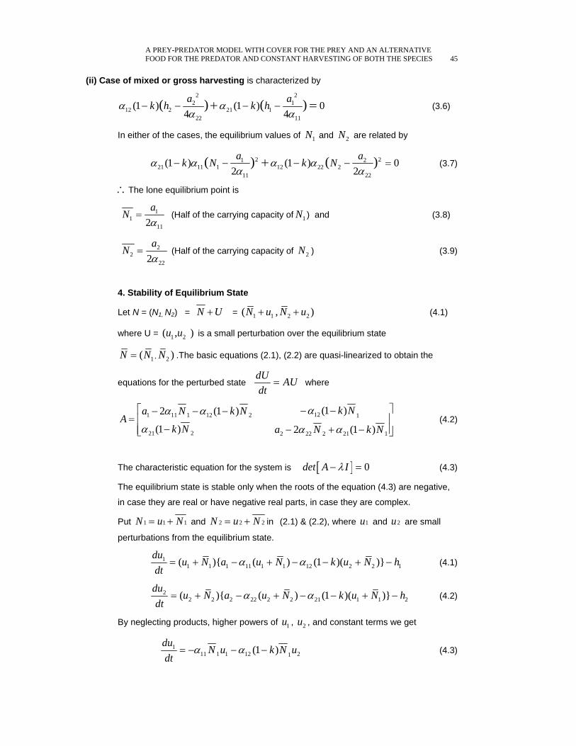
A PREY-PREDATOR MODEL WITH COVER FOR THE PREY AND AN ALTERNATIVE

FOOD FOR THE PREDATOR AND CONSTANT HARVESTING OF BOTH THE SPECIES 45

(ii) Case of mixed or gross harvesting is characterized by 2 2

2 112 2 21 1

22 11

(1 ) (1 ) 04 4

( ) ( )a ak h k hα α

α α− − − −+ = (3.6)

In either of the cases, the equilibrium values of 1N and 2N are related by

2 21 221 11 1 12 22 2

11 22

(1 ) (1 ) 02 2

( ) ( )a ak N k Nα α α α

α α− − − − =+ (3.7)

∴The lone equilibrium point is

11

112a

Nα

= (Half of the carrying capacity of 1N ) and (3.8)

22

222a

Nα

= (Half of the carrying capacity of 2N ) (3.9)

4. Stability of Equilibrium State

Let N = (N1, N2) = N U+ = 1 1 2 2( , )N u N u+ + (4.1)

where U = 1 2( , )u u is a small perturbation over the equilibrium state

,1 2( )N N N= .The basic equations (2.1), (2.2) are quasi-linearized to obtain the

equations for the perturbed state dU AUdt

= where

121 21 11 12 1

221 2 12 22 21

(1 )2 (1 )

(1 ) 2 (1 )

k Na N k NA

k N a N k N

αα α

α α α

⎤⎡ − −− − −= ⎥⎢

− − + − ⎥⎢⎣ ⎦ (4.2)

The characteristic equation for the system is [ ] 0det A Iλ− = (4.3)

The equilibrium state is stable only when the roots of the equation (4.3) are negative,

in case they are real or have negative real parts, in case they are complex.

Put 1 1 1N u N= + and 2 2 2N u N= + in (2.1) & (2.2), where 1u and 2u are small

perturbations from the equilibrium state.

11 1 1 11 1 1 12 2 2 1( ) ( ) (1 )( )

duu N a u N k u N h

dtα α= + − + − − + − (4.1)

22 2 2 22 2 2 21 1 1 2( ) ( ) (1 )( )

duu N a u N k u N h

dtα α= + − + − − + − (4.2)

By neglecting products, higher powers of 1u , 2u , and constant terms we get

1111 1 12 21(1 )

duN u k N u

dtα α= − − − (4.3)


and 2222 2 12 12 (1 )

duN u k u N

dtα α= − + − (4.4)

The characteristic equation is 2λ + 1 211 22( )N Nα α λ+ + 2

11 22 12 21[ (1 ) ]kα α α α+ − 1 2N N 0= (4.5)

The roots of which can be noted to be negative.

∴The co-existent equilibrium state is stable.

The trajectories are

1u = 2 110 1 22 20 12

1 2

( )- (1 )u N u N kλ α αλ λ

⎡ ⎤+ −⎢ ⎥−⎣ ⎦

1 teλ

+ 2 110 2 22 20 12

2 1

( )- (1 )u N u N kλ α αλ λ

⎡ ⎤+ −⎢ ⎥−⎣ ⎦

2 teλ (4.6)

2 =u 1 220 1 11 10 21

1 2

( )- (1 )u N u N kλ α αλ λ

⎡ ⎤+ −⎢ ⎥−⎣ ⎦

1 teλ +

1 220 2 11 10 21

2 1

( )- (1 )u N u N kλ α αλ λ

⎡ ⎤+ −⎢ ⎥−⎣ ⎦

2 teλ (4.7)

The curves are illustrated in Figures 1& 2. CASE 1: Initially the prey dominates the predator and it continues through out its

growth i.e. 10 20< u u . In this case the predator always outnumbers the prey. It is

evident that both the species are asymptotic to the equilibrium point. Hence this state

is stable.

CASE 2: The prey dominates the predator in natural growth rate but its initial strength

is less than that of predator. i.e. 10 20> u u . In this case, initially the prey outnumber the

predator and this continues the time instant t = t* given by equation (4.8), after which

the predator out number the prey.

= * =t t 2 1

1λ λ+

ln 3 5 10 3 1 20 2 6 10 4 1 20

( ) ( )( ) ( )

b a u a b ub a u a b u

⎡ ⎤⎢ ⎥⎢ ⎥⎢ ⎥⎣ ⎦

− + +− + +

(4.8)

where 3 1 11 1a Nλ α= + ; 4 2 11 1a Nλ α= + ; 25 1 22a Nλ α= + ;

26 2 22a Nλ α= + 11 12 (1 )b k Nα= − ; 22 21 (1 )b k Nα= − . (4.9)

As t →∞ both 1 2&u u approaches the equilibrium point. Hence the state is stable.



4.2. Trajectories of perturbed species

The trajectories in the 1 2-u u plane are given by

131 2 11 2

213

1 2 2

( - )( )( )

( )( - )1[ ]

( )p

p avu u va v vu d av

u v u

+ +−=

− (4.10)

where, 2 223p N α= (4.11)

and 1v , 2v are roots of quadratic equation 24+ + =0av bv c with

221= (1 )a N kα − ; 111 22 2=b N Nα α− ; 14 12= (1 )c N kα − (4.12)

and d , an arbitrary constant.

When 2 21 2 1 211 22 12 21( ) 4 (1 )N N k N Nα α α α− < − , (4.13)

the roots are complex with negative real part. Hence the equilibrium state is stable. The solution curves are illustrated in Figure .3.

When 2 21 2 1 211 22 12 21( ) 4 (1 )N N k N Nα α α α− > − , (4.14)

the roots are real and negative. Hence the equilibrium state is stable. The solution curves are illustrated in Figure .4.

5. Liapunov’s Function for Global Stability The Linearized Basic Equations for the model under investigation are

11 211 1 12 2(1 )

duN u k N u

dtαα= − − − (5.1)

22 221 1 22 2(1 )

duk N u N u

dtα α= − − − (5.2)

The characteristic equation is 2

1 2 1 211 22 12 21( )( ) (1 ) 0N N k N Nλ α λ α α α+ + + − = 2 0p qλ λ⇒ + + = (5.3)

where 1 211 22 0p N Nα α= + > and 21 211 22 12 21 (1 ) 0q k N Nα α α α= + − >

Hence the conditions for Liapunov’s function are satisfied.

Now we define 21 2 2 1 2 2

1( , ) ( 2 )2

E u u au bu u cu= + + (5.4)

where 2 2 2

2 1 221 22 2 11 22 12 21( (1 ) ) ( ) (1 ) k N N k N Na

Dα α α α α α− + + + −

= (5.5)


2 1 211 21 12 221(1 ) (1 )k N N k N Nb

Dα α α α−− −

= (5.6)

2 2 21 1 211 12 11 22 12 211( ) ( (1 ) ) (1 ) N k N k N N

c andD

α α α α α α+ − + + −= (5.7)

21 1 211 22 2 11 22 12 21 (1 ) D pq N N k N Nαα α α α α= = + + − (5.8)

From equations (5.5) & (5.8) it is clear that 0D > and 0a > . Also 2 2( )D ac b− =

2 2 2

2 2 1 221 22 2 11 22 12 21( (1 ) ) ( ) (1 ) k N N k N ND

Dα α α α α α− + + + −

× 2 2 2

1 1 211 12 11 22 12 211( ) ( (1 ) ) (1 ) N k N k N ND

α α α α α α+ − + + −−

2 2 2 2 2 22 2 2 2 2 2 21 2 1 2 1 211 21 12 22 11 12 21 22

2

(1 ) (1 ) 2 (1 )0k N N k N N k N N

Dα α α α α α α α− + − − −

>

(5.9)

Since 2 0D > , 2ac b− is also greater than zero. (5.10)

∴The function E(x, y) is positive definite.

Further,

1 2

1 2

du duE Eu dt u dt∂ ∂

+∂ ∂

= 1 11 2 11 1 12 2

21 2 21 1 22 22

( )[ (1 ) ]

( )[ (1 ) ]

au bu N u k N u

bu cu k N u N u

α α

α α

+ − − − +

+ − −

= 2 2

2 1 1 221 11 1 12 22 2

211 12 22 21 1 21

( (1 ) ) ( (1 ) )

[ (1 )] [ (1 )

b k N a N u b k N c N u

b a k N b c k N u u

α α α α

α α α α

−− − − + −

+ − + − − (5.11)

By substituting the values of a, b and c from equations (5.5),( 5.6) &(5.7) and

on simplification, we get

1 2

1 2

du duE Eu dt u dt∂ ∂

+∂ ∂

=

2 2 22 2 2 2

1 2 1 2 2 111 21 12 22 21 11 21[ (1 ) (1 ) (1 ) k N N k N N k N ND

α α α α α α α− −− − −−

2 2 22 2 22 2 211 22 11 22 12 11 21 21 1 1

1

(1 ) ]N N N N k N Nu

Dα α α α α α α− + −

−

2 2 22 2 2 2 22 2 212 11 21 12 22 11 221 1 1[ (1 ) (1 ) k N N k N N N N

Dα α α α α α α− − − +

+



2 2 22 2 22 2 1 2 112 22 11 22 12 22 21 21

2

(1 ) ]k N N N N N Nu

Dα α α α α α α− + +

−

2 2 22 2 2 2 32 2 2 111 21 12 11 22 12 211 1(1 ) (1 ) (1 ) k N N k N N k N N

Dα α α α α α α− − − + −

+

2 2 22 2 3

1 2 2 212 22 11 12 22 12 211 1(1 ) (1 ) (1 )k N N k N N k N ND

α α α α α α α− + − + −−

2 2 22 21 2 1 2 212 22 11 12 22 11 21 1(1 ) (1 ) (1 )k N N k N N k N N

Dα α α α α α α− + − − −

−

22 22 3 2 32 1 2 2 112 21 11 21 22 12 211

1 2

(1 ) (1 ) (1 ) k N N k N N k N Nu u

Dα α α α α α α− − − − −

=

2 21 2

D Du uD D

− −

⇒ 2 21 21 2

1 2

( )du duE E u u

u dt u dt∂ ∂

+ = − +∂ ∂

, (5.12)

which is clearly negative definite. So E(x, y) is a Lyapunov’s function for the linear

system.

Further we prove that E ( 1u , 2u ) is also a Lyapunov’s function for the non linear

system.

If, 1F and 2F are defined by

,1 1 2( )F N N = 1 1 11 1 12 2 1 (1 ) N a N k N hα α− − − − (5.13)

,2 1 2( )F N N = 2 2 22 2 21 1 2 (1 ) N a N k N hα α− − − − , (5.14)

we have to prove that 1 21 2

E EF Fu u∂ ∂

+∂ ∂

is negative definite.

By substituting 11 1N N u= + and 22 2N N u= + in (5.1) & (5.2) equations, we get

1dudt

= 1 1( )N u+ 1 21 11 11 1 12 12 2 (1 ) (1 ) a N u k N k uα α α α− − − − − − - 1h

From (5.13), ,1 1 2( )F u u = 1dudt

= 1 111 1 12 2(1 )N u k N uα α− − − + ,1 21 ( )u uf (5.15)

where ,1 21 ( )u uf = 211 1 12 1 2(1 )u k u uα α− − − - 1h (5.16)


Similarly ,2 1 2( )F u u = 2dudt

= 2 222 2 21 1(1 )N u k N uα α− − − + ,2 1 2( )u uf (5.17)

where ,2 1 2( )u uf = 222 2 21 1 2(1 )u k u uα α− + − - 2h (5.18)

And we have 1 21

E au buu∂

= +∂

and 1 22

E bu cuu∂

= +∂

(5.19)

By considering the equations (5.15),(5.17) and (5.19),

1 21 2

E EF Fu u∂ ∂

+∂ ∂

= 2 21 2( )u u− + ,1 2 1 21( ) ( )au bu u uf+ + ,1 2 2 1 2( ) ( )bu cu u uf+ + (5.20)

By introducing polar co-ordinates we get,

1 21 2

E EF Fu u∂ ∂

+∂ ∂

=

2, ,1 2 2 1 21[( cos sin ) ( cos sin ) ]( ) ( )r r a b u u b c u uf fθ θ θ θ− + + + + (5.21)

By denoting largest of the numbers , ,a b c by M,

our assumptions become ,1 21 ( )6

ru ufM

< and ,2 1 2( )6

ru ufM

< (5.22)

for all sufficiently small r 0> ,

so 1 21 2

E EF Fu u∂ ∂

+∂ ∂

2 22 4 0

6 3Kr rrM

< − + = − <

Thus E ( 1u , 2u ) is a positive definite function with the property that 1 21 2

E EF Fu u∂ ∂

+∂ ∂

is negative definite.

∴The equilibrium point is an asymptotically “stable”.

6. Threshold Theorem

In consonance with the principle of competitive exclusion [Gauss (1934)],

we deduce a Threshold Theorems for the lone equilibrium point.

The basic equations for the model under consideration can be re-written as

1 1 11 1 1 2 1

1

2 2 22 2 2 1 2

2

dN a Nk N N h

dt kdN a N

k N N hdt k

β

β

= − − −

= − − − (6.1)

where 11

11

ak

α= ; 2

222

ak

α= ; 12

11

(1 )ka

αβ

−= and 21

22

(1 )ka

αβ

−= − .



Theorem 1. Principle of Competitive Exclusion.

When 12

1

kk

β> and 2

12

kk

β> , then every solution of 1 2( ), ( )N t N t of (6.1) approaches

the equilibrium solution 11 ( )N t N= ( 0≠ ) and 22 ( )N t N= ( 0≠ ) as t approaches

infinity. In other words, if prey and predator species are nearly identical and the

microcosm can support both the members of prey and predator species depending up

on the initial conditions.

Proof: The first step in our proof is to show that 1 ( )N t and 2 ( )N t can never become

negative. To this end, observe that

111

11

( )2a

N t Nα

= = and 222

22

( )2a

N t Nα

= =

is a solution of (6.1) for any choice of 1 (0)N . The orbit of this solution in the

1 2N N− plane is the point (0, 0) for 1 (0) 0N = ; the line 1 10 N k< < , 2 0N =

for 1 10 (0)N k< < ; the point 1( ,0)k for 1 1(0)N k= ; and the line 1 1k N< < ∞ ,

2 0N = for 1 1(0)N k> . Thus the 1N axis, for 1 0N ≥ is the union of four distinct orbits

of (6.1). Similarly the 2N axis, for 2 0N ≥ , is the union of four distinct orbits of (6.1).

This implies that all solutions 1 2( ), ( )N t N t of (6.1) which start in the first quadrant

( )1 2( ) 0, 0N t N> > of the 1 2N N− plane must remain there for all future time.

The second step in our proof is to split the first quadrant into regions in which both

1dNdt

and 2dNdt

have fixed signs. This is accomplished in the following manner.

Let 1l and 2l be the lines 1 1 1 2 1k N N hβ− − = and 2 2 2 1 2k N N hβ− − = respectively

and the point of their intersection, is 1 2( , )N N . Observe that 1dNdt

is negative if

1 2( , )N N lies above the line 1l and positive if 1 2( , )N N lies below 1l . Similarly, 2dNdt

is negative if 1 2( , )N N lies above 2l and positive if 1 2( , )N N lies below 2l . Thus the

two lines 1l and 2l split the first quadrant of the 1 2N N− plane into four regions in

which both 1dNdt

and 2dNdt

have fixed signs.

1 2( ), ( )N t N t both increase with time in region I;

1 ( )N t increases and 2 ( )N t decreases with time in region II;


1 ( )N t decreases and 2 ( )N t increases with time in region III

and both 1 ( )N t and 2 ( )N t decrease with time in region IV. In this region both the

prey predator compete with each other but do not flourish and at the same time do not

get extinct.

Finally we require the following four lemmas.

Lemma 1. Any solution of 1 2( ), ( )N t N t of (6.1) which starts in region I at time 0t t=

will remain in this region for all future time 0t t≥ , and ultimately approach the

equilibrium solution 1 1( )N t N= , 2 2( )N t N= .(Figure 5)

Lemma 2. Any solution of 1 2( ), ( )N t N t of (6.1) which starts in region II at time 0t t=



Lemma 3. Any solution of 1 2( ), ( )N t N t of (6.1) which starts in region III at time 0t t=



Lemma 4. Any solution of 1 2( ), ( )N t N t of (6.1) which starts in region VI at time 0t t=



Lemmas 1, 2, 3 and 4 state that every solution 1 2( ), ( )N t N t of (6.1) which

starts in region I, II, III or VI at time 0t t= and remains there for all future time must

also approach equilibrium solution 11 ( )N t N= , 22 ( )N t N= as t approaches infinity.

Next, observe that any solution 1 2( ), ( )N t N t of (1) which starts on 1l or 2l must

immediately afterwards enter regions I, II, III or VI. Finally the solution approaches the

equilibrium solution 1 1( )N t N= , 2 2( )N t N= . This is illustrated in Figure 6



7. Trajectories

8. Future Work

In the present paper it is investigated that a Prey-Predator model with constant

harvesting of both species, a cover for prey and a limited alternate food is supplied to

the predator. There is a scope to study the model with constant harvesting of the prey

species, or constant harvesting of the predator species. Further cover can be removed

to the Prey and without an alternate food to the predator.


REFERENCES

[1] Michael Olinck, An introduction to Mathematical models in the social and Life

Sciences , Addison Wesley, 1978.

[2] Kapur, J. N., Mathematical models in Biology and Medicine, Affiliated East-

West,1985.

[3] Smith, J. M., Models in Ecology, Cambridge University Press, Cambridge, 1974.

[4] Paul Colinvaux, Ecology, John Wiley and Sons Inc., New York, 1977.

[5]. Freedman, H. I., Deterministic Mathematical Models in Population Ecology,

Marcel – Decker, New York, 1980.

[6] May, R. M., Stability and complexity in Model Eco-systems, Princeton University

Press, Princeton, 1973.

[7] Varma, V. S., A note on Exact solutions for a special prey-predator or competing

species system, Bull. Math. Biol., 39(1977), 619-622.

[8] Narayan, K. L., A Mathematical Study of Prey – Predator Ecological Models

with a Partial Cover for the Prey and Alternative Food for the Predator, Ph.D

thesis, JNTU, Hyderabad, 2005.

[9] Narayan, K.L. & Ramacharyulu,N.C.P, A Prey-Predator Model with an

Alternative Food for the Predator, harvesting of both the Species and with A

Gestation Period for Interaction, IJOPCM,1(1) ( 2008 ), 71-79.

[10] Narayan, K.L. & Ramacharyulu,N.C.P, A Prey-Predator Model with an

Alternative Food for the Predator, harvesting of both the Species and. A Time

Delay, Proceedings of ICM, UAE, ( 2008 ), 352-358.

[11] Narayan, K.L. & Ramacharyulu,N.C.P, A Prey-Predator Model with a cover

proportional to size of the Prey and an Alternative Food for the Predator, Int.

J. of Math. Sci. & Engg. Appls., 2(IV) (2008), 129-141.

[12] Narayan, K.L. & Ramacharyulu,N.C.P, “Some Threshold Theorems for a Prey-

Predator Model with Harvesting, Int.J. of Math. Sci. & Engg. Appls.,

2( II )(2008), 179-191 .

1Department of Mathematics & Humanities, SLC’S IET, Hyderabad-501 512, India.

2 Department of Mathematics & Humanities, NIT, Warangal-506 004, India.

E-mail address: [email protected]

للرياضيات واإلحصاء

املجلة األردنية

مجلة بحوث علمية عاملية محكمة

هـ1430 رجـــب/ م2009حزيــران ، )1(العدد ، )2(المجلد

محتويات العدد

Fractional Calculus Operators Associated with a Subclass of Uniformly Convex Functions G. Murugusundaramoorthy and R. Themangani

1

Some Properties of Unisrially Embedding of Subgroups of P-Groups Hassan Naraghi

11

Homotopy Analysis Method for Delay-Integro-Differential Equations Edris Rawashdeh, H. M. Jaradat and Fadi Awawdeh

15

An Alternative Proof of the Friendship Theorem Mohammad Bataineh

25

Some Applications of the Co-Hyponormal Operators Mohammad Rashid and Basem Masaedeh

33

A Prey-Predator Model with cover for the Prey and An Alternative Food for the Predator and Constant Harvesting of Both the Species K. Lakshimi Narayan and N. Pattabhiramacharyulu

43


جامعة اليرموك المملكة األردنية الهاشمية

ةاملجلة األردني

مجلة علمية عاملية محكمة

هـ1430 رجــــب / م2009 حزيــران ،)1( العدد ،)2(المجلد



مةعلمية عاملية محكبحوث مجلة

هـ1430 رجــب/ م2009 حزيــران، )1(العدد ، )2(المجلد ، التعليم العالي والبحث العلمي، األردنوزارةللبحث العلمي، أسستها اللجنة العليا مجلة علمية عالمية محكمة: للرياضيات واإلحصاءاملجلة األردنية

.وتصدر عن عمادة البحث العلمي والدراسات العليا، جامعة اليرموك، إربد، األردن

: التحريررئيس مشهور عبد الله الرفاعي .د.أ

قسم الرياضيات، جامعة اليرموك، اربد، األردن نائب رئيس جامعة اليرموك: الحاليالعنوان

E-mail: [email protected]

عمادة البحث العلمي والدراسات العليا ، منار ملكاوي السيدة :سكرتري التحرير

: هيئة التحرير نبيل طالب شواقفة. د.أ

م الرياضيات، الجامعة األردنية، عمان، األردنقس رئيس جامعة آل البيت، المفرق، األردن: العنوان الحالي


مفيد محمد عزام. د.أ قسم الرياضيات، الجامعة األردنية، عمان، األردن


أحمد ذيب عالونة. د.أ معة األردنية، عمان، األردنقسم الرياضيات، الجا


بسام يوسف الناشف. د.أ ، األردنإربدجامعة اليرموك، قسم الرياضيات،


فؤاد أسعد كتانة. د.أ قسم الرياضيات، الجامعة األردنية، عمان، األردن


د الجراحعبد الله محم. د.أ ، األردنإربدقسم الرياضيات، جامعة اليرموك، E-mail: [email protected]

.قسم الرياضيات، جامعة اليرموك، الجراح محمدعبد الله. د.أ : العلمياملحرر

-: البحوث إلى العنوان التالي ترسل األستاذ الدكتور مشهور عبد الله الرفاعي

جلة األردنية للرياضيات واإلحصاء المررئيس تحري األردن- إربد، ة البحث العلمي والدراسات العليا، جامعة اليرموكعماد

2026 فرعي 00 962 2 7211111 هاتفE-mail: [email protected]

Website: http://jjms.yu.edu.jo


جامعة اليرموك المملكة األردنية الهاشمية


مجلة علمية عاملية محكمة

هـ1430 رجــب / م2009 حزيــــران ،)1( العدد ،)2(المجلد

Jordan Journal of Mathematics and Statistics - …journals.yu.edu.jo/jjms/Issues/vol2No12009/JJMS...

Documents

Transcript of Jordan Journal of Mathematics and Statistics - …journals.yu.edu.jo/jjms/Issues/vol2No12009/JJMS...