
Joint Sparsity for Target Detection - The Norbert Wiener ... M. Nasrabadi Joint Sparsity for Target...
24
UNCLASSIFIED Nasser M. Nasrabadi Joint Sparsity for Target Detection Nasser M. Nasrabadi UNCLASSIFIED U.S. Army Research Laboratory
Transcript of Joint Sparsity for Target Detection - The Norbert Wiener ... M. Nasrabadi Joint Sparsity for Target...

UNCLASSIFIED
Nasser M. NasrabadiJoint Sparsity for Target Detection
Nasser M. Nasrabadi
UNCLASSIFIED
U.S. Army Research Laboratory

Introduction
• Objective: Segmentation of HSI into multiple classes (target and background) or classifyclasses (target and background) or classify individual objects (military targets) from multiple views of the same physical target.
• Assumptions– Training data: known spectral characteristics (or
images) of different classesimages) of different classes– Test data: a sparse linear combination of all
training data– In HSI Neighboring pixels: similar materials– Mutiple views of targets are similar
• Results compared to classical SVM classifiers

Hyperspectral Imagery

Pixel-wise Sparsity Model
• Background pixels approximately lie in a low-di i l bdimensional subspace
,1 1 ,2 2 , b b
b b b b b b b bi i i i N N i a a Aa αx
• Target pixels also lie in a low-dimensional subspace
t t t t t tt tA• A test sample can be sparsely represented
b
,1 1 ,2 2 , t t
t t t ti i i i N
t ti
tN
t a a a αx A
ixby
bb b t t b t i
i i i it
A A A A Ax
i i i it
i

Ilustration: Pixel-Wise Sparse Model
0 . 1 2
0 . 1 4
0 . 0 6
0 . 0 7
0 . 0 8
0 . 0 9
0 . 1
0 . 1 1t e s t s a m p l e
0 . 0 6
0 . 0 8
0 . 1
b a c k g ro u n d d ic t io n a ry
0 5 0 1 0 0 1 5 0
0 . 0 4
0 . 0 5
0 5 0 1 0 0 1 5 00 . 0 2
0 . 0 4
t a rg e t d ic t io n a ry
Target Pixel
b
Test Spectrum ix Nonzero entries
Spectral dictionary A
bb b t t b t i
i i i iti
A A A A Ax

Sparse Recovery
• Sparse coefficient is recovered by
ˆ arg min subject to A x
• For empirical data0
arg min subject toi i i i A x
0 2ˆ arg min subject to
ˆ arg min subject toi i i i
K
A x
A x
• NP-hard problemGreedy algorithms: MP OMP SP C S MP LARS
02 0arg min subject toi i i i K A x
– Greedy algorithms: MP, OMP, SP, CoSaMP, LARS
– Convex relaxation: Iterative Thresholding, Primal-Dual Interior-Point, Gradient Projection, Proximal Gradient, Augmented Lagrange Multiplier
1ˆ arg min subject toi i i i A x

Classification Based on Residuals
• Recover sparse coefficientˆ
ˆbi
i
Recover sparse coefficient
• Compute the residuals (approximation errors
ˆi ti
Compute the residuals (approximation errors w.r.t. the two sub-dictionaries)
ˆ ˆb b t t 2 2
and ˆ ˆ b bi i i i
tb t i i
tr r x A x Ax x
• Class of test pixel is made by comparing the residuals
ix

Example: Reconstruction
0 . 6
0 . 7
0 . 8
0 . 9R e c o v e r e d s p a r s e c o e f f i c i e n t s
ˆ b
0 2
0 . 3
0 . 4
0 . 5ˆˆ
bi
i ti
0 5 0 1 0 0 1 5 0 2 0 0 2 5 00
0 . 1
0 . 2
0 . 1 2
0 . 0 8
0 . 1
ˆ ˆt t t Ax
0 . 0 2
0 . 0 4
0 . 0 6
O r i g i n a lR e c o n s t r u c t e d fr o m b g d i c .
i iAx
ˆ ˆib
ib b Ax
0 5 0 1 0 0 1 5 00
0 0
e c o s t u c t e d o b g d cR e c o n s t r u c t e d fr o m t a r g e t

Joint Sparsity Model(Joint Structural Sparsity Prior)
• Use of contextual information– Neighboring pixels: similar spectral characteristicsg g p p– Approximated by the same few training samples, weighed
differently• Consider T pixels in a small neighborhood• Consider T pixels in a small neighborhood
1 1 AA
x
2 2 Ax
1 2 1 2T T S
X x x x A AS
– ’s: sparse vectors with same support, different magnitude
T T Ax
i p pp , g– : sparse matrix with only a few nonzero rows
i
S

Illustration: T=3x3 Neighborhood
0.140.14
9
0.1
0.12
0.08
0.1
0.12
0 04
0.06
0.08
0.04
0.06 T=9
0 50 100 1500.02
0.04
0 50 100 1500
0.02
X Spectral dictionary A Row-sparse t i S
Data matrixmatrix S

Joint Sparse Recovery
• is recovered byS
• Solved by greedy algorithms: Simultaneous OMProw, 0
ˆ arg min subject to S S AS X
• Solved by greedy algorithms: Simultaneous OMP (SOMP) , Simultaneous SP (SSP) or Convex optimization to find the same active set
1,2ˆ arg min subject to S S AS X
• Decision obtained by comparing total residuals

Comparison of single pixel sparsity model VS Joint Sparsity Recovery
Model (k=5 atoms active)
Input a singleInput a single background pixel x
0ˆ arg min subject to A x
Input nine put e
neighboringbackground pixels X
row, 0ˆ arg min subject to S S AS X

Results on HYDICE FR-I
Original image (averaged Proposed detector outputg g ( gover 150 bands)
p p

Results on FR-I: ROC Curves

Extension to Multiple Classes
• AVIRIS HSI data set with 16 classes, 220 bands, 20 meters pixel resolution220 bands, 20 meters pixel resolution

Extension to Multiple Classes
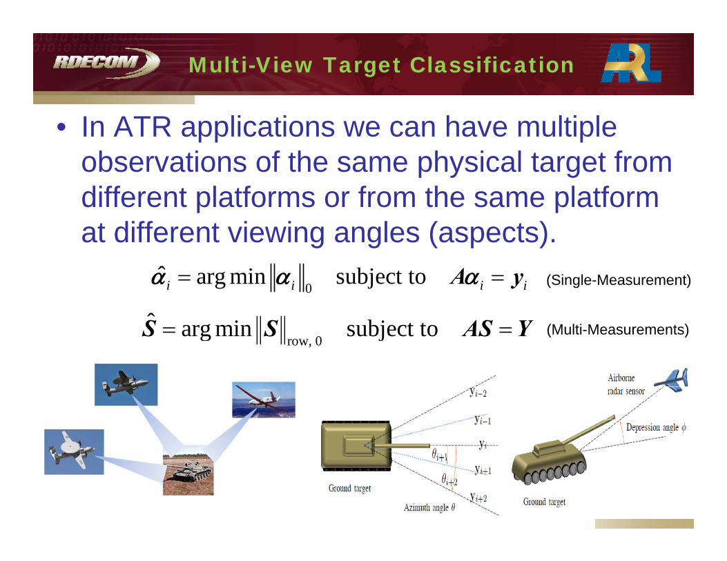
Multi-View Target Classification
• In ATR applications we can have multiple observations of the same physical target from p y gdifferent platforms or from the same platform at different viewing angles (aspects).g g ( p )
0ˆ arg min subject toi i i i A y
ˆ
(Single-Measurement)
row, 0ˆ arg min subject to S S AS Y (Multi-Measurements)

Experimental Results on Multi-View Target Classification
• MSTAR SAR data-base consists of 10 militaryconsists of 10 military targets at roughly 1-3 interval azimuth angles (0-360 ) t t diff t
360 ) at two different depression angles 15 and 17 . Data from 17 is used for
training (dictionary design) 15 is used for testing

Experimental Results on Multi-View Target Classification
• Three class (BMP2, BTR70, T72) target classification C=3 with multiple views M=3 . Features are incoherent random projections dimension range from d=128 to1024.
0ˆ arg min subject toi i i i A x
1 1
0ˆ arg min subject to
and
A x
xA x
row, 0
1
ˆ arg min subject to
Note [ ]M
S S AS X
S
M M x

Experimental Results on Number of Views and Angle Size
• Effect of different number of views M
• Effect of the angle size between the views

Experimental Results on Multi-View Target Classification
• 10 class classification results using M=3 views with dictionary of size yN=2747 tested on 15 degree depression g p

Multi-Pose Face Recognition
• Scenarios where we have multiple poses of the same face as input to the classifier.
• UMIST database consists of 564 images of 20 individuals with a range of poses.
• Randomly select 10 poses for each individual to construct the dictionary.

Conclusions
• Formulated target and object recognition as joint sparsity underdetermined regression problem.
• Investigated the effect single vs multiple measurements • Included the idea of joint structured sparsity prior into
th l i ti t f th ti i tithe regularization part of the optimization• Investigated performance of multiple measurements on
classification performance on several data bases. p

Thank You
THANK YOU