Federal Reserve Bank of Minneapolis

Research Department Staff Report 426

May 2009

Joint-Search Theory:New Opportunities and New Frictions∗

Bulent Guler

University of Texas at Austin

Fatih Guvenen

University of Minnesota,

Federal Reserve Bank of Minneapolis,

and NBER

Giovanni L. Violante

New York University,

CPER,

and NBER

ABSTRACT

Search theory routinely assumes that decisions about the acceptance/rejection of job offers (and,

hence, about labor market movements between jobs or across employment states) are made by

individuals acting in isolation. In reality, the vast majority of workers are somewhat tied to their

partners–in couples and families–and decisions are made jointly. This paper studies, from a

theoretical viewpoint, the joint job-search and location problem of a household formed by a couple

(e.g., husband and wife) who perfectly pools income. The objective of the exercise, very much in the

spirit of standard search theory, is to characterize the reservation wage behavior of the couple and

compare it to the single-agent search model in order to understand the ramifications of partnerships

for individual labor market outcomes and wage dynamics. We focus on two main cases. First, when

couples are risk averse and pool income, joint search yields new opportunities–similar to on-the-job

search–relative to the single-agent search. Second, when the two spouses in a couple face job offers

from multiple locations and a cost of living apart, joint search features new frictions and can lead

to significantly worse outcomes than single-agent search.

∗Guler: bguler@mail.utexas.edu. Guvenen: guvenen@umn.edu. Violante: gianluca.violante@nyu.edu. Theviews expressed herein are those of the authors and not necessarily those of the Federal Reserve Bank of

Minneapolis or the Federal Reserve System.

1 Introduction

In the year 2000, over 60% of the US population was married, the labor force participation rate ofmarried women stood at 61%, and in one-third of married couples wives provided more than 40% ofhousehold income (US Census (2000); Raley, Mattingly, and Bianchi (2006)). For these households,which make up a substantial fraction of the population, economic decisions are jointly taken by thetwo spouses. Among such decisions, job search, broadly defined, is arguably one of the most crucialto the economic well-being of a household.

Macroeconomics is rapidly shifting away from the stylized “bachelor model” of the household byexplicitly recognizing the relevance of household-level decisions for aggregate economic outcomes.1

Surprisingly, instead, since its inception in the early 1970s, search theory has almost entirely fo-cused on the single-agent search problem. The recent survey by Rogerson, Shimer, and Wright(2005), for example, does not contain any discussion on optimal job search strategies of two-personhouseholds acting as the decision units. This state of affairs is rather surprising given that Burdettand Mortensen (1977), in their seminal piece entitled “Labor Supply Under Uncertainty,” lay out atwo-person search model and sketch a characterization of its solution, explicitly encouraging furtherwork on the topic. Their pioneering effort, which remained virtually unfollowed, represents thestarting point of our theoretical analysis.

In this paper, we study the job search problem of a couple who faces exactly the same economicenvironment as in the standard single-agent search problem of McCall (1970) and Mortensen (1970)without on-the-job search, and Burdett (1978) with on-the-job search. A couple is an economicunit composed of two identical individuals linked to each other by the assumption of perfect incomepooling. The simple unitary model of a household adopted here is a convenient and logical startingpoint. It helps us to examine more transparently the role of the labor market frictions and insuranceopportunities introduced by joint-search, and it makes the comparison with the canonical single-agent search model especially stark.

From a theoretical perspective, couples would make a joint decision leading to choices differentfrom those of a single agent for several reasons. We start from the two most natural and relevantones. First, the couple has concave preferences over pooled income. Second, the couple can receivejob offers from multiple locations, but faces a utility cost of living apart. In this latter, casedeviations from the single-agent search problem occur even for linear preferences. As summarizedby the title of our paper, in the first environment joint search introduces new opportunities, whereasin the second it introduces new frictions relative to single-agent search. One appealing feature ofour theoretical analysis is that it leads to two-dimensional diagrams in the space of the two spouses’wages (w1, w2), where the reservation wage policies can be easily analyzed and interpreted.

In the first environment we study, couples have risk-averse preferences and have access to a1For example, see Aiyagari et al. (2000) on intergenerational mobility and investment in children, Cubeddu and

Rios-Rull (2003) on precautionary saving, Blundell et al. (2007) on labor supply, Heathcote et al. (2008) and Liseand Seitz (2008) on economic inequality, and Guner et al. (2009) on taxation.

2

risk-free asset for saving but are not allowed to borrow. A dual-searcher couple (both membersunemployed) will quickly accept a job offer—in fact, more easily than a single unemployed agent.However, the worker-searcher couple (one spouse unemployed, the other employed) will be morechoosy in accepting the second job offer. The dual-searcher couple can use income pooling to itsadvantage: it initially accepts a lower wage offer (to smooth consumption across states) while, atthe same time, not giving up completely the search option (to increase lifetime income) that remainsavailable to the other spouse. We formally show that the gap between the reservation wage of theworker-searcher couple (a function of the employed spouse’s wage) and that of the dual-searchercouple (a constant) depends on the degree of absolute risk aversion in preferences, and on howabsolute risk aversion changes with the level of consumption.

Furthermore, if the second spouse receives and accepts a very good job offer, this may trigger aquit by the employed spouse to search for a better job, resulting in a switch between the breadwinnerand the searcher within the household. As is well known, this endogenous quit behavior neverhappens in the standard single-agent version of the search model. We call this process—of quit-search-work that allows a couple to climb the wage ladder even in absence of on-the-job search—the“breadwinner cycle.” Therefore, one can view joint search as a “costly” version of on-the-job search,even in the formal absence of it. The cost comes from the fact that in order to keep the searchoption active, the pair must remain a worker-searcher couple, and must not enjoy the full wageearnings of a dual-worker couple as it would be capable of doing in the presence of on-the-jobsearch. Overall, relative to singles, couples spend more time searching for better jobs, which resultsin longer unemployment durations, but it eventually leads to higher lifetime wages and welfare.

We uncover two “equivalence results” between single-agent search and joint-search outcomes.The first environment requires the presence of on-the-job search, with equal search effectivenesson and off the job. The second requires the presence of loose borrowing limits. In both cases,a risk-averse couple acts like a single agent. These equivalence results follow directly from thevalue added of joint search in terms of climbing the wage ladder and of smoothing consumption,as discussed above. Finally, we also show an intuitive and useful result: the joint-search model isexactly isomorphic to a model where a single agent searches for jobs, and she has the possibility ofholding multiple jobs.

Our second model features two locations and a flow cost of living apart for the two spousesin the couple. The couple has to choose reservation functions with respect to “inside offers” (jobsin the current location) and “outside offers” (jobs in the other location). Even with risk-neutralpreferences, the search behavior of couples differs from that of single agents in important ways.First, the dual-searcher couple is less choosy than the individual agent because it is effectivelyfacing a worse job offer distribution, since some wage offer configurations are attainable only indifferent locations—hence, by paying the cost of living apart. Second, there is a region in which thebreadwinner cycle is optimal for the couple. For example, a couple who keeps getting better andbetter offers from the outside location could be better off if the currently employed spouse quitsand follows the spouse with the highest offer to the new location. It should be noted that we also

3

obtained these two results in our previous environment, but for completely different reasons.The model allows us to formalize what Mincer (1978) called tied-stayers—i.e., workers who turn

down a job offer in a different location that they would accept as single—and tied-movers—i.e.,workers who accept a job offer in the location of the partner that they would turn down as single.Overall, the disutility of living separately effectively narrows down the job offers that are viablefor couples, who end up choosing among a more limited set of job options. We show, throughsimulations, that for plausible parameter values, joint search yields outcomes that are significantlydifferent from single-agent search. For example, when the disutility cost (of living separately) is equalto 15% of a dual-worker couples’ average wage earnings, more than half of all moving householdsinvolve a partner who is a tied-mover, and the lifetime income of each spouse in a couple is 6.5%lower than comparable singles.

The set of propositions proved in the paper formalizes the new opportunities and the new frictionsin terms of comparison between the reservation wage functions of the couple and the reservationwage of the single agent. We also provide some illustrative simulations to show that the deviationsof joint-search behavior from its single-agent counterpart can be quantitatively substantial.

Only very recently, a handful of papers have started to follow the lead offered by Burdett andMortensen (1977) into the investigation of household interactions in frictional labor market models.Garcia-Perez and Rendon (2004) numerically simulate a model of family-based job-search decisionsto tease out the importance of the added worker effect for consumption smoothing. Dey and Flinn(2008) study quantitatively the effects of health insurance coverage on employment dynamics in asearch model where the economic unit is the household. Gemici (2008) estimates a rich structuralmodel of migration and labor market decisions of couples to assess the implications of joint locationconstraints on labor outcomes and the marital stability of couples. Relative to these contributions,our paper is less ambitious in its quantitative analysis, but it provides a more focused and systematicstudy of joint-search theory.

From a theoretical perspective, our analysis of the one-location model has useful points of con-tacts with existing results in search theory applied to at least three separate contexts. First, startingfrom the static analysis of Danforth (1979), a number of papers have studied the role of risk-freewealth in shaping dynamic job-search decisions (e.g., Browning et al., 2003; Pissarides, 2004; Lentzand Tranaes, 2005). The income of the spouse differs crucially from risk-free wealth because it isrisky (in the presence of exogenous separations), and because it can be optimally controlled by thejob-search decision itself. Second, Albrecht and Vroman (2009) study a different type of joint-searchdecision, that of a committee that votes on an option which gives some value to each member. Theauthors are interested in drawing a comparison between single-agent search and committee search,in the same spirit as our exercise.2 Third, as we explain in the main text, there is an analogy with

2The similarities, though, stop here more or less. For example, Albrecht and Vroman (2009) also find thatcommittees are less picky than single agents. In our one-location model, this result is due to a consumption-smoothingargument. In their environment, it is due to the negative externality that committee members impose on each other(e.g., voting against when drawing a particularly low value).

4

some search models of marriage formation where the flow value of the marriage is a concave functionof the sum of the spouses’ endowments (e.g., Visschers, 2006).

The rest of the paper is organized as follows. Section 2 describes the single-agent problemwhich provides the benchmark of comparison throughout the paper. Section 3 develops and fullycharacterizes the baseline joint-search problem. Section 4 extends this baseline model in a numberof directions: nonparticipation, on-the-job search, exogenous separations, and access to borrowing.Section 5 studies an economy with multiple locations and a cost of living apart for the couple.Section 6 concludes the paper and discusses how to relax some of the stark assumptions we made.The Appendix contains detailed proofs of all our propositions.

2 The Single-Agent Search Problem

We begin by first presenting the sequential job-search problem of a single agent—the well-knownMcCall-Mortensen model (McCall, 1970; Mortensen, 1970). This model provides a useful benchmarkagainst which we compare the joint-search model, which we introduce in the next section. Forclarity of exposition, we begin with a very stylized version of this optimal stopping problem, andthen consider several extensions in Section 4.

Economic environment. Consider an economy populated with individuals who all participatein the labor force: agents are either employed or unemployed. Time is continuous and there is noaggregate uncertainty. Workers maximize the expected lifetime utility from consumption,

E0

∫ ∞0

e−rtu (c (t)) dt,

where r is the subjective rate of time preference, c (t) is the instantaneous consumption flow at timet, and u (·) is the instantaneous utility function.

An unemployed worker is entitled to an instantaneous benefit, b, and receives wage offers, w, atrate α from an exogenous wage offer distribution, F (w) with support [0,∞). The worker observesthe wage offer, w, and decides whether to accept or reject it. If he accepts the offer, he becomesemployed at wage w forever. If he rejects the offer, he continues to be unemployed and to receive joboffers. All individuals are identical in terms of their labor market prospects, i.e., they face the samewage offer distribution and the same arrival rate of offers, α. There are no exogenous separationsand no on-the-job search. Finally, we assume that individuals have access to risk-free saving but arenot allowed to borrow. As will become clear below, in the present framework individuals face a wageearnings profile that is nondecreasing over the life cycle (without exogenous separation risk), and,therefore, consumption smoothing only requires the ability to borrow but does not benefit from theability to save. As a result, individuals will optimally set consumption equal to their wage earningsevery period even though they are allowed to save.3

3Borrowing, on-the-job search, exogenous job separation, and nonparticipation are introduced in Section 4.

5

Value functions. Denote by V and W the value functions of an unemployed and employedagent, respectively. Then, using the continuous time Bellman equations, the problem of a singleworker can be written in the following flow value representation:4

rV = u (b) + α

∫max W (w)− V, 0 dF (w) , (1)

rW (w) = u (w) . (2)

This well-known problem yields a unique reservation wage, w∗, for the unemployed such thatfor any wage offer above w∗, she accepts the offer and below w∗, she rejects the offer. Furthermore,this reservation wage can be obtained as the solution to the following equation:

u (w∗) = u (b) +α

r

∫w∗

[u (w)− u (w∗)] dF (w) (3)

= u (b) +α

r

∫w∗u′ (w) [1− F (w)] dw,

which equates the instantaneous utility of accepting a job offer paying the reservation wage (left-hand side, LHS) to the option flow value of continuing to search in the hope of obtaining a betteroffer in the future (right-hand side, RHS). Since the LHS is increasing in w∗, whereas the RHS is adecreasing function of w∗, equation (3) uniquely determines the reservation wage, w∗.

3 The Joint-Search Problem

We now study the search problem of a couple facing the same economic environment describedabove. For the purposes of this paper, a “couple” is defined as an economic unit composed of twoindividuals who are ex ante identical in their preferences and the labor market parameters they face.The two individuals perfectly pool income to purchase a market good which is jointly consumed bythe couple.

As before, because households are not able to borrow and saving is not optimal, they simplyconsume their total income in each period, which is the sum of the wage or benefit income of eachspouse. Couples make their job acceptance/rejection/quit decisions jointly, because each spouse’ssearch behavior affects the couple’s joint welfare.

A couple can be in one of three labor market states. First, if both spouses are unemployed andsearching, they are referred to as a “dual-searcher couple.” Second, if both spouses are employed(an absorbing state), we refer to them as a “dual-worker couple.” Finally, if one spouse is employedand the other is unemployed, we refer to them as a “worker-searcher couple.” As can perhaps beanticipated, the most interesting state is the last one.

4Below, when the limits of integration are not explicitly specified, they are understood to be the lower and upperbound of the support of w.

6

Value functions. Let U denote the value function of a dual-searcher couple, Ω (w1) the valuefunction of a worker-searcher couple when the worker’s wage is w1, and T (w1, w2) the value functionof a dual-worker couple earning wages w1 and w2. The flow value in the three states becomes

rT (w1, w2) = u (w1 + w2) , (4)

rU = u (2b) + 2α∫

max Ω (w)− U, 0 dF (w) , (5)

rΩ (w1) = u (w1 + b) + α

∫max T (w1, w2)− Ω (w1) ,Ω (w2)− Ω (w1) , 0 dF (w2) . (6)

The equations determining the first two value functions (4) and (5) are straightforward analogsof their counterparts in the single-search problem. In the first case, both spouses stay employedforever, and the flow value is simply equal to the total instantaneous wage earnings of the household.In the second case, the flow value is equal to the instantaneous utility of consumption (which equalsthe total unemployment benefit) plus the expected gain in case a wage offer is received. Becauseboth agents receive wage offers at rate α, the total offer arrival rate of a dual-searcher couple is 2α.5

Once a wage offer is received by either spouse, it will be accepted if it results in a gain in lifetimeutility (i.e., Ω (w)− U > 0), otherwise it will be rejected.

The value function of a worker-searcher couple is somewhat more involved. As can be seen inequation (6), if a couple receives a wage offer (which now arrives at rate α, since only one spouse isunemployed), three choices now face the couple. First, the unemployed spouse can reject the offer,in which case there is no change in the value. Second, the unemployed spouse can accept the joboffer and both spouses become employed, which increases the value by T (w1, w2)−Ω (w1) . Third,and finally, the unemployed spouse can accept the job offer and the employed spouse simultaneouslyquits his job and starts searching for a better one.

As we shall see below, this third case is the first important difference between the joint-searchproblem and the single-agent search problem. In the single-search problem, once an agent acceptsa job offer, she will never choose to quit her job. This is because an agent strictly prefers beingemployed to searching at any wage offer higher than the reservation wage. Because the environmentis stationary, the agent will face the same wage offer distribution upon quitting and will have thesame reservation wage. As a result, a single employed agent will never quit, even if he is given theopportunity. In contrast, in the joint-search problem, the reservation wage of each spouse dependson the income of the partner. When this income grows—for example, because of a transition fromunemployment to employment—the reservation wage of the previously employed spouse may alsoincrease, which could lead to exercising the quit option. We return to this point below and discussit in more detail.

5Because time is continuous, the probability of both spouses receiving offers simultaneously is negligible and ishence ignored.

7

3.1 Characterizing the couple’s decisions

Before we begin characterizing the solution to the problem, we state the following useful lemma.We refer to Appendix A for all the proofs and derivations.

Lemma 1 Ω is a strictly increasing function, i.e., Ω′(w) > 0 for all w ∈ [0,∞).

We are now ready to characterize the couple’s search behavior. First, for a dual-searcher couple,the reservation wage—which is the same for both spouses by symmetry—is denoted by w∗∗ and isdetermined by the equation

Ω (w∗∗) = U. (7)

Because U is a constant and Ω is a strictly increasing function (Lemma 1), w∗∗ is a singleton.A worker-searcher couple has two decisions to make. The first decision is whether to accept

the job offer to the unemployed spouse (say, spouse 2) or not. The second decision, conditional onaccepting, is whether the employed spouse (spouse 1) should quit his job or not. Let the currentwage of the employed spouse be w1 and denote the wage offer to the unemployed spouse by w2.6

Accept/reject decision. Let us begin by supposing that it is not optimal to exercise the quitoption upon acceptance, T (w1, w2) > Ω (w2). In this case, a job offer with wage w2 will be acceptedwhen T (w1, w2) ≥ Ω (w1) . Formally, the associated reservation wage function φ (w1) solves

T (w1, φ (w1)) = Ω (w1) . (8)

Suppose now instead that it is optimal to exercise the quit option upon acceptance, Ω (w2) ≥T (w1, w2). Then, the job offer will be accepted when Ω (w2) ≥ Ω (w1), which implies the reservationrule

Ω (φ (w1)) = Ω (w1) . (9)

Given the strict monotonicity of Ω, the reservation wage rule is very simple: accept the new offer(and the other spouse will quit the existing job) whenever w2 ≥ w1. The worker-searcher reservationwage function φ (·) is therefore piecewise, being composed of (8) and (9) in different ranges of thedomain for w1. The kink of this piecewise function, which always lies on the 45 degree line of the(w1, w2) space, plays a special role in characterizing the behavior of the couple. We denote this pointby (w, w), and formally it satisfies: T (w, φ (w)) = Ω (w) = Ω (φ (w)).7 Since rT (w, w) = u (2w), wsolves

u (2w) = Ω (w) . (10)6To better understand the optimal choices of the couple, it is instructive to treat the accept/reject decision of

the unemployed spouse and the stay/quit decision of the employed spouse as two separate choices (albeit the couplemakes them simultaneously).

7Given some further assumptions about the preferences, it will be clear that w is unique.

8

Stay/quit decision. It remains to characterize the quitting decision. If T (w1, w2) ≤ Ω (w2) ,it is optimal for the employed spouse to quit his job when the unemployed spouse accepts her joboffer (that is, this choice yields higher utility than would be the case if he stayed at his job and thecouple became a dual-worker couple). This inequality implies the indifference condition:

T (w1, ϕ (w1)) = Ω (ϕ (w1)) . (11)

Two important properties of ϕ should be noted. First, ϕ is not necessarily a function; it may be acorrespondence. Second, ϕ is the inverse of that piece of the φ function defined by (8). This is easilyseen. By symmetry of T , from (8) we have that T (φ (w1) , w1) = Ω (w1), or T

(w2, φ

−1 (w2))

=Ω(φ−1 (w2)

), which compared to (11) yields the desired result.

Since ϕ = φ−1, then ϕ will also cross the function φ on the 45-degree line at the point w. There-fore, w is the highest wage level at which the unemployed spouse is indifferent between acceptingand rejecting her offer and the employed partner is indifferent between keeping and quitting his job.To emphasize this feature, we refer to w as the “double indifference point.”

In what follows, we characterize the optimal strategy of the couple in the (w1, w2) space. Thismeans establishing the ranking between w∗∗ and w, especially in relation to the single-agent reser-vation wage w∗ and studying the function φ. Once we have characterized the shape of φ, that ofφ−1 follows immediately. Overall, these different reservation rules will divide the (w1, w2) into fourregions: one in which both spouses work, one where both spouses search, and the remaining tworegions in which spouse 1 (2) searches and spouse 2 (1) works.

3.2 Risk neutrality

As will become clear below, risk aversion is central to our analysis. To provide a benchmark, webegin by presenting the risk-neutral case, then turn to the results with risk-averse agents.

Proposition 1 [Risk neutrality] With risk-neutral preferences, i.e., u′′ = 0, the joint-searchproblem reduces to two independent single-search problems. Specifically, the value functions are

T (w1, w2) = W (w1) +W (w2) ,

U = 2V,

Ω (w1) = V +W (w1) .

The reservation wage function φ (·) of the worker-searcher couple is constant and is equal to thereservation wage value of a dual-searcher couple (regardless of the wage of the employed spouse),which, in turn, equals the reservation value in the single-search problem, i.e., φ (w1) = w∗∗ = w∗.

Figure 1 shows the relevant reservation wage functions in the (w1, w2) space, where w1 and w2

are the wages of spouses 1 and 2, respectively. In this paper, when we discuss worker-searchercouples, we will think of spouse 1 as the employed spouse and display his wage w1 on the horizontal

9

Figure 1: Reservation Wage Functions with Risk Neutrality

axis, and think of spouse 2 as the unemployed spouse and display her wage offer (w2) on the verticalaxis.

As stated in the proposition, the reservation wage function of a worker-searcher couple, φ (w1) issimply the horizontal line at w∗∗. Similarly, the reservation wage for the quit decision is the inverse(mirror image with respect to the 45-degree line) of φ (w1) and is shown by the vertical line atw1 = w∗∗. The intersection of these two lines gives rise to four regions, in which the couple displaysdistinct behaviors.

No wage below w∗∗ is ever accepted by a dual-searcher couple in this model. Therefore, aworker-searcher couple will never be observed with a wage below w∗∗. As a result, the only wagevalues relevant for the employed spouse are above the φ (w1) function. If the unemployed spousereceives a wage offer w2 < w∗∗, she rejects the offer and continues to search. If she receives an offerhigher than w∗∗, she accepts the offer. At this point the employed partner retains his job, and thecouple becomes a dual-worker couple.

For things to get interesting, risk aversion must be brought to the fore. In Section 5, we willalso see that when the job-search process takes place in multiple locations and there is a cost ofliving separately for the couple, then even in the risk-neutral case there are important deviationsfrom the single-agent search problem.

3.3 Risk aversion

To introduce risk aversion into the present framework, we employ preferences in the HARA (hyper-bolic absolute risk aversion) class. This class encompasses several well-known utility functions asspecial cases. Formally, HARA preferences are defined as the family of utility functions that have

10

linear risk tolerance: −u′ (c) /u′′ (c) = a+ τc, where a and τ are parameters.8

This class can be further divided into three subclasses depending on the sign of τ . First,when τ ≡ 0, then risk tolerance (and hence absolute risk aversion) is independent of consumptionlevel. This case corresponds to constant absolute risk aversion (CARA) preferences, also known asexponential utility u (c) = −e−ac/a. Second, if τ > 0 then absolute risk tolerance is increasing—and therefore risk aversion is decreasing—with consumption, which is the decreasing absolute riskaversion (DARA) case. A well-known special case of this class is the constant relative risk aversion(CRRA) utility: u (c) = c1−ρ/ (1− ρ) , which obtains when a ≡ 0 and τ = 1/ρ > 0. Finally, if τ < 0risk aversion increases with consumption, and this class is referred to as increasing absolute riskaversion (IARA). A special case of this class is quadratic utility: u (c) = − (a− c)2, which obtainswhen τ = −1.

3.3.1 CARA utility

We first characterize the search behavior of a couple under CARA preferences and show that it servesas the watershed for the description of search behavior under HARA preferences. The followingproposition summarizes the optimal search strategy of the couple.

Proposition 2 [CARA utility] With CARA preferences, the search behavior of a couple can becharacterized as follows:

(i) The reservation wage value of a dual-searcher couple is strictly smaller than the reservationwage of a single agent: w∗∗ < w∗ = w.

(ii) The reservation wage function of a worker-searcher couple is piecewise linear in the employedspouse’s wage

φ (w1) =

w1 if w1 ∈ [w∗∗, w∗)w∗ if w1 ≥ w∗.

Figure 2 provides a visual summary of the contents of this proposition in the wage space. Threeimportant remarks are in order.

First, the dual-searcher couple is less choosy than the single agent (w∗∗ < w∗) . With risk aver-sion, the optimal search strategy involves a trade-off between lifetime income maximization and thedesire for consumption smoothing. The former force pushes up the reservation wage; the secondpulls it down because risk-averse agents particularly dislike the low income state (unemployment).The dual-searcher couple can use income pooling to its advantage: it initially accepts a lower wageoffer (to smooth consumption across states) while, at the same time, not giving up completely thesearch option (to increase lifetime income) that remains available to the other spouse. In contrast,when the single agent accepts his job, he gives up the search option for good, which induces him to

8Risk tolerance is defined as the reciprocal of Pratt’s measure of “absolute risk aversion.” Thus, if risk tolerance islinear, risk aversion is hyperbolic.

11

Figure 2: Reservation Wage Functions with CARA Preferences

be more picky at the start. Notice that joint search plays a role similar to on-the-job search in theabsence of it. We return to this point later.

Second, for a worker-searcher couple earning a wage greater than w∗, the reservation wagefunction is constant and equal to w∗, the reservation wage value of the single unemployed agent. Thisis because with CARA utility, agents’ attitude toward risk does not change with the consumption(and hence wage) level. As the wage of the employed spouse increases, the couple’s absolute riskaversion remains unaffected, implying a constant reservation wage for the unemployed partner.

Although Appendix A contains a formal proof of this result, it is instructive to sketch theargument behind the proof here. To this end, begin by conjecturing that there is a wage level (to bedetermined below) above which it is never optimal to exercise the quit option. In this wage range,equation (6) simplifies to

rΩ (w1) = u (w1 + b) + α

∫φ(w1)

[T (w1, w2)− Ω (w1)] dF (w2) .

Substituting out Ω and T (using equations (4) and (8)) shows that the reservation wage functionfor the unemployed spouse must satisfy

u (w1 + φ (w1)) = u (w1 + b) +α

r

∫φ(w1)

[u (w1 + w2)− u (w1 + φ (w1))] dF (w2) . (12)

Finally, with exponential utility we have: u (w1 + w2) = −u (w1)u (w2), which simplifies theprevious equation by eliminating the dependence on w1 :

u (φ (w1)) = u (b) +α

r

∫φ(w1)

[u (w2)− u (φ (w1))] dF (w2) .

Notice that, since the dependence on the employed partner wage w1 ceases, this conditionbecomes exactly the same as the one in the single-search problem (equation (3)) and is thus satisfied

12

by the constant reservation function: φ (w1) = w∗. Moreover, when φ is a constant function, itsinverse is φ−1 (w1) = ∞. Thus, there is no wage offer w2 that can exceed φ−1 (w1) to trigger aquit, which in turn verifies our conjecture that the employed spouse does not quit in the wage rangew1 > w∗.

Breadwinner cycle. A third remark, and a key implication of the proposition, is that thereservation wage value of a dual-searcher couple w∗∗, being strictly smaller than w∗, activatesthe region in which φ (w1) is strictly increasing and in turn gives rise to the “breadwinner cycle.”Suppose that w1 ∈ (w∗∗, w∗) and the unemployed spouse receives a wage offer w2 > w1 = φ (w1),where the equality only holds in the specified region (w∗∗, w∗). Because the offer is higher than theworker-searcher couple’s reservation wage, the unemployed spouse accepts the offer and becomesemployed. However, accepting this wage offer also implies w2 > φ−1 (w1) = w1, which, in turn,implies w1 < φ (w2) . This means that the threshold for the first spouse to keep his job now exceedshis current wage, and he will quit.

As a result, spouses simultaneously switch roles and transit from a worker-searcher couple intoanother worker-searcher couple with a higher wage level. This process repeats itself over and overagain as long as the employed spouse’s wage stays in the range (w∗∗, w∗), although of course theidentity of the employed spouse (i.e., the breadwinner) alternates. Once both spouses have job offersbeyond w∗ in hand, the breadwinner cycle stops and so does the search process.

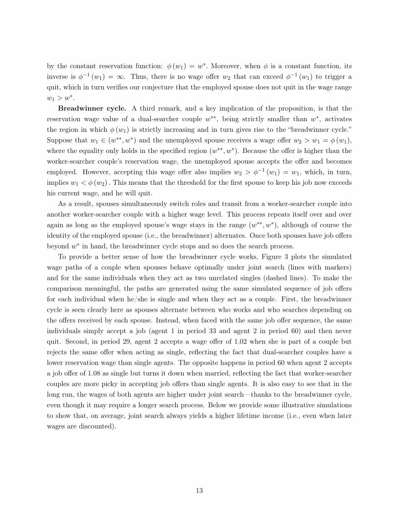
To provide a better sense of how the breadwinner cycle works, Figure 3 plots the simulatedwage paths of a couple when spouses behave optimally under joint search (lines with markers)and for the same individuals when they act as two unrelated singles (dashed lines). To make thecomparison meaningful, the paths are generated using the same simulated sequence of job offersfor each individual when he/she is single and when they act as a couple. First, the breadwinnercycle is seen clearly here as spouses alternate between who works and who searches depending onthe offers received by each spouse. Instead, when faced with the same job offer sequence, the sameindividuals simply accept a job (agent 1 in period 33 and agent 2 in period 60) and then neverquit. Second, in period 29, agent 2 accepts a wage offer of 1.02 when she is part of a couple butrejects the same offer when acting as single, reflecting the fact that dual-searcher couples have alower reservation wage than single agents. The opposite happens in period 60 when agent 2 acceptsa job offer of 1.08 as single but turns it down when married, reflecting the fact that worker-searchercouples are more picky in accepting job offers than single agents. It is also easy to see that in thelong run, the wages of both agents are higher under joint search—thanks to the breadwinner cycle,even though it may require a longer search process. Below we provide some illustrative simulationsto show that, on average, joint search always yields a higher lifetime income (i.e., even when laterwages are discounted).

13

Figure 3: Simulated Wage Paths for a Couple and for the Same Individuals When They Are Single

0 20 40 60 80 100 120 140 160 180 200

0.4

0.6

0.8

1

1.2

Time (weeks)

Wag

e

0 20 40 60 80 100 120 140 160 180 200

0.4

0.6

0.8

1

1.2

Time (weeks)

Wag

e

Single 2

Spouse 2

Single 1

Spouse 1

3.3.2 DARA utility

As noted earlier, DARA utility is of special interest, since it encompasses the well-known andcommonly used CRRA utility specification u (c) = c1−ρ/ (1− ρ). More generally, the coefficient ofabsolute risk aversion with DARA preferences is −u′′ (c) /u′ (c) = ρ/(c+ ρa), which decreases withthe consumption (and hence the wage) level. The following proposition characterizes the optimalsearch strategy for couples with DARA preferences.

Proposition 3 [DARA utility] With DARA preferences, the search behavior of a couple can becharacterized as follows:

(i) The reservation wage value of a dual-searcher couple satisfies: w∗∗ < w (with w∗ < w), whichimplies that the breadwinner cycle exists.

(ii) The reservation wage function of a worker-searcher couple has the following properties: forw1 < w, φ (w1) = w1, and for w1 ≥ w, φ (w1) is strictly increasing with φ′ < 1.

Figure 4 provides a graphical representation of the reservation wage functions associated withthe DARA case. Unlike the CARA case, the reservation function of the worker-searcher coupleis now increasing with the wage of the employed spouse at all wage levels. This is because withdecreasing absolute risk aversion, a couple becomes less concerned about smoothing consumptionas household resources increase and, consequently, becomes more picky in its job search.

Again, it is useful to sketch the main idea behind the proof, which proceeds by assuming a non-increasing reservation wage function and showing that this leads to a contradiction. Specifically,

14

begin by supposing that φ′ (·) ≤ 0 beyond a certain wage threshold. In this range, the quit optionwill not be exercised, so we have

u (w1 + φ (w1))− u (w1 + b) =α

r

∫φ(w1)

[u (w1 + w2)− u (w1 + φ (w1))] dF (w2) ,

which is identical to the CARA case, except that we have rearranged the terms here for convenience.Divide both sides by the left-hand side:

1 =α

r

∫φ(w1)

[u (w1 + w2)− u (w1 + φ (w1))u (w1 + φ (w1))− u (w1 + b)

]dF (w2) . (13)

Now consider a wage level w1 > w1 and replace φ (w1) on the right-hand side with φ (w1) (whichis smaller, by our hypothesis that φ′ (·) ≤ 0). Then we have

1 ≤ α

r

∫φ(w1)

[u (w1 + w2)− u (w1 + φ(w1))u (w1 + φ(w1))− u (w1 + b)

]dF (w2) . (14)

Next, applying a well-known result on DARA preferences established by Pratt (1964, Theorem1), it can easily be shown that the following inequality holds for any p > m > q and w1 > w1 :

u (w1 + p)− u (w1 +m)u (w1 +m)− u (w1 + q)

<u (w1 + p)− u (w1 +m)u (w1 +m)− u (w1 + q)

. (15)

Setting p ≡ w2,m ≡ φ(w1), and , integrating both sides over w2, and then combining withequation (14) yields

1 <α

r

∫φ(w1)

[u (w1 + w2)− u (w1 + φ(w1))u (w1 + φ(w1))− u (w1 + b)

]dF (w2) .

But notice that the right-hand side of this last expression and of equation (13) are identical(when w1 is replaced with w1), whereas the left-hand side of each expression is different. Therefore,we have reached a contradiction, establishing that φ′ (w1) > 0 as stated in the proposition.

The proposition also shows that the breadwinner cycle continues to exist. In contrast to theCARA case, now the breadwinner cycle is observed over a wider range of wage values of the employedspouse. This is because, as can be seen in Figure 4, φ is strictly increasing in w1, so its inverse isnot a vertical line anymore but is itself an increasing function. As a result, even when w1 > w, asufficiently high wage offer—one that exceeds φ−1 (w1)—not only will be accepted by the unemployedspouse but will also trigger the employed spouse to quit. One way to understand this result is bynoting that the employed spouse will quit if his reservation wage upon quitting is higher than hiscurrent wage. If w2 > φ−1 (w1), this implies that upon quitting the job, the reservation wage forthe currently employed spouse becomes φ (w2) > φ

(φ−1 (w1)

)= w1. Since this reservation wage is

higher than his current wage, it is optimal for the employed spouse to quit the job. Note that onlyif the wage offer is w2 ∈

(φ (w1) , φ−1 (w1)

), the job offer is accepted without triggering a quit.

Finally, there is an interesting analogy between our result that φ′ (w1) > 0 with DARA anda recent finding in search models of marriage formation. Consider a special case of our model

15

Figure 4: Reservation Wage Functions with DARA Preferences

where unemployment income is zero and where job quits are not allowed. A worker-searcher couplecan be thought of as a single individual with endowment w1 looking for another individual withendowment w2 in order to form a marriage with total endowment w1 +w2 (e.g., Visschers, 2006). Inthis environment, if individuals (single or married) use DARA utility to value endowments, positiveassortative matching along the w dimension occurs. This means precisely that φ′ (w1) > 0.

3.3.3 IARA utility

We now turn to IARA preferences, which display increasing absolute risk aversion as consumptionincreases. One well-known example of IARA preferences is quadratic utility: − (c− c)2, where c isthe bliss point.

Proposition 4 [IARA utility] With IARA preferences, the search behavior of a couple can becharacterized as follows:

(i) The reservation wage value of a dual-searcher couple satisfies: w∗∗ < w, which implies thatthe breadwinner cycle exists.

(ii) The reservation wage function of a worker-searcher couple has the following properties: forw1 < w, φ (w1) = w1, and for w1 ≥ w, φ (w1) is strictly decreasing.

The proof of the proposition is very similar to the DARA case and is therefore omitted forbrevity.9 Figure 5 graphically shows the IARA case.

9The logic of the proof is as follows. Conjecture that beyond some wage level w1 the employed worker never quits,and verify the guess by using the property of IARA (also shown by Pratt (1964)) corresponding to (15), but with theinequality reversed. The rest of the proof is exactly as for the DARA case.

16

Figure 5: Reservation Wage Functions with IARA Preferences

The reservation wage function φ of a worker-searcher couple deviates from the CARA benchmarkin the opposite direction of the DARA case. In particular, beyond wage level w, the reservationfunction φ (w1) is decreasing in w1, whereas it was increasing in the DARA case. As a result, if theunemployed spouse receives a wage offer higher than φ−1 (w1), she accepts the offer, the employedstays in the job, and both stay employed forever. If the wage offer instead is between φ (w1) andφ−1 (w1), then the job offer is accepted followed by a quit by the employed spouse. This behavior isthe opposite of the DARA case where high wage offers resulted in quit and intermediate wages didnot. Moreover, now the breadwinner cycle never happens at wage levels w1 > w. This is a directconsequence of increasing absolute risk aversion, which induces a couple to become less choosy whensearching as its wage level rises.

Before concluding this section, it is interesting to ask why it is that the absolute risk aversiondetermines the properties of joint-search behavior (as shown in the propositions so far), as opposedto, for example, relative risk aversion. The reason is that individuals are drawing wage offers fromthe same probability distribution regardless of the current wage earnings of the couple. As a result,the uncertainty they face is fixed and is determined by the dispersion in the wage offer distribution,making the attitudes of a couple toward a fixed amount of risk—and therefore, the absolute riskaversion—the relevant measure.10

3.4 An isomorphism: search with multiple job holdings

The joint-search framework analyzed so far is isomorphic to a search model with a single agent whocan hold multiple jobs at the same time. To see this, suppose that the time endowment of a workercan be divided into two subperiods (e.g., day shift and night shift). The single agent can be (i)

10If, for example, individuals were to draw wage offers from a distribution that depended on the current wage of acouple, this would make relative risk aversion relevant as well.

17

unemployed and searching for his first job while enjoying 2b units of home production, (ii) workingone job at wage w1 while searching for a second one, or (iii) holding two jobs with wages w1 and w2.

It is easy to see that the problem faced by this individual is exactly given by the same equations((4), (5), and (6)) for the joint-search model and therefore has the same solution.11

Consequently, for example, when the agent works in one job and gets a second job offer with asufficiently high wage offer, he will accept the offer and simultaneously quit the first job to searchfor a better one. In this case, it is not the breadwinner that alternates, but the jobs that the workerjuggles over time.

4 Extensions

The baseline joint-search framework we developed up to this point is intended to provide the simplestpossible deviation from the well-known single-search problem. Despite being highly stylized, thissimple model illustrated some new and potentially important mechanisms that are not operationalin the single-agent search problem.

In this section, we enrich this basic model in four empirically relevant directions. First, weallow for nonparticipation. Second, we add on-the-job search. Third, we allow for exogenous jobseparations. Fourth, we allow households to borrow in financial markets. In a number of specialcases, we are able to fully characterize the reservation strategies of the couple. We also simulate acalibrated version of our model to analyze the differences between a single-agent search economyand the joint-search economy in more general cases.

4.1 Nonparticipation

We now extend the two-state model of the labor market we adopted so far to a three-state modelwhere either spouse can choose nonparticipation. Nonparticipation means that the individual doesnot search for a job opportunity. Consistently with the rest of the paper, where we interpret bas income, we model the benefit associated to nonparticipation as z > b consumption units (e.g.,through home production).

We need to redefine some of the value functions for the couple. First, consider the two configu-rations where (i) both spouses are outside the labor force, and (ii) one spouse does not participateand the other is employed at wage w. Because of the absence of randomness, both of these statesare absorbing, as they are for the dual-worker couple. Therefore, we can denote the flow valuefor a couple in the first state as rT (z, z) = u (2z) and the flow value for a couple in the secondstate as rT (z, w2) = u (z + w2) . This formulation shows that nonparticipation is equivalent to ajob opportunity which pays z (and entails foregoing search) that is always available to the worker.

11There is a further implicit assumption here: the arrival rate of job offers is proportional to the nonworking timeof the agent (that is, 2α when unemployed and α when working one job).

18

The flow value for the state where one spouse does not participate and the other is unemployedis

rΩ (z) = u (z + b) + α

∫max T (z, w2)− Ω (z) ,Ω (w2)− Ω (z) , 0 dF (w2) , (16)

where the equation shows that upon spouse 2 accepting a job offer, spouse 1 can either remain outof the labor force, or start searching.

The value of a dual-searcher couple becomes

rU = u (2b) + 2α∫

max T (z, w)− U,Ω (w)− U, 0 dF (w) , (17)

which shows that upon either spouse finding a job, the other has the choice of either continuing tosearch or dropping out of the labor force.

Finally, the value of a worker-searcher couple where spouse 1 is employed is

rΩ (w1) = u (w1 + b) + α

∫max T (w1, w2)− Ω (w1) ,Ω (w2)− Ω (w1) , 0 dF (w2) . (18)

The choices available to the couple when spouse 2 finds an acceptable job offer are either spouse1 remains employed at w1 or spouse 1 quits into unemployment. This state will arise only forw1 > z, since z is always available.12 As clear from this equation, once the couple reaches this state,nonparticipation will never occur thereafter. This observation is important, since it means that ourdefinitions of w∗∗, w, and φ (w) remain unchanged and these functions are independent of z.

Proposition 5 [Joint search with nonparticipation] With either CARA or DARA preferences,the search behavior of a couple can be characterized as follows:

(i) If z ≤ w∗∗, the search strategy of the couple is unaffected by nonparticipation, since the latteroption is never optimal.

(ii) If w∗∗ < z < w, dual search is never optimal, and whenever a spouse is unemployed, the otheris either employed or a nonparticipant. The reservation wage of a nonparticipant-searchercouple is z, and the reservation function of a worker-searcher couple is the same functionφ (w) as in the absence of nonparticipation.

(iii) If z ≥ w, nonparticipation is an absorbing state for both spouses, and search is never optimal.

Since nonparticipation is like a job offer at wage z that is always available, if z < w∗∗ suchoffer is never accepted by a dual-searcher couple, and nonparticipation is never optimal. Whenw∗∗ < z < w, then consumption-smoothing motives induce the jobless couple to move one of itsmembers into nonparticipation—say, spouse 1—while spouse 2 is searching with reservation wage

12More precisely, there is a third option in the max operator which is, theoretically, available to spouse 1: quittinginto nonparticipation and accepting z forever with a gain T (z, w2)− Ω (w1) for the couple. However, the wage gainassociated with spouse 1 keeping his/her current job, T (w1, w2)− Ω (w1), must be larger, since previously spouse 1has accepted w1 when z was available.

19

φ (z) = z. As soon as a wage offer w2 larger than z arrives, the unemployed spouse accepts thejob and spouse 1 switches into unemployment, since search is equivalent to being employed atφ (w2) ≥ w > z. The first inequality follows from the CARA or DARA assumption under which φis a nondecreasing function. It is immediate that if z ≥ w, then both spouses exit the labor forceright away and no search occurs. As soon as one chooses not to search, the other spouse reservationwage becomes φ (z), which is always smaller than z in this region. As a result, nonparticipation isattractive for the other spouse as well.13

The joint-search problem is, once again, different from the single-agent search problem. Forexample, in the CARA case where w = w∗, we can establish that under configuration (ii), a singleagent would be always searching and nonemployment would never arise, whereas a jobless couplewould choose to move one spouse out of the labor force for consumption-smoothing purposes.

Finally, note that under this representation of nonparticipation as income, we obtain a starkresult: the couple will never be in a state where one spouse works and the other is a nonparticipant.14

However, the next lemma shows that under IARA, the worker-nonparticipant configuration may beoptimal for the couple. Intuitively, since φ is decreasing in w (recall Figure 5), a wage offer w couldarrive—say, to a dual searcher couple—that is, high enough to induce the couple to accept the offerand set the new reservation wage for the unemployed member to φ (w) < z. Thus, the unemployedmember immediately exits the labor force.

Lemma 2 [Non participation with IARA preferences] With IARA preferences, both dualsearcher couples and non-participant searcher couples can become non-participant worker couples.

4.2 On-the-job search

Suppose that agents can search both off and on the job. During unemployment, they draw a newwage from F (w) at rate αu, whereas during employment they sample new job offers from the samedistribution F at rate αe. What we develop below is, essentially, a version of the Burdett (1978)wage ladder model with couples. The flow value functions in this case are

rU = u (2b) + 2αu∫

max Ω (w)− U, 0 dF (w) , (19)

rΩ (w1) = u (w1 + b) + αu

∫max T (w1, w2)− Ω (w1) ,Ω (w2)− Ω (w1) , 0 dF (w2) (20)

+ αe

∫max

Ω(w′1)− Ω (w1) , 0

dF(w′1),

13In order to save space, we do not represent graphically this version of the model. It is immediate to see that onecan generate the graph with nonparticipation corresponding to case (ii) by overlapping a squared area with coordinates(x, y) = (z, z) to Figures 2 and 4. This area would substitute the dual-searcher couple with the nonparticipant-searchercouple.

14If preferences are CARA or DARA, this state can only occur when wealth effects on labor supply are active (asin Burdett and Mortensen, 1977), or in presence of asymmetries between spouses.

20

rT (w1, w2) = u (w1 + w2) + αe

∫max

T(w′1, w2

)− T (w1, w2) , 0

dF(w′1)

(21)

+ αe

∫max

T(w1, w

′2

)− T (w1, w2) , 0

dF(w′2).

We continue to denote the reservation wage of the dual-searcher couple as w∗∗ and the reservationwage of the unemployed spouse in the worker-searcher couple as φ (w1) . We now have a new reser-vation function, that of the employed spouse (in the dual-worker couple and in the worker-searchercouple) which we denote by η (wi) .

It is intuitive (and can be proved easily) that under risk neutrality the joint-search problemcoincides with the problem of the single agent regardless of offer arrival rates. Below, we proveanother equivalence result that holds for any risk-averse utility function but for the special case ofsymmetric offer arrival rates αu = αe, i.e., when search is equally effective on and off the job.

Proposition 6 [On-the-job search with symmetric arrival rates] If αu = αe, the joint-searchproblem yields the same solution as the single-agent search problem, even with concave preferences.Specifically, w∗∗ = w∗ = b, φ (w1) = w∗∗ and η (wi) = wi for i = 1, 2.

To understand this equivalence result, notice that one way to think about joint search is thatit provides a way to climb the wage ladder for the couple even without on-the-job search: whena dual-searcher couple accepts the first job offer, it continues to receive offers, albeit at a reducedarrival rate. Therefore, one can view joint search as a “costly” version of on-the-job search. The costcomes from the fact that, absent on the job search, in order to keep the search option active, the pairmust remain a worker-searcher couple and must not enjoy the full wage earnings of a dual-workercouple as it would be capable of doing with on-the-job search. As a result, when on-the-job searchis explicitly introduced and the offer arrival rate is equal across employment states, it completelyneutralizes the benefits of joint search and makes the problem equivalent to that of a single agent.The solution is then simply that the unemployed partner should accept any offer above b and thespouse employed at w1 any wage above its current one.

The preceding proposition that characterizes joint-search behavior when αu = αe provides analternative benchmark to the baseline model, which had αu > αe ≡ 0. The empirically relevant caseis probably in between these two benchmarks, in which case joint-search behavior continues to bequalitatively different from single search (for example, the breadwinner cycle will be active). Weprovide some simulations in Section 4.5 below to illustrate these intermediate cases.

Empirically, one would expect the network of labor market contacts and opportunities (and hencethe effectiveness of on-the-job search) to increase with skill level and with occupational experience.As a result, deviations from single-agent search should be more evident among young, inexperienced,and uneducated couples.

21

4.3 Exogenous separations

As discussed above, in the absence of exogenous separations, agents optimally choose not to ac-cumulate assets, so a simple no-borrowing constraint ensures that agents live as hand-to-mouthconsumers. This is no longer true when exogenous separation risk is introduced, because in thiscase accumulated assets can be used to smooth consumption when agents lose their jobs. This savingmotive, however, significantly complicates the analysis. Thus, to establish some general theoreticalresults, we rule out storage in this section.

Suppose that jobs are exogenously lost at rate δ and that upon a job loss, workers enter unem-ployment. Once again, under risk neutrality it is easy to establish that the joint-search problemcollapses to the single-agent problem. With risk aversion, however, this is not the case anymore.We first state the following proposition that characterizes joint-search behavior with exogenous sep-arations and then discuss the intuition. The modifications to the value functions are immediate, sowe omit them.

Proposition 7 [CARA/DARA utility with exogenous separations] With CARA or DARApreferences, no access to financial markets, and exogenous job separation, the search behavior of acouple can be characterized as follows:

(i) The reservation wage value of a dual-searcher couple satisfies: w∗∗ < w (with w∗ < w), whichimplies that the breadwinner cycle exists.

(ii) The reservation wage function of a worker-searcher couple has the following properties: forw1 < w, φ (w1) = w1, and for w1 ≥ w, φ (w1) is strictly increasing with φ′ < 1.

Two remarks are in order. First, for DARA preferences, the existence of exogenous separationshas qualitatively no effect on joint-search behavior, as can be seen by comparing Propositions 3 and7.15 Second, and perhaps more interestingly, for CARA preferences φ (w1) is no longer independentof the employed spouse’s wage but is now increasing with it. In the context of joint-search, theseparation risk has two separate meanings. Consider the problem of the worker-searcher couplewith current wage w1 contemplating a new job offer with wage w2. First, there is the risk associatedwith the duration of the new job offered to the searching spouse. Second, there is the risk of jobloss for the currently unemployed spouse.16

The first effect of exogenous separations is also present in the single-agent search model: if theexpected duration of a job is lower (high δ), the unemployed agent reduces her reservation wage forall values of w1. However, the larger the wage w1 of the employed spouse, the smaller this effect,since the utility value for the household of the additional wage decreases in w1. Since φ (w1) is

15The only difference is that here we explicitly rule out saving, whereas previous propositions did not require thisassumption as explained before. However, apart from the stronger assumption made here, the search behavior withDARA utility is the same in the two propositions.

16In a model with spouse asymmetries in separation rates, this would be even more clear, since we would have apair (δ1, δ2) in the value functions as opposed to just δ.

22

weakly decreasing in the case δ = 0, with δ > 0 the reservation function φ (w1) will become strictlyincreasing.

The second effect is related to the event that the currently employed spouse might lose his job.If the couple turns down the offer at hand and the job loss indeed occurs, its earnings will fall fromw1 + b to 2b for a net change of b − w1 < 0. Clearly, this income loss (and, therefore, the fall inconsumption) is larger, the higher is the current wage of the employed spouse. If instead the coupleaccepts the job offer and spouse 1 loses his job, earnings will change from w1 + b to b+w2, for a netchange of w2−w1. On the one hand, setting the reservation wage to φ (w1) = w1 would completelyinsure the downside risk of spouse 1 losing his job (because then w2 − w1 ≥ 0). At the same time,letting the reservation wage rise this quickly with w1 reduces the probability of an acceptable offerand increases the probability that the searcher will still be unemployed when spouse 1 loses his job.As a result, the optimal reservation wage policy balances these two considerations to provide thebest self-insurance to the couple and, consequently, have φ (w1) rise with w1, but less than one forone: φ′ < 1.17

4.4 Borrowing in financial markets

With few exceptions, search models with risk-averse agents and a borrowing-saving decision do notallow analytical solutions.18 One such exception is when preferences display CARA and agentshave access to a risk-free asset. This environment has been recently used in previous work toobtain analytical results in the context of the single-agent search problem (e.g., Acemoglu andShimer (1999), and Shimer and Werning (2008)). Following this tradition, we start from the CARAframework studied in Section 3.3.1, extended to allow for borrowing. Before analyzing the joint-search problem, it is useful to recall here the solution to the single-agent problem.

Single-agent search problem. Let a denote the asset position of the individual. Assets evolveaccording to the law of motion,

da

dt= ra+ y − c, (22)

where r is the risk-free interest rate, y is income (equal to w during employment and b duringunemployment), and c is consumption. The value functions for the employed and unemployedsingle agent are, respectively:

rW (w, a) = maxcu (c) +Wa (w, a) (ra+ w − c) , (23)

rV (a) = maxcu (c) + Va (a) (ra+ b− c)+ α

∫max W (w, a)− V (a) , 0 dF (w) , (24)

17This mechanism is closely related to Lise (2006), in which individuals climb the wage ladder but fall to the sameunemployment benefit level upon layoff. As a result, in his model, the savings rate increases with the current wagelevel, whereas this increased precautionary savings demand manifests itself as delayed offer acceptance in our model.

18Some examples in which the decision maker is an individual are Costain (1999), Browning, Crossley, and Smith(2003), Lentz (2009), Lentz and Tranaes (2005), Rendon (2006), Lise (2006), Krusell et al. (2007), and Rudanko(2008).

23

where the subscript denotes the partial derivative. These equations reflect the nonstationarity dueto the change in assets over time. For example, the second term in the RHS of (23) is (dW/dt) =(dW/da) · (da/dt). And similarly for the second term in the RHS of (24).

We begin by conjecturing that rW (w, a) = u (ra+ w) . If this is the case, then the first-ordercondition (FOC) determining optimal consumption for the agent gives u′ (c) = u (ra+ w), whichconfirms the conjecture and establishes that the employed individual consumes his current wageplus the interest income on the risk-free asset. Let us now guess that rV (a) = u (ra+ w∗) . Oncegain, it is easy to verify this guess through the FOC of the unemployed agent. Substituting thissolution back into equation (24) and using the CARA assumption yields

w∗ = b+α

ρr

∫w∗

[u (w − w∗)− 1] dF (w) , (25)

which shows that w∗ is the reservation wage and is independent of wealth. Therefore, the unem-ployed worker consumes the reservation wage plus the interest income on his wealth. This resulthighlights an important point: the asset position of an unemployed worker deteriorates and, inpresence of a debt constraint, she may hit it. As in the rest of the papers cited above which usethis setup, we abstract from this possibility. The implicit assumption is that borrowing constraintsare “loose,” and by this we mean they do not bind along the solution for the unemployed agent.

Joint-search problem. When the couple searches jointly for jobs, the asset position of thecouple still evolves based on (22), but now y = 2b for the dual-searcher couple, b + w1 for theworker-searcher couple, and w1 + w2 for the employed couple. The value functions become

rT (w1, w2, a) = maxcu (c) + Ta (w1, w2, a) (ra+ w1 + w2 − c) , (26)

rU (a) = maxcu (c) + Ua (a) (ra+ 2b− c)+ α

∫max Ω (w, a)− U (a) , 0 dF (w) , (27)

rΩ (w1, a) = maxcu (c) + Ωa (w1, a) (ra+ w1 + b− c) (28)

+ α

∫max T (w1, w2, a)− Ω (w1, a) ,Ω (w2, a)− Ω (w1, a) , 0 dF (w2) .

Solving this problem requires characterizing the optimal consumption policy for the dual-searchercouple cu (a), for the worker-searcher couple ceu (w1, a), and for the dual-worker couple ce (w1, w2, a) ,as well as the reservation wage functions, now potentially a function of wealth too, which must sat-isfy, as usual: Ω (w∗∗ (a) , a) = U (a), T (w1, φ (w1, a) , a) = Ω (w1, a), and Ω (φ (w1) , a) = Ω (w1, a).The following proposition characterizes the solution to this problem.

Proposition 8 [CARA utility and access to financial markets] With CARA preferences,access to risk-free borrowing and lending, and “loose” debt constraints, the search behavior of acouple can be characterized as follows:

(i) The optimal consumption policies are: cu (a) = ra + 2w∗∗, ceu (w1, a) = ra + w∗∗ + w1, andce (w1, w2, a) = ra+ w1 + w2.

24

(ii) The reservation function φ of the worker-searcher couple is independent of (w1, a) and equalsw∗∗, so there is no breadwinner cycle.

(iii) The reservation wage w∗∗ of the dual-searcher couple equals w∗, the reservation wage of thesingle-agent problem.

The main message of this proposition could perhaps be anticipated by the fact that borrowingeffectively substitutes for the consumption smoothing provided within the household, making thelatter redundant. Each spouse can implement search strategies that are independent from the otherspouse’s actions and, as a result, each acts as in the single-agent model. Of course, to the extentthat borrowing constraints bind or preferences deviate from CARA, the equivalence result no longerapplies.

The sharp contrast between the baseline model with no borrowing and this model with loose debtlimits provides a useful guide for future empirical work. In particular, it suggests that deviationsfrom single-agent search behavior in the data (such as the breadwinner cycle) are more likely to bedetectable among young and poor households and may be less significant among older and wealthierhouseholds. Interestingly, we reached the same conclusion in Section 4.2, where we proved another“equivalence result” between single-agent and joint search in the presence of on-the-job search.

4.5 Some illustrative simulations

In this section, our goal is to gain some sense about the quantitative differences in labor marketoutcomes between the single-search and the joint-search economy. We start from the case of CRRAutility and exogenous separations. Later we add on-the-job search. Thus, the economy is character-ized by the following set of parameters: b, r, ρ, δ, F, αu, αe. When on-the-job search is not allowed,we simply set αe = 0 and α ≡ αu.

We first simulate labor market histories for a large number of individuals acting as singles,then compute their optimal choices and some key statistics: the reservation wage w∗, the meanwage, the unemployment rate, and unemployment duration. Second, we pair individuals togetherand treat them as couples solving the joint-search problem in exactly the same economy (i.e.,same set of parameters). We use the same sequence of wage offers and separation shocks in botheconomies. The interest of the exercise lies in comparing the key labor market statistics acrosseconomies. For example, it is not obvious whether the joint-search model would have a higher orlower unemployment rate: for the dual-searcher couples, w∗∗ < w∗, but for the worker-searchercouple φ (w) is above w∗ at least for large enough wages of the employed spouse.

Calibration. We calibrate the model to replicate the salient features of the US economy. Thetime period in the model is set to one week of calendar time. The coefficient of relative risk aversionρ will vary from zero (risk neutrality) up to eight in simulations. The weekly net interest rate,r, is set equal to 0.001, corresponding to an annual interest rate of 5.3%. Wage offers are drawn

25

Table 1: Single versus Joint Search: CRRA Preferences

ρ = 0 ρ = 2 ρ = 4 ρ = 8Single Joint Single Joint Single Joint Single Joint

Res. wage w∗/w∗∗ 1.02 1.02 0.98 0.75 0.81 0.58 0.60 0.48Res. wage φ (1) − n/a − 1.03 − 0.941 − 0.84Double ind. w − 1.02 − 1.02 − 0.94 − 0.82Mean wage 1.06 1.06 1.07 1.10 1.01 1.05 1.001 1.01Mm ratio 1.04 1.04 1.09 1.47 1.23 1.81 1.67 2.10Unemp. rate 5.5% 5.5% 5.4% 7.6% 5.4% 7.7% 5.3% 5.6%Unemp. duration 9.9 9.9 9.7 12.6 9.8 13.3 9.6 10

Dual-searcher − 6 − 4.7 − 7.7 − 7.1Worker-searcher − 9.8 − 14.2 − 13.6 − 9.6

Job quit rate − 0% − 11.1% − 5.55% − 0.74%EQVAR- cons. − 0% − 4.5% − 14% − 26%EQVAR- income − 0% − 1.1% − 2.8% − 0.7%

from a log-normal distribution with standard deviation σ = 0.1 and mean µ = −σ2/2 so that theaverage wage is always normalized to one. We set δ = 0.0054, which corresponds to a monthlyemployment-unemployment (exogenous) separation rate of 0.02. For each risk aversion value, theoffer arrival rate, αu, is recalibrated to generate an unemployment rate of roughly 0.055.19 Forthe model with on-the-job search, we set the offer arrival rate on the job, αe, to match a monthlyemployment-employment transition rate of 0.02. Finally, the value of leisure b is set to 0.40 , i.e.,40% of the mean of the wage offer distribution.

Table 1 reports the results of our simulation. The first two columns confirm the statementin Proposition 1 that under risk neutrality the joint-search problem reduces to the single-searchproblem. Let us now consider the case with ρ = 2. The reservation wage of the dual-searchercouple is almost 25% lower than in the single-search economy. And this is reflected in the muchshorter unemployment durations of dual-searcher couples. At the same time, though, the reservationwage of worker-searcher couples is always higher than w∗. In the second row of the table, wereport the reservation wage of the worker-searcher couple at the mean wage offer. Indeed, for thesecouples, unemployment duration is higher. Overall, this second effect dominates and the joint-search economy displays a longer average unemployment duration—12.6 weeks instead of 9.7—anda considerably higher unemployment rate, 7.6% instead of 5.4%.

Comparing the mean wage tells a similar story. The job-search choosiness of worker-searcher19As risk aversion goes up, w∗∗ falls and unemployment duration decreases. So, to continue matching an unem-

ployment rate of 5.5%, we need to decrease the value of αu. For example, for ρ = 0, αu = 0.4 and for ρ = 8,αu = 0.12.

26

couples dominates the insurance motive of dual-searcher couples, and the average wage is higher inthe joint-search model. The ability of the couple to climb higher up the wage ladder is reflected inthe endogenous quit rate (leading to the breadwinner cycle), which is sizeable, 11.1%. Indeed, theregion in which the breadwinner cycle is active is rather big, as measured by the gap between w∗∗

and w, which is equal to 2.7 times the standard deviation of the wage offer.The next six columns in Table 1 display how these statistics change as we increase the coefficient

of relative risk aversion. As is clear from the first row, in the case when ρ = 0 the difference betweenw∗ and w∗∗ is zero. As ρ goes up, both reservation wages fall. Clearly, higher risk aversion impliesa stronger demand for consumption smoothing, which makes the agent accept a job offer morequickly. However, the gap between w∗ and w∗∗ first grows but then shrinks. Indeed, as ρ → ∞, itmust be true that w∗ = w∗∗ = b, so the two economies converge again. As for φ (1), it falls as riskaversion increases, which means that for higher values of ρ, the worker-searcher couple accepts joboffers more quickly, thus reducing unemployment. Indeed, at ρ = 8 the unemployment rate and themean wage are almost the same in the two economies.

We also report a measure of frictional wage dispersion, the mean-min ratio (Mm), defined as theratio between the mean wage and the lowest wage, i.e., the reservation wage. Hornstein, Krusell,and Violante (2006) demonstrate that the sequential search model with homogeneous workers, whenplausibly calibrated, generates very little frictional wage dispersion. The fifth row of Table 1 confirmsthis result. It also confirms the finding in Hornstein et al. that the Mm ratio increases with riskaversion. What is novel here is that the joint-search model generates more frictional dispersion: thereservation wage for the dual-searcher couple is lower, but the couple can climb the wage distributionfaster which translates into a higher average wage.

Next, we discuss two separate measures of the welfare effects of joint search in the simulatedeconomy. Recall that the jointly searching couple has two advantages: first, it can smooth con-sumption better, and second, it can get higher earnings. The first measure of welfare gain is thestandard consumption-equivalent variation and embeds both advantages. The second is the changein lifetime income from being married, which isolates the second aspect—the novel one.20 Theconsumption-based measure of welfare gain is very large, not surprisingly. What is remarkable isthat also the gains in terms of lifetime income can be very large—for example, around 2.8% for thecase ρ = 4. As risk aversion goes up, the welfare gains from family insurance keep increasing, butas explained above, the ones stemming from better search opportunities fade away.

Table 2 presents the results when on-the-job search is introduced into this environment. The firstfour columns simply confirm the theoretical results established in previous sections. For example,when agents are risk neutral, on-the-job search has no additional effect, and both the single- andjoint-search problems yield the same solution regardless of parameter values. Similarly, as shownin Proposition 6 when on-the-job search is as effective as search during unemployment (αe = αu),

20To make the welfare comparison between singles and couples meaningful, we assume that each spouse consumeshalf of the household’s income (as opposed to “all income” assumed in the theoretical analysis). Notice that, withpreferences used here, this alternative assumption does not affect any of our theoretical results.

27

Table 2: Single versus Joint Search: CRRA Preferences and On-the-Job Search

ρ = 0 ρ = 2 ρ = 2 ρ = 4αu = 0.2, αe = 0.03 αu = 0.1, αe = 0.1 αu = 0.11, αe = 0.02 αu = 0.11, αe = 0.02Single Joint Single Joint Single Joint Single Joint

Res. wage w∗/w∗∗ 0.98 0.98 0.4 0.4 0.78 0.67 0.62 0.54Res. wage φ (1) − 0.98 − 0.4 − 0.85 − 0.74Double ind. w − 0.98 − 0.4 − 0.87 − 0.8Mean wage 1.13 1.13 1.16 1.16 1.08 1.09 1.08 1.09Mm ratio 1.15 1.15 2.90 2.90 1.38 1.63 1.74 2.02Unemp. rate 5.4% 5.4% 5.4% 5.4% 5.3% 5.8% 5.3% 5.4%Unemp. duration 9.8 9.8 10.5 10.5 9.7 10.6 9.6 9.8

Dual-searcher − 7 − 7.7 − 7.1 − 7Worker-searcher − 9.4 − 9.9 − 10.2 − 9.3

EU quit rate − 0% − 0% − 0.93% − 0.19%EE transition 0.45% 0.45% 1.03% 1.03% 0.49% 0.47% 0.51% 0.49%EQVAR-cons. − 0% − 4.6% − 4.1% − 15%EQVAR-income − 0% − 0% − 0.2% − 0.05%

then, again, single and joint search coincide.Overall, comparing these results to those in Table 1 shows that the effects of joint search on labor

market outcomes are qualitatively the same as before, but they become much smaller quantitatively.This is perhaps not surprising in light of the discussion in Section 4, where we argued that jointsearch is a partial substitute for on-the-job search (or a costly version of it). Therefore, once on-the-job search is available, having a search partner is not so useful any longer to obtain higher earnings.But it obviously remains an effective means to smooth consumption, as evident from the last twolines of the table.

5 Joint Search with Multiple Locations

The importance of the geographical dimension of job search is undeniable. For the single-agentsearch problem, accepting a job in a different market could require a relocation cost that may behigh enough to induce the agent to turn down the offer. In the joint-search problem, the spatialdimension introduces a new and interesting search friction. In addition to migration costs that alsoapply to a single agent, a couple is likely to suffer from the disutility of living apart if spouses acceptjobs in different locations. This cost can easily rival or exceed the physical costs of relocation, sinceit is a flow cost as opposed to the latter, which are arguably better thought of as one-time costs.

To analyze the joint-search problem with multiple locations, we extend the framework proposed

28

in Section 2 by introducing a fixed flow cost of living separately for a couple. As we shall seebelow, the introduction of location choice leads to several important changes in the search behaviorof couples compared to a single agent, even with risk neutrality. For this reason, below we focuson the risk-neutral case. Furthermore, many of these changes are not favorable to couples, whichserves to show that joint search can itself create new frictions. This is in contrast to the analysisperformed so far, which only showed new opportunities of joint search.21

To keep the analysis tractable, we first consider agents that search for jobs in two symmetriclocations and provide a theoretical characterization of the solution. In the next subsection, we ex-amine the more general case with L(> 2) locations that is more suitable for a meaningful calibrationand provide some results based on numerical simulations.

5.1 Two locations

Environment. A couple is an economic unit composed of a pair of risk-neutral spouses (1, 2). Theeconomy has two locations. Couples incur a flow resource cost, denoted by κ, if the two spouses liveapart. Denote by i the “inside” location, i.e., the location where the couple resides, and by o the“outside” location. Offers arrive at rate αi from the current location and at rate αo from the outsidelocation, e.g., job search in the inside location is more effective. The two locations have the samewage offer distribution F. We assume away moving costs: the aim of the analysis is the comparisonwith the single-agent problem, and such costs would also be borne by the single agent.

A couple can be in one of four labor market states. First, if both spouses are unemployed andsearching, they are referred to as a “dual-searcher couple.” Second, if both spouses are employedin the same location (in which case they will stay in their jobs forever) we refer to them as a“dual-worker couple,” but if they are employed in different locations we refer to them as a “separatedual-worker couple” (another absorbing state). Finally, if one spouse is employed and the otherone is unemployed, we refer to them as a “worker-searcher couple.” As explained, individuals in adual-searcher couple have no advantage from living separately, so they will choose to live in the samelocation. Let U, T (w1, w2) , S (w1, w2), and Ω (w1) be the value of these four states, respectively.

21This friction raises the issue of whether the couple should split. While the interaction between labor marketfrictions and changes in marital status is a fascinating question, it is beyond the scope of this paper. Here we assumethat the couple has committed to stay together or, equivalently, that there is enough idiosyncratic nonmonetary valuein the match to justify continuing the relationship.

29

Then, we have

rT (w1, w2) = w1 + w2 (29)

rS (w1, w2) = w1 + w2 − κ (30)

rU = 2b+ 2 (αi + αo)∫

max Ω (w)− U, 0 dF (w) (31)

rΩ (w1) = w1 + b+ αi

∫max T (w1, w2)− Ω (w1) ,Ω (w2)− Ω (w1) , 0 dF (w2) (32)

+ αo

∫max S (w1, w2)− Ω (w1) ,Ω (w2)− Ω (w1) , 0 dF (w2) .

The first three value functions are easily understood and do not require explanation. The valuefunction for a worker-searcher couple now has to account separately for inside and outside offers.If an inside offer arrives, the choice is the same as in the one-location case, since no cost of livingseparately is incurred. If, however, an outside offer is received, the unemployed spouse may turndown the offer or may accept the job, in which case the couple has two options: either it choosesto live separately incurring cost κ, or the employed spouse quits and follows the newly employedspouse to the new location to avoid the cost.

The decision of the dual-searcher couple is entirely characterized by the reservation wage w∗∗.For the worker-searcher couple, let φi (w1) and φo (w1) be the reservation functions correspondingto inside and outside offers. Once again, these functions are piecewise with one piece correspondingto the 45-degree line. By inspecting equation (32), it is immediate that, as in the one-location case,φ−1i (w1) and φ−1

o (w1) characterize the quitting decision.

Single-agent search. Before proceeding further, it is straightforward to see that the single-search problem with two locations is the same as the one-location case, with the appropriate mod-ification to the reservation wage to account for separate arrival rates from two locations. In therisk-neutral case, we have

w∗ = b+αi + αo

r

∫w∗

[1− F (w)] dw. (33)

Recall that in the one-location case, risk neutrality resulted in an equivalence between the single-search and joint-search problems. As the next proposition shows, this result does not hold in thetwo-location case anymore, as long as there is a positive cost κ of living apart:

Proposition 9 [Two locations]With risk neutrality, two locations, and κ > 0, the search behaviorof a couple can be characterized as follows. There is a wage value

wS = b+ κ+αir

∫wS−κ

[1− F (w)] dw +αor

∫wS

[1− F (w)] dw

and a corresponding value wT = wS − κ such that:

(i) w∗∗ ∈ (wT , w), whereas w∗ ∈ (w, wS). Therefore, w∗∗ < w∗, which implies that the breadwin-ner cycle exists.

30

Figure 6: Reservation Wage Functions for Outside Offers in Two-Location Model

(ii) For outside offers, the reservation wage function of a worker-searcher couple has the followingproperties: for w1 < wS, φo (w1) = w1, and for w1 ≥ wS, φo (w1) = wS .

(iii) For inside offers, the reservation wage function of a worker-searcher couple has the followingproperties: for w1 < w, φi (w1) = w1, for w1 ∈ [w, wS), φi (w1) is strictly decreasing and forw1 ≥ wS, φi (w1) = wT .

The first useful result is that the dual-searcher couple is less choosy than the individual agentbecause it is effectively facing a worse job offer distribution: some wage offer configurations areattainable only in different locations, hence by paying the cost of living apart.

Figures 6 and 7 graphically show the reservation wage functions for outside offers and insideoffers, respectively. As seen in these figures, the reservation wage functions for both inside andoutside offers are quite different from the corresponding ones of the model with one location (Figure1). In particular, the reservation wage functions for both inside offers and outside offers now dependon the wage of the employed spouse at least when w1 ∈ (w∗∗, wS). This has several implications.

Consider first outside offers for a worker-searcher couple where one spouse is employed at w1 <

wS (Figure 6). The couple will reject wage offers below w1, but when faced with a wage offer abovew1, the employed worker will quit his job and follow the other spouse to the outside location. Thecost κ is too large to justify living apart while being employed at such wages. In this region, thebreadwinner cycle is active “across locations.” In contrast, when w1 > wS if the couple receives awage offer w2 > wS , it will bear the cost of living separately in order to receive such high wages.

Comparing Figure 7 for inside offers to Figure 6, it is immediate that the range of wages forwhich inside offers are accepted by a worker-searcher couple is larger, since no cost κ has to be paid.Interestingly, the reservation function φi (w1) now has three distinct pieces. For w1 large enough, itis constant, as in the single-agent case. In the intermediate range (w, wS) the function is decreasing.

31

Figure 7: Reservation Wage Functions for Inside Offers in Two-Location Model

This phenomenon is linked to the reservation function for outside offers φo, which is increasing inthis range: as w1 rises the gains from search coming from outside offers are lower (it takes a veryhigh outside wage offer w2 to induce the employed spouse to quit), hence the reservation wage forinside offers falls.

For w1 small enough, the reservation function φi (w1) is increasing and equal to the wage of theemployed spouse. In this region, the breadwinner cycle is again active, so whenever the wage offeris higher than the employed spouse’s wage but smaller than ϕi (w1), the couple goes through thebreadwinner cycle. However, if the wage offer is high enough, the potential negative impact of theoutside wage offers induces the couple to become a dual-worker couple. Using the same reasoningwe applied to the range (w, wS), the reservation wage for being a dual-worker couple decreases asw1 increases.

In this multiple location model, we obtained two results that were also present in our previousenvironment with one location and risk-aversion: (i) the couple being less picky than the individual,and (ii) the breadwinner cycle. As explained, the analogy stops here, since the economic intuitionis completely different in the two models.

Tied-movers and tied-stayers. In a seminal paper, Mincer (1978) has studied empiricallythe job-related migration decisions of couples in the United States (during the 1960s and 1970s).Following the terminology introduced by Mincer, we refer to a spouse who rejects an outside offerthat she would accept when single as a “tied-stayer.” Similarly, we refer to a spouse who followsher spouse to the new destination even though her individual calculus dictates otherwise as a “tied-mover.” Using data from the 1962 Bureau of Labor Statistics (BLS) survey of unemployed persons,Mincer estimated that “22 percent or two-thirds of the wives of moving families would be tied-movers, while 23 percent out of 70 percent of wives in families of stayers declared themselves to be

32

Figure 8: Tied-Stayers and Tied-Movers in the Joint-Search Model

tied-stayers” (page 758).22

Figure 8 re-draws the reservation wage functions for outside offers and indicates the regions thatgive rise to tied-stayers and tied-movers in our model. First, if the wage of the employed spouse,w1, is higher than w∗, then the unemployed spouse rejects outside offers and stays in the currentlocation for all wage offers less than φi (w1). In contrast, a single agent would accept all offers w2

above w∗, which is less than φi (w1) by Proposition 9. Therefore, an unemployed spouse who rejectsan outside wage offer w2 ∈ (w∗, φi (w1)) is formally a tied-stayer (as shown in Figure 8).

There is a region in which the employed spouse is a tied-mover. Suppose the wage of theemployed spouse, w1, is between w∗ and wS , and the unemployed spouse receives an outside wageoffer higher than w1, then the unemployed spouse accepts the offer, the employed spouse quitsthe job, and both move to the other location. The employed spouse would not move to the otherlocation if she were single, since she would not be searching any longer, so the employed spouse isa tied-mover (see Figure 8).

Both sets of choices involve potentially large concessions by each spouse compared to the situ-ation where he/she were single, but they are optimal from a joint decision perspective. This opensthe possibility of the welfare costs of being in a couple versus being single with respect to job search,an aspect of the model which we analyze quantitatively, through simulation, in the next section.

22More precisely, Mincer (1978) defines an individual to be a tied-stayer (a tied-mover) if the individual cites his/herspouse’s job as the main reason for turning down (accepting) a job from a different location: Mincer wrote (page 758):“The unemployed were asked whether they would accept a job in another area comparable with the one they lost.A positive answer was given by 30 percent of the married men, 21 percent of the single women, and only 8 percentof the married women. Most people who said no cited family, home, and relatives as reasons for the reluctance tomove. However, one quarter of the women singled out their husbands’ job in the present area as the major deterrentfactor.”

33

Table 3: Single versus Joint Search: Nine Locations and Risk-Neutral Preferences

κ = 0 κ = 0.1 κ = 0.3Single Joint Joint Joint

w∗/w∗∗ (Reservation wage) 1.02 1.02 0.97 0.94wT − 1.02 0.95 0.88w (Double indiff. point) − 1.02 0.99 0.97wS − 1.02 1.04 1.13φi (1) (Reservation wage) − n/a 0.984 0.95Mean wage 1.058 1.058 1.06 1.045Mm ratio 1.04 1.04 1.09 1.11Unemployment rate 5.5% 5.5% 6.9% 13.7%Unemployment duration 9.9 9.9 9.8 13.0

Dual-searcher − 6.5 3.3 3.0Worker-searcher − 9.3 12.9 28.0

Movers (% of population) 0.52% 0.52% 0.74% 1.26%Stayers (% of population) 1.12% 1.12% 1.53% 3.4%Tied-movers/Movers − 0% 29% 56%Tied-stayer/Stayers − 0% 11% 23%Job quit rate − 0% 23% 50%EQVAR-income − 0% −0.8% −6.5%

5.2 Some illustrative simulations with multiple locations

The two-location case serves as a convenient benchmark that illustrates all the key mechanisms. Forthe simulation exercise, we extend the framework described above to multiple locations and allowexogenous separations. Specifically, consider an economy with L geographically separate symmetriclabor markets. Firms in each location generate offers at flow rate ψ. A fraction θ of both types ofoffers are distributed equally to the L − 1 outside locations and the remaining (1− θ) is made tothe local market.23 The value functions corresponding to this economy are provided in Appendix Band are straightforward extensions of the value functions in (29)–(32).

The number of locations, L, is set to nine representing the number of US census divisions andθ is set to 1 − 1/L, implying that firms make offers to all locations with equal probability. Theremaining parameters are calibrated as before, i.e., to match certain labor market statistics in thesingle-agent version of the model.

23The assumption that there are a very large number of individuals in each location, combined with the fact thatthe environment is stationary (i.e., no location-specific shocks) implies that we can take the number of workers ineach location as constant, despite the fact that workers are free to move across locations and across employmentstates depending on the offers they receive.

34

Table 3 presents the simulation results. A comparison of the first two columns confirms that thesingle- and joint-search problems are equivalent when there is no disutility from living apart (κ = 0).The third and fourth columns show the results when κ = 0.1 and κ = 0.3, respectively—representinga flow cost equal to 10% and 30% of the mean offered wage. First, the reservation wages are in linewith our theoretical results in Proposition 9: wT < w∗∗ < w∗ < wS . Second, the presence of thecost κ makes outside offers less appealing, making the couple reject some offers that a single personwould accept. As a result, the average wage is lower and the unemployment rate is higher in thejoint-search economy. In fact, when κ = 0.3 the unemployment rate is substantially higher—13.7%compared to 5.5% in the single-agent model. However, the average duration of unemployment is notnecessarily longer under joint search: when κ = 0.1 the average duration falls to 9.8 weeks from 9.9weeks in the single agent case, but rises to 13 weeks when κ is further raised to 0.3. The next tworows decompose average unemployment duration into the component experienced by dual-searchercouples and by worker-searcher couples. The duration of the former group is shorter than that ofsingle agents (since w∗∗ < w∗) and gets even shorter as κ increases (falls from 6.5 weeks to 3 weeksin column 4). However, because worker-searcher couples face a smaller number of feasible job offersfrom outside locations, they have much longer unemployment spells: 12.9 weeks when κ = 0.1 and28 weeks when κ = 0.3, compared to 9.3 weeks when κ = 0. Overall, there are more people who areunemployed at any point in time, and some of these unemployed workers—those in worker-searcherfamilies—stay unemployed for much longer than they would have had they been single, while tryingto resolve their joint-location problem.

We next turn to the impact of joint search on the migration decision of couples. In our context,we define a couple to be a “mover” if at least one spouse moves for job-related reasons. This includesdual-searcher couples who move to another location because one of the spouses accepts an outsidejob offer, and worker-searcher couples if at least one spouse moves to another location because theunemployed spouse accepts an offer at another location.24 Similarly, we define a couple to be a“stayer”if either member of the couple turns down an outside job offer.

Using this definition, the fraction of movers in the population is 0.52% per week when κ = 0;it rises to 0.74% when κ = 0.1 and to 1.26% when κ = 0.3. Part of the rise in the moving rateis mechanically related to the rise in the unemployment rate with κ: because there is no on-the-job search, individuals only get job offers when they are unemployed, which in turn increases thenumber of individuals who accept offers and move. Notice also that while the fraction of moversappears high in all three cases, this is not surprising given that we are completely abstracting fromthe physical costs of moving. Perhaps more striking is the fact that almost 56% of all movers aretied-movers when κ = 0.3, using the definition in Mincer (1978) described above. The fraction oftied-stayers is also sizeable: 21% in the high-friction case. The voluntary quit rate—which is definedas the fraction of employment-to-unemployment transitions that are due to voluntary quits—is as

24However, consider a dual-worker couple in which spouses live in separate locations. If one of the spouses receivesa separation shock and becomes unemployed, she will move to her spouse’s location. In this case, the household isnot considered to be a mover, since the move did not occur in order to accept a job.

35

high as 50% when κ = 0.3.Finally, a comparison of lifetime wage incomes shows that the friction introduced by joint-

location search can be substantial: it reduces the lifetime income of a couple by about 0.8% (perperson) compared to a single agent when κ = 0.1 and by 6.5% when κ = 0.3. Overall, these resultsshow that with multiple locations, joint-search behavior can deviate substantially from the standardsingle-agent search.

6 Conclusions

From a theoretical viewpoint, there are additional forces that could influence joint-search decisionsin the labor market, beyond those studied in this paper. Some examples include complementar-ity/substitutability of leisure between spouses (Burdett and Mortensen, 1977), or consumption-sharing rules that deviate from full income pooling, as in the collective model (Chiappori, 1992), orthe option given to the couple to split and break up the marriage (Aiyagari, Greenwood, and Guner,2000). A search-based analysis of labor and marriage market dynamics with general preferences,multiple locations, and more sophisticated models for within-household consumption distribution isan ambitious research project. Gemici (2008) represents a significant step in this direction.

The qualitative properties of the joint-search problem established here provide guidance onconducting quantitative analyses more effectively. Clearly, quantitative studies require richer modelswhere proving general results is extremely challenging. However, knowing the properties of thereservation wage functions in special cases (like ours) is useful in guessing the numerical solution orin interpreting simulation-based results. Moreover, the qualitatively different behaviors implied bydifferent subclasses of HARA preferences caution against using linear-quadratic approximations toCRRA utility functions often made in computational analysis.

A particularly fruitful extension of the framework studied in this paper would be to introduceasymmetries between spouses (in terms of skills, job opportunities, or comparative advantage inhome production) or between locations (in terms of the size and diversity of the local labor market).For example, small differences in the mean or variance of the wage offer distribution between menand women could be amplified through joint search and generate a large observed gender wagegap. Such an extension would provide a natural framework to think about “leading” and “trailing”spouses in couples, which has been the focus of much empirical research on family labor supply andmigration patterns since the seminal work by Mincer (1978).

Similarly, with multiple locations, larger cities could command a premium by offering a morediverse set of job opportunities, thereby mitigating the frictions associated with joint search. Con-sistent with this view, Costa and Kahn (2000) document that, since the 1960s, dual-career coupleshave increasingly relocated to large metropolitan areas in the United States (more so than compa-rable singles). The same period has also witnessed a housing price boom, which has been especiallypronounced in large metropolitan areas, and it would be interesting to examine if the rise in the num-ber of dual-career couples and their migration to larger cities have been a quantitatively important

36

contributor to this trend.The model studied in Section 5 generalized to allow asymmetry in skills across spouses, asym-

metry in locations, on-the-job search, and access to financial markets can be brought to the dataand estimated structurally. It not only could be used to quantify the cost of living separately forcouples, but also could be used to shed light on the quantitative importance of joint search for a hostof empirical issues, and for the design of unemployment insurance and other labor market policies.The challenge is to access micro data with household-level information on the detailed labor markethistories of both members of the couple and on their geographical movements. A more feasible taskis the structural estimation of a search model to understand patterns of multiple job holding, anenvironment that we showed to be isomorphic to joint search, under some assumptions. The surveydata needed for such task are more readily available.

Finally, there is a growing literature on the design of unemployment insurance policies in searchmodels where individual workers can self-insure through savings (Lentz, 2009; Shimer and Werning2008). Joint search is both an additional channel of household consumption smoothing and a vehicleto select better jobs. Since generous unemployment insurance is often advocated on the basis ofthese two considerations (e.g., Acemoglu and Shimer, 1999), recognizing that job search is oftenjoint might limit the scope for copious unemployment benefits.

37

A Proofs

Proof. [Lemma 1] Rewrite equation (6) using equation (4):

rΩ(w) = u (w + b) + αg(w), (34)

whereg(w) ≡

∫max

u (w + w2)

r,Ω(w2)− Ω(w), 0

dF (w2).

We construct the proof by contradiction. Let us assume Ω′(w) ≤ 0 . From equation (34), rΩ′(w)−u′ (w + b) = αg′(w). Then, g′(w) ≤ −u

′(w+b)α < 0. If Ω is a decreasing function, then Ω(w2)−Ω(w)

is an increasing function of w. This means that all the terms inside the max operator of the gfunction are increasing, which implies that g is an increasing function, i.e., g′(w) ≥ 0, for each w,which is a contradiction. Thus, Ω′(w) > 0.

Proof. [Proposition 1] From the definition of the worker-searcher reservation wage when the quitoption is not exercised, the couple has to be indifferent between both partners being employed andonly one being employed. This means that φ has to satisfy: Ω (w1) = T (w1, φ (w1)) . We conjecturethat the quitting option is never exercised. This allows us to disregard the second term inside themax operator in (6). Using this last equality, equations (6) and (4), and the fact that workers arerisk neutral, the equation characterizing φ (w1) becomes

φ (w1) = b+α

r

∫φ(w1)

[w2 − φ (w1)] dF (w2) .

It is clear that φ (w1) does not depend on w1, and the above equation is exactly equation (3) of thesingle-search problem. So, φ (w1) = w∗ = w. As a result, φ−1 (w1) =∞, confirming the guess thatthe employed spouse never quits, since quits occur only if the wage offer w2 exceeds φ−1 (w1) .

Now we will establish that w∗∗ = w∗. Equation (7) implies that

rΩ (w∗∗) = rU = 2b+2αr

∫w∗∗

rΩ′ (w) [1− F (w)] dw. (35)

At w1 = w∗, we can rewrite equation (6) in the following way:

rΩ (w∗) = w∗ + b+α

r

∫w∗rΩ′ (w) [1− F (w)] dw. (36)

Subtracting (35) from (36) multiplied by 2 and using the fact that rΩ (w∗) = 2w∗ yields

r [Ω (w∗)− Ω(w∗∗)] =2αr

∫ w∗∗

w∗rΩ′ (w) [1− F (w)] dw.

Since Ω is strictly increasing, w∗ ≥ w∗∗ implies Ω (w∗) ≥ Ω(w∗∗), but then the above equation inturn implies that w∗∗ = w∗. Thus, the quit option will never be exercised.

Proof. [Proposition 2] It is useful to begin by first proving part (ii) of the proposition. At thereservation wage for the worker-searcher couple we have T (w1, φ (w1)) = Ω (w1). Let us begin by

38

conjecturing that there is a value for w1 above which the employed spouse never quits his job.Therefore, in this range we do not have to worry about the second argument of the max operatorin (6). Using equations (6) and (4), we get

u (w1 + φ (w1))− u (w1 + b) =α

r

∫φ(w1)

[T (w1, w2)− Ω (w1)] dF (w2)

=α

r

∫φ(w1)

[u (w1 + w2)− u (w1 + φ (w1))] dF (w2)

−ρu (w1) (u (φ (w1))− u (b)) = −ρu (w1)α

r

∫φ(w1)

[u (w2)− u (φ (w1))] dF (w2)

u (φ (w1))− u (b) =α

r

∫φ(w1)

[u (w2)− u (φ (w1))] dF (w2) ,

where the second line uses the definition of φ and the third line uses the CARA assumptionu (c1 + c2) = −ρu (c1)u (c2). Note that this is exactly the same equation characterizing the reser-vation wage of the single unemployed (equation (3)). So, we can conclude that in this regionφ (w1) = w∗. Moreover, w is a singleton since φ crosses the 45-degree line only once, so w = w∗. Ifw1 ≥ w∗, the employed spouse does not quit the job, since φ−1 (w1) = ∞ and quits take place ifw2 > φ−1 (w1) , which confirms the initial guess.

Now that we have characterized the part of the φ function for w1 ≥ w∗, we turn to the partbelow w∗. Here we have φ (w1) = w1, and quits are possible as long as w∗∗ < w∗ as stated in part (i).This is what we prove next. When the wage of the employed agent is equal the double indifferencepoint w, we have rΩ (w) = u (2w) from (10). Subtracting (5) from this equation, we get

r [Ω (w)− Ω(w∗∗)] = u(2w)− u(2b)− 2α∫w∗∗

[Ω (w)− Ω(w∗∗)] dF (w) .

Evaluate equation (6) at w, and note that T (w, w) = Ω (w) to arrive at

u(2w) = u(w + b) + α

∫w

[Ω (w)− Ω(w)] dF (w) .

Combining these two equations yields

r [Ω (w)− Ω(w∗∗)] = 2u(w + b)− u(2w)− u(2b)− 2α∫ w

w∗∗Ω′ (w) [1− F (w)] dw

= ρ [−2u (w)u (b) + u (w)u (w) + u (b)u (b)]− 2α∫ w

w∗∗Ω′ (w) [1− F (w)] dw

= ρ [u (w)− u (b)]2 − 2α∫ w

w∗∗Ω′ (w) [1− F (w)] dw,

where the second line again uses the CARA assumption. Suppose now, ad absurdum, that w∗∗ ≥ w,then clearly, LHS ≤ 0. But since obviously w > b, and 2α

∫ ww∗∗ Ω′ (w) (1− F (w))dw ≤ 0, we have

that RHS > 0, a contradiction. Thus, w∗∗ < w = w∗.

Proof. [Proposition 3] We begin with part (ii). The proof proceeds by conjecturing that thereis a value w1 above which the employed spouse never quits his job and showing that this leads to

39

a contradiction. For a quit not to occur beyond a wage threshold, we need to have φ′ ≤ 0 in thatregion since φ−1 would also be decreasing in this case. Indeed, suppose that the couple draws a wagew2 > φ (w1). The reservation wage of the employed spouse upon quitting would be φ−1 (w2) < w1,where w1 is the current wage, which would not justify quitting. Then, the equation characterizingφ (w1) becomes, as usual,

u (w1 + φ (w1))− u (w1 + b) =α

r

∫φ(w1)

[u (w1 + w2)− u (w1 + φ (w1))] dF (w2) .

Consider a wage level w1 > w1. Then, rearranging, we get

1 =α

r

∫φ(w1)

[u (w1 + w2)− u (w1 + φ (w1))u (w1 + φ (w1))− u (w1 + b)

]dF (w2)

≤ α

r

∫φ(w1)

[u (w1 + w2)− u (w1 + φ(w1))u (w1 + φ(w1))− u (w1 + b)

]dF (w2)

<α

r

∫φ(w1)

[u (w1 + w2)− u (w1 + φ(w1))u (w1 + φ(w1))− u (w1 + b)

]dF (w2)

= 1,

which is a contradiction. The first weak inequality comes from the fact that φ′ ≤ 0. The secondstrict inequality holds because of the DARA utility assumption (Pratt, 1964, Theorem 1): if u is inthe DARA class, for any k > 0 and m,n, p, q such that p < q ≤ m < n, we have

u (n)− u (m)u (q)− u (p)

<u (n+ k)− u (m+ k)u (q + k)− u (p+ k)

. (37)

Here p = w1 + b, q = m = w1 + φ(w1), n = w1 + w2 and k = w1 − w1.The contradiction shows that the conjecture φ′ ≤ 0 is not correct. Therefore, φ (w1) must be

strictly increasing in w1 over this range. In this case, the employed spouse may find it optimal toquit the job if the unemployed receives a sufficiently high wage offer, i.e., whenever w2 > φ−1 (w1).This leads us to another conjecture: for any w1 < w, φ (w1) = w1 and for w1 ≥ w, 0 < φ′ < 1.Then, the equation characterizing φ (w1) becomes

1 =α

r

∫ φ−1(w1)

φ(w1)

[u (w1 + w2)− u (w1 + φ (w1))u (w1 + φ (w1))− u (w1 + b)

]dF (w2)

+α

r

∫φ−1(w1)

[rΩ (w2)− u (w1 + φ (w1))u (w1 + φ (w1))− u (w1 + b)

]dF (w2) .

This conjecture implies that for any w1, Ω (w2) > T (w1, w2) = u (w1 + w2) for all w2 > φ−1 (w1).So, for any w1, we can find an ε > 0, sufficiently small, such that

∫φ−1(w1) rΩ (w2) dF (w2) ≥∫

φ−1(w1) u (w1 + w2 + ε) dF (w2). Then, for such an ε > 0, using the DARA property in equation

40

(37), we get

1 =α

r

∫ φ−1(w1)

φ(w1)

[u (w1 + w2)− u (w1 + φ (w1))u (w1 + φ (w1))− u (w1 + b)

]dF (w2)

+α

r

∫φ−1(w1)

[rΩ (w2)− u (w1 + φ (w1))u (w1 + φ (w1))− u (w1 + b)

]dF (w2)

<α

r

∫ φ−1(w1)

φ(w1)

[u (w1 + w2 + ε)− u (w1 + ε+ φ (w1))u (w1 + φ (w1) + ε)− u (w1 + b+ ε)

]dF (w2)

+α

r

∫φ−1(w1)

[rΩ (w2)− u (w1 + φ (w1) + ε)

u (w1 + φ (w1) + ε)− u (w1 + b+ ε)

]dF (w2) .

Moreover, since

1 =α

r

∫ φ−1(w1+ε)

φ(w1+ε)

[u (w1 + w2 + ε)− u (w1 + φ (w1 + ε) + ε)u (w1 + ε+ φ (w1 + ε))− u (w1 + b+ ε)

]dF (w2)

+α

r

∫φ−1(w1+ε)

[rΩ (w2)− u (w1 + φ (w1 + ε) + ε)

u (w1 + φ (w1 + ε) + ε)− u (w1 + b+ ε)

]dF (w2) ,

then φ(w1) < φ(w1 + ε) for ε > 0 sufficiently small, implying φ′ > 0.We now prove part (i) of the proposition. We first show that w∗∗ < w. Subtracting equation (5)

from equation (10), we obtain

r [Ω(w)− Ω(w∗∗)] = u (2w)− u (2b)− 2α∫w∗∗

[Ω (w)− Ω(w∗∗)] dF (w) . (38)

At w1 = w, we can write equation (6) as

rΩ (w) = u (w + b) + α

∫w

[Ω (w)− Ω (w)] dF (w)

because for any wage offer w2 > w, the unemployed accepts the offer and the employed quits thejob, meaning Ω (w2) > T (w, w2). Multiplying the above equation by 2 and using equation (10), wearrive at

u (2w) = 2u (w + b)− u (2w) + 2α∫w

[Ω (w)− Ω (w)] dF (w2) .

Substituting this expression for u (2w) into the RHS of equation (38) delivers

r [Ω(w)− Ω(w∗∗)] = 2u (w + b)− u (2w)− u (2b)

+ 2α[∫

w[Ω (w)− Ω (w)] dF (w)−

∫w∗∗

[Ω (w)− Ω(w∗∗)] dF (w)]

= 2u (w + b)− u (2w)− u (2b) + 2α∫ w∗∗

wΩ′ (w) [1− F (w)] dw,

where the second line uses integration by parts. Now, by concavity of u, 2u (w + b)−u (2w)−u (2b) >0. Suppose, ad absurdum, w∗∗ ≥ w. Then, the RHS of the above equation is strictly positive, butthe LHS is either negative or zero, which is a contradiction. Therefore, w∗∗ < w.

41

We now prove, by contradiction, that w > w∗. Suppose that w∗ ≥ w. Recall that equation (6)evaluated at w can be written as

rΩ (w) = u (w + b) + α

∫w

[Ω (w)− Ω (w)] dF (w) .

Since rΩ (w) = u (2w), we can rewrite the above relationship as

u (2w)− u (w + b) =α

r

∫w

[rΩ (w)− u (2w)] dF (w)

>α

r

∫w

[rT (w, w)− u (2w)] dF (w)

=∫w

[u (w + w)− u (w + w)] dF (w) .

Rearrange the above equation and, once again, use the property of DARA utility to get

1 >α

r

∫w

[u (w + w)− u (w + w)u (w + w)− u (w + b)

]dF (w)

>α

r

∫w

[u (w)− u (w)u (w)− u (b)

]dF (w)

≥ α

r

∫w∗

[u (w)− u (w∗)u (w∗)− u (b)

]dF (w)

= 1.

The second inequality is due to the property of DARA utility, and the third weak inequality derivesfrom the assumption w∗ ≥ w and from u being an increasing function. The last equality comesfrom the definition of the reservation wage for the single agent. Since we reached a contradiction,it must be that w > w∗.

Finally, we need to prove that φ′ < 1. Let us assume φ′ > 1. This means that for w1 > w,φ (w1) > φ−1 (w1) = ϕ (w1). For any w1 > w, if the wage offer w2 > φ (w1), the unemployedaccepts the offer, meaning T (w1, w2) > Ω (w1). But since w2 > φ (w1) > φ−1 (w1), the employedquits the job at the same time, which means Ω (w2) > T (w1, w2) > Ω (w1). With the same logic,one can see that if w2 ∈ (w1, φ (w1)), we get Ω (w2) > Ω (w1) > T (w1, w2). If w2 ∈ (ϕ (w1) , w1),we have Ω (w1) > Ω (w2) > T (w1, w2) and if w2 < ϕ (w1), we have Ω (w1) > T (w1, w2) > Ω (w2).Hence, if w2 > w1, then the unemployed accepts the job and the employed quits the job, forcingthe reservation wage to be w1. Hence, φ (w1) = w1, resulting in φ′ = 1, a contradiction. We canalso rule out the case where φ′ = 1, where no household would become a dual-worker couple, byshowing that for a sufficiently large wage offer, dual employment is optimal.

Proof. [Proposition 5] There are three cases to consider.(i) Consider a dual-searcher couple. Recall that by definition of w∗∗, U = Ω (w∗∗) > T (2w∗∗) >

T (z + w∗) > T (z + w) for all w < w∗∗. Hence, no wage offer below w∗∗ is accepted by the searchingcouple, since dual search always dominates. For wage offers above w∗∗, T (z, w) < T (w∗∗, w) <Ω (w) since under CARA or DARA φ is a nondecreasing function. Therefore, a dual-searcher couple

42

that samples an offer above w∗∗ becomes a worker-searcher couple. Simple inspection of equation(18) shows that the worker-searcher couple will never transit through nonparticipation. It remainsto be proved that being a dual nonparticipant couple is also dominated. This is straightforward,since U = Ω (w∗∗) > T (2w∗∗) > T (2z) . Dual search dominates dual nonparticipation. Hence,nonparticipation never occurs.

(ii) Since U = Ω (w∗∗) < Ω (z), search-nonparticipation is always preferred to dual search.Since we are in the range z < w, where quitting is optimal, we know that φ (z) = z. As soon asthe searcher receives a job offer higher w than z, she becomes employed and the couple becomes aworker-searcher couple. From that point onward, the dynamics are as in the baseline model.

(iii) Under this configuration, U = Ω (w∗∗) < Ω (w) < Ω (z), which proves that search- nonpar-ticipation is always preferred to dual search. However, we can write Ω (z) = T (z, φ (z)) < T (2z),since above w we have φ (z) ≤ z. Thus, both members enter the nonparticipation pool, which is anabsorbing state.

Proof. [Proposition 6] Let us conjecture that φ (w1) = w∗∗ for any value of w1, i.e., T (w∗∗, w2) =Ω (w2) . This implies that the quit option is never exercised, since any observed w1 will be greaterthan or equal to w∗∗. So, one can disregard the second argument in the max operator in (20) .Evaluating (20) at w∗∗ yields

rΩ (w∗∗) = u (w∗∗ + b) + 2αu∫

max Ω (w)− Ω (w∗∗) , 0 dF (w) dF (w2) ,

where we have used the fact that αe = αu and the conjecture. Since Ω (w∗∗) = U, comparing theabove equation to (19) yields that w∗∗ = b. We now verify our conjecture. From (21) evaluated atw2 = w∗∗ :

rT (w1, w∗∗) = u (w1 + b) + αe

∫max

T(w′1, w

∗∗)− T (w1, w∗∗) , 0

dF(w′1)

+ αu

∫max

T(w1, w

′2

)− T (w1, w

∗∗) , 0dF(w′2)

= u (w1 + b) + αe

∫max

Ω(w′1)− Ω (w1) , 0

dF(w′1)

+ αu

∫max

T(w1, w

′2

)− Ω (w1) , 0

dF(w′2)

= Ω (w1) ,

which confirms our conjecture, since T (w∗∗, w2) = Ω (w2) implies that φ (w2) = w∗∗. Finally, fromequation (21), it is immediate that η (wi) = wi, which completes the proof.

Proof. [Proposition 7] We begin with part (ii). The value functions (4) and (6) modified to allow

43

for exogenous separations are

(r + 2δ)T (w1, w2) = u (w1 + w2) + δ [Ω (w1) + Ω (w2)] (39)

rΩ (w1) = u (w1 + b)− δ [Ω (w1)− U ] (40)

+ α

∫max T (w1, w2)− Ω (w1) ,Ω (w2)− Ω (w1) , 0 dF (w2) .

From the definition of reservation function φ for the worker-searcher couple, T (w1 + φ (w1)) =Ω (w1), we have:

u (w1 + φ (w1))− δ [Ω (w1)− Ω (φ (w1))] = rΩ (w1) .

Let us assume that there is a wage value w1 beyond which the employed worker never quits. Then,in this range φ (w1) is a nonincreasing function. Using this property in (40) and substituting intothe above equation, we get

u (w1 + φ (w1)) = u (w1 + b) + α

∫φ(w1)

[T (w1, w2)− T (w1, φ (w1))] dF (w2)− δ [Ω (φ (w1))− U ]

= u (w1 + b) + h (φ (w1)) (41)

+α

r + 2δ

∫φ(w1)

[u (w1 + w2)− u (w1 + φ (w1))] dF (w2) ,

whereh (x) =

αδ

r + 2δ

∫x

[Ω (w2)− Ω (x)] dF (w2)− δ [Ω (x)− U ]

with h decreasing in x. Rearrange equation (41) as

1 =α

r + 2δ

∫φ(w1)

[u (w1 + w2)− u (w1 + φ (w1))u (w1 + φ (w1))− u (w1 + b)

]dF (w2) +

h (φ (w1))u (w1 + φ (w1))− u (w1 + b)

. (42)

Since φ (w1) is a decreasing function of w1, then, for any w1 > w1, we have

0 ≤ u (w1 + w2)− u (w1 + φ (w1))u (w1 + φ (w1))− u (w1 + b)

≤ u (w1 + w2)− u (w1 + φ (w1))u (w1 + φ (w1))− u (w1 + b)

≤ u (w1 + w2)− u (w1 + φ (w1))u (w1 + φ (w1))− u (w1 + b)

,

where the first weak inequality stems from the fact that u is CARA or DARA, and the second fromthe fact that φ is weakly decreasing. Overall, the above condition implies the first term in equation(42) is an increasing function of w1.

Since h is decreasing in x, and φ (w1) ≤ φ (w1) for w1 > w1, we have

h (φ (w1))u (w1 + φ (w1))− u (w1 + b)

<h (φ (w1))

u (w1 + φ (w1))− u (w1 + b),

because the right hand side has a weakly greater numerator and a strictly smaller denominator thanthe left-hand side. And we reach the following contradiction:

1 =α

r + 2δ

∫φ(w1)

[u (w1 + w2)− u (w1 + φ (w1))u (w1 + φ (w1))− u (w1 + b)

]dF (w2) +

h (φ (w1))u (w1 + φ (w1))− u (w1 + b)

<α

r + 2δ

∫φ(w1)

[u (w1 + w2)− u (w1 + φ (w1))u (w1 + φ (w1))− u (w1 + b)

]dF (w2) +

h (φ (w1))u (w1 + φ (w1))− u (w1 + b)

= 1.

44

We conclude that φ (w1) is strictly increasing in w1. Once we have established this result, similararguments used in the proof of Proposition 3 apply here for part (i) to complete the proof.

Proof. [Proposition 8] We conjecture that rT (w1, w2, a) = u (ra+ w1 + w2). Then the RHS ofequation (26) becomes

maxc

u(c) + u′ (ra+ w1 + w2) (ra+ w1 + w2 − c)

.

The FOC implies u′ (c) = u′ (ra+ w1 + w2), so ce (a,w1, w2) = ra+w1 +w2. If we plug this optimalconsumption function back into equation (26), we arrive at rT (w1, w2, a) = (ra+ w1 + w2), whichconfirms the conjecture.

Similarly, let us guess that rΩ (w1, a) = u (ra+ w1 + φ (w1)). Again, plugging this guess intothe RHS of equation (28), the FOC implies ceu (w1, a) = ra + w1 + φ (w1, a). Substituting thisfunction back into (28) gives

rΩ (w1, a) = u(ra+ w1 + φ (w1, a)) + u′ (ra+ w1 + φ (w1, a)) (b− φ (w1, a))

+α

r

∫max u (ra+ w1 + w2)− u (ra+ w1 + φ (w1, a)) ,

u (ra+ w2 + φ (w1, a))− u (ra+ w1 + φ (w1, a)) , 0 dF (w2) .

Using the CARA property of u, we can simplify the RHS and rewrite the above equation as

rΩ (w1, a) = u(ra+ w1 + φ (w1, a)) [1− ρ (b− φ (w1, a))

−αr

∫max u (w2 − φ (w1, a))− 1, u (w2 − w1)− 1, 0 dF (w2)

].

Now, using the definition of φ and the expression for rT (w1, φ (w1, a) , a) in the above equation,we have

φ (w1, a) = b+α

ρr

∫[u (max w2 − φ (w1, a) , w2 − w1, 0)− 1] dF (w2) .

As in the CARA case without saving, conjecture that there is a value w1 such that beyond thatvalue the quitting option is never exercised. Then, in this range we can ignore from the secondargument in the max operator and rewrite

φ (w1, a) = b+α

ρr

∫φ(w1,a)

[u (w2 − φ (w1, a))− 1] dF (w2) , (43)

which implies that φ is a constant function, independent of (w1, a) . Moreover, comparing (43) tothe equivalent equation for the single-agent problem (25) yields that φ (w1, a) = w∗.

Finally, let us turn to U and conjecture that rU (a) = u (ra+ 2w∗∗). Substituting this guessinto equation (27) and taking the FOC leads to the optimal policy function cu (a) = ra + 2w∗∗,which confirms the guess. Then, using the CARA assumption, equation (27) becomes

rU (a) = u (ra+ 2w∗∗)− ρu (ra+ 2w∗∗) (2b− 2w∗∗)− 2αru (ra+ 2w∗∗)

∫w∗∗

[u (w − w∗∗)− 1] dF (w)

= u (ra+ 2w∗∗)[1− ρ (2b− 2w∗∗)− 2a

r

∫w∗∗

[u (w − w∗∗)− 1] dF (w)]

45

and using rU (a) = u (ra+ 2w∗∗) we arrive at

w∗∗ = b+a

ρr

∫w∗∗

[u (w − w∗∗)− 1] dF (w) ,

which, once again, compared to (25) implies that w∗∗ = w∗. This concludes the proof.

Proof. [Proposition 9] We first prove parts (ii) and (iii), which establish the behavior of thereservation wage functions. The reservation function for an outside offer satisfies S (w1, φo (w1)) =Ω (w1) . As before, we begin by conjecturing that the quit option is never exercised beyond a certainwage threshold. In this range, from the definition of φo (w1) :

φo (w1) = b+ κ+ αi

∫φi(w1)

[T (w1, w2)− Ω (w1)] dF (w2) + αo

∫φo(w1)

[S (w1, w2)− Ω (w1)] dF (w2)

= b+ κ+ αi

∫φi(w1)

T2 (w1, w2) (1− F (w2)) dw2 + αo

∫φo(w1)

S2 (w1, w2) (1− F (w2)) dw2

= b+ κ+αir

∫φi(w1)

[1− F (w2)] dw2 +αor

∫φo(w1)

[1− F (w2)] dw2, (44)

where the second line is obtained through integration by parts and the third line uses the riskneutrality assumption, which assures T2 (w1, w2) = S2 (w1, w2) = 1

r .We now turn to inside offers. The reservation function for an inside offer satisfies T (w1, φi (w1)) =

Ω (w1) . We keep analyzing the region of w1 above wS where we know the employed worker doesnot quit upon receiving outside offers. From the definition of φi (w1) :

φi (w1) = b+ αi

∫φi(w1)

[T (w1, w2)− Ω (w1)] dF (w2) + αo

∫φo(w1)

[S (w1, w2)− Ω (w1)] dF (w2)

= b+αir

∫φi(w1)

[1− F (w2)] dw2 +αor

∫φo(w1)

[1− F (w2)] dw2, (45)

where the second line is derived exactly as for the outside offer case.Combining equations (44) and (45), we can verify that φo (w1) and φi (w1) are independent of

w1, and φi (w1) = φo (w1)− κ for w1 ≥ wS . This confirms the conjecture and yields wT = wS − κ.Let us extend our analysis of inside offers to the region in which w1 is lower than wS . Here, the

reservation function φi satisfies

φi (w1) = b+αir

∫φi(w1)

[1− F (w)] dw +αor

∫ wS

w1

Ω′ (w2) [1− F (w2)] dw2,

since the employed worker will quit upon receiving outside offers. Clearly, φi (w1) is decreasing inw1 over this region. We conclude that for w1 ≥ wS , we have φi (w1) = wT and in the range [w, wS)the function φi is decreasing, with w denoting the double indifference point, i.e., the intersectionwith the 45-degree line. As usual, below w, φi (w1) = w1. This completes the proof of parts (ii) and(iii).

We next prove part (i) of the proposition: w∗∗ ∈ (wT , w) and w∗ ∈ (w, wS), so w∗∗ < w∗. It isalso useful to recall that wT < w < wS .

46

Step 1: We first show w∗∗ ∈ (wT , w) . Equation (32) evaluated at the point w1 = wT becomes

rΩ (wT ) = wT + b+ (αi + αo)∫wT

Ω′ (w) [1− F (w)] dw. (46)

The reservation wage of the dual-searcher couple w∗∗ is characterized by the equation

rΩ (w∗∗) = 2b+ 2 (αi + αo)∫w∗∗

Ω′ (w) (1− F (w)) dw. (47)

Now subtract equation (46)multiplied by 2 from equation (47) and get

r [Ω (w∗∗)− Ω (wT )] = rΩ (wT )− 2wT + 2 (αi + αo)∫ wT

w∗∗Ω′ (w) [1− F (w)] dw.

Suppose w∗∗ ≤ wT , then the LHS of the above equation is negative or zero. The second term ofthe RHS is positive. The term rΩ (wT ) − 2wT is also positive because for w1 = wT , the employedworker would prefer to quit his job rather than remain employed (more precisely, he strictly prefersit for an outside offer, but he is indifferent for an inside offer). Therefore the RHS is positive, whichis a contradiction. So w∗∗ > wT .

Step 2: Similarly, consider equation (32) evaluated at w1 = w. Note that at w1 = w, for insideoffers the employed spouse never exercises the quit option, whereas for outside offers, she does. So,equation (32) evaluated at w1 = w becomes

rΩ (w) = w + b+αir

∫w

[1− F (w)] dw +αor

∫wrΩ′ (w) [1− F (w)] dw.

Also note that since w is the double indifference point for inside offers, rΩ (w) = 2w. Again, subtractthis last equation multiplied by 2 from equation (47) to get

r [Ω (w∗∗)− Ω (w)] =2αir

[∫w∗∗

rΩ′ (w) [1− F (w)] dw −∫w

[1− F (w)] dw]+2

αor

∫ w

w∗∗rΩ′ (w) [1− F (w)] dw.

Now, suppose w∗∗ ≥ w. Then the LHS becomes nonnegative. The last term in the RHS is negative.From the definition of φi (w1), rΩ (w1) = rT (w1, φi (w1)) = w1+φi (w1). Thus, φ′i (w1) = rΩ′ (w1)−1. But since we have proved that φ′i (w1) ≤ 0 above w, we have that rΩ′ (w1) ≤ 1. Therefore, thefirst term in the RHS must also be negative, which delivers a contradiction and leads to w∗∗ < w.

Steps 1 and 2 establish that w∗∗ ∈ (wT , w) .Step 3: We next prove w∗ ∈ (w, wS). Combining equation (32) evaluated at w with the fact thatrΩ (w) = 2w, we have

w = b+αir

∫w

[1− F (w)] dw +αor

∫wrΩ′ (w) [1− F (w)] dw.

Subtracting this equation from equation (33), we get

w∗ − w =αir

∫ w

w∗[1− F (w)] dw +

αor

[∫w∗

[1− F (w)] dw −∫wrΩ′ (w) [1− F (w)] dw

].

47

Suppose w∗ ≤ w, then the LHS becomes non-positive, but the RHS is strictly positive sincerΩ′ (w) ≤ 1, a contradiction. Thus, w∗ > w.Step 4: Finally we show that w∗ < wS . Rewrite the equation for wS as

wS = b+ κ+α1

r

∫wS−κ

(1− F (w)) dw +α2

r

∫wS

(1− F (w)) dw.

Subtracting equation (33) from the equation defining wS , we get

wS − w∗ = κ+αir

∫ w∗

wS−κ[1− F (w)] dw +

αor

∫ w∗

wS

[1− F (w)] dw.

Suppose w∗ ≥ wS , then the LHS is non-positive. However, since κ > 0, the RHS is strictly positive.Thus, w∗ < wS . Therefore, w∗ ∈ (w, wS), and the proof is complete.

B Multiple Locations Case: Value Functions

Below, we report value functions for the economy with multiple locations and exogenous separationsthat we simulate in Section 5.2. The value of a couple of employed spouses who currently livetogether is

rT (w1, w2) = w1 + w2 − δ [T (w1, w2)− Ω (w1)] + δ [T (w1, w2)− Ω (w2)] ,

and the value of a couple whose members are employed but currently live in different locations is

rS (w1, w2) = w1 + w2 − κ− δ [S (w1, w2)− Ω (w1)] + δ [S (w1, w2)− Ω (w2)] .

We now turn to the worker-searcher couple. First, the unemployed spouse receives offers atrate (1− θ)ψ from the current location, in which case the couple faces the same options as in theone-location problem. Second, the same spouse receives outside offers at rate θψ, in which case (i)the unemployed spouse can choose to accept the offer, the employed spouse would keep his job, andthe couple could live separately, (ii) the household can accept the offer, and the currently employedspouse would quit his job, or (iii) the offer could be rejected. The value for a worker-searcher coupleis therefore

rΩ (w1) = w1 + b+ (1− θ)ψ∫

max T (w1, w2)− Ω (w1) ,Ω (w2)− Ω (w1) , 0 dF (w2)

+ θψ

∫max S (w1, w2)− Ω (w1) ,Ω (w2)− Ω (w1) , 0 dF (w2)− δ [Ω (w1)− U ] ,

and the value for an unemployed couple is

rU = 2b+ 2ψ∫

max Ω (w)− U, 0 dF (w) .

48

References

[1] Acemoglu, Daron, and Robert Shimer (1999), “Efficient Unemployment Insurance,” Journalof Political Economy, 107(5), 893–928.

[2] Aiyagari, Rao S., Jeremy Greenwood, and Nezih Guner (2000), “On the State of Union,” Journalof Political Economy, 108(2), 213-44.

[3] Albrecht, Anderson, and Susan Vroman (2009), “Search by Committee,” mimeo, GeorgetownUniversity.

[4] Blundell, Richard, Pierre-Andre Chiappori, Thierry Magnac, and Costas Meghir (2007), “Col-lective Labour Supply: Heterogeneity and Non-participation, Review of Economic Studies, vol.74(2), 417-445.

[5] Browning, Martin, Thomas F. Crossley, and Eric Smith (2003), “Asset Accumulation and ShortTerm Employment,” mimeo.

[6] Burdett, Kenneth (1978), “A Theory of Employee Job Search and Quit Rates,” AmericanEconomic Review, 68(1), 212-220.

[7] Burdett, Kenneth and Dale Mortensen (1977), “Labor Supply Under Uncertainty,” in Researchin Labor Economics, Vol. 2, ed. R. G. Ehrenberg, 109-158, New York: JAI Press.

[8] Chiappori, Pierre-Andre (1992), “Collective Labor Supply and Welfare,” Journal of PoliticalEconomy, 100(3), 437-67.

[9] Costa, Dora L., and Matthew E. Kahn (2000), “Power Couples: Changes in the LocationalChoice of the College Educated, 1940-1990,” Quarterly Journal of Economics, Vol 115, pp.1287-1315.

[10] Costain, James S. (1999), “Unemployment Insurance with Endogenous Search Intensity andPrecautionary Saving,” mimeo.

[11] Cubeddu, Luis, and Jose-Victor Rios-Rull (2003), “Families as Shocks, Journal of the EuropeanEconomic Association, 1(2-3), 671-682.

[12] Danforth, John P. (1979), “On the Role of Consumption and Decreasing Absolute Risk Aversionin the Theory of Job Search, in Studies in the Economics of Search, ed. S. A. Lippman, andJ. J. McCall, vol. 123 of Contributions to Economic Analysis, chap. 6, 109–131. Amsterdam:North-Holland.

[13] Dey, Matthew, and Christopher Flinn (2008), “Household Search and Health Insurance Cover-age,” Journal of Econometrics, 145(1-2), 43-64.

49

[14] Garcia-Perez, J. Ignacio, and Silvio Rendon (2004), “Family Job Search and Consumption: TheAdded Worker Effect Revisited,” mimeo.

[15] Gemici, Ahu (2008), “Family Migration and Labor Market Outcomes,” mimeo New York Uni-versity.

[16] Guner, Nezih, Remzi Kaygusuz, and Gustavo Ventura (2009), “Taxation, Aggregates and theHousehold,” mimeo.

[17] Heathcote, Jonathan, Kjetil Storesletten, Giovanni L. Violante (2008), “The MacroeconomicImplications of Rising Wage Inequality in the U.S,” Working Paper No. 14052, National Bureauof Economic Research.

[18] Hornstein, Andreas, Per Krusell, and Giovanni L. Violante (2007), “Frictional Wage Dispersionin Search Models: A Quantitative Assessment,” mimeo.

[19] Krusell, Per, Toshi Mukoyama, and Aysegul Sahin (2007), “Labor Market Matching with Pre-cautionary Saving and Aggregate Fluctuations, mimeo, Princeton University.

[20] Lentz, Rasmus (2009), “Optimal Unemployment Insurance in an Estimated Job Search Modelwith Savings,” Review of Economic Dynamics, 12(1), 37-57.

[21] Lentz, Rasmus, and Torben Tranaes (2005), “Job Search and Savings: Wealth Effects andDuration Dependence,” Journal of Labor Economics, 23(3), 467–489.

[22] Lise, Jeremy (2006), “On-the-Job Search and Precautionary Savings: Theory and Empirics ofEarnings and Wealth Inequality,” mimeo, University College London.

[23] Lise, Jeremy, and Shannon Seitz (2007), “Consumption Inequality and Intra-Household Allo-cations,” mimeo.

[24] McCall, John J. (1970), “Economics of Information and Job Search,” Quarterly Journal ofEconomics, 84(1), 113–126.

[25] Mincer, Jacob (1978), “Family Migration Decisions,” Journal of Political Economy, 86(5), 749–773.

[26] Mortensen, Dale T. (1970), “A Theory of Wage and Employment Dynamics,” in MicroeconomicFoundations of Employment and Inflation Theory, ed. E. S. Phelps et. al., New York: W.W.Norton.

[27] Pissarides, Christopher A. (2004), “Consumption and Savings with Unemployment Risk: Im-plications for Optimal Employment Contracts, IZA Discussion Paper 1183, Institute for theStudy of Labor

50

[28] Pratt, John, W. (1964), “Risk Aversion in the Small and in the Large,” Econometrica, 32(1/2),122-136.

[29] Raley, Sara B., Marybeth J. Mattingly, and Suzanne M. Bianchi (2006), “How Dual Are Dual-Income Couples? Documenting Change from 1970 to 2001,” Journal of Marriage and Family,68(1), 11-28.

[30] Rendon, Silvio (2006), “Job Search and Asset Accumulation Under Borrowing Constraints,”International Economic Review, 47(1), 233-263.

[31] Rogerson, Richard, Robert Shimer and Randall Wright (2005), “Search Theoretic Models ofthe Labor Market: A Survey,” Journal of Economic Literature, 43(4), 959-988.

[32] Rudanko, Leena (2008), “Aggregate and Idiosyncratic Risk in a Frictional Labor Market,”mimeo, Boston University.

[33] Shimer, Robert, and Ivan Werning (2008), “Liquidity and Insurance for the Unemployed,”mimeo, University of Chicago.

[34] Visschers, Ludo (2006), “A Note on Search and Assortative Matching in Wealth,” mimeo.

51