Job market signals and signs∗

Jorge M. Streb†

August 2006

Abstract

What happens to job market signaling under two-dimensional asym-metric information? With 2 types of productivity and noise, the equi-librium remains separating if an extended single-crossing condition issatisfied. If not, there are partially pooling equilibria where only ex-treme types can be distinguished, and supplementary information isneeded. On-the-job interaction gives employers private informationon productivity, which employment relationships may reveal to themarket. While sticky wages lead to public revelation of this privateinformation through dismissals, flexible wages do not, allowing em-ployers to do cream skimming. Beyond the 2x2 case, employmentrelationships are always a noisy sign, so education is valuable as alife-time job market signal for high-ability workers.

Key words: two-dimensional asymmetric information, private in-formation, informational rents, single-crossing, signals, signs

JEL codes: J31, D10

∗Documento de Trabajo 326, Area: Economıa, Universidad del CEMA,www.cema.edu.ar/publicaciones/.

†I warmly thank the stimulating and insightful suggestions from George Akerlof, Mar-iana Conte Grand, Gustavo Maradona, Gustavo Torrens and Federico Weinschelbaum, aswell as helpful comments by Leandro Arozamena, Federico Echenique, Alvaro Forteza,Leonardo Gasparini, Enrique Kawamura, Alejandro Saporiti, Walter Sosa Escudero, Mar-iano Tommasi and workshop participants. This paper was presented at UCEMA, UTDT,Universidad de la Republica, UdeSA, UNLP, and IAE, as well as at meetings of the BCUin Montevideo and the AAEP in Mendoza. I am responsible for all errors and omissions,and my views do not necessarily represent those of Universidad del CEMA. Jorge M. Streb,Universidad del CEMA, Av. Cordoba 374, C1054AAP Buenos Aires, Argentina; e-mailjms@cema.edu.ar; tel. 54-11-6314-3000.

1

1 Introduction

We analyze the informative role of signals in the Spence (1973) job mar-ket model. In Spence (1973), education signals productivity because moreproductive individuals have lower costs of education. However, subjectivesignals may depend on factors other than quality differences.

We ask what happens to signals when individuals differ not only in abilitybut also in other personal traits. We specifically posit that the costs ofsignaling depend on the taste for study. However, the costs of signaling mightdiffer for a host of other reasons that affect the utility cost of education, likedifferences in time preferences, in the income of parents, or in the desire toachieve social recognition. As long as these factors do not directly affect workproductivity, they are simply noise from the point of view of firms.

Since the taste for study is part of personal preferences, this is privateinformation that has to be inferred from actions, just like ability. Oncethis noise is taken into account, does education still act as a separating sig-nal? With two types of ability and two types of taste for study, we showa separating equilibrium still exists under two-dimensional asymmetric in-formation if an extended single crossing condition is satisfied. However, noseparating equilibrium exists when it is violated. Rather, there are partiallypooling equilibria in which the probability the worker is more productive ismonotonically increasing in the signal. Though signaling is still somewhatinformative, only extreme types can be told apart.

This two-dimensional asymmetric information framework with four typesof agents, more or less productive workers with a taste for study or not, iscomplementary to Riley (2001). Riley considers an extension of the originalSpence model where there are also four types of agents, because some lessproductive workers have relatively low signaling costs in terms of education,to analyze the consequences of introducing “noise”. However, Riley’s focusis on equilibrium refinements. His main point is that the intuitive criterionno longer selects a unique partially pooling equilibrium.1 He goes on toanalyze other equilibrium refinements to define out-of-equilibrium events,and emphasizes that, as in screening models, the distribution of types is keyin determining the existence of a unique equilibrium.

1Since inefficient equilibria can not be ruled out, there are multiple partially poolingequilibria with either low education (less productive workers with high signaling costs interms of years of formal education), or high education (productive workers, or the twotypes of less productive workers with low signaling costs).

2

We do not try to tackle the problem of coordinating among the equilibria.The point we try to make is different: if there is asymmetric information onother dimensions of workers’ characteristics, making education a noisy signalthat does not lead to a separating equilibrium, employers need supplementaryinformation to sort out the productivity of workers. The signaling role ofeducation might be specially important on entry to the job market, butlater on employers could rely on the job-market record for more information.Previous work experience is empirically important in job interviews (Behrenz2001)

In relation to types of information, Spence (1973) distinguishes betweenindices and signals. Indices are fixed attributes of job applicants, unalter-able observable attributes such as race and sex. Since age does not changeat the discretion of the individual, Spence also considers it an index. Sig-nals are observable characteristics that are subject to the manipulation bythe individual, of which education was singled out by Spence. As to othersources of information, employers get to know a worker through day to daycontact at work. This generates private information that allows to assess aworker’s type better. This information is neither a fixed characteristic, nor isit subject to the direct manipulation of the worker. From the point of viewof the worker, it is an involuntary “sign” generated along the work careerthat indicates underlying characteristics. This private information will affectemployment relationships. If a worker is dismissed, this may in turn act asan informational sign that reveals this information to the whole job market.2

Employment relationships are comparable to lending relationships in thecredit market. The creditworthiness of small firms or individuals may onlybe privately known to the bank or lender that has carried out transactionswith them and developed a relationship. This lending relationship generatesprivate information. However, the very existence of a relationship, if it isobservable, can act as a public sign to third parties of who is a good creditor not. Getting a credit card or a loan can act as a good sign, and otherfinancial intermediaries may try to get these clients.3 The same may happenwith people that have continued employment with a given firm, though it is

2In terms of game theory, dismissals can be seen as signals insofar as they reveal theemployer’s private information about the employee’s type. The distinction we draw is thatemployment relationships are not signals sent by the employee.

3In my personal experience, several credit card applications were turned down becauseof lack of a previous credit record. However, after a special promotion by American Expressfor university students, offers from commercial banks started piling up.

3

not obvious how much information these employment relationships actuallyreveal to outsiders.

In a sense, this approach links Spence’s (1973) view on signals whenworkers have private information about themselves, with Waldman’s (1984)approach where employers have private information about their employees.To explore this implication and separate the earlier and later job career,we embed the signaling game in a two-period framework. Gibbons and Katz(1991) provide the insight that in a dynamic setting employment relationshipsmay be a sign to other firms of the quality of workers in the job market. In asetup where outside firms only observe wage policies, we show that these signsturn individual productivity into public information if wages are sticky, butunder flexible wages productivity remains private information and employersenjoy an informational monopoly.

Section 2 first looks at the effects of two-dimensional asymmetric infor-mation on the signaling role of education. Section 3 shows how employmentrelationships may be, or not, a sign of underlying productivity according towhether wages are sticky or flexible. Section 4 concludes.

2 Education as a signal

Akerlof (1970) pointed to devices such as guarantees as a potential way tosolve problems of asymmetric information. Since guarantees are less expen-sive for sellers of high-quality goods than for sellers of low-quality goods, inprinciple high-quality sellers will be more willing to provide a guarantee.

Spence (1973) showed the conditions under which a signal that is lesscostly for high-quality sellers may indeed lead to separating equilibria wherethey differentiate themselves from low-quality sellers, as well as the possibil-ity of pooling equilibria where the two types cannot be distinguished. Oursignaling model builds on Spence (1973), where education is used as a signalin the job market, abstracting completely from the contribution of educationto human capital.

Spence (1973) introduced heterogeneity in ability, so some individualshave flatter indifference curves and are willing to go farther in terms of edu-cation for any given wage increase. In our setup, preferences can differ alongtwo dimensions, ability and other idiosyncratic factors that affect the psy-chic costs of education, which for simplicity we refer to as the taste for study.Once there is heterogeneity in another dimension, this introduces noise that

4

can make the signal less informative. Whether this affects the original Spenceresults will depend on what can be interpreted as the signal-to-noise ratio.

The players are workers and firms. The timing is that workers first de-cide the level of education, taking into account its informational role in thejob market. Competitive firms then make their wage offers, based on theexpected productivity of workers according to their education.4

2.1 Preferences

Let a workers’ utility depend positively on wages w and negatively on thecost of education c,

(1) U(w, e, θ, ν) = w − c(e, θ, ν).

In turn, the utility cost of education c depends on education e, where e ≥ 0,worker’s ability type θ, and idiosyncratic factors ν such as the taste foreducation.

In keeping with the original Spence model, the influence of the parametersθ and ν on the costs of education are given an extremely simple formulation,

(2) c(e, θ, ν) =c(e)

θν,

where high ability θ and high taste for education ν both lower the costsof education, and c′(e) > 0 (in the figures below, we assume c(e) = e2 forconcreteness). These assumptions imply that the slope of the indifferencecurves in space (e, w) are flatter for more able individuals (higher θ), and forindividuals fonder of education (higher ν):

(3)dw

de|

U= −Ue

Uw

⇒ dw

de|

U=

c′(e)θν

.

Firms are risk-neutral and maximize profits. Ability type θ determinesthe productivity level. Profits equal a worker’s productivity minus wages:

4The behavior of competitive firms can be represented by a single player that mini-mizes a loss function given by the quadratic difference between wages and productivity(Fudenberg and Tirole 1991, chap. 11).

5

(4) π = θ − w.

From a firm’s point of view, only factor θ matters, while factor ν isirrelevant for its profits. It will, however, introduce noise into the signal. Ina setting with perfectly competitive markets, expected profits will be zero,so in expected value wages will equal productivity.

2.2 Worker heterogeneity

We assume that ability may be either low or high, θ ∈ {θ1, θ2}, and tastefor education may also be low or high, ν ∈ {ν1, ν2}. Heterogeneity amongindividuals implies that there are four types of agents, as shown in Table 1.A key assumption in what follows is that ability and taste for education arenot perfectly correlated (if they were, the actual types of agents would bereduced to two).

<please insert Table 1.Probability distribution in 2x2 case>Let heterogeneity in taste be denoted by

(5) h ≡ ν2 − ν1.

Denote by h the knife-edge case of heterogeneity that separate the in-tervals of what will be characterized below as high and low signal-to-noiseratios:

(6) θ1(ν1 + h) = θ2ν1.

The case h ∈ [0, h] will correspond to a high signal-to-noise ratio where

tastes vary relatively less than productivity.5 The case h ∈ (h, H], for some

positive H > h, will correspond to a low signal-to-noise ratio in which tastesvary relatively more than productivity.

5In the knife-edge case h = h, the indifference curves of types (θ1, ν2) and (θ2, ν1) areexactly superimposed on each other.

6

2.3 Single-crossing

If no signal were available, all workers would have a common level of zeroeducation. In that case, firms would offer workers a wage equal to expectedproductivity, i.e. w = E(θ), where E(θ) = (p11 + p12)θ1 + (p21 + p22)θ2. Wenow analyze what happens when a signal is available to differentiate workers.

In terms of the present notation, the original Spence model correspondsto h = 0. This case boils down to two types of workers, high and low produc-tivity. Spence (1973) showed there are a continuum of separating equilibria.These equilibria can be characterized as perfect Bayesian equilibria. By theCho and Kreps (1987) intuitive criterion, however, only the least cost sepa-rating signal, where the low productivity worker is just indifferent betweenstudying or not, remains; this equilibrium coincides with the Riley outcome(Riley 1979).

There are also pooling equilibria in Spence(1973). These perfect Bayesianequilibria can be discarded applying the Cho-Kreps (1987) equilibrium dom-inance arguments: a competent worker has lower signaling costs, so it will bewilling to deviate to levels of education higher than what any incompetentworker would ever pick.

We now show that the result that the Riley outcome is the unique per-fect Bayesian equilibrium that satisfies the Cho-Kreps refinement generalizesto the interval h ∈ (0, h], which can be interpreted as an interval with ahigh signal-to-noise ratio. In this interval, tastes vary relatively less thanproductivity:

(7)ν2

ν1

≤ θ2

θ1

.

With one-dimensional asymmetric information, the Spence-Mirrlees single-crossing condition asserts that the slope of indifference curves is decreasing inθ. This differential condition can be related to single crossing as an orderingof types in terms of θ (cf. Edlin and Shannon 1998). With two-dimensionalasymmetric information, the marginal costs of signaling are given by theslope of the indifference curves in (3), which in our specification are inverselyrelated to the product ξ = θν. An extension of the Spence-Mirrlees conditionto a two-dimensional setup is as follows:

Definition 1 Single-crossing in θ is satisfied under two dimensional hetero-geneity if the slope of indifference curves in space (e, w) is (i) decreasing in

7

θ, and (ii) the decrease in θ is always greater than with any change in ν.

Differentiation of (3) shows condition (i) is satisfied. As to condition(ii), given our multiplicative assumption about the utility function, the twodimensions can be projected over a one-dimensional interval. In the 2x2 case,condition (ii) in terms of the ordering of types can be expressed as:

(8) θ1ν1 < θ1ν2 ≤ θ2ν1 < θ2ν2.

The relative variation in the second dimension is crucial in determiningthe ranking of the marginal costs of signaling. When (7) holds, more pro-ductive workers indeed have flatter indifference curves than less productiveworkers, so (8) is satisfied.6

If the extended single-crossing property is satisfied, beliefs µ(.) on workerproductivity in a separating equilibrium will be given by

(9) { e = 0 ⇒ µ(θ = θ1|e = 0) = 1e = es ⇒ µ(θ = θ2|e = es) = 1

.

For out-of-equilibrium values of education e, we assume a firm will expectproductivity θ1 if e < es, and productivity θ2 if e > es. These beliefs de-termine the conditional probability a worker is productive for each observedlevel of education.

(10) { 0 < e < es ⇒ µ(θ = θ1|e) = 1e > es ⇒ µ(θ = θ2|e) = 1

.

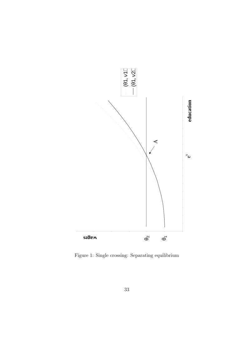
One can define es by picking as signal the least-cost level of educationthat will differentiate more and less productive workers, as Figure 1 shows.

<please insert Figure 1. Single crossing: Separating equilibrium>The least cost separating signal is determined by the less productive

worker with a high taste for study, at point A in Figure 1. At this point,worker type (θ1, ν2) is indifferent between getting a high wage w = θ2 with

6The Appendix discusses condition (ii) for the NxN case of a finite number of types.With a continuum of types θ and ν, condition (ii) is impossible to fulfill unless the rangeof variation of ν is null.

8

education e = es, and a low wage w = θ1 with education e = 0. It is con-sistent with a Nash equilibrium to assume a worker will not signal when itis just indifferent (to break indifference, it would suffice to consider a signales + ε, with ε > 0 that is arbitrarily small). More productive workers strictlyprefer to signal and get a high wage, rather than not signal and get a lowwage.

Given our specification for out-of-equilibrium beliefs, neither type of workerhas an incentive to choose any other level of education because it wouldstrictly reduce its utility. Hence, behavior will conform to (9), so this isindeed a separating equilibrium. The inefficient separating equilibria withlevels of education es > e can be discarded by application of the Cho-Krepsintuitive criterion.7

A pooling equilibrium w = E(θ), where all workers are paid the averageproductivity of the pool of workers, can be discarded as shown in Figure 2.This pooling equilibrium implies that, whatever the level of education, firmswill infer that expected productivity is E(θ). However, the farthest thata low productivity worker is willing to deviate is point B, with educationed. High productivity workers have lower signaling costs, so they can bebetter off to the right of that point. Since those deviations are dominated inequilibrium for less productive types but not for more productive types, bythe intuitive criterion firms can infer that a worker has high productivity iflevels of education larger than (or equal to) ed are observed. That restrictionon out-of-equilibrium beliefs destroys any pooling equilibrium.

<Please insert Figure 2. Single crossing: No pooling equilibrium>Likewise, one can discard partially pooling equilibria where some of the

types are bunched together, namely: the three types with highest ξ choosethe same high signal, or the two intermediate types of ξ choose the sameintermediate signal, or the three types with the lowest ξ pick the same lowsignal. The reason is that the indifference curves of more productive workersare flatter than the indifference curves of less productive types, so moreproductive workers will always be willing to deviate farther to the right thanless productive workers to signal their type.

7There are a multiplicity of separating equilibria with more education than es. How-ever, these Perfect Bayesian Equilibria do not satisfy the intuitive criterion: the out-ofequilibrium beliefs would imply that low productivity workers can signal with positiveprobability in the interval to the right of es to get a high wage, when in fact that is dom-inated in equilibrium by not signaling and getting a low wage. Only high productivityworkers will be willing to pick signals in that interval to get a high wage.

9

These results can be summarized as follows.

Proposition 2 If single-crossing under two-dimensional heterogeneity holds,there is a unique perfect Bayesian equilibrium that satisfies the intuitive cri-terion. This is a separating equilibrium where less productive workers pickzero education and more productive workers pick a positive level of educationthat is just enough to signal their type.

Hence, with a high signal-to-noise ratio the signaling results of the basicSpence model are robust to two-dimensional asymmetric information. In thisinterval, only the Riley outcome –the undominated separating equilibrium–survives refinements of the perfect Bayesian equilibrium that apply the intu-itive criterion.

2.4 No single-crossing

In the interval h ∈ (h, H], condition (7) is no longer satisfied and the rankingof the two intermediate types is inverted:

(11) θ1ν1 < θ2ν1 < θ1ν2 < θ2ν2.

More productive workers no longer have lower costs of signaling. Once theextended single-crossing condition does not hold, no separating equilibriumexists. Why not is easy to see from Figure 3: a worker of type (θ2, ν1) is notwilling to go farther than point C in Figure 3, while a worker of type (θ1, ν2)is. That is, when the ranking is inverted, a less productive worker with hightaste for study is willing to invest in more education than a productive workerwith low taste for study.

<please insert Figure 3. No single crossing: No separating equilibrium>A pooling equilibrium can be discarded as before by application of the

intuitive criterion: a productive worker of type (θ2, ν2) will always be willingto deviate. A partially pooling equilibrium where type (θ1, ν1) worker pickszero education and the other three types with highest ξ pick a commonpositive level of education can be ruled out by a similar argument. However,two other logical possibilities for partially pooling equilibria cannot be ruledout. First, intermediate types pick an intermediate level of education, whileother types pick either zero or high education. Second, all types except(θ2, ν2) pick zero education.

10

First, consider a partially pooling equilibrium with three signals. Type(θ1, ν1) picks zero education, e = 0. Intermediate worker types (θ1, ν2) and(θ2, ν1) send the same intermediate signal ei. Finally, type (θ2, ν2) picks thehighest level of education es. Beliefs µ(.) are given by:

(12) { e = 0 ⇒ µ(θ = θ1|e = 0) = 1e = ei ⇒ µ(θ = θ1|e = ei) = p12

p12+p21

e = es ⇒ µ(θ = θ2|e = es) = 1

.

For out-of-equilibrium levels of education, we assume expected produc-tivity equals that of the lowest level of education within each interval. Out-of-equilibrium beliefs are:

(13) { 0 < e < ei ⇒ µ(θ = θ1|e) = 1ei < e < es ⇒ µ(θ = θ1|e) = p12

p12+p21

e > es ⇒ µ(θ = θ2|e) = 1

.

Expected productivity if an individual has intermediate education is E[θ|e =ei] = p12θ1+p21θ2

p12+p21. The equilibrium with the least-cost signals ei and es is rep-

resented graphically in Figure 4, where θi ≡ p12θ1+p21θ2

p12+p21.

<please insert Figure 4. No single crossing: Partially pooling equilibrium>In the spirit of the Riley outcome, let the least-cost intermediate signal

be determined at point D, with education e = ei and average wage wi = θi,on the indifference curve of type (θ1, ν1) that goes through point e = 0 andw = θ1. And let the least-cost high signal be determined at point E, wheretype (θ1, ν2) is just indifferent between point D and education e = es withwage w = θ2. It is easy to show that no type will want to deviate. Giventhese levels of expected productivity, firms will be willing to actually paythese wages. However, this partially pooling equilibrium is not unique.8

8Cho and Kreps (1987) remark for the Spence signaling model with three types ofproductivity that the intuitive criterion is not always strong enough to ensure the Rileyoutcome. Similarly, here an intermediate signal in the range between point D in Figure4 and the point where the indifference curve of type (θ2, ν1) through coordinates (0, θ1)cuts the intermediate wage line (call it D′) may also satisfy (12), with the high signalnow determined where the indifference curve of type (θ1, ν2) through point D′ cuts thehigh wage line (call this point E′). The only equilibria that can be ruled out over theinterval [D, D′] are those where the highest possible wage for type (θ1, ν1), w = θ2, is at

11

Second, for some parameter values there might be another partially pool-ing equilibrium where the three types with lowest ξ pick zero education, andtype (θ2, ν2) picks a positive level of education es.9 Let equilibrium beliefsbe:

(14) { e = 0 ⇒ µ(θ = θ1|e = 0) = p11+p12

p11+p12+p21

e = es ⇒ µ(θ = θ2|e = es).

For out-of-equilibrium levels of education, we assume expected produc-tivity equals that at the lowest level of education within each interval. Out-of-equilibrium beliefs are:

(15) { 0 < e < es ⇒ µ(θ = θ1|e) = p11+p12

p11+p12+p21

e > es ⇒ µ(θ = θ2|e) = 1.

Expected productivity if an individual has no education is E[θ|e = 0] =(p11+p12)θ1+p21θ2

p11+p12+p21. The partially pooling equilibrium with the least-cost signal

es can be constructed by an argument similar to Figure 4. This is a perfectBayesian equilibrium because no type of worker is willing to deviate. Addi-tionally, there are other equilibria that are less efficient, so it is not uniqueequilibrium.10

The intuitive criterion is not always capable of ruling out partially poolingequilibrium (14). Let θlow ≡ (p11+p12)θ1+p21θ2

p11+p12+p21, and θi ≡ p12θ1+p21θ2

p12+p21. It is

possible to rule out this equilibrium if the education-wage pair (ed, θ2) thatleaves type (θ1, ν1) indifferent to education-wage pair (0, θlow) is such thattype (θ2, ν1) prefers (ed,θi) to alternative (0, θlow). Figure 5 illustrates thecase when it is possible to rule out this equilibrium. This will depend on

an education level that leads to a point below the indifference curve that gives this typeits equilibrium payoff. In that case, equilibrium dominance arguments can be used to ruleout this type. However, since indifference curves of type (θ1, ν1) do not become verticalat D, there always remains a non-empty interval to the right of D over which equilibriumdominance arguments have no bite.

9I thank Gustavo Maradona for pointing this out.10Namely, it is possible to have equilibria where the three types with lowest ξ pick some

positive level of education, together with out-of-equilibrium beliefs that assign individu-als with no education low productivity. These socially less efficient equilibria cannot bediscarded by the intuitive criterion.

12

specific parameter values, requiring sufficiently large θ2 or sufficiently smallp12

p12+p21.

<please insert Figure 5. No single crossing: Alternative partially poolingequilibrium?>

Consequently, we have established the following result:

Proposition 3 If single-crossing under two-dimensional heterogeneity doesnot hold, multiple perfect Bayesian equilibria satisfy the intuitive criterion.There is a partially pooling equilibrium where types with low θ and ν pick zeroeducation, intermediate types pick intermediate education, and types with highθ and ν pick high education; besides an undominated equilibrium, partiallypooling equilibria with excess education are possible. For some parametervalues there are partially pooling equilibria where types with high θ and νpick high education, while the rest pick low education.

Proposition 2 implies that extreme signals are still effective in conveying aworkers’ type. It is in the middle ground (which may include all but the mostable and motivated employees) that there is noise and imperfect revelationof type. From the viewpoint of firms in our model, the parameter ν basicallyintroduces noise into the signal. The setup without single-crossing can beinterpreted as a case of a low signal-to-noise ratio.

As to the relevance of a partially pooling equilibrium, the Appendix an-alyzes the extended single-crossing condition in the NxN case: for a givenrange of variation of productivity, as the number N − 2 of intermediate pro-ductivity types grows, it becomes impossible to satisfy single-crossing unlessthe range of variation in the second dimension shrinks faster (and disappearsin the limit). How serious the issue of noise is will depend on the relativerange of variation of each dimension: perhaps only close productivity typesare bunched together, or instead very distant productivity types are.

3 Employment relationships as signs

If education is indeed a noisy signal, signaling via education will lead to apartially pooling equilibrium. This information could be specially relevantto determine entry requirements (again, we are abstracting from the role ofeducation in the buildup of human capital, that enhances productivity initself). Afterwards, one would expect firms to use other types of information

13

to sort productive and unproductive workers. In this regard, we explore therole of employment relationships.

The process of revelation of productivity at work takes time, so to in-corporate this feature requires a minimum of dynamics. To incorporate theinformation generated in an employment relationship, we assume there aretwo periods. The first period represents the early work career, while thesecond period represents the later work career. A workers’ utility dependson wages wt in periods t = 1, 2, as well as on the cost of education c. Theparameter δ ≤ 1 represents the discount factor, while l ≥ 1 represents thelength of the later work career in relation to the early work career (in caseboth have same length, l = 1).

(16) U(w1, w2, e, θ, ν) = w1 + δlw2 − c(e, θ, ν).

In the first period, the worker has private information on its productivityand signals with a given education level. Firms then make job offers condi-tional on educational levels. After the first period has elapsed, the employerobserves the worker’s true productivity. Employment relationships may turnthis private information into public information in the second period.

We analyze how the revelation of information is related to wage-setting.We consider two polar cases, sticky and flexible wages. As to their relevance,Gottschalk (2005) explains a lot of the evidence on nominal wage flexibility interms of measurement error. Bewley (2002) reports that wage cuts, defined asthe reduction in the pay of an employee continuing to work under unchangedconditions, is low according to surveys of employers from several countries,and is negligible in the few existing studies of company records.

The arrangements on sticky wages may depend on fairness considerations,as in the Akerlof and Yellen (1988) fair wage/effort hypothesis. Indeed, Bew-ley (2002) reports that surveys of business managers responsible for compen-sation policy show that employers avoid cutting pay because doing so wouldhurt morale and goodwill, and hence productivity. It may well be that dif-ferent corporations follow different norms of fairness, so not all need applythe same policy. Nevertheless, if most notions of fairness consider wage cutsunfair and lead to a reduction of work effort, this could lead to a prevalenceof sticky wages in most firms.

Even if nominal wages are mostly sticky, an inflationary environmenthelps to flexibilize real wages, which are the relevant variable for the dis-

14

missal decision. In this regard, Gibbons and Waldman (1999) mention sev-eral studies that show real wage decreases are not rare, though demotionsare.

Rather than analyze wage decisions, we will focus on the choice of theemployer among wage policies (the employer also follows an employmentpolicy that determines employment relationships). That is, an employer willset a rule, conditional on a worker’s productivity, that will determine whetherthe wage is changed or not in the second period. Though a given wage policycan be seen as an ex-ante commitment that defines what an employer willdo when productivity is revealed, the firm is free to pick its best wage policy(not all rules may be equally credible). The informational requirements forother firms of observing the employer’s wage policy are smaller than observingwage decisions, because they do not need to know the specific wages that eachemployee is receiving. Furthermore, if other firms observed each individualwage offers, this would provide additional information on employees that goesbeyond information contained in employment relationship.

3.1 Sticky wages

Suppose that wages are sticky, so firms cannot reduce the wages of theiremployees. In the context of this restriction, a firm that maximizes profitsmight want to dismiss (lay off or fire) in the second period workers whosefirst-period contract stipulates a wage larger than their productivity. To notenter into the issue of the duration of unemployment spells, we will simplyassume that either there is a sign of continued employment relationship ornot.

In the second period, the timing is that the informed firm (the employer)decides its employment policy, setting a cutoff productivity level below whichworkers are dismissed. For those workers who qualify for a renewal of theircontract, the employer determines a wage policy conditional on worker type(the employer can offer a wage hike). The outside firm (that represents thecompetive market) observes the employment policy and the wage policy, andtakes this information into account when defining its wage policy. Finally,the employer observes true productivity, which will determine whether theworker is dismissed or not, and workers who are not dismissed have to decidebetween staying on the job or switching firms.

We can solve the game by backwards induction. Workers will accept thehighest job offer they get (one can assume that if workers are indifferent, they

15

do not switch jobs). It is immediate to see what happens if the first-periodequilibrium is separating: first-period wages equal productivity of workers,so outside firms will be willing to pay that same wage. Employers will matchthat, and offer to renew the contracts of all workers.

On the other hand, if the first-period equilibrium is partially pooling asin (12), there is a signal of intermediate education that corresponds to a mixof productive and unproductive workers.11 Figure 6 depicts this case. Wecondider three employment policies: dismiss all these workers (d, d), dismissless productive workers θ1 whose productivity is below their first-period wage(d, n), or not dismiss any workers (n, n).

<please insert Figure 6. Employment and wage policies of informed anduninformed firms>

The policy of dismissing less productive workers (d, n) will indicate thatdismissed workers have low productivity, and the rest have high productivitybecause there are only two types of productivity (we show below that em-ployer will not prefer alternative employment policies). The outside firm cancondition its wage offer on whether the worker is dismissed or not: it willbe willing to pay dismissed workers a low wage θ1, and continuing workersa high wage θ2. Consequently, the employer has to offer its more produc-tive workers a second-period wage equal to their productivity. This meansthat the employer will make zero profits on its continuing employees. Thus,regardless of whether the first period equilibrium is separating or partiallypooling, in the second period there is an equilibrium where high productivityworkers get a high wage and low productivity workers a low wage equal totheir productivity.

Proposition 4 With 2 productivity types, if wages are sticky there is anequilibrium where employment relationships reveal an employer’s private in-formation on productivity, so wages equal productivity in the second period.

We can now analyze the first-period equilibrium. The solution is straight-forward if the second-period equilibrium reveals the employer’s private infor-mation. The key observation is that, if in the second period wages dependon underlying ability that is fully revealed to the market, wages are indepen-dent of education. That is, education only affects wages in the first period.The first period equilibrium can thus be analyzed as in Section 2, where the

11For some parameter values, partially pooling equilibrium (14) with two signals is alsopossible. The analysis would be similar to that in text.

16

interpretation is now that the costs of education have to be compared to thebenefits in the early job career (period one).

As to alternative employment polices, foreseeing that dismissals revealproductivity, employers could decide not to dismiss anybody. Indeed, as analternative, the employer can keep all workers, paying them θi (if it payedmore, in expected value it would lose money). The outside firm will bewilling to match that, since it will make zero profits. The employer can alsodismiss all workers, in which case the outside firm will be willing to pay themtheir expected productivity θi. Since any of the three employment policies inFigure 6 leads to zero expected profits, the employer is in principle indifferentamong them. However, the equilibria where employment relationships do notreveal an employers private information on productivity are not credible ex-post.12 Furthermore, beyond 2 productivity types, the employment policyof discriminating between low and high productivity workers will providepositive rents, so it will be strictly preferred by the employer to the otherpolicies where expected profits are always zero.13

3.2 Flexible wages

What happens if firms can reduce the wages of employees who are found tohave low productivity? In that case, the outside firm will not be able todistinguish high and low productivity workers by their employment relation-ships, because there is no need of dismissing unproductive workers.

The second period timing is that the employer first decides its wage pol-icy. The employer can condition its wage offer on the productivity type eachemployee has. The second-period offer may be either larger or smaller thanthe first period wage since there are no restrictions on wage cuts. The unin-

12Ex-post, the employer may want to switch policies: if revealed productivity of itsemployees with intermediate education were below the first period wage, it would notwant to keep them all; if revealed productivity were above the first period wage, it wouldnot want to dismiss them all.

13If we analyzed employment and wage policies instead, the result would be prettysimilar. There is an equilibrium where the employer dismisses less productive employees,and keeps more productive employees with a wage of θ2, when outside firms offer to paycontinuing workers θ2 whatever the wage offer of the employer. Dismissing all workers is anequilibrium if outside firms offer θ2 to all continuing workers. Not dismissing any workers,offering them all θi, is only an equilibrium if all workers switch to outside firms when wageoffers match (an assumption opposite to that made in text). In all three equilibria, theemployer makes zero profits ex-post.

17

formed firm does not observe the exact offer the informed firm makes to eachemployee, but it observes the wage policy, in terms of what wages are offeredto each type of worker. On the basis of the employer’s wage policy, outsidefirms make the employees an unconditional counteroffer, which they cannotcondition on the worker’s type because this is inside information. Finally,each type of worker has to decide between staying on the job or switchingfirms.

We can solve the game by backwards induction. Workers will accept thehighest job offer they get. Again, it is immediate to see what happens if thefirst-period equilibrium is separating. Outside firms will be willing to pay thefirst-period wages, which equal productivity. The employer will match that,offering a renewal of contracts. We assume that workers who are indifferentdo not switch jobs.

On the other hand, if the first-period equilibrium is partially pooling,there is a signal of intermediate education that corresponds to a mix of moreand less productive workers. Less productive workers will face a wage cut,since the employer will not be willing to pay more than θ1. However, theemployer has more options for more productive workers θ2: schematically,it can offer to raise the wage, to reduce it, or to maintain it at level offirst-period wage θi = p12θ1+p21θ2

p12+p21. This is represented in Figure 7.14

<please insert Figure 7. Wage policies of informed and uninformed firms>For simplicity, the representation is restricted to conditional strategies

where the informed firm always offers low productivity workers a low wage.On the other hand, it can offer high productivity workers either the samewage θi as in the first period, a low wage θ1 (the same logic will apply to anyother low wage), or a high wage θ2 (the same logic will apply to any otherhigh wage). As to the unconditional strategies of uninformed firms, they canoffer wages between θ1 and θi (any wage higher than θi would lead them tolose money). For simplicity, we only represent the two endpoints.

In view of these logical possibilities, if the employer offers type θ2 employ-ees a raise above θi, uninformed firms will have an incentive to offer a lowwage equal to θ1, because at any wage equal to or lower than the expectedproductivity of the pool of workers with intermediate education they willonly attract lemons, losing money. If the employer offers type θ2 employees awage reduction below θi, uninformed firms can offer all workers a wage thatis slightly higher (up to θi), attracting the whole pool and still making a

14The analysis for the partially pooling equilibrium with two signals is similar.

18

profit. The last possibility is to offer type θ2 employees the same wage θi asin period one. If we assume for simplicity that a worker does not switch jobswhen indifferent (to not have to add ε to break tie), then uninformed firmshave an incentive to offer a low wage equal to θ1: at a wage equal to averageproductivity θi of pool they would only attract lemons, loosing money.

Given this maximizing behavior of uninformed firms, namely, offering θi

to pool of workers if the employer offers more productive workers less thanθi, and offering θ1 if employer offers them θi or more, the informed firm hasan incentive to pick the conditional strategy of offering type θ1 workers awage equal to their productivity θ1, and type θ2 workers the same wage θi asin the first period. Consequently,

Proposition 5 With 2 productivity types, if wages are flexible employmentrelationships do not reveal an employer’s private information on productivity.If the first period signaling game is separating, wages equal productivity inthe second period. If the first period signaling game is partially pooling, theemployer will have an informational rent on some high productivity workers,while other wages will equal productivity in the second period.

The main insight from flexible wages is that, if employers can use condi-tional wage strategies, information on productivity may remain private evenwhen there are only two types of productivity. The employer will have aninformational monopoly: the informed firms will be under no pressure toraise the wage of productive workers with intermediate education. Hence,the informed firm can engage in cream-skimming, paying more productiveworkers with less education below their full productivity. Given this secondperiod outcome, wages for productive workers in the second period will notbe independent of education.15

15Our analysis differs from Gibbons and Katz (1991), because we consider wage poli-cies instead of wage offers, and two productivity types instead of a continuum of types.For wage offers with two productivity types, one can find the following equilibrium: theemployer offers a wage θ1 to θ1 type workers, and plays a mixed strategy of offering θ2

type workers either a wage of θ1 or a wage larger than θ1 (which can be as large as θ2).The uninformed firm offers a wage equal to expected productivity of pool of workers thatreceive a wage offer of θ1, and a wage θ2 to workers that receive any wage offer largerthan θ1. Given these strategies, both the employer and the uninformed firms are makingzero profits, and neither has an incentive to deviate. Hence, with 2 productivity types, ifuninformed firms observe individual wages there will be no rents, instead of positive rentswhen they only observe wage policy. This makes sense because individual wages convey

19

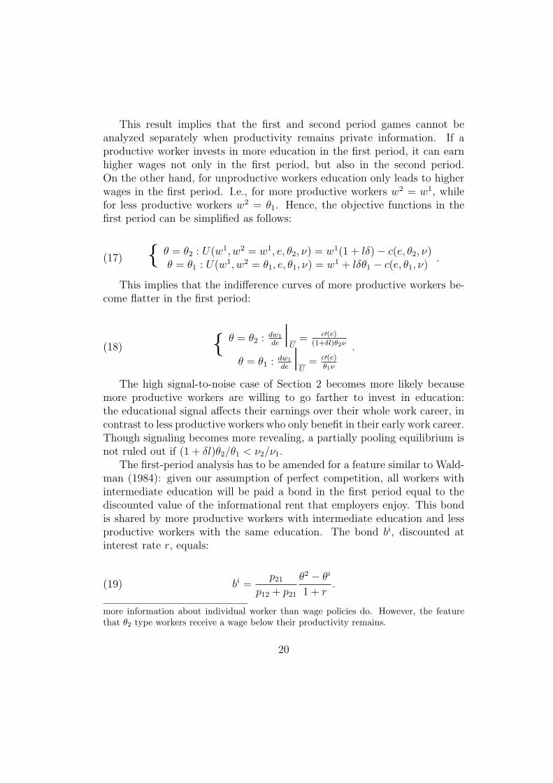
This result implies that the first and second period games cannot beanalyzed separately when productivity remains private information. If aproductive worker invests in more education in the first period, it can earnhigher wages not only in the first period, but also in the second period.On the other hand, for unproductive workers education only leads to higherwages in the first period. I.e., for more productive workers w2 = w1, whilefor less productive workers w2 = θ1. Hence, the objective functions in thefirst period can be simplified as follows:

(17) { θ = θ2 : U(w1, w2 = w1, e, θ2, ν) = w1(1 + lδ)− c(e, θ2, ν)θ = θ1 : U(w1, w2 = θ1, e, θ1, ν) = w1 + lδθ1 − c(e, θ1, ν)

.

This implies that the indifference curves of more productive workers be-come flatter in the first period:

(18) { θ = θ2 : dw1

de|

U= c′(e)

(1+δl)θ2ν

θ = θ1 : dw1

de|

U= c′(e)

θ1ν

.

The high signal-to-noise case of Section 2 becomes more likely becausemore productive workers are willing to go farther to invest in education:the educational signal affects their earnings over their whole work career, incontrast to less productive workers who only benefit in their early work career.Though signaling becomes more revealing, a partially pooling equilibrium isnot ruled out if (1 + δl)θ2/θ1 < ν2/ν1.

The first-period analysis has to be amended for a feature similar to Wald-man (1984): given our assumption of perfect competition, all workers withintermediate education will be paid a bond in the first period equal to thediscounted value of the informational rent that employers enjoy. This bondis shared by more productive workers with intermediate education and lessproductive workers with the same education. The bond bi, discounted atinterest rate r, equals:

(19) bi =p21

p12 + p21

θ2 − θi

1 + r.

more information about individual worker than wage policies do. However, the featurethat θ2 type workers receive a wage below their productivity remains.

20

This bond bi has to be reckoned with in the computation of the firstperiod equilibrium: type (θ2, ν1) has to forego this bond if it switches fromintermediate signal ei to high signal es, while type (θ1, ν2) gets this bond ifit switches from low signal e = 0 to intermediate signal ei. Hence, in someborderline cases there may be a partially pooling equilibrium, instead of aseparating equilibrium, because of this bond.

3.3 Empirical implications

Under sticky wages, Table 2 shows there is a positive correlation betweeneducation and wages: more highly educated workers on average get higherwages in the second period. Hence, even if education is a noisy signal, thestandard implication of Spence (1973) stands over time. Second, there isa positive correlation between employment relationships (workers who havenot been dismissed) and wages. That is, dismissed workers earn less, andthis effect is important for people with more education. This is preciselythe empirical pattern of layoffs and lemons so nicely studied by Gibbons andKatz (1991).

<please insert Table 2. Second period wages with public information>Under flexible wages, Table 3 shows that there is also a positive correlation

between education and wages: more highly educated workers on average gethigher wages in the second period (w1,i stands for the wage that individualswith intermediate education receive in periods 1 and 2). However, workerswith the same productivity and different education may earn different wages,due to the informational rents that employers enjoy.

<please insert Table 3. Second period wages with private information>If the first period were only a short probationary period where the em-

ployer could gather all the relevant information on productivity, educationwould not be very relevant as a job-market signal. For the present frame-work to add empirically relevant insights, the early work career has to berelatively extensive in relation to the later work career. In this regard, apartially pooling equilibrium with three signals in the first period impliesa growth over time of the variance of wages for higher educational levels,because in the second period some workers with intermediate education gethigh wages and others get low wages.16 This can be related to Mincer (1974),

16This would not happen in the partially pooling equilibrium with two signals. However,since for some parameter values this equilibrium does not exist, in the text we concentrate

21

who has a table based on 1960 U.S. Census (reproduced in Weiss 1983) thatshows that while the variance of the log of weekly earnings hardly changesfor people with 5-8 years of schooling, for people with 12 years of schoolingit rises smoothly but steadily, from .205 at ages 24-29 to .317 at ages 55-59.And for people with 16 years of schooling, where signaling can be expectedto be especially important because of the more autonomous nature of jobs,the variance rises a lot: from .235 for 24-29 year-old group and .277 for 35-39year-old group, to .424 for 45-49 year-old group, and .552 for 55-59 year-oldgroup. Albeit indirectly, the fact that the variance in earnings for peoplewith 16 years of schooling at first does not rise much might indicate that theearly work career could represent a period of up to 10 or 15 years.

Ashenfelter and Krueger (1994) find that returns to education for identi-cal twins may be as large as for the population as a whole, which in the line ofhuman capital models can be interpreted as isolating the effect of educationon earnings, controlling for ability. Weiss (1995) also offers a sorting expla-nation: firms will infer a worker’s unobserved ability from the educationalchoice, so education should affect initial wages according to the signalingmodel. Weiss goes on to say that if the signaling model is correct, the returnto schooling across twins should decline over time, and he finds some evidencein that direction. However, the results above show that the implication of thesignaling models critically depend on whether the employer’s private infor-mation becomes public or not: if it becomes public, wage differences shoulddecline over time, but if it doesn’t, wage differences will not decline.17 Theimplication of private information is that wages need not match productivity,because the employer’s private information leads to informational rents. Inthis context, education as a signal will not only affect the wages of more ableworkers in their early job career, but rather over their whole career.

In the 2x2 case, productivity becomes public information with stickywages regardless of education in the first period, while with flexible wagesproductivity remains private information for intermediate types. If stickywages are prevalent, an implication is that there should be less dismissalsunder an inflationary environment than under stable prices, because inflation

on the partially pooling equilibirum with three signals.17In fact, the model with flexible wages implies that difference will increase, because

workers with intermediate education are paid an extra bond in the first period equal toexpected discounted value of the informational rent in the second period. Wages thatdecline over the life-cycle are counter-factual, but we are abstracting from the positiveinfluence of experience and human capital on earnings.

22

is a real-wage reducing device. This may also be a specific example in whichinflation can contribute to make prices (here, wages) less informative.

When there are more than two productivity types, the Appendix showsthat the result on full revelation of employer’s private information throughemployment relationships under sticky wages does not hold. This is notsurprising: in a different setup, Gibbons and Katz (1991) show that with acontinuum of productivity types, dismissals only reveal that workers with acontinuing employment relationship have productivity above a certain cut-off level. What is true is that more information is always revealed understicky wages than under flexible wages. The key intuition is that uninformedfirms are always willing to pay the pool of continuing workers their expectedproductivity, which exceeds first-period wage under sticky wages, but equalsfirst-period wage with flexible wages. The higher wage offers that uninformedfirms are willing to make under sticky wages limit the informational rents ofthe informed firm.

The fact that on-the-job productivity does not fully become public in-formation might help explain the role of an MBA, where people with workexperience enroll. In comparison to other graduate programs, an MBA hasless of a human capital role, and more of a signaling role. Indeed, some par-ticipants in the process describe it as basically going around from one meetingto another with corporate representatives. Such a limited role can make per-fect sense to those students that basically need the MBA as a system-widesignal to reveal their ability, if their work record does not accomplish thatfor them. By (18), even if ability did not reduce the costs of education, highproductivity agents would still have lower signaling costs because educationincreases their life-time earnings. This leads to self-selection: only peoplewho believe they are high-ability have a large incentive to invest in an MBAas a job-market signal.

4 Conclusions

This paper analyzes the implications of two-dimensional asymmetric infor-mation for Spence’s (1973) signaling model. Both ability and an idiosyncraticfactor, called taste for study, can be either high or low. An extended single-crossing condition is satisfied when the ranking of signaling costs is basicallydetermined by ability. When there is single-crossing, the equilibrium is sep-arating. When not, the equilibrium becomes partially pooling.

23

The second dimension basically allows to analyze the influence of noiseon the informative content of the signal. If education is indeed a noisysignal, it will be an imperfect proxy for a worker’s productivity so otherinformation will be used by firms. In this regard, the work record is singledout in this paper. Interaction at the work place generates private informationon productivity for the employer. This is modeled in a dynamic settingwhere the first period, which represents the early job career, is the signalinggame. The second period represents the later job career, where employersuse information from the first period to judge productivity.

One way information on work productivity observed by the employer maybecome public is through the Gibbons and Katz (1991) idea on layoffs reveal-ing lemons. Outside firms observe employment relationships. Continuity ofworking relationships can act as a sign of high productivity to other firms ifhigher productivity workers are more likely to keep their job. We find that ifwages are flexible, employment relationships reveal no private information atall. Employers do not need to dismiss lemons, they can simply reduce theirwages.18 With sticky wages, on the other hand, employment relationshipscan be a sign to the market of which employees have high productivity, anddismissals indicate who are lemons.19

When the analysis is extended to consider more types of ability and tastefor study, it becomes harder to satisfy the extended single-crossing condi-tion that ensures education is a separating signal. Unlike the continuouscase with asymmetric information in one dimension (Spence 2002), one canexpect that with asymmetric information and heterogeneity in two dimen-sions, the equilibrium with a continuum of types will never be separating, butrather partially pooling. However, signaling is quite resilient to the introduc-tion of asymmetric information in two dimensions, in the sense that averageproductivity is still increasing in the degree of education, and extreme typesstill send unequivocal signals. However, intermediate types will be difficultto tell apart.

As to the informative role of employment relationships, when one goes

18We analyze in text the case where outside firms observe the employers’ wage policies.The result is similar when outside firms observe individual wages, but there wage offersconvey in themselves additional information about the individual worker’s productivity.

19The model completely ignores that work productivity is in part a matter of matchingthe right person to the right job (Jovanovic 1979). This increases the amount of asymmetricinformation, since a worker does not know its productivity type before hand. Dismissalswill indicate a mismatch, but not necessarily that dismissed workers are lemons.

24

beyond the 2x2 case revelation of information is always incomplete even ifwages are sticky. Hence, employers will have an informational rent, payingsome more productive workers less than their full productivity (under perfectcompetition, firms will in turn pay out a bond, which more able workerswill have to share with the less able). Given incomplete revelation of privateinformation, education becomes important for high ability workers as a signalnot only in their early job career, but over their whole work cycle.

If education is a life-time signal only for individuals with high ability,studying can make perfect sense to them despite the fact they face a largeropportunity cost of not working. The higher opportunity cost is more thancompensated by the larger earnings over the complete career, making signal-ing costs of high ability individuals smaller than those of low ability individ-uals. In other words, a prestigious degree can help to land a good job, butnot to hold on to it, so this leads to self-selection when signaling.

A natural extension of this model is to combine the signaling role of ed-ucation with the human capital role of education (Becker 1964), to derivemore precise empirical implications about the complete effects of formal edu-cation and on-the-job training and experience. There are other signs at workbesides employment relationships. For example, more able workers may beassigned more complicated jobs, or jobs with higher responsibility. If jobhierarchies are visible to outside firms, this can act as a sign of work produc-tivity. This is precisely what Waldman (1984) proposes: job assignments asa sign of productivity.20

Finally, the present framework considers noise as an example of two-dimensional asymmetric information. This issue is already present in theAkerlof (1970) lemons model: there is a problem with lemons because thereare some dishonest sellers who are willing to misstate the quality of their car.It might be applied to consider the closely related issue of the influence ofcharacter on productivity. Though some traits of character like perseverancemight also be captured by formal education (Weiss 1995), others will not.

20Waldman also makes the point that, with a continuum of types, job assignments willonly reveal part of this private information to the market, i.e., that those assigned to thehigher productivity job are above a certain ability level.

25

5 Appendix

5.1 Single-crossing in the NxN case

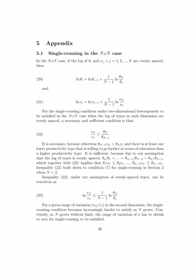
In the NxN case, if the log of θi and νj, i, j = 1, 2, ..., N are evenly spaced,then

(20) ln θi = ln θi−1 +1

N − 1ln

θN

θ1

and

(21) ln νj = ln νj−1 +1

N − 1ln

νN

ν1

For the single-crossing condition under two-dimensional heterogeneity tobe satisfied in the NxN case when the log of types in each dimension areevenly spaced, a necessary and sufficient condition is that:

(22)vN

v1

≤ θN

θN−1

It is necessary, because otherwise θN−1vN > θNv1 and there is at least onelower productivity type that is willing to go farther in terms of education thana higher productivity type. It is sufficient, because due to our assumptionthat the log of types is evenly spaced, θ2/θ1 = ... = θN−1/θN−2 = θN/θN−1,which together with (22) implies that θ1vN ≤ θ2v1, ..., θN−2vN ≤ θN−1v1.Inequality (22) boils down to condition (7) for single-crossing in Section 2when N = 2.

Inequality (22), under our assumption of evenly-spaced types, can berewritten as

(23) lnvN

v1

≤ 1

N − 1ln

θN

θ1

For a given range of variation (vN/v1) in the second dimension, the single-crossing condition becomes increasingly harder to satisfy as N grows. Con-versely, as N grows without limit, the range of variation of ν has to shrinkto zero for single-crossing to be satisfied.

26

5.2 Employment relationships as noisy signs in 3x3 case

Consider a 3x3 example, with three types of productivity θi and three typesof taste for study υj, i, j = 1, 2, 3, where the types are evenly spaced apartso θ2/θ1 = (θ3/θ1)

1/2 and ν2/ν1 = (ν3/ν1)1/2.

Assume that v3/v1 > θ3/θ1, so v2/v1 > θ2/θ1 and v3/v2 > θ3/θ2. Thisis only interesting scenario where there is a qualitative difference with the2x2 case; otherwise, there is no educational signal for which workers of threetypes of productivity can pool together.

Two orderings are possible, either v2/v1 > θ3/θ1, so ranking is basicallydetermined by ν, i.e.,

(24) θ1ν1 < θ2ν1 < θ3ν1 < θ1ν2 < θ2ν2 < θ3ν2 < θ1ν3 < θ2ν3 < θ3ν3,

or v2/v1 ≤ θ3/θ1 so ranking is given by

(25) θ1ν1 < θ2ν1 < θ1ν2 ≤ θ3ν1 < θ2ν2 < θ1ν3 ≤ θ3ν2 < θ2ν3 < θ3ν3.

We will analyze the second case, but the first case would be similar forour purposes.

The distribution of types detailed in Table 4 will determine how the dif-ferent types group.

<please insert Table 4. Probability distribution in 3x3 case>Without entering into a full characterization of possible equilibria, let ei

denote education level, with five levels, e0 < e1 < e2 < e3 < e4, e0 = 0, whereeach ei is associated to the following expected productivity:

(26) {e = 0 ⇒ E[θ|e = 0] = θ1

e = e1 ⇒ E[θ|e = e1] = p12θ1+p21θ2

p12+p21

e = e2 ⇒ E[θ|e = e2] = p13θ1+p22θ2+p31θ3

p13+p22+p31

e = e3 ⇒ E[θ|e = e3] = p23θ2+p32θ3

p23+p32

e = e4 ⇒ E[θ|e = e3] = θ3

In a manner similar to Figure 4, one can define each successive ei, i =1, 2, 3, as the least-cost signal such that no type has an incentive to deviate.For this to be a perfect Bayesian equilibrium, expected productivity has to

27

be strictly increasing in the signal. If not, either types grouped at e3 wouldprefer to deviate to e2, or types grouped at e2 would prefer to deviate toe1, or both. This would reduce the number of educational signals from fiveto either four or three, producing even more bunching of types. Other thanthis, the analysis would be similar to equilibrium (26).

In equilibrium (26), only the extreme type (θ3, ν3) goes far enough tosingle itself out with an educational signal. For all the types in betweentypes (θ3, ν3) and (θ1, ν1), there will be some bunching (in the extreme, theywill all pick the same signal), so it will not be possible to tell them perfectlyapart.

Take the case where wages are sticky (if wages were flexible, we alreadyknow that employment relationships reveal no information at all). If thepartially pooling equilibrium in the first period were given by (26), Willwages in the second period still be independent of education (as happenedin Section 3)?

In the second period the employer will have an incentive to dismiss work-ers whose productivity is lower than their wage. This will perfectly reveal theworker’s exact productivity for intermediate educational level e2 (e4): thosedismissed have productivity θ1 (θ2), so those retained have productivity θ2

(θ3).However, this sign does not work perfectly for educational level e3. The

expected productivity of workers with education e3 is either above or belowθ2. If (i) it is equal to, or less than, θ2, the employer will dismiss typeθ1 employees. This will reveal the type of dismissed workers, but not ofcontinuing workers, of whom the market only knows that their expectedproductivity is

(27) E[θ|e = e3, not dismissed] =p22θ2 + p31θ3

p22 + p31

.

If the employer offers type θ3 less than (27), the uninformed firms willfind it profitable to attract the whole pool of continuing workers, offering an εmore (the analysis is similar to Figure 6). Hence, the employer will be willingto pay type θ3 a wage equal to expected productivity of pool, namely (27),and type θ2 a wage of θ2. Given these conditional wage offers of the informedfirm, the optimal response of uninformed firms is to offer θ2 to the pool; ifthey offer more, they will lose money. This result implies that employmentrelationships will never allow the market to differentiate between type (θ3, ν1)

28

and type (θ2, ν2), so earnings of type (θ3, ν1) will depend on education in thelong run.

What would happen if the expected productivity of types that pick e3

were (ii) larger than θ2? In that case, type (θ2, ν2) would be dismissed to-gether with type (θ1, ν3), so outside firms would only be willing to pay poolof dismissed workers their expected productivity. For total revelation ofproductivity of the lower productivity types, one would need to add morerounds.

In either case, employment relationships only lead to partial revelationof the employer’s private information. However, while (ii) has transitoryconsequences, (i) has permanent consequences because adding more periodswould not change the state of affairs. Hence, even if wages are sticky, withthree types of productivity dismissals no longer produce full revelation oftypes. This relates to the Gibbons and Katz (1991) results for a continuumof productivity levels.

To determine whether the first period equilibrium in a dynamic setupwill indeed be as specified in (26), one has to incorporate the long-termvalue of education for more able workers in the first period signaling game.If the problem of noise is strong enough, it will still be possible to find anequilibrium for which there is bunching of workers with different productivitylevels in the first period.

References

[1] Akerlof, George. “The market for ‘Lemons’: Quality uncertainty andthe market mechanism.” Quarterly Journal of Economics, August 1970,84(3): 488-500.

[2] Akerlof, George, and Yellen, Janet. “Fairness and unemployment.”American Economic Review, May 1988, 78(2): 44-49

[3] Ashenfelter, Orley, and Alan Krueger. “Estimates of the economic returnto schooling from a new sample of twins.” American Economic Review,December 1994, 84(5): 1157-1173.

[4] Becker, Gary S. Human Capital: A Theoretical and Empirical Analysis,with Special Reference to Education. New York, NY: Columbia Univer-sity Press (for NBER), 1964.

29

[5] Behrenz, Lars. “Who gets the job and why. An explorative study of em-ployers’ recruitment behavior.” Journal of Applied Economics, Novem-ber 2001, 4(2): 255-278.

[6] Bewley, Truman F. “Fairness, reciprocity, and wage rigidity.” October2002, Cowles Foundation Discussion Papers 1383, Yale University.

[7] Cho, In Koo, and David M. Kreps. “Signaling games and stable equi-libria.” Quarterly Journal of Economics, May 1987, 102(2): 179-221.

[8] Edlin, Aaron S. and Chris Shannon. “Strict single crossing and the strictSpence-Mirrlees condition: A comment on monotone comparative stat-ics.” Econometrica, November 1998, 66(6): 1417-25.

[9] Fudenberg, Drew, and Tirole, Jean. Game Theory, Cambridge, MA:MIT Press, 1991.

[10] Gibbons, Robert and Lawrence F. Katz. “Layoffs and lemons.” Journalof Labor Economics, October 1991, 9(4): 351-81.

[11] Gibbons, Robert and Michael Waldman. “A theory of wage and promo-tion dynamics inside firms.” Quarterly Journal of Economics, November1999, 114(4): 1321-58.

[12] Gottschalk, Peter. “Downward nominal wage flexibility: Real or mea-surement error?” Review of Economics and Statistics, August 2005,87(3): 556-68.

[13] Jovanovic, Boyan. “Job matching and the theory of turnover.” Journalof Political Economy, October 1979, 87(5): 972-990.

[14] Mincer,Jacob A., Schooling, Experience, and Earnings, New York, NY:Columbia University Press, 1974.

[15] Riley, John G. “Informational equilibrium.” Econometrica, March 1979,47(2): 331-59.

[16] Riley, John G. “Silver signals: 25 years of signaling and screening.”Journal of Economic Literature, June 2001, 39(2): 432-78.

[17] Spence, Michael. “Job market signaling.” Quarterly Journal of Eco-nomics, August 1973, 87(3): 355-379.

30

[18] Spence, Michael. “Signaling in retrospect and the informational struc-ture of markets.” American Economic Review, June 2002, 92(3): 434-59.

[19] Waldman, Michael. “Job assignments, signalling and efficiency.” RandJournal of Economics, Summer 1984, 15(2): 255-67.

[20] Weiss, Andrew. “A sorting-cum-learning model of education.” Journalof Political Economy, June 1983, 91(3):420-442.

[21] Weiss, Andrew. “Human capital vs. signalling explanations of wages.”Journal of Economic Perspectives, Autumn 1995, 9(4): 133-154.

31

Table 1.Probability distribution in 2x2 caseTaste νν1 ν2

Ability θ θ1 p11 p12

θ2 p21 p22

Table 2. Second period wages with public informationWages w2

Education- none θ1

- positive {p12θ1 + (p21 + p22)θ2}/(p12 + p21 + p22)Employment relationship- dismissed θ1

- renewed {p11θ1 + (p21 + p22)θ2}/(p11 + p21 + p22)

Table 3. Second period wages with private informationWages w2

Education- none θ1

- positive (p12θ1 + p21w1,i + p22θ2)/(p12 + p21 + p22)

Ability- low θ1

- high (p21w1,i + p22θ2)/(p21 + p22)

Table 4. Probability distribution in 3x3 caseTaste νν1 ν2 ν3

θ1 p11 p12 p13

Ability θ θ2 p21 p22 p23

θ3 p31 p32 p33

32

0123456

00.

125

0.25

0.37

50.

50.

625

0.75

0.87

51

1.12

51.

251.

375

1.5

1.62

51.

751.

875

2

educ

atio

n

wages

(θ1,

ν1)

(θ1,

ν2)

A

es

θ 2 θ 1

Figure 1: Single crossing: Separating equilibrium

33

0

0.51

1.52

2.53

3.54

4.55

00.

125

0.25

0.37

50.

50.

625

0.75

0.87

51

1.12

51.

251.

375

1.5

1.62

51.

751.

875

2

educ

atio

n

wages

(θ1,

ν2)

(θ2,

ν1)

B

ed

θ 2 E( θ

)

Figure 2: Single crossing: No pooling equilibrium

34

0

0.51

1.52

2.53

3.5

00.

125

0.25

0.37

50.

50.

625

0.75

0.87

51

1.12

51.

251.

375

1.5

1.62

51.

751.

875

2

educ

atio

n

wages

(θ1,

ν2)

(θ2,

ν1)

C

θ 2 θ 1

ed

Figure 3: No single crossing: No separating equilibrium

35

0123456

00.

125

0.25

0.37

50.

50.

625

0.75

0.87

51

1.12

51.

251.

375

1.5

1.62

51.

751.

875

2

educ

atio

n

wages

(θ1,

ν1)

(θ1,

ν2)

Dθ 2 θ 1

ei

E

es

θi

Figure 4: No single crossing: Partially pooling equilibrium

36

0123456

00.

125

0.25

0.37

50.

50.

625

0.75

0.87

51

1.12

51.

251.

375

1.5

1.62

51.

751.

875

2ed

ucat

ion

wages

(θ1,

ν1)

(θ2,

ν1)

F

θ 2 θlow

ed

G

θi

Figure 5: No single crossing: Alternative partially pooling equilibrium?

37

Info

rmed

firm

Out

side

firm

Out

side

firm

Out

side

firm

(d,d

)(d

,n)

(θ1,

θ 2)

θ 1

θ 1θ 2

θi

θi(θ

1,θ 1

)(θ

1,θi )

(n,n

)

θ 2

Info

rmed

firm

Info

rmed

firm

Out

side

firm

θiθ 2

(θ1,

θ 1)

(θ1,

θi )(θ

1,θ 2

)

(θi ,θ

i )(θ

i ,θ2)

Out

side

firm

θ 1θi

θ 2

Figure 6: Employment and wage policies with sticky wages

38

Info

rmed

firm

Uni

nfor

med

firm

Uni

nfor

med

firm

Uni

nfor

med

firm

(θ1,

θ 1)

(θ1,

θi )(θ

1,θ 2

)

θ 1θ 1

θ 1θi

θiθi

Figure 7: Wage policies with flexible wages

39